Numerical Methods for Partial Differential Equationszcai/pdf-paper/16CaCh.pdf · Numerical Methods for Partial Differential Equations Copy of e-mail Notification Numerical Methods

Numerical Methods for Partial Differential Equations Copy of e-mail Notification

Numerical Methods for Partial Differential Equations Published by John Wiley & Sons, Inc. Dear Author, Your article page proof for Numerical Methods for Partial Differential Equations is ready for your final contentcorrection within our rapid production workflow. The PDF file found at the URL given below is generated to provideyou with a proof of the content of your manuscript. Once you have submitted your corrections, the production officewill proceed with the publication of your article. John Wiley & Sons has made this article available to you online for faster, more efficient editing. Please follow theinstructions below and you will be able to access a PDF version of your article as well as relevant accompanyingpaperwork. First, make sure you have a copy of Adobe Acrobat Reader software to read these files. This is free software andis available for user downloading at http://www.adobe.com/products/acrobat/readstep.html. Open your web browser, and enter the following web address:http://115.111.50.156/jw/retrieval.aspx?pwd=fdc916b7aa88 You will be prompted to log in, and asked for a password. Your login name will be your email address, and yourpassword will be fdc916b7aa88 Example: Login: your e-mail addressPassword: fdc916b7aa88 The site contains one file, containing: - Author Instructions Checklist- Annotated PDF Instructions- Reprint Order Information- Color Reproduction Form- A copy of your page proofs for your article In order to speed the proofing process, we strongly encourage authors to correct proofs by annotating PDF files.Any corrections should be returned to [email protected] 1 to 2 business days after receipt of this email. Please see the Instructions on the Annotation of PDF files included with your page proofs. Please take care toanswer all queries on the last page of the PDF proof; proofread any tables and equations carefully; and check that

Numerical Methods for Partial Differential Equations Copy of e-mail Notification

any Greek characters (especially "mu") have converted correctly. Please check your figure legends carefully. - answer all queries on the last page of the PDF proof- proofread any tables and equations carefully- check your figure(s) and legends for accuracy Within 1 to 2 business days, please return page proofs with corrections and any relevant forms to: Production Editor, NUME-mail: [email protected] Technical problems? If you experience technical problems downloading your file or any other problem with thewebsite listed above, please contact Balaji/Sam (e-mail: [email protected], phone: +91 (44) 4205-8810(ext.308)). Be sure to include your article number. Questions regarding your article? Please don't hesitate to contact me with any questions about the article itself, orif you have trouble interpreting any of the questions listed at the end of your file. REMEMBER TO INCLUDE YOURARTICLE NO. ( 22055 ) WITH ALL CORRESPONDENCE. This will help us address your query most efficiently. As this e-proofing system was designed to make the publishing process easier for everyone, we welcome any andall feedback. Thanks for participating in our e-proofing system! This e-proof is to be used only for the purpose of returning corrections to the publisher. Sincerely, Production Editor, NUME-mail: [email protected]

1 1 1 RI V E R S T R E E T, HO B O K E N , N J 0 7 0 3 0

***IMMEDIATE RESPONSE REQUIRED***Your article will be published online via Wiley's EarlyView® service (wileyonlinelibrary.com) shortly after receipt of

corrections. EarlyView® is Wiley's online publication of individual articles in full text HTML and/or pdf format before releaseof the compiled print issue of the journal. Articles posted online in EarlyView® are peer-reviewed, copyedited, author corrected,and fully citable via the article DOI (for further information, visit www.doi.org). EarlyView® means you benefit from the best

of two worlds--fast online availability as well as traditional, issue-based archiving.

Please follow these instructions to avoid delay of publication.

READ PROOFS CAREFULLY• This will be your only chance to review these proofs. Please note that once your corrected article is posted

online, it is considered legally published, and cannot be removed from the Web site for furthercorrections.

• Please note that the volume and page numbers shown on the proofs are for position only.

ANSWER ALL QUERIES ON PROOFS (If there are queries they will be found on the last page of the PDF file.)

CHECK FIGURES AND TABLES CAREFULLY• Check size, numbering, and orientation of figures.• All images in the PDF are downsampled (reduced to lower resolution and file size) to facilitate Internet delivery.

These images will appear at higher resolution and sharpness in the final, published article. • Review figure legends to ensure that they are complete.• Check all tables. Review layout, title, and footnotes.

RETURN PROOFSOther forms, as needed

QUESTIONS Production Editor, NUME-mail: [email protected] to journal acronym and article production number(i.e., NMPDE-0000-0000 for Numerical Methods for Partial Differential Equations ms 00-0000)

• In order to speed the proofing process, we strongly encourage authors to correct proofs by annotating PDF files.Please see the instructions on the Annotation of PDF files. If unable to annotate the PDF file, please print outand mark changes directly on the page proofs.

Return corrections immediately via email to [email protected]

USING e-ANNOTATION TOOLS FOR ELECTRONIC PROOF CORRECTIONTION

Once you have Acrobat Reader open on your computer, click on the Comment tab at the right of the toolbar:

This will open up a panel down the right side of the document. The majority of tools you will use for annotating your proof will be in the Annotations section,pictured opposite. We’ve picked out some of these tools below:

1. Replace (Ins) Tool – for replacing text.

Strikes a line through text and opens up a text box where replacement text can be entered.

How to use it

x Highlight a word or sentence.

x Click on the Replace (Ins) icon in the Annotationssection.

x Type the replacement text into the blue box thatappears.

2. Strikethrough (Del) Tool – for deleting text.

Strikes a red line through text that is to bedeleted.

How to use it

x Highlight a word or sentence.

x Click on the Strikethrough (Del) icon in theAnnotations section.

3. Add note to text Tool – for highlighting a sectionto be changed to bold or italic.

Highlights text in yellow and opens up a textbox where comments can be entered.

How to use it

x Highlight the relevant section of text.

x Click on the Add note to text icon in theAnnotations section.

x Type instruction on what should be changedregarding the text into the yellow box thatappears.

4. Add sticky note Tool – for making notes atspecific points in the text.

Marks a point in the proof where a commentneeds to be highlighted.

How to use it

x Click on the Add sticky note icon in theAnnotations section.

x Click at the point in the proof where the commentshould be inserted.

x Type the comment into the yellow box thatappears.

USING e-ANNOTATION TOOLS FOR ELECTRONIC PROOF CORRECTIONTION

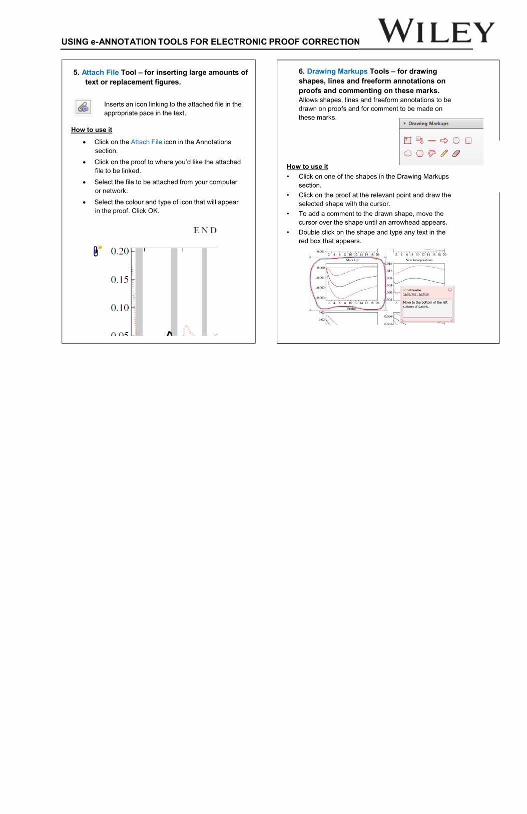
5. Attach File Tool – for inserting large amounts of text or replacement figures.

Inserts an icon linking to the attached file in the appropriate pace in the text.

How to use it

x Click on the Attach File icon in the Annotationssection.

x Click on the proof to where you’d like the attachedfile to be linked.

x Select the file to be attached from your computer or network.

x Select the colour and type of icon that will appear in the proof. Click OK.

6. Drawing Markups Tools – for drawing shapes, lines and freeform annotations onproofs and commenting on these marks.Allows shapes, lines and freeform annotations to be drawn on proofs and for comment to be made on these marks.

How to use it• Click on one of the shapes in the Drawing Markups

section.• Click on the proof at the relevant point and draw the

selected shape with the cursor.• To add a comment to the drawn shape, move the

cursor over the shape until an arrowhead appears.• Double click on the shape and type any text in the

red box that appears.

Should you wish to purchase additional copies of your article, please

click on the link and follow the instructions provided: https://caesar.sheridan.com/reprints/redir.php?pub=10089&acro=NUM

Corresponding authors are invited to inform their co-authors of the

reprint options available.

Please note that regardless of the form in which they are acquired, reprints should not be resold, nor further disseminated in electronic form, nor deployed in part or in whole in any marketing, promotional or educational contexts without authorization from Wiley. Permissions requests should be directed to mail to: [email protected]

For information about ‘Pay-Per-View and Article Select’ click on the following link: wileyonlinelibrary.com/aboutus/ppv-articleselect.html

Additional reprint purchases

Color figures were included with the final manuscript files that we received for your article.Because of the high cost of color printing, we can only print figures in color if authors cover the expense. Please indicate if you would like your figures to be printed in color or black and white. Color imagestwill be reproduced online in Wiley Online Library at no charge, whether or not you opt for color printing. You will be invoiced for color charges once the article has been published in print. Failure to return this form with your article proofs will delay the publication

of your article.

JOURNAL Numerical Methods for Partial Differential Equations MS. NO.

FO .ON COLOR PAGES

TITLE OF MANUSCRIPT

AUTHOR(S)

Color Pages 1 Figure

per Page 2 Figures per Page

3 Figures per Page

4 Figures per Page

5 Figures per Page

6 Figures per Page

1 850 1000 1150 1300 1450 1600

2 1700 1850 2000 2150 2300 2450

3 2550 2700 2850 3000 3150 3300

4 3400 3550 3700 3850 4000 4150

5 4250 4400 4550 4700 4850 5000

6 5100 5250 5400 5550 5700 5850

***Please contact the Production Editor at [email protected] for a quote if you have more than 6 pages

of color***

etihw dna kcalb ni serugif ym tnirp esaelP

$ roloc ni serugif ym tnirp esaelP **International orders must be paid in currency and drawn on a U.S. bank

Please check one: Check enclosed Bill me Credit Card If credit card order, charge to: American Express Visa MasterCard Credit Card No

etaD .pxE erutangiS

BILL TO: Purchase Name Order No.

enohP noitutitsnI sserddA xaF liam-E

0

Least-Squares Method for the Oseen Equation

Zhiqiang Cai, Binghe Chen

J_ID: z8x Customer A_ID: 2015-1785.R2 Cadmus Art: NUM22055 KGL ID:JW-NUMT160006 — 2016/2/23 — page 1 — #1

Least-Squares Method for the Oseen EquationZhiqiang Cai, Binghe ChenDepartment of Mathematics, Purdue University, 150 N. University Street,West Lafayette, Indiana 47907-2067

Received 17 June 2015; accepted 4 February 2016Published online in Wiley Online Library (wileyonlinelibrary.com).DOI 10.1002/num.22055

This article studies the least-squares finite element method for the linearized, stationary Navier–Stokesequation based on the stress-velocity-pressure formulation in d dimensions (d = or 3). The least-squaresfunctional is simply defined as the sum of the squares of the L2 norm of the residuals. It is shown thatthe homogeneous least-squares functional is elliptic and continuous in the H(div; !)d × H 1(!)d × L2(!)

norm. This immediately implies that the a priori error estimate of the conforming least-squares finite elementapproximation is optimal in the energy norm. The L2 norm error estimate for the velocity is also establishedthrough a refined duality argument. Moreover, when the right-hand side f belongs only to L2(!)d , we derivean a priori error bound in a weaker norm, that is, the L2(!)d×d × H 1(!)d × L2(!) norm. © 2016 WileyPeriodicals, Inc. Numer Methods Partial Differential Eq 000: 000–000, 2016

Keywords: a priori error estimate; least-squares method; Navier–Stokes equation; L2 error estimate

I. INTRODUCTION

AQ5

Least-squares finite element methods for the numerical solution of second-order partial dif-ferential equations and systems have been intensively studied by many researchers (see, e.g.,books [1, 2] and references therein). Numerical properties of the least-squares methods depend

AQ3on the form of the first-order system and the choice of the least-squares norms. Basically, thereare three types of the least-squares methods: the inverse approach (see, e.g., [2–4]), the divapproach (see, e.g., [5–7]), and the div-curl approach (see, e.g., [8]). The inverse approach usesan inverse norm that is further replaced by either the weighted mesh-dependent norm (see [9])or the discrete H−1 norm (see [10]) for computational feasibility. The corresponding homoge-neous least-squares functionals for the div and the div-curl approaches are equivalent to theH(div) and the H(div) ∩ H(curl) norms for some variables, respectively. For the Stokes andNavier–Stokes equations, the least-squares methods are based on various first-order systems suchas formulations of the vorticity-velocity-pressure, the stress-velocity, the stress-velocity-pressure,the velocity-gradient-pressure, and so forth.

AQ1

AQ2

Correspondence to: Zhiqiang Cai, Department of Mathematics, Purdue University, 150 N. University Street, WestLafayette, IN 47907-2067 (e-mail: [email protected])Contract grant sponsor: National Science Foundation; contract grant numbers: DMS-1217081 and DMS-1522707

© 2016 Wiley Periodicals, Inc.

ID: annadurai.v Date: 23/2/2016 Time: 10:47 Path: //chenas03/Cenpro/NUM/Vol00000/160006/

NOTE TO AUTHORS: This will be your only chance to review this proof.Once an article appears online, even as an EarlyView article, no additional corrections will be made.

2


2 CAI AND CHEN

In [7], we developed and analyzed the div least-square methods for the stationary Stokesequation. The purpose of this article is to extend our study to the Oseen equations, that is, thelinearized, stationary Navier–Stokes equation. Specifically, we introduce the div least-squaresminimization problem based on the stress-velocity-pressure formulation, and show that the cor-responding homogeneous least-squares functional is elliptic and continuous in the H(div; !)d

norm for the stress, the H 1(!)d norm for the velocity, and the L2(!) norm for the pressure. Dueto the convection term in the Oseen equation, it is difficult to prove the ellipticity of the cor-responding homogeneous least-squares functional. This is also true for the scalar second-orderelliptic partial differential equation (see, e.g., [11]). Our approach here is to first prove that thehomogeneous functional plus the squares of the L2 norm of the velocity is elliptic (see (3.1)) andthen to remove this extra term by a compactness argument based on the well-posedness of theoriginal problem.

The div least-squares finite element method is to solve the least-squares minimization prob-lem in the conforming finite element subspace: the Raviart–Thomas (RT) element of the indexk ≥ 0 [12] for the stress, the continuous Lagrange element of degree k + 1 for the velocity, andthe piecewise discontinuous polynomials of degree k for the pressure. As the least-squares finiteelement method is stable, finite element spaces for those variables may be chosen independently.However, the above choice is the only combination leading to an optimal least-square finite ele-ment approximation with respect to the regularity, the degree of polynomial, and the number ofdegrees of freedom. Replacing the RT element by the BDM element [13], the approximation isstill optimal on the regularity and on the degree of polynomial, but the BDM element has slightlymore unknowns than that of the RT element.

The ellipticity of the least-square functional immediately implies the optimal a priori errorestimate in the energy norm for the least-squares finite element method. Moreover, the methodis not subject to the constraint that the mesh size is sufficiently small as other numerical meth-ods. As the energy norm for the least-squares formulation uses the H(div; !)d norm for thetensor variable, it is natural that the error estimate in the energy norm is established under theassumption that the right-hand side f is smooth enough (see Theorem 5.1). This assumption isslightly stronger than that for the standard finite element method [14], and will be removed whenwe estimate the error in a weaker norm as in [6] (see Theorem 5.4). Finally, by using a refinedduality argument presented in [5], we are able to obtain optimal L2 norm error estimate for thevelocity.

Least-squares finite element methods for the Oseen equation were studied in [15] and [16]based on the velocity-gradient-pressure and the velocity-vorticity-pressure formulations, respec-tively. The least-squares methods in [15] are the inverse and the div-curl approaches. Basically, theinverse approach is expensive and the div-curl approach requires extra regularity of the underlyingproblem. The least-squares method in [16] applies the simple L2 norm least-squares approach tothe velocity-vorticity-pressure formulation. The resulting least-squares functional is only stablein a norm weaker than that for the continuity. Hence, the resulting finite element approximation isnot optimal with respect to the approximation space and the regularity of the underlying problem.For well balanced least-squares methods based on the velocity-vorticity-pressure formulation, see[17, 18].

An outline of the article is as follows. In Section II, we introduce the Oseen equation as wellas its stress-velocity-pressure formulation. The well-posedness of the least-squares minimizationis proved through establishing the ellipticity and continuity of the homogeneous least-squaresfunctional in Section III. The least-squares finite element method and its a priori error estimatesin various norms are presented in Sections IV and V respectively.

Numerical Methods for Partial Differential Equations DOI 10.1002/num


LEAST SQUARES FOR OSEEN’S PROBLEM 3

II. THE OSEEN EQUATION, LEAST-SQUARES FORMULATION AND SOMEPRELIMINARIES

Let ! be a bounded, open, connected subset of ℜd (d = 2 or 3) with a Lipschitz continuousboundary ∂!. Denote the outward unit vector normal to the boundary by n = (n1, . . . , nd)

t . Wepartition the boundary of ! into two open subsets #D and #N such that ∂! = #D ∪ #N and#D ∩ #N = ∅. For simplicity, we will assume that #D is not empty (i.e., meas (#D) ̸= 0).

We use the standard notation and definitions for the Sobolev spaces Hs(!)d and Hs(∂!)d

for s ≥ 0. The standard associated inner products are denoted by (·, ·)s,! and (·, ·)s,∂!, and theirrespective norms are denoted by ∥ · ∥s,! and ∥ · ∥s,∂!. (We suppress the superscript d because thedependence on dimension will be clear by context. We also omit the subscript ! from the innerproduct and norm designation when there is no risk of confusion.) For s = 0, Hs(!)d coincideswith L2(!)d . In this case, the inner product and norm will be denoted by (·, ·) and | · |, respectively.Finally, set

H 1D(!) =

{q ∈ H 1(!) : q = 0 on #D

}

and

H(div; !) ={v ∈ L2(!)d : ∇ · v ∈ L2(!)

},

which is a Hilbert space under the norm

∥v∥H(div; !) = (||v||2 + ||∇ · v||2)12 ,

and define the subspace

HN(div; !) = {v ∈ H(div; !) : n · v = 0 on #N } .

Let f = (f1, . . . , fd)t be a given external body force defined in ! and g = (g1, . . . , gd)

t be agiven external surface traction applied on #N . Let u(x, t) = (u1, . . . , ud)

t be the velocity vectorfield of a particle of fluid that is moving through x at time t , and let σ = (σij )d×d

be the stress ten-sor field. Without loss of generality, we assume that the density is unit-valued. Then conservationof momentum implies both symmetry of the stress tensor and the local relation

{DuDt

− ∇ · σ = f in !,n · σ = g on #N ,

(2.1)

where DDt

is the material derivative

D

Dt= ∂

∂t+ u · ∇ = ∂

∂t+

d∑

i=1

ui

∂

∂xi

.

Let ν be the viscosity constant, p the pressure, and

ϵ(u) = 12(∇ u + (∇ u)t )



4 CAI AND CHEN

the deformation rate tensor, where ∇ u is the velocity gradient tensor with entries (∇ u)ij =∂ui/∂xj . Then, the constitutive law for incompressible Newtonian fluids is

{σ = 2 ν ϵ(u) − p I in !,∇ · u = 0 in !.

(2.2)

A standard algorithmic treatment of (2.1) and (2.2) is to semidiscretize in time [19]. This leadsto the Oseen equation:

⎧⎪⎨

⎪⎩

−∇ · σ + b · ∇u + c u = f in !,σ + p I − 2 νϵ(u) = 0 in !,∇ · u = 0 in !

(2.3)

with the boundary conditions

u = 0 on #D and n · σ = 0 on #N , (2.4)

where b = (b1, b2, · · · , bd)t ∈ L∞(!)d is the given vector-valued function and c is a positive

constant. We assumed that g = 0 for simplicity.Let

L2N(!) =

⎧⎪⎨

⎪⎩

L2(!) if #N ̸= ∅,

L20(!) =

{q ∈ L2(!) |

∫

!

q dx = 0}

otherwise(2.5)

and

XN =

⎧⎪⎨

⎪⎩

HN(div; !)d if #N ̸= ∅,

X0 ≡{τ ∈ H(div; !)d |

∫

!

trτ dx = 0}

otherwise.(2.6)

Given f ∈ L2(!)d , we define the following least-squares functional:

G(σ , u, p; f) = ||b · ∇u − ∇ · σ + cu − f ||2 + ||σ + p I − 2 νϵ(u)||2 + ||∇ · u||2 (2.7)

for all (σ , u, p) ∈ V ≡ XN × H 1D(!)d × L2

N(!). Then, the least-squares minimization problemis to find (σ , u, p) ∈ V such that

G(σ , u, p ; f) = inf(τ , v, q)∈V

G(τ , v, q ; f). (2.8)

The corresponding variational formulation is to find (σ , u, p) ∈ V such that

b(σ , u, p ; τ , v, q) = F(τ , v, q), ∀ (τ , v, q) ∈ V , (2.9)

where the bilinear and linear forms are given by

b(σ , u, p ; τ , v, q) = (b · ∇u − ∇ · σ + c u, b · ∇v − ∇ · τ + c v)

+ (σ − 2 νϵ(u) + p I , τ − 2 νϵ(v) + q I) + (∇ · u, ∇ · v) (2.10)




and F(τ , v, q) = (f , b · ∇v − ∇ · τ + c v), (2.11)

respectively.We will use the following notation, identity, and inequality. For the second order tensors

σ = (σij )d×dand τ = (τij )d×d

, the inner product (σ , τ ) is defined by

(σ , τ ) =∫

!

d∑

i,j=1

σijτij dx.

If σ is symmetric and τ is skew-symmetric, then

(σ , τ ) = 0. (2.12)

Let A : Rd×d → Rd×d be a linear map defined by

A τ = τ − 1d

(tr τ ) I , ∀ τ ∈ Rd×d ,

then the following inequality (see [20]) holds:

∥τ∥ ≤ C (∥A τ∥ + ∥∇ · τ∥), ∀ τ ∈ XN , (2.13)

where C is a positive constant, possibly depending on the domain !.Finally, we provide the velocity-pressure form of the Oseen equation by eliminating the stress

σ in (2.3):

{−∇ · (2 νϵ(u) − p I) + b · ∇u + cu = f in !,∇ · u = 0 in !

(2.14)

with the boundary conditions

u = 0 on #D and n · (2 νϵ(u) − p I) = 0 on #N . (2.15)

Multiplying the equations in (2.14) by v and q, respectively, and integrating by parts, we obtainthe variational form: find (u, p) ∈ H 1

D(!)d × L2N(!) such that

a(u, p; v, q) = f (v, q), ∀(v, q) ∈ H 1D(!)d × L2

N(!), (2.16)

where the bilinear form a(·, ·) and the linear form f (·) are given by

a(u, p; v, q) = (2νϵ(u) − p I , ϵ(v)) + (b · ∇u + c u, v) + (∇ · u, q), f (v, q) = (f , v),

respectively.



6 CAI AND CHEN

III. WELL-POSEDNESS

In this section, we establish the well-posedness of problem (2.9). To this end, let

|||(τ , v, q)||| = (||v||21 + ||q||2 + ||τ ||2 + ||∇ · τ ||2)1/2, ∀ (τ , v, q) ∈ V .

Lemma 3.1. For all (τ , v, q) ∈ V , there exists a positive constant C depending on ν, b, c and! such that

|||(τ , v, q)|||2 ≤ C(G(τ , v, q; 0) + ||v||2). (3.1)

Proof. The proof of this lemma is similar to that of Theorem 3.2 in [7]. For the convenienceof readers, we provide a brief proof here.

For any (τ , v, q) ∈ V , by the triangle, the Poincaré, and the Korn inequalities, we have

||b · ∇v + cv|| ≤ C ||v||1 ≤ C ||ϵ(v)||, (3.2)

which, together with the triangle inequality, implies

||∇ · τ || ≤ G1/2(τ , v, q; 0) + C ||ϵ(v)||. (3.3)

As I and ϵ(v) are symmetric, the triangle inequality implies

∥τ − τ t∥ = ∥(τ + q I − 2 νϵ(v)) − (τ + q I − 2 νϵ(v))t∥≤ 2 ∥τ + q I − 2 νϵ(v)∥ ≤ 2 G1/2(τ , v, q; 0).

By (2.12), integration by parts, the Cauchy-Schwarz inequality, and (3.2), we have

|(τ , νϵ(v))| =∣∣∣∣(τ , ν∇v) −

(τ − τ t

2, ν∇v

)∣∣∣∣ =∣∣∣∣(−∇ · τ , νv) −

(τ − τ t

2, ν∇v

)∣∣∣∣

=∣∣∣∣(b · ∇v − ∇ · τ + c v, νv) − (b · ∇v + cv, νv) −

(τ − τ t

2, ν∇v

)∣∣∣∣

≤ G1/2(τ , v, q; 0) ||νv|| + C ||v|| ||νv||1 + G1/2(τ , v, q; 0) ||ν∇ v||

≤ C (G(τ , v, q ; 0) + ||v||2)1/2 ||νϵ(v)||,

which, together with the fact that (q I , ϵ(v)) = (q, ∇ · v) and the Cauchy–Schwarz inequality,gives

2 ∥νϵ(v)∥2 = (2 νϵ(v) − τ − q I , νϵ(v)) + (q, ν∇ · v) + (τ , νϵ(v))

≤ G1/2(τ , v, q; 0)(∥νϵ(v)∥ + ∥νq∥) + C (G(τ , v, q ; 0) + ∥v∥2)1/2 ∥νϵ(v)∥.

Hence, together with the ϵ-inequality, the above inequality implies

∥ϵ(v)∥2 ≤ C (G(τ , v, q ; 0) + ∥v∥2 + G1/2(τ , v, q; 0) ∥q∥). (3.4)


,



To bound ∥q∥ in (3.4), by the triangle inequality we have

||q|| ≤ 1d

(||tr(τ + q I − 2 νϵ(v))|| + ∥tr τ∥ + 2 ∥ν∇ · v∥)

≤ C (G12 (τ , v, q ; 0) + ∥tr τ∥). (3.5)

To bound ∥tr τ∥ in (3.5), the Cauchy-Schwarz inequality gives

∥Aτ∥2 = (τ , Aτ ) = (τ + q I − 2 νϵ(v), Aτ ) + (2 νϵ(v), Aτ )

≤ (G12 (τ , v, q ; 0) + C ∥ϵ(v)∥)∥Aτ∥.

Hence,

∥Aτ∥ ≤ G12 (τ , v, q ; 0) + C ∥ϵ(v)∥,

which, together with (2.13) and (3.3), implies that

∥tr τ∥ ≤ d ∥τ∥ ≤ C (∥Aτ∥ + ∥∇ · τ∥) ≤ C (G1/2(τ , v, q ; 0) + ∥ϵ(v)∥). (3.6)

Now, combining the upper bounds in (3.4)–(3.5), and (3.6) leads to

∥ϵ(v)∥2 ≤ C (G(τ , v, q ; 0) + ∥v∥2 + G1/2(τ , v, q ; 0) ||tr τ ||)≤ C (G(τ , v, q ; 0) + ||v||2 + G1/2(τ , v, q ; 0) ||ϵ(v)||).

Hence, by the ϵ-inequality, we have

∥ϵ(v)∥2 ≤ C (G(τ , v, q ; 0) + ∥v∥2),

which, together with (3.3, 3.6), and (3.5), implies that ∥∇ · τ∥, ∥τ∥2, and ∥q∥2 are also boundedabove by G(τ , v, q ; 0) + ∥v∥2. This completes the proof of the lemma.

Theorem 3.2. The homogeneous functional G(τ , v, q ; 0) is uniformly elliptic and continuousin V; that is, there exist positive constants C1 and C2, depending on ν, b, c, and !, such that

C1|||(τ , v, q)|||2 ≤ G(τ , v, q ; 0) ≤ C2|||(τ , v, q)|||2, ∀ (τ , v, q) ∈ V . (3.7)

Proof. The upper bound in (3.7) follows easily from the triangle inequality.To show the validity of the lower bound in (3.7), we use the standard compactness argument.

To this end, assume that the lower bound in (3.7) does not hold. Hence, there exists a sequence(τ n, vn, qn) ∈ V such that

|||(τ n, vn, qn)|||2 = 1 and G(τ n, vn, qn ; 0) <1n

. (3.8)

As H 1D(!)d is compactly embedded in L2(!)d , there exists a subsequence

{vni

}∈ H 1

D(!)d , whichconverges in L2(!)d . For any integers i and j and for any (τ ni

, vni, qni

), (τ nj, vnj

, qnj) ∈ V , it

follows from Lemma 3.1 and the triangle inequality that



8 CAI AND CHEN

|||(τ ni− τ nj

, vni− vnj

, qni− qnj

)|||2

≤ C(G

(τ ni

− τ nj, vni

− vnj, qni

− qnj; 0

)+ ||vni

− vnj||2

)

≤ C

(1ni

+ 1nj

+ ∥vni− vnj

∥2

)→ 0,

as i, j → ∞. Therefore, {(τ ni, vni

, qni)} is a Cauchy sequence in the complete space V . Hence,

there exists (τ 0, v0, q0) ∈ V such that

limi→∞

|||(τ ni− τ 0, vni

− v0, qni− q0)||| = 0.

Next, we will show that

(τ 0, v0, q0) = (0, 0, 0), (3.9)

which is contradictory with the first assumption in (3.8):

0 = |||(τ 0, v0, q0)|||2 = limi→∞

|||(τ ni, vni

, qni)|||2 = 1.

This in turn implies the validity of the lower bound in (3.7). To this end, for any (w, r) ∈H 1

D(!)d ×L2N(!), by the symmetry of I and ϵ(vni

), integration by parts, and the Cauchy–Schwarzinequality, we have

|a(vni, qni

; w, r)|= |(2 ν ϵ(vni

) − qniI , ∇w) + (b · ∇vni

+ cvni, w) + (∇ · vni

, r)|= |(2 ν ϵ(vni

) − qniI − τ ni

, ∇w) + (b · ∇vni− ∇ · τ ni

+ c vni, w) + (∇ · vni

, r)|

≤ G1/2(τ ni, vni

, qni; 0) (||w||21 + ||r||2)1/2 ≤ 1√

ni

(||w||21 + ||r||2)1/2.

Hence,

|a(v0, q0; w, r)| = limi→∞

|a(vni, qni

; w, r)| ≤ 0,

which, together with the uniqueness of problem (2.16), implies

v0 = 0 and q0 = 0.

Now, τ 0 = 0 is a direct consequence of Lemma 3.1:

||τ 0||2H(div;!) = limi→∞

||τ ni||2H(div;!) ≤ C lim

i→∞(G(τ ni

, vni, qni

; 0) + ||vni||2) = 0.

This completes the proof of (3.9) and, hence, the theorem.

Proposition 3.3. Problem (2.9) has a unique solution (σ , u, p) ∈ V satisfying the following apriori estimate:

|||(σ , u, p)||| ≤ C ||f ||.




Proof. It is easy to see that the linear form F(τ , v, q) is bounded:

|F(τ , v, q)| ≤ C ||f || |||(τ , v, q)|||, ∀ (τ , v, q) ∈ V .

By Theorem 3.2 and the Lax–Milgram lemma, problem (2.9) has a unique solution (σ , u, p) ∈ V .The a priori estimate is obtained as follows:

C |∥(σ , u, p)∥|2 ≤ b(σ , u, p; σ , u, p) = F(σ , u, p) ≤ C ||f || ||∥(σ , u, p)∥|.

This completes the proof of the proposition.

IV. LEAST-SQUARES FINITE ELEMENT APPROXIMATION

For simplicity, consider the two-dimensional case (d = 2). Assuming that the domain ! is polyg-onal, let Th be a regular triangulation of ! (see [21]) with triangular elements of size O(h). LetPk(K) be the space of polynomials of degree k on triangle K , and denote the local Raviart–Thomasspace of index k on K by

RTk(K) = Pk(K)2 +(

x1

x2

)Pk(K).

Then, the standard H(div; !) conforming Raviart–Thomas space of index k [12], the standard(conforming) continuous piecewise polynomials of degree k + 1, and the piecewise polynomialsof degree k are defined, respectively, by

(kh =

{τ ∈ XN : τ |K ∈ RTk(K)2, ∀ K ∈ Th

}⊂ XN , (4.1)

V k+1h =

{v ∈ C0(!)2 : v|K ∈ Pk+1(K)2, ∀ K ∈ Th, v = 0 on #D

}⊂ H 1

D(!)2, (4.2)

Mkh =

{p ∈ L2

N(!) : p|K ∈ Pk(K), ∀ K ∈ Th

}⊂ L2

N(!). (4.3)

These spaces have the following approximation properties: let k ≥ 0 be an integer, and letl ∈ (0, k + 1]:

infτ∈(k

h

||σ − τ ||H(div;!) ≤ C hl(||σ ||l + ||∇ · σ ||l) (4.4)

for σ ∈ Hl(!)2×2 ∩ XN with ∇ · σ ∈ Hl(!)2 and

infv∈V k+1

h

||u − v||1 ≤ C hl ||u||l+1 (4.5)

for u ∈ Hl+1(!)2 ∩ H 1D(!)2, and

infq∈Mk

h

||p − q|| ≤ Chl||p||l (4.6)

for p ∈ Hl(!) ∩ L2N(!). Based on the smoothness of σ , u, and p, we will choose k + 1 to be the

smallest integer greater than or equal to l.



10 CAI AND CHEN

The least-squares finite element approximation to the Oseen equation based on the stress-velocity-pressure formulation is to find (σ h, uh, ph) ∈ (k

h × V k+1h × Mk

h such that

G(σ h, uh, ph; f) = min(τ , v, q)∈(k

h×V k+1h ×Mk

h

G(τ , v, q; f). (4.7)

Equivalently, it is to find (σ h, uh, ph) ∈ (kh × V k+1

h × Mkh such that

b(σ h, uh, ph ; τ , v, q) = F(τ , v, q), ∀ (τ , v, q) ∈ (kh × V k+1

h × Mkh . (4.8)

By Theorem 3.2 and the fact that (kh × V k+1

h × Mkh ⊂ V , problem (4.7) and equivalent problem

(4.8) have a unique solution.

V. A PRIORI ERROR ESTIMATES

In this section, we establish a priori error estimates in both the energy norm and the L2 norm.These estimates are obtained under the assumption that the right-hand side f is sufficiently smooth.When f is only in L2(!)d , we are also able to derive an a priori error estimate in a norm which isweaker than the energy norm.

Let (σ , u, p) and (σ h, uh, ph) be the solutions of (2.9) and (4.8), respectively. Denote by

Eh = σ − σ h, eh = u − uh, and eh = p − ph. (5.1)

Taking the difference between (2.9) and (4.8) gives the following orthogonality:

b(Eh, eh, eh; τ , v, q) = 0, ∀ (τ , v, q) ∈ (kh × V k+1

h × Mkh . (5.2)

A. Energy Norm Error Estimate

In this section, we obtain the quasioptimal a priori error estimate in the energy norm.

Theorem 5.1. Assume that f ∈ Hl(!)2 and that the solution (σ , u, p) of (2.9) is inHl(!)2×2 × Hl+1(!)2 × Hl(!). Let k + 1 be the smallest integer greater than or equal to l.Then, with (σ h, uh, ph) ∈ (k

h × V k+1h × Mk

h denoting the solution to (4.8), the following errorestimate holds:

|||(Eh, eh, eh)||| ≤ C hl(||σ ||l + ||f ||l + ||u||l+1 + ||p||l). (5.3)

Proof. By the coercivity in (3.7), the orthogonality in (5.2), and the Cauchy–Schwarz inequal-ity, it is straightforward to obtain the following Céa’s lemma for the least-squares finite elementapproximation:

|∥(Eh, eh, eh)∥| ≤ C inf(τ ,v,q)∈(k

h×V k+1h ×Mk

h

|∥(σ − τ , u − v, p − q)∥|.

Now, (5.3) follows from the approximation properties in (4.4)–(4.5), and (4.6) and the fact that

||∇ · σ ||l ≤ ||f ||l + ||b · ∇u||l + ||c u||l ≤ ||f ||l + C ||u||l+1.

This completes the proof of the theorem.


quasi-optimal



B. L2 Norm Error Estimate

As usual, we use a duality argument to establish the L2 norm error estimate. Note that this argu-ment for the div least-square finite element method is more complicated than that for the Galerkinfinite element method.

To this end, for f ∈ L2(!)2, g ∈ H 1(!), and gN ∈ H 1/2(#N), consider the Oseen problem in(2.16) with a linear form defined by

f (v, q) = (f , v) + (g, q) +∫

#N

gN · v ds.

Consider also the dual problem of (2.16): find (z, r) ∈ H 1D(!)d × L2

N(!) such that

a(v, q; z, r) = (f , v) + (g, q), ∀ (v, q) ∈ H 1D(!)d × L2

N(!). (5.4)

Assume that both problems have the full H 2 regularity:

||u||2 + ||p||1 ≤ C(||f || + ||g||1 + ||gN || 1

2 ,#N

)and ||z||2 + ||r||1 ≤ C (||f || + ||g||1).

(5.5)

Lemma 5.2. Assume that the regularity estimates in (5.5) hold. Then, there exists (γ , w, q) ∈ Vsuch that

||eh||2 = b(Eh, eh, eh; γ , w, q) (5.6)

and that

||γ ||1 + ||∇ · γ ||1 + ||w||2 + ||q||1 ≤ C ||eh||. (5.7)

Proof. Let (z, r) be the solution of the dual problem in (5.4) with f = eh and g = 0. Thenthe regularity assumption in (5.5) gives

||z||2 + ||r||1 ≤ C ||eh||. (5.8)

Choose (v, q) = (eh, eh) in (5.4) with f = eh and g = 0. The fact that ϵ(eh) and I are symmetricleads to

(2νϵ(eh) − eh I , ϵ(z)) = (2νϵ(eh) − eh I , ∇z),

which, together with integrating by parts, gives

||eh||2 = a(eh, eh; z, r) = (2νϵ(eh) − eh I , ϵ(z)) + (b · ∇eh + c eh, z) + (∇ · eh, r)

= (2νϵ(eh) − eh I , ∇z) + (b · ∇eh + c eh, z) + (∇ · eh, r)

= (2νϵ(eh) − eh I , ∇z) + (∇ · Eh, z) + (b · ∇eh + c eh − ∇ · Eh, z) + (∇ · eh, r)

= (2νϵ(eh) − eh I − Eh, ∇z) + (b · ∇eh + c eh − ∇ · Eh, z) + (∇ · eh, r). (5.9)

Let (w, q) be the solution of the following Oseen problem:{

−∇ · (2 νϵ(w) − q I) + b · ∇w + c w = z − )z in !,∇ · w = r in !,

(5.10)



12 CAI AND CHEN

with boundary conditions

w = 0 on #D and n · (2 νϵ(w) − q I) = n · ∇z on #N , (5.11)

and let

γ = 2 νϵ(w) − q I − ∇z,

then (5.6) follows from (5.9) and (5.10).To prove the validity of (5.7), by the regularity assumption in (5.5), the triangle inequality, the

trace theorem, and (5.8), we have

||w||2 + ||q||1 ≤ C (||z − )z|| + ||r||1 + ||∇z · n|| 12 ,#N

) ≤ C (||z||2 + ||r||1) ≤ C ||eh||.

It now follows from the triangle inequality and (5.8) that

||γ ||1 = ||2 νϵ(w) − q I − ∇z||1 ≤ C (||w||2 + ||q||1 + ||z||2) ≤ C (||z||2 + ||r||1) ≤ C ||eh||

and that

||∇ · γ ||1 = ||z − b · ∇w − c w||1 ≤ C (||z||1 + ||w||2) ≤ C (||z||2 + ||r||1) ≤ C ||eh||.

This completes the proof of (5.7) and, hence, the lemma.

Theorem 5.3. Under the assumptions of Theorem 5.1 and Lemma 5.2, the following L2 normerror estimate holds:

||eh|| ≤ C h |∥(Eh, eh, eh)∥| ≤ C hl+1 (||σ ||l + ||f ||l + ||u||l+1 + ||p||l). (5.12)

Proof. The second inequality in (5.12) is a direct consequence of the first inequality and The-orem 5.1. To prove the first inequality, take (γ , w, q) as that in Lemma 5.2. For any (τ h, vh, qh) ∈(k

h × V k+1h × Mk

h , it follows from the orthogonality, the continuity, the approximation propertiesin (4.4)–(4.5), and (4.6), and (5.7) that

||eh||2 = b(Eh, eh, eh; γ , w, q) = b(Eh, eh, eh; γ − γ h, w − wh, q − qh)

≤ C |||(Eh, eh, eh)||| inf(γ h , wh , qh)∈(k

h×V k+1h ×Mk

h

|||(γ − γ h, w − wh, q − qh)|||

≤ Ch |||(Eh, eh, eh)|||(||γ ||1 + ||∇ · γ ||1 + ||w||2 + ||q||1)≤ Ch |||(Eh, eh, eh)|||||eh||,

which implies the first inequality in (5.12). This completes the proof of the theorem.

C. Error Estimate With f ∈ L2($)2

The error estimate in the energy norm is obtained under the assumption that f is at least in H α(!)2

with α > 0. Following the idea in [22, 5], we derive an error estimate in a weak norm when f isonly in L2(!)2.




To this end, let

RT0 = {τ ∈ HN(div; !) : τ |K ∈ RT0(K), ∀ K ∈ Th}and Qh =

{q ∈ L2(!) : q|K = constant ∀ K ∈ Th

}.

We will use the standard nodal interpolation operator πh : HN(div; !) → RT0 (see [23]). Define,h : XN → (0

h by

,hσ = (πhσ 1, πhσ 2),

then, ,h satisfies the following properties:

||σ − ,hσ || ≤ Ch ||σ ||1, ∀ σ ∈ H 1(!)2×2, (5.13)

(∇ · (σ − ,hσ ), q) = 0, ∀ q ∈ Q2h. (5.14)

Theorem 5.4. Let (σ , u, p) be the solution of (2.9) and (σ h, uh, ph) the solution of (4.8) withk = 0. Assume that the regularity in (5.5) is valid. Then the following error estimate holds:

||Eh|| + ||eh||1 + ||eh|| ≤ C h ||f ||. (5.15)

Proof. Let uI and pI be interpolants of u and p that satisfy the approximation propertiesin (4.5) and (4.6), respectively. It follows from the triangle inequality and the approximationproperties in (4.13, 4.5), and (4.6) that

||Eh|| + ||eh||1 + ||eh||≤ ||σ − ,hσ || + ||u − uI ||1 + ||p − pI || + ||,hσ − σ h|| + ||uI − uh||1 + ||pI − ph||≤ Ch (||σ ||1 + ||u||2 + ||p||1) + C (||,hσ − σ h|| + ||uI − uh||1 + ||pI − ph||).

By (2.3) and the regularity estimate in (5.5), we have

||σ ||1 + ||u||2 + ||p||1 ≤ C (||u||2 + ||p||1) ≤ C ||f ||.

Thus, to show the validity of (5.15), it suffices to prove that

||,hσ − σ h|| + ||uI − uh||1 + ||pI − ph|| ≤ Ch (||σ ||1 + ||u||2 + ||p||1). (5.16)

The coercivity in (3.7) and the orthogonality in (5.2) lead to

C |∥(,hσ − σ h, uI − uh, pI − ph)∥|2

≤ b(,hσ − σ h, uI − uh, pI − ph; ,hσ − σ h, uI − uh, pI − ph)

= b(,hσ − σ h, uI − uh, pI − ph; ,hσ − σ , uI − u, pI − p) = I1 + I2 + I3, (5.17)

where

I1 = (−∇ · (,hσ − σ h), −∇ · (,hσ − σ )), I2 = (b · ∇(uI − uh), −∇ · (,hσ − σ )),



14 CAI AND CHEN

and

I3 = (,hσ − σ h − 2νϵ(uI − uh) + (pI − ph) I , ,hσ − σ − 2νϵ(uI − u) + (pI − p) I)

+ (b · ∇(uI − uh) − ∇ · (,hσ − σ h) + c(uI − uh), b · ∇(uI − u) + c(uI − u))

+ (∇ · (uI − uh), ∇ · (uI − u)) + (c(uI − uh), −∇ · (,hσ − σ )).

As ∇ · (,hσ − σ h) ∈ Q2h, (5.14) implies

I1 = 0.

To bound I2, let bI be a piecewise constant function such that

||b − bI ||L∞ ≤ Ch ||b||W∞1

≤ C h. (5.18)

Notice that (5.14) implies

(bI · ∇(uI − uh), −∇ · (,hσ − σ )) = 0,

which, together with the Cauchy–Schwarz inequality, (5.18) and the stability of the operator ,h,implies

I2 = (b · ∇(uI − uh), −∇ · (,hσ − σ ))

= ((b − bI ) · ∇(uI − uh), −∇ · (,hσ − σ )) + (bI · ∇(uI − uh), −∇ · (,hσ − σ ))

= ((b − bI ) · ∇(uI − uh), −∇ · (,hσ − σ ))

≤ C||b − bI ||L∞ ||uI − uh||1 ||∇ · (,hσ − σ )|| ≤ Ch ||∇ · σ || ||uI − uh||1.

To bound I3, it follows from the Cauchy–Schwarz inequality, (3.2), the triangle inequality,integration by parts, and the approximation properties in (4.13, 4.5), and (4.6) that

I3 ≤ ||,hσ − σ h − 2νϵ(uI − uh) + (pI − ph)I || ||,hσ − σ − 2νϵ(uI − u) + (pI − p) I ||+ C (||uI − uh||1 + ||∇ · (,hσ − σ h)||) (||b · ∇(uI − u)|| + ||c(uI − u||)+ ||∇ · (uI − uh)|| ||∇ · (uI − u)|| + (c∇(uI − uh), ,hσ − σ )

≤ Ch (||σ ||1 + ||u||2 + ||p||1) (||,hσ − σ h|| + ||uI − uh||1 + ||pI − ph||)+ Ch ||u||2 (||uI − uh||1 + ||∇ · (,hσ − σ h)||) + Ch (||u||2 + ||σ ||1) ||uI − uh||1

≤ Ch (||σ ||1 + ||u||2 + ||p||1)|∥(,hσ − σ h, uI − uh, pI − ph)∥|.

Combining (5.17) with bounds for I2 and I3 gives

|||(,hσ − σ h, uI − uh, pI − ph)||| ≤ Ch (||σ ||1 + ||∇ · σ || + ||u||2 + ||p||1).

which implies (5.16). This completes the proof of the theorem.

Remark 5.5. If, instead of the full H 2(!) regularity in (5.5), problem (2.9) admits only H 1+α(!)

regularity with α ∈ (0, 1), then Theorem 5.4 holds with the following estimate:

||Eh|| + ||eh||1 + ||eh|| ≤ C hα||f ||.




References

1. P. B. Boche v and M. D. Gunzburger, Least-squares finite element methods, Series: AppliedMathematical Sciences, Vol. 166, Springer, New York, 2009.

2. B. Jiang, The least-squares finite element method: theory and applications in computational fluiddynamics and electromagnetics, Springer, Berlin, 1998.

3. P. B. Bochev and M. D. Gunzburger, Least-squares for the velocity-pressure-stress formulation of theStokes equations, Comput Methods Appl Mech Eng 126 (1995), 267–287.

4. J. H. Bramble and J. E. Pasciak, Least-squares method for Stokes equations based on a discrete minusone inner product, J Comput Appl Math 74 (1996), 155–173.

5. Z. Caiand J. Ku, Optimal error estimate for the div least-squares method with data f ∈ L2 and applicationto nonlinear problems, SIAM J Numer Anal 47 (2010), 4098–4111

6. Z. Cai and J. Ku, The L2 norm error estimates for the div least-squares method, SIAM J Numer Anal44 (2006), 1721–1734.

7. Z. Cai, B. Lee, and P. Wang, Least-squares methods for incompressible newtonian fluid flow: linearstationary problems, SIAM J Numer Anal 42 (2004), 843–859.

8. Z. Cai, T. A. Manteuffel, and S. F. McCormick, First-order system least squares for the Stokes equations,with application to linear elasticity, SIAM J Numer Anal 34 (1997), 1727–1741.

9. A. Aziz and A. Stephens, Least-squares methods for elliptic systems, Math Comp 44 (1985), 53–70.

10. J. H. Bramble, R. D. Lazarov, and J. E. Pasciak, A least-squares approach based on a discrete minusone inner product for first order system, Math Comp 66 (1997), 935–955.

11. Z. Cai, R. D. Lazarov, T. Manteuffel, and S. McCormick, First-order system least squares for partialdifferential equations: Part I, SIAM J Numer Anal 31(1994) 1785–1799.

12. P. A. Raviart and J. M. Thomas, A mixed finite element method for 2nd order elliptic problems, inMathematical aspects of finite element methods, I. Galligani and E. Magenes, editors, Lecture Notes inMathematics. 606, Springer, New York, 1977, pp. 292–315.

13. F. brezzi, J. Douglas, and L. D. Marini, Two families of mixed finite elements for second order ellipticproblems, Numer Math 47 (1985), 217–235.

14. V. Girault and P. A. Raviart, Finite Element methods for Navier-Stokes equations: theory and algorithms,Springer, New York, 1986.

15. S. D. Kim, C. O. Lee, T. Manteuffel, S. McCormick, and O. Roehrle, First-order system least-squaresfor the Oseen equations, Numer Linear Algebra Appl 13 (2006), 523–542.

16. C. C. Tsai and S. Y. Yang, On the velocity-vorticity-pressure least-squares finite element method for thestationary incompressible Oseen problem, J Comput Appl Math 182 (2005), 211–232.

17. P. B. Bochev and M. D. Gunzburger, Analysis of least-squares finite element methods for the Stokesequations, Math Comp 63 (1994), 479–506.

18. Z. Cai, T. A. Manteuffel, and S. F. McCormick, First-order system least squares for velocity-vorticity-pressure form of the Stokes equations, with application to linear elasticity, ETNA 3 (1995),150–159.

19. O. A. Karakashian, On a Galerkin-Lagrange multiplier method for the stationary Navier-Stokesequations, SIAM J Numer Anal 19 (1982), 909–923.

20. Z. Cai and G. Starke, First-order system least squares for the stress-displacement formulation: linearelasticity, SIAM J Numer Anal 41 (2003), 715–730.

21. P. G. Ciarlet, The finite element method for elliptic problems, North-Holland, Amsterdam, 1978.

22. D. Yang, Analysis of least-squares mixed finite element methods for nonlinear nonstationary convection-diffusion problems, Math Comp 69 (2000), 929–963


Cai and


16 CAI AND CHEN

23. F. Brezzi and M. Fortin, Mixed and hybrid finite element methods, Springer, New York, 1991.

24. P. B. Bochev and M. D. Gunzburger, Finite element methods of least-squares type, SIAM Rev 40 (1998),789–837.

AQ4 25. Z. Cai and Y. Wang, A multigrid method for the pseudostress formulation of Stokes problems, SIAM JSci Comput 29 (2007), 2078–2095.

26. M. D. Gunzburger, Finite element methods for viscous incompressible flows, Academic Press, Boston,1989.



AUTHOR QUERIES

AQ1: Please check whether corresponding author information is ok as typeset.AQ2: Please check whether grant information is OK as typeset.AQ3: Please note that as per journal style, references are arranged in sequential order. Please

check whether it is OK.AQ4: Please note that references 24, 25, 26 originally 4, 17, 20, respectively, are not cited.

Please cite the same in text.AQ5: Please confirm that given names (red) and surnames/family names (green) have been

identified correctly.

OKOK

OK

Delete them

Yes

Documents

Numerical Methods for Partial Differential Equationszcai/pdf-paper/16CaCh.pdf · Numerical Methods for Partial Differential Equations Copy of e-mail Notification Numerical Methods