Embed Size (px)
Citation preview
Numerical Method of Fabric Dynamics Using FrontTracking and Spring Model
Yan Li1,∗, I-Liang Chern2, Joung-Dong Kim1, Xiaolin Li1
1 Department of Applied Mathematics and Statistics, University at Stony Brook,Stony Brook, NY 11794–3600.2 Department of Mathematics, National Taiwan University and National Center forTheoretical Sciences, Taipei Office, Taiwan, ROC.
Abstract. We use front tracking data structures and functions to model the dynamicevolution of fabric surface. We represent the fabric surface by a triangulated meshwith preset equilibrium side length. The stretching and wrinkling of the surface aremodeled by the mass-spring system. The external driving force is added to the fabricmotion through the ”Impulse method” which computes the velocity of the point massby superposition of momentum. The mass-spring system is a nonlinear ODE system.Added by the numerical and computational analysis, we show that the spring systemhas an upper bound of the eigen frequency. We analyzed the system by consideringtwo spring models and we proved in one case that all eigenvalues are imaginary andthere exists an upper bound for the eigen-frequency. This upper bound plays an im-portant role in determining the numerical stability and accuracy of the ODE system.Based on this analysis, we analyzed the numerical accuracy and stability of the non-linear spring mass system for fabric surface and its tangential and normal motion. Weused the fourth order Runge-Kutta method to solve the ODE system and showed thatthe time step is linearly dependent on the mesh size for the system.
Key words: front tracking, spring model, eigen frequency
1 Introduction
Fabric material belongs to flexible objects and is more difficult to model than rigid objects.Accurate coupling of the fabric material with airflow is even more challenging. Howevermodeling of its dynamic motion is demanded in both animation industry and engineer-ing science. A fabric surface can be considered as a membrane which is an idealizedtwo dimensional manifold for which forces needed to bend it are negligible when com-pared with forces needed to stretch and compress it. For such surface, the spring model
∗Corresponding author. Email addresses: [email protected] (Yan Li), [email protected] (I-LiangChern), [email protected] (Joung-Dong Kim), [email protected] (Xiaolin Li)
http://www.global-sci.com/ Global Science Preprint
2
on a triangulated mesh is a good mathematical approximation. Simulation of fabric dy-namics through computational method has applications in both computer graphics andengineering. The textile and fashion industry invites computer tools that can realisticallygenerate the shape of a cloth dressing. Scientific applications include modeling of cellskin and soft tissues. Our motivation started from the numerical study of the parachutesystem and its coupling with the airflow.
Many authors have contributed to the modeling of cloth and fabric surface. Ter-zopoulos and Fleischer [24–26] proposed continuous model for the deformable objects.Aono et al. [2, 3] used the Tchebychev net cloth model to simulate a sheet of woven clothcomposites in which they presented two algorithms, a finite difference method for theTchebychev net and the algorithm for fitting a given 2D broadcloth composite ply to agiven 3D curved surface represented by a NURBS surface. Late in 1990’s and 2000’s par-ticle method gained popularity due to its intuitiveness and simplicity. Breen et al. [9, 10],presented a particle-based model capable of being tuned to reproduce the static drapingbehavior of specific kinds of woven cloth. Eberhardt et al. [17, 18] extended the modeland introduced techniques to model measured force data exactly and thus cloth-specificproperties. They also extended the particle system to model air resistance. Choi andKo [15] also used particle spring model, our model is base on their work.
On the physics based modeling, Platt and Barr [20] showed how to use mathemati-cal constraint methods based on physics and on optimization theory to create controlled,realistic animation of physically-based flexible models. Carignan et al. [14] discussedthe use of physics-based models for animating clothes on synthetic actors in motion.Provot [22] described a physically-based model for animating cloth objects, derived fromelastically deformable models, and improved order to take into account the non-elasticproperties of woven fabrics. Volino et al. [28] presented an efficient set of techniquesthat simulates any kind of deformable surface in various mechanical situations. Otherapplications of spring model include Selle et al. [1] in their application to cloth and hairmodeling, Terzopoulos and Waters [27] on the modeling of cutaneous tissue, subcuta-neous tissue and muscle layer, and Terzopoulos et al. [26] modeling of deformable curvesand surfaces using the elasticity theory. It should be mentioned none of the above papershas discussed the spectrum and upper bound of the frequencies and its crucial role in theoscillatory motion of the spring system.
In this paper, we follow the general idea of the particle and spring mass method forthe modeling and simulation of the cloth stretching and draping. Our main focus is onthe numerical aspect of the ODE system, its accuracy and stability. For this purpose, wewill analyze the oscillatory and non-oscillatory behaviors of the spring system and forthe oscillatory motion, we will give a numerically added proof for the upper bound ofthe eigen frequency. Based on the analysis of eigen frequencies, we studied the numericalstability criterion and accuracy of the numerical schemes for solving such a system.
3
2 Mathematical Model and Numerical Method
The method we have used in this paper for the simulation of fabric system contains sev-eral components. The fabric surface is modeled by a spring system on a homogeneouslytriangulated mesh. The data structures and many functionalities are based on the Fron-Tier library developed for the front tracking software library. The numerical method is afourth order Runge-Kutta scheme. To simplify the interaction between the fabric surfaceand the external driving force, we design a special method which separates the impulsefrom external sources such as gravity and fluid pressure, and the impulse from internalforces each point mass receives from its neighboring points under the spring model.
The resulting equations for the spring mass model is an ODE system. To accuratelyand efficiently solve this system, it is important to understand the characteristic motionof the mass points. In particular, we need to understand the eigen frequencies of theoscillatory modes and estimate the upper bound of the eigen frequencies. The choice ofnumerical scheme and the criterion for choosing time step will affect the stability andaccuracy of the solution. In this paper, We use the fourth order Runge-Kutta method tosolve the spring system. In the following subsections, we will show that with appropriatechoosing of the time step based on the upper bound of the eigen frequencies, the explicitscheme is not only stable, but also efficiently and accurately solves the ODE system.
Due to the lack of understanding on the numerical stability of the nonlinear ODEsystem, many researchers have tried to use implicit method. For example, Baraff et al. [5]described a cloth simulation system that can stably take large time steps. It introducesan implicit integration method and applies on a triangulated mesh. The resulting largesparse systems of linear equations are solved by a modified preconditioned conjugategradient (MPCG) algorithm. Ascher et al. [4] improved the robustness and efficiency ofthe MPCG algorithm [5]. They also proved convergence, which lead to a correction inthe initiation stage of the original algorithm with improved efficiency. Although implicitmethods can take relatively large step while maintaining numerical stability of the ODEsystem, a carefully designed high order explicit method is more accurate.
2.1 Mesh Representation of Fabric Surface
Using spring mass system to model a fabric surface has been explored by computer sci-entists and applied mathematicians. This spring system provides good model for thesimulation of thin surfaces such as skin, soft tissue, paper and textile. It has also becomea natural choice for the modeling of leaves and parachute canopy. We followed the workby Choi and Ko [15] and applied to the triangular mesh from the front tracking library.Although the basic idea is similar, there are several marked differences in our application.
Front tracking method treats a hyper-surface as a topologically linked set of markerpoints. This method has been used for the simulations of fluid interface instabilities [19],diesel jet droplet formation [8], and plasma pellet injection process [23]. In these prob-lems, the hyper-surface is used to model the interior discontinuities of materials and such
4
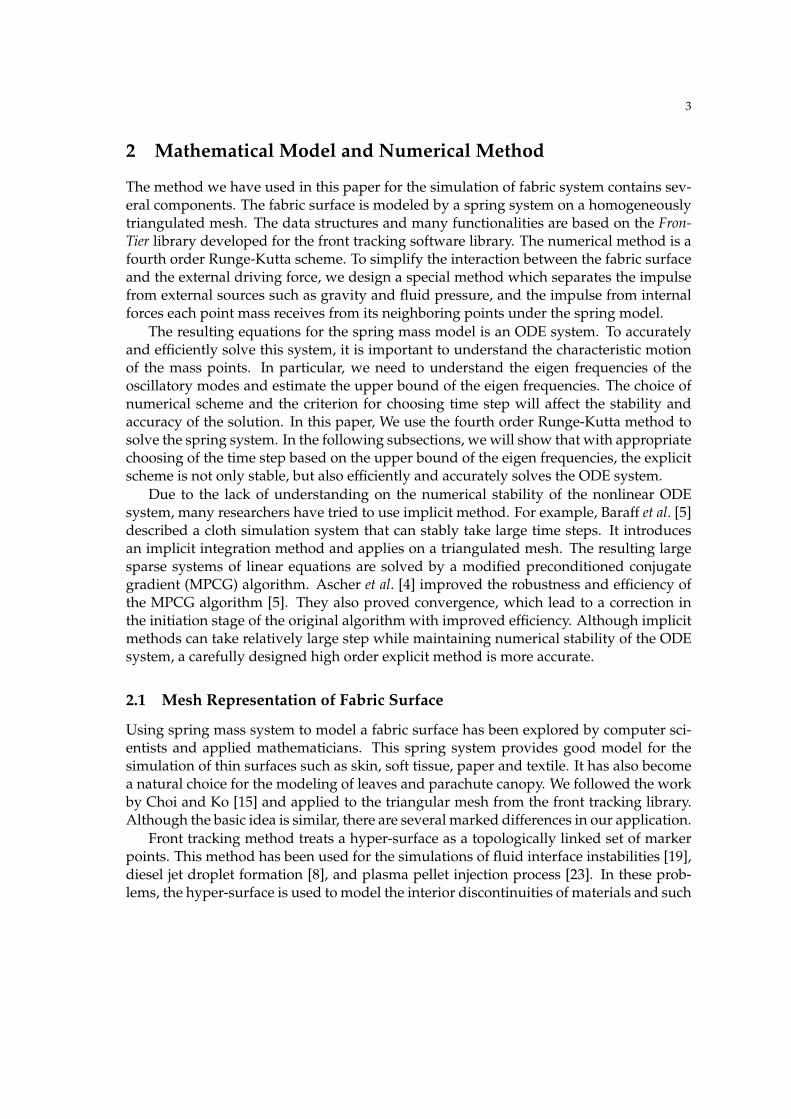
Figure 1: The spring model on a triangulated mesh. Each vertex point in the mesh rep-resents a mass point with point mass m. Each edge of the triangles has a equilibriumlength set during initialization and the changing length exerts a spring force on the twoneighboring vertices in opposite directions.
manifold surface may undergo complicated topological changes. Front tracking librarycontains data structure and functionalities to handle dynamic evolution of surface topol-ogy and to optimize hyper-surface mesh consistently. The basic data structure and manyfunctionalities are also used in our fabric modeling and simulation. The evolution offabric surface is simpler in topological handling due to the fact that a fabric surface canneither bifurcate nor merge. However the fabric system has certain constraints and posesnew challenges to the front tracking data structure and some associated functionalities.
The first new requirement is that the hyper-surface area must be conserved. Thisrequirement prompts us to add an equilibrium state of the mesh and treat the markerpoints of the hyper-surface as a set of spring vertices. The general property of a fabricsurface is that it is a non-stretchable surface. However, it is very difficult to numericallymaintain a meshed surface with constant area with non-deformable simplexes. Sincethere is always a finite elasticity of a fabric material, therefore to approximate the fabricsurface as a highly stiffened spring system is not only convenient, but also realistic. Oneof the major revision of the data structure is to add the equilibrium length for each sideof the simplexes (which are triangles for 3D hyper-surface). This variable is computed
5
after the initial mesh optimization and stored in memory throughout the computation.Figure 1 illustrates the spring model on the triangulated mesh using the front trackingdata structure.
The second difference between the material interface and the fabric surface lies inthe fact that the former is a manifold while the latter is an immersed surface. For themanifold surface, the positive and negative sides are not connected and can always berepresented as a level surface with positive and negative level function values on eachside. For an immersed surface, although one can still mark its positive and negativesides, such topological orientation is only local. A space point with short distance awayfrom the non-manifold surface cannot be classified as to which side of the hyper-surfaceit belongs. Such ambiguity poses difficulty in computing interpolation. We tackle thisproblem by using an index coating method. This method allows us to distinguish whichside a space point belongs to on the local basis (a few mesh blocks away from the surface).
Front tracking method also relies on the index of the side to check the topologicalconsistency of the interface. For an immersed interface, there is no topological bifurca-tion, but there will still be collision of the hyper-surface mesh points. Therefore, newfunctions to detect and resolve the marker point collision are needed, especially whenthe fabric surface is folded. In addition, the steady mesh triangulation throughout thecomputation makes the global indexing of vertices and triangles relatively easy to imple-ment. Such global indexing makes parallel partition and communication more accurateand robust.
2.2 Spring Models
When no external driving force is applied, the fabric surface, which is represented bythe spring mass system, is a conservative system whose total energy (kinetic energy pluspotential energy) is a constant. Assuming each mesh point represents a point mass min the spring system with position vector xi, the kinetic energy of the point mass i isTi = 1
2 m|xi|2, where xi is the time derivative, or velocity vector of the point mass i.We consider two types of spring systems. The first one, which we will refer to as
Model-I, has the potential energy between two point masses xi and xj in the form of
Vij =k2
∣∣(xi−xj)−(xi0−xj0)∣∣2 , (2.1)
where k is the spring constant and xi0 is the equilibrium position of mass point i. Thispotential energy does not match the properties of fabric, but it is easy to analyze. We canshow that a spring system with potential energy Eq. (2.1) has pure oscillatory motion andits eigen frequencies have an upper bound
√2Mk/m, where M is the maximum number
of neighbors a mass point can have. This upper bound of eigen frequencies plays animportant role in the analysis of numerical stability and accuracy for schemes to solvethe system.
6
As we mentioned in the introduction section, a fabric surface is considered as a mem-brane which is an idealized two dimensional manifold for which forces needed to bend itare negligible. Therefore at current stage we do not consider the bending energy. Model-I contains strong bending force and is not suitable for fabric modeling. For a realisticspring system to model the fabric surface, we have to assume that the spring force be-tween two neighboring mass points is only proportional to the displacement from theirequilibrium distance, the potential energy due to the relative displacement between twoneighboring point mass xi and xj is given by
Vij =k2(|xi−xj|−l0
ij)2, (2.2)
where l0ij = |xi0−xj0| is the equilibrium length between the two point masses. Here we
have made a modification from the model used by Choi and Ko in that we allow bothcontraction and expansion forces while in Choi and Ko’s equation, no force is applied if|xi−xj|< l0
ij. Choi and Ko’s choice does not conserve energy and would allow a surfaceshrink to a point without resistance. Such shrinking is unrealistic for a fabric surface. Wecall this system as Model-II.
The Lagrangians of the two systems are, therefore,
L=T−V =N
∑i=1
12
m|xi|2−14
N
∑i=1
N
∑j=1
k∣∣(xi−xj)−(xi0−xj0)
∣∣2 ηij (2.3)
for Model-I and
L=T−V =N
∑i=1
12
m|xi|2−14
N
∑i=1
N
∑j=1
k(|xi−xj|−l0ij)
2ηij (2.4)
for Model-II, where ηij is the adjacency coefficient between mass point i and j, and ηij =1if mass points i and j are immediate neighbors, ηij =0 if i= j or mass points i and j are notdirect neighbors.
Apply Lagrangian equationddt
(∂L∂qi
)=
∂L∂qi
to each mass point at xi, we have
mdxi
dt=m
d2xi
dt2 =−N
∑j=1
ηijk((xi−xj)−(xi0−xj0)
), (2.5)
for Model-I and
mdxi
dt=m
d2xi
dt2 =−N
∑j=1
ηijk(
xi−xj−l0ijeij
), (2.6)
for Model-II, where eij =xi−xj|xi−xj| is the unit vector from xi to xj.
7
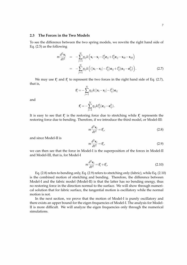
2.3 The Forces in the Two Models
To see the difference between the two spring models, we rewrite the right hand side ofEq. (2.5) as the following
md2xi
dt2 = −N
∑j=1
ηijk(
xi−xj−l0ijeij+l0
ijeij−xi0−xj0
)= −
N
∑j=1
ηijk((|xi−xj|−l0
ij)eij+l0ij(eij−e0
ij))
. (2.7)
We may use fsi and fr
i to represent the two forces in the right hand side of Eq. (2.7),that is,
fsi =−
N
∑j=1
ηijk(|xi−xj|−l0ij)eij
and
fri =−
N
∑j=1
ηijkl0ij(eij−e0
ij).
It is easy to see that fsi is the restoring force due to stretching while fr
i represents therestoring force due to bending. Therefore, if we introduce the third model, or Model-III:
md2xi
dt2 = fri , (2.8)
and since Model-II is
md2xi
dt2 = fsi , (2.9)
we can then see that the force in Model-I is the superposition of the forces in Model-IIand Model-III, that is, for Model-I
md2xi
dt2 = fsi +fr
i , (2.10)
Eq. (2.8) refers to bending only, Eq. (2.9) refers to stretching only (fabric), while Eq. (2.10)is the combined motion of stretching and bending. Therefore, the difference betweenModel-I and the fabric model (Model-II) is that the latter has no bending energy, thusno restoring force in the direction normal to the surface. We will show through numeri-cal solution that for fabric surface, the tangential motion is oscillatory while the normalmotion is not.
In the next section, we prove that the motion of Model-I is purely oscillatory andthere exists an upper bound for the eigen frequencies of Model-I. The analysis for Model-II is more difficult. We will analyze the eigen frequencies only through the numericalsimulations.
8
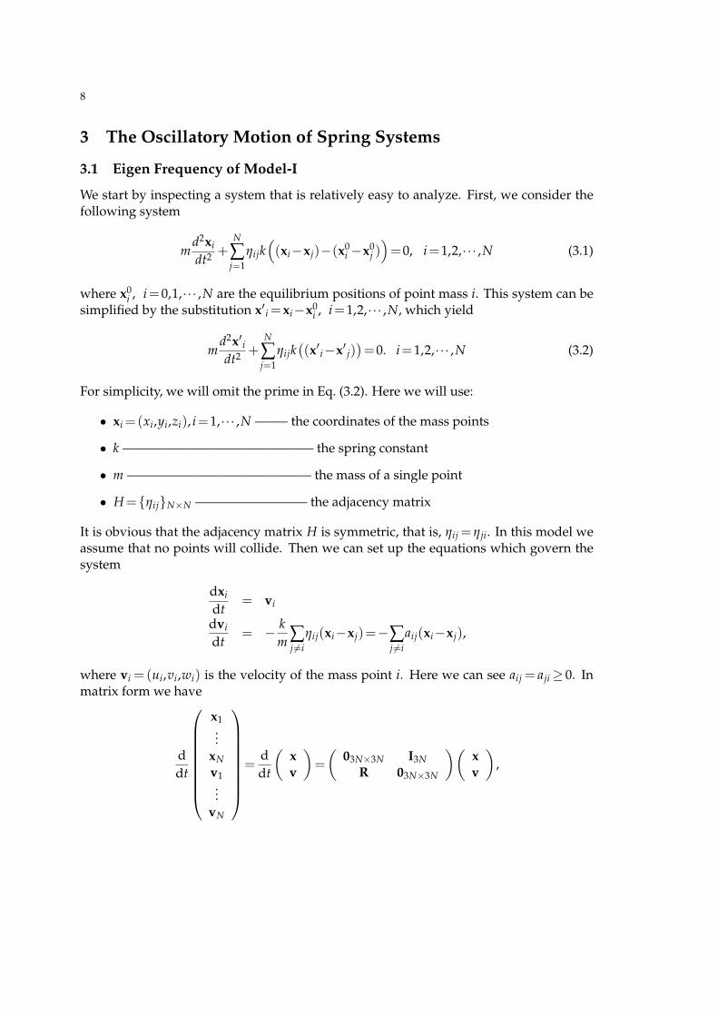
3 The Oscillatory Motion of Spring Systems
3.1 Eigen Frequency of Model-I
We start by inspecting a system that is relatively easy to analyze. First, we consider thefollowing system
md2xi
dt2 +N
∑j=1
ηijk((xi−xj)−(x0
i −x0j ))
=0, i=1,2,··· ,N (3.1)
where x0i , i =0,1,··· ,N are the equilibrium positions of point mass i. This system can be
simplified by the substitution x′i =xi−x0i , i=1,2,··· ,N, which yield
md2x′idt2 +
N
∑j=1
ηijk((x′i−x′ j)
)=0. i=1,2,··· ,N (3.2)
For simplicity, we will omit the prime in Eq. (3.2). Here we will use:
• xi =(xi,yi,zi), i=1,··· ,N ——– the coordinates of the mass points
• k ——————————————– the spring constant
• m —————————————— the mass of a single point
• H ={ηij}N×N ————————– the adjacency matrix
It is obvious that the adjacency matrix H is symmetric, that is, ηij =ηji. In this model weassume that no points will collide. Then we can set up the equations which govern thesystem
dxi
dt= vi
dvi
dt= − k
m ∑j 6=i
ηij(xi−xj)=−∑j 6=i
aij(xi−xj),
where vi =(ui,vi,wi) is the velocity of the mass point i. Here we can see aij = aji≥ 0. Inmatrix form we have
ddt
x1...
xNv1...
vN
=
ddt
(xv
)=(
03N×3N I3NR 03N×3N
)(xv
),
9
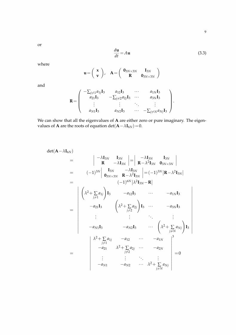
ordudt
= Au (3.3)
where
u=(
xv
), A=
(03N×3N I3N
R 03N×3N
)and
R=
−∑j 6=1 a1jI3 a12I3 ··· a1NI3
a21I3 −∑j 6=2 a2jI3 ··· a3NI3...
.... . .
...aN1I3 aN2I3 ··· −∑j 6=N aNjI3
.
We can show that all the eigenvalues of A are either zero or pure imaginary. The eigen-values of A are the roots of equation det(A−λI6N)=0.
det(A−λI6N)
=∣∣∣∣ −λI3N I3N
R −λI3N
∣∣∣∣= ∣∣∣∣ −λI3N I3NR−λ2I3N 03N×3N
∣∣∣∣= (−1)3N
∣∣∣∣ I3N −λI3N03N×3N R−λ2I3N
∣∣∣∣=(−1)3N∣∣R−λ2I3N
∣∣= (−1)6N
∣∣λ2I3N−R∣∣
=
∣∣∣∣∣∣∣∣∣∣∣∣∣∣∣∣∣∣
(λ2+ ∑
j 6=1a1j
)I3 −a12I3 ··· −a1NI3
−a21I3
(λ2+ ∑
j 6=2a2j
)I3 ··· −a3NI3
......
. . ....
−aN1I3 −aN2I3 ···(
λ2+ ∑j 6=N
aNj
)I3
∣∣∣∣∣∣∣∣∣∣∣∣∣∣∣∣∣∣
=
∣∣∣∣∣∣∣∣∣∣∣∣∣
λ2+ ∑j 6=1
a1j −a12 ··· −a1N
−a21 λ2+ ∑j 6=2
a2j ··· −a2N
......
. . ....
−aN1 −aN2 ··· λ2+ ∑j 6=N
aNj
∣∣∣∣∣∣∣∣∣∣∣∣∣
3
=0
10
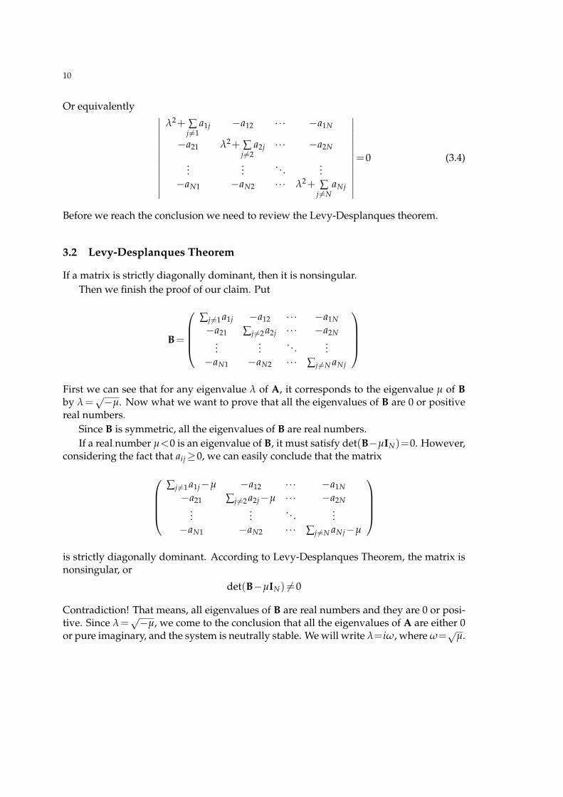
Or equivalently ∣∣∣∣∣∣∣∣∣∣∣∣∣
λ2+ ∑j 6=1
a1j −a12 ··· −a1N
−a21 λ2+ ∑j 6=2
a2j ··· −a2N
......
. . ....
−aN1 −aN2 ··· λ2+ ∑j 6=N
aNj
∣∣∣∣∣∣∣∣∣∣∣∣∣=0 (3.4)
Before we reach the conclusion we need to review the Levy-Desplanques theorem.
3.2 Levy-Desplanques Theorem
If a matrix is strictly diagonally dominant, then it is nonsingular.Then we finish the proof of our claim. Put
B=
∑j 6=1 a1j −a12 ··· −a1N
−a21 ∑j 6=2 a2j ··· −a2N...
.... . .
...−aN1 −aN2 ··· ∑j 6=N aNj
First we can see that for any eigenvalue λ of A, it corresponds to the eigenvalue µ of Bby λ =
√−µ. Now what we want to prove that all the eigenvalues of B are 0 or positivereal numbers.
Since B is symmetric, all the eigenvalues of B are real numbers.If a real number µ<0 is an eigenvalue of B, it must satisfy det(B−µIN)=0. However,
considering the fact that aij≥0, we can easily conclude that the matrix
∑j 6=1 a1j−µ −a12 ··· −a1N
−a21 ∑j 6=2 a2j−µ ··· −a2N...
.... . .
...−aN1 −aN2 ··· ∑j 6=N aNj−µ
is strictly diagonally dominant. According to Levy-Desplanques Theorem, the matrix isnonsingular, or
det(B−µIN) 6=0
Contradiction! That means, all eigenvalues of B are real numbers and they are 0 or posi-tive. Since λ=
√−µ, we come to the conclusion that all the eigenvalues of A are either 0or pure imaginary, and the system is neutrally stable. We will write λ=iω, where ω=√µ.
11
3.3 Bound of Eigen Values of Model-I
Assume that every mass point has at most M neighbors, and that the displacement ofall points do not vary too much, we can estimate the upper bound of the eigenvalues byestimating that of matrix B. According to Gershgorin circle theorem, all the eigenvaluesof B lie within the circles Di,i=1,··· ,N where
Di ={µ;
∣∣∣∣∣µ−(−∑j 6=i
aij)
∣∣∣∣∣≤∑j 6=i
aij}.
Then we can see
|µ|≤2
∣∣∣∣∣∑j 6=iaij
∣∣∣∣∣≈2Ma=2Mk
m. (3.5)
In other words, all the eigenvalues of A satisfy
|λ|=√|µ|≤
√2Mk
m. (3.6)
The numerical experiments show that this upper bound is actually a little too high. Thenumerical solutions suggest that the minimum upper bound should be
ω = |λ|=√|µ|≤
√Mkm
. (3.7)
3.4 Oscillatory Motion of Model-II
To analyze Model-II, we rewrite the Eq. (2.6) as the following
mdxi
dt=−
N
∑j=1
ηijk(
xi−xj−l0ijeij
)=−
N
∑j=1
ηijk∆lijlij
(xi−xj
), (3.8)
where lij=|xi−xj| and ∆lij=lij−l0ij. Since ∆lij can be either positive or negative, we cannot
guarantee that all the eigen values of the system are imaginary.We write Eq. (2.6) as
md2xi
dt2 =−∑j 6=i
aij(lij)(xi−xj), (3.9)
where
aij =ηijk
(1−
l0ij
lij
).
We linearize Eq. (3.9) and obtain
md2δxi
dt2 = −∑j 6=i
{δaij(lij)(xi−xj)+aij(δxi−δxj)
}(3.10)
12
Using
δaij(lij)= a′(lij)δlij =ηijkl0ij
l2ij
δlij
and
δlij = δ
(∑d
(xdi −xd
j )2
)1/2
=∑d(xd
i −xdj )(δxd
i −δxdj )(
∑d(xdi −xd
j )2)1/2 =
1lij
(xi−xj)·(δxi−δxj),
we obtain
δaij(xi−xj) = ηijk
[l0ij
l3ij(xi−xj)
((xi−xj)·(δxi−δxj)
)]
= ηijk
[l0ij
lijeij(eij ·(δxi−δxj)
)]
= ηijk
[l0ij
lijeij⊗eij(δxi−δxj)
].
(3.11)
Substituting Eq. (3.11) into Eq. (3.10), we have
md2δxi
dt2 =−∑j 6=i
ηijk
(l0ij
lijeij⊗eij+
(1−
l0ij
lij
)I
)(δxi−δxj) (3.12)
The summation on right hand side of Eq. (3.12) represents the superposition of forces dueto each neighboring mass point. Using eij to make dot product for each term, we obtainthe tangential component of acceleration
f tij = −eij ·ηijk
(l0ij
lijeij⊗eij+
(1−
l0ij
lij
)I
)(δxi−δxj)
= −ηijk(eij ·(δxi−δxj)
)(3.13)
Eq. (3.13) indicates that the force on a mass point along each direction to its neighbors isrestoring, therefore the motion is oscillatory.
13
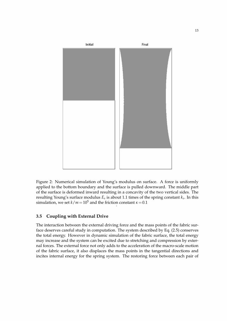
Figure 2: Numerical simulation of Young’s modulus on surface. A force is uniformlyapplied to the bottom boundary and the surface is pulled downward. The middle partof the surface is deformed inward resulting in a concavity of the two vertical sides. Theresulting Young’s surface modulus Es is about 1.1 times of the spring constant ks. In thissimulation, we set k/m=105 and the friction constant κ =0.1.
3.5 Coupling with External Drive
The interaction between the external driving force and the mass points of the fabric sur-face deserves careful study in computation. The system described by Eq. (2.5) conservesthe total energy. However in dynamic simulation of the fabric surface, the total energymay increase and the system can be excited due to stretching and compression by exter-nal forces. The external force not only adds to the acceleration of the macro-scale motionof the fabric surface, it also displaces the mass points in the tangential directions andincites internal energy for the spring system. The restoring force between each pair of
14
neighboring mass points of the spring system serves as the self-adjustment to satisfy thefabric constraint and Young’s modulus. However, when the internal energy of the springsystem is too high, the system may be dominated by the random meso-scale motion ofthe mass points. Therefore adding a damping force will help to stabilize the system.
When there is an external velocity field ve, we define the external impulse as Iei =mve
i ,where ve
i is the external driving velocity at point xi. At any given time, we can solve theequations of the spring system and obtain the internal impulse Is
i . Since the spring forceis a function of the relative position of the point mass with respect to its neighbors, wecan use the superposition principle and add to the total impulse
Ii = Iei +Is
i . (3.14)
Our method is to apply damping to the internal impulse only.In a fluid interaction, the fabric surface points may be driven by three forces, the grav-
itational force due to the weight of the fabric surface point masses, the pressure force fromthe surrounding fluid, and the internal force, or the spring restoring force and friction (toprevent the spring system becoming over excited). We separate the impulse on a masspoint into three components, the gravitational impulse, the pressure force impulse andthe internal impulse due to neighboring point mass in the spring system, that is
Ii = Igi +Ip
i +Isi . (3.15)
The interaction between the fabric surface and fluid is through the normal componentof the force on each mass point. At every time step, the fluid exerts an impulse to themass points, but this part of the impulse is balanced by the gravitational impulse and therestoring force of the spring. The normal component of the superposition of the threeforces feeds back to the fluid in the following step. The result is that the momentumexchange between the fabric surface and the fluid is equal in magnitude and opposite indirections, a requirement by Newton’s third law.
To prevent the spring system getting into over-excited state, we add a damping forceto the system. Therefore, the complete system of equations is the following
dvi
dt= − 1
m
N
∑j=1
ηijk(|xi−xj|−l0
ij
)eij+fe
i−κvsi ,
dxi
dt= vi,
where fei is the external force, κ is the damping coefficient and vs
i is the velocity compo-nent due to the spring impulse vs
i = Isi /m.
3.6 Collision Handling
Collision handling is a challenging work to many researchers in fabric modeling. Re-cently many authors have presented their algorithms and techniques on this tedious but
15
important work. Bez et al. [7] introduced the topological mapping approach to collisiondetection for the drape simulation work. Bridson et al. [11, 12] presented an algorithmto efficiently and robustly process collisions, contact and friction in cloth simulation.Bargmann [6] presented a new approach to collision detection and collision response ofcloth onto deformable volumes, along with a self-collision algorithm to handle collisionsof the cloth with itself.
Our FronTier library has a set of functions for detection of collisions, although theexisting functions were designed to resolve collisions through topological bifurcation ormerging using the locally grid based method [16]. For the modeling of fabric surface,we modify the functions to reflecting the colliding marker points in the normal directionof the surface. The detection uses an efficient hashing method and is of order O(nN),where n is the number of triangles hashed by one grid block and N is the total number oftriangles.
3.7 Numerical Stability of the Spring System
The spring system is an energy conservative ODE system if we set the damping coeffi-cient equal to zero. The numerical methods for solving system of ordinary differentialequations is now a curriculum topic in numerical analysis courses. Although textbookssuch as the one by Butcher [13] discussed method for the oscillatory linear system, fewhave mentioned about the crucial role of the upper bound of the eigen frequency in thestability and accuracy analysis for the conservative ODE system. In this section, we givea detailed derivation of the truncation error of the Runge-Kutta methods and their de-pendency on the frequency of the oscillation.
In one dimension or for Model-I (Eq. (2.5)), the equations of spring system can betransformed into homogeneous equation if we redefine xi as the relative displacementfrom its equilibrium position. Therefore, we will first consider the numerical stability ofEq. (3.3)
dudt
= Au,
here we have used u = {xT1 ,xT
2 ,··· ,xTN ,vT
1 ,vT2 ,··· ,vT
N}T. If we can diagonalize the matrixA=T−1ΛT, and introduce w=Tu, we can obtain the decoupled equation
dwdt
=Λw (3.16)
Therefore to consider the stability of the system Eq. (3.16), we should consider the scalarequation
dydt
=λy. (3.17)
The Euler method for Eq. (3.17)
yn+1 =yn(1+λ∆t) (3.18)
16
and its stability is well known if λ is real. However, for a conservative system like thespring equations with damping coefficient equal to zero, all the eigen values of A areimaginary. Therefore, we will need to consider the following equation
dydt
= iωy, (3.19)
with ω = |λ|=√µ. If we use the Euler forward method for Eq. (3.19), that is
yn+1 =yn(1+iω∆t), (3.20)
since the square mode of the recursive factor χ2= |1+iω∆t|2=1+ω2∆t2>1, therefore thesolution will be amplified after each time step by χ. To reduce this unphysical amplifica-tion, we need to make ω∆t�1 by reducing ∆t.
With same ∆t, an increasing order of the scheme will reduce this amplification factoreffectively. For the second order predictor-corrector method
y∗= yn(1+iω∆t)yn+1 = yn+ 1
2 iω∆t(yn+y∗)=(1− 1
2 ω2∆t2+iω∆t)
yn (3.21)
will have χ2 =1+ 14 (ω∆t)4. In particular, for the fourth order Runge-Kutta method, that
is
yn+1 = yn+∆t6
(K1+2K2+2K3+K4)
K1 = iωyn
K2 = iω(
yn+∆t2
K1
)= iωyn
(1+
iω∆t2
)K3 = iω
(yn+
∆t2
K2
)= iωyn
(1+
iω∆t2
+(iω∆t)2
4
)K4 = iω(yn+∆tK3)= iωyn
(1+iω∆t+
(iω∆t)2
2+
(iω∆t)3
4
)and we can see
yn+1 = yn+h6(K1+2K2+2K3+K4)
=(
1+iω∆t+(iω∆t)2
2+
(iω∆t)3
6+
(iω∆t)4
24
)yn.
=(
1+iω∆t− (ω∆t)2
2− i(ω∆t)3
6+
(ω∆t)4
24
)yn
=((
1− (ω∆t)2
2+
(ω∆t)4
24
)+i(
ω∆t− (ω∆t)3
6
))yn.
17
The growth factor is
χ2 =∣∣∣∣(1− (ω∆t)2
2+
(ω∆t)4
24
)+i(
ω∆t− (ω∆t)3
6
)∣∣∣∣2=
(1− (ω∆t)2
2+
(ω∆t)4
24
)2
+(
ω∆t− (ω∆t)3
6
)2
= 1− 172
(ω∆t)6+1
576(ω∆t)8. (3.22)
The above calculation shows that the fourth order Runge-Kutta method for the oscillatorysystem is not only stable, but also very accurate.
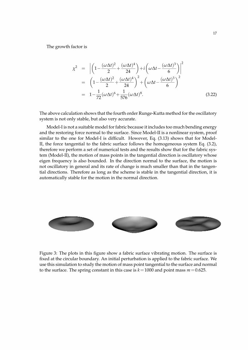
Model-I is not a suitable model for fabric because it includes too much bending energyand the restoring force normal to the surface. Since Model-II is a nonlinear system, proofsimilar to the one for Model-I is difficult. However, Eq. (3.13) shows that for Model-II, the force tangential to the fabric surface follows the homogeneous system Eq. (3.2),therefore we perform a set of numerical tests and the results show that for the fabric sys-tem (Model-II), the motion of mass points in the tangential direction is oscillatory whoseeigen frequency is also bounded. In the direction normal to the surface, the motion isnot oscillatory in general and its rate of change is much smaller than that in the tangen-tial directions. Therefore as long as the scheme is stable in the tangential direction, it isautomatically stable for the motion in the normal direction.
Figure 3: The plots in this figure show a fabric surface vibrating motion. The surface isfixed at the circular boundary. An initial perturbation is applied to the fabric surface. Weuse this simulation to study the motion of mass point tangential to the surface and normalto the surface. The spring constant in this case is k=1000 and point mass m=0.625.
18
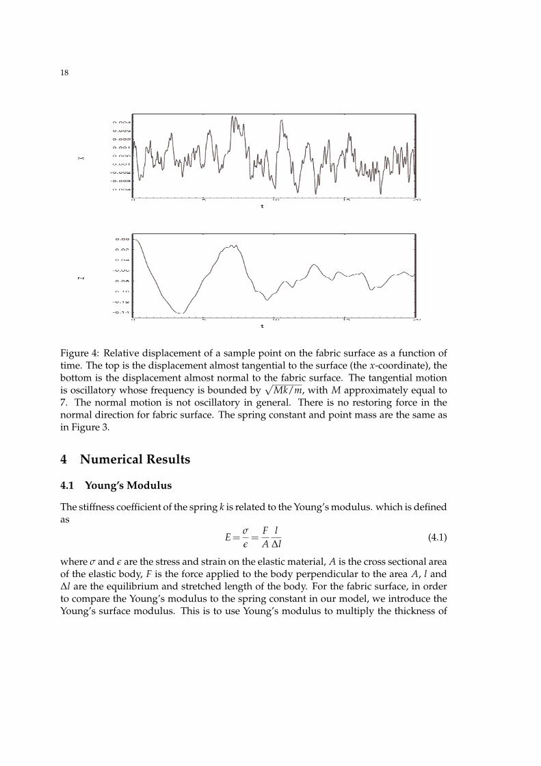
Figure 4: Relative displacement of a sample point on the fabric surface as a function oftime. The top is the displacement almost tangential to the surface (the x-coordinate), thebottom is the displacement almost normal to the fabric surface. The tangential motionis oscillatory whose frequency is bounded by
√Mk/m, with M approximately equal to
7. The normal motion is not oscillatory in general. There is no restoring force in thenormal direction for fabric surface. The spring constant and point mass are the same asin Figure 3.
4 Numerical Results
4.1 Young’s Modulus
The stiffness coefficient of the spring k is related to the Young’s modulus. which is definedas
E=σ
ε=
FA
l∆l
(4.1)
where σ and ε are the stress and strain on the elastic material, A is the cross sectional areaof the elastic body, F is the force applied to the body perpendicular to the area A, l and∆l are the equilibrium and stretched length of the body. For the fabric surface, in orderto compare the Young’s modulus to the spring constant in our model, we introduce theYoung’s surface modulus. This is to use Young’s modulus to multiply the thickness of
19
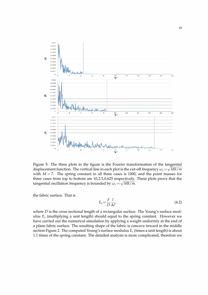
Figure 5: The three plots in the figure is the Fourier transformation of the tangentialdisplacement function. The vertical line in each plot is the cut-off frequency ωc=
√Mk/m
with M = 7. The spring constant in all three cases is 1000, and the point masses forthree cases from top to bottom are 10,2.5,0.625 respectively. These plots prove that thetangential oscillation frequency is bounded by ωc =
√Mk/m.
the fabric surface. That is
Es =FD
l∆l
, (4.2)
where D is the cross sectional length of a rectangular surface. The Young’s surface mod-ulus Es (multiplying a unit length) should equal to the spring constant. However wehave carried out the numerical simulation by applying a weight uniformly at the end ofa plane fabric surface. The resulting shape of the fabric is concave inward in the middlesection Figure 2. The computed Young’s surface modulus Es (times a unit length) is about1.1 times of the spring constant. The detailed analysis is more complicated, therefore we
20
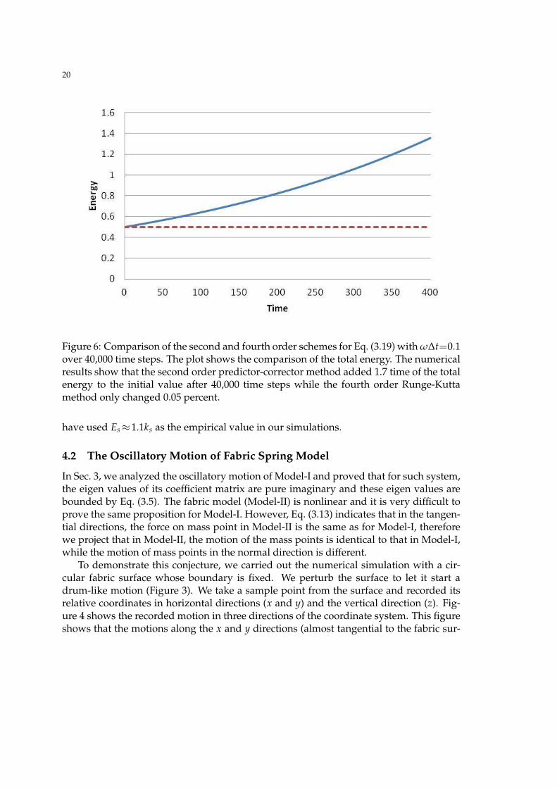
Figure 6: Comparison of the second and fourth order schemes for Eq. (3.19) with ω∆t=0.1over 40,000 time steps. The plot shows the comparison of the total energy. The numericalresults show that the second order predictor-corrector method added 1.7 time of the totalenergy to the initial value after 40,000 time steps while the fourth order Runge-Kuttamethod only changed 0.05 percent.
have used Es≈1.1ks as the empirical value in our simulations.
4.2 The Oscillatory Motion of Fabric Spring Model
In Sec. 3, we analyzed the oscillatory motion of Model-I and proved that for such system,the eigen values of its coefficient matrix are pure imaginary and these eigen values arebounded by Eq. (3.5). The fabric model (Model-II) is nonlinear and it is very difficult toprove the same proposition for Model-I. However, Eq. (3.13) indicates that in the tangen-tial directions, the force on mass point in Model-II is the same as for Model-I, thereforewe project that in Model-II, the motion of the mass points is identical to that in Model-I,while the motion of mass points in the normal direction is different.
To demonstrate this conjecture, we carried out the numerical simulation with a cir-cular fabric surface whose boundary is fixed. We perturb the surface to let it start adrum-like motion (Figure 3). We take a sample point from the surface and recorded itsrelative coordinates in horizontal directions (x and y) and the vertical direction (z). Fig-ure 4 shows the recorded motion in three directions of the coordinate system. This figureshows that the motions along the x and y directions (almost tangential to the fabric sur-
21
Order of Scheme N=400 N=4000 N=40000First Order 52.5 9.6×10¹⁶ ∞
Second Order 0.01 0.105 1.7Fourth Order −6.0×10⁻⁶ −5.6×10⁻⁵ −5.5×10⁻⁴
Table 1: Comparison of numerical schemes for ODE Eq. (3.19) with ω∆t = 0.1 over 400,4000, and 40000 steps respectively. The values in the table are for ∆E
E0, where E0 is the total
energy at t = 0, and ∆E = E(T)−E0 is the difference between the final total energy theinitial total energy.
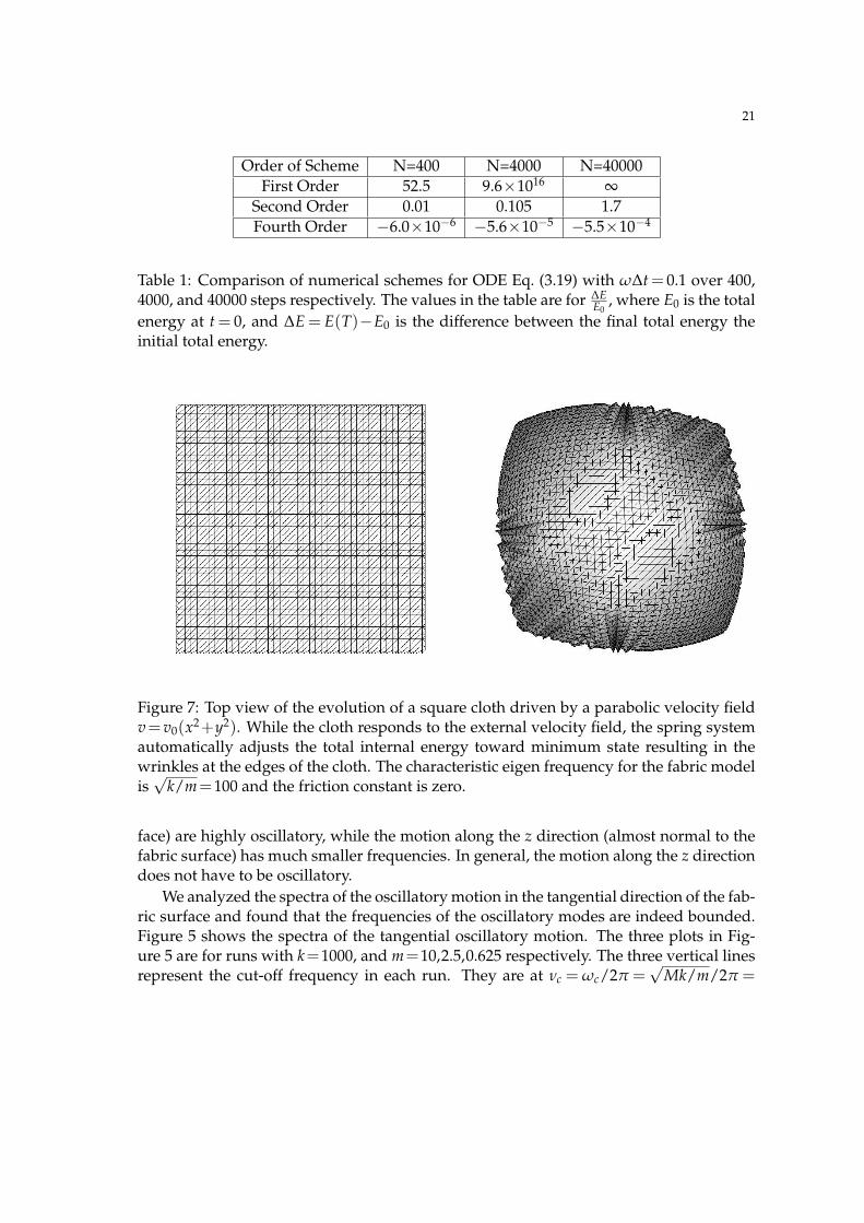
Figure 7: Top view of the evolution of a square cloth driven by a parabolic velocity fieldv = v0(x2+y2). While the cloth responds to the external velocity field, the spring systemautomatically adjusts the total internal energy toward minimum state resulting in thewrinkles at the edges of the cloth. The characteristic eigen frequency for the fabric modelis√
k/m=100 and the friction constant is zero.
face) are highly oscillatory, while the motion along the z direction (almost normal to thefabric surface) has much smaller frequencies. In general, the motion along the z directiondoes not have to be oscillatory.
We analyzed the spectra of the oscillatory motion in the tangential direction of the fab-ric surface and found that the frequencies of the oscillatory modes are indeed bounded.Figure 5 shows the spectra of the tangential oscillatory motion. The three plots in Fig-ure 5 are for runs with k=1000, and m=10,2.5,0.625 respectively. The three vertical linesrepresent the cut-off frequency in each run. They are at νc = ωc/2π =
√Mk/m/2π =
22
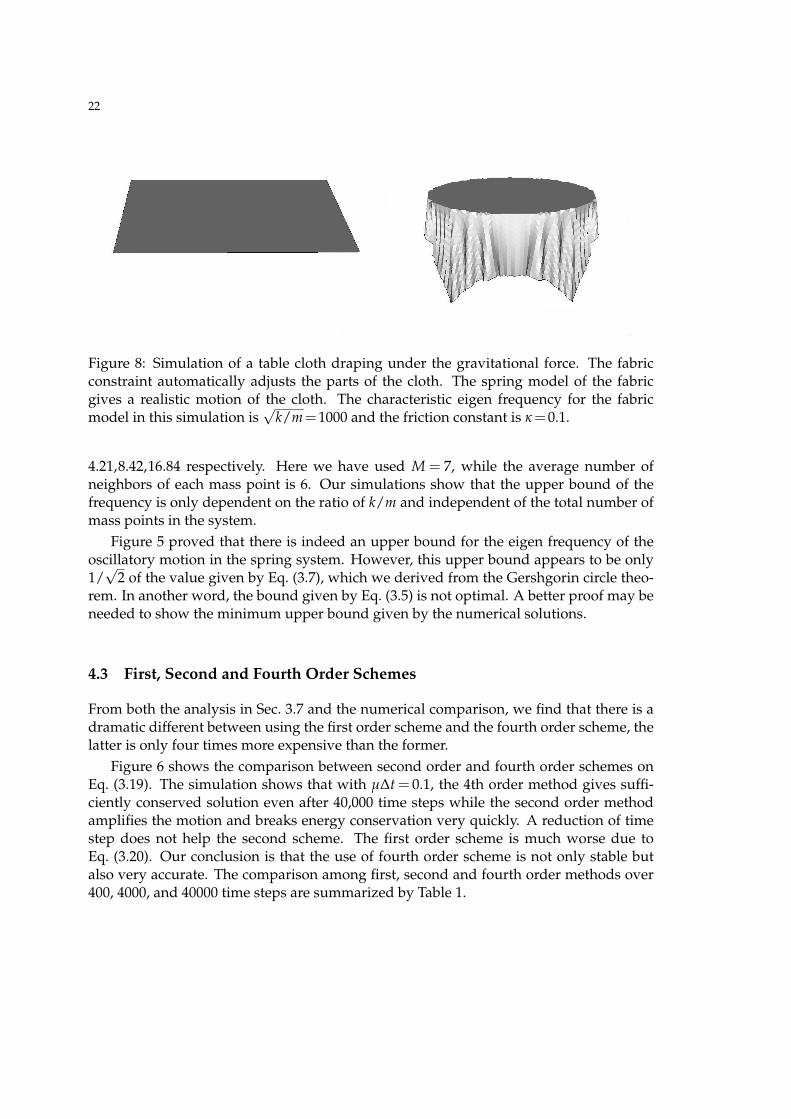
Figure 8: Simulation of a table cloth draping under the gravitational force. The fabricconstraint automatically adjusts the parts of the cloth. The spring model of the fabricgives a realistic motion of the cloth. The characteristic eigen frequency for the fabricmodel in this simulation is
√k/m=1000 and the friction constant is κ =0.1.
4.21,8.42,16.84 respectively. Here we have used M = 7, while the average number ofneighbors of each mass point is 6. Our simulations show that the upper bound of thefrequency is only dependent on the ratio of k/m and independent of the total number ofmass points in the system.
Figure 5 proved that there is indeed an upper bound for the eigen frequency of theoscillatory motion in the spring system. However, this upper bound appears to be only1/√
2 of the value given by Eq. (3.7), which we derived from the Gershgorin circle theo-rem. In another word, the bound given by Eq. (3.5) is not optimal. A better proof may beneeded to show the minimum upper bound given by the numerical solutions.
4.3 First, Second and Fourth Order Schemes
From both the analysis in Sec. 3.7 and the numerical comparison, we find that there is adramatic different between using the first order scheme and the fourth order scheme, thelatter is only four times more expensive than the former.
Figure 6 shows the comparison between second order and fourth order schemes onEq. (3.19). The simulation shows that with µ∆t = 0.1, the 4th order method gives suffi-ciently conserved solution even after 40,000 time steps while the second order methodamplifies the motion and breaks energy conservation very quickly. A reduction of timestep does not help the second scheme. The first order scheme is much worse due toEq. (3.20). Our conclusion is that the use of fourth order scheme is not only stable butalso very accurate. The comparison among first, second and fourth order methods over400, 4000, and 40000 time steps are summarized by Table 1.
23
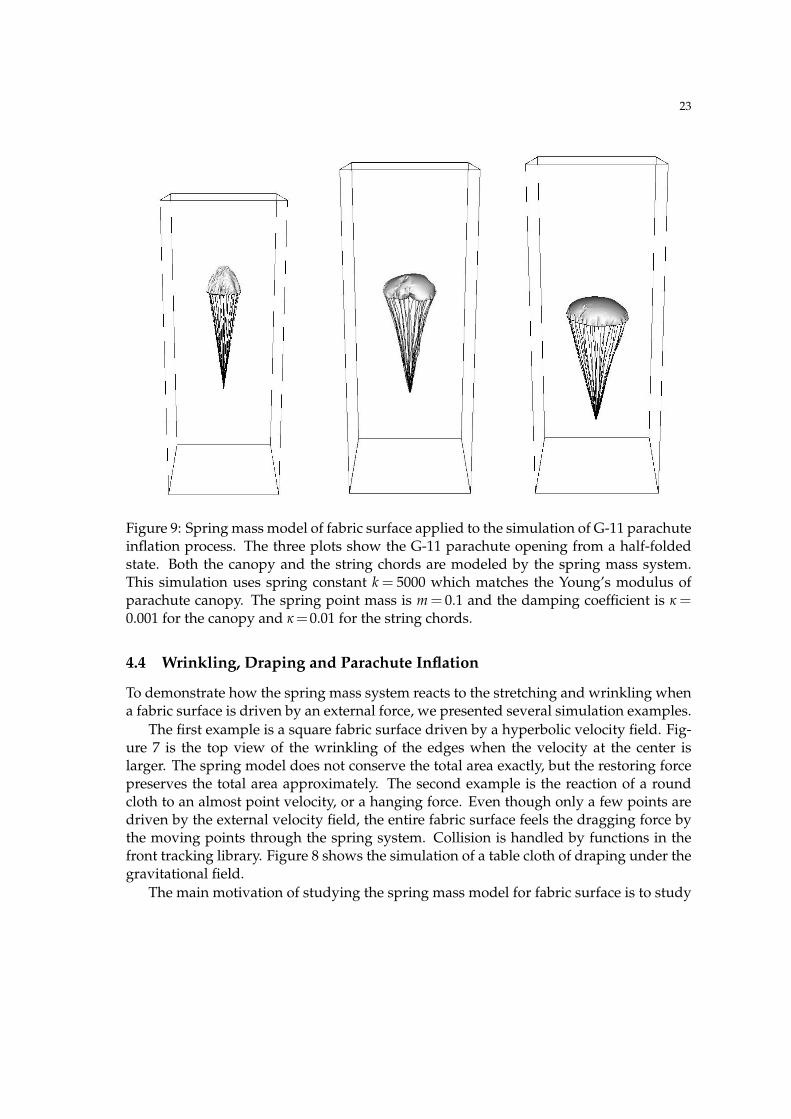
Figure 9: Spring mass model of fabric surface applied to the simulation of G-11 parachuteinflation process. The three plots show the G-11 parachute opening from a half-foldedstate. Both the canopy and the string chords are modeled by the spring mass system.This simulation uses spring constant k = 5000 which matches the Young’s modulus ofparachute canopy. The spring point mass is m = 0.1 and the damping coefficient is κ =0.001 for the canopy and κ =0.01 for the string chords.
4.4 Wrinkling, Draping and Parachute Inflation
To demonstrate how the spring mass system reacts to the stretching and wrinkling whena fabric surface is driven by an external force, we presented several simulation examples.
The first example is a square fabric surface driven by a hyperbolic velocity field. Fig-ure 7 is the top view of the wrinkling of the edges when the velocity at the center islarger. The spring model does not conserve the total area exactly, but the restoring forcepreserves the total area approximately. The second example is the reaction of a roundcloth to an almost point velocity, or a hanging force. Even though only a few points aredriven by the external velocity field, the entire fabric surface feels the dragging force bythe moving points through the spring system. Collision is handled by functions in thefront tracking library. Figure 8 shows the simulation of a table cloth of draping under thegravitational field.
The main motivation of studying the spring mass model for fabric surface is to study
24
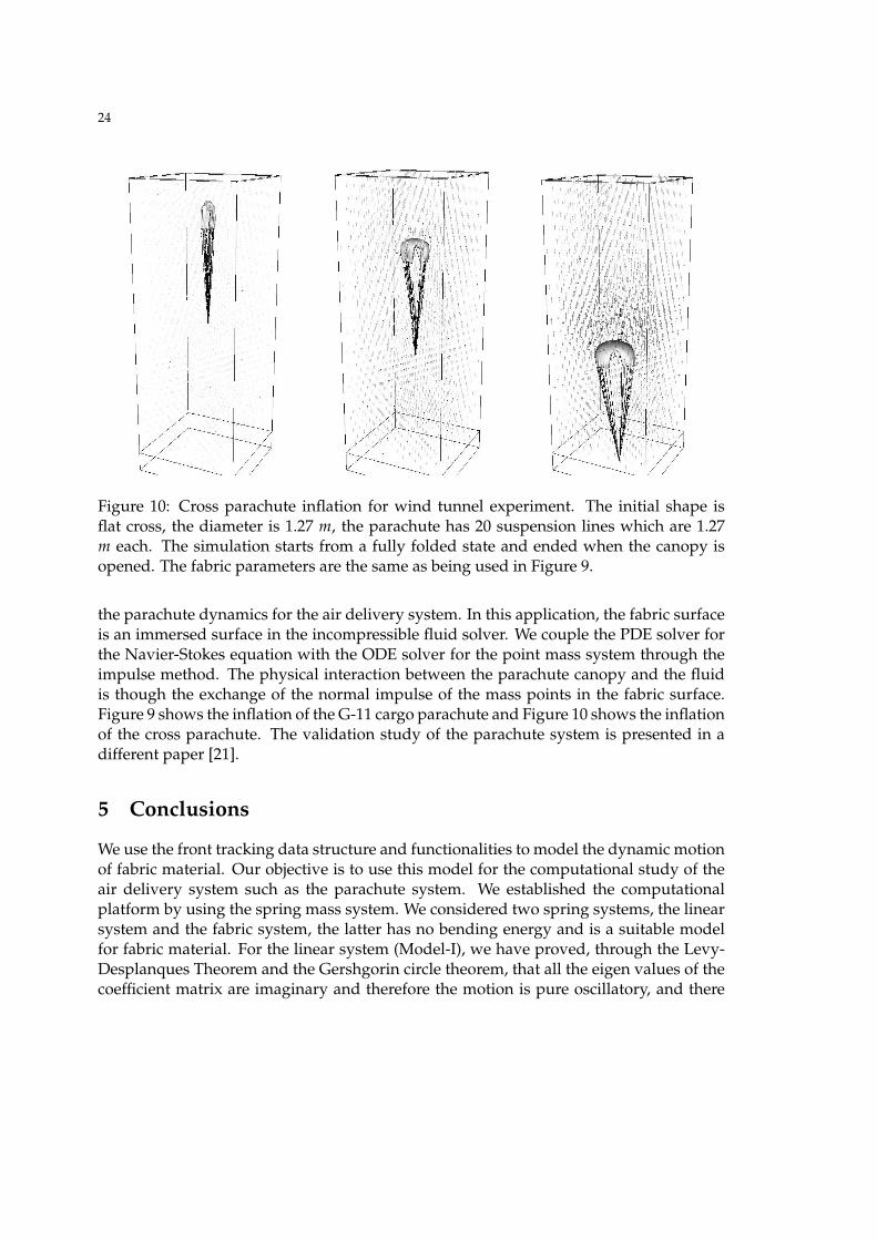
Figure 10: Cross parachute inflation for wind tunnel experiment. The initial shape isflat cross, the diameter is 1.27 m, the parachute has 20 suspension lines which are 1.27m each. The simulation starts from a fully folded state and ended when the canopy isopened. The fabric parameters are the same as being used in Figure 9.
the parachute dynamics for the air delivery system. In this application, the fabric surfaceis an immersed surface in the incompressible fluid solver. We couple the PDE solver forthe Navier-Stokes equation with the ODE solver for the point mass system through theimpulse method. The physical interaction between the parachute canopy and the fluidis though the exchange of the normal impulse of the mass points in the fabric surface.Figure 9 shows the inflation of the G-11 cargo parachute and Figure 10 shows the inflationof the cross parachute. The validation study of the parachute system is presented in adifferent paper [21].
5 Conclusions
We use the front tracking data structure and functionalities to model the dynamic motionof fabric material. Our objective is to use this model for the computational study of theair delivery system such as the parachute system. We established the computationalplatform by using the spring mass system. We considered two spring systems, the linearsystem and the fabric system, the latter has no bending energy and is a suitable modelfor fabric material. For the linear system (Model-I), we have proved, through the Levy-Desplanques Theorem and the Gershgorin circle theorem, that all the eigen values of thecoefficient matrix are imaginary and therefore the motion is pure oscillatory, and there
25
exists an upper bound |µ|≤√
2Mk/m, where M is the maximum number of neighbors aspring mass point can have.
The nonlinear spring model is more difficult to analyze. But we found that the forcealong the direction to the neighbors of a vertex is the same as in the linear model. Nu-merically, we have showed that indeed, the motion of a spring mass point is oscillatoryalong the tangential direction of the fabric surface. The motion in the direction normalto the surface is not oscillatory in general. Fourier analysis of the tangential motion onan arbitrary sample point showed that the frequency of the oscillation is bounded by√
Mk/m/2π, where M≈7.For the oscillatory motion, the first order Euler forward scheme for the ODE system
is increasing in amplitude. Higher order Runge-Kutta scheme is a much efficient way tosolve the equations. Our computation showed that the fourth order Runge-Kutta schemewith µmax∆t≤0.1 gives very stable and accurate solution to the spring mass ODE system.
There are still two open problems. The first is that although the analysis of Model-Ithrough the Gershgorin circle theorem gives an upper bound of the eigen frequency asωc≤
√2Mk/m, our numerical tests suggest that this upper bound is not a sharp bound.
The minimum bound appears to be ωc≤√
Mk/m. The second is that we still need theanalytical proof of the upper bound for the nonlinear system of Model-II.
6 Acknowledgement
The authors would like to acknowledge many discussions with Xiangmin Jiao and Keh-Ming Shyue. Joungdong Kim and Xiaolin Li are supported in part by the US Army Re-search Office under the ARO grant award W911NF0910306. Xiaolin Li would like tothank the Department of Mathematics, National Taiwan University and to acknowledgethe generous support from National Science Council of The Republic of China, GrantNSC 101-2811-M-002-006 on his sabbatical visit during which this work is accomplished.
References
[1] R. Fedkiw A. Selle, M. Lentine. A mass spring model for hair simulation. ACM Transactionson Graphics (Proceedings of the ACM SIGGRAPH’08 conference), 27, 2008.
[2] M. Aono, D. Breen, and M. Wozny. Fitting a woven cloth model to a curved surface: map-ping algorithms. Computer-Aided Design, 26(4):278–292, April 1994.
[3] M. Aono, P. Denti, D. Breen, and M. Wozny. Fitting a woven cloth model to a curved surface:dart insertion. IEEE Computer Graphics and Applications, 16(5):60–70, September 1996.
[4] U. Ascher and E. Boxerman. On the modified conjugate gradient method in cloth simulation.The Visual Computer, 19(7–8):523–531, December 2003.
[5] D. Baraff and A. Witkin. Large steps in cloth simulation. In Proceedings of ACM SIGGRAPH98, pages 43–54. ACM Press, 1998.
[6] R. Bargmann. Real time cloth simulation. Master’s thesis, Ecoly Polytechnique Federalede Lausanne (EPFL) / Eidgenossische Technische Hoschschule Zurich (ETHZ), Lausanne /Zurich, Switzerland, 2003.
26
[7] H. Bez, A. Bricis, and J. Ascough. A collision detection method with applications in CADsystems for the apparel industry. Computer-Aided Design, 28(1):27–32, 1996.
[8] W. Bo, X. Liu, J. Glimm, and X. Li. Primary breakup of a high speed liquid jet. ASME Journalof Fluids Engineering, submitted, 2010.
[9] D. Breen. A particle-based model for simulating the draping behavior of woven cloth. PhD thesis,Rensselaer Polytechnic Institute, 1993.
[10] D. Breen, D. House, and M. Wozny. Predicting the drape of woven cloth using interactingparticles. In Proceedings of ACM SIGGRAPH 94, pages 365–372. ACM Press, 1994.
[11] R. Bridson, S. Marino, and R. Fedkiw. Simulation of clothing with folds and wrinkles. InProceedings of ACM SIGGRAPH/Eurographics Symposium on Computer Animation (SCA 2003),pages 28–36. ACM Press, 2003.
[12] Robert Bridson, Ronald Fedkiw, and John Anderson. Robust treatment of collisions, contactand friction for cloth animation. ACM Transactions on Graphics, 21:594–603, 2002.
[13] J. C. Butcher. The numerical analysis of ordinary differential equations : Runge-Kutta and generallinear methods. 1987.
[14] M. Carignan, Y. Yang, N. Magnenat-Thalmann, and D. Thalmann. Dressing animated syn-thetic actors with complex deformable clothes. In Computer Graphics (Proceedings of ACMSIGGRAPH 92), pages 99–104. ACM Press, 1992.
[15] K.-J. Choi and H.-S. Ko. Stable but responsive cloth. ACM Transactions on Graphics, 21:604–611, 2002.
[16] Jian Du, Brian Fix, James Glimm, Xicheng Jia, Xiaolin Li, Yunhua Li, and Lingling Wu. Asimple package for front tracking. J. Comput. Phys., 213:613–628, 2006.
[17] B. Eberhardt, M. Meißner, and W. Straßer. Knit fabrics. In D. House and D. Breen, editors,Cloth Modeling and Animation, pages 123–144. A.K. Peters, 2000.
[18] B. Eberhardt, A. Weber, and W. Straßer. A fast, flexible, particle-system model for clothdraping. IEEE Computer Graphics and Applications, 16(5):52–59, September 1996.
[19] E. George, J. Glimm, X. L. Li, Y. H. Li, and X. F. Liu. The influence of scale-breaking phe-nomena on turbulent mixing rates. Phys. Rev. E, 73:016304, 2006.
[20] A. H. Barr J. C. Platt. Constraints methods for flexible models. In SIGGRAPH ’88 Proceedingsof the 15th annual conference on Computer graphics and interactive techniques, pages 279–288,1988.
[21] J.-D. Kim, Y. Li, and X.-L. Li. Simulation of parachute FSI using the front tracking method.Journal of Fluids and Structures, 37:101–119, 2013.
[22] X. Provot. Deformation constraints in a mass-spring model to describe rigid cloth behavior.In Proceedings of Graphics Interface (GI 1995), pages 147–154. Canadian Computer-HumanCommunications Society, 1995.
[23] R. Samulyak, T. Lu, P. Parks, J. Glimm, and X. Li. Simulation of pellet ablation for tokamakfuelling with itaps front tracking. Journal of Physics: Conf. Series, 125:012081, 2008.
[24] D. Terzopoulos and K. Fleischer. Deformable models. The Visual Computer, 4(6):306–331,December 1988.
[25] D. Terzopoulos and K. Fleischer. Modeling inelastic deformation: viscoelasticity, plasticity,fracture. In Computer Graphics (Proceedings of ACM SIGGRAPH 88), pages 269–278. ACMPress, July 1988.
[26] D. Terzopoulos, J. Platt, A. Barr, and K. Fleischer. Elastically deformable models. In ComputerGraphics (Proceedings of ACM SIGGRAPH 87), pages 205–214. ACM Press, July 1987.
[27] D. Terzopoulos and K. Waters. Analysis and synthesis of facial image sequences using phys-ical and anatomical models. IEEE Transactions on Pattern Analysis and Machine Intelligence

27
(TPAMI), 15:569–579, 1993.[28] P. Volino, M. Courchesne, and N. Magnenat-Thalmann. Versatile and efficient techniques for
simulating cloth and other deformable objects. In Proceedings of ACM SIGGRAPH 95, pages137–144. ACM Press, 1995.