Numerical Inversion and Assessment of 2D Laplace

University of DaytoneCommonsElectrical and Computer Engineering FacultyPublications

Department of Electrical and ComputerEngineering

2-2014

Numerical Inversion and Assessment of 2DLaplace Transforms using the Brancik Algorithmand its use in 3D HolographyMonish Ranjan ChatterjeeUniversity of Dayton, [email protected]

Le FengUniversity of Dayton

Follow this and additional works at: https://ecommons.udayton.edu/ece_fac_pub

Part of the Computer Engineering Commons, Electrical and Electronics Commons,Electromagnetics and Photonics Commons, Optics Commons, Other Electrical and ComputerEngineering Commons, and the Systems and Communications Commons

This Conference Paper is brought to you for free and open access by the Department of Electrical and Computer Engineering at eCommons. It hasbeen accepted for inclusion in Electrical and Computer Engineering Faculty Publications by an authorized administrator of eCommons. For moreinformation, please contact [email protected], [email protected].

eCommons CitationChatterjee, Monish Ranjan and Feng, Le, "Numerical Inversion and Assessment of 2D Laplace Transforms using the BrancikAlgorithm and its use in 3D Holography" (2014). Electrical and Computer Engineering Faculty Publications. 351.https://ecommons.udayton.edu/ece_fac_pub/351

https://ecommons.udayton.edu?utm_source=ecommons.udayton.edu%2Fece_fac_pub%2F351&utm_medium=PDF&utm_campaign=PDFCoverPages

https://ecommons.udayton.edu/ece_fac_pub?utm_source=ecommons.udayton.edu%2Fece_fac_pub%2F351&utm_medium=PDF&utm_campaign=PDFCoverPages


https://ecommons.udayton.edu/ece?utm_source=ecommons.udayton.edu%2Fece_fac_pub%2F351&utm_medium=PDF&utm_campaign=PDFCoverPages

https://ecommons.udayton.edu/ece?utm_source=ecommons.udayton.edu%2Fece_fac_pub%2F351&utm_medium=PDF&utm_campaign=PDFCoverPages


http://network.bepress.com/hgg/discipline/258?utm_source=ecommons.udayton.edu%2Fece_fac_pub%2F351&utm_medium=PDF&utm_campaign=PDFCoverPages







https://ecommons.udayton.edu/ece_fac_pub/351?utm_source=ecommons.udayton.edu%2Fece_fac_pub%2F351&utm_medium=PDF&utm_campaign=PDFCoverPages

mailto:[email protected],%[email protected]

Numerical Inversion and Assessment of 2-D Laplace Transforms Using the Brancik Algorithm and Its Use in 3D Holography

Monish R. Chatterjee* and Le Feng

Department of Electrical & Computer Engineering University of Dayton, Dayton, OH 45469

*Corresponding author Email: [email protected]; Tel.: (937) 886 2427

Abstract An analytic examination of 3D holography under a 90° recording geometry was carried out earlier in which 2D spatial Laplace transforms were introduced in order to develop transfer functions for the scattered outputs under readout [1,2]. Thereby, the resulting reconstructed output was obtained in the 2D Laplace domain whence the spatial information would be found only by performing a 2D Laplace inversion. Laplace inversion in 2D was attempted by testing a prototype function for which the analytic result was known using two known inversion algorithms, viz., the Brancik and the Abate [2]. The results indicated notable differences in the 3D plots between the algorithms and the analytic result, and hence were somewhat inconclusive. In this paper, we take a closer look at the Brancik algorithm in order to understand better the implications of the choices of key parameters such as the real and imaginary parts of the Bromwich contour and the grid sizes of the summation operations. To assess the inversion findings, three prototype test cases are considered for which the analytic solutions are known. For specific choices of the algorithm parameters, optimal values are determined that minimize errors in general. It is found that even though errors accumulate near the edges of the grid, overall reasonably accurate inversions are possible to obtain with optimal parameter choices that are verifiable via cross-sectional views. Further work is ongoing whereby the optimized algorithm is to be applied to the 3D holography problem. Keywords: Holography, 2D Laplace inversion, Brancik algorithm, Hadamard product, Lozenge diagram, ε -algorithm, object wave, reference wave, 90-degree geometry 1. Introduction

Holography is a technology enabling 3D imaging to be achieved. In general, holography involves the use of coherent, monochromatic light via interference patterns between an object and a reference beam. Subsequent reconstruction involves illuminating the recorded hologram with a matched reference or read beam, resulting in a reconstructed image wavefront. Standard planar holography involves interfering wavefronts applied upon the same plane of a recording medium. On the other hand, if the interfering wavefronts are applied from different planes, the resulting holographic grating is created within the bulk (volume) of the material along the bisector in the plane of the interfering beams. Analytic investigation of the 3-D or volume holography problem is inherently more complex, and may involve integrals in the complex domain.

A possible approach to solving the problem was developed earlier in which the two reconstructed orders generated from a volume hologram with 90-degree recording geometry were modeled linearly via transfer functions derived in the 2-D Laplace domain for given spatial Laplace transforms of the

Practical Holography XXVIII: Materials and Applications, edited by Hans I. Bjelkhagen, V. Michael Bove, Jr., Proc. of SPIE Vol. 9006, 90060V · © 2014 SPIE

CCC code: 0277-786X/14/$18 · doi: 10.1117/12.2053628

Proc. of SPIE Vol. 9006 90060V-1

Downloaded From: http://proceedings.spiedigitallibrary.org/ on 07/20/2016 Terms of Use: http://spiedigitallibrary.org/ss/TermsOfUse.aspx

recording beams. This enabled the derivation of reconstructed wavefronts in the 2-D Laplace domain. However, obtaining the inverse Laplace results from the derived Laplace spectra proved considerably difficult, in particular from the analytic perspective.

Unlike 1-D Laplace inversion involving techniques such as partial fractions, inversion of 2-D Laplace functions is much more complicated. Possible alternatives include numerical inversions involving algorithms with limited ranges of accuracy, and sometimes serious convergence problems. Brancik and Abate are two such popular algorithms used for solving 2D Laplace inversion. Chatterjee et. Al showed earlier that the Brancik algorithm appears to follow the analytical result more closely than the Abate algorithm in performing 2-D Laplace inversions [3].

In this paper, we present a series of numerical inversions based on the Brancik algorithm, determining thereby the optimal parameters that yield accurate inversions over a reasonable range of physical dimensions. Specifically, three test functions with known analytic solutions are applied to the numerical simulations in order to ascertain acceptable optimal parameter values for accuracy. Thereafter, we apply the inversion strategy to the inversion of actual 2-D Laplace functions for the 3-D holography problem under volume holographic recording and readout for 90-degree geometry.

Section 2 presents a brief overview of the Brancik algorithm and some early results. In section 3, we present several inversion plots obtained by applying the Brancik algorithm to 2- Laplace functions for which the analytic inversion is known, and use the latter for comparison purposes. We also discuss the results in terms of optimal inversion parameters needed for minimal error within the inversion grid. Some volume holography test results for straightforward cases are presented and results discussed in section 4. Section 5 offers concluding remarks and plans for ongoing and future work.

2. Overview of the Brancik algorithm

In principle, the method is based on the summation of a two-dimensional complex Fourier series using the FFT algorithm. A complex Fourier series can be expanded successfully using simple substitutions leading to a power series. Following Brancik’s work [3], the original 2-D Laplace transform of a real function of two variables 1 20, 0t t≥ ≥ and its inversion are defined as

1 1 2 21 2 1 2 1 20 0

( , ) ( , )s t s tF s s e f t t dt dt∞ ∞ − −= ∫ ∫ , (1)

1 21 1 2 2

1 21 2 1 2 1 2

1( , ) ( , )4

c j c j s t s t

c j c jf t t e F s s ds ds

π+ ∞ + ∞ +

− ∞ − ∞= − ∫ ∫ . (2)

Since Matlab can only perform finite summations, we have to use a sampling method to transform the double integral into a double summation. Substitutions of the Laplace frequency variables

i i is c jω= + , 1,2i = , into (2) and applying a step frequency 2 /i i iN TπΩ = , 1,2i = where iT ,

1,2i = are sampling periods in the original domain, we obtain the discrete points ik i it k T= ,

10,1,2... 1ik N= − . After eliminating the extra term, the discrete version of the inversion in eq. (3) becomes:



Co(0)

(1)E-1

(2)E1

(1)&0

(0)E1

(1)61

(0)E2

(0)E3

(2) (1)60 E2

(3) (3)6-1 61

Co(3)

1 21 2 1 2 2 1 1 2

1 2 1 2 1 2 2 1 1 1 2 2

1 2 1 2 1 2

,, ,

, , , ,0 0, 0,00 0 0 0 0 0

2 Re[ ( ) ]k k

k k k k k k k kn n n n n n n n n n n n

n n n n n n

f C F E F E E F E F E F∞ ∞ ∞ ∞ ∞ ∞−

− − − − − − − − − −= = = = = =

⎧ ⎫= + − − +⎨ ⎬

⎩ ⎭∑∑ ∑ ∑ ∑ ∑

(3)

where 1 2, 1 1 1 2 2 2( , )n nF F c jn c jn= + Ω + Ω , (4)

1 2 1 1 1 1 2 1 2 2 1 2

1 2 1 2

,,

k k jk T n jk T n k kn n n nE e E EΩ + Ω= = , and (5)

1 2 1 1 1 2 2 2 1 2, 1 224

k k c k T c k T k kC e C Cπ

+Ω Ω= = . (6)

In order to increase the accuracy of 1 2,k kf , one needs to make 1N , 2N as large as possible. Making these

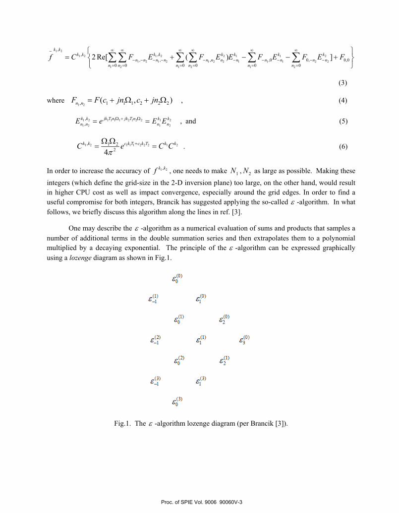
integers (which define the grid-size in the 2-D inversion plane) too large, on the other hand, would result in higher CPU cost as well as impact convergence, especially around the grid edges. In order to find a useful compromise for both integers, Brancik has suggested applying the so-called ε -algorithm. In what follows, we briefly discuss this algorithm along the lines in ref. [3].

One may describe the ε -algorithm as a numerical evaluation of sums and products that samples a number of additional terms in the double summation series and then extrapolates them to a polynomial multiplied by a decaying exponential. The principle of the ε -algorithm can be expressed graphically using a lozenge diagram as shown in Fig.1.

Fig.1. The ε -algorithm lozenge diagram (per Brancik [3]).



All ε terms in the lozenge diagram are matrices with the same order. We manually initialize the

first column ( )1 0sε− = , where s is an integer, and 0 means a zero or null matrix. The second column is

defined as

1 1

1 2

( ,:) ( ,:)( ) ( 1)0 0 , [ ]N s N ss s H

n n IF Eε ε + +−−= + ⊗ , 1,2,....s P= . (7)

In eq. (7), ⊗ is the Kronecker tensor product of matrices. In practice, the extension parameter P is used to justify the result. Thus, the hologram created is assumed to have the order

1 2( 2 ) ( 2 )N P N P+ × + . According to Brancik, the error increases rapidly near far ends of the original 2-D region, thus requiring selection of data from the front (and inner) region of holography. The matrix

1 2,n nF− enters into an 11 2

NM = - point FFT algorithm (along the axis X in the simulation), and the result

is truncated to the order 1 2( 2 )M N P× + . In this one obtains the initial matrix (0)0ε . The matrix next

enters into an 22 2

NM = - point FFT algorithm (along the axis Y in the simulation), and the result is

truncated to the order 1 2M M× . The remaining columns are calculated by a recursion law as follows: ( ) ( 1) ( 1) ( ) 1

1 1 [ ]s s s sr r r rε ε ε ε+ + −+ −= + − , , 1,2,...2r s P= . (8)

The inversion in eq.(3) may now be rewritten in terms of matrices as:

1 2 1 2, ,12 21 11 22 00{2 Re[ ] }k k k kf C G G G G G= + − − +o . (9)

All the terms in eq.(9) are 1 2M M× matrices. The following describe each term in eq.(9):

1 2 2 1,k k k kC C C= ⊗ , (10)

2 100 0,0[ ]M MG F I I= ⊗ , (11)

1 2, 1{ ( )}n nXFFT F Gξ −< >

→ , *1 12{ ( )}

YFFT G Gξ< >

→ , (12)

1 2, 2{ ( )}n nYFFT F Gξ − −< >

→ , *2 21{ ( )}

XFFT G Gξ< >

→ , (13)

2

(:,1)11 1MG I G= ⊗ , and (14)

1

(1,:)22 2MG I G= ⊗ . (15)

The subscript X< > and Y< > are the FFT along axis X and axis Y respectively. The symbol o is the Hadamard product of matrices. {}ζ represents the operator of the ε -algorithm which is applied



ORIGINAL FIGURE (N 1= N2= 512,P =2,c 1 =c2 =0.01)

20

to the result of each FFT operation. 1MI and

2MI are 1 1M × and 21 M× matrices all of whose elements

are equal to 1. (:,1)1G and (1,:)

2G are the Matlab language of 1st column and 1st row of 1G and 2G .

Eq.(9) is useful in computing the inverse of a 2-D Laplace function. The result obtained is impacted by 3 important parameters: the extension coefficient P , the sampling frequency iN , 1,2i = ,

and the coefficients ic , 1,2i = . In the next section, we focus on how the 3 parameter play a role in

determining the correct inverse and finding the optimum parameters. For simplicity, we assume

1 2N N= and 1 2c c= .

3. Simulation results

The motivation for the current work is to simulate numerical 2-D Laplace inversion using eq. (9). In order to make a good comparison, we select 3 test functions whose inverse Laplace expressions are already known.

Case 1

We first consider the 2-D Laplace function

1 21 2 2 2

1 2

( 1)( , ) ( , ) cos( )( 1)( 1)

s sF s s f x y x ys s

−= ↔ = +

+ +, (16)

where f (x,y) is the analytic inverse transform.

Fig.2. The original figure of ( , ) cos( )f x y x y= +



CROSS SECTION OF ORIGINAL FIGURE (N1= N2= 512,P= 2,c1 =c2 =0.01) WHEN X =21

0.8 -

0.6 -

0.4 -

0.2 -

N 0-

-0.2 -

-0.4

-0.6 i

-0.8 -

-1

0 5 10

Y

15 20

N

ALGORITHM FIGURE (N 1= N2= 512,P =2,c 1 =c2 =0.01)

. .- = °-" _. . :: ` c .

0 0

20

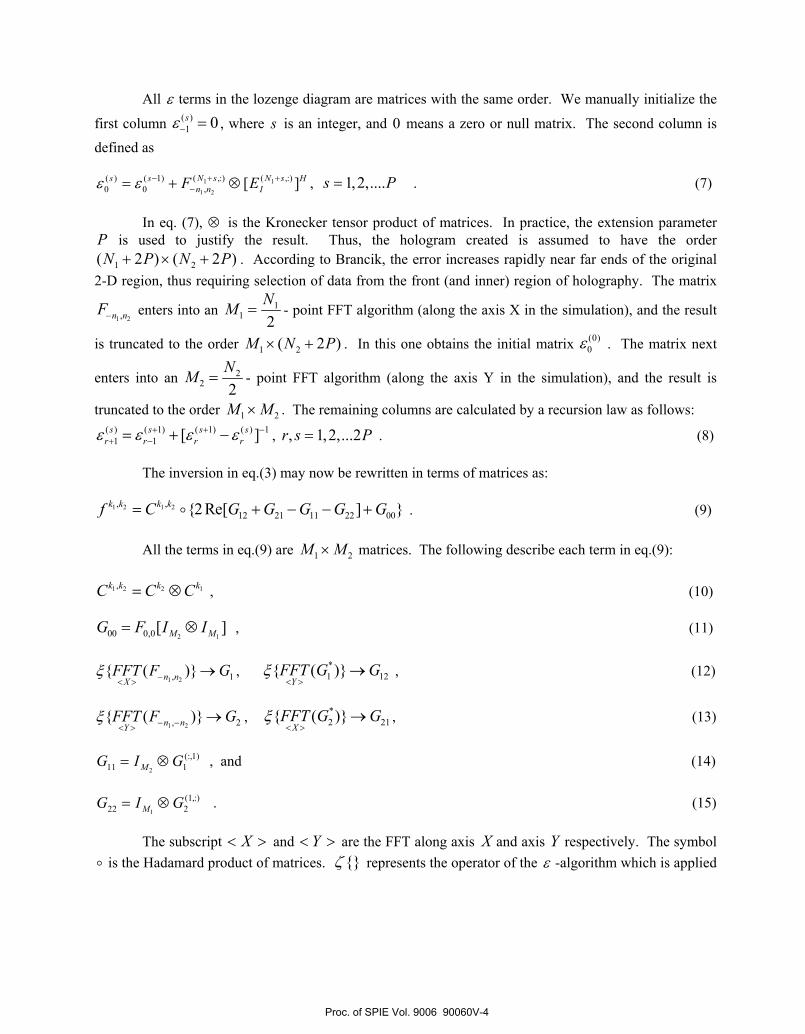
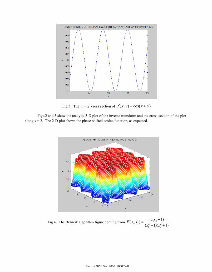
Fig.3. The 2x = cross section of ( , ) cos( )f x y x y= +

Figs.2 and 3 show the analytic 3-D plot of the inverse transform and the cross-section of the plot along x = 2. The 2-D plot shows the phase-shifted cosine function, as expected.

Fig 4. The Brancik algorithm figure coming from 1 21 2 2 2

1 2

( 1)( , )( 1)( 1)

s sF s ss s

−=

+ +



CROSS SECTION OF ALGORITHM FIGURE (N1= N2= 512,P= 2,c1 =c2 =0.01) WHEN X =21

0.8

0.6

0.4

0.2

N

-0.2

-0.4

-0.6

-0.8

-1o 5 10

Y

15 20

CROSS SECTION OF ALGORITHM FIGURE (N1= N2= 512,P= 2,c1= c2 =0.1) WHEN X =21

0.8

0.6

0.4

0.2

N

0

-0.2

-0.4

-0.6

-0.80 5 10

Y

15 20

Fig 5. The 2x = cross section of Fig 4.

Fig 6. The 2x = cross section algorithm figure, but 1 2 0.1c c= = .




0.8 -

0.6 -

0.4

0.2

N

0

-0.2

-0.4

-0.6

-0.80 5 10

Y

15 20


0.8

0.6

0.4

0.2

N

-0.2

-0.4

-0.6

-0.8

-1o 5 10

Y

15 20

Fig 7. The 2x = cross section algorithm figure, but 5P = .

Fig 8. The 2x = cross section algorithm figure, but 1 2 256N N= =




Í011;-7

Y

Fig 9. The 3D figure corresponding to Fig.8.

Figs.4-9 depict a series of plots based on the numerical inversions of the function in eq. (16). Figs.4 and 9 correspond to the 3-D representation with the chosen inversion parameters, whereas Figs.5-8 show 2-D cross sections along x = 2.

Fig.3 is a perfect sine or cosine function with a phase shift. Figs.5-7 show the envelope of the phase-shifted sine function with a relatively steep decay as we change 1 2,c c or P . Figs.3 and 5 are

overall comparable, except for a slight attenuation for larger values of x in Fig.5. Figs.6 and 7 show considerably greater attenuation in the inversion waveform for c1 = c2 = 0.1 and P = 5 respectively. In Fig.8 with the choice of c1 = c2 = 0.01, P = 2, and N1 = N2 = 256, we observe an inversion plot virtually indistinguishable from that of the analytic result in Fig.3. The corresponding 3-D algorithmic plot with these “optimal” parameters, as in Fig.9, appears to be visually lighter; this effect occurs because for a grid number N1 = N2 = 256, the number of generated points within the Matlab program is fewer than with N1 = N2 = 512. Thus, there is a lower density of points with smaller grid number, resulting in the lighter plot visibility. Thus, there is a tradeoff between higher or lower values of N1,N2 in the sense that while higher values of this parameter yields higher density of points, it also leads to increased computational time or CPU cost.



ORIGINAL FIGURE (N1= N2= 512,P= 2,c1 =c2 =0 01)

10X

Y

10

When we compare Fig.5 to Fig.3, we find that the envelope of the sinusoidal plot decays slowly and each extreme point has a left shift which happens in the next two cases as well. In the ‘near’ region, roughly defined in the first half of the plot, the error is less than 5%.

To ascertain the most appropriate opitmal parameter in the Brancik algorithm, we eventually adopted the standard parameters 1 2 1 20.01, 2, 512c c P N N= = = = = , which yield satisfactory results

for a number of inversion simulations. While several test cases were analyzed, we have chosen to discuss only three in this paper.

Case 2

We next examine the 2-D Laplace pair:

21 2 0

1 2 1 2 2

( , ) ( , ) ( ) (2 )( 1)( 1)

sF s s f x y erf x J xy

s s s s s= ↔ =

+ + + . (17)

Fig.10. The original figure of 0( , ) ( ) (2 )f x y erf x J xy= .



CROSS SECTION OF ORIGINAL FIGURE (N1= N2= 512,P= 2,c1 =c2 =0.01) WHEN X =21

0.8

0.6

0.4

N

0.2

-0.2 -

-0.40 10


1111111111il1ú1 11

11 1111181111111111111111111111

11111111111111f Rf R f f RIIl1+p+w i,,

Fig.11. The 2x = cross section of Fig.10.

Fig.12. The Brancik algorithm figure coming from 21 2

1 2 1 2 2

( , )( 1)( 1)

sF s s

s s s s s=

+ + + .



CROSS SECTION OF ALGORITHM FIGURE (N1= N2= 512,P= 2,c1 =c2 =0.01) WHEN X =20.8

0.6 -

0.4 -

0.2

N

0-

-0.2 -

-0.4 -

-0.60 10

Fig 13. The 2x = cross section of Fig.12.

For this problem, we again show the analytic 3-D and 2-D cross section plots in Figs.10 and 11. For optimal parameters as mentioned earlier, we then show the inversion plots obtained from the algorithm. Note the overall similarity between both the 3-D plot and the 2-D section along x = 2 obtained via the algorithm and those from the analytic solution.

The maximum value of the function in Fig.11 is at 0x = . Fig.13 shows the peak to be slightly shifted to the right, implying that a small left shift of the plot in Fig.13 would nearly recover the original plot in Fig.11.

CASE 3

The test function for this case is given below:

1

1 2 01 2

( , ) ( , ) [2 ( 1) ]1

seF s s f x y J x ys s

−

= ↔ = −+

. (18)

Incidentally, this function is the same as the one originally examined by Chatterjee et. al [2] in order to compare the Brancik against the Abate algorithm .



12-10,

86.

N4,2,0,

-2 >4

ORIGINAL FIGURE (N 1= N2= 512,P =2,c 1 =c2 =0.01)

Y0 0

x

ALGORITHM FIGURE (N1= N2= 512,P= 2,c1 =c2 =0.01)

Y0 0

x

Fig.14. The original analytic figure of 0( , ) [2 ( 1) ]f x y J x y= − .

Fig.15. The Brancik algorithm for 1

1 21 2

( , )1

seF s ss s

−

=+

.



CROSS SECTION OF ORIGINAL FIGURE (N1= N2= 512,P= 2,c1 =c2 =0.01) WHEN Y =11r - 1

0.8

0.6

0.4

0.2

0

-0.2

-0.40 0.5 1 1.5 2 2.5 3

x

0

0

0

N

0

CROSS SECTION OF ALGORITHM FIGURE (N1= N2= 512,P= 5,cl =c2 =0.01) WHEN Y =1

-0.2

-0.4

-0.6 i á i i

0.5 1 1.5 2 2.5

x

Fig.16. The 1y = cross section of Fig.14.

Fig.17. The 1y = cross section of Fig.15.



The plots in Figs.14-17 correspond to the two analytic and two algorithmic plots for the chosen test function. Since 1x ≥ is the condition of the original expression, we have to start the comparison beginning at 1x = . The maximum point in Fig.17 is past the range (0,1)x∈ , and slightly to the right. Hence, the ‘left shift’ needed to restore the algorithm to the analytic result still exists. The tendency of each plot to decay and nearly end at 2.0−== fz in the ‘near’ region is evident between Figs.16 and 17; thus, both plots decay to around – 0.2 in the neighborhood of x = 2. Beyond x = 2, the algorithmic plot begins to somewhat diverge from the analytic result. Therefore, for this problem, the “near” region is within the range 1 ≤ x ≤ 2, and for all practical purposes, the inversion is more accurate within this range. We also observe some unexpected oscillation in the neighborhood of about 2x = in Fig.17. Overall, however, within a relatively small (i.e., near) region of the grid coordinates, the algorithm appears to yield reasonably accurate results.

4. Volume holography with 90-degree geometry and Laplace inversion

Banerjee et. al have shown that the two readout beams reconstructed from a 90o volume hologram may be defined via two reduced coupled differential equations [2]:

0 1/e ex jψ κψ∂ ∂ = − , 1 0/e ez jψ κψ∂ ∂ = − (19)

where 2 1/kκ ε ε= is a coupling parameter, 1 22 /k π ε λ= is the propagation constant of the

reconstruction or read wavefront, 0eψ and 1eψ are the zeroth- and first-order readout beams in the phasor

domain. We next present a simple application of the above coupled system to illustrate use of the 2-D Laplace and its inversion in understanding readout from a volume hologram.

Uniform Plane Wave Readout

With the boundary condition for the 0th and 1st orders taken as: 0(0, ) ( )e z Cu zψ = , 1( ,0) 0e xψ = ,

where ( )u z is a unit step in the z direction, and C is a constant. We Laplace transform eq.(19) in 2-D

between ( , )x z and ( , )x zs s to get:

~

0 0 1( , ) ( 0, ) ( , )x e x z e z e x zs s s x s j s sψ ψ κψ− = = − , and (20a)

~

1 1 0( , ) ( , 0) ( , )z e x z e x e x zs s s s z j s sψ ψ κψ− = = − , (20b)

where ~ψ is the Laplace transform of ψ . By solving the above coupled equations, we obtain

~

0 2( , )e x zx z

Cs ss s

ψκ

=+

, ~

1 2( , )( )e x z

z x z

j Cs ss s s

κψκ

−=

+ . (21)



r

CROSS SECTION OF ORIGINAL FIGURE (N1= N2= 512,P =2) WHEN X =2

Z

To obtain the Laplace inversion of the above in 2-D, we next apply the Brancik algorithm, assuming 1 02.5ε ε= , 2 00.4ε ε= , 6

2 10 mλ −= , and 1C = . Analytically, we inverse Laplace transform

eq.(21) first with the respect xs , and then with the respect zs (using a power series expansion), finally

obtain the result:

1 1( , ) (2 )ezx z jC J xzx

ψ κ= . (19)

Generally, the first-order beam is of greater interest, because it represents the diffraction from the hologram, and depicts the reconstructed object wave.

Fig.18. The 2x = cross section of analytic inversion of 1 1( , ) (2 )ezx z jC J xzx

ψ κ= .



T-

1.4

1.2

1

0.8

0.6

0.4

0.2

CROSS SECTION OF ALGORITHM FIGURE (N1= N2= 512,P =2) WHEN X=

,

0.5 1 1.5 2 2.5 3 3.5 4Z

Fig.19. The 2x = cross section arising from numerical inversion of ~

1 2( , )( )e x z

z x z

j Cs ss s s

κψκ

−=

+.

The basic shape and tendencies for both figures are quite similar. We find that both right and left shifts exist at the extreme points in this case. At least so far, we have found that the optimum parameters chosen provide accurate inversion for the uniform plane wave case..

5. Conclusion and further work

In this paper, we were able to determine approximately the optimum inversion parameters needed to apply the Brancik algorithm for 2-D Lapace inversion with some accuracy. Successive runs of the algorithm indicated that the coefficients 1 2,c c impact the values of the extreme (or grid boundary)

points, which leads to envelope decay. Optimal choices were found by selecting

1 2 1 20.01, 512, 2c c N N P= = = = = via a series of comparisons with known analytic test cases. The

results were generally satisfactory, even though there continued to be errors and limitations, especially w.r.t. the grid boundaries, and also the range or size of the inversion map. Laplace inversion is the most direct way to solve the reconstruction problem in holography, but not the only way. Fortunately, the result displayed on Fig.19 provides some confidence that the inversion strategy will likely work for other specific cases involving the object and reference wavefronts in the 90-degree holographic write mode, such as, say, point source illumination or even more general cases. However, as has been seen, there exist left and right shifts in the inverted functions for practically all the cases. Further investigations are needed relative to the properties of the readout beam and its spatial behavior. In order to examine this with greater precision, we intend to use error algorithms to find relative and absolute errors in the inversion on a point by point basis.



References

1. J.W. Goodman, Introduction to Fourier Optics, 3rd edition, McGraw-Hill: New York (2005).

2. M.R. Chatterjee, P.P. Banerjee and G. Nehmetallah, “Analysis of Beam Propagation in 90-Degree Holographic Recording and Readout Using Transfer Functions and Numerical 2-D-Laplace Inversion,” DH Topical Meeting, Vancouver, Canada, PMA6, June 18-20, 2007.

3. L. Brancik “An Improvement of FFT-Based Numerical Inversion of 2D Laplace Transforms by Means of ε -Algorithm” ISCAS-IEEE international Symposium on Circuits and Systems, pp.IV-581-584 (2000).

4. P.P.Banerjee, M.R.Chatterjee, N.Kukhtarev and T.Kukhtareva, "Volume Holographic Recording and Readout for 90-deg Geometry," Opt. Eng. 43, 9, 2053-2060 (Sept. 2004).



Documents

Numerical Inversion and Assessment of 2D Laplace