Embed Size (px)
Citation preview
Waikato Regional Council Technical Report 2012/42
Numerical groundwater flow and transport modelling of the western Lake Taupo catchment www.waikatoregion.govt.nz ISSN 2230-4355 (Print) ISSN 2230-4363 (Online)

Prepared by: Michael Toews, Maksym Gusyev (Institute of Geological and Nuclear Sciences Limited (GNS Science) For: Waikato Regional Council Private Bag 3038 Waikato Mail Centre HAMILTON 3240 January 2012 Document #: 2785154
Doc # 2785154
Peer reviewed by: July 2013 John Hadfield
Approved for release by: Date July 2013 Dominique Noiton
Disclaimer
This technical report has been prepared for the use of Waikato Regional Council as a reference document and as such does not constitute Council’s policy. Council requests that if excerpts or inferences are drawn from this document for further use by individuals or organisations, due care should be taken to ensure that the appropriate context has been preserved, and is accurately reflected and referenced in any subsequent spoken or written communication. While Waikato Regional Council has exercised all reasonable skill and care in controlling the contents of this report, Council accepts no liability in contract, tort or otherwise, for any loss, damage, injury or expense (whether direct, indirect or consequential) arising out of the provision of this information or its use by you or any other party.

Doc # 2785154
Project Number: 632W0505
Numerical Groundwater Flow and Transport Modelling of the Western Lake Taupo Catchment Michael Toews
Maksym Gusyev
GNS Science Consultancy Report 2011/153 January 2012
Doc # 2785154
DISCLAIMER
This report has been prepared by the Institute of Geological and
Nuclear Sciences Limited (GNS Science) exclusively for and under
contract to Waikato Regional Council. Unless otherwise agreed in
writing by GNS Science, GNS Science accepts no responsibility for
any use of, or reliance on any contents of this Report by any person
other than Waikato Regional Council and shall not be liable to any
person other than Waikato Regional Council, on any ground, for any
loss, damage or expense arising from such use or reliance.
The data presented in this Report are available to GNS Science for other use from October 2011
BIBLIOGRAPHIC REFERENCE Toews, M.W.; Gusyev, M.A. 2011. Numerical Groundwater Flow and Transport Modelling of the Western Lake Taupo Catchment, GNS Science Consultancy Report 2011/153. 31p.
Confidential 2011
GNS Science Consultancy Report 2011/153 i
CONTENTS
EXECUTIVE SUMMARY ........................................................................................................ II
1.0 INTRODUCTION ........................................................................................................ 1
2.0 MODEL DESIGN ........................................................................................................ 1
2.1 Conceptual Model .......................................................................................... 1 2.2 Model Grid ..................................................................................................... 2 2.3 Hydrogeological Properties ............................................................................ 2 2.4 Boundary Conditions ...................................................................................... 2
2.4.1 No flow ............................................................................................... 3 2.4.2 Groundwater recharge ........................................................................ 3 2.4.3 Surface water features ........................................................................ 3 2.4.4 Nitrate loading .................................................................................... 3
2.5 Calibration Targets ......................................................................................... 4 2.5.1 Stream flow ......................................................................................... 4 2.5.2 Groundwater levels ............................................................................. 4 2.5.3 Mean residence time ........................................................................... 4
3.0 MODEL CALIBRATION ............................................................................................. 5
3.1 Model Run Setting .......................................................................................... 5 3.2 Calibration to Stream Flow ............................................................................. 5 3.3 Calibration to Groundwater Levels ................................................................. 6 3.4 Calibration to Mean Residence Time .............................................................. 6 3.5 Sensitivity and Uncertainty ............................................................................. 6
4.0 MODEL PREDICTIONS ............................................................................................. 7
4.1 Groundwater Flow Results ............................................................................. 7 4.2 Nitrate Transport Results................................................................................ 7
5.0 SUMMARY AND RECOMMENDATIONS ................................................................... 7
6.0 ACKNOWLEDGEMENTS........................................................................................... 9
7.0 REFERENCES ........................................................................................................... 9
FIGURES
Figure 1. The domain of the western Lake Taupo catchment numerical model. ............................................. 12 Figure 2. Cross sections at row 344 of the uniform 80 m wide by 20 m thick grid with 'A' unadjusted
DTM and 'B' adjusted DTM.. ............................................................................................................ 13 Figure 3. Plan view of model, showing the top layer of the hydrostratigraphy. ................................................ 14 Figure 4. Cross sections through model showing hydrostratigraphy of materials along rows 129, 186,
299, 330 and 429. ............................................................................................................................ 15 Figure 5. Boundary conditions for groundwater flow model. ........................................................................... 16 Figure 6. Nitrate loading used as a constant concentration boundary condition on the topmost
saturated cells or water table (Hadfield 2011).. ................................................................................ 17 Figure 7. Zones used for ZONEBUDGET (ZBUD) to calibrate stream gauges.. ............................................. 18 Figure 8. Groundwater observation wells in the model domain used for groundwater flow model
calibration (Gusyev et al. 2011). ...................................................................................................... 19 Figure 9. Simulated vs. observed stream/river flows, units are m³/s. .............................................................. 20 Figure 10. Calibration plot of modelled vs. observed hydraulic head in the steady-state groundwater
flow model. ....................................................................................................................................... 21 Figure 11. Contour-fill map of groundwater table from steady-state flow simulation.. ....................................... 22 Figure 12. Cross sections showing groundwater flow and nitrate simulation results in mg/L. ........................... 23
TABLES Table 1. Data summary of 27 surface water sub-catchments in the western Lake Taupo catchment
area (Gusyev et al. 2011). ................................................................................................................ 25 Table 2. Hydrogeologic properties of materials used for the model development model calibration. ............. 26 Table 3. Steady-state groundwater flow budget. ............................................................................................ 26
Doc # 2785154
EXECUTIVE SUMMARY
The goal of this study was to develop a steady-state groundwater flow and transient
contaminant transport model to aid with nitrate management in the western Lake Taupo
catchment. The model was developed in Visual MODFLOW Pro (VMOD) using available field
data and the proposed model design from Gusyev et al. (2011). The model development
consisted of two steps: model design and model predictions. The model design included
implementation of model grid, boundary conditions, hydrogeology, calibration targets and
model calibration. The model predictions included modelled groundwater elevations, water
budgets and tentative nitrate concentrations.
The MODFLOW grid covered the modelling area of 1072 km² with 500 rows and 335
columns and had a uniform cell size of 80 m by 80 m. The model depth of 320 m
incorporated 16 layers with a constant layer thickness of 20 m. The top of the model grid was
obtained from modified digital terrain surface and Lake Taupo bathymetry data.
The hydrogeology of the modelling area is comprised of aggregated units of Oruanui,
Whakamaru, Pakaumanu and Greywacke (Gusyev et al. 2011). Each grid cell was
associated with one hydrogeologic unit and assigned hydraulic conductivity and porosity
properties of the unit.
The following boundary conditions (BCs) were applied to the groundwater flow and nitrate
transport model: a constant head BC was used to represent water elevations in Lake Taupo;
a Cauchy head-dependant BC was used to represent rivers/streams; a flux BC was used to
represent groundwater recharge; and a constant concentration specified flux BC was used to
represent nitrate loading. These BCs were assigned to layer 1 except the nitrate loading that
was implemented to the top-most saturated layer (Gusyev et al. 2011).
The steady-state groundwater flow model was simulated with MODFLOW-2000 and
calibrated for stream flows and hydraulic heads by adjusting groundwater recharge, river bed
conductance and hydraulic conductivities. The groundwater travel times were simulated with
MODPATH and calibrated to Mean Residence Times (MRTs), obtained from groundwater
age tracers for the western Lake Taupo area, by adjusting aquifer porosity.
Nitrate transport was simulated as a non-reactive species with MT3DMS 5.2. The transport
simulation was conducted for 100 years, with concentrations output every 10 years.
Calibration of the nitrate transport model was not undertaken as it was beyond the scope of
this study. Modelled nitrate concentrations extend down through Oruanui and Whakamaru
units after 80 years.
The results from the groundwater flow model indicate groundwater elevations ranging from
357 m at the Lake Taupo lakeshore to over 1000 m in the northern part of the model domain.
Modelled groundwater elevations are sensitive to hydraulic conductivities of Oruanui and
Whakamaru units. Decreasing hydraulic conductivity of the Oruanui unit resulted in higher
groundwater mounding along Karangahape Road (centre of domain), and consequently
fewer dry cells in the flow model. The modelled MRTs for Waihaha River, Wanganui Stream,
Whareroa Stream, and Kuratau River sub-catchments, using cumulative frequency
distribution curves, were 36 years, 30 years, 51 years and 35 years, respectively. Preliminary
Confidential 2011
GNS Science Report 2011/153 iii
results of the transport model indicate that nitrate plumes extended through the Oruanui and
parts of Whakamaru units and reached Lake Taupo after 80 years simulation time.
The following five items are recommended for the next phase of the nitrate transport model
development:
1) Areas of high modelled nitrate concentration need to be refined. Such plumes may
introduce errors in nitrate transport model calibration unless model refinement is
undertaken.
2) Calibration targets for nitrate concentration need to be implemented in the transport
model.
3) Groundwater tracer concentrations such as tritium should be implemented as primary
calibration targets for the transport model.
4) Sensitivity analysis and uncertainty analysis should be conducted on the calibrated
transport model.
5) Modelling of management scenarios for the western Lake Taupo catchment should be
undertaken using the calibrated groundwater flow and transport model.

Confidential 2011
GNS Science Report 2011/153 1
1.0 INTRODUCTION
The goal of this study was to develop a steady-state groundwater flow and transient
contaminant transport model to aid with nitrate management in the western Lake Taupo
catchment. This study is a continuation of the study by Gusyev et al. (2011) and provides a
detailed description of the constructed model for the western Lake Taupo catchment (Figure
1). Gusyev et al. (2011) summarized available field data and proposed a suitable model
design for the western Lake Taupo catchment using Visual MODFLOW Pro (VMOD)
(Schlumberger Water Services 2010).
An effective modelling exercise consists of four general steps. In the first preliminary step,
the purpose of the modelling is defined (Bear et al. 1992). A conceptual model is constructed
for the area of interest and the modelling code selected. In the second step, the model is
designed. In the third step, the model is calibrated to field observations and is tested with a
sensitivity analysis, which determines the variability in modelling results due to the change in
calibrated parameters. In the final step, the parameter uncertainty analysis determines the
bounds of the uncertainty interval for model outcomes associated with different sets of
parameters (Hill and Tiedeman 2007).
This report follows these steps and is divided in three sections: model design, model
calibration and model predictions. The model design consisted of grid design, selection of
boundary conditions, implementation of hydrogeology, and implementation of calibration
targets. Each step of the model design required simplifying assumptions to represent the
complexities of the natural flow system that are addressed by Gusyev et al. (2011). Model
calibration consisted of calibration, sensitivity and uncertainty, and determined the effect of
parameters on the modelling results. The steady-state groundwater flow model was
calibrated to median values of stream flows and groundwater levels and to Mean Residence
Times (MRTs) obtained from groundwater age tracer data. The calibration of transient nitrate
transport to measured concentrations was beyond the scope of this study and not
undertaken. The sensitivity analysis was carried out for hydraulic conductivity values in the
groundwater flow model. The uncertainty analysis was not implemented at this stage of the
project and will be conducted for the groundwater flow and transport model using automated
Parameter Estimation software (PEST). The calibrated groundwater flow model was used to
simulate contaminant transport and to predict nitrate concentrations discharging into Lake
Taupo. Model predictions consisted of modelled groundwater elevations, water budgets and
tentative nitrate concentrations. Modelling results of nitrate transport are presented to provide
understanding of nitrate movement in the groundwater system. The effects of groundwater
flow model assumptions on the modelling results for contaminant transport are also
discussed.
2.0 MODEL DESIGN
2.1 Conceptual Model
A conceptual model for the western Lake Taupo catchment was presented by Gusyev et al.
(2011). In summary, the aquifer system is assumed to be bounded by the Lake Taupo
surface catchment boundary in the west and by the lake bed in the east (Figure 1). The north
and south sides of the model are also surface catchment boundaries (i.e. the conceptual
Doc # 2785154
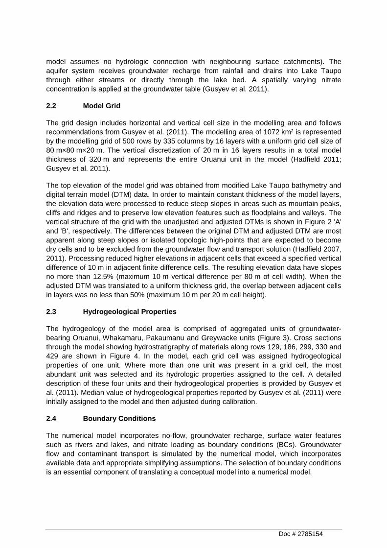
model assumes no hydrologic connection with neighbouring surface catchments). The
aquifer system receives groundwater recharge from rainfall and drains into Lake Taupo
through either streams or directly through the lake bed. A spatially varying nitrate
concentration is applied at the groundwater table (Gusyev et al. 2011).
2.2 Model Grid
The grid design includes horizontal and vertical cell size in the modelling area and follows
recommendations from Gusyev et al. (2011). The modelling area of 1072 km² is represented
by the modelling grid of 500 rows by 335 columns by 16 layers with a uniform grid cell size of
80 m×80 m×20 m. The vertical discretization of 20 m in 16 layers results in a total model
thickness of 320 m and represents the entire Oruanui unit in the model (Hadfield 2011;
Gusyev et al. 2011).
The top elevation of the model grid was obtained from modified Lake Taupo bathymetry and
digital terrain model (DTM) data. In order to maintain constant thickness of the model layers,
the elevation data were processed to reduce steep slopes in areas such as mountain peaks,
cliffs and ridges and to preserve low elevation features such as floodplains and valleys. The
vertical structure of the grid with the unadjusted and adjusted DTMs is shown in Figure 2 'A'
and 'B', respectively. The differences between the original DTM and adjusted DTM are most
apparent along steep slopes or isolated topologic high-points that are expected to become
dry cells and to be excluded from the groundwater flow and transport solution (Hadfield 2007,
2011). Processing reduced higher elevations in adjacent cells that exceed a specified vertical
difference of 10 m in adjacent finite difference cells. The resulting elevation data have slopes
no more than 12.5% (maximum 10 m vertical difference per 80 m of cell width). When the
adjusted DTM was translated to a uniform thickness grid, the overlap between adjacent cells
in layers was no less than 50% (maximum 10 m per 20 m cell height).
2.3 Hydrogeological Properties
The hydrogeology of the model area is comprised of aggregated units of groundwater-
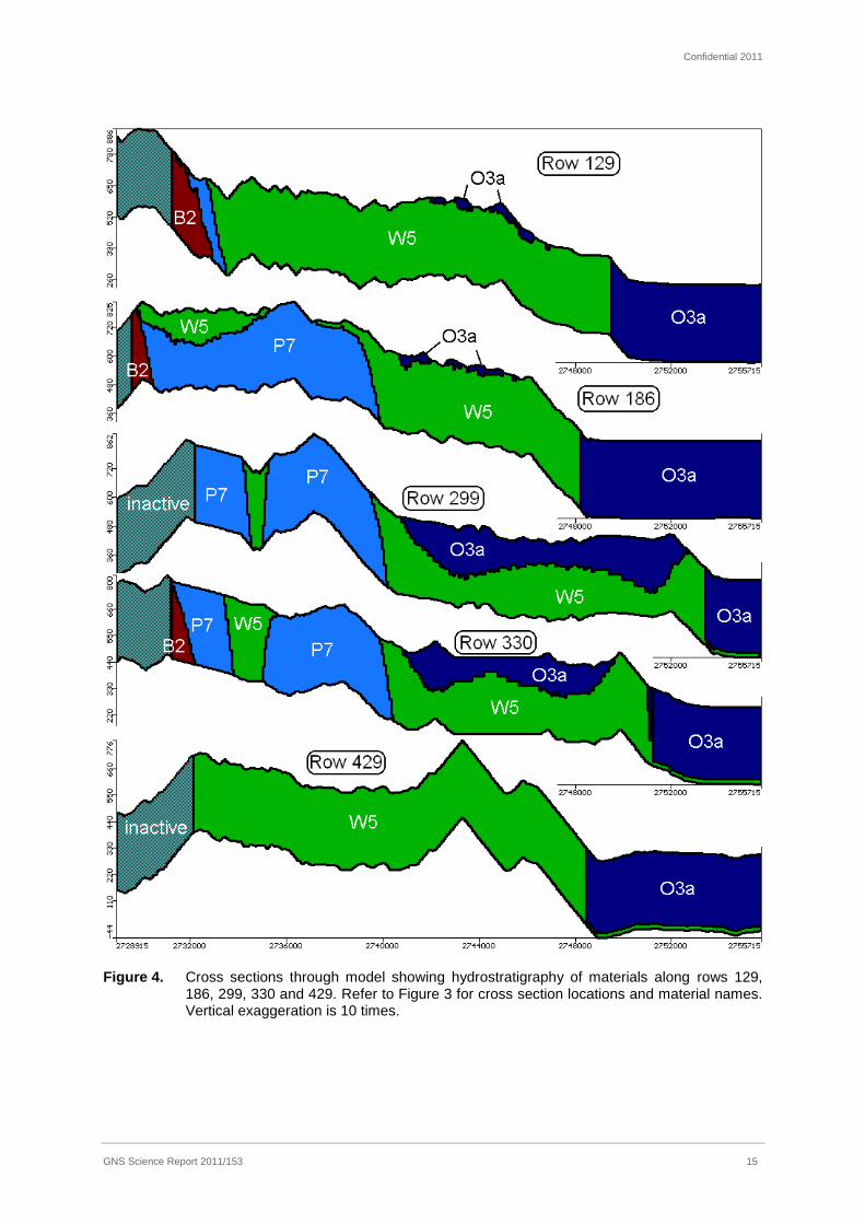
bearing Oruanui, Whakamaru, Pakaumanu and Greywacke units (Figure 3). Cross sections
through the model showing hydrostratigraphy of materials along rows 129, 186, 299, 330 and
429 are shown in Figure 4. In the model, each grid cell was assigned hydrogeological
properties of one unit. Where more than one unit was present in a grid cell, the most
abundant unit was selected and its hydrologic properties assigned to the cell. A detailed
description of these four units and their hydrogeological properties is provided by Gusyev et
al. (2011). Median value of hydrogeological properties reported by Gusyev et al. (2011) were
initially assigned to the model and then adjusted during calibration.
2.4 Boundary Conditions
The numerical model incorporates no-flow, groundwater recharge, surface water features
such as rivers and lakes, and nitrate loading as boundary conditions (BCs). Groundwater
flow and contaminant transport is simulated by the numerical model, which incorporates
available data and appropriate simplifying assumptions. The selection of boundary conditions
is an essential component of translating a conceptual model into a numerical model.
Confidential 2011
GNS Science Report 2011/153 3
2.4.1 No flow
Grid cells outside of the modelled groundwater catchment are assigned no flow boundary
condition (inactive cells in MODFLOW), and therefore are not included in the groundwater
flow and contaminant transport solution (Figure 3 and 4). In order to improve stability of the
finite difference solution, the border of the active/inactive interface was analysed to ensure
that all active cells had at least two active adjacent cells. As the result, 16 border active cells
were identified in each layer and changed to inactive cells.
2.4.2 Groundwater recharge
The difference of average annual rainfall and actual evaporation data between 1960 and
2006 was used as groundwater recharge in the model (Gusyev et al. 2011). The
groundwater recharge values were gridded to 80 m cell model resolution and reclassified into
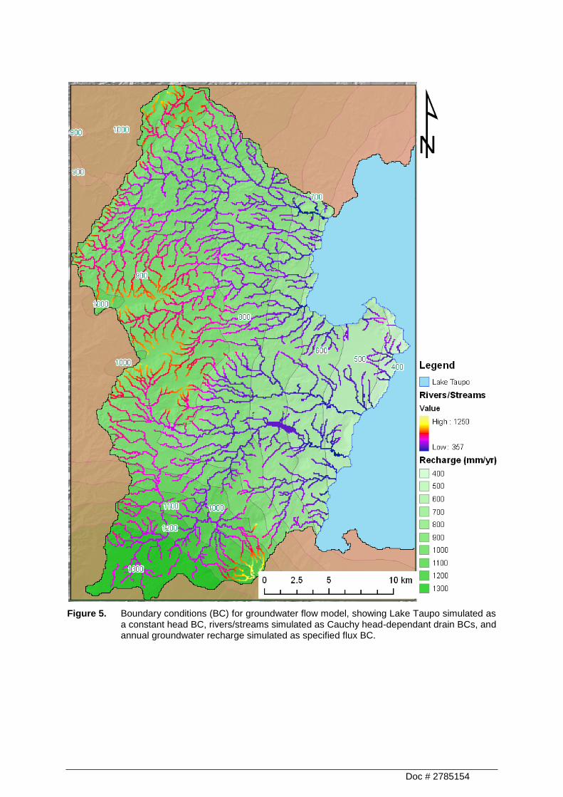
10 zones (Figure 5). Each zone has a discrete recharge value from 400 to 1300 mm/year
with 100 mm/year increments. These values were assigned to the topmost saturated model
layer using the MODFLOW recharge option #3 (McDonald and Harbaugh 1988; Harbaugh et
al. 2000).
2.4.3 Surface water features
The Lake Taupo water level is incorporated in the model as a constant head boundary
condition and was set to an elevation of 357 m. The constant head boundary cells were
implemented at the lake bed in layer 1 of the model.
Rivers and small streams are incorporated in layer 1 of the model as a Cauchy boundary
condition with the use of drain cells. In MODFLOW, a drain cell is a head-dependant Cauchy
boundary that removes water from the groundwater system only when the modelled
hydraulic head is greater than the drain bottom elevation. Water elevations in the drain cells
were obtained from the top elevation of layer 1 and the assigned drain bottom elevation was
1 m below the top elevation of layer 1. A uniform conductance of 80 m²/day was assigned to
all drain cells in the model. The locations of the drain cells were obtained from the 1:50 000
topographic dataset based on vector data of the streams.
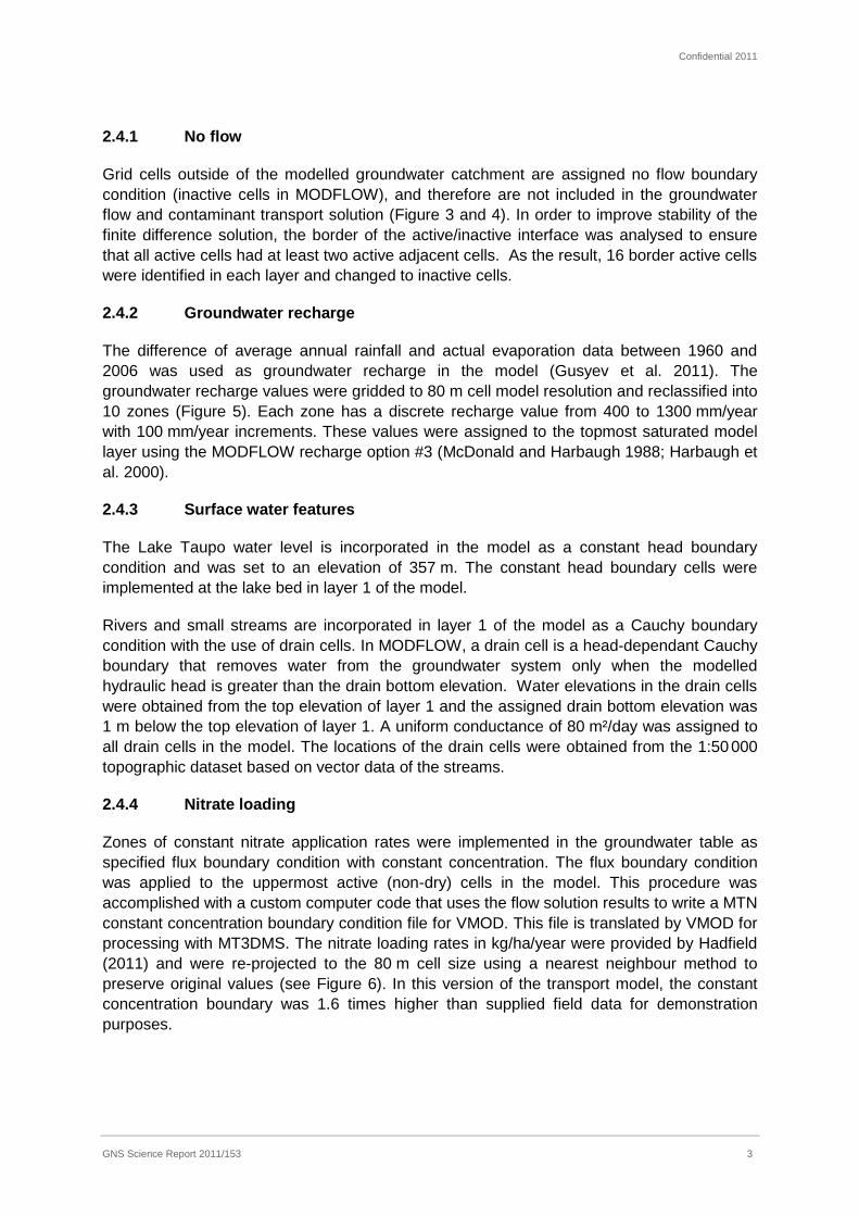
2.4.4 Nitrate loading
Zones of constant nitrate application rates were implemented in the groundwater table as
specified flux boundary condition with constant concentration. The flux boundary condition
was applied to the uppermost active (non-dry) cells in the model. This procedure was
accomplished with a custom computer code that uses the flow solution results to write a MTN
constant concentration boundary condition file for VMOD. This file is translated by VMOD for
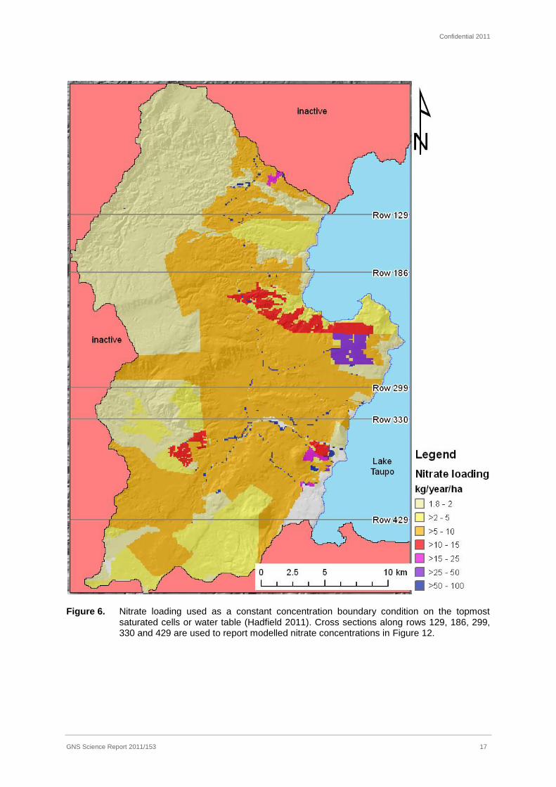
processing with MT3DMS. The nitrate loading rates in kg/ha/year were provided by Hadfield
(2011) and were re-projected to the 80 m cell size using a nearest neighbour method to
preserve original values (see Figure 6). In this version of the transport model, the constant
concentration boundary was 1.6 times higher than supplied field data for demonstration
purposes.
Doc # 2785154
2.5 Calibration Targets
Generally, data sets of stream flow, groundwater levels and chemical concentrations
obtained from field measurements are used as model calibration targets. Recently, mean
residence time (MRT) estimated from groundwater age tracers has also been used for the
calibration of aquifer porosity in groundwater flow models (McGuire & McDonnell 2006). The
following calibration targets identified by Gusyev et al. (2011) were used in this study: 30
stream gauging stations with non-zero flow measurements; 24 boreholes with adequate
groundwater level observations; and 5 surface water sub-catchments with MRT values. In
this study, chemical concentrations are not implemented as calibration targets for the
transport model.
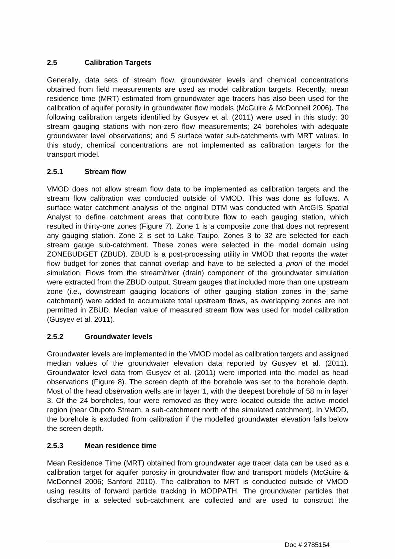
2.5.1 Stream flow
VMOD does not allow stream flow data to be implemented as calibration targets and the
stream flow calibration was conducted outside of VMOD. This was done as follows. A
surface water catchment analysis of the original DTM was conducted with ArcGIS Spatial
Analyst to define catchment areas that contribute flow to each gauging station, which
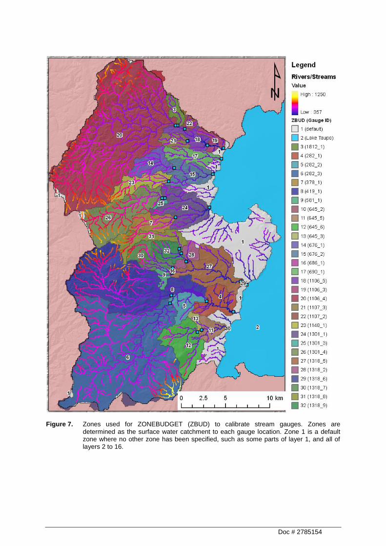
resulted in thirty-one zones (Figure 7). Zone 1 is a composite zone that does not represent
any gauging station. Zone 2 is set to Lake Taupo. Zones 3 to 32 are selected for each
stream gauge sub-catchment. These zones were selected in the model domain using
ZONEBUDGET (ZBUD). ZBUD is a post-processing utility in VMOD that reports the water
flow budget for zones that cannot overlap and have to be selected a priori of the model
simulation. Flows from the stream/river (drain) component of the groundwater simulation
were extracted from the ZBUD output. Stream gauges that included more than one upstream
zone (i.e., downstream gauging locations of other gauging station zones in the same
catchment) were added to accumulate total upstream flows, as overlapping zones are not
permitted in ZBUD. Median value of measured stream flow was used for model calibration
(Gusyev et al. 2011).
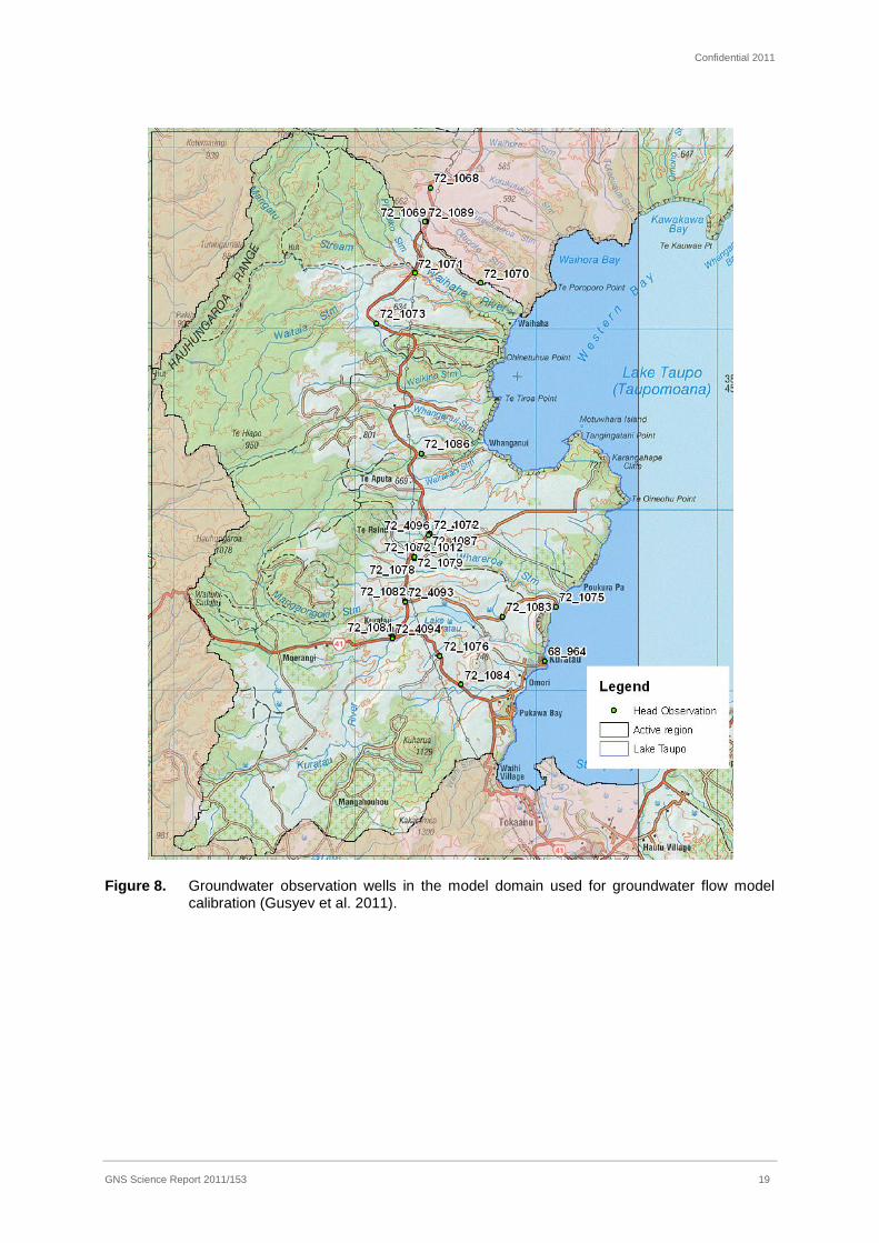
2.5.2 Groundwater levels
Groundwater levels are implemented in the VMOD model as calibration targets and assigned
median values of the groundwater elevation data reported by Gusyev et al. (2011).
Groundwater level data from Gusyev et al. (2011) were imported into the model as head
observations (Figure 8). The screen depth of the borehole was set to the borehole depth.
Most of the head observation wells are in layer 1, with the deepest borehole of 58 m in layer
3. Of the 24 boreholes, four were removed as they were located outside the active model
region (near Otupoto Stream, a sub-catchment north of the simulated catchment). In VMOD,
the borehole is excluded from calibration if the modelled groundwater elevation falls below
the screen depth.
2.5.3 Mean residence time
Mean Residence Time (MRT) obtained from groundwater age tracer data can be used as a
calibration target for aquifer porosity in groundwater flow and transport models (McGuire &
McDonnell 2006; Sanford 2010). The calibration to MRT is conducted outside of VMOD
using results of forward particle tracking in MODPATH. The groundwater particles that
discharge in a selected sub-catchment are collected and are used to construct the
Confidential 2011
GNS Science Report 2011/153 5
cumulative frequency distribution curve at the sub-catchment outlet. The cumulative
frequency distribution curve is a mixture of groundwater ages, reflecting the different transit
times along all of the flow paths that converge at the sampling point such as outflow from a
surface water sub-catchment (McDonnell et al. 2010).
3.0 MODEL CALIBRATION
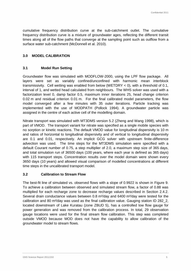
3.1 Model Run Setting
Groundwater flow was simulated with MODFLOW-2000, using the LPF flow package. All
layers were set as variably confined/unconfined with harmonic mean interblock
transmissivity. Cell wetting was enabled from below (WETDRY < 0), with a threshold of 0.1,
interval of 1, and wetted head calculated from neighbours. The WHS solver was used with a
factorization level 0, damp factor 0.5, maximum inner iterations 25, head change criterion
0.02 m and residual criterion 0.01 m. For the final calibrated model parameters, the flow
model converged after a few minutes with 35 outer iterations. Particle tracking was
implemented with the use of MODPATH (Pollock 1994). A groundwater particle was
assigned in the centre of each active cell of the modelling domain.
Nitrate transport was simulated with MT3DMS version 5.2 (Zheng and Wang 1998), which is
part of VMOD. The transport variant for nitrate was specified as a single mobile species with
no sorption or kinetic reactions. The default VMOD value for longitudinal dispersivity is 10 m
and ratios of horizontal to longitudinal dispersivity and of vertical to longitudinal dispersivity
are 0.1 and 0.01, respectively. An implicit GCG solver with upstream finite-difference
advection was used. The time steps for the MT3DMS simulation were specified with a
default Courant number of 0.75, a step multiplier of 2.0, a maximum step size of 365 days,
and total simulation run of 36500 days (100 years, where each year is defined as 365 days)
with 115 transport steps. Concentration results over the model domain were shown every
3650 days (10 years) and allowed visual comparison of modelled concentrations at different
time steps in the uncalibrated transport model.
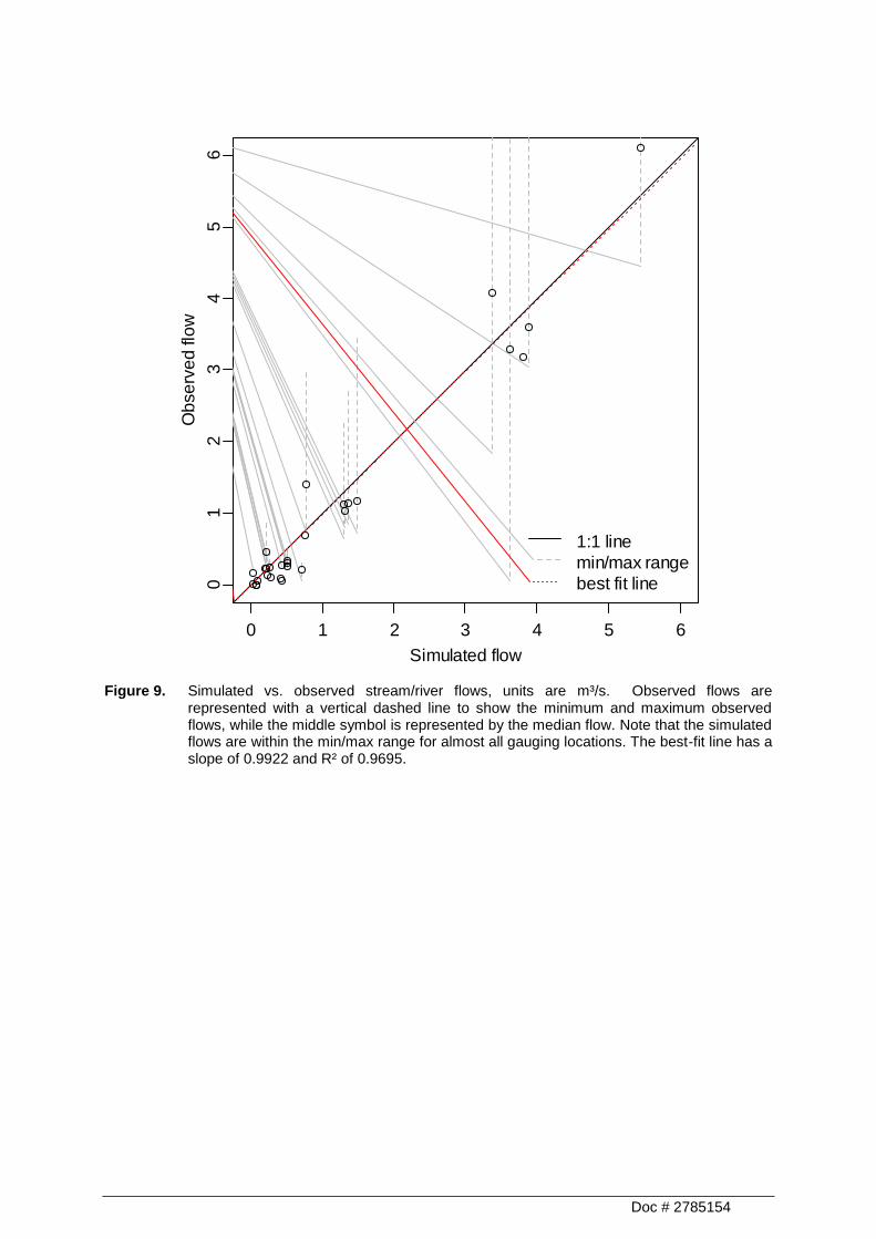
3.2 Calibration to Stream Flow
The best-fit line of simulated vs. observed flows with a slope of 0.9922 is shown in Figure 9.
To achieve a calibration between observed and simulated stream flow, a factor of 0.88 was
multiplied for each recharge zone to decrease recharge values described in Section 2.4.2.
Several drain conductance values between 0.8 m²/day and 6400 m²/day were tested for the
calibration and 80 m²/day was used as the final calibration value. Gauging station ID 282_2,
located downstream of Lake Kuratau (zone ZBUD 5), has a controlled low flow gauge for
power generation and was removed from the calibration process. In total, 29 observation
gauge locations were used for the final stream flow calibration. This step was completed
outside VMOD because MOD does not have the capability to allow calibration of the
groundwater model to stream flows.
Doc # 2785154
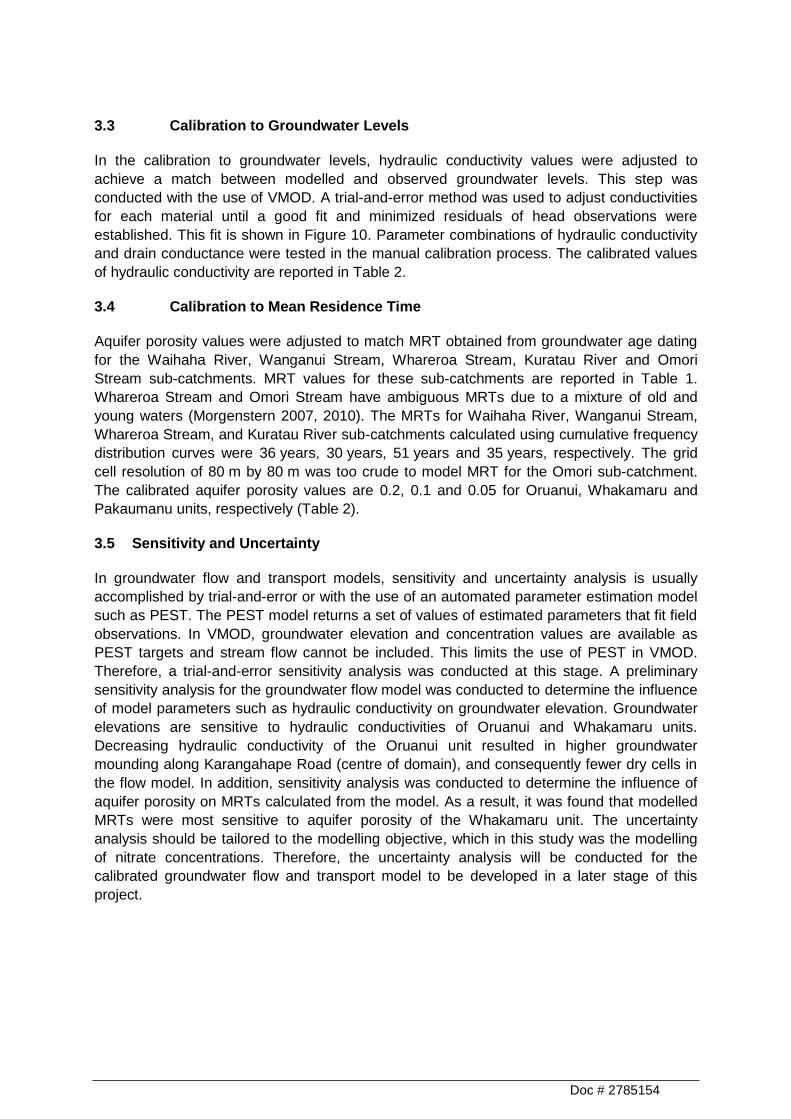
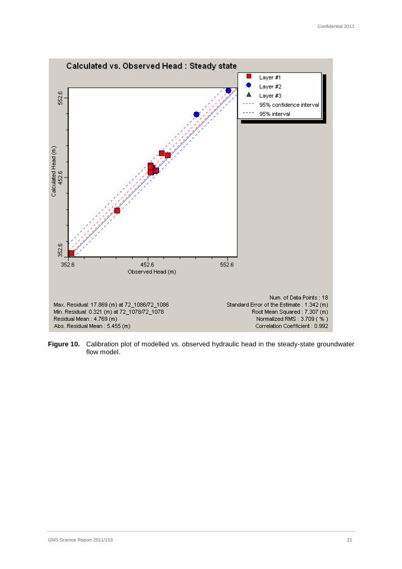
3.3 Calibration to Groundwater Levels
In the calibration to groundwater levels, hydraulic conductivity values were adjusted to
achieve a match between modelled and observed groundwater levels. This step was
conducted with the use of VMOD. A trial-and-error method was used to adjust conductivities
for each material until a good fit and minimized residuals of head observations were
established. This fit is shown in Figure 10. Parameter combinations of hydraulic conductivity
and drain conductance were tested in the manual calibration process. The calibrated values
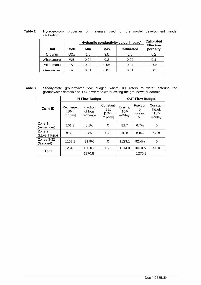
of hydraulic conductivity are reported in Table 2.
3.4 Calibration to Mean Residence Time
Aquifer porosity values were adjusted to match MRT obtained from groundwater age dating
for the Waihaha River, Wanganui Stream, Whareroa Stream, Kuratau River and Omori
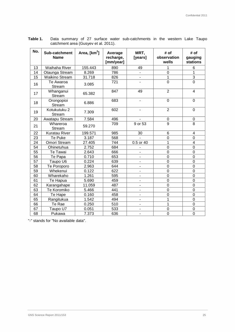
Stream sub-catchments. MRT values for these sub-catchments are reported in Table 1.
Whareroa Stream and Omori Stream have ambiguous MRTs due to a mixture of old and
young waters (Morgenstern 2007, 2010). The MRTs for Waihaha River, Wanganui Stream,
Whareroa Stream, and Kuratau River sub-catchments calculated using cumulative frequency
distribution curves were 36 years, 30 years, 51 years and 35 years, respectively. The grid
cell resolution of 80 m by 80 m was too crude to model MRT for the Omori sub-catchment.
The calibrated aquifer porosity values are 0.2, 0.1 and 0.05 for Oruanui, Whakamaru and
Pakaumanu units, respectively (Table 2).
3.5 Sensitivity and Uncertainty
In groundwater flow and transport models, sensitivity and uncertainty analysis is usually
accomplished by trial-and-error or with the use of an automated parameter estimation model
such as PEST. The PEST model returns a set of values of estimated parameters that fit field
observations. In VMOD, groundwater elevation and concentration values are available as
PEST targets and stream flow cannot be included. This limits the use of PEST in VMOD.
Therefore, a trial-and-error sensitivity analysis was conducted at this stage. A preliminary
sensitivity analysis for the groundwater flow model was conducted to determine the influence
of model parameters such as hydraulic conductivity on groundwater elevation. Groundwater
elevations are sensitive to hydraulic conductivities of Oruanui and Whakamaru units.
Decreasing hydraulic conductivity of the Oruanui unit resulted in higher groundwater
mounding along Karangahape Road (centre of domain), and consequently fewer dry cells in
the flow model. In addition, sensitivity analysis was conducted to determine the influence of
aquifer porosity on MRTs calculated from the model. As a result, it was found that modelled
MRTs were most sensitive to aquifer porosity of the Whakamaru unit. The uncertainty
analysis should be tailored to the modelling objective, which in this study was the modelling
of nitrate concentrations. Therefore, the uncertainty analysis will be conducted for the
calibrated groundwater flow and transport model to be developed in a later stage of this
project.
Confidential 2011
GNS Science Report 2011/153 7
4.0 MODEL PREDICTIONS
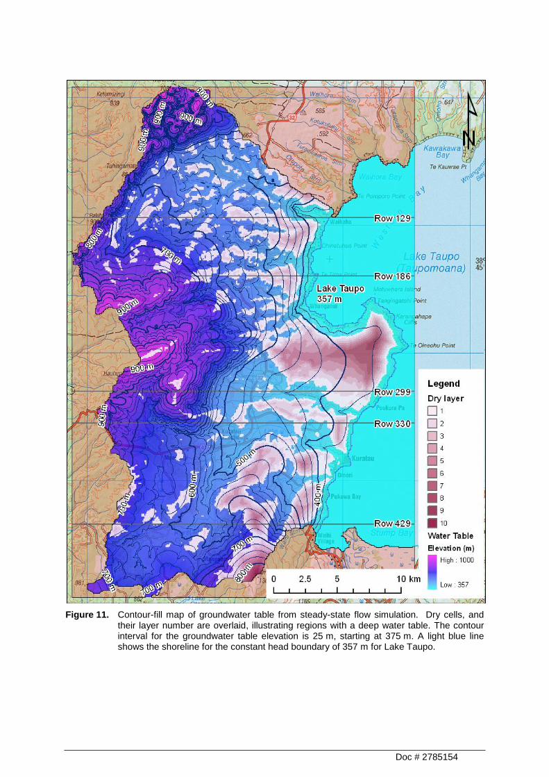
4.1 Groundwater Flow Results
Modelled groundwater elevations and the water budget obtained from the calibrated
groundwater flow model are shown in Figure 11 and Table 3, respectively. In Figure 11, the
modelled groundwater elevations vary from 357 m at the Lake Taupo lakeshore (shown by a
light blue line) to over 1000 m in the northern part of the model domain. Dry cells occur along
ridges and at topographic high points, and are often found in the Oruanui unit. Dry cells
extend from layer 1 down to layer 10, where the water table is approximately 200 m below
the top of the model. Cells with either greywacke or Pakaumanu units are normally always
saturated as the hydraulic conductivities of these units are relatively low. In Table 3, the
modelled In and Out water balance indicate good model convergence, which was a
requirement of the study (Hadfield 2011).
4.2 Nitrate Transport Results
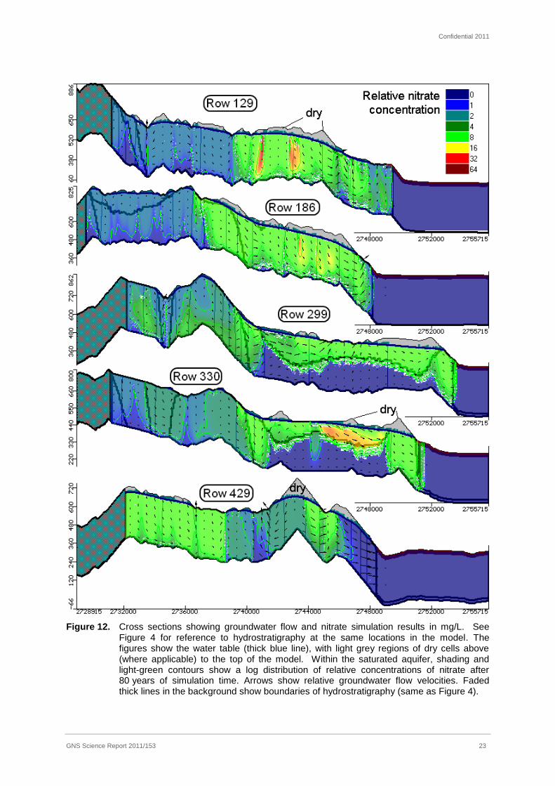
Modelling results for nitrate transport simulation at 80 years simulation time are shown in
Figure 12 for cross sections along rows 129, 186, 299, 330 and 429. In Figure 12, relative
concentrations of simulated nitrate are colour-coded and contoured with light green lines
from 0 (background) to 64 mg/L using a log2 scale. Nitrate concentrations are relative in
Figure 12 as the specified concentration from nitrate loading (Figure 6) is not scaled from the
original units of kg/year/ha to more appropriate units of concentrations (i.e., mg/L). The
groundwater table is shown as a thick blue line and the relative groundwater flow velocities
are represented by arrows. The magnitude of modelled groundwater velocity up to a
maximum velocity of 0.75 m/day is indicated by the size of arrows. Arrows point upwards out
of the top surface where groundwater is discharging. The dry cells that occur in the top layers
of the flow model are shown by light grey regions. The hydrostratigraphy of cross sections is
shown by faded thick lines in the background and is described earlier in this report (Figure 4).
Modelled plumes of nitrate extended through the Oruanui and parts of Whakamaru units at
80 years simulation time. In the cross sections at row 299 and 330 of Figure 12, the extent of
the nitrate plume follows the hydrostratigraphic boundary between Oruanui and Whakamaru
units. This phenomenon is due to the different hydraulic conductivities used for the two units,
where preferential flow is in the more permeable Oruanui unit, and some flow is refracted at
a shallower angle in the less permeable Whakamaru unit (Freeze & Cherry 2003).
Nitrate concentrations in modelled plumes are sensitive to nitrate loading data, as shown in
row 129 on the map in Figure 6 and in profile in Figure 12. In this profile, a few cells along
parts of Western Bay Road (SH32) have approximately 60 kg/year/ha. These few cells of
high concentration are shown in the cross section as elongated subsurface plumes of nitrate.
5.0 SUMMARY AND RECOMMENDATIONS
A groundwater flow and nitrate transport model has been developed for the western Lake
Taupo catchment using cutting-edge groundwater modelling techniques. The resolution of
the model grid was selected to provide accurate nitrate transport simulations and to include
small surface water features such as streams (Gusyev et al. 2011). Aquifer hydrogeology
Doc # 2785154
was incorporated in the model based on representation of the geologic units. The nitrate flux
boundary condition was applied to the uppermost active (non-dry) cells in the model. The
groundwater flow model was calibrated to median values of groundwater elevation and
stream flow data (Hadfield 2011; Gusyev et al. 2011). In the calibration to stream flow,
groundwater recharge and drain conductance values were adjusted to match median values
of observed stream flows at gauging stations outside of VMOD. In addition, particle tracking
with MODPATH was implemented in the model and used to calibrate aquifer porosity to MRT
obtained from groundwater age tracers (Gusyev et al. 2011). Calibration of the nitrate
transport model was not undertaken as it was beyond the scope of this study.
The results of this groundwater flow model indicate groundwater elevations ranging from
357 m at the Lake Taupo lakeshore to over 1000 m in the northern part of the model domain.
Modelled groundwater elevations are sensitive to hydraulic conductivities of Oruanui and
Whakamaru units. Decreasing hydraulic conductivity of the Oruanui unit resulted in higher
groundwater mounding along Karangahape Road (centre of domain), and consequently
fewer dry cells in the flow model. The modelled MRTs for Waihaha River, Whareroa Stream,
and Kuratau River sub-catchments, using cumulative frequency distribution curves, were
36 years, 51 years and 35 years, respectively. Preliminary results of the transport model
indicate that nitrate plumes extended through the Oruanui and parts of Whakamaru units and
reached Lake Taupo after 80 years.
The following five items are recommended for the next phase of the nitrate transport model
development:
1) Areas of high nitrate concentration need to be refined. For example, the high nitrate
concentration areas situated along Highway 32 resulted in local plumes of high nitrate
concentration in groundwater. These plumes may introduce errors in nitrate transport
model calibration.
2) Calibration targets for nitrate concentration need to be implemented in the transport
model.
3) Groundwater tracer concentrations such as tritium can be implemented as primary
calibration targets for the transport model. The calibration to MRTs does not account for
dispersion and advection of chemicals in groundwater. The calibration to nitrate
concentrations is limited due to the lack of information about input nitrate concentrations
at the groundwater table and denitrification rates in groundwater. On the other hand,
tritium concentrations in rainwater are well defined from 1940 and remain in the
groundwater system as a conservative tracer at the sub-catchment outflow.
4) Sensitivity analysis and uncertainty analysis should be conducted on the transport
model.
5) Modelling of management scenarios for the western Lake Taupo catchment should be
undertaken using the calibrated groundwater flow and transport model.
Confidential 2011
GNS Science Report 2011/153 9
6.0 ACKNOWLEDGEMENTS
John Hadfield (WRC) is thanked for assistance in providing data and information necessary
to produce this report. We thank Gil Zemansky, Stewart Cameron and Chris Daughney for
their reviews of the report.
7.0 REFERENCES
Bear, J.; Beljin, M.C.; Ross, R.S. 1992. Fundamentals of Ground-Water Modeling. US
Environmental Protection Agency Report EPA/540/S-92/005, Technology Innovation Office of Solid Waste and Emergency Response, US EPA, Washington, DC.
Freeze, R.A.; Cherry, J.A. 2003. Groundwater. Second Edition. Prentice-Hall, New Jersey, 605 p.
Hadfield, J. 2007. Groundwater flow and nitrogen transport modelling of the Northern Lake Taupo catchment. Environment Waikato Technical Report 2007/39.
Hadfield, J. 2011. Personal Communication. Environment Waikato.
Harbaugh, A.W.; Banta, E.R.; Hill, M.C.; McDonald, M.G. 2000. MODFLOW-2000, the U.S. Geological Survey modular ground-water model — User guide to modularization concepts and the Ground-Water Flow Process. Open-File Report 00-92. U.S. Geological Survey.
Hill, M.C.; Tiedeman, C.R. 2007. Effective Groundwater Model Calibration with analysis of data, sensitivities, Predictions, and uncertainty. Wiley and Sons, Inc, NJ, 455 p.
Gusyev, M.A.; White, P.A.; Toews, M.W.; Tschritter, C. 2011. Summary of collated hydrogeological information and a proposed design of groundwater flow and contaminant transport model for the Western Lake Taupo catchment. GNS Science report 2011/84LR, 23 p.
McDonald, M. D.; Harbaugh, A. W. 1988. A modular three-dimensional finite-difference flow model. Techniques of Water Resources Investigations of the U.S. Geological Survey, Book 6.Tait, A.; Henderson, R.D.; Turner, R.; Zheng, X. 2006. Spatial interpolation of daily rainfall for New Zealand. International Journal of Climatology 26(14): 2097-2115.
McDonnell, J.J.; McGuire, K.; Aggarwal, P.; Beven, K.; Biondi, D.; Destouni, G.; Dunn, S.; James, A.; Kirchner, J.; Kraft, P.; Lyon, S.; Maloszewski, P.; Newman, B.; Pfister, L.; Rinaldo, A.; Rodhe, A.; Sayama, T.; Seibert, J.; Solomon, K.; Soulsby, C.; Stewart, M.; Tetzlaff, D.; Tobin, C.; Troch, P.; Weiler, M.; Western, A.; Wörman, A.; Wrede, S. 2010: How old is streamwater? Open questions in catchment transit time conceptualization, modelling and analysis. Hydrological Processes 24(12): 1745-1754.
McGuire, K.J.; McDonnell, J.J. 2006. A review and evaluation of catchment transit time modelling, Journal of Hydrology 330: 543-563.
Morgenstern, U. 2007. Lake Taupo Streams – Water age distribution, fraction of landuse impacted water and future nitrogen load. GNS Science consultancy report 2007/150, 25 p.
Morgenstern, U. 2010. Letter from GNS Science to Environment Waikato Environment Waikato Document DM#1787266.
Pollock, D.W. 1994. User’s Guide for MODPATH/MODPATH-PLOT, Version 3: A particle tracking post-processing package for MODFLOW, the U. S. Geological Survey finite-difference ground-water flow model. U. S. Geological Survey Open-File Report 94-464, 249 p.
Doc # 2785154
Sanford, W. 2010. Calibration of models using groundwater age. Hydrogeology Journal 19: 13-16.
Schlumberger Water Services. 2010. Visual MODFLOW User’s Manual. Version 2010.1, 676 p.
Zheng, C.; Wang, P.P. 1998. MT3DMS: a modular three-dimensional multispecies transport model for simulation of advection, dispersion, and chemical reactions of contaminants in groundwater systems: documentation and user’s guide. Contract Report SERDP-99-1, 221 p.

Confidential 2011
GNS Science Report 2011/153 11
FIGURES
Doc # 2785154
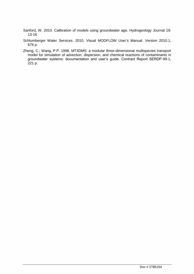
Figure 1. The domain of the western Lake Taupo catchment numerical model. The numbered polygons are surface water sub-catchments delineated by EW and numbers refer to sub- catchment names in Table 1.
Confidential 2011
GNS Science Report 2011/153 13
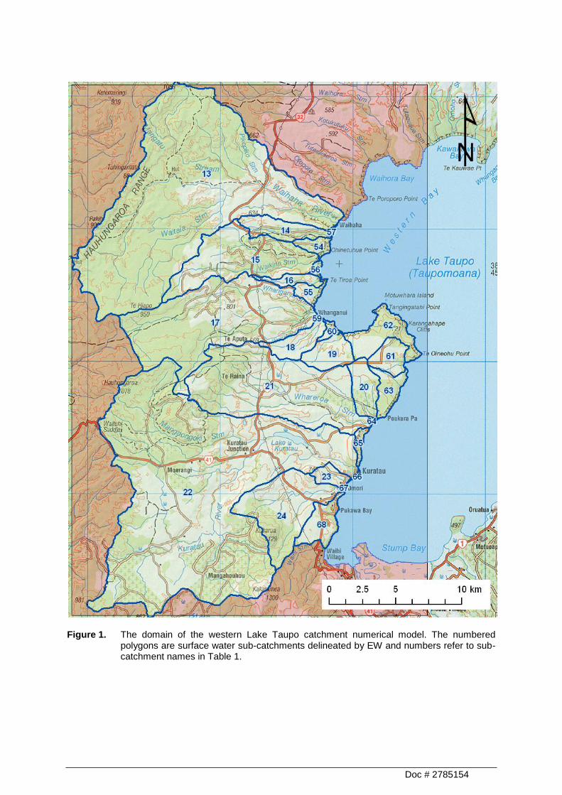
Figure 2. Cross sections at row 344 of the uniform 80 m wide by 20 m thick grid with 'A' unadjusted DTM and 'B' adjusted DTM. The upper grid, which was generated using an unadjusted DEM, has several areas where there is no lateral overlap along layers. The lower figure shows corrections (detailed in text) to drop elevations in cells that exceed 10 m difference from their lower elevation neighbours. This ensures that there is a minimum of 50% overlap between adjacent cells in each layer.
Doc # 2785154
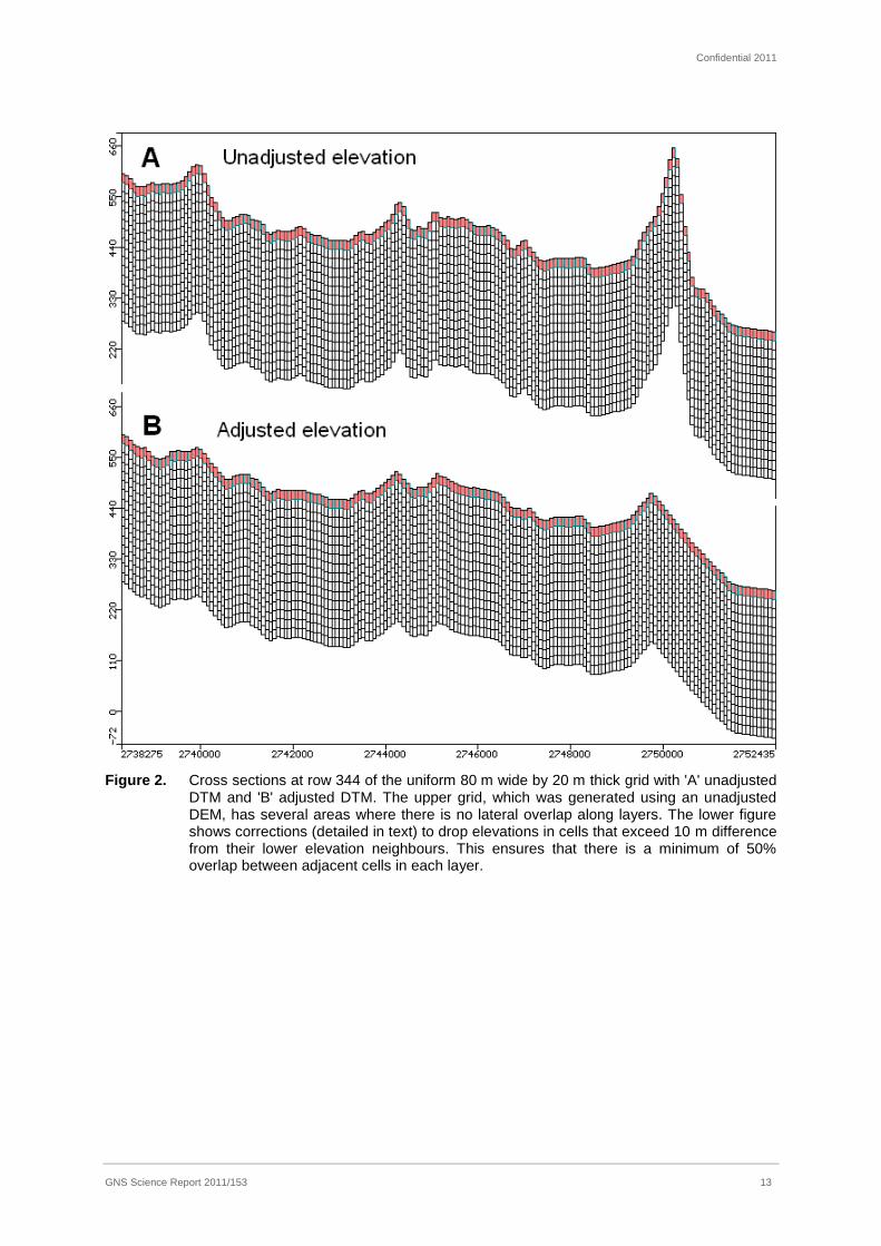
Figure 3. Plan view of model, showing the top layer of the hydrostratigraphy, where 'B2' is the greywacke basement unit, 'P7' is the Pakaumanu unit, 'W5' is the Whakamaru unit, and 'O3a' is the Oruanui unit. Grid cells that are not included in the groundwater flow and contaminant transport solution are marked as 'inactive cells'. Cross sections along rows 129, 186, 299, 330 and 429 are shown in Figure 4.
Confidential 2011
GNS Science Report 2011/153 15
Figure 4. Cross sections through model showing hydrostratigraphy of materials along rows 129, 186, 299, 330 and 429. Refer to Figure 3 for cross section locations and material names. Vertical exaggeration is 10 times.
Doc # 2785154
Figure 5. Boundary conditions (BC) for groundwater flow model, showing Lake Taupo simulated as a constant head BC, rivers/streams simulated as Cauchy head-dependant drain BCs, and annual groundwater recharge simulated as specified flux BC.
Confidential 2011
GNS Science Report 2011/153 17
Figure 6. Nitrate loading used as a constant concentration boundary condition on the topmost saturated cells or water table (Hadfield 2011). Cross sections along rows 129, 186, 299, 330 and 429 are used to report modelled nitrate concentrations in Figure 12.
Doc # 2785154
Figure 7. Zones used for ZONEBUDGET (ZBUD) to calibrate stream gauges. Zones are determined as the surface water catchment to each gauge location. Zone 1 is a default zone where no other zone has been specified, such as some parts of layer 1, and all of layers 2 to 16.
Confidential 2011
GNS Science Report 2011/153 19
Figure 8. Groundwater observation wells in the model domain used for groundwater flow model calibration (Gusyev et al. 2011).
Doc # 2785154
Figure 9. Simulated vs. observed stream/river flows, units are m³/s. Observed flows are represented with a vertical dashed line to show the minimum and maximum observed flows, while the middle symbol is represented by the median flow. Note that the simulated flows are within the min/max range for almost all gauging locations. The best-fit line has a slope of 0.9922 and R² of 0.9695.
0 1 2 3 4 5 6
01
23
45
6
Simulated flow
Ob
se
rve
d flo
w
1:1 line
min/max range
best fit line
Confidential 2011
GNS Science Report 2011/153 21
Figure 10. Calibration plot of modelled vs. observed hydraulic head in the steady-state groundwater flow model.
Doc # 2785154
Figure 11. Contour-fill map of groundwater table from steady-state flow simulation. Dry cells, and their layer number are overlaid, illustrating regions with a deep water table. The contour interval for the groundwater table elevation is 25 m, starting at 375 m. A light blue line shows the shoreline for the constant head boundary of 357 m for Lake Taupo.
Confidential 2011
GNS Science Report 2011/153 23
Figure 12. Cross sections showing groundwater flow and nitrate simulation results in mg/L. See Figure 4 for reference to hydrostratigraphy at the same locations in the model. The figures show the water table (thick blue line), with light grey regions of dry cells above (where applicable) to the top of the model. Within the saturated aquifer, shading and light-green contours show a log distribution of relative concentrations of nitrate after 80 years of simulation time. Arrows show relative groundwater flow velocities. Faded thick lines in the background show boundaries of hydrostratigraphy (same as Figure 4).

Doc # 2785154
TABLES
Confidential 2011
GNS Science Report 2011/153 25
Table 1. Data summary of 27 surface water sub-catchments in the western Lake Taupo catchment area (Gusyev et al. 2011).
No. Sub-catchment Name
Area, [km2] Average
recharge, [mm/year]
MRT, [years]
# of observation
wells
# of gauging stations
13 Waihaha River 155.443 890 49 1 6
14 Otaunga Stream 8.269 786 - 0 1
15 Waikino Stream 31.718 826 - 1 3
16 Te Awaroa
Stream 3.085
721 - 0 0
17 Whanganui
Stream 65.382
847 49 2 4
18 Orongopioi
Stream 6.886
683 - 0 0
19 Kotukutuku 2
Stream 7.309
602 - 2 0
20 Awatapu Stream 7.584 496 - 0 0
21 Whareroa
Stream 59.270
709 9 or 53 9 8
22 Kuratau River 199.571 985 30 6 4
23 Te Puke 3.187 568 - 0 0
24 Omori Stream 27.405 744 0.5 or 40 1 4
54 Ohinetuhua 2.752 684 - 0 0
55 Te Tawai 2.643 666 - 0 0
56 Te Papa 0.710 653 - 0 0
57 Taupo U6 0.224 639 - 0 0
58 Te Poroporo 2.963 644 - 0 0
59 Whekenui 0.122 622 - 0 0
60 Wharekaho 1.261 595 - 0 0
61 Te Hapua 5.690 459 - 0 0
62 Karangahape 11.059 487 - 0 0
63 Te Koromiko 5.466 441 - 0 0
64 Te Hape 0.160 458 - 0 0
65 Rangitukua 1.542 494 - 1 0
66 Te Rae 0.250 510 - 1 0
67 Taupo U7 0.051 533 - 0 0
68 Pukawa 7.373 636 - 0 0
"-" stands for "No available data".
Doc # 2785154
Table 2. Hydrogeologic properties of materials used for the model development model calibration.
Unit Code
Hydraulic conductivity value, [m/day] Calibrated Effective porosity Min Max Calibrated
Oruanui O3a 1.0 3.0 2.0 0.2
Whakamaru W5 0.04 0.3 0.02 0.1
Pakaumanu P7 0.03 0.06 0.04 0.05
Greywacke B2 0.01 0.01 0.01 0.05
Table 3. Steady-state groundwater flow budget, where 'IN' refers to water entering the groundwater domain and 'OUT' refers to water exiting the groundwater domain.
Zone ID
IN Flow Budget OUT Flow Budget
Recharge, [10³×
m³/day]
Fraction of total
recharge
Constant head, [10³×
m³/day]
Drains, [10³×
m³/day]
Fraction of
drains out
Constant head, [10³×
m³/day]
Zone 1 (remainder)
101.3 8.1% 0 81.7 6.7% 0
Zone 2 (Lake Taupo)
0.085 0.0% 16.6 10.0 0.8% 56.0
Zones 3-32 (Gauged)
1152.8 91.9% 0 1123.1 92.4% 0
Total 1254.2 100.0% 16.6 1214.8 100.0% 56.0
1270.8 1270.8