Embed Size (px)
Citation preview

Numerical Differential Equations
An Undergraduate Course
Ronald H.W. Hoppe

Contents
1. Ordinary Differential Equations 1
1.1 Initial-value Problems: Theoreticalfoundations and preliminaries 1
1.1.1 Basic definitions 1
1.1.2 Existence and uniqueness 3
1.1.3 Continuous Dependence on the initial data 4
1.1.4 Elementary examples of numerical integrators 6
1.1.5 Stiff and non-stiff systems 9
1.2 One-step methods for initial-valueproblems 13
1.2.1 Definitions 13
1.2.2 Convergence, consistency, and stability 13
1.2.3 Explicit Runge-Kutta methods 21
1.2.4 Asymptotic expansion of the globaldiscretization error 26
1.2.5 Explicit extrapolation methods 28
1.2.6 Adaptive step size control for explicitone-step methods 31
1.3 Multi-step methods 35
1.3.1 Basic definitions 35
1.3.2 Convergence, consistency, and stability 37
1.3.3 Extrapolatory and interpolatorymulti-step methods 45
1.3.4 Predictor-corrector methods 49
1.3.5 BDF (Backward Difference Formulas) 51

1.4 Numerical integration of stiff systems 52
1.4.1 Linear stability theory 52
1.4.2 A-stability, L-stability, and a(α)-stability 54
1.4.3 Implicit and semi-implicit Runge-Kutta methods 57
1.4.4 Linear multi-step methods and Dahlquist’ssecond barrier 61
1.4.5 A(α)-stability of implicit BDF 63
1.4.6 Numerical solution of differential-algebraic systems 64
1.5 Numerical solution of boundary-valueproblems 68
1.5.1 Theoretical foundations and preliminaries 68
1.5.2 Shooting methods 71
1.5.3 Finite difference approximations 75
1.5.4 Galerkin approximations 77
Literature 80

Partial Differential Equations 82
2.1 Theoretical foundations and preliminaries 82
2.2 Linear second order elliptic boundaryvalue problems 88
2.2.1 Preliminaries 88
2.2.2 Finite difference approximations 92
2.2.3 Sobolev spaces 99
2.2.4 Finite element approximations 104
2.3 The heat equation 126
2.3.1 Preliminaries 126
2.3.2 Method of lines and Rothe’s method 130
2.3.3 Finite difference approximations 131
2.3.4 Finite element approximations 136
2.4 The wave equation 140
2.4.1 Preliminaries 140
2.4.2 Finite difference approximations 144
2.4.3 Finite element approximations 147
Literature 152
Exercises 154
Numerical Differential Equations 1
1. Ordinary Differential Equations
1.1 Initial-value Problems: Theoretical foundations and pre-liminaries
1.1.1 Basic definitions
An ordinary differential equation is an equation which contains an un-known function in one independent variable along with certain deriva-tives of that function. The order of the differential equation corre-sponds to the highest derivative that occurs in the equation.
Definition 1.1. (First order system)(i) Assume that g : I × D1 × D2 → Rd, g = (g1, ..., gd)
T , where I :=[a, b] ⊂ R, Di ⊂ Rd, 1 ≤ i ≤ 2, and y : I → Rd, y = (y1, ..., yd)
T
with y′ = (y′1, ..., y′d)
T , y′i := dyidxi, 1 ≤ i ≤ d. Assume further that
(y(x), y′(x)) ∈ D1 ×D2, x ∈ I. Then
g(x, y(x), y′(x)) = 0 , x ∈ I,(1.1a)
is called a nonlinear system of ordinary differential equations of firstorder in implicit form.A function y ∈ C1(I)d satisfying (1.1a) is called a solution of the systemof ordinary differential equations of first order.(ii) Let α ∈ R
d, α = (α1, ..., αd)T , and assume that y ∈ C1(D) satisfies
(1.1a) and
y(a) = α.(1.1b)
Then, (1.1a),(1.1b) is called an initial value problem for the systemof ordinary differential equations of first order. (iii) Assume thatB : I × D → R
d×d, B = (Bij)di,j=1, D ⊂ R
d, and f : I × D → Rd, f =
(f1, ..., fd)T . Assume further that y : I → Rd as in (i) with y(x) ∈
D, x ∈ I. Then
B(x, y(x)) y′(x) = f(x, y(x)), x ∈ I,(1.2)
is called a quasilinear system of ordinary differential equations of firstorder in implicit form. In case B = B(y), f = f(y), the system (1.2) issaid to be autonomous.(iv) In the special case B = I we obtain
y′(x) = f(x, y(x)), x ∈ I.(1.3)
2 Ronald H.W. Hoppe
The system (1.3) is referred to as a system of ordinary differentialequations of first order in explicit form.(v) Assume that A,B : I → R
d×d, A = (Aij)di,j=1, B = (Bij)
di,j=1 and
f : I → Rd, f = (f1, ..., fd)T . Let further y be as in in (iii). Then
B(x) y′(x) = A(x) y(x) + f(x) , x ∈ I,(1.4a)
y′(x) = A(x) y(x) + f(x), x ∈ I,(1.4b)
are called linear systems of ordinary differential equations of first orderin implicit resp. explicit form.
Definition 1.2. (n-th order system)(i) Assume that g : I ×D → Rd, I := [a, b] ⊂ R, D ⊂ R(n+1)d, n ∈ N,and y : I → Rd with y(i)(x) := diy(x)/dxi, 1 ≤ i ≤ n. Assume furtherthat (y(x), y(1)(x), ..., y(n)(x))T ∈ D, x ∈ I. Then
g(x, y(x), y(1)(x), ..., y(n)(x)) = 0, x ∈ I,(1.5a)
is called a system of ordinary differential equations of n-th order inimplicit form.(ii) Assume that α ∈ Rnd, α = (α0, · · · , αn−1)
T , αi ∈ Rd, 0 ≤ i ≤ n−1.Moreover, suppose that
y(i)(a) = αi, 0 ≤ i ≤ n− 1.(1.5b)
Then, (1.5a),(1.5b) is called an initial value problem for the system ofordinary differential equations of n-th order. (iii) The definitions ofquasilinear resp. linear systems of n-th order and of systems of n-thorder in explicit form can be given analogously.
In the sequel we will restrict ourselves to systems of first order, sincehigher order equations can be equivalently written as a first order sys-tem as the following result shows.
Lemma 1.3. (Equivalence of n-th order equation and first or-der system)Any ordinary differential equation of n-th order is equivalent to a sys-tem of ordinary differential equations of first order.
Proof. Without restriction of generality we assume that d = 1 and thatthe ordinary differential equation of n-th order is explicit, i.e.,
y(n)(x) = f(x, y(x), y′(x), ..., y(n−1)(x)), x ∈ I.

Numerical Differential Equations 3
Setting yi(x) := y(i−1)(x), x ∈ I, 1 ≤ i ≤ n, there holds
y′1(x) = y2(x)y′2(x) = y3(x)· = ·
y′n−1(x) = yn(x)y′n(x) = f(x, y1(x), ..., yn−1(x))
,
i.e., (y1, ..., yn) satisfies a system of first order.
1.1.2 Existence and uniqueness
We consider an initial-value problem for a system of first order ordinarydifferential equations in explicit form. The continuity of the right-handside of the ordinary differential equation is sufficient for the existenceof a solution.
Theorem 1.4. (Peano’s existence theorem)Assume that I := [a, b] ⊂ R, D ⊂ R
d, f ∈ C(I×D), and α ∈ D. Then,the initial value problem
y′(x) = f(x, y(x)), x ∈ I,(1.6a)
y(a) = α(1.6b)
has a solution y ∈ C1(D).
However, the continuity of the right-hand side does not guaranteeuniqueness as the following example shows:
Example 1.5. (Non-uniqueness)We consider the initial-value problem
y′(x) =√
|y(x)|, x ∈ R,
y(2) = 1.
If y = y(x), x ∈ R is a solution, so is z(x) := −y(−x), i.e., it suffices toconsider positive solutions. Separation of variables results in
∫dy√y=
∫
dx =⇒ 2√y = x+ C =⇒ y(x;C) =
(x+ C)2
4.

4 Ronald H.W. Hoppe
The condition y(2) = 1 yields (C + 2)2 = 4 =⇒ C = 0. Multiplesolutions:
y(x; a) =
x2/4 , x > 00 , a ≤ x ≤ 0 (a ≤ 0)
− (x− a)2/4 , x < a
y(x) =
x2/4 , x > 0
0 , x ≤ 0.
If the right-hand side additionally satisfies a Lipschitz-condition in itssecond argument, we do have uniqueness.
Theorem 1.6. (Existence and uniqueness theorem of Picard-Lindelof)Assume that f : I × D → Rd, I := [a, b] ⊂ R, D ⊂ Rd, and α ∈ D.Assume further that
f ∈ C(I ×D),(1.7a)
and that there exists a constant L > 0 such that for all (x, yi) ∈ I ×D, 1 ≤ i ≤ 2, it holds
‖f(x, y1) − f(x, y2)‖ ≤ L ‖y1 − y2‖.(1.7b)
Then, the initial value problem (1.6a),(1.6b) has one and only one so-lution.
1.1.3 Continuous Dependence on the initial data
We study the continuous dependence of the solution on the initial data.
Lemma 1.7. (Gronwall’s lemma)Let Φ : I → R, I := [a, b] ⊂ R,Φ ∈ C(I), and assume that
Φ(x) ≤ α + β
x∫
a
Φ(s) ds, x ∈ I, α ≥ 0, β > 0.
Then, it holds
Φ(x) ≤ α exp(β (x− a)), x ∈ I.
Proof. Let ε > 0. We consider
Ψ(x) := (α + ε) exp(β (x− a)), x ∈ I =⇒ Ψ′(x) = β ψ(x)
=⇒ ψ(x) = ψ(a) + β
x∫
a
Ψ(s) ds.
Numerical Differential Equations 5
We show
Φ(x) < Ψ(x), x ∈ I.
Obviously, we have
Φ(a) ≤ α ≤ α + ε = Ψ(a).
In contradiction to the assertion we assume the existence of x ∈ (a, b]such that Φ(x) ≥ Ψ(x). Set
x0 := min x ∈ (a, b] | Φ(x) = Ψ(x) .We have Φ(x) ≤ Ψ(x), x ∈ [a, x0], whence
Φ(x0) ≤ α + β
x0∫
a
Φ(s) ds < α + ε+ β
x0∫
a
Ψ(s) ds = Ψ(x0)
contradicting the assumption Φ(x0) = Ψ(x0).
Theorem 1.8. (Continuous dependence on the initial data)Under the assumptions of the Theorem of Picard-Lindelof let yi, 1 ≤ i ≤2, two solutions of the system y′(x) = f(x, y(x)), x ∈ I, with respect tothe initial conditions yi(a) = αi. Then, it holds
‖y1(x) − y2(x)‖ ≤ ‖α1 − α2‖ exp(L(x− a)), x ∈ I.
Proof. In view of
yi(x) = αi +
x∫
a
f(s, yi(s)) ds, 1 ≤ i ≤ 2,
we have
‖y1(x)− y2(x)‖︸ ︷︷ ︸
=: Φ(x)
≤ ‖α1 − α2‖+x∫
a
‖f(s, y1(s))− f(s, y2(s))‖ ds ≤
‖α1 − α2‖︸ ︷︷ ︸
=: α
+ L︸︷︷︸
=: β
x∫
a
‖y1(s)− y2(s)‖︸ ︷︷ ︸
=: Φ(s)
ds.
Gronwall’s lemma allows to conclude.

6 Ronald H.W. Hoppe
1.1.4 Elementary examples of numerical integrators
We consider an initial-value problem for a scalar ordinary differentialequation of first order in explicit form
y′(x) = f(x, y(x)), x ∈ [a, b],
y(a) = α.
We introduce a partition of the interval I according to
Ih := a =: x0 < x1 < · · · < xN := b, N ∈ N,
with step sizes hk := xk+1 − xk, 0 ≤ k ≤ N − 1. The integration of thedifferential equation over the subinterval [xk, xk+1] yields
y(xk+1)− y(xk) =
xk+1∫
xk
f(x, y(x)) dx.(1.8)
The idea is to approximate the integral on the right-hand side by aquadrature formula.
Example 1.9. (Explicit and implicit Euler method)The integral on the right-hand side of (1.8) describes the area enclosedby the graph of the function f(·, y(·)) and the interval [xk, xk+1]. Inthe explicit Euler method it is approximated by the area of the rec-tangle [xk, xk+1] × [0, f(xk, y(xk))] (cf. Figure 1 left). In the implicitEuler method we approximate the integral by the area of the rectangle[xk, xk+1]× [0, f(xk+1, y(xk+1))] (cf. Figure 1 right).
x
f(x,y(x))
k+1xkx
y
x
y
f(x,y(x))
k+1xkx
Figure 1. The explicit (left) and the implicit (right)Euler method.
We replace the unknown function values y(xk) and y(xk+1) by someapproximations yk and yk+1 and thus obtain:

Numerical Differential Equations 7
(i) Explicit Euler method: For k = 0, 1, · · · , N − 1 compute
yk+1 = yk + hk f(xk, yk),(1.9a)
y0 = α.(1.9b)
We note that yk+1 can be explicitly computed by the evaluation of theright-hand side in (1.9a).
(ii) Implicit Euler method: For k = 0, 1, · · · , N − 1 compute
yk+1 = yk + hk f(xk+1, yk+1),(1.10a)
y0 = α.(1.10b)
We note that (1.10a) requires the solution of a nonlinear equation, i.e.,yk+1 is implicitly given.
Example 1.10. (Implicit trapezoidal rule)In the implicit trapezoidal rule the integral on the right-hand side of(1.8) is approximated by the area of the trapeze as depicted in Figure2:
xk+1∫
xk
f(x, y(x)) dx ≈ hk
(
f(xk, y(xk)) + f(xk+1, y(xk+1)))
.
x
f(x,y(x))
k+1xkx
y
Figure 2. The implicit trapezoidal rule.
Implicit trapezoidal rule: For k = 0, 1, · · · , N − 1 compute
yk+1 = yk + hk
(
f(xk, yk) + f(xk+1, yk+1))
,(1.11a)
y0 = α.(1.11b)

8 Ronald H.W. Hoppe
Example 1.11. (Explicit and implicit midpoint rule)In the explicit midpoint rule, the differential equation y′(x) = f(x, y(x))is integrated over the interval [xk, xk+2] resulting in
y(xk+2)− y(xk) =
xk+2∫
xk
f(x, y(x)) dx.
In the explicit midpoint rule we use a quadrature formula which approx-imates the integral by the area of the rectangle [xk, xk+2]× [0, f(xk+1,y(xk+1))] (cf. Figure 3 left):
xk+2∫
xk
f(x, y(x)) dx ≈ (hk + hk+1) f(xk+1, y(xk+1)).
In the implicit midpoint rule, the differential equation y′(x) = f(x, y(x))is integrated over the interval [xk, xk+1] and a quadrature formula isused which approximates the integral by the area of the rectangle[xk, xk+1]× [0, f(xk + hk/2, y(xk + hk/2))] (cf. Figure 3 right):
xk+1∫
xk
f(x, y(x)) dx ≈ hk f(xk + hk/2, y(xk + hk/2)).
Since we do not want to evaluate the function f at intermediate points,the function value f(xk + hk/2, y(xk + hk/2)) is approximated by thearithmetic mean of the function values with respect to xk and xk+1:
f(xk + hk/2, y(xk + hk/2)) ≈1
2
(
f(xk, yxk) + f(xk+1, y(xk+1))
)
.
y
xx k+1x k+2
f(x,y(x))
xk
x
f(x,y(x))
k+1xkx
y
Figure 3. The explicit (left) and the implicit (right)midpoint rule.
Numerical Differential Equations 9
Again, we replace the unknown function values y(xk), y(xk+1), andy(xk+2) by some approximations yk, yk+1, and yk+2. We note that theexplicit midpoint rule requires two start values y0 and y1. Given y0 = α,y1 can be computed, e.g., by the explicit Euler method. We thus obtain:
(i) Explicit midpoint rule: For k = 0, 1, · · · , N − 2 compute
yk+2 = yk + (hk + hk+1) f(xk, yk),(1.12a)
y0 = α, y1 = α + h0 f(a, α).(1.12b)
We note that yk+2 can be explicitly computed by the evaluation of theright-hand side in (1.12a).
(ii) Implicit midpoint rule: For k = 0, 1, · · · , N − 1 compute
yk+1 = yk +hk2
(
f(xk, yk) + f(xk+1, yk+1))
,(1.13a)
y0 = α.(1.13b)
We note that yk+1 is implicitly given, i.e., the computation requires thesolution of a nonlinear equation.
Remark 1.12. (Comparison of explicit and implicit methods)Since explicit methods only require function evaluations, whereas im-plicit methods require the solution of nonlinear equations and are thuscomputationally more expensive, the question is why one should useimplicit methods instead of explicit methods. The answer is that somesystems of ordinary differential equations require the solution by im-plicit methods as will be illustrated in the next subsection.
1.1.5 Stiff and non-stiff systems
A system of ordinary differential equations is called stiff, if the solutionhas components with extremely different growth behavior. Otherwise,it is said to be non-stiff.
Example 1.13. (Stiff system)We consider the following initial-value problem for a linear system offirst order
(y′1(x)y′2(x)
)
= − 1
2
(101 9999 101
)
︸ ︷︷ ︸
=: A
(y1(x)y2(x)
)
, x ≥ 0,
(y1(0)y2(0)
)
=
(20
)
.

10 Ronald H.W. Hoppe
We diagonalize the matrix A by a similarity transformation TAT ∗,where T := (e1|e2) with ei, 1 ≤ i ≤ 2, being the orthonormal eigenvec-tors associated with the eigenvalues λ1, λ2 of A:Computation of the eigenvalues of A as the zeroes of the characteristicpolynomial
det(λI − A) = λ2 − 101λ+ 100 =⇒ λ1 = 100 , λ2 = 1.
The orthonormal eigenvectors are given by
e1 =
( √2−1
√2−1
)
,
e2 =
( √2−1
−√2−1
)
.
Using the transformation matrix
T :=
( √2−1 √
2−1
√2−1 −
√2−1
)
,
(y1y2
)
= T
(y1y2
)
,
we obtain the transformed linear system(
T
(y1y2
))′
= −TAT ∗T
(y1y2
)
=⇒(y′1(x)y′2(x)
)
= −(
100 00 1
) (y1(x)y2(x)
)
, x ≥ 0,
(y1(0)y2(0)
)
=
( √2√2
)
.
It has the solution
y1(x) =√2 exp(−100x) , y2(x) =
√2 exp(−x).
The back transformation(y1y2
)
= T
(y1y2
)
results in
y1(x) = exp(−100x) + exp(−x) , y2(x) = exp(−100x)− exp(−x).The linear system is stiff, since the solution component exp(−100x)decays much faster than the solution component exp(−x).
We now consider the numerical solution of the initial-value problemfrom the example above with respect to an equidistant grid with grid
Numerical Differential Equations 11
points xk = kh, k ∈ N, h > 0, using the explicit Euler method. Theapplication of this method to the transformed linear system results in
y1,k = y1,k−1 − 100hy1,k−1 =
(1− 100h)y1,k−1 = (1− 100h)ky1,0,
y2,k = y2,k−1 − hy2,k−1 =
(1− h)y2,k−1 = (1− h)ky2,0.
The back transformation yields
y1,k = (1− 100h)k + (1− h)k,
y2,k = (1− 100h)k − (1− h)k.
We want that the approximate solution decays as the solution of thecontinuous problem, i.e., y1,k, y2,k → 0 for k → ∞. Hence, we musthave
|1− 100h| < 1 ⇐⇒ h <1
50.
On the other hand, we consider the numerical solution by the implicitEuler method. The application of this method to the transformed linearsystem gives
y1,k = y1,k−1 + 100hy1,k =⇒y1,k = (1 + 100h)−1y1,k−1 = (1 + 100h)−ky1,0,
y2,k = y2,k−1 + hy2,k =⇒y2,k = (1 + h)−1y2,k−1 = (1 + h)−ky2,0.
Transforming back, we obtain
y1,k = (1 + 100h)−k + (1 + h)−k,
y2,k = (1 + 100h)−k − (1− h)−k.
Obviously, we have y1,k, y2,k → 0 for k → ∞ without any restriction onthe step size h.
Remark 1.14. (Implicit methods for stiff systems)The application of the explicit and implicit Euler method to the stiffsystem from Example 1.13 shows that the explicit Euler method ismuch less suited than the implicit Euler method, since it requires thechoice of a very small step size to guarantee that the approximatesolution behaves in the same way as the exact solution. This does notonly yield a significant higher amount of computational work but alsomay lead to rounding errors. The next sections will show indeed that

12 Ronald H.W. Hoppe
explicit methods are well suited for non-stiff problems, whereas stiffproblems require the application of implicit schemes.

Numerical Differential Equations 13
1.2 One-step methods for initial-value problems
1.2.1 Definitions
We consider the initial-value problem
y′(x) = f(x, y(x)), x ∈ I := [a, b],(1.14a)
y(a) = α.(1.14b)
We assume f ∈ C(I × D), D ⊂ Rd, α ∈ D, and suppose that thereexists L ≥ 0 such that
‖f(x, y1) − f(x, y2)‖ ≤ L ‖y1 − y2‖(1.15)
for all (x, yi) ∈ I ×D , 1 ≤ i ≤ 2.
Definition 1.15. (Explicit and implicit one-step methods)Let Ih := xk = a + kh | 0 ≤ k ≤ N, N ∈ N, be an equidistantpartition of I = [a, b] of step size h = (b− a)/N and Φ : Ih× Ih× lRd×lRd × R+ → Rd. Then, the scheme
yk+1 = yk + h Φ(xk, xk+1, yk, yk+1, h), 0 ≤ k ≤ N − 1,(1.16a)
y0 = α(1.16b)
is called a one-step method with increment function Φ. The one-stepmethod is said to be explicit, if Φ does not depend on yk+1, and iscalled implicit otherwise.
Remark 1.16. (Interpretation as a difference equation)Setting I ′h := Ih \xN and introducing the grid function yh : Ih → Rd,the one-step method (1.16a),(1.16b) can be equivalent written as thedifference equation of first order
yh(x + h) = yh(x) + h Φ(x, x+ h, yh(x), yh(x+ h), h), x ∈ I ′h,
(1.17a)
yh(a) = α.(1.17b)
1.2.2 Convergence, consistency, and stability
Definition 1.17. (Convergence and order of convergence)The grid function
eh(x) := yh(x) − y(x), x ∈ Ih,(1.18)
is called the global discretization error. The one-step method (1.16a),(1.16b) is said to be convergent, if it holds
maxx∈Ih
‖eh(x)‖ → 0 (h→ 0).(1.19)

14 Ronald H.W. Hoppe
It is said to be convergent of order p, if
maxx∈Ih
‖eh(x)‖ = O(hp) (h→ 0).(1.20)
The convergence can be characterized by consistency and stability.Consistency guarantees that the one-step method (1.16a),(1.16b) is ameaningful approximation of the initial-value problem (1.14a),(1.14b).We can not expect that the exact solution y of the initial-value problemsatisfies the one-step method, but if we insert the exact solution intothe equivalent difference equation, we should have
y(x + h) − y(x)
h= h Φ(x, x+ h, y(x), y(x+ h), h),
↓ h→ 0 ↓ h→ 0
y′(x) f(x, y(x)).
Definition 1.18. (Consistency, order of consistency)The grid function
τh(x) := h−1 (y(x+ h) − y(x))− Φ(x, x+ h, y(x), y(x+ h), h),
is called the local discretization error. The one-step method (1.16a),(1.16b) is said to consistent with the initial-value problem (1.14a),(1.14b), if
h∑
x∈I′h
‖τh(x)‖ → 0 (h→ 0).(1.21)
It is said to be consistent of order p, if
h∑
x∈I′h
‖τh(x)‖ = O(hp) (h→ 0).(1.22)
Lemma 1.19. (Sufficient condition for consistency)Assume that
maxx∈I′h
‖τh(x)‖ → 0 (h→ 0).(1.23)
Then, the one-step method (1.16a),(1.16b) is consistent with the initial-value problem (1.14a),(1.14b).The condition (1.23) holds true if and only if
maxx∈I′h
‖Φ(x, x+ h, y(x), y(x+ h), h)− f(x, y(x))‖ → 0(1.24)
as h→ 0.
Proof. The proof is left as an exercise.

Numerical Differential Equations 15
Example 1.20. (Consistency order: explicit Euler method)The explicit Euler method reads
yh(x+ h) = yh(x) + h f(x, yh(x)) , yh(a) = α.
Hence, the local discretization error is given by
τh(x) = h−1 (y(x+ h) − y(x))− f(x, y(x)).
Taylor expansion leads
y(x+ h) = y(x) + h y′(x) +1
2h2 y′′(x) +O(h3) =⇒
h−1 (y(x+ h)− y(x)) = y′(x) +1
2h y′′(x) +O(h2) =
f(x, y(x)) +1
2h y′′(x) +O(h2).
It follows that
τh(x) =1
2h y′′(x) +O(h2).
Hence, if y ∈ C2(I), the explicit Euler method is consistent of orderp = 1.
Example 1.21. (Consistency order: implicit trapezoidal rule)The implicit trapezoidal rule reads
yh(x+ h) = yh(x) +h
2[f(x, yh(x)) + f(x+ h, yh(x+ h))], yh(a) = α.
By Taylor expansion we obtain
y(x+ h) = y(x) + h y′(x) +1
2h2 y′′(x) +
1
6h3 y′′′(x) +O(h4) =⇒
h−1 (y(x+ h)− y(x)) = y′(x) +1
2h y′′(x) +
1
6h2 y′′′(x) +O(h3) =⇒
h−1 (y(x+ h)− y(x)) = f(x, y(x)) +
1
2h (fx(x, y(x)) + fy(x, y(x)) f(x, y(x))) +
1
6h2 y′′′(x) +O(h3),
and
f(x+ h, y(x+ h)) = f(x, y(x)) + h fx(x, y(x)) +
h fy(x, y(x)) y′(x) +O(h2) =⇒
1
2(f(x, y(x)) + f(x+ h, y(x+ h))) = f(x, y(x)) +
1
2h (fx(x, y(x)) + fy(x, y(x)) f(x, y(x))) +O(h2).

16 Ronald H.W. Hoppe
It follows that
τh(x) = O(h2),
i.e., for y ∈ C3(I) the implicit trapezoidal rule if of consistency orderp = 2.
In contrast to the consistency which related the one-step method andthe initial-value problem, stability is alone a property of the one-stepmethod. It states the continuous dependence of the solution of theone-step method on its data.
We restrict ourselves to the explicit one-step method
yh(x+ h) = yh(x) + h Φ(x, yh(x), h),(1.25a)
yh(a) = α.(1.25b)
Definition 1.22. (Asymptotic stability)Consider the perturbed one-step method
zh(x+ h) = zh(x) + h(
Φ(x, zh(x), h) + σh(x))
,(1.26a)
zh(a) = α+ βh.(1.26b)
The explicit one-step method (1.25a),(1.25b) is called asymptoticallystable, if there exist hmax > 0 and for each ε > 0 a number δ > 0 suchthat for all perturbations σh, βh with
‖βh‖+ h∑
x∈I′h(x)
‖σh(x)‖ < δ
for h < hmax the solutions of the perturbed one-step method (1.26a),(1.26b) satisfy
maxx∈Ih
‖(yh − zh)(x)‖ + h∑
x∈I′h
‖(Dhyh − Dhzh)(x)‖ < ε,
where (Dhyh)(x) := h−1 (yh(x+ h)− yh(x)), x ∈ I ′h.
A significant tool in the proof of the continuous dependence of theexact solution on the initial data was Gronwall’s lemma (cf. Lemma1.7). A discrete analog of Gronwall’s lemma will play a prominentrole in the proof of the asymptotic stability of the one-step method(1.25a),(1.25b).

Numerical Differential Equations 17
Lemma 1.23. (Discrete Gronwall’s lemma)Consider a grid function vh : Ih → Rd with vj := vh(xj), 0 ≤ j ≤ N,and assume that there exist δ ≥ 0 and η ≥ 0 such that
‖vj+1‖ ≤ δ h
j∑
k=0
‖vk‖+ η, 0 ≤ j ≤ N − 1,(1.27a)
‖v0‖ ≤ η,(1.27b)
hold true. Then we have
‖vj‖ ≤ η exp(δ (xj − a)), 0 ≤ j ≤ N.(1.28)
Proof. Suppose that ‖vj‖ ≤ M, 0 ≤ j ≤ N . By induction we provethat
‖vj‖ ≤Mδm (xj − a)m
m!+ η
m−1∑
ℓ=0
δℓ (xj − a)ℓ
ℓ!.(1.29)
(i) Induction basis: Obviously, the assertion (1.28) holds true for j =0, m ∈ N, and m = 0, 0 ≤ j ≤ N .(ii) Induction assumption: The assertion (1.28) holds true for somem ∈ N and 0 ≤ j ≤ N .(iii) Induction conclusion: We have
‖vj+1‖ ≤ δ h
j∑
k=0
(
Mδm (xk − a)m
m!+ η
m−1∑
ℓ=0
δℓ (xk − a)ℓ
ℓ!
)
+ η.
Using the elementary inequality
h
j∑
k=0
(xk − a)ℓ ≤xj+1∫
a
(x− a)ℓ dx =(xj+1 − a)ℓ+1
ℓ+ 1,
for m+ 1 and j + 1 we obtain
‖vj+1‖ ≤Mδm+1 (xj+1 − a)m+1
(m+ 1)!+ η
m∑
ℓ=0
δℓ (xj+1 − a)ℓ
ℓ!.
Theorem 1.24. (Sufficient condition for asymptotic stability)Assume that the increment function Φ satisfies the following Lips-chitz condition: There exist a neighborhood U ⊂ I × D of the graph(x, y(x)) | x ∈ I of the exact solution y of the initial-value problem

18 Ronald H.W. Hoppe
and numbers hmax > 0 and LΦ ≥ 0 such that for all 0 < h < hmax andall (x, yi) ∈ U, 1 ≤ i ≤ 2, it holds
‖Φ(x, y1, h)− Φ(x, y2, h)‖ ≤ LΦ ‖y1 − y2‖.(1.30)
Then, for all perturbations σh, βh with
‖βh‖+ h∑
x∈Ih
‖σh(x)‖ ≤ δ
and x ∈ Ih resp. x ∈ I ′h the solution yh of the unperturbed one-stepmethod (1.25a),(1.25b) and the solution zh of the perturbed one-stepmethod (1.26a),(1.26b) satisfy
‖(yh − zh)(x)‖ ≤(
‖βh‖+ h∑
x∈Ih
‖σh(x)‖)
exp(LΦ(x− a)),(1.31a)
‖(Dhyh −Dhzh)(x)‖ ≤ LΦ ‖(yh − zh)(x)‖+ ‖σh(x)‖.(1.31b)
In particular, this implies asymptotic stability of the one-step method(1.25a),(1.25b).
Proof. Without restriction of generality let U = I ×D. We set
wh(x) := zh(x)− yh(x), x ∈ Ih.
With wj := wh(xj) it follows that
wj+1 = wj + h(
Φ(xj , zj, h) + σj − Φ(xj , yj, h))
, w0 = βh =⇒
wj+1 = w0 + h
j∑
k=0
(
σk + Φ(xk, zk, h)− Φ(xk, yk, h))
.
The Lipschitz condition (1.30) yields
‖wj+1‖ ≤ ‖βh‖+ h
N∑
k=0
‖σk‖+ LΦ h
j∑
k=0
‖wk‖.
Then, the discrete Gronwall’s lemma implies (1.31a). The assertion(1.31b) is a direct consequence of (1.31a) and
(Dhwh)(x) = Φ(x, zh(x), h) + σh(x)− Φ(x, yh(x), h).
An important result is that consistency and asymptotic stability of theone-step method (1.25a),(1.25b) implies convergence with the order ofconvergence being the order of consistency.

Numerical Differential Equations 19
Theorem 1.25. (Consistency and stability imply convergence)
Assume that the one-step method (1.25a),(1.25b) is consistent with theinitial-value problem (1.14a),(1.14b) and asymptotically stable. Thenit holds
maxx∈Ih
‖(yh − y)(x)‖ → 0 (h→ 0),(1.32a)
∑
x∈I′h
‖(Dhyh −Dhy)(x)‖ → 0 (h→ 0).(1.32b)
Proof. We set zh(x) := y(x), x ∈ Ih. It follows that σh(x) = τh(x)and βh = 0. In view of the consistency, for each ε > 0 there existhmax(ε) > 0 and δ(ε) > 0 such that for 0 < h < hmax(ε) we have
h∑
x∈I′h
‖τh(x)‖ < δ(ε).
The asymptotic stability implies (1.32a),(1.32b).
Theorem 1.26. (Characterization of convergence)Assume that the one-step method (1.25a),(1.25b) satisfies the Lipschitzcondition (1.30). Then, the following two statements are equivalent:
(i) The one-step method (1.25a),(1.25b) is convergent and (1.32a),(1.32b) hold true.
(ii) The one-step method (1.25a),(1.25b) is consistent with the initial-value problem (1.14a),(1.14b).
For consistent one-step methods there exists hmax > 0 such that for all0 < h < hmax the following a priori error estimate holds true:
‖(yh − y)(x)‖ ≤ (h∑
x∈I′h
‖τh(x)‖) exp(LΦ (x− a)).(1.33)
If additionally maxx∈I′h
‖τh(x)‖ → 0 (h→ 0) is satisfied, then we have
maxx∈I′h
‖(Dhyh −Dhy)(x)‖ → 0 (h→ 0).(1.34)
Proof. We first show that (ii) implies (i). Theorem 1.24 gives theasymptotic stability of the one-step method and Theorem 1.25 im-plies convergence in the sense of (1.32a),(1.32b). The a priori estimate(2.90) and (1.34) follow from Theorem 1.24 with zh(x) := y(x) so thatσh(x) = τh(x) and βh = 0.
20 Ronald H.W. Hoppe
Next, we show that (i) implies (ii). In view of the convergence, forsufficiently small h the Lipschitz condition (1.30) can be applied to
Φ(x, yh(x), h)− Φ(x, y(x), h),
whence
‖τh(x)‖ = ‖Dhy(x)− Φ(x, y(x), h)‖ =
‖(Dh)y(x)− Φ(x, y(x), h)−Dhyh(x) + Φ(x, yh(x), h)‖ ≤‖(Dhyh −Dhy)(x)‖+ LΦ ‖(yh − y)(x)‖.
Multiplication by h and summation over x ∈ I ′h allows to conclude.
Remark 1.27. (Implicit one-step methods)The definition of asymptotic stability can be generalized to implicitone-step methods. The corresponding stability and convergence resultshold true as well.
Remark 1.28. (Lipschitz condition for the increment function)
If the increment function Φ only involves the right-hand side f of theinitial-value problem, the Lipschitz condition (1.30) follows from thecorresponding Lipschitz condition for f .
Numerical Differential Equations 21
1.2.3 Explicit Runge-Kutta methods
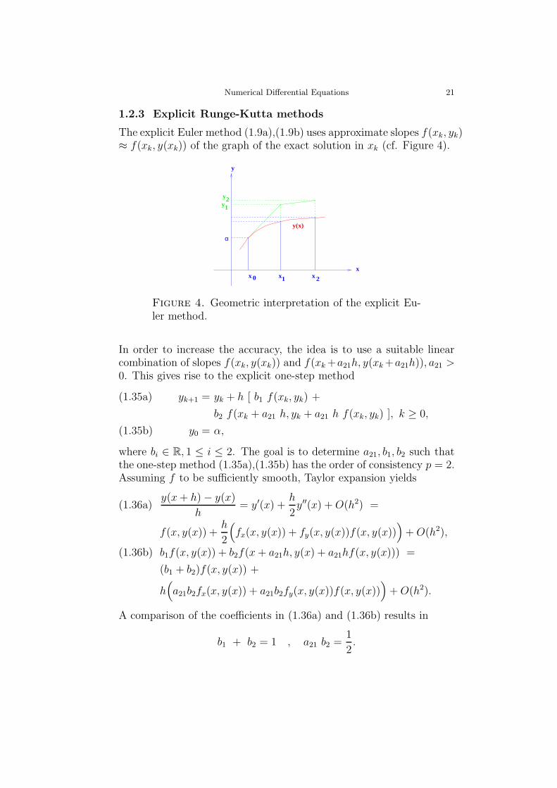
The explicit Euler method (1.9a),(1.9b) uses approximate slopes f(xk, yk)≈ f(xk, y(xk)) of the graph of the exact solution in xk (cf. Figure 4).
x
y
x xx1 2
y(x)
0
α
y1
y2
Figure 4. Geometric interpretation of the explicit Eu-ler method.
In order to increase the accuracy, the idea is to use a suitable linearcombination of slopes f(xk, y(xk)) and f(xk+a21h, y(xk+a21h)), a21 >0. This gives rise to the explicit one-step method
yk+1 = yk + h [ b1 f(xk, yk) +(1.35a)
b2 f(xk + a21 h, yk + a21 h f(xk, yk) ], k ≥ 0,
y0 = α,(1.35b)
where bi ∈ R, 1 ≤ i ≤ 2. The goal is to determine a21, b1, b2 such thatthe one-step method (1.35a),(1.35b) has the order of consistency p = 2.Assuming f to be sufficiently smooth, Taylor expansion yields
y(x+ h)− y(x)
h= y′(x) +
h
2y′′(x) +O(h2) =(1.36a)
f(x, y(x)) +h
2
(
fx(x, y(x)) + fy(x, y(x))f(x, y(x)))
+O(h2),
b1f(x, y(x)) + b2f(x+ a21h, y(x) + a21hf(x, y(x))) =(1.36b)
(b1 + b2)f(x, y(x)) +
h(
a21b2fx(x, y(x)) + a21b2fy(x, y(x))f(x, y(x)))
+O(h2).
A comparison of the coefficients in (1.36a) and (1.36b) results in
b1 + b2 = 1 , a21 b2 =1
2.

22 Ronald H.W. Hoppe
Choosing β := b2 gives
b1 = 1− β , a21 =1
2β.
Definition 1.29. (Method of Runge and Heun)The explicit one-step method
yk+1 = yk + (1− β) h f(xk, yk) +(1.37a)
β h f(xk +1
2βh, yk +
h
2βf(xk, yk)), k ≥ 0,
y0 = α,(1.37b)
is called the method of Runge. In particular, for the special choiceβ = 1
2it is called the method of Heun.
We now study the question whether by a suitable choice of β we canachieve an order of consistency p = 3. To this end we determine afurther term in the Taylor expansion:
y(x+ h)− y(x)
h= y′(x) +
h
2y′′(x) +
h2
6y′′′(x) +O(h3) =
f +h
2[fx + fyf ] +
h2
6
(
fxx + 2ffxy + f 2fyy + fxfy + ff 2y
)
+O(h3),
(1− β)f(x, y(x)) + βf(x+h
2β, y(x) +
h
2βf(x, y(x))) =
f +h
2
(
fx + fyf)
+h2
8β
(
fxx + 2ffxy + f 2fyy
)
+O(h3).
Again, a comparison of coefficients yields
τh(x) =h2
6
(
(1− 3
4β) (fxx + 2ffxy + f 2fyy) + fxfy + ff 2
y
)
+O(h3).
Hence, the consistency order p = 3 can not be achieved by any choiceof β. However, if we choose β = 3
4, the sum of the coefficients in front
of the leading error term of τh is minimized.
The construction of the method of Runge can be generalized and givesrise to explicit Runge-Kutta methods of higher order.
Numerical Differential Equations 23
Definition 1.30. (Explicit s-stage Runge-Kutta method)The explicit one-step method
yk+1 = yk +
s∑
j=1
bj kj , k ≥ 0,(1.38a)
y0 = α,(1.38b)
with
k1 := h f(xk, yk),
k2 := h f(xk + a21h, yk + a21k1),
k3 := h f(xk + a31h+ a32h, yk + a31k1 + a32k2),
·· · · · · · · · · · · · · · · · · · · · · · · · · · · · · · · · · · · · ·
ki := h f(xk + cih, yk +i−1∑
j=1
aijkj), ci :=i−1∑
j=1
aij , 1 ≤ i ≤ s,
is called an explicit s-stage Runge-Kutta method. It is uniquely deter-mined by the s(s + 1)/2 parameters aij, 2 ≤ i ≤ s, 1 ≤ j ≤ i − 1, andbi, 1 ≤ i ≤ s.
An explicit s-stage Runge-Kutta method can be described by the so-called Butcher scheme
c1 = 0 a21c2 a31 a32· · · ·· · · · ·· · · · · ·cs as1 as2 · · as,s−1
b1 b2 · · bs−1 bs
Lemma 1.31. (Consistency of s-stage Runge-Kutta methods)Under the assumption
s∑
i=1
bi = 1(1.39)
the explicit s-stage Runge-Kutta method (1.38a),(1.38b) is consistentwith the initial-value problem (1.14a),(1.14b).
24 Ronald H.W. Hoppe
Proof. For the local discretization error we obtain
τh(x) =y(x+ h)− y(x)
h−
s∑
i=1
bi f(x+ cih, y(x) +i−1∑
j=1
aijkj),
where kj is given as in (1.38a) with yk replaced by y(x). For h → 0 itfollows that
τh(x) → y′(x)−s∑
i=1
bi f(x, y(x)) = y′(x)− f(x, y(x)) = 0.
The goal is to determine the parameters aij and bi in such a way thatthe highest possible consistency order p can be achieved. This can berealized by graph-theoretical concepts (Butcher trees). For details werefer to the textbooks by Butcher and Hairer/Norsett/Wanner.The following table contains the number N(s) of parameters to bedetermined and the number M(s) of equations to be satisfied as wellas the maximal achievable consistency order p(s):
s 1 2 3 4 5 6 7 8 9 10Ns 1 3 6 10 15 21 28 36 45 55Ms 1 2 4 8 17 37 85 200 486 1205ps 1 2 3 4 4 5 6 6 7 8
If M(s) < N(s), the ’free’ parameters are chosen such that the leadingterm in the local discretization error gets minimized.
Example 1.32. (Kutta’s third order method)The 4 equations to be satisfied by the 6 unknown parameters are givenby
b1 + b2 + b3 = 1 ,
b2 a21 + b3 (a31 + a32) =1
2,
b2 a221 + b3 (a231 + 2 a31 a32 + a232) =
1
3,
b3 a32 a21 =1
6.
The associated Butcher scheme reads

Numerical Differential Equations 25
0 0 0 012
12
0 01 −1 2 0
16
23
16
Example 1.33. (Classical fourth order Runge-Kutta method)The Butcher scheme for the classical fourth order Runge-Kutta methodis given by
0 0 0 0 012
12
0 0 012
0 12
0 01 0 0 1 0
16
13
13
16
26 Ronald H.W. Hoppe
1.2.4 Asymptotic expansion of the global discretization error
An asymptotic expansion of the global discretization error is a prereq-uisite for extrapolation methods that will be treated in the subsequentsubsection.
We assume that the explicit one-step method (1.25a),(1.25b) has con-sistency order p. Then, the local discretization error admits the as-ymptotic expansion
y(x+ h)− y(x)− h Φ(x, y(x), h) =(1.40)
dp+1(x) hp+1 + dp+2(x) h
p+2 + · · · .A natural question is whether the global discretization error has a sim-ilar asymptotic expansion.
Theorem 1.34. (Theorem of Gragg)Let f ∈ Cp+k(I × D) and let Φ ∈ Cp+k(I × D × lR+), k ≥ 1, be theincrement function of an explicit one-step method with Φ(x, y, 0) =f(x, y), (x, y) ∈ I × D. Moreover, assume that there exist functionsdp+i ∈ Ck−i(I), 1 ≤ i ≤ k, such that the local discretization errorsatisfies
y(x+ h)− y(x)− h Φ(x, y(x), h) =
k∑
i=1
dp+i(x) hp+i +O(hp+k+1),
where x ∈ I ′h. Then, the global discretization error admits the asymp-totic expansion
eh(x) =k−1∑
i=0
ep+i(x) hp+i + Ep+k(x; h) h
p+k, x ∈ Ih.
Here, the coefficient functions ep+i, 0 ≤ i ≤ k − 1, are solutions of thelinear initial-value problems
e′p+i(x) = fy(x, y(x)) ep+i(x)− dp+i+1(x), x ∈ I,
ep+i(a) = 0.
Further, there exist hmax > 0 and a constant C > 0, independent of h,such that
‖Ep+k(x; h)‖ ≤ C, x ∈ Ih, 0 < h < hmax.
Remark 1.35. (Implicit one-step methods)Gragg’s theorem can be generalized to implicit one-step methods. How-ever, the iterative solution of the associated nonlinear system of equa-tions may perturb the asymptotic expansion.

Numerical Differential Equations 27
Example 1.36. (Asymptotic expansions of the explicit/implicitEuler method)The explicit and the implicit Euler methods (1.9a),(1.9b), and (1.10a),(1.10b) admit asymptotic expansions of the globaldiscretization error in h.
Particular interest is on one-step methods that admit an asymptoticexpansion of the global discretization error in h2.
Theorem 1.37. (Theorem of Stetter)Assume that the one-step method
yh(x+ h) = yh(x) + h Φ(x, x+ h, yh(x), yh(x+ h), h), x ∈ I ′h,
yh(a) = α,
is symmetric, i.e.,
Φ(x, x+ h, yh(x), yh(x+ h), h) = Φ(x+ h, x, yh(x+ h), yh(x),−h).Under the assumptions of Theorem 1.34 it holds
e2m+1(x) = 0, x ∈ I,
i.e., there exists an asymptotic expansion of the global discretizationerror in h2.
Example 1.38. (Explicit midpoint rule)Although the explicit midpoint rule (cf. Example 1.11) formally is atwo-step method, it can be equivalently written as a system of twoone-step methods to which the assumptions of Theorem 1.37 apply.Hence, the explicit midpoint rule admits an asymptotic expansion ofthe global discretization error in h2.

28 Ronald H.W. Hoppe
1.2.5 Explicit extrapolation methods
We consider an explicit one-step method (1.25a),(1.25b) which admitsan asymptotic expansion of the global discretization error in hγ.
Example 1.39. (Extrapolation in case of an asymptotic expan-sion in h)In Theorem 1.34 we assume p = 1, γ = 1. For the step sizes h and h/2we obtain
yh(x)− y(x) = e1(x) h+ E2(x; h) h2,(1.41a)
yh/2(x)− y(x) =1
2e1(x) h+
1
4E2(x; h) h
2.(1.41b)
Multiplication of (1.41b) with 2 and subtraction of (1.41a) yield
(2 yh/2(x)− yh(x))︸ ︷︷ ︸
=:yh(x)
−y(x) = O(h2).
Now, consider the polynomial p1 ∈ P1(R) with p1(hi) = yhi(x), 1 ≤ i ≤
2, where h1 := h and h2 := h/2. We obtain
p1(t) =2
h(yh(x)− yh/2(x)) (t−
h
2) + yh/2(x) =⇒
p1(0) = 2 yh/2(x)− yh(x) = yh(x).
Hence, the construction of the approximation yh(x) of order h2 corre-
sponds to an extrapolation to the step size h = 0.
Example 1.40. (Extrapolation in case of an asymptotic expan-sion in h) In Theorem 1.34 we assume p = 2, γ = 2. For the step sizesh and h/2 we obtain
yh(x)− y(x) = e2(x) h2 + E4(x; h) h
4,(1.42a)
yh/2(x)− y(x) =1
4e2(x) h
2 +1
16E4(x; h) h
4.(1.42b)
Multiplication of (1.42b) with 4 and subtraction of (1.42a) implies
4 yh/2(x)− 3 yh(x) = O(h4) =⇒4 yh/2(x)− 3 yh(x)
3︸ ︷︷ ︸
=:yh(x)
−y(x) = O(h4).

Numerical Differential Equations 29
We consider the polynomial p1 ∈ P1(R) in t2 with p1(hi) = yhi
(x), 1 ≤i ≤ 2, where h1 := h and h2 := h/2. It follows that
p1(t2) =
4
3h2(yh(x)− yh/2(x)) (t
2 − h2
4) + yh/2(x) =⇒
p1(0) =4
3yh/2(x)−
1
3yh(x) = yh(x).
Again, the construction of the approximation yh(x) of order h4 corre-
sponds to an extrapolation to the step size h = 0.
In practice, more than two step sizes are used for extrapolation:Given a basic step size H > 0, we choose a step size sequence
hi := H/ni, ni ∈ N, i = 1, 2, ...,(1.43)
characterized by the sequence
F := n1, n2, ...,and compute the approximations
y(H ; hi) := yhi, i = 1, 2, ....
The associated sequence Ti,1 = y(H ; hi), i = 1, 2, ..., forms the first col-umn of an extrapolation tableau. In case of polynomial extrapolationof Aitken-Neville type we determine a polynomial in hγ
Tik(h) := a0 + a1 hγ + ...+ ak−1 h
(k−1)γ ,
such that
Tik(hj) := y(H ; hj), j = i, i− 1, ..., i− k + 1,
and extrapolate to h = 0: Tik := Tik(0). This gives rise to the recursion
Tik = Ti,k−1 +Ti,k−1 − Ti−1,k−1
( ni
ni−k+1)γ − 1
, i ≥ k, k ≥ 2.
The extrapolation tableau looks as follows:
y(H ; h1) : T11y(H ; h2) : T21 T22y(H ; h3) : T31 T32 T33
· : · · · ·· : · · · · ·
y(H ; hi) : Ti1 Ti2 Ti3 · · Tii

30 Ronald H.W. Hoppe
Common choices of the step size sequence are given by:
(i) Harmonic sequence
ni = i, i ∈ N,
FH = 1, 2, 3, 4, 5, ....(ii) Romberg sequence
ni = 2i, i ∈ N,
FR = 2, 4, 8, 16, 32, ....(iii) Bulirsch sequence
ni =
3 · 2(i−2)/2, i even
2(i+1)/2, i odd,
FB = 2, 3, 4, 6, 8, 12, 16, ....

Numerical Differential Equations 31
1.2.6 Adaptive step size control for explicit one-step methods
Let yk+1 be an approximation computed by an explicit one-step methodof order p:
yk+1 = yk + h Φ(xk, yk, h).
We are looking for an easily computable a posteriori estimator for theglobal discretization error
ek+1 := yk+1 − y(xk+1).
Lemma 1.41. (Error estimator)Assume that yk+1 is a more accurate approximation of y(xk+1) accord-ing to
‖yk+1 − y(xk+1)‖ ≤ q ‖yk+1 − y(xk+1)‖, 0 ≤ q < 1.
Then
εk+1 := ‖yk+1 − yk+1‖is an estimator of ek+1 in the sense that
1
1 + qεk+1 ≤ ‖ek+1‖ ≤ 1
1− qεk+1.
Proof. The assertions can be easily deduced by an application of theright- and left-hand side of the triangle inequality.
We now assume that yk+1 is an approximation of y at xk+1 of orderp+ 1, i.e.,
‖yk+1 − y(xk+1)‖ ≤ C hp+1.
Given a prespecified accuracy ε > 0, for a ’reasonable’ new step sizeh := xk+2 − xk+1 we should have
C hp+1 .= ρ ε.(1.44)
where 0 < ρ < 1 represents a ’safety factor’. If yk+1 satisfies
εk+1 := ‖yk+1 − yk+1‖ .= ε
.= C hp+1,
then C.= εk+1/h
p+1. Inserting into (1.44) and solving for h yields
h = h (ρ ε
εk+1)1/(p+1).
There are two strategies to determine yk+1:
(i) extrapolation,
(ii) embedded Runge-Kutta methods of higher order.
32 Ronald H.W. Hoppe
We first consider extrapolation: Let yk+1 and yk+1 be the approxima-tions associated with the step sizes h and h/2, i.e.,
yk+1 − y(xk+1).= C hp,(1.45a)
yk+1 − y(xk+1).= C (
h
2)p = 2−p C hp.(1.45b)
Subtraction of (1.45b) from (1.45a) yields
yk+1 − yk+1.= C hp (1− 2−p) = C hp
2p − 1
2p,
and hence,
C.=
2p − 1
2ph−p (yk+1 − yk+1).
If we insert C into (1.45b) and solve for y(xk+1), we obtain
yk+1 = yk+1 +yk+1 − yk+1
2p − 1.
Embedded Runge-Kutta methods of higher order are based on Runge-Kutta-Fehlberg methods: Let yk+1 be an approximation of y(xk+1)obtained by an explicit s-stage Runge-Kutta method of order p:
yk+1 = yk +
s∑
i=1
bi ki,
ki = h f(xk + ci h, yk +
i−1∑
j=1
aij kj),
ci =
i−1∑
j=1
aij.
We compute yk+1 as the solution of an explicit (s+ t)-stage ’embedded’Runge-Kutta method of order p + 1:
yk+1 = yk +s+t∑
i=1
bi ki,
ki = h f(xk + ci h, yk +i−1∑
j=1
aij kj),
ci =i−1∑
j=1
aij.
The Butcher scheme of the embedded (s+t)-stage Runge-Kutta methodreads
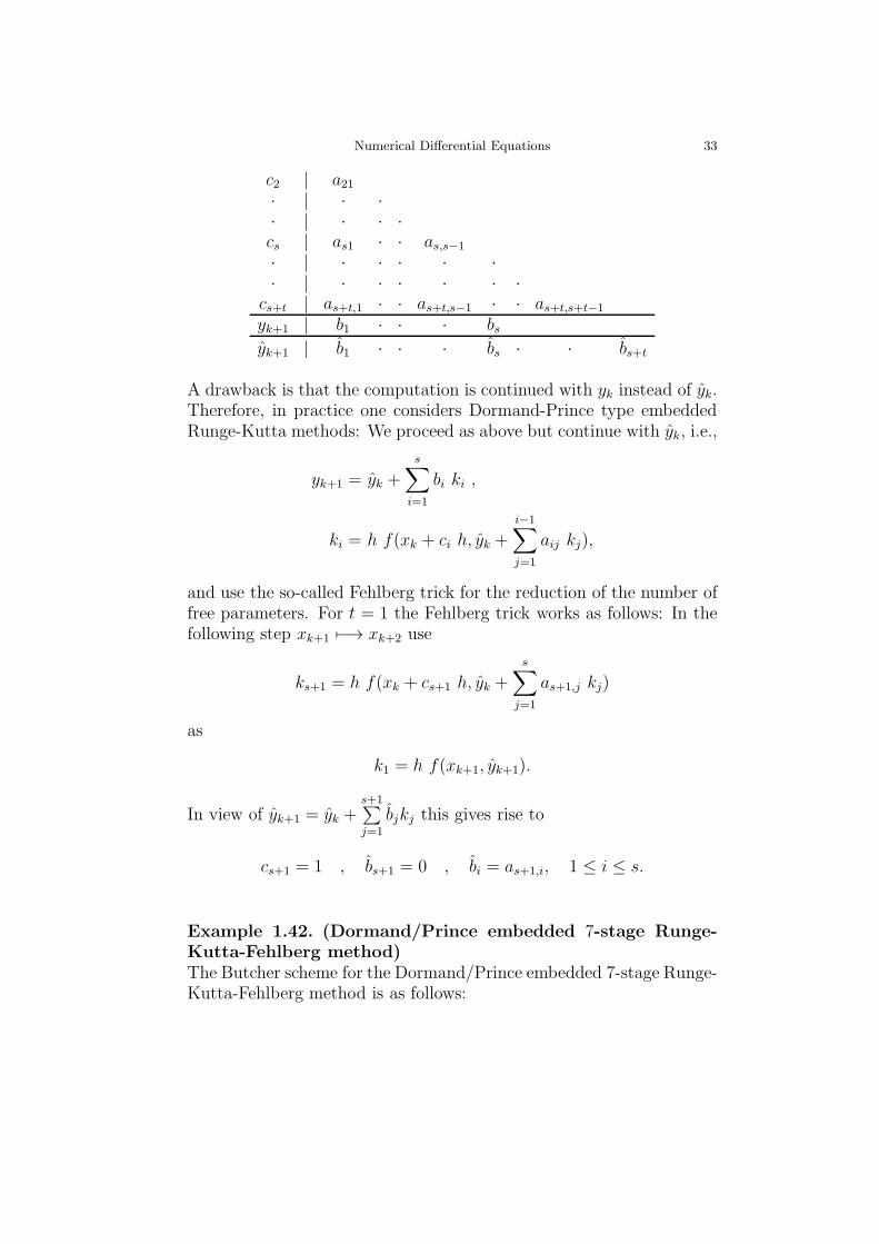
Numerical Differential Equations 33
c2 | a21· | · ·· | · · ·cs | as1 · · as,s−1
· | · · · · ·· | · · · · · ·
cs+t | as+t,1 · · as+t,s−1 · · as+t,s+t−1
yk+1 | b1 · · · bsyk+1 | b1 · · · bs · · bs+t
A drawback is that the computation is continued with yk instead of yk.Therefore, in practice one considers Dormand-Prince type embeddedRunge-Kutta methods: We proceed as above but continue with yk, i.e.,
yk+1 = yk +
s∑
i=1
bi ki ,
ki = h f(xk + ci h, yk +
i−1∑
j=1
aij kj),
and use the so-called Fehlberg trick for the reduction of the number offree parameters. For t = 1 the Fehlberg trick works as follows: In thefollowing step xk+1 7−→ xk+2 use
ks+1 = h f(xk + cs+1 h, yk +s∑
j=1
as+1,j kj)
as
k1 = h f(xk+1, yk+1).
In view of yk+1 = yk +s+1∑
j=1
bjkj this gives rise to
cs+1 = 1 , bs+1 = 0 , bi = as+1,i, 1 ≤ i ≤ s.
Example 1.42. (Dormand/Prince embedded 7-stage Runge-Kutta-Fehlberg method)The Butcher scheme for the Dormand/Prince embedded 7-stage Runge-Kutta-Fehlberg method is as follows:

34 Ronald H.W. Hoppe
0
15
15
310
340
940
45
4445
−5615
329
89
193726561
−253602187
644486561
−212729
1 90173168
−35533
467325247
49176
− 510318656
1 35384
0 5001113
125192
−21876784
1184
35384
0 5001113
125192
−21876784
1184
0
517957600
0 757116695
393640
− 92097339200
1872100
140

Numerical Differential Equations 35
1.3 Multi-step methods
1.3.1 Basic definitions
In the sequel we will use the grid-point sets
Ih := xj = a + j h | 0 ≤ j ≤ N, h := (b− a)/N,
I ′h := xj ∈ Ih | m ≤ j ≤ N , m ≥ 2.
Definition 1.43. (Multi-step method)Given real numbers α0, α1, · · · , αm, αm 6= 0, a function Φ : Ih×Rd(m+1)×R+ → Rd and vectors α(0), · · · , α(m−1) ∈ Rd, the scheme
1
h
m∑
k=0
αk yj+k = Φ(xj+m, yj, ..., yj+m; h), 0 ≤ j ≤ N −m,(1.46a)
yj = α(j), 0 ≤ j ≤ m− 1,(1.46b)
is called a multi-step method. The multi-step method is said to beexplicit, if Φ(x, z0, ..., zm; h) does not depend on zm, and implicit oth-erwise.Using the grid function yh : Ih → Rd, the multi-step method (1.46a),(1.46b) can be written as a difference equation of m-th order:
1
h
m∑
k=0
αk yh(x+ kh) = Φ(x+mh, yh(x), ..., yh(x+mh); h),(1.47a)
yh(a+ jh) = α(j), 0 ≤ j ≤ m− 1.(1.47b)
Example 1.44. (Milne-Simpson method)For the scalar first order ordinary differential equation
y′(x) = f(x, y(x)), x ∈ [a, b],
integration over [xk, xk+2] ⊂ [a, b] yields
y(xk+2)− y(xk) =
xk+2∫
xk
f(x, y(x)) dx.
Approximating the right-hand side by the Simpson rule, we obtain theMilne-Simpson rule
yk+2 = yk +h
3
(
f(xk, yk) + 4 f(xk+1, yk+1) + f(xk+2, yk+2))
.

36 Ronald H.W. Hoppe
Definition 1.45. (Linear multi-step methods)If there exist real numbers β0, β1, · · · , βm, such that the function Φ isgiven by
Φ(x, z0, · · · , zm; h) =m∑
k=0
βk f(xk, zk), xm ∈ I ′h,
the multi-step method (1.46a),(1.46b) is said to be a linear multi-stepmethod.
Remark 1.46. (Start ramp)For j > 1 the determination of the initial vectors α(j), 0 ≤ j ≤ m− 1,can be done by a multi-step method of a lower step number. This iscalled the start ramp.
Definition 1.47. (Characteristic polynomials)For a multi-step method (1.46a),(1.46b) the polynomial
ρ(z) :=
m∑
k=0
αk zk
is called the characteristic polynomial of the multi-step method.In case of a linear multi-step method, we can assign another character-istic polynomial associated with the increment function Φ:
σ(z) :=m∑
k=0
βk zk.

Numerical Differential Equations 37
1.3.2 Convergence, consistency, and stability
Definition 1.48. (Convergence and convergence order)If y ∈ C1([a, b]) is the exact solution of the initial-value problem(1.6a),(1.6b) and yh : Ih → Rd is the approximation obtained bythe multi-step method (1.46a),(1.46b), again we denote by eh(x) :=yh(x) − y(x), x ∈ Ih, the global discretization error. The solution yhof the multi-step method (1.46a),(1.46b) is said to convergence to thesolution y of the initial-value problem, if
maxx∈Ih
‖eh(x)‖ → 0 (h→ 0).
The multi-step method (1.46a),(1.46b) is said to convergence of orderp > 0, if there exists a constant C > 0, independent of h, such that
maxx∈Ih
‖eh(x)‖ ≤ C hp (h→ 0).(1.48)
As in the case of one-step methods, the convergence of multi-step meth-ods can be characterized by consistency and stability.
Definition 1.49. (Consistency and order of consistency)Let y ∈ C1([a, b]) be the exact solution of the initial-value problem(1.6a),(1.6b). Then, the grid function
τh(x) :=1
h
m∑
k=0
αk y(x− (m− k)h)− Φ(x, y(x−mh), · · · , y(x); h),
τh(xj) := y(xj)− α(j), 0 ≤ j ≤ m− 1,
is called the local discretization error of the multi-step method (1.46a),(1.46b).The multi-step method is said to be consistent with the initial-valueproblem, if
max0≤j≤m−1
|τh(xj)|+ h∑
x∈I′h
|τh(x)| → 0 (h→ 0).
The multi-step method has the order of consistency p > 0, if thereexists a constant C > 0, independent of h, such that
max0≤j≤m−1
|τh(xj)|+ h∑
x∈I′h
|τh(x)| ≤ C hp (h→ 0).(1.49)
38 Ronald H.W. Hoppe
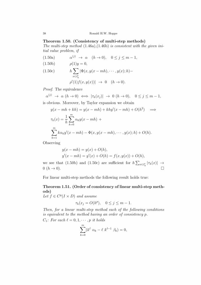
Theorem 1.50. (Consistency of multi-step methods)The multi-step method (1.46a),(1.46b) is consistent with the given ini-tial value problem, if
α(j) → α (h→ 0), 0 ≤ j ≤ m− 1,(1.50a)
ρ(1)y = 0,(1.50b)
h∑
x∈I′h
|Φ(x, y(x−mh), · · · , y(x); h)−(1.50c)
ρ′(1)f(x, y(x))| → 0 (h→ 0).
Proof. The equivalence
α(j) → α (h→ 0) ⇐⇒ |τh(xj)| → 0 (h→ 0), 0 ≤ j ≤ m− 1,
is obvious. Moreover, by Taylor expansion we obtain
y(x−mh+ kh) = y(x−mh) + khy′(x−mh) +O(h2) =⇒
τh(x) =1
h
m∑
k=0
αky(x−mh) +
m∑
k=1
kαky′(x−mh)− Φ(x, y(x−mh), · · · , y(x); h) +O(h).
Observing
y(x−mh) = y(x) +O(h),
y′(x−mh) = y′(x) +O(h) = f(x, y(x)) +O(h),
we see that (1.50b) and (1.50c) are sufficient for h∑
x∈I′h|τh(x)| →
0 (h→ 0).
For linear multi-step methods the following result holds true:
Theorem 1.51. (Order of consistency of linear multi-step meth-ods)Let f ∈ Cp(I ×D) and assume
τh(xj = O(hp), 0 ≤ j ≤ m− 1.
Then, for a linear multi-step method each of the following conditionsis equivalent to the method having an order of consistency p.
C1: For each ℓ = 0, 1, · · · , p it holdsm∑
k=0
(kℓ αk − ℓ kℓ−1 βk) = 0,

Numerical Differential Equations 39
C2: z = 0 is a zero of order ≥ p+ 1 of the entire function
ϕ(z) := ρ(exp(z))− z σ(exp(z)).
C3: The initial-value problem
y′(x) = y(x), x ∈ I , y(a) = 1,
has the order of consistency p.
C4: The order of consistency is p for a class of initial-value problemswhose solutions span the linear space of polynomials of degree p.
Proof. We first prove the equivalence of C1 and C4. We note thatf ∈ Cp(I ×D) implies y ∈ Cp+1(I). Taylor expansion yields
h τh(x+mh) =
m∑
k=0
(
αk y(x+ kh)− hβk f(x+ kh, y(x+ kh))︸ ︷︷ ︸
= y′(x+kh)
)
,
y(x+ kh) = y(x) +
p∑
ℓ=1
1
ℓ!kℓ hℓ y(ℓ)(x) +O(hp+1),
y′(x+ kh) =
p−1∑
ℓ=0
1
ℓ!kℓ hℓ y(ℓ+1)(x) +O(hp) =
p∑
ℓ=1
1
(ℓ− 1)!kℓ−1 hℓ−1 y(ℓ)(x) +O(hp) =⇒
h τh(x+mh) =(1.51)
m∑
k=0
(
αk y(x) +
p∑
ℓ=1
(αk
ℓ!kℓ − βk
(ℓ− 1)!kℓ−1) hℓ y(ℓ)(x)
)
+O(hp).
It follows that
C1 =⇒ |τh(x+mh)| = O(hp).
Conversely, the consistency order p implies C1, if in (1.51) we use thefunctions y = 1, y = x, · · · , y = xp.The equivalence of C4 can be shown similarly.
We next show the equivalence of C3. If the linear multi-step methodis consistent of order p, then C3 obviously holds true. Conversely,assume that C3 is satisfied. Inserting y(x) = exp(x−a) into (1.51) and

40 Ronald H.W. Hoppe
summing over Ih yields
h τh(x+mh)︸ ︷︷ ︸
= O(hp)
=
p∑
ℓ=0
1
ℓ!
( m∑
k=0
(kℓ αk − ℓ kℓ−1 βk))
hℓ−1∑
x+mh∈Ih
h exp(x− a)
︸ ︷︷ ︸
→b∫
aexp(x−a)dx (h→0)
︸ ︷︷ ︸
= O(hp)
+O(hp)
=⇒m∑
k=0
(kℓ αk − ℓ kℓ−1 βk) = 0, 0 ≤ ℓ ≤ p.
Finally, we prove the equivalence of C2. Taylor expansion of ϕ(z)around z = 0 results in
ϕ(z) = ρ(exp(z))− z σ(exp(z)) =
p∑
ℓ=0
ϕ(ℓ)(0) zℓ +O(hp) =⇒
ϕ(ℓ)(0) = 0 ⇐⇒m∑
k=0
(kℓ αk − ℓ ℓ−1 βk) = 0, 0 ≤ ℓ ≤ p.
For the stability of the multi-step method (1.47a),(1.47b) we considerthe linear space C(Ih) of grid functions on Ih equipped with the norm
|||zh||| :=m−1∑
j=0
|zh(xj)|+ h∑
x∈I′h
|zh(x)|.
The multi-step method define a mapping
Ah : C(Ih) → C(Ih)
Ahzh(xj) :=
zj − α(j) , 0 ≤ j ≤ m− 1,
1h
m∑
k=0
αk zj−m+k − Φ(xj , zj−m, · · · , zj, h) , m ≤ j ≤ N.
Definition 1.52. (Local Lipschitz stability of multi-step meth-ods)The multi-step method (1.47a),(1.47b) is said to be locally Lipschitz
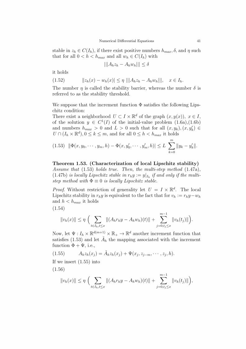
Numerical Differential Equations 41
stable in zh ∈ C(Ih), if there exist positive numbers hmax, δ, and η suchthat for all 0 < h < hmax and all wh ∈ C(Ih) with
|||Ahzh − Ahwh||| ≤ δ
it holds
‖zh(x)− wh(x)| ≤ η |||Ahzh −Ahwh|||, x ∈ Ih.(1.52)
The number η is called the stability barrier, whereas the number δ isreferred to as the stability threshold.
We suppose that the increment function Φ satisfies the following Lips-chitz condition:There exist a neighborhood U ⊂ I × R
d of the graph (x, y(x)), x ∈ I,of the solution y ∈ C1(I) of the initial-value problem (1.6a),(1.6b)and numbers hmax > 0 and L > 0 such that for all (x, yk), (x, y
′k) ∈
U ∩ (Ih × Rd), 0 ≤ k ≤ m, and for all 0 ≤ h < hmax it holds
‖Φ(x, y0, · · · , ym, h)− Φ(x, y′0, · · · , y′m, h)| ≤ Lm∑
k=0
‖yk − y′k‖.(1.53)
Theorem 1.53. (Characterization of local Lipschitz stability)Assume that (1.53) holds true. Then, the multi-step method (1.47a),(1.47b) is locally Lipschitz stable in rhy := y|Ih if and only if the multi-step method with Φ ≡ 0 is locally Lipschitz stable.
Proof. Without restriction of generality let U = I × Rd. The localLipschitz stability in rhy is equivalent to the fact that for vh := rhy−wh
and h < hmax it holds
‖vh(x)‖ ≤ η( ∑
t∈Ih,t≤x
‖(Ahrhy −Ahwh)(t)‖+m−1∑
j=0,tj≤x
‖vh(tj)‖)
.
(1.54)
Now, let Ψ : Ih ×Rd(m+1) ×R+ → Rd another increment function thatsatisfies (1.53) and let Ah the mapping associated with the incrementfunction Φ + Ψ, i.e.,
Ahzh(xj) = Ahzh(xj) + Ψ(xj, zj−m, · · · , zj , h).(1.55)
If we insert (1.55) into
‖vh(x)‖ ≤ η( ∑
t∈Ih,t≤x
‖(Ahrhy −Ahwh)(t)‖+m−1∑
j=0,tj≤x
‖vh(tj)‖)
,
(1.56)
42 Ronald H.W. Hoppe
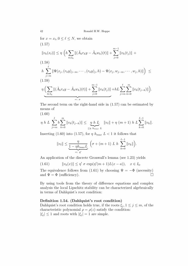
for x = xℓ, 0 ≤ ℓ ≤ N, we obtain
‖vh(xℓ)‖ ≤ η(
h∑
t∈Ih
‖(Ahrhy − Ahwh)(t)‖+m−1∑
j=0
‖vh(tj)‖ +
(1.57)
h
ℓ∑
j=m
‖Ψ(xj, (rhy)j−m, · · · , (rhy)j, h)−Ψ(xj , wj−m, · · · , wj, h)‖)
≤
(1.58)
η(∑
t∈Ih
‖(Ahrhy − Ahwh)(t)‖+m−1∑
j=0
‖vh(tj)‖︸ ︷︷ ︸
=: σ
+hL
ℓ∑
j=m
m∑
k=0
‖vh(tj−k)‖)
.
(1.59)
The second term on the right-hand side in (1.57) can be estimated bymeans of
η h Lℓ∑
j=m
bm∑
k=0
‖vh(tj−k)‖ ≤ η h L︸ ︷︷ ︸
≤η hmax L
‖vℓ‖+ η (m+ 1) h Lℓ−1∑
k=0
‖vk‖.
(1.60)
Inserting (1.60) into (1.57), for η hmax L < 1 it follows that
‖vℓ‖ ≤ η
1− ηhmaxL︸ ︷︷ ︸
=: η′
(
σ + (m+ 1) L hℓ−1∑
k=0
‖vk‖)
.
An application of the discrete Gronwall’s lemma (see 1.23) yields
‖vh(x)‖ ≤ η′ σ exp(η′(m+ 1)L(x− a)), x ∈ Ih.(1.61)
The equivalence follows from (1.61) by choosing Ψ = −Φ (necessity)and Ψ = Φ (sufficiency).
By using tools from the theory of difference equations and complexanalysis the local Lipschitz stability can be characterized algebraicallyin terms of Dahlquist’s root condition:
Definition 1.54. (Dahlquist’s root condition)Dahlquist’s root condition holds true, if the roots ξj, 1 ≤ j ≤ m, of thecharacteristic polynomial ρ = ρ(z) satisfy the condition:|ξj| ≤ 1 and roots with |ξj| = 1 are simple.

Numerical Differential Equations 43
Theorem 1.55. (Algebraic characterization of Lipschitz stabil-ity)Under the assumption (1.53), Dahlquist’s root condition is necessaryand sufficient for the local Lipschitz stability of the multi-step method(1.47a),(1.47b) in rhy.
As in the case of one-step methods, consistency and stability implyconvergence.
Theorem 1.56. (Convergence of multi-step methods)Under the Lipschitz condition (1.53) assume that the multi-step method(1.47a),(1.47b) is consistent with the initial-value problem (1.6a),(1.6b) andLipschitz stable in rhy with the stability barrier η > 0. Then, thereexist numbers hmax > 0 and δ > 0 such that for all 0 ≤ h < hmax theequation Ahyh = gh is uniquely solvable in U for all gh ∈ C(Ih) with|||gh||| < δ and the a priori estimate
maxx∈Ih
‖(yh − y)(x)‖ ≤ η(
|||gh|||+ |||τh|||)
(1.62)
holds true. In particular, for gh ≡ 0 we have
maxx∈Ih
‖yh(x)− y(x)‖ → 0 (h→ 0).
The order of convergence corresponds to the order of consistency.
Proof. Without restriction of generality we assume U = I×Rd. In view
of the Lipschitz continuity of the increment function Φ, the Banachfixed point theorem implies the existence of a solution yh ∈ C(Ih).Choosing zh := yh and wh := rhy, the Lipschitz stability with stabilitybarrier η implies that for 0 ≤ h < hmax
‖yh(x)− y(x)‖ ≤ η |||gh − τh|||, x ∈ Ih.(1.63)
The consistency yields |||τh||| → 0(h → 0) so that yh is uniquely de-termined for sufficiently small h and δ. The estimate (1.62) followsreadily from (1.63).
There is an upper bound on the achievable order of convergence of alocally Lipschitz stable linear multi-step method, known as Dahlquist’sfirst barrier.
44 Ronald H.W. Hoppe
Theorem 1.57. (Dahlquist’s first barrier)For the order of convergence p of a locally Lipschitz stable linear multi-step method it holds
p ≤
m+ 2 , if m is even,m+ 1 , if m is odd,
m , if it is explicit.
Stable multi-step methods of order m+ 2 are symmetric, i.e.,
αk = − αm−k, 0 ≤ k ≤ m,
βk = βm−k, 0 ≤ k ≤ m.
Numerical Differential Equations 45
1.3.3 Extrapolatory and interpolatory multi-step methods
Extrapolatory and interpolatory linear multi-step methods can be con-structed by numerical quadrature: The idea is to integrate y′(x) =f(x, y(x)) over [x∗, x+mh]
y(x+mh) = y(x∗) +
x+mh∫
x∗
f(s, y(s)) ds
and to replace the integrand by an interpolating polynomial of degreer with respect to the interpolation points
(x+ jh, f(x+ jh, y(x+ jh)), 0 ≤ j ≤ r,
where r = m (interpolation) or r = m− 1 (extrapolation):
Type Name r x∗
Extrapolatory Adams-Bashforth m− 1 x+ (m− 1)hmethod Nystrom m− 1 x+ (m− 2)h
Interpolatory Adams-Moulton m x+ (m− 1)hmethod Milne-Simpson m x+ (m− 2)h
(i): Adams-Bashforth method
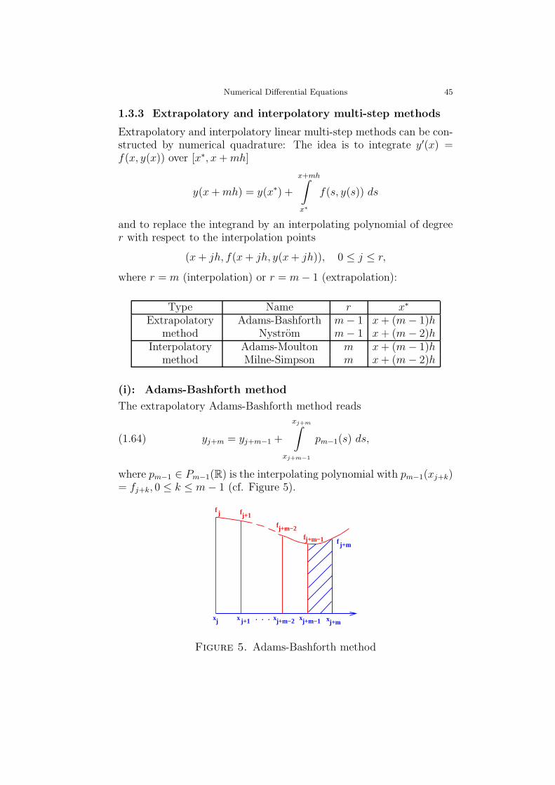
The extrapolatory Adams-Bashforth method reads
yj+m = yj+m−1 +
xj+m∫
xj+m−1
pm−1(s) ds,(1.64)
where pm−1 ∈ Pm−1(R) is the interpolating polynomial with pm−1(xj+k)= fj+k, 0 ≤ k ≤ m− 1 (cf. Figure 5).
xj+m−2.. x.xj x j+1 x
j+1f j
f j+m
f
j+m−1 j+m
fj+m−1
fj+m−2
Figure 5. Adams-Bashforth method
46 Ronald H.W. Hoppe
Newton’s representation of the interpolating polynomial is as follows:
pm−1(s) =
m−1∑
k=0
(−1)k (−tk ) ∇kfj+m−1,(1.65)
where t = 1h(s − xj+m−1) and ∇kfℓ = ∇k−1fℓ − ∇k−1fℓ−1. Inserting
(1.65) into (1.64) yields
yj+m = yj+m−1 +
m−1∑
k=0
(−1)k
xj+m∫
xj+m−1
(−tk ) ds ∇kfj+m−1.(1.66)
Setting
γk := (−1)k1
h
xj+m∫
xj+m−1
(−tk ) ds =
︸︷︷︸
Subst. t=h−1(s−xj+m−1)
(−1)k1∫
0
(−tk ) dt,
from (1.66) we obtain the Adams-Bashforth method in the form
yj+m = yj+m−1 + h
m−1∑
k=0
γk ∇kfj+m−1, 0 ≤ j ≤ N −m,(1.67a)
yk = α(k), 0 ≤ k ≤ m− 1.(1.67b)
Lemma 1.58. (Recursion formula for the Adams-Bashforthmethod)The coefficients γk, 0 ≤ k ≤ m − 1, of the Adams-Basforth method(1.67a),(1.67b) can be computed by means of the recursion formula
γk +1
2γk−1 +
1
3γk−2 + · · ·+ 1
k + 1γ0 = 1.
Proof. The proof follows from the relationship
∞∑
k=0
(−1)k1∫
0
(−tk ) dt z
k = − (1− z)−t
log(1− z)|t=1
t=0.
Theorem 1.59. (Convergence of the Adams-Bashforth method)
Assume y ∈ Cm(I) and suppose that f : I ×D → Rd satisfies a Lips-chitz condition. Then, the Adams-Bashforth method (1.67a),(1.67b) islocally Lipschitz stable and consistent of order m. The order of con-vergence corresponds to the order of consistency.

Numerical Differential Equations 47
An equivalent formulation of the Adams-Bashforth method can be de-rived by an evaluation of the differences ∇kfj+m−1. It reads
yj+m = yj+m−1 + hm−1∑
k=0
αmk fj+k, 0 ≤ j ≤ N −m,(1.68a)
yk = α(k), 0 ≤ k ≤ m− 1,(1.68b)
where the coefficients αmk, 0 ≤ k ≤ m− 1, are given by
αmk =
m−1∑
ℓ=m−k−1
γℓ (−1)m−k−1 (ℓm−k−1).
(ii): Adams-Moulton method
The interpolatory Adams-Moulton method reads
yj+m = yj+m−1 +
∫
xj+m−1
xj+mpm(s) ds(1.69)
where pm ∈ Pm(R) is the interpolating polynomial with pm(xj+k) =fj+k, 0 ≤ k ≤ m (cf. Figure 6).
xj+m−2.. x.xj x j+1 x
j+1f j
fj+m
f
j+m−1 j+m
fj+m−1
fj+m−2
Figure 6. Adams-Moulton method
Here, Newton’s representation of the interpolating polynomial reads
pm(s) =m∑
k=0
(−1)k (−tk ) ∇kfj+m.(1.70)
48 Ronald H.W. Hoppe
Inserting (1.70) into (1.69) yields
yj+m = yj+m−1 + hm∑
k=0
νk ∇kfj+m, 0 ≤ j ≤ N −m,(1.71a)
yk = α(k), 0 ≤ k ≤ m− 1,(1.71b)
νk := (−1)k0∫
−1
(−tk ) dt, 0 ≤ k ≤ m.(1.71c)
Lemma 1.60. (Recursion formula for the Adams-Moultonmethod)The coefficients νk, 0 ≤ k ≤ m, of the Adams-Moulton method (1.71a)-(1.71c) satisfy the recursion formula
νk +1
2νk−1 +
1
3νk−2 + · · ·+ 1
k + 1ν0 = 0.
Theorem 1.61. (Convergence of the Adams-Moulton method)
Assume y ∈ Cm+1(I) and suppose that f : I × D → Rd satisfies aLipschitz condition. Then, for h sufficiently small the Adams-Moultonmethod (1.71a)-(1.71c) is well defined. It is locally Lipschitz stable andconsistent of order m+1. The order of convergence corresponds to theorder of consistency.
By an evaluation of the differences ∇kfj+m we obtain the followingequivalent formulation of the Adams-Moulton method
yj+m = yj+m−1 + h
m∑
k=0
βmk fj+k, 0 ≤ j ≤ N −m,(1.72a)
yk = α(k), 0 ≤ k ≤ m− 1,(1.72b)
where the coefficients βmk, 0 ≤ k ≤ m, are given by
βmk := (−1)m−km∑
ℓ=m−k
νℓ (ℓ
m−k), 0 ≤ k ≤ m.
Remark 1.62. (Nystrom and Milne-Simpson method)Nystrom’s method and the method of Milne-Simpson can be derivedsimilarly.
Numerical Differential Equations 49
1.3.4 Predictor-corrector methods
Extrapolatory (explicit) multi-step methods have the advantage thatthey are computationally cheap and the disadvantage that the order ofconvergence is lower than corresponding interpolatory (implicit) meth-ods. On the other hand, for interpolatory (implicit) methods the ad-vantage of a higher order of convergence is marred by the fact thatthey are computationally more expensive. Predictor-corrector meth-ods combine the advantages and avoid the disadvantages.
The idea is to compute an approximate solution based on an interpo-latory multi-step method by fixed point iteration and to use a startiterate computed by an extrapolatory multi-step method:
(i) P : Predictor (e.g. Adams-Bashforth method)
y(0)j+m = yj+m−1 + h
m−1∑
k=0
αmk fj+k.
(ii) E : Evaluate
f(0)j+m := f(xj+m, y
(0)j+m).
(iii) C : Corrector (e.g. Adams-Moulton method)
y(1)j+m = yj+m−1 + h βmm f
(0)j+m + h
m−1∑
k=0
βmk fj+k.
Variants of the predictor-corrector methods
I. P (EC)ℓE method
(a) y(0)j+m = y
(ℓ)j+m−1 + h
m−1∑
k=0
αmk f(ℓ)j+k,
(b)f(r−1)j+m = f(xj+m, y
(r−1)j+m )
y(r)j+m = y
(ℓ)j+m−1 + h βmm f
(r−1)j+m + h
m−1∑
k=0
βmk f(ℓ)j+k
1 ≤ r ≤ ℓ,
(c) f(ℓ)j+m = f(xj+m, y
(ℓ)j+m).
50 Ronald H.W. Hoppe
II. P (EC)ℓ method
(a) y(0)j+m = y
(ℓ)j+m−1 + h
m−1∑
k=0
αmk f(ℓ−1)j+k ,
(b)f(r−1)j+m = f(xj+m, y
(r−1)j+m )
y(r)j+m = y
(ℓ)j+m−1 + h βmm f
(r−1)j+m + h
m−1∑
k=0
βmk f(ℓ−1)j+k
1 ≤ r ≤ ℓ.
Numerical Differential Equations 51
1.3.5 BDF (Backward Difference Formulas)
The idea behind the Backward Difference Formulas (BDF) is to usethe interpolating polynomial
pm ∈ Pm(R) , pm(xj+k) = yj+k), 0 ≤ k ≤ m,
for the approximation of y′(x) = f(x, y(x)) in xj+m−r, r = 0 or r = 1:
p′m(xj+m−r) = f(xj+m−r, yj+m−r).
Newton’s representation of the interpolating polynomial
pm(x) =
m∑
k=0
(−1)k (−tk ) ∇kyj+m , t := (x − xj+m)/h
yields
p′m(xj+m−r) =1
h
m∑
k=0
ρrk ∇kyj+m = f(xj+m−r, yj+m−r),(1.73a)
ρrk = (−1)kd
dt(−t
k )|t=−r , 0 ≤ k ≤ m.(1.73b)
Remark 1.63. (Implicit/explicit BDF)For r = 0 we obtain an implicit method, whereas r = 1 yields anexplicit method. For r = 0 it follows that
ρ00 = 0, ρ0k =1
k, 1 ≤ k ≤ m.

52 Ronald H.W. Hoppe
1.4 Numerical integration of stiff systems
1.4.1 Linear stability theory
For linear systems y′ = Ay the growth behavior of the solutions isdetermined by the eigenvalues λ ∈ σ(A), where σ(A) stands for thespectrum of the matrix A. For nonlinear autonomous systems y′ = f(y)local information about the growth behavior, i.e., with respect to afunction y∗ ∈ C(I), can be obtained by means of the eigenvalues of theJacobian Jf (y
∗) := fy(y∗).
We consider the autonomous initial-value problem
y′(x) = f(y(x)), x ∈ I,(1.74a)
y(a) = α.(1.74b)
No0w, if B is a regular d× d matrix, the affine transformation
y 7−→ By =: y
leads to the transformed initial-value problem
y′ = f(y(x)), x ∈ I,(1.75a)
y(a) = Bα,(1.75b)
where f(y) := Bf(B−1y). The theorem of Picard-Lindelof implies therelationship
y = By,
which is referred to as the affine covariance of the autonomous system.
Definition 1.64. (Affine covariance of numerical integrators)A numerical integrator for the approximate solution of an autonomousfirst order system is said to be affine covariant, if the following holdstrue:If B is a regular d × d matrix and yh ∈ C(Ih) is an approximationcomputed with the integrator, then yh = Byh is an approximation ofy = By.
Now, for the initial-value problem (1.74b),(??) the eigenvalues of theJacobian fy determine the local stability. The spectrum of the Jacobianis invariant with respect to similarity transformations
fy 7−→ B fy B−1.
If the matrix A := fy is diagonalizable, there exist a regular matrix Bsuch that
B A B−1 = diag(λ1, ..., λn).
Numerical Differential Equations 53
where λi ∈ σ(A), 1 ≤ i ≤ d. We conclude that due to the affinecovariance it suffices to consider the scalar test problem
y′(x) = λ y(x), x > 0,(1.76a)
y(0) = 1 (λ ∈ C),(1.76b)
whose solution is given by y(x) = exp(λx), x ≥ 0.

54 Ronald H.W. Hoppe
1.4.2 A-stability, L-stability, and a(α)-stability
One-step methods for the numerical integration of the test problem(1.76a),(1.76b) give rise to rational functions
y1 = Rℓm(z) y0 =Pℓ(z)
Qm(z)y0,
where Rℓm(z) is an approximation of exp(z).
Definition 1.65. (Pade approximation of the exponential func-tion)Let ℓ,m ∈ N0 and Pℓ, Qm polynomials of degree ℓ and m. Assume that
exp(z) Qm(z)− Pℓ(z) = O(|z|ℓ+m+1 (z → 0).
Then, the rational function
Rℓm(z) =Pℓ(z)
Qm(z)
is called a Pade approximation of exp(z) of index (m, ℓ).
Definition 1.66. (Stability region)The stability region of a one-step method with R = Rℓm is given by
G := z ∈ C | |R(z)| ≤ 1.
Example 1.67. (Stability region of the explicit/implicit Eulermethod and of the implicit trapezoidal rule)For the explicit Euler method we have
REE(z) = 1 + z.
Hence, the stability region is given by
GEE := z = (z1, z2) ∈ C | (z1 + 1)2 + z22 ≤ 1,(1.77)
i.e., GEE is the circle in the complex plane with center (−1, 0) andradius 1.For the implicit Euler method it holds
RIE(z) =1
1− z.
Consequently, the stability region is given by
GIE := z = (z1, z2) ∈ C | (z1 − 1)2 + z22 ≥ 1,(1.78)
Numerical Differential Equations 55
i.e., GIE is the complement of the interior of the circle in the complexplane with center (1, 0) and radius 1.The implicit trapezoidal rule gives rise to
RIT (z) =1 + z/2
1− z/2.
It follows that the stability region is given by
GIT := z = (z1, z2) ∈ C | z1 ≤ 0,(1.79)
i.e., GIT coincides with the left part C− of the complex plane.
Dahlquist has required that decreasing analytical solutions should beapproximated by numerical integrators whose solutions are also de-creasing. This immediately leads to the notion of A-stability.
Definition 1.68. (A-stability)A one-step method with Pade approximation R = R(z) and stabilityregion G is called A-stable, if
C− ⊆ G.
It follows from Example 1.67 that the implicit Euler method and theimplicit trapezoidal rule are A-stable, but the explicit Euler method isnot.
Lemma 1.69. (Ehle’s conjecture)One-step methods with Pade approximations of index (m, ℓ), ℓ ≤ m ≤ℓ+ 2, (diagonal and subdiagonal Pade approximations) are A-stable.
Proof. For the proof of Ehle’s conjecture we refer to Hairer and Wanner.
The implicit trapezoidal rule is A-stable, but RIT (z) → −1 for Re(z) →−∞. This motivates the notion of L-stability.
Definition 1.70. (L-stability)An A-stable one-step method with Pade approximation R = R(z) iscalled L-stable, if
R(z) → 0 for Re(z) → −∞.
The implicit Euler method is L-stable, but the trapezoidal rule is not.
56 Ronald H.W. Hoppe
Lemma 1.71. (L-stability of subdiagonal Pade approximations)
A-stable one-step methods with Pade approximations of index (ℓ+1, ℓ)are L-stable.
Proof. We refer to Hairer and Wanner.
Definition 1.72. (Super-stability)An L-stable one-step method with stability region G is called super-stable, if
G \ C− 6= ∅.
The implicit Euler method is super-stable.
Definition 1.73. (A(α)-stability)A numerical integrator is called A(α)-stable, if
G = G(α) = z ∈ C | |argz − π| ≤ α .

Numerical Differential Equations 57
1.4.3 Implicit and semi-implicit Runge-Kutta methods
Definition 1.74. (Implicit s-stage Runge-Kutta method)An implicit s-stage Runge-Kutta method is given as follows: Given
aij ∈ R, 1 ≤ i, j ≤ s, and bi ∈ R, 1 ≤ i ≤ s, we set ci :=s∑
j=1
aij , 1 ≤ i ≤s, and define
k1 = h f(xk + c1 h, yk +
s∑
j=1
a1j kj),
· · · · · · · · · · · · · · · · · · · · · · · · · · · · · · · ,
ks = h f(xk + cs h, yk +s∑
j=1
asj kj),
yk+1 = yk +s∑
j=1
bj kj.
The Butcher scheme is given by
c1 a11 a12 · · a1,s−1 a1,s· · · · · · ·· · · · · · ·· · · · · · ·cs as1 as2 · · as,s−1 ass
b1 b2 · · bs−1 bs
Implicit Runge-Kutta methods require the solution of a nonlinear sys-tem: Setting ki = h f(xk + cih, gi) it follows that
gi = yk + h
s∑
j=1
aij f(xk + cj h, gj), 1 ≤ i ≤ s.
The application to the linear test problem (1.76a),(1.76b) yields
g1··gs
︸ ︷︷ ︸
=:g
=
1··1
︸ ︷︷ ︸
=:e
yk + h λ︸︷︷︸
=:z
A
g1··gs
=⇒ (Is − z A) g=e ykk=z g
,
where A := (aij)si,j=1 and Is stands for the s× s unit matrix.
If Is − zA is regular, we have
yk+1 = yk + bTk =(
1 + z bT (Is − z A)−1 e)
yk.(1.80)

58 Ronald H.W. Hoppe
From (1.80) we deduce the stability function
Rs(z) = 1 + bT (1
zIs − A)−1 e.
If A is regular, we have
Rs(∞) = 1− bTA−1 e.
In order to ensure L-stability we must have Rs(∞) = 0.
Example 1.75. (Fehlberg trick for implicit Runge-Kutta meth-ods)The Fehlberg trick for implicit Runge-Kutta methods reads
asj = bj , 1 ≤ j ≤ s =⇒
cs =
s∑
j=1
asj =
s∑
j=1
bj = 1 =⇒
bT = eTs A, where es := (0, ..., 0, 1)T =⇒Rs(∞) = 1− eTs A A−1 e = 0.
We now consider the solution of the nonlinear system
G(g1, · · · , gs) =
g1 − yk − hs∑
j=1
a1j f(xk + c1 h, gj)
·gs − yk − h
s∑
j=1
asj f(xk + cs h, gj)
= 0
by a simplified Newton method. For the Jacobi matrix in gi = yk weobtain
∂Gi
∂gℓ|gℓ=yk
︸ ︷︷ ︸
=:J
= δiℓ Id − h aiℓ fy(xk + ci h, gℓ)|gℓyk =
δiℓ Id − h aiℓ fy(xk, yk)︸ ︷︷ ︸
=:A
+O(h2).
It follows that
J =
Id − ha11A −ha12A · · · −ha1sA−ha21A Id − ha22A · · · −ha2sA
· ·· ·
−has1A −has2A · · · Id − hassA
.

Numerical Differential Equations 59
Since J |h=0
= I, for sufficiently small h > 0 the Jacobi matrix J isregular.
The simplified Newton method is as follows: Choose g(0) = (g(0)1 , · · · ,
g(0)s )T with g
(0)i = yk, 1 ≤ i ≤ s. For k = 0, 1, 2, · · · compute
J ∆g(k) = − G(g(k)),
g(k+1) = g(k) +∆g(k).
We consider the following simplifications of implicit Runge-Kutta meth-ods:
Definition 1.76. (Diagonally Implicit Runge-Kutta (DIRK)method)The Butcher scheme of a Diagonally Implicit Runge-Kutta (DIRK)method is given by
c1 a11 0 0 · · · 0c2 a21 a22 0 · · · 0· · ·cs as1 as2 as3 · · · ass
b1 b2 b3 · · · bs
The implementation of DIRK methods requires the LR-decompositionof s matrices of the form
Id − h aii A = Li Ri, 1 ≤ i ≤ s.
Definition 1.77. (Singly Diagonally Implicit Runge-Kutta(SDIRK) method)The Butcher scheme of a Singly Diagonally Implicit Runge-Kutta(SDIRK) method is given by
c1 γ 0 0 · · · 0c2 a21 γ 0 · · · 0· · ·cs as1 as2 as3 · · · γ
b1 b2 b3 · · · bs
The implementation of SDIRK methods requires the LR-decompositionof only one matrix of the form
Id − h γ A = L R.

60 Ronald H.W. Hoppe
Definition 1.78. (Semi-implicit Runge-Kutta methods)Semi-implicit Runge-Kutta methods are characterized by the imple-mentation of only one Newton step
J ∆g(0) = − G(g(0)),
g(1) = g(0) +∆g(0).
For Rosenbrock methods and W-methods we refer to Hairer and Wan-ner.

Numerical Differential Equations 61
1.4.4 Linear multi-step methods and Dahlquist’s second bar-rier
We consider the linear multi-step methodm∑
k=0
αk yj+k = hm∑
k=0
βk f(xj+k, yj+k)(1.81)
with the characteristic polynomials
ρ(z) =
m∑
k=0
αk zk, σ(z) =
m∑
k=0
βk zk.
The application to the scalar test problem (1.76a),(1.76b) yields (ob-serve z = λ h):
m∑
k=0
(αk − βk z) yj+k = 0.
The ansatz yℓ = zℓ gives rise to the characteristic equation
ρ(z)− z σ(z) = 0.(1.82)
Lemma 1.79. (Stability region of linear multi-step methods)Let ξi = ξi(z), 1 ≤ i ≤ m, be the roots of the characteristic equation(1.82). Then, the stability region of the linear multi-step method (1.81)is given by
G = z ∈ C | |ξi(z) ≤ 1, 1 ≤ i ≤ m, and ξi(z) simple, if |ξi(z)| = 1.
Definition 1.80. (Root locus)Parametrization of ∂G according to
|ξ| = 1 −→ ξ = exp(i ϕ), ϕ ∈ [0, 2π),
defines the curve
Γ := z ∈ C | z = ρ(exp(iϕ))
σ(exp(iϕ)), ϕ ∈ [0, 2π),
which is called the root locus.
Remark 1.81. (Stability region and root locus)Since ∂G only contains simple roots, it holds
∂G ⊂ Γ.
62 Ronald H.W. Hoppe
Example 1.82. (Explicit midpoint rule)The application of the explicit midpoint rule to the test problem(1.76a),(1.76b) yields
yk+2 = yk + 2 h λ yk+1 = yk + 2 z yk+1,
and hence, the characteristic polynomials are given by
ρ(ξ) = ξ2 − 1 , σ(ξ) = 2.
The characteristic equation reads
ξ2 − 2 z ξ − 1 = 0,
and has the zeroes
ξ1,2 = z +−
√1 + z2.
Consequently, the root locus is given by
z =ρ(exp(iϕ))
σ(exp(iϕ))=
exp(2iϕ)− 1
2 exp(iϕ)=
1
2
(
exp(iϕ)− exp(−iϕ))
= i sinϕ =⇒Γ = z ∈ C | z = iτ, τ ∈ [−1,+1].
The stability region turns out to be
G = ∂G = z ∈ C | z = iτ, τ ∈ (−1,+1).Since C− ⊂/ G, the explicit midpoint rule is not A-stable.
The second Dahlquist barrier limits the order of A-stable linear multi-step methods:
Theorem 1.83. (Second Dahlquist barrier)A consistent A-stable linear multi-step method is implicit and has anorder of consistency p ≤ 2 with the error constant C∗ := C/σ(1) ≤− 1
12. The implicit trapezoidal rule is the only A-stable method with
p = 2 and C∗ = − 112.

Numerical Differential Equations 63
1.4.5 A(α)-stability of implicit BDF
The implicit BDFm∑
k=1
1
k∇kyj+m = h f(xj+m, yj+m), 0 ≤ j ≤ N −m,
have the following stability properties:
(i) They are A-stable for m = 1, 2 (m = 1 corresponds to the implicitEuler method)).
(ii) They are A(α)-stable for 3 ≤ m ≤ 6 with
m 3 4 5 6α 86o 76o 50o 16o
(iii) They are unstable for m ≥ 6.
64 Ronald H.W. Hoppe
1.4.6 Numerical solution of differential-algebraic systems
Given F : D1 × D2 × I → Rd, Di ⊂ R
d, I := [a, b] ⊂ R, and α ∈ Rd,
we consider the following initial-value problem for an implicit systemof first order ordinary differential equations
F (y′(x), y(x), x) = 0, x ∈ I,(1.83a)
y(a) = α.(1.83b)
The numerical treatment of (1.83a),(1.83b) significantly depends onthe notion of the (differential) index which is due to Gear.
Definition 1.84. (Differential index of an implicit first ordersystem)Consider the system obtained from (1.83a) by differentiation
F (y′, y, x) = 0,(1.84)
d
dxF (y′, y, x) =
∂F
∂y′y′′ +
∂F
∂yy′ +
∂F
∂x= 0,
· · · · · · · · · · · · · · · · · · · · · · · · · · · · · · · · · · · · · · · ,dµ
dxµF (y′, y, x) =
∂F
∂y′y(µ+1) + · · · = 0.
The smallest number µ ∈ N0, for which (1.84) can be explicitly solvedfor y′, is called the differential index of (1.83a),(1.83b) and will bedenoted by ν.If (1.83a),(1.83b) has the differential index ν, then the initial values yaare said to be consistent, if
F (y′, y, x)|y=y(a),x=a = 0,
· · · · · · · · · · · · · · · · · · · · · · · · ,dν
dxνF (y′, y, x)|y=y(a),x=a = 0.
A particular case occurs when the equations can be split into a differ-ential part and a purely algebraic part:
Definition 1.85. (Differential-algebraic system)Let I := [a, b] ⊂ R, Di ⊂ Rd, 1 ≤ i ≤ 3, and
F1 : D1 ×D2 ×D3 × I → Rd , F2 : D2 ×D3 × I → R
d.
Then the system
F1(y′(x), y(x), z(x), x) = 0, x ∈ I,(1.85a)
F2(y(x), z(x), x) = 0, x ∈ I,(1.85b)
Numerical Differential Equations 65
is called a semi-implicit system of first order differential equations inseparated form. The characteristic feature is an a priori separation intothe differential variable y and the algebraic variable z. Therefore, thesystem is also said to be a differential-algebraic system.
The differential index of a differential-algebraic system can be deter-mined by the differentiation of the algebraic part.
Example 1.86. (Systems of index 1)We consider the differential-algebraic system
y′ = f(y, z),(1.86a)
0 = g(y, z).(1.86b)
We assume that ∂g/∂z admits a bounded inverse in a neighborhood ofthe solution. Differentiation of (1.86b) yields
0 =∂g
∂yy′ +
∂g
∂zz′ =⇒
z′ = − (∂g
∂z)−1 ∂g
∂yy′ = −(
∂g
∂z)−1 ∂g
∂yf(y, z).
Hence, the system (1.86a),(1.86b) is of differential index ν = 1. Theinitial values (y(a), z(a))T are consistent, if
g(y(a), z(a)) = 0.
Example 1.87. (Systems of index 2)For the differential-algebraic system
y′ = f(y, z),(1.87a)
0 = g(y),(1.87b)
we assume that ∂g∂y
∂f∂z
admits a bounded inverse in a neighborhood of
the solution. By differentiation of (1.87b) it follows that
0 =∂g
∂yy′ =
∂g
∂yf(y, z).(1.87c)
The system (1.87a),(1.87c) is of index ν = 1. Hence, the system(1.87a),(1.87b) is of index ν = 2. The initial values (y(a), z(a))T areconsistent, if
g(y(a)) = 0,
∂
∂y(g(y) f(y, z))|y=y(a),z=z(a) = 0.
66 Ronald H.W. Hoppe
Example 1.88. (Systems of index 3)We consider the differential-algebraic system
y′ = f(y, z),(1.88a)
z′ = k(y, z, u),(1.88b)
0 = g(y).(1.88c)
We suppose that ∂g∂y
∂f∂z
∂k∂u
admits a bounded inverse in a neighborhood
of the solution. Differentiating (1.88c) twice results in
0 =∂g
∂yf(y, z),
(1.88d)
0 =∂2g
∂y2f(y, z)T f(y, z) +
∂g
∂y
(∂f
∂yf(y, z) +
∂f
∂zk(y, z, u)
)
.
(1.88e)
The system (1.88a),(1.88b),(1.88e) is of differential index ν = 1. Hence,the system (1.88a)-(1.88c) has the differential index ν = 3. The initialvalues (y(a), z(a), u(a))T are consistent, if
g(y(a)) = 0,
∂g
∂yf(y, z))|y=y(a),z=z(a) = 0,
∂2g
∂y2fT f +
∂g
∂y
(∂f
∂yf +
∂f
∂zk)
|y=y(a),z=z(a),u=u(a) = 0.
Numerical integrators for differential-algebraic systems can be obtainedby a suitable adaption of integrators for stiff systems as will be ex-plained in case of BDF. The idea is to replace y′(xj+m) by the backwarddifference quotient
Dm yj+m :=1
h
m∑
k=0
αk yj+k,
and - given the start iterate y(0)j+m - to solve the nonlinear system
F (Dm yj+m, yj+m, xj+m) = 0, 0 ≤ j ≤ N −m,
by a Newton-type method.
Remark 1.89. (Extrapolation and adaptive step size control)As far as extrapolation techniques and adaptive step size control for stiff

Numerical Differential Equations 67
systems and differential-algebraic systems based on implicit and semi-implicit integrators are concerned, we refer to Deuflhard and Borne-mann.
68 Ronald H.W. Hoppe
1.5 Numerical solution of boundary-value problems
1.5.1 Theoretical foundations and preliminaries
Definition 1.90. (Two-point boundary-value problem)Let I := [a, b] ⊂ R, D ⊂ R
d, and f : I×D → Rd as well as r : D×D →
Rd. Then
y′(x) = f(x, y(x)), x ∈ I,(1.89a)
r(y(a), y(b)) = 0,(1.89b)
is called a two-point boundary-value problem for the system of firstorder ordinary differential equations (1.89a).
As far as the existence and uniqueness of a solution is concerned, weformulate (1.89a),(1.89b) as an operator equation:Compute y ∈ C1(I) such that
Ty = 0,(1.90)
where the operator T : C1(I) → C1(I)× Rd is given by
Ty :=
y(x)− y(a)−x∫
a
f(s, y(s)) ds, x ∈ I,
r(y(a), y(b)).(1.91)
A solution y ∈ C1(I) is locally unique, if the following assumptionholds true:
(A) There exists a neighborhood U (y) ⊂ C1(I) such that T is injectiveon U (y).
If f is continuously differentiable in the second argument and r is con-tinuously differentiable in both arguments, the operator T is Frechetdifferentiable with the Frechet derivative T ′(y) : C1(I) → C1(I) iny ∈ C1(I) given by
T ′y∗δy =
δy(x) − δy(a)−x∫
a
fy(s, y∗(s)) δy(s) ds,
∂r
∂ya(y(a), y(b))
︸ ︷︷ ︸
=: A
δy(a) +∂r
∂yb(y(a), y(b))
︸ ︷︷ ︸
=: B
δy(b).
Then, assumption (A) is satisfied, if
T ′yδy = 0 =⇒ δy = 0.(1.92)

Numerical Differential Equations 69
We note that the linear operator equation T ′yδy = 0 is equivalent tothe linear boundary-value problem
(δy)′(x) = fy(x, y(x)) (δy)(x), x ∈ I,(1.93a)
A(δy)(a)+ B(δy)(b) = 0.(1.93b)
Let W (x0, x), x0 ∈ I, be the Wronski matrix with respect to (1.93a),(1.93b), i.e.,
dW
dx(x0, x) = fy(x, y
∗(x)) W (x0, x), x0 ∈ I,
W (x0, x0) = I.
We set
(δy)(x) = W (a, x) (δy)(a).
Since W (a, x) is regular, we have
(δy)(a) = 0 ⇐⇒ (δy)(x) = 0, x ∈ I.
In view of (δy)(b) = W (a, b)(δy)(a), from (1.93b) we deduce(
A∗ +B∗ W (a, b))
(δy)(a) = 0.
Hence, it holds (δy)(a) = 0 if and only if det(
A+B W (a, b))
6= 0.
Definition 1.91. (Sensitivity matrix)The matrix
E(x) := A W (a, x) +B W (b, x)
is called the sensitivity matrix in x ∈ I.
Lemma 1.92. (Properties of sensitivity matrix)The sensitivity matrix satisfies
E(x) = E(a) W (a, x), x ∈ I.(1.94)
Hence, E(x) is regular for all x ∈ I if and only if E(x) is regular forsome x ∈ I.
Proof. It holds
E(a) W (a, x) = (A+B W (b, a)) W (a, x) =
A W (a, x) + B W (b, a) W (a, x)︸ ︷︷ ︸
= W (b,x)
= E(x).
70 Ronald H.W. Hoppe
We have thus shown:
Theorem 1.93. (Local uniqueness of the two-point boundary-value problem)A solution y ∈ C1(I) of the two-point boundary-value problem (1.89a),(1.89b) is locally unique, if the sensitivity matrix E(x) is regular forsome x ∈ I.
We consider the linear two-point boundary-value problem
(δyf)′(x) = fy(x, y(x)) (δyf)(x) + δf(x), x ∈ I,(1.95a)
A (δyf)(a) +B (δyf)(b) = 0,(1.95b)
with the Wronski matrix W (x0, x) and the sensitivity matrix E(x).
Definition 1.94. (Green’s function)The function
G(x, s) :=
E(x)−1 A W (a, s) , a ≤ s ≤ x,
− E(x)−1 A W (b, s) , x ≤ s ≤ b
is called Green’s function of the linear two-point boundary-value prob-lem (1.95a),(1.95b).
Theorem 1.95. (Solution of linear two-point boundary-valueproblems)Suppose that the sensitivity matrix E(x) is regular. Then, the uniquesolution of the linear two-point boundary-value problem(1.95a),(1.95b) is given by
(δyf)(x) =
b∫
a
G(x, s) δf(s) ds.

Numerical Differential Equations 71
1.5.2 Shooting methods
Given I := [a, b] ⊂ R, Di ⊂ R, 1 ≤ i ≤ 2, a function f : I × D1 ×D2 → R, and real numbers α, β, we consider the following two-pointboundary-value problem for a second order ordinary differential equa-tion
y′′(x) = f(x, y(x), y′(x)), x ∈ I,(1.96a)
y(a) = α, y(b) = β.(1.96b)
y(x;s1)
y(x;s)
y(x;s0)
y(x;s)
ax
βα
b
Figure 7. The shooting method
The idea is to consider the initial-value problem
y′′(x) = f(x, y(x), y′(x)), x ∈ [a, b],(1.97a)
y(a) = α, y′(a) = s,(1.97b)
and to determine the initial slope s such that
y(b) = y(b; s) = β,(1.98)
where y(·; s) is the solution of the initial-value problem (1.97a),(1.97b).In other words: We are looking for a zero of the nonlinear map
F (s) := y(b; s)− β.(1.99)
Given a start iterate s(0), we solve (1.99) by Newton’s method
s(ν+1) = s(ν) − F (s(ν))
F ′(s(ν)), ν ≥ 0.
The computation of F (sν) requires the solution of the initial-valueproblem
y′′(x) = f(x, y(x), y′(x)), x ∈ I,
y(a) = α, y′(a) = s(ν).
72 Ronald H.W. Hoppe
As far as the computation of F ′(s(ν)) is concerned, we observe F ′(s) =∂∂sy(b; s) and note that the function z(x; s) := ∂
∂sy(x; s) satisfies the
initial-value problem
z′′(x) = fy(x, y(x), y′(x)) z(x) + fy′(x, y(x), y
′(x)) z′(x), x ∈ I,
z(a) = 0, z′(a) = 1.
The shooting method can be easily adapted to two-point boundary-value problems of the form (1.89a),(1.89b): We consider the initial-value problem
y′(x; s) = f(x, y(x; s)), x ∈ I,(1.100a)
y(a; s) = s,(1.100b)
and determine s ∈ Rd such that
F (s) := r(y(a; s), y(b; s)) = r(s, y(b, s)) = 0.(1.101)
Newton’s method for the solution of (1.101) reads
Fs(s(ν)) ∆s(ν) = − F (s(ν)),
s(ν+1) = s(ν) +∆s(ν),
where
Fs(s) =∂r
∂ya(s, y(b; s))
︸ ︷︷ ︸
=: A
+∂r
∂yb(s, y(b; s))
︸ ︷︷ ︸
=: B
Ws(b, a)
and Ws(x, a) is the solution of
d
dxWs(x, a) = fy(x, y(x; s)) Ws(x, a),
Ws(a, a) = I.
The computation of A,B, and fy is done by numerical differentiation.
Significant drawbacks of the shooting method are as follows:
(i) The occurrence of singularities of the solution of the initial-valueproblem (1.100a),(1.100b) in I which prevents the computation of thetrajectory y(x; s) over the entire interval I.
(ii) Even if the two-point boundary-value problem is well conditioned,the associated initial-value problem can be ill conditioned.
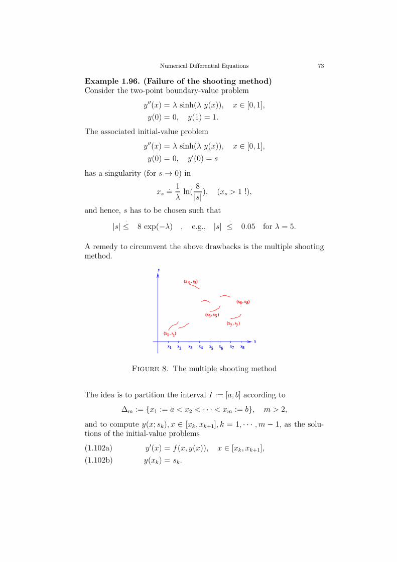
Numerical Differential Equations 73
Example 1.96. (Failure of the shooting method)Consider the two-point boundary-value problem
y′′(x) = λ sinh(λ y(x)), x ∈ [0, 1],
y(0) = 0, y(1) = 1.
The associated initial-value problem
y′′(x) = λ sinh(λ y(x)), x ∈ [0, 1],
y(0) = 0, y′(0) = s
has a singularity (for s→ 0) in
xs.=
1
λln(
8
|s|), (xs > 1 !),
and hence, s has to be chosen such that
|s| ≤·
8 exp(−λ) , e.g., |s| ≤·
0.05 for λ = 5.
A remedy to circumvent the above drawbacks is the multiple shootingmethod.
)5, s5
(x )7, s7
(x
1s,1 )
)3, s3(x
(x
x5x4 6 8x7xx
8), s8
x 3x2x1
(x
y
x
Figure 8. The multiple shooting method
The idea is to partition the interval I := [a, b] according to
∆m := x1 := a < x2 < · · · < xm := b, m > 2,
and to compute y(x; sk), x ∈ [xk, xk+1], k = 1, · · · , m − 1, as the solu-tions of the initial-value problems
y′(x) = f(x, y(x)), x ∈ [xk, xk+1],(1.102a)
y(xk) = sk.(1.102b)

74 Ronald H.W. Hoppe
Here, s1, · · · , sm−1, and sm have to be computed such that the com-posed function
y(x) := y(x; sk), x ∈ [xk, xk+1], 1 ≤ k ≤ m− 1,
y(b) := sm,
is continuous and satisfies the boundary conditions
Fk(sk, sk+1) := y(xk+1; sk)− sk+1 = 0, 1 ≤ k ≤ m− 1,(1.103a)
Fm(s1, sm) := r(s1, sm) = 0.(1.103b)
We note that (1.103a),(1.103b) represents a cyclic system in the n×munknowns sk = (sk,1, · · · , sk,m)T , 1 ≤ k ≤ m. The cyclic system canbe solved by Newton’s method
J(s(ν)) ∆s(ν) = −F (s(ν)), ν ≥ 0,(1.104a)
s(ν+1) = s(ν) +∆s(ν),(1.104b)
where
J(s) = (∂Fk
∂sℓ)m
k,ℓ=1.
The linear system (1.104a) for the Newton increments reads as follows:
G1 −I 0 · · 00 G2 −I ·· · · ·· · · 00 Gm−1 −IA 0 · 0 B
∆s(ν)1
∆s(ν)2
··∆s
(ν)m−1
∆s(ν)m
= −
F (s(1))F (s(2))··F (s(m−1))F (s(m))
where Gk := W (xk+1, xk)|y(x;sk), 1 ≤ k ≤ m − 1, are the Wronski ma-
trices and A := ∂r∂ya, B := ∂r
∂yb.

Numerical Differential Equations 75
1.5.3 Finite difference approximations
Given I := [a, b] ⊂ R and functions f, s ∈ C(I), and r ∈ C1(I),satisfying
0 < c0 ≤ r(x) ≤ c1, x ∈ I , s(x) ≥ 0, x ∈ I,
we consider the two-point boundary value problem
− (r(x) y′(x))′ + s(x) y(x) = f(x), x ∈ [a, b],(1.105a)
y(a) = 0, y(b) = 0.(1.105b)
Introducing the variable
z(x) := r(x) y′(x), x ∈ I,
the second order ordinary differential equation (1.105a) can be writtenas a system of two first order ordinary differential equations
y′(x) = z(x)/r(x), x ∈ I,(1.106a)
z′(x) = s(x) y(x)− f(x), x ∈ I.(1.106b)
We partition the interval I into an equidistant grid
Ih := xk = a + k h | 0 ≤ k ≤ n+ 1
of step size h := (b− a)/(n+ 1) and approximate the derivatives y′(x)and z′(x) in xk+1/2 = xk + h/2, 0 ≤ k ≤ n, by the central differencequotients
1
h(y(xk+1)− y(xk)) ≈
z(xk+1/2)
r(xk+1/2),
1
h(z(xk+1)− z(xk)) ≈ s(xk+1/2) y(xk+1/2)− f(xk+1/2).
Since we want to compute approximations only the grid points xk, 0 ≤k ≤ n+ 1, we replace z(xk+1/2) and y(xk+1/2) by averaging
z(xk+1/2) ≈1
2(z(xk) + z(xk+1)),
y(xk+1/2) ≈1
2(y(xk) + y(xk+1)).
Setting
rk+1/2 := r(xk+1/2) , sk+1/2 := s(xk+1/2) , fk+1/2 := f(xk+1/2),

76 Ronald H.W. Hoppe
the finite difference approximation of (1.105a),(1.105b) amounts to thecomputation of grid functions yh, zh ∈ C(Ih) as the solution of
yh(xk+1) = yh(xk) +h
2 rk+1/2
(zh(xk) + zh(xk+1)),(1.107a)
zh(xk+1) = zh(xk) +h
2(yh(xk) + yh(xk+1)),(1.107b)
yh(a) = yh(b) = 0.(1.107c)
Solving (1.107a) for zh(xk+1) yields
zh(xk+1) = −zh(xk) +2 rk+1/2
h(yh(xk+1)− yh(xk)).(1.108)
The corresponding equation for zh(xk) reads
zh(xk) = −zh(xk−1) +2 rk−1/2
h(yh(xk)− yh(xk−1)).(1.109)
Inserting (1.109) into (1.108) results in
zh(xk+1)− zh(xk−1) = − 2 rk−1/2
h(yh(xk)− yh(xk−1)) +(1.110)
2 rk+1/2
h(yh(xk+1)− yh(xk)).
On the other hand, the addition of (1.107b) for k − 1 and k gives
zh(xk) = zh(xk−1) +h
2sk−1/2 (yh(xk−1) + yh(xk))− h fk−1/2 +
(1.111a)
zh(xk+1) = zh(xk) +h
2sk+1/2 (yh(xk) + yh(xk+1))− h fk+1/2 =⇒
(1.111b)
h
2sk−1/2 yh(xk−1) +
h
2(sk−1/2 + sk+1/2) yh(xk) +
(1.111c)
h
2sk+1/2 yh(xk+1)− (zh(xk+1)− zh(xk−1)) = h fk−1/2 + h fk+1/2.
Inserting (1.110) into yields
(−2 rk−1/2
h+h
2sk−1/2) yh(xk−1) + (
2 rk−1/2
h+
2 rk+1/2
h+h
2sk−1/2) +
(1.112)
h
2sk+1/2 yh(xk) + (−2 rk+1/2
h+h
2sk+1/2) yh(xk+1) = h (fk−1/2 + fk+1/2).

Numerical Differential Equations 77
1.5.4 Galerkin approximations
We multiply (1.105a) with a function ϕ ∈ C10(I) and integrate over I:
−b∫
a
(r(x) y′(x))′ ϕ(x) dx+
b∫
a
s(x) y(x) ϕ(x) dx =
b∫
a
f(x) ϕ(x) dx.
Partial integration of the first integral results in
−b∫
a
(r(x) y′(x))′ϕ(x) dx =
b∫
a
r(x) y′(x)ϕ′(x) dx− (r(x) y′(x)ϕ(x))|ba︸ ︷︷ ︸
= 0
.
Hence, we obtain
b∫
a
r(x) y′(x) ϕ′(x) dx+
b∫
a
s(x) y(x) ϕ(x) dx =
b∫
a
f(x)ϕ(x) dx.
In view of this variational equation, on C10(I) we introduce a norm
according to
‖y‖1 := (
b∫
a
(y′(x)2 + y(x)2) dx )1/2.
The space (C10 (I), ‖ · ‖1 is not complete. We refer to H1
0 (I) as theclosure of (C1
0(I), ‖ · ‖1 with respect to the topology induced by ‖ · ‖1on C1
1(I). Then, the so-called weak formulation of (1.105a),(1.105b)amounts to the computation of y ∈ H1
0 (I) such that for all ϕ ∈ H10 (I)
it holds
b∫
a
r(x) y′(x) ϕ′(x) dx+
b∫
a
s(x) y(x) ϕ(x) dx =
b∫
a
f(x)ϕ(x) dx.
(1.113)
We choose a subspace Sh ⊂ H10 (I) with dim Sh = nh < ∞. Then, the
Galerkin approximation of (1.113) requires the computation of yh ∈ Sh
such that for all ϕh ∈ Sh the finite dimensional variational equation
b∫
a
r(x) y′h(x) ϕ′h(x) dx+
b∫
a
s(x) yh(x) ϕh(x) dx =
b∫
a
f(x)ϕh(x) dx
(1.114)
is satisfied.

78 Ronald H.W. Hoppe
We consider a partition
Ih := xk := a+ k h | 0 ≤ k ≤ n+ 1, h :=b− a
n+ 1,
of I and choose Sh as the linear space S1,0(I; Ih) of linear splines withrespect to Ih:
S1,0(I; Ih) := vh ∈ C0(I) | vh|[xk,xk+1] ∈ P1([xk, xk+1]), 0 ≤ k ≤ n.
The space S1,0(I; Ih) is spanned by the basis functions ϕ(k)h , 1 ≤ k ≤ n,
with
ϕ(k)h (xj) = δjk, 1 ≤ j, k ≤ n.
The solution yh ∈ S1,0(I; Ih) of (1.114) can be written as a linear com-bination of the basis functions according to
yh =n∑
j=1
cj ϕ(j)h .
Then, (1.114) holds true if and only if
n∑
j=1
(b∫
a
r(x) (ϕ(j)h )′(x) (ϕ
(i)h )′(x) dx+
b∫
a
s(x) (ϕ(j)h )(x) (ϕ
(i)h )(x) dx
)
︸ ︷︷ ︸
=: aij
cj
=
b∫
a
f(x) (ϕ(i)h )(x) dx
︸ ︷︷ ︸
=: bi
, 1 ≤ i ≤ n,
i.e., the Galerkin method requires the solution of the linear system
A c = b.(1.115)
Definition 1.97. (Stiffness matrix and load vector)The matrix A = (aij)
ni,j=1 and the vector b = (b1, ..., bn)
T are called thestiffness matrix and the load vector.
Lemma 1.98. (Properties of the stiffness matrix)The stiffness matrix A is a symmetric, positive definite tridiagonalmatrix.

Numerical Differential Equations 79
Lemma 1.99. (Numerical quadrature)If we compute the entries of the stiffness matrix A and of the loadvector b by the quadrature formula
xk+1∫
xk
g(x) dx ≈ h g(xk +h
2) =: h gk+1/2,
we obtain
aii =rk−1/2
h+rk+1/2
h+h
4sk−1/2 +
h
4sk+1/2, 1 ≤ i ≤ n,
ai,i+1 = − rk+1/2
h+h
4sk+1/2, 1 ≤ i ≤ n− 1,
ai−1,i = − rk−1/2
h+h
4sk−1/2, 2 ≤ i ≤ n,
bi =h
2fk−1/2 +
h
2fk+1/2.
Remark 1.100. (Equivalence with finite difference approxima-tion)If the entries of the stiffness matrix and the load vector are computed bynumerical quadrature, the linear system Ac = b coincides with (1.112).

80 Ronald H.W. Hoppe
Literature
U.M. Ascher, R.M.M. Mattheij, and R.D. Russell; Numerical Solu-tion of Boundary Value Problems for Ordinary Differential Equations.SIAM, Philadelphia, 1995
U. Ascher and L.R. Petzold; Computer Methods for Ordinary Differen-tial Equations and Differential-Algebraic Equations. SIAM, Philadel-phia, 1998
K. Atkinson, W. Han, and D. Stewart; Numerical Solution of OrdinaryDifferential Equations. Wiley-Interscience, Hoboken, N.J., 2006
K. E. Brenan , S. L. Campbell and L. R. Petzold; Numerical Solutionof Initial-Value Problems in Differential-Algebraic Equations. SIAM,Philadelphia, 1996
J. Butcher; Numerical Methods for Ordinary Differential Equations.2nd Edition. Wiley, Chichester-New York, 2008
P. Deuflhard and F. Bornemann; Scientific Computing with OrdinaryDifferential Equations. Springer, Berlin-Heidelberg-New York, 2002
C.W. Gear; Numerical Initial Value Problems in Ordinary DifferentialEquations. Prentice-Hall, Englewood Cliffs, NJ., 1971
E. Hairer, S.P. Norsett, and G. Wanner; Solving Ordinary DifferentialEquations I. Nonstiff Problems. 2nd Revised Edition. Springer, Berlin-Heidelberg-New York, 2009
E. Hairer and G. Wanner; Solving Ordinary Differential EquationsII. Stiff and Differential-Algebraic Problems. 2nd Revised Edition.Springer, Berlin-Heidelberg-New York, 2010
E. Hairer, C. Lubich and G. Wanner; Geometric Numerical Integration.Structure-Preserving Algorithms for Ordinary Differential Equations.2nd Edition. Springer, Berlin-Heidelberg-New York, 2010
A. Iserles; A First Course in the Numerical Analysis of DifferentialEquations. Second Edition, Cambridge University Press, Cambridge,2009
P. Kunkel and V. Mehrmann; Differential-Algebraic Equations: Anal-ysis and Numerical Solution. European Mathematical Society, Zurich,2006
L.F. Shampine, I. Gladwell, and S. Thompson; Solving ODEs withMATLAB. Cambridge University Press, Cambridge, 2003
J. Stoer and R. Bulisch; An Introduction to Numerical Analysis. Sec-ond Edition. Springer, Berlin-Heidelberg-New York, 1993

Numerical Differential Equations 81
C. Vuik, F.J. Vermolen, M.B. van Gijzen, and M.J. Vuik; NumericalMethods for Ordinary Differential Equations. Delft Academic Press,Delft, 2014
82 Ronald H.W. Hoppe
2. Partial Differential Equations
2.1 Theoretical foundations and preliminaries
A partial differential equation is an equation which contains an un-known function in several independent variables along with certainpartial derivatives of that function. The order of the differential equa-tion corresponds to the highest partial derivative that occurs in theequation.
Let Ω be a domain in Rd, d ∈ N, d ≥ 2, and let α be a multi-index inNd
0,N0. For a function u ∈ Cm(Ω), m ∈ N, we denote by Dαu(x), |α| :=∑d
i=1 αi ≤ m, the partial derivative
Dαu(x) :=∂|α|u(x)
∂xα11 · · ·∂xαd
d
.
Definition 2.1. (Partial differential equation of m-th order)Let F : Ω× RN → R, N := cardα ∈ Nd
0| | |α| ≤ m, and u ∈ Cm(Ω).Then
F (x, (Dαu(x))|α|≤m) = 0, x ∈ Ω(2.1)
is called a nonlinear partial differential equation of order m.A partial differential equation (2.1) is called quasilinear, if it is linear inthe highest partial derivatives Dαu, |α| = m, i.e., if there exist functionsaα : Ω×RN1 → R and F1 : Ω×RN1 → R, N1 ∈ N, such that the functionF in (2.1) has the representation
F (x, (Dαu(x))|α|≤m) =(2.2)∑
|α|=m
aα(x, (Dβu(x))|β|≤m−1)D
αu(x) + F1(x, (Dβu(x))|β|≤m−1).
A quasilinear partial differential equation is said to be semilinear, ifthe coefficient function aα, |α| = m, only depends on xi, 1 ≤ i ≤ d, butneither on u not its partial derivatives.A partial differential equation is called linear, if the function F in (2.1)is linear in u and its partial derivatives Dαu, |α| ≤ m, i.e., if there existfunctions aα : Rd → R, |α| ≤ m, and f : Rd → R such that
Lu := L(·, D)u = f in Ω ⊂ Rd,(2.3)

Numerical Differential Equations 83
where L(·, D) denotes the linear partial differential operator
L(x,D)u :=∑
|α|≤m
aα(·) Dα.(2.4)
The differential operator
LH(·, D)u :=∑
|α|=m
aα(·) Dα(2.5)
is called the main part of L(·, D).
The classification of linear partial differential equations ofm-th orderis done by means of the symbol.
Definition 2.2. (Symbol)The symbol of the linear partial differential operator (2.4) is given by
L(x, iξ) :=∑
|α|≤m
aα(x)(iξ)α , ξα :=
d∏
ν=1
ξανν ,(2.6)
where i stands for the imaginary unit. We refer to
LH(x, iξ) :=∑
|α|=m
aα(x)(iξ)α(2.7)
as the main part of the symbol.
In the sequel we will restrict ourselves to the case m = 2. Givencontinuous functions aij : Rd → R, 1 ≤ i, j ≤ d, and bi : R
d → R, aswell as c : Rd → R, a linear partial differential equation of second ordercan be written in the form
Lu =
d∑
i,j=1
aij uxixj+
d∑
i=1
bi uxi+ c u = f,(2.8)
where uxi:= ∂u/∂xi and uxixj
:= ∂2u/∂xi∂xj . The main part LH(x, iξ)of the symbol L(x, iξ) is given by
LH(x, iξ) = −d∑
i,j=1
aij(x) ξiξj.(2.9)
We define A(x) ∈ Rd×d as the matrix
(2.10) A(x) := (−aij(x))di,j=1.
Hence, the main part LH(x, iξ) satisfies
LH(x, iξ) = ξTA(x)ξ

84 Ronald H.W. Hoppe
and thus represents a quadratic form in ξ.
Definition 2.3. (Classification of linear second order partialdifferential equations)A linear second order partial differential equation (2.8) is called ellipticin x ∈ Ω, if all eigenvalues of the matrix A(x) have the same sign. Itis said to be parabolic in x ∈ Ω, if A(x) is singular. Finally, it is calledhyperbolic in x ∈ Ω, if all but one eigenvalue of A(x) have the samesign and one eigenvalue has the opposite sign. Note that eigenvaluesare counted according to their multiplicity.A linear second order partial differential equation (2.8) is called elliptic(parabolic, hyperbolic) in Ω, if it is elliptic (parabolic, hyperbolic) forall x ∈ Ω.
The main part of linear second order partial differential equations ofthe same type can be transformed by a principal axis transformationto a canonical form.
Example 2.4. (Poisson and Laplace equation)The canonical form of an elliptic second order differential equation isthe Poisson equation
−∆u = f(2.11)
with the Laplace operator
∆ :=d∑
i=1
∂2
∂x2i.(2.12)
In case f ≡ 0 (2.11) is said to be the Laplace equation. The symbol of
−∆ is∑d
i=1 ξ2i . Hence, A = A(x) has the d-fold eigenvalue +1.
Example 2.5. (Heat equation)The canonical form of a linear second order parabolic equation is theheat equation
ux1 −d∑
i=2
uxixi= f(2.13)
with the symbol iξ1 +∑d
i=2 ξ2i . Here, A = A(x) has the simple eigen-
value 0 and the (d− 1)-fold eigenvalue +1.The heat equation represents the temporal and spatial temperaturedistribution of a heat conducting material.
Numerical Differential Equations 85
Example 2.6. (Wave equation)The canonical form of a linear second order hyperbolic differential equa-tion is the wave equation
ux1x1 −d∑
i=2
uxixi= f.(2.14)
The symbol is −ξ21 +∑d
i=2 ξ2i . The matrix A = A(x) has the simple
eigenvalue −1 and the (d− 1)-fold eigenvalue +1.The wave equation describes the temporal and spatial propagation ofacoustic waves.
Example 2.7. (Tricomi equation)In general, partial differential equations may change its type within adomain. An example is the Tricomi equation
x2 ux1x1 + ux2x2 = 0.(2.15)
The symbol is −x2ξ21 − ξ22 . Hence, the Tricomi equation is elliptic forx2 > 0, parabolic for x2 = 0, and hyperbolic for x2 < 0.
The classification of linear second order partial differential equations isclosely related to the notion of characteristics.
Definition 2.8. (Characteristics)Let φ be continuously differentiable in Rd. Then, the (d−1)-dimensionalmanifold
C := x ∈ Rd | φ(x) = 0
is said to be characteristic in x∗ ∈ Rd, if it holds
φ(x∗) = 0 and (∇φ(x∗))TA(x∗)∇φ(x∗) = 0.(2.16)
The manifold C is called a characteristics, if it is characteristic in eachof its points.
It follows from Definition 2.8 that elliptic partial differential equationsdo not possess real characteristics. For d = 2 the characteristics of theheat equation (2.13) are the straight lines x2 = const. parallel to thex1-Achse, whereas the characteristics of the wave equation (2.14) arethe straight lines x2 ± x1 = const..
A classical existence and uniqueness result is the Theorem of Cauchy-Kovalevskaya for real analytic solutions of the so-called Cauchy prob-lem. We consider the following system of quasilinear partial differential

86 Ronald H.W. Hoppe
equations of first order
(ui)xd=
k∑
j=1
∑
|α|≤1
a(ij)α (x′,u)Dαuj, 1 ≤ i ≤ k,(2.17)
where x′ := (x1, · · · , xd−1)T and u := (u1, · · · , uk)T .
Definition 2.9. (Real analytic solution)A function g : Rd → R is called a real analytic function in x∗ ∈ Rd,if there exists a neighborhood U(x∗) such that for all x ∈ U(x∗) thefunction g can be written as a Taylor series
g(x) =∑
α∈Nd0
cα(x− x∗)α.
The function is said to be real analytic in Rd, if it is real analytic ineach point x∗ ∈ Rd.
If the coefficient functions a(ij)α , |α| ≤ 1, 1 ≤ i, j ≤ k, are real analytic in
the origin p0 of Rd+k−1, the vector-valued function u = (u1, · · · , uk)Twith ui : R
d → R, 1 ≤ i ≤ k, is called a real analytic solution of (2.17),if the functions ui, 1 ≤ i ≤ k, are real analytic in p0 and if (2.17) issatisfied in p0.
If the functions a(ij)α are real analytic in Rd, the function u is said to be
a real analytic solution of (2.17) in Rd, if the functions ui, 1 ≤ i ≤ k,are real analytic in Rd and if (2.17) is satisfied in each point x∗ ∈ Rd.
The Cauchy problem associated with (2.17) is to find a locally uniquesolution for given initial conditions on the (d − 1)-dimensional hyper-plane
H := x ∈ Rd | xd = 0,(2.18)
which is not a characteristics of (2.17).
Definition 2.10. (Cauchy problem)Let H be given by (2.18) and assume that gi : H → R, 1 ≤ i ≤ k,are given functions. The Cauchy problem associated with (2.17) is tocompute a vector-valued function u = (u1, · · · , uk)T such that (2.17)and
ui(x) = gi(x), x ∈ H, 1 ≤ i ≤ k,(2.19)
hold true.

Numerical Differential Equations 87
The Theorem of Cauchy-Kovalevskaya provides conditions for the lo-cal existence and uniqueness of a real analytic solution of the Cauchyproblem.
Theorem 2.11. (Theorem of Cauchy-Kovalevskaya)
Suppose that the functions a(ij)α , |α| ≤ 1, 1 ≤ i, j ≤ k, are real analytic
in the origin of Rd+k−1 and that the functions gi, 1 ≤ i ≤ k, are realanalytic in the origin of the hyperplane H. Then the Cauchy problemadmits a locally unique real analytic solution.
Proof. The proof relies on the technique of real analytic majorants. Fordetails we refer to Renardy and Rogers.

88 Ronald H.W. Hoppe
2.2 Linear second order elliptic boundary value problems
2.2.1 Preliminaries
We consider linear second order elliptic differential equations in a boundeddomain Ω ⊂ Rd
Lu := −d∑
i,j=1
aij∂2u
∂xi∂xj+
d∑
i=1
bi∂u
∂xi+ cu = f(2.20)
under the following assumptions on the coefficient functions
It holds aij, bi, c ∈ C(Ω), 1 ≤ i, j ≤ d, and there exists a(2.21a)
constant C > 0, such that for all 1 ≤ i, j ≤ d and x ∈ Ω
|aij(x)| , |bi(x)| , |c(x)| ≤ C ,
The functions aij are symmetric, i.e., for all(2.21b)
1 ≤ i, j ≤ d and x ∈ Ω it holds
aij(x) = aji(x) ,
and the matrix-valued function (aij)di,j=1 is uniformly
positive definite in Ω , i.e., there exists a constant α > 0 ,
such that for all x ∈ Ω and ξ ∈ Rd
d∑
i,j=1
aij(x)ξiξj ≥ α |ξ|2 .
For the sake of uniqueness of a solution of (2.20) we need boundaryconditions on the boundary Γ = ∂Ω.
Definition 2.12. (Dirichlet, Neumann, and Robin problem)Under the assumptions (2.21a),(2.21b) let L be the linear second orderdifferential operator given by (2.20) and suppose further that f ∈ C(Ω)and uD ∈ C(Γ). Then, the boundary-value problem
Lu(x) = f(x), x ∈ Ω,(2.22a)
u(x) = uD(x), x ∈ Γ,(2.22b)
is called an inhomogeneous Dirichlet problem. If uD ≡ 0, it is said tobe a homogeneous Dirichlet problem. A function u ∈ C2(Ω) ∩ C(Ω) iscalled a classical solution, if u pointwise satisfies (2.22a),(2.22b).In case of boundary conditions of the form
(ν · ∇u)(x) = uN(x), x ∈ Γ,(2.23)

Numerical Differential Equations 89
where ν is the exterior unit normal on Γ and uN ∈ C(Γ), the boundary-value problem is referred to as a Neumann problem.Boundary conditions of the form
(ν · ∇u)(x) + d(x)u(x) = uR(x), x ∈ Γ,(2.24)
where d, uR ∈ C(Γ), are called Robin boundary conditions.It is of course possible to prescribe different boundary conditions ondifferent parts of the boundary.
If c(x) ≥ 0, x ∈ Ω, in (2.20), the uniqueness of a solution of the Dirichletproblem (2.22a),(2.22b) follows from the maximum principle of Hopf.
Theorem 2.13. (Maximum principle of Hopf)In addition the assumptions (2.21a),(2.21b) suppose that c(x) ≥ 0, x ∈Ω, and that the function u ∈ C2(Ω) satisfies the inequality
Lu(x) ≤ 0, x ∈ Ω.(2.25)
If there exists a point x0 ∈ Ω such that
u(x0) = supx∈Ω
u(x) ≥ 0,(2.26)
then it holds
u(x) = const., x ∈ Ω.(2.27)
Proof. We refer to Jost.
Corollary 2.14. (Uniqueness of the Dirichlet problem)Under the assumptions of Theorem 2.13 the Dirichlet problem (2.22a),(2.22b) admits a unique classical solution.
Proof. Let u1, u2 be two classical solutions and z := u1 − u2. ThenLz(x) = 0, x ∈ Ω, and Theorem 2.13 implies z(x) = const., x ∈ Ω.Since z(x) = 0, x ∈ Γ, it follows that z ≡ 0.
For the Poisson equation (2.11) the existence of a solution of the Dirich-let problem can be shown by means of Green’s representation formula.We assume Ω to be a domain whose boundary Γ admits a parametriza-tion by a C1 function (C1-domain).

90 Ronald H.W. Hoppe
Theorem 2.15. (First and second Green’s formula)Let Ω ⊂ Rd be a C1-domain and assume that u, v ∈ C2(Ω). Then, theequation
∫
Ω
∆u v dx+
∫
Ω
∇u · ∇v dx =
∫
Γ
ν · ∇u v dσ(2.28)
is called Green’s first formula, whereas the equation∫
Ω
(
∆u v − u ∆v)
dx =
∫
Γ
(
ν · ∇u v − u ν · ∇v)
dσ(2.29)
is referred to as Green’s second formula.
Proof. The proof of (2.28) follows from the Gauss’ theorem∫
Ω
∇ · q dx =
∫
Γ
ν · q dσ
applied to the vector-valued function q := v∇u. Exchanging u and vin (2.28) and subtracting the resulting equation from (2.28) results in(2.29).
Definition 2.16. (Fundamental solution)A function u ∈ C2(Ω) is called a harmonic function in Ω, if u satisfiesthe Laplace equation, i.e., ∆u(x) = 0, x ∈ Ω.The function
Γ(x, y) :=
12π
ln(|x− y|) , d = 21
d(2−d)|Bd1 |
|x− y|2−d , d > 2 , x, y ∈ Rd, x 6= y,(2.30)
where |Bd1 | is the volume of the unit ball in Rd, is called the fundamental
solution of the Laplace equation. As a function of x it is a harmonicfunction in Rd \ y.The notion ’fundamental solution’ is justified by Green’s representationformula.
Theorem 2.17. (Green’s representation formula)Assume that Ω ⊂ Rd is a C1-domain and Γ(·, ·) the fundamental solu-tion given by (2.30). Then, for u ∈ C2(Ω) and y ∈ Ω it holds
u(y) =
∫
Ω
Γ(x, y) ∆u(x) dx +(2.31)
∫
∂Ω
(
u(x) ν · ∇xΓ(x, y)− Γ(x, y) ν · ∇u(x))
dσ(x),

Numerical Differential Equations 91
where ∇x stands for the gradient with respect to the differentiation inx.
Proof. The proof can be done by means of Green’s second formula(2.29). For details we refer to Jost.
Definition 2.18. (Green’s function)A function G(x, y), x, y ∈ Ω, x 6= y, is called Green’s function, if thefollowing two conditions are satisfied:
G(x, y) = 0, x ∈ ∂Ω,(2.32a)
The function G(x, y)− Γ(x, y) is harmonic in x ∈ Ω.(2.32b)
Green’s function enables an explicit representation of the solution ofthe inhomogeneous Dirichlet problem for the Poisson equation (2.11).
Theorem 2.19. (Solution of the inhomogeneous Dirichlet prob-lem)Under the assumptions of Theorem 2.17 let G(x, y) be a Green’s func-tion for Ω. Then, the following statements hold true:
(i) If u ∈ C2(Ω)∩C(Ω) is the classical solution of the inhomogeneousDirichlet problem for the Poisson equation (2.11), for y ∈ Ω we have
u(y) =
∫
Ω
G(x, y) f(x) dx+
∫
∂Ω
uD(x) ν · ∇xG(x, y) dσ(x).(2.33)
(ii) If f is a Holder continuous function in Ω and uD ∈ C(∂Ω), thenthe function u given by (2.33) is the classical solution of the inhomo-geneous Dirichlet problem for the Poisson equation.
Proof. The proof of (i) follows by the application of Green’s secondformula (2.29) to the function v(x) = G(x, y) − Γ(x, y). The proofof (ii) requires further results on the regularity of solutions of ellipticpartial differential equations. We refer to Jost.

92 Ronald H.W. Hoppe
2.2.2 Finite difference approximations
We consider the numerical solution of Poisson’s equation (2.11) withinhomogeneous Dirichlet boundary conditions by a finite differencemethod based on the approximation of the partial derivatives by dif-ference quotients. To this end we assume Ω to be a d-dimensionalcube.
Definition 2.20. (Grid point set)Let Ω := (a, b)d with a, b ∈ R, a < b, and h := (b− a)/(N + 1), N ∈ N.Then the set
Ωh := (xi1 , · · · , xid)T | xij = a+ ijh , 0 ≤ ij ≤ N + 1 , 1 ≤ j ≤ dis called a grid point set with step size h. The elements of Ωh arecalled grid points. The set Ωh is a particular example of a uniform orequidistant grid where the grid points have the same distance to eachother.We further refer to Ωh := Ωh ∩ Ω as the set of interior grid points andto Γh := Ωh \ Ωh as the set of boundary grid points.
For the approximation of the partial derivatives ∂u/∂xi, ∂2u/∂x2i , 1 ≤
i ≤ d, we consider the following difference quotients:
Definition 2.21. (Difference quotients)Let u : Ω → R and let ei, 1 ≤ i ≤ d, be the i-th unit vector in Rd.Then the difference quotients
D+h,iu(x) := h−1(u(x+ hei)− u(x)),
D−h,iu(x) := h−1(u(x)− u(x− hei)),
D1h,iu(x) := (2h)−1(u(x+ hei)− u(x− hei))
are called the forward, the backward, and the central difference quo-tients for the first partial derivatives ∂u/∂xi, 1 ≤ i ≤ d.The difference quotients
D2h,i,iu(x) := h−2(u(x+ hei)− 2u(x) + u(xi − hei))
are called the central difference quotients for the second partial deriva-tives ∂2u/∂x2i , 1 ≤ i ≤ d.
It follows from Taylor expansion that for u ∈ C2(Ω) the difference quo-tients D±
h,iu provide an approximation of ∂u/∂xi of order O(h), whereas
for u ∈ C4(Ω) the central difference quotients D1h,iu bzw. D2
h,iu give
rise to approximations of ∂2u/∂x2i of order O(h2).

Numerical Differential Equations 93
As far as approximations of the mixed second partial derivatives∂2u/∂xi∂xj , i 6= j, are concerned, we refer to Strikwerda.A convenient tool to characterize difference quotients are differencestars (cf. Figure 9). Here, the grid points marked by • are those gridpoints involved in the difference quotient. The number next to • refersto the weight, i.e., the factor of the function value times h−2 in thatgrid point.
1
1
−4 1
1
Figure 9. Difference star for the Laplacian ∆ (d = 2)
Definition 2.22. (Discrete Laplace operator)The difference operator
∆h :=
d∑
i=1
D2h,i,i
is called the discrete Laplace operator. For u ∈ C4(Ω) the discreteLaplace operator ∆hu is an approximation of ∆u of order O(h2).In case d = 2 the associated difference star is displayed in Figure 9.Since five grid points are involved, it is also referred to as the five-pointapproximation of the Laplacian.
For a bounded domain Ω ⊂ Rd with a curved boundary Γ the definitionof interior grid points and boundary grid points has to be made moreprecise.
Definition 2.23. (Domain with curved boundary)Let Ω ⊂ Rd be a bounded connected domain with boundary Γ and letR
dh be the uniform grid point set
Rdh := x = (x1, · · · , xd)T | xi = ih , i ∈ Z.
Then Ωh := Rdh ∩ Ω is called the set of interior grid points. A point
x ∈ Γ is called a boundary grid point, if there exists an interior grid
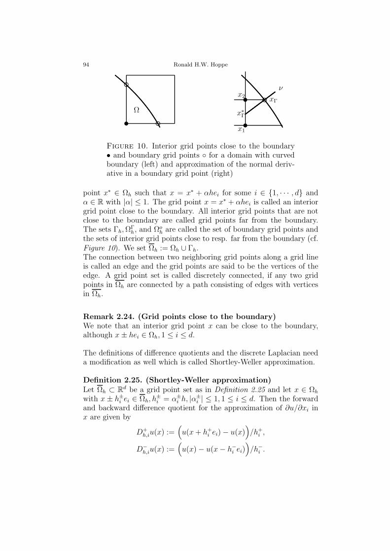
94 Ronald H.W. Hoppe
Ω
xΓ
ν
x∗Γ
x1
x2
Figure 10. Interior grid points close to the boundary• and boundary grid points for a domain with curvedboundary (left) and approximation of the normal deriv-ative in a boundary grid point (right)
point x∗ ∈ Ωh such that x = x∗ + αhei for some i ∈ 1, · · · , d andα ∈ R with |α| ≤ 1. The grid point x = x∗ + αhei is called an interiorgrid point close to the boundary. All interior grid points that are notclose to the boundary are called grid points far from the boundary.The sets Γh,Ω
Γh , and Ωo
h are called the set of boundary grid points andthe sets of interior grid points close to resp. far from the boundary (cf.Figure 10). We set Ωh := Ωh ∪ Γh.The connection between two neighboring grid points along a grid lineis called an edge and the grid points are said to be the vertices of theedge. A grid point set is called discretely connected, if any two gridpoints in Ωh are connected by a path consisting of edges with verticesin Ωh.
Remark 2.24. (Grid points close to the boundary)We note that an interior grid point x can be close to the boundary,although x± hei ∈ Ωh, 1 ≤ i ≤ d.
The definitions of difference quotients and the discrete Laplacian needa modification as well which is called Shortley-Weller approximation.
Definition 2.25. (Shortley-Weller approximation)Let Ωh ⊂ R
d be a grid point set as in Definition 2.25 and let x ∈ Ωh
with x ± h±i ei ∈ Ωh, h±i = α±
i h, |α±i | ≤ 1, 1 ≤ i ≤ d. Then the forward
and backward difference quotient for the approximation of ∂u/∂xi inx are given by
D+h,iu(x) :=
(
u(x+ h+i ei)− u(x))
/h+i ,
D−h,iu(x) :=
(
u(x)− u(x− h−i ei))
/h−i .
Numerical Differential Equations 95
The central difference quotient for the second partial derivatives∂2u/∂x2i is given by
D2h,i,iu(x) :=
2
h+i + h−i
(u(x+ h+i ei)− u(x)
h+i+u(x− h−i ei)− u(x)
h−i
)
.
For d = 2 and x = (x1, x2) ∈ Ωh with (x1 ± α±1 h, x2 ± α±
2 h) ∈ Ωh, thediscrete Laplacian ∆h has the representation
∆hu(x) :=2
h2
( 1
α+
1 (α+
1 + α−
1 )u(x1 + α+
1h, x2) +
1
α−
1 (α+
1 + α−
1 )u(x1 − α−
1h, x2)+
(2.34)
1
α+
2 (α+
2 + α−
2 )u(x1, x2 + α+
2 h, ) +1
α−
2 (α+
1 + α−
2 )u(x1, x2 − α−
2 h)−(2.35)
(1
α+
1 α−
1
+1
α+
2 α−
2
)u(x1, x2))
.(2.36)
Remark 2.26. (Miscellaneous)(i) In grid points close to the boundary, the central difference quotientfor the second partial derivatives and the discrete Laplacian are ingeneral only approximations of order O(h).(ii) The definition of the difference quotients and the definition ofthe discrete Laplacian can be generalized to non-equidistant grids. Werefer to Strikwerda.
Definition 2.27. (Shortley-Weller approximation of the normalderivative)Let ν · ∇u be the normal derivative in xΓ ∈ Γh, where ν stands forthe outward normal unit vector in xΓ, and let x∗Γ ∈ Ωh be the firstintersection of the normal through xΓ with a grid line (see Figure 10(right)). Further, let xi, 1 ≤ i ≤ 2, be those grid points on that grid lineclose to x∗Γ, where we suppose that the grid is sufficiently fine to ensurexi ∈ Ωh, 1 ≤ i ≤ 2. We refer to u(x∗Γ) as the linearly interpolated valuewith respect to u(x1) and u(x2). Then
(2.37) Dνhu(xΓ) :=
u(xΓ)− u(x∗Γ)
|xΓ − x∗Γ|is an approximation of the normal derivative in xΓ.
Definition 2.28. (Grid function)Let Ωh be a grid point set as in Definition 2.25. A function uh : Ωh → R
is called a grid function. We refer to C(Ωh) as the normed linear space

96 Ronald H.W. Hoppe
of grid functions equipped with the discrete analogue of the maximumnorm
‖uh‖h := maxx∈Ωh
|uh(x)|.(2.38)
We consider a difference approximation of Poisson’s equation (2.11)with inhomogeneous Dirichlet boundary conditions based on the useof the discrete Laplacian. Given grid functions fh ∈ C(Ωh) and u
Dh ∈
C(Γh), we are looking for a grid function uh ∈ C(Ωh) such that
−∆huh = fh in Ωh,(2.39a)
uh = uDh on Γh.(2.39b)
The existence and uniqueness of a solution can be shown either bymeans of a discrete Green’s function and a discrete maximum principleor by the study of the resulting linear algebraic system. Here, wechoose the latter approach and restrict ourselves to the case d = 2and Ω = (a, b)2 as well as a uniform grid Ωh. The unknown values ofthe grid function uh the interior grid points x ∈ Ωh can be interpretedas the components of a vector. The structure of the associated linearalgebraic system depends on the ordering of the grid points.
Definition 2.29. (Lexicographic ordering of grid points)Let Ω = (a, b)2, a, b ∈ R, a < b, and let Ωh be a uniform grid of stepsize h := (b − a)/(N + 1), N ∈ N, with the interior grid points x =(xi, xj)
T , 1 ≤ i, j ≤ N, where xi = a+ ih. The ordering of the interiorgrid points from bottom to top and from left to right according to
x(i−1)N+j = (a + ih, a+ jh)T , 1 ≤ i, j ≤ N,
is called the lexicographic ordering.The ordering such that grid points with even i + j are counted firstfollowed by those with odd i+j is said to be the checkerboard ordering.
For an ordering of the interior grid points according to Definition 2.29,the values of the grid function in the interior grid points can be iden-tified with a vector with nh := N2 components. For ease of notationwe choose the same symbol as for the grid function, i.e., we defineuh ∈ Rnh by means of uh,i := uh(xi), 1 ≤ i ≤ nh. Then (2.39a),(2.39a)is equivalent with a linear algebraic system
Ahuh = bh(2.40)

Numerical Differential Equations 97
with a coefficient matrix Ah ∈ Rnh×nh and a vector bh ∈ Rnh, whosecomponents are given by the values of fh and uDh .In case of a lexicographic ordering, Ah is a block tridiagonal matrix
Ah = h−2 tridiag(−I, T,−I),(2.41)
where the diagonal blocks T ∈ RN×N are tridiagonal matrices of theform
T = tridiag(−1, 4,−1)(2.42)
and the sub- and super-diagonal blocks are the negative N × N unitmatrix.The matrix Ah is a symmetric, positive definite matrix with the eigen-values
λij(Ah) = 4h−2(
sin2(iπh/2) + sin2(jπh/2))
, 1 ≤ i, j ≤ N,(2.43)
and the associated orthonormal eigenvectors x(ij) ∈ Rnh, 1 ≤ i, j ≤ N,with the components
x(ij)kℓ =
h
2sin(ihkπ) sin(jhℓπ), 1 ≤ k, ℓ ≤ N.
The properties of Ah imply the unique solvability of the linear alge-braic system (2.40) and hence the unique solvability of the differenceapproximation (2.39a),(2.39b). They also imply the convergence of uhto the solution u, provided that fh → f and uDh → uD as h→ 0.
Definition 2.30. (Convergence of finite difference approxima-tions)For Ω := (a, b)2, a, b ∈ R, a < b, and a uniform grid Ωh with step sizeh > 0 let u : Ω → R be the classical solution of Poisson’s equa-tion (2.11) with inhomogeneous Dirichlet boundary conditions andlet uh ∈ C(Ωh) be the solution of its finite difference approximation(2.39a),(2.39b). The grid function eh(x) = u(x) − uh(x), x ∈ Ωh, iscalled the global discretization error. The finite difference approxima-tion (2.39a),(2.39b) is said to converge, if
‖eh‖h → 0 as h→ 0.
It is said to be convergent of order p, if there exists a constant C > 0,independent of h, such that for sufficiently small h it holds
‖eh‖h ≤ C hp.
Sufficient conditions for the convergence are the consistency of the fi-nite difference approximation with the boundary value problem andthe stability of the finite difference approximation. The consistency is
98 Ronald H.W. Hoppe
measured by means of the local discretization error which results, ifthe solution u of the boundary value problem is inserted into the finitedifference approximation.
Definition 2.31. (Consistency and order of consistency)Let u be the classical solution of the boundary value problem and let fhand uDh be the grid functions in (2.39a),(2.39b). Then the grid functionτh ∈ C(Ωh) given by
τh(x) :=
−∆hu(x)− fh(x) , x ∈ Ωh
u(x)− uDh (x) , x ∈ Γh
is called the local discretization error. The finite difference approxima-tion (2.39a),(2.39b) is said to be consistent with the boundary valueproblem, if
‖τh‖h → 0 as h→ 0.
It is said to be consistent of order p, if there exists a constant C > 0,independent of h, such that for sufficiently small h it holds
‖τh‖h ≤ C hp.
Lemma 2.32. (Order of consistency for the finite differenceapproximation of Poisson’s equation)Assume that the solution u of Poisson’s equation (2.11) with inhomo-geneous Dirichlet boundary conditions satisfies u ∈ C4(Ω) and that
maxx∈Ωh
|f(x)− fh(x)| = O(h2) , maxx∈Γh
|uD(x)− uDh (x)| = O(h2).
Then the finite difference approximation (2.39a),(2.39b) is consistentwith Poisson’s equation (2.11) with inhomogeneous Dirichlet boundaryconditions of order p = 2.
Proof. Under the assumptions on fh and uDh the proof follows from theapproximation property of the discrete Laplacian.
Remark 2.33. (General bounded domains)The result of Lemma 2.32 can be easily generalized to boundary valueproblems in higher dimensions.For general bounded domains and the use of the Shortley-Weller ap-proximation, in general the order of consistency is reduced to p = 1.
Numerical Differential Equations 99
2.2.3 Sobolev spaces
We give a brief survey on Sobolev spaces and its associated dual spacesand trace spaces. For details we refer to Adams and Tartar.
Let Ω be a bounded domain in Rd. We denote by Ω the closure andby Γ = ∂Ω := Ω \ Ω the boundary of Ω. Moreover, let Ωe := Rd \ Ωthe associated exterior domain.We define Cm(Ω), m ∈ N0, as the linear space of all continuous func-tions in Ω with continuous partial derivatives Dαu, |α| ≤ m,. We notethat Cm(Ω) is a Banach space with respect to the norm
‖u‖Cm(Ω) := max0≤|α|≤m
supx∈Ω
|Dαu(x)|.
Further, we define Cm,α(Ω), m ∈ N0, 0 < α < 1, as the linear spaceof all functions in Cm(Ω) whose m-th partial derivatives are Holdercontinuous, i.e., for all β ∈ Nd
0 with |β| = m there exist constantsΓβ > 0 such that for all x, y ∈ Ω it holds
|Dβu(x)−Dβu(y)| ≤ Γβ |x− y|α.Cm,α(Ω) is a Banach space with respect to the norm
‖u‖Cm,α(Ω) := ‖u‖Cm(Ω) + max|β|=m
supx,y∈Ω
|Dβu(x)−Dβu(y)||x− y|α .
We refer to Cm0 (Ω) as the subspace of Cm(Ω) of all functions with com-
pact support in Ω. Moreover, C∞(Ω) stands for the linear space of allarbitrarily often continuously differentiable functions and C∞
0 (Ω) is thesubspace of C∞(Ω) of all functions with compact support in Ω.In the sequel, we restrict ourselves to Lipschitz-domains which are de-fined as follows:
Definition 2.34. (Lipschitz domain)A bounded domain Ω ⊂ Rd with boundary Γ is called a Lipschitzdomain, if there exist constants α > 0, β > 0, and a finite numberof local coordinate systems (xr1, x
r2, ..., x
rd), 1 ≤ r ≤ R, as well as local
Lipschitz-continuous mappings
ar : xr = (xr2, ..., xrd) ∈ R
d−1 | |xri | ≤ α , 2 ≤ i ≤ d → R
such that
Γ =
R⋃
r=1
(xr1, xr) | xr1 = ar(xr) , |xr| < α,
(xr1, xr) | ar(xr) < xr1 < ar(xr) + β , |xr| < α ⊂ Ω , 1 ≤ r ≤ R,
(xr1, xr) | ar(xr)− β < xr1 < ar(xr) , |xr| < α ⊂ Ωe , 1 ≤ r ≤ R.

100 Ronald H.W. Hoppe
The geometric interpretation of the conditions in Definition 2.34 is thatboth Ω and the exterior domain Ωe are located on exactly one side ofthe boundary Γ.
If the mappings in Definition 2.34 are smoother, the domains are calledCm-domains of Cm,α-domains, m ∈ N.
Definition 2.35. (Cm-domain and Cm,α-domain)A Lipschitz domain Ω ⊂ Rd is said to be a Cm-domain (Cm,α-domain),if the functions ar, 1 ≤ r ≤ R, in Definition 2.34 are Cm-functions(Cm,α-functions).
We denote by L2(Ω) the linear space of Lebesgue square integrableFunctions in Ω. We note that L2(Ω) is a Hilbert space with respect tothe inner product
(v, w)0,Ω :=
∫
Ω
vw dx.
The associated norm will be denoted by ‖ · ‖0,Ω.Sobolev spaces are based on the concept of weak (distributional) deriva-tives:
Definition 2.36. (Weak derivative)Let u ∈ L2(Ω) and α ∈ Nd
0. The function u is said to be differentiablein the weak sense, if there exists a function v ∈ L2(Ω) such that
∫
Ω
uDαϕ dx = (−1)|α|∫
Ω
vϕ dx , ϕ ∈ C∞0 (Ω).
We set Dαwu := v and refer to Dα
wu as the weak (distributional) deriv-ative of u.
Example 2.37. (Weak derivative)Let d = 1 and Ω := (−1,+1). The function u(x) := |x|, x ∈ Ω, is notdifferentiable in the origin. However, it has a weak derivative D1
wu,given by
D1wu =
−1 , x < 0+1 , x > 0
.

Numerical Differential Equations 101
For ϕ ∈ C∞0 (Ω) partial integration yields
+1∫
−1
u(x)D1ϕ(x) dx =
0∫
−1
u(x)D1ϕ(x) dx+
+1∫
0
u(x)D1ϕ(x) dx =
= −0∫
−1
D1wu(x)ϕ(x) dx+ (uϕ)|0−1 −
+1∫
0
D1wu(x)ϕ(x) dx+ (uϕ)|10 =
=
+1∫
−1
D1wu(x)ϕ(x) dx − [u(0)]ϕ(0),
where [u(0)] := u(0+)− u(0−) denotes the jump of u in x = 0. Sinceu is continuous, it follows that [u(0)] = 0 which allows to conclude.
Definition 2.38. (Sobolev space)Let m ∈ N0. The linear space
Wm(Ω) := u ∈ L2(Ω) | Dαwu ∈ L2(Ω), |α| ≤ m(2.44)
is called a Sobolev space. It is a Hilbert space with respect to the innerproduct
(u, v)m,Ω :=∑
|α|≤m
∫
Ω
DαwuD
αwv dx.(2.45)
The associated norm will be denoted by ‖ · ‖m,Ω. We further refer to| · |m,Ω as the seminorm
|u|m,Ω :=( ∑
|α|=m
∫
Ω
(Dαu )
2 dx)1/2
.(2.46)
A natural question is whether Cm(Ω) is dense in Wm(Ω). To this endwe consider the linear space
Cm,∗(Ω) := u ∈ Cm(Ω) | ‖u‖m,p,Ω <∞,which is a normed linear space with respect to the norm ‖ · ‖m,Ω, butnot complete. We denote by Hm(Ω) its completion with respect to the‖ · ‖m,Ω-norm
Hm(Ω) := Cm,∗(Ω)‖·‖m,Ω
.(2.47)
A famous result by Meyers and Serrin says that the spaces Wm(Ω) andHm(Ω) coincide.
We define Hm0 (Ω), m ∈ N, as the completion of (Cm
0 (Ω), ‖ · ‖m,Ω).

102 Ronald H.W. Hoppe
Definition 2.39. (Sobolev spaces with negative integer indices)
Let Ω ⊂ Rd be a bounded Lipschitz domain and let m be a negative
integer. Then the Sobolev space Wm(Ω) is defined as the dual spaceof W−m(Ω).
Definition 2.40. (Sobolev spaces with broken indices)For Ω = Rd we define the Sobolev space Hs(Rd) with broken indexs ∈ R+ by means of the Fourier transform v of a function v ∈ C∞
0 (Rd)
v(ξ) := (1
2π)d/2
∫
Rd
exp(−iξ · x)v(x) dx.
The corresponding Sobolev norm is given by
‖v‖s,Rd := ‖(1 + | · |2)s/2 v(·)‖0,Rd.
We set
Hs(Rd) := C∞0 (Rd)
‖·‖s,Rd .
If Ω ⊂ Rd is a bounded Lipschitz domain, for s = m+ λ, m ∈ N0,0 ≤λ < 1, we define Hs(Ω) by means of
‖v‖s,Ω :=(
(1
diam(Ω))2s ‖v‖20,Ω + |v|2s,Ω
)1/2
,
where | · |s,Ω stands for the seminorm
|v|2s,Ω :=
∑
1≤|α|≤m
‖Dαv‖20,Ω +∑
|α|=m
∫
Ω
∫
Ω
|Dαv(x)−Dαv(y)|2|x− y|d+2λ
dx dy.
For Σ ⊆ Γ = ∂Ω we define Hs(Σ) according to
Hs(Σ) := v ∈ L2(Σ) | ‖v‖s,Σ <∞,equipped with the norm
‖v‖s,Σ :=(
(1
diam(Σ))2s ‖v‖20,Σ + |v|2s,Σ
)1/2
,
where
|v|2s,Σ :=
∑
1≤|α|≤m
‖Dαv‖20,Σ +∑
|α|=m
∫
Σ
∫
Σ
|Dαv(x)−Dαv(y)|2|x− y|d−1+2λ
dσ(x) dσ(y).
Numerical Differential Equations 103
For a bounded Lipschitz domain Ω ⊂ Rd with boundary Γ and a func-tion u ∈ C(Ω) the pointwise restriction of u to the boundary Γ is welldefined. For d > 1 the Sobolev space H1(Ω) is not continuously embed-ded in C(Ω) and hence, the pointwise restriction to Γ does not makesense. However, the mapping u 7−→ u|Γ, which is well defined for C(Ω),can be extended to a continuous mapping H1(Ω) → H1/2(Γ).
Theorem 2.41. (Trace theorem)Let Ω ⊂ Rd be a bounded Lipschitz domain with a C1,1-boundary Γ.The mapping
u 7−→ u|Γ,which is well defined for u ∈ C1,1(Ω), can be uniquely extended to acontinuous surjective mapping
H1(Ω) → H1/2(Γ)
which admits a continuous right inverse.
Definition 2.42. (Trace, trace space)Under the assumptions of Theorem 2.41 the function u|Γ is called thetrace of u on Γ. The space H1/2(Γ) is called the trace space of H1(Ω).For functions v ∈ H1(Ω) the trace inequality
‖v|Γ‖1/2,Γ ≤ CΓ ‖v‖1,Ω(2.48)
holds true with a constant CΓ > 0. Moreover, H1/2(Γ) is continuouslyembedded in L2(Γ), i.e., there exists a constant C0 > 0 such that forv ∈ H1/2(Γ) it holds
‖v‖0,Γ ≤ C0 ‖v‖1/2,Γ.(2.49)
Remark 2.43. (Polyhedral domains)Theorem 2.41 is not immediately applicable to the important specialcase of polyhedral domains, since the boundary of such domains isno C1,1-boundary. On the other hand, the boundary Γ of boundedpolyhedral domains consist of a finite number of C1,1-boundaries. Forthe extension of Theorem 2.41 to bounded polyhedral domains we referto Grisvard.
Remark 2.44. (Miscellaneous)Traces and trace spaces for functions in Hm(Ω), m ∈ N, m ≥ 2, can bedefined as well. Again, we refer to Grisvard.

104 Ronald H.W. Hoppe
2.2.4 Finite element approximations
For a bounded Lipschitz-domain Ω ⊂ Rd with boundary Γ = ∂Ω and
f ∈ L2(Ω) we consider the boundary value problem for the Poissonequation with homogeneous Dirichlet boundary conditions
−∆u = f in Ω,(2.50a)
u = 0 on Γ,(2.50b)
Finite element approximations of (2.50a),(2.50b) are based on the con-cept of a weak solution. We multiply (2.50a) with a test functionv ∈ C1
0(Ω) and integrate over Ω:
−∫
Ω
∆uv dx =
∫
Ω
fv dx.(2.51)
By Green’s formula (2.28), for the integral on the left-hand side in(2.51) we find
−∫
Ω
∆uv dx =
∫
Ω
∇u · ∇v dx−∫
Γ
ν · ∇u v dσ(x).(2.52)
The boundary integral in (2.52) vanishes due to v|Γ = 0. Hence, weobtain
∫
Ω
∇u · ∇v dx =
∫
Ω
fv dx.(2.53)
We recall that the Sobolev space H10 (Ω) is the completion of C1
0(Ω)with respect to the ‖ · ‖1,Ω-norm. This leads to the following definitionof a weak solution.
Definition 2.45. (Weak solution of the Poisson equation withhomogeneous Dirichlet boundary conditions)A function u ∈ H1
0 (Ω) is called a weak solution of (2.50a),(2.50b), iffor all v ∈ H1
0 (Ω) the variational equation∫
Ω
∇u · ∇v dx =
∫
Ω
fv dx(2.54)
is satisfied.
Next, we consider the Poisson equation with inhomogeneous Dirichletboundary conditions
−∆u = f in Ω,(2.55a)
u = g on Γ,(2.55b)

Numerical Differential Equations 105
where g ∈ H1/2(Γ). We note that Theorem 2.41 implies the existenceof a function g ∈ H1(Ω) such that g|Γ = g.The weak solution of (2.55a),(2.55b) is defined as follows:
Definition 2.46. (Weak solution of the Poisson equation withinhomogeneous Dirichlet boundary conditions)A function u ∈ H1(Ω) is called a weak solution of (2.50a),(2.50b), ifu− g ∈ H1
0 (Ω) and for all v ∈ H10 (Ω) the variational equation
∫
Ω
∇u · ∇v dx =
∫
Ω
fv dx(2.56)
is satisfied.
Given functions f ∈ L2(Ω) and g ∈ L2(Γ), we consider the Poissonequation with inhomogeneous Neumann boundary conditions
−∆u = f in Ω,(2.57a)
ν · ∇u = g on Γ,(2.57b)
If we multiply (2.57a) with a test function v ∈ C1(Ω) and integrateover Ω, it follows from (2.51) and (2.52) that
∫
Ω
∇u · ∇v dx =
∫
Ω
fv dx+
∫
Γ
gv dσ(x).(2.58)
This gives rise to the following definition of a weak solution of (2.57a),(2.57b):
Definition 2.47. (Weak solution of the Poisson equation withinhomogeneous Neumann boundary conditions)A function u ∈ H1(Ω) is called a weak solution of (2.57a),(2.57b), if for all v ∈ H1(Ω) the variational equation
∫
Ω
∇u · ∇v dx =
∫
Ω
fv dx+
∫
Γ
gv dσ(x)(2.59)
is satisfied.
For the proof of the existence and uniqueness of solutions of (2.54),(2.56),and (2.59) we introduce the notion of a bounded, V -elliptic bilinearform on a Hilbert space V :

106 Ronald H.W. Hoppe
Definition 2.48. (Bounded bilinear form)Let V be a Hilbert space with norm ‖ · ‖V . A bilinear form a(·, ·) :V × V → R is said to be bounded, if there exists a constant C > 0such that
|a(u, v)| ≤ C ‖u‖V ‖v‖V , u, v ∈ V.(2.60)
Definition 2.49. (V-elliptic bilinear form)Let V be a Hilbert space with norm ‖ · ‖V . A bilinear form a(·, ·) :V × V → R is said to be V -elliptic, if there exists a constant C > 0such that
a(u, u) ≥ α ‖u‖2V , u ∈ V.(2.61)
Given a bounded, V -elliptic bilinear form a(·, ·) : V × V → R anda bounded linear functional ℓ : V → R, we consider the variationalequation:Find u ∈ V such that for all v ∈ V it holds
a(u, v) = ℓ(v).(2.62)
The existence and uniqueness of a solution of (2.62) follows from theLemma of Lax and Milgram:
Theorem 2.50. (Lemma of Lax and Milgram)Let V be a Hilbert space, let a(·, ·) : V ×V → R be a bounded, V -ellipticbilinear form, and let ℓ : V → R be a bounded linear functional. Thenthe variational equation (2.62) admits a unique solution u ∈ V .
Proof. We refer to Brenner/Scott.
In order to apply the Lemma of Lax and Milgram to (2.54),(2.56), and(2.59), we further need the following two Poincare-Friedrichs inequali-ties:
Theorem 2.51. (Poincare-Friedrichs inequalities) Let u ∈ H1(Ω).Then, there exist constants C1(Ω) > 0 and C2(Ω) > 0, depending onlyon the domain Ω, such that
‖u‖0,Ω ≤ C1(Ω)(
|u|1,Ω + |∫
Γ
u dσ(x)|)
,(2.63a)
‖u‖0,Ω ≤ C2(Ω)(
|u|1,Ω + |∫
Ω
u dx|)
.(2.63b)
Proof. We refer to Brenner/Scott.

Numerical Differential Equations 107
It follows from (2.63a) that on H10 (Ω) the seminorm | · |1,Ω is a norm
which is equivalent to the ‖ · ‖1,Ω-norm|u|21,Ω ≤ ‖u‖21,Ω = ‖u‖20,Ω + |u|21,Ω ≤ (1 + C1(Ω)
2) |u|21,Ω.(2.64)
For (2.54) the Hilbert space is V = H10 (Ω), the bilinear form a(·, ·) :
H10 (Ω)×H1
0 (Ω) → R is given by
a(u, v) :=
∫
Ω
∇u · ∇v dx,
and the linear functional ℓ : H10 (Ω) → R reads
ℓ(v) :=
∫
Ω
fv dx.
Obviously, we have
a(u, u) = |u|21,Ω, |a(u, v)| ≤ |u|1,Ω |v|1,Ω,|ℓ(v)| ≤ ‖f‖0,Ω ‖v‖0,Ω ≤ C1Ω‖f‖0,Ω |v|1,Ω,
and hence, due to (2.64) we deduce the boundedness and H10 (Ω)-
ellipticity of a(·, ·) as well as the boundedness of the linear functionalℓ(·). The Lemma of Lax and Milgram asserts the existence and unique-ness of a weak solution.
With z := u− g the variational problem (2.56) can be reformulated as∫
Ω
∇z · ∇v dx =
∫
Ω
fv dx−∫
Ω
∇g · ∇v dx.(2.65)
The bilinear form a(·, ·) : H10 (Ω)×H1
0 (Ω) → R is again given by
a(u, v) :=
∫
Ω
∇u · ∇v dx,
whereas the linear functional ℓ : H10 (Ω) → R is as follows:
ℓ(v) :=
∫
Ω
fv dx−∫
Ω
∇g · ∇v dx.
Since the boundedness and H10 (Ω)-ellipticity of a(·, ·) has been shown
before for (2.54), we only have to verify the boundedness of the linearfunctional ℓ(·):
|ℓ(v)| ≤ ‖f‖0,Ω ‖v‖0,Ω + |g|1,Ω |v|1,Ω ≤(
C1(Ω) ‖f‖0,Ω + |g|1,Ω)
|v|1,Ω.

108 Ronald H.W. Hoppe
Hence, by the Lemma of Lax and Milgram we conclude that (2.65) hasa unique solution which implies existence and uniqueness of a solutionof (2.56).
In order to prove the existence and uniqueness of a solution of (2.59)we note that the functions f and g have to satisfy the compatibilitycondition
∫
Ω
f dx+
∫
Γ
g dσ(x) = 0.(2.66)
We consider the quotient space H1(Ω) \ R with the norm
‖v‖H1(Ω)\R = infa∈R
‖v − a‖1,Ω.
It follows from (2.63b) that on H1(Ω) \R the seminorm | · |1,Ω and thenorm ‖ · ‖H1(Ω)\R are equivalent:
|v|21,Ω ≤ ‖v‖2H1(Ω)\R = infa∈R
‖v − a‖21,Ω ≤ ‖v −∫
Ω
v dx‖21,Ω ≤(2.67)
‖v −∫
Ω
v dx‖20,Ω + |v|21,Ω ≤ (1 + C2(Ω)2) |v|21,Ω.
The bilinear form a(·, ·) : (H1(Ω)\R)×(H1(Ω)\R) → R and the linearfunctional ℓ(·) : (H1(Ω) \ R)H1(Ω) \ R → R are given by
a(u, v) :=
∫
Ω
∇u · ∇v dx,
ℓ(v) :=
∫
Ω
fv dx+
∫
Γ
gv dσ(x).
The boundedness and ((H1(Ω) \ R)-ellipticity of a(·, ·) follow readilyfrom (2.67). As far as the boundedness of ℓ(·) is concerned, in view of
Numerical Differential Equations 109
(2.48),(2.49),(2.63b), and (2.66) we have
|ℓ(v)| = |∫
Ω
fv dx+
∫
Γ
gv dσ(x)| =
|∫
Ω
f(v −∫
Ω
v dx) dx+
∫
Γ
g(v −∫
Ω
v dx) dσ(x)| ≤
‖f‖0,Ω ‖v −∫
Ω
v dx‖0,Ω + ‖g‖0,Γ ‖v −∫
Ω
v dx‖0,Γ ≤
(
C2(Ω) ‖f‖0,Ω + C0 CΓ (1 + C2(Ω)2)1/2 ‖g‖0,Γ
)
|v|1,Ω.
The Lemma of Lax and Milgram implies the existence and uniquenessof a solution u ∈ H1(Ω) \R of (2.59), i.e., the solution is unique up toa constant.
Let V ⊆ H1(Ω) be a Hilbert space, a(·, ·) : V × V → R a bounded,V -elliptic bilinear form, and ℓ : V → R a bounded linear functional.The Lemma of Lax and Milgram implies that the variational equation(2.62) admits a unique solution u ∈ V .The Galerkin method provides an approximation of u ∈ V by a functionuh in a finite dimensional subspace Vh ⊂ V with dim Vh = nh whichsolves the restriction of (2.62) to Vh, i.e.,
a(uh, vh) = ℓ(vh), vh ∈ Vh.(2.68)
Another application of the Lemma of Lax and Milgram shows the ex-istence and uniqueness of a solution uh ∈ Vh of (2.68). If the bilinearform is symmetric, i.e.,
a(u, v) = a(v, u), u, v ∈ V,
the variational equation (2.68) is referred to as the Ritz-Galerkin me-thod.It is easily seen that the Galerkin method leads to a linear algebraic
system, once a basis (ϕ(i)h )nh
i=1 of Vh is provided. Then, the solutionuh ∈ Vh of (2.68) can be written as a linear combination of the basisfunctions according to
uh =
nh∑
j=1
cjϕ(j)h , cj ∈ R, 1 ≤ j ≤ nh.

110 Ronald H.W. Hoppe
Obviously, the variational equation (2.68) can be equivalently writtenas
nh∑
j=1
a(ϕ(j)h , ϕ
(i)h ) cj = ℓ(ϕ
(i)h ), 1 ≤ i ≤ nh,(2.69)
which represents the linear algebraic system
Ahch = bh(2.70)
in the unknown vector ch = (c1, · · · , cnh)T . The stiffness matrix Ah ∈
Rnh×nh and the load vector bh ∈ Rnh are given by
Ah :=
a(ϕ(1)h , ϕ
(1)h ) · · · a(ϕ
(nh)h , ϕ
(1)h )
· · · · ·· · · · ·
a(ϕ(1)h , ϕ
(nh)h ) · · · a(ϕ
(nh)h , ϕ
(nh)h )
,(2.71a)
b(i)h := ℓ(ϕ
(i)h ), 1 ≤ i ≤ nh.(2.71b)
We remark that the notions ’stiffness matrix’ and ’load vector’ stemfrom mechanical applications. Indeed, the variational equation (2.54)describes the deflection u of a clamped membrane under the influenceof a load with density f . The bilinear form a(·, ·) is related to thestiffness of the membrane.
As far as the choice of appropriate finite dimensional subspaces Vh ⊂ Vis concerned, there are essentially two aspects:
• the accuracy of the approximation uh ∈ Vh of the solution u ∈ Vof (2.62),
• the efficient numerical solution of the linear algebraic system(2.70).
The former aspect will be taken care of by Cea’s Lemma which says thatunder the assumptions of the Lemma of Lax and Milgram the accuracyof the approximation uh ∈ Vh corresponds to the beat approximationof the solution u ∈ V by a function in Vh. Cea’s Lemma is based onthe observation that the error u− uh is a-orthogonal to Vh, i.e.,
a(u− uh, vh) = 0, vh ∈ Vh,(2.72)
a property, which is called Galerkin orthogonality.
Definition 2.52. (Energy norm)If the bilinear form a(·, ·) is symmetric, bounded, and V -elliptic, itdefines an inner product (·, ·)a := a(·, ·) and an associated norm ‖·‖a :=a(·, ·)1/2 on V which is called the energy norm.In this case, the Galerkin orthogonality (2.72) says that the solution

Numerical Differential Equations 111
uh ∈ Vh of (2.68) is the projection of the solution u ∈ V of (2.62) ontoVh. Consequently, uh ∈ Vh is called the elliptic projection of u ∈ Vonto Vh.
Theorem 2.53. (Cea’s Lemma)Under the assumptions of the Lemma of Lax and Milgram let u ∈ Vand uh ∈ Vh be the unique solutions of (2.62) and (2.68). Then it holds
‖u− uh‖V ≤ C
αinf
vh∈Vh
‖u− vh‖V .(2.73)
Proof. Using the boundedness (2.60) and the V -ellipticity (2.61) of thebilinear form a(·, ·) as well as the Galerkin orthogonality (2.72), for anarbitrary vh ∈ Vh we have
α ‖u− uh‖2V ≤ a(u− uh, u− uh) =
= a(u− uh, u− vh) + a(u− uh, vh − uh)︸ ︷︷ ︸
= 0
≤
≤ C ‖u− uh‖V ‖u− vh‖V ,which readily allows to conclude.
The efficient numerical solution of (2.70) depends on the structure ofthe stiffness matrix (2.71a). In particular, we are interested in a sparsematrix with a specific sparsity pattern which can be achieved by thechoice of basis functions of Vh ⊂ V of small support. In the finiteelement method, such basis functions are constructed on the basis of atriangulation of the computational domain Ω ⊂ Rd.
Definition 2.54. (Triangulation)Let Ω ⊂ R
d be a bounded Lipschitz domain. A triangulation Th(Ω) ofΩ is a partition of Ω into a finite number of subsets T such that
(i) Ω =⋃
T∈Th(Ω)
T,
(ii) T = T , int(T ) 6= ∅ , T ∈ Th(Ω),
(iii) int(T1) ∩ int(T2) = ∅ for all T1, T2 ∈ Th(Ω), T1 6= T2,
(iv) ∂T, T ∈ Th(Ω) is Lipschitz continuous.
The index h in Th(Ω) stands for the maximal diameter diam(T ) ofthe elements T of the triangulation and hence, it is a measure for thegranularity of the triangulation.

112 Ronald H.W. Hoppe
a1 a2
a3
a1
a2
a3
a4
Figure 11. Simplex in R2 (left) and simplex in R
3 (right)
We distinguish two types of elements: simplicial elements and quadri-lateral elements.
Definition 2.55. (Simplex)A simplex T in Rd is the convex hull of d+1 points aj = (aij)
di=1 ∈ Rd:
T = x =d+1∑
j=1
λj aj | 0 ≤ λj ≤ 1 ,d+1∑
j=1
λj = 1.
A simplex in R2 is a triangle, whereas a simplex in R
3 is a tetrahedron.The points aj , 1 ≤ j ≤ d + 1, of the simplex T are called vertices. Anm-dimensional face of a simplex T, 0 ≤ m ≤ d− 1, is a simplex in Rm
whose vertices are also vertices of T . A one-dimensional face is calledan edge.For a subset D ⊆ Ω we denote by Fh(D) and Eh(D) the sets of the(d− 1)-dimensional faces and one-dimensional edges of Th(Ω) in D.
The simplex T with the vertices a1 = (0, · · · , 0)T and ai+1 = ei, 1 ≤i ≤ d, is called the simplicial reference element.The simplex T is called non-degenerate, if any point x ∈ Rd can beuniquely represented according to
x =d+1∑
j=1
λj aj , λj ∈ R,d+1∑
j=1
λj = 1.

Numerical Differential Equations 113
The non-degeneracy of a simplex is related to the unique solvability ofthe linear algebraic system
a11 · · · a1,d+1
· · · · ·· · · · ·ad1 · · · ad,d+1
1 · · · 1
︸ ︷︷ ︸
=: A
λ1··λdλd+1
=
x1··xd1
.(2.74)
Obviously, the simplex is non-degenerate if and only if the matrix A isregular.
Definition 2.56. (Barycentric coordinates)The barycentric coordinates λj , 1 ≤ j ≤ d+ 1, of a point x ∈ Rd withrespect to the d + 1 vertices aj of a non-degenerate simplex T are thecomponents of the unique solution of the linear algebraic system (2.74).The center of gravity x(S) of a non-degenerate simplex T is the pointwith
λj(xS) =1
d+ 1, 1 ≤ j ≤ d+ 1.
Lemma 2.57. (Simplicial reference element)Each non-degenerate simplex T ⊂ Rd is the image of the simplicialreference element T under an affine transformation
FT : Rd → R
d
x 7−→ FT (x) = BT x+ bT
with a regular matrix BT ∈ Rd×d and a vector bT ∈ R
d.
Proof. The proof follows from the regularity of the matrix A in (2.74).
Definition 2.58. (Simplicial triangulation)A triangulation Th(Ω) of a polyhedral domain Ω ⊂ Rd is called a sim-plicial triangulation, if all its elements are non-degenerate simplices inRd.
We now consider quadrilateral elements.

114 Ronald H.W. Hoppe
Definition 2.59. (Quadrilateral elements)A quadrilateral element T in Rd is the tensor product of d intervals[ci, di], ci ≤ di, 1 ≤ i ≤ d, i.e.,
T =
d∏
i=1
[ci, di] = x = (x1, ..., xd)T | ci ≤ xi ≤ di, 1 ≤ i ≤ d.
A quadrilateral element in R2 is a rectangle. A quadrilateral elementin R3 is a cuboid.A quadrilateral element T is called non-degenerate, if ci < di, 1 ≤ i ≤ d.The quadrilateral element T := [0, 1]d is called the quadrilateral refer-ence element in Rd.The points
aj = (aj1, · · · , ajd)T , aji = ci or aji = di, 1 ≤ i ≤ d,
of a quadrilateral element T are called vertices. An m-dimensional faceof a quadrilateral element T, 1 ≤ m ≤ d− 1, is a quadrilateral elementin Rm whose vertices are also vertices of T A one-dimensional face iscalled an edge.For D ⊆ Ω we denote by Fh(D) and Eh(D) the sets of the (d − 1)-dimensional faces and one-dimensional edges of Th(Ω) in D.
a1 a2
a3 a4
a1 a2
a3 a4
a5 a6
a7 a8
Figure 12. Quadrilateral element in R2 (left) and in R
3 (right)
Lemma 2.60. (Quadrilateral reference element)Any non-degenerate quadrilateral element T ⊂ Rd is the image of thequadrilateral reference element T under a diagonally affine transforma-tion
FT : Rd → R
d
x 7−→ FT (x) = BT x+ bT

Numerical Differential Equations 115
with a regular diagonal matrix BT ∈ Rd×d and a vector bT ∈ Rd.
Proof. The proof is done by the explicit computation of BT and bT .
Definition 2.61. (Quadrilateral triangulation)A triangulation Th(Ω) of a domain Ω ⊂ Rd, which is the union of finitelymany quadrilateral subdomains, is called a quadrilateral triangulation,if any of its elements T is a non-degenerate quadrilateral element.
Given a Th(Ω), conforming finite element functions are defined locallyon elements T ∈ Th(Ω) and composed in such a way that the resultingglobal function lives in V .
Definition 2.62. (Local trial functions, degrees of freedom, uni-solvence)Let Th(Ω) be a triangulation of Ω ⊂ R
d and T ∈ Th(Ω). Moreover, letPT be a linear space of functions p : T → R with dim PT = nT . Theelements of PT are called local trial functions.For bounded linear functionals ℓi : PT → R, 1 ≤ i ≤ nT , let
ΣT := ℓi(p) | p ∈ PT , 1 ≤ i ≤ nT .(2.75)
The elements of ΣT are called degrees of freedom.The triple (T, PT ,ΣT ) is called a finite element. A finite element(T, PT ,ΣT ) is called unisolvent, if any p ∈ PT is uniquely determinedby the degrees of freedom in ΣT .
The numerical evaluation of the elements of the stiffness matrix (2.71a)and of the components of the load vector (2.71b) is facilitated in thecase of affine equivalent finite elements.
Definition 2.63. (Affine equivalent finite elements)Let Th(Ω) be a triangulation of Ω ⊂ Rd, T ∈ Th(Ω) and PT ,ΣT as
in Definition 2.62. Further, let (T , PT , ΣT ) be the reference element.Then, the finite element (T, PT ,ΣT ), T ∈ Th(Ω) is called affine equiv-alent, if there exists an invertible affine mapping FT : Rd → Rd suchthat for all T ∈ Th(Ω) it holds
(i) T = FT (T ),
(ii) PK = p : T → R | p = p F−1T , p ∈ PT,
(iii) ΣT = ℓi : PT → R | ℓi = ℓi F−1T , ℓi ∈ ΣT , 1 ≤ i ≤ nT.
116 Ronald H.W. Hoppe
Definition 2.64. (Finite element space)Let Th(Ω) be a triangulation of Ω ⊂ Rd, T ∈ Th(Ω) and PT ,ΣT as inDefinition 2.62. Then
Vh := vh : Ω → R | vh|T ∈ PT , T ∈ Th(Ω)is called a finite element space. A finite element space Vh is said to beH1-conforming, if Vh ⊂ H1(Ω).
The following result provides sufficient conditions for theH1-conformityof a finite element space Vh.
Theorem 2.65. (Sufficient conditions for H1-conformity)Let Vh be a finite element space and suppose that
(i) PT ⊂ H1(T ), T ∈ Th(Ω) ,
(ii) Vh ⊂ C(Ω).
Then Vh is H1-conforming.
Proof. Let vh ∈ Vh. Obviously, we have vh ∈ L2(Ω). It remains to beshown that vhadmits weak first derivatives wα
h ∈ L2(Ω), |α| = 1, i.e.,∫
Ω
vh Dαz dx = (−1)|α|
∫
Ω
wαh z dx, z ∈ C∞
0 (Ω).(2.76)
Since vh|T ∈ H1(T ), we apply Green’s formula elementwise and obtain∫
Ω
vh Dαz dx =
∑
T∈Th(Ω)
∫
T
vh Dαz dx =(2.77)
−∑
T∈Th(Ω)
∫
T
Dαvh z dx +∑
T∈Th(Ω)
∫
∂T
vh ναDαz dσ =
−∑
T∈Th(Ω)
∫
T
Dαvh z dx+∑
F∈Fh(Ω)
∫
F
[vh] ναDαz dσ,
where [vh] denotes the jump [vh] := vh|T1−vh|T2 across F = T1∩T2, Ti ∈Th(Ω), 1 ≤ i ≤ 2. Due to vh ∈ C(Ω) we have [vh] = 0 in (2.77) whichimplies (2.76) with wα
h |T := Dαvh|T , T ∈ Th(Ω).
Corollary 2.66. (Sufficient conditions for H1
0-conformity)
Let Vh be a finite element space and suppose that
(i) PT ⊂ H1(T ), T ∈ Th(Ω),
(ii) Vh ⊂ C0(Ω).

Numerical Differential Equations 117
Then Vh is H10 -conforming.
In the sequel we will deal with the construction of simplicial Lagrangeanfinite elements. The local trial functions are chosen as follows: Let Tbe a simplex in R
d. For k ∈ N0 we define Pk(T ) as the linear space ofall polynomials of degree ≤ k in T , i.e., p ∈ Pk(T ), if
p(x) =∑
|α|≤k
aα xα, aα ∈ R, |α| ≤ k,
where
xα :=
d∏
i=1
xαii , α := (α1, · · · , αd) ∈ N
d0, |α| :=
d∑
i=1
αi.
We note that
dim Pk(T ) =
(k + d
d
)
=(k + d)!
d! k!.(2.78)
If T has the vertices ai, 1 ≤ i ≤ d+ 1, then the set
Lk(T ) := x =d+1∑
i=1
λi ai | λi ∈ 0, 1k, · · · , k − 1
k, 1,
d+1∑
i=1
λi = 1
is called the principal lattice of order k of T . We have
card(Lk(T )) =
(k + d
d
)
.(2.79)
Figure 13. Nodal points • of a simplicial Lagrangeanfinite element of type (1) (left) and of type (2) (right)
Definition 2.67. (Nodal points)The elements of the principal lattice of order k of T are called nodalpoints. For D ⊆ Ω we denote by Nh(D) the set of nodal points in D.

118 Ronald H.W. Hoppe
If we define the set ΣT of degrees of freedom as the values of p ∈ Pk(T )in the nodal points, we obtain a simplicial Lagrangean finite element.
Definition 2.68. (Simplicial Lagrangean finite element)Let Th(Ω) be a triangulation of Ω ⊂ Rd. Then the triple (T, Pk(T ),Lk(T )), T ∈ Th(Ω), is called a simplicial Lagrangean finite element oftype k.
Lemma 2.69. (Unisolvence of simplicial Lagrangean finite el-ements)A simplicial Lagrangean finite element of type k is unisolvent and affineequivalent to the reference element (T , PT , ΣT ) with PT = Pk(T ) und
ΣT = p(x) | x ∈ Lk(T ), p ∈ Pk(T ).Proof. The unisolvence is left as an exercise. For the proof of the affineequivalence let FT : Rd → R
d be the invertible affine mapping withT = FT (T ). Then we have Pk(T ) = p = p F−1
T | p ∈ Pk(T ).Since x ∈ Lk(T ) ⇐⇒ x = FT (x), x ∈ Lk(T ), it follows that (iii) fromDefinition 2.63 is satisfied.
Definition 2.70. (Simplicial Lagrangean finite element space)The finite element space Vh composed by simplicial Lagrangean finiteelements of type k is called simplicial Lagrangean finite element space.It will be denoted by Sk(Ω, Th(Ω)). Moreover, we define Sk,0(Ω, Th(Ω)):= vh ∈ Sk(Ω, Th(Ω)) | vh|Γ = 0.
In order to ensure H1-conformity of Sk(Ω, Th(Ω)) we have to assumethat the simplicial triangulation is geometrically conforming.
Definition 2.71. (Geometrically conforming simplicial triangu-lation)A simplicial triangulation Th(Ω) is said to be geometrically conform-ing, if the intersection of two different elements of the triangulationis either empty or consists of a common face, a common edge, or acommon vertex.
Lemma 2.72. (Geometrical conformity)Let Th(Ω) be a geometrically conforming simplicial triangulation. Thenit holds
Sk(Ω, Th(Ω)) ⊂ H1(Ω), Sk,0(Ω, Th(Ω)) ⊂ H10 (Ω).

Numerical Differential Equations 119
Proof. Taking Pk(T ) ⊂ H1(T ), T ∈ Th(Ω), and Theorem 2.65 intoaccount, we only have to show that Sk(Ω, Th(Ω)) ⊂ C(Ω). We providethe proof exemplarily for d = 2 and k = 2: Let Ti ∈ Th(Ω), 1 ≤ i ≤ 2,be two neighboring elements such that E = T1∩T2 ∈ Eh(Ω) with nodalpoints dj ∈ Nh(E), 1 ≤ j ≤ 3. Further, let pi ∈ P2(Ki), 1 ≤ i ≤ 2.Then pi|E ∈ P2(E). Since p1(dj) = p2(dj), 1 ≤ j ≤ 3, we obtainp1|E ≡ p2|E .
It remains to specify the global trial functions which are called nodalbasis functions:
Definition 2.73. (Nodal basis functions I)
Let Nh(Ω) = xj | 1 ≤ j ≤ nh. The function ϕ(i)h ∈ Sk(Ω, Th(Ω))
given by
ϕ(i)h (xj) = δij, 1 ≤ i, j ≤ nh,(2.80)
is called nodal basis function associated with the nodal point xi. Theset of these functions is a basis of the simplicial finite element spaceSk(Ω, Th(Ω)).
We now consider the construction of quadrilateral Lagrangean finiteelements. Let T :=
∏di=1[ci, di] ⊂ Rd be a quadrilateral element. For
k ∈ N0 we denote by Qk(T ) the linear space of all polynomials of degree≤ k in each of the d variables xi, 1 ≤ i ≤ d, i.e., p ∈ Qk(T ) is of theform
p(x) =∑
αi≤k
aα1···αdxα11 xα2
2 · · ·xαdd .
It follows that
dim Qk(T ) = (k + 1)d.(2.81)
Definition 2.74. (Quadrilateral Lagrangean finite element)Let L[k](T ) be the set
L[k](T ) := x = (xi1 , · · · , xid)T | xiℓ := cℓ +iℓk(dℓ − cℓ),
iℓ ∈ 0, 1, ..., k, 1 ≤ ℓ ≤ dand let Σ(T ) be given by
ΣT := p(x) | x ∈ L[k](T ), p ∈ Qk(T ).(2.82)
The triple (T,Qk(T ),ΣT ) is called a Quadrilateral Lagrangean finiteelement of type [k]. It will be denoted by S[k](K). The points x ∈L[k](T ) are called nodal points.
120 Ronald H.W. Hoppe
Lemma 2.75. (Quadrilateral Lagrangean finite elements)The quadrilateral Lagrangean finite element of type [k] is based on atensor product like polynomial interpolation of Lagrangean type. Thepolynomial which interpolate in x ∈ L[k](T ) have the representation
p(x) =∑
y∈L[k](T )
L(x) p(y).
Here, L ∈ Qk(T ) is given by
L(x) =d∏
ℓ=1
Liℓ(x),
where Li, 1 ≤ i ≤ d, are the one-dimensional Lagrangean fundamentalpolynomials.
Proof. Let p ∈ Qk(T ) and let e ⊂ T be an edge of T given by
e := [cj , dj]×d∏
j 6=ℓ=1
gℓ, gℓ ∈ cℓ, dℓ.
Then p|e ∈ Pk(e) is uniquely determined by its values in xi := cj +ik(dj−cj) ∈ e, i ∈ 0, 1, · · · , k, and has the Lagrangean representation
p|e(x) =k∑
i=0
Li(x) p|e(xi), x ∈ e.
Lemma 2.76. (Unisolvence and affine equivalence of quadri-lateral Lagrangean finite elements)The quadrilateral Lagrangean finite element of type [k] is unisolvent.The quadrilateral Lagrangean finite elements of type [k] are affine
equivalent to the reference element (T , PT , ΣT with PT = Qk(T ) and
ΣT = p(x) | x ∈ L[k](T ), p ∈ QT.Proof. The proof of the unisolvence follows easily from Lemma 2.76.The proof of the affine equivalence is left as an exercise.
Definition 2.77. (Geometrically conforming quadrilateral tri-angulation)A quadrilateral triangulation Th(Ω) is said to be geometrically con-forming, if the intersection of two different elements of the triangula-tion either is empty or consists of a common face, a common edge, ora common vertex.
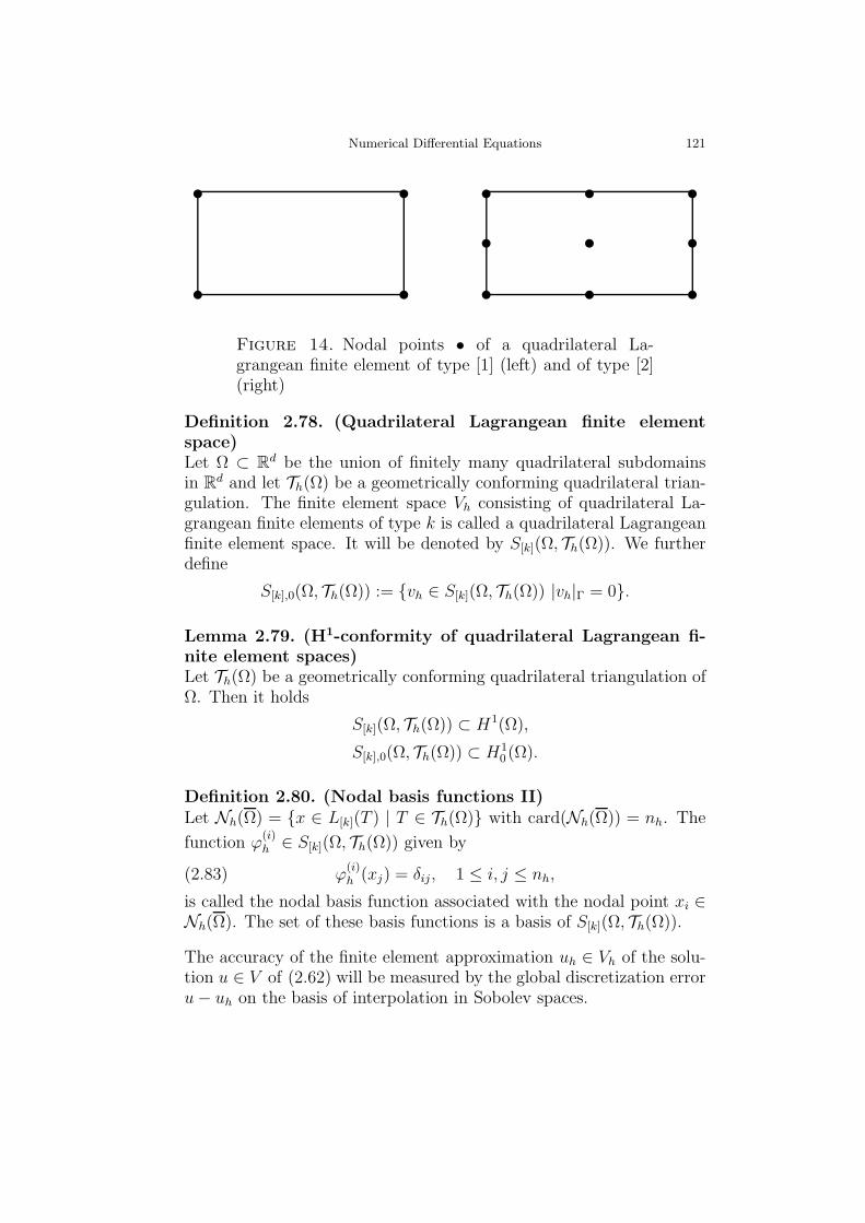
Numerical Differential Equations 121
Figure 14. Nodal points • of a quadrilateral La-grangean finite element of type [1] (left) and of type [2](right)
Definition 2.78. (Quadrilateral Lagrangean finite elementspace)Let Ω ⊂ Rd be the union of finitely many quadrilateral subdomainsin Rd and let Th(Ω) be a geometrically conforming quadrilateral trian-gulation. The finite element space Vh consisting of quadrilateral La-grangean finite elements of type k is called a quadrilateral Lagrangeanfinite element space. It will be denoted by S[k](Ω, Th(Ω)). We furtherdefine
S[k],0(Ω, Th(Ω)) := vh ∈ S[k](Ω, Th(Ω)) |vh|Γ = 0.
Lemma 2.79. (H1-conformity of quadrilateral Lagrangean fi-nite element spaces)Let Th(Ω) be a geometrically conforming quadrilateral triangulation ofΩ. Then it holds
S[k](Ω, Th(Ω)) ⊂ H1(Ω),
S[k],0(Ω, Th(Ω)) ⊂ H10 (Ω).
Definition 2.80. (Nodal basis functions II)Let Nh(Ω) = x ∈ L[k](T ) | T ∈ Th(Ω) with card(Nh(Ω)) = nh. The
function ϕ(i)h ∈ S[k](Ω, Th(Ω)) given by
ϕ(i)h (xj) = δij, 1 ≤ i, j ≤ nh,(2.83)
is called the nodal basis function associated with the nodal point xi ∈Nh(Ω). The set of these basis functions is a basis of S[k](Ω, Th(Ω)).
The accuracy of the finite element approximation uh ∈ Vh of the solu-tion u ∈ V of (2.62) will be measured by the global discretization erroru− uh on the basis of interpolation in Sobolev spaces.
122 Ronald H.W. Hoppe
Definition 2.81. (Local and global interpolation operator)Let Th(Ω) be a geometrically conforming simplicial triangulation ofΩ ⊂ R
d and let (T, PT ,ΣT ), T ∈ Th(Ω), be a simplicial Lagrangeanfinite element of type k, where PT = Pk(T ) with dimPT = nk and
ΣT = p(xi) | xi ∈ Lk(T ), 1 ≤ i ≤ nk. Further, let ϕ(i)T , 1 ≤ i ≤ nk,
be the nodal basis functions associated with the nodal points xi. Theoperator IT : V ∩ C(T ) → PT given by
ITv :=
nk∑
i=1
v(xi) ϕ(i)T , v ∈ V ∩ C(T )(2.84)
is called the local interpolation operator. If Vh is the associated simpli-cial Lagrangean finite element space, the operator Ih : V ∩C(Ω) → Vhgiven by
Ihv|T := IT v|T , T ∈ Th(Ω)(2.85)
is called the global interpolation operator.
We now assume that the solution u ∈ V of (2.62) satisfies u ∈ V ∩Hk+1(Ω) with k ∈ N sufficiently large such that Hk+1(Ω) ⊂ C(Ω).Then Ihu is well defined and Cea’s Lemma (cf. Lemma ??) implies
‖u− uh‖1,Ω ≤ C
α‖u− Ihu‖1,Ω.(2.86)
In order to estimate the global interpolation error ‖u− Ihu‖1,Ω, takingadvantage of the definition of Ih and of PT = Pk(T ) ⊂ H1(T ), T ∈Th(Ω), we obtain
‖u− Ihu‖1,Ω =( ∑
T∈Th(Ω)
‖u− ITu‖21,T)1/2
,(2.87)
i.e., we obtain an estimate of the global interpolation error by meansof estimates of the local interpolation errors ‖u− ITu‖1,T , T ∈ Th(Ω).
Lemma 2.82. (Estimate of the local interpolation operator)
Let (T , Pk(T ), ΣT ) be the simplicial Lagrangean reference element of
type (k) with k ∈ N such that Hk+1(T ) is continuously embedded in
C(T ). Further, let (T, Pk(T ),ΣT ) be a simplicial Lagrangean finite
element of type (k) which is affine equivalent to (T , Pk(T ), ΣT ) withρ(T ) denoting the radius of the largest ball that can be inscribed inT . Then there exists a constant C > 0 which only depends on thereference element such that
|v − ITv|1,T ≤ Chk+1T
ρT|v|k+1,T , v ∈ Hk+1(T ).(2.88)

Numerical Differential Equations 123
Proof. We refer to Ciarlet.
Now, letH be a null sequence of positive real numbers and let Th(Ω)Hbe a family of geometrically conforming simplicial triangulations ofΩ. The estimate (2.88) shows that the estimate (2.87) of the globalinterpolation error depends in such a way on the triangulations thatthe right-hand side in (2.87) is unbounded, if hT /ρT → ∞, T ∈ Th(Ω)as h → 0. In order to exclude this case, we have to impose a furthercondition on Th(Ω)H.
Definition 2.83. (Shape regularity)The family Th(Ω)H of geometrically conforming simplicial triangula-tion is called shape regular, if there exists a constant σ > 0, indepen-dent of hT , T ∈ Th(Ω), such that for all T ∈ Th(Ω), h ∈ H it holds
hTρT
≤ σ.(2.89)
We are now in a position to provide an a priori error estimate of theglobal discretization error in the ‖ · ‖1,Ω-norm.
Theorem 2.84. (A priori error estimate in the H1-norm I)Let Th(Ω)H be a shape regular family of geometrically conformingsimplicial triangulations of Ω and let VhH be the associated fam-ily of finite element spaces based on simplicial Lagrangean finite ele-ments of type k with k such that the embeddings Hk+1(Ω) → C(Ω) and
Hk+1(T ) → C(T ) are continuous. If u ∈ V is the solution of (2.62)with u ∈ V ∩ Hk+1(Ω) and if uh ∈ Vh, h ∈ H, are the solutions of(2.68), then there exists a constant C > 0, depending only on the localgeometry of the triangulations, such that
‖u− uh‖1,Ω ≤ C hk |u|k+1,Ω.(2.90)
Proof. The proof follows readily from (2.86),(2.87),(2.88), and (2.89).
For so-called (k + 1)-regular variational equations we obtain upperbounds that only depend on h and on the data of the problem.
Definition 2.85. (k-regularity)The variational equation (2.62) with
ℓ(v) = (f, v)0,Ω, f ∈ L2(Ω)

124 Ronald H.W. Hoppe
is called k-regular, k ≥ 2, if its solution satisfies u ∈ V ∩Hk+1(Ω) andif there exists a constant C > 0, independent of h, such that
‖u‖k,Ω ≤ C ‖f‖0,Ω.(2.91)
Corollary 2.86. (A priori error estimate in the H1-norm II)Under the assumptions of Theorem 2.84 suppose that the solution uof (2.62) is (k + 1)-regular. Then, there exists a constant C > 0,depending only on the local geometry of the triangulation, such that
‖u− uh‖1,Ω ≤ C hk ‖f‖0,Ω.(2.92)
Since ‖v‖0,Ω ≤ ‖v‖1,Ω, v ∈ V, the estimate (2.92) implies ‖u− uh‖0,Ω =O(hk). However, the estimation ‖Ihu − u‖0,Ω = O(hk+1) of the in-terpolation error suggests that this estimate is not optimal. In fact,under certain assumptions the optimal order O(hk+1) can be shown.The theoretical background of an optimal a priori error estimate in theL2-norm is given by the Lemma of Aubin and Nitsche, also known asNitsche’s trick.
Theorem 2.87. (Lemma of Aubin and Nitsche)Let V be a Hilbert space with inner product (·, ·)V , let a(·, ·) : V×V → R
be a bounded, V -elliptic bilinear form, and let ℓ : V → R be a boundedlinear functional. Let H be another Hilbert space with inner product(·, ·)H such that V is continuously and densely embedded in H. Further,let u ∈ V and uh ∈ Vh be the unique solutions of (2.62) and (2.68).Then it holds
(i) For each g ∈ H the adjoint variational equation
a(v, zg) = (g, v)H, v ∈ V(2.93)
admits a unique solution zg ∈ V .
(ii) There exists a constant C > 0 such that the global discretizationerror u− uh satisfies
‖u− uh‖H ≤ C ‖u− uh‖V(
supg∈H
1
‖g‖Hinf
ϕh∈Vh
‖zg − ϕh‖V)
.(2.94)
Proof. We refer to Ciarlet.
The following a priori estimate of the global discretization error in theL2-norm is an immediate consequence of the Lemma of Aubin andNitsche.

Numerical Differential Equations 125
Theorem 2.88. (A priori error estimate in the L2-norm)Let the assumptions of Theorem 2.90 be satisfied and suppose thatthe adjoint variational equation (2.93) is (k + 1)-regular. Then thereexists a constant C > 0, depending only on the local geometry of thetriangulations, such that
‖u− uh‖0,Ω ≤ C hk+1 |u|k+1,Ω.(2.95)
Proof. The proof follows from the Lemma of Aubin and Nitsche withH = L2(Ω). In particular, it follows from Corollary 2.86 and the(k + 1)-regularity of the adjoint variational equation that
infϕh∈Vh
‖zg − ϕh‖1,Ω ≤ ‖zg − Ihzg‖1,Ω ≤ C h ‖zg‖k+1,Ω ≤ C h ‖g‖0,Ω.
Hence, from (2.94) we deduce
‖u− uh‖0,Ω ≤ C h ‖u− uh‖1,Ω.Theorem 2.84 provides a further estimate of the right-hand side whichallows to conclude.
Remark 2.89. (A priori error estimate in the L∞-norm)For an optimal a priori error estimate of the global discretization errorin the L∞-norm we refer to Ciarlet.
126 Ronald H.W. Hoppe
2.3 The heat equation
2.3.1 Preliminaries
We consider an initial-boundary value problem for the heat equation(??) in Q := Ω × (0, T ), where Ω is a bounded domain in Rd withboundary Γ := ∂Ω, and T ∈ R+. We set Σ := Γ × (0, T ). We furtherassume given functions
f ∈ C(Q) , uD ∈ C(Γ× (0, T )) , u0 ∈ C(Ω),(2.96)
which satisfy the compatibility condition
uD(x, 0) = u0(x), x ∈ Γ.(2.97)
The initial-boundary value problem amounts to the computation of afunction u : Q→ R such that
ut(x, t)−∆u(x, t) = f(x, t), (x, t) ∈ Q,(2.98a)
u(x, t) = uD(x, t), (x, t) ∈ Σ,(2.98b)
u(x, 0) = u0(x), x ∈ Ω.(2.98c)
Definition 2.90. (Classical solution of the initial-boundary valueproblem for the heat equation)Under the assumptions (2.96) and (2.97), a function u ∈ C(Q) withu(x, ·) ∈ C1((0, T )) for x ∈ Ω, and u(·, t) ∈ C2(Ω) for t ∈ (0, T ),is called a classical solution of (2.98a)-(2.98c), if u pointwise satisfiesthe equations (2.98a)-(2.98c). The initial-boundary value problem issaid to be well posed, if the solution depends continuously on the dataf, uD, u0.
In the sequel we summarize the most important existence and unique-ness results for classical solutions of the initial-boundary value problem(2.98a)-(2.98c). For proofs and further results we refer to Evans.The uniqueness of a classical solution follows from the weak maximumprinciple.
Theorem 2.91. (Weak maximum principle)We suppose that (2.96) and (2.97) hold true. Further, we refer to ∂RQas the parabolic boundary ∂RQ := (Ω×0)∪(Γ×[0, T ]). If the functionu ∈ C(Q) with u(x, ·) ∈ C1((0, T )) for x ∈ Ω and u(·, t) ∈ C2(Ω) fort ∈ (0, T ) satisfies the inequality
∂u
∂t(x, t)−∆u(x, t) ≤ 0, (x, t) ∈ Q,(2.99)
Numerical Differential Equations 127
then it holds
max(x,t)∈Q
u(x, t) = max(x,t)∈∂RQ
u(x, t).(2.100)
If u1 and u2 are two classical solution, an application of Theorem 2.91to u1 − u2 and u2 − u1 yields u1 = u2, i.e., it holds:
Corollary 2.92. (Uniqueness of a classical solution)Under the assumptions (2.96) and (2.97), the initial-boundary valueproblem (2.98a)-(2.98c) admits a unique classical solution.
Remark 2.93. (Growth condition)In case Ω = Rd the boundary condition (2.98b) has to be replaced bythe growth condition
u(x, t) = O(exp(−λ|x|2)) for |x| → ∞ (λ > 0)(2.101)
The existence of a classical solution follows from an explicit represen-tation with respect to the data f, uD, u0 by means of a kernel functionof the heat equation.
Definition 2.94. (Kernel function of the heat equation)Let Ω ⊆ Rd. A function K : Ω×Ω×R+ → R is called a kernel functionof the heat equation, if it holds
(i)∂
∂tK(x, y, t)−∆xK(x, y, t) = 0, (x, y, t) ∈ Ω× Ω× R+,
(ii) K(x, y, t) = 0, (x, y, t) ∈ Γ× Ω× R+,
(iii) limt→0
∫
Ω
K(x, y, t)v(x) dx = v(y), y ∈ Ω, v ∈ C(Ω).
The existence of a kernel function can be shown by means of a funda-mental solution of the heat equation
Λ(x, y, t) := (4πt)−d/2 exp(−|x− y|24t
), (x, y, t) ∈ Rd × R
d × R+.
(2.102)
For a bounded function u0 ∈ C(Rd) let u : Rd×R+ → R be the functiondefined by the convolution
u(x, t) = Λ(x, ·, t) ∗ u0(·) =∫
Rd
Λ(x, y, t)u0(y) dy.
128 Ronald H.W. Hoppe
Then u ∈ C∞(Rd × R+) and u solves the heat equation in Rd × R+
with the initial condition u(x, 0) = u0(x), x ∈ Ω. In fact, computingthe partial derivatives ∂Λ/∂t and ∂2Λ/∂xi∂xj , 1 ≤ i, j ≤ d, one easilyverifies that Λ (as a function of x) satisfies the heat equation in (x, t) ∈Rd × R+. It follows that
∂
∂tu(x, t) = (
∂
∂tΛ(x, ·, t)) ∗ u0(·) = (∆xΛ(x, ·, t)) ∗ u0(·) = ∆xu(x, t).
Since Λ ∈ C∞(Rd×Rd×R+), differentiation shows that u ∈ C∞(Rd×R+).
In case of a bounded C2-domain Ω ⊂ Rd, the fundamental solution pro-vides an explicit representation of the solution of the initial-boundaryvalue problem (2.98a)-(2.98c) with homogeneous initial conditions u0 ≡0. This allows to deduce the existence of a kernel function.
Theorem 2.95. (Kernel function for a bounded spatial domain)
Let Ω ⊂ Rd be a bounded C2-domain. Then the heat equation admitsa kernel function K ∈ C∞(Ω × Ω × R+) such that K(x, y, t) > 0 andK(x, y, t) = K(y, x, t), (x, y, t) ∈ Ω× Ω× R+.
The kernel function K from Theorem 2.95 gives rise to the followingrepresentation of the unique classical solution of the initial-boundaryvalue problem (2.98a)-(2.98c):
Theorem 2.96. (Classical solution of the initial-boundary va-lue problem for the heat equation)Let Ω ⊂ Rd be a bounded C2-domain and suppose that the conditions(2.96) and (2.97) are satisfied. Then the initial-boundary value problem(2.98a)-(2.98c) admits a unique classical solution u ∈ C(Q) ∩ C∞(Q)which has the explicit representation
u(x, t) =
t∫
0
∫
Ω
K(x, y, t− s)f(y, s) dy ds +
∫
Ω
K(x, y, t)u0(y) dy −t∫
0
∫
Γ
νΓ · ∇yK(x, y, t− s)uD(y, s) dσ(y) ds.
Remark 2.97. (Compatibility condition)If the compatibility condition (2.97) is not satisfied, one can show theexistence of a unique classical solution u ∈ C((Ω× R+) \ (Γ× 0)) ∩C∞(Q) with the same representation as in Theorem 2.96.

Numerical Differential Equations 129
Theorem 2.96 shows the well posedness of the initial-boundary valueproblem (2.98a)-(2.98c) and reflects the smoothing property of the par-abolic differential operator. The solution satisfies u ∈ C∞(Q) in Q,even if the initial and boundary data are only continuous functions.
Remark 2.98. (General initial-boundary value problems)As far as more general initial-boundary value problems for linear secondorder parabolic differential equations are concerned, we refer to Evans.

130 Ronald H.W. Hoppe
2.3.2 Method of lines and Rothe’s method
The numerical solution of the initial-boundary value problem (2.98a)-(2.98c) can be done on the basis of a semi-discretization in space orin time. The semi-discretization in space is called the method of lines.We consider an equidistant grid point set
Ωh := x = (xν1, · · · , xνd)Tof step size h > 0 and refer to Ωh and Γh as the sets of interior andboundary grid points. Assume fh(t) ∈ C(Ωh), t ∈ (0, T ], uDh ∈ C(Γh),and u0h ∈ C(Ωh) to be approximations of f, uD, and u0. Then themethod of lines requires the solution of the following initial value prob-lem for a system of first order ordinary differential equations
(uh)t −∆huh = fh(t), t ∈ (0, T ),(2.103a)
uh(0) = u0h(2.103b)
in the unknowns uh(x), x ∈ Ωh. Typically, this system is stiff so that thenumerical integration of (2.103a),(2.103b) requires the use of implicitor semi-implicit methods (cf. Chapter 1).The semi-discretization in time is called Rothe’s method. We consideran equidistant partition
Ik := tm := mk , k := T/(M + 1), M ∈ N(2.104)
of the time interval [0, T ] of step size k > 0 and discretize (2.98a)implicitly in time, e.g., by means of the implicit Euler method. Then,for each time step we have to solve a boundary value problem for alinear second order elliptic differential equation
(I − k∆u(tm) = u(tm−1) + kf(tm) in Ω,(2.105a)
u(·, tm) = uD(tm) on Γ.(2.105b)
For the numerical solution of (2.105a),(2.105b) we can use the tech-niques presented in subsections 2.2.2 and 2.2.3.

Numerical Differential Equations 131
2.3.3 Finite difference approximations
We consider finite difference approximations in space and time withrespect to a grid point set
Qh,k := Ωh × Ik.(2.106)
ForDh,k ⊆ Qh,k we refer to C(Dh,k) as the linear space of grid functionsin Dh,k.For grid functions uh,k ∈ C(Qh,k) we define the forward difference quo-tient
D+k uh,k(x, t) := k−1
(
uh,k(x, t + k)− uh,k(x, t))
,(2.107)
where x ∈ Ωh, t ∈ Ik \ T, and the backward difference quotient
D−k uh,k(x, t) := k−1
(
uh,k(x, t)− uh,k(x, t− k))
,(2.108)
where x ∈ Ωh, t ∈ Ik \ 0. Moreover, let fh,k ∈ C(Qh,k), uDh ∈ C(Γh ×
Ik), and u0h ∈ C(Ωh) be approximations of f, ud, and u0.
Definition 2.99. (Explicit Euler method)Using the forward difference quotient, we obtain the explicit Eulermethod
uh,k(x, t + k) = (I + k∆h)uh,k(x, t) + kfh,k(x, t),(2.109a)
x ∈ Ωh, t ∈ Ik \ T,uh,k(x, t + k) = uDh (x, t + k), x ∈ Γh, t ∈ Ik \ T,(2.109b)
uh,k(x, 0) = u0h(x), x ∈ Ωh.(2.109c)
Definition 2.100. (Implicit Euler method)The use of the backward difference quotient gives rise to the implicitEuler method
(I − k∆h)uh,k(x, t) = uh,k(x, t− k) + kfh,k(x, t),(2.110a)
x ∈ Ωh, t ∈ Ik \ 0,uh,k(x, t) = uD(x, t), x ∈ Γh, t ∈ Ik \ 0,(2.110b)
uh,k(x, 0) = u0h(x), x ∈ Ωh.(2.110c)
If uh,k(x, t) is known in x ∈ Ωh, t = tm, 0 ≤ m ≤ M, for the explicitEuler method (2.109a)-(2.109c) we obtain uh,k(x, t) in x ∈ Ωh, t =tm+1, by the evaluation of the right-hand side in (2.109a). However,knowing uh,k(x, t) in x ∈ Ωh, t = tm−1, 1 ≤ m ≤ M, for the implicit
132 Ronald H.W. Hoppe
Euler method (2.110a)-(2.110c) the computation of uh,k(x, tm), x ∈ Ωh,requires the solution of a linear algebraic system.
Definition 2.101. (Θ-Method)We multiply (2.110a) (with t + k instead of t) with some Θ ∈ [0, 1],multiply (2.109a) with 1−Θ, and add the resulting equations. Denotingby LΘ
h,k the difference operator
LΘh,kuh,k := Θ∆huh,k(·, t+ k) + (1−Θ)∆huh,k(·, t)
and by fΘh,k the grid function
fΘh,k := Θfh,k(·, t+ k) + (1−Θ)fh,k(·, t),
we obtain the so-called Θ-method:
k−1(uh,k(·, t+ k)− uh,k(·, t)) −(2.111a)
LΘh,kuh,k = fΘ
h,k, x ∈ Ωh, t ∈ Ik \ T,uh,k(x, t) = uDh (x, t), x ∈ Γh, t ∈ Ik \ 0,(2.111b)
uh,k(x, 0) = u0h(x), x ∈ Ωh.(2.111c)
For Θ = 0 we recover the explicit Euler method (2.109a)-(2.109c),whereas Θ = 1 yields the implicit Euler method (2.110a)-(2.110c). Theimplicit scheme for Θ = 1/2 is called the Crank-Nicolsen method.
For the definition of the convergence of the finite difference approxima-tions we measure the global discretization error eh,k := u|Qh,k
− uh,k in
a suitable norm ‖ · ‖h,k of the linear space C(Qh,k) of grid functions in
Qh,k. An example is the discrete maximum norm
‖uh,k‖h,k := max(x,t)∈Qh,k
|uh,k(x, t)|.
Definition 2.102. (Convergence of the Θ-method)Let u be the classical solution of the initial-boundary value problemfor the heat equation and let uh,k ∈ C(Qh,k) be the solution of theΘ-method. The Θ-method is said to be convergent, if
‖u− uh,k‖h,k → 0 as h, k → 0.
The Θ-method is said to be convergent of order p1 in h and p2 in k, ifthere exists a constant C > 0, independent of h and k, such that forsufficiently small h, k it holds
‖u− uh,k‖h,k ≤ C (hp1 + kp2).

Numerical Differential Equations 133
As in the numerical solution of initial value problems for ordinary dif-ferential equations (cf. Chapter 1), sufficient conditions for the con-vergence are given by the consistency of the Θ-method with the giveninitial-boundary value problem and by the stability of the Θ-method.
Definition 2.103. Consistency of the Θ-method)Under the assumptions of Definition 2.102 the grid function
τh,k(x, t) :=
D+k u(x, t)− LΘ
h,ku(x, t)− fh,k(x, t) , (x, t) ∈ Ωh × (Ik \ 0)u(x, t)− uDh,k(x, t) , (x, t) ∈ Γh × (Ik \ 0)u(x, 0)− u0h(x) , x ∈ Ωh
is called the local discretization error. The Θ-method is said to beconsistent with the initial-boundary value problem, if
‖τh,k‖h,k → 0 as h, k → 0.
The Θ-method is said to be consistent of order p1 in h and p2 in k, ifthere exists a constant C > 0, independent of h and k, such that forsufficiently small h, k it holds
‖τh,k‖h,k ≤ C (hp1 + kp2).
Under the assumption of smooth data and a sufficiently smooth clas-sical solution, the consistency and the order of consistency of the Θ-method can be derived by multidimensional Taylor expansion.
Theorem 2.104. Order of consistency of the Θ-method)We consider the Θ-method (2.111a)-(2.111c) with fh,k = f |Qh,k
, uDh =uD|Γh×Ik , and u
0h = u0|Ωh
. We assume that the classical solution satis-
fies u ∈ C2([0, T ];C4(Ω)). Then it follows by multidimensional Taylorexpansion that for Θ 6= 1/2 the order of consistency of the Θ-method isp1 = 2 in h and p2 = 1 in k. Note that for the explicit Euler method theTaylor expansion is around (x, t), whereas for the implicit methods theTaylor expansion is around (x, t+ k). If the classical solution satisfiesu ∈ C3([0, T ];C4(Ω)), the Crank-Nicolsen method (Θ = 1/2) has theorder of consistency p1 = 2 in h and p2 = 2 in k. In this case, theTaylor expansion is around (x, t + k/2).
The stability of the Θ-method means continuous dependence of thesolution uh,k on the data fh,k, u
Dh,k, and u
0h.
134 Ronald H.W. Hoppe
Definition 2.105. (Stability of the Θ-method)Let uh,k and zh,k be the solutions of the Θ-method (2.111a)-(2.111c)with respect to the ’unperturbed’ data fh,k, u
Dh,k, u
0h, and the ’perturbed’
data fh,k + δfh,k, uDh,k + δuDh,k, u
0h + δu0h with grid functions δgh,k ∈
C(Qh,k), δuDh,k ∈ C(Γh × Ik), δu
0h ∈ C(Ωh). Then the Θ-method is
said to be stable for (h, k) ∈ Λ ⊆ R+ × R+, if for each ε > 0 thereexists δ = δ(ε, h, k) > 0 such that
‖uh,k − zh,k‖h,k < ε
for all perturbations δu0h and (δgh,k, δuDh,k) satisfying
‖δu0h‖h + ‖(δfh,k, δuDh,k)‖h,k < δ.
The set Λ is called the stability region. If Λ = R+×R+, the Θ-methodis said to be unconditionally stable, otherwise it is called conditionallystable.
As in case of finite difference approximations of elliptic boundary valueproblems, the stability of the consistent Θ-method is sufficient for theconvergence.
Theorem 2.106. (Sufficient condition for convergence)Assume that the Θ-method is consistent with the initial-boundary valueproblem. If the Θ-method is stable, it is convergent and the order ofconvergence corresponds to the order of consistency.
Proof. The solution u of the initial-boundary value problem satisfiesthe difference equations
D+k u(x, t)− LΘ
h,ku(x, t) = fΘh,k(x, t) + τh,k(x, t), x ∈ Ωh, t ∈ Ik \ 0,
u(x, t) = uDh,k(x, t) + τh,k(x, t), x ∈ Γh, t ∈ Ik \ 0,u(x, 0) = u0h(x) + τh,k(x, 0), x ∈ Ωh.
Setting δfh,k(x, t) = τh,k(x, t), x ∈ Ωh, t ∈ Ik\0, δuDh,k = τh,k(x, t), x ∈Γh, t ∈ Ik \ 0, and δu0h(x) = τh,k(x, 0), x ∈ Ωh, and taking the con-sistency ‖τh,k‖h,k → 0 as h, k → 0 into account, the assertion followsfrom the Definition 2.105.
Remark 2.107. (Stability)We note that in the literature there is a wide variety of stability notionsfor finite difference approximations of parabolic initial-boundary valueproblems (cf., e.g, Thomas).Theorem 2.106 is sometimes referred to as the Theorem of Lax. Under
Numerical Differential Equations 135
the same assumptions, it can be shown that the stability is also neces-sary for the convergence of the Θ-method. The equivalence of the sta-bility and the convergence of consistent finite difference approximationsof parabolic initial-boundary value problems is called the equivalencetheorem of Lax and Richtmyer (for a proof we refer to Strikwerda).
Since the Θ-method corresponds to a linear algebraic system, the stabil-ity can be established by arguments from numerical linear algebra. Tothis end, we assume Ω = (a, b)2, a, b ∈ R, a < b. If Ωh = x1, · · · , xnh
)T
and if u(m)h denotes the vector u
(m)h = (uh,k(x1, tm), · · · , uh,k(xnh
, tm))T ,
0 ≤ m ≤ M + 1, the Θ-method is equivalent to the linear algebraicsystem
(Ih + kBh(Θ))u(m)h = (Ih − kCh(Θ))u
(m−1)h + b
(m)h ,(2.112)
where Bh(Θ) = ΘAh, Ch(Θ) = (1 − Θ)Ah with the block tridiagonal
matrix Ah ∈ Rnh×nh from (2.41) and the vector b(m)h ∈ Rnh . If δu
(0)h ∈
Rnh and δb(m)h ∈ Rnh, 1 ≤ m ≤ M + 1, are perturbations in the initial
condition and the right-hand side, and if z(m)h is the solution of (2.112)
with respect to the perturbed data, by induction on m it can be shownthat
‖u(m)h − z
(m)h ‖ ≤ ‖Dh(Θ)‖m‖δu(0)h ‖ +
(2.113)
m−1∑
ℓ=0
‖Dh(Θ)‖m−ℓ−1‖(Ih + kBh(Θ))−1‖‖δb(ℓ)h ‖,
where Dh(Θ) := (Ih + kBh(Θ))−1(Ih − kCh(Θ)) and the matrix normis the norm associated with the Euclidean vector norm. The estimate(2.113) implies that for stability it suffices to show ρ(Dh(Θ)) < 1,where ρ(Dh(Θ)) is the spectral radius of DH(Θ). The knowledge ofthe eigenvalues of Ah (cf. (2.43)) enables to compute the eigenvalues ofDh(Θ). For Θ < 1/2, the step size restriction k ≤ h2(2 − 4Θ) impliesρ(Dh(Θ) < 1, whereas for Θ ≥ 1/2 we have ρ(DH(Θ) < 1 withoutconditions on the step sizes. Hence, the Θ-method is conditionallystable for Θ < 1/2 and unconditionally stable for Θ ≥ 1/2.
For further results on the stability of finite difference approximationsof parabolic initial-boundary value problems we refer to Gustafsson/Kreiss/Oliger, Richtmyer/Morton, Strikwerda, and Thomas.

136 Ronald H.W. Hoppe
2.3.4 Finite element approximations
Finite element approximations of initial-boundary value problems forthe heat equation
∂u
∂t−∆u = f in Q,(2.114a)
u = 0 on Σ,(2.114b)
u(·, 0) = u0 in Ω,(2.114c)
are based on the concept of a weak solution. Here, Ω ⊂ Rd is supposed
to be a bounded Lipschitz-domain with boundary Γ = ∂Ω. Moreover,we assume
f ∈ L2((0, T ), L2(Ω)), u0 ∈ L2(Ω).(2.115)
We note that for Hilbert spaces H with norm ‖ · ‖H and V with norm‖ ·‖V such that V is continuously and densely embedded in H , we referto 〈·, ·〉V ∗,V the dual product of V ∗ and V . We refer to L2((0, T );H)as the Hilbert space with norm
‖u‖L2((0,T );H) :=(
T∫
0
‖u(t)‖2H dt)1/2
,
and define L2((0, T );V ) and ‖ · ‖L2((0,T );V ) analogously. Moreover, weintroduce H1((0, T );V ∗) as the Hilbert space with the norm
‖u‖H1((0,T );V ∗) :=(
T∫
0
(
‖u(t)‖2V ∗ + ‖ut(t)‖2V ∗
)
dt)1/2
.
Definition 2.108. (Weak solution of the initial-boundary valueproblem)Under the assumptions (2.115) a function u ∈ H1((0, T );H−1(Ω)) ∩L2((0, T );H1
0(Ω)) is called a weak solution of the initial-boundary valueproblem (2.114a)-(2.114c), if for all v ∈ H1
0 (Ω) it holds
〈∂u∂t, v〉H−1(Ω),H1
0 (Ω) + (∇u,∇v)0,Ω = (f, v)0,Ω for almost all t ∈ (0, T ),
(2.116a)
(u(·, 0), v)0,Ω = (u0, v)0,Ω.(2.116b)
Remark 2.109. (Pointwise continuity in t)It can be shown that the space H1((0, T );H−1(Ω))∩L2((0, T );H1
0(Ω))
Numerical Differential Equations 137
is continuously embedded in C([0, T ];L2(Ω)). Hence, u(·, 0) in (2.116b)is well defined. For a proof we refer to Renardy/Rogers.
Theorem 2.110. (Existence and uniqueness of a weak solution)
Under the assumptions (2.115) the initial-boundary value problem(2.114a)-(2.114c) admits a unique weak solution.
Proof. We refer to Renardy/Rogers.
The standard finite element method for the computation of a weaksolution relies on a discretization in the spatial variables by restricting(2.116a),(2.116b) to a finite element space Vh ⊂ H1
0 (Ω) with dim Vh =nh. We are looking for uh ∈ Vh such that for all vh ∈ Vh it holds
(∂uh∂t
, vh)0,Ω + (∇uh,∇vh)0,Ω = (f(t), vh)0,Ω,(2.117a)
(uh(0), vh)0,Ω = (u0, vh)0,Ω.(2.117b)
The finite element approximation (2.117a),(2.117b) represents an ini-tial value problem for a system of linear first order ordinary differ-
ential equations. If (ϕ(i)h )nh
i=1 is a basis of Vh, the solution uh(t) ∈Vh, t ∈ [0, T ], is of the form uh(t) =
∑nh
j=1 yj(t)ϕ(j)h . Hence, for y(t) =
(y1(t), · · · , ynh(t))T we obtain
Mhdy(t)
dt+ Ahy(t) = bh(t), t ∈ (0, T ],(2.118a)
y(0) = y0 .(2.118b)
Here, Mh ∈ Rnh×nh stands for the mass matrix
Mh :=
(ϕ(1)h , ϕ
(1)h )0,Ω · · · (ϕ
(nh)h , ϕ
(1)h )0,Ω
· · · · ·· · · · ·
(ϕ(1)h , ϕ
(nh)h )0,Ω · · · (ϕ
(nh)h , ϕ
(nh)h )0,Ω
(2.119)
and Ah ∈ Rnh×nh refers to the stiffness matrix
Ah :=
(∇ϕ(1)h ,∇ϕ(1)
h ) · · · (∇ϕ(nh)h ,∇ϕ(1)
h )· · · · ·· · · · ·
(∇ϕ(1)h ,∇ϕ(nh)
h ) · · · (∇ϕ(nh)h ,∇ϕ(nh)
h )
,(2.120)

138 Ronald H.W. Hoppe
whereas the vectors bh(t) ∈ Rnh, t ∈ [0, T ], and y0 ∈ Rnh, y0 = (y01, · · · ,y0nh
)T are given by
bh(t) := ((f(t), ϕ(1)h )0,Ω, · · · , (f(t), ϕ(nh)
h )0,Ω)T ,(2.121a)
y0j = (u0, ϕ(j)h )0,Ω, 1 ≤ j ≤ nh.(2.121b)
For the discretization in time we consider a partition Ik of the timeinterval [0, T ] according to (2.104) and approximate the time derivativeby the forward difference quotient, by the backward difference quotient,or by a convex combination of both as in the Θ-method (cf. Definition
2.101). We are looking for functions u(m)h,k ∈ Vh, 0 ≤ m ≤ M + 1, such
that
k−1Mh(u(m+1)h,k − u
(m)h,k ) + ΘAhu
(m+1)h,k +(2.122a)
+ (1−Θ)Ahu(m)h,k = bΘh (tm, tm+1), 0 ≤ m ≤M ,
uh,0 = u0h,(2.122b)
where bΘh (tm, tm+1) := Θbh(tm+1)+(1−Θ)bh(tm) and u0h =
∑nh
j=1 y0jϕ
(j)h .
As far as a priori estimates of the global discretization error eh,k(t) :=u(t)−uh,k(t), t ∈ Ik, are concerned, we assume that for v ∈ Hr+1(Ω), r ∈N, the finite element spaces Vh satisfy the approximation property
infvh∈Vh
(
‖v − vh‖0,Ω + h ‖v − vh‖1,Ω)
≤ Chr+1,(2.123)
where C > 0 is a constant independent of h. If we use the backwarddifference quotient in time, i.e., Θ = 1 in (2.122a), we have the followinga priori error estimate in the H1-seminorm which is a norm on H1
0 (Ω).
Theorem 2.111. (A priori error estimate in the H1-seminormfor the implicit Euler method)Let u ∈ H1((0, T );Hr+1(Ω)) ∩ H2((0, T );L2(Ω)), r ∈ N, the weak so-lution of the initial-boundary value problem and let uh,k be the solu-tion of (2.122a),(2.122b) for Θ = 1. We further assume (2.123) and|u0−u0h|1,Ω = O(hr). Then, there exists a constant C > 0, independentof h, k, such that for all 0 ≤ m ≤M + 1 it holds
|u(tm)− uh,k(tm)|1,Ω ≤ C(hr + k).(2.124)
Proof. We refer to Thomee.
Under stronger regularity assumptions on the weak solution, for theCrank-Nicolsen method, i.e., Θ = 1/2, we obtain convergence of order2 in k.

Numerical Differential Equations 139
Theorem 2.112. (A priori error estimate in the H1-seminormfor the Crank-Nicolsen method)Assume that the weak solution satisfies
u ∈ H1((0, T );Hr+1(Ω)) ∩H2((0, T );H2(Ω)) , ∆utt ∈ L2((0, T );L2(Ω)).
Further, let uh,k be the solution of (2.122a),(2.122b) for Θ = 1/2 andsuppose that (2.123) and |u0 − u0h|1,Ω = O(hr) hold true. Then, thereexists a constant C > 0, independent of h, k, such that for all 0 ≤ m ≤M + 1 it holds
|u(tm)− uh,k(tm)|1,Ω ≤ C(hr + k2).(2.125)
Proof. We refer to Thomee.
We recall Theorem 2.87 which provides a quasi-optimal a priori errorestimate in the L2-norm for (r + 1)-regular elliptic boundary valueproblems. This result also holds true for the heat equation.
Theorem 2.113. (A priori error estimates in the L2-norm forthe Θ-method)In addition to the assumptions of Theorem 2.111 and Theorem 2.112suppose that the boundary value problem for the Poisson equation (2.11)is (r + 1)-regular. Then there exists a constant C > 0, independent ofh, k, such that for all 0 ≤ m ≤M + 1 it holds
‖u(tm)− uh,k(tm)‖0,Ω ≤ C(hr+1 + kp)(2.126)
with p = 1 for Θ = 1 and p = 2 for Θ = 1/2.
Proof. We refer to Thomee.
Remark 2.114. (A priori error estimate in the L∞-norm)For a priori error estimates in the L∞-norm we refer to Thomee.
140 Ronald H.W. Hoppe
2.4 The wave equation
2.4.1 Preliminaries
We consider the Cauchy problem for the spatially one-dimensional waveequation
∂2u
∂t2− ∂2u
∂x2= 0, (x, t) ∈ R× R,(2.127a)
u(x, 0) = u0(x),∂u
∂t(x, 0) = u1(x), x ∈ R,(2.127b)
where u0 and u1 are given functions in R.Introducing the coordinate transformation
ξ = t+ x, η = x− t,(2.128)
and the function
v(ξ, η) := u(1
2(ξ + η),
1
2(ξ − η)),(2.129)
it is easy to see that v satisfies the partial differential equation
∂2v
∂ξ∂η= 0, (ξ, η) ∈ R× R.(2.130)
Integration with respect to η implies the existence of a function g1 =g1(ξ) such that ∂v
∂ξ(ξ, η) = g1(ξ) and a further integration with respect
to ξ implies the existence of functions g1 = g1(ξ) and g2 = g2(η) suchthat v(ξ, η) = g1(ξ) + g2(η). Hence, it follows from (2.128) and (2.129)that any solution of (2.127a) is of the form
u(x, t) = g1(x− t) + g2(x− t).(2.131)
This result enables us to provide the following representation of thesolution of the Cauchy problem (2.127a),(2.127b).
Theorem 2.115. (Solution of the Cauchy problem for the spa-tially one-dimensional wave equation)Suppose that u0 ∈ C2(R), u1 ∈ C1(R). Then, the unique solution ofthe Cauchy problem for the spatially one-dimensional wave equation(2.127a),(2.127b) is given by
u(x, t) =1
2
x+t∫
x−t
u1(s) ds+∂
∂t
(1
2
x+t∫
x−t
u0(s) ds)
.(2.132)
Proof. According to (2.131) the solution u satisfies
u(x, t) = g1(x− t) + g2(x− t),∂u
∂t(x, t) = g′1(x+ t)− g′2(x− t).

Numerical Differential Equations 141
Setting t = 0, we obtain the system of equations
g1(x) + g2(x) = u0(x), g′1(x)− g′2(x) = u1(x),
which has the unique solution
g1(x) =1
2
x∫
0
u1(s) ds+1
2
(
g1(0)− g2(0))
+1
2u0(x),
g2(x) =1
2u0(x)−
1
2
x∫
0
u1(s) ds−1
2
(
g1(0)− g2(0))
.
The assertion is an immediate consequence of these two equations.
t
xx0 − t0 x0 x0 + t0
(x0, t0)
D
Figure 15. Domain of dependence and domain of influence.
Definition 2.116. (Domain of dependence and domain of in-fluence)It follows from (2.132) that for (x0, t0) ∈ R2 the solution u in
D = D(x0, t0) := (x, t) ∈ R2 | 0 ≤ t ≤ t0, (t− t0)
2 − (x− x0)2 ≥ 0
is uniquely determined by the initial values in the interval
I = I(x0, t0) := [x0 − t0, x0 + t0].
D is called the domain of dependence and I is said to be the domainof influence (cf. Figure 15).
142 Ronald H.W. Hoppe
Remark 2.117. (Finite speed of propagation)It also follows from (2.132) and Figure 15 that the Cauchy data prop-agate with finite speed. This is in contrast to the heat equation wherethe Cauchy data propagate with infinite speed.
The representation formula (2.132) for the solution of the Cauchy prob-lem for the spatially one-dimensional wave equation can be generalizedto higher dimensions d > 1, i.e., for the Cauchy problem
∂2u
∂t2−∆u = 0, (x, t) ∈ R
d × R+,(2.133a)
u(x, 0) = u0(x),∂u
∂t(x, 0) = u1(x), x ∈ R
d,(2.133b)
where u0 and u1 are given functions in Rd.However, we have to distinguish between d even and d odd. We referto Sd−1 as the unit sphere in Rd and to |Sd−1| as the area of Sd−1 whichis given by
|Sd−1| = 2πd/2
Γ(d/2),
where Γ stands for the Gamma function Γ(x) :=∞∫
0
sx−1 exp(−s) ds.Moreover, for a map g in Rd we introduce the function
M(x, t, g) :=1
|Sd−1|
∫
Sd−1
g(x+ tξ) dσ(ξ).
Theorem 2.118. (Solution of the Cauchy problem for the spa-tially d-dimensional wave equation: d odd)Assume d = 2m + 1, m ≥ 1, and u0, u1 ∈ C(d+3)/2(Rd). Then, theunique solution of the Cauchy problem (2.133a),(2.133b) is given by
u(x, t) =(m−1∏
i=1
(2i+ 1))−1 ( ∂
∂t
(1
t
∂
∂t
)(d−3)/2
(td−2 M(x, t, u0)) +
(1
t
∂
∂t
)(d−3)/2
(td−2 M(x, t, u1)))
.(2.134)
Proof. We refer to Evans.

Numerical Differential Equations 143
Theorem 2.119. (Solution of the Cauchy problem for the spa-tially d-dimensional wave equation: d even)Assume d = 2m,m ≥ 1, and u0, u1 ∈ C(d+4)/2(Rd). Then, the uniquesolution of the Cauchy problem (2.133a),(2.133b) is given by
u(x, t) =(
max(1,
m−1∏
i=1
2i))−1
·
·( ∂
∂t
(1
t
∂
∂t
)(d−2)/2 (t∫
0
sd−1
√t2 − s2
M(x, s, uo) ds)
+
(1
t
∂
∂t
)(d−2)/2 (t∫
0
sd−1
√t2 − s2
M(x, s, u1) ds))
.(2.135)
Proof. We refer to Evans.

144 Ronald H.W. Hoppe
2.4.2 Finite difference approximations
Let Ω ⊂ R2 be a bounded domain with boundary Γ = ∂Ω. For T > 0
we set Q := Ω× (0, T ) and Σ := Γ× (0, T ). Given functions f : Q→ R
and u0, u1 : Ω → R, as well as uD : Γ × (0, T ) → R, we consider thefollowing initial-boundary value problem for the wave equation
∂2u
∂t2−∆u = f, (x, t) ∈ Q,(2.136a)
u(x, t) = uD(x, t), (x, t) ∈ Σ,(2.136b)
u(x, 0) = u0(x),∂u
∂t(x, 0) = u1(x), x ∈ Ω,(2.136c)
For the finite difference approximation of (2.136a)-(2.136c) we consideran equidistant space-time grid Qh,k with spatial step size h and timestep size k (cf. (2.106)). We approximate the Laplacian ∆ by thediscrete Laplacian ∆h (cf. (2.34)) and the time derivative ∂2u/∂t2 bythe central difference quotient
D2ku(x, t) :=
u(x, t+ k)− 2u(x, t) + u(x, t− k)
k2.
For the approximation of the second initial condition ∂u(x, 0)/∂t =u1(x), x ∈ Ω, we introduce the artificial time level t−1 = −k and usethe central difference quotient
Dcku(x, 0) :=
u(x, k)− u(x,−k)2k
.
The finite difference approximation of (2.136a)-(2.136c) amounts to thecomputation of a grid function uh,k : Qh,k → R on the extended grid
Qh,k such that
D2kuh,k(x, t)−∆huh,k(x, t) = f(x, t), (x, t) ∈ Qh,k ∩Q,(2.137a)
uh,k(x, t) = uD(x, t), (x, t) ∈ Qh,k ∩ Σ,(2.137b)
uh,k(x, 0) = u0(x), Dckuh,k(x, 0) = u1(x), x ∈ Qh,k ∩ Ω.(2.137c)
From the second equation in (2.137c) we deduce
uh,k(x,−k) = uh,k(x, k)− 2ku1(x).(2.138)

Numerical Differential Equations 145
If we assume (2.137a) to hold true on the time level t0 = 0 as well andsolve for uh,k(x, k), we obtain
uh,k(x, k) =
d∑
i=1
(
(k
h)2 u0(x+ hei) + 2(1− (
k
h)2) u0(x) +(2.139)
(k
h)2 u0(x− hei)
)
− uh,k(x,−k) + k2 f(x, 0).
Combining (2.138) and (2.139) finally yields
uh,k(x, k) =1
2
d∑
i=1
(
(k
h)2 u0(x+ hei) + 2(1− (
k
h)2) u0(x) +(2.140)
(k
h)2 u0(x− hei)
)
+ k u1(x) + k2 f(x, 0).
Using the first equation in (2.137a) and (2.140) as initial conditionson the time levels t0 = 0 and t1 = k, we thus obtain an explicit finitedifference scheme where we can explicitly compute uh,k(x, tk), 2 ≤ k ≤M .
The domain of dependence of the solution uh,k(x, tm) of the finite dif-ference approximation are all grid points in
d∏
i=1
[x−mhei, x+mhei],(2.141)
whereas the domain of dependence of the exact solution u(x, tm) isgiven by
d∏
i=1
[x−mkei, x+mkei].(2.142)
For stability reasons we have to assume that the domain of dependenceof the exact solution is contained in the domain of dependence of the so-lution of the finite difference approximation, i.e., it follows from (2.141)and (2.142) that we have to require
d∏
i=1
[x−mkei, x+mkei] ⊂d∏
i=1
[x−mkei, x+mkei]
which holds true, if the step sizes h and k satisfy
k
h≤ 1.(2.143)
The stability condition (2.143) is called the Courant-Friedrichs-Levy(CFL) condition.
146 Ronald H.W. Hoppe
For sufficiently smooth exact solutions u we obtain the following con-vergence result:
Theorem 2.120. (Convergence of the finite difference approx-imation of the initial-boundary value problem for the waveequation)Assume that the exact solution u of (2.136a)-(2.136c) satisfies u ∈C4([0, T ];C(Ω))∩C([0, T ], C4(Ω)) and that the finite difference approx-imation fulfills the CFL condition (2.143). Then there exist constantsC1 > 0 and C2 > 0, independent of h, k, such that
|uh,k(x, t)− u(x, t)| ≤ C1 h2 + C2 k
2, (x, t) ∈ Qh,k.(2.144)
Numerical Differential Equations 147
2.4.3 Finite element approximations
We consider the initial-boundary value problem (2.136a)-(2.136c) withuD ≡ 0. We multiply (2.136a) by a function v ∈ H1(Q) with v(·, t) ∈H1
0 (Ω) for almost all t ∈ (0, T ), and v(x, T ) = 0, x ∈ Ω, and integrateover Q:
∫
Q
∂2u
∂t2v dx dt−
∫
Q
∆u v dx dt =
∫
Q
fv dx dt.(2.145)
Partial integration of the first integral on the left-hand side in (2.145)yields
∫
Q
∂2u
∂t2v dx dt =
T∫
0
∫
Ω
∂2u
∂t2v dx dt = −
T∫
0
∫
Ω
∂u
∂t
∂v
∂tdx dt +
(2.146)
∫
Ω
∂u(x, T )
∂tv(x, T )︸ ︷︷ ︸
= 0
dx−∫
Ω
∂u(x, 0)
∂t︸ ︷︷ ︸
= u1(x)
v(x, 0) dx.
On the other hand, for the second integral on the left-hand side in(2.145) Green’s formula (2.28) implies
∫
Q
∆u v dx dt =
T∫
0
∫
Ω
∆u v dx dt = −T∫
0
∫
Ω
∇u · ∇v dx dt +
(2.147)
T∫
0
∫
Γ
ν · ∇u v︸︷︷︸
= 0
dσ(x) dt.
The equations (2.146),(2.147) motivate the definition of a weak solutionof (2.136a)-(2.136c).
Definition 2.121. (Weak solution of the initial-boundary valueproblem for the wave equation)Assume that u0, u1 ∈ L2(Ω), uD ≡ 0, and f ∈ L2(Q). A function u ∈H1(Q) with u(·, t) = 0 ∈ H1
0 (Ω) foralmost all t ∈ (0, T ), and u(·, 0) = u0 is called a weak solution of theinitial-boundary value problem (2.136a)-(2.136c), if for all v ∈ H1(Q)with v(·, t) ∈ H1
0 (Ω) for almost all t ∈ (0, T ), and v(x, T ) = 0, x ∈ Ω,
148 Ronald H.W. Hoppe
it holds
∫
Q
∂u
∂t
∂v
∂tdx dt−
∫
Q
∇u · ∇v dx dt = −∫
Q
fv dx dt−∫
Ω
u1 v(·, 0) dx.(2.148)
Theorem 2.122. (Existence and uniqueness of a weak solution)
Under the assumptions of Definition 2.121 the initial-boundary valueproblem (2.136a)-(2.136c) admits a unique weak solution.
Proof. The proof can be done by a Galerkin approximation in the spacevariables, the solution of the initial-value problem of the resulting sys-tem of ordinary differential equations, and appropriate a priori esti-mates. For details we refer to Evans.
For the semi-discretization in space of (2.136a)-(2.136c) we chooseVh ⊂ H1
0 (Ω), dimVh = Nh, as the finite element space of continuous,piecewise linear finite elements with respect to a simplicial triangula-tion of the spatial domain Ω. We further choose uh,0, uh,1 ∈ Vh. Thenthe spatial semi-discretization of (2.136a)-(2.136c) requires the com-putation of a function uh ∈ H2((0, T ), Vh) such that for all vh ∈ Vh itholds
∫
Ω
∂2uh∂t2
vh dx+
∫
Ω
∇uh · ∇vh dx =
∫
Ω
fvh dx,(2.149a)
uh(·, 0) = uh,0,∂uh(·, 0)
∂t= uh,1.(2.149b)
We note that (2.149a),(2.149b) represents an initial-value problem fora system of linear second order ordinary differential equations whichhas a unique solution.
For the global discretization error u−uh of the semi-discretized initial-boundary value problem we have the following a priori estimate:
Theorem 2.123. (A priori error estimate for the semi-discre-tized wave equation)Assume that the weak solution u of (2.136a)-(2.136c) satisfies u ∈C([0, T ], H2(Ω) ∩ H1
0 (Ω)), ∂u/∂t ∈ C([0, T ], H2(Ω)), and ∂2u/∂t2 ∈L1((0, T ), H2(Ω)). Further, let uh,0 and uh,1 be the elliptic projections ofu0 and u1 onto Vh and let uh ∈ H2((0, T ), Vh) be the unique solution of

Numerical Differential Equations 149
the spatially semi-discretized problem (2.149a),(2.149b). Then it holds
supt∈(0,T )
‖u− uh‖0,Ω ≤ C1 h2,(2.150a)
supt∈(0,T )
‖∇(u− uh)‖0,Ω ≤ C2 h+ C3 h2.(2.150b)
The constants Ci, 1 ≤ i ≤ 3, are given by
C1 := c(
supt∈(0,T )
‖∂u∂t
‖2,Ω +
T∫
0
‖∂2u
∂t2‖2,Ω dt
)
,
C2 := c supt∈(0,T )
‖u‖2,Ω, C3 := c
T∫
0
‖∂2u
∂t2‖2,Ω dt,
where c is a positive constant independent of u.
Proof. We refer to Johnson.
We choose ϕ(i)h nh
i=1 as the nodal basis of Vh. Then uh(·, t), t ∈ [0, T ],can be written as a linear combination of the basis functions:
uh(·, t) =nh∑
j=1
uj(t) ϕ(j)h .
We refer to uh(t) as the vector-valued function uh(t) := (u1(t), · · · ,unh
(t))T and note that the elliptic projections uh,0, uh,1 of u0, u1 ontoVh can be identified with vectors uh,0 = (uh,0,1, · · · , uh,0,nh
)T , uh,1 =(uh,1,1, · · · , uh,1,nh
)T . We further denote byMh ∈ Rnh×nh, Ah ∈ Rnh×nh,bh(t) ∈ Rnh, t ∈ [0, T ], the mass matrix, the stiffness matrix, and theload vector. Then (2.149a),(2.149b) can be written as an initial-valueproblem for a system of linear second order ordinary differential equa-tions
Mh∂2uh∂t2
+ Ahuh = bh, t ∈ (0, T ],(2.151a)
uh(0) = uh,0,∂uh∂t
(0) = uh,1.(2.151b)
As shown in Chapter 1, by introducing vh(t) = ∂uh(t)/∂t as a newvariable, the initial-value problem (2.151a),(2.151b) is equivalent tothe following initial-value problem for a system of first order ordinary

150 Ronald H.W. Hoppe
differential equations
∂uh∂t
− vh = 0, t ∈ (0, T ],(2.152a)
Mh∂vh∂t
+ Ahuh = bh, t ∈ (0, T ],(2.152b)
uh(0) = uh,0, vh(0) = uh,1.(2.152c)
For the time discretization of (2.152a)-(2.152c) we choose an equidis-tant partial Ik := 0 = t0 < t1 < · · · < tM := T of the time interval[0, T ] of step size k := T/M and denote by umh , v
mh , 0 ≤ m ≤M , approx-
imations of uh(tm), vh(tm). We discretize in time by the Crank-Nicolsenmethod and obtain
um+1h − umh
k− 1
2(vm+1
h + vmh ) = 0,(2.153a)
Mhvm+1h − vmh
k+
1
2Ah(u
m+1h + umh ) =
1
2(bh(tm+1 + bh(tm)),(2.153b)
u0h = uh,0, v0h = uh,1.(2.153c)
The system (2.153a)-(2.153c) can be decoupled resulting in
(Mh +1
4k2Ah)u
m+1h = Mhu
mh +
1
2kAhv
mh − 1
4k2Ahu
mh +(2.154a)
1
4k2(bh(tm+1) + bh(tm)),
Mhvm+1h = Mhv
mh − 1
2kAh(u
m+1h + umh ),(2.154b)
u0h = uh,0, v0h = uh,1.(2.154c)
Both equations (2.154a) and (2.154b) can be solved by the precon-ditioned conjugate gradient method with the symmetric Gauss-Seideliteration as a preconditioner.
The following result provides an a priori error estimate for the globaldiscretization error umh − u(·, tm):
Theorem 2.124. (A priori error estimate for the fully dis-cretized wave equation)Assume that for some r ∈ N the weak solution u of (2.136a)-(2.136c)satisfies u ∈ C3([0, T ];L2(Ω)) ∩ C2([0, T ];Hr(Ω) ∩ H1
0 (Ω)) ∩ C([0, T ];Hr+1(Ω) ∩ H1
0 (Ω)) and that umh ∈ Vh, vmh ∈ Vh, 0 ≤ m ≤ M, is the
solution of the Crank-Nicolsen approximation (2.154a)-(2.154c), whereVh is the Lagrangean finite element space composed by simplicial La-grangean finite elements of type r with respect to a shape regular family
Numerical Differential Equations 151
of geometrically conforming simplicial triangulations. Then it holds
‖umh − u(·, tm)‖0,Ω ≤ Cm1 k2 + Cm
2 hr+1, 1 ≤ m ≤M,(2.155)
where the constants Cm1 and Cm
2 are given by
Cm1 := sup
0≤t≤tm
‖∂3u(·, t)∂t3
‖0,Ω + sup0≤t≤tm
‖∂2∇u(·, t)∂t2
‖0,Ω,
Cm2 := sup
0≤t≤tm
‖∂2∇ru(·, t)∂t2
‖0,Ω + sup0≤t≤tm
‖∇r+1u)·, t)‖0,Ω.
Proof. We refer to Johnson.

152 Ronald H.W. Hoppe
Literature
R.A. Adams; Sobolev Spaces. Academic Press, New York, 1975
O. Axelsson and V.A. Barker; Finite Element Solution of BoundaryValue Problems. Academic Press, New York, 1984
D. Braess; Finite Elements. 3rd Edition. Cambridge University Press,Cambridge, 2007
S.C. Brenner and L.R. Scott; The Mathematical Theory of Finite El-ement Methods. 2nd Edition. Springer, Berlin-Heidelberg-New York,2002
P.G. Ciarlet; The Finite Element Method for Elliptic Problems. SIAM,Philadelphia, 2002
P.G. Ciarlet and J.-L. Lions (Eds.); Handbook of Numerical Analysis.Volume I. Finite Difference Methods. Solution of Equations in Rn.Elsevier, Amsterdam, 1990
P.G. Ciarlet and J.-L. Lions (Eds.); Handbook of Numerical Analysis.Volume II. Finite Element Methods. Part 1. Elsevier, Amsterdam,1990
K. Eriksson, D. Estep, P. Hansbo, and C. Johnson; ComputationalDifferential Equations. Cambridge University Press, Cambridge, 1995
L.C. Evans; Partial Differential Equations. American MathematicalSociety, Providence, 1983
P. Grisvard; Elliptic Problems in Nonsmooth Domains. Boston: Pit-man, Boston, 1985
C. Grossmann, H.-G. Roos, and M. Stynes; Numerical Treatment ofPartial Differential Equations. Springer, Berlin-Heidelberg-New York,2007
B. Gustafsson, H.-O. Kreiss, and J. Oliger; Time Dependent Problemsand Difference Methods. Wiley, New York, 1995
C. Johnson; Finite Element Methods for Partial Differential Equations.Cambridge University Press, Cambridge, 1993
J. Jost; Partial Differential Equations. Springer, Berlin-Heidelberg-New York, 2002
A. Quarteroni and A. Valli; Numerical Approximation of Partial Dif-ferential Equations. Springer, Berlin-Heidelberg-New York, 1994
M. Renardy and R.C. Rogers; An Introduction to Partial DifferentialEquations. Springer, Berlin-Heidelberg-New York, 1993
R.D. Richtmyer and K.W. Morton; Difference Methods for Initial-ValueProblems. 2nd Edition. Krieger, New York, 1994

Numerical Differential Equations 153
J.C. Strikwerda; Finite Difference Schemes and Partial DifferentialEquations. 2nd Edition. SIAM, Philadelphia, 2004
L. Tartar; Introduction to Sobolev Spaces and Interpolation Theory.Springer, Berlin-Heidelberg-New York, 2007
J.W. Thomas; Numerical Partial Differential Equations. Finite Differ-ence Methods. Springer, Berlin-Heidelberg-New York, 1995
V. Thomee; Galerkin Finite Element Methods for Parabolic Problems.Springer, Berlin-Heidelberg-New York, 1997
V. Thomee and S. Larsson; Partial Differential Equations and Numer-ical Methods. Springer, Berlin-Heidelberg-New York, 2003
154 Ronald H.W. Hoppe
Appendix: Exercises
Exercise 1 (Non-Uniqueness of Initial-Value Problems)
For given x0 < x1 ∈ lR, y0 ∈ lR and α > 0 consider the rectangle
R := (x, y) ∈ lR2 | x ∈ [x0, x1] , |y − y0| ≤ αand assume f : R → lR to be a continuous function satisfying
sup(x,y)∈R
|f(x, y)| ≤ α
|x1 − x0|.
Let Φ1 and Φ2 be two solutions of the initial-value problem
y′(x) = f(x, y(x)) , x ≥ x0 , y(x0) = y0 ,
such that Φ1(x1) < Φ2(x1).
(i) Show that for any Φ1(x1) < η < Φ2(x1) there exists a solution Φ of
the initial-value problem satisfying Φ(x1) = η.
(ii) Compute all solutions of the initial-value problem
y′(x) = − 1
y(x)
√
1− y2(x) , x ≥ 0 , y(0) = 1 ,
and verify (i) for x0 = 0, x1 = 1 and y0 = 1. What is the reason for thenon-uniqueness of the initial-value problem?
[Hint: Prove the existence of a solution κ ∈ C1([x0, x1]) of the final-timeproblem
(∗) y′(x) = f(x, y(x)) , x ∈ [x0, x1] , y(x1) = η .
and consider
Φ(x) =
Φµ(x) , x ≤ ξ ,κ(x) , x > ξ
,
where ξ := inf x ∈ [x0, x1] | Φ1(x) < κ(x) < Φ2(x) and κ(ξ) = Φµ(ξ)for µ ∈ 1, 2.]

Numerical Differential Equations 155
Exercise 2 (Ordinary Differential Equation of Order m)
Given I := [x0, x1] ⊂ lR, a function f : I × lRm → lR, m ∈ lN, m ≥ 2,
and y(i)0 ∈ lR, 0 ≤ i ≤ m− 1, consider the initial-value problem
y(m)(x) = f(x, y(x), y′(x), ..., y(m−1)(x)) ,
y(i)(x0) = y(i)0 , 0 ≤ i ≤ m− 1 .
(i) Show that the initial-value problem can be transformed to a firstorder system
Y ′(x) = F (x, Y (x)) , x ≥ x0 , Y (x0) = Y0.
(ii) Establish conditions on f which guarantee the unique solvabilityof the initial-value problem.
(iii) Given ai ∈ lR , 0 ≤ i ≤ 4 , a4 6= 0, reformulate the initial-valueproblem
a4x4y(4)(x) + a3x
3y(3)(x) + a2x2y(2)(x) + a1xy
′(x) + a0y(x) = 0,
y(0) = y′(0) = y(2)(0) = y(3)(0) = 0
for the (implicit) fourth order Euler equation as a first order system.
Exercise 3 (Condition of Initial-Value Problems)
The condition of an initial-value problem can be interpreted as a mea-sure that indicates how sensitive the solution of the problem
y′(x) = f(x, y(x)) , x ∈ I := [a, b] ⊂ R ,
y(a) = α ∈ (0, 1)n
depends on the initial data α. A suitable tool for the sensitivity anal-ysis is given by the differential analysis of the condition:Taking the derivative of the solution with respect to the initial data,we obtain a Jacobi matrix of absolute componentwise condition num-bers which is called the Wronski matrix. Condition numbers σ(a, b)with respect to suitable vector norms ‖ · ‖ in lRn are obtained by thecorresponding matrix norms of the Wronski matrix
σ(a, b) := maxx∈[a,b]
‖∂y(x)∂α
‖ .
156 Ronald H.W. Hoppe
Analyze the condition number of the initial-value problem for the lo-gistic differential equation
y′(x) = λy(x) (1 − y(x)) , λ > 0 ,
y(0) = α ,
which models the limited growth of populations caused by a shortageof resources.
(i) Determine analytically the exact solution of the initial-value prob-lem.
(ii) Compute the condition σ(0, x) on the interval [0, x] , x > 0.
(iii) For λ = 10 and α = 0.01 display both the exact solution y(x) andthe condition σ(0, x) on the interval [0, 1] by using a common coordinatesystem with differently scaled ordinate.
Exercise 4 (Initial value problem with discontinuous right-hand side)
Consider the initial value problem
y′(x) = − sgn(y(x)) , x ≥ −1,
y(−1) = 1 .
(i) Compute the exact solution of the differential equation. Here, exactsolution means a piecewise continuously differentiable function whichsatisfies the differential equation almost everywhere.
(ii) For xi := −1 + ih, i ∈ lN0, and 0 < h < 1 consider the explicitEuler method
yi+1 = yi − h sgn(yi) , y0 = 1 .
Show that for n ∈ lN with nh ≤ 1 < (n+1)h and all k ∈ lN there holds
yn+2k = yn , yn+2k+1 = yn+1 .
(iii) Give a reason for the oscillating behavior of the approximations.How can you avoid the oscillations?
Exercise 5 (Midpoint rule applied to a model problem)
For the numerical integration of the model problem
y′(x) = λ y(x) , x ≥ a , y(a) = α

Numerical Differential Equations 157
consider the explicit midpoint rule with an initial Euler step using anequidistant grid xi := a+ ih, h > 0:
yi+1 = yi−1 + 2hλyi) , i ≥ 1 ,
y1 = y0 + hλy0 ,
y0 = α .
(i) Determine functions gn(λh), 1 ≤ n ≤ 2, such that the sequences
y(n)i := gin(λh)y0
satisfy the difference equation associated with the explicit midpointrule.
(ii) Assume λ ≪ 0. Does the approximate solution show the samequalitative behavior as the exact solution?
(iii) Determine µk, 1 ≤ k ≤ 2, depending on λ and h, such that
yi =(µ1g
i1 + µ2g
i2
)α .
Derive a modification of the Euler initial step to improve the qualityof the method in case λ≪ 0.
Exercise 6 (Lady Windermere’s fan)
Assume that f : I × D → D, I := [a, b] ⊂ lR, D ⊂ lRm, is continuouson I ×D and satisfies the Lipschitz condition
‖f(x, y1)− f(x, y2)‖ ≤ L ‖y1 − y2‖ , x ∈ I , y1, y2 ∈ D , L > 0 .
For the numerical integration of the initial value problem
y′(x) = f(x, y(x)) , x ∈ I := [a, b] ⊂ lR ,
y(a) = α ∈ D
consider the explicit one-step method
yi+1 = yi + hi Φ(xi, yi, hi; f) ,
y0 = α ,
where a = x0 < x1 < ... < xN = b is a not necessarily equidistantpartition of I with step sizes hi := xi+1 − xi, 0 ≤ i ≤ N − 1.Prove the following assertion: If the one-step method is consistent oforder p ∈ lN, i.e.,
‖τh(x, y)‖ ≤ Chpmax , x ∈ I , y ∈ D ,
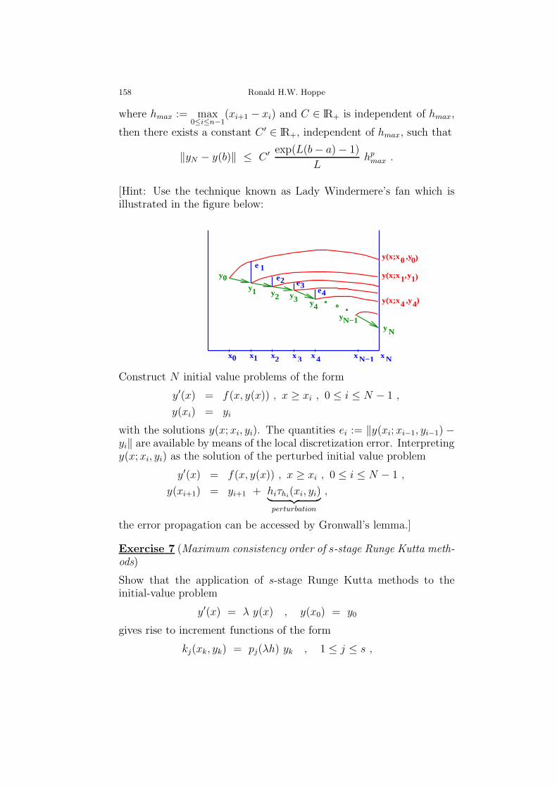
158 Ronald H.W. Hoppe
where hmax := max0≤i≤n−1
(xi+1 − xi) and C ∈ lR+ is independent of hmax,
then there exists a constant C ′ ∈ lR+, independent of hmax, such that
‖yN − y(b)‖ ≤ C ′ exp(L(b− a)− 1)
Lhpmax .
[Hint: Use the technique known as Lady Windermere’s fan which isillustrated in the figure below:
2e1e
Ny
e
N−1
43y 4e
3
y
yy
y0y
1
y,y(x;x
)0,y0
)
)4 4,yy(x;x
1 1
y(x;x
3xxx0x
2
1 NxN−1x4x2
Construct N initial value problems of the form
y′(x) = f(x, y(x)) , x ≥ xi , 0 ≤ i ≤ N − 1 ,
y(xi) = yi
with the solutions y(x; xi, yi). The quantities ei := ‖y(xi; xi−1, yi−1)−yi‖ are available by means of the local discretization error. Interpretingy(x; xi, yi) as the solution of the perturbed initial value problem
y′(x) = f(x, y(x)) , x ≥ xi , 0 ≤ i ≤ N − 1 ,
y(xi+1) = yi+1 + hiτhi(xi, yi)
︸ ︷︷ ︸
perturbation
,
the error propagation can be accessed by Gronwall’s lemma.]
Exercise 7 (Maximum consistency order of s-stage Runge Kutta meth-ods)
Show that the application of s-stage Runge Kutta methods to theinitial-value problem
y′(x) = λ y(x) , y(x0) = y0
gives rise to increment functions of the form
kj(xk, yk) = pj(λh) yk , 1 ≤ j ≤ s ,

Numerical Differential Equations 159
where pj are polynomials of degree at most j. Use this result for the de-termination of the maximum consistency order of s-stage Runge Kuttamethods.
Exercise 8 (Runge Kutta methods without memory)
(i) Compute all Runge Kutta methods of order 2 having the Butcherscheme
c1 = 0c2 c2c3 0 c3
0 0 1
(ii) In algorithmic notation derive an efficient implementation withrespect to storage.
(iii) Compute the polynomials pj , 1 ≤ j ≤ 3, as introduced in Exercise7.
Exercise 9 (Asymptotic expansion for the explicit Euler method)
Gragg’s theorem tells us that the coefficients in the asymptotic expan-sion of the global discretization error are solutions of inhomogeneouslinear initial-value problems. These initial-value problems should bederived for a specific problem: The discretization of the initial-valueproblem y′(x) = y(x) , y(a) = α by the explicit Euler scheme withconstant step size h gives rise to the difference equation
yh(x+ h) = yh(x) + h yh(x) , yh(a) = α .
Consider the asymptotic expansion
yh(x) =∞∑
k=0
ek(x) hk
and compute the staggered system of differential equations for the de-termination of the coefficients ek, k ∈ lN0, as well as the initial condi-tions. Compute e0 and e1 explicitly.
Exercise 10 (Consistency of linear multi-step methods)
Assume f ∈ Cp(I×D), I := [a, b] ⊂ lR, D ⊂ lRd and α ∈ lRd. Considerthe initial-value problem
(IV P1) y′(x) = f(x, y(x)) , x ∈ I ,
(IV P2) y(a) = α .
For a given equidistant partition xj := a+ jh, h := (b− a)/N,N ∈ lN,of I and given real numbers αk, βk, 0 ≤ k ≤ m,m ∈ lN, with αm 6= 0
160 Ronald H.W. Hoppe
and vectors α(j) ∈ lRd, 0 ≤ j ≤ m− 1, a linear multi-step method is ofthe form
(MSM1)1
h
m∑
k=0
αk yj+k =
m∑
k=0
βk f(xj+k, yj+k) , 0 ≤ j ≤ N −m ,
(MSM2) yj = α(j) , 0 ≤ j ≤ m− 1 .
Denoting by τh the local discretization error, suppose that
(⋆) τh(xj) = O(hp) , 0 ≤ j ≤ m− 1 .
Show that the linear multi-step method (MSM)1, (MSM)2 is consis-tent with the initial-value problem (IV P )1, (IV P )2 of order p if andonly if it is consistent of order p with
(IV P′
1) y′(x) = y(x) , x ∈ I ,
(IV P′
2) y(a) = 1 .
Exercise 11 (Stability of multi-step methods)
In class, the stability of multi-step methods has been investigated bymeans of the Lipschitz stability of operators on the linear space of gridfunctions. This approach can be generalized as follows:Let (X, ‖·‖X) and (Y, ‖·‖Y ) be normed spaces and let (Ah)h be a familyof continuous operators Ah : X → Y . This family is called Lipschitzstable, if there exist positive numbers δ, η such that for all x, z ∈ Xand all h satisfying
(LS)1 ‖Ahx−Ahz‖Y ≤ δ
there holds
(LS)2 ‖x− z‖X ≤ η ‖Ahx− Ahz‖Y .
(i) For Lipschitz stable families of continuous linear operators Ah :X → Y derive a simpler definition of stability by taking advantage ofthe linearity.
(ii) Let (Ah)h be a Lipschitz stable family of continuous linear opera-tors which are additionally assumed to be surjective.Show that for all h the operatorAh is invertible with ‖A−1
h ‖ ≤ C,C > 0,and derive an upper bound for the constant C.(Hint: Show injectivity first and then use the definition of the operator
norm ‖Ah‖ = sup06=x∈X
‖Ahx‖Y‖x‖X
.)
(iii) Let H be a Hilbert space, i.e., a complete inner product spacewith inner product < ·, · >: H ×H → lR, and let (Ah)h be a family of

Numerical Differential Equations 161
continuous endomorphisms Ah : H → H . Further, let ah : H×H → lRbe the bilinear form given by ah(x, y) :=< Ahx, y >.Prove the equivalence of the following two statements:
(∗) For all h the operator Ah is invertible such that ‖A−1h ‖ ≤ C, where
C is a positive constant independent of h.
(∗∗) There holds
sup‖y‖=1
|ah(x, y)| >1
C‖x‖ , x ∈ H ,
sup‖x‖=1
|ah(x, y)| > 0 , 0 6= y ∈ H .
(Hint: For (∗) =⇒ (∗∗) use ‖x‖ = sup< x, y > | ‖y‖ = 1, x ∈ H .For (∗∗) =⇒ (∗) verify first that ‖Ahx‖ ≥ C−1‖x‖, x ∈ H . Then, usingan arbitrary Cauchy sequence, show that the range of each operatorAh is closed. Finally, prove surjectivity by contradiction, i.e., assumerange(Ah)
⊥ 6= 0.)
Exercise 12 (Affine-Invariance of Runge-Kutta methods)
Consider the initial-value problem
(∗) y′(x) = f(x, y(x)) , y(a) = α ,
where f : lR× lRm → lRm, a ∈ lR and α ∈ lRm. After a transformationy = Ay with a regular matrix A ∈ lRm×m the initial-value takes theform
(∗∗) y′(x) = A f(x,A−1y(x)) , y(a) = A α .
Show that any Runge-Kutta method inherits this property, i.e., it isaffine invariant in the following sense: If the application of the RungeKutta method to (∗) results in a grid function yk, k ∈ lN0,, then theapplication of the method to (∗∗) results in the grid function Ayk, k ∈lN0.
Exercise 13 (Maximal Consistency Order of s-Stage Runge Kutta Meth-ods)
Show that the application of an s-stage Runge Kutta method to theinitial-value problem
y′(x) = λ y(x) , y(x0) = y0
yields increment functions of the form
kj(xk, yk) = pj(λh) yk , 1 ≤ j ≤ s ,
162 Ronald H.W. Hoppe
where pj are polynomials of degree at most j. Use this result to deter-mine the maximal consistency order of s-stage Runge Kutta methods.
Exercise 14 (Cauchy’s θ-Method)
Consider the initial-value problem
(∗) y′(x) = f(x, y(x)) , x ≥ a , y(a) = α ,
where f : lR× lRm → lRm and α ∈ lRm.Show that the only consistent linear one-step method for the numericalsolution of (∗) are given by the one-parameter family
yh(xk+1) = yh(xk) + h((1− θ)f(xk, yh(xk)) + θf(xk+1, yh(xk+1))
).
(i) Which values of θ ∈ lR provide the consistency order p = 2?
(ii) Which methods result for θ = 0, θ = 0.5, and θ = 1.0?
Exercise 15 (Runge Kutta Fehlberg 1(2) Method)
Consider the initial-value problem
y′(x) = f(x, y(x)) , y(a) = α.
For the numerical solution use Runge Kutta methods of order 1 and 2
yh(a + h) = yh(a) + h (b1 k1 + b2 k2 ) ,(2.156)
y(a+ h) − yh(a+ h) = O(h2)(2.157)
yh(a+ h) = yh(a) + h ( b1 k1 + b2 k2 + b3 k3 ) ,(2.158)
y(a+ h) − yh(a + h) = O(h3)(2.159)
with step size h and the increments
k1 = f(a, α) ,
ki = f(a + ci h, α + h
i−1∑
j=1
aij kj) , 2 ≤ i ≤ 3 .
(i) Derive order conditions for the coefficients ci, aij , bi and bi. Observethat here ci =
∑
j aij is not requested.
(ii) How many function evaluations per step are required by (2.156),(2.157)and (2.158),(2.159)?
(iii) The embedded method uses Fehlberg’s trick in the sense that yhis used in the following step: One takes advantage in the choice of theparameters to use the increment k3 as the increment k1 in the following

Numerical Differential Equations 163
step which results in a reduction of the computational work. Deriveconditions for the coefficients ci, a31, and a32 such that the applicabilityof Fehlberg’s trick is guaranteed.
(iv) Consider the local discretization error of the method (2.158),(2.159)
including Fehlberg’s trick from (iii) and the simplification b2 = b2.Compute the coefficient of the lowest power in h. What are the conse-quences of the choice c2 =
12, b2 = 1 taking into account that embedded
methods are used for step size control?
(v) The potential advantages of RKF-1(2) methods are not completelyexhausted by Fehlberg’s trick: Compute the parameters such that aRunge Kutta Fehlberg method of order 1 is obtained which only re-quires one function evaluation per step.
(vi) Sketch the method from (v) in algorithmic notation with thefollowing step size control: an integration step has to be repeated withthe computed smaller step size, if the estimated error EST exceeds auser specific tolerance TOL. Otherwise, the following integration stepis performed with the suggested step size. In order to prevent largeoscillations in the step size use
hnew := hmin(facmax, max(facmin, fac(TOL/EST )1/(p+1)))
with a safety factor fac := 0.9 and the limiters
facmin := 0.5 , facmax := 2.0 .
Exercise 16 (BDF)
BDF rely on the idea to compute the approximation yj+m in xj+m asthe value of the interpolating polynomial p ∈ Pm with
p(xℓ) = yℓ , j ≤ ℓ ≤ j +m− 1 ,
p′(xj+m) = f(xj+m, yj+m) ,
i.e., the polynomial interpolates the previously computed approxima-tions in xj , ..., xj+m−1 and solves the differential equation in xj+m.
(i) Show that for constant step size h := xk+1 − xk BDF is a linearm-step method of the form
1
h
m∑
k=0
αk yj+k =
m∑
k=0
βk f(xj+k, yj+k) , 0 ≤ j ≤ N .
Compute the coefficients αk , βk from the Lagrange fundamental poly-nomials Li ∈ Pm with Li(xj+k) = δik , 0 ≤ i, k ≤ m.

164 Ronald H.W. Hoppe
(ii) Derive a representation of BDF on the basis of Newton’s represen-tation of the interpolating polynomials. In particular, show: If
∇0fj := fj , 0 ≤ j ≤ m ,
∇pfj := ∇p−1fj − ∇p−1fj−1 , p ≤ j ≤ m , 1 ≤ p ≤ m
are the backward differences with respect to the nodes (xj , yj) , 0 ≤j ≤ m, where xj = x0 + jh , 0 ≤ j ≤ m, then the interpolatingpolynomial pq ∈ Pq with pq(xj) = fj , m− q ≤ j ≤ m, is given by
pq(x) =
q∑
j=0
(−1)j (−sj ) ∇jfm .
Here s := (x− xm)/h.
(iii) In addition to part (ii) show that implicit BDF with constant stepsize h have the equivalent representation
m∑
k=1
1
kyj+m = f(xj+m, yj+m) .
(iv) For an equidistant grid of step size h give an explicit representationof BDF with m = 3.
(v) Using the representation in (i) and
τh(x) =1
h
m∑
k=0
αk y(x − (m− k) h) −m∑
k=0
βk y′(x − (m− k) h) ,
compute the local discretization error.
(vi) Compute the order of consistency.
Exercise 17 (Stability of BDF)
Dahlquist has shown that there are no A-stable linear multi-step meth-ods of order > 2. On the other hand, an m-step BDF has the orderof consistency m. Hence, for m ≥ 3 BDF can not be A-stable. In tisexercise we prove this fact based on the definition of stability.
(i) Derive the formulas for BDF with m = 2 andm = 3 in the standardrepresentation of linear multi-step methods.(Hint: Use the representation from Exercise 16 (i).)
(ii) Show that BDF with m = 2 is A-stable, but not the one withm = 3.(Hint: Use Dahlquist’s root condition.)

Numerical Differential Equations 165
Exercise 18 (Adams-Bashforth Method)
Consider the scalar initial-value problem
y′(x) = f(x, y(x)) , y(a) = α .
Show that the Adams-Bashforth m-step method has the representation
yj+m = yj+m−1 +
xj+m∫
xj+m−1
p(x) dx ,
where p ∈ Pm−1 is the polynomial with p(xk) = f(xk, yk), j ≤ k ≤j+m−1. In the sequel assume an equidistant grid of step size h > 0.
(i) Prove the stability of the m-step Adams-Bashforth method.
(ii) Compute the consistency of the m-step Adams-Bashforth method.
(iii) Using part (ii) of Exercise 16 prove the following representationof the m-step Adams-Bashforth method on the basis of backward dif-ferences
yj+m = yj+m−1 + h
m−1∑
k=0
γk ∇kfj+m−1 , 0 ≤ j ≤ N −m ,
where
γk = (−1)k1∫
0
(−sk ) ds .
(iv) Prove the following property of the coefficients γk of part (iii)
k∑
ℓ=0
1
k − ℓ + 1γℓ = 1 .
(Hint: Consider a power series with coefficients γk and use the Cauchyproduct of power series.)
Exercise 19 (Stability of semi-implicit methods)
Solve the stiff, autonomous, scalar initial value problem
y′(x) = f(y(x)) , y(a) = α
by means of a semi-implicit numerical integrator using a single Newtonstep for the nonlinear equation which determines the approximationyk+1. As initial guess choose the approximation yk known from theprevious step.

166 Ronald H.W. Hoppe
(i) A simplified version of the semi-implicit Euler method is given bythe difference equation
yk+1 = yk + (1 − h a)−1 h f(yk) , k ∈ lN0
with a suitable approximation a of the derivative fy. Apply the methodto the test problem
(⋆) y′ = λ y , y(0) = 1 (λ ∈ C , Reλ < 0)
and set z := λh , z0 := ah, where z0 is supposed to have a negativereal. Prove the A-stability of the method for z = z0.
(ii) For z 6= z0, compute the boundary ∂G of the stability region
G(z0) := z ∈ C | |R(z, z0)| ≤ 1(R denotes the stability function). For z0 = −1 + i, display ∂G in thecomplex plane.
(iii) Apply the semi-implicit midpoint rule (without initial and finalstep)
yk+1 = (1 − ha)−1 ((1 + ha) yk−1 + 2 h f(yk))
to the scalar test equation (⋆) and use z , z0 as in part (i). Verify theA-stability for z = z0.
(iv) For z 6= z0, use the ansatz yk = ξk to derive the associatedcharacteristic polynomial. Denote by ξ1(z, z0) and ξ2(z, z0) the zeroesof this polynomial. Determine the boundary ∂G of the stability region
G(z0) := z ∈ C | |ξi(z, z0)| ≤ 1 , 1 ≤ i ≤ 2and study the special case z0 ∈ lR.
Exercise 20 (Method of lines)
The spatial and temporal distribution of the temperature u(x, t) in ahomogeneous slab of length 1m the endpoints of which are kept at theconstant temperature 00C can be described by the heat equation
∂u
∂t(x, t) =
∂2u
∂x2(x, t) , (x, t) ∈ lR+ × (0, 1) ,
u(x, 0) = u0(x) , x ∈ (0, 1) ,
u(0, t) = u(1, t) = 0 , t ∈ lR+ ,
where u0(0) = u0(1) = 0.Discretize in space by means of symmetric difference quotients withrespect to an equidistant grid (xi)
ni=0 , xi := ih , 0 ≤ i ≤ n , h := 1/n:
∂2u
∂x2(xi, t) ≈ u(xi + h, t)) − 2u(xi, t) + u(xi − h, t)
h2.

Numerical Differential Equations 167
This leads to a system of first order ordinary differential equations forthe time-dependent grid function (ui(t))
n−1i=1 with ui(t) ≈ u(xi, t) , 1 ≤
i ≤ n− 1, where u0 = un = 0. The initial values are given by ui(0) :=u0(xi).
(i) Derive the resulting initial value problem for a linear autonomoussystem of the form
u′(t) = Au(t) ,
where A ∈ lR(n−1)×(n−1) and u(t) := (ui(t))n−1i=1 ∈ lRn−1.
(ii) Show that the grid functions ek := (sinhπik)n−1i=1 , 1 ≤ k ≤ n− 1,
form an orthonormal system of eigenvectors of A from part (i).
(iii) Why is the system of ordinary differential equations a stiff system?
(iv) Use an algorithmic notation to formulate an efficient procedurefor the simulation of the temperature distribution in the slab wherethe granularity h of the discretization in space and the step size ∆t intime are the input parameters.
Exercise 21 (Stability of extrapolation methods)
Extrapolation techniques can also be used for stiff methods to constructnumerical integrators of higher order. However, the stability propertyof the basis scheme are not automatically inherited by the resultingmethod.
(i) Prove the A-stability of the implicit trapezoidal rule
yk+1 = yk +h
2(f(xk, yk) + f(xk+1, yk+1)) .
(ii) It is well-known that the implicit trapezoidal rule admits an h2-expansion of the global discretization error. Extrapolate by means ofn1 = 1 and n2 = 2 (number of micro steps) and show that A-stabilitygets lost for the resulting scheme.
(iii) Now, extrapolate with n1 = 2, n2 = 4 and show that the applica-tion to the scalar test equation y′ = λy, λ ∈ C, gives rise to a stabilityfunction R22 of the resulting scheme with the property
limz→−∞
|R22(z)| = 1 , z := λh .
(iv) Prove that the scheme from part (iii) is not A-stable no matterhow n1, n2 are chosen.
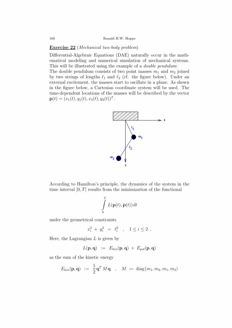
168 Ronald H.W. Hoppe
Exercise 22 (Mechanical two-body problem)
Differential-Algebraic Equations (DAE) naturally occur in the math-ematical modeling and numerical simulation of mechanical systems.This will be illustrated using the example of a double pendulum:The double pendulum consists of two point masses m1 and m2 joinedby two strings of lengths ℓ1 and ℓ2 (cf. the figure below). Under anexternal excitement, the masses start to oscillate in a plane. As shownin the figure below, a Cartesian coordinate system will be used. Thetime-dependent locations of the masses will be described by the vectorp(t) = (x1(t), y1(t), x2(t), y2(t))
T .
l
m1
1
2
2m
l
y
x
According to Hamilton’s principle, the dynamics of the system in thetime interval [0, T ] results from the minimization of the functional
T∫
0
L(p(t), p(t))dt
under the geometrical constraints
x2i + y2i = ℓ2i , 1 ≤ i ≤ 2 .
Here, the Lagrangian L is given by
L(p,q) := Ekin(p,q) + Epot(p,q)
as the sum of the kinetic energy
Ekin(p,q) :=1
2qT M q , M := diag(m1, m2, m1, m2)

Numerical Differential Equations 169
and the potential energy
Epot(p,q) := −g (m1 y1 + m2 y2 ) ,
where g denotes the gravitational constant.
(i) Derive the saddle point problem which results by coupling the
constraints using a Lagrangian multiplier ~λ ∈ R2.
(ii) Derive the necessary optimality conditions in case of a sufficientlysmooth trajectory p (Euler-Lagrange equations).
(iii) Rewrite the Euler-Lagrange equations for the double pendulumand the geometrical constraints as a differential-algebraic system.
(iv) Compute the index of the DAE from part (iii).
Exercise 23 (Laplace operator in polar coordinates)
Consider the Laplace operator
∆ =∂2
∂x21+
∂2
∂x22
and show that in polar coordinates (r, ϕ) it is given by
∆ =∂2
∂r2+
1
r
∂
∂r+
1
r2∂2
∂ϕ2.
Exercise 24 (Solution of an elliptic boundary value problem)
Let Ω ⊂ lR2 be the domain given by
Ω := (r, ϕ) | 0 ≤ r < 1, 0 < ϕ <7
4π
with boundary Γ = Γ1 ∪ Γ2 ∪ Γ3, where
Γ1 := (r, 0) | 0 < r < 1,
Γ2 := (r, 74π) | 0 < r < 1,
Γ3 := (1, ϕ) | 0 < ϕ <7
4π.
Show that the solution of the elliptic boundary value problem
−∆u = 0 in Ω,
u = 0 on Γ1 ∪ Γ2,
u = sin(4
7π) on Γ3
is given by u(r, ϕ) = r4/7 sin(47π).
170 Ronald H.W. Hoppe
Exercise 25 (Fundamental solution)
Let Bd1 be the unit ball in lRd, d ≥ 2, and let |Bd
1 | be its volume. Showthat the function
Γ(x, y) :=
12π
ln(|x− y|), d = 21
d(2−d)|Bd1 |
|x− y|2−d, d > 2 ,
considered as a function of x, is a harmonic function in lRd \ y.
Exercise 26 (Nine point approximation of the Laplace operator)
For a sufficiently smooth function u show that the nine point formula
1
h2
(8
3u(x, y)− 1
3(u(x, y − h) + u(x− h, y) + u(x+ h, y) + u(x, y + h))
−1
3(u(x− h, y − h) + u(x+ h, y − h) + u(x− h, y + h) + u(x+ h, y + h))
)
provides an approximation of −∆u of order O(h2).
Exercise 27 (Checkerboard ordering of grid points)
Let Ω = (a, b)2, a, b ∈ lR, a < b, and let Ωh be a uniform grid of stepsize h = (b − a)/(N + 1), N ∈ lN. For the numerical solution of thePoisson equation with homogeneous Dirichlet boundary conditions
−∆u = f in Ω,
u = 0 on Γ
use the five point approximation of the Laplace operator. Determinethe block structure of the coefficient matrix Ah of the resulting linearalgebraic system
Ahuh = bhfor a checkerboard ordering of the grid points.
Exercise 28 (Eigenvalues and eigenfunctions of the discrete Laplaceoperator)
Let Ω = (a, b)2, a, b ∈ lR, a < b, and let Ωh be a uniform grid with stepsize h = (b − a)/(N + 1), N ∈ lN. For the numerical solution of thePoisson equation with homogeneous Dirichlet boundary conditions
−∆u = f in Ω,
u = 0 on Γ
use the five point approximation of the Laplace operator. Show thatthe coefficient matrix Ah of the resulting linear algebraic system
Ahuh = bh

Numerical Differential Equations 171
has the eigenvalues
λij = 4h−2(
sin2(iπh/2) + sin2(jπh/2))
, 1 ≤ i, j ≤ N,
and the associated eigenfunctions x(ij) ∈ lRN2
according to
x(ij)kℓ =
h
2sin(ihkπ) sin(jhℓπ), 1 ≤ k, ℓ ≤ N.
Compute the spectral condition Ah. How does the spectral conditionbehave N → ∞?
Exercise 29 (Non-smooth solution)
Let Ω ⊂ lR2 be the domain given by
Ω := (r, ϕ) | 0 ≤ r < 1, 0 < ϕ <7
4π
with boundary Γ = Γ1 ∪ Γ2 ∪ Γ3, where
Γ1 := (r, 0) | 0 < r < 1,
Γ2 := (r, 74π) | 0 < r < 1,
Γ3 := (1, ϕ) | 0 < ϕ <7
4π.
The solution of the elliptic boundary value problem
−∆u = 0 in Ω,
u = 0 on Γ1 ∪ Γ2,
u = sin(4
7π) on Γ3
is given by u(r, ϕ) = r4/7 sin(47π).
Show that u ∈ H1(Ω), but u /∈ H2(Ω).
Exercise 30 (Poincare-Friedrichs inequality)
Let Ω ⊂ lRd be a bounded domain with boundary Γ = ∂Ω. For u ∈H1
0 (Ω) the Poincare-Friedrichs inequality∫
Ω
|u|2 dx ≤ CΩ
∫
Ω
|∇u|2 dx
holds true with a constantCΩ > 0. Show that CΩ ≥ 1/λ1, where λ1 isthe smallest eigenvalue of the eigenvalue problem
−∆u = λu in Ω, u = 0 on Γ.

172 Ronald H.W. Hoppe
Exercise 31 (Robin boundary condition)
Let Ω ⊂ lRd be a bounded domain with boundary Γ = ∂Ω, f ∈ L2(Ω),g ∈ L2(Γ), and r ∈ L∞(Γ) with r(x) ≥ r0 > 0 for almost all x ∈ Γ.Consider the Poisson equation with Robin boundary conditions
−∆u = f in Ω,
ν · ∇u+ ru = g on Γ,
where ν is the outward unit normal vector on Γ.Show that the weak solution of the boundary value problem satisfiesthe variational equation∫
Ω
∇u · ∇v dx+∫
Γ
ruv dσ =
∫
Ω
fv dx+
∫
Γ
gv dσ, v ∈ H1(Ω),
and prove existence and uniqueness of a weak solution.
Exercise 32 (Representation of nodal basis functions)
Let T be a non-degenerate triangle in lR2 with vertices ai and edgesEi, 1 ≤ i ≤ 3, where the edge Ei is opposite to the vertex ai. Further,let mEi
and νEibe the midpoints and outward unit normal vectors of
the edges. Show that the nodal basis functions ϕi of the finite elementspace of simplicial Lagrangean finite elements of type (1) have therepresentation
ϕi(x) = − |Ei|2|T | νEi
· (x−mEi) , 1 ≤ i ≤ 3,
where |Ei| is the length of Ei and |T | is the area of T .
Exercise 33 (Representation of the local stiffness matrix)
Let T be a non-degenerate triangle in lR2 of area |T | with the verticesai , 1 ≤ i ≤ 3, and the edges Ei of length |Ei| opposite of ai. Further,let αij , 1 ≤ i < j ≤ 3, be the interior angles formed by the edgesEi and Ej and let ϕi , 1 ≤ i ≤ 3, be the nodal basis functions of thefinite element space of simplicial Lagrangean finite elements of type(1). Show that the local stiffness matrix S ∈ lR3×3 with the elementsSij =
∫
T
∇ϕi · ∇ϕjdx , 1 ≤ i, j ≤ 3, is given by
S =1
4|T |
|E1|2 −cot(α12) −cot(α13)−cot(α12) |e2|2 −cot(α23)−cot(α13) −cot(α23) |E3|2
.
Numerical Differential Equations 173
Exercise 34 (Quadratic Lagrangean finite elements)
For the numerical solution of the elliptic boundary value problem
−∆u(x) = 0 x = (x1, x2)T ∈ Ω := (0, 1)2 ,
u(x) = x21 + x22 on Γ := ∂Ω
use a finite element discretization by simplicial Lagrangean finite el-ements of type (2) with respect to a uniform simplicial triangulationTh(Ω) which is generated as follows: Use a partition of Ω into a qua-dratic grid of step size h = 1/(N + 1), N ∈ lN, and subdivide eachcell into two triangles by the diagonal from bottom left to top right.Use the canonical nodal basis functions with respect to a lexicographicordering of the grid points.
(i) For the reference triangle T with vertices a1 = (0, 0), a2 = (1, 0),and a3 = (0, 1) compute the nodal basis functions ϕai , 1 ≤ i ≤ 3, andϕaij , aij := (ai + aj)/2, 1 ≤ i < j ≤ 3, as functions of x = (x1, x2) andcompute their gradients.
(ii) For an actual triangle T ∈ Th(Ω) of area |T | compute the localstiffness matrix using the quadrature formula
∫
T
f(x) dx ≈ 1
3|T |
∑
1≤i<j≤3
f(aij) .
How big is the quadrature error?
(iii) For h = 1/3 sketch the triangulation, mark the nodal points by×, and order them according to the lexicographic ordering.
(iv) For h = 1/3 sketch the sparsity pattern of the global stiffnessmatrix.
Exercise 35 (Method of alternating directions I)
For the numerical solution of the heat equation
∂u
∂t− ∆u = f
in Q := Ω × (0, T ),Ω = (a, b)2 ⊂ lR2, use uniform partitions tm =mτ, 0 ≤ m ≤ M of [0, T ] of step size τ = T/M,M ∈ lN, and(xi, yj) | xi = a + ih, yj = a + jh, 1 ≤ i, j ≤ N + 1 of Ω ofstep size h = (b − a)/(N + 1), N ∈ lN. Let Um
ij , 0 ≤ m ≤ M, and
Um+1/2ij , 0 ≤ m ≤ M − 1, be approximations of u(xi, yj, tm) resp.
u(xi, yj, tm + τ/2). Show that for sufficiently smooth u the method
174 Ronald H.W. Hoppe
of alternating directions
Um+1/2ij − Um
ij
τ/2− U
m+1/2i−1,j − 2U
m+1/2ij + U
m+1/2i+1,j
h2
−Umi,j−1 − 2Um
ij + Umi,j+1
h2= f
m+1/2ij ,
Um+1ij − U
m+1/2ij
τ/2− U
m+1/2i−1,j − 2U
m+1/2ij + U
m+1/2i+1,j
h2
−Um+1i,j−1 − 2Um+1
ij + Um+1i,j+1
h2= f
m+1/2ij ,
has the consistency order 2 in space and time.What is the advantage of the method with regard to the numericalsolution of the resulting linear algebraic system?
Exercise 36 (Method of alternating directions II)
Consider the heat equation from Exercise 35 with the boundary con-dition
u = uD on Σ := ∂Ω × (0, T ]
and the initial condition
u(·, 0) = u0 in Ω.
Apply the method of alternating directions from Exercise 35 and set
Um+1/2j := (Um+/2
1j , Um+1/22j , · · · , Um+1/2
Nj )T , 1 ≤ j ≤ N.
Show that for each j one has to solve a linear algebraic system
AUm+1/2j = b
with a symmetric tridiagonal matrix A ∈ lRN×N and a vector b ∈ lRN .Compute A and b explicitly.