Appl. Comput. Harmon. Anal. 29 (2010) 2–17

Contents lists available at ScienceDirect

Applied and Computational Harmonic Analysis

www.elsevier.com/locate/acha

Numerical computation of complex geometrical optics solutions to theconductivity equation

Kari Astala a, Jennifer L. Mueller b, Lassi Päivärinta a, Samuli Siltanen a,∗a Department of Mathematics and Statistics, University of Helsinki, Finlandb Department of Mathematics and School of Biomedical Engineering, Colorado State University, USA

a r t i c l e i n f o a b s t r a c t

Article history:Received 6 November 2008Revised 30 July 2009Accepted 5 August 2009Available online 8 August 2009Communicated by Wolfgang Dahmen

Keywords:Inverse problemBeltrami equationNumerical solverConductivity equationInverse conductivity problemQuasiconformal mapComplex geometrical optics solutionNonlinear Fourier transformElectrical impedance tomography

A numerical method is introduced for the evaluation of complex geometrical optics (cgo)solutions to the conductivity equation ∇ · σ∇u(·,k) = 0 in R

2 for piecewise smoothconductivities σ . Here k is a complex parameter. The algorithm is based on the solution byAstala and Päivärinta (2006) [1] of Calderón’s inverse conductivity problem and involvesthe solution of a Beltrami equation in the plane with an exponential asymptotic condition.The numerical strategy is to solve a related periodic problem using fft and gmres andshow that the solutions agree on the unit disc. The cgo solver is applied to the problem ofcomputing nonlinear Fourier transforms corresponding to nonsmooth conductivities. Thesecomputations give new insight into the D-bar method for the medical imaging technique ofelectric impedance tomography. Furthermore, the asymptotic behavior of the cgo solutionsas k → ∞ is studied numerically. The evidence so gained raises interesting questions aboutthe best possible decay rates for the subexponential growth argument in the uniquenessproof for Calderón’s problem with L∞ conductivities.

© 2009 Elsevier Inc. All rights reserved.

1. Introduction

We consider the numerical evaluation of complex geometrical optics (cgo) solutions to the conductivity equation

∇ · σ∇uσ = 0 in R2, (1.1)

for piecewise smooth conductivities σ . We assume that σ is measurable and bounded away from 0 and infinity, withσ(x) ≡ 1 for x outside a compact set. The cgo solutions are specified by their asymptotics

uσ (z,k) = eikz(

1 + O(

1

z

)), as |z| → ∞, (1.2)

where k ∈ C is a parameter. The solutions play a key role in solving the fundamental Calderón problem [1–3,17–19,21],which we next describe in detail.

* Corresponding author.E-mail address: samuli.siltanen@iki.fi (S. Siltanen).

1063-5203/$ – see front matter © 2009 Elsevier Inc. All rights reserved.doi:10.1016/j.acha.2009.08.001

K. Astala et al. / Appl. Comput. Harmon. Anal. 29 (2010) 2–17 3

Suppose that Ω ⊂ R2 is the unit disc and σ : Ω → (0,∞) is measurable and satisfies 0 < c � σ(z) < ∞ almost every-

where. Let u ∈ H1(Ω) be the unique solution to

∇ · σ∇u = 0 in Ω, (1.3)

u|∂Ω = f ∈ H1/2(∂Ω). (1.4)

Static voltage-to-current measurements at the boundary can be modeled by the Dirichlet-to-Neumann map

Λσ : H1/2(∂Ω) → H−1/2(∂Ω), f → σ∂u

∂n

∣∣∣∣∂Ω

.

Calderón posed the question in [3] whether σ is uniquely determined by Λσ , and if so, how to reconstruct σ when Λσ

is given. This problem is also known as electrical impedance tomography (eit), an imaging technique with applications inmedicine, geophysics, and industrial process monitoring [4].

In dimension 2, Calderón’s problem was recently solved using cgo solutions by Astala and Päivärinta [1]. In the case ofL∞-conductivities the cgo solutions need to be constructed via the Beltrami equation

∂ z fμ = μ∂z fμ, (1.5)

where μ is a compactly supported L∞ function, connected to σ by the identity

μ := 1 − σ

1 + σ. (1.6)

Here z = z1 + iz2 ∈ C and ∂ z = (∂/∂z1 + i∂/∂z2)/2. Indeed, the respective complex geometric optics solutions are related bythe equation

2uσ (z,k) = fμ(z,k) + f−μ(z,k) + fμ(z,k) − f−μ(z,k). (1.7)

The simple reason behind these identities is that the real part u of fμ(z,k) solves Eq. (1.1) while the imaginary part solvesthe same equation with σ replaced by 1/σ .

An asymptotic condition similar to (1.2) is required:

fμ(z,k) = eikz(1 + ω(z,k))

with ω(z,k) = O(

1

z

)as |z| → ∞. (1.8)

In particular, constructing solutions to (1.1) is now reduced to considering the Beltrami equation (1.5).In this paper we introduce a numerical algorithm for the computation of the cgo solutions fμ of the form (1.8), satis-

fying the Beltrami equation (1.5) for a given μ = (1 − σ)/(1 + σ). Simultaneously we obtain the cgo solutions uσ for theconductivity equation (1.1). We assume that σ is piecewise continuous in the following sense.

Definition 1. We say that σ is piecewise continuous if σ ∈ C0(Ω \Γ ), where Γ is the union of a finite number of piecewiseC1 curves Γi : [0,1] → Ω for which Γi ∩ Γ j is a discrete set whenever i �= j.

This is a reasonable assumption for medically relevant conductivities. The algorithm is based on periodization, truncationof a Neumann series, discretization, and the use of fast Fourier transform and the iterative gmres solver. The basic ideas forthe numerical part of this work come from Vainikko’s solution method [22] for the Lippmann–Schwinger equation, and fromthe generalization of that method for the ∂ equation by Knudsen, Mueller and Siltanen [14]. We remark that the presentgeneralization of [22] is more complicated than the one reported in [14].

Numerical computation of solutions to the Beltrami equation have been described in [5,8]. Those two approaches do notapply to the exponential asymptotic condition (1.8) of interest here.

We verify our new algorithm by comparison to Faddeev’s cgo solutions for the Schrödinger equation [7]. Those solu-tions are used in Nachman’s uniqueness proof [17] for Calderón’s problem assuming twice differentiable conductivities.The numerical computation of these solutions, henceforth called the benchmark method, is already well understood [15,19].Eq. (1.7) leads to a simple formula connecting the two cgo solutions when the conductivity is smooth, and we can checkthat the two algorithms agree. In fact, for k close to zero the new algorithm is found to give more accurate results than thebenchmark method.

Applications of our new algorithm include

(i) Checking intermediate results when developing eit algorithms based on [1],(ii) Evaluating Faddeev’s cgo solutions accurately for k near zero,

(iii) Computing nonlinear Fourier transforms numerically,(iv) Studying quasiconformal mappings.

4 K. Astala et al. / Appl. Comput. Harmon. Anal. 29 (2010) 2–17

Goal (i) is a large project of its own and will not be discussed further here. Concerning (iii), we compute for the first timethe scattering transform (also called the nonlinear Fourier transform) t : C → C corresponding to a discontinuous conduc-tivity. For this, we provide new insight by numerical experiments. Our results suggest that for nonsmooth conductivitiesthere may not exist large |k| estimates of the form |t(k)| � C |k|λ with λ � 0. Note that in the smooth case it is known[19, Theorem 3.2] that |t(k)| � |k|−m for large |k| if σ ∈ C2+m(Ω) and m � 1. Approximate scattering transforms for discon-tinuous conductivities were studied in [13].

As a contribution to (iv) we study numerically the behavior of fμ(·,k) when |k| grows. It was proven in [1] thatfμ(z,k) = exp(ikφμ(z,k)), where φμ is a quasiconformal homeomorphism satisfying φμ(z,k) = z + O(1/z) when z → ∞.The technically most demanding result in [1], crucially important for the uniqueness proof, is establishing the followingsubexponential growth result: limk→∞ φμ(z,k) = z uniformly in z ∈ C. Our computation yields numerical evidence for theexistence of an estimate of the form supz∈Ω |φμ(z,k) − z| � C |k|λ with λ < 0 in the case of simple piecewise smooth dis-continuous conductivity. This raises the very interesting question what are the best possible theoretical decay rates in thiscontext.

This paper is organized as follows. In Section 2 we derive a periodic construction of the cgo solutions fμ . The Neumannseries so achieved is truncated in Section 3 to give a numerically viable approximation to the cgo solutions, and in Sec-tion 4 we describe an algorithm for the evaluation of those approximations. In Section 5 we discuss cgo solutions for theSchrödinger equation, derive a connection between the two solution types, and verify the new cgo solver by comparison tothe benchmark method. In Section 6 we apply our method to the evaluation of nonlinear Fourier transforms correspondingto discontinuous conductivities. Section 7 is devoted to the numerical study of φμ(·,k) as k grows. Finally, in Section 8 wediscuss hardware issues and give directions for further study of efficiency and accuracy of our new method.

2. Construction of CGO solutions via periodization

The cgo solutions are constructed in [1] as follows. Define the solid Cauchy transform by

P f (z) = − 1

π

∫C

f (λ)

λ − zdm(λ), (2.1)

and Beurling transform by S f = ∂ P f . Note that P is the inverse operator of ∂ and that S transforms ∂ derivatives into ∂

derivatives: S(∂ f ) = ∂ f .Let Ω denote the unit disc. For given piecewise continuous conductivity σ : Ω → R and any complex number k ∈ C, set

μ = (1 − σ)/(1 + σ) and define

α(z,k) = −ike−k(z)μ(z), (2.2)

ν(z,k) = e−k(z)μ(z), (2.3)

where e−k(z) := exp(−i(kz + kz)). Then α(·,k), ν(·,k) ∈ L∞(Ω) and |ν(z,k)| = |μ(z,k)| � κ < 1 for almost every z. Thefollowing theorem was proven in [1].

Theorem 1 (Astala and Päivärinta). Let k ∈ C. Assume that α(·,k) ∈ L∞(Ω) and ν(·,k) ∈ L∞(Ω) and |ν(z,k)| � κ < 1 for almostevery z. Take 2 < p < 1 + 1/κ and define the operator K : L p(C) → L p(C) by

K g = P (I − νS)−1(αg). (2.4)

Then K : L p(C) → W 1,p(C) and I − K is invertible in L p(C). Further, equation

(I − K )ω = K (χΩ) (2.5)

has a unique solution with asymptotics ω(z,k) = O(1/z).

Let us recall the definition of the Sobolev space W 1,p(C):

W 1,p(C) ={

f ∈ Lp(C)

∣∣∣ ∂ f

∂z j∈ Lp(C) for j = 1,2

}.

We note that the Sobolev embedding theorem implies that W 1,p(C) functions are continuous when p > 2.The complex geometrical optics solutions fμ are given by substituting the unique solution of Eq. (2.5) to formula (1.8).

Next we derive a periodic equation equivalent to (2.5) and more suitable for numerical solution.According to [20] the Beurling transform S has the properties

S : Lr(C) −→ Lr(C), 1 < r < ∞, and ‖S‖L2−→L2 = 1. (2.6)

K. Astala et al. / Appl. Comput. Harmon. Anal. 29 (2010) 2–17 5

Thus ‖ν S̄‖L(L2(Q )) < 1, and consequently (I − νS)−1 can be expressed as a Neumann series. Denoting complex conjugation

as an operator ρ( f ) = f , we see that ω satisfies

∂ω = (I − νS)−1(αω + α) =∞∑

�=0

(νρ∂ P )�(αω + α). (2.7)

By the uniqueness result for Eq. (2.5), Eq. (2.7) has a unique solution with asymptotics ω(z,k) = O(1/z).Take ε > 0 and set s = 2 + 3ε . Define Q := [−s, s)2 and introduce a periodic version of Eq. (2.5) as follows. Choose an

infinitely smooth cutoff function η ∈ C∞0 (R2) satisfying

η(z) =⎧⎨⎩

1 for |z| < 2 + ε,

smooth for 2 + ε � |z| < 2 + 2ε,

0 for |z| � 2 + 2ε,

(2.8)

and 0 � η(z) � 1 for all z ∈ C.Define a 2s-periodic approximate Green’s function g̃ by setting it to η(z)/(π z) inside Q and extending periodically:

g̃(z + j2s + i�2s) = η(z)

π zfor z ∈ Q \ 0, j, � ∈ Z. (2.9)

Define a periodic approximate Cauchy transform by

P̃ f (z) = (g̃ ∗̃ f )(z) =∫Q

g̃(z − w) f (w)dw, (2.10)

where ∗̃ denotes convolution on the torus; then P̃ is a compact operator on L2(Q ). We introduce the periodic counterpartof K as follows:

K̃ϕ = P̃ (I − νρ∂ P̃ )−1(αϕ) = P̃∞∑

�=0

(νρ∂ P̃ )�(αϕ), (2.11)

where the compactly supported functions ν and α are periodically extended in the obvious way. Then the operator K̃ :L2(Q ) → L2(Q ) is compact.

Theorem 2. Let k ∈ C. There exists a unique 2s-periodic solution to equation

(I − K̃ )ω̃ = K̃ (χΩ), (2.12)

where χΩ is periodically extended. Furthermore, the solutions of (2.5) and (2.12) agree on the unit disc: ω(z,k) = ω̃(z,k) for z ∈ Ω .

Proof. Assume ω̃1 and ω̃2 are solutions of (2.12). We will show that ω̃1 = ω̃2.Let ϕ be a function with supp(ϕ) ⊂ Ω , and denote by ϕ̃ the periodic extension of ϕ . Since the functions (πζ )−1 and

g̃(ζ ) coincide for |ζ | = |z − w| < 2 + ε , the following identity holds for |z| < 1 + ε:

(Pϕ)(z) = 1

π

∫Ω

ϕ(w)

z − wdw =

∫Q

g̃(z − w)ϕ̃(w)dw = ( P̃ ϕ̃)(z). (2.13)

Define two nonperiodic functions ω1,ω2 : R2 → C by the formulae

ω j(z) = ω̃ j(z) for |z| < 1 + ε, (2.14)

ω j(z) = P (I − νρ∂ P )−1(αω̃ j|Q + α) for |z| > 1. (2.15)

The formulae (2.14) and (2.15) agree in the annulus 1 < |z| < 1 + ε . To see this note that since ω̃ j are solutions of (2.12) forj = 1,2, we have

ω̃ j = P̃(

I + νρ∂ P̃ + (νρ∂ P̃ )2 + · · ·)(αω̃ j + α), j = 1,2. (2.16)

Because both αω̃ j + α and (I + νρ∂ P̃ + (νρ∂ P̃ )2 + · · ·)(αω̃ j + α) are supported in the unit disc, repeated applications of(2.13) to the identity (2.16) yield the claim.

Applying the ∂ derivative to both sides of (2.16) and using (2.13) shows that ω1 and ω2 satisfy Eq. (2.7) in the disc|z| < 1 + ε . Further, applying the ∂ derivative to both sides of (2.15) and substituting (2.14) shows that ω1 and ω2 satisfyEq. (2.7) for |z| > 1. Thus ω1 and ω2 satisfy (2.7) everywhere.

Since (I − νρ∂ P )−1(αω̃ j |Q + α) is supported in the unit disc, formula (2.15) together with (2.1) implies that ω j(z) =O(1/z) for large |z|. By the uniqueness of solutions to Eq. (2.7) we conclude that ω1 = ω2.

6 K. Astala et al. / Appl. Comput. Harmon. Anal. 29 (2010) 2–17

By formula (2.14) we thus know that ω̃1(z,k) = ω̃2(z,k) for |z| � 1, and another application of (2.16) and the argumentabove shows that actually ω̃1(z,k) = ω̃2(z,k) for all z ∈ Q . Finally, since K̃ is a compact operator on L2(Q ), the solvabilityof (2.12) follows by the Fredholm alternative.

The solutions of (2.5) and (2.12) are now seen to agree on Ω simply by (2.14). �Corollary 1. Given the solution ω̃ of the periodic equation (2.12), the solution ω : R

2 → C of Eq. (2.5) can be written as

ω = P (I − νS)−1(αω̃|Ω + α).

3. Approximate CGO solutions

The inverse operator appearing in the definition (2.11) of operator K̃ is difficult to deal with numerically. Thus weintroduce a computationally feasible equation whose solutions approximate the periodic cgo solutions.

Define the truncated periodic operator K̃ L by the formula

K̃ L(ϕ) := P̃L∑

�=0

(νρ∂ P̃ )�(αϕ). (3.1)

Then the convergence of the Neumann series in (2.11) implies the following:

limL→∞

∥∥K̃ (χΩ) − K̃ L(χΩ)∥∥

L2(Q )= 0, (3.2)

limL→∞

∥∥K̃ − K̃ L∥∥

L(L2(Q ))= 0. (3.3)

Theorem 3. Let ε > 0 and take any k ∈ C. Then there is such L0 > 0 that for all L > L0 there exists a unique 2s-periodic solution tothe equation

(I − K̃ L)ω̃L = K̃ L(χΩ). (3.4)

Furthermore, there is such Lε � L0 that for all L > Lε , the unique solutions of Eqs. (3.4) and (2.12) satisfy∥∥ω̃(·,k) − ω̃L(·,k)∥∥

L2(Q )� ε. (3.5)

Proof. Combine (3.2) and (3.3) with

ω̃ − ω̃L = (I − K̃ )−1 K̃ (χΩ) − (I − K̃ L)−1 K̃ L(χΩ)

= (I − K̃ )−1{K̃ (χΩ) − K̃ L(χΩ)} − {

(I − K̃ )−1L − (I − K̃ )−1}K̃ L(χΩ),

and use standard functional analytic arguments. �Corollary 2. Let k ∈ C. For all large enough L > 0 define

ωL(z,k) = P (I − νS)−1(αω̃L |Ω + α),

where ω̃L is the solution of Eq. (3.4). Then the solution ω : R2 → C of Eq. (2.5) satisfies

limL→∞

∥∥ωL(·,k) − ω(·,k)∥∥

L2(C)= 0.

Proof. Combine Corollary 1 with Theorem 3 and the continuity of the operators P and (I − νS)−1. �4. Computational algorithm for approximate CGO solutions

In a manner similar to [14], we modify the numerical Lippmann–Schwinger solver of Vainikko [22] for solving ω̃L fromEq. (3.4). Then Corollary 2 implies that we can evaluate ω with arbitrary accuracy.

4.1. Discretization of periodic functions

As in Section 2, take a square Q := [−s, s)2 with some s > 2 as the basic tile of periodic tessellation of the plane. Choosea positive integer m, denote M = 2m, and set h = 2s/M . Define a grid Gm ⊂ Q by

Gm = {jh

∣∣ j ∈ Z2m

},

Z2m = {

j = ( j1, j2) ∈ Z2∣∣ −2m−1 � j� < 2m−1, � = 1,2

}. (4.1)

K. Astala et al. / Appl. Comput. Harmon. Anal. 29 (2010) 2–17 7

Note that the number of points in Gm is M2. Define the grid approximation ϕh : Z2m → C of a function ϕ : Q → C by

ϕh( j) = ϕ( jh). (4.2)

4.2. Implementation of the Cauchy transform

Consider the periodic approximate Cauchy transform P̃ defined in (2.10). Choose a cutoff function η as in (2.8), recallthe periodic approximate Green’s function g̃ defined in (2.9), and set

g̃h( j) ={

g̃( jh), for j ∈ Z2m \ 0,

0, for j = 0; (4.3)

note that here the point jh ∈ R2 is interpreted as the complex number hj1 + ihj2. Now g̃h is simply a M × M matrix with

complex entries. Given a periodic function ϕ , the transform P̃ϕ is approximately given by

( P̃ϕh)h = h2 F −1(F (g̃h) · F (ϕh)), (4.4)

where F stands for discrete Fourier transform (dft) and · denotes element-wise matrix multiplication. This approach isbased on the fact that convolution ∗̃ on the torus becomes multiplication under dft. Note that the grid Gm is defined sothat fast Fourier transform is readily applicable to (4.4).

4.3. Implementation of the Beurling transform

We could follow the theoretical treatment of Section 2 closely and write ( S̃ϕh)h = Dh( P̃ϕh)h with Dh a finite differenceapproximation to ∂ . Another approach would be to approximate the Fourier multiplier m(ξ) = −ξ/ξ on the discrete Fouriertransform side by some m̃(ξ) and set ( S̃ϕh)h = h2 F −1(m̃h · F (ϕh)). However, after numerical testing we found that thefollowing implementation based on convolution works best for us in terms of accuracy, speed, and ease of programming.

The Beurling transform for functions defined on C can be written as a principal value integral

Sg(z) = − 1

π

∫C

g(w)

(w − z)2dw.

We approximate S in our periodic context by writing

β̃(z + j2s + i�2s) = η(z)

π z2for z ∈ Q \ 0, j, � ∈ Z,

where η(z) is defined by (2.8), and defining

S̃ g(z) := (β̃∗̃g)(z) =∫Q

β̃(z − w)g(w)dw.

The discrete transform is given by

( S̃ϕh)h = h2 F −1(F (β̃h) · F (ϕh)), (4.5)

where β̃h is the complex-valued M × M matrix

β̃h( j) ={

β̃( jh), for j ∈ Z2m \ 0,

0, for j = 0.(4.6)

4.4. Implementation of the operator K̃L

How should one choose the truncation index L in the expression

K̃ L(ϕ) := P̃L∑

�=0

(νρ S̃)�(αϕ)?

It is difficult in practice to find a large enough L in the sense of Theorem 3, so instead we use truncation based on atolerance criterion. Choose some 0 < τ < 1 and set

L := min{� > 0:

∥∥(νρ S̃)�(αϕ)∥∥

L2(Q )< τ‖αϕ‖L2(Q )

}. (4.7)

After fixing L using (4.7), the computation of (K̃ L(ϕh))h for a given grid approximation ϕh is a combination of element-wise matrix multiplications, complex conjugations, and applications of the approximate operators P̃ and S̃ as explained inSections 4.2 and 4.3.

8 K. Astala et al. / Appl. Comput. Harmon. Anal. 29 (2010) 2–17

4.5. Numerical solution of Eq. (3.4)

Computation of ω̃L starts with the evaluation of the right-hand side of (3.4) with L given by (4.7):

K̃ L(χΩ) = P̃L∑

�=0

(ν S̃)�α. (4.8)

This is straightforward as explained in Section 4.4.The solution of Eq. (3.4) is implemented by a matrix-free iterative method, such as generalized minimal residual method

(gmres). In iterative methods it is enough to provide a numerical algorithm for the mapping ϕh → (ϕh − (K̃ L(ϕh))h), whichwe essentially described above. Note that since the operator K̃ L is not complex linear but only real-linear, we need to treatthe real and imaginary parts separately so that gmres is applied to a real-linear problem of dimension 22m+1.

5. Numerical verification of the solver

We have previously implemented a numerical algorithm [15], here called the benchmark method, for the evaluation ofcomplex geometrical optics solutions for the conductivity equation used by Nachman in [17]. The cgo solutions consideredin this work are connected by rather simple relations to Nachman’s solutions in the case of smooth conductivities, and thuswe can verify our new algorithm by comparing it to the benchmark method for a smooth example conductivity.

Since the new method makes no significant distinction between smooth and piecewise smooth conductivities, we willassume that it works for discontinuous σ if it works for smooth σ .

5.1. Complex geometrical optics solutions via the Schrödinger equation

Assume that σ is twice continuously differentiable and that σ ≡ 1 near the boundary ∂Ω . Nachman [17] defines q1 =σ−1/2�σ 1/2 with zero extension outside Ω and considers the cgo solutions

(−� + q1)ψ1(·,k) = 0 in R2 (5.1)

first introduced by Faddeev [7]. By [17, Theorem 1.1] for any k ∈ C \ 0 there is a unique solution ψ1 of (5.1) satisfying

e−ikzψ1(z,k) − 1 ∈ W 1,p(R

2) (5.2)

for any 2 < p < ∞.The solutions ψ1 of (5.1) satisfying (5.2) are constructed via the definition

m1(z,k) := e−ikzψ1(z,k), z ∈ R2, k ∈ C \ 0. (5.3)

The function m1 is the unique solution of the Lippmann–Schwinger type equation

m1 = 1 − gk ∗ (q1m1) (5.4)

satisfying m1 − 1 ∈ W 1,p(R2), where ∗ denotes convolution of functions defined on R2. The Faddeev fundamental solution

gk is given by

gk(z) := 1

(2π)2

∫

R2

eiz·ξ

|ξ |2 + 2k(ξ1 + iξ2)dξ, (5.5)

and satisfies (−� − 4ik∂)gk = δ0. Here δ0 denotes Dirac’s delta distribution. We remark that numerical evaluation of gk(z)was introduced in [19] and optimized in [9].

We repeat the above construction for the conductivity 1/σ . Define q2 = σ 1/2�σ−1/2 and consider the unique solutionof the Schrödinger equation

(−� + q2)ψ2(·,k) = 0 (5.6)

with the asymptotic condition e−ikzψ2(z,k) − 1 =: m2(z,k) − 1 ∈ W 1,p(R2). Then

u1(z,k) := σ−1/2(z)eikzm1(z,k), (5.7)

u2(z,k) := σ 1/2(z)eikzm2(z,k), (5.8)

are the unique solutions of the following two conductivity equations:

∇ · σ∇u1 = 0, u1 ∼ eikz, (5.9)

∇ · σ−1∇u2 = 0, u2 ∼ eikz. (5.10)

Note that in [1] the asymptotic behavior of u2 is ieikz but in this paper it is eikz .

K. Astala et al. / Appl. Comput. Harmon. Anal. 29 (2010) 2–17 9

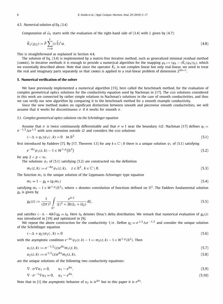
Fig. 1. Smooth example conductivity, its inverse, and the corresponding Schrödinger potentials. In each plot z1 and z2 both range in the interval [−1,1].

5.2. Connection between the cgo solutions ψ1,ψ2 and fμ

From (1.6) we see that −μ relates to 1/σ the same way that μ relates to σ . Set

h+ = 1

2( fμ + f−μ), h− = 1

2( fμ − f−μ);

note that the above definition of h− differs from [1] by an i. Now h+ − ih− and i(h+ + ih−) are solutions of (5.9) and (5.10),respectively, and by uniqueness u1 = h+ − ih− and u2 = i(h+ + ih−). So we can write

fμ = (u1 + u1)/2 + (u2 − u2)/2,

and substituting (1.8), (5.7) and (5.8) gives the desired connection:

ω(z,k) = −1 + e−ikz[Re(σ−1/2eikzm1(z,k)

) + i Im(σ 1/2eikzm2(z,k)

)]. (5.11)

5.3. Computational results

We define a smooth example conductivity σ resembling the transversal cross-section of human chest. The region ofhigher conductivity than background simulates a heart filled with blood, while the two regions with lower conductivitythan background model lungs filled with air. See Fig. 1 for plots of conductivities σ and 1/σ and their respective potentialsq1 and q2.

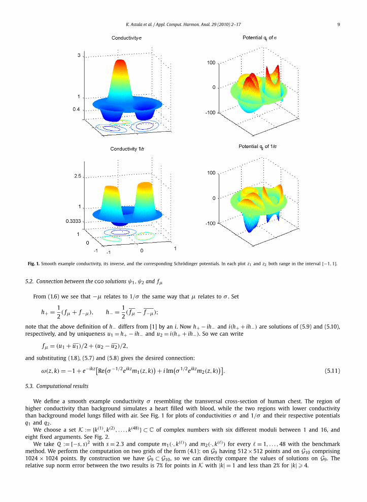
We choose a set K := {k(1),k(2), . . . ,k(48)} ⊂ C of complex numbers with six different moduli between 1 and 16, andeight fixed arguments. See Fig. 2.

We take Q := [−s, s)2 with s = 2.3 and compute m1(·,k(�)) and m2(·,k(�)) for every � = 1, . . . ,48 with the benchmarkmethod. We perform the computation on two grids of the form (4.1): on G9 having 512 × 512 points and on G10 comprising1024 × 1024 points. By construction we have G9 ⊂ G10, so we can directly compare the values of solutions on G9. Therelative sup norm error between the two results is 7% for points in K with |k| = 1 and less than 2% for |k| � 4.

10 K. Astala et al. / Appl. Comput. Harmon. Anal. 29 (2010) 2–17

Fig. 2. Black dots denote the complex points k(1),k(2), . . . ,k(48) used for testing the accuracy of the computation of cgo solutions. The radii of the points inthe collection are indicated on the real axis. The origin of the k plane is in the center of the picture.

Next we evaluate ω̃L(·,k(�)) for � = 1, . . . ,48 on grids G8 and G9. For this, we introduce a radially piecewise linear cutofffunction

η(z) =⎧⎨⎩

1 for |z| < 2.07,

linear for 2.07 � |z| < 2.3,

0 for |z| � 2.3.

According to the theory, of course, the function η should be infinitely smooth as in (2.8). However, we believe that inpractical computation the piecewise linear cutoff function performs well enough.

The computation of the function ω̃L(·,k) defined in (3.4) for a given k ∈ C and z-grid G proceeds as follows.

Step 1. For every z ∈ G , evaluate the functions α(z) and ν(z) defined in (2.2) and (2.3), respectively.Step 2. For every z ∈ G , evaluate the function χΩ(z). Then compute K̃ L(χΩ) using formula (3.1) involving α(z) and ν(z)

available from the previous step. The Cauchy and Beurling transforms appearing in (3.1) are implemented as ex-plained in Sections 4.2 and 4.3, respectively. We use τ = 10−5 as the tolerance in the criterion (4.7) for L.

Step 3. Numerical solution of Eq. (3.4) for ω̃L(·,k) is based on the iterative gmres solver, as explained in Section 4.5. Theright-hand side of (3.4) is now available from the previous step.

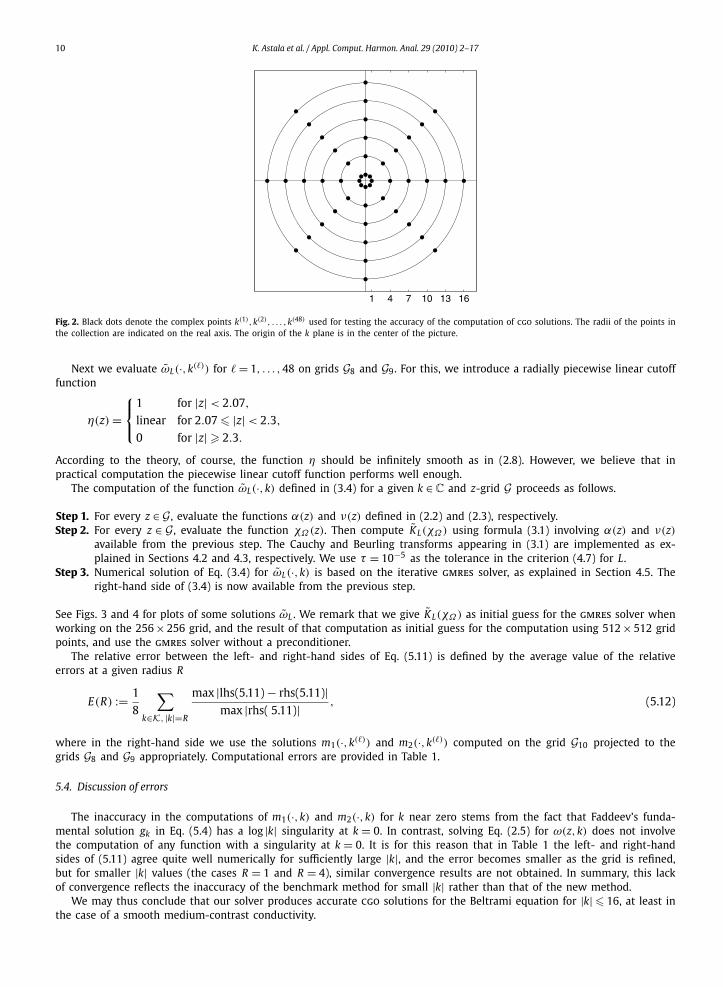
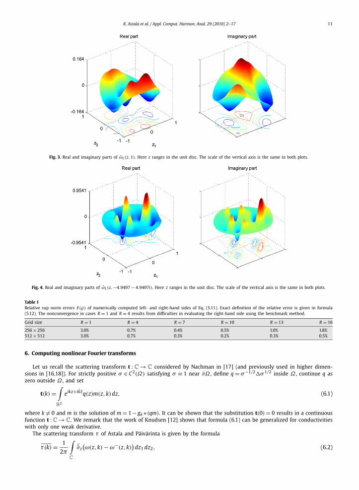
See Figs. 3 and 4 for plots of some solutions ω̃L . We remark that we give K̃ L(χΩ) as initial guess for the gmres solver whenworking on the 256 × 256 grid, and the result of that computation as initial guess for the computation using 512 × 512 gridpoints, and use the gmres solver without a preconditioner.

The relative error between the left- and right-hand sides of Eq. (5.11) is defined by the average value of the relativeerrors at a given radius R

E(R) := 1

8

∑k∈K, |k|=R

max |lhs(5.11) − rhs(5.11)|max |rhs( 5.11)| , (5.12)

where in the right-hand side we use the solutions m1(·,k(�)) and m2(·,k(�)) computed on the grid G10 projected to thegrids G8 and G9 appropriately. Computational errors are provided in Table 1.

5.4. Discussion of errors

The inaccuracy in the computations of m1(·,k) and m2(·,k) for k near zero stems from the fact that Faddeev’s funda-mental solution gk in Eq. (5.4) has a log |k| singularity at k = 0. In contrast, solving Eq. (2.5) for ω(z,k) does not involvethe computation of any function with a singularity at k = 0. It is for this reason that in Table 1 the left- and right-handsides of (5.11) agree quite well numerically for sufficiently large |k|, and the error becomes smaller as the grid is refined,but for smaller |k| values (the cases R = 1 and R = 4), similar convergence results are not obtained. In summary, this lackof convergence reflects the inaccuracy of the benchmark method for small |k| rather than that of the new method.

We may thus conclude that our solver produces accurate cgo solutions for the Beltrami equation for |k| � 16, at least inthe case of a smooth medium-contrast conductivity.

K. Astala et al. / Appl. Comput. Harmon. Anal. 29 (2010) 2–17 11

Fig. 3. Real and imaginary parts of ω̃L(z,1). Here z ranges in the unit disc. The scale of the vertical axis is the same in both plots.

Fig. 4. Real and imaginary parts of ω̃L(z,−4.9497 − 4.9497i). Here z ranges in the unit disc. The scale of the vertical axis is the same in both plots.

Table 1Relative sup norm errors E(�) of numerically computed left- and right-hand sides of Eq. (5.11). Exact definition of the relative error is given in formula(5.12). The nonconvergence in cases R = 1 and R = 4 results from difficulties in evaluating the right-hand side using the benchmark method.

Grid size R = 1 R = 4 R = 7 R = 10 R = 13 R = 16

256 × 256 3.0% 0.7% 0.4% 0.5% 1.0% 1.8%512 × 512 3.0% 0.7% 0.3% 0.2% 0.3% 0.5%

6. Computing nonlinear Fourier transforms

Let us recall the scattering transform t : C → C considered by Nachman in [17] (and previously used in higher dimen-sions in [16,18]). For strictly positive σ ∈ C2(Ω) satisfying σ ≡ 1 near ∂Ω , define q = σ−1/2�σ 1/2 inside Ω , continue q aszero outside Ω , and set

t(k) =∫

R2

eikz+ikzq(z)m(z,k)dz, (6.1)

where k �= 0 and m is the solution of m = 1− gk ∗(qm). It can be shown that the substitution t(0) = 0 results in a continuousfunction t : C → C. We remark that the work of Knudsen [12] shows that formula (6.1) can be generalized for conductivitieswith only one weak derivative.

The scattering transform τ of Astala and Päivärinta is given by the formula

τ (k) = 1

2π

∫∂ z

(ω(z,k) − ω−(z,k)

)dz1 dz2, (6.2)

C

12 K. Astala et al. / Appl. Comput. Harmon. Anal. 29 (2010) 2–17

where ω−(z,k) corresponds to −μ in the same way that ω corresponds to μ. For sufficiently smooth σ , the followingformula gives a connection between the scattering transforms (6.1) and (6.2):

t(k) = −4π ikτ (k). (6.3)

However, the right-hand side of (6.3) is defined for L∞ conductivities as well.The term nonlinear Fourier transform stems from the fact that linearizing t with respect to q by substituting 1 in place

of m in the right-hand side of (6.1) gives the Fourier transform of q. Of course, this interpretation is not strictly valid fort defined via (6.3) for nonsmooth σ since q is no more defined as a function. However, we continue to use the term in ageneralized sense.

Now let Λσ and Λ1 be the Dirichlet to Neumann maps corresponding to σ and the constant conductivity 1, respectively.In medical electric impedance tomography one is dealing with a discontinuous (piecewise smooth) conductivity σ , and (6.1)is not defined. However, the formula

texp(k) =∫

∂Ω

eikz(Λσ − Λ1)eikz dS(z) (6.4)

is a kind of Born approximation, introduced in [19] and makes sense for L∞ conductivities as well. Further, as shown in [13,15], texp(k) can be used to approximate t(k) at least for k near zero and σ smooth. Using texp in practical reconstructionsfrom measured data is known to produce useful images [10,11].

Thus, it is interesting to compare texp(k) to the right-hand side of (6.3) in case of discontinuous conductivities. Such acomparison has so far been possible only for differentiable conductivities.

6.1. Approximate computation of t

We numerically evaluate the functions ω̃L(z,k) and ω̃−L (z,k) and the approximation τL to (6.2) defined by

τL(k) := 1

2π

∫Ω

∂ z(ω̃L(z,k) − ω̃−

L (z,k))

dz1 dz2. (6.5)

The results of Sections 2 and 3 can be used to show that the error in ω̃L(z,k) and ω̃−L (z,k) becomes small when L is large.

Theorem 4. Let τ be defined by (6.2) and τL by (6.5). Then for any k ∈ C

limL→∞τL(k) = τ (k).

Proof. Recall that

∂ω = (I − e−kμS)−1(αω + α),

∂ω− = −(I + e−kμS)−1(αω + α).

Expanding the Neumann series and using the fact that μ is supported in Ω shows that

∂ω(z,k) = 0 and ∂ω−(z,k) = 0 when |z| > 1.

It follows from (6.2) and Theorem 2 that

τ (k) = 1

2π

∫Ω

∂ z(ω̃(z,k) − ω̃−(z,k)

)dz1 dz2. (6.6)

Note that the domain of integration in (6.6) is Ω , while in (6.2) it is R2.

Let ε > 0 be as in (2.8) and define an annulus Aε as follows:

Aε := {z ∈ C

∣∣ 1 < |z| < 1 + ε/2}.

The constructions in the proof of Theorem 2 implies that

∂ zω̃(z,k) = 0 = ∂ zω̃−(z,k) for z ∈ Aε, (6.7)

so we can write using Stokes’ formula

τ (k) = 1

2π

∫|z|<1+ε/4

∂ z(ω̃(z,k) − ω̃−(z,k)

)dz1 dz2

= 1

2π

∫ (ω̃(z,k) − ω̃−(z,k)

)dS(z). (6.8)

|z|=1+ε/4

K. Astala et al. / Appl. Comput. Harmon. Anal. 29 (2010) 2–17 13

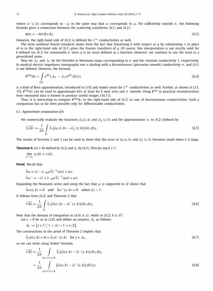
Fig. 5. Left column: profiles of two rotationally symmetric example conductivities with a jump discontinuity. Right column: profiles of texp (thick solid line)and t (thin dotted line) evaluated using Eq. (6.3). Note that texp and t are not expected to coincide.

The construction in the proof of Theorem 3 implies that

∂ zω̃L(z,k) = 0 = ∂ zω̃−L (z,k) for z ∈ Aε, (6.9)

so applying Stokes’ formula to (6.5) leads to

τL(k) = 1

2π

∫|z|=1+ε/4

(ω̃L(z,k) − ω̃−

L (z,k))

dS(z). (6.10)

Formulas (6.7) and (6.9) show that the functions ω̃(·,k), ω̃−(·,k), ω̃L(·,k) and ω̃−L (·,k) are analytic in Aε , and Theorem 3

shows that

limL→∞

∥∥ω̃(·,k) − ω̃L(·,k)∥∥

L2(Aε )= 0,

limL→∞

∥∥ω̃−(·,k) − ω̃−L (·,k)

∥∥L2(Aε )

= 0.

Now L2 convergence and analyticity combined implies pointwise convergence, so the integral in (6.10) converges to theintegral in (6.8) as L → ∞. �6.2. Numerical results for rotationally symmetric cases

Let us define two simple conductivities with rotational symmetry and a jump discontinuity:

σ1(z) ={

1.1 for |z| < 1/2,

1 otherwise,σ2(z) =

{2 for |z| < 1/2,

1 otherwise.

See the left column of Fig. 5 for plots of profiles of σ1 and σ2.It is well known that the Dirichlet-to-Neumann maps Λσ1 and Λσ2 can be expanded analytically in the trigonometric

basis on the unit circle, see e.g. [19, Lemma 4.1]. Utilizing this we evaluate texp1 (k) and texp

2 (k) very accurately with formula(6.4), see the solid line plots in the right column of Fig. 5.

We evaluate ω̃L(z,k) and ω̃−L (z,k) corresponding to both conductivities using the algorithm described in Section 4.

Here k is real-valued and ranges in the interval [0.1,19.6]. It is enough to compute using real k only since the symmetryσ(z) = σ(|z|) implies texp(k) = texp(|k|) and t(k) = t(|k|).

14 K. Astala et al. / Appl. Comput. Harmon. Anal. 29 (2010) 2–17

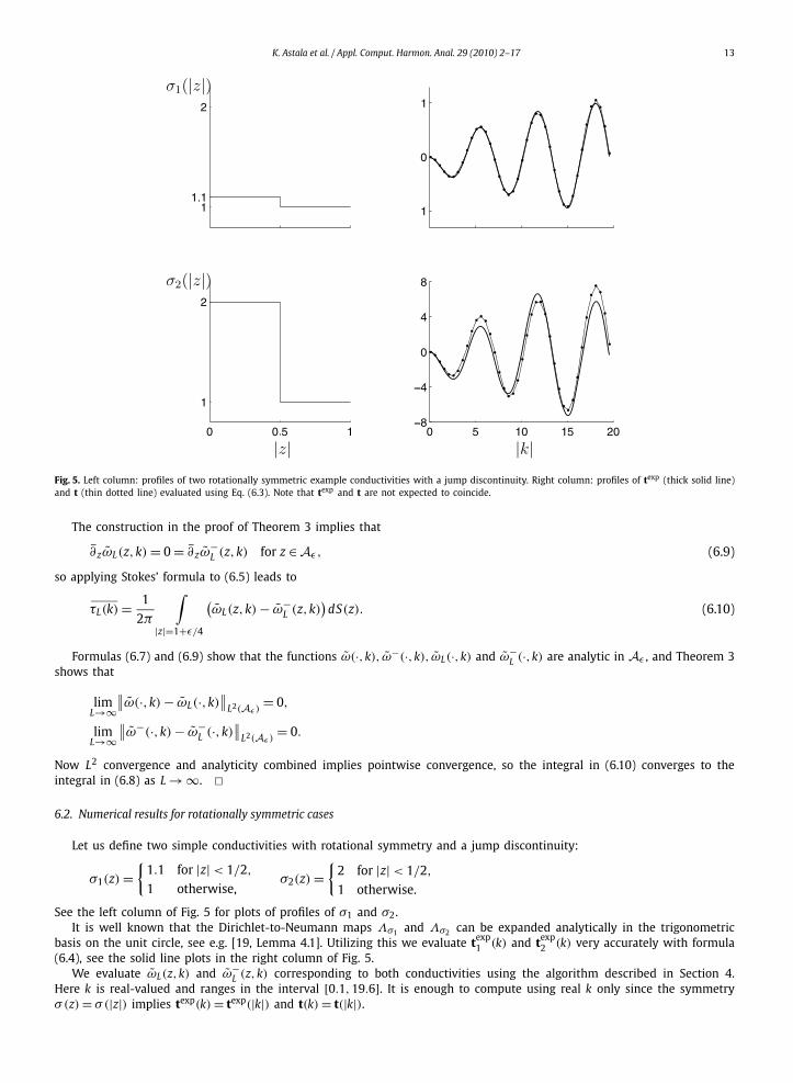
Fig. 6. Left: profile of the rotationally symmetric example conductivity σ3. Right: approximate profiles of t computed using the benchmark method (thicksolid line) and the new method (thin dotted line); note that these two functions are expected to coincide, but there is significant difference between themnear k = 0. This is due to the inaccuracy of the benchmark method; the new algorithm performs clearly better for small k since t is a continuous functionand t(0) = 0. For large |k| the computations agree remarkably well.

Since the conductivities are nonsmooth, we cannot use the benchmark method for checking the accuracy of the compu-tation by comparison as in Section 5.3. Instead we compute ω̃L(z,k) and ω̃−

L (z,k) on the two grids G8 and G9, and comparethe results on the points belonging to G8. The relative sup norm error between the two computations is less than 5% fork < 6.6, less than 10% for k < 12.6, and at most 21% in the whole k interval. Of course, we expect the result computed on

G9 to be more accurate, as is the case in the situation summarized in Table 1. Thus we have good reason to believe that thecomputation is reasonably accurate in the whole k interval.

We can now evaluate the scattering transforms t1 and t2 using (6.5) and (6.3). The functions t1 and t2 are plotted withthin dotted lines in the right column of Fig. 5.

As mentioned above, there is inaccuracy in the computation of ω̃L(z,k) and ω̃−L (z,k). Also, numerical differentiation in

the implementation of the right-hand side of (6.5) may amplify the errors. Thus it is reasonable to doubt the accuracy ofthe plot of t(k) in Fig. 5, especially for large |k|. Let us make one more numerical test to estimate the size of error.

We define one more rotationally symmetric conductivity called σ3 as follows: define ζ(t) := 1 − 10t3 + 15t4 − 6t5 andset

σ3(z) =⎧⎨⎩

2 for |z| < 3/10,

1 for |z| > 7/10,

1 + ζ( 10(|z|−3/10)

4

)otherwise.

See the left plot of Fig. 6 for the profile of σ3. Now σ3 ∈ C4(Ω) so that we can evaluate t using the benchmark method andformula (6.1). The right plot of Fig. 6 shows the results of these two methods of computation. For large |k| they agree verynicely, and for small |k| there is significant error. The inaccuracy near the origin comes from the benchmark algorithm sincet is known to be a continuous function and t(0) = 0, so the new method is seen to be accurate for small |k| as well. Thetest thus suggests that the computations in Fig. 5 are accurate.

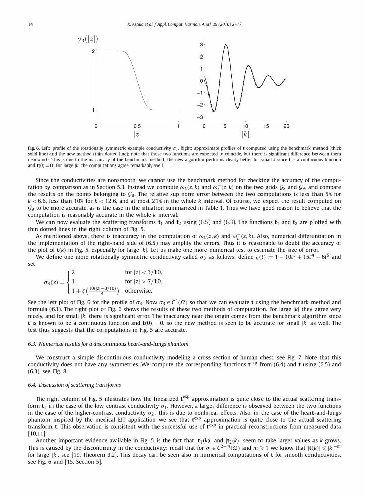
6.3. Numerical results for a discontinuous heart-and-lungs phantom

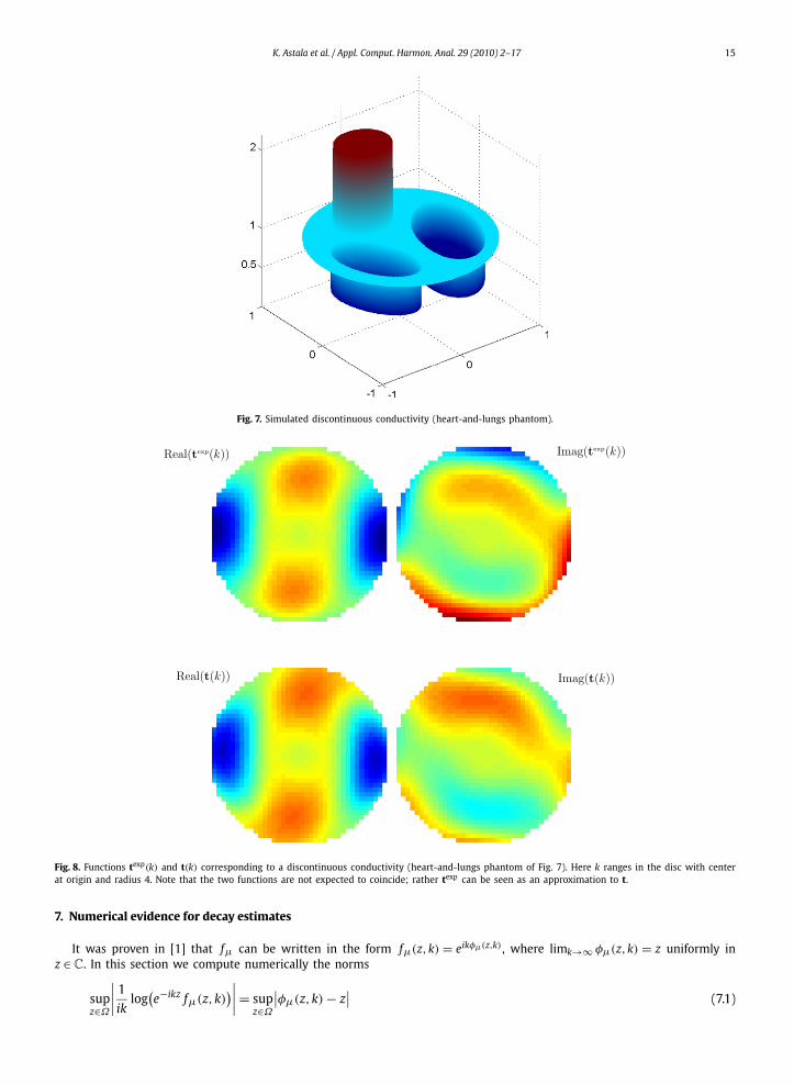
We construct a simple discontinuous conductivity modeling a cross-section of human chest, see Fig. 7. Note that thisconductivity does not have any symmetries. We compute the corresponding functions texp from (6.4) and t using (6.5) and(6.3), see Fig. 8.

6.4. Discussion of scattering transforms

The right column of Fig. 5 illustrates how the linearized texp1 approximation is quite close to the actual scattering trans-

form t1 in the case of the low contrast conductivity σ1. However, a larger difference is observed between the two functionsin the case of the higher-contrast conductivity σ2; this is due to nonlinear effects. Also, in the case of the heart-and-lungsphantom inspired by the medical EIT application we see that texp approximation is quite close to the actual scatteringtransform t. This observation is consistent with the successful use of texp in practical reconstructions from measured data[10,11].

Another important evidence available in Fig. 5 is the fact that |t1(k)| and |t2(k)| seem to take larger values as k grows.This is caused by the discontinuity in the conductivity: recall that for σ ∈ C2+m(Ω) and m � 1 we know that |t(k)| � |k|−m

for large |k|, see [19, Theorem 3.2]. This decay can be seen also in numerical computations of t for smooth conductivities,see Fig. 6 and [15, Section 5].

K. Astala et al. / Appl. Comput. Harmon. Anal. 29 (2010) 2–17 15

Fig. 7. Simulated discontinuous conductivity (heart-and-lungs phantom).

Fig. 8. Functions texp(k) and t(k) corresponding to a discontinuous conductivity (heart-and-lungs phantom of Fig. 7). Here k ranges in the disc with centerat origin and radius 4. Note that the two functions are not expected to coincide; rather texp can be seen as an approximation to t.

7. Numerical evidence for decay estimates

It was proven in [1] that fμ can be written in the form fμ(z,k) = eikφμ(z,k) , where limk→∞ φμ(z,k) = z uniformly inz ∈ C. In this section we compute numerically the norms

sup

∣∣∣∣ 1

iklog

(e−ikz fμ(z,k)

)∣∣∣∣ = sup∣∣φμ(z,k) − z

∣∣ (7.1)

z∈Ω z∈Ω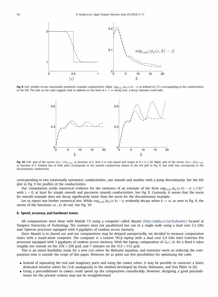

16 K. Astala et al. / Appl. Comput. Harmon. Anal. 29 (2010) 2–17

Fig. 9. Left: profiles of two rotationally symmetric example conductivities. Right: supz∈Ω |φμ(z,k)− z| as defined in (7.1) corresponding to the conductivitiesto the left. The plot on the right suggests that in addition to the limit at k → ∞ being zero, a decay estimate could hold.

Fig. 10. Left: plot of the norms ‖ω̃L(·,k)‖L2(Ω) as function of k; here k is real-valued and ranges in 0 � k � 20. Right: plot of the norms ‖ω̃L(·,k)‖L∞(Ω)

as function of k. Dashed line in both plots corresponds to the smooth conductivity shown in the left plot in Fig. 9, and solid line corresponds to thediscontinuous conductivity.

corresponding to two rotationally symmetric conductivities, one smooth and another with a jump discontinuity. See the leftplot in Fig. 9 for profiles of the conductivities.

Our computation yields numerical evidence for the existence of an estimate of the form supz∈Ω |φμ(z,k) − z| � C |k|λwith λ < 0, at least for simple smooth and piecewise smooth conductivities. See Fig. 9. Curiously, it seems that the normfor smooth example does not decay significantly faster than the norm for the discontinuous example.

Let us report one further numerical test. While supz∈Ω |φμ(z,k) − z| evidently decays when k → ∞ as seen in Fig. 9, thenorms of the functions ω(·,k) do not. See Fig. 10.

8. Speed, accuracy, and hardware issues

All computations were done with Matlab 7.5 using a computer called Akaatti (http://alpha.cc.tut.fi/akaatti/) located atTampere University of Technology. The routines were not parallelized but run in a single node using a dual core 2.2 GHzamd Opteron processor equipped with 4 gigabytes of random access memory.

Since Akaatti is in shared use and our computations may be delayed unexpectedly, we decided to measure computationtimes with a stand-alone computer. The computer is a Lenovo T61p laptop with a dual core 2.4 GHz Intel Centrino Proprocessor equipped with 3 gigabytes of random access memory. With the laptop, computation of ω̃L(·,k) for a fixed k takesroughly one minute on the 256 × 256 grid, and 7 minutes on the 512 × 512 grid.

This is an initial feasibility study for a new cgo solver for Beltrami equation, and extensive work on reducing the com-putation time is outside the scope of this paper. However, let us point out few possibilities for optimizing the code:

• Instead of separating the real and imaginary parts and using the gmres solver, it may be possible to construct a fasterdedicated iterative solver for (3.4) analogously to the method developed by Eirola, Huhtanen, and Von Pfaler in [6].

• Using a preconditioner in gmres could speed up the computation considerably. However, designing a good precondi-tioner for the present context may not be straightforward.

K. Astala et al. / Appl. Comput. Harmon. Anal. 29 (2010) 2–17 17

• Our algorithm is naturally parallelizable since computation of ω̃L(z,k) can be done independently for each k value.• Our approach could allow a two-grid extension similarly to the Lippmann–Schwinger case discussed in [22].

Full accuracy analysis for the new method would be valuable. This may require some refinements in the algorithm, suchas more careful grid approximation for piecewise smooth functions as explained in [22].

Acknowledgments

This material is based upon work supported by the National Science Foundation under Grant No. 0513509 (J. Mueller)and by the Finnish Centre of Excellence in Inverse Problems Research (Academy of Finland CoE-project 213476, L. Päivärintaand S. Siltanen) and by the Finnish Center of Excellence in Analysis and Dynamics Research (Academy of Finland projects1118634 and 118422, K. Astala). During part of the preparation of this work, S.S. worked as professor at the Department ofMathematics of Tampere University of Technology.

References

[1] K. Astala, L. Päivärinta, Calderón’s inverse conductivity problem in the plane, Ann. of Math. 163 (2006) 265–299.[2] J. Bikowski, J.L. Mueller, 2D EIT reconstructions using Calderón’s method, Inverse Probl. Imaging 2 (2007) 43–61.[3] A.P. Calderón, On an inverse boundary value problem, in: Seminar on Numerical Analysis and Its Applications to Continuum Physics, Soc. Brasileira de

Matemàtica, 1980, pp. 65–73.[4] M. Cheney, D. Isaacson, J.C. Newell, Electrical impedance tomography, SIAM Rev. 41 (1999) 85–101.[5] P. Daripa, A fast algorithm to solve the Beltrami equation with applications to quasiconformal mappings, J. Comput. Phys. 106 (1993) 355–365.[6] T. Eirola, M. Huhtanen, J. Von Pfaler, Solution methods for R-linear problems in C

n , SIAM J. Matrix Anal. Appl. 25 (2003) 804–828.[7] L.D. Faddeev, Increasing solutions of the Schrödinger equation, Sov. Phys. Dokl. 10 (1966) 1033–1035.[8] D. Gaydashev, D. Khmelev, On numerical algorithms for the solution of a Beltrami equation, arXiv:math.NA/0510516, 2005.[9] M. Ikehata, S. Siltanen, Numerical solution of the Cauchy problem for the stationary Schrödinger equation using Faddeev’s Green function, SIAM J.

Appl. Math. 64 (2004) 1907–1932.[10] D. Isaacson, J.L. Mueller, J. Newell, S. Siltanen, Reconstructions of chest phantoms by the d-bar method for electrical impedance tomography, IEEE

Trans. Med. Imaging 23 (2004) 821–828.[11] D. Isaacson, J.L. Mueller, J. Newell, S. Siltanen, Imaging cardiac activity by the d-bar method for electrical impedance tomography, Physiol. Meas. 27

(2006) S43–S50.[12] K. Knudsen, On the inverse conductivity problem, Ph.D. thesis, Department of Mathematical Sciences, Aalborg University, Denmark, 2002.[13] K. Knudsen, M. Lassas, J.L. Mueller, S. Siltanen, D-bar method for electrical impedance tomography with discontinuous conductivities, SIAM J. Appl.

Math. 67 (2007) 893–913.[14] K. Knudsen, J.L. Mueller, S. Siltanen, Numerical solution method for the dbar-equation in the plane, J. Comput. Phys. 198 (2004) 500–517.[15] J.L. Mueller, S. Siltanen, Direct reconstructions of conductivities from boundary measurements, SIAM J. Sci. Comput. 24 (2003) 1232–1266.[16] A.I. Nachman, Reconstructions from boundary measurements, Ann. of Math. 128 (1988) 531–576.[17] A.I. Nachman, Global uniqueness for a two dimensional inverse boundary value problem, Ann. of Math. 143 (1996) 71–96.[18] R.G. Novikov, G.M. Khenkin, The ∂-equation in the multidimensional inverse scattering problem, Uspekhi Mat. Nauk 42 (1987) 93–152.[19] S. Siltanen, J. Mueller, D. Isaacson, An implementation of the reconstruction algorithm of A. Nachman for the 2-D inverse conductivity problem, Inverse

Problems 16 (2000) 681–699.[20] E. Stein, Singular Integrals and Differentiability Properties of Functions, Princeton Mathematical Series, vol. 30, Princeton University Press, Princeton,

NJ, 1970.[21] J. Sylvester, G. Uhlmann, A global uniqueness theorem for an inverse boundary value problem, Ann. of Math. 125 (1987) 153–169.[22] G. Vainikko, Fast solvers of the Lippmann–Schwinger equation, in: Direct and Inverse Problems of Mathematical Physics, Newark, DE, in: Int. Soc. Anal.

Appl. Comput., vol. 5, Kluwer Acad. Publ., Dordrecht, 2000, p. 423.