DIRICHLET-TO-NEUMANN FINITE ELEMENT …koyama/thesis.pdfFINITE ELEMENT METHODS FOR WAVE PROBLEMS BY Daisuke Koyama A DISSERTATION SUBMITTED IN PARTIAL FULFILLMENT OF THE REQUIREMENTS

DIRICHLET-TO-NEUMANN

FINITE ELEMENT METHODS FOR

WAVE PROBLEMS

BY

Daisuke Koyama

A DISSERTATION

SUBMITTED IN PARTIAL FULFILLMENT OF THEREQUIREMENTS FOR THE DEGREE OF

DOCTOR OF SCIENCE

AT

THE UNIVERSITY OF ELECTRO-COMMUNICATIONSSEPTEMBER 2006

DIRICHLET-TO-NEUMANN

FINITE ELEMENT METHODS FOR

WAVE PROBLEMS

APPROVED BY SUPERVISORY COMMITTEE:

CHAIRPERSON: Professor Takashi Kako

MEMBER: Professor Kohei NoshitaMEMBER: Professor Toshiki Naito

MEMBER: Professor Fumio KikuchiMEMBER: Professor Nobito Yamamoto

MEMBER: Professor Hidenori Ogata

Copyright 2006 by Daisuke Koyama

波動問題に対するDirichlet-to-Neumann有限要素法

小　山　大　介　

概要

凹角を持つ水域における水の波の線型固有値問題と外部 Helmholtz問題に対する Dirichlet-to-Neumann (DtN)有限要素法の事前誤差評価を導出する．水の波の線型固有値問題の場合には，導出した誤差評価の正当性を保証する数値例を与える．外部Helmholtz問題の場合には，より良い評価を得るために，Hankel関数の新たな性質を証明する．外部 Helmholtz問題を解くための可制御法に適した，波動方程式に対す

るあるDtN 境界条件を提案する．この境界条件下での波動方程式の一意可解性を証明する．Helmholtz問題と可制御法において生ずるある制御問題の同値性について考察する．三次元外部 Helmholtz問題を解くための仮想領域法の一つの定式化を与

える．その離散問題で生ずる制約行列の要素計算アルゴリズムを与える．さらに，このアルゴリズムは数値誤差の影響で破綻しないことを示す．

i

Dirichlet-to-NeumannFinite Element Methods for

Wave Problems

Daisuke Koyama

Abstract

The Dirichlet-to-Neumann (DtN) finite element method is applied to theeigenvalue problem of the linear water wave in a water region with a reentrantcorner and to the exterior Helmholtz problem.

Error estimates of the DtN finite element methods for these problemsare established. The error estimates include the effect of truncation of theinfinite series representing the DtN boundary condition as well as that of thefinite element discretization.

In the case of the eigenvalue problem of the linear water wave, the errorestimates assure that the DtN finite element method improves the deteriora-tion of convergence rate caused by the corner singularity. Numerical examplesare presented which illustrate this improvement.

In the case of the Helmholtz problem, a new property of the Hankelfunctions is proved to get a sharp estimation of the error caused by thetruncation.

A certain DtN boundary condition for the time-dependent wave equationis proposed which is suitable to the controllability method for solving theexterior Helmholtz problem. The well-posedness of the wave equation im-posing the DtN boundary condition is established by using the semi-grouptheory. Equivalence between the Helmholtz problem and an exact control-lability problem arising in the controllability method is investigated. A suf-ficient condition for the equivalence is presented in discrete level. A typicalexample is shown where the condition is satisfied. Some numerical examplesare also presented which verify the validity of the controllability method withthe DtN boundary condition.

A fictitious domain formulation using the Lagrange multipliers is pre-sented for the 3D Helmholtz problem imposing the DtN boundary condition.

ii

An algorithm for computing the constraint matrices in the linear systemarising in finite element discretizations is presented. In the algorithm, a tri-angulation algorithm for the intersection of a tetrahedron and a triangle playsan essential role. The triangulation algorithm is shown to be numerically ro-bust, and further is simplified. The effectiveness of the simplified algorithmis shown through some numerical experiments.

iii

Acknowledgements

I would like to thank my adviser, Professor Takashi Kako, for many pieces ofvaluable and insightful advice, for his constant encouragement, for creating awarm atmosphere, and for his various classes throughout my undergraduateand graduate educations. I owe him more gratitude than I can express. I waslucky to meet him when I was a freshman at the Department of Mathematicsof Saitama University in April 1987, and to study and work close to him eversince. For the period of nineteen and a half years, I have learned a lot ofthings in various phases from him.

I wish to express my gratitude to Emeritus Professor Teruo Ushijima forhis support and valuable suggestions. He introduced the DtN finite elementmethod to me, and suggested me that I should establish error estimatesof the DtN finite element method for the eigenvalue problem of the linearwater wave equation in a water region with a reentrant corner, and shouldinvestigate the equivalence between the Helmholtz problem and the exactcontrollability problem in discrete level.

I would like to express my thanks to Professor Fumio Kikuchi for servingon a member of the examining committee of my dissertation and for hishospitality during a visit to the Graduate School of Mathematical Sciencesof University of Tokyo, where I devised the algorithm for computing theconstraint matrix.

I would also like to express my thanks to Professors Kohei Noshita,Toshiki Naito, Nobito Yamamoto, and Hidenori Ogata for serving on mem-bers of the examining committee of my dissertation.

I would like to extend my thanks to Mr. Makoto Fukuhara for providingadministrative support of computer facilities, and to Dr. Ken-Ichi Nakamuraand Dr. Toshiyuki Imamura, who provided computer facilities which theyhas administered.

Special thanks are due to Mr. Kazuhiro Ishii, Mr. Isao Takanami, and

iv

Mr. Katsuhiko Tanimoto, who instructed me in the use of the computer.This work could not have been completed without the unconditional sup-

port from my mother and my brother. I thank my mother for bring me upall by herself.

v

Contents

1 Introduction 11.1 The linear water wave problem . . . . . . . . . . . . . . . . . 11.2 The Helmholtz problem . . . . . . . . . . . . . . . . . . . . . 31.3 The Dirichlet-to-Neumann (DtN) finite element method . . . . 41.4 Topics of the thesis . . . . . . . . . . . . . . . . . . . . . . . . 11

1.4.1 Error analysis of the DtN finite element method . . . . 111.4.2 The controllability method . . . . . . . . . . . . . . . . 111.4.3 The fictitious domain method . . . . . . . . . . . . . . 13

1.5 Organization of the thesis . . . . . . . . . . . . . . . . . . . . 151.6 Notations . . . . . . . . . . . . . . . . . . . . . . . . . . . . . 16

I The Eigenvalue Problem of the Linear Water Wavein a Water Region with a Reentrant Corner 18

2 The DtN Finite Element Method 192.1 The eigenvalue problem of the linear water wave . . . . . . . . 192.2 The DtN operator and the reduced problem . . . . . . . . . . 222.3 The discrete approximation problem and main theorems . . . 292.4 Preliminary consideration for error estimate . . . . . . . . . . 32

2.4.1 Estimate for the truncation error . . . . . . . . . . . . 332.4.2 Estimate for the discretization error . . . . . . . . . . . 36

2.5 Proof of the main theorems . . . . . . . . . . . . . . . . . . . 372.6 Numerical results . . . . . . . . . . . . . . . . . . . . . . . . . 43

2.6.1 Rates of convergence for the standard finite elementmethod . . . . . . . . . . . . . . . . . . . . . . . . . . 44

2.6.2 Rates of convergence for the DtN finite element method 462.7 Conclusions . . . . . . . . . . . . . . . . . . . . . . . . . . . . 47

vi

II The Exterior Helmholtz Problem 53

3 The DtN Finite Element Method 543.1 The exterior Helmholtz problem . . . . . . . . . . . . . . . . . 543.2 The DtN formulation . . . . . . . . . . . . . . . . . . . . . . . 553.3 The DtN finite element method and its error estimates . . . . 583.4 Conclusions . . . . . . . . . . . . . . . . . . . . . . . . . . . . 66

4 The Controllability Method 674.1 An exact controllability problem . . . . . . . . . . . . . . . . . 674.2 Discussion of the uniqueness for problem (4.2) . . . . . . . . . 684.3 Uniqueness of the solution to semi-discrete problems of prob-

lem (4.2) . . . . . . . . . . . . . . . . . . . . . . . . . . . . . . 694.4 An example satisfying condition 1 . . . . . . . . . . . . . . . . 754.5 Procedure of the controllability method . . . . . . . . . . . . . 80

4.5.1 Computation of Ahvh . . . . . . . . . . . . . . . . . . 834.6 Numerical examples . . . . . . . . . . . . . . . . . . . . . . . . 85

4.6.1 Scattering by a disk . . . . . . . . . . . . . . . . . . . . 864.6.2 Scattering by a Π-shaped open resonator . . . . . . . . 86

4.7 Conclusions . . . . . . . . . . . . . . . . . . . . . . . . . . . . 88

5 The Fictitious Domain Method 905.1 A fictitious domain formulation . . . . . . . . . . . . . . . . . 905.2 Algorithm for computing the constraint matrix Bγ . . . . . . . 97

5.2.1 Triangulation algorithm for the intersection of a tetra-hedron and a triangle . . . . . . . . . . . . . . . . . . . 98

5.2.2 Algorithm for computing the entries of matrix Bγ . . . 1025.2.3 The effect of numerical error . . . . . . . . . . . . . . . 103

5.3 Simplification of the algorithm . . . . . . . . . . . . . . . . . . 1055.4 Numerical experiments . . . . . . . . . . . . . . . . . . . . . . 1075.5 Conclusions . . . . . . . . . . . . . . . . . . . . . . . . . . . . 110

A Some Properties of the Hankel Functions 116

B Well-posedness of the Wave Equation with a DtN BoundaryCondition 122B.1 Proof of Theorem 4.1 . . . . . . . . . . . . . . . . . . . . . . . 122

B.1.1 Proof of Proposition B.1 . . . . . . . . . . . . . . . . . 123

vii

B.1.2 Proof of Proposition B.2 . . . . . . . . . . . . . . . . . 124B.1.3 Proof of Proposition B.3 . . . . . . . . . . . . . . . . . 125

viii

Chapter 1

Introduction

The boundary value problems of differential equations defined on unboundeddomains or domains with corners often arise in science and engineeringfields. The Dirichlet-to-Neumann (DtN) finite element method is a numericalmethod to solve effectively such problems by excluding the unboundedness orthe corner singularity. We investigate the DtN finite element method appliedto wave problems through mathematical analysis and numerical experiments.As wave problems, we consider the eigenvalue problem of the linear waterwave (the sloshing problem) in a water region with a reentrant corner andthe exterior Helmholtz problem. First, we derive a priori error estimates ofthe DtN finite element methods applied to these problems. Next we considerthe controllability method for solving the exterior Helmholtz problem. Wepropose a DtN boundary condition for the time-dependent wave equationthat is suitable to the controllability method, and discuss the validity of thecontrollability method using such a DtN boundary condition. Finally we pro-pose a fictitious domain formulation for the Helmholtz problem imposing theDtN boundary condition, and present an algorithm for computing the entriesof the constraint matrix arising in such a fictitious domain formulation.

1.1 The linear water wave problem

When wave motion in the water with a free surface is described as a mathe-matical model, the fluid is assumed to be homogeneous, inviscid, and incom-pressible, and its motion is assumed to be irrotational. The last assumptionguarantees the existence of a velocity potential Φ. When the amplitude of

1

the wave motions is small, the velocity potential Φ satisfies the followinglinear initial-boundary value problem:

(1.1)

⎧⎪⎪⎪⎪⎪⎪⎪⎪⎨⎪⎪⎪⎪⎪⎪⎪⎪⎩

−ΔΦ = 0 in Ω,∂2Φ

∂t2+ g

∂Φ

∂n=

∂F

∂ton Γ0,

∂Φ

∂n= 0 on Γ1,

Φ(0) = Φ0 on Γ0,∂Φ

∂t(0) = Φ1 on Γ0,

where Ω denotes the region of the water at rest, Γ0 the surface of the waterat rest, Γ1 the rigid wall in contact with the water at rest, g the accelerationof gravity, n the outward unit normal vector on the boundary of Ω, and Fthe additional external force per unit surface affecting the water surface. Formore details of the derivation of (1.1), see, e.g., [121, 98]. In this thesis, weshall call (1.1) the linear water wave problem.

The eigenvalue problem associated with problem (1.1), i.e., the eigenvalueproblem of the linear water wave is as follows:

(1.2)

⎧⎪⎪⎪⎨⎪⎪⎪⎩−Δu = 0 in Ω,

∂u

∂n= αu on Γ0,

∂u

∂n= 0 on Γ1.

This eigenvalue problem is often called the sloshing problem. Note here thatthe eigenvalues α are related to the sloshing frequencies ω by α = ω2/g. Asis well known, solutions of (1.1) can be given by superposition of eigenvectorsof (1.2) (see [127]).

For a historical review of the sloshing problem (1.2), we refer to [36] andreferences therein. According to [36], we see that the sloshing problem is aclassical problem. In addition, for a historical review of the linear water waveproblem (1.1), see [120, 121, 98].

The sloshing problem is of great concern in aerospace and civil engineeringfields, as exemplified by applications to fuel sloshing in liquid propellantvehicles and seismic loads on dams and liquid storage tanks.

The sloshing problem (1.2) is analytically solved in the cases when thewater region Ω is so simple that separation of variables can be applied to

2

the problem; however, in the cases of general shapes of Ω, approximationmethods are valuable, e.g., in [25] the finite deference method is applied tothe problem in axisymmetric domains, in [106, 42] analytical representationsof approximate solutions are presented in the case when finite differencediscretizations are applied to the problem in rectangular domains, in [37, 38]the problem in axisymmetric domains is solved by the finite element method,and in [94] the DtN finite element method is applied to the problem in two-dimensional domains with a reentrant corner.

1.2 The Helmholtz problem

The wave equation:

(1.3)1

c2

∂2w

∂t2− Δw = F

with the wave speed c, arises in acoustics, elastodynamics, and electromag-netics. Its solutions describe the propagations of acoustic, elastic, and elec-tromagnetic waves (see, e.g., [22, 75]).

In applications, e.g., in the radar technology, most of the time we mayassume that F is time harmonic:

F (x, t) = f(x) exp(−iωt),

where ω is the circular frequency and i =√−1. In this case, we may also

assume that the solution of the wave equation is of the form w(x, t) =u(x) exp(−iωt). Then u satisfies the Helmholtz equation:

−Δu − k2u = f,

where k = ω/c is the wave number and will be assumed to be a positiveconstant in this thesis.

In the stealth technology for radar, the phenomena are described as theexterior Helmholtz problem with the Sommerfeld radiation condition im-posed at infinity:

(1.4)

⎧⎪⎪⎨⎪⎪⎩−Δu − k2u = f in Ω,

u = 0 on γ,

limr−→+∞

rd−12

(∂u

∂r− iku

)= 0,

3

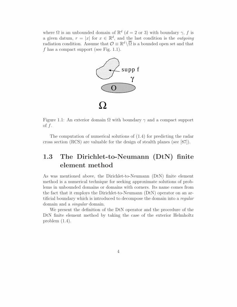
where Ω is an unbounded domain of Rd (d = 2 or 3) with boundary γ, f isa given datum, r = |x| for x ∈ Rd, and the last condition is the outgoingradiation condition. Assume that O ≡ Rd \Ω is a bounded open set and thatf has a compact support (see Fig. 1.1).

γΟ

Ω

supp f

Figure 1.1: An exterior domain Ω with boundary γ and a compact supportof f .

The computation of numerical solutions of (1.4) for predicting the radarcross section (RCS) are valuable for the design of stealth planes (see [87]).

1.3 The Dirichlet-to-Neumann (DtN) finite

element method

As was mentioned above, the Dirichlet-to-Neumann (DtN) finite elementmethod is a numerical technique for seeking approximate solutions of prob-lems in unbounded domains or domains with corners. Its name comes fromthe fact that it employs the Dirichlet-to-Neumann (DtN) operator on an ar-tificial boundary which is introduced to decompose the domain into a regulardomain and a singular domain.

We present the definition of the DtN operator and the procedure of theDtN finite element method by taking the case of the exterior Helmholtzproblem (1.4).

4

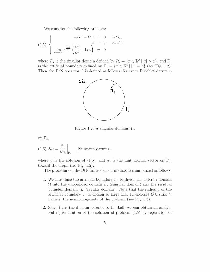
We consider the following problem:

(1.5)

⎧⎪⎪⎨⎪⎪⎩−Δu − k2u = 0 in Ωs,

u = ϕ on Γa,

limr−→∞

rd−12

(∂u

∂r− iku

)= 0,

where Ωs is the singular domain defined by Ωs = {x ∈ Rd | |x| > a}, and Γa

is the artificial boundary defined by Γa = {x ∈ Rd | |x| = a} (see Fig. 1.2).

Then the DtN operator S is defined as follows: for every Dirichlet datum ϕ

Γ

Ω

a

s

ns

Figure 1.2: A singular domain Ωs.

on Γa,

(1.6) Sϕ =∂u

∂ns

∣∣∣∣Γa

(Neumann datum),

where u is the solution of (1.5), and ns is the unit normal vector on Γa,toward the origin (see Fig. 1.2).

The procedure of the DtN finite element method is summarized as follows:

1. We introduce the artificial boundary Γa to divide the exterior domainΩ into the unbounded domain Ωs (singular domain) and the residualbounded domain Ωa (regular domain). Note that the radius a of theartificial boundary Γa is chosen so large that Γa encloses O ∪ supp f ,namely, the nonhomogeneity of the problem (see Fig. 1.3).

2. Since Ωs is the domain exterior to the ball, we can obtain an analyt-ical representation of the solution of problem (1.5) by separation of

5

γΟ

ΓΩ aa

supp f

n

Figure 1.3: A regular domain Ωa.

variables. Using this analytical representation, we obtain an analyticalrepresentation of the DtN operator. We note here that we can alsoobtain an analytical representation of the DtN operator when, as anartificial boundary Γa, we choose an elliptic boundary if d = 2, or aspheroidal one if d = 3 (see [63]).

3. Imposing a boundary condition using the DtN operator, called the DtNboundary condition, on Γa, we reduce the original exterior problem(1.4) equivalently to the following problem:

(1.7)

⎧⎪⎨⎪⎩−Δu − k2u = f in Ωa,

u = 0 on γ,∂u

∂n= −Su on Γa,

where n is the outward unit normal vector on Γa (see Fig. 1.3). Notethat we have n = −ns.

4. We solve (1.7) by the finite element method.

In 1989, Keller–Givoli [86] first called the last equation of (1.7) the DtNboundary condition, and further the above procedures 1–4 the DtN finiteelement method. Before 1989, the DtN boundary condition had been alreadyknown as a boundary condition which is naturally incorporated into the finiteelement procedure; several authors had derived the DtN boundary conditionsfor several problems and had studied the corresponding DtN finite elementmethods.

Examples of such works before 1989 are the following.

6

In 1978, Fix–Marin [35], who are pioneers in the DtN finite elementmethod, derived the DtN boundary condition for the under-water acousticproblem as a generalized radiation condition; the DtN boundary conditionis based on separation of variables and is represented as a Fourier infiniteseries. They presented some numerical examples, where the second orderconvergence of the DtN finite element method in the maximum norm isobserved and a comparison between the DtN boundary condition and theclassical radiation condition is made.

In 1980, MacCamy–Marin [103] represented the DtN boundary conditionfor the exterior Helmholtz problem through an integral equation; such arepresentation is available for general smooth artificial boundaries. Theyfurther established error estimates and presented some numerical exampleswhich confirm such error estimates.

In 1982, Goldstein [56] derived the DtN boundary condition for the Helmholtzproblem on unbounded waveguides; he also represented it through a Fourierinfinite series. Moreover he established error estimates that include the ef-fect of truncation of the infinite series as well as that of discretization of thefinite element method. Further, Seto [117] derived the DtN boundary con-dition associated with the three dimensional water wave radiation problem,and computed practical problems by using it.

In 1983, Feng [31] derived a Fourier series representation of the DtNoperator for the exterior Helmholtz problem, and presented a sequence oflocal artificial boundary conditions which is obtained by approximating theFourier series representation by using an asymptotic expansion of the Hankelfunctions for large arguments. In addition, Feng–Yu [32] derived the DtNboundary conditions for the Laplace, the biharmonic, and the linear elasticequations.

In 1985, Han–Wu [72] established an error estimate for the exterior Laplaceproblem which also estimates the error cause by the truncation of the infiniteseries in the DtN boundary condition as well as the discretization error dueto the finite element method. Yu [138] analyzed, for the same problem, onlythe truncation error.

In 1986, Yu [137] applied the DtN finite element method to the Laplaceproblem with a corner singularity, and proved an error estimate with respectto the mesh size.

In 1987, Masmoudi [105] also proved the same error estimate as in MacCamy–Marin [103] for the exterior Helmholtz problem. He however employed theFourier series representation of the DtN boundary condition, and presented

7

some numerical examples which confirm the error estimate.In 1988, Lenoir–Tounsi [99] established an error estimate of the DtN finite

element method for the two-dimensional water wave radiation problem. Intheir error estimate, the truncation error and the discretization error are bothanalyzed.

After 1989, the DtN finite element method has been applied further tovarious problems.

For problems in unbounded domains, the linear elastic wave problem wereinvestigated by Givoli–Keller [48] for 2D and by Gachter–Grote [40] for 3D;the Stokes problem by Yu [140] for 2D and by Zheng–Han [142] for 3D;and the diffraction problem of a time harmonic wave incident on a periodicsurface of some inhomogeneous material by Bao [6].

For problems with corner singularities, boundary value problems for theLaplace and the Helmholtz equations were investigated by Givoli–Rivkin–Keller [50], Givoli–Vigdergauz [51], and Wu–Han [133], and the eigenvalueproblem of the linear water wave (the sloshing problem) by Koyama–Tanimoto–Ushijima [94].

For time-dependent problems in three dimensional exterior domains, Grote–Keller investigated the DtN boundary conditions for the scalar wave equationin [64, 65]; for the elastic wave equation in [67, 61]; and the Maxwell equa-tion in [66, 62]. For the scalar wave equation, Hagstrom–Hariharan [69] andSofronov [119] also investigated.

As mentioned above, the infinite series representing the DtN boundarycondition is truncated at a finite number of terms in practice. So it is impor-tant to analyze the error due to the truncation for validating the DtN finiteelement method. Error estimates including both the truncation error andthe discretization error were first derived by Goldstein [56] for the Helmholtzproblem on unbounded waveguides. His error estimates are very sharp andgive one typical form of estimation of the truncation error.

Wu–Han [133] and Han–Bao [70, 71] established more sophisticate errorestimates for a certain class of the linear elliptic second order boundary valueproblem in exterior domains and in semi-infinite strips, for the linear elasticproblem in exterior domains, and for the Laplace and the Helmholtz problemswith boundary singularities. Their error estimates depends not only on themesh size and the number of terms used in DtN boundary condition but alsoon the position of the artificial boundary. All of the problems they consideredare positive definite. At present we do not know whether such type of anerror estimate can be derived for indefinite problems such as the Helmholtz

8

problem considered in Goldstein [56].For other problems, error estimates including the effects of the truncation

error and the discretization error were established by several authors, forexample, for the two-dimensional water wave radiation problem by Lenoir–Tounsi [99], for the diffraction problem of a time harmonic wave incidenton a periodic surface of some inhomogeneous material by Bao [6], for theeigenvalue problem of the linear water wave in a water region with a reentrantcorner by Koyama–Tanimoto–Ushijima [94], and for the exterior Helmholtzproblem by Koyama [92].

Further, Ushijima–Ajiro–Yokomatsu [129] derived an error estimate forthe exterior Laplace problem that also includes the effect of the approxima-tion of the circular artificial boundary, naturally arising in triangulations ofthe computational domain.

In addition, there are some studies for the DtN finite element method forthe exterior Helmholtz problem from a different point of view. Grote–Keller[63] proposed the modified DtN boundary condition to prevent the occur-rence of positive eigenvalues which is caused by the truncation of the DtNboundary condition. The resulting system of linear equations in the DtN fi-nite element computations for large-scale problems is often solved by Krylovsubspace iterative methods. Then the nonlocality of the DtN boundary con-dition increases the storage requirements for the coefficient matrix and thecomputational costs in the matrix-vector products. So Oberai–Malhotra–Pinsky [111] presented efficient algorithms to compute matrix-vector prod-ucts that are carried out without storing the dense matrix associated withthe DtN boundary condition. They also presented an SSOR-type precon-ditioner utilizing the algorithms effectively. Giljohann–Bittner [43] solved areal engineering problem in the three-dimensional space by the DtN finiteelement method, and compared the numerical solution with experimentaldata. Grote–Kirsch [68] presented a DtN formulation for multiple scatter-ing problem, where the computational domain consists of multiple disjointbounded domains.

In the realm of the finite element methods for problems in unboundeddomains, there are five other types of methods.

The first method uses other artificial boundary conditions (ABCs) thanthe DtN boundary condition. Liu–Kako [101, 102] derived a unique non-local ABC that has higher-order than the first order absorbing conditiondue to Engquist–Majda [29], Bayliss–Gunzburger–Turkel [9], and Feng [31],and moreover enables us to establish error estimates. Ushijima [128] also

9

derived a nonlocal ABC for the exterior Laplace problem by using the ideaof the charge simulation method. Although the DtN boundary condition isalso nonlocal, there are many local artificial boundary conditions which ap-proximate the (exact) DtN boundary condition. Such local ABCs were pro-posed by Engquist–Majda [29], Bayliss–Gunzburger–Turkel [9], Feng [31],Kriegsmann–Morawetz [95], etc (see, e.g., [46], for a review). The DtNboundary condition has an advantage over these local ABCs as follows: Theuse of the DtN boundary condition arrows us to take the computational do-main as small as possible, and hence the DtN boundary condition can reducethe computational costs. Shortcomings of the DtN boundary condition aretwofold: the nonlocality that spoils the sparsity of the coefficient matrix inthe system of linear equations and the necessity to compute values of specialfunctions which are employed in the analytical representation of the DtNoperator. Further comparisons of the exact DtN boundary condition withlocal ABCs are described in [47, 49].

The second method couples the boundary element method with the finiteelement method. This method is investigated, for example, by the followingauthors: Greenspan–Werner [58], Zienkiewicz–Kelly–Bettess [143], Brezzi–Johnson [15], Johnson–Nedelec [83], Wendland [131, 132], and Hsiao [80].

The third method employs finite number of elements with infinite measureand is called the infinite element method (Bettess [11], Bettess–Zienkiewicz[12], Burnett [18], Demkowicz–Gerdes [23], Shirron–Babuska [118], Gerdes[41], Demkowicz–Ihlenburg [24]).

The fourth method is also called the infinite element method; however itemploys infinite number of elements with finite measure (Thatcher [124, 125],Ying [135]).

The fifth method uses an absorbing layer which reduces the reflection ofincident waves. This method was proposed by Berenger [10] and is called theperfectly matched layer (PML).

As other numerical methods for problems with corner singularities baseon the finite element method, there are fourth types of methods as follows.

The first method adds singular functions to the standard finite elementspaces (Fix–Gulati–Wakoff [34]).

The second method uses refinements of the finite element mesh (Raugel[113], Babuska–Kellogg–Pitkaranta [3]).

The third method generates adaptive meshes by using a posteriori esti-mates (Babuska–Rheinboldt [5], Morin–Nochetto–Siebert [107]).

The fourth method is the infinite element method due to Thatcher [126]

10

and Ying [134, 135], which was mentioned above as the fifth method forproblems in unbounded domains.

1.4 Topics of the thesis

1.4.1 Error analysis of the DtN finite element method

We consider the eigenvalue problem of the linear water wave in a waterregion with a reentrant corner and the exterior Helmholtz problem. For theseproblems, we establish error estimates for approximate solutions obtainedby the DtN finite element method. Since the DtN boundary condition isrepresented by the Fourier infinite series, we have to truncate the series inpractical computations. So we analyze the series truncation error as well asthe finite element discretization error.

To establish error estimates including the effect of the truncation error,we employ theorems of Babuska–Osborn [4]. Our theoretical results showthat a bound of the truncation error is O(M−s), where M is the numberof the terms used in the truncated DtN boundary condition, and s is anarbitrary positive number, and that a bound of the discretization error isthe same bound as is obtained by using a standard finite element methodin the case when the water region is a convex domain. We further presentnumerical results concerning the rate of convergence for the DtN method,and compare them with those obtained by a standard finite element method.This shows that the use of the DtN method improves the rate of convergencein comparison with that for the standard finite element method.

Our error analysis for the exterior Helmholtz problem roughly follows theanalysis of Goldstein [56]; however, we needs some properties of the Hankelfunctions, which contain a new and important result (Lemma A.7); we wereinspired to prove Lemma A.7 by Han–Bao [70, Lemma 3.1]. We here remarkthat in the error analysis of ours (and also of Goldstein), the argument ofSchatz [116] plays an essential role, since the Helmholtz equation is indefinite.

1.4.2 The controllability method

When we apply the finite element method directly to problem (1.7), the coef-ficient matrix in the linear system of equations to be solved is non-Hermitianand has an indefinite Hermitian part in general, which makes the linear

11

system hard to solve by Krylov subspace iterative methods such as conju-gate gradient (CG) method [57] and GMRES [114]. Hence many precon-ditioning techniques are developed (see, e.g., Bayliss–Goldstein–Turkel [8],Oberai–Malhotra–Pinsky [111], Elman–O’Leary [27], Magolu monga Made[104], Kakihara–Koyama–Fujino [84]).

Bristeau–Glowinski–Periaux [16, 17] proposed a controllability method toavoid solving such a linear system. In the controllability method, we solvea linear system that arises from discretization of the Laplace equation (cf.Section 4.5). Since the coefficient matrix in such a linear system is real,symmetric and positive definite, the linear system is relatively easy to solveby iterative methods such as preconditioned CG methods [57]. By way ofcompensation, the controllability method requires solving the original waveequation (1.3) with an appropriate ABC imposed on the artificial boundary.

As such an ABC, Bristeau–Glowinski–Periaux [16, 17] use local ABCsproposed by Engquist and Majda [29], whereas Koyama [89] introduce thefollowing new ABC:

(1.8)∂u

∂n+

∂u

∂t= −Su − iku,

where S is the DtN operator defined by (1.6). The controllability methodusing (1.8) leads us to the following exact controllability problem: findu = {u0, u1} ∈ E such that there exists a function u : [0, T ] −→ H1(Ωa)satisfying

(1.9)

⎧⎪⎪⎪⎪⎪⎨⎪⎪⎪⎪⎪⎩

∂2t u − Δu = f(x)e−ikt in Ωa × (0, T ),

u = 0 on γ × (0, T ),∂u

∂n+

∂u

∂t= −Su − iku on Γa × (0, T ),

u(x, 0) = u0(x), ∂tu(x, 0) = u1(x) in Ωa,u(x, T ) = u0(x), ∂tu(x, T ) = u1(x) in Ωa,

where T = 2π/k, E = V × L2(Ωa) with V = {u ∈ H1(Ωa) | u = 0 on γ},L2(Ωa) denotes the usual space of complex-valued square integrable functionson Ωa and H1(Ωa) is the complex Sobolev space on Ωa (for the definition,see Section 1.6).

One solution to this problem is clearly given by u = {U |Ωa , −ikU |Ωa},where U is the solution to problem (1.7), because u(x, t) ≡ U(x)e−ikt satisfies(1.9). Hence, if the solution to (1.9) is unique, then the solution to (1.7) isequal to the first component in Ωa, that is, (1.9) is equivalent to (1.7). This

12

implies that the uniqueness of the solution to problem (1.9) is a sufficientcondition for the equivalence between problems (1.9) and (1.7). Hence, it isimportant to prove such a uniqueness in order to validate theoretically thecontrollability method using ABC (1.8); however, it is yet to be proved.

Bardos and Rauch [7] showed the uniqueness in the case when ABC (1.8)is replaced by the following local ABC:

(1.10)∂u

∂n+ α(x)

∂u

∂t+ β(x)u = 0,

where α(x) and β(x) are smooth functions defined on Γa satisfying α(x) > 0and β(x) ≥ 0, respectively.

In this thesis, as a first step to show the uniqueness, we prove the well-posedness of the wave equation subject to ABC (1.8). We prove the well-posedness following the way of the proof due to Ikawa [82]. In [82], amore general second order hyperbolic differential equation is treated, andits boundary condition is a generalization of (1.10) associated with the hy-perbolic differential operator; such a boundary condition does not include(1.8). So we further need to investigate properties of the Hankel functionswhich are used in the analytical representation of the DtN operator, and touse such properties with care in the proof.

Moreover we discuss the uniqueness of the solution to a semi-discreteproblem of (1.9) discretized by the finite element method. Such uniquenessis a sufficient condition of the equivalence between problems (1.9) and (1.7)in discrete level. We present a necessary and sufficient condition for theuniqueness (cf. Theorems 4.3 and 4.4). Although we have not been able toprove the uniqueness for general discrete problems, we prove it for a specificone in Section 4.4. For test problems presented in Section 4.6, numericalsolutions are stably computed, which suggests that the uniqueness for thoseproblems is true.

1.4.3 The fictitious domain method

When we numerically solve problem (1.7) in the three-dimensional space bythe finite element method, the mesh generation of the computational domainis generally a hard task. As a numerical method for overcoming this difficulty,there is a fictitious domain method via Lagrange multiplier. Glowinski et al.[53, 54, 44, 45] have proposed such a fictitious domain method for solving theDirichlet boundary value problems. The works of Glowinski et al. inspire

13

Hetmaniuk–Farhat [78] to solve the Neumann boundary value problems byusing the fictitious technique with the Lagrange multiplier.

In this thesis, we give a fictitious domain formulation for solving (1.7). As

a fictitious domain, we use a rectangular parallelepiped domain Ω enclosingΩa (see Fig. 1.4). We utilize the technique due to Glowinski et al. [53, 54]

γ

ΩΩΟ

a

Γa

∼

Figure 1.4: Left: Domain Ωa and boundaries γ and Γa; Right: Fictitiousdomain Ω.

to handle the Dirichlet boundary condition on γ, and the technique due toHetmaniuk–Farhat [78] to handle the DtN boundary condition on Γa. To geta discrete problem in this formulation, we use a uniform tetrahedral meshof the fictitious domain, a tetrahedral mesh of domain e depicted in Fig. 1.5that is locally fitted to Γa, and triangular meshes of the boundaries γ andΓa. For those tetrahedral meshes, we employ the continuous piecewise linear

e

Γa

Γ

Figure 1.5: Domain e and boundary Γ.

functions, and for those triangular meshes, the piecewise constant functions.Mathematical analysis and practical computations for the associated discreteproblem have not been done yet.

14

In this thesis, as a first step of practical computations, we present an algo-rithm for computing the constraint matrix arising in the resulting system oflinear equations. Although Glowinski et al. compute three dimensional prob-lems in [54], they do not describe how to compute the constraint matrix. Inour algorithm, a triangulation algorithm for the intersection of a tetrahedronand a triangle plays an essential role. As far as the author knows, such analgorithm has never been published yet.

First we design such an algorithm for computing the constraint matrixso that no degenerate triangles occur in the course of computation on theassumption that numerical errors do not take place. But some degeneratetriangles can occur in real computations because numerical errors cannot beavoided completely. However, these degenerate triangles do not cause thealgorithm to fail, that is, the algorithm is numerically robust in the sensethat it always carries out its task ending up with some output (cf. [122]).Thus, we simplify the algorithm by allowing degenerate triangles to occureven if it is implemented in precise arithmetic. We show the effectiveness ofthe simplified algorithm through numerical experiments.

There are other kinds of fictitious domain methods, for example, themethod which uses locally fitted meshes near the boundary of the originaldomain and is often called capacitance matrix method or domain imbeddingmethod [97, 76, 77, 13, 30, 108, 109], and the method via singular perturba-tion [39, 123]．

Although Kuznetsov–Lipnikov [97] and Heikkola et al. [77] solve the 3Dexterior Helmholtz problem by using a spherical fictitious domain and locallyfitted meshes, they use the local ABCs developed in [9] on the sphericalartificial boundary.

1.5 Organization of the thesis

The remainder of this thesis is organized as follows.In Chapter 2, we apply the DtN finite element method to the eigenvalue

problem of the linear water wave in a water region with a reentrant corner.We derive error estimates for approximate eigenvalues and eigenvectors ob-tained by the DtN finite element method. We give numerical examples toconfirm the error estimates and to compare the rate of convergence for ap-proximate solutions obtained by the DtN finite element method and by thestandard finite element method.

15

In Chapters 3–5, we consider the exterior Helmholtz problem.In Chapter 3, we establish error estimates in the H1- and L2-norms for

approximate solutions obtained by the DtN finite element method.In Chapter 4, we investigate the controllability method using the DtN

boundary condition. We give a sufficient condition for the uniqueness of thesolution to the exact controllability problem (1.9), and further a necessaryand sufficient condition for the uniqueness of the solution to the associatedsemi-discrete problems. We present numerical examples which suggest thatthe uniqueness is true.

In Chapter 5, we present a fictitious domain formulation for solving the3D exterior Helmholtz problem using the DtN boundary condition. We showthat the problem on the fictitious domain has a unique solution whose re-striction to the original bounded domain Ωa is the solution of problem (1.7).We present an algorithm for computing the constraint matrix in the resultingsystem of linear equations. Further the algorithm is simplified. The originaland the simplified algorithms are both shown to be numerically robust. Theeffectiveness of the simplified algorithm is shown through some numericalexperiments.

In Appendix A, we prove some properties of the Hankel functions, whichare employed to derive the error estimates of the DtN finite element methodapplied to the exterior Helmholtz problem in Chapter 3, and to mathemati-cally analyze the controllability method in Chapter 5.

In Appendix B, we prove a theorem concerning the well-posedness of thewave equation imposing the DtN boundary condition (1.8) which arises inthe procedures of the controllability method.

1.6 Notations

We introduce several notations which will be used throughout this thesis.If X and Y are Banach spaces, L(X, Y ) is the linear space of all bounded

linear operators from X into Y ; for simplicity, we will write L(X) instead ofL(X, X).

For each integer m ≥ 0 and every open subset Ω of Rd, the real (orcomplex) Sobolev space Hm(Ω) is defined by

Hm(Ω) ={v | Dαv ∈ L2(Ω) for all multi indices α such that |α| ≤ m

},

where L2(Ω) denotes the usual space of real-valued (or complex-valued)

16

square integrable functions on Ω. As usual, for the multi index α = (α1, α2, . . . , αd)with nonnegative integers α1, α2, . . . , αd, we have

Dαv =∂|α|v

∂xα11 ∂xα2

2 · · ·∂xαdd

, |α| = α1 + α2 + · · ·+ αd.

On Hm(Ω), we shall use the semi-norm

|v|2m,Ω =∑|α|=m

∫Ω

|Dαv|2dx

and the norm

‖v‖2m,Ω =

∑|α|≤m

∫Ω

|Dαv|2dx.

We shall use the real Soblev space in the linear water wave problem, andthe complex Soblev space in the Helmholtz problem.

17

Part I

The Eigenvalue Problem of theLinear Water Wave in a Water

Region with a ReentrantCorner

18

Chapter 2

The DtN Finite ElementMethod

2.1 The eigenvalue problem of the linear wa-

ter wave

We consider the eigenvalue problem of the linear water wave, which is alsocalled the sloshing problem:

(P )

⎧⎪⎪⎪⎪⎪⎨⎪⎪⎪⎪⎪⎩

−Δu = 0 in Ω,

∂u

∂n= αu on Γ0,

∂u

∂n= 0 on Γ1,

where, as described in Section 1.1, Ω denotes the region of the water at rest,Γ0 the surface of the water at rest, Γ1 the rigid wall in contact with the waterat rest, g the acceleration of gravity, and n the outward unit normal vector onthe boundary of Ω. In this chapter, Ω is assumed to be a bounded polygonaldomain of R

2, and then Ω represents the cross section of a three-dimensionalwater region which is uniform in a certain horizontal direction.

In the investigation of earthquake-resistant design methods of liquid stor-age tanks, problem (P ) arises sometimes in a two-dimensional water re-gion with reentrant corners. For example, Choun–Yun [20] make a two-dimensional sloshing analysis of rectangular liquid storage tanks with a sub-

19

merged structure as illustrated in Fig. 2.1, and discuss the effect of the sub-merged structure on the sloshing response under seismic loading.

Ω

Γ

Γ1

0

a submerged structure

Figure 2.1: A rectangular liquid storage tank with a submerged structure.

When we solve problem (P ) in a nonconvex water region as shown in Fig.2.1 by the standard finite element method, the convergence of approximatesolutions can be slow due to the boundary singularity of the solution toproblem (P ). As a numerical method to overcome this defect of the standardfinite element method, we have the DtN finite element method.

We make an error analysis of the DtN finite element method applied toproblem (P ) in nonconvex water regions.

For the sake of brevity, we consider the case when Ω has only one reentrantcorner on the rigid wall Γ1. So, from now on, we will assume the followingassumption:

Hypothesis 1 The domain Ω is contained in the half plane{(x1, x2) ∈ R2 | x2 < 0} in fixed Cartesian coordinates. The boundary Γ0 isthe intersection of the boundary ∂Ω and the line x2 = 0, and has a positive1-dimensional Lebesgue measure. The boundary ∂Ω is a polygon, and hasonly one reentrant corner on Γ1 (see Fig. 2.2).

Remark 2.1 The assumption that the boundary has only one reentrant cor-ner is not crucial. The results which are described in this paper are easilyextended to the case of a finite number of reentrant corners.

20

Ω

Γ

Γ1

0

Figure 2.2: A region of the water at rest.

We now introduce the weak formulation of the problem (P ):

(Π)

{Find {α, u} ∈ R × {H1(Ω) \ {0}} such that

a(u, v) = α〈γ0u, γ0v〉 for all v ∈ H1(Ω),

where

a(v, w) =

∫Ω

∇v · ∇w dx, v, w ∈ H1(Ω),

〈Φ, Ψ〉 =

∫Γ0

ΦΨ dγ, Φ, Ψ ∈ L2(Γ0),

and γ0 is the trace operator from H1(Ω) into L2(Γ0).Here we readily see that (Π) has the trivial eigenvalue and that the corre-

sponding eigenvectors are constant. Moreover, (Π) has a countable sequenceof positive eigenvalues. To show this fact, we write (Π) in a different form.For this purpose, we prepare the following spaces:

V =

{v ∈ H1(Ω) |

∫Γ0

γ0v dγ = 0

},

X =

{Φ ∈ L2(Γ0) |

∫Γ0

Φ dγ = 0

}.

Note that there are constants C(Ω) and C(Ω) such that

(2.1) C(Ω)2‖v‖21,Ω ≤ a(v, v) + 〈γ0v, γ0v〉 ≤ C(Ω)2‖v‖2

1,Ω

21

for all v ∈ H1(Ω). This implies that V is a Hilbert space equipped with theinner product a(·, ·). Hence we can define the linear operator B : V −→ Vsuch that

a(Bu, v) = 〈γ0u, γ0v〉 for all u, v ∈ V.

From this definition, we can see that B is a nonnegative selfadjoint operator.Furthermore, B is a compact operator since γ0 : V −→ X is a compactoperator. From these properties of B, it follows that the spectrum σ(B) ofB consists of zero and a countable sequence of positive eigenvalues whichconverge to zero:

β1 ≥ β2 ≥ · · · ↘ 0,

i.e., σ(B) = {0}∪ {βi}∞i=1. Then, zero is an eigenvalue of B. We note that αis a positive eigenvalue of (Π) if and only if β = 1/α is a positive eigenvalueof B. Therefore, (Π) can be written in the following form:{

Find {β, u} ∈ {R \ {0}} × {V \ {0}} such that

Bu = βu in V.

From the above discussion, we can conclude that (Π) has the countable se-quence of eigenvalues:

0 = α0 < α1 ≤ α2 ≤ · · · ↗ +∞,

where αi = 1/βi (i = 1, 2, . . .).

2.2 The DtN operator and the reduced prob-

lem

Let O, and ω (∈ (π, 2π]), be the vertex, and the angle, of the reentrantcorner, respectively. Let Da be the disc with radius a and center O. LetΩs = Da ∩ Ω. For sufficiently small a we can assume that Ωs is representedin the following fashion:

Ωs = {(r, θ) | 0 < r < a, 0 < θ < ω} ,

22

where (r, θ) are appropriate polar coordinates with origin O. Define theartificial boundary Γa through

Γa = {(a, θ) | 0 < θ < ω} .

As a matter of fact, we understand that Γa is contained in Ω, and that∂Ωs \ Γa is a portion of the boundary ∂Ω. We call Ωs the singular domain,and introduce the regular domain Ωr through

Ωr =(Ωs

)c ∩ Ω.

Namely we have a domain decomposition of Ω with Ωs and Ωr (see Fig. 2.3).Hereafter we fix a so small that the above domain decomposition may holdgood.

Ω

Γ

Γ1

0

ω

ΩΓa

s

r

ο

Figure 2.3: Domain decomposition of Ω.

It is well known that on Assumption 1, each of the eigenvectors of (Π)belongs to H2(Ωr), but does not necessarily belong to H2(Ωs) (see Grisvard[59], [60]).

Here we consider the following boundary value problem:

(G; Φ)

⎧⎪⎪⎪⎪⎪⎨⎪⎪⎪⎪⎪⎩

−Δu = 0 in Ω,

∂u

∂n= Φ on Γ0,

∂u

∂n= 0 on Γ1.

23

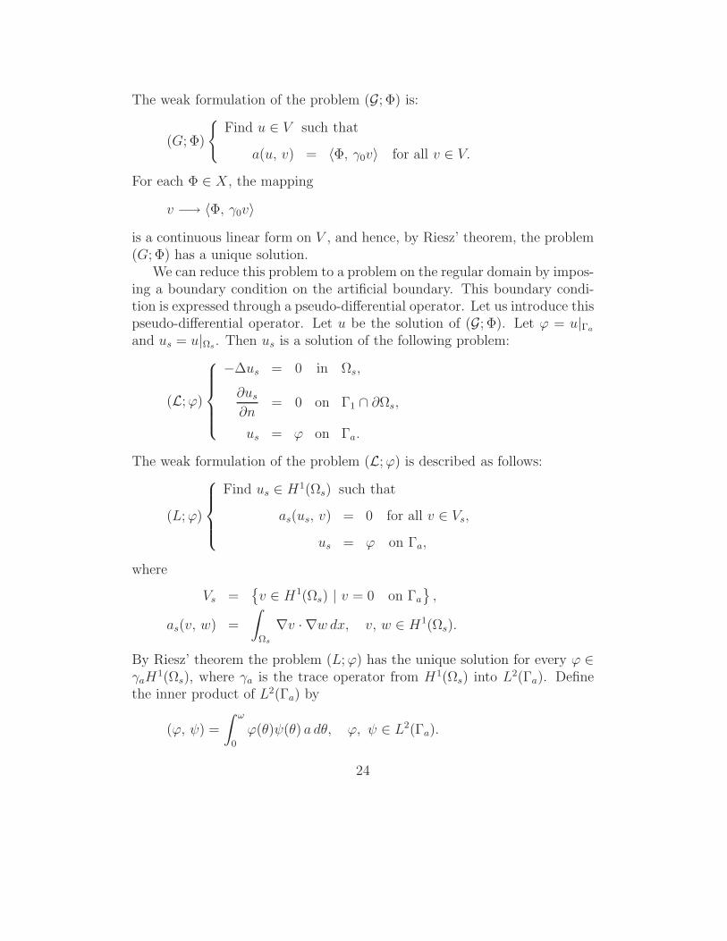
The weak formulation of the problem (G; Φ) is:

(G; Φ)

{Find u ∈ V such that

a(u, v) = 〈Φ, γ0v〉 for all v ∈ V.

For each Φ ∈ X, the mapping

v −→ 〈Φ, γ0v〉

is a continuous linear form on V , and hence, by Riesz’ theorem, the problem(G; Φ) has a unique solution.

We can reduce this problem to a problem on the regular domain by impos-ing a boundary condition on the artificial boundary. This boundary condi-tion is expressed through a pseudo-differential operator. Let us introduce thispseudo-differential operator. Let u be the solution of (G; Φ). Let ϕ = u|Γa

and us = u|Ωs. Then us is a solution of the following problem:

(L; ϕ)

⎧⎪⎪⎪⎨⎪⎪⎪⎩−Δus = 0 in Ωs,

∂us

∂n= 0 on Γ1 ∩ ∂Ωs,

us = ϕ on Γa.

The weak formulation of the problem (L; ϕ) is described as follows:

(L; ϕ)

⎧⎪⎪⎨⎪⎪⎩Find us ∈ H1(Ωs) such that

as(us, v) = 0 for all v ∈ Vs,

us = ϕ on Γa,

where

Vs ={v ∈ H1(Ωs) | v = 0 on Γa

},

as(v, w) =

∫Ωs

∇v · ∇w dx, v, w ∈ H1(Ωs).

By Riesz’ theorem the problem (L; ϕ) has the unique solution for every ϕ ∈γaH

1(Ωs), where γa is the trace operator from H1(Ωs) into L2(Γa). Definethe inner product of L2(Γa) by

(ϕ, ψ) =

∫ ω

0

ϕ(θ)ψ(θ) a dθ, ϕ, ψ ∈ L2(Γa).

24

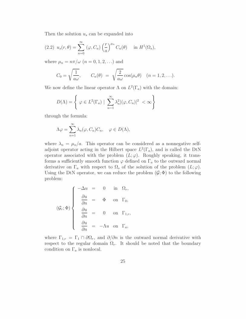
Then the solution us can be expanded into

(2.2) us(r, θ) =∞∑

n=0

(ϕ, Cn)(r

a

)μn

Cn(θ) in H1(Ωs),

where μn = nπ/ω (n = 0, 1, 2, . . .) and

C0 =

√1

aω, Cn(θ) =

√2

aωcos(μnθ) (n = 1, 2, . . .).

We now define the linear operator Λ on L2(Γa) with the domain:

D(Λ) =

{ϕ ∈ L2(Γa) |

∞∑n=1

λ2n|(ϕ, Cn)|2 < ∞

}through the formula:

Λϕ =∞∑

n=1

λn(ϕ, Cn)Cn, ϕ ∈ D(Λ),

where λn = μn/a. This operator can be considered as a nonnegative self-adjoint operator acting in the Hilbert space L2(Γa), and is called the DtNoperator associated with the problem (L; ϕ). Roughly speaking, it trans-forms a sufficiently smooth function ϕ defined on Γa to the outward normalderivative on Γa with respect to Ωs of the solution of the problem (L; ϕ).Using the DtN operator, we can reduce the problem (G; Φ) to the followingproblem:

(Gr; Φ)

⎧⎪⎪⎪⎪⎪⎪⎪⎪⎪⎨⎪⎪⎪⎪⎪⎪⎪⎪⎪⎩

−Δu = 0 in Ωr,

∂u

∂n= Φ on Γ0,

∂u

∂n= 0 on Γ1,r,

∂u

∂n= −Λu on Γa,

where Γ1,r = Γ1 ∩ ∂Ωr , and ∂/∂n is the outward normal derivative withrespect to the regular domain Ωr. It should be noted that the boundarycondition on Γa is nonlocal.

25

Now we define, for each s ≥ 0, the fractional power Λs, of Λ, with thedomain:

D(Λs) =

{ϕ ∈ L2(Γa) |

∞∑n=1

λ2sn |(ϕ, Cn)|2 < ∞

}

through the formula:

Λsϕ =∞∑

n=1

λsn(ϕ, Cn)Cn, ϕ ∈ D(Λs).

Then D(Λs) is a Hilbert space equipped with the norm ‖ϕ‖s,Γa = {(ϕ, ϕ) +(Λsϕ, Λsϕ)}1/2. We shall use the semi-norm |ϕ|s,Γa = (Λsϕ, Λsϕ)1/2.

To pose the weak formulation of the problem (Gr; Φ), we define the bilin-ear form t(·, ·) by

t(v, w) = ar(v, w) + l(γav, γaw), v, w ∈ H1(Ωr),

where

ar(v, w) =

∫Ωr

∇v · ∇w dx, v, w ∈ H1(Ωr),

l(ϕ, ψ) = (Λ1/2ϕ, Λ1/2ψ) =

∞∑n=1

λn(ϕ, Cn)(ψ, Cn), ϕ, ψ ∈ D(Λ1/2),

and we also denote by γa the trace operator from H1(Ωr) into L2(Γa). Thebilinear form t(·, ·) is well defined because of the relation

(2.3) D(Λ1/2) = γaH1(Ωr).

This relation follows from the fact that D(Λ1/2) = γaH1(Ωs) (see [127]) and

(2.4) γaH1(Ωr) = γaH

1(Ωs).

The equality (2.4) follows from the continuation theorem (e.g., Theorem1.4.3.1 of Grisvard [59], Theorem 3.9 of Necas [110]) since each of the bound-aries of Ωr and Ωs is a Lipschitz boundary. We next define

Vr =

{v ∈ H1(Ωr) |

∫Γ0

γ0v dγ = 0

},

26

where we also denote by γ0 the trace operator from H1(Ωr) into L2(Γ0). Sincethe inequality (2.1), replaced Ω, and a(·, ·), with Ωr, and ar(·, ·), respectively,also holds good, we have

(2.5) ‖v‖1,Ωr ≤ C(Ωr)|v|1,Ωr

for all v ∈ Vr. This implies that Vr is a Hilbert space equipped with the innerproduct ar(·, ·). We can now describe the weak formulation of the problem(Gr; Φ) as follows:

(Gr; Φ)

{Find u ∈ Vr such that

t(u, v) = 〈Φ, γ0v〉 for all v ∈ Vr.

This problem has the unique solution for every Φ ∈ X since the bilinear formt(·, ·) is coercive on Vr: t(v, v) ≥ |v|21,Ωr

for all v ∈ Vr.We can now see that (G; Φ) is equivalent to (Gr; Φ). Namely, we can

state the following proposition.

Proposition 2.1 For each Φ ∈ X, let u be the solution of (G; Φ). Letur = u|Ωr and us = u|Ωs. Then ur is the solution of the problem (Gr; Φ), andus can be expressed in the following form:

us(r, θ) =∞∑

n=0

(u|Γa, Cn)(r

a

)μn

Cn(θ) in Ωs.

Conversely, let ur be the solution of (Gr; Φ) and let

u =

⎧⎪⎪⎨⎪⎪⎩ur in Ωr,

∞∑n=0

(γaur, Cn)(r

a

)μn

Cn(θ) in Ωs,

then u is the solution of (G; Φ).

A proof of Proposition 2.1 is presented in the authors’ report [93]. In theproof, the following lemma plays an essential role.

Lemma 2.1 For each ϕ ∈ γaH1(Ωs), let u be the solution of (L; ϕ). Then

we have

(2.6) as(u, v) = l(ϕ, γav) for all v ∈ H1(Ωs).

27

Proof. For every ϕ ∈ γaH1(Ωs), let u be the solution of (L; ϕ). For every

v ∈ H1(Ωs), let w be the solution of (L; γav). Then we have v −w ∈ Vs, andhence we get

(2.7) as(u, v) = as(u, w).

Let

Ξn(r, θ) =(r

a

)μn

Cn(θ) (n = 1, 2, . . .),

then we have

as(Ξn, Ξm) = λnδnm (n, m = 1, 2, . . .).

Therefore, it follows easily from (2.2) that

(2.8) as(u, w) =

∞∑n=1

λn(ϕ, Cn)(γav, Cn) = l(ϕ, γav).

From (2.7) and (2.8), we obtain (2.6).

In the same manner as above, we can also reduce the problem (P ) to thefollowing problem:

(Pr)

⎧⎪⎪⎪⎪⎪⎪⎪⎪⎪⎨⎪⎪⎪⎪⎪⎪⎪⎪⎪⎩

−Δu = 0 in Ωr,

∂u

∂n= αu on Γ0,

∂u

∂n= 0 on Γ1,r,

∂u

∂n= −Λu on Γa,

and then we can describe the weak formulation of the problem (Pr) as follows:

(Πr)

{Find {α, u} ∈ R × {H1(Ωr) \ {0}} such that

t(u, v) = α〈γ0u, γ0v〉 for all v ∈ H1(Ωr).

By the same argument as was described in Section 2.1, we can see that (Πr)has a countable sequence of nonnegative eigenvalues. Moreover, we see fromProposition 2.1 that (Π) is equivalent to (Πr).

28

2.3 The discrete approximation problem and

main theorems

In this section we describe how to approximate the eigenvalues and the corre-sponding eigenvectors of (Πr) by using the finite element method, and statemain theorems of this paper, which are concerned with error estimates forapproximate eigenvalues and eigenvectors.

Let W h be a finite dimensional subspace of H1(Ωr). Applying the finiteelement method directly to (Πr), we get the discrete approximation problem:{

Find {αh, uh} ∈ R ×{W h \ {0}

}such that

t(uh, vh) = αh〈γ0uh, γ0v

h〉 for all vh ∈ W h.

However, we can not compute this problem because t(·, ·) involves an infiniteseries. Therefore, to obtain approximate solutions of (Πr), we have to replacethe bilinear form t(·, ·) by the bilinear form tM(·, ·) defined by

tM(v, w) = ar(v, w) + lM(γav, γaw),

where

lM(ϕ, ψ) =

M∑n=1

λn(ϕ, Cn)(ψ, Cn), ϕ, ψ ∈ L2(Γa).

We solve the following discrete approximation problem:

(ΠMhr )

{Find {αMh, uMh} ∈ R ×

{W h \ {0}

}such that

tM(uMh, vh) = αMh〈γ0uMh, γ0v

h〉 for all vh ∈ W h.

Suppose that W h contains the constant functions and that dim γ0Wh =

Nh + 1. Then the problem (ΠMhr ) has nonnegative eigenvalues:

0 = αMh0 < αMh

1 ≤ αMh2 ≤ . . . ≤ αMh

Nh .

When getting an eigenvector uMhr of (ΠMh

r ), we define an approximate eigen-vector in the whole domain Ω through the following formula:

(2.9) uMh =

⎧⎪⎪⎨⎪⎪⎩uMh

r in Ωr,

M∑n=0

(γauMhr , Cn)

(r

a

)μn

Cn(θ) in Ωs.

29

Let{W h| h ∈ (0, h]

}be a family of finite dimensional subspaces of H1(Ωr).

We will hereafter make the following assumption.

Hypothesis 2 The family{W h| h ∈ (0, h]

}satisfies the following condi-

tion:

(H)

{There is a constant C1 such that for each u ∈ H2(Ωr) and h ∈ (0, h],

infwh∈W h

‖u − wh‖1,Ωr ≤ C1h‖u‖2,Ωr .

For every h ∈ (0, h], W h contains the constant functions.

On Assumptions 1 and 2, we can obtain error estimates for the approx-imate eigenvectors, which will be described in Theorems 2.1 and 2.2, andan error estimate for the approximate eigenvalues, which will be describedin Theorem 2.3. To state these theorems, we prepare some notations. Letα1, α2, . . . be the positive eigenvalues of (Π) ordered by increasing magni-tude taking account of multiplicities. For i ∈ N, suppose αki

is a positiveeigenvalue of (Π) with multiplicity qi, i.e., suppose

αki−1 < αki= αki+1 = · · · = αki+qi−1 < αki+qi

= αki+1.

Here ki is the lowest index of the ith distinct positive eigenvalue. LetV (i) be the space of eigenvectors of (Π) corresponding to αki

. For eachi ∈ N, there is hi ∈ (0, h] such that Nh ≥ ki + qi − 1 for all h ∈ (0, hi],where dim γ0W

h = Nh + 1. For all h ∈ (0, hi], V Mhr (i) is the direct

sum of the spaces of eigenvectors of (ΠMhr ) corresponding to the eigenval-

ues {αMhki

, αMhki+1, . . . , αMh

ki+qi−1}. We will hereafter discuss for fixed i ∈ N.

Theorem 2.1 Suppose that the domain Ω satisfies Assumption 1, and thatthe family

{W h| h ∈ (0, h]

}satisfies Assumption 2. Let u1, u2, . . . , uqi

beany orthonormal basis for V (i) with respect to a(·, ·). Then for sufficientlylarge integer M and for sufficiently small h ∈ (0, hi], there is an orthonormalbasis uMh

r,1 , uMhr,2 , . . . , uMh

r,qifor V Mh

r (i) with respect to tM (·, ·) such that ifwe define the approximate eigenvectors uMh

l (l = 1, 2, . . . , qi) in the wholedomain Ω as (2.9), then for each s > 0,

(2.10) |ul − uMhl |1,Ωr + |ul − uMh

l |1,Ωs ≤ CsM−s + Ch (l = 1, 2, . . . , qi),

where Cs and C are constants independent of M and h.

30


{W h| h ∈ (0, h]

}satisfies Assumption 2. For sufficiently large

integer M and for sufficiently small h ∈ (0, hi], let uMhr,1 , uMh

r,2 , . . . , uMhr,qi

be any orthonormal basis for V Mhr (i) with respect to tM (·, ·). We define the

approximate eigenvectors uMhl (l = 1, 2, . . . , qi) in the whole domain Ω as

(2.9). Then there is an orthonormal basis u(Mh)1 , u

(Mh)2 , . . . , u

(Mh)qi for V (i)

with respect to a(·, ·) such that for each s > 0,

|uMhl −u

(Mh)l |1,Ωr + |uMh

l −u(Mh)l |1,Ωs ≤ CsM

−s +Ch (l = 1, 2, . . . , qi),



{W h| h ∈ (0, h]

}satisfies Assumption 2. Let αki

be the ith distinctpositive eigenvalue of (Π) with multiplicity qi. For sufficiently large integerM and for sufficiently small h ∈ (0, hi], let αMh

1 , αMh2 , . . . , αMh

Nh be thepositive eigenvalues of (ΠMh

r ) ordered by increasing magnitude taking accountof multiplicities. Then, for each s > 0,

(2.11) |αki− αMh

ki+l−1| ≤ CsM−s + Ch2 (l = 1, 2, . . . , qi),


Remark 2.2 To construct the family{W h| h ∈ (0, h]

}which satisfies As-

sumption 2, we need to consider curved elements (see Zlamal [144]) sincethe artificial boundary Γa is a circular arc. We can construct such a familyin the following. Let T h be a triangulation of Ωr whose elements are curvedelements near Γa. Every curved element has two vertices b0, b2 on Γa, and

one vertex b1 in Ωr. Its boundary consists of the arc�

b0b2⊂ Γa and of theline segments b0b1 and b1b2 (see Fig. 2.4). Let T h

0 be the set of all curved

elements belonging to T h. Let T be a reference triangle. For each T ∈ T h0 ,

let x : T −→ T be the map defined by (4) of [144]. We define

W h ={vh ∈ C0(Ωr) | vh|T ◦ x ∈ P1(T ) for T ∈ T h

0 ,

vh|T ∈ P1(T ) for T ∈ T h \ T h0

},

where P1(T ) is the set of all polynomials of degree ≤ 1 on T . Then W h ⊂H1(Ωr) and contains the constant functions. Assume a family of triangu-lations {T h | h ∈ (0, h]} is regular in the sense of Ciarlet [21]. Namely,

31

h = maxT∈T h

hT , and there exists a constant σ such that

hT

ρT

≤ σ for all T ∈⋃

0<h≤h

T h.

Here, for every element T with vertices b0, b1, and b2, the quantities hT ,and ρT , are the diameters of the circumscribed, and the inscribed, circles ofthe triangle b0b1b2, respectively. Then, according to Theorem 2 of [144], thefamily

{W h| h ∈ (0, h]

}satisfies the condition (H).

Ω

Γ

1

0

b

a

r

b

b

T2

Figure 2.4: Curved element T .

2.4 Preliminary consideration for error esti-

mate

Lemma 2.2 There exists a constant ζ such that for every v ∈ Vr,

(2.12) |γav|1/2,Γa ≤ ζ |v|1,Ωr.

Proof. Since γa : H1(Ωr) −→ D(Λ1/2) is a closed operator, it follows from(2.3) and the closed graph theorem that γa ∈ L(H1(Ωr), D(Λ1/2)). Hencewe can see from (2.5) that we have (2.12).

32

This lemma implies that the norms ‖ · ‖t (= t(·, ·)1/2) and ‖ · ‖tM (=tM(·, ·)1/2) on Vr are equivalent to | · |1,Ωr , i.e., for all v ∈ Vr,

(2.13) |v|1,Ωr ≤ ‖v‖tM ≤ ‖v‖t ≤ Cζ|v|1,Ωr ,

where Cζ =√

1 + ζ2. From (2.13), it is immediate that

(2.14) ‖v‖t ≤ Cζ‖v‖tM .

We will hereafter take t(·, ·) to be the inner product on Vr.As mentioned in Section 2.2, for every Φ ∈ X, the problem (Gr; Φ) has the

unique solution u. Hence, there is a linear bounded operator Gr : X −→ Vr

such that GrΦ = u.

Lemma 2.3 For each Φ ∈ X, let u be the solution of (Gr; Φ), i.e., u = GrΦ,then γau ∈ D(Λs) for every s ≥ 0. In addition, γaGr ∈ L(X, D(Λs)) foreach s ≥ 0.

Proof. For each Φ ∈ X, let u be the solution of (Gr; Φ). Let ϕ = γau. Wechoose a positive number b such that b > a and b is sufficiently close to a.Let Γb be the artificial boundary with radius b. Let ϕb = u|Γb

and

Cb0 =

√1

bω, Cb

n(θ) =

√2

bωcos μnθ (n = 1, 2, . . .).

Let (·, ·)b denote the inner product of L2(Γb). Then, by Proposition 2.1, wehave

ϕ(θ) =

∞∑n=0

(ϕb, Cbn)b

(a

b

)μn

Cbn(θ).

Hence ϕ is an even function of class C∞, which implies that ϕ ∈ D(Λs) fors ≥ 0.

Further, since γaGr : X −→ D(Λs) is a closed operator, it follows fromthe closed graph theorem that γaGr ∈ L(X, D(Λs)).

2.4.1 Estimate for the truncation error

We define the linear operator Br : Vr −→ Vr such that

t(Bru, v) = 〈γ0u, γ0v〉 for all u, v ∈ Vr.

33

By the same argument as that for B in Section 2.1, we can see that Br is acompact, nonnegative selfadjoint operator on Vr and that the problem (Πr)can be written in the following form:{

Find {β, u} ∈ {R \ {0}} × {Vr \ {0}} such that

Bru = βu in Vr.

Then α is a positive eigenvalue of (Πr) if and only if β = 1/α is a positiveeigenvalue of Br.

Further, we define BMr ∈ L(Vr) such that

tM(BMr u, v) = 〈γ0u, γ0v〉 for all u, v ∈ Vr.

In this subsection, we derive an estimate for ‖Br − BMr ‖L(Vr).

We here define the bilinear form rM(·, ·) by

rM(v, w) =

∞∑n=M+1

λn(γav, Cn)(γaw, Cn) for all v, w ∈ H1(Ωr).

We will write rM(v) instead of rM(v, v)1/2.

Proposition 2.2 Let u be the solution of (Gr; Φ), then for every s ≥ 0,

(2.15) rM(u) ≤ (λM+1)−s|γau|s+1/2,Γa.

Proof. By Lemma 2.3, γau ∈ D(Λs) for all s ≥ 0. Therefore we have

∞∑n=M+1

λn|(γau, Cn)|2

=

∞∑n=M+1

1

λsn

λs+1n |(γau, Cn)|2

≤ (λM+1)−s

( ∞∑n=M+1

λ2s+1n |(γau, Cn)|2

)1/2( ∞∑n=M+1

λn|(γau, Cn)|2)1/2

.

This yields (2.15).

We next define QM ∈ L(Vr) through the following identity:

tM(QMu, v) = t(u, v) for all u, v ∈ Vr.

34

Then we have

(2.16) BMr = QMBr,

and

(2.17) tM((I − QM)u, v) = −rM(u, v) for all u, v ∈ Vr.

Proposition 2.3 For each s > 0, there is a constant Cs independent of Msuch that

(2.18) ‖Br − BMr ‖L(Vr) ≤ Cs(λM+1)

−s.

Proof. Step 1. There is a constant C ′ independent of M such that for everyv ∈ Vr,

(2.19) ‖(I − QM )v‖t ≤ C ′rM(v).

Indeed, from (2.14) and (2.17), we have

‖(I − QM)v‖2t ≤ C2

ζ ‖(I − QM )v‖2tM

= −C2ζ rM(v, (I − QM)v)

≤ C2ζ r

M(v)‖(I − QM)v‖t.

This shows (2.19).Step 2. For each s > 0, there is a constant C ′′

s independent of M suchthat for every v ∈ Vr,

(2.20) rM(Brv) ≤ C ′′s (λM+1)

−s‖v‖t.

In fact, we have γaBr = γaGrγ0. Hence, it follows from Lemma 2.3 that wehave γaBr ∈ L(Vr, D(Λs+1/2)). Furthermore, from Proposition 2.2, we get

rM(Brv) ≤ (λM+1)−s‖γaBrv‖s+1/2,Γa

≤ (λM+1)−s‖γaBr‖L(Vr , D(Λs+1/2))‖v‖t.

Thus we see that (2.20) holds.Step 3. It follows from (2.16), (2.19), and (2.20) that for every v ∈ Vr,

(2.21) ‖(Br−BMr )v‖t = ‖(I−QM )Brv‖t ≤ C ′rM(Brv) ≤ C ′C ′′

s (λM+1)−s‖v‖t.

From (2.21), we can obtain (2.18).

35

2.4.2 Estimate for the discretization error

As mentioned in Section 2.3, we assume that the family{W h| h ∈ (0, h]

}of finite dimensional subspaces of H1(Ωr) satisfies Assumption 2. Let V h =W h ∩ Vr (0 < h ≤ h). Then we see that the family

{V h| h ∈ (0, h]

}satisfies

the following condition:

(H ′)

{There is a constant C ′

1 such that for each u ∈ H2(Ωr) ∩ Vr and

h ∈ (0, h], infvh∈V h

‖u − vh‖1,Ωr ≤ C ′1h‖u‖2,Ωr .

In addition, if dim γ0Wh = Nh + 1, then we have dim γ0V

h = Nh.We define the linear operator BMh

r : Vr −→ V h such that

tM(BMhr u, vh) = 〈γ0u, γ0v

h〉 for all u ∈ Vr and for all vh ∈ V h.

Then, since BMhr is an operator of finite rank on Vr, BMh

r is a compactoperator on Vr. The spectrum σ(BMh

r ) of BMhr consists of zero and positive

eigenvalues:

βMh1 ≥ βMh

2 ≥ · · · ≥ βMhNh ,

i.e., σ(BMhr ) = {0} ∪ {βMh

i }Nh

i=1. Then zero is an eigenvalue of BMhr . Note

that αMh is a positive eigenvalue of (ΠMhr ) if and only if βMh = 1/αMh is a

positive eigenvalue of BMhr . Hence we can write (ΠMh

r ) in the following form:{Find {βMh, uMh} ∈ {R \ {0}} × {Vr \ {0}} such that

BMhr uMh = βMhuMh.

We will derive an estimate for ‖BMr −BMh

r ‖L(Vr) under the condition (H ′).Now, let P Mh : Vr −→ V h be the orthogonal projection with respect to

tM(·, ·), then we have

(2.22) BMhr = P MhBM

r .

Proposition 2.4 For each s > 0, we have

(2.23) ‖BMr − BMh

r ‖L(Vr) ≤ Cs(λM+1)−s + Ch,


36

Proof. By (2.22), (2.14), and (2.13), we have, for every v ∈ Vr,

‖BMr v − BMh

r v‖t(2.24)

= ‖(I − P Mh)BMr v‖t

≤ Cζ‖(I − P Mh)BMr v‖tM

= Cζ infvh∈V h

‖BMr v − vh‖tM

≤ Cζ

{‖(Br − BM

r )v‖tM + infvh∈V h

‖Brv − vh‖tM

}≤ Cζ

{‖(Br − BM

r )v‖t + Cζ infvh∈V h

‖Brv − vh‖1,Ωr

}.

We here note that

(2.25) Br ∈ L(Vr, H2(Ωr)).

In fact, for every v ∈ Vr, Brv is the solution of the problem (Gr; γ0v). Hence,we can see from Proposition 2.1 that Brv can be extended into Ω such thatit is the solution of the problem (G; γ0v). This implies that by Assumption 1we have Brv ∈ H2(Ωr) (see [59], [60]). Therefore, applying the closed graphtheorem, we obtain (2.25).

From (2.24), (2.25), (H ′), and Proposition 2.3, we have

‖BMr v − BMh

r v‖t

≤ Cζ

{‖Br − BM

r ‖L(Vr)‖v‖t + CζC′1h‖Br‖L(Vr , H2(Ωr))‖v‖t

}≤ Cζ

{Cs(λM+1)

−s + CζC′1h‖Br‖L(Vr , H2(Ωr))

}‖v‖t.

This implies (2.23).

2.5 Proof of the main theorems

In this section, we prove the theorems described in Section 2.3.We first note that as a consequence of Propositions 2.3 and 2.4, we get

the following proposition.

Proposition 2.5 For each s > 0, we have

‖Br − BMhr ‖L(Vr) ≤ Cs(λM+1)

−s + Ch,


37

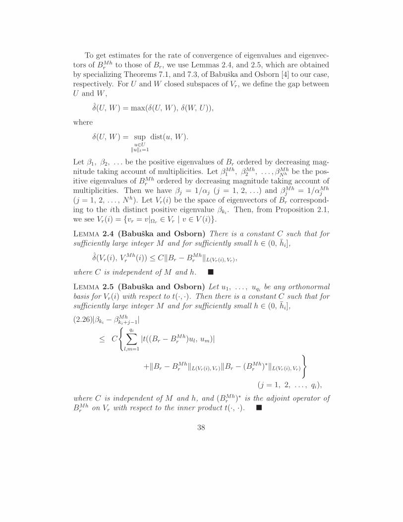
To get estimates for the rate of convergence of eigenvalues and eigenvec-tors of BMh

r to those of Br, we use Lemmas 2.4, and 2.5, which are obtainedby specializing Theorems 7.1, and 7.3, of Babuska and Osborn [4] to our case,respectively. For U and W closed subspaces of Vr, we define the gap betweenU and W ,

δ(U, W ) = max(δ(U, W ), δ(W, U)),

where

δ(U, W ) = supu∈U

‖u‖t=1

dist(u, W ).

Let β1, β2, . . . be the positive eigenvalues of Br ordered by decreasing mag-nitude taking account of multiplicities. Let βMh

1 , βMh2 , . . . , βMh

Nh be the pos-itive eigenvalues of BMh

r ordered by decreasing magnitude taking account ofmultiplicities. Then we have βj = 1/αj (j = 1, 2, . . .) and βMh

j = 1/αMhj

(j = 1, 2, . . . , Nh). Let Vr(i) be the space of eigenvectors of Br correspond-ing to the ith distinct positive eigenvalue βki

. Then, from Proposition 2.1,we see Vr(i) = {vr = v|Ωr ∈ Vr | v ∈ V (i)}.

Lemma 2.4 (Babuska and Osborn) There is a constant C such that forsufficiently large integer M and for sufficiently small h ∈ (0, hi],

δ(Vr(i), V Mhr (i)) ≤ C‖Br − BMh

r ‖L(Vr(i), Vr),

where C is independent of M and h.

Lemma 2.5 (Babuska and Osborn) Let u1, . . . , uqibe any orthonormal

basis for Vr(i) with respect to t(·, ·). Then there is a constant C such that forsufficiently large integer M and for sufficiently small h ∈ (0, hi],

|βki− βMh

ki+j−1|(2.26)

≤ C

{qi∑

l,m=1

|t((Br − BMhr )ul, um)|

+‖Br − BMhr ‖L(Vr(i), Vr)‖Br − (BMh

r )∗‖L(Vr(i), Vr)

}(j = 1, 2, . . . , qi),

where C is independent of M and h, and (BMhr )∗ is the adjoint operator of

BMhr on Vr with respect to the inner product t(·, ·).

38

In addition, to prove Theorem 2.1, we quote Proposition 4.1 of Fu [38],and Lemma 3.4 of Bramble and Osborn [14], as Lemmas 2.6, and 2.7, respec-tively, and note Remark 2.3.

Lemma 2.6 (Fu) Let E be an inner product space, and let e1, e2, . . . , em

be mutually orthonormal in E. Suppose f1, f2, . . . , fm are elements of Esatisfying

m∑j=1

‖fj − ej‖ < 1,

where ‖ · ‖ denotes the norm of E. Then {f1, f2, . . . , fm} forms a linearlyindependent set.

Lemma 2.7 (Bramble and Osborn) Let E be an inner product space withinner product (·, ·) and norm ‖ · ‖. Let m be a positive integer. There is aconstant Cm such that for f1, f2, . . . , fm any linearly independent set in Eand g1, g2, . . . , gm the corresponding Gram-Schmidt orthonormalization, wehave

max1≤j≤m

‖fj − gj‖ ≤ Cm max1≤j, k≤m

|(fj, fk) − δjk|.

Remark 2.3 Let u be an eigenvector of (Π). Then, by Lemma 2.1, we have

a(u, v) = t(u, v)

for all v ∈ H1(Ω). In addition, let uMhr be an eigenvector of (ΠMh

r ), and letuMh be the approximate eigenvector in Ω defined by (2.9). Then, by Lemma2.1, we also have

ar(uMh, v) + as(u

Mh, v) = tM (uMh, v)

for all v ∈ H1(Ω).

Proof of Theorem 2.1. Let u1, u2, . . . , uqibe any basis for V (i) such that

a(ul, um) = δlm.Step 1. In this step, we show that there exists a basis uMh

r,1 , uMhr,2 , . . . , uMh

r,qi

for V Mhr (i) such that tM(uMh

r,l , uMhr,m) = δlm and

(2.27) |ul − uMhr,l |1,Ωr ≤ CsM

−s + Ch (l = 1, 2, . . . , qi),

39

where Cs and C are constants independent of M and h.According to Remark 2.3, we have

t(ul, um) = a(ul, um) = δlm.

Let EMh : Vr −→ V Mhr (i) be the orthogonal projection with respect to

tM(·, ·), and let vMhl = EMhul (l = 1, 2, . . . , qi).

Step 1.1. For each s > 0, we have

(2.28) ‖ul − vMhl ‖tM ≤ C(1)

s (λM+1)−s + C(2)h (l = 1, 2, . . . , qi).

Indeed, we have

‖ul − vMhl ‖tM ≤ inf

vh∈V Mhr (i)

‖ul − vh‖t ≤ δ(Vr(i), V Mhr (i)),

and hence, by Lemma 2.4, we have

‖ul − vMhl ‖tM ≤ C‖Br − BMh

r ‖L(Vr(i), Vr).

From this inequality and Proposition 2.5, we get (2.28).Step 1.2. From (2.14) and (2.28), if M is sufficiently large and if h is

sufficiently small, then we have

qi∑l=1

‖ul − vMhl ‖t < 1.

Then Lemma 2.6 implies that vMhl (l = 1, 2, . . . , qi) are mutually linearly

independent.Step 1.3. Let

{uMh

r,l

}qi

l=1be the Gram-Schmidt orthonormalization of{

vMhl

}qi

l=1with respect to tM (·, ·). Then we show

(2.29) ‖vMhl − uMh

r,l ‖t ≤ C(3)

[max1≤l≤qi

‖ul − vMhl ‖t + max

1≤l≤qi

{rM(ul)

}2]

.

In fact, it follows from (2.14) and Lemma 2.7 that for l = 1, 2, . . . , qi,

(2.30) ‖vMhl − uMh

r,l ‖t ≤ CζCqimax

1≤l, m≤qi

|tM(vMhl , vMh

m ) − δlm|.

In addition, since t(ul, um) = δlm,

|tM(vMhl , vMh

m ) − δlm| = |tM(vMhl , vMh

m ) − t(ul, um)|(2.31)

= |tM(vMhl , um) − tM (ul, um) − rM(ul, um)|

≤ ‖vMhl − ul‖t + rM(ul)r

M(um).

40

Combining (2.30) and (2.31), we get (2.29).Step 1.4. From (2.29), we have, for l = 1, 2, . . . , qi,

‖ul − uMhr,l ‖t ≤ ‖ul − vMh

l ‖t + ‖vMhl − uMh

r,l ‖t(2.32)

≤ (C(3) + 1) max1≤l≤qi

‖ul − vMhl ‖t + C(3) max

1≤l≤qi

{rM(ul)

}2.

By Proposition 2.2, we have, for each s > 0,

(2.33) rM(ul) ≤ (λM+1)−s‖γa‖L(Vr(i), D(Λs+1/2))‖ul‖t (l = 1, 2, . . . , qi).

From (2.32), (2.28), and (2.33), we see that (2.27) holds good.Step 2. Let uMh

s,1 , uMhs,2 , . . . , uMh

s,qibe the approximate eigenvectors on Ωs

defined by (2.9). In this step, we show that there exist constants Cs and Cindependent of M and h such that

(2.34) |ul − uMhs,l |1,Ωs ≤ CsM

−s + Ch (l = 1, 2, . . . , qi).

By Lemmas 2.1 and 2.2, we have, for l = 1, 2, . . . , qi,

|ul − uMhs,l |21,Ωs

=

M∑n=1

λn

∣∣(γa(ul − uMhr,l ), Cn)

∣∣2 +

∞∑n=M+1

λn |(γaul, Cn)|2

≤ ζ2∣∣ul − uMh

r,l

∣∣21,Ωr

+ rM(ul)2.

Hence we see from (2.33) that for every s > 0,

(2.35) |ul − uMhs,l |21,Ωs

≤ ζ2∣∣ul − uMh

r,l

∣∣21,Ωr

+ (λM+1)−2s‖γa‖2

L(Vr(i), D(Λs+1/2)).

From (2.35) and (2.27), we obtain (2.34).Step 3. It follows from (2.27) and (2.34) that (2.10) holds good.

We can also prove Theorem 2.2 in a similar fashion, and here omit itsproof, which is described in [93].

Proof of Theorem 2.3. We prove Theorem 2.3 by using Lemma 2.5. Letu1, u2, . . . , uqi

be any basis for Vr(i) such that t(ul, um) = δlm.Step 1. In this step, we show that we can estimate the first term on the

right-hand side of (2.26) as follows:qi∑

l,m=1

|t((Br − BMhr )ul, um)|(2.36)

≤ C(1)‖γa‖2L(Vr(i), D(Λs+1/2))(λM+1)

−2s + C(2)‖BMr − BMh

r ‖2L(Vr)

41

for every s > 0. To show (2.36), we first note that we have

qi∑l,m=1

|t((Br − BMhr )ul, um)|(2.37)

≤qi∑

l,m=1

{|t((Br − BM

r )ul, um)| + |t((BMr − BMh

r )ul, um)|}

.

Step 1.1. We show that for each s > 0 and for every l, m = 1, 2, . . . , qi,we have

(2.38) |t((Br − BMr )ul, um)| ≤ C(3)‖γa‖2

L(Vr(i), D(Λs+1/2))(λM+1)−2s.

In fact, by (2.16), we have

(2.39) t((Br − BMr )ul, um) = βki

t((I − QM)ul, um).

Noting that

t((I − QM )ul, um)

= −tM((I − QM)ul, (I − QM )um) + tM((I − QM )ul, um),

we see from (2.17) and (2.19) that

t((I − QM )ul, um)(2.40)

≤ ‖(I − QM)ul‖tM‖(I − QM )um‖tM + |rM(ul, um)|≤ ((C(4))2 + 1)rM(ul)r

M(um),

where C(4) is the constant introduced in (2.19). Hence, from (2.39), (2.40),and (2.33), we get (2.38).

Step 1.2. For every l, m = 1, 2, . . . , qi, we have

(2.41) |t((BMr − BMh

r )ul, um)| ≤ 1

βki

‖BMr − BMh

r ‖2L(Vr).

42

The reason for this inequality is the following. By (2.22) and (2.16), we have

t((BMr − BMh

r )ul, um) = t((I − P Mh)BMr ul, um)

=1

βki

t((I − P Mh)BMr ul, Brum)

=1

βki

tM((I − P Mh)BMr ul, QMBrum)

=1

βki

tM((I − P Mh)BMr ul, (I − P Mh)BM

r um)

≤ 1

βki

‖BMr − BMh

r ‖2L(Vr).

Step 1.3. From (2.37), (2.38), and (2.41), we obtain (2.36).Step 2. We can estimate the second term on the right-hand side of (2.26)

as follows:

‖Br − BMhr ‖L(Vr(i), Vr)‖Br − (BMh

r )∗‖L(Vr(i), Vr)(2.42)

≤ ‖Br − BMhr ‖L(Vr)‖(Br − BMh

r )∗‖L(Vr)

= ‖Br − BMhr ‖2

L(Vr).

Step 3. From (2.26), (2.36), and (2.42), it follows that

|βki− βMh

ki+j−1|≤ C(1)‖γa‖2

L(Vr(i), D(Λs+1/2))(λM+1)−2s + C(2)‖BM

r − BMhr ‖2

L(Vr)

+C(5)‖Br − BMhr ‖2

L(Vr)

for j = 1, 2, . . . , qi. Hence, using Propositions 2.4 and 2.5, we have thevalidity of (2.11).

2.6 Numerical results

To carry out numerical experiments, we chose a water region Ω and a watersurface Γ0 as follows:

Ω = {(x1, x2) | − 2 < x1 < 3, −2 < x2 < 0} \ S

and

Γ0 = {(x1, 0) | − 2 < x1 < 0, 0 < x1 < 3},

43

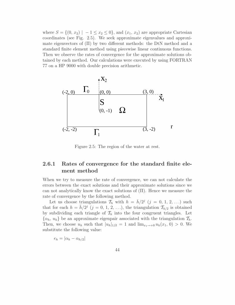
where S = {(0, x2) | − 1 ≤ x2 ≤ 0}, and (x1, x2) are appropriate Cartesiancoordinates (see Fig. 2.5). We seek approximate eigenvalues and approxi-mate eigenvectors of (Π) by two different methods: the DtN method and astandard finite element method using piecewise linear continuous functions.Then we observe the rates of convergence for the approximate solutions ob-tained by each method. Our calculations were executed by using FORTRAN77 on a HP 9000 with double precision arithmetic.

Ω

Γ1

0

x

r

Sx

2

Γ1

(-2, 0) (0, 0) (3, 0)

(-2, -2) (3, -2)

(0, -1)

Figure 2.5: The region of the water at rest.

2.6.1 Rates of convergence for the standard finite ele-

ment method

When we try to measure the rate of convergence, we can not calculate theerrors between the exact solutions and their approximate solutions since wecan not analytically know the exact solutions of (Π). Hence we measure therate of convergence by the following method.

Let us choose triangulations Th with h = h/2j (j = 0, 1, 2, . . .) suchthat for each h = h/2j (j = 0, 1, 2, . . .), the triangulation Th/2 is obtainedby subdividing each triangle of Th into the four congruent triangles. Let{αh, uh} be an approximate eigenpair associated with the triangulation Th.Then, we choose uh such that |uh|1,Ω = 1 and limx1→+0 uh(x1, 0) > 0. Wesubstitute the following value:

eh = |αh − αh/2|

44

for the error between the approximate eigenvalue αh and the exact eigenvalue.We likewise calculate

eh = |uh − uh/2|1,Ω

as a substitute for the error of the approximate eigenvector. This method ofmeasurement is based on the study of Kurata and Ushijima [96], where theydiscussed the adequacy of this method.

We adopted the triangulation shown in Fig. 2.6 as an initial triangula-tion Th. Rates of convergence for approximate eigenvalues, and approximateeigenvectors, are shown in Figs. 6, and 7, respectively. The lines in thosefigures are the graphs of the linear functions y = px+q which are least squareapproximations to the data of the errors eh and the mesh lengths h which areplotted in log-log scale. In the figures, m denotes a modal number, and thegradient p of each line is written in parentheses. These figures show that form = 1, 2, the rates of convergence for the approximate solutions are slowerthan those expected in the case when the domain is a convex polygon. Thisresult suggests that the eigenvectors of the first and second modes do notbelong to H2(Ω).

Figure 2.6: A triangulation of the water region.

45

2.6.2 Rates of convergence for the DtN finite elementmethod

In practical computations, we approximate the artificial boundary by using apolygonal line since the artificial boundary is a circular arc. We consider thepolygonal line ΓK

a which consists of K equal line segments. Let ΩK denote the

polygonal domain bounded by ΓKa and ∂Ωr \ Γa. The domain ΩK is divided

into triangles. Then, assume that every nodal point on ΓKa is a vertex of ΓK

a

(see Fig. 2.9). We seek approximate solutions by a finite element methodusing piecewise linear continuous functions.

By the same method as was mentioned in the previous subsection, wemeasure rates of convergence for the DtN method. Then we need to payattention to the subdivision of triangles having two vertices on Γa. Let b0,b1, and b2 be the vertices of such a triangle. We subdivide the triangle b0b1b2

into the four triangles shown in Fig. 2.11, where the point b′1 is the midpoint

of the circular arc�

b0b2, and the points b′0, and b′2, are the midpoints of theline segments b1b2, and b0b1, respectively.

We adopted the triangulation shown in Fig. 2.9 as an initial triangulation.When computing the bilinear form lM , we chose M such that M = K, whereK is the number of the division of the artificial boundary. As substitutes forerrors between exact solutions and their approximate solutions, we calculatethe following values:

|α2M2K − αM

K |,{|u2M

2K − uMK |2

1,bΩ2K+ |u2M

2K − uMK |21,Ωs

}1/2

,

where {αMK , uM

K } is an approximate eigenpair associated with a triangulation

of ΩK , and

uMK (r, θ) =

M∑n=0

(K+1∑j=1

uMK (bj)ϕj, Cn

)(r

a

)μn

Cn(θ) in Ωs,

where bj (j = 1, 2, . . . , K + 1) denote the nodal points on Γa, and ϕj (j =1, 2, . . . , K + 1) are piecewise linear continuous functions on Γa satisfyingϕj(bk) = δjk. Then we choose uM

K such that

{|uMK |2

1,bΩK+ |uM

K |21,Ωs}1/2 = 1 and lim

x1→+0uM

K (x1, 0) > 0.

Rates of convergence for approximate eigenvalues, and approximate eigen-vectors, are shown in Figs. 10, and 11, respectively. Comparing these figures

46

with Figs. 6 and 7, we see that for m = 1, 2, the rate of convergence forthe DtN method is better than that for the standard finite element method.When M−1 is proportional to the mesh length h, (2.11) with s = 2 predictsthat the rate of convergence for the approximate eigenvalue is h2, and (2.10)with s = 1 predicts that the rate of convergence for the approximate eigen-vector in the energy norm is h1. The numerical results are consistent withour theoretical results, although in our theoretical analysis, we do not takeaccount of the effect of the approximation of the artificial boundary. Thenumerical results suggest that the approximation of the artificial boundarymentioned above does not deteriorate the rates of convergence in comparisonwith those stated in our theorems. However it has not been theoreticallyanalyzed yet.

2.7 Conclusions

We have applied the DtN finite element method to the eigenvalue problemof the linear water wave (the sloshing problem) in a water region with areentrant corner. We have established error estimates for approximate eigen-values and eigenvectors which imply that the DtN finite element methodimproves the rates of convergence which deteriorate due to the corner singu-larity. Such an improvement was observed the numerical examples in Section2.6.

We can also apply the DtN finite element method to the water waveradiation problem. This topic is investigated in Lenoir–Tounsi [99] for twodimensional case, and in Seto [117] for three dimensional case. Lenoir–Tounsi[99] have derived an error estimate including the truncation error as well asthe discretization error. For the three dimensional problem, such an errorestimate is yet to be established.

47

1e-04

0.001

0.01

0.1

1

0.1 1

erro

r

h

m = 1 (0.993)

m = 2 (1.741)

m = 3 (1.951)

m = 4 (2.015)

Figure 2.7: Convergence behaviors of eigenvalues obtained by the standardfinite element method.

48

0.001

0.01

0.1

1

10

0.1 1

erro

r

h

m = 1 (0.474)

m = 2 (0.848)m = 3 (0.935)

m = 4 (0.942)

Figure 2.8: Convergence behaviors of eigenvectors obtained by the standardfinite element method.

49

Figure 2.9: The polygonal domain ΩK (K = 16) and its triangulation.

Ω

Γ

1

0

b

a

r

b

b

2

b’

b’b’

0

2

1

Figure 2.10: Subdivision of a triangle near the artificial boundary.

50

1e-04

0.001

0.01

0.1

1

0.1 1

erro

r

h

m = 1 (1.979)

m = 2 (1.979)

m = 3 (1.964)

m = 4 (1.987)

Figure 2.11: Convergence behaviors of eigenvalues obtained by the DtN finiteelement method.

51

0.001

0.01

0.1

1

10

0.1 1

erro

r

h

m = 1 (0.967)

m = 2 (0.973)

m = 3 (0.959)

m = 4 (0.950)

Figure 2.12: Convergence behaviors of eigenvectors obtained by the DtNfinite element method.

52

Part II

The Exterior HelmholtzProblem

53

Chapter 3

The DtN Finite ElementMethod

3.1 The exterior Helmholtz problem

We consider the exterior Helmholtz problem:

(3.1)⎧⎪⎪⎨⎪⎪⎩−Δu − k2u = f in Ω,

u = 0 on γ,

limr−→+∞

rd−12

(∂u

∂r− iku

)= 0 (the outgoing radiation condition),

where the wave number k is a positive constant, Ω is an unbounded domainof Rd (d = 2 or 3) with sufficiently smooth boundary γ, f is a given datum,r = |x| for x ∈ Rd, and i =

√−1. Assume that O ≡ Rd \ Ω is a bounded

open set and that f has a compact support.We first introduce a theorem concerning the well-posedness of problem

(3.1).

Theorem 3.1 For every compactly supported f ∈ L2(Ω), problem (3.1) hasa unique solution in H2

loc(Ω), where

Hmloc(Ω) = {u | u ∈ Hm(B) for all bounded open set B ⊂ Ω} (m ∈ N).

Proof. See [112, 115].

54

3.2 The DtN formulation

To reduce the computational domain to a bounded domain, we introduce anartificial boundary Γa = {x ∈ Rd | |x| = a}, where a is a positive numbersuch that O ∪ supp f ⊂ Ba ≡ {x ∈ Rd | |x| < a}. Then the boundedcomputational domain is defined by Ωa = Ω ∩ Ba (see Fig. 3.1), and furtherthe reduced problem is as follows:

(3.2)

⎧⎪⎨⎪⎩−Δu − k2u = f in Ωa,

u = 0 on γ,∂u

∂n= −Su on Γa,

where n is the unit normal vector on Γa, toward infinity, and S is the DtNoperator corresponding to the outgoing radiation condition. The boundarycondition imposed on Γa of (3.2) is called the exact DtN boundary condition.The DtN operator S is defined as follows: for every Dirichlet datum ϕ on Γa,

Γ

Ω

γΟ

a

a

Figure 3.1: Artificial boundary Γa and computational domain Ωa.

Sϕ =∂ue

∂ne

∣∣∣∣Γa

(Neumann datum),

where ne is the unit normal vector on Γa, toward the origin, and ue is thesolution to the following problem:⎧⎪⎪⎨⎪⎪⎩

−Δue − k2ue = 0 in Rd \ Ba,ue = ϕ on Γa,

limr−→∞

rd−12

(∂ue

∂r− ikue

)= 0.

55

We present an analytical representation of the DtN operator. Using ananalytical representation of ue by separation of variables, we can write downthe DtN operator S as follows. In the two-dimensional case,

(3.3) Sϕ(θ) =∞∑

n=−∞−k

H(1)′n (ka)

H(1)n (ka)

ϕnYn(θ),

where θ denotes the angular variable of an (r, θ) polar coordinate system,

H(1)n are the cylindrical Hankel functions of the first kind of order n, the

prime on H(1)n denotes differentiation with respect to the argument, Yn are

the circular harmonics defined by

Yn(θ) =einθ

√2π

and ϕn are the Fourier coefficients defined by

(3.4) ϕn =

∫ 2π

0

ϕ(θ)Yn(θ) dθ.

In the three-dimensional case,

Sϕ(θ, φ) =∞∑

n=0

n∑m=−n

−kh

(1)′n (ka)

h(1)n (ka)

ϕmn Y m

n (θ, φ),

where θ, φ denote the angular variables of an (r, θ, φ) spherical coordinate

system, h(1)n are the spherical Hankel functions of the first kind of order n,

Y mn are the spherical harmonics defined by

Y mn (θ, φ) =

√(2n + 1)

4π

(n − |m|)!(n + |m|)!P

|m|n (cos θ) eimφ,

where P mn are the associated Legendre functions, and ϕm

n are the Fouriercoefficients defined by

(3.5) ϕmn =

∫ 2π

0

dφ

∫ π

0

ϕ(θ, φ)Y mn (θ, φ) sin θ dθ.

Now we define the Sobolev space Hs(Γa) (s > 0) by

Hs(Γa) ={ϕ ∈ L2(Γa) | ‖ϕ‖s,Γa < ∞

},

56

where ‖ · ‖s,Γa is the norm of Hs(Γa) defined by

‖ϕ‖2s,Γa

=

⎧⎪⎪⎪⎪⎪⎪⎨⎪⎪⎪⎪⎪⎪⎩a

∞∑n=−∞

(1 + n2s)|ϕn|2 if d = 2,

a2

∞∑n=0

n∑m=−n

(1 + n2s)|ϕmn |2 if d = 3.

We here note that the DtN operator S is a bounded linear operator fromH1/2(Γa) into H−1/2(Γa) (see [105]), where H−1/2(Γa) is the set of all boundedsemilinear forms on H1/2(Γa).

To formulate a weak form of problem (3.2), we introduce the followingsesquilinear forms:

a(u, v) =

∫Ωa

(∇u · ∇v − k2uv

)dx + s(u, v) for u, v ∈ H1(Ωa),

s(u, v) = 〈Su, v〉H−1/2(Γa)×H1/2(Γa)(3.6)

=

⎧⎪⎪⎪⎪⎪⎪⎨⎪⎪⎪⎪⎪⎪⎩

∞∑n=−∞

−kaH

(1)′n (ka)

H(1)n (ka)

un(a)vn(a) if d = 2,

∞∑n=0

n∑m=−n

−ka2 h(1)′n (ka)

h(1)n (ka)

umn (a)vm

n (a) if d = 3,

where un(a) and umn (a) are the Fourier coefficients of u|Γa defined by (3.4)

and (3.5), respectively. Then a weak form of (3.2) is written as follows: findu ∈ V such that

(3.7) a(u, v) = (f, v)

for all v ∈ V , where

V ={v ∈ H1(Ωa) | v = 0 on γ

},

(u, v) =

∫Ωa

uv dx for u, v ∈ L2(Ωa).

For every f ∈ L2(Ωa), problem (3.7) has a unique solution which is therestriction to Ωa of the solution of problem (3.1) (see [105, 74, 81]).

57

3.3 The DtN finite element method and its

error estimates

We discretize problem (3.7) by using the finite element method to obtainapproximate solutions to problem (3.7) (or (3.1)). We introduce a family{Vh | h ∈ (0, h]} of finite dimensional subspaces of V , and assume that thisfamily satisfies the following condition: there exist an integer p ≥ 2 and aconstant C > 0 such that for all 0 < h ≤ h and for every u ∈ V ∩ Hp′(Ωa)(2 ≤ p′ ≤ p),

(3.8) infvh∈Vh

‖u − vh‖1,Ωa ≤ Chp′−1‖u‖p′,Ωa ,

where C is independent of h and u. For examples of such a family, see[21, 144].

Now since the sesquilinear form s involves the infinite series, we have totruncate it in practice. So we practically solve the following problem: finduN

h ∈ Vh such that

(3.9) aN (uNh , vh) = (f, vh) for all vh ∈ Vh,

where, for N ∈ N,

aN(u, v) =

∫Ωa

(∇u · ∇v − k2uv

)dx + sN(u, v) for u, v ∈ H1(Ωa),

sN(u, v) =

⎧⎪⎪⎪⎪⎪⎪⎨⎪⎪⎪⎪⎪⎪⎩

∑|n|<N

−kaH

(1)′n (ka)

H(1)n (ka)


N−1∑n=0

n∑m=−n

−ka2 h(1)′n (ka)

h(1)n (ka)

umn (a)vm

n (a) if d = 3.

Theorem 3.2 Let k be an arbitrary positive number and f an arbitraryfunction of L2(Ω) with compact support. Assume that O ∪ supp f ⊂ Ba0

(a0 < a). Let u be the solution of problem (3.1). Assume that there existsan integer l ≥ 2 such that u ∈ H l(Ωa). Then there exist a γ0 > 0 such thatfor every (h, N) ∈ (0, h] × N satisfying h + N−1 ≤ γ0, problem (3.9) has aunique solution uN

h , and moreover, if d = 2, then we have

‖u − uNh ‖1,Ωa(3.10)

≤ C

(hm−1‖u‖m,Ωa + N−s+1/2

∣∣∣∣∣ H(1)N (ka)

H(1)N (ka0)

∣∣∣∣∣RN(u; s, a0)

),

58

‖u − uNh ‖0,Ωa(3.11)

≤ C(h + N−1)

(hm−1‖u‖m,Ωa + N−s+1/2

∣∣∣∣∣ H(1)N (ka)

H(1)N (ka0)

∣∣∣∣∣RN(u; s, a0)

),

where m = min{p, l}, s is an arbitrary real number ≥ 1/2,

(3.12) RN(u; s, a0) =

⎛⎝a0

∑|n|≥N

n2s|un(a0)|2⎞⎠2

,

and positive constants γ0 and C depend on k, a0, and Ωa, but are independentof h, N , s, f , u, and uN

h . If d = 3, then (3.10) and (3.11) hold by replacing

H(1)N by h

(1)N , and (3.12) by

RN(u; s, a0) =

(a2

0

∑n≥N

n∑m=−n

n2s|umn (a0)|2

)2

.

Before starting to prove Theorem 3.2, we introduce the following inequal-ities associated with the trace theorem:

(3.13) ‖v‖m−1/2,Γa ≤ C‖v‖m,Ωa for all v ∈ Hm(Ωa) (m = 1, 2),

where C is a positive constant depending on Ωa, but independent of v, andthe following sesquilinear form on H1(Ωa):

rN(u, v) =

⎧⎪⎪⎪⎪⎪⎪⎨⎪⎪⎪⎪⎪⎪⎩

∑|n|≥N

−kaH

(1)′n (ka)

H(1)n (ka)


∑n≥N

n∑m=−n

−ka2 h(1)′n (ka)

h(1)n (ka)

umn (a)vm

n (a) if d = 3.

Note here that we have

s(u, v) = sN(u, v) + rN(u, v) for u, v ∈ H1(Ωa).

Proof. We prove only in the case when d = 2, because the proof of the casewhen d = 3 is exactly same.

59

We first assume that problem (3.9) has a solution uNh . We postpone

proving the well-posedness of problem (3.9) until completion of the derivationof (3.10) and (3.11).

Set eNh = u − uN

h . Then we have

(3.14) aN(eNh , vh) + rN(u, vh) = 0

for all vh ∈ Vh. Note the following identical equation:

‖eNh ‖2

1,Ωa= aN(eN

h , eNh ) + (k2 + 1)‖eN

h ‖20,Ωa

− sN (eNh , eN

h ).

Taking the real part of this identity, we can get

‖eNh ‖2

1,Ωa= Re

{aN(eN

h , eNh )}

+ (k2 + 1)‖eNh ‖2

0,Ωa− Re

{sN(eN

h , eNh )}

.

By virtue of Lemma A.1, we have

(3.15) ‖eNh ‖2

1,Ωa≤ Re

{aN (eN

h , eNh )}

+ (k2 + 1)‖eNh ‖2

0,Ωa.

Step 1. We show that for an arbitrary ε > 0, there exists a positiveconstant C3(ε) such that

|aN(eNh , eN

h )|(3.16)

≤ ε‖eNh ‖2

1,Ωa

+C3(ε)

⎧⎨⎩h2m−2‖u‖2m,Ωa

+ N−2s+1

∣∣∣∣∣ H(1)N (ka)

H(1)N (ka0)

∣∣∣∣∣2 [

RN(u; s, a0)]2⎫⎬⎭ ,

where s is an arbitrary number ≥ 1/2 and C3(ε) depends on k, a0, and Ωa,but is independent of h, N , s, u, and uN

h . By (3.14), we have, for all vh ∈ Vh,

aN(eNh , eN

h ) = aN (eNh , u − vh) + rN(u, uN

h − vh)

= aN (eNh , u − vh) + rN(u, u − vh) − rN(u, eN

h ).

Thus, by using the trigonometric inequality, the Schwarz inequality, LemmaA.6, and the trace inequality (3.13), we get

|aN(eNh , eN

h )| ≤ |eNh |1,Ωa |u − vh|1,Ωa + k2‖eN

h ‖0,Ωa‖u − vh‖0,Ωa(3.17)

+C(k, a)‖eNh ‖1/2,Γa‖u − vh‖1/2,Γa

+|rN(u, u − vh)| + |rN(u, eNh )|

≤ C(k, Ωa)‖eNh ‖1,Ωa‖u − vh‖1,Ωa

+|rN(u, u − vh)| + |rN(u, eNh )|.

60

Let us estimate the second term on the right-hand side of (3.17). SinceO ∪ supp f ⊂ Ba0 , the solution u can be analytically represented as follows:

u(r, θ) =

∞∑n=−∞

H(1)n (kr)

H(1)n (ka0)

un(a0)Yn(θ) on R2 \ Ba0 .

This implies

un(a) =H

(1)n (ka)

H(1)n (ka0)

un(a0)

for all n ∈ Z. Moreover, we can see from the usual regularity argument thatu|Γa0

∈ Hs(Γa0) for all s > 0. Thus, by the trigonometric inequality, LemmasA.6 and A.7, the Schwarz inequality, and the trace inequality (3.13), we have,for every s ≥ 1/2,

|rN(u, u − vh)|(3.18)

≤∑|n|≥N

∣∣∣∣∣kaH

(1)′n (ka)

H(1)n (ka)

∣∣∣∣∣ |un(a)||(u − vh)n(a)|

=∑|n|≥N

|n|−s+1/2

∣∣∣∣∣ka

n

H(1)′n (ka)

H(1)n (ka)

∣∣∣∣∣∣∣∣∣∣ H(1)

n (ka)

H(1)n (ka0)

∣∣∣∣∣ |n|s|un(a0)||n|1/2|(u − vh)n(a)|

≤ C(k, a, a0)N−s+1/2

∣∣∣∣∣ H(1)N (ka)

H(1)N (ka0)

∣∣∣∣∣RN(u; s, a0)‖u − vh‖1/2,Γa

≤ C(k, a0, Ωa)N−s+1/2

∣∣∣∣∣ H(1)N (ka)

H(1)N (ka0)

∣∣∣∣∣RN(u; s, a0)‖u − vh‖1,Ωa,

where (u − vh)n(a) are the Fourier coefficients of u − vh. In exactly thesame way, we can estimate the third term on the right-hand side of (3.17) asfollows:

(3.19) |rN(u, eNh )| ≤ C(k, a0, Ωa)N

−s+1/2

∣∣∣∣∣ H(1)N (ka)

H(1)N (ka0)

∣∣∣∣∣RN (u; s, a0)‖eNh ‖1,Ωa .

61

Combining (3.17), (3.18), (3.19), and (3.8) leads to

|aN(eNh , eN

h )| ≤ C(k, a0, Ωa)

[hm−1‖eN

h ‖1,Ωa‖u‖m,Ωa

+hm−1N−s+1/2

∣∣∣∣∣ H(1)N (ka)

H(1)N (ka0)

∣∣∣∣∣RN(u; s, a0)‖u‖m,Ωa

+N−s+1/2

∣∣∣∣∣ H(1)N (ka)

H(1)N (ka0)

∣∣∣∣∣ ‖eNh ‖1,ΩaR

N(u; s, a0)

].

Applying the arithmetic-geometric mean inequality to each term on the right-hand side of the above inequality, we obtain (3.16).

Step 2. We show that there exists a positive constant C4 such that

‖eNh ‖0,Ωa ≤ C4

[(h + N−1)‖eN

h ‖1,Ωa(3.20)

+(hN−s+1/2 + N−s−1/2)

∣∣∣∣∣ H(1)N (ka)

H(1)N (ka0)

∣∣∣∣∣RN(u; s, a0)

],

where s is an arbitrary number ≥ 1/2 and C4 depends on k, a0, and Ωa, butis independent of h, N , s, u, and uN

h . Suppose that w ∈ V satisfies

(3.21) a(v, w) = (v, eNh )

for all v ∈ V . Then w is the incoming solution, that is, w is the restrictionto Ωa of the solution of problem (3.1) where the outgoing radiation conditionis replaced by the incoming radiation condition:

limr−→+∞

rd−12

(∂u

∂r+ iku

)= 0

and f = eNh . Note here that the sesquilinear form s corresponding to the

incoming radiation condition is represented by replacing H(1)n by H

(2)n (the

Hankel function of the second kind) in (3.6). Since Theorem 3.1 also holdsfor the incoming problem, we have w ∈ H2(Ωa) and the following a prioriestimate:

(3.22) ‖w‖2,Ωa ≤ C‖eNh ‖0,Ωa,

62

where C is a positive constant independent of eNh . Taking v = eN

h in (3.21),we obtain

(3.23) ‖eNh ‖2

0,Ωa= a(eN

h , w) = aN (eNh , w) + rN(eN

h , w).

Subtracting (3.14) from (3.23) gives

‖eNh ‖2

0,Ωa= aN(eN

h , w − vh) + rN(eNh , w) − rN(u, vh)

= aN(eNh , w − vh) + rN(eN

h , w) + rN(u, w − vh) − rN(u, w).

Employing the argument leading to (3.17), we can get

‖eNh ‖2

0,Ωa≤ C(k, Ωa)‖w − vh‖1,Ωa‖eN

h ‖1,Ωa(3.24)

+|rN(eNh , w)| + |rN(u, w − vh)| + |rN(u, w)|.

Employing an argument similar to the one used in (3.18), we can estimatethe last three terms on the right-hand side of (3.24) as follows:

|rN(eNh , w)| ≤ C(k, a)N−1‖eN

h ‖1/2,Γa‖w‖3/2,Γa(3.25)

≤ C(k, Ωa)N−1‖eN

h ‖1,Ωa‖w‖2,Ωa,

|rN(u, w − vh)|(3.26)

≤ C(k, a0, Ωa)N−s+1/2

∣∣∣∣∣ H(1)N (ka)

H(1)N (ka0)

∣∣∣∣∣RN (u; s, a0)‖w − vh‖1,Ωa ,

|rN(u, w)| ≤ C(k, a, a0)N−s−1/2

∣∣∣∣∣ H(1)N (ka)

H(1)N (ka0)

∣∣∣∣∣RN(u; s, a0)‖w‖3/2,Γa(3.27)

≤ C(k, a0, Ωa)N−s−1/2

∣∣∣∣∣ H(1)N (ka)

H(1)N (ka0)

∣∣∣∣∣RN(u; s, a0)‖w‖2,Ωa.

Collecting (3.24)–(3.27) yields

‖eNh ‖2

0,Ωa≤ C(k, a0, Ωa){[

‖eNh ‖1,Ωa + N−s+1/2

∣∣∣∣∣ H(1)N (ka)

H(1)N (ka0)

∣∣∣∣∣RN (u; s, a0)

]‖w − vh‖1,Ωa

+

[N−1‖eN

h ‖1,Ωa + N−s−1/2

∣∣∣∣∣ H(1)N (ka)

H(1)N (ka0)

∣∣∣∣∣RN (u; s, a0)

]‖w‖2,Ωa

}.

63

Using (3.8) and (3.22), we get

‖eNh ‖2

0,Ωa≤ C(k, a0, Ωa){[

‖eNh ‖1,Ωa + N−s+1/2

∣∣∣∣∣ H(1)N (ka)

H(1)N (ka0)

∣∣∣∣∣RN (u; s, a0)

]h‖eN

h ‖0,Ωa

+

[N−1‖eN

h ‖1,Ωa + N−s−1/2

∣∣∣∣∣ H(1)N (ka)

H(1)N (ka0)

∣∣∣∣∣RN (u; s, a0)

]‖eN

h ‖0,Ωa

},

and further dividing by ‖eNh ‖0,Ωa, we obtain (3.20).

Step 3. Let us collect the results above to get (3.10) and (3.11).Squaring both sides of (3.20) and using arithmetic-geometric mean in-

equality, we have

‖eNh ‖2

0,Ωa(3.28)

≤ 2C24

{(h + N−1)2‖eN

h ‖21,Ωa

+(hN−s+1/2 + N−s−1/2)2

∣∣∣∣∣ H(1)N (ka)

H(1)N (ka0)

∣∣∣∣∣2 [

RN (u; s, a0)]2⎫⎬⎭ .

Combining (3.15), (3.16), and (3.28), we get

‖eNh ‖2

1,Ωa≤ ε‖eN

h ‖21,Ωa

+C3(ε)

⎧⎨⎩h2m−2‖u‖2m,Ωa

+ N−2s+1

∣∣∣∣∣ H(1)N (ka)

H(1)N (ka0)

∣∣∣∣∣2 [

RN(u; s, a0)]2⎫⎬⎭

+C5

{(h + N−1)2‖eN

h ‖21,Ωa

+(hN−s+1/2 + N−s−1/2)2

∣∣∣∣∣ H(1)N (ka)

H(1)N (ka0)

∣∣∣∣∣2 [

RN (u; s, a0)]2⎫⎬⎭ ,

where C5 = 2(k2 + 1)C24 . This implies{

1 − ε − C5(h + N−1)2}‖eN

h ‖21,Ωa

≤ C6(ε)

⎛⎝h2m−2‖u‖2m,Ωa

+ N−2s+1

∣∣∣∣∣ H(1)N (ka)

H(1)N (ka0)

∣∣∣∣∣2 [

RN(u; s, a0)]2⎞⎠ ,

64

where C6(ε) = C3(ε) + (h + 1)2, and further, by taking ε = 1/2,{1

2− C5(h + N−1)2

}‖eN

h ‖21,Ωa

≤ C7

⎛⎝h2m−2‖u‖2m,Ωa

+ N−2s+1

∣∣∣∣∣ H(1)N (ka)

H(1)N (ka0)

∣∣∣∣∣2 [

RN(u; s, a0)]2⎞⎠ ,

where C7 = C6(1/2). For every {h, N} ∈ (0, h] × N satisfying

1

2− C5(h + N−1)2 ≥ 1

4,

which is equivalent to

h + N−1 ≤ 1√4C5

≡ γ0,

we have (3.10). Further, from (3.20) and (3.10), we can derive (3.11).Step 4. We finally show the well-posedness of problem (3.9). For this

purpose, it is sufficient to prove uniqueness of the solution of problem (3.9)since Vh is finite dimensional. Thus, assume now that uN

h ∈ Vh is a solutionof problem (3.9) with f = 0. Since the solution u of problem (3.7) with f = 0is identically zero, it follows from (3.10) (or (3.11)) that uN

h = 0. Thereforewe can conclude that problem (3.9) is well-posed when h + N−1 ≤ γ0.

Remark 3.1 Since we have, for each x > 0,

H(1)N (x) ∼ −i

√2

πN

( ex

2N

)−N

(N −→ +∞)

(see [1]), we obtain

(3.29)

∣∣∣∣∣ H(1)N (ka)

H(1)N (ka0)

∣∣∣∣∣ ∼ (a0

a

)N

(N −→ +∞).

65

1e-16

1e-14

1e-12

1e-10

1e-08

1e-06

1e-04

0.01

1

0 10 20 30 40 50

N

(a_0/a)^Nk = 10k = 20k = 30k = 40

Figure 3.2: (a0/a)N and∣∣∣H(1)

N (ka)/H(1)N (ka0)

∣∣∣ for k = 10, 20, 30, 40, when

a = 1.0 and a0 = 0.5.

3.4 Conclusions

Error estimates of the DtN finite element method applied to the exteriorHelmholtz problem have been established in the H1- and L2-norms. The er-ror estimates include the effect of truncation of the DtN boundary conditionas well as that of the finite element discretization. To get a sharp estimateof the error caused by the truncation, we have proved a new property of theHankel functions in Lemma A.7. The error estimate (3.10) and the asymp-totic behaviour (3.29) imply that, for sufficiently large N , the truncationerror in the H1-norm exponentially decreases as N increases. Further Fig.3.2 suggests that we must take many terms in the truncated DtN bound-ary condition for large wave number k. Such a tendency is observed in thenumerical examples of Grote–Keller [63].

We finally remark that analogous error estimates can also be establishedwhen the modified DtN boundary condition proposed in [63] is employed.

66

Chapter 4

The Controllability Method

4.1 An exact controllability problem

To numerically solve problem (3.7), we consider to use the controllabilitymethod. In this chapter, we rewrite problem (3.7) as follows: find U ∈ Vsuch that

(4.1) a(U, v) − k2(U, v) + s(U, v) = (F, v)

for all v ∈ V , where F ∈ L2(Ωa),

a(u, v) =

∫Ωa

∇u · ∇v dx for u, v ∈ H1(Ωa),

(u, v) =

∫Ωa

uv dx for u, v ∈ L2(Ωa),

s(u, v) = 〈Su, v〉H−1/2(Γa)×H1/2(Γa) for u, v ∈ H1(Ωa).

In the controllability method, we capture the solution to problem (4.1) asa solution to the following exact controllability problem: find u = {u0, u1} ∈E such that there exists a function u : [0, T ] −→ H1(Ωa) satisfying

(4.2)

⎧⎪⎪⎪⎪⎪⎨⎪⎪⎪⎪⎪⎩

∂2t u − Δu = F (x)e−ikt in Ωa × (0, T ),

u = 0 on γ × (0, T ),∂u

∂n+

∂u

∂t= −Su − iku on Γa × (0, T ),

u(x, 0) = u0(x), ∂tu(x, 0) = u1(x) in Ωa,u(x, T ) = u0(x), ∂tu(x, T ) = u1(x) in Ωa,

67

where T = 2π/k and E = V ×L2(Ωa) with V = {u ∈ H1(Ωa) | u = 0 on γ}.We here remark that imposing the boundary condition:

(4.3)∂u

∂n+

∂u

∂t= −Su − iku

on Γa in problem (4.2) is our idea for getting the solution to problem (4.1)by using the controllability method.

4.2 Discussion of the uniqueness for problem

(4.2)

We first describe the well-posedness of the wave equation with the DtNboundary condition:

(4.4)

⎧⎪⎪⎪⎪⎪⎨⎪⎪⎪⎪⎪⎩

∂2t u − Δu = F (x)e−ikt in Ωa × (0, ∞),

u = 0 on γ × (0, ∞),∂u

∂n+

∂u

∂t= −Su − iku on Γa × (0, ∞),

u(x, 0) = u0(x) in Ωa,∂tu(x, 0) = u1(x) in Ωa.

Our analysis relies on the semigroup theory. So we transform problem (4.4)to a system of first order. We define a linear operator A : D(A)(⊂ E) −→ Eas follows:

D(A) =

{u = {u0, u1} ∈

(H2(Ωa) ∩ V

)× V | ∂u0

∂n+ u1 = −Su0 − iku0 on Γa

}and

Au = {u1, Δu0}

for every u = {u0, u1} ∈ D(A). Problem (4.4) can be written as follows:

(4.5)

{du

dt(t) = Au(t) + F e−ikt for t ∈ (0, ∞),

u(0) = u,

where u(t) = {u(t), ∂tu(t)}, F = {0, F} and u = {u0, u1}.We have the following theorem concerning the well-posedness:

68

Theorem 4.1 The linear operator A is the infinitesimal generator of asemigroup of class C0.

We can prove this theorem, following an idea of Ikawa [82]. Its proof will bedescribed in Appendix B.

We denote by etA the semigroup generated by A. Then, by Duhamel’sprinciple, the generalized solution of (4.5) can be written as follows: for everyu ∈ E,

(4.6) u(t) = etAu +

∫ t

0

e(t−s)AF e−iks ds.

Now we can write problem (4.2) as a system of first order: find u ∈ Esuch that there exists a function u : [0, T ] −→ E satisfying

(4.7)

⎧⎪⎨⎪⎩du

dt(t) = Au(t) + F e−ikt in (0, T ),

u(0) = u,u(T ) = u.

Since the solution to problem (4.5) can be written as (4.6), we can see thatthe uniqueness of the solution to problem (4.7) is equivalent to the conditionthat eTA − I : E −→ E is one-to-one, where I is the identity operator. Asufficient condition for this condition is: for every u = {u0, u1} ∈ E,

(4.8) limt−→∞

‖etAu‖E = 0

with

‖u‖E =

(∫Ωa

{|∇u0|2 + |u1|2

}dx

)1/2

,

that is, the energy in Ωa converges to zero as time tends to infinity. Weexpect (4.8) to be true; however, it has not been proved yet.

4.3 Uniqueness of the solution to semi-discrete

problems of problem (4.2)

In this section, we discuss the uniqueness of the solution to a semi-discreteproblem of problem (4.2). We introduce a family {Vh | h ∈ (0, h]} of finite

69

dimensional subspaces of V such that for all 0 < h ≤ h and for every u ∈V ∩ H2(Ωa),

(4.9) infvh∈Vh

‖u − vh‖H1(Ωa) ≤ Ch‖u‖H2(Ωa),

where C is a positive constant independent of h and u. If d = 2, such afamily {Vh | h ∈ (0, h]} can be constructed by using the curved elementsdue to Zlamal [144]. (Since γ and Γa are curvilinear boundaries, we need toconsider the curved elements.)

To derive a semi-discrete problem of (4.7), we first formulate a weakproblem of (4.2): find u = {u0, u1} ∈ E such that there exists a functionu : [0, T ] −→ V satisfying

(4.10)

⎧⎪⎪⎪⎪⎨⎪⎪⎪⎪⎩(∂2

t u(t), w) + 〈∂tu(t), w〉 + a(u(t), w) = (F, w)e−ikt

for all w ∈ V and for all t ∈ (0, T ),

u(0) = u0, ∂tu(0) = u1,u(T ) = u0, ∂tu(T ) = u1,

where

a(u, v) = a(u, v) + s(u, v) + ik〈u, v〉 for u, v ∈ H1(Ωa),

〈u, v〉 =

∫Γa

uv dγ for u, v ∈ L2(Γa).

A semi-discrete problem of (4.10) associated with Vh is as follows: find uh ={uh0, uh1} ∈ Eh ≡ Vh×Vh such that there exists a function uh : [0, T ] −→ Vh

satisfying

(4.11)

⎧⎪⎪⎪⎪⎨⎪⎪⎪⎪⎩(∂2

t uh(t), wh) + 〈∂tuh(t), wh〉 + a(uh(t), wh) = (F, wh)e−ikt

for all wh ∈ Vh and for all t ∈ (0, T ),

uh(0) = uh0, ∂tuh(0) = uh1,uh(T ) = uh0, ∂tuh(T ) = uh1.

To transform problem (4.11) to a system of first order, we define an operatorAh : Vh −→ Vh by

(Ahuh, vh) = a(uh, vh)

70

for all uh, vh ∈ Vh, and an operator Bh : Vh −→ Vh by

(Bhuh, vh) = 〈uh, vh〉

for all uh, vh ∈ Vh. Using these operators, we define an operator Ah : Eh −→Eh by

Ahuh =

[O I

−Ah −Bh

] [uh0

uh1

]for uh =

[uh0

uh1

]∈ Eh.

Besides, let Fh ∈ Vh be the orthogonal projection of F to Vh with respect to(·, ·), and let F h = {0, Fh}. Then we can rewrite problem (4.11) as follows:find uh ∈ Eh such that there exists a function uh : [0, T ] −→ Eh satisfying

(4.12)

⎧⎪⎨⎪⎩duh

dt(t) = Ahuh(t) + F he

−ikt in (0, T ),

uh(0) = uh,uh(T ) = uh.

This is a semi-discrete problem of (4.7).We here note that problem (4.12) has a solution if Vh sufficiently ap-

proximates to V . This fact can be understood in the following way. Let usconsider a discrete problem of (4.1): find Uh ∈ Vh such that

(4.13) a(Uh, vh) − k2(Uh, vh) + s(Uh, vh) = (F, vh)

for all vh ∈ Vh. For the well-posedness of this problem, we have the followingtheorem:

Theorem 4.2 If the family {Vh | h ∈ (0, h]} satisfies (4.9), then there existsan h0(k) ∈ (0, h] depending on the wave number k such that for every 0 <h ≤ h0(k), problem (4.13) has a unique solution.

(For a proof of this theorem, see [105].) If Uh ∈ Vh is the solution to problem(4.13), then uh = {Uh, −ikUh} is a solution to problem (4.12). This fact canbe understood by the same argument as in the preceding section. Thereforewe can conclude that for every 0 < h ≤ h0(k), problem (4.12) has a solution.

Now we give a necessary and sufficient condition for the uniqueness of thesolution to problem (4.12) in the following proposition.

71

Proposition 4.1 Problem (4.12) has a unique solution if and only if

(4.14) ikl /∈ σ(Ah) for all l ∈ Z,

where σ(Ah) is the set of all eigenvalues of the operator Ah.

Proof. We can easily see that problem (4.12) has a unique solution if andonly if

(4.15) 1 /∈ σ(eTAh),

where etAh (t ≥ 0) is the semigroup generated by Ah. By the spectralmapping theorem, we have

(4.16) σ(eTAh) = eTσ(Ah),

where eTσ(Ah) = {eTλ ∈ C | λ ∈ σ(Ah)}. From (4.16) and the relationT = 2π/k, it follows that (4.15) is equivalent to (4.14).

We here pose one condition:

Condition 1 Let Λ = {(kl)2 | l ∈ N}. Let λ be any number in Λ. If uh ∈ Vh

vanishes on Γa and satisfies a(uh, vh) = λ(uh, vh) for all vh ∈ Vh, thenuh = 0.

Theorem 4.3 Suppose d = 2. For any wave number k we fix a radius a(> α0/k) of the artificial boundary, where α0 (≈ 0.088) is the unique positiveroot of

(4.17) Im

{H

(1)′0 (α)

H(1)0 (α)

}= 2.

Assume that the family {Vh | h ∈ (0, h]} satisfies (4.9). Then, for everyh ∈ (0, h0(k)], problem (4.12) has a unique solution if and only if Condition1 holds, where h0(k) is the constant presented in Theorem 4.2.

Proof of Theorem 4.3. As observed previously, problem (4.12) has a so-lution for every h ∈ (0, h0(k)]. So it is sufficient to show that for eachh ∈ (0, h0(k)], Condition 1 is equivalent to (4.14).

72

First we prove that Condition 1 implies (4.14). Suppose that (4.14) isfalse. Then there exists an l ∈ Z such that ikl ∈ σ(Ah). This implies thatthere exists a uh ( �= 0) ∈ Vh such that

(4.18) Ah

[uh

vh

]= ikl

[uh

vh

].

Eliminating vh from the above identity, we can get for all wh ∈ Vh,

(4.19) −(kl)2(uh, wh)+ ikl〈uh, wh〉+a(uh, wh)+s(uh, wh)+ ik〈uh, wh〉 = 0.

Taking wh = uh in (4.19), we obtain

−(kl)2(uh, uh) + ikl〈uh, uh〉 + a(uh, uh) + s(uh, uh) + ik〈uh, uh〉 = 0.

The real part of this identity is:

(4.20) a(uh, uh) − (kl)2(uh, uh) −k

a

∞∑n=−∞

Re

{H

(1)′n (ka)

H(1)n (ka)

}|〈uh, Yn〉|2 = 0,

and the imaginary part is:

(4.21)k

a

∞∑n=−∞

[l + 1 − Im

{H

(1)′n (ka)

H(1)n (ka)

}]|〈uh, Yn〉|2 = 0.

We consider three cases.Case 1: l ≤ −1. By Lemma A.2 described in Appendix A, we have

l + 1 − Im

{H

(1)′n (ka)

H(1)n (ka)

}< 0 for all n ∈ Z,

and hence, by (4.21), we have 〈uh, Yn〉 = 0 for all n ∈ Z. This yields

(4.22) uh = 0 on Γa.

From (4.19) and (4.22), we have

(4.23) a(uh, wh) = (kl)2(uh, wh) for all wh ∈ Vh.

From (4.22), (4.23) and Condition 1, we have uh = 0 on Ωa. This contradictsthe assumption that uh �= 0. Therefore we can conclude that ikl /∈ σ(Ah).

73

Case 2: l = 0. By (4.20), we obtain

a(uh, uh) −k

a

∞∑n=−∞

Re

{H

(1)′n (ka)

H(1)n (ka)

}|〈uh, Yn〉|2 = 0.

From this identity, Lemma A.1 and the Poincare inequality, we get uh = 0on Ωa, and hence 0 /∈ σ(Ah).

Case 3: l ≥ 1. By Lemma A.2, we have

(4.24) l + 1 − Im

{H

(1)′n (ka)

H(1)n (ka)

}≥ 2 − Im

{H

(1)′0 (ka)

H(1)0 (ka)

}for all n ∈ Z.

From Lemma A.3, we can see that (4.17) has a unique positive root α0 andthat if a > α0/k then

(4.25) Im

{H

(1)′0 (ka)

H(1)0 (ka)

}< 2.

Thanks to (4.24) and (4.25), we can show ikl /∈ σ(Ah) by the same argumentas in Case 1.

Next we prove that (4.14) implies Condition 1. Suppose that Condition1 is false. Then there exist an l ∈ Z and a uh ∈ Vh \ {0} satisfying (4.22)and (4.23). We then have (4.18) with vh = (ikl)uh, and hence ikl ∈ σ(Ah).This contradicts (4.14).

We have the following theorem in the three-dimensional case.

Theorem 4.4 Suppose d = 3. Assume that the family {Vh | h ∈ (0, h]}satisfies (4.9). Then, for every h ∈ (0, h0(k)], problem (4.12) has a uniquesolution if and only if Condition 1 holds, where h0(k) is the constant presentedin Theorem 4.2.

Proof. Using Lemmas A.4 and A.5 instead of Lemmas A.1 and A.2, respec-tively, we can prove in the same way as the proof of Theorem 4.3. Then wenote that in Case 3 we do not need the assumption that a > α0/k.

Now we pose a sufficient condition for Condition 1:

Condition 2 Let Λ = (0, ∞). Let λ be any number in Λ. If uh ∈ Vh

vanishes on Γa and satisfies a(uh, vh) = λ(uh, vh) for all vh ∈ Vh, thenuh = 0.

74

We here consider the following two eigenvalue problems:

(4.26)

⎧⎪⎨⎪⎩−Δu = λu in Ωa,

u = 0 on γ,∂u

∂n= 0 on Γa

and

(4.27)

⎧⎨⎩−Δu = λu in Ωa,

u = 0 on γ,u = 0 on Γa.

Then Condition 2 can be restated that the discrete problems of (4.26) and(4.27) associated with Vh have no common eigenpair. We here see from theunique continuation theorem that problems (4.26) and (4.27) have no com-mon eigenpair. At present we do not know whether Condition 2 is satisfied ornot in general. But in the next section we give an example where Condition2 is satisfied.

4.4 An example satisfying condition 1

In this section, we give an example where Condition 2 holds, and henceCondition 1 also holds. In the example, the domain Ωa is an annular domain:

Ωa = {x ∈ R2 | a0 < |x| < a},

where a > a0 > 0. Then the boundaries γ and Γa become as follows:

γ = {x ∈ R2 | |x| = a0} and Γa = {x ∈ R

2 | |x| = a}.

The finite element space Vh is constructed as follows. Let us naturally identifythe domain Ωa with the rectangular domain (a0, a) × (0, 2π) in the polarcoordinates, and consider a subdivision in the radial direction: a0 = r0 <r1 < · · · < rn ≡ a0 + nΔr < · · · < rN = a, where Δr = (a − a0)/N , and asubdivision in the angular direction: 0 = θ1 < θ2 < · · · < θm ≡ (m− 1)Δθ <· · · < θ2M+1 = 2π, where Δθ = π/M . Then Ωa is covered with a mesh asshown in Fig. 2. For each n = 1, 2, . . . , N , let ϕn be the piecewise linearcontinuous function on (a0, a) which satisfies

ϕn(rn′) = δnn′ for n′ = 0, 1, . . . , N,

75

where δnn′ denotes Kronecker’s delta. For each m = 1, 2, . . . , 2M , let ψm bethe piecewise linear continuous function on (0, 2π) which satisfies ψm(0) =ψm(2π) and

ψm(θm′) = δmm′ for m′ = 1, 2, . . . , 2M.

We here define the finite element space Vh as follows:

Vh = span{ϕn(r)ψm(θ) | n = 1, 2, . . . , N, m = 1, 2, . . . , 2M}.

Figure 4.1: Annular domain and its mesh.

Main theorem of this section is the following.

Theorem 4.5 Let Δr (= (a−a0)/N) and Δθ (= π/M) be mesh sizes in theradial and angular directions, respectively. If Δr and Δθ satisfy the relation

(4.28) Δr <a0Δθ√

2,

then Condition 2 holds.

We shall prove this theorem in the remainder of this section.We consider the discrete problem of (4.26) associated with Vh, which can

be written in the matrix-vector from:

(4.29) Aξ = λBξ,

where A and B are respectively the stiffness and mass matrices, λ is aneigenvalue and ξ is a corresponding eigenvector. We here notice that thematrices A and B can be represented in the tensor form:

(4.30) A = Ar ⊗ Bθ + Br ⊗ Aθ

76

and

(4.31) B = Cr ⊗ Bθ,

where Ar, Br, Cr, Aθ and Bθ are the matrices defined as follows:

Ar =

(∫ a

a0

ϕ′j(r)ϕ

′l(r)r dr

)1≤j, l≤N

, Br =

(∫ a

a0

ϕj(r)ϕl(r)dr

r

)1≤j, l≤N

,

Cr =

(∫ a

a0

ϕj(r)ϕl(r)r dr

)1≤j, l≤N

, Aθ =

(∫ 2π

0

ψ′j(θ)ψ

′l(θ) dθ

)1≤j, l≤2M

and

Bθ =

(∫ 2π

0

ψj(θ)ψl(θ) dθ

)1≤j, l≤2M

.

Let us now consider the following eigenvalue problem:

(4.32) Aθζ = μBθζ,

which has a finite sequence of eigenvalues:

(4.33)

0 = μ0 < μ1 = μ2 < · · · < μ2l−1 = μ2l < · · · < μ2M−3 = μ2M−2 < μ2M−1,

and corresponding eigenvectors:

ζ0, ζ1, . . . , ζ2M−1,

which can be chosen to satisfy

(4.34) (Bθζl, ζm)R2M = δlm (0 ≤ l, m ≤ 2M − 1),

where (·, ·)R2M is the standard inner product of R2M . Here, we note that

μ2M−1 is given as follows:

(4.35) μ2M−1 = 12

(M

π

)2

.

Further, for each m = 0, 1, 2, . . . , 2M − 1, let us consider the followingeigenvalue problem:

(4.36) (Ar + μmBr)η = λCrη.

We then see that it suffices to solve the eigenvalue problems (4.36) in orderto solve the eigenvalue problem (4.29).

77

Lemma 4.1 For each 0 ≤ m ≤ 2M − 1, let λm1 , λm

2 , . . . , λmN be the eigen-

values of (4.36)m and ηm1 , ηm

2 , . . . , ηmN the corresponding eigenvectors which

satisfy

(4.37) (Crηmn , ηm

n′)RN = δnn′.

Then the set of all eigenvalues of (4.29) is given by

(4.38) {λmn | 0 ≤ m ≤ 2M − 1, 1 ≤ n ≤ N},

and an eigenvector of (4.29) corresponding to λmn is given by

ξmn = ηm

n ⊗ ζm,

where ζm is an eigenvector of (4.32) corresponding to the eigenvalue μm.Further, if ζ0, ζ1, . . . , ζ2M−1 satisfy relation (4.34), then we have

(4.39) (Bξmn , ξm′

n′ )R2MN = δmm′δnn′ .

Proof. Fix m ∈ {0, 1, . . . , 2M − 1}. Let λmn be an arbitrary eigenvalue of

(4.36)m and ηmn a corresponding eigenvector. Let ζm be an eigenvector of

(4.32) corresponding to μm. Set ξmn = ηm

n ⊗ ζm. Then, by (4.30) and (4.31),we have

Aξmn = (Ar ⊗ Bθ + Br ⊗ Aθ)(η

mn ⊗ ζm)

= Arηmn ⊗ Bθζ

m + Brηmn ⊗ Aθζ

m

= Arηmn ⊗ Bθζ

m + Brηmn ⊗ μmBθζ

m

= (Ar + μmBr)ηmn ⊗ Bθζ

m

= λmn Crη

mn ⊗ Bθζ

m

= λmn (Cr ⊗ Bθ)(η

mn ⊗ ζm) = λm

n Bξmn .

This shows that λmn is an eigenvalue of (4.29) and ξm

n is a correspondingeigenvector.

Next we show (4.39). By (4.31) and by simple calculation, we can get

(Bξmn , ξm′

n′ )R2MN = (Crηmn , ηm′

n′ )RN (Bθζm, ζm′

)R2M .

Therefore, by (4.34) and (4.37), we can get (4.39). Relation (4.39) impliesthat there exist no eigenvalues of (4.29) except λm

n , that is, the set of alleigenvalues of (4.29) is given by (4.38).

78

We can deduce from Lemma 4.1 that Condition 2 is equivalent to thecondition that for every 0 ≤ m ≤ 2M − 1, there does not exist eigenvectorηm = [ηm

1 , ηm2 , . . . , ηm

N ]T of (4.36)m such that ηmN = 0.

Now let λm be an eigenvalue of (4.36)m and set

Q = Ar + μmBr − λmCr.

Let ηm be an eigenvector of (4.36)m corresponding to λm. Then we have

(4.40) Qηm = o.

We give a sufficient condition for Condition 2 in the following lemma.

Lemma 4.2 Suppose that for each 0 ≤ m ≤ 2M−1 and for every eigenvalueλm of (4.36)m,

(4.41) qn �= 0 for all n = 1, 2, . . . , N − 1,

where qn are the (n, n + 1)-entries of the matrix Q. Then Condition 2 holds.

Proof. For each 0 ≤ m ≤ 2M − 1, let λm be an arbitrary eigenvalue of(4.36)m and ηm = [ηm

1 , ηm2 , . . . , ηm

N ]T a corresponding eigenvector. Then(4.40) holds. Since Q is a symmetric tridiagonal matrix, it follows from(4.41) that if ηm

N = 0, then ηm1 = ηm

2 = · · · = ηmN−1 = 0. This means that

there exists no eigenvector ηm = [ηm1 , ηm

2 , . . . , ηmN ]T of (4.36)m such that

ηmN = 0. Hence Condition 2 holds.

Lemma 4.3 Let Δr (= (a − a0)/N) and Δθ (= π/M) be mesh sizes in theradial and angular directions, respectively. If Δr and Δθ satisfy (4.28), then,for each 0 ≤ m ≤ 2M −1 and for every eigenvalue λm of (4.36)m, qn < 0 forall 1 ≤ n ≤ N − 1.

Proof. For 1 ≤ n ≤ N − 1, let αn, βn and γn be the (n, n + 1)-entries of thematrices Ar, Br and Cr, respectively, i.e.,

αn =

∫ a

a0

ϕ′n(r)ϕ′

n+1(r)r dr, βn =

∫ a

a0

ϕn(r)ϕn+1(r)dr

r

and

γn =

∫ a

a0

ϕn(r)ϕn+1(r)r dr.

79

Then, for all 1 ≤ n ≤ N − 1, we have αn ≤ −a0/(Δr), βn ≤ Δr/(6a0) andγn > 0. It now follows from (4.33) and (4.35) that

0 ≤ μm ≤ 12

(M

π

)2

=12

Δθ2for all 0 ≤ m ≤ 2M − 1.

Thus, we have, for all 0 ≤ m ≤ 2M − 1, for all eigenvalue λm and for all1 ≤ n ≤ N − 1,

qn ≡ αn + μmβn − λmγn ≤ 2

a0ΔrΔθ2

(Δr2 − a2

0

2Δθ2

).

Therefore, if Δr and Δθ satisfy (4.28) then qn < 0.

Proof of Theorem 4.5. Lemmas 4.2 and 4.3 lead us to Theorem 4.5.

Corollary 4.1 If (4.28) is satisfied, then problem (4.13) has a unique so-lution.

Remark 4.1 Although problem (4.13) is ensured to have a unique solutionfor every h ∈ (0, h0(k)] by Theorem 4.2, condition (4.28) is independent ofk.

Corollary 4.2 If a > α0/k and (4.28) are satisfied, then problem (4.12) isequivalent to problem (4.13). Here a, α0, and k are, respectively, the radiusof the artificial boundary, the unique positive root of (4.17), and the wavenumber.

4.5 Procedure of the controllability method

We present a procedure for solving problem (4.11) which is derived from anidea of Bristeau et al. [16], [17]. In this section we assume that problem (4.11)has a unique solution and that there exists a finite dimensional subspace Vh

of H1(Ωa; R) such that Vh ={vh = vR

h + ivIh | vR

h , vIh ∈ Vh

}, where H1(Ωa; R)

is the real Sobolev space. We identify a complex-valued function u with apair {uR, uI} of the real part and the imaginary part of u. Then the space

Eh is identified with Eh ≡ [Vh]2× [Vh]

2. We define an inner product of Eh by

(uh, vh) bEh= a(uh0, vh0) + (uh1, vh1)

80

for uh = {uh0, uh1}, vh = {vh0, vh1} ∈ Eh, where

a(uh0, vh0) =

∫Ωa

∇uh0 · ∇vh0 dx =

∫Ωa

(∇uR

h0 · ∇vRh0 + ∇uI

h0 · ∇vIh0

)dx

with uh0 = {uRh0, uI

h0}, vh0 = {vRh0, vI

h0}, and

(uh1, vh1) =

∫Ωa

uh1vh1 dx =

∫Ωa

(uR

h1vRh1 + uI

h1vIh1

)dx

with uh1 = {uRh1, uI

h1}, vh1 = {vRh1, vI

h1}.Under the assumption that a solution to problem (4.11) exists, problem

(4.11) is equivalent to the following minimization problem: find uh ∈ Eh

such that

(4.42) J(uh) = infvh∈ bEh

J(vh)

with the functional J : Eh −→ R defined by

J(vh) =1

2

∫Ωa

{|∇(vh(T ) − vh0)|2 + |∂tvh(T ) − vh1|2} dx

for vh = {vh0, vh1} ∈ Eh, where vh : [0, T ] −→ [Vh]2 is the solution to the

following problem:

(Wf ; vh)

⎧⎪⎪⎨⎪⎪⎩(∂2

t vh(t), wh) + 〈∂tvh(t), wh〉 + a(vh(t), wh)

+〈Svh(t), wh〉 + k〈Rvh(t), wh〉 = (f(t), wh)for all wh ∈ [Vh]

2 and for all t ∈ (0, T ),vh(0) = vh0, ∂tvh(0) = vh1,

where

〈vh, wh〉 =

∫Γa

(vR

h wRh + vI

hwIh

)dγ

for vh = {vRh , vI

h}, wh = {wRh , wI

h} ∈ [Vh]2,

Svh = {Re[S(vRh + ivI

h)], Im[S(vRh + ivI

h)]}

for vh = {vRh , vI

h} ∈ [Vh]2,

R =

[0 −11 0

]81

and f(x, t) = {Re[F (x)e−ikt], Im[F (x)e−ikt]}.Under the assumption that the solution to problem (4.11) is unique, prob-

lem (4.42) is equivalent to the following problem: find uh ∈ Eh such that

(4.43) 〈J ′(uh), vh〉 bE′h× bEh

= 0 for all vh ∈ Eh,

where E ′h is the dual space of Eh and 〈·, ·〉

bE′h× bEh

is the duality pairing between

E ′h and Eh. Calculating the Frechet derivative, we have, for all uh, vh ∈ Eh,

〈J ′(uh), vh〉 bE′h× bEh

(4.44)

= a(uh(T ) − uh0, vh(T ) − vh0) + (∂tuh(T ) − uh1, ∂tvh(T ) − vh1),

where uh and vh are the solutions to (Wf ; uh) and (W0; vh), respectively.Here (W0; vh) is the initial value problem defined by (Wf ; vh) with f ≡ 0.We here note that uh can be decomposed into

(4.45) uh = uh + uh,

where uh and uh are the solutions to (W0; uh) and (Wf ; 0), respectively. From(4.44) and (4.45) we can see that (4.43) can be written as follows:

a(uh(T ) − uh0, vh(T ) − vh0) + (∂tuh(T ) − uh1, ∂tvh(T ) − vh1)(4.46)

= −a(uh(T ), vh(T ) − vh0) − (∂tuh(T ), ∂tvh(T ) − vh1)

for all vh = {vh0, vh1} ∈ Eh. We here define a bilinear form a(·, ·) on Eh by

a(vh, wh) = a(vh(T ) − vh0, wh(T ) − wh0)(4.47)

+(∂tvh(T ) − vh1, ∂twh(T ) − wh1)

for vh, wh ∈ Eh, where vh and wh are the solutions to (W0; vh) and (W0; wh),respectively. Note that a(·, ·) is symmetric and coercive. The coercivenessfollows from the non-negativeness of a(·, ·), the uniqueness of the solution to

problem (4.11) and the finiteness of the dimension of Eh. Further we define

a linear operator Ah on Eh by

(Ahvh, wh) bEh= a(vh, wh)

for all vh, wh ∈ Eh. Then Ah is symmetric and positive definite. In addition,we determine an element fh of Eh by

(4.48) (fh, vh) bEh= −a(uh(T ), vh(T ) − vh0) − (∂tuh(T ), ∂tvh(T ) − vh1)

82

for all vh ∈ Eh, where uh and vh are the solutions to (Wf ; 0) and (W0; vh),respectively. Thus we can rewrite (4.46) as follows:

(4.49) Ahuh = fh in Eh.

As a consequence, to get the solution to (4.11), we solve (4.49) by theCG method [57]. An essential part in the CG algorithm is the computationof Ahvh (vh ∈ [Vh]

2), which will be explained below.

4.5.1 Computation of Ahvh

The bilinear form a(·, ·) can be rewritten as follows:

a(vh, wh) = a(vh0 − vh(T ), wh0) + (vh1 − ∂tvh(T ), wh1)(4.50)

+(ϕh(0), wh1) − (∂tϕh(0), wh0) + 〈ϕh(0), wh0〉,

for vh, wh ∈ Eh, where vh is the solution to (W0; vh), and ϕh : [0, T ] −→[Vh]

2 is the solution to the following equation:

(∂2t ϕh(t), wh) − 〈∂tϕh(t), wh〉 + a(ϕh(t), wh)(4.51)

+〈ST ϕh(t), wh〉 + k〈RT ϕh(t), wh〉 = 0

for all wh ∈ [Vh]2 and for all t ∈ (0, T ), subject to the following conditions:

(4.52) ϕh(T ) = ∂tvh(T ) − vh1

and

(4.53) (∂tϕh(T ), χh) = −a(vh(T ) − vh0, χh) + 〈∂tvh(T ) − vh1, χh〉

for all χh ∈ [Vh]2, where

ST ϕh = {Re[S(ϕRh − iϕI

h)], − Im[S(ϕRh − iϕI

h)]}

for ϕh = {ϕRh , ϕI

h} ∈ [Vh]2. We then have

(4.54) 〈Swh, ϕh〉 = 〈wh, ST ϕh〉(

= Re

[∫Γa

S(wRh + iwI

h)(ϕRh + iϕI

h) dγ

])for all wh, ϕh ∈ [Vh]

2.

83

Identity (4.50) is derived from the next reason. From (4.47) we can easilyget

a(vh, wh) = a(vh0 − vh(T ), wh0) + (vh1 − ∂tvh(T ), wh1)(4.55)

+a(vh(T ) − vh0, wh(T )) + (∂tvh(T ) − vh1, ∂twh(T )).

From (4.51), (4.54) and the fact that wh is the solution to (W0; wh), we have

d

dt{(ϕh(t), ∂twh(t)) − (∂tϕh(t), wh(t)) + 〈ϕh(t), wh(t)〉} = 0

for all t ∈ [0, T ]. This implies

(ϕh(T ), ∂twh(T )) − (∂tϕh(T ), wh(T )) + 〈ϕh(T ), wh(T )〉(4.56)

= (ϕh(0), wh1) − (∂tϕh(0), wh0) + 〈ϕh(0), wh0〉.

From (4.52) and (4.53) with χh = wh(T ), we can deduce

a(vh(T ) − vh0, wh(T )) + (∂tvh(T ) − vh1, ∂twh(T ))(4.57)

= (ϕh(T ), ∂twh(T )) − (∂tϕh(T ), wh(T )) + 〈ϕh(T ), wh(T )〉.

Combining (4.55), (4.57) and (4.56) leads us to (4.50).We here note that we can analogously rewrite (4.48) as follows:

(fh, vh) bEh= a(uh(T ), vh0) + (∂tuh(T ), vh1)

−(ϕh(0), vh1) + (∂tϕh(0), vh0) − 〈ϕh(0), vh0〉,

where ϕh is the solution to (4.51) subject to ϕh(T ) = ∂tuh(T ) and

(∂tϕh(T ), χh) = −a(uh(T ), χh) + 〈∂tuh(T ), χh〉

for all χh ∈ [Vh]2.

From (4.50) we can understand that Ahvh(≡ qh) is calculated with thefollowing procedure: 1) Solve problem (W0; vh); 2) Solve equation (4.51)under conditions (4.52) and (4.53); 3) Solve the following elliptic problem:find qh0 ∈ [Vh]

2 such that

(4.58) a(qh0, χh) = a(vh0 − vh(T ), χh) − (∂tϕh(0), χh) + 〈ϕh(0), χh〉

for all χh ∈ [Vh]2, where qh0 is the first component of Ahvh; and 4) Set

qh1 = vh1 − ∂tvh(T ) + ϕh(0), where qh1 is the second component of Ahvh.

84

In practical implementation of the above procedure, to solve (W0; vh) and(4.51) with (4.52) and (4.53), we use the explicit centered finite differencescheme of second order. For example, application of this scheme with stepsize Δt = T/N (N ∈ N) to (W0; vh) leads to:

v0h = vh0; v1

h − v−1h = 2Δtvh1;

for n = 0, 1, . . . , N − 1,(vn+1

h − 2vnh + vn−1

h

Δt2, wh

)+

⟨vn+1

h − vn−1h

2Δt, wh

⟩(4.59)

+a(vnh , wh) + 〈Svn

h , wh〉 + k〈Rvnh , wh〉 = 0

for all wh ∈ [Vh]2, where vn

h (n = 1, 2, . . . , N) are approximations to vh(nΔt).For space discretization, we use the P1 conforming finite element, and

further use the technique of mass lumping to compute the L2(Ωa) innerproduct (·, ·) and the L2(Γa) inner product 〈·, ·〉. Using this technique in(4.53) and (4.59), we can get ∂tϕh(T ) and vn+1

h by solving linear systemsof equations with a diagonal coefficient matrix; then, we need not use anyiterative method. Hence, in the controllability method, we need an iterativemethod only when we solve problem (4.58). The coefficient matrix of thelinear system of equations arising from (4.58) is real, symmetric and positivedefinite, and hence iterative techniques for solving (4.58) are well established(see, e.g., [57]).

4.6 Numerical examples

We shall show numerical results for two test problems described below. Theseresults confirm that we can obtain appropriate numerical solutions by thecontrollability method with ABC (4.3). The test problems are the non-homogeneous Dirichlet boundary value problem in two dimensions:⎧⎪⎪⎨⎪⎪⎩

−ΔU − k2U = 0 in Ω,U = G on γ,

limr−→∞

r12

(∂U

∂r− ikU

)= 0.

When we use ABC (4.3), we replace the exact DtN operator S by thetruncated DtN operator by SN . We choose an N so that Harari–Hughes’formula N ≥ ka is satisfied.

85

As mentioned in the previous section, for the space discretization we usethe P1 conforming finite element, and for the time discretization the explicitcentered finite difference scheme of second order with step size Δt.

4.6.1 Scattering by a disk

We consider a test problem whose exact solution is known analytically. Inthe problem, the obstacle O = {x ∈ R2 | |x| < 1}, the wave number k = 1and the Dirichlet data G is so chosen that the exact solution U(r, θ) =

H(1)1 (r) cos θ. The parameters we used are written in Table 1, where Np and

Ne denote the numbers of vertices and elements of the triangulation, respec-tively. We show contour lines of the real parts of the exact and numericalsolutions in Figs. 3 and 4, respectively. In these figures, we cannot distinguishthe numerical solution and the exact one.

Table 4.1: Parameters for a scattering problem by a disk.a N Δt Np Ne

2 2 π/100 2176 4096

Figure 4.2: Contour lines of the real part of the exact

4.6.2 Scattering by a Π-shaped open resonator

We compute the scattering of an incident plane wave exp[ik(x1 cos α+x2 sin α)]by an obstacle, where α is an incident angle and (x1, x2) are the Cartesian

86

Figure 4.3: Contour lines of the real part of the numerical solution.

coordinates. The wave number k = 8π and then the wave length λ = 0.25,where λ = 2π/k. The obstacle is a Π-shaped open resonator (see Figs. 5–7).The size of its interior rectangle is 4λ × λ and the thickness of the wall isλ/5. The incident angle α = 30◦. The exact solution of this problem is un-known analytically. To ascertain whether numerical solutions are valid, weuse artificial boundaries of two sizes and then compare two obtained numeri-cal solutions with each other. The parameters used in the cases of small andlarge artificial boundaries are written in Tables 2 and 3, respectively. Contourlines of the real part of the scattered wave for each case are displayed in Figs.5 and 6. The contour lines displayed in Figs. 5 and 6 are displayed togetherin Fig. 7, which shows good coincidence of them in the small computationaldomain. This result verifies the validity of the numerical solutions.

Table 4.2: Parameters for a scattering problem by a Π-shaped open resonatorin the case of an artificial boundary of a small size.

a N Δt Np Ne

0.75 19 1/400 42648 83808

Table 4.3: Parameters for a scattering problem by a Π-shaped open resonatorin the case of an artificial boundary of a large size.

a N Δt Np Ne

1 26 1/400 77808 153888

87

Figure 4.4: Contour lines of the real part of the numerical solution in thecase when the radius of the artificial boundary a = 0.75.

4.7 Conclusions

To verify the validity of the controllability method using the DtN bound-ary condition, we have first discussed the equivalence between the Helmholtzproblem (4.1) and the exact controllability problem (4.7); however the equiva-lence has not been proved yet. We have further investigated the equivalencein discrete level, namely, the equivalence between the discrete Helmholtzproblem (4.13) and the semi-discrete exact controllability problem (4.12).This equivalence has not been proved yet, either. A sufficient condition forthe equivalence is the uniqueness for the semi-discrete problem (4.12). Wehave presented a necessary and sufficient condition (Condition 1) for theuniqueness (see Theorems 4.3 and 4.4); however this condition has not beenproved for general discrete problems. So we have presented an example wherethe condition is satisfied, that is, the equivalence holds.

Other topics concerning the controllability method which are yet to bedone are the following: the mathematical analysis for fully-discrete controlla-bility problems and the comparison the controllability method with precondi-tioned iterative methods which solve the system of linear equations obtainedby directly discretizing the Helmholtz problem (4.1) whose coefficient matrixis non-Hermitian.

88

Figure 4.5: Contour lines of the real part of the numerical solution in thecase when the radius of the artificial boundary a = 1.

Figure 4.6: Contour lines of the real parts of the numerical solutions in boththe cases when a = 0.75 and when a = 1.

89

Chapter 5

The Fictitious Domain Method

5.1 A fictitious domain formulation

We consider to solve the 3D exterior Helmholtz problem:

(5.1)

⎧⎪⎪⎨⎪⎪⎩−Δu − k2u = 0 in Ω,

u = g on γ,

limr−→+∞

r

(∂u

∂r− iku

)= 0,

where Ω is an unbounded domain of R3 with sufficiently smooth boundaryγ, and O ≡ R

3 \ Ω is assumed to be a bounded domain. As was mentionedin the previous chapter, this problem is reduced equivalently to the followingproblem imposing the DtN boundary condition:

(5.2)

⎧⎪⎨⎪⎩−Δu − k2u = 0 in Ωa,

u = g on γ.∂u

∂r= −Su on Γa,

where S is the DtN operator as usual. A weak formulation of this problemis as follows: find u ∈ H1(Ωa) such that

(5.3)

{aΩa(u, v) = 0 for all v ∈ V,

u = g on γ,

where

aΩa(u, v) =

∫Ωa

(∇u · ∇v − k2uv

)dx + s(u, v),

90

s(u, v) = 〈Su, v〉H−1/2(Γa)×H1/2(Γa),

V ={v ∈ H1(Ωa) | v = 0 on γ

}.

Note that problem (5.3) has a unique solution for every g ∈ H1/2(γ) (see[105]).

To solve problem (5.3) by using the fictitious domain method via theLagrange multiplier proposed by Glowinski et al. [53, 54] and Hetmaniuk–

Farhat [78], we introduce a rectangular parallelepiped domain Ω enclosingdomain Ωa (see Fig. 5.1), called the fictitious domain, and formulate a prob-

lem on the fictitious domain Ω so that the restriction of its solution toΩa coincides with the solution of (5.3). In the formulation of the prob-

γ

ΩΩΟ

a

Γa

∼

Figure 5.1: Left: Domain Ωa and boundaries γ and Γa; Right: Fictitiousdomain Ω.

lem on the fictitious domain, we utilize the technique due to Glowinski etal. [53, 54] to handle the non-homogeneous Dirichlet boundary conditionon γ, and the technique due to Hetmaniuk–Farhat [78] to handle the DtNboundary condition on Γa. So we can obtain the following problem: find{u, ue, λΓa , λγ} ∈ H1(Ω) × H1(e) × H−1/2(Γa) × H−1/2(γ) such that

(5.4)

⎧⎪⎪⎨⎪⎪⎩a

eΩ(u, v) + 〈λΓa , v〉Γa + 〈λγ, v〉γ = 0 ∀v ∈ H1(Ω),ae(ue, ve) + 〈λΓa , ve〉Γa = 0 ∀ve ∈ H1(e),

〈μΓa, u − ue〉Γa = 0 ∀μΓa ∈ H−1/2(Γa),〈μγ, u〉γ = 〈μγ, g〉γ ∀μγ ∈ H−1/2(γ),

where e is the domain depicted in Fig. 5.2, H−1/2(γ) is the dual space of

91

H1/2(γ), 〈·, ·〉γ is the duality pairing between H−1/2(γ) and H1/2(γ), and

aeΩ(u, v) =

∫eΩ

(∇u · ∇v − k2uv

)dx + s(u, v) − ik

∫Γ

uv dx,

ae(u, v) =

∫e

(∇u · ∇v − k2uv

)dx − ik

∫Γ

uv dx.

Note that 〈λ, u〉γ is linear in λ and semilinear in u:

〈αλ + βμ, u〉γ = α〈λ, u〉γ + β〈μ, u〉γ,〈λ, αu + βv〉γ = α〈λ, u〉γ + β〈λ, v〉γ.

e

Γa

Γ

Figure 5.2: Domain e and boundary Γ.

First we assume the existence of a solution of problem (5.4) in the fol-lowing three propositions, and after establishing these propositions we shallshow the existence in Theorem 5.1.

Proposition 5.1 If u ∈ H1(Ω) and ue ∈ H1(e) are respectively the firstand second components of a solution of (5.4), then the restriction of u to eis equal to ue, and ue weakly satisfies

(5.5)

⎧⎪⎨⎪⎩−Δue − k2ue = 0 in e,

ue = u on Γa,∂ue

∂n− ikue = 0 on Γ,

where n is the unit outward normal vector on Γ, that is to say, ue is theunique solution of the following weak formulation of (5.5): find ue ∈ H1(e)such that

(5.6)

{ae(ue, v) = 0 for all v ∈ Ve,

ue = u on Γa,

92

where

Ve ={v ∈ H1(e) | v = 0 on Γa

}.

Proof. It follows from the unique continuation property and the Fredholmalternative theorem that problem (5.6) has a unique solution (cf. [85, 55]).From the second equation of (5.4) we can easily see that

(5.7) ae(ue, v) = 0 for all v ∈ Ve.

Further, from the third equation of (5.4), we have

(5.8) ue = u on Γa.

Thus, from (5.7) and (5.8), we can see that ue is the unique solution of (5.6).For every v ∈ Ve, let v be the continuation of v to Ωa ∪ O by zero. Then,

we have v ∈ H1(Ω). Taking v = v in the first equation of (5.4), we can get

(5.9) ae(u, v) = 0 for all v ∈ Ve.

This implies that u = ue on e because the solution of (5.6) is unique.Now we consider the following eigenvalue problem:

(5.10)

{−Δu = αu in O,

u = 0 on γ.

We denote by σ the set of all eigenvalues of (5.10).

Proposition 5.2 Assume that k2 ∈ (0, ∞) \ σ and that g ∈ H1/2(γ). If

u ∈ H1(Ω) is the first component of a solution of (5.4), then the restrictionof u to O weakly satisfies

(5.11)

{−Δu − k2u = 0 in O,

u = g on γ,

that is, u|O is the unique solution of the following weak formulation of (5.11):find u ∈ H1(O) such that

(5.12)

{aO(u, v) = 0 for all v ∈ H1

0(O),u = g on γ,

where

aO(u, v) =

∫O

(∇u · ∇v − k2uv

)dx.

93

Proof. From the assumption that k2 ∈ (0, ∞) \ σ, we can see that problem(5.12) has a unique solution for every g ∈ H1/2(γ).

For every v ∈ H10 (O), let v be the continuation of v to Ωa ∪ e by zero.

Then, we have v ∈ H1(Ω). Taking v = v in the first equation of (5.4), wecan get the first equation of (5.12) with u = u. Besides, it follows from thefourth equation of (5.4) that u = g on γ. Therefore, we can conclude thatu|O is the unique solution of problem (5.12).

Proposition 5.3 Assume that g ∈ H1/2(γ). If u ∈ H1(Ω) is the firstcomponent of a solution of (5.4), then the restriction of u to Ωa is the uniquesolution of problem (5.3).

Proof. Let ue ∈ H1(e) be the second component of the solution of (5.4)whose first component is u. Since it follows from Proposition 5.1 that u|e =ue, we can see from the first and second equations of (5.4) that we have

(5.13) aΩa(u, v) + aO(u, v) + 〈λγ, v〉γ = 0 for all v ∈ H1(Ba),

where Ba = {x ∈ R3 | |x| < a}. Here we implicitly used the relation

H1(Ba) = {v|Ba | v ∈ H1(Ω)}, which follows from the continuation theorem(see, e.g., [59, Theorem 1.4.3.1], [110, Theorem 3.9]).

For every v ∈ V , let v be the continuation of v to O by zero. Then, wehave v ∈ H1(Ba). Taking v = v in (5.13) leads us to the first equation of(5.3) with u = u. In addition, it follows from the fourth equation of (5.4)that u = g on γ. Thus, we can understand that u|Ωa is the unique solutionof problem (5.3).

Theorem 5.1 Assume that k2 ∈ (0, ∞) \ σ. Then, for every g ∈ H1/2(γ),

problem (5.4) has a unique solution {u, ue, λΓa , λγ} ∈ H1(Ω) × H1(e) ×H−1/2(Γa) × H−1/2(γ).

Proof. (Existence) There exists a unique solution uΩa of (5.3) for everyg ∈ H1/2(γ). Further there exists a unique function ue ∈ H1(e) of problem(5.6) with ue = uΩa on Γa. Since k2 /∈ σ, we have a unique solution uO ∈H1(O) of problem (5.12). So we define

(5.14) u :=

⎧⎨⎩uO in O,uΩa in Ωa,ue in e.

94

Then we have u ∈ H1(Ω) since ue = uΩa on Γa and uΩa = uO = g on γ.Further, for every g ∈ H1/2(Γa), there exists a vg ∈ H1(e) such that

vg = g on Γa. Then λΓa ∈ H−1/2(Γa) is well defined by

(5.15) 〈λΓa , g〉Γa := −ae(ue, vg)

because this definition does not depend on how to choose vg ∈ H1(e) for eachg ∈ H1/2(Γa). Indeed, if v′

g ∈ H1(e) and vg = g on Γa, then vg − v′g ∈ Ve and

hence

(5.16) ae(ue, vg − v′g) = 0

since ue is the solution of (5.6). From (5.16) we can see that the right-handside of (5.15) is independent of the choice of vg ∈ H1(e).

In exactly the same way, since for every g ∈ H1/2(γ), there exists avg ∈ H1(Ba) such that vg = g on γ, we can define λγ ∈ H−1/2(γ) by

(5.17) 〈λγ, g〉γ := −aΩa(uΩa, vg) − aO(uO, vg).

From definitions (5.15) and (5.17), we have

〈λΓa, v〉Γa = −ae(ue, v) for all v ∈ H1(e),

〈λγ, v〉γ = −aΩa(uΩa, v) − aO(uO, v) for all v ∈ H1(Ba).

These identities yield the first and second equations of (5.4). In addition,

definition (5.14) of u ∈ H1(Ω) implies the third and fourth equations of (5.4).Hence we can conclude that {u, ue, λΓa , λγ} is a solution of (5.4).

(Uniqueness) The uniqueness of the solution of (5.4) follows from Propo-sitions 5.1, 5.2 and 5.3 and the uniqueness of the solutions of problems (5.3),(5.6) and (5.12).

Remark 5.1 The idea of this proof is not new; Glowinski et al. [53] andHetmaniuk–Farhat [78] analogously prove the well-posedness of the fictitiousdomain problem and its equivalence to the original problem for their problems.

To discretize problem (5.4) by the finite element method, we employ a

uniform tetrahedrization of Ω, and a tetrahedrization of e that is locally fit-ted to Γa, and approximate boundaries γ and Γa by finite triangular patches.Note that we do not consider any curved triangular patches. Then the ap-proximate boundaries to γ and Γa are respectively denoted by γη and Γη

a,

95

where η is a parameter indicating the size of the triangular patches. We hereintroduce finite element spaces: Xh

eΩ⊂ H1(Ω) and Xh

e ⊂ H1(e) that consistof piecewise linear continuous functions corresponding to the tetrahedriza-tions, and Mη

Γa⊂ L2(Γη

a) and Mηγ ⊂ L2(γη) that consist of piecewise constant

functions corresponding to the triangulations.A corresponding discrete problem of (5.4) is formulated as follows: find

{uh, uhe , λη

Γa, λη

γ} ∈ XheΩ× Xh

e × MηΓa

× Mηγ such that

(5.18)⎧⎪⎪⎨⎪⎪⎩a

eΩ(uh, vh) + 〈ληΓa

, vh〉Γηa+ 〈λη

γ, vh〉γη = 0 ∀vh ∈ XheΩ,

ae(uhe , vh

e ) + 〈ληΓa

, vhe 〉Γη

a= 0 ∀vh

e ∈ Xhe ,

〈μηΓa

, uh − uhe 〉Γη

a= 0 ∀μη

Γa∈ Mη

Γa,

〈μηγ, uh〉γη = 〈μη

γ, gh〉γη ∀μηγ ∈ Mη

γ ,

where 〈·, ·〉γη and 〈·, ·〉Γηa

denote the inner products of L2(γη) and L2(Γηa),

respectively. This discrete problem can be written in the matrix-vector form:

(5.19)

⎡⎢⎢⎣A O BT

ΓaBT

γ

O C DT OBΓa D O OBγ O O O

⎤⎥⎥⎦⎡⎢⎢⎣

uh

uhe

ληΓa

ληγ

⎤⎥⎥⎦ =

⎡⎢⎢⎣ooog

⎤⎥⎥⎦ .

We here remark that if A−1 and C−1 exist, then this linear system is reducedto the following linear system:

(5.20)

[BΓaA

−1BTΓa

− DC−1DT BΓaA−1BT

γ

BγA−1BT

ΓaBγA

−1BTγ

] [λη

Γa

ληγ

]=

[o−g

].

Mathematical analysis for discrete problem (5.18) and practical compu-tations of (5.19) or (5.20) have not been done yet.

As a first step of the practical computation, we study how to computematrices Bγ, BΓa and D. The way of computation for those matrices areexactly the same. So, we focus on matrix Bγ in order to present an algorithmfor computing the entries of such matrices.

The approximate boundary is represented as follows:

γη =

M⋃m=1

Pm,

96

where Pm denotes a triangular patch.Now we introduce the standard basis functions of finite element spaces Xh

eΩ

and Mηγ : {ϕn}Nn=1 and {ψm}Mm=1, where ϕn is a piecewise linear continuous

function on Ω defined by

ϕn(Qn′) = δnn′ (1 ≤ n, n′ ≤ N ),

where Qn (n = 1, 2, . . . , N ) are the nth nodal point of the tetrahedrization

of Ω, and ψm is a piecewise constant function on γη defined by

ψm =

{1 on Pm,0 on Pm′ ∀m′ �= m (1 ≤ m, m′ ≤ M).

5.2 Algorithm for computing the constraint

matrix Bγ

The (m, n)-entries, bm,n, of the constraint matrix Bγ are given by

bm,n ≡ 〈ψm, ϕn〉γη =

∫Pm∩supp ϕn

ϕn dγ.

Since there exist tetrahedral elements Ki (i = 1, 2, . . . , I) such that

supp ϕn =

I⋃i=1

Ki,

we have

(5.21) bm,n =I∑

i=1

∫Pm∩Ki

ϕn dγ.

Note that if the measure of Pm∩Ki is positive, then Pm∩Ki is a polygon, andϕn is linear on Pm∩Ki. Thus, to compute the integrals on the right-hand sideof (5.21), we need to examine whether the measure of Pm ∩ Ki is positiveor not, and if the measure is positive then we further need to triangulate

Pm ∩ Ki. Indeed, let{T i

j

}Ji

j=1be a triangulation of Pm ∩ Ki, and let Gi

j be

the barycentre of T ij . Then we have∫

Pm∩Ki

ϕn dγ =

Ji∑j=1

ϕn(Gij)|T i

j |,

97

where |T ij | is the measure of T i

j . Consequently, we obtain

bm,n =

I∑i=1

Ji∑j=1

ϕn(Gij)|T i

j |.

Therefore, we can understand that in the construction of an algorithm forcomputing the entries of matrix Bγ, it is essential to design a triangulationalgorithm for the intersection of a tetrahedron and a triangle. We shall givesuch a triangulation algorithm in Section 5.2.1, and then an algorithm forcomputing the entries of matrix Bγ in Section 5.2.2.

5.2.1 Triangulation algorithm for the intersection of a

tetrahedron and a triangle

In this subsection and the next subsection, we do not consider the effect ofnumerical errors, which will be discussed in Section 5.2.3.

In what follows, any triangle, tetrahedron and half-space of R3 are con-sidered as the closed sets.

For an arbitrary triangle P and an arbitrary tetrahedron K, we presenta triangulation algorithm for P ∩ K in the following.

First, we seek the plane Π which contains P . Next, we seek a triangulationof Π ∩ K by Algorithm A below.

Algorithm A (Triangulation algorithm for the intersection of aplane and a tetrahedron)

Input: A plane Π and a tetrahedron K.

Output: A triangulation {Tj}Jj=1 of Π ∩ K.

Procedure: Let H be one of the half-spaces of R3 generated by Π. Count

the number N+ of the vertices of K included in the interior of H , andthe number N0 of the vertices of K lying on Π. For each (N0, N+), theshape of Π ∩ K is determined as listed in Table 5.1. Seek vertices ofΠ ∩ K following Table 5.1, where {v+

n }N+

n=1, {v0n}

N0

n=1 and {v−n }

4−N+−N0

n=1

represent the vertices of K contained in the interior, the boundary andthe exterior of H , respectively.

In the case when N0 = 3, although Π∩K is a triangle in both cases ofN+ = 0 and N+ = 1, we adopt the triangle as an output triangulationonly when N+ = 0. This reason will be described in Remark 5.3.

98

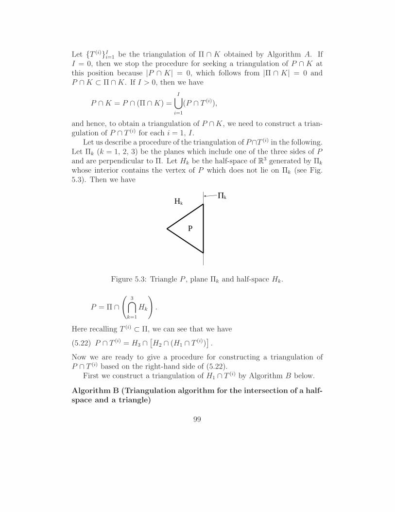
Let {T (i)}Ii=1 be the triangulation of Π ∩ K obtained by Algorithm A. If

I = 0, then we stop the procedure for seeking a triangulation of P ∩ K atthis position because |P ∩ K| = 0, which follows from |Π ∩ K| = 0 andP ∩ K ⊂ Π ∩ K. If I > 0, then we have

P ∩ K = P ∩ (Π ∩ K) =I⋃

i=1

(P ∩ T (i)),

and hence, to obtain a triangulation of P ∩K, we need to construct a trian-gulation of P ∩ T (i) for each i = 1, I.

Let us describe a procedure of the triangulation of P∩T (i) in the following.Let Πk (k = 1, 2, 3) be the planes which include one of the three sides of Pand are perpendicular to Π. Let Hk be the half-space of R3 generated by Πk

whose interior contains the vertex of P which does not lie on Πk (see Fig.5.3). Then we have

HΠ

k

P

k

Figure 5.3: Triangle P , plane Πk and half-space Hk.

P = Π ∩(

3⋂k=1

Hk

).

Here recalling T (i) ⊂ Π, we can see that we have

(5.22) P ∩ T (i) = H3 ∩[H2 ∩ (H1 ∩ T (i))

].

Now we are ready to give a procedure for constructing a triangulation ofP ∩ T (i) based on the right-hand side of (5.22).

First we construct a triangulation of H1 ∩ T (i) by Algorithm B below.

Algorithm B (Triangulation algorithm for the intersection of a half-space and a triangle)

99

Input: A half-space H and a triangle T .

Output: A triangulation {Tj}Jj=1 of H ∩ T .

Procedure: Count the number n+ of vertices of T included in the interiorof H and the number n0 of vertices of T lying on the boundary Π ofH . For each (n0, n+), the shape of H ∩ T is determined as listed inTable 5.2. Seek vertices of H ∩ T following Table 5.2, where {v+

n }n+

n=1,

{v0n}

n0

n=1 and {v−n }

3−n+−n0

n=1 represent the vertices of T contained in theinterior, the boundary and the exterior of H , respectively.

Let {Tj}Jj=1 be the triangulation of H1 ∩ T (i) obtained by Algorithm B. If

J = 0, then stop seeking a triangulation of P ∩ T (i) because |P ∩ T (i)| = 0,which follows from |H1 ∩ T (i)| = 0 and P ∩ T (i) ⊂ H1 ∩ T (i). If J > 0, thenwe have

H2 ∩ (H1 ∩ T (i)) = H2 ∩(

J⋃j=1

Tj

)=

J⋃j=1

(H2 ∩ Tj).

Hence, next constructing a triangulation of H2 ∩ Tj for each j = 1, J byAlgorithm B and combining them, we can get a triangulation of H2 ∩ (H1 ∩T (i)), which is denoted by

{T ′

j

}J ′

j=1. If J ′ = 0, then we can see that |P ∩

T (i)| = 0 in the same argument as above, and hence we stop the procedurefor constructing a triangulation of P ∩ T (i) at this position. If J ′ > 0, thenwe have

(5.23) H3 ∩ [H2 ∩ (H1 ∩ T (i))] = H3 ∩(

J ′⋃j=1

T ′j

)=

J ′⋃j=1

(H3 ∩ T ′j).

Hence, finally constructing a triangulation of H3∩T ′j for each j = 1, . . . , J ′ by

Algorithm B and combining them, we can obtain a triangulation of P ∩T (i),which can be understood from (5.22) and (5.23).

We summarize the above procedure for constructing a triangulation ofthe intersection of a tetrahedron and a triangle as Algorithm 1. To avoida complicated description, we summarize the procedure for constructing atriangulation of P ∩ T (i) appearing in the above procedure as Algorithm 2after describing Algorithm 1.

Algorithm 1

100

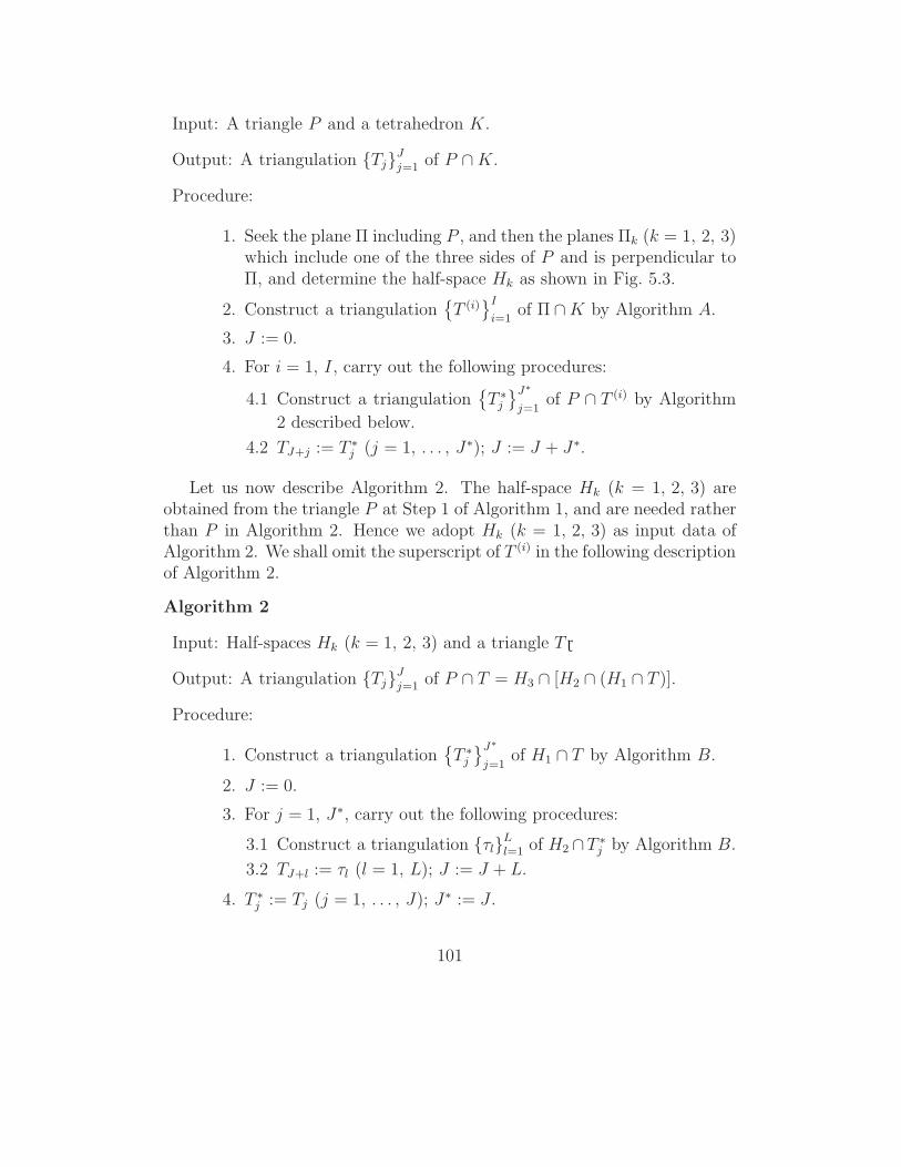
Input: A triangle P and a tetrahedron K.

Output: A triangulation {Tj}Jj=1 of P ∩ K.

Procedure:

1. Seek the plane Π including P , and then the planes Πk (k = 1, 2, 3)which include one of the three sides of P and is perpendicular toΠ, and determine the half-space Hk as shown in Fig. 5.3.

2. Construct a triangulation{T (i)}I

i=1of Π ∩ K by Algorithm A.

3. J := 0.

4. For i = 1, I, carry out the following procedures:

4.1 Construct a triangulation{T ∗

j

}J∗

j=1of P ∩ T (i) by Algorithm

2 described below.

4.2 TJ+j := T ∗j (j = 1, . . . , J∗); J := J + J∗.

Let us now describe Algorithm 2. The half-space Hk (k = 1, 2, 3) areobtained from the triangle P at Step 1 of Algorithm 1, and are needed ratherthan P in Algorithm 2. Hence we adopt Hk (k = 1, 2, 3) as input data ofAlgorithm 2. We shall omit the superscript of T (i) in the following descriptionof Algorithm 2.

Algorithm 2

Input: Half-spaces Hk (k = 1, 2, 3) and a triangle T．

Output: A triangulation {Tj}Jj=1 of P ∩ T = H3 ∩ [H2 ∩ (H1 ∩ T )].

Procedure:

1. Construct a triangulation{T ∗

j

}J∗

j=1of H1 ∩ T by Algorithm B.

2. J := 0.

3. For j = 1, J∗, carry out the following procedures:

3.1 Construct a triangulation {τl}Ll=1 of H2 ∩T ∗

j by Algorithm B.

3.2 TJ+l := τl (l = 1, L); J := J + L.

4. T ∗j := Tj (j = 1, . . . , J); J∗ := J .

101

5. J := 0.

6. For j = 1, . . . , J∗, carry out the following procedures:

6.1 Construct a triangulation {τl}Ll=1 of H3 ∩T ∗

j by Algorithm B.

6.2 TJ+l := τl (l = 1, L); J := J + L.

Remark 5.2 The number of triangles contained in a triangulation obtainedby Algorithm 2 is less than or equal to 8. This is because the number oftriangles contained in a triangulation obtained by Algorithm B is less than orequal to 2. Further, since the number of triangles contained in a triangulationobtained by Algorithm A is less than or equal to 2, we can see that the numberof triangles contained in a triangulation obtained by Algorithm 1 is less thanor equal to 16.

5.2.2 Algorithm for computing the entries of matrixBγ

Algorithm 3

Input: A tetrahedrization {Kl}Ll=1 and a triangulation {Pm}Mm=1.

Output：The (m, n)-entry bm,n of matrix Bγ (1 ≤ m ≤ M, 1 ≤ n ≤ N ).

Procedure:

1. bm,n := 0 (1 ≤ m ≤ M, 1 ≤ n ≤ N ).

2. For m = 1, . . . , M, do:

2.1 For Pm, seek planes Π and Πk (k = 1, 2, 3) by the procedureat Step 1 of Algorithm 1, and determine the half-space Hk asshown in Fig. 5.3.

2.2 For l = 1, . . . , L, do:

2.2.1 Construct a triangulation {Tj}Jj=1 of Pm ∩Kl by the pro-

cedures at Steps 2–4 of Algorithm 1.

2.2.2 For j = 1, . . . , J , do:

∗ Seek the barycentre Gj of the triangle Tj .

∗ Let nk (k = 1, . . . , 4) be the nodal numbers of verticesof Kl. Then

bm,nk:= bm,nk

+ ϕnk(Gj)|Tj| (k = 1, . . . , 4).

102

Remark 5.3 If triangular patch Pm and a face T of tetrahedral element Kl1

are coplanar, there exists the other tetrahedral element Kl2 sharing T as oneof its faces. The plane Π is computed at Step 2.1, and then for each l = l1, l2at Step 2.2, the case of N0 = 3 in Table 5.1 arises in Algorithm A whichis called in Algorithm 1 at Step 2.2.1. Then, in one case, N+ = 0, andin the other case, N+ = 1. By outputting T (= Π ∩ Kl1 = Π ∩ Kl2) onlywhen N+ = 0, we can avoid overadding its contribution to the correspondingentries of matrix Bγ.

Remark 5.4 To compute the entries of matrix A in (5.19), we must com-pute

s(ϕp, ϕq) =∞∑

n=0

n∑m=−n

−ka2 h(1)′n (ka)

h(1)n (ka)

(ϕp)mn (a)(ϕq)m

n (a) (1 ≤ p, q ≤ N )

with

(5.24) (ϕp)mn (a) =

∫ 2π

0

dφ

∫ π

0

ϕp(a, θ, φ)Y mn (θ, φ) sin θ dθ,

where a is the radius of the artificial boundary Γa. We can compute theFourier coefficients (5.24) approximately in the following way: First we ap-proximate the artificial boundary Γa by finite triangular patches. Next weapproximate the spherical harmonics Y m

n by piecewise constant functions onthe triangulation of Γa. Finally we use Algorithm 3 with an obvious modifi-cation to compute (5.24) approximately.

5.2.3 The effect of numerical error

In this subsection, we show that Algorithm 3 is numerically robust in thesense that it always carries out its task ending up with some output (cf.[122]), if we take two simple measures described below. Then we assumethat neither any tetrahedron of an input tetrahedrization nor any triangle ofan input triangulation degenerates or nearly degenerates. This assumptionis proper, since the use of any degenerate or nearly degenerate elements isnot desirable in the finite element computations. Moreover, the assumptionimplies that planes Π and Πk (k = 1, 2, 3) are normally computed at Step2.1 of Algorithm 3.

103

The first measure is taken in the procedure for computing the intersectionof plane Π and a line segment whose endpoints lie in both sides of Π inAlgorithms A and B. Let (x0, y0, z0) and (x1, y1, z1) be the coordinates ofthe endpoints of the line segment, and let ax+by+cz+d = 0 be the Cartesianequation of plane Π. Then compute the point of intersection (x, y, z) by thefollowing procedure:

1. ti := axi + byi + czi + d (i = 0, 1);

2. t :=−t0

t1 − t0;

3.

⎡⎣ xyz

⎤⎦ = t

⎡⎣ x1 − x0

y1 − y0

z1 − z0

⎤⎦+

⎡⎣ x0

y0

z0

⎤⎦ .

A remarkable point of this procedure is that we can assure t1 − t0 �= 0even in floating-point arithmetic. This reason can be understood as follows.We judge by sign of ti (i = 0, 1) which of the half-spaces generated by Πcontains (xi, yi, zi). Hence, t0 and t1 are mutually different sign floatingpoint numbers. This implies t1 − t0 �= 0. Therefore, division by zero does nottake place if we seek the point of intersection by the procedure above.

The second measure is taken in Algorithm B. Numerical errors cause adegenerate triangle to be inputted into Algorithm B (for details, see below).If a degenerate triangle is inputted, the case of n0 = 3 can occur. So we mustadd the case of n0 = 3, and in such a case, we put J = 0, that is, we makethe output triangulation void.

Let us show that if the two measures above are taken, then Algorithm 3is numerically robust.

First, we consider Algorithms A and B. We note that the main procedureof these algorithms is to compute the intersection of a plane and a line seg-ment whose endpoints lie in both sides of the plane. From the assumptionof this subsection, a normal tetrahedron and a normal plane are inputtedinto Algorithm A. Therefore, we can see that the first measure preventsAlgorithm A from failing. On the other hand, a degenerate triangle can beinputted into Algorithm B; however, in such a case, the first and secondmeasures prevent it from failing as well.

Next, we consider each step of Algorithm 3. Step 2.1 is assumed to worknormally in this subsection. For Step 2.2.1, we have only to consider Steps

104

2 and 4.1 of Algorithm 1. As described above, at Step 2 of Algorithm 1,Algorithm A normally works; however, its output triangulation can includesome degenerate triangles. In the case when some degenerate triangle areincluded, they are inputted into Algorithm 2 at Step 4.1 of Algorithm 1, andthen are inputted into Algorithm B at Step 1 of Algorithm 2. In Algorithm2, Algorithm B plays an essential role. As mentioned above, Algorithm Bdoes not fail even if a degenerate triangle is inputted into it. Thus, wecan see that any failures do not occur at Step 4.1 of Algorithm 1. Thisimplies that any failures do not occur at Step 2.2.1 of Algorithm 3. Also,a triangulation outputted at Step 2.2.1 of Algorithm 3 can include somedegenerate triangles; however, even in such a case, any failures do not occurat Step 2.2.2 of Algorithm 3 because we only compute the barycentres andthe measures of triangles there.

From the above, we can prove that if the two measures above are taken,Algorithm 3 does not fail.

Remark 5.5 Although we follow the right-hand side of (5.22) to constructa triangulation of P ∩ T in Algorithm 2, we can also triangulate P ∩ T byrepresenting T as the intersection of three half-spaces and Π, that is, by using

T = Π ∩(

3⋂k=1

H ′k

)

and

P ∩ T = H ′3 ∩ [H ′

2 ∩ (H ′1 ∩ P )] .

However, since T can be a degenerate triangle, we then can not computesome of the planes Π′

k := ∂H ′k. This fact can be the cause of the failure of

the algorithm.

5.3 Simplification of the algorithm

We have seen from the consideration of Section 5.2.3 that the two measuresprevent Algorithm 3 from failing even if some degenerate triangles occur in it.So, in this section, we simplify Algorithms A and B by allowing their outputtriangulations containing some degenerate triangles even if the arithmetic isexact.

105

Although Algorithm A determine its procedure for each case of (N0, N+),we simplify it by using only N+ to determine the procedure, that is, foreach N+ = 0, 1, . . . , 4, a simplified algorithm executes the procedure for thecase of (N0, N+) = (0, N+) of Algorithm A. Note that in the simplifiedalgorithm, {v+

n }N+

n=1 and {v−n }

4−N+

n=1 in Table 5.1 denote the vertices of Kthat are contained in the interior of H and the vertices of K that are notcontained in the interior of H , respectively. This simplified algorithm will becalled Algorithm A∗ in the sequel.

We can analogously give a simplified algorithm of Algorithm B, AlgorithmB∗. For each n+ = 0, 1, . . . , 3, Algorithm B∗ executes the procedure for thecase of (n0, n+) = (0, n+) of Algorithm B. In the Algorithm B∗, {v+

n }n+

n=1

and {v−n }

3−n+

n=1 in Table 5.2 represent the vertices of T that are contained inthe interior of H and the vertices of T that are not contained in the interiorof H , respectively.

When we employ Algorithms A∗ and B∗ instead of Algorithms A andB in Algorithm 3, we shall call such an algorithm Algorithm 3∗. A similarargument to Section 5.2.3 shows that the first measure prevents Algorithm3∗ form failing.

In the sequel of this section, we discuss under the assumption that thearithmetic is executed exactly.

We consider the difference between Algorithms A and A∗ for an input{K, Π} with tetrahedron K and plane Π.

If the output triangulation of Algorithm A is {Tj}Jj=1, then the output

triangulation of Algorithm A∗ are represented by {Tj}Jj=1 ∪ {T ′

j}J ′j=1, where

T ′j are degenerate triangles and J ′ satisfies 0 ≤ J ′ ≤ 2.

If a vertex of K lies on Π and if it becomes a vertex of an output triangle,then, in Algorithm A, it is directly employed; but, on the other hand, inAlgorithm A∗, it is recomputed by executing the procedure for computing thepoint of intersection. Hence, the number of seeking the point of intersectionin Algorithm A∗ is more than that in Algorithm A.

These facts hold between Algorithms B and B∗ as well.From the argument above, we can conclude that the number of seeking

the point of intersection and the number of triangles generated in the processof Algorithm 3∗ are more than those in the process of Algorithm 3.

106

5.4 Numerical experiments

In this section, we compare Algorithm 3 with Algorithm 3∗ through numericalexperiments.

In our numerical experiments, as the fictitious domain Ω, we choose acube with the length 4 of an edge: Ω = (−2, 2)3, and as the obstacle O, wetake the following five kinds of obstacles:

1. Cube: O = (−1, 1)3.

2. Regular icosahedron: it is circumscribed by the unit sphere centered onthe origin, and has the regular triangle with vertices: (0, 0, 1), (s, 0, c)and (s cos 2π

5, s sin 2π

5, c) as one of its faces, where c = cos(2π/5)/[1 −

cos(2π/5)] and s =√

1 − c2.

3. Sphere: O = {x ∈ R3 | |x| < 1}.

4. Right circular cylinder: O = {x = (x1, x2, x3) ∈ R3 | x2

1 + x23 <

(1/2)2, −1 < x2 < 1}.

5. Regular octahedron: it is circumscribed by the sphere of radius a/√

2centered on the origin, and has the regular triangle with vertices:(a/2, −a/2, 0), (a/2, a/2, 0) and (0, 0, a/

√2) as one of its faces, where

a = 9/8.

In this numerical experiment, we consider two kinds of tetrahedrizationsof domain Ω and two kinds of triangulations of boundary γ of each obstacleO, and call the coarser one of these divisions the first divisions, and the otherthe second divisions.

The ith (i = 1, 2) division of domain Ω is generated as follows: first

Ω is subdivided into (128 × 2(i−1))3 congruent cubes and next each cube issubdivided into six tetrahedrons (see Fig. 5.4). We do not describe howto triangulate boundary γ of each obstacle O in detail; however, we shalldescribe the triangulations of γ in Remark 5.6 when O is the cube, becausesuch triangulations are taken to be special ones which are associated with thetetrahedrizations of Ω. Now let h be the mesh length of Ω in the directionof each coordinate axis, and let ηmin be the minimum length of the minimumside of each triangle belonging to the triangulation of γ. In each divisions,the following relation is satisfied:

ηmin ≥ 2h,

107

which is a three dimensional analogue to the result of Girault-Glowinski [44]for the two dimensional problem. In [44], they state that the mesh size of

γ should be taken slightly larger than that of Ω in order to get appropriatenumerical solutions.

x1x2

x3

Figure 5.4: Tetrahedrization of Ω (also triangulation of γ when O is a cube).

Remark 5.6 When O is the cube, in the ith (i = 1, 2) division of γ, everyface of γ is subdivided into [64 × 2(i−1)]2 right-angled isosceles triangle asdepicted in Fig. 5.4. Further, in both the first and the second divisions, everytriangle P of the triangulation becomes the union of faces of four tetrahedronsof the tetrahedrization as shown in Fig. 5.5.

P

Figure 5.5: Left: An arbitrary triangular patch P ; Right: P becomes theunion of faces of four tetrahedral elements.

In the numerical experiments, we examine the execution time T [s] ofAlgorithms 3 and 3∗, the number L of seeking the point of intersection inAlgorithms 3 and 3∗, and the number Nz of entries of matrix B that are

108

judged to be non-zero. Further, we examine the quantities that will beexplained in the following. For each triangular patch Pm (m = 1, 2, . . . , M),

let {T (m)j }Jm

j=1 be the triangulation obtained at Step 2.2 of Algorithm 3 (or 3∗).Note that the triangulation may include some degenerate triangles. Then wedefine

J =

M∑m=1

Jm.

Since J equals the number of computing the barycentre or the measure of thetriangles at Step 2.2.2, we can consider that J is the quantity that stronglyinfluences the execution time T . Furthermore, as an error, we compute

e =

M∑m=1

∣∣∣∣∣|Pm| −Jm∑j=1

|T (m)j |∣∣∣∣∣ ,

where |Pm| denotes the measure of Pm.In the computations, we used a PC whose CPU is Xeon 3.4GHz and main

memory is 8GB. As an complier, we employed Intel Fortran Compiler ver.8.1. We computed with double precision arithmetic.

We summarize the numerical results in Tables 5.3 and 5.4, where for eachO, the results for the first division and for the second division are listed in theupper two rows and the lower two rows, respectively, and in each of those tworows the results for Algorithm 3 and for Algorithm 3∗ are listed in the upperrow and the lower row, respectively. Further the ratios of J∗/J and L∗/Lare also listed in Table 5.4, where J∗ are L∗ denotes J and L correspondingto Algorithm 3∗, respectively.

Table 5.3 shows that there are a few cases where Nz of Algorithm 3∗ islarger than that of Algorithm 3, and that the errors e of these algorithms arenot different from each other.

Table 5.4 illustrates that in the two cases when O is the cube and thecylinder, Algorithm 3∗ takes more time than Algorithm 3. Especially, in thecase of the cube, the execution time T of Algorithm 3∗ is more than twicethat of Algorithm 3. In the other cases, Algorithm 3∗ takes less time thanAlgorithm 3. We can observe that the execution time tends to depend onthe values of J∗/J and L∗/L. These values for the cube is the largest in thevalues listed in Table 5.4. The second largest values are for the cylinder.

We can see that if the values of J∗/J and L∗/L is some larger, thatis, if the number of triangles generated in Algorithm 3∗ and the number of

109

computing the point of intersection in Algorithm 3∗ are some larger thanthose of Algorithm 3, the execution time of Algorithm 3∗ becomes longerthan that of Algorithm 3. One reason why the values of J∗/J and L∗/Lincrease seems to be that faces of γ are contained in division faces of thetetrahedrization of Ω. Because such a situation occurs only in the two caseswhen O is the cube and the cylinder. Indeed, as described in Remark 5.6,when O is the cube, every face of γ is contained in a division face of Ω.Also, when O is the cylinder, the two bases of the cylinder are contained indivision faces of Ω. Moreover, when O is the cube, every triangular patchbecomes the union of faces of four tetrahedral elements as depicted in Fig.5.5. We can consider that this fact also causes the values of J∗/J and L∗/Lto increase.

Although the case when O is the cube is an disadvantage example forAlgorithm 3∗, we note that such an example is not meaningful in practicalcomputations.

One reason why there are cases where the execution time of Algorithm3∗ is shorter than that of Algorithm 3 is that the number of selectors of thecase construct of the Fortran program for Algorithm 3∗ is less than that ofAlgorithm 3.

Although the execution times for Algorithms 3 and 3∗ are almost thesame except for the case of the cube, the execution time of Algorithm 3∗ isslightly shorter than that of Algorithm 3 in the cases except the two caseswhen O is the cube and the cylinder. Further, the program for Algorithm3∗ is slightly simpler than that for Algorithm 3. Therefore, we can concludethat the simplified algorithm described in Section 5.3 is effective in practicalcomputations.

5.5 Conclusions

We have presented a fictitious domain formulation for problem (5.2) to nu-merically solve the 3D exterior Helmholtz problem. We have shown thatthe problem on the fictitious domain method has a unique solution whoserestriction to the original domain Ωa coincide with the solution of (5.2).

Further, we have presented an algorithm for computing the entries of theconstraint matrix arising in the resulting system of linear equations. Wehave shown that degenerate triangles generated due to numerical errors donot cause the algorithm to fail. On the basis of this fact, we have designed

110

one simplified algorithm, and have shown its effectiveness through numericalexperiments.

Practical computations in this fictitious domain formulation and the math-ematical analysis for the associated discrete problem (5.18) are yet to bedone.

111

Table 5.1: Shape of Π ∩ K and procedure to output a triangulation {Tj}Jj=1

of Π ∩ K for each (N0, N+).N0 N+ Π ∩ K J Vertices of Π ∩ K we

need to computeVertices of Tj (j =1, J)

0 0 Empty 0 – –1 A triangle 1 The point of intersec-

tion pk of the plane Πand the edge joining v+

1

and v−k (k = 1, 2, 3)

T1 := {p1, p2, p3}

2 A quadrangle 2 The point of intersec-tion pkl of the plane Πand the edge joining v+

k

and v−l (k, l = 1, 2)

T1 := {p11, p22, p12},T2 := {p11, p22, p21}

3 A triangle 1 The point of intersec-tion pk of the plane Πand the edge joining v+

k

and v−1 (k = 1, 2, 3)

T1 := {p1, p2, p3}

4 Empty 0 – –1 0 A point 0 – –


1

and v−k (k = 1, 2)

T1 := {v01, p1, p2}


k

and v−1 (k = 1, 2)

T1 := {v01, p1, p2}

3 A point 0 – –2 0 A line segment 0 – –

1 A triangle 1 The point of intersec-tion p1 of the plane Πand the edge joining v+

1

and v−1

T1 := {v01, v0

2 , p1}

2 A line segment 0 – –3 0 A triangle 1 – T1 := {v0

1, v02 , v0

3}1 A triangle 0 – –

112

Table 5.2: Shape of H ∩ T and procedure to output a triangulation {Tj}Jj=1

of H ∩ T for each (n0, n+).n0 n+ H ∩ T J Vertices of H ∩ T we

need to computeVertices of Tj (j =1, J)

0 0 Empty 0 – –1 A triangle 1 The point of intersec-

tion pk of the plane Πand the side joining v+

1

and v−k (k = 1, 2)

T1 := {v+1 , p1, p2}

2 A quadrangle 2 The point of intersec-tion pk of the plane Πand the side joining v+

k

and v−1 (k = 1, 2)

T1 := {v+1 , v+

2 , p1},T2 := {v+

2 , p1, p2}

3 A triangle 1 – T1 := {v+1 , v+

2 , v+3 }

1 0 A point 0 – –1 A triangle 1 The point of intersec-

tion p1 of the plane Πand the side joining v+

1

and v−1

T1 := {v+1 , v0

1, p1}

2 A triangle 1 – T1 := {v+1 , v+

2 , v01}

2 0 A line segment 0 – –1 A triangle 1 – T1 := {v+

1 , v01, v0

2}

113

Table 5.3: Computational results I.O h ηmin M Nz ecube 3.125E-2 6.25E-2 12,288 110,592 0.00

110,592 0.001.5625E-2 3.125E-2 49,152 442,368 0.00

442,368 0.00icosahedron 3.125E-2 6.57E-2 5,120 101,580 8.16E-14

101,580 8.16E-141.5625E-2 3.29E-2 20,480 405,983 3.12E-13

405,983 3.12E-13sphere 3.125E-2 6.92E-2 5,120 118,260 9.61E-14

118,260 9.61E-141.5625E-2 3.46E-2 20,480 473,290 3.72E-13

473,291 3.72E-13cylinder 3.125E-2 7.17E-2 1,610 52,613 2.17E-14

52,689 2.17E-141.5625E-2 3.53E-2 6,526 212,370 7.01E-14

212,448 7.01E-14octahedron 3.125E-2 7.03E-2 2,048 41,189 9.96E-15

41,189 9.96E-151.5625E-2 3.52E-2 8,192 166,693 3.19E-14

166,693 3.19E-14

114

Table 5.4: Computational results II.O J J∗/J L L∗/L Tcube 49,152 4.5 0 ∞ 0.400

221,184 4,845,568 0.835196,608 4.5 0 ∞ 1.68884,736 19,382,272 3.42

icosahedron 261,589 1.0022 2,167,138 1.0012 0.538262,155 2,169,844 0.534

1,045,836 1.0006 8,615,212 1.0003 2.161,046,432 8,618,162 2.14

sphere 312,751 1.0009 2,510,750 1.0008 0.634313,029 2,512,824 0.633

1,254,046 1.0003 10,048,568 1.0003 2.621,254,416 10,051,212 2.60

cylinder 147,627 1.0378 1,057,801 1.0544 0.303153,207 1,115,366 0.308610,410 1.0158 4,399,377 1.0211 1.25620,025 4,492,180 1.27

octahedron 108,830 1.0099 897,990 1.0209 0.239109,902 916,784 0.236443,684 1.0035 364,3517 1.0059 0.980445,234 366,5166 0.976

115

Appendix A

Some Properties of the HankelFunctions

Lemma A.1 For all x > 0 and for all ν ∈ R, we have

Re

{H

(1)′ν (x)

H(1)ν (x)

}< 0.

Proof. Since H(1)ν (x) = Jν(x)+ iNν(x), where Jν and Nν are the cylindrical

Bessel function and the cylindrical Neumann function of order ν, respectively,we have

(A.1) Re

{H

(1)′ν (x)

H(1)ν (x)

}=

Jν(x)J ′ν(x) + Nν(x)N ′

ν(x)

J2ν (x) + N2

ν (x).

According to Watson [130, p. 444], we have Nicholson’s formula:

(A.2) J2ν (x) + N2

ν (x) =8

π2

∫ ∞

0

K0(2x sinh t) cosh(2νt) dt,

where K0 is the modified Bessel function of the second kind of order zero.Differentiating (A.2) with x, we obtain

(A.3) Jν(x)J ′ν(x) + Nν(x)N ′

ν(x) =8

π2

∫ ∞

0

K ′0(2x sinh t) sinh t cosh(2νt) dt.

Now we note that we have the following formula:

(A.4) K0(ξ) =

∫ ∞

0

e−ξ cosh t dt for all ξ > 0

116

(see Abramowitz and Stegun [1], Watson [130]). Differentiating (A.4) withξ, we can get

(A.5) K ′0(ξ) = −

∫ ∞

0

e−ξ cosh t cosh t dt < 0 for all ξ > 0.

Combining (A.1), (A.3) and (A.5) completes the proof of Lemma A.1.

Lemma A.2 For all x > 0 and for all ν, ν ′ ∈ R satisfying |ν| > |ν ′|, we have

(A.6) 0 < Im

{H

(1)′ν (x)

H(1)ν (x)

}< Im

{H

(1)′ν′ (x)

H(1)ν′ (x)

}.

Proof. We have the following formulas:

H(1)′ν (x) = H

(1)ν−1(x) − ν

xH(1)

ν (x),

Jν−1(x)Nν(x) − Jν(x)Nν−1(x) = − 2

πx(see [1]).

Using these formulas, we can get

(A.7) Im

{H

(1)′ν (x)

H(1)ν (x)

}=

2

πx

1

J2ν (x) + N2

ν (x)> 0.

Now it follows from (A.4) that K0(2x sinh t), being in the integral on theright-hand side of (A.2), is a positive function of t on (0, ∞). Thus, we caneasily see from (A.2) that for all ν, ν ′ ∈ R satisfying |ν| > |ν ′|,

(A.8) J2ν (x) + N2

ν (x) > J2ν′(x) + N2

ν′(x).

From (A.7) and (A.8), we can get (A.6).

Lemma A.3 Im

{H

(1)′0 (x)

H(1)0 (x)

}is a decreasing function in (0, ∞). Further

(A.9) Im

{H

(1)′0 (x)

H(1)0 (x)

}−→ 1 as x −→ +∞

and

(A.10) Im

{H

(1)′0 (x)

H(1)0 (x)

}−→ +∞ as x −→ +0.

117

Proof. According to [130], x(J20 (x) + N2

0 (x)) is an increasing function in(0, ∞). This implies that

(A.11) Im

{H

(1)′0 (x)

H(1)0 (x)

}=

2

πx

1

J20 (x) + N2

0 (x)

is a decreasing function in (0, ∞).We have

(A.12) H(1)0 (x) ∼

√2

πxei(x−π/4) as x −→ +∞ (see [1]).

Further we can see from (A.11) that

(A.13) Im

{H

(1)′0 (x)

H(1)0 (x)

}=

∣∣∣√ 2πx

ei(x−π/4)∣∣∣2∣∣∣H(1)

0 (x)∣∣∣2 .

From (A.12) and (A.13), we can get (A.9).Since J0(0) = 1 and N0(x) ∼ (2/π) logx as x −→ +0 (see [1]), we have

x{J20 (x)+N2

0 (x)} = xJ20 (x)+x

(2

πlog x

)2 [N0(x)2π

log x

]2−→ 0 as x −→ +0,

and hence (A.11) yields (A.10).

Lemma A.4 For all x > 0 and for all n ∈ N ∪ {0}, we have

Re

{h

(1)′n (x)

h(1)n (x)

}< 0.

Proof. Since

h(1)n (x) =

√π

2xH

(1)n+1/2(x),

we have

(A.14)h

(1)′n (x)

h(1)n (x)

= − 1

2x+

H(1)′n+1/2(x)

H(1)n+1/2(x)

.

118

Thus, we can see form Lemma A.1 that

Re

{h

(1)′n (x)

h(1)n (x)

}= − 1

2x+ Re

{H

(1)′n+1/2(x)

H(1)n+1/2(x)

}< 0.

Lemma A.5 For all x > 0 and for all n ∈ N, we have

0 < Im

{h

(1)′n (x)

h(1)n (x)

}< Im

{h

(1)′0 (x)

h(1)0 (x)

}≡ 1.

Proof. From (A.14), we can get

Im

{h

(1)′n (x)

h(1)n (x)

}= Im

{H

(1)′n+1/2(x)

H(1)n+1/2(x)

}.

Thus, by Lemma A.2, we have

0 < Im

{h

(1)′n (x)

h(1)n (x)

}< Im

{h

(1)′0 (x)

h(1)0 (x)

}for all n ∈ N.

Since h(1)0 (x) = −ieix/x, we can see that

Im

{h

(1)′0 (x)

h(1)0 (x)

}≡ 1.

Lemma A.6 For each x > 0, there exists a positive constant C such that

(A.15)

∣∣∣∣∣ 1

1 + |n|H

(1)′n (x)

H(1)n (x)

∣∣∣∣∣ ≤ C for all n ∈ Z,

(A.16)

∣∣∣∣∣ 1

1 + n

h(1)′n (x)

h(1)n (x)

∣∣∣∣∣ ≤ C for all n ∈ N ∪ {0},

where C depends on x, but is independent of n.

119

Proof. For proofs of (A.15) and (A.16), see [105] and [81], respectively.

Lemma A.7 For any r1 > r2 > 0,∣∣∣H(1)

ν (r1)/H(1)ν (r2)

∣∣∣ is a decreasing func-

tion of ν on [0, ∞), and further∣∣∣h(1)

n (r1)/h(1)n (r2)

∣∣∣ is a decreasing sequence

of n ∈ N ∪ {0}.

Proof. We first prove the former assertion. We write

F (ν; r) =∣∣H(1)

ν (r)∣∣2.

From Nicholson’s formula:

(A.17) F (ν; r) =8

π2

∫ ∞

0

K0(2r sinh t) cosh(2νt) dt (ν ∈ R, r > 0),

we see that, for each r > 0, F (·; r) ∈ C∞(R) and F (·; r) > 0. Thus, it issufficient to show that

d

dν

(F (ν; r1)

F (ν; r2)

)< 0

for all ν ∈ (0, ∞). This inequality holds if and only if

(A.18)dF

dν(ν; r1)F (ν; r2) − F (ν; r1)

dF

dν(ν; r2) < 0.

Hence, let us prove (A.18) in the following. Differentiating (A.17) with νleads to

(A.19)dF

dν(ν; r) =

16

π2

∫ ∞

0

K0(2r sinh t)t sinh(2νt) dt.

From (A.17) and (A.19), we have

dF

dν(ν; r1)F (ν; r2) − F (ν; r1)

dF

dν(ν; r2)(A.20)

=128

π4

∫ ∞

0

∫ ∞

0

[K0(2r1 sinh t1)K0(2r2 sinh t2)t1 sinh(2νt1) cosh(2νt2)

−K0(2r2 sinh t1)K0(2r1 sinh t2)t1 sinh(2νt1) cosh(2νt2)] dt1dt2

=128

π4

∫ ∞

0

dt1∫ t1

0

[K0(2r1 sinh t1)K0(2r2 sinh t2) − K0(2r1 sinh t2)K0(2r2 sinh t1)]

× [t1 sinh(2νt1) cosh(2νt2) − t2 sinh(2νt2) cosh(2νt1)] dt2.

120

Here, using Macdnold’s formula (see [130, p. 439]):

K0(X)K0(x) =1

2

∫ ∞

0

exp

[− t

2− X2 + x2

2t

]K0

(Xx

t

)dt

t(X, x > 0)

and the fact that

(r21 sinh2 t1 + r2

2 sinh2 t2) − (r21 sinh2 t2 + r2

2 sinh2 t1)

= (r21 − r2

2)(sinh2 t1 − sinh2 t2) > 0

for t1 > t2 > 0, we can conclude that

(A.21) K0(2r1 sinh t1)K0(2r2 sinh t2) − K0(2r1 sinh t2)K0(2r2 sinh t1) < 0

for t1 > t2 > 0. Further, we have

t1 sinh(2νt1) cosh(2νt2) − t2 sinh(2νt2) cosh(2νt1)(A.22)

=1

2{(t1 − t2) sinh[2ν(t1 + t2)] + (t1 + t2) sinh[2ν(t1 − t2)]} > 0

for t1 > t2 > 0. From (A.20)–(A.22), we deduce (A.18).We next prove the latter assertion. Since

h(1)n (r) =

√π

2rH

(1)n+1/2(r),

we have∣∣∣∣∣h(1)n (r1)

h(1)n (r2)

∣∣∣∣∣ =√

r2

r1

∣∣∣∣∣H(1)n+1/2(r1)

H(1)n+1/2(r2)

∣∣∣∣∣ .Hence, it follows from the above result that

∣∣∣h(1)n (r1)/h

(1)n (r2)

∣∣∣ is a decreasing

sequence of n ∈ N ∪ {0}.

121

Appendix B

Well-posedness of the WaveEquation with a DtN BoundaryCondition

B.1 Proof of Theorem 4.1

We first state two lemmas concerning properties of σn.

Lemma B.1 We have

σn − |n|a

∼ k2a

2|n| as n −→ ±∞.

Proof. See [105].

Lemma B.2 For all n ∈ Z, Re(σn) > 0.

Proof. See [93].

Define

Bϕ =∞∑

n=−∞Re(σn)ϕnYn for every ϕ ∈ H1/2(Γa).

It follows from Lemma B.1 that B is a bounded linear operator form H1/2(Γa)into H−1/2(Γa). Further we see from Lemma B.2 that

〈Bϕ, ϕ〉 ≥ 0 for all ϕ ∈ H1/2(Γa).

122

The space E becomes a Hilbert space equipped with the inner product:

(u, v)E =

∫Ωa

∇u0 · ∇v0 dx +

∫Ωa

u1v1 dx + 〈Bu0, v0〉

for u = {u0, u1}, v = {v0, v1} ∈ E; the associated norm is denoted by ‖ · ‖E.In order to prove Theorem 4.1, it is sufficient from Hille-Yosida’s theorem

[136] to prove three propositions described below.

Proposition B.1 D(A) is dense in E.

Proposition B.2 There exists a positive constant C such that

(B.1) Re(Au, u)E ≤ C‖u‖2E for all u ∈ D(A).

Proposition B.3 For every λ ≥ 0, there exists (λ − A)−1 as a boundedlinear operator on E.

Propositions B.1–B.3 will be proved in Subsections B.1.1–B.1.3, respec-tively.

B.1.1 Proof of Proposition B.1

To prove Proposition B.1, we use the following lemma, whose proof is de-scribed in [82].

Lemma B.3 For all g ∈ C∞(Γa) and for all ε > 0, there exists a u ∈C∞

0 (Ωa ∪ Γa) such that

u = 0 on Γa,∂u

∂n= g on Γa,

and ‖u‖H1(Ωa) ≤ ε, where

C∞0 (Ωa∪Γa) = {ϕ ∈ C∞(Ωa) | There exists a ϕ ∈ C∞

0 (Ω) such that ϕ = ϕ|Ωa} .

Proof of Proposition B.1. Let {v0, v1} be an arbitrary element of E.Since [C∞

0 (Ωa ∪ Γa)]2 is dense in E, there exist {v0j , v1j} ∈ [C∞

0 (Ωa ∪ Γa)]2

(j = 1, 2, . . .) such that

(B.2) {v0j , v1j} −→ {v0, v1} in E as j −→ ∞.

123

Define

(B.3) gj =∂v0j

∂n+ v1j + Sv0j + ikv0j on Γa.

Since gj ∈ C∞(Γa), we can see from Lemma B.3 that for each j ∈ N, thereexists a wj ∈ C∞

0 (Ωa ∪ Γa) such that

(B.4) wj = 0 on Γa,∂wj

∂n= gj on Γa,

and

(B.5) ‖wj‖H1(Ωa) ≤1

j.

It follows from (B.3) and (B.4) that {v0j − wj, v1j} ∈ D(A). Furthermore,we deduce from (B.2) and (B.5) that

{v0j − wj, v1j} −→ {v0, v1} in E as j −→ ∞.


Proof of Proposition B.2. For every u = {u0, u1} ∈ D(A), by the Greenformula, we can get

(B.6) Re(Au, u)E = −‖u1‖2L2(Γa) − Re 〈(S − B)u0, u1〉 + k Im 〈u0, u1〉 .

Set ϕ = u0|Γa and ψ = u1|Γa . Then we have

(B.7) −Re 〈(S − B)u0, u1〉 + k Im 〈u0, u1〉 =∞∑

n=−∞{k + Im(σn)} Im

(ϕnψn

).

Lemma B.1 implies that there exists a positive constant C0 such that

(B.8) |k + Im(σn)| ≤ C0 for all n ∈ Z.

Combining (B.6)–(B.8) leads to

Re(Au, u)E ≤ C20

4‖u0‖2

L2(Γa).

Thus, by the trace theorem and the Poincare inequality, we can get (B.1).

124


Suppose that u ∈ D(A) satisfies (λ−A)u = f with λ ∈ R and f ∈ E. Thenwe have

(B.9)

⎧⎪⎪⎨⎪⎪⎩−Δu0 + λ2u0 = f1 + λf0 in Ωa,

u0 = 0 on γ,

∂u0

∂n= −Su0 − iku0 − λu0 + f0 on Γa,

and

(B.10) u1 = λu0 − f0.

Hence, to prove Proposition B.3, we consider the following problem:

(B.11)

⎧⎪⎪⎨⎪⎪⎩−Δu + λ2u = f in Ωa,

u = 0 on γ,

∂u

∂n= −Su − iku − λu + g on Γa,

and prove the following proposition.

Proposition B.4 For each λ ≥ 0, for every f ∈ L2(Ωa), and for everyg ∈ H1/2(Γa), problem (B.11) has a unique solution which belongs to H2(Ωa).

We shall prove Proposition B.4 after describing the proof of PropositionB.3.

Proof of Proposition B.3. Let λ be an arbitrary non-negative number.We first show that (λ−A) is one-to-one. Suppose that u = {u0, u1} ∈ D(A)satisfies (λ − A)u = 0, then u0 satisfies (B.11) with f = 0 and g = 0, andhence it follows from Proposition B.4 that u0 = 0. Thereby (B.10) leads tou1 = 0.

We next show that (λ − A) is onto. We can see from Proposition B.4that for every f = {f0, f1} ∈ E, there exists a u0 ∈ H2(Ωa) such that u0

satisfies (B.9). Set u1 = λu0 − f0 ∈ V . Then we can immediately see thatu = {u0, u1} ∈ D(A) and (λ −A)u = f .

Let us now prove Proposition B.4.

125

We consider the following problem:

(B.12)

⎧⎪⎪⎨⎪⎪⎩−Δu = f in Ωa,

u = 0 on γ,

∂u

∂n+ T u = g on Γa,

where T is the operator defined by

T ϕ =∞∑

n=−∞

|n|a

ϕnYn.

Note that T is the DtN operator associated with the exterior Laplace problemwhere the solution is required to be bounded at infinity. It is easily seen thatT is a bounded linear operator form H1/2(Γa) into H−1/2(Γa) and satisfies

(B.13) 〈T ϕ, ϕ〉 ≥ 0 for all ϕ ∈ H1/2(Γa).

Lemma B.4 For all f ∈ L2(Ωa) and for all g ∈ H1/2(Γa), problem (B.12)has a unique solution belonging to H2(Ωa), and further we have the followinga priori estimate:

(B.14) ‖u‖H2(Ωa) ≤ C{‖f‖L2(Ωa) + ‖g‖H1/2(Γa)

},

where C is a positive constant independent of f and g.

Proof. We present only an outline of the proof. (A complete proof is de-scribed in [88].) Using the trace theorem, we can see that it suffices to provethe assertion only in the case when g = 0. It follows from Lax-Milgram’slemma that a weak formulation of problem (B.12) with g = 0 has a uniquesolution. A harmonic extension of the solution to Ω can be a unique solu-tion of the exterior Laplace problem on Ω imposing the boundedness of thesolution at infinity. (For the existence and uniqueness of the solution to theexterior Laplace problem, we refer the reader to [2].) We conclude from theusual regularity argument that such a harmonic extension belongs to H2

loc(Ω).Applying the closed graph theorem to the operator G : L2(Ωa) −→ H2(Ωa)defined by Gf = u, where u is the solution of problem (B.12) with g = 0,we obtain (B.14) with g = 0.

126

For any ε ≥ 0, we consider the following problem:

(Pε)

⎧⎪⎪⎨⎪⎪⎩Lεu := −Δu + ελ2u = f in Ωa,

u = 0 on γ,

Kεu :=∂u

∂n+ T u + εRu = g on Γa,

where R = S − T + ik + λ.

Lemma B.5 Let λ ≥ 0 and 0 ≤ ε ≤ 1. Let f ∈ L2(Ωa) and g ∈ H1/2(Γa).Assume that u ∈ H2(Ωa) satisfies (Pε). Then there exists a positive constantC such that

(B.15) ‖u‖H1(Ωa) ≤ C{‖f‖L2(Ωa) + ‖g‖L2(Γa)

},

where C is independent of λ, ε, f , g, and u.

Proof. By the Green formula, we can get∫Ωa

|∇u|2 dx + ελ2

∫Ωa

|u|2 dx + (1 − ε) 〈T u, u〉 + ε{Re 〈Su, u〉 + λ‖u‖2L2(Γa)}

= Re

∫Ωa

fu dx + Re 〈g, u〉 .

Lemma B.2 yields

(B.16) Re 〈Su, u〉 ≥ 0.

Thus it follows from (B.13), (B.16), and the conditions of ε and λ that∫Ωa

|∇u|2 dx ≤ Re

∫Ωa

fu dx + Re 〈g, u〉 .

Hence we can conclude from the Poincare inequality and the trace theoremthat (B.15) holds.

Lemma B.6 For every λ ≥ 0, there exists an α > 0 such that if, for an ε1 ∈[0, 1], problem (Pε1) has a solution belonging to H2(Ωa) for every f ∈ L2(Ωa)and for every g ∈ H1/2(Γa), then, for each ε satisfying |ε− ε1| < α, problem(Pε) has a solution belonging to H2(Ωa) for every f ∈ L2(Ωa) and for everyg ∈ H1/2(Γa).

127

Proof. For every f ∈ L2(Ωa) and for every g ∈ H1/2(Γa), let u(0) be asolution of problem (Pε1), which belongs to H2(Ωa). For p = 0, 1, 2, . . ., letu(p+1) ∈ H2(Ωa) be a solution of the following problem:⎧⎪⎨⎪⎩

Lε1u(p+1) = (ε1 − ε)λ2u(p) in Ωa,

u(p+1) = 0 on γ,

Kε1u(p+1) = (ε1 − ε)Ru(p) on Γa.

Then, by Lemma B.5, we have, for every p ∈ N ∪ {0},

(B.17) ‖u(p+1)‖H1(Ωa) ≤ C1

{|ε1 − ε|λ2‖u(p)‖L2(Ωa) + |ε1 − ε|‖Ru(p)‖L2(Γa)

},

where C1 is a positive constant independent of λ, ε, ε1, u(p), and u(p+1).Lemma B.1 implies that R is a bounded linear operator on L2(Γa). Hence,it follows from (B.17) and the trace theorem that there exists a positiveconstant C2 such that

‖u(p+1)‖H1(Ωa) ≤ C2|ε1 − ε|‖u(p)‖H1(Ωa),

where C2 is independent of ε, ε1, u(p), and u(p+1). This yields

(B.18) ‖u(p+1)‖H1(Ωa) ≤ (C2|ε1 − ε|)p+1‖u(0)‖H1(Ωa).

Set uq =∑q

p=0 u(p). Then we can see from (B.18) that if C2|ε1 − ε| < 1, then{uq}∞q=1 is a Cauchy sequence in V . Furthermore we have, for every q ∈ N,⎧⎨⎩

Lε1uq = (ε1 − ε)λ2uq−1 + f in Ωa,uq = 0 on γ,

Kε1uq = (ε1 − ε)Ruq−1 + g on Γa,

and hence, for any q > q′, uq − uq′ becomes the solution of problem (B.12)with

f = −ε1λ2(uq − uq′) + (ε1 − ε)λ2(uq−1 − uq′−1) =: fqq′,

g = −ε1R(uq − uq′) + (ε1 − ε)R(uq−1 − uq′−1) =: gqq′.

Hence, from (B.14), we have, for any q > q′,

(B.19) ‖uq − uq′‖H2(Ωa) ≤ C{‖fqq′‖L2(Ωa) + ‖gqq′‖H1/2(Γa)

}.

128

Since R is also a bounded linear operator on H1/2(Γa), (B.19) and the tracetheorem lead to

‖uq − uq′‖H2(Ωa) ≤ C{‖uq − uq′‖H1(Ωa) + ‖uq−1 − uq′−1‖H1(Ωa)

}.

This implies that {uq}∞q=1 is a Cauchy sequence in H2(Ωa) since {uq}∞q=1 is aCauchy sequence in V . Then its limit u ∈ H2(Ωa) is a solution of problem(Pε). We can see from the argument above that if we take α = 1/C2, thenthe assertion of Lemma B.6 holds.

Proof of Proposition B.4. Since, by Lemma B.4, problem (Pε) with ε = 0,i.e., problem (B.12) has a solution belonging to H2(Ωa), Lemma B.6 impliesthat problem (Pε) with ε = 1, i.e., problem (B.11) has a solution belongingto H2(Ωa). The uniqueness of the solution to problem (B.11) follows from(B.15).

129

Bibliography

[1] M. Abramowitz, I. A. Stegun, Handbook of Mathematical Functions withFormulas, Graphs, and Mathematical Tables, A Wiley-Interscience Pub-lication, JOHN WILEY & SONS, New York, 1972.

[2] C. Amrouche, V. Girault, J. Giroire, Dirichlet and Neumann exte-rior problems for the n-dimensional Laplace operator: an approach inweighted Sobolev spaces, J. Math. Pures Appl. 76 (1997) 55–81.

[3] I. Babuska, R. B. Kellogg, J. Pitkaranta, Direct and inverse error es-timates for finite elements with mesh refinements, Numer. Math. 33(1979) 447–471.

[4] I. Babuska, J. Osborn, Eigenvalue problems (Chapter 2), HANDBOOKof NUMERICAL ANALYSIS, vol. II, Finite Element Methods (Part 1)(eds. P. G. Ciarlet and J. L. Lions), North-Holland, Amsterdam, NewYork, Oxford, Tokyo, 1991, 683–714.

[5] I. Babuska, W. C. Rheinboldt, Error estimates for adaptive finite ele-ment computations, SIAM J. Numer. Anal. 15 (1978) 736–754.

[6] G. Bao, Finite element approximation of time harmonic waves in peri-odic structures, SIAM J. Numer. Anal. 32 (1995) 1155–1169.

[7] C. Bardos and J. Rauch, Variational algorithms for the Helmholtz equa-tion using time evolution and artificial boundaries, Asymptotic Analysis9 (1994) 101–117.

[8] A. Bayliss, C. I. Goldstein, E. Turkel, An iterative method for theHelmholtz equation, J. Comput. Phys. 49 (1983) 443–457.

130

[9] A. Bayliss, M. Gunzburger, E. Turkel, Boundary conditions for the nu-merical solution of elliptic equations in exterior regions, SIAM J. Appl.Math. 42 (1982) 430–451.

[10] J. P. Berenger, A perfectly matched layer for the absorption of electro-magnetic waves, J. Comput. Phys. 114 (1994) 185–200.

[11] P. Bettess, Infinite elements, Internat. J. Numer. Methods Engrg. 11(1977) 53–64.

[12] P. Bettess, O. C. Zienkiewicz, Diffraction and refraction of surface wavesusing finite and infinite elements, Internat. J. Numer. Methods Engrg.11 (1977) 1271–1290.

[13] C. Borgers, O. Widlund, On finite element domain imbedding methods,SIAM J. Numer. Anal. 27 (1990) 963–978.

[14] J. H. Bramble and J. E. Osborn, Rate of convergence estimates fornonselfadjoint eigenvalue approximations, Math. Comp. 27 (1973) 525–549.

[15] F. Brezzi, C. Johnson, On the coupling of boundary integral and finiteelement methods, Calcolo 16 (1979) 189–201.

[16] M. O. Bristeau, R. Glowinski, J. Periaux, Using exact controllabilityto solve the Helmholtz equation at high wave numbers, Second Inter-national Conference on Mathematical and Numerical Aspects of WavePropagation (Newark, DE, 1993), SIAM, Philadelphia, PA (1993) 113–127.

[17] M. O. Bristeau, R. Glowinski, J. Periaux, Controllability methods forthe computation of time-periodic solutions; application to scattering, J.Comput. Phys. 147 (1998) 265–292.

[18] D. S. Burnett, A three-dimensional acoustic infinite element based on aprolate spheroidal multipole expansion, J. Acoust. Soc. Am. 95 (1994)2798–2816.

[19] B. L. Buzbee, G. H. Golub, C. W. Nielson, On direct methods for solvingPoisson’s equations, SIAM J. Numer. Anal. 7 (1970) 627–656.

131

[20] Y. S. Choun, C. B. Yun, Sloshing analysis of rectangular tanks with asubmerged structure by using small-amplitude water wave theory, Earth-quake Engng. Struct. Dyn. 28 (1999) 763–783.

[21] P. G. Ciarlet, The Finite Element Method for Elliptic Problems, North-Holland, Amsterdam, New York, Oxford, 1978.

[22] R. Dautray, J. L. Lions, Mathematical Analysis and Numerical Meth-ods for Science and Technology. Vol. 1. Physical origins and classicalmethods, Springer-Verlag, Berlin, 1990.

[23] L. Demkowicz, K. Gerdes, Convergence of the infinite element methodsfor the Helmholtz equation in separable domains, Numer. Math. 79(1998) 11–42.

[24] L. Demkowicz, F. Ihlenburg, Analysis of a coupled finite-infinite elementmethod for exterior Helmholtz problems, Numer. Math. 88 (2001) 43–73.

[25] L. W. Ehrlich, J. D. Riley, W. G. Strang, B. A. Troesch, Finite-differencetechniques for a boundary problem with an eigenvalue in a boundarycondition, J. Soc. Indust. Appl. Math. 9 (1961) 149–164.

[26] D. M. Eıdus, The principle of limiting absorption, Trans. Amer. Math.Soc. 47 (1965) 157–191.

[27] H. C. Elman, D. P. O’Leary, Efficient iterative solution of the three-dimensional Helmholtz equation, J. Comput. Phys. 142 (1998) 163–181.

[28] B. Engquist, L. Halpern, Long-time behaviour of absorbing boundaryconditions, Math. Methods Appl. Sci. 13 (1990) 189–203.

[29] B. Engquist, A. Majda, Absorbing boundary conditions for the numer-ical simulation of waves, Math. Comp. 31 (1977) 629–651.

[30] O. G. Ernst, A finite-element capacitance matrix method for exteriorHelmholtz problems, Numer. Math. 75 (1996) 175–204.

[31] K. Feng, Finite element method and natural boundary reduction, Pro-ceedings of the International Congress of Mathematicians, Warszawa,1983, 1439–1453.

132

[32] K. Feng, D. H. Yu, Canonical integral equations of elliptic boundaryvalue problems and their numerical solutions, Proceedings of China-France Symposium on the Finite Element Method (1982, Beijing), Sci-ence Press, Beijing, 1983, 211–252.

[33] D. Fischer, G. Golub, O. Hald, C. Leiva, O. Widlund, On Fourier-Toeplitz methods for separable elliptic problems, Math. Comp. 28 (1974)349–368.

[34] G. J. Fix, S. Gulati, G. I. Wakoff, On the use of singular functionswith finite element approximations, J. Computational Phys. 13 (1973)209–228.

[35] G. J. Fix, S. P. Marin, Variational methods for underwater acousticproblems, J. Comput. Phys. 28 (1978) 253–270.

[36] D. W. Fox, J. R. Kuttler, Sloshing frequencies. Z. Angew. Math. Phys.34 (1983) 668–696.

[37] R. D. Fu, T. Ushijima, The finite element numerical computation of theeigenvalue problem for the water wave contained in an axisymmetricvessel (in Japanese), Transactions of the Japan Society for Industrialand Applied Mathematics 3 (1993) 257–277.

[38] R. D. Fu, Finite element analysis of water wave potential prob-lems in axisymmetric domains, Thesis, The University of Electro-Communications, 1993.

[39] H. Fujita, H. Kawahara, H. Kawarada, Distribution theoretic approachto fictitious domain method for Neumann problems, East-West J. Nu-mer. Math. 3 (1995) 111–126.

[40] G. K. Gachter, M. J. Grote, Dirichlet-to-Neumann map for three-dimensional elastic waves, Wave Motion 37 (2003) 293–311.

[41] K. Gerdes, A review of infinite element methods for exterior Helmholtzproblems, Finite elements for wave problems (Trieste, 1999), J. Comput.Acoust. 8 (2000) 43–62.

[42] M. Giga, Mathematical analysis of finite element method applied to asecond order linear evolution equation related to the water wave prob-lem, Thesis, The University of Electro-Communications, 1994.

133

[43] D. Giljohann, M. Bittner, The three-dimensional DtN finite elementmethod for radiation problems of the Helmholtz equation, J. SoundVibration 212 (1998) 383–394.

[44] V. Girault, R. Glowinski, Error analysis of a fictitious domain methodapplied to a Dirichlet problem, Japan J. Indust. Appl. Math. 12 (1995)487–514.

[45] V. Girault, R. Glowinski, H. Lopez, J. P. Vila, A boundary multi-plier/fictitious domain method for the steady incompressible Navier-Stokes equations, Numer. Math. 88 (2001) 75–103.

[46] D. Givoli, Numerical Methods for Problems in Infinite Domains, Studiesin Applied Mechanics 33, Elsevier Scientific Publishing Co., Amsterdam,1992.

[47] D. Givoli, Exact representations on artificial interfaces and applicationsin mechanics, Applied Mechanics Review 52 (1999) 333–349.

[48] D. Givoli, J. B. Keller, Nonreflecting boundary conditions for elasticwaves, Wave Motion 12 (1990) 261–279.

[49] D. Givoli, I. Patlashenko, J. B. Keller, High-order boundary conditionsand finite elements for infinite domains, Comput. Methods Appl. Mech.Engrg. 143 (1997) 13–39.

[50] D. Givoli, L. Rivkin, J. B. Keller, A finite element method for domainswith corners, Internat. J. Numer. Methods Engrg. 35 (1992) 1329–1345.

[51] D. Givoli, S. Vigdergauz, Finite element analysis of wave scattering fromsingularities, Wave Motion 20 (1994) 165–176.

[52] R. Glowinski, T. W. Pan, J. Periaux, A least squares/fictitious domainmethod for mixed problems and Neumann problems, Boundary valueproblems for partial differential equations and applications, pp. 159–178,RMA Res. Notes Appl. Math. 29, Masson, Paris, 1993.

[53] R. Glowinski, T. W. Pan, J. Periaux, A fictitious domain method forDirichlet problem and applications, Comput. Methods Appl. Mech. En-grg. 111 (1994) 283–303.

134

[54] R. Glowinski, T. W. Pan, J. Periaux, A fictitious domain method forexternal incompressible viscous flow modeled by Navier-Stokes equa-tions, Finite element methods in large-scale computational fluid dynam-ics (Minneapolis, MN, 1992), Comput. Methods Appl. Mech. Engrg. 112(1994) 133–148.

[55] C. I. Goldstein, The finite element method with nonuniform mesh sizesapplied to the exterior Helmholtz problem. Numer. Math. 38 (1981)61–82.

[56] C. I. Goldstein, A finite element method for solving Helmholtz typeequations in waveguides and other unbounded domains, Math. Comp.39 (1982) 309–324.

[57] G. H. Golub, C. F. Van Loan, Matrix Computations, Third edition,Johns Hopkins Studies in the Mathematical Sciences, Johns HopkinsUniversity Press, Baltimore, MD, 1996.

[58] D. Greenspan, P. Werner, A numerical method for the exterior Dirichletproblem for the reduced wave equation, Arch. Rational Mech. Anal. 23(1966) 288–316.

[59] P. Grisvard, Elliptic Problems in Nonsmooth Domains, Pitman, Boston,London, Melbourne, 1985.

[60] P. Grisvard, Singularities in Boundary Value Problems, Masson, Paris,Milan, Barcelone, Bonn, 1992.

[61] M. J. Grote, Nonreflecting boundary conditions for elastodynamic scat-tering, J. Comput. Phys. 161 (2000) 331–353.

[62] M. J. Grote, Non-reflecting boundary conditions for electromagneticscattering, Int. J. Numer. Model. 13 (2000) 397–416.

[63] M. J. Grote, J. B. Keller, On nonreflecting boundary conditions, J.Comput. Phys. 122 (1995) 231–243.

[64] M. J. Grote, J. B. Keller, Exact nonreflecting boundary conditions forthe time dependent wave equation, SIAM J. Appl. Math. 55 (1995)280–297.

135

[65] M. J. Grote, J. B. Keller, Nonreflecting boundary conditions for time-dependent scattering, J. Comput. Phys. 127 (1996) 52–65.

[66] M. J. Grote, J. B. Keller, Nonreflecting boundary conditions forMaxwell’s equations, J. Comput. Phys. 139 (1998) 327–342.

[67] M. J. Grote, J. B. Keller, Exact nonreflecting boundary condition forelastic waves, SIAM J. Appl. Math. 60 (2000) 803–819.

[68] M. J. Grote, C. Kirsch, Dirichlet-to-Neumann boundary conditions formultiple scattering problems, J. Comput. Phys. 201 (2004) 630–650.

[69] T. Hagstrom, S. I. Hariharan, A formulation of asymptotic and exactboundary conditions using local operators. Absorbing boundary condi-tions, Appl. Numer. Math. 27 (1998) 403–416.

[70] H. Han, W. Bao, Error estimates for the finite element approximationof problems in unbounded domains, SIAM J. Numer. Anal. 37 (2000)1101–1119.

[71] H. Han, W. Bao, Error estimates for the finite element approximationof linear elastic equations in an unbounded domain, Math. Comp. 70(2001) 1437–1459.

[72] H. Han, X. Wu, Approximation of infinite boundary condition and itsapplication to finite element methods, Journal of Computational Math-ematics 3 (1985) 179–192.

[73] H. Han, X. Wu, The approximation of the exact boundary conditionsat an artificial boundary for linear elastic equations and its application,Math. Comp. 59 (1992) 21–37.

[74] I. Harari, T. J. R. Hughes, Analysis of continuous formulations under-lying the computation of time-harmonic acoustics in exterior domains,Comput. Methods Appl. Mech. Engrg. 97 (1992) 103–124.

[75] J. G. Harris, Linear Elastic Waves, Cambridge Texts in Applied Math-ematics, Cambridge University Press, Cambridge, 2001.

[76] E. Heikkola, Y. A. Kuznetsov, P. Neittaanmaki, J. Toivanen, Fictitiousdomain methods for the numerical solution of two-dimensional scatteringproblems, J. Comput. Phys. 145 (1998) 89–109.

136

[77] E. Heikkola, Y. A. Kuznetsov, K. N. Lipnikov, Fictitious domain meth-ods for the numerical solution of three-dimensional acoustic scatteringproblems, J. Comput. Acoust. 7 (1999) 161–183.

[78] U. Hetmaniuk, C. Farhat, A fictitious domain decomposition methodfor the solution of partially axisymmetric acoustic scattering problems.II. Neumann boundary conditions, Internat. J. Numer. Methods Engrg.58 (2003) 63–81.

[79] R. W. Hockney, A fast direct solution of Poisson’s equation using Fourieranalysis, J. Assoc. Comput. Mach. 12 (1965) 95–113.

[80] G. C. Hsiao, The coupling of BEM and FEM—a brief review, Bound-ary elements X, Vol. 1 (Southampton, 1988), 431–445, Comput. Mech.Southampton, 1988.

[81] F. Ihlenburg, Finite Element Analysis of Acoustic Scattering, AppliedMathematical Sciences, 132, Springer-Verlag, New York, 1998.

[82] M. Ikawa, Partial Differential Equations 2 (in Japanese), Iwanami,Tokyo, 1997.

[83] C. Johnson, J. C. Nedelec, On the coupling of boundary integral andfinite element methods, Math. Comp. 35 (1980) 1063–1079.

[84] M. Kakihara, D. Koyama, S. Fujino, Application of preconditionedCOCG method for linear systems stem from exterior Helmholtz problem(in Japanese), Transactions of JSCES, No.20050022, 2005.

[85] T. Kako, Approximation of the scattering state by means of the radiationboundary condition, Math. Methods Appl. Sci. 3 (1981) 506–515.

[86] J. B. Keller, D. Givoli, Exact nonreflecting boundary conditions, J.Comput. Phys. 82 (1989) 172–192.

[87] E. F. Knott, J. F. Shaeffer, M. T. Tuley, Radar Cross Section (secondedition), Boston, Artech House, 1993.

[88] D. Koyama, Study on the wave equation with an artificial boundarycondition, Report CS, No. 00-01, Dept. Comput. Sci., Univ. Electro-Communications (2000).

137

[89] D. Koyama, A controllability method with an artificial boundary condi-tion for the exterior Helmholtz problem, Japan J. Indust. Appl. Math.20 (2003) 117–145.

[90] D. Koyama, Well-posedness of the wave equation with an artificialboundary condition, Adv. Math. Sci. Appl. 15 (2005) 545–558.

[91] D. Koyama, Computation algorithm for the constraint matrix arising ina fictitious domain method – Triangulation algorithm for the intersectionof a tetrahedron and a triangle – (in Japanese), Transactions of theJapan Society for Industrial and Applied Mathematics 15 (2005) 571–587.

[92] D. Koyama, Error estimates of the DtN finite element method for theexterior Helmholtz problem, to appear in Journal of Computational andApplied Mathematics.

[93] D. Koyama, K. Tanimoto, T. Ushijima, A treatment of corner singu-larities in the finite element method for solving the eigenvalue problemof the linear water wave, Report CSIM, No. 96-01, Dept. Comput. Sci.Inform. Math., Univ. Electro-Communications, 1996.

[94] D. Koyama, K. Tanimoto, T. Ushijima, Finite element analysis for theeigenvalue problem of the linear water wave in a water region with areentrant corner, Japan J. Indust. Appl. Math. 15 (1998) 395–422.

[95] G. A. Kriegsmann, C. S. Morawetz, Solving the Helmholtz equationfor exterior problems with variable index of refraction. I, SIAM J. Sci.Statist. Comput. 1 (1980) 371–385.

[96] S. Kurata, T. Ushijima, Behaviors of errors of finite element numericalsolutions of 3-D potential problems computed with iterative methods (inJapanese), Proceedings of the 6th Symposium on Large Sparse Sets ofLinear Equations ”Parallel Processing for Scientific Computing”, (eds.M. Natori and T. Nodera), Keio Univ., 1990, 36–43.

[97] Y. A. Kuznetsov, K. N. Lipnikov, 3D Helmholtz wave equation by fic-titious domain method, Russian J. Numer. Anal. Math. Modelling 13(1998) 371–387.

138

[98] N. Kuznetsov, V. Maz’ya, B. Vainberg, Linear Water Waves. A math-ematical approach, Cambridge University Press, Cambridge, 2002.

[99] M. Lenoir, A. Tounsi, The localized finite element method and its ap-plication to the two-dimensional sea-keeping problem, SIAM J. Numer.Anal. 25 (1988) 729–752.

[100] J. L. Lions, E. Magenes, Non-homogeneous Boundary Value Problemsand Applications, Vol. I, Springer-Verlag, New York, 1972.

[101] X. J. Liu, T. Kako, Higher order radiation boundary condition andfinite element method for scattering problem, Adv. Math. Sci. Appl. 8(1998) 801–819.

[102] X. J. Liu, Study on approximation method for the Helmholtzequation in unbounded region, Thesis, The University of Electro-Communications, 1999.

[103] R. C. MacCamy, S. P. Marin, A finite element method for exteriorinterface problems, Internat. J. Math. Math. Sci. 3 (2) (1980) 311–350.

[104] M. Magolu monga Made, Incomplete factorization-based precondition-ings for solving the Helmholtz equation, Int. J. Numer. Meth. Engng.50 (2001) 1077-1101.

[105] M. Masmoudi, Numerical solution for exterior problems, Numer. Math.51 (1987) 87–101.

[106] M. Matsuki, T. Ushijima, An eigenvalue problem for a system of finitedifference equations approximating a linear water wave equation, JapanJ. Indust. Appl. Math. 9 (1992) 91–116.

[107] P. Morin, R. H. Nochetto, K. G. Siebert, Convergence of adaptive finiteelement methods, SIAM Rev. 44 (2002) 631–658.

[108] H. M. Nasir, A mixed type finite element method for radiationand scattering problems with applications to structural-acoustic cou-pling problem in unbounded region, Thesis, The University of Electro-Communications, 2003.

139

[109] H. M. Nasir, T. Kako, D. Koyama, A mixed-type finite element approx-imation for radiation problems using fictitious domain method, Journalof Computational and Applied Mathematics 152 (2003) 377-392.

[110] J. Necas, Les Methodes Directes en Theorie des Equations Elliptiques,Masson, Paris, 1967.

[111] A. A. Oberai, M. Malhotra, P. M. Pinsky, On the implementation ofthe Dirichlet-to-Neumann radiation condition for iterative solution ofthe Helmholtz equation. Absorbing boundary conditions, Appl. Numer.Math. 27 (1998) 443–464.

[112] R. S. Phillips, On the exterior problem for the reduced wave equation,Partial Differential Equations (Proc. Sympos. Pure Math. Vol. XXIII,Univ. California, Berkeley, Calif., 1971), Amer. Math. Soc. Providence,R.I. (1973), 153–160.

[113] G. Raugel, Resolution numerique par une methode d’elements finis duprobleme de Dirichlet pour le laplacien dans un polygone (in French),C. R. Acad. Sci. Paris Ser. A-B 286 (1978) A791–A794.

[114] Y. Saad, M. H. Schultz, GMRES: a generalized minimal residual al-gorithm for solving nonsymmetric linear systems, SIAM J. Sci. Statist.Comput. 7 (1986) 856–869.

[115] J. Sanchez Hubert, E. Sanchez Palencia, Vibration and Coupling ofContinuous Systems. Asymptotic methods, Springer-Verlag, Berlin-NewYork, 1989.

[116] A. H. Schatz, An observation concerning Ritz-Galerkin methods withindefinite bilinear forms, Math. Comp. 28 (1974) 959–962.

[117] H. Seto, New hybrid element approach to wave hydrodynamic loadingson offshore structures, FINITE ELEMENT FLOW ANALYSIS, Proc.4th Int. Symp. on FEM in Flow Problems, Tokyo, 1982, University ofTokyo Press, 435–442.

[118] J. J. Shirron, I. Babuska, A comparison of approximate boundary con-ditions and infinite element methods for exterior Helmholtz problems,

140

Exterior problems of wave propagation (Boulder, CO, 1997; San Fran-cisco, CA, 1997). Comput. Methods Appl. Mech. Engrg. 164 (1998) 121–139.

[119] I. L. Sofronov, Artificial boundary conditions of absolute transparencyfor two- and three-dimensional external time-dependent scattering prob-lems, European J. Appl. Math. 9 (1998) 561–588.

[120] J. J. Stoker, Mathematical theory of water waves, Proceedings of theInternational Congress of Mathematicians, Cambridge, Mass., 1950, vol.2, Amer. Math. Soc., Providence, R. I. (1952) 304–307.

[121] J. J. Stoker, Water Waves, Interscience Publishers, New York, 1957.

[122] K. Sugihara, M. Iri, A robust topology-oriented incremental algorithmfor Voronoi diagrams, Internat. J. Comput. Geom. Appl. 4 (1994) 179–228.

[123] H. Suito, H. Kawarada, Numerical simulation of spilled oil by fictitiousdomain method, Japan J. Indust. Appl. Math. 21 (2004) 219–236.

[124] R. W. Thatcher, Singularities in the solution of Laplace’s equation intwo dimensions, J. Inst. Math. Appl. 16 (1975) 303–319.

[125] R. W. Thatcher, The use of infinite grid refinements at singularities inthe solution of Laplace’s equation, Numer. Math. 25 (1975/76) 163–178.

[126] R. W. Thatcher, On the finite element method for unbounded regions,SIAM J. Numer. Anal. 15 (1978) 466–477.

[127] T. Ushijima, Computational aspect of linear water wave problem, Jour-nal of Computational and Applied Mathematics 38 (1991) 425–445.

[128] T. Ushijima, An FEM-CSM combined method for planar exteriorLaplace problems, Japan J. Indust. Appl. Math. 18 (2001) 359-382.

[129] T. Ushijima, A. Ajiro, D. Yokomatsu, A finite element method forthe Poisson equation in a planar exterior domain, Proceedings of theInternational Conference on Computation of Differential Equations andDynamical Systems, held in Beijing, September 1992 (eds. K. Feng andZ. C. Shi), World Scientific, Singapore, New Jersey, London, Hong Kong,1993, 76–90.

141

[130] G. N. Watson, A Treatise on the Theory of Bessel Functions, Cam-bridge University Press, Cambridge, 1922.

[131] W. L. Wendland, On asymptotic error estimates for the combinedboundary and finite element method, Innovative numerical methods inengineering (Atlanta, Ga., 1986), 55–69, Comput. Mech. Southampton,1986.

[132] W. L. Wendland, On asymptotic error estimates for combined BEMand FEM, Finite element and boundary element techniques from math-ematical and engineering point of view, 273–333, CISM Courses andLectures, 301, Springer, Vienna, 1988.

[133] X. Wu, H. Han, A finite-element method for Laplace- and Helmholtz-type boundary value problems with singularities, SIAM J. Numer. Anal.34 (1997) 1037–1050.

[134] L. A. Ying, The infinite similar element method for calculating stressintensity factors, Sci. Sinica 21 (1978) 19–43.

[135] L. A. Ying, Infinite element methods, Translated and revised from the1992 Chinese edition. With a preface by Peter D. Lax. Peking UniversityPress, Beijing; Friedr. Vieweg & Sohn, Braunschweig, 1995.

[136] K. Yosida, Functional Analysis. Sixth edition, Springer-Verlag, Berlin-New York, 1980.

[137] D. Yu, Coupling canonical boundary element method with FEM tosolve harmonic problem over cracked domain, Journal of ComputationalMathematics 1 (1983) 195–202.

[138] D. H. Yu, Approximation of boundary conditions at infinity for a har-monic equation, J. Comp. Math. 3 (1985) 219–227.

[139] D. Yu, A system of plane elasticity canonical integral equations and itsapplication, J. Comput. Math. 4 (1986) 200–211.

[140] D. Yu, The coupling of natural BEM and FEM for Stokes problem onunbounded domain, Chinese J. Numer. Math. Appl. 14 (1992) 111–120.

142

[141] D. H. Yu, Natural boundary integral method and its applications, Trans-lated from the 1993 Chinese original, Mathematics and its Applications,539, Kluwer Academic Publishers, Dordrecht; Science Press, Beijing,2002.

[142] C. Zheng, H. Han, Artificial boundary method for the exterior Stokesflow in three dimensions, Internat. J. Numer. Methods Fluids 41 (2003)537–549.

[143] O. C. Zienkiewicz, D. W. Kelly, P. Bettess, The coupling of the finiteelement method and boundary solution procedures, Internat. J. Numer.Methods Engrg. 11 (1977) 355–375.

[144] M. Zlamal, Curved elements in the finite element method. I, SIAM J.Numer. Anal. 10 (1973) 229–240.

143

List of Publications Related tothe Thesis

List of publications related to the thesis

1. D. Koyama, K. Tanimoto, T. Ushijima, Finite element analysis for theeigenvalue problem of the linear water wave in a water region with areentrant corner, Japan J. Indust. Appl. Math. 15 (1998) 395–422.

(Chapter 2 of the thesis)

2. D. Koyama, A controllability method with an artificial boundary con-dition for the exterior Helmholtz problem, Japan J. Indust. Appl. Math.20 (2003) 117–145.

(Chapter 4 and Appendix A of the thesis)

3. D. Koyama, Well-posedness of the wave equation with an artificialboundary condition, Adv. Math. Sci. Appl. 15 (2005) 545–558.

(Chapter 4 and Appendix B of the thesis)

4. D. Koyama, Computation algorithm for the constraint matrix arisingin a fictitious domain method – Triangulation algorithm for the inter-section of a tetrahedron and a triangle – (in Japanese), Transactionsof the Japan Society for Industrial and Applied Mathematics 15 (2005)571–587.

(Chapter 5 of the thesis)

5. D. Koyama, Error estimates of the DtN finite element method for theexterior Helmholtz problem, to appear in Journal of Computationaland Applied Mathematics.

144

(Chapter 3 and Appendix A of the thesis)

145

List of other publications

1. H. M. Nasir, T. Kako, D. Koyama, A mixed-type finite element approx-imation for radiation problems using fictitious domain method, Journalof Computational and Applied Mathematics 152 (2003) 377-392.

2. M. Kakihara, D. Koyama, S. Fujino, Application of preconditionedCOCG method for linear systems stem from exterior Helmholtz prob-lem (in Japanese), Transactions of JSCES, No.20050022, 2005.

146

Documents

DIRICHLET-TO-NEUMANN FINITE ELEMENT …koyama/thesis.pdfFINITE ELEMENT METHODS FOR WAVE PROBLEMS BY Daisuke Koyama A DISSERTATION SUBMITTED IN PARTIAL FULFILLMENT OF THE REQUIREMENTS