VOT 78316

AN INTEGRAL EQUATION METHOD FOR SOLVING NEUMANN

PROBLEMS ON SIMPLY AND MULTIPLY CONNECTED REGIONS WITH

SMOOTH BOUNDARIES

(KAEDAH PERSAMAAN KAMIRAN UNTUK PENYELESAIAN MASALAH

NEUMANN ATAS RANTAU TERKAIT RINGKAS DAN BERGANDA

DENGAN SEMPADAN LICIN)

ALI HASSAN MOHAMED MURID

MUNIRA ISMAIL

MOHAMED M.S. NASSER

HAMISAN RAHMAT

UMMU TASNIM HUSIN

AZLINA JUMADI

EJAILY MILAD AHMAD ALEJAILY

CHYE MEI SIAN

RESEARCHVOTE NO:

78316

Department of Mathematics

Faculty of Science

Universiti Teknologi Malaysia

&

Ibnu Sina Institute for Fundamental Science Studies

Faculty of Science

Universiti Teknologi Malaysia

2011

ii

Acknowledgement

This work was supported in part by the Malaysian Ministry of Higher Education

(MOHE), through FRGS funding vote 78316. This support is gratefully acknowledged.

iii

ABSTRACT

(Keywords: Laplace’s equation, Dirichlet problem, Neumann problem, multiply connected

region, boundary integral equation, generalized Neumann kernel)

This research presents several new boundary integral equations for the solution of

Laplace’s equation with the Neumann boundary condition on both bounded and unbounded

multiply connected regions. The integral equations are uniquely solvable Fredholm integral

equations of the second kind with the generalized Neumann kernel. The complete discussion of

the solvability of the integral equations is also presented. Numerical results obtained show the

efficiency of the proposed method when the boundaries of the regions are sufficiently smooth.

Key Researchers:

Assoc. Prof. Dr. Ali Hassan Mohamed Murid

Assoc. Prof. Dr. Munira Ismail

Assoc. Prof. Dr. Mohamed M.S. Nasser

Tn. Hj. Hamisan Rahmat

Cik Ummu Tasnim Husin

Pn. Azlina Jumadi

Mr. Ejaily Milad Ahmad Alejaily

Cik Chye Mei Sian

E-mail : alihassan@utm.my Tel. No. : 07-5534245

Vote No. : 78316

iv

ABSTRAK

(Katakunci: Persamaan Laplace, masalah Dirichlet, masalah Neumann, rantai terkait berganda,

persamaan kamiran, inti Neumann teritlak)

Penyelidikan ini menghasilkan beberapa persamaan kamiran baru untuk penyelesaian

persamaan Laplace dengan syarat sempadan Neumann atas rantau terkait berganda yang terbatas

dan tak terbatas. Persamaan kamiran ini merupakan persamaan kamiran Fredholm jenis kedua

dengan inti Neumann teritlak yang memiliki penyelesaian unik. Perbincangan mengenai

kebolehselesaian persamaan kamiran ini turut disampaikan. Keputusan berangka yang diperoleh

menunjukkan keberkesanan kaedah yang dipersembahkan jika sempadan rantau adalah licin

secukupnya.

Penyelidik Utama:

Prof. Madya Dr. Ali Hassan Mohamed Murid

Prof. Madya Dr. Munira Ismail

Prof. Madya Dr. Mohamed M.S. Nasser

Tn. Hj. Hamisan Rahmat

Cik Ummu Tasnim Husin

Pn. Azlina Jumadi

En. Ejaily Milad Ahmad Alejaily

Cik Chye Mei Sian

E-mail : alihassan@utm.my Tel. No. : 07-5534245

Vote No. : 78316

v

CHAPTER TITLE

TITLE PAGE

ACKNOWLEDGEMENT

ABSTRACT

ABSTRAK

TABLE OF CONTENTS

LIST OF TABLES

LIST OF FIGURES

LIST OF APPENDICES

PAGE

i

ii

iii

iv

v

ix

xi

xii

1

INTRODUCTION

1.1 General Introduction

1.2 Background of the Problem

1.3 Statement of the Problem

1.4 Objectives of the Research

1.5 Importance of the Research

1.6 Scope of the Research

1.7 Outline of Report

1

1

3

3

4

4

5

5

2

AN INTEGRAL EQUATION METHOD FOR

SOLVING NEUMANN PROBLEMS ON

SIMPLY CONNECTED SMOOTH REGIONS

2.1 Introduction

2.2 Auxiliary Material

2.2.1 The Neumann Problem

2.2.2 The Riemann-Hilbert Problem

2.2.3 Integral Equation for Interior Riemann-

7

7

8

11

12

14

vi

Hilbert Problem

2.3 Reduction of the Neumann Problem to the

Riemann-Hilbert Problem

2.3.1 Integral Equation for Solving Interior

Neumann Problem

2.4 Numerical Implementation

2.5 Examples

2.6 Conclusion

15

16

17

19

24

3

AN INTEGRAL EQUATION METHOD FOR

SOLVING EXTERIOR NEUMANN

PROBLEMS ON SIMPLY CONNECTED

REGIONS

3.1 Introduction

3.2 Auxiliary Material

3.2.1 Definition of Normal Derivative

3.2.2 The Exterior Riemann-Hilbert Problem

3.2.3 Integral Operators

3.2.4 Integral Equation for the Exterior

Riemann-Hilbert Problem

3.3 Modification of the Exterior Neumann

Problem

3.3.1 Reduction of the Exterior Neumann

Problem to the RH Problem

3.3.2 Modified Integral Equation for the

Exterior RH Problem

3.4 Numerical Implementations of the Boundary

Integral Equation

3.4.1 Examples

25

25

26

27

28

30

31

33

33

34

37

39

vii

3.5 Conclusion 42

4

A BOUNDARY INTEGRAL EQUATION FOR

THE INTERIOR NEUMANN PROBLEM ON

MULTIPLY CONNECTED SMOOTH

REGIONS

4.1 Introduction

4.2 Auxiliary Material

4.2.1 Neumann Kernels

4.2.2 The Neumann Problem

4.2.3 The Riemann-Hilbert Problem

4.2.4 Integral Equation for the RH Problem

4.3 A Boundary Integral Equation for the

Neumann Problem

4.3.1 Reduction of the Neumann Problem to

the RH Problem

4.3.2 Solvability of the RH Problem and

Derived Integral Equation

4.4 Numerical Implementation

4.5 Examples

4.6 Conclusion

43

43

44

45

46

47

49

50

50

51

52

53

56

5

A BOUNDARY INTEGRAL EQUATION FOR

THE EXTERIOR NEUMANN PROBLEM ON

MULTIPLY CONNECTED SMOOTH

REGIONS

5.1 Introduction

5.2 Auxiliary Material

5.2.1 Boundary Integral Equation for Solving

Exterior Neumann Problem

57

57

58

59

viii

6

5.2.2 Boundary Integral Equation for Solving

Exterior Riemann-Hilbert Problem

5.2.3 The Riemann-Hilbert Problem

5.2.4 The Solvability of the Riemann-Hilbert

Problem

5.3 Modification of the Exterior Neumann

Problem

5.3.1 Reduction of the Exterior Neumann

Problem to the Exterior Riemann-Hilbert

Problem

5.3.2 Integral Equation Related to the Exterior

Riemann-Hilbert Problem

5.3.3 The Solvability of the Exterior Riemann-

Hilbert Problem

5.3.4 Modified Integral Equation for the

Exterior Riemann-Hilbert Problem

5.3.5 Modifying the Singular Integral Operator

5.3.6 Computing f(z) and f’(z)

5.4 Numerical Implementations of the Boundary

Integral Equation

5.5 Examples

5.6 Conclusion

CONCLUSION AND SUGGESTIONS

6.1 Conclusion

6.1.1 Name of Articles/ Manuscript/ Books

Published

6.1.2 Title of Paper Presentations

(international/ local)

6.1.3 Human Capital Development

63

65

67

69

69

71

72

73

76

78

79

81

86

87

87

88

89

90

ix

6.2 Suggestions for Future Research 90

REFERENCES

91

x

LIST OF TABLES

TABLE NO.

2.1

2.2

3.1

3.2

3.3

3.4

4.1

4.2

5.1

5.2

TITLE

Numerical results for Examples 2.1 and 2.2

Numerical results for Examples 2.1 and 2.2

The error

)(')(' zfzf n for the exterior Neumann problem on

the boundary 321

and,,

The error )()( zfzf n for the exterior Neumann problem on the

boundary1 .

The error )()( zfzf n for the exterior Neumann problem on the

boundary2

.

The error )()( zfzf n for the exterior Neumann problem on the

boundary3

.

The error

)()( zuzu n for Example 4.1

The error

)()( zuzu n for Example 4.2

The error

)()( zfzf n for Example 5.1

The error

)()( zuzu n for Example 5.1

PAGE

24

24

42

42

42

43

56

57

84

84

xi

5.3

5.4

5.5

5.6

The error

)()( zfzf n for Example 5.2

The error

)()( zuzu n for Example 5.2

The error

)()( zfzf n for Example 5.3

The error

)()( zuzu n for Example 5.3

86

86

87

87

xii

LIST OF FIGURES

FIGURE NO.

2.1

2.2

2.3

3.1

3.2

3.3

3.4

4.1

4.2

4.3

5.1

5.2

5.3

5.4

5.5

TITLE

A Neumann problem in region

An ellipse

An Oval of Cassini

The exterior Neumann problem

The curve 1 and the exterior test points

The curve 2

and the exterior test points

The curve 3

and the exterior test points

Bounded multiply connected region

The test region 1

for Example 4.1

The test region 2

for Example 4.2

Unbounded multiply connected region

An unbounded multiply connected region G of connectivity

The test region 1

for Example 5.1

The test region 2

for Example 5.2

The test region 3

for Example 5.3

PAGE

10

19

21

28

40

40

41

45

55

56

60

68

83

85

87

xiii

LIST OF APPENDICES

APPENDIX NO.

A

TITLE

Publications

PAGE

93

1

CHAPTER 1

RESEARCH FRAMEWORK

1.1 General Introduction

A popular source of integral equations has been the study of elliptic partial differential

equations. It is also well known from books on the equations of mathematical physics that the

basic boundary value problems for the Laplace equation are solved by means of the so-called

potentials of simple and double layers (Gakhov, 1966). There are two of them; the Dirichlet

problem and the Neumann problem. Given a boundary value problem for an elliptic partial

differential equation over region D, the problem can often be reformulated as an equivalent

integral equation over the boundary of D. Such a reformulation is called a boundary integral

equation (Atkinson, 1997). As an example of such a reformulation, Carl Neumann investigated

the solvability of some boundary integral equation reformulations for Laplace‟s equation,

thereby also obtaining solvability results for Laplace‟s equation.

Various boundary integral equation reformulations have long been used as means of

solving Laplace‟s equation numerically, although this approach has been less popular than the

2

use of finite difference and finite element methods. Since 1970, there has been a significant

increase in the popularity of using boundary integral equations to solve Laplace‟s equation and

many other elliptic equations, including the biharmonic equation, the Helmholtz equation, the

equations of linear elasticity and the equations for Stokes‟ fluid flow (Atkinson, 1997).

Solving the Neumann problem by the boundary integral equation method is one of the

classical methods. The classical boundary integral equations for the Neumann problems are the

two Fredholm integral equations of second kind with the Neumann kernel. The solutions of the

Neumann problems are represented as the potential of a single layer as the way of deriving these

boundary integral equations (Nasser, 2007). In general, the Neumann kernel usually appears in

the integral equations related to the Dirichlet problem, the Neumann problem and conformal

mappings (Ismail, 2007).

However, the integral equation for the interior Neumann problem is not uniquely solvable

since the lack of unique solvability for the Neumann problem itself. The simplest way to deal

with the lack of uniqueness in solving the integral equation is to introduce an additional

condition (Atkinson, 1997) which lead to a unique solution. There are other ways of converting

integral equation to a uniquely solvable equation. By using Kelvin transform, the interior

Neumann problem can be converted to an equivalent exterior problem. This seems to be a very

practical approach in solving interior Neumann problems, but it does not appear to have been

used much in the past.

Recently, Nasser (2007) has developed two uniquely solvable second kind Fredholm

integral equations with the generalized Neumann kernel that can be used to solve the interior and

exterior Neumann problems on simply connected regions with smooth boundaries.

3

1.2 Background of the Problem

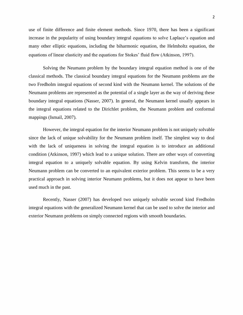
A Neumann problem is a boundary value problem for determining a harmonic function

yxu , interior or exterior to a region with prescribed values of its normal derivative n u on

the boundary.

Applications of Neumann problems abound in classical mathematical physics. Some

examples are heat problems in an insulated plate, electrostatic potential in a cylinder and

potential of flow around airfoil. If the region is a disk, exact solution formula for the Neumann

problem is known and the formula is called Dini‟s formula. For arbitrary simply connected

region, the solution formula requires conformal mapping.

A more direct approach that avoid conformal mapping is the boundary integral equation

method for solving the Neumann problem. Recently, Nasser (2007) has developed two integral

equations with the generalized Neumann kernel that can provide the boundary values of the

solution of the Neumann problem. Nasser‟s method is based on an earlier works by Murid and

Nasser (2003) and Wegmann et al. (2005) related to the Riemann problem and Dirichlet

problem.

1.3 Statement of the Problem

Through the previous research by Nasser (2007), the interior and exterior for Neumann

problems are reduced to equivalent Dirichlet problems by using Cauchy-Riemann equations and

it is uniquely solvable. Then, boundary integral equations are derived for the Dirichlet problems.

The question now arises whether it is possible to derive integral equations for Neumann

problems based on Murid and Nasser (2003) with the reduction to Riemann-Hilbert problems

using Cauchy-Riemann equations. This research has answered the question in affirmative.

4

1.4 Objectives of the Research

The objectives of this research are to:

i. study the Neumann problem and the Riemann-Hilbert problem as well as integral equations

for Riemann-Hilbert problem on multiply connected regions.

ii. reduce the interior and exterior Neumann problems to the equivalent Riemann-Hilbert

problems.

iii. derive the boundary integral equations related to the interior and exterior Riemann-Hilbert

problems.

iv. determine the solvability of the attained integral equations related to the Riemann-Hilbert

problems.

v. perform numerical calculations for solving the boundary integral equations using softwares

such as MATHEMATICA or MATLAB.

1.5 Importance of the Research

Knowledge on complex analysis in general and boundary integral equations in particular

is still growing. There have been several studies on boundary integral equations with Neumann

kernel related to Neumann problem. This research has developed non-singular integral equations

with continuous kernel associated to Neumann problem on multiply connected regions with

smooth boundaries. Furthermore, the analysis of solvability for these integral equations are

determined as well.

This approach has enriched the integral equation method for solving Neumann problem

and enhances the numerical effectiveness of solving it. Thus, the integral equation for Neumann

problem of this proposed research will assist scientists and engineers of our nation and abroad

working with mathematical models involving Neumann problem.

5

1.6 Scope of the Research

This research is mainly on the theoretical reduction of the Neumann problem to

Riemann-Hilbert problem. The Neumann problem is then solved numerically using the integral

equation related to Riemann-Hilbert problem. We are mainly concerned on the interior and

exterior Neumann problems on multiply connected regions with smooth boundaries.

1.7 Outline of Report

This project consists of seven chapters. The introductory Chapter 1 details some

discussion on the background of the problem, problem statement, objectives of research,

importance of the research, scope of the study and chapters organization.

Chapter 2 presents some auxiliary materials related to the Neumann problem, the

Riemann-Hilbert problems as well as integral equation for Riemann-Hilbert problems. In this

chapter, we reduce the interior Neumann problem into the interior Riemann-Hilbert problem and

construct the boundary integral equation for solving it. We discuss the question on how to treat

the integral equations numerically. Some numerical examples are presented to show the

effectiveness of the method.

Chapter 3 focuses on the development of a numerical method for the exterior Neumann

problem in a simply connected smooth region. Firstly, we reduce the exterior Neumann problem

to the exterior Riemann-Hilbert problem. Then, the boundary integral equation for the Neumann

problem is derived based on the exterior Riemann-Hilbert problem. Numerical implementations

of the derived integral equation are also presented.

In Chapter 4, we extend the results of Chapter 2 to reduce the Neumann problem to the

Riemann-Hilbert problem in multiply connected region, and then derive an integral equation with the

6

Neumann kernel related to the Riemann-Hilbert problem (briefly, RH problem). This integral equation is

the Fredholm integral equation of the second kind. Solvability of the integral equation is also discussed.

Numerical experiments on some test regions are also reported.

Chapter 5 deals with the reduction of exterior Neumann problem on a multiply connected

region to the exterior Riemann-Hilbert problem. Thus this chapter extends the results of Chapter

3. We show how to reduce the exterior Neumann problem on multiply connected region into the

exterior Riemann-Hilbert problem and derive the boundary integral equation for solving it. Then,

we provide a numerical technique for solving the boundary integral equation and present some

numerical examples on several test regions.

Finally the concluding Chapter 6 contains a summary of findings and achievements.

7

CHAPTER 2

AN INTEGRAL EQUATION METHOD FOR SOLVING NEUMANN PROBLEMS ON

SIMPLY CONNECTED SMOOTH REGIONS

2.1 Introduction

A Neumann problem is a boundary value problem of determining a harmonic function

interior or exterior to a region with prescribed values of its normal derivative on the boundary.

Applications of Neumann problems abound in classical mathematical physics. Some examples

are heat problems in an insulated plate, electrostatic potential in a cylinder, potential flow around

airfoil. If the region is a disk, exact solution formula for the Neumann problem is known and the

formula is called Dini‟s formula. For arbitrary simply connected region, the solution formula

requires conformal mapping. A more direct approach that avoid conformal mapping is the

boundary integral equation method for solving Neumann problem.

The boundary integral equation method is one of the classical methods for solving the

Neumann problem, see, for example, the books by Atkinson (1997) and Henrici (1986). Some

classical boundary integral equations for the Neumann problems are the Fredholm integral

equations of second kind with the Neumann kernel. These integral equations are derived by

8

representing the solutions of the Neumann problems as the potential of a single layer. However,

the integral equation for the interior Neumann problem is not uniquely solvable since the lack of

unique solvability for the Neumann problem itself. The simplest way to deal with the lack of

uniqueness in solving the integral equation is to introduce additional conditions (Atkinson,

1997).

Recently, Nasser (2007) proposes a new method to solve the interior and the exterior

Neumann problems in simply connected regions with smooth boundaries. The method is based

on two uniquely solvable Fredholm integral equations of the second kind with the generalized

Neumann kernel.

This chapter is organized as follows: Section 2.2 presents some auxiliary materials

related to the Neumann problem, the Riemann-Hilbert problems as well as integral equation for

Riemann-Hilbert problems. In Section 2.3, we reduce the interior Neumann problem into the

interior Riemann-Hilbert problem and construct the boundary integral equation for solving it. We

will discuss the question on how to treat the integral equations numerically in Section 2.4. Some

numerical examples are presented in Section 2.5. In Section 2.6, a short conclusion is given.

2.2 Auxiliary Material

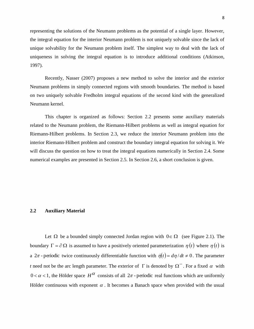
Let be a bounded simply connected Jordan region with 0 (see Figure 2.1). The

boundary is assumed to have a positively oriented parameterization t where t is

a periodic-2 twice continuously differentiable function with 0/ dtdt . The parameter

t need not be the arc length parameter. The exterior of is denoted by . For a fixed with

10 , the Hölder space H consists of all periodic-2 real functions which are uniformly

Hölder continuous with exponent . It becomes a Banach space when provided with the usual

9

Hölder norm. A Hölder continuous function h on can be interpreted via thth ˆ as a

Hölder continuous function h of the parameter t and vice versa.

Let tA be a continuous differentiable periodic-2 function with 0A . We define

two real kernels N and M by

)1.2(,Re1

,

t

t

tA

AtM

)2.2(.Im1

,

t

t

tA

AtN

The kernel tN , is called a generalized Neumann kernel formed with A and . When 1A ,

the kernel N is the Neumann kernel which arises frequently in the integral equations for potential

theory and conformal mapping.

Lemma 2.1 (Wegmann et al., 2005)

a) The kernel tN , is continuous with

)3.2(.2

1Im

1,

tA

tA

t

tttN

b) The kernel tM , has the representation

)4.2(,,2

cot2

1,

1tM

ttM

with the continuous kernel M1 which takes on the diagonal the values

)5.2(.2

1Re

1,

1

tA

tA

t

tttM

Let N and 1M be the Fredholm integral operators associate with the continuous kernels N and

M1, i.e.,

10

)6.2(,,2

0

dtttN

N

)7.2(.,2

0

1dtttM

1M

Let also M and K be the singular integral operators

)8.2(,,2

0

dtttM

M

)9.2(.2

cot2

1 2

0

dtt

t

K

The integrals in (2.8) and (2.9) are principal value integrals. The operator K is known as the

Hilbert transform. The operators N , M , 1M and K are bounded in H and map

H into H

. It follows from (2.4) that

)10.2(.KMM 1

Lemma 2.2 (Wegmann et al., 2005)

a) Let N be the generalized Neumann kernel formed with 1A and . Then 1 is not an

eigenvalue of N.

b) Let N be the generalized Neumann kernel formed with A and . Then 1 is not an

eigenvalue of N.

11

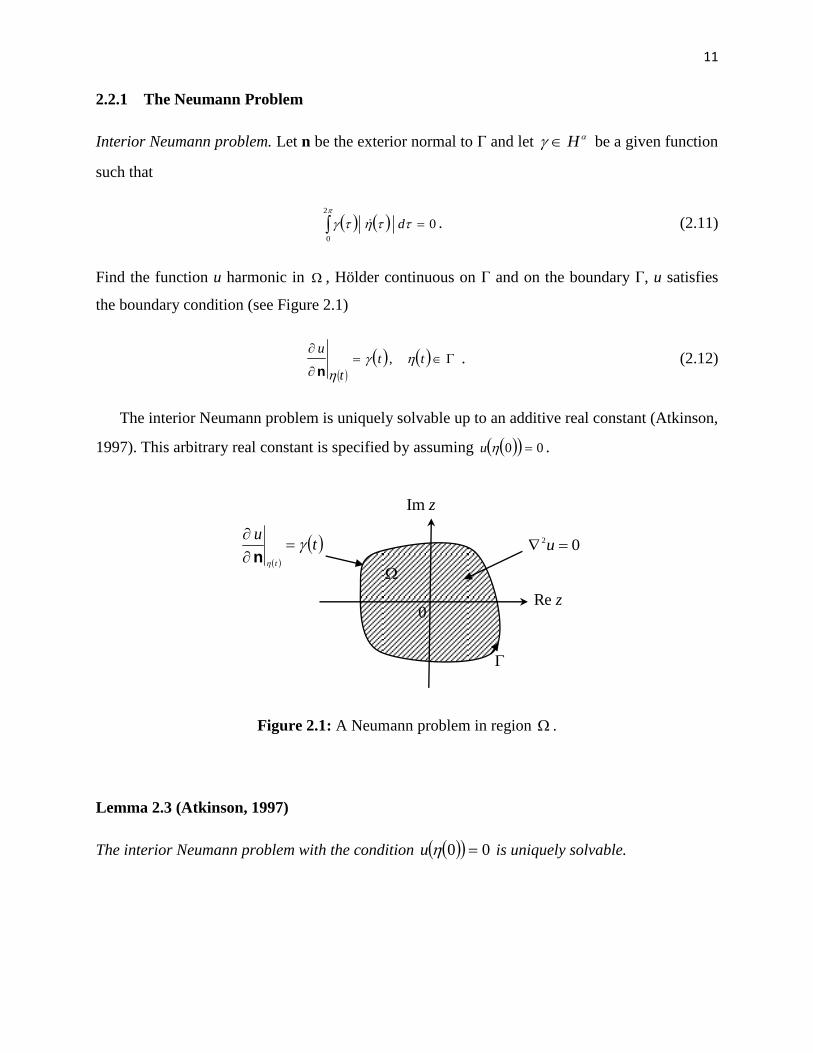
2.2.1 The Neumann Problem

Interior Neumann problem. Let n be the exterior normal to and let H be a given function

such that

2

0

0 d . (2.11)

Find the function u harmonic in , Hölder continuous on and on the boundary , u satisfies

the boundary condition (see Figure 2.1)

tt

t

u

,

n . (2.12)

The interior Neumann problem is uniquely solvable up to an additive real constant (Atkinson,

1997). This arbitrary real constant is specified by assuming 00 u .

tu

t

n

02 u

Figure 2.1: A Neumann problem in region .

Lemma 2.3 (Atkinson, 1997)

The interior Neumann problem with the condition 00 u is uniquely solvable.

z Re

z Im

0

12

2.2.2 The Riemann-Hilbert Problem

Interior Riemann-Hilbert problem. Let HC and A be given functions. Find a function F

analytic in , continuous on the closure , such that the boundary values F from inside

satisfy

tCtvtbtuta . (2.13)

Another frequently used form of writing the boundary condition is

).()()(,,Re tibtatAttCtFtAt

(2.14)

If 0tC , then this equation is a non-homogeneous boundary condition, while if 0tC , we

have a homogeneous boundary condition, i.e.,

. , 0 Re ttFtAt

(2.15)

Equation (2.13) is also equivalent to

, 2

tA

tCtF

tA

tAtF (2.16)

where

13

. tibtatA (2.17)

So, we call equation (2.14) as the non-homogeneous interior Riemann-Hilbert problem and

equation (2.15) as the homogeneous interior Riemann-Hilbert problem.

The solvability of the Riemann-Hilbert problem in a region depends upon the

geometry of the simply connected region with smooth boundary as well as upon the index of

the function )(tA with respect to the boundary which is denoted by

. ind A

(2.18)

It is also regarded as the index of the Riemann-Hilbert problem (Gakhov, 1966).

Suppose that is a smooth Jordan curve and tA is a continuous non-vanishing

function given on . The index of the function tA with respect to the curve is defined to be

the increment of its argument in traversing the curve in the positive direction, divided by 2 .

Then, the index of tA can be written in the form

. arg2

1ind

tAA

(2.19)

The index can be expressed by the integral

, ln 2

1 arg

2

1ind

tAd

itAdA

(2.20)

where the integral is understood in the sense of the Stieltjes (Gakhov, 1966). If the function tA

is continuously differentiable on , then

. 2

1ln

2

1ind dt

tA

tA

itAd

iA

(2.21)

Since is closed and tA is a non-vanishing continuous function on , the index A

ind is

an integer.

14

2.2.3 Integral Equation for Interior Riemann-Hilbert Problem

Theorem 2.1 (Wegmann et al., 2005)

If F is the solution of the interior Riemann-Hilbert problem (2.14) with boundary values

titCtFtA , (2.22)

then the imaginary part in (2.22) satisfies the integral equation

CMN . (2.23)

Theorem 2.2 (Wegmann et al., 2005)

a) If 0 then the integral equation

, N (2.24)

has a solution if and only if R ,where

. 0 , , Re: Gnanalytic iGtGtAtCHCR

b) If 0 then the integral equation (2.24) has a unique solution for anyH .

c) Equation (2.23) is solvable for each HC .

15

2.3 Reduction of the Neumann Problem to the Riemann-Hilbert Problem

Suppose that u is a solution of the interior Neumann problem. Since u is harmonic

function in , then u has a harmonic conjugate v in . Then ivuf is analytic in

with derivative

xx ivuf ' . (2.25)

The directional derivative of f in the direction of the outer unit normal vector to the path

is given by (Husin, 2009)

t

vi

u

t

f

nnn

. (2.26)

Assuming tiytxt and applying

n

n

u

u and

jy

ix

jt

txi

t

ty

nnn

'

'

, we obtain

tyy

iuy

vixx

ivx

u

t

f

nn

n

. (2.27)

Applying (2.25) and Cauchy-Riemann equations, we get

ty

ix

f

t

f

nn

n' . (2.28)

Taking the real parts of both sides and applying (2.12), the above equation becomes

tft

' Re n . (2.29)

16

After substituting

t

ti

n into (2.29), we get

' Re

ttftitt

. (2.30)

Letting ' fig and ttt we obtain

tt

tgt

Re , (2.31)

which is the interior Riemann-Hilbert problem. Comparison of (2.31) with (2.14) yields

, ttA , tgtF and )()( ttC .

2.3.1 Integral Equation for Solving Interior Neumann Problem

By Theorem 2.1, if tg is the solution of the interior Riemann–Hilbert problem (2.31)

with boundary values

tittgt , (2.32)

then the imaginary part in (2.32) satisfies the integral equation

MN , (2.33)

i.e.

.2

0

,2

0

,

dtttMdtttN (2.34)

17

The solvability of the Riemann-Hilbert problem (2.31) is determined by the index of the

function tA which is defined as the winding number of A with respect to 0 . Applying

(2.21) with tA , we get

.1

2

1

tdti

(2.35)

By means of the Cauchy Integral Formula, we get 1 .

Thus, by Theorem 2.2, integral equation (2.33) has a unique solution for HM and

integral equation (2.33) is solvable for each HC .

2.4 Numerical Implementation

Since the functions tA and t are periodic2 - , the integral operator N in

(2.6) can be best discretized on an equidistant grid by the trapezoidal rule, i.e., the integral

operator N is discretized by the Nyström method (Atkinson, 1997).

Define the n equidistant collocation points i

t by

. ..., ,2 ,1 , 2

1 nin

iti

(2.36)

Then, using the Nyström method with the trapezoidal rule to discretize the integral equation

(2.33), we obtain the linear system

, i

n

jjnjiin ttttN

nt

M

1

,2

(2.37)

for n, i ..., ,21 where n is an approximation to . Note that the kernels N and M in (2.37)

are formed with A .

18

Defining the matrix ][ ijQQ and vector ][ ixx and ][ iyy by

i

ti

yi

tnix

jt

itN

nijQ , , ,

2

M

,

equation (2.37) can be rewritten as an n by n system

yx QI . (2.38)

For the calculation on the right-hand side of (2.37), we first calculate

. ..., , n ittt iii ,2,1 (2.39)

Then, by using (2.10), we have

iii ttt KMM 1 (2.40)

for n, i ..., ,21 . The values of i

t K will be calculated directly by using

MATHEMATICA package, i. e., CauchyPrincipalValue, while the values of it 1M will

be calculated by using the trapezoidal rule, i. e.,

,,2

111

n

jjjii tttM

nt

M (2.41)

for n, i ..., ,21 . Finally, (2.32) implies

iniii tittfti ' .

Clearly the equation gives the solution of the Neumann problem since ivuf . By

obtaining 'f , we can obtain the function f by the Fundamental Theorem of Complex Integration

which in turn gives the solution u of the Neumann problems.

19

2.5 Examples

Example 2.1

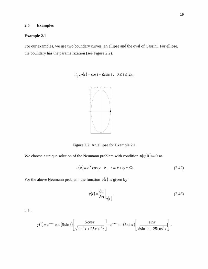
For our examples, we use two boundary curves: an ellipse and the oval of Cassini. For ellipse,

the boundary has the parametrization (see Figure 2.2).

πttitt 20 , sin5cos:1

,

Figure 2.2: An ellipse for Example 2.1

We choose a unique solution of the Neumann problem with condition 00 u as

iyxzeyxezu , cos . (2.42)

For the above Neumann problem, the function t is given by

t

ut

n. (2.43)

i. e.,

tt

tte

tt

ttet tt

22

cos

22

cos

cos25sin

sinsin5sin

cos25sin

cos5sin5cos .

0

1

2

3

4

5 -1 -0.5 0 0.5 1

20

We now give a verification of (2.31).

ttettettt tt sin5sinsinsin5coscos5 coscos .

Now, we consider the left-hand side of equation (2.31) for the same region. We define the

analytic function as

yxivyxuyxfzf ,),(, ,

where yeyxv xsin),( is a harmonic conjugate of eyeyxu x cos),(

tieetetf tt sin5sinsin5cos coscos . (2.44)

Thus

tieteivutf tt

txx sin5sinsin5cos' coscos

. (2.45)

Multiplying this result with it , we have

tietetittfit tt sin5cossin5sincos5sin' coscos .

Therefore, the left-hand side of equation (2.31) is

21

which is equal to the right-hand side of (2.31). This completes the verification.

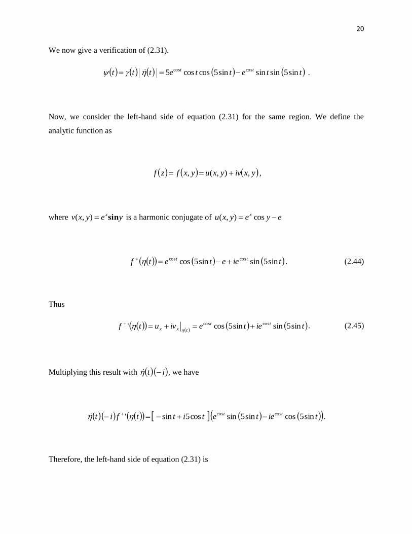
Example 2.2

For the oval of Cassini, the boundary parametrization is

πtitetRt 20 , :2

,

where ttR 2cos25.2 (see Figure 2.3).

Figure 2.3: An oval of Cassini for Example 2.2

We again choose the unique solution of the Neumann problem with condition 00 u as

iyxzeyezu x ,cos . (2.46)

For this problem, the unit tangent vector t

ttT

, i. e.,

[

[

]sin)('cos)(cos)('sin)(

]sin)('cos)(cos)('sin)(

ttRttRittRttR

ttRttRittRttR

t

ttT

.

For the above Neumann problem, the function t is given by,

-1

0

1

-4 -3 -2 -1 0 1 2 3 4

,sin5 sinsin sin5 coscos5 ' Re coscos ttettetfit tt

22

,

''

)(

t

txutyuut

yx

n (2.47)

i.e.,

. [

[

]sin)('cos)(cos)('sin)(

cos)('sin)(sinsin

]sin)('cos)(cos)('sin)(

sin)('cos)(sincos

cos

cos

ttRttRittRttR

ttRttRttRe

ttRttRittRttR

ttRttRttRet

ttR

ttR

We now give a verification of (2.31). The right-hand side of equation (2.31) for the second

region is

.

ttRttRttRe

ttRttRttRettt

ttR

ttR

cos'sinsinsin

sin'cossincos

cos

cos

Now, we consider the left-hand side of equation (2.31) for the same region. Thus

ttRiettReivutf ttRttR

txx sinsinsincos' coscos

. (2.48)

Multiplying the result with it , we have

.sin sinsin cos

sin'cos cos'sin ' cos cos ttRettRie

ttRttRittRttRtfitttRttR

Therefore, the left-hand side of equation (2.31) is

23

,

ttRttRttRe

ttRttRttRetfit

ttR

ttR

cos'sinsinsin

sin'cossincos'Re

cos

cos

which is equal to the right-hand side (2.31). This completes the verification.

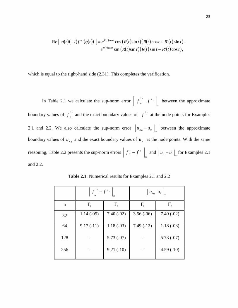
In Table 2.1 we calculate the sup-norm error

''

ff n

between the approximate

boundary values of fn

'

and the exact boundary values of f'

at the node points for Examples

2.1 and 2.2. We also calculate the sup-norm error

xnx uu between the approximate

boundary values of nxu and the exact boundary values of xu at the node points. With the same

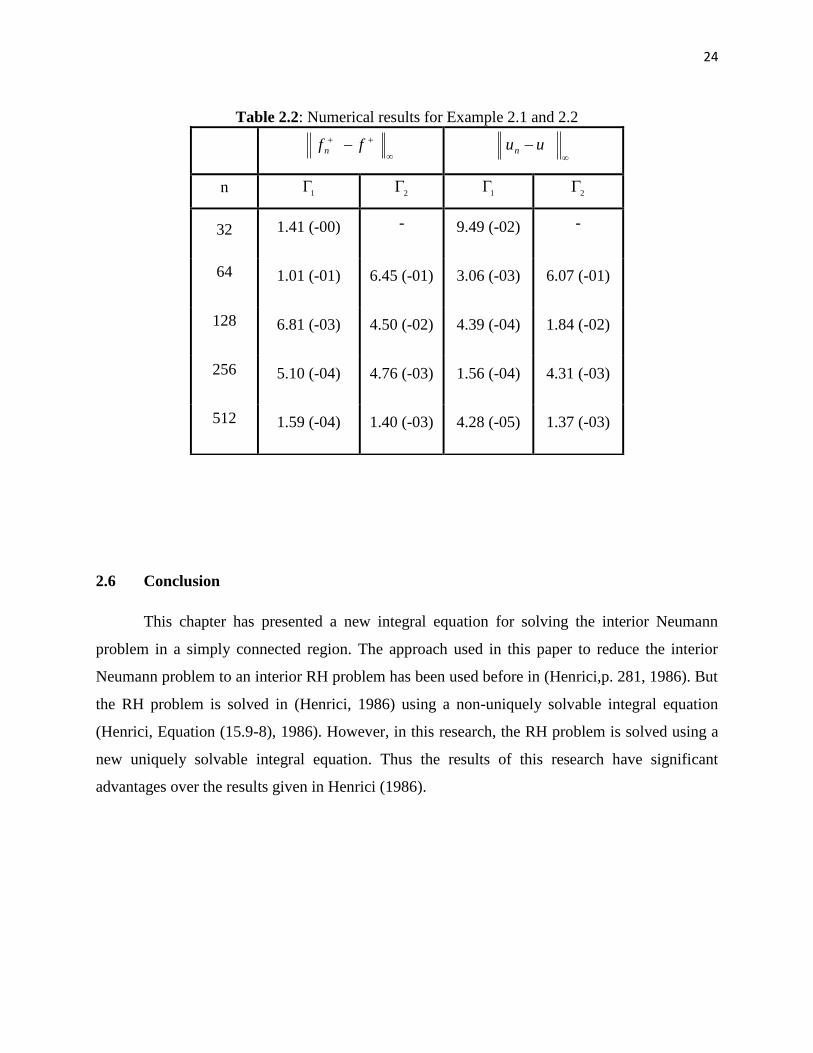
reasoning, Table 2.2 presents the sup-norm errors

ff n and

uun for Examples 2.1

and 2.2.

Table 2.1: Numerical results for Examples 2.1 and 2.2

'' ff

n

xnx uu

n 1

2

1

2

32 1.14 (-05) 7.40 (-02) 3.56 (-06) 7.40 (-02)

64 9.17 (-11) 1.18 (-03) 7.49 (-12) 1.18 (-03)

128 - 5.73 (-07) - 5.73 (-07)

256 - 9.21 (-10) - 4.59 (-10)

24

Table 2.2: Numerical results for Example 2.1 and 2.2

2.6 Conclusion

This chapter has presented a new integral equation for solving the interior Neumann

problem in a simply connected region. The approach used in this paper to reduce the interior

Neumann problem to an interior RH problem has been used before in (Henrici,p. 281, 1986). But

the RH problem is solved in (Henrici, 1986) using a non-uniquely solvable integral equation

(Henrici, Equation (15.9-8), 1986). However, in this research, the RH problem is solved using a

new uniquely solvable integral equation. Thus the results of this research have significant

advantages over the results given in Henrici (1986).

ffn

uun

n 1

2

1

2

32 1.41 (-00) - 9.49 (-02) -

64 1.01 (-01) 6.45 (-01) 3.06 (-03) 6.07 (-01)

128 6.81 (-03) 4.50 (-02) 4.39 (-04) 1.84 (-02)

256 5.10 (-04) 4.76 (-03) 1.56 (-04) 4.31 (-03)

512 1.59 (-04) 1.40 (-03) 4.28 (-05) 1.37 (-03)

25

CHAPTER 3

AN INTEGRAL EQUATION METHOD FOR SOLVING EXTERIOR NEUMANN

PROBLEMS ON SIMPLY CONNECTED SMOOTH REGIONS

3.1 Introduction

In Chapter 2, the interior Neumann problem is reduced to equivalent Riemann-Hilbert

problem by using Cauchy-Riemann equations. The boundary integral equation is then derived for

the Riemann-Hilbert problem based on an earlier work by Nasser (2007).

This chapter will focus on the development of a numerical method for the exterior

Neumann problem in a simply connected smooth region. Firstly, the exterior Neumann problem

will be reduced to the exterior Riemann-Hilbert problem. Then, the boundary integral equation

for the Neumann problem will be derived based on the exterior Riemann-Hilbert problem.

The organization of this chapter is as follows. We present some auxiliary materials in

Section 3.2. In Section 3.3, we show how to construct our new integral equation for the

exterior Neumann problem based on the exterior Riemann-Hilbert problem. In Section 3.4 we

discuss the numerical implementations of the derived integral equation. Finally, a short

conclusion is given in Section 3.5.

26

3.2 Auxiliary Material

Let be a bounded simply connected Jordan region bounded by and let the exterior

of be denoted by with 0 and belongs to . The boundary : is assumed

to have a positively oriented parametrization )(t where )(t is a periodic2 twice

continuously differentiable function with 0)( dt

dt

. The parameter t need not be the arc

length parameter. Let be a real-valued function defined on .

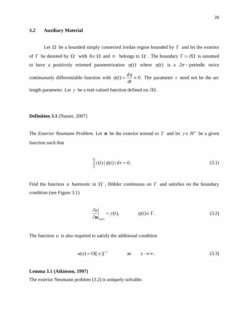
Definition 3.1 (Nasser, 2007)

The Exterior Neumann Problem. Let n be the exterior normal to and let H be a given

function such that

0|)(|)(2

0

dtt . (3.1)

Find the function u harmonic in , Hölder continuous on and satisfies on the boundary

condition (see Figure 3.1)

.)(),()(

tt

u

t

n

(3.2)

The function u is also required to satisfy the additional condition

.as|)(|)( 1 zzOzu (3.3)

Lemma 3.1 (Atkinson, 1997)

The exterior Neumann problem (3.2) is uniquely solvable.

27

Figure 3.1: The exterior Neumann Problem

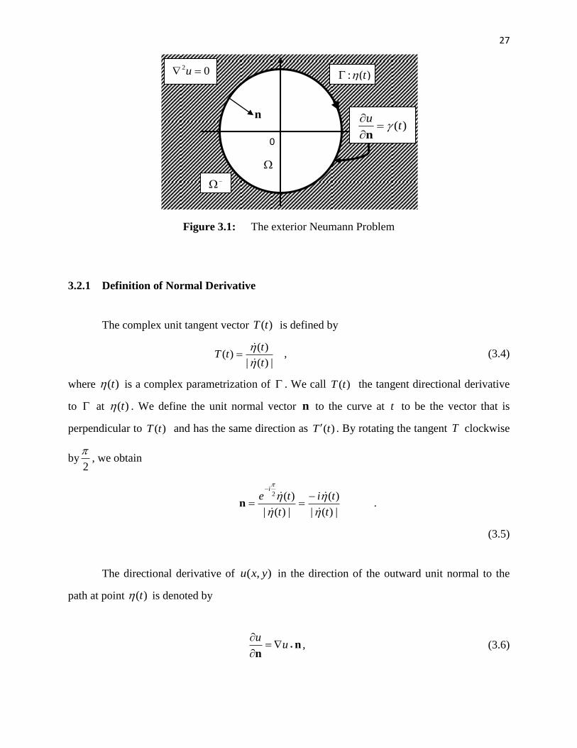
3.2.1 Definition of Normal Derivative

The complex unit tangent vector )(tT is defined by

|)(|

)()(

t

ttT

, (3.4)

where )(t is a complex parametrization of . We call )(tT the tangent directional derivative

to at )(t . We define the unit normal vector n to the curve at t to be the vector that is

perpendicular to )(tT and has the same direction as )(tT . By rotating the tangent T clockwise

by2

, we obtain

|)(|

)(

|)(|

)(2

t

ti

t

tei

n .

(3.5)

The directional derivative of ),( yxu in the direction of the outward unit normal to the

path at point )(t is denoted by

nn

u

u, (3.6)

)(: t

n

0

)(tu

n

02 u

28

where juiuyxu yx

).( . If )()()( tiytxt is the parametrization of , then

)()()( tyitxt . Therefore, (3.5) becomes

jijt

txi

t

ty

t

tyitxiyx

nnn

|)(|

)(

|)(|

)(

|)(|

))()((

. (3.7)

Substituting (3.7) into (3.6), we obtain

|)(|

)()(

t

txutyuu yx

n. (3.8)

3.2.2 The Exterior Riemann-Hilbert (RH) Problem

Definition 3.2 (Zamzamir et al.,2009)

The Exterior RH Problem. Given functions A and C , it is required to find a function g analytic

in and continuous on the closure

with 0)( g such that the boundary values g

satisfy

)(),())](()(Re[ ttCtgtA . (3.9)

The boundary condition (3.9) can be written in the equivalent form

.)(,)(

)(2))((

)(

)())(( t

tA

tCtg

tA

tAtg (3.10)

The homogenous boundary condition of the exterior RH problem is given by

29

.)(,0))](()(Re[ ttgtA (3.11)

The solvability of the RH problem is determined by the index of the function A . The

index of the function A is defined as the winding number of A with respect to zero. If the

function )(tA is continuously differentiable on , then

dt

tA

tA

itAd

iA

)(

)(

2

1)(ln

2

1)(ind

. (3.12)

The number of arbitrary real constants in the solutions of the homogenous RH problems,

i.e. )dim( S and the number of conditions on the function C so that the non-homogenous RH

problems are solvable, i.e. )(codim R are given in term of the index as in the following

theorem from Wegmann et al. (2005).

Theorem 3.1.

The codimensions of the spaces R and the dimensions of the spaces S are given by the

formulas

.)12,0max()dim(

),12,0max()(codim

S

R

30

3.2.3 Integral Operators

Let )(tA be a continuously differentiable periodic2 function with 0A . We define

two real functions N and M by

.)()(

)(

)(

)(Re

1:),(

,)()(

)(

)(

)(Im

1:),(

t

t

tA

AtM

t

t

tA

AtN

We also define the kernels U and V (when 1A for the kernels N and M ) as

.)()(

)(Re

1:),(

,)()(

)(Im

1:),(

t

ttU

t

ttV

We then define the kernels *U and *V (the adjoint kernels of U and V ) as

.)()(

)(Re

1:),(

,)()(

)(Im

1:),(

*

*

ttU

ttV

31

Lemma 3.2 (Wegmann et al., 2005).

(a) The kernel ),( tN is continuous with

)(

)(

)(

)(

2

1Im

1),(

tA

tA

t

ttN

.

(b) The kernel ),( tM has representation ),(2

cot2

1),(

1tM

ttM

with a continuous

kernel 1

M which takes on the diagonal the values

)(

)(

)(

)(

2

1Re

1:),(

1tA

tA

t

ttM

.

3.2.4 Integral Equation for the Exterior Riemann-Hilbert Problem

For a given function HC , , let the function )(z be defined by

.,)(

)()(

2

1)(

z

z

d

A

iC

iz

(3.13)

Based on the application of Plemelj‟s formula, a boundary integral equation with generalized

Neumann kernel has been derived for exterior RH problem by Wegmann et al. (2005), as in the

following theorem.

Theorem 3.2

If )(zg is a solution of the exterior problem (3.9) with boundary values

)()())(()( titCtgtA (3.14)

then the imaginary part in (3.14) satisfies the integral equation

32

.CMN (3.15)

By Theorem 3.2, if ))(( tg is the solution of the exterior Riemann-Hilbert problem with

boundary values

),()())(()( tittgt (3.16)

then the imaginary part in (3.16) satisfies the integral equation

, MN (3.17)

i.e.

.)(),()(),()(2

0

2

0

dtttMdtttN (3.18)

The next theorem represents the solvability of the integral equation (3.15).

Theorem 3.3 (Zamzamir et al., 2009)

If 0 , then the integral equation (3.15) is uniquely solvable. If 0 , then the integral

equation (3.15) is non-uniquely solvable.

33

3.3 Modification of the Exterior Neumann Problem

3.3.1 Reduction of the Exterior Neumann Problem to the RH Problem

Suppose that u is the solution of the exterior Neumann problem and v is a harmonic

conjugate of u in . The function ),(),()( yxivyxuzf is analytic in where

jtyitxtiytxt

)()()()()(: if and only if the partial derivatives of u and v are

continuous and satisfy the Cauchy-Riemann equations. The directional derivative of f in the

direction of the outer unit normal vector to the path is given by

)()(

)(

tt

vi

uf

nnn. (3.19)

Using the concept of normal derivative and Cauchy-Riemann equation, we obtain

)()(

))(()(

tyx

t

iff

nnn

. (3.20)

Therefore, we can write (3.2) as the real part of (3.20),

)(])()(Re[)(

tiftyx

nn . (3.21)

Substituting (3.7) and (3.5) into (3.21), we get

).()()(

)(Re)(Re

)(tf

t

tif

t

n (3.22)

Letting ))(())(( tfitg and )()()( ttt , we obtain

34

)())](()(Re[ ttgt (3.23)

which is the exterior RH problem as defined in Section 3.2.2. Comparison of (3.23) with (3.9)

yields )()( ttA and )()( ttC .

By Theorem 3.2, if )(zg is a solution of the exterior problem (3.23) with boundary

values )()())(()( tittgt , then the imaginary part satisfies the integral equation

MN . (3.24)

Applying (3.12) with )()( ttA , we obtain 1 . From Theorem 3.1, we obtain

0)codim( -R which means that the non-homogenous exterior RH problem is solvable and

1)dim( S implies that the solution of the exterior RH problem is not unique. Also from

Theorem 3.3, we conclude that the integral equation (3.24) is non-uniquely solvable. The

approach to overcome the non-uniqueness is discussed in the following section.

3.3.2 Modified Integral Equation for the Exterior RH Problem

With )()( ttA , the kernel N becomes ),(),( * tVtN while the kernel M

becomes ),(),( * tUtM . Therefore, the non-uniquely solvable integral equation (3.24)

become

**UV . (3.25)

Recall from Section 3.1 that the function f is analytic on . Then at each point z

in that domain when )(,00 zfz can be represented by the following Laurent series expansion

such that 0)( f :

35

3

3

2

21)(z

c

z

c

z

czf (3.26)

Differentiate once respect to z and multiply with iz , we obtain

)(32

)(3

3

2

21 zFz

c

z

c

z

czfzi (3.27)

Therefore,z

zFtg

)())(( since ))(())(( tfitg . By means of Cauchy Integral Formula,

we obtain

.0)(

dg (3.28)

Notice that, )(

)()())((

t

tittg

, so (3.28) becomes

.0)()(2

0

2

0

dttidtt (3.29)

Note that, the exterior Neumann problem need to satisfy (3.1). With )()()( ttt , (3.1)

becomes 0)(

2

0

dtt which is the additional condition for the exterior RH problem which the

right-hand side of the RH problem needs to satisfy. Thus (3.29) becomes

0)(

2

0

dtt . (3.30)

Let the kernel ),( t be defined as

2

1),( t and let the operator J be defined by

36

2

0

2

0

)(2

1)(),()( dttdttttJ . (3.31)

Therefore, we can write (3.30) as (3.31) where 0)(2

1)(

2

0

dtttJ . Adding this integral

equation with our integral equation (3.25) yields the new integral equation

**UJV . (3.32)

According to Mikhlin (1957), this new integral equation (3.32) is uniquely solvable. The proof of

the solvability of the integral equation can be followed from the paper written by Atkinson

(1967).

From Lemma 3.2, we can write the kernel of the right-hand side of (3.32) as

),(),(* tMtU which is singular since it is unbounded when t . To remove the

difficulty, we will use the function ),( tB defined in Wegmann et al. (2005), with )()( ttA

where

.for,)(

)(Re)()(

1

,for,)()(

)()()()(Re

1

),(

tt

tt

tt

tt

tB

(3.33)

Therefore, our uniquely solvable integral equation (3.32) becomes

BJV* (3.34)

where .),(2

0

dttBB

37

By obtaining , the Cauchy integral formula implies that the function )(zf can be calculated

for z by

2

0 )(

)(

)(

)()(

2

1)(

2

1)(

zt

dtt

ti

tit

id

z

f

izf

(3.35)

and the function )(zf can be expressed as an anti-derivative function of )(zf for z . So

we have

.)()(

1log)(

)()(

2

1)(

2

0

dttz

t

ti

tit

izf

(3.36)

3.4 Numerical Implementations of the Boundary Integral Equation

Since the function )()( ttA and )(t are periodic2 , the integrals in the integral

equation (3.34) can be best discretized by the Nyström method with the trapezoidal rule as the

quadrature rule (Atkinson, 1997). Let n be a given integer and define the n equidistant

collocation points kt by

.,,2,1,2

)1( nkn

ktk

(3.37)

Then, using the Nyström method with the trapezoidal rule to discretized the integral equation

(3.34), we obtain the linear system

n

k

n

kkjknkjknkj

n

kjn ttB

ntttJ

ntttV

nt

1 11

),(2

)(),(2

)(),(*2

)(

(3.38)

with nj ,,2,1 and n is an approximation to .

38

Let I be the nn identity matrix. Also let 11I and 1I be the nn matrix and 1n

vector whose elements are all unity. Define the matrices ][][][kjkjkj

BBJJV ,,V and

vectors ][],[ kk yyxx by

jk

j

j

jk

jk

k

jkkj

ttt

t

tttt

t

ntt

n,

)(

)(

2

1

,)()(

)(Im

1

2),(

2

*VV , (3.39)

11112

12),(

2IIJ

ntt

njkkjJ , (3.40)

jk

j

j

jj

jk

kj

kjjk

jkkj

ttt

ttt

tttt

tttt

ntt

n,

)(

)(Re)()(

1

,)()(

)()()()(Re

1

2),(

2

BB , (3.41)

),( knk tx (3.42)

1Ikjk By . (3.43)

Hence, the application of Nyström method to the uniquely solvable integral equations

(3.34) leads to the following n by n linear system

yxJVI )( . (3.44)

By solving the linear system (3.44), we obtain )( kn t for nk ,,2,1 . Then the

approximate solution )(tn can be calculated for all ]2,0[ t using the Nyström interpolating

formula, i.e., the approximation )(tn of the integral equation (3.34) is given by

n

j

jn

n

j

jnj

n

j

jn tn

tttVn

ttBn

t11

*

1

)(2

12)(),(

2),(

2)(

. (3.45)

By obtaining ,(3.35) and (3.36) implies that )(zf and )(zf can be calculated for z .

39

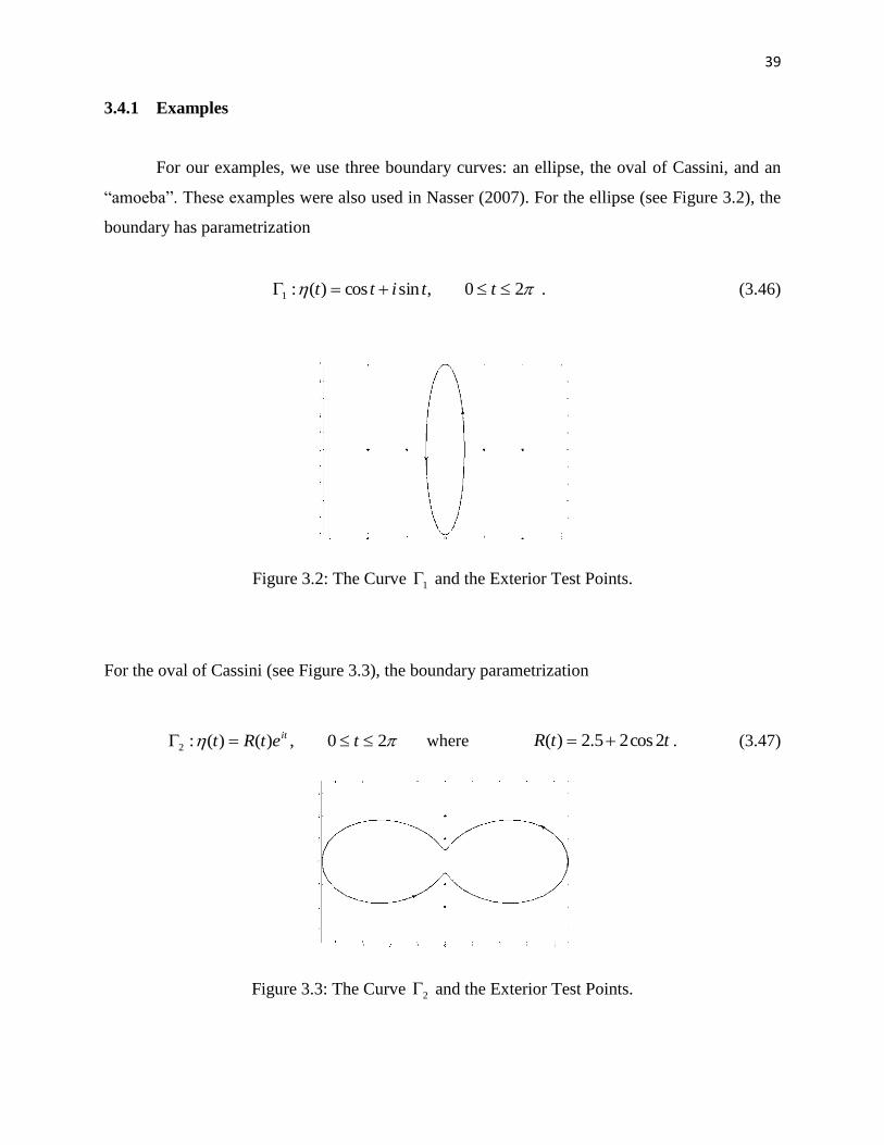
3.4.1 Examples

For our examples, we use three boundary curves: an ellipse, the oval of Cassini, and an

“amoeba”. These examples were also used in Nasser (2007). For the ellipse (see Figure 3.2), the

boundary has parametrization

20,sincos)(:1 ttitt . (3.46)

Figure 3.2: The Curve 1 and the Exterior Test Points.

For the oval of Cassini (see Figure 3.3), the boundary parametrization

20,)()(:2 tetRt it where ttR 2cos25.2)( . (3.47)

Figure 3.3: The Curve 2 and the Exterior Test Points.

40

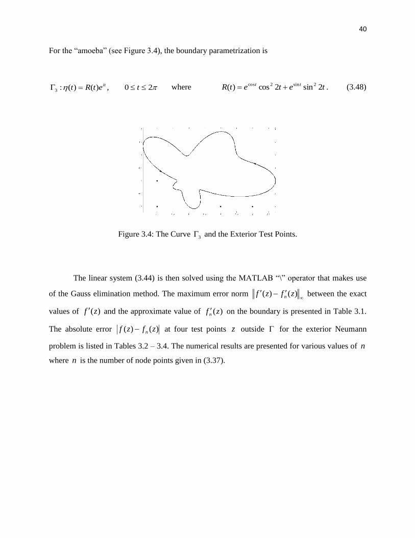
For the “amoeba” (see Figure 3.4), the boundary parametrization is

20,)()(:3 tetRt it where tetetR tt 2sin2cos)( 2sin2cos . (3.48)

Figure 3.4: The Curve 3 and the Exterior Test Points.

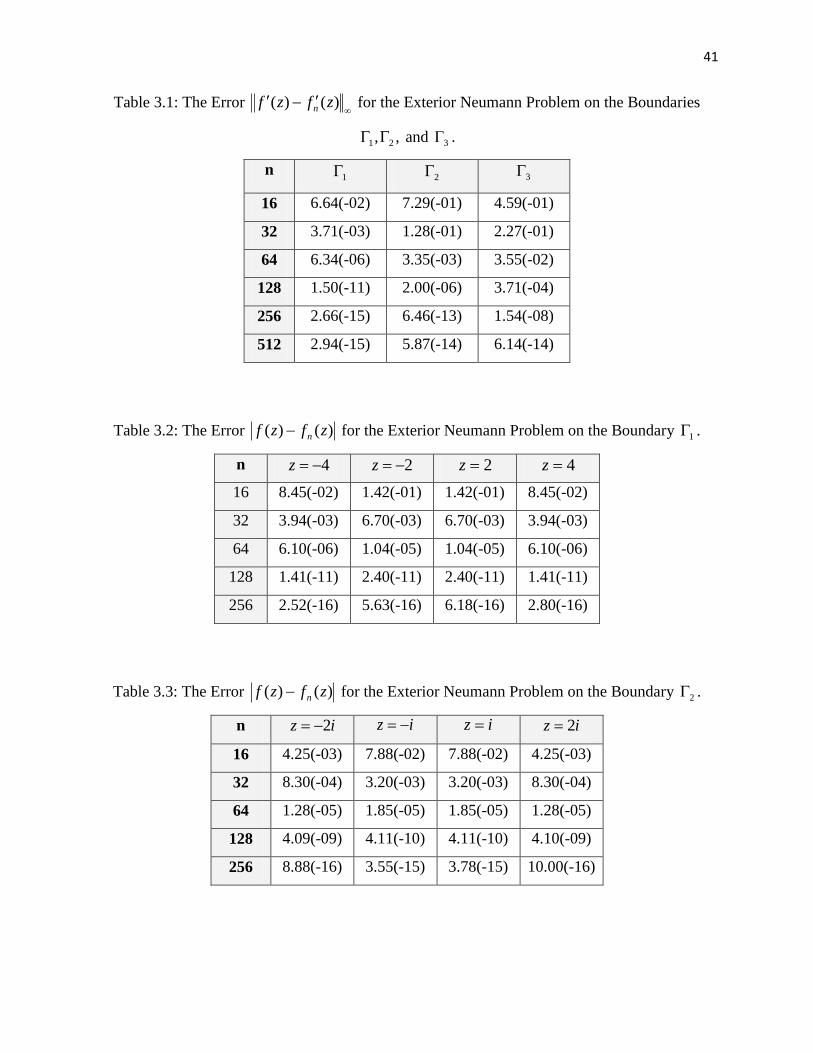
The linear system (3.44) is then solved using the MATLAB “\” operator that makes use

of the Gauss elimination method. The maximum error norm

)()( zfzf n between the exact

values of )(zf and the approximate value of )(zf n on the boundary is presented in Table 3.1.

The absolute error )()( zfzf n at four test points z outside for the exterior Neumann

problem is listed in Tables 3.2 – 3.4. The numerical results are presented for various values of n

where n is the number of node points given in (3.37).

41

Table 3.1: The Error

)()( zfzf n for the Exterior Neumann Problem on the Boundaries

,, 21 and 3 .

n 1 2 3

16 6.64(-02) 7.29(-01) 4.59(-01)

32 3.71(-03) 1.28(-01) 2.27(-01)

64 6.34(-06) 3.35(-03) 3.55(-02)

128 1.50(-11) 2.00(-06) 3.71(-04)

256 2.66(-15) 6.46(-13) 1.54(-08)

512 2.94(-15) 5.87(-14) 6.14(-14)

Table 3.2: The Error )()( zfzf n for the Exterior Neumann Problem on the Boundary 1 .

n 4z 2z 2z 4z

16 8.45(-02) 1.42(-01) 1.42(-01) 8.45(-02)

32 3.94(-03) 6.70(-03) 6.70(-03) 3.94(-03)

64 6.10(-06) 1.04(-05) 1.04(-05) 6.10(-06)

128 1.41(-11) 2.40(-11) 2.40(-11) 1.41(-11)

256 2.52(-16) 5.63(-16) 6.18(-16) 2.80(-16)

Table 3.3: The Error )()( zfzf n for the Exterior Neumann Problem on the Boundary 2 .

n iz 2 iz iz iz 2

16 4.25(-03) 7.88(-02) 7.88(-02) 4.25(-03)

32 8.30(-04) 3.20(-03) 3.20(-03) 8.30(-04)

64 1.28(-05) 1.85(-05) 1.85(-05) 1.28(-05)

128 4.09(-09) 4.11(-10) 4.11(-10) 4.10(-09)

256 8.88(-16) 3.55(-15) 3.78(-15) 10.00(-16)

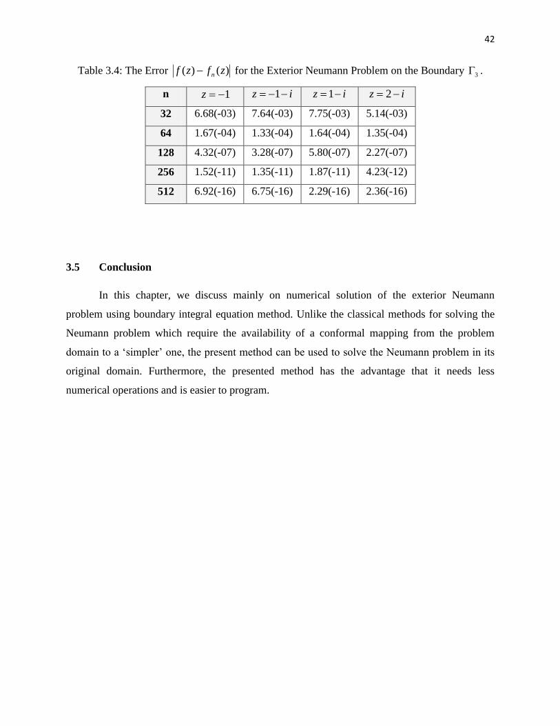
42

Table 3.4: The Error )()( zfzf n for the Exterior Neumann Problem on the Boundary 3 .

n 1z iz 1 iz 1 iz 2

32 6.68(-03) 7.64(-03) 7.75(-03) 5.14(-03)

64 1.67(-04) 1.33(-04) 1.64(-04) 1.35(-04)

128 4.32(-07) 3.28(-07) 5.80(-07) 2.27(-07)

256 1.52(-11) 1.35(-11) 1.87(-11) 4.23(-12)

512 6.92(-16) 6.75(-16) 2.29(-16) 2.36(-16)

3.5 Conclusion

In this chapter, we discuss mainly on numerical solution of the exterior Neumann

problem using boundary integral equation method. Unlike the classical methods for solving the

Neumann problem which require the availability of a conformal mapping from the problem

domain to a „simpler‟ one, the present method can be used to solve the Neumann problem in its

original domain. Furthermore, the presented method has the advantage that it needs less

numerical operations and is easier to program.

43

CHAPTER 4

A BOUNDARY INTEGRAL EQUATION FOR THE INTERIOR NEUMANN PROBLEM

ON BOUNDED MULTIPLY CONNECTED REGION

4.1 Introduction

Neumann problem is classified as a boundary value problem associated with Laplace‟s

equation and Neumann boundary condition. Different types of Neumann problems occur

naturally in some fields like electrostatics, fluid flow, heat flow and elasticity.

Boundary integral equation method is one of the common methods for solving Neumann

problem. This method reduces the task to solve an integral equation only on the boundary of the

region, thus reducing the dimension of the Neumann problem by one. Numerical treatment is

usually needed to solve the resulting integral equation. One example of such approach is given in

Nasser (2007) where the Neumann problem is reduced to a Dirichlet problem from which an

integral equation is constructed. In this chapter, we extend the results of Chapter 2 to reduce the

Neumann problem to the Riemann-Hilbert problem in multiply connected region, and then

derive an integral equation with the Neumann kernel related to the Riemann-Hilbert problem

(briefly, RH problem). This integral equation is the Fredholm integral equation of the second

kind.

44

4.2 Auxiliary Material

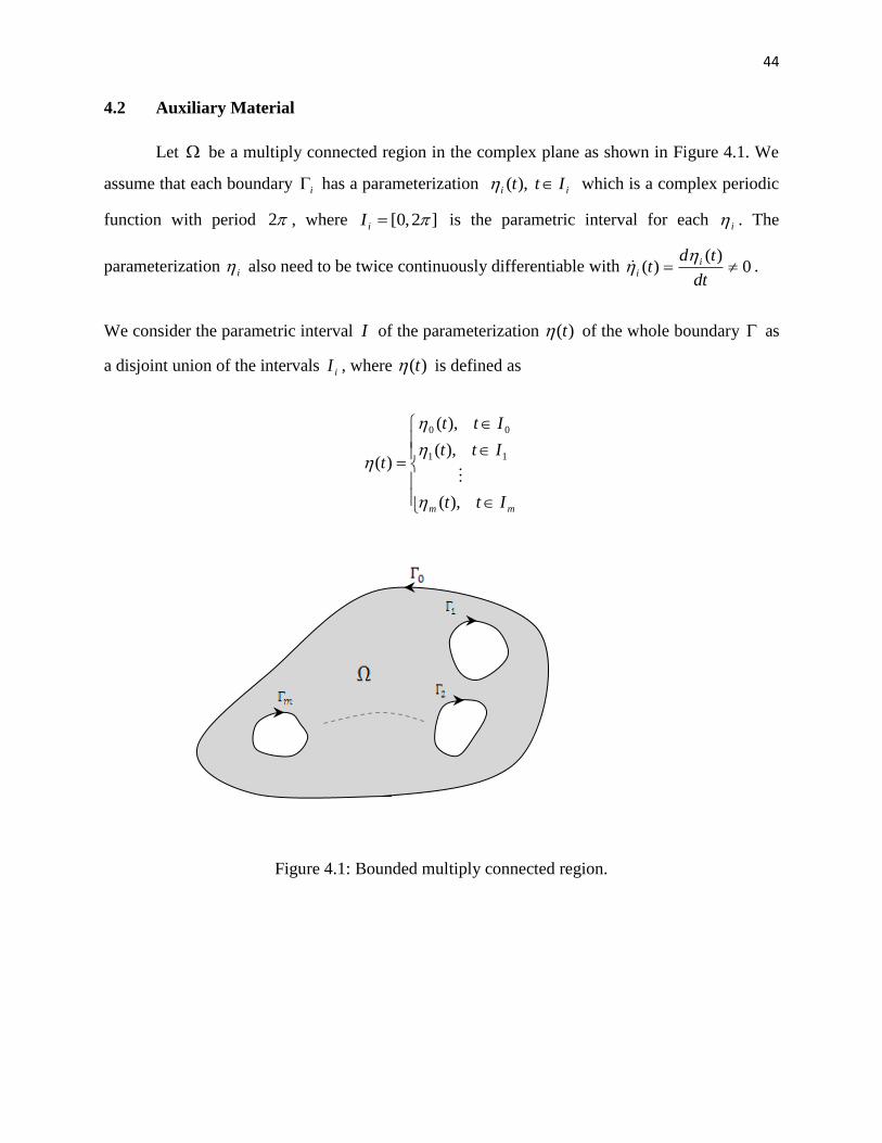
Let be a multiply connected region in the complex plane as shown in Figure 4.1. We

assume that each boundary i has a parameterization ii Itt ),( which is a complex periodic

function with period 2 , where ]2,0[ iI is the parametric interval for each i . The

parameterization i also need to be twice continuously differentiable with 0)(

)( dt

tdt i

i

.

We consider the parametric interval I of the parameterization )(t of the whole boundary as

a disjoint union of the intervals iI , where )(t is defined as

mm Itt

Itt

Itt

t

),(

),(

),(

)(11

00

Figure 4.1: Bounded multiply connected region.

45

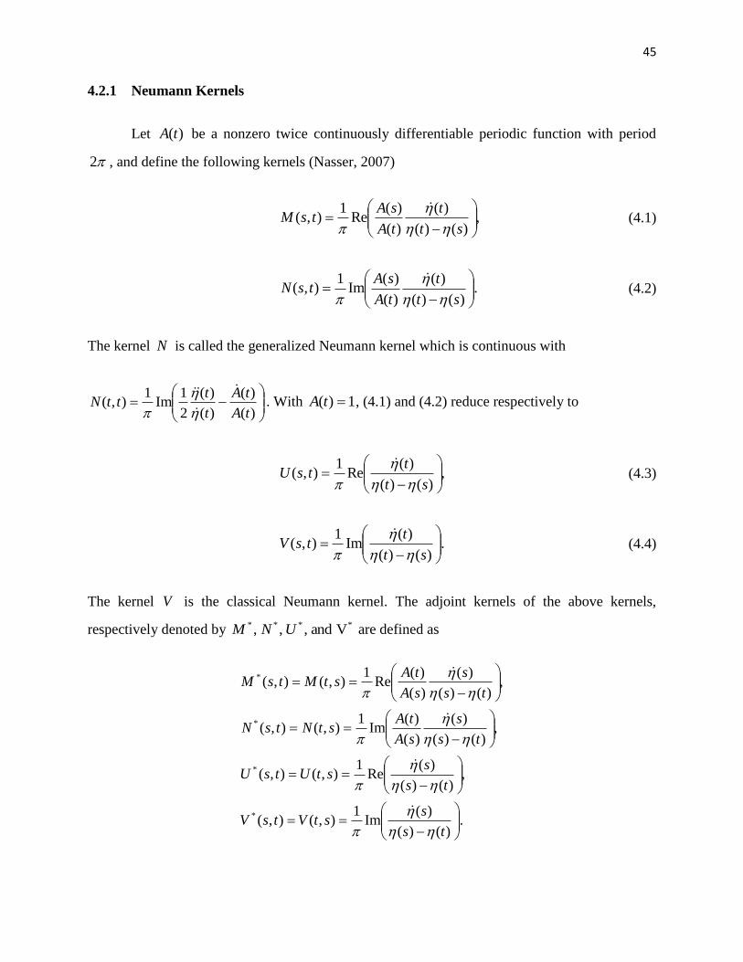
4.2.1 Neumann Kernels

Let )(tA be a nonzero twice continuously differentiable periodic function with period

2 , and define the following kernels (Nasser, 2007)

,)()(

)(

)(

)(Re

1),(

st

t

tA

sAtsM

(4.1)

.)()(

)(

)(

)(Im

1),(

st

t

tA

sAtsN

(4.2)

The kernel N is called the generalized Neumann kernel which is continuous with

)(

)(

)(

)(

2

1Im

1),(

tA

tA

t

tttN

. With 1)( tA , (4.1) and (4.2) reduce respectively to

,)()(

)(Re

1),(

st

ttsU

(4.3)

.)()(

)(Im

1),(

st

ttsV

(4.4)

The kernel V is the classical Neumann kernel. The adjoint kernels of the above kernels,

respectively denoted by **** Vand,,, UNM are defined as

.)()(

)(Im

1),(),(

,)()(

)(Re

1),(),(

,)()(

)(

)(

)(Im

1),(),(

,)()(

)(

)(

)(Re

1),(),(

*

*

*

*

ts

sstVtsV

ts

sstUtsU

ts

s

sA

tAstNtsN

ts

s

sA

tAstMtsM

46

4.2.2 The Neumann Problem

Consider the multiply connected region with smooth boundary. The Neumann

problem is to find a harmonic function ),( yxu defined on such that at each point of the

boundary , the directional derivative of u in the outward normal direction n is equal to a

function defined on this boundary. In other words, the solution u must satisfy the following

conditions

iyxzzu ,0)(2 , (4.5)

)(),(

))((tt

tu

n, (4.6)

where )(t is a known real continuous function defined on . The sufficient conditions for the

existences and uniqueness of the solution are given by

0)(,0)()(

udttt , (4.7)

where is a fixed point in .

The condition (4.7) is sometimes called the compatibility condition. Indeed, since u is harmonic

in , this implies that

.0)( 2

dzu

By using the divergence theorem, we get

0

dsu

n

which is just (4.7).

47

With the condition (4.7), a solution to (4.5) and (4.6) is guaranteed. However, the

solution is not unique. Indeed, by adding any constant to any particular solution u we still obtain

a solution. Therefore, the function u is required to satisfy the additional condition which can be

written as

,0)( u

where is a fixed point in .

4.2.3 The Riemann-Hilbert problem

Let be the multiply connected region as described before, and let )()()( tibtatA

be a non-zero complex function which is twice continuously differentiable periodic function with

period 2 , and let )(t and )(t be real Hölder continuously periodic functions with period

2 . The RH problem consists of finding a function ivug that is analytic in , continuous

in its closure and has boundary values ivug on which satisfy

),()()()()( ttvtbtuta

(4.8)

where in the superscript denotes the one-sided limit from the positive (or left) side of .

Equation (4.8) is called the Riemann condition which can also be written as

(4.9)

If we let )())](()(Im[ ttgtA , then the Riemann condition (4.9) is the real part of the

equation ).()())(()( tittgtA

Now, we define the adjoint RH problem as

)10.4(),())](()(~

Re[ ttgtA

). ( ))] ( ( ) ( Re[ t t g t A

48

where )(

)()(

~

tA

ttA

is the adjoint function of A .

The solvability of the RH problem depends on the index of the function A , which is denoted by

and it can be written as

)(arg2

1)(ind tAA

. We define the range space of the RH

problems and the solution space of the homogeneous RH problems as follows (Wegmann and

Nasser, 2008):

,inanalytic,~

:~

],~

Re[:~

,inanalytic,:],Re[:

ggAHSgAHR

gAgHSAgHR

where H is the space of real Hölder continuous functions on .

Theorem 4.1 (Wegmann and Nasser, 2008)

The solvability of the RH problem is connected with the solution space of the homogeneous

adjoint problem by the relations

,)(~

,)~

( SRSR

where denotes the orthogonal complement space.

Theorem 4.2 (Wegmann and Nasser, 2008)

The number of linearly independent solutions of the homogeneous RH problem and its adjoint

are connected by the formula

.21)~

dim()dim( mSS

49

4.2.4 Integral Equation for the RH Problem

There is a close relation between the RH problem and the integral equation with the

generalized Neumann kernel.

Theorem 4.3 (Wegmann and Nasser, 2008)

If g is a solution of the RH problem (4.9) with boundary values )()( titAg , then the

imaginary part satisfies the integral equation

MN , (4.11)

where the operators N and M are defined as

II

dtttsMsdtttsNs .)(),())((,)(),())(( MN

The solvability of this integral equation also depends on the index of the function A and

the connectivity of . This is clarified in the following theorem.

Theorem 4.4 (Wegmann and Nasser, 2008)

The number of linearly independent solutions of the homogeneous integral equations with

operator NI is given by

m

ii

m

ii

10

10

),12,0max()12,0max())(Nulldim(

),12,0max()12,0max())(Nulldim(

NI

NI

where I is the identity operator.

By this theorem and the Fredholm alternative theorem we can determine the solvability

of the integral equation (4.11).

50

4.3 A Boundary Integral Equation for the Neumann Problem

4.3.1 Reduction of the Neumann Problem to the RH Problem

Let )(zu be the solution of the Neumann problem on the multiply connected region .

Hence we can write u as a real part of an analytic function f defined on , i.e.

),()()( zivzuzf where v is the harmonic conjugate of u . Then the Neumann problem can

be reduced to the form (Alejaily, 2009)

).(|)(|))](')((Re[ ttift (4.12)

Equation (4.12) is the RH problem (4.9) with

).()()()),(('))((),()( ttttiftgttA

The method of reduction has also been used in Husin, (2009), but limited to the case of

interior Neumann problem on a simply connected region. With )()( ttA , the integral equation

(4.11) related to the RH problem (4.12) becomes

))(())(()( * sss uv* , (4.13)

where the operators *u and *

v are defined as

II

dtttsUsdtttsVs ,)(),())((,)(),())(( **** uv

and ),(),(* stUtsU and ),(),(* stVtsV are the adjoint kernels of U and V respectively.

51

4.3.2 Solvability of the RH Problem and the Derived Integral Equation

Since our RH problem (4.12) is the RH problem (4.9) with )()( ttA , the index for our

multiply connected region

m

jj

mt0

1))((ind . By applying Theorem 4.1 and Theorem

4.2 we get (Alejaily, 2009)

,)dim(,1)~

dim()codim(R mSS

where )codim(R represents the number of conditions for the right-hand side such that the RH

problem (4.9) is solvable. With regard to the integral equation (4.13), Theorem 4.4 implies that

m.))-Null(Null NIvI dim())(dim( *

This means that (4.13) is solvable subjected to m conditions on . So, we have non-uniquely

solvable RH problem (4.12) which gives rise to a non-uniquely solvable integral equation (4.13).

The value 1)codim(R means that the RH problem is solvable if and only if the right-hand

side satisfies a certain condition. This condition is the same as the solvability condition of

Neumann problem.

Now, we show how to obtain a unique solution of the integral equation (4.13), which will

give a unique solution of the RH problem (4.12). This means we have to impose m conditions

on the function to get a unique solution to the integral equation (4.13). Let us define the

kernel ),( tsJ for ji

IIts ),( such that (Atkinson, 1967)

.,,2,1,0,,,,,0

,,,2,1,,,2

1

),(

mjijiItIs

miItstsJ

ji

i

This means that ),( tsJ is equal to 1 when )(s and )(t belong to same boundary i except the

boundary 0 and equal to 0 otherwise. Then the integral operator J defined as

I

dtttsJs )(),())(( J satisfies (Alejaily, 2009)

52

kI

dtttsJs 0)(),())(( J . (4.14)

For mk ,,2,1 , this provides the m conditions for the function . By adding (4.14) to our

integral equation (4.13), we get

),)(())(())(()( ** ssss uJv (4.15)

which is uniquely solvable.

4.4 Numerical Implementation

We apply the Nyström method with the trapezoidal rule to discretize our integral

equation on an equidistant grid, where each interval ]2,0[ iI is subdivided into n steps of

size nh 2 . Since mi ,,1,0 , this leads to a system of nmr )1( equations in r

unknowns. Our choice of the trapezoidal rule was due to the periodicity of the functions A and

, where this method is very accurate for periodic functions (Davies and Rabinowitz, 1984). So,

the operators *v and *

u tend to be best described on an equidistant grid by the trapezoidal rule.

Then, we get the following linear system of equations

DCBI )( , (4.16)

where I is the identity matrix of dimension r while CB, and D are matrices of size rr ,

derived from the discretization of the operators Jv ,* and *

u respectively. and are 1r

vectors that approximate the values of functions and respectively at the collection points.

53

-6 -4 -2 0 2 4 6-4

-3

-2

-1

0

1

2

3

4

To solve the system (4.16), we have used the method of Gaussian elimination of

MATLAB. Since (4.15) is uniquely solvable, for n sufficiently large, the system of linear

equations (4.16) also has a unique solution (Atkinson, 1997).

4.5 Examples

In this section, we consider two examples of test regions to examine our method. The

sample problems are such that the analytic solutions are known. This allows us to compare our

numerical results with the exact solutions.

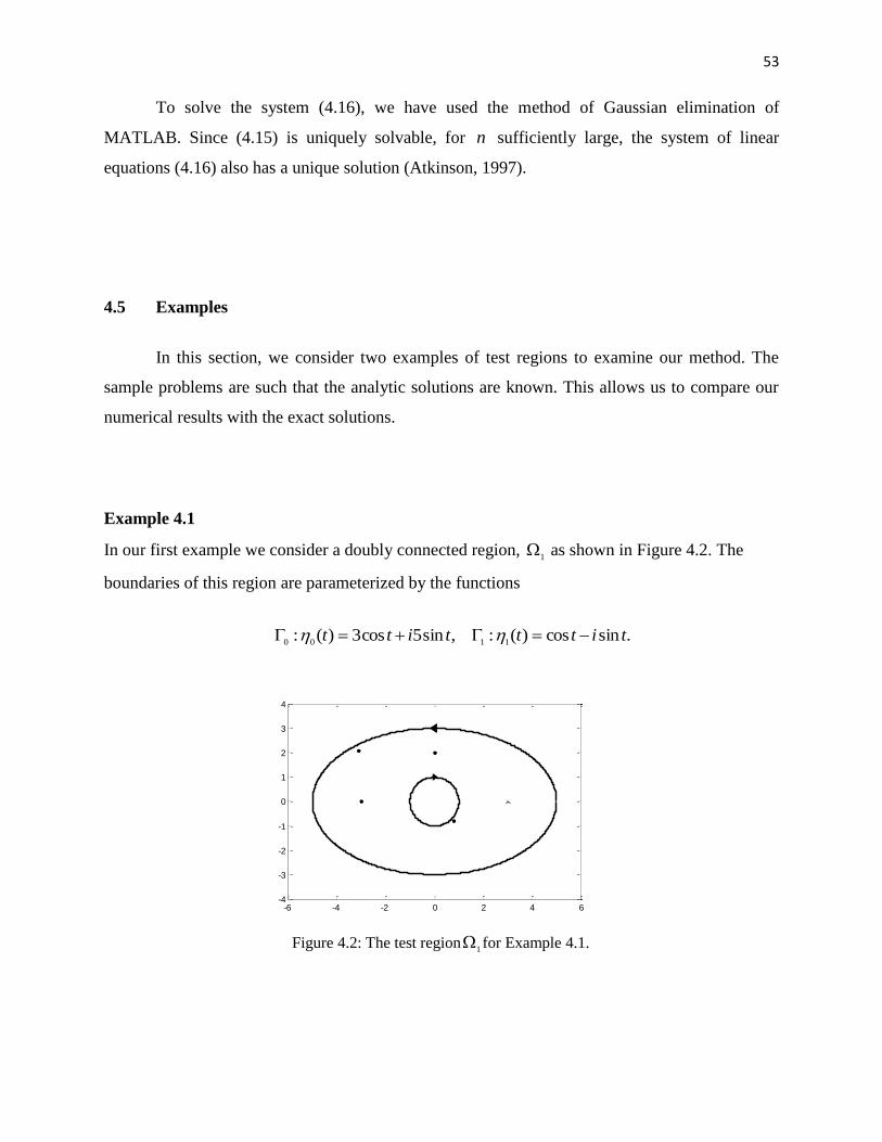
Example 4.1

In our first example we consider a doubly connected region, 1

as shown in Figure 4.2. The

boundaries of this region are parameterized by the functions

.sincos)(:,sin5cos3)(:1100

titttitt

Figure 4.2: The test region1

for Example 4.1.

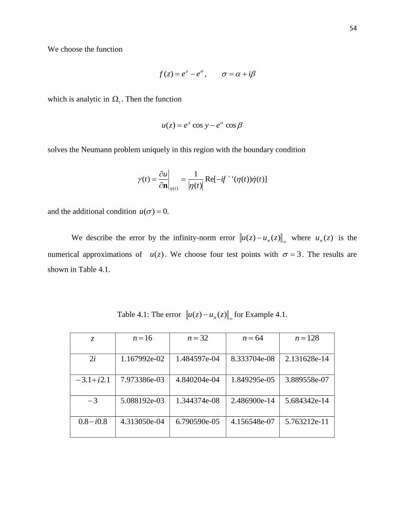
54

We choose the function

ieezf z ,)(

which is analytic in 1

. Then the function

coscos)( eyezu x

solves the Neumann problem uniquely in this region with the boundary condition

)]())(('Re[)(

1)(

)(

ttift

ut

t

n

and the additional condition .0)( u

We describe the error by the infinity-norm error

)()( zuzu n where )(zun is the

numerical approximations of )(zu . We choose four test points with 3 . The results are

shown in Table 4.1.

Table 4.1: The error

)()( zuzu n for Example 4.1.

z 16n 32n 64n 128n

i2 1.167992e-02 1.484597e-04 8.333704e-08 2.131628e-14

1.21.3 i 7.973386e-03 4.840204e-04 1.849295e-05 3.889558e-07

3 5.088192e-03 1.344374e-08 2.486900e-14 5.684342e-14

8.08.0 i 4.313050e-04 6.790590e-05 4.156548e-07 5.763212e-11

55

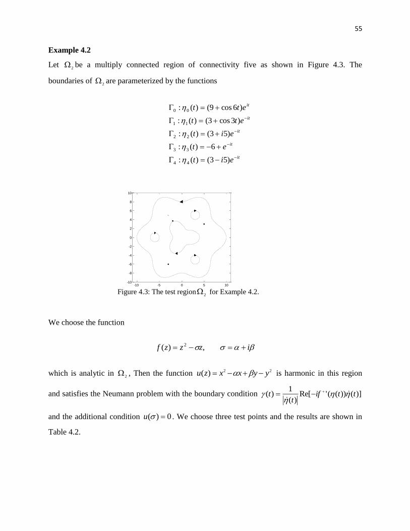
Example 4.2

Let 2

be a multiply connected region of connectivity five as shown in Figure 4.3. The

boundaries of 2

are parameterized by the functions

it

it

it

it

it

eit

et

eit

ett

ett

)53()(:

6)(:

)53()(:

)3cos3()(:

)6cos9()(:

44

33

22

11

00

We choose the function

izzzf ,)( 2

which is analytic in 2

, Then the function 22)( yyxxzu is harmonic in this region

and satisfies the Neumann problem with the boundary condition )]())(('Re[)(

1)( ttif

tt

and the additional condition 0)( u . We choose three test points and the results are shown in

Table 4.2.

-10 -5 0 5 10-10

-8

-6

-4

-2

0

2

4

6

8

10

Figure 4.3: The test region2

for Example 4.2.

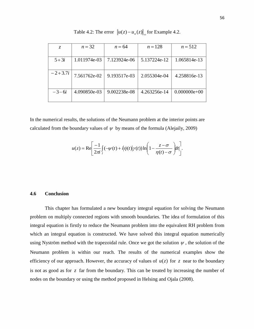
56

Table 4.2: The error

)()( zuzu n for Example 4.2.

z 32n 64n 128n 512n

i35 1.011974e-03 7.123924e-06 5.137224e-12 1.065814e-13

i7.32

7.561762e-02 9.193517e-03 2.055304e-04 4.258816e-13

i63 4.090850e-03 9.002238e-08 4.263256e-14 0.000000e+00

In the numerical results, the solutions of the Neumann problem at the interior points are

calculated from the boundary values of by means of the formula (Alejaily, 2009)

.)(

1ln))()()((2

1Re)(

dt

t

zttit

izu

I

4.6 Conclusion

This chapter has formulated a new boundary integral equation for solving the Neumann

problem on multiply connected regions with smooth boundaries. The idea of formulation of this

integral equation is firstly to reduce the Neumann problem into the equivalent RH problem from

which an integral equation is constructed. We have solved this integral equation numerically

using Nyström method with the trapezoidal rule. Once we got the solution , the solution of the

Neumann problem is within our reach. The results of the numerical examples show the

efficiency of our approach. However, the accuracy of values of )(zu for z near to the boundary

is not as good as for z far from the boundary. This can be treated by increasing the number of

nodes on the boundary or using the method proposed in Helsing and Ojala (2008).

57

CHAPTER 5

A BOUNDARY INTEGRAL EQUATION FOR THE EXTERIOR NEUMANN

PROBLEM ON MULTIPLY CONNECTED REGION

5.1 Introduction

Chapter 4 is on extended of Chapter 2 by formulating a new boundary integral equation

with Neumann kernel for solving the interior Neumann problem on multiply connected regions

with smooth boundaries. Chapter 4 has reduced the Neumann problem into the equivalent

Riemann-Hilbert problem from which an integral equation is constructed. The previous Chapter

3 has reduced the exterior Neumann problem on a simply connected region to exterior Riemann-

Hilbert problem by using Cauchy-Riemann equations. This leads to an integral equation with the

Neumann kernel. This chapter deals with the reduction of exterior Neumann problem on a

multiply connected region to the exterior Riemann-Hilbert problem. Thus this chapter extends

the results of Chapter 3.

This chapter is organized as follows: Section 5.2 presents some auxiliary materials

related to exterior Neumann and Riemann-Hilbert problems as well as integral equation for

Riemann-Hilbert problems. In Section 5.3, we reduce the exterior Neumann problem on multiply

connected region into the exterior Riemann-Hilbert problem and derive the boundary integral

58

Г3 Г2

2u = 0 T1

)(: 01 t

Г4 n

Ω¯

equation for solving it. Then, in Section 5.4, we provide a numerical technique for solving the

boundary integral equation by using Mathematica. Some numerical examples are presented in

Section 5.5. A short conclusion is given in Section 5.6.

5.2 Auxiliary Material

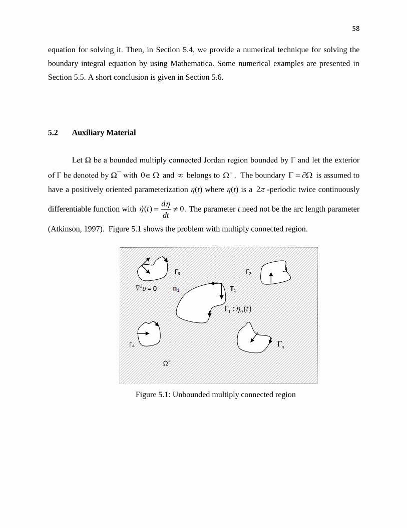
Let Ω be a bounded multiply connected Jordan region bounded by Г and let the exterior

of Г be denoted by Ω¯ with 0 and belongs to . The boundary is assumed to

have a positively oriented parameterization η(t) where η(t) is a 2 -periodic twice continuously

differentiable function with 0)( dt

dt

. The parameter t need not be the arc length parameter

(Atkinson, 1997). Figure 5.1 shows the problem with multiply connected region.

Figure 5.1: Unbounded multiply connected region

59

5.2.1 Boundary Integral Equation for Solving Exterior Neumann Problem

Denifition 5.1 (Atkinson,1997)

Let H represents a H lder space which consists all 2 -periodic real functions which are

uniformly Holder continuous with exponent . Let n be the exterior normal to Г and let H

be a given function such that

0)()(

2

0

dt . (5.1)

The exterior Neumann problem consists in finding the function u harmonic in Ω¯, H lder

continuous on Г and satisfies the boundary condition

.)(),()(

tt

u

t

n

(5.2)

The function u is also required to satisfy the additional condition

1)()( zOzu as z . (5.3)

Theorem 5.1 (Atkinson, 1997)

The exterior Neumann problem (5.2) is uniquely solvable.

According to Atkinson (1997), u satisfies an integral equation in the form of

)4.5(.,1

Log)(11

Log)(1

)(

dtt

tdttn

tuut

This equation is uniquely solvable and is considered a practical approach to solving the exterior

Neumann problem. The details regarding the numerical solution of the exterior Neumann

problem using this approach can be referred to Atkinson (1997).

60

Nasser (2007) has also developed a uniquely solvable second kind Fredholm integral

equation with the generalized Neumann kernel that can be used to solve the exterior Neumann

problems on simply connected regions with smooth boundaries. Suppose that u is the solution of

the exterior Neumann problem and v is a harmonic conjugate of u in Ω¯. Suppose ~~ i is a

boundary value of a function g analytic in Ω, i.e.,

)(~)(~))(( tittg , (5.5)

where

20)),(()(~)),(()(~ ttvttut

with )(~)( 1 zOczg near with a real constant c~ . Since

0)(Re)( zgzu when z

hence 0~ c . It is shown in Nasser (2007), that the boundary values of g can be written as

)).0(()( ivig (5.6)

where t

dttt0

)()()( and satisfies the integral equation

MN (5.7)

Since 0)( g then by Cauchy integral formula (Gakhov, 1966), the function )(zg for z

is in the form

d

z

tt

izg

)()(

2

1)( . (5.8)

Furthermore, the function g satisfies

0)(

2

1

d

g

i.

Hence, by (5.7),

d

i

iv

2

1))0(( . (5.9)

Then, the unique solution of the exterior Neumann problem is given in by

61

)(Re)( zgzu . (5.10)

The previous Chapter 3 has reduced the exterior Neumann problem on a simply

connected region to the equivalent exterior Riemann-Hilbert problem from which an integral

equation is constructed. The derived integral equation is in the form

BJV *, (5.11)

where 0)(2

1)(

2

0

dttJ and

.,)(

)(Im

2

1

,,)()(

)(Im

1

)(τ),(

tt

t

tt

VtN *

t,

The unique solution of the exterior Neumann problem on a simply connected region is given for

unbounded Ω in Chapter 3 as

)](Re[)( zfzu , (5.12)

where

2

0

)()(

1log)(

)()(

2

1)( dtt

z

t

ti

tit

izf

. (5.13)

The exterior Neumann problem has a unique solution u in Ω¯ which is not necessary

a real part of a single-valued analytic function f. However, there exist m real constants

,,,,21 m

aaa uniquely determined by , such that u can be written as the real part of

m

jjj zzazFzf

1

)log()()( , (5.14)

where F is a single-valued analytic function in Ω¯ (Mikhlin (1957), Muskhelishvili (1953)). The

real constants are chosen such that F is a single-valued analytic function in Ω¯, i.e.,

.,,2,1,0)(

j

mjdF (5.15)

62

It can be shown that

k

k dfi

a

)(2

1. Indeed, we have

1

)log()()(j

jj zzazfzF .

Differentiate the whole equation, we get

1

1)()(

j j

jzz

azfzF .

Then, integrate the equation we obtain

.1

)()(1

k kj

kj

j dz

adfdF

By the single-valuedness property,

.0)(

k

dF

Hence we get

,2)(0

k

kiadf

and finally we obtain

.)(2

1

df

ia

k

k

For Ω¯, the constants m

aaa ,,,21 satisfy

.0)(2

1)(

2

1

1 1

m

j

m

jj

j dfi

dfi

a

(5.16)

In view of (5.3), we can assume without loss the generality that 0)( f .

63

5.2.2 Boundary Integral Equation for Solving Exterior Riemann-Hilbert Problem

Suppose that Ω¯ is the exterior of Г such that the of the coordinate system belong to

Ω¯. If a function g(z) is defined in a region containing Г, then the limiting values of the function

g(z) when the point z tends to the point from the exterior of Г will be denoted by g¯(z).

Let A(t) be a complex continuously differentiable 2 -periodic function with 0A . With C,

H , let the function )(z be defined by

z

z

d

A

iC

iz ,

)(

)()(

2

1)(

. (5.17)

Then )(z is analytic in Ω as well as in Ω¯ and the boundary values from inside and

from outside belong to H and can be calculated by Plemelj‟s formula (see Atkinson (1967),

Asmar (2002))

,

)(

)()(

2

1PV

)(

)()(

2

1)(

z

d

A

iC

iA

iC. (5.18)

The integral (5.18) is a Cauchy principal value integral. The boundary values satisfy the jump

relation

iCAA . (5.19)

Definition 5.2 (Henrici (1986), Exterior Riemann-Hilbert Problem)

Given a function A and C, it is required to find a function g analytic in Ω¯ and continuous on the

closure with g( ) = 0 such that the boundary values g¯ satisfy

)(),())](()(Re[ ttCtgtA . (5.20)

The boundary condition (5.20) can be written in the equivalent form

)(,)(

)(2))((

)(

)()( t

tA

tCtg

tA

tAtg . (5.21)

64

The homogeneous boundary condition of the exterior Riemann-Hilbert problem is given by

)(,0))](()(Re[ ttgtA , (5.22)

where C(t) = 0.

The solvability of the Riemann-Hilbert problem is determined by the index κ of the

function A. The index of the function A is defined as winding number of A with respect to zero

(see Gakhov (1966), Murid and Nasser (2009)), i.e.,

2

0

)arg(2

1)(ind AA . (5.23)

We define the range space of the exterior Riemann-Hilbert problem, i.e., the space of

function C for which the exterior Riemann-Hilbert problem is solvable,

0)(,inanalytic))],(()(Re[)(: ggtgtAtCHCR . (5.24)

We defined the solution space of the homogenous exterior Riemann-Hilbert problem as

0)(,inanalytic)),(()()(: ggtgtAtCHCS . (5.25)

Then the number of arbitrary real constants in the solutions of the homogenous exterior

Riemann-Hilbert problems, i.e. dim ( S ) and the number of conditions on the function C so that

the non-homogenous exterior Riemann-Hilbert problems are solvable, i.e. codim( S ) are given

in term of the index κ as in the following theorem.

Theorem 5.2 [Gakhov (1966), Murid and Nasser (2009)]

The codimension of the space R and the dimension of the space S are given by the formulas

codim )( R = max(0, - 2κ + 1), (5.26)

dim )( S = max(0, 2κ – 1). (5.27)

Now, let A(t) be continuously differentiable 2 -periodic function with 0A . We define

two real functions N and M by

65

,)()(

)(

)(

)(Im

1),(

t

t

tA

AtN

(5.28)

.)()(

)(

)(

)(Re

1),(

t

t

tA

AtM

(5.29)

The kernel ),( tN is called the generalized Neumann kernel form with A and η (Wegmann et

al., 2005).

5.2.3 The Riemann-Hilbert Problem

We consider the same region as mentioned before and let A be a continuously

differentiable complex function on Г with A ≠ 0. We assume that A is given in parametric form

A(s) such that A(s) is continuously differentiable for all Js (Nasser, 2009). With H, ,

we define the function

z

z

d

A

i

iz ,

2

1)(

. (5.30)

Lemma 5.1 (Wegmann et al., 2005)

The boundary values of the function can be represented by

,))](()(Re[2 MN ssA (5.31)

.))](()(Im[2 NssA (5.32)

With assumptions about the lderoH continuity of the functions A, and , the

boundary functions is lderoH continuous on Г. The operators N and M map H into H

. Both operators are bounded in H .

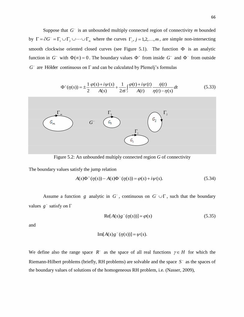
66

Suppose that G is an unbounded multiply connected region of connectivity m bounded

by m

G 21

where the curves mjj

,,2,1, , are simple non-intersecting

smooth clockwise oriented closed curves (see Figure 5.1). The function is an analytic

function in G with 0)( . The boundary values from inside G and from outside

G are lderoH continuous on Г and can be calculated by Plemelj‟s formulas

dtst

t

tA

tit

isA

siss

J )()(

)(

)(

)()(

2

1

)(

)()(

2

1))((

(5.33)

m

3

2

G

1

Figure 5.2: An unbounded multiply connected region G of connectivity

The boundary values satisfy the jump relation

).()())(()())(()( sisssAssA (5.34)

Assume a function g analytic in G , continuous on G , such that the boundary

values g satisfy on Г

)())](()(Re[ ssgsA (5.35)

and

).())](()(Im[ ssgsA

We define also the range space R as the space of all real functions H for which the

Riemann-Hilbert problems (briefly, RH problems) are solvable and the space S as the spaces of

the boundary values of solutions of the homogeneous RH problem, i.e. (Nasser, 2009),

67

,0)(,inanalytic],Re[: gGgAgHR (5.36)

.0)(,inanalytic,: gGgAgHS (5.37)

Theorem 5.3 (Nasser, 2009)

If g is a solution of the RH problem (5.35) with boundary values

)()( titAg (5.38)

then the imaginary part in (5.38) satisfies the integral equation

MN (5.39)

where the operators N and M are defined as

.)(),())((

,)(),())((

I

I

dtttsMs

dtttsNs

M

N

5.2.4 The Solvability of the Riemann-Hilbert Problem

The solvability on unbounded multiply connected regions can be deduced from the

solvability on bounded regions by means of Moebius transform (Wegmann, 2001). Let 0

z be a

fixed point in G , say m

Gz 0

. The unbounded region G is transformed by means of the

Moebius transform

0

1)(

zzz

(5.40)

onto a bounded multiply connected region )(ˆ GG of connectivity m. The Moebius

transform transforms also the bounded exterior region m

GGG 21

onto an unbounded

68

region G exterior to the boundary )(ˆˆ G . The boundary is given by

110ˆˆˆˆ

m where )(ˆ

0 m is the outer curve and is counterclockwise oriented;

and the other curves 1,,2,1),(ˆ mjjj

, are clockwise oriented and are inside 0 . The

curve is parameterized by (Nasser, 2009)

.,)(

1)(

0

Jszs

s

(5.41)

Let the function A be defined by

.),()()(ˆ JssAssA (5.42)

According Nasser (2009), for a given H , a function g analytic in G with

0)(ˆ g , continuous on ˆG , such that the boundary values g satisfy on

).())]((ˆ)(ˆRe[ ssgsA (5.43)

We define also the spaces

,Ginanalyticˆ],ˆˆRe[:ˆ -ggAHR (5.44)

.ˆinanalyticˆ,ˆˆ:ˆ GggAHS (5.45)

Lemma 5.2 (Nasser, 2009)

The spaces SRSR ˆandˆ,, satisfy

.ˆ,ˆ SSRR (5.46)

The index of the function A on the whole boundary curve Г is the sum

,1

m

jj (5.47)

where the j

of the function A on the curve j

is defined as the winding number of A with

respect to 0, i.e.

.,,2,1,)(arg2

1mjA

jj

(5.48)

69

Theorem 5.4 (Wegmann and Nasser, 2008)

The dimension of the space S and the codimension of the space R are determined by the index

of A as follows:

a) If ,0 then

.2)dim(co,0)dim( mRS (5.49)

b) If m , then

.0)dim(co,2)dim( RmS (5.50)

c) If 11 m , then

.)dim(2,)dim(2 mRcomSm (5.51)

Theorem 5.5 (Wegmann and Nasser, 2008)

The dimensions of the null-spaces of the operators NI are given by

,)12,0max())(Nulldim(1

m

jj

I N (5.52)

.)12,0max())(dim(1

m

jjINull N (5.53)

5.3 Modification of the Exterior Neumann Problem

5.3.1 Reduction of the Exterior Neumann Problem to the Exterior Riemann-Hilbert

Problem

Let )(zu be the solution of the exterior Neumann problem on the multiply connected

region . Hence we can write u as a real part of an analytic function f defined on

, i.e.

),()()( zivzuzf

70

where v is the harmonic conjugate of u. The derivative of f with respect to z is given by

),()()( zivzuzf xx

where x

uu x

and

y

uu y

.

The boundary values of f and f are

).()()('

),()()(

xx ivuf

ivuf

The normal derivative of f is given by

.)()()(

nnn

vi

uf (5.54)

From vector calculus, we can write

njin

njin

)(

,)(

yx

yx

uvv

uuu

If

,jin yx nn

where yx nn , are the components of the outward vector, then (5.54) becomes

).()()()()(

jijijijin

yxyxyxyx nnvvinnuuf

After some arrangement, we get

).(')()(

f

vi

un

nn

Equating real parts on both sides we get

71

)(')(

)(Re)(

)(

f

t

tit

u

n

which is equivalent to

).()())](')((Re[ ttift (5.55)

Equation (5.55) is the RH problem (5.35) with

).()()()),(('))((),()( ttttiftgttA (5.56)

The above method of reduction is only limited to the case of exterior Neumann problem on a

simply connected region.

5.3.2 Integral Equation Related to the Exterior Riemann-Hilbert Problem

In this section, we will show the way to construct an integral equation related to the RH

problem (5.55) based on Theorem 5.3. With )()( ttA , then

),,()()(

)(Re

1

)()(

)(

)(

)(Re

1),(

),,()()(

)(Im

1

)()(

)(

)(

)(Im

1),(

tsUts

s

st

t

t

stsM

tsVts

s

st

t

t

stsN

*

*

where *U and *V are the adjoint kernels of U and V respectively. Then the integral equation

(5.39) related to the RH problem (5.55) becomes

**uv (5.57)

where the operators *u and *

v are defined as

72

I

I

dtttsUs

dtttsVs

.)(),())((

,)(),())((

*

*

*

*

u

v

5.3.3 The Solvability of the Exterior Riemann-Hilbert Problem

Since our RH problem (5.55) is the RH problem (5.35) with )()( ttA , the index

))((ind t for exterior multiply connected region Ω implies

.,,3,2,1,1 mjj

Hence, we have

.1

m

jj m

For the doubly connected regions, we have 2m and

.1,1 21

Hence,

.221

From Theorem 3.2, we obtain

,0)codim( R (5.58)

.2)dim( S (5.59)

Equation (5.58) means that there is no condition for in (5.55), so that the non-homogeneous

exterior Riemann-Hilbert problem is solvable. Equation (5.59) implies that, there are two real

constants in the solution of the homogeneous exterior Riemann-Hilbert problem so that the

solution of the exterior Riemann-Hilbert problem is not unique.

73

To overcome the non-uniqueness, we need to impose additional constraint which can be

embedded into integral equation that will yield a uniquely solvable integral equation.

5.3.4 Modified Integral Equation for the Exterior Riemann-Hilbert Problem

Recall from Chapter 3 Section 3.2.3 with ( ) ( )A t t , the generalized Neumann kernel N

becomes

stt

t

stts

s

tsN

,)(

)(Im

2

1

,)()(

)(Im

1

),(

(5.60)

= ),,(* tsV (5.61)

while the kernel M becomes

)()(

)(Re

1),(

ts

stsM

(5.62)

= ).,(* tsU (5.63)

So, our non-uniquely solvable integral equation (5.39) becomes (5.57) and can be rewritten in

the form below,

II

I I

dttts

sdtt

ts

ss

dtttsMdtttsNs

tts

,)()()(

)(Re

1)(

)()(

)(Im

1)(

,)(),()(),()(

),()()(

MN

74

.)()()(

)(Re

1)(

)()(

)(Im

1)(

II

dttts

sdtt

ts

ss

(5.64)

For 1

Is , equation (5.64) becomes

2

0

2

0

2

21

11

11

11 )(

)()(

)(Im

1)(

)()(

)(Im

1)( t

ts

sdtt

ts

ss

2

0

2

0

2

21

11

11

1 .)()()(

)(Re

1)(

)()(

)(Re

1dtt

ts

sdtt

ts

s (5.65)

For 2

Is , equation (5.64) becomes

2

0

2

0

2

22

21

12

22 )(

)()(

)(Im

1)(

)()(

)(Im

1)( t

ts

sdtt

ts

ss

.)()()(

)(Re)(

)()(

)(Re

1 2

0

2

22

22

0

1

12

2

dtt

ts

sdtt

ts

s (5.66)

Recall from Section 5.3.1, that the function f is analytic on . Then at each point z

in that domain when )(,00

zfz can be represented by the following Laurent series expansion

such that 0)( f :

3

3

2

21)(z

c

z

c

z

czf (5.67)

Differentiate once with respect to z and multiply with –iz we will obtain

)(32

)(3

3

2

21 zFz

c

z

c

z

czfzi (5.68)

Since )),(('))(( tiftg

.)(

)(z

zFzg

(5.69)

By means of Cauchy-Formula and the fact from Gakhov (1966, p.24),

75

,0)()(

2

1

FdF

i

(5.70)

,0)(2

1

dgi

(5.71)

.0)(

dg (5.72)

From (5.38), )(

)()())((

t

tittg

where )()( ttA , so (5.72) becomes

,0)()(

)()(

dttt

tit

(5.73)

.0)()(2

0

2

0

dttidtt (5.74)

Note that, the exterior Neumann problem need to satisfy (4.7) in Chapter 4. From (5.55),

).()()( ttt

Therefore, (4.7) becomes

.0)(2

0

dtt (5.75)

We consider (5.75) as the additional condition for the exterior Riemann-Hilbert problem which

the right-hand side of the Riemann-Hilbert problem (5.55) need to satisfy. Thus from (5.75),

(5.74) becomes

.0)(2

0

dtt (5.76)

Let us define the kernel ),( tsJ for ji IIts ),( such that

.,,2,1,,,,,0

,,2,1,,,2

1

),(

mjijiItIs

miItstsJ

ji

i

This means that ),( tsJ is equal to 1 when )(),( ts belong to same boundary i and equal to 0

otherwise. Then we define the operator J by

.)(),())(( I

dtttsJs J (5.77)

76

Adding (5.77) into (5.57) yields the new integral equation

**uJv (5.78)

which is uniquely solvable.

5.3.5 Modifying the Singular Integral Operator

Consider the right-hand side of (5.78),

.)()()(

)(Re

1)(),(*

II

dttts

sdtttsU

*u (5.79)

Using the fact that

,0)()(

)(Re

1

I

dtst

t

(5.80)

(5.79) becomes

,),(

)()(

)(

)(

)(

)(

)()(Re1

)()(

)(Re

1)()(

)()(

)(Re

1

)()(

)(Re

1)()(

)()(

)(Re

1

)()(

)(Re

1)()(

)()(

)(Re

1)(),(*

I

I

I I

I I

III

dttsB

dtst

s

s

t

t

ts

dtst

tsdtt

st

s

dtst

tsdtt

st

s

dtst

tsdtt

ts

sdtttsU

where

77

1 ( ) ( ) ( ) ( )( , ) Re

( ) ( )

s t t sB s t

t s

, (5.81)

for s t . We now show that ( , )B s t also exists for s t .

Letting

and

2

, so that

,)()(

)()()()(Re

1),(

st

sttstsB

and

.)(

)(

)()(

)()(lim

t

t

st

st

ts

Thus, the values of ),( tsB on the diagonal are

)(

)(

)()()()(

)()(Re1

),(2

t

t

tttt

ttttB

.)(

)(Re)()(

1

t

ttt

(5.82)

Then, we define the integral operator with kernel B as

I

dttsB ),(B (5.83)

So, the uniquely solvable integral equation (5.78) become

BJv* (5.84)

and it has the integral form

I II

dttsBdtttsJdtttsVs .),()(),()(),()( * (5.85)

78

5.3.6 Computing and

After solving for from the integral equation (5.84), the boundary values of the function

f are computed from (5.38) and (5.55), i.e.,

).()())((')( tittfti (5.86)

In view of (5.86), the Cauchy integral formula implies that the function )(zf can be calculated

for z by

II

dtzt

t

ti

tit

id

z

f

izf

)(

)(

)(

)()(

2

1)(

2

1)('

.)(

)(

)(

)()(

2

1

)(

)(

)(

)()(

2

1 2

0 2

2

2

222

0 1

1

1

11

dt

zt

t

ti

tit

idt

zt

t

ti

tit

i

(5.87)

i.e., the function )(' zf is represented by a Cauchy type integral. To calculate the values of f,

we apply the formula of the integral representation of an analytic function the mth derivative of

which is representable by the Cauchy type integral (Gakhov, 1966). The kernel of this formula

depends on the integration of the Cauchy kernel. In our case, the formula is

I

dttz

tf

izf )(

)(1log)('

2

1)(

.)()(

1log)('2

1)(

)(1log)('

2

1 2

0

2

0

22

2211

11

dttz

tf

idtt

z

tf

i (5.88)

Hence, the unique solution of the Neumann problem, u, can be evaluated from

)].(Re[)( zfzu (5.89)

79

5.4 Numerical Implementations of the Boundary Integral Equation

Since the function )(tA and )(t are 2 -periodic, the integrals in the integral equation

(5.85) can be best discretized on an equidistant grid by the trapezoidal rule, i.e., the integral

operators are discretized by the Nyström method with the trapezoidal rule as the quadrature rule.

Let n be a given integer and define the n equidistant collocation points j

t by

.,,2,1,2

)1( njn

jt j

(5.90)

Then, using the Nyström method with the trapezoidal rule to discretized the integral equation

(5.85), we obtain the linear systems

.),(2

)(),(2

)(),(2

)(111

n

jij

n

jjnjijnji

n

j

*

in ttBn

tttJn

tttVn

t

(5.91)

with ni ,,2,1 and n is an approximation to .

Let I be the nn matrix. Also let 11I and 22I be the nn matrix and 1I be the 1n

vector whose elements are all unity. Defining the matrix ][],[],[ jijiji BBJJVV and vector

][],[ jj yyx x by

ji

i

i

ji

kj

j

ji

*

ji

ttt

t

tttt

t

nttV

n,

)(

)(Im

2

1

,)()(

)(Im

1

2),(

2

V (5.92)

22112

12

2

12),(

2II

nnttJ

njijiJ (5.93)

80

kj

j

j

jj

kj

ij

ijji

ijji

ttt

ttt

tttt

tttt

n

ttBn

,)(

)(Re)()(

1

,)()(

)()()()(Re

1

2

),(2

B

(5.94)

)( jnj tx (5.95)

and

1Ijij By . (5.96)

Hence, the application of Nyström method to the uniquely solvable integral equation

(5.85) leads to the following n by n linear system

.)( yxJVI (5.97)

By solving the linear system (5.97) using Gaussian elimination, we obtain )( jn t for

nj ,,2,1 Then the approximate solution )(tn can be calculated for all ]2,0[ t using the

Nyström interpolating formula, i.e., the approximation )(tn of the integral equation (5.83) is

given by

.)(),(2

)(),(2

),(2

)(11

*

1

n

iiniini

n

i

n

iin tttJ

ntttV

nttB

nt

(5.98)

By obtaining , (5.87) and (5.88) implies that the function )(' zf and )(zf can be calculated

for z .

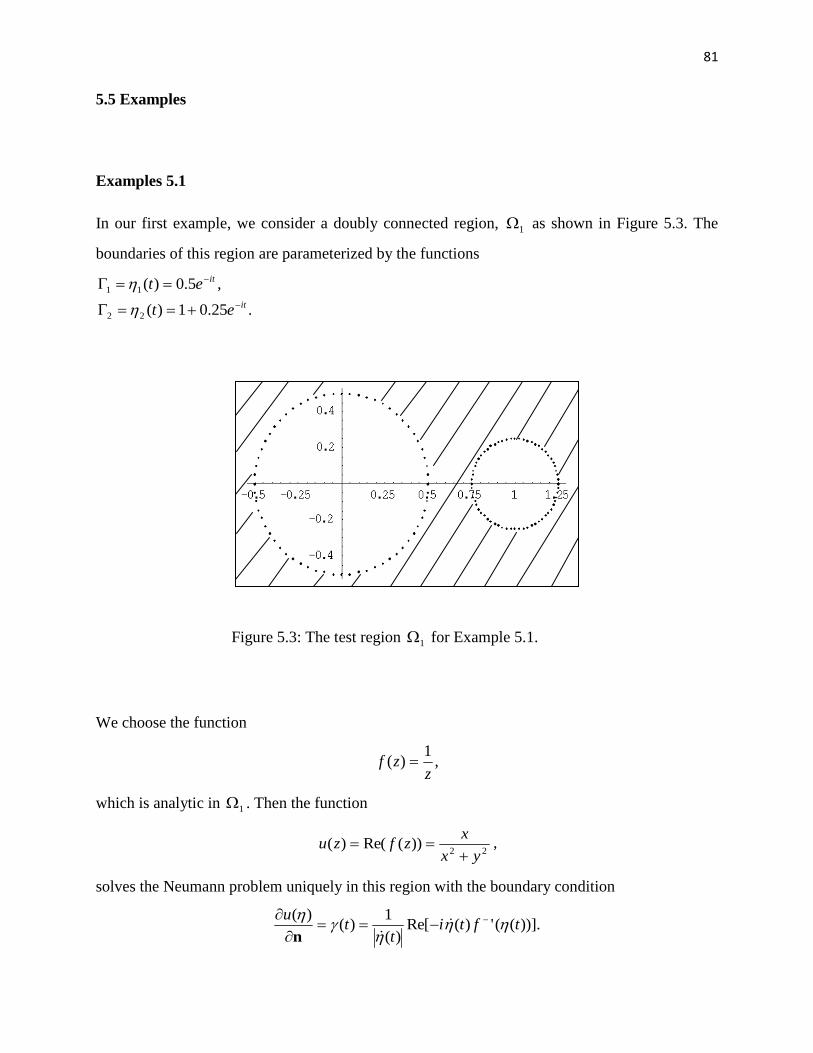
81

5.5 Examples

Examples 5.1

In our first example, we consider a doubly connected region, 1 as shown in Figure 5.3. The

boundaries of this region are parameterized by the functions

.25.01)(

,5.0)(

22

11

it

it

et

et

Figure 5.3: The test region 1 for Example 5.1.

We choose the function

,1

)(z

zf

which is analytic in 1 . Then the function

22))(Re()(

yx

xzfzu

,

solves the Neumann problem uniquely in this region with the boundary condition

))].((')(Re[)(

1)(

)(tfti

tt

u

n

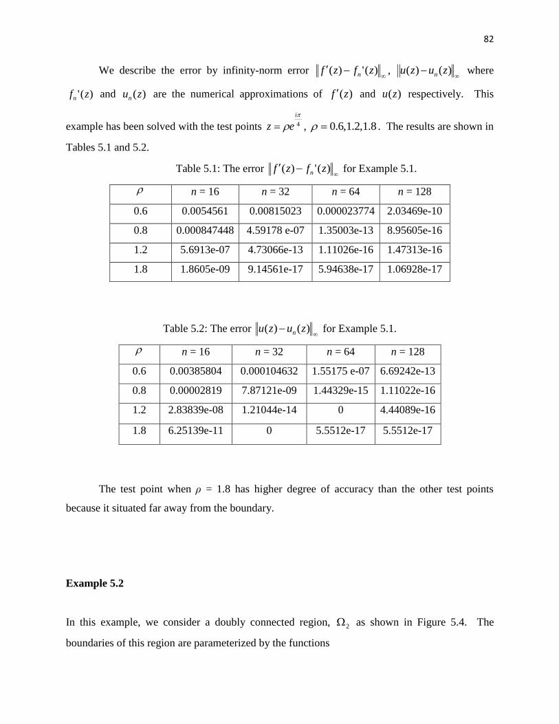
82

We describe the error by infinity-norm error

)(')( zfzf n ,

)()( zuzu n where

)(' zfn and )(zun are the numerical approximations of )(zf and )(zu respectively. This

example has been solved with the test points 4

i

ez , 8.1,2.1,6.0 . The results are shown in

Tables 5.1 and 5.2.

Table 5.1: The error

)(')( zfzf n for Example 5.1.

n = 16 n = 32 n = 64 n = 128

0.6 0.0054561 0.00815023 0.000023774 2.03469e-10

0.8 0.000847448 4.59178 e-07 1.35003e-13 8.95605e-16

1.2 5.6913e-07 4.73066e-13 1.11026e-16 1.47313e-16

1.8 1.8605e-09 9.14561e-17 5.94638e-17 1.06928e-17

Table 5.2: The error

)()( zuzu n for Example 5.1.

n = 16 n = 32 n = 64 n = 128

0.6 0.00385804 0.000104632 1.55175 e-07 6.69242e-13

0.8 0.00002819 7.87121e-09 1.44329e-15 1.11022e-16

1.2 2.83839e-08 1.21044e-14 0 4.44089e-16

1.8 6.25139e-11 0 5.5512e-17 5.5512e-17

The test point when ρ = 1.8 has higher degree of accuracy than the other test points

because it situated far away from the boundary.

Example 5.2

In this example, we consider a doubly connected region, 2 as shown in Figure 5.4. The

boundaries of this region are parameterized by the functions

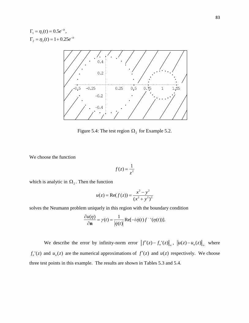
83

it

it

et

et

25.01)(

,5.0)(

22

11

Figure 5.4: The test region 2 for Example 5.2.

We choose the function

2

1)(

zzf

which is analytic in 2 . Then the function

222

22

)())(Re()(

yx

yxzfzu

solves the Neumann problem uniquely in this region with the boundary condition

))].((')(Re[)(

1)(

)(tfti

tt

u

n

We describe the error by infinity-norm error

)(')( zfzf n ,

)()( zuzu n where

)(' zfn and )(zun are the numerical approximations of )(zf and )(zu respectively. We choose

three test points in this example. The results are shown in Tables 5.3 and 5.4.

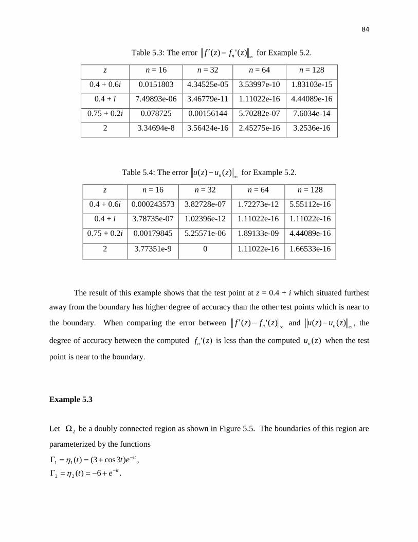
84

Table 5.3: The error

)(')( zfzf n for Example 5.2.

z n = 16 n = 32 n = 64 n = 128

0.4 + 0.6i 0.0151803 4.34525e-05 3.53997e-10 1.83103e-15

0.4 + i 7.49893e-06 3.46779e-11 1.11022e-16 4.44089e-16

0.75 + 0.2i 0.078725 0.00156144 5.70282e-07 7.6034e-14

2 3.34694e-8 3.56424e-16 2.45275e-16 3.2536e-16

Table 5.4: The error

)()( zuzu n for Example 5.2.

z n = 16 n = 32 n = 64 n = 128

0.4 + 0.6i 0.000243573 3.82728e-07 1.72273e-12 5.55112e-16

0.4 + i 3.78735e-07 1.02396e-12 1.11022e-16 1.11022e-16

0.75 + 0.2i 0.00179845 5.25571e-06 1.89133e-09 4.44089e-16

2 3.77351e-9 0 1.11022e-16 1.66533e-16

The result of this example shows that the test point at z = 0.4 + i which situated furthest

away from the boundary has higher degree of accuracy than the other test points which is near to

the boundary. When comparing the error between

)(')( zfzf n and

)()( zuzu n , the

degree of accuracy between the computed )(' zfn is less than the computed )(zun when the test

point is near to the boundary.

Example 5.3

Let 2 be a doubly connected region as shown in Figure 5.5. The boundaries of this region are

parameterized by the functions

.6)(

,)3cos3()(

22

11

it

it

et

ett

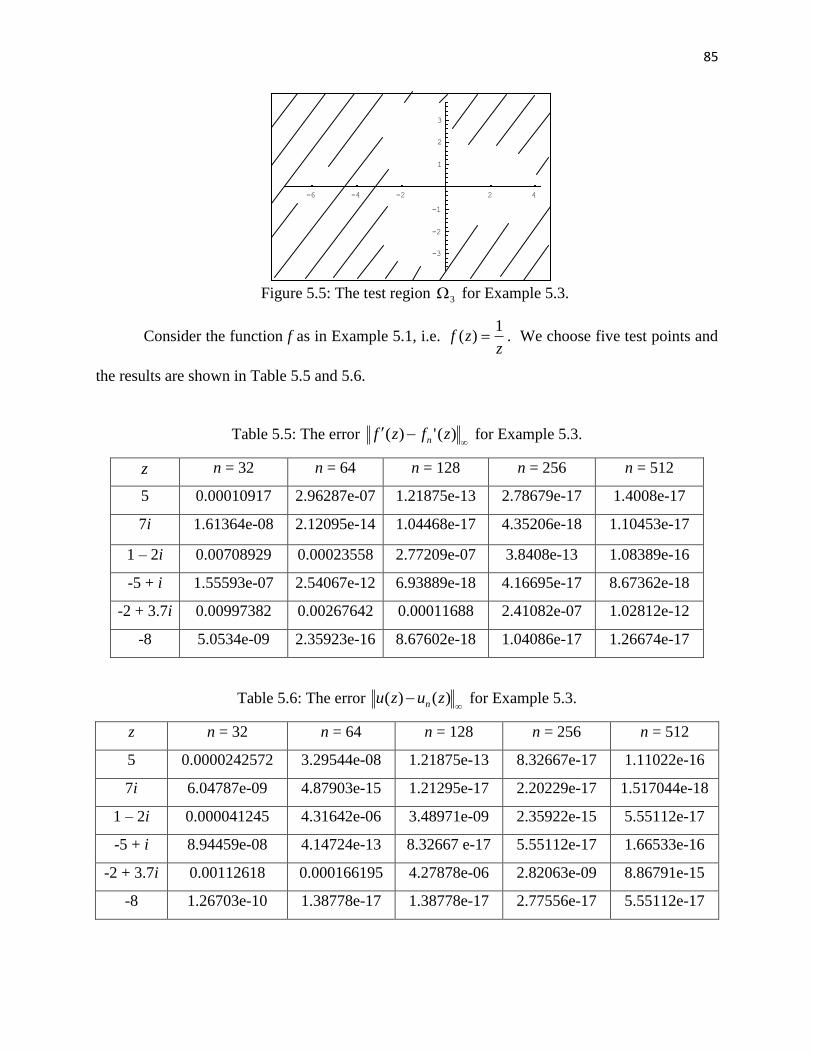
85

Figure 5.5: The test region 3 for Example 5.3.

Consider the function f as in Example 5.1, i.e. z

zf1

)( . We choose five test points and

the results are shown in Table 5.5 and 5.6.

Table 5.5: The error

)(')( zfzf n for Example 5.3.

z n = 32 n = 64 n = 128 n = 256 n = 512

5 0.00010917 2.96287e-07 1.21875e-13 2.78679e-17 1.4008e-17

7i 1.61364e-08 2.12095e-14 1.04468e-17 4.35206e-18 1.10453e-17

1 – 2i 0.00708929 0.00023558 2.77209e-07 3.8408e-13 1.08389e-16

-5 + i 1.55593e-07 2.54067e-12 6.93889e-18 4.16695e-17 8.67362e-18

-2 + 3.7i 0.00997382 0.00267642 0.00011688 2.41082e-07 1.02812e-12

-8 5.0534e-09 2.35923e-16 8.67602e-18 1.04086e-17 1.26674e-17

Table 5.6: The error

)()( zuzu n for Example 5.3.

z n = 32 n = 64 n = 128 n = 256 n = 512

5 0.0000242572 3.29544e-08 1.21875e-13 8.32667e-17 1.11022e-16

7i 6.04787e-09 4.87903e-15 1.21295e-17 2.20229e-17 1.517044e-18

1 – 2i 0.000041245 4.31642e-06 3.48971e-09 2.35922e-15 5.55112e-17

-5 + i 8.94459e-08 4.14724e-13 8.32667 e-17 5.55112e-17 1.66533e-16

-2 + 3.7i 0.00112618 0.000166195 4.27878e-06 2.82063e-09 8.86791e-15

-8 1.26703e-10 1.38778e-17 1.38778e-17 2.77556e-17 5.55112e-17

-6 -4 -2 2 4

-3

-2

-1

1

2

3

86

From the results above, when the test points are near to the boundary, we get less degree

of accuracy, and the degree of accuracy of the computed )(' zfn

is less than the computed )(zun

.

5.6 Conclusion

The reduction of the exterior Neumann problem on multiply connected region into the

exterior Riemann-Hilbert problem is derived which leads to a non-uniquely solvable boundary

integral equation. Additional constraint to the solution of the problem is required so that the

problem is uniquely solvable. The related integral equation is modified to obtain uniquely

solvable integral equation. Furthermore, we also presented the numerical implementations of the

derived boundary integral equation in this chapter. The integral equation was solved by Nyström

method with the trapezoidal rule as the quadrature rule. The exterior multiply connected

Neumann problems were then solved numerically in three test regions using the proposed

method. The numerical examples illustrated that the proposed method yields approximation of

high accuracy.

87

CHAPTER 6

CONCLUSIONS AND SUGGESTIONS

6.1 Conclusions

A Neumann problem is a boundary value problem of determining a harmonic function

( , )u x y interior or exterior to a region with prescribed values of its normal derivative /du dn on

the boundary. This research has presented several new boundary integral equations for the

solution of Laplace‟s equation on both bounded and unbounded multiply connected regions, with

the Neumann boundary condition. The method is based on uniquely solvable Fredholm integral

equations of the second kind with the generalized Neumann kernel. The idea of formulation of

these integral equations is firstly to reduce the Neumann problem on each region into the

equivalent RH problem from which an integral equation is constructed. We have solved these

integral equations numerically using Nyström method with the trapezoidal rule. Once we got the

solutions of the integral equations, the solutions of the Neumann problems are within our reach.

Several results of the numerical examples show the efficiency of our approach.

88

6.1.1 Name of articles/ manuscripts/ books published

M.M.S. Nasser, A.H.M. Murid, M. Ismail, E. M. A. Alejaily, Boundary Integral

Equations with the Generalized Neumann Kernel for Laplace‟s Equation in

Multiply Connected Regions, Journal in Applied Mathematics and Computation,

Vol. 217 (Jan 2011), 4710 – 4727. (IF: 1.125)

E.M.A. Alejaily, Azlina Jumadi, Ali H.M. Murid, Hamisan Rahmat, “Computing

the Solution of the Neumann Problem Using Integral Equation and Runge-Kutta

Method”, Proceedings of the Regional Annual Fundamental Science Symposium

(RAFSS 2010), Ibnu Sina Institute, UTM, 51 – 61.

Laey-Nee Hu, Ali H.M. Murid and Mohd Nor Mohamad, An Integral Equation

Method for Conformal Mapping of Multiply Connected Regions onto an Annulus

with Circular Slits via the Neumann Kernel, CD Proceedings of the 5th Asian

Mathematical Conference (AMC) 2009.

Eijaily M.A. Alejaily, Ali H.M. Murid & Mohamed M.S. Nasser, A Boundary

Integral Equation for the Neumann Problem in Bounded Multiply Connected

Region, Proceedings of the Simposium Kebangsaan Sains Matematik ke-17 (2009),

201-207.

Azlina Jumadi, Munira Ismail & Ali H.M. Murid, An Integral Equation method for

solving Exterior Neumann Problems on Smooth Regions, Proceedings of the

Simposium Kebangsaan Sains Matematik ke-17 (2009), 208-215.

Ejaily Milad Ahmed Alejaily, A Boundary Integral Equation for the Neumann

Problem in Bounded Multiply Connected Region, M.Sc. Dissertation (2009) UTM.

Azlina Jumadi, An Integral Equation Method for Solving Exterior Neumann

Problems on Smooth Regions, M.Sc. Dissertation (2009) UTM.

Chye Mei Sian, A Boundary Integral Equation for the Exterior Neumann Problem

on Multiply Connected Region, M.Sc. Dissertation (2010) UTM.

89

6.1.2 Title of Paper Presentations (international/ local)

International Conference on Computational and Function Theory, 8-12 June 2009,

Bilkent University, Ankara, Turkey. Title of paper: A Boundary Integral Equation

with the Generalized Neumann Kernel for Laplace‟s Equation in Multiply

Connected Regions. Authors: Mohamed M.S. Nasser and Ali H.M. Murid

(presenter).

5th

Asian Mathematical Conference (AMC 2009), 22-26 Jun 2009, PWTC Kuala

Lumpur. Title of paper: A Boundary Integral Equation for Conformal Mapping of

Multiply Connected Regions onto the Circular Slit Regions Via The Neumann

Kernel. Authors: Laey-Nee Hu (presenter), Ali H.M. Murid and Mohd Nor

Mohamad.

2nd

International Conference and Workshops on Basic and Applied Sciences and

Regional Annual Fundamental Science Seminar (ICORAFFS 2009), 3-4 June 2009,

The Zone Regency Hotel, Johor Bahru. Title of paper: An Integral Equation

Method for Solving Neumann Problems in Simply Connected Regions with Smooth

Boundaries. Authors: Ali H.M. Murid, Ummu Tasnim Husin (Presenter) and

Hamisan Rahmat.

Regional Annual Fundamental Science Symposium 2010 (RAFSS2010), 8-9 June

2010, Grand Seasons Hotel, Kuala Lumpur. Title: Computing the Solution of the

Neumann Problem Using Integral Equation and Runge-Kutta Method. Authors: E.

M. A. Alejaily, Azlina Jumadi, Ali H. M. Murid (presenter) and Hamisan Rahmat.

Simposium Kebangsaan Sains Matematik Ke-17, 15-17 Dis 2009, Hotel Mahkota

Melaka; Title of paper: A Boundary Integral Equation for the Neumann Problem in

Bounded Multiply Connected Region,Penulis: E. M. A. Alejaily, A. H. M. Murid

(presenter) and M.M.S. Nasser.

Simposium Kebangsaan Sains Matematik Ke-17, 15-17 Dis 2009, Hotel Mahkota

Melaka; Title of paper: An Integral Equation method for solving Exterior Neumann

Problems on Smooth Regions,Penulis: Azlina Jumadi (presenter), Munira Ismail &

Ali H.M. Murid.

90

6.1.3 Human Capital Development

Four M.Sc. students (completed)

One Research Officer

6.2 Suggestions for Future Research

This research develops a method to solve the Neumann problem within certain conditions

and assumptions. For further research, we suggest the following

We mentioned in the previous chapter that we lost some accuracy of values of as we

get closer to the boundaries. This lost, we think, can be reduced if we study the

possibility of improving the formula (5.89) along the same lines as we have done for

evaluating .

In this research we did not calculate the solution of the Neumann problem on the

boundaries . This can be achieved if we calculate from . For that we

suggest to treat the formula (5.86) as a differential equation and apply, for example, the

Runge-Kutta method to solve it.

The domains of the problems in this research are multiply connected regions with smooth

boundaries. We propose extending our approach for multiply connected regions with

nonsmooth boundaries.

The general theories were developed for solving the interior and exterior Neumann

problems on multiply connected region. Other potential applications need to be explored.

Probably some extensions or modifications of the theories are required to obtain integral

equations related to mixed boundary value problem with Dirichlet-Neumann boundary

conditions.

91

REFERENCES

E.M.A. Alejaily, A Boundary Integral Equation for the Neumann Problem in Multiply

Connected Region, M.Sc. Dissertation, UTM, 2009.

F. K. Anh, Two Approximate Methods for solving Nonlinear Neumann Problems, Ukrainian

Mathematical Journal, 40 (1988), 527-532.

K. E. Atkinson, The Numerical Solution of Integral Equations of the Second Kind, Cambridge

University Press, 1997.

K. E. Atkinson, The solution of non-unique linear integral equations, Numerische Mathematik,

Vol. 10, p.117-124, 1967.

M. J. Ablowitz and A. S. Fokas, Complex Variables: Introduction and Applications, Cambridge

University Press, 2nd Edition, 2003.

N. H. Asmar, Applied Complex Analysis with Partial Differential Equations, Prentice Hall Inc.,

New Jersey, 2002.

H. G. W. Begehr, Complex Analytic Methods for Partial Differential Equations, World

Scientific, Singapore, 1994.

P. Bochev and R. B. Lehoucq, On the Finite Element Solution of the Pure Neumann Problem,

Society for Industrial and Applied Mathematics, 47 (2005), 50-66.

W. E. Boyce and R. C. DiPrima, Elementary Differential Equations and Boundary Value

Problems, Ed. 6, John Wiley & Sons, New York, 1997.

K. H. Chena, J. H. Kaob, J.T. Chena, D.L. Youngc and M.C. Lu, Regularized Meshless Method

for Multiply Connected Domain Laplace Problems, Eng. Anal. Bound. Elem. 30(2006), 882-896.

R. V. Churchill and J. W. Brown, Complex Variables and Applications, 4th

ed, McGraw-Hill

Book Company, Inc, New York, 1984.

L. M. Delves and J. L. Mohamed, Computational Methods for Integral Equations, Cambridge

University Press, New York, 1985.

P. J. Davies and P. Rabinowitz, Methods of Numerical Integration, 2nd Ed. Academic Press,.

New York, 1984.

92

Q. A. Dang, Iterative Method for solving the Neumann Boundary Value Problem for Biharmonic

Type Equation, Journal of Computational and Applied Mathematics, 196 (2006), 634-643.

R. Ellis and D. Gullick, Calculus with Analytic Geometry, Harcourt Brace Jovanorich, Inc.,

1978.

A.Greenbaum, L. Greengard and G.B. McFadden, Laplace’s Equation and the Dirichlet-

Neumann Map in Multiply Connected Domains, J. Comput. Phys. 105(2)(1993), 267-278.

F. D. Gakhov, Boundary Value Problems, English Translation of Russian Edition 1963,

Pergamon Press, Oxford, 1966.

J. Helsing and R. Ojala, On the Evaluation of Layer Potentials Close to Their Sources, J.

Comput. Phys. 227(2008), 2899-2921.

K. Höllig, U. Reif and J. Wipper, B-Spline Approximation of Neumann Problems,

Methematisches Institut A., University of Stuttgart, 2001.

P. Henrici, Applied and Computational Complex Analysis, Vol. 3, John Wiley, New York, 1986.

U. T. Husin, Boundary Integral Equation with the Generalized Neumann Kernel for Solving the

Neumann Problem, M.Sc. Dissertation, UTM, 2009.

M. Ismail, Numerical Solution of the Interior Riemann-Hilbert Problem on Region with Corners

via Boundary Integral Equation, Ph.D. Thesis, Universiti Teknologi Malaysia, 2007.

H. O. Kreiss, N. A. Petersson and J. Yström, Difference Approximations of the Neumann

Problem for the Second Order Wave Equation, SIAM Journal Numerical Analysis, 42 (2004),

1292-1323.

P. A. Krutitskii, A New Integral Equation approach to the Neumann Problem in Acoustics

Scattering, Mathematical Methods in the Applied Sciences, 24 (2001), 1247-1256.

S.S Kulkarni, S. Mukherjee and M.D. Grigoriu, A Local Method for Solutions in Two-

Dimensional Potential Theory and Linear Elasticity, Internat, J. Solids Structures 41(2004),

3999-4024.

Y. Komatu & H. Mizumoto, On Transference between Boundary Value Problems for a Sphere,

Kodai Math. Sem. Rep., 6 (1954), 115-120.

93

Z. Kowalski, A Difference Method for Neumann Problem, Universitatis Iagellonicae Acta

Mathematica, 26 (1988), 87-93.

A. H. M. Murid, Boundary Integral Equation Approach for Numerical Conformal Mapping,

Ph.D. Thesis, Universiti Teknologi Malaysia, 1997.

A.H.M. Murid and Mohamed M.S. Nasser, A Fredholm Integral Equation of the Second Kind for

the Exterior Riemann Problem, Proceedings of International Conference on Research and

Education in Mathematics 2003, UPM, 160-171

A.H.M. Murid and M.M.S. Nasser, A Boundary Integral Equation with the Generalized

Neumann Kernel for Laplace’s Equation in Multiply Connected Regions, Paper presented at

CMFT 2009, 8-12 June 2009, Ankara, Turkey

N. Molchanov and E. F. Galba, On Finite Element Methods for the Neumann Problem,

Numerische Mathematik, 46 (1985), 587-598.

N. I. Muskhelishvili, Singular Integral Equations, Noordhoff, Groningen, 1953.

P. A. Martin, On the Null-Field equations for the Exterior Problems of Acoustics, The Quarterly

Journal of Mechanics and Applied Mathematics, 33 (1980), 385-396.

S. Micula, A Collocation Method for solving the Exterior Neumann Problem, MATHEMATICA,

48 (2003), 105-113.

S. G. Mikhlin, Linear Integral Equations, English Translation of Russian edition 1984,

Hindustan Publishing Corporation, India, 1960.

S. G. Mikhlin, Integral Equations, English Translation of Russian edition 1948, Pergamon Press,

Armstrong, 1957.

T. Myint-U and L. Debnath, Linear partial differential equations for scientists and engineers,

Birkhäuser Boston, 2007.

M. M. S. Nasser, Boundary Integral Equations with the Generalized Neumann Kernel for the

Neumann Problem, MATEMATIKA, 23 (2007), 83-98.

M. M. S. Nasser, Boundary Integral Equation Approach for the Riemann Problem, Ph.D. Thesis,

Universiti Teknologi Malaysia, 2005.

94

M.M.S. Nasser, Numerical Solution of the Riemann-Hilbert Problem, Journal of Mathematics,

40(2008), 9-29.

M. M. S. Nasser, The Riemann-Hilbert Problem and The Generalized Neumann Kernel on

Unbounded Multiply Connected Regions, The University Researcher Journal, Issue No. (20), pp.

47-60. March 2009, The University of Ibb, Yemen, 2009.

A. P. S. Selvadurai, Partial Differential Equations in Mechanics Vo1. 1: Fundamentals.

Laplace's Equation. Diffusion Equation. Wave Equation. Springer- Verlag, Berlin, 2000.

E. B. Saff and A. D. Snider, Fundamentals of Complex Analysis with Applications to

Engineering and Science, Pearson Education Inc., New Jersey, 2003.

I. Stakgold, Boundary Value Problems of Mathematical Physics, Vols. II, SIAM, Philadelphia,

2000.

M. N. O. Sadiku and K. Gu, A New Monte Carlo for Neumann Problems, Southeastcon ‟96,

Proceedings of the IEEE, (1996), 92-95.

A. D. Wunsch, Complex Variables with Applications, Pearson Education Inc., United States of

America, 2005.

R. Wegmann, A. H. M. Murid, M. M. S. Nasser, The Riemann-Hilbert Problem and the

Generalized Neumann Kernel, Journal of Computational and Applied Mathematics, 182 (2005),

388-415.

R. Wegmann and M. M. S. Nasser, The Riemann–Hilbert problem and the generalized Neumann

kernel on multiply connected regions, J. Comp. Appl. Math. Vol. 214, p.36-57, 2008.

Z. Zamzamir, A. H. M. Murid and M. Ismail, Particular Solution for Non-Uniquely Solvable

Exterior Riemann-Hilbert Problem on a Simply Connected Region with Corners, Proceedings of

the 5th

Asian Mathematical Conference, Malaysia, 2009