Embed Size (px)
Citation preview
Energy Conversion and Management 79 (2014) 487–497
Contents lists available at ScienceDirect
Energy Conversion and Management
journal homepage: www.elsevier .com/ locate /enconman
Numerical and experimental evaluation of fly ash collection efficiencyin electrostatic precipitators
0196-8904/$ - see front matter � 2013 Elsevier Ltd. All rights reserved.http://dx.doi.org/10.1016/j.enconman.2013.11.047
E-mail address: [email protected]
Zakariya Al-HamouzElectrical Engineering Department, KFUPM, Dhahran 31261, Saudi Arabia
a r t i c l e i n f o
Article history:Received 9 February 2011Accepted 28 November 2013Available online 21 January 2014
Keywords:ElectrostaticsPrecipitatorsFly ashCollection efficiencyCorona
a b s t r a c t
This paper evaluates experimentally and numerically the influence of different geometrical and operatingparameters of a single stage wire-duct electrostatic precipitators (WDEP) on its fly ash collection effi-ciency. The governing equations are solved under dust loading conditions using the finite elementmethod (FEM) and a modified method of characteristics (MMC). In addition, a proto-type design that rep-resents a WDEP was successfully designed and fabricated at the research institute of KFUPM (RI-KFUPM).The experiments were carried out under laboratory conditions where the WDEP was made of Plexiglaswith a length of 2 m, height of 1 m, wire-to-collecting plate spacing of 0.2–0.3 m, and an inter-electrode(wire-to-wire) spacing of 0.16–0.21 m. Smoke of fired coal was used as a source of seed particles of PM10category (with 75–80% of particles lying below 10 lm). An indication of the effectiveness of the numer-ical approach was carried out through a comparison of computed results as well as presently and previ-ously obtained experimental data.
� 2013 Elsevier Ltd. All rights reserved.
1. Introduction
Due to the vast industrial and urban development, whichaffected positively the standard of life of human beings, enormoustypes of wastes with tremendous quantities were generated as aside effect of this development. Particulate emissions are definitelyamong the industrial waste that needs control. Particulate matteris described as dispersed airborne solid and liquid particles thatcan be distinguished not only on the basis of chemical compositionbut also with respect to size. It can alone or combined with otherpollutants pose serious health hazards. Several systems and pro-cesses have been used for the control of particulate emissions.Those include settling chambers, cyclones, filters, wet scrubbers,and electrostatic precipitators (ESPs). All systems share high col-lection efficiency. Electrostatic precipitators are one of the mostpromising ways of controlling air pollution caused by industrialplants (smoke, fumes, and dust) [1–5].
The basic principles governing the operation of electrostaticprecipitators are relatively straightforward, and hence are well de-scribed in the literature and can be found in Robinson [6] and Rose[7]. The most common geometry for an electrostatic precipitator isthe wire-duct or wire-plate electrostatic precipitator (WDEP). Awide range of factors determine the performance of electrostaticprecipitators. For optimum design of electrostatic precipitators, itis essential to determine the electric field, current density and
hence the corona power loss and, finally, the collection efficiency.Theoretical as well as experimental analysis in WDEP has receivedthe attention of several investigators. Many of the models reporteddepend on numerically solving the main system of equationsdescribing the precipitator geometry with a certain choice ofboundary conditions. Many investigators solved the governingequations with no dust loading conditions [8]. For example, Butleret al. [9] interfaced the finite element method and the method ofcharacteristics for solving the electric field and charge density val-ues. Cooperman [10] presents a closed form analytic formula forpredicting the current–voltage characteristics. For predicting theelectric field and charge density under no dust loading conditions,Davis and Hoburg [11] combined the finite element method andthe method of characteristics. On the other hand, Levin and Hoburg[12] used the finite element method and a donor cell method.Elmoursi and Castle [13] used the charge simulation method tomodel the electrical characteristics of wire-tube electrostatic pre-cipitators. Their study involved the evaluation of the electric field,voltage and charge density distributions in the presence of mildcorona quenching. Adamiak [14] predicted the characteristics ofa WDEP by combining the method of characteristics andthe boundary element method (BEM). Upwind (or downwind) fi-nite difference scheme has been proposed by Lei et al. [15] forthe calculation of the three-dimensional distributions of theelectric potential and the space charge in a wire-plate electrostaticprecipitator. Numerical calculations based on the finite differencemethod and experimental investigations of gas-particle flows
488 Z. Al-Hamouz / Energy Conversion and Management 79 (2014) 487–497
involving an electrical field, as they are found in the electrostaticprecipitation process, has been reported by Böttner [16]. Underthese dust free conditions, simultaneous solution for the governingPoisson’s and current continuity equations of WDEP has beenmade by Rajanikanth and Thirumaran [17] using a combinedBoundary Element and Finite Difference Method over a one-quar-ter section of the precipitator. Anagnostopoulos and Bergeles [18]presented a numerical simulation methodology for the calculationof the electric field in wire-duct precipitation systems using finitedifferencing in orthogonal curvilinear coordinates to solve the po-tential equation. Neimarlija et al. [19] used the finite volume dis-cretization of the solution domain as a numerical method forcalculating the coupled electric and space-charge density fields inWDEP. An unstructured cell-centered second order finite volumemethod has been proposed for the computation of the electricalconditions by Long et al. [20]. Khaled and Edein [21] used the finitedifference method to simulate electrical conditions of wire plateprecipitators under clean air. Rajanikanth and Sarma [22] proposeda model to determine the electrical characteristics of wire plateprecipitators. The model has been solved by the finite differencemethod and the variational principle. Their work tried to optimizethe geometric parameters such as shape of corona wires as well ascollection plates. Al-Hamouz [23] used a combined FEM and amodified method of characteristics (MMC) to determine the coronacurrent in wire duct ESP without considering the fly ash particles inthe governing equations. On the other hand, under dust loadingconditions, the equations governing the electrical conditions ofcylindrical and wire duct precipitators have been solved using dif-ferent numerical techniques. Elmorsi and Castle [24] succeeded inthe use of the charge simulation method to model the electricalcharacteristics of cylindrical type electrostatic precipitators in thepresence of dust loading. Abdel-Satar and Singer [25] presented acharge simulation numerical method for solving Poisson’s equa-tion, the current density equation and the current continuity equa-tion in WDEP considering the effect of particle charge density andtaking into account the effect of the variation of ion mobility withthe ion position in space. Cristina and Feliziani [26] proposed aprocedure for the numerical computation of the electric field andcurrent density distributions in a ‘‘dc’’ electrostatic precipitatorin the presence of dust, taking into account the particle-size distri-bution. Talaie [27] proposed a finite difference model for the pre-diction of electric field strength distribution and voltage–currentcharacteristic for high-voltage wire-plate configuration. For parti-cle of the size (0.1–0.1 lm), Ohyama et al. [28] proposed a finitedifference numerical model for calculation the WDEP efficiency.For a cylinder wire plate electrode configuration, Dumitran et al.[29] estimated the electric field strength and ionic space chargedensity. Talaie et al. [30] proposed a finite difference procedureto evaluate the voltage current characteristics in WDEP under po-sitive and negative applied voltages. The model took the effect ofparticle charge into consideration and makes it possible to evaluatethe rate of corona sheath radius augmentation as a result ofincreasing the applied voltage. Long et al. [31] used the unstruc-tured finite volume method to compute the three dimensional dis-tributions of electric field and space charge density. In computingthe ionic space charge and electric field of WDEP, Beux et al. [32]proposed a semianalytical procedure, based on the Karhunen–Loeve (KL) decomposition to parameterize the current densityfield.
A group of experimental studies have been carried out underdust loading conditions. For example, Jedrusik et al. [33] investi-gated the influence of the physicochemical properties (chemicalcomposition, particle size distribution and resistivity) of the flyash on the collection efficiency. For this purpose, three electrodeswith a difference in design were tested. Miller et al. [34] investi-gated the impact of different electrode configurations on the WDEP
efficiency. Zhuang et al. [35] presented experimental andtheoretical studies for the performance of a cylindrical precipitatorfor the collection of ultra fine particles (0.05–0.5 lm). Recently, Al-Hamouz and El-Hamouz [36] investigated the effect of differentoperating conditions on the corona current and current densityprofiles of a WDEP. The collection efficiency was not investigated.Some other researchers used either pulsed energized ESP or in-cluded the effect of electrohydrodynamics in their calculations.For example, Buccella [37] determined the electric field, currentand charge densities in a pulsed energized ESP. The governingequations were solved using the implicit–explicit finite differencetime domain method. On the other hand, Xing et al. [38] hadstudied the effect of electrohydrodynamic secondary flow on theparticle collection of ESP.
All work reported in the abovementioned literature solved thegoverning equations either under no dust loading conditions andhence the collection efficiency was not considered or with dustloading but with different numerical techniques other than thefinite element method. As such, in this paper the performance ofa developed finite element based algorithm for the prediction offly ash collection efficiency of a WDEP is investigated under dustloading conditions while excluding the effect of electrohydrody-namics. In addition, a prototype WDEP which has been fabricatedand tested at the RI-KFUPM is also used to validate the proposedalgorithm.
2. Mathematical formulation, assumptions and boundaryconditions
2.1. Mathematical formulation
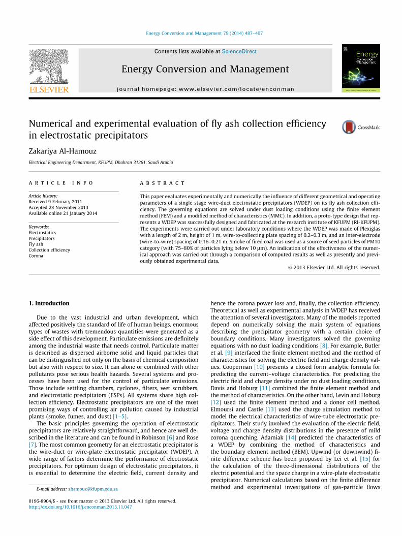
Fig. 1 shows a schematic and top view of a wire-duct electro-static precipitator configuration. When the applied voltage israised, the gas near the more sharply curved wire electrodes breaksdown at a voltage above what is called the onset value and lessthan the spark breakdown value. This incomplete dielectric break-down, which is called a monopolar corona, appears in air as ahighly active region of glow. The monopolar corona within duct-type precipitators includes only positive or negative ions (the backcorona is neglected), the polarity of the ions being the same as thepolarity of the high voltage wires in the corona. In these figures, Ris the wire (electrode) radius, S is the wire-to-plate spacing, D isthe wire to wire spacing and H is the precipitator length.
For this configuration of WDEP, the following system of equa-tions describes the monopolar corona:
r � E*
¼ q=e0 ð1Þ
r � J*
¼ 0 ð2Þ
E!¼ �ru ð3Þ
J!¼ J
!io þ J!
p ð4Þ
J!
io ¼ kioqio E! ð5Þ
J!
p ¼ kpqp E! ð6Þ
where E*
is the electric field intensity vector, q is the total spacecharge density (summation of the ion charge density qio and parti-cle charge density qp, i.e. q ¼ qio þ qp), J
!is the total current den-
sity vector, u is the potential, e0 is the permittivity of free space,and kio and kp are the mobilities for ions and particles, respectively.Eqs. (1)–(6) represent Poisson’s equation, the current continuity
Raw ga
s
Cle
anga
s
HV source
Earthed collectingplate
HV rod with discharging wires
2s
D
H
L
X
Y
A C
Eo
2R
D
S
Dischargingconductor
H
airflow
a
b
Fig. 1. (a) Schematic diagram of a wire-duct electrostatic precipitator (WDEP). (b)Top view of a wire-duct electrostatic precipitator (WDEP).
Z. Al-Hamouz / Energy Conversion and Management 79 (2014) 487–497 489
equation, the field and potential relation, the total current densityequation, and the ion and particle current density equations respec-tively. The exact analytical solution to these equations can only beobtained for parallel plates, coaxial cylinders and concentricspheres. Because of the nature of this problem, a numerical solutionis anticipated as a tool for solving this set of equations. The follow-ing assumptions and boundary conditions are essential require-ments for finding a numerical solution.
2.2. Simplifying assumptions
(1) The influence of particle space charge density on the fieldmay be approximated by assuming that the particle concen-tration Np is constant over a given cross section of the pre-cipitator. The particle’s specific surface Sp (the surface perunit volume of gas) is given as [25]:
Sp ¼ 4Pa2Np ð7Þ
where a is the radius of assumed spherical particles.
The corona discharge is assumed to be distributed uniformlyover the surface of the wires; if the corona electrode has a potentialabove a certain value, called the onset level, the normal componentof the electric field remains constant at the onset value E0, which
ionρρ
FEM Block
To solve Poisson’s Equation (1) (for computing ϕ and E )
E,ϕ
Fig. 2. FEM and the
results from Peek’s derivation and later known as Kaptzov’sassumption [39,40].
(2) The ion mobility is assumed constant.(3) Ion diffusion is ignored.
2.3. Boundary conditions
(1) The potential at the two plates is zero.(2) The potential at the discharging wires is V.(3) The electric field at the discharging wires is E0 which is given
by [40]:
E0 ¼ 3:1� 106 1þ 0:308ffiffiffiffiffiffiffiffiffiffiffiffiffiffiffiffi0:5� Rp
� �ð8Þ
3. Numerical procedure and experimental set-up
3.1. Proposed numerical procedure
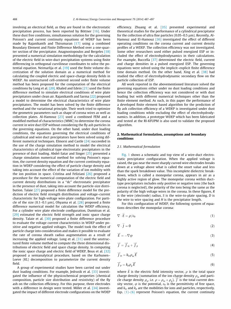
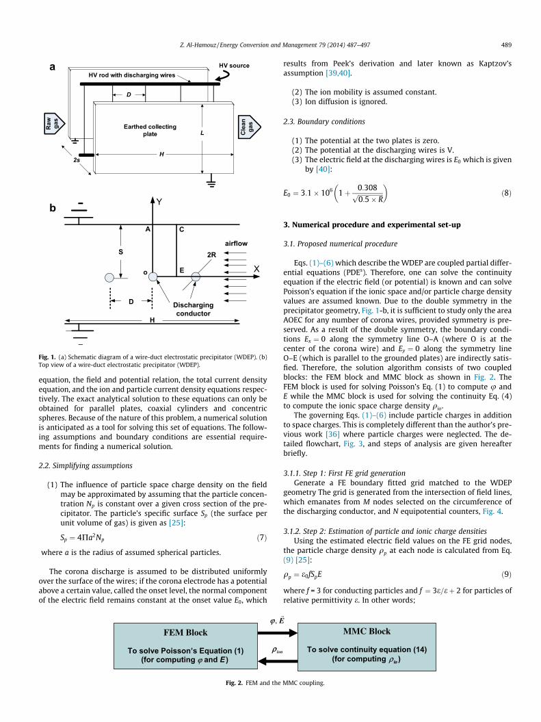
Eqs. (1)–(6) which describe the WDEP are coupled partial differ-ential equations (PDEs). Therefore, one can solve the continuityequation if the electric field (or potential) is known and can solvePoisson’s equation if the ionic space and/or particle charge densityvalues are assumed known. Due to the double symmetry in theprecipitator geometry, Fig. 1-b, it is sufficient to study only the areaAOEC for any number of corona wires, provided symmetry is pre-served. As a result of the double symmetry, the boundary condi-tions Ex ¼ 0 along the symmetry line O–A (where O is at thecenter of the corona wire) and Ey ¼ 0 along the symmetry lineO–E (which is parallel to the grounded plates) are indirectly satis-fied. Therefore, the solution algorithm consists of two coupledblocks: the FEM block and MMC block as shown in Fig. 2. TheFEM block is used for solving Poisson’s Eq. (1) to compute u andE while the MMC block is used for solving the continuity Eq. (4)to compute the ionic space charge density qio.
The governing Eqs. (1)–(6) include particle charges in additionto space charges. This is completely different than the author’s pre-vious work [36] where particle charges were neglected. The de-tailed flowchart, Fig. 3, and steps of analysis are given hereafterbriefly.
3.1.1. Step 1: First FE grid generationGenerate a FE boundary fitted grid matched to the WDEP
geometry The grid is generated from the intersection of field lines,which emanates from M nodes selected on the circumference ofthe discharging conductor, and N equipotential counters, Fig. 4.
3.1.2. Step 2: Estimation of particle and ionic charge densitiesUsing the estimated electric field values on the FE grid nodes,
the particle charge density qp at each node is calculated from Eq.(9) [25]:
qp ¼ e0fSpE ð9Þ
where f = 3 for conducting particles and f ¼ 3e=eþ 2 for particles ofrelative permittivity e. In other words;
MMC Block
To solve continuity equation (14) (for computing ioioρ )
MMC coupling.
Fig. 3. Detailed flowchart of computation.
490 Z. Al-Hamouz / Energy Conversion and Management 79 (2014) 487–497
qp ¼ nE ð10Þ
n ¼ 4Pe0fa2Np ð11Þ
The particle mobility can be calculated as:
kp ¼ qp=6PNpca ð12Þ
where c is the air viscosity.As in [36], a modified method of characteristics (MMC) is used
where the partial differential equation governing the evolution ofcharge density becomes an ordinary differential equation alongspecific ‘‘flux tube’’ trajectories. Therefore, the current continuityequation is written as:
r � J*
¼ r � ðkioqioEþ kpqpEÞ ¼ 0 ð13Þ
To simplify satisfying the continuity condition, particle chargedensity values Jp ¼ kpqpE are assumed constant in each iteration.Therefore, Eq. (13) has been simplified to solve for the ionic spacecharge density values at the FE grid nodes. As a result, Eq. (13) canbe written along each flux tube as:
dqio
dll_
¼ �ðq2io þ qioqpÞ=e0E ð14Þ
where l_
is a unit vector along the axis of the flux tube, that is alongthe direction of E.
3.1.3. Step 3: Finite element solution of Poisson’s equationFor known values of the ionic space charge and particle charge
densities at the FE nodes, Poissions equation, Eq. (1) is solved in thearea AOEC by means of the FEM [41].
3.1.4. Step 4: Particle and space charge density correctionUsing the estimated electric field values at the FE nodes, the par-
ticle charge density at these nodes is updated using Eqs. (9)–(12). Onthe other hand, correction of the ionic space charge density is madeby comparing the computed values of the potential at the kth nodein iterations n and n + 1, as in the following equations:
qi;1ðioÞnew¼ qi;1ðioÞold
½1þ g Fk� i ¼ 1;2; . . . ;M ð15:aÞ
er ¼ junk �unþ1
k j=uav ð15:bÞ
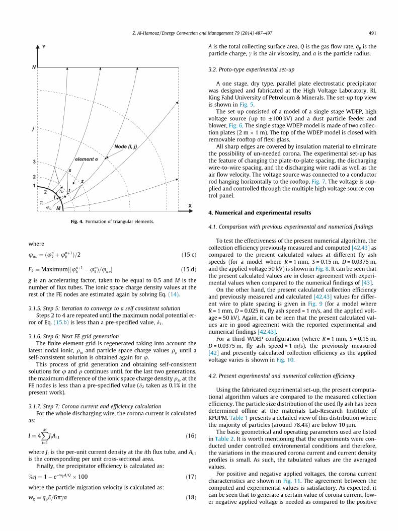
Fig. 4. Formation of triangular elements.
Z. Al-Hamouz / Energy Conversion and Management 79 (2014) 487–497 491
where
uav ¼ ðunk þunþ1
k Þ=2 ð15:cÞ
Fk ¼Maximum½ðunþ1k �un
kÞ=uav � ð15:dÞ
g is an accelerating factor, taken to be equal to 0.5 and M is thenumber of flux tubes. The ionic space charge density values at therest of the FE nodes are estimated again by solving Eq. (14).
3.1.5. Step 5: Iteration to converge to a self consistent solutionSteps 2 to 4 are repeated until the maximum nodal potential er-
ror of Eq. (15.b) is less than a pre-specified value, d1.
3.1.6. Step 6: Next FE grid generationThe finite element grid is regenerated taking into account the
latest nodal ionic, qio and particle space charge values qp until aself-consistent solution is obtained again for u.
This process of grid generation and obtaining self-consistentsolutions for u and q continues until, for the last two generations,the maximum difference of the ionic space charge density qio at theFE nodes is less than a pre-specified value (d2 taken as 0.1% in thepresent work).
3.1.7. Step 7: Corona current and efficiency calculationFor the whole discharging wire, the corona current is calculated
as:
I ¼ 4XM
i¼1
JiAi;1 ð16Þ
where Ji is the per-unit current density at the ith flux tube, and Ai;1
is the corresponding per unit cross-sectional area.Finally, the precipitator efficiency is calculated as:
%g ¼ 1� e�wg A=Q � 100 ð17Þ
where the particle migration velocity is calculated as:
wg ¼ qpE=6pca ð18Þ
A is the total collecting surface area, Q is the gas flow rate, qp is theparticle charge, c is the air viscosity, and a is the particle radius.
3.2. Proto-type experimental set-up
A one stage, dry type, parallel plate electrostatic precipitatorwas designed and fabricated at the High Voltage Laboratory, RI,King Fahd University of Petroleum & Minerals. The set-up top viewis shown in Fig. 5.
The set-up consisted of a model of a single stage WDEP, highvoltage source (up to �100 kV) and a dust particle feeder andblower, Fig. 6. The single stage WDEP model is made of two collec-tion plates (2 m � 1 m). The top of the WDEP model is closed withremovable rooftop of flexi glass.
All sharp edges are covered by insulation material to eliminatethe possibility of un-needed corona. The experimental set-up hasthe feature of changing the plate-to-plate spacing, the dischargingwire-to-wire spacing, and the discharging wire radii as well as theair flow velocity. The voltage source was connected to a conductorrod hanging horizontally to the rooftop, Fig. 7. The voltage is sup-plied and controlled through the multiple high voltage source con-trol panel.
4. Numerical and experimental results
4.1. Comparison with previous experimental and numerical findings
To test the effectiveness of the present numerical algorithm, thecollection efficiency previously measured and computed [42,43] ascompared to the present calculated values at different fly ashspeeds (for a model where R = 1 mm, S = 0.15 m, D = 0.0375 m,and the applied voltage 50 kV) is shown in Fig. 8. It can be seen thatthe present calculated values are in closer agreement with experi-mental values when compared to the numerical findings of [43].
On the other hand, the present calculated collection efficiencyand previously measured and calculated [42,43] values for differ-ent wire to plate spacing is given in Fig. 9 (for a model whereR = 1 mm, D = 0.025 m, fly ash speed = 1 m/s, and the applied volt-age = 50 kV). Again, it can be seen that the present calculated val-ues are in good agreement with the reported experimental andnumerical findings [42,43].
For a third WDEP configuration (where R = 1 mm, S = 0.15 m,D = 0.0375 m, fly ash speed = 1 m/s), the previously measured[42] and presently calculated collection efficiency as the appliedvoltage varies is shown in Fig. 10.
4.2. Present experimental and numerical collection efficiency
Using the fabricated experimental set-up, the present computa-tional algorithm values are compared to the measured collectionefficiency. The particle size distribution of the used fly ash has beendetermined offline at the materials Lab-Research Institute ofKFUPM. Table 1 presents a detailed view of this distribution wherethe majority of particles (around 78.4%) are below 10 lm.
The basic geometrical and operating parameters used are listedin Table 2. It is worth mentioning that the experiments were con-ducted under controlled environmental conditions and therefore,the variations in the measured corona current and current densityprofiles is small. As such, the tabulated values are the averagedvalues.
For positive and negative applied voltages, the corona currentcharacteristics are shown in Fig. 11. The agreement between thecomputed and experimental values is satisfactory. As expected, itcan be seen that to generate a certain value of corona current, low-er negative applied voltage is needed as compared to the positive
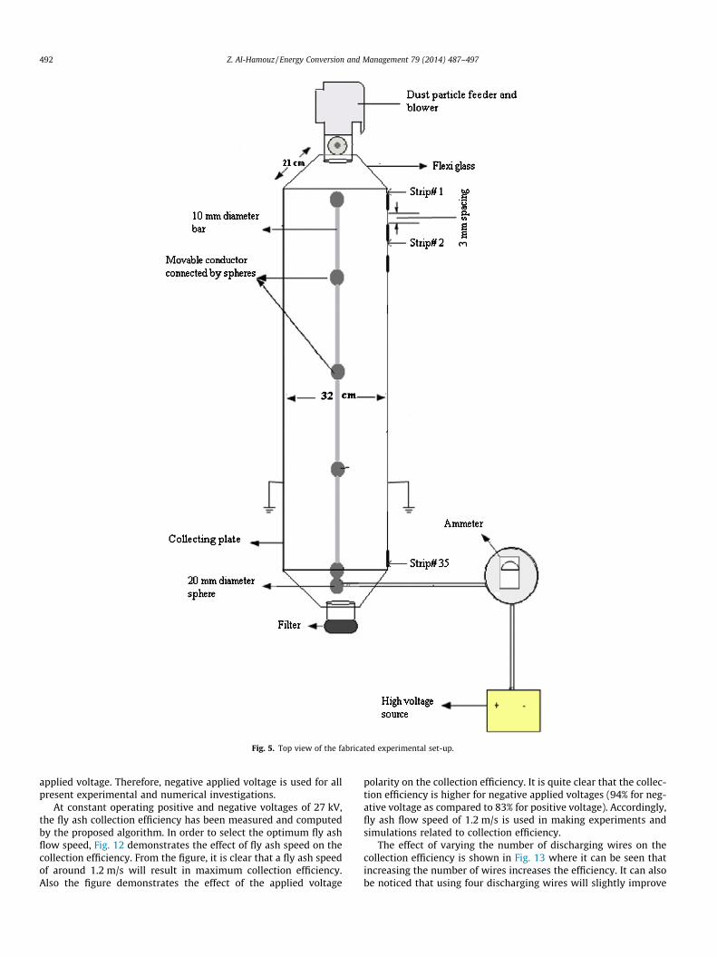
Fig. 5. Top view of the fabricated experimental set-up.
492 Z. Al-Hamouz / Energy Conversion and Management 79 (2014) 487–497
applied voltage. Therefore, negative applied voltage is used for allpresent experimental and numerical investigations.
At constant operating positive and negative voltages of 27 kV,the fly ash collection efficiency has been measured and computedby the proposed algorithm. In order to select the optimum fly ashflow speed, Fig. 12 demonstrates the effect of fly ash speed on thecollection efficiency. From the figure, it is clear that a fly ash speedof around 1.2 m/s will result in maximum collection efficiency.Also the figure demonstrates the effect of the applied voltage
polarity on the collection efficiency. It is quite clear that the collec-tion efficiency is higher for negative applied voltages (94% for neg-ative voltage as compared to 83% for positive voltage). Accordingly,fly ash flow speed of 1.2 m/s is used in making experiments andsimulations related to collection efficiency.
The effect of varying the number of discharging wires on thecollection efficiency is shown in Fig. 13 where it can be seen thatincreasing the number of wires increases the efficiency. It can alsobe noticed that using four discharging wires will slightly improve
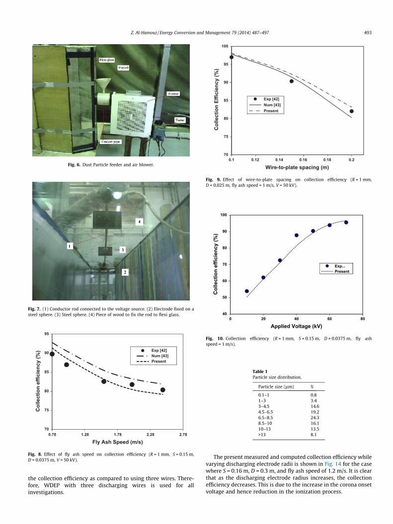
Fig. 6. Dust Particle feeder and air blower.
Fig. 7. (1) Conductor rod connected to the voltage source. (2) Electrode fixed on asteel sphere. (3) Steel sphere. (4) Piece of wood to fix the rod to flexi glass.
70
75
80
85
90
95
0.78 1.28 1.78 2.28 2.78
Col
lect
ion
effic
ienc
y (%
)
Fly Ash Speed (m/s)
Exp [42]Num [43]Present
Fig. 8. Effect of fly ash speed on collection efficiency (R = 1 mm, S = 0.15 m,D = 0.0375 m, V = 50 kV).
70
75
80
85
90
95
100
0.1 0.12 0.14 0.16 0.18 0.2
Col
lect
ion
Effic
ienc
y (%
)
Wire-to-plate spacing (m)
Exp [42]Num [43]Present
Fig. 9. Effect of wire-to-plate spacing on collection efficiency (R = 1 mm,D = 0.025 m, fly ash speed = 1 m/s, V = 50 kV).
40
50
60
70
80
90
100
0 20 40 60 80
Col
lect
ion
effic
ienc
y (%
)
Applied Voltage (kV)
Exp… Present
Fig. 10. Collection efficiency (R = 1 mm, S = 0.15 m, D = 0.0375 m, fly ashspeed = 1 m/s).
Table 1Particle size distribution.
Particle size (lm) %
0.1–1 0.81–3 3.43–4.5 14.64.5–6.5 19.26.5–8.5 24.38.5–10 16.110–13 13.5>13 8.1
Z. Al-Hamouz / Energy Conversion and Management 79 (2014) 487–497 493
the collection efficiency as compared to using three wires. There-fore, WDEP with three discharging wires is used for allinvestigations.
The present measured and computed collection efficiency whilevarying discharging electrode radii is shown in Fig. 14 for the casewhere S = 0.16 m, D = 0.3 m, and fly ash speed of 1.2 m/s. It is clearthat as the discharging electrode radius increases, the collectionefficiency decreases. This is due to the increase in the corona onsetvoltage and hence reduction in the ionization process.
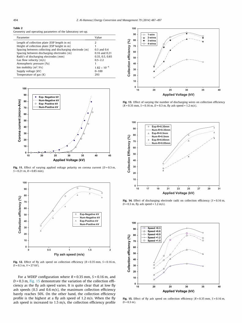
Table 2Geometry and operating parameters of the laboratory set-up.
Parameter Value
Length of collection plate (ESP length in m) 2Height of collection plate (ESP height in m) 1Spacing between collecting and discharging electrode (m) 0.3 and 0.4Spacing between discharging electrodes (m) 0.16 and 0.21Radii’s of discharging electrodes (mm) 0.35, 0.5, 0.85Gas flow velocity (m/s) 0.5–2.2Atmospheric pressure (Pa) 1Ion mobility (m2=Vs) 1:82� 10�4
Supply voltage (kV) 0–100Temperature of gas (K) 293
0
10
20
30
40
50
60
70
80
90
100
15 20 25 30 35 40 45
Applied Voltage (kV)
Cor
ona
curr
ent (
mic
ro-A
/m)
Exp- Negative kVNum-Negative kVExp- Positive kVNum-Positive kV
Fig. 11. Effect of varying applied voltage polarity on corona current (D = 0.3 m,S = 0.21 m, R = 0.85 mm).
0
10
20
30
40
50
60
70
80
90
100
0 0.5 1 1.5 2
Fly ash speed (m/s)
Col
lect
ion
effic
ienc
y (%
)
Exp-Negative kVNum-Negative kVExp-Positive kVNum-Positive kV
Fig. 12. Effect of fly ash speed on collection efficiency (R = 0.35 mm, S = 0.16 m,D = 0.3 m, V = 27 kV).
0
10
20
30
40
50
60
70
80
90
100
15 20 25 30 35 40
Applied Voltage (kV)
Col
lect
ion
effic
ienc
y (%
)
1-wire2-wires3-wires4-wires
Fig. 13. Effect of varying the number of discharging wires on collection efficiency(R = 0.35 mm, S = 0.16 m, D = 0.3 m, fly ash speed = 1.2 m/s).
0
10
20
30
40
50
60
70
80
90
100
15 17 19 21 23 25 27 29 31
Applied Voltage (kV)
Col
lect
ion
Effic
ienc
y (%
)Exp-R=0.35mmNum-R=0.35mmExp-R=0.5mmNum-R=0.5mmExp-R=0.85mmNum-R=0.85mm
Fig. 14. Effect of discharging electrode radii on collection efficiency (S = 0.16 m,D = 0.3 m, fly ash speed = 1.2 m/s).
0
10
20
30
40
50
60
70
80
90
100
15 20 25 30 35 40
Applied Voltage (kV)
Col
lect
ion
effic
ienc
y (%
)
Speed =0.3Speed =0.6Speed =0.9Speed =1.2Speed =1.5
Fig. 15. Effect of fly ash speed on collection efficiency (R = 0.35 mm, S = 0.16 m,D = 0.3 m).
494 Z. Al-Hamouz / Energy Conversion and Management 79 (2014) 487–497
For a WDEP configuration where R = 0.35 mm, S = 0.16 m, andD = 0.3 m, Fig. 15 demonstrate the variation of the collection effi-ciency as the fly ash speed varies. It is quite clear that at low flyash speeds (0.3 and 0.6 m/s), the maximum collection efficiencybarely reaches 50%. On the other hand, the collection efficiencyprofile is the highest at a fly ash speed of 1.2 m/s. When the flyash speed is increased to 1.5 m/s, the collection efficiency profile
0
10
20
30
40
50
60
70
80
90
100
18 19 20 21 22 23 24 25 26 27
Applied Voltage (kV)
Col
lect
ion
Effic
ienc
y (%
)
Exp-D=0.4mNum-D=0.4mExp-D=0.3mNum-D=0.3m
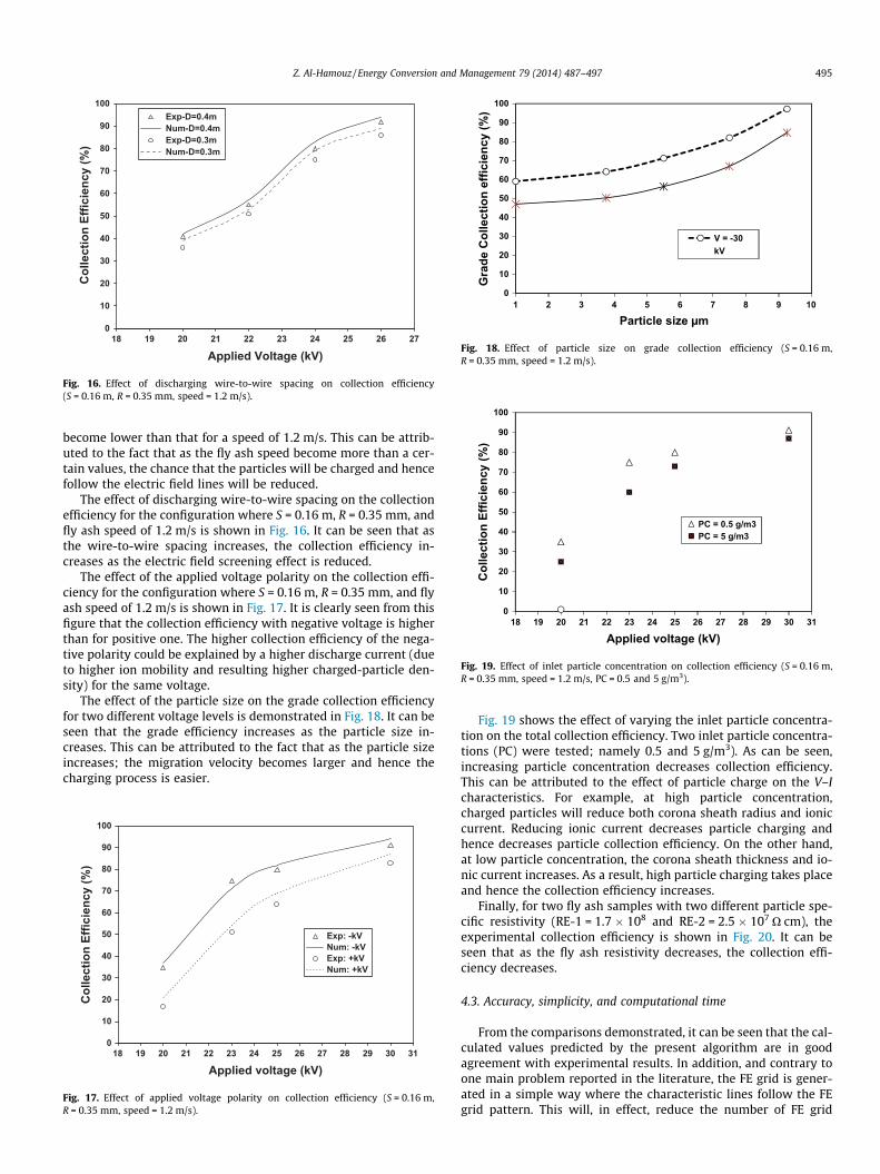
Fig. 16. Effect of discharging wire-to-wire spacing on collection efficiency(S = 0.16 m, R = 0.35 mm, speed = 1.2 m/s).
0
10
20
30
40
50
60
70
80
90
100
1 2 3 4 5 6 7 8 9 10
Gra
de C
olle
ctio
n ef
ficie
ncy
(%)
Particle size µm
V = -30 kV
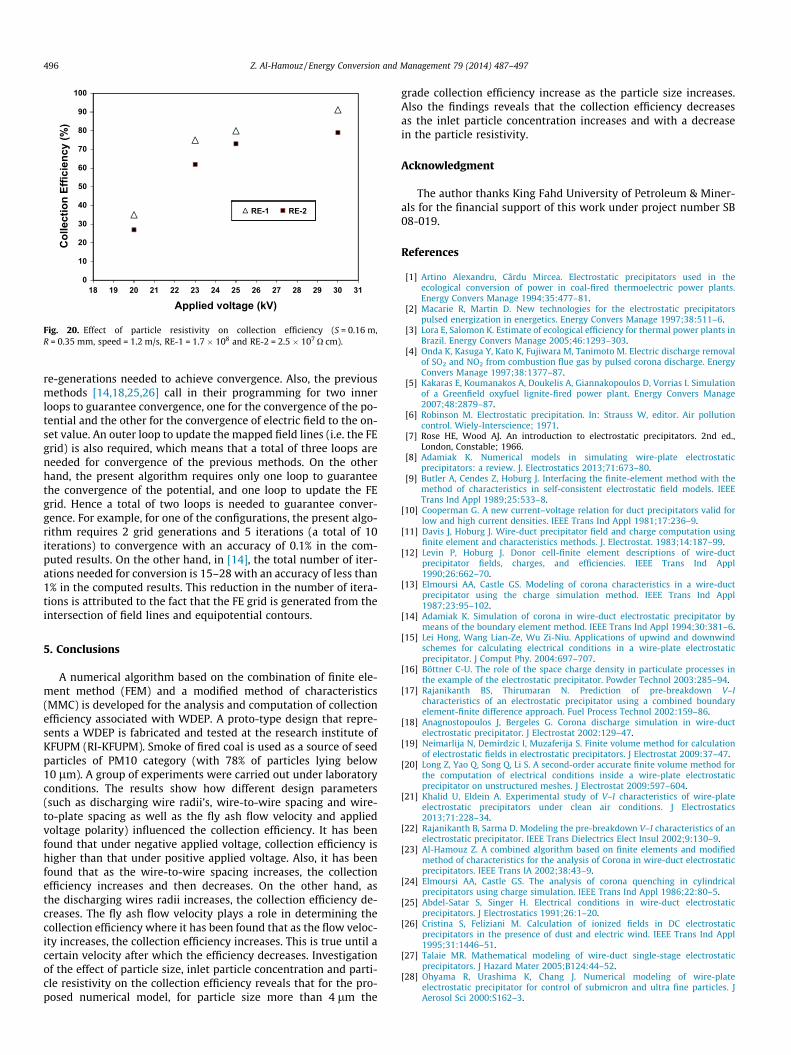
Fig. 18. Effect of particle size on grade collection efficiency (S = 0.16 m,R = 0.35 mm, speed = 1.2 m/s).
0
10
20
30
40
50
60
70
80
90
100
18 19 20 21 22 23 24 25 26 27 28 29 30 31
Col
lect
ion
Effic
ienc
y (%
)
Applied voltage (kV)
PC = 0.5 g/m3PC = 5 g/m3
Fig. 19. Effect of inlet particle concentration on collection efficiency (S = 0.16 m,R = 0.35 mm, speed = 1.2 m/s, PC = 0.5 and 5 g/m3).
Z. Al-Hamouz / Energy Conversion and Management 79 (2014) 487–497 495
become lower than that for a speed of 1.2 m/s. This can be attrib-uted to the fact that as the fly ash speed become more than a cer-tain values, the chance that the particles will be charged and hencefollow the electric field lines will be reduced.
The effect of discharging wire-to-wire spacing on the collectionefficiency for the configuration where S = 0.16 m, R = 0.35 mm, andfly ash speed of 1.2 m/s is shown in Fig. 16. It can be seen that asthe wire-to-wire spacing increases, the collection efficiency in-creases as the electric field screening effect is reduced.
The effect of the applied voltage polarity on the collection effi-ciency for the configuration where S = 0.16 m, R = 0.35 mm, and flyash speed of 1.2 m/s is shown in Fig. 17. It is clearly seen from thisfigure that the collection efficiency with negative voltage is higherthan for positive one. The higher collection efficiency of the nega-tive polarity could be explained by a higher discharge current (dueto higher ion mobility and resulting higher charged-particle den-sity) for the same voltage.
The effect of the particle size on the grade collection efficiencyfor two different voltage levels is demonstrated in Fig. 18. It can beseen that the grade efficiency increases as the particle size in-creases. This can be attributed to the fact that as the particle sizeincreases; the migration velocity becomes larger and hence thecharging process is easier.
0
10
20
30
40
50
60
70
80
90
100
18 19 20 21 22 23 24 25 26 27 28 29 30 31
Applied voltage (kV)
Col
lect
ion
Effic
ienc
y (%
)
Exp: -kVNum: -kVExp: +kVNum: +kV
Fig. 17. Effect of applied voltage polarity on collection efficiency (S = 0.16 m,R = 0.35 mm, speed = 1.2 m/s).
Fig. 19 shows the effect of varying the inlet particle concentra-tion on the total collection efficiency. Two inlet particle concentra-tions (PC) were tested; namely 0.5 and 5 g/m3). As can be seen,increasing particle concentration decreases collection efficiency.This can be attributed to the effect of particle charge on the V–Icharacteristics. For example, at high particle concentration,charged particles will reduce both corona sheath radius and ioniccurrent. Reducing ionic current decreases particle charging andhence decreases particle collection efficiency. On the other hand,at low particle concentration, the corona sheath thickness and io-nic current increases. As a result, high particle charging takes placeand hence the collection efficiency increases.
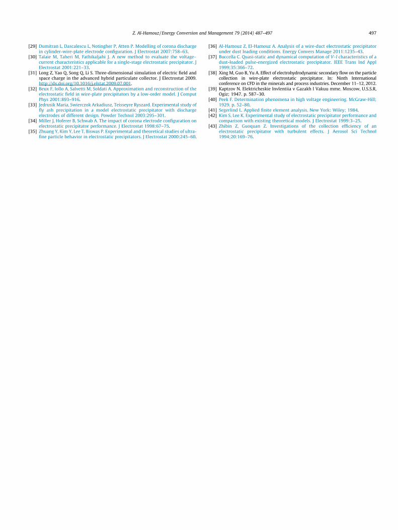
Finally, for two fly ash samples with two different particle spe-cific resistivity (RE-1 = 1.7 � 108 and RE-2 = 2.5 � 107 O cm), theexperimental collection efficiency is shown in Fig. 20. It can beseen that as the fly ash resistivity decreases, the collection effi-ciency decreases.
4.3. Accuracy, simplicity, and computational time
From the comparisons demonstrated, it can be seen that the cal-culated values predicted by the present algorithm are in goodagreement with experimental results. In addition, and contrary toone main problem reported in the literature, the FE grid is gener-ated in a simple way where the characteristic lines follow the FEgrid pattern. This will, in effect, reduce the number of FE grid
0
10
20
30
40
50
60
70
80
90
100
18 19 20 21 22 23 24 25 26 27 28 29 30 31
Col
lect
ion
Effic
ienc
y (%
)
Applied voltage (kV)
RE-1 RE-2
Fig. 20. Effect of particle resistivity on collection efficiency (S = 0.16 m,R = 0.35 mm, speed = 1.2 m/s, RE-1 = 1.7 � 108 and RE-2 = 2.5 � 107 O cm).
496 Z. Al-Hamouz / Energy Conversion and Management 79 (2014) 487–497
re-generations needed to achieve convergence. Also, the previousmethods [14,18,25,26] call in their programming for two innerloops to guarantee convergence, one for the convergence of the po-tential and the other for the convergence of electric field to the on-set value. An outer loop to update the mapped field lines (i.e. the FEgrid) is also required, which means that a total of three loops areneeded for convergence of the previous methods. On the otherhand, the present algorithm requires only one loop to guaranteethe convergence of the potential, and one loop to update the FEgrid. Hence a total of two loops is needed to guarantee conver-gence. For example, for one of the configurations, the present algo-rithm requires 2 grid generations and 5 iterations (a total of 10iterations) to convergence with an accuracy of 0.1% in the com-puted results. On the other hand, in [14], the total number of iter-ations needed for conversion is 15–28 with an accuracy of less than1% in the computed results. This reduction in the number of itera-tions is attributed to the fact that the FE grid is generated from theintersection of field lines and equipotential contours.
5. Conclusions
A numerical algorithm based on the combination of finite ele-ment method (FEM) and a modified method of characteristics(MMC) is developed for the analysis and computation of collectionefficiency associated with WDEP. A proto-type design that repre-sents a WDEP is fabricated and tested at the research institute ofKFUPM (RI-KFUPM). Smoke of fired coal is used as a source of seedparticles of PM10 category (with 78% of particles lying below10 lm). A group of experiments were carried out under laboratoryconditions. The results show how different design parameters(such as discharging wire radii’s, wire-to-wire spacing and wire-to-plate spacing as well as the fly ash flow velocity and appliedvoltage polarity) influenced the collection efficiency. It has beenfound that under negative applied voltage, collection efficiency ishigher than that under positive applied voltage. Also, it has beenfound that as the wire-to-wire spacing increases, the collectionefficiency increases and then decreases. On the other hand, asthe discharging wires radii increases, the collection efficiency de-creases. The fly ash flow velocity plays a role in determining thecollection efficiency where it has been found that as the flow veloc-ity increases, the collection efficiency increases. This is true until acertain velocity after which the efficiency decreases. Investigationof the effect of particle size, inlet particle concentration and parti-cle resistivity on the collection efficiency reveals that for the pro-posed numerical model, for particle size more than 4 lm the
grade collection efficiency increase as the particle size increases.Also the findings reveals that the collection efficiency decreasesas the inlet particle concentration increases and with a decreasein the particle resistivity.
Acknowledgment
The author thanks King Fahd University of Petroleum & Miner-als for the financial support of this work under project number SB08-019.
References
[1] Artino Alexandru, Cârdu Mircea. Electrostatic precipitators used in theecological conversion of power in coal-fired thermoelectric power plants.Energy Convers Manage 1994;35:477–81.
[2] Macarie R, Martin D. New technologies for the electrostatic precipitatorspulsed energization in energetics. Energy Convers Manage 1997;38:511–6.
[3] Lora E, Salomon K. Estimate of ecological efficiency for thermal power plants inBrazil. Energy Convers Manage 2005;46:1293–303.
[4] Onda K, Kasuga Y, Kato K, Fujiwara M, Tanimoto M. Electric discharge removalof SO2 and NO2 from combustion flue gas by pulsed corona discharge. EnergyConvers Manage 1997;38:1377–87.
[5] Kakaras E, Koumanakos A, Doukelis A, Giannakopoulos D, Vorrias I. Simulationof a Greenfield oxyfuel lignite-fired power plant. Energy Convers Manage2007;48:2879–87.
[6] Robinson M. Electrostatic precipitation. In: Strauss W, editor. Air pollutioncontrol. Wiely-Interscience; 1971.
[7] Rose HE, Wood AJ. An introduction to electrostatic precipitators. 2nd ed.,London, Constable; 1966.
[8] Adamiak K. Numerical models in simulating wire-plate electrostaticprecipitators: a review. J. Electrostatics 2013;71:673–80.
[9] Butler A, Cendes Z, Hoburg J. Interfacing the finite-element method with themethod of characteristics in self-consistent electrostatic field models. IEEETrans Ind Appl 1989;25:533–8.
[10] Cooperman G. A new current–voltage relation for duct precipitators valid forlow and high current densities. IEEE Trans Ind Appl 1981;17:236–9.
[11] Davis J, Hoburg J. Wire-duct precipitator field and charge computation usingfinite element and characteristics methods. J. Electrostat. 1983;14:187–99.
[12] Levin P, Hoburg J. Donor cell-finite element descriptions of wire-ductprecipitator fields, charges, and efficiencies. IEEE Trans Ind Appl1990;26:662–70.
[13] Elmoursi AA, Castle GS. Modeling of corona characteristics in a wire-ductprecipitator using the charge simulation method. IEEE Trans Ind Appl1987;23:95–102.
[14] Adamiak K. Simulation of corona in wire-duct electrostatic precipitator bymeans of the boundary element method. IEEE Trans Ind Appl 1994;30:381–6.
[15] Lei Hong, Wang Lian-Ze, Wu Zi-Niu. Applications of upwind and downwindschemes for calculating electrical conditions in a wire-plate electrostaticprecipitator. J Comput Phy. 2004:697–707.
[16] Böttner C-U. The role of the space charge density in particulate processes inthe example of the electrostatic precipitator. Powder Technol 2003:285–94.
[17] Rajanikanth BS, Thirumaran N. Prediction of pre-breakdown V–Icharacteristics of an electrostatic precipitator using a combined boundaryelement-finite difference approach. Fuel Process Technol 2002:159–86.
[18] Anagnostopoulos J, Bergeles G. Corona discharge simulation in wire-ductelectrostatic precipitator. J Electrostat 2002:129–47.
[19] Neimarlija N, Demirdzic I, Muzaferija S. Finite volume method for calculationof electrostatic fields in electrostatic precipitators. J Electrostat 2009:37–47.
[20] Long Z, Yao Q, Song Q, Li S. A second-order accurate finite volume method forthe computation of electrical conditions inside a wire-plate electrostaticprecipitator on unstructured meshes. J Electrostat 2009:597–604.
[21] Khalid U, Eldein A. Experimental study of V–I characteristics of wire-plateelectrostatic precipitators under clean air conditions. J Electrostatics2013;71:228–34.
[22] Rajanikanth B, Sarma D. Modeling the pre-breakdown V–I characteristics of anelectrostatic precipitator. IEEE Trans Dielectrics Elect Insul 2002;9:130–9.
[23] Al-Hamouz Z. A combined algorithm based on finite elements and modifiedmethod of characteristics for the analysis of Corona in wire-duct electrostaticprecipitators. IEEE Trans IA 2002;38:43–9.
[24] Elmoursi AA, Castle GS. The analysis of corona quenching in cylindricalprecipitators using charge simulation. IEEE Trans Ind Appl 1986;22:80–5.
[25] Abdel-Satar S, Singer H. Electrical conditions in wire-duct electrostaticprecipitators. J Electrostatics 1991;26:1–20.
[26] Cristina S, Feliziani M. Calculation of ionized fields in DC electrostaticprecipitators in the presence of dust and electric wind. IEEE Trans Ind Appl1995;31:1446–51.
[27] Talaie MR. Mathematical modeling of wire-duct single-stage electrostaticprecipitators. J Hazard Mater 2005;B124:44–52.
[28] Ohyama R, Urashima K, Chang J. Numerical modeling of wire-plateelectrostatic precipitator for control of submicron and ultra fine particles. JAerosol Sci 2000:S162–3.
Z. Al-Hamouz / Energy Conversion and Management 79 (2014) 487–497 497
[29] Dumitran L, Dascalescu L, Notingher P, Atten P. Modelling of corona dischargein cylinder-wire-plate electrode configuration. J Electrostat 2007:758–63.
[30] Talaie M, Taheri M, Fathikaljahi J. A new method to evaluate the voltage–current characteristics applicable for a single-stage electrostatic precipitator. JElectrostat 2001:221–33.
[31] Long Z, Yao Q, Song Q, Li S. Three-dimensional simulation of electric field andspace charge in the advanced hybrid particulate collector. J Electrostat 2009.http://dx.doi.org/10.1016/j.elstat.2009.07.001.
[32] Beux F, Iollo A, Salvetti M, Soldati A. Approximation and reconstruction of theelectrostatic field in wire-plate precipitators by a low-order model. J ComputPhys 2001:893–916.
[33] Jedrusik Maria, Swierczok Arkadiusz, Teisseyre Ryszard. Experimental study offly ash precipitation in a model electrostatic precipitator with dischargeelectrodes of different design. Powder Technol 2003:295–301.
[34] Miller J, Hoferer B, Schwab A. The impact of corona electrode configuration onelectrostatic precipitator performance. J Electrostat 1998:67–75.
[35] Zhuang Y, Kim Y, Lee T, Biswas P. Experimental and theoretical studies of ultra-fine particle behavior in electrostatic precipitators. J Electrostat 2000:245–60.
[36] Al-Hamouz Z, El-Hamouz A. Analysis of a wire-duct electrostatic precipitatorunder dust loading conditions. Energy Convers Manage 2011:1235–43.
[37] Buccella C. Quasi-static and dynamical computation of V–I characteristics of adust-loaded pulse-energized electrostatic precipitator. IEEE Trans Ind Appl1999;35:366–72.
[38] Xing M, Guo B, Yu A. Effect of electrohydrodynamic secondary flow on the particlecollection in wire-plate electrostatic precipitator. In: Ninth Internationalconference on CFD in the minerals and process industries. December 11–12, 2012.
[39] Kaptzov N. Elektricheskie Invlentiia v Gazakh I Vakuu mme. Moscow, U.S.S.R,Ogiz; 1947. p. 587–30.
[40] Peek F. Determination phenomena in high voltage engineering. McGraw-Hill;1929. p. 52–80.
[41] Segerlind L. Applied finite element analysis. New York: Wiley; 1984.[42] Kim S, Lee K. Experimental study of electrostatic precipitator performance and
comparison with existing theoretical models. J Electrostat 1999:3–25.[43] Zhibin Z, Guoquan Z. Investigations of the collection efficiency of an
electrostatic precipitator with turbulent effects. J Aerosol Sci Technol1994;20:169–76.