12th IMEKO TC1 & TC7 Joint Symposium on Man Science & Measurement

September, 3 – 5, 2008, Annecy, France

NOVEL METHOD FOR INLINE ESTIMATION OF PROBING UNCERTAINTY

IN OPTICAL MEASUREMENT G. Linß, S.C.N. Töpfer

Technische Universität Ilmenau, Ilmenau, Germany, Gerhard.Linss@TU-Ilmenau.de

Abstract: Typically measuring points in optical coordinate metrology are considered equally at the subsequent fitting of geometric elements, for example circle. Thereby it is assumed that the related probing uncertainty does neither vary locally nor between different measuring objects. This paper outlines a novel approach for the determination of quality measures as a measure for the related probing uncertainty. The quality measures are based on the quantitative evaluation of the intensity characteristic at the edge, whose position is to be measured. Thereby five different criteria such as slope, width, form, noise and uniqueness of the edge are utilised. The overall quality measure is calculated as a weighted sum of the individual quality measures. The proposed quality measures have been applied at a number of different measuring objects. The experimental data prove the soundness of the new approach. The utilisation of the proposed quality measures results in a decrease of measuring uncertainty.

Keywords: optical measurement, contour point, probing uncertainty

1. INTRODUCTION

Typically dimensional measurements with optical coordinate measuring machines (CMM) are aiming at the measurement of geometric elements. The geometric elements, for example circle, are utilised in order to describe the shape and dimension of the inspected measuring object respectively of its inspection features. Thereby the parameters of the geometric elements are calculated from the measured contour points. Dimensional measurements with imaging sensors are characterised by measuring contour points in the area of interest (AOI) in the captured image. When calculating the geometric elements different fitting methods are utilised, for example Gaussian least squares method or Chebyshev method such as maximum inscribed circle [1]. Additionally various methods for outlier elimination [3] exist. Very often these methods are applied before fitting the geometric elements to the measured contour points or as part of it.

The state-of-the-art is represented by the equal utilisation of all measured contour points for calculating the geometric elements. A comprehensive internet, literature and patent search yielded no result regarding a method for determining the probing uncertainty of individual contour points in the

field of optical coordinate metrology. This paper proposes a novel method to calculate a set of quality measures in order to supplement each measured contour point with quantitative information about its related probing uncertainty. Fundamental working principle of our method is the analysis of the intensity characteristic at the edge. For the probing uncertainty can greatly vary locally it is desirable to perform an inline estimation of the probing uncertainty.

This paper describes various methods to specify the probing uncertainty in section 2. The next section outlines the steps which are required to perform dimensional measurements with imaging sensors. Thereby different causes for the variation of the probing uncertainty are explained. Section 4 describes in detail the calculation of the proposed set of quality measures. Afterwards the attained experimental results are discussed in section 5. Finally, the paper closes with a concise summary.

2. PROBING UNCERTAINTY

The two-dimensional probing uncertainty, denoted as probing error R2, is specified in the VDI 2617 part 6 guideline [5]. This guideline states that the probing error of a CMM comprises the random scatter of the CMM and particularly the probing error of the sensor deployed for probing. If imaging sensors are utilised as probing sensor there are two principal operation modi available. Measurements can be performed either without moving the CMM axes or with moving the CMM axes. Consequently, the probing error has to be specified separately for each operation mode. The probing error R2 is defined as the range of the radial distance of the measured contour points to the mathe-matically calculated circle using the Gaussian least squares method as fitting procedure [5]. Thereby circular standards, for example even chrome ring structures, with a concentricity deviation of less than one fifth of R2 are deployed in level arrangement. At least 15 measuring points, which have to be distributed uniformly on the circumference of the circle, are acquired [5].

A more recent method to specify the two-dimensional probing uncertainty, denoted as maximum permissible error MPEp, is described in the ISO 10360-2 guideline [7]. For the ISO 10360 guidelines are focused on touch probe sensors the VDI 2617 part 6.1 guideline [6], which is

103

focusing on CMMs with optical sensors, has been created. Therein the two-dimensional probing uncertainty, denoted as PF2D, is similarly defined to R2, but 25 measuring points have to be acquired. Thereby the analysis regions resp. AOIs for each measuring point must not overlap. The two operation modi are differed by specifying PF2D-(OS) for static measurements and specifying PF2D-(OT) for measurements with translatory movement of the CMM.

However, all guidelines for specification of the probing uncertainty for imaging sensors have one common lack. The determination of the probing uncertainty is always performed on measuring objects with ideal characteristics. Thus, such a specification of the probing uncertainty gives an idea how the CMM will perform at ideal measuring objects. In contrast to this, there is a large variety of measuring objects with different characteristics which are inspected in industry. As most of the measuring objects have no ideal characteristics the actual probing uncertainty is worse than the specified probing uncertainty. This is especially true if measurements are performed in top light.

3. INFLUENCES ON OPTICAL MEASUREMENTS

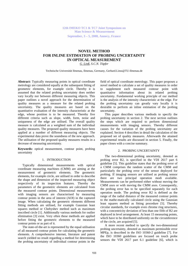
In contrast to dimensional measurements with touch probes the number of parameters for dimensional measurements with imaging sensors is much larger (Fig. 1). Before performing a measurement these parameters have to be adjusted which is done preferably in the sequence depicted in Fig. 1. Thereby the classification of edge detection criteria and subpixel methods is derived from [Kühn 97]. Based on the experience of the operator of an optical CMM the parameter adjustments are either optimal or inappropriate. The latter leads to the occurrence of large deviations of the measuring result from its true value.

Fig. 1. Parameters for dimensional measurements with imaging

Depending on the chosen parameter settings the probing

uncertainty can greatly vary. Exemplarily the probing uncertainty can be significantly increased if a measuring object is measured in top light instead of being measured in transmitted light. Likewise the probing uncertainty can be significantly increased when the chosen probing direction or edge detection criterion is inappropriate. The dependence of the actual probing uncertainty on various parameters poses a specific challenge in dimensional measurements with imaging sensors. It also drives the need to estimate the probing uncertainty inline.

4. CALCULATION OF QUALITY MEASURES FOR PROBING

The aim of the proposed quality measures is the evaluation of the intensity characteristic regarding its suitability for highly precise edge detection. Highly precise edge detection is linked to a minimum probing uncertainty of the measured contour points. The proposed quality measures are targeting the achievement of minimum stochastic measurement deviations. Systematic measurement deviations are not covered by this approach, for these are per definition determined and eliminated through suitable calibration and correction procedures.

Basically the overall quality measure for the edge quality QK may be composed of any set of individual quality measures. This paper proposes a set of five different quality measures. These are uniqueness (QE), form (QF), slope (QA), noise (QR) and width (QB) of the edge. The working principle of the different criteria is illustrated in Fig. 2.

Fig. 2. Determination of the edge quality at a typical intensity curve

at an edge captured in incident light

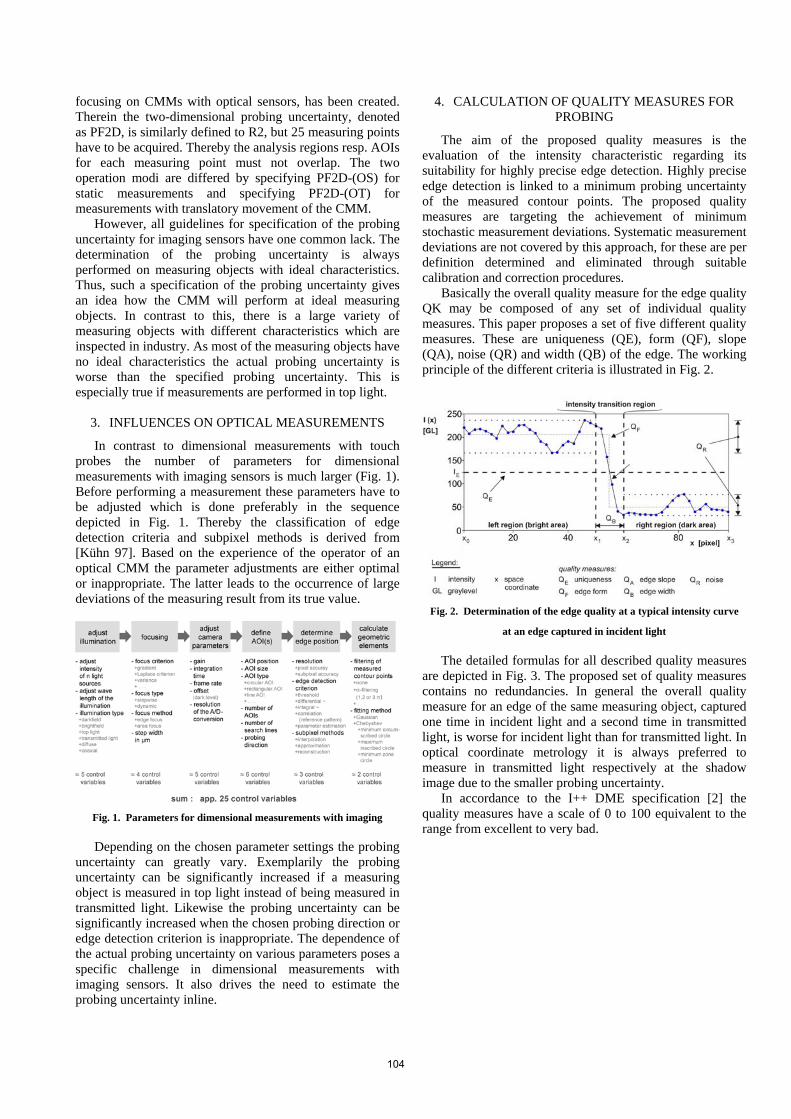
The detailed formulas for all described quality measures are depicted in Fig. 3. The proposed set of quality measures contains no redundancies. In general the overall quality measure for an edge of the same measuring object, captured one time in incident light and a second time in transmitted light, is worse for incident light than for transmitted light. In optical coordinate metrology it is always preferred to measure in transmitted light respectively at the shadow image due to the smaller probing uncertainty.

In accordance to the I++ DME specification [2] the quality measures have a scale of 0 to 100 equivalent to the range from excellent to very bad.

104

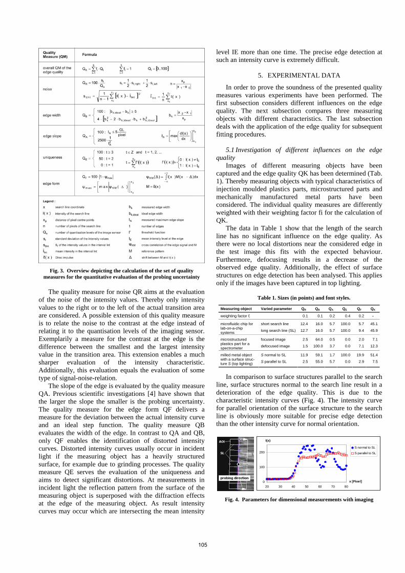
Fig. 3. Overview depicting the calculation of the set of quality

measures for the quantitative evaluation of the probing uncertainty

The quality measure for noise QR aims at the evaluation of the noise of the intensity values. Thereby only intensity values to the right or to the left of the actual transition area are considered. A possible extension of this quality measure is to relate the noise to the contrast at the edge instead of relating it to the quantisation levels of the imaging sensor. Exemplarily a measure for the contrast at the edge is the difference between the smallest and the largest intensity value in the transition area. This extension enables a much sharper evaluation of the intensity characteristic. Additionally, this evaluation equals the evaluation of some type of signal-noise-relation.

The slope of the edge is evaluated by the quality measure QA. Previous scientific investigations [4] have shown that the larger the slope the smaller is the probing uncertainty. The quality measure for the edge form QF delivers a measure for the deviation between the actual intensity curve and an ideal step function. The quality measure QB evaluates the width of the edge. In contrast to QA and QB, only QF enables the identification of distorted intensity curves. Distorted intensity curves usually occur in incident light if the measuring object has a heavily structured surface, for example due to grinding processes. The quality measure QE serves the evaluation of the uniqueness and aims to detect significant distortions. At measurements in incident light the reflection pattern from the surface of the measuring object is superposed with the diffraction effects at the edge of the measuring object. As result intensity curves may occur which are intersecting the mean intensity

level IE more than one time. The precise edge detection at such an intensity curve is extremely difficult.

5. EXPERIMENTAL DATA

In order to prove the soundness of the presented quality measures various experiments have been performed. The first subsection considers different influences on the edge quality. The next subsection compares three measuring objects with different characteristics. The last subsection deals with the application of the edge quality for subsequent fitting procedures.

5.1 Investigation of different influences on the edge quality

Images of different measuring objects have been captured and the edge quality QK has been determined (Tab. 1). Thereby measuring objects with typical characteristics of injection moulded plastics parts, microstructured parts and mechanically manufactured metal parts have been considered. The individual quality measures are differently weighted with their weighting factor fi for the calculation of QK.

The data in Table 1 show that the length of the search line has no significant influence on the edge quality. As there were no local distortions near the considered edge in the test image this fits with the expected behaviour. Furthermore, defocusing results in a decrease of the observed edge quality. Additionally, the effect of surface structures on edge detection has been analysed. This applies only if the images have been captured in top lighting.

Table 1. Sizes (in points) and font styles.

Measuring object Varied parameter QR QB QA QE QF QK

weighting factor fi 0.1 0.1 0.2 0.4 0.2 -

short search line 12.4 16.0 5.7 100.0 5.7 45.1microfluidic chip for lab-on-a-chip systems long search line (SL) 12.7 16.0 5.7 100.0 9.4 45.9

focused image 2.5 64.0 0.5 0.0 2.0 7.1microstructured plastics part for a spectrometer defocused image 1.5 100.0 3.7 0.0 7.1 12.3

S normal to SL 11.9 59.1 1.7 100.0 19.9 51.4milled metal object with a surface struc-ture S (top lighting) S parallel to SL 2.5 55.0 5.7 0.0 2.9 7.5

In comparison to surface structures parallel to the search

line, surface structures normal to the search line result in a deterioration of the edge quality. This is due to the characteristic intensity curves (Fig. 4). The intensity curve for parallel orientation of the surface structure to the search line is obviously more suitable for precise edge detection than the other intensity curve for normal orientation.

0

100

200

20 30 40 50 60 70 80x [Pixel]

I(x)

S normal to SL

S parallel to SL

Fig. 4. Parameters for dimensional measurements with imaging

105

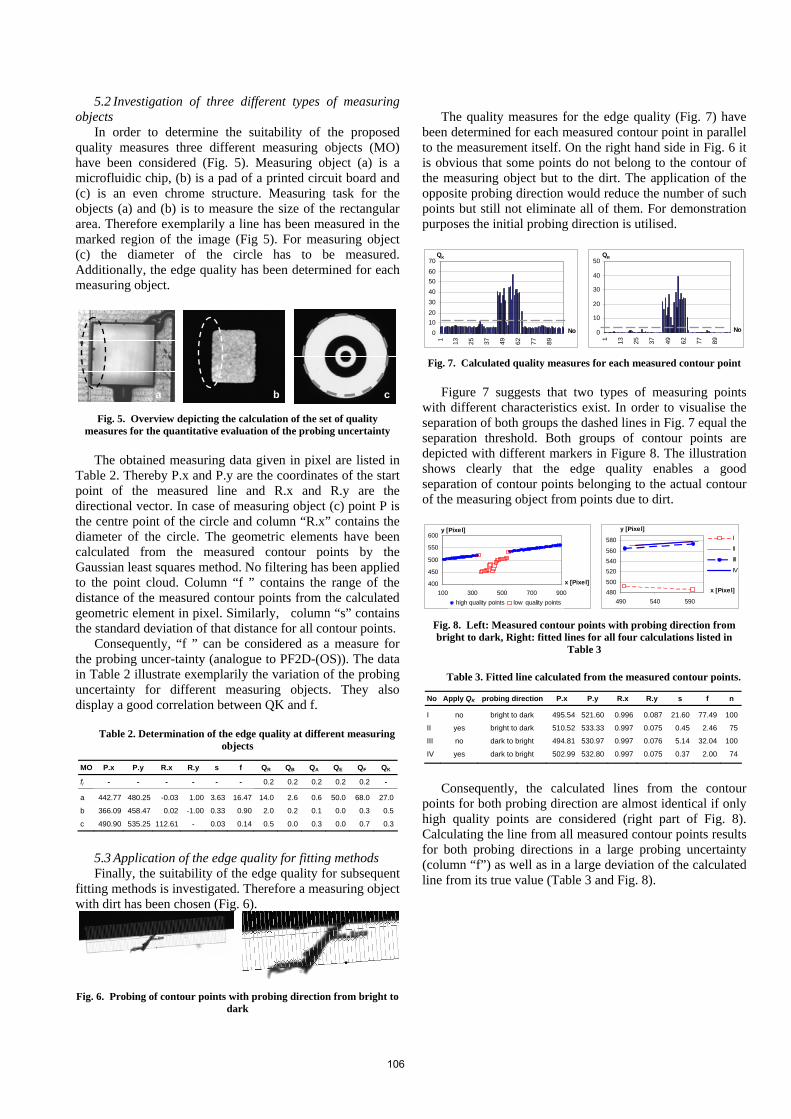
5.2 Investigation of three different types of measuring objects

In order to determine the suitability of the proposed quality measures three different measuring objects (MO) have been considered (Fig. 5). Measuring object (a) is a microfluidic chip, (b) is a pad of a printed circuit board and (c) is an even chrome structure. Measuring task for the objects (a) and (b) is to measure the size of the rectangular area. Therefore exemplarily a line has been measured in the marked region of the image (Fig 5). For measuring object (c) the diameter of the circle has to be measured. Additionally, the edge quality has been determined for each measuring object.

a cb Fig. 5. Overview depicting the calculation of the set of quality

measures for the quantitative evaluation of the probing uncertainty

The obtained measuring data given in pixel are listed in Table 2. Thereby P.x and P.y are the coordinates of the start point of the measured line and R.x and R.y are the directional vector. In case of measuring object (c) point P is the centre point of the circle and column “R.x” contains the diameter of the circle. The geometric elements have been calculated from the measured contour points by the Gaussian least squares method. No filtering has been applied to the point cloud. Column “f ” contains the range of the distance of the measured contour points from the calculated geometric element in pixel. Similarly, column “s” contains the standard deviation of that distance for all contour points.

Consequently, “f ” can be considered as a measure for the probing uncer-tainty (analogue to PF2D-(OS)). The data in Table 2 illustrate exemplarily the variation of the probing uncertainty for different measuring objects. They also display a good correlation between QK and f.

Table 2. Determination of the edge quality at different measuring

objects

MO P.x P.y R.x R.y s f QR QB QA QE QF QK

fi - - - - - - 0.2 0.2 0.2 0.2 0.2 -

a 442.77 480.25 -0.03 1.00 3.63 16.47 14.0 2.6 0.6 50.0 68.0 27.0

b 366.09 458.47 0.02 -1.00 0.33 0.90 2.0 0.2 0.1 0.0 0.3 0.5

c 490.90 535.25 112.61 - 0.03 0.14 0.5 0.0 0.3 0.0 0.7 0.3

5.3 Application of the edge quality for fitting methods Finally, the suitability of the edge quality for subsequent

fitting methods is investigated. Therefore a measuring object with dirt has been chosen (Fig. 6).

Fig. 6. Probing of contour points with probing direction from bright to

dark

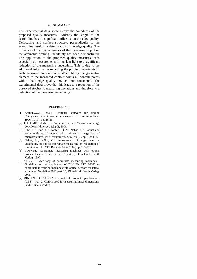
The quality measures for the edge quality (Fig. 7) have

been determined for each measured contour point in parallel to the measurement itself. On the right hand side in Fig. 6 it is obvious that some points do not belong to the contour of the measuring object but to the dirt. The application of the opposite probing direction would reduce the number of such points but still not eliminate all of them. For demonstration purposes the initial probing direction is utilised.

010203040506070

1 13 25 37 49 62 77 89

No

QK

0

10

20

30

40

50

1 13 25 37 49 62 77 89

No

QR

Fig. 7. Calculated quality measures for each measured contour point

Figure 7 suggests that two types of measuring points

with different characteristics exist. In order to visualise the separation of both groups the dashed lines in Fig. 7 equal the separation threshold. Both groups of contour points are depicted with different markers in Figure 8. The illustration shows clearly that the edge quality enables a good separation of contour points belonging to the actual contour of the measuring object from points due to dirt.

400

450

500

550

600

100 300 500 700 900

x [Pixel]

y [Pixel]

high quality points low quality points480500

520540560

580

490 540 590

x [Pixel]

I

II

III

IV

y [Pixel]

Fig. 8. Left: Measured contour points with probing direction from bright to dark, Right: fitted lines for all four calculations listed in

Table 3

Table 3. Fitted line calculated from the measured contour points.

No Apply QK probing direction P.x P.y R.x R.y s f n

I no bright to dark 495.54 521.60 0.996 0.087 21.60 77.49 100

II yes bright to dark 510.52 533.33 0.997 0.075 0.45 2.46 75

III no dark to bright 494.81 530.97 0.997 0.076 5.14 32.04 100

IV yes dark to bright 502.99 532.80 0.997 0.075 0.37 2.00 74 Consequently, the calculated lines from the contour

points for both probing direction are almost identical if only high quality points are considered (right part of Fig. 8). Calculating the line from all measured contour points results for both probing directions in a large probing uncertainty (column “f”) as well as in a large deviation of the calculated line from its true value (Table 3 and Fig. 8).

106

6. SUMMARY

The experimental data show clearly the soundness of the proposed quality measures. Evidently the length of the search line has no significant influence on the edge quality. Defocusing and surface structures perpendicular to the search line result in a deterioration of the edge quality. The influence of the characteristics of the measuring object on the attainable probing uncertainty has been demonstrated. The application of the proposed quality measures leads especially at measurements in incident light to a significant reduction of the measuring uncertainty. This is due to the additional information regarding the probing uncertainty of each measured contour point. When fitting the geometric element to the measured contour points all contour points with a bad edge quality QK are not considered. The experimental data prove that this leads to a reduction of the observed stochastic measuring deviations and therefore to a reduction of the measuring uncertainty.

REFERENCES [1] Anthony,G.T.; et.al.: Reference software for finding

Chebyshev best-fit geometric elements. In: Precision Eng., 1996, 19 (1), pp. 28-36.

[2] I++ DME Interface – Version 1.5. http://www.iacmm.org/ downloads/idmespec.1.5.pdf, 2006.

[3] Kühn, O.; Linß, G.; Töpfer, S.C.N.; Nehse, U.: Robust and accurate fitting of geometrical primitives to image data of microstructures. In: Measurement, 2007, 40 (2), pp. 129-144.

[4] Nehse, U.; Kühn, O.: Improvement of edge detection uncertainty in optical coordinate measuring by regulation of illumination. In: VDI Berichte 1694, 2002, pp. 265-275.

[5] VDI/VDE: Coordinate measuring machines with optical probes: Basics. Guideline 2617 part 6, Düsseldorf: Beuth Verlag, 1997.

[6] VDI/VDE: Accuracy of coordinate measuring machines - Guideline for the application of DIN EN ISO 10360 to coordinate measuring machines with optical sensors for lateral structures. Guideline 2617 part 6.1, Düsseldorf: Beuth Verlag, 2005.

[7] DIN EN ISO 10360-2: Geometrical Product Specifications (GPS) – Part 2: CMMs used for measuring linear dimensions, Berlin: Beuth Verlag.

107