symmetryS S

Article

A Novel Noise Suppression Channel EstimationMethod Based on Adaptive Weighted Averaging forOFDM Systems

Mingtong Zhang , Xiao Zhou * and Chengyou Wang

School of Mechanical, Electrical and Information Engineering, Shandong University, Weihai 264209, China* Correspondence: zhouxiao@sdu.edu.cn; Tel.: +86-631-568-8338

Received: 4 July 2019; Accepted: 30 July 2019; Published: 3 August 2019�����������������

Abstract: Orthogonal frequency division multiplexing (OFDM) systems have inherent symmetricproperties, such as coding and decoding, constellation mapping and demapping, inverse fastFourier transform (IFFT) and fast Fourier transform (FFT) operations corresponding to multi-carriermodulation and demodulation, and channel estimation is a necessary module to resist channel fadingin the OFDM system. However, the noise in the channel will significantly affect the accuracy ofchannel estimation, which further affects the recovery quality of the final received signals. Therefore,this paper proposes an efficient noise suppression channel estimation method for OFDM systemsbased on adaptive weighted averaging. The basic idea of the proposed method is averaging thelast few channel coefficients obtained from coarse estimation to suppress the noise effect, while theaverage frame number is adaptively adjusted by combining Doppler spread and signal-to-noiseratio (SNR) information. Meanwhile, to better combat the negative effect brought by Dopplerspread and inter-carrier interference (ICI), the proposed method introduces a weighting factor tocorrect the weighted value of each frame in the averaging process. Simulation results show that theproposed channel estimation method is effective and provides better performance compared withother conventional channel estimation methods.

Keywords: channel estimation; orthogonal frequency division multiplexing (OFDM); adaptiveweighted averaging (AWA); adaptive unweighted averaging (AUA); noise suppression

1. Introduction

Orthogonal frequency division multiplexing (OFDM) technology is widely used in moderncommunication systems for its superior performance and high spectral efficiency [1,2]. The cyclic prefix(CP) is inserted between the adjacent OFDM symbols as a guard interval (GI), which not only reducesthe inter-symbol interference (ISI) largely, but also simplifies the design of the frequency-domainequalizer [3]. For these reasons, OFDM technology has been applied to many transmission standardssuch as digital video broadcasting-terrestrial (DVB-T) and wireless local area network (WLAN) [4].In recent years, the applications of the OFDM system in underwater acoustic communication,smart grid, vehicular ad-hoc network and other fields have also received extensive attention andresearch [5–7]. The transmission reliability of OFDM systems can be further enhanced by using themultiple-input multiple-output (MIMO) technique without increasing the bandwidth [8,9]. Offsetquadrature amplitude modulation (OQAM) can also be combined with OFDM to make the systemhave lower spectral sidelobes by using the pulse shaping filters, which is a candidate technologyfor 5G communication [10,11]. In OFDM systems, channel estimation is an important module forcoherent detection and frequency-domain equalization, and the accuracy of channel estimation directlyaffects the recovery quality of the final received OFDM signals [12,13]. However, channel estimation

Symmetry 2019, 11, 997; doi:10.3390/sym11080997 www.mdpi.com/journal/symmetry

Symmetry 2019, 11, 997 2 of 20

is a challenging technology in wireless systems due to the noise effect and time variance of wirelesschannels [14,15].

There have been many researches on channel estimation in OFDM systems. In general, channelestimation methods can be divided into three categories: pilot-based channel estimation, blindchannel estimation, and semi-blind channel estimation [16]. Blind and semi-blind estimation performchannel estimation with non-pilot and few pilots, respectively, and thus have higher spectral efficiency.However, these two methods suffer from high computational complexity and are not preferred inpractice. Due to reliability and simplicity, the pilot-based channel estimation is more attractive inpractical applications [12]. Pilot-based channel estimation method estimates the channel impulseresponse (CIR) or channel frequency response (CFR) by multiplexing the known pilot sequencesinto OFDM symbols. In practice, pilot symbols are inserted in various patterns, such as block-type,comb-type, and scatter-type, to adapt to different channel environments [16]. In this paper, comb-typepilot-based channel estimation is used in OFDM systems since comb-type pilot is more robust to atime-varying channel with low to high Doppler spread.

To suppress the noise effect in the channel and obtain more accurate channel estimation results, thispaper proposes an adaptive weighted averaging (AWA)-based noise suppression channel estimationmethod. The essence of the proposed method is to average the last few channel coefficients obtainedfrom coarse estimation to suppress the noise effect, while the average frame number is adaptivelyadjusted by combining Doppler spread and signal-to-noise ratio (SNR) information. Moreover, tobetter combat the negative effect of the Doppler spread and inter-carrier interference (ICI), this paperintroduces a weighting factor to correct the weighted value of each frame in the averaging process.Simulation results show that the proposed method outperforms the conventional counterparts in termsof bit error rate (BER) and normalized mean square error (NMSE).

The remainder of this paper is organized as follows. Section 2 illustrates the related work and thesystem model is presented in Section 3. Section 4 introduces three conventional channel estimationmethods. Section 5 details the proposed AWA-based noise suppression channel estimation method.The experimental results of the proposed method are presented in Section 6. Conclusions are presentedin Section 7.

2. Related Work

There have been many conventional pilot-based channel estimation methods for OFDM systems,such as the least squares (LS) method [17], minimum mean square error (MMSE) method [18], andlinear MMSE (LMMSE) method [19,20]. The LS method is the simplest channel estimation method andhas been widely used for many years. However, the LS method ignores the noise effect, which greatlyreduces its performance [17]. The MMSE method has good estimation performance by utilizing thechannel statistic, but this method involves the inverse operation of the matrix, so its computationalcomplexity is high [18]. To reduce the computational complexity of the MMSE method, the LMMSEmethod is implemented for channel estimation in the receiver of the OFDM system [19]. However, theLMMSE method requires a priori information to calculate the channel autocorrelation matrix and itsimplementation is somewhat difficult in fast fading channels.

In recent years, researchers have proposed some new channel estimation methods. Combiningchannel soft information and Turbo decoding in an iterative way can greatly improve the accuracyof channel estimation, which can be realized by the expectation maximization (EM) algorithm orbelief propagation (BP) algorithm [21,22]. In [22], an iterative channel estimation based on a factorgraph is proposed; this method iteratively passes soft information between the channel estimation anddata decoding stages through the BP algorithm. The main disadvantage of this method is the highcomputational complexity caused by multiple iterations. Moreover, the EM algorithm is also widelyused in fast fading channel estimation [21]. Based on the strong performance of deep learning, the deeplearning-based channel estimation method is promising [23]. Different from existing OFDM receiversthat first estimate channel state information (CSI) explicitly and then recover the transmitted symbols

Symmetry 2019, 11, 997 3 of 20

using the estimated CSI, the deep learning-based method estimates CSI implicitly and recovers thetransmitted symbols directly, which has similar performance compared with the MMSE method and ismore robust than conventional methods. However, the deep learning-based method requires massiveamounts of training data samples, which is often difficult to obtain in practice [23].

The additive white Gaussian noise (AWGN) existing in wireless communication systems willsignificantly reduce the accuracy of channel estimation [24]. In recent years, researchers have putforward some noise suppression channel estimation methods. To suppress the noise effect, a threshold,which is often obtained through noise variance estimation, is applied at the LS estimation of the CIRto find the positions of the most significant taps (MSTs) [16,25]. However, a fixed threshold oftencannot distinguish the paths with smaller energy from the noise. Linear filter in time domain is also aneffective way to mitigate the noise effect, but it is not easy to determine the parameters of the linear filterin practical implementation [26]. In [27], an improved MMSE (IMMSE) channel estimation method isproposed. This method inherits the noise resistance of the MMSE method and simplifies the matrixcalculation. However, this method suffers from a loss of the partial path energy while suppressing thenoise, which decreases the estimation accuracy at high SNR scenarios. Moreover, for some widebandwireless channels, researchers have proved that the CIR often presents a sparse structure (i.e., the CIRindeed contain only a small proportion of nonzero valued coefficients) [28]. Such channels occur inradio [29] and underwater [30] communications. Some recent works exploit the channel sparsity todiscard most of the noise effect in the zero-value taps, which can significantly improve the accuracy ofthe channel estimation [28–30].

Moreover, some researchers utilize the averaging of AWGN to further suppress the noise effect,which can be combined with the above-mentioned conventional noise suppression method [16,27–30].In [31], a simple noise suppression channel estimation method based on inter-frame pilot averaging isproposed. This method can provide more accurate interpolation results because the noise power atthe pilot position is suppressed by averaging adjacent frames. Meanwhile, a similar noise reductionmethod by averaging the channel coefficients of LS estimation in two or more OFDM frames is proposedin [32,33]. These averaging methods in [31–33], which use a fixed average frame number, can beimplemented on time invariant channels and are very simple to implement in practice. However, itcannot be applied directly to dynamic channels, because the Doppler spread and the ensuing ICI indynamic channels will bring Doppler distortion in the averaging process. With the increase of theDoppler spread, the estimation accuracy of the averaging method using a fixed average frame numberdeteriorates significantly. In [34,35], a more sophisticated adaptive averaging channel estimationmethod is proposed, which adjusts the average frame number according to the Doppler spread.However, the method in [34,35] does not further consider the relationship between the averageframe number and SNR, so its performance is unstable under different SNR scenarios. On the otherhand, a weighted inter-frame averaging method for coherent optical OFDM (CO-OFDM) system isproposed in [36], which uses a weighting factor between 0 and 1 to resist the phase rotation. Inspiredby this method, this paper also introduces a weighting factor in the averaging process to resist theDoppler distortion.

To keep the performance of the averaging method optimal under different Doppler spread andSNR scenarios, this paper proposes an AWA-based noise suppression channel estimation method.As a unique feature of the averaging method, the proposed AWA method can be combined withother conventional noise suppression methods to further improve the noise suppression effect. In thispaper, the proposed method is combined with the threshold value method [25] (i.e., taking thresholdvalue estimation as the coarse estimation). This paper is novel in three points: First, it studies andanalyzes the influence of Doppler spread and SNR on the averaging method and uses the combinationof Doppler spread and SNR to adaptively determine the average frame number. Second, it introduces aweighting factor into the averaging process, which can improve the robustness against Doppler spreadand ICI. Third, it combines the proposed method with the threshold value method to further suppressthe noise in the MSTs.

Symmetry 2019, 11, 997 4 of 20

In [37], researchers committed to determine the positions of the MSTs by counting the number ofpositive and negative CIR coefficients of multiple frames, which was consistent with the goal of thethreshold value method. Therefore, the proposed method is different from the multi-frame statisticalchannel estimation method in [37]. Moreover, the proposed method can be further improved bycombining the multi-frame statistical channel estimation method. To facilitate further research, channelmodel and some simulation parameters, the same as [37], are selected in this paper.

3. System Model

A CP-OFDM system [37] with N subcarriers and utilizing the proposed channel estimationmethod, is presented in Figure 1, where NP ≤ N uniformly spaced subcarriers are used as comb-typepilots. The pilots position arranged in ascending order is denoted as P1, P2, · · · , PNP . This paperassumes that the system is perfectly synchronized and that the CP length NG should be longer than themaximum channel delay spread L (in terms of samples) to avoid the ISI problem. In the frequencyselective channel, the pilot subcarriers spacing should not exceed the coherent bandwidth, which canbe transformed to NP ≥ L [30]. Since L is unknown, this paper chooses NP ≥ NG which guarantees thatthe above constraint is respected.

Symmetry 2019, 11, x; doi: FOR PEER REVIEW www.mdpi.com/journal/symmetry

Channelestimation

X

QPSK symbol demodulation

Adaptively weighted averaging

QPSK symbol modulation

Comb-type pilots

insertionP/S

Multipath channel

S/P

IFFT ⋅⋅⋅

Cyclicprefix

addition

Serial/parallel

(S/P)

⋅⋅⋅

AWGN

FFT ⋅⋅⋅

Cyclicprefix

removal

⋅⋅⋅

Y

x

y

Input bits

Output bits

Figure 1. System model of the cyclic prefix orthogonal frequency division multiplexing (CP-OFDM) system. Abbreviations: AWGN, additive white Gaussian noise; FFT, fast Fourier transform; IFFT, inverse fast Fourier transform; QPSK, quadrature phase shift keying.

Comb-type pilot LS

Threshold denoising FFT

SNR estimation

Doppler spread estimation

Determine the average frames

adaptively

Weightedaveraging

Y ˆLSh ˆ

Th

ˆTH

fd

R

B ˆAH

ˆLSh

Figure 2. The specific processes of the proposed adaptive weighted averaging (AWA) method. Abbreviations: LS, least squares; SNR, signal-to-noise ratio.

Figure 1. System model of the cyclic prefix orthogonal frequency division multiplexing (CP-OFDM)system. Abbreviations: AWGN, additive white Gaussian noise; FFT, fast Fourier transform; IFFT,inverse fast Fourier transform; QPSK, quadrature phase shift keying.

At the receiver, the fast Fourier transform (FFT) output of the pilot symbols is expressed as [22]:

YP = XPFPh + n, (1)

where YP = [Y1, Y2, · · · , YNP ]T is the demodulated signal over the pilot subcarriers. XP is a NP ×NP

diagonal matrix containing the pilot symbols and FP is a NP × L Fourier submatrix indexed by[P1, P2, · · · , PNP ] in row and [1, 2, · · · , L] in column, obtained from the standard N×N FFT matrix F withentries Fl,m = e−j2π(l−1)(m−1)/N, where l, m = 1, 2, · · · , N. h = [h1, h2, · · · , hL]

T is the sampled equivalentCIR and n = [n1, n2, · · · , nNP ]

T is the zero-mean complex AWGN with covariance matrix σ2INP , i.e.,n ∼ CN(0, σ2INP). After FFT transformation, the estimated CSI is obtained in the channel estimationblock. The AWGN existing in the estimated channel coefficients is further suppressed in the adaptivelyweighted averaging block, which is detailed in Section 5.

4. Conventional Channel Estimation Methods

4.1. Time-Domain LS Channel Estimation

The LS method is the simplest channel estimation method for OFDM systems [17,38], and theCFR at the pilot subcarriers estimated by the LS method can be represented as:

Symmetry 2019, 11, 997 5 of 20

HP = X−1P YP = FPh + X−1

P n. (2)

Ignoring the effects of the noise item X−1P n, the CIR estimated by the LS method can be expressed as:

hLS = F+P HP = F+

P FPh + F+P X−1

P n, (3)

where F+P represents the pseudo-inverse matrix of FP, and F+

P = (FHP FP)

−1FHP = (1/NP)FH

P . FHP is the

conjugate transposition of FP. Since L is unknown, NP replaces L to guarantee that the estimated CIRlength is longer than the actual CIR length. Thus, Equation (3) can be re-written as:

hLS =1

NPFH

PSHP = hS +1

NPFH

PSX−1P n, (4)

where hS = [h1, h2, · · · , hL, 0NP−L]T is the zero expansion of the actual CIR and FPS is a NP ×NP Fourier

submatrix indexed by [P1, P2, · · · , PNP ] in row and [1, 2, · · · , NP] in column, obtained from F. Finally,the estimated CFR at all subcarriers can be obtained by applying N points FFT operation to hLS, whichavoids the interpolation in frequency domain.

4.2. IMMSE Channel Estimation

The LS channel estimation method is easy to implement in practice, but it is susceptible to thenoise effect. The IMMSE channel estimation method based on the LS method is an effective noisesuppression method [27], and the estimated de-noise CIR hIMMSE obtained from the IMMSE methodcan be expressed as:

hIMMSE(n) =hLS(n) ×

∣∣∣hLS(n)∣∣∣2

α∣∣∣hLS(n)

∣∣∣2 + (1− α)A2, 0 ≤ n ≤ NP, (5)

where A = max0≤N≤NP

(∣∣∣hLS(n)

∣∣∣) and α is the suppression factor, which is usually selected in the region

of [0.99, 1] [37]. The main disadvantage of the IMMSE method is that it suffers from a loss of thepartial path energy while suppressing the noise effect, which decreases the estimation accuracy at highSNR scenarios.

4.3. Threshold Value Channel Estimation

The threshold value method based on the LS method is also a commonly used noise suppressionchannel estimation method for OFDM systems. The essence of this method is to eliminate the noisetaps and keep the MSTs in the estimated CIR. The performance of this method is very sensitive to thethreshold, and a simple threshold proposed in [30] is expressed as:

σ2n =

1NP −NG

NP∑i=NG+1

∣∣∣hLS(i)∣∣∣2, (6)

where σ2n is the estimated variance of the noise in the LS CIR estimate. Considering NG > L, the threshold

value channel estimation results hT(n) after noise suppression can be expressed as [30]:

hT(n) =

hLS(n),∣∣∣hLS(n)

∣∣∣2 ≥ σ2n

0,∣∣∣hLS(n)

∣∣∣2 < σ2n

, 0 ≤ n ≤ NG. (7)

The disadvantage of this method is that it cannot distinguish the paths with smaller energy fromthe noise. To prevent the loss of path energy, the threshold cannot be set too high, which will reducethe noise suppression ability of the threshold value method.

Symmetry 2019, 11, 997 6 of 20

5. The Proposed Adaptive Weighted Averaging Channel Estimation Method

To improve the estimation accuracy of threshold value channel estimation method and keepsimple implementation, this paper proposes an AWA-based noise suppression channel estimationmethod. In the proposed method, the residual noise existing in the coarse channel estimation resultscan be further suppressed by averaging the estimated channel coefficients of the last few frames, whichutilizes the statistical characteristic of AWGN.

Let HT(k, n) be the CFR estimated from the threshold value method for the k-th subcarrier in then-th signal frame, and the averaging of multi-frame CFR can be expressed as [33]:

HA(k, n) =1B

n∑i=n−B+1

HT(k, i) =1B

N∑i=n−B+1

[H(k, i) + W(k, i)], 1 ≤ k ≤ N, 1 ≤ N ≤ Nt, (8)

where B is the average frame number and Nt is the total number of transmitted OFDM symbols. H(k, n)and HA(k, n) are the actual CFR and the further denoising CFR by averaging, respectively. W(k, n) isthe residual complex AWGN with covariance matrix σ2

r /IN, which exists in the threshold value channelestimation results. For the static channel, the CFR does not change with time, i.e., H(k, i) = H(k, n) fori = 1, 2, · · · , Nt. Therefore, Equation (8) can be re-written as [33]:

HA(k, n) = H(k, n) +1B

N∑i=n−B+1

W(k, i), 1 ≤ k ≤ N, 1 ≤ n ≤ Nt. (9)

According to Equation (9), the variance of the noise term is σ2r /B. Thus, theoretically, the noise

suppression effect of the averaging method increases with the increase of the average frame number inthe static channel environment.

However, there is no perfect static channel in practice. For dynamic channel, although this paperassumes that the channel is quasi-static within an OFDM symbol period, due to the influence of theDoppler spread and the ensuing ICI, the prior condition H(k, i) = H(k, n) is not satisfied and convertedto H(k, i) ≈ H(k, n) for i = 1, 2, · · · , Nt. Therefore, Equation (8) should be re-written as:

HA(k, n) = H(k, n) +1B

n∑i=n−B+1

W(k, i) + d(k, n), 1 ≤ k ≤ N, 1 ≤ n ≤ Nt, (10)

where d represents the Doppler distortion caused by the approximation due to the Doppler spread andthe ensuing ICI, and the distortion increases with the B and Doppler spread fd. To ensure that theimprovement of channel estimation accuracy brought by averaging is far greater than the negativeimpact of d, B must be adaptively adjusted by combining fd and SNR R. Meanwhile, consideringthat the correlation between two frames is inversely proportional to the distance, a weighting factorcan be introduced to correct the weighted value of each frame in the averaging process, which canbetter combat the negative effect of the Doppler spread and ICI. Therefore, this paper proposes anAWA-based noise suppression channel estimation method, which can estimate fd and R, and furtherdetermine the averaging frames adaptively. The specific processes of the proposed channel estimationmethod are shown in Figure 2.

The yellow filling blocks in Figure 2 represent the core of the proposed channel estimation method,which is the determination of the average frames and the process of weighted averaging. Next, thispaper will illustrate these two parts in detail.

5.1. Determination of the Average Frames

To adaptively determine the average frame number, fd and R must be known. Therefore, this paperuses two simple methods to estimate fd and R, respectively.

Symmetry 2019, 11, 997 7 of 20

Symmetry 2019, 11, x; doi: FOR PEER REVIEW www.mdpi.com/journal/symmetry

Channelestimation

X

QPSK symbol demodulation

Adaptively weighted averaging

QPSK symbol modulation

Comb-type pilots

insertionP/S

Multipath channel

S/P

IFFT ⋅⋅⋅

Cyclicprefix

addition

Serial/parallel

(S/P)

⋅⋅⋅

AWGN

FFT ⋅⋅⋅

Cyclicprefix

removal

⋅⋅⋅

Y

x

y

Input bits

Output bits

Figure 1. System model of the cyclic prefix orthogonal frequency division multiplexing (CP-OFDM) system. Abbreviations: AWGN, additive white Gaussian noise; FFT, fast Fourier transform; IFFT, inverse fast Fourier transform; QPSK, quadrature phase shift keying.

Comb-type pilot LS

Threshold denoising FFT

SNR estimation

Doppler spread estimation

Determine the average frames

adaptively

Weightedaveraging

Y ˆLSh ˆ

Th

ˆTH

fd

R

B ˆAH

ˆLSh

Figure 2. The specific processes of the proposed adaptive weighted averaging (AWA) method. Abbreviations: LS, least squares; SNR, signal-to-noise ratio. Figure 2. The specific processes of the proposed adaptive weighted averaging (AWA) method.Abbreviations: LS, least squares; SNR, signal-to-noise ratio.

5.1.1. Estimation of the SNR

Let Y(k, n) be the received OFDM signal in frequency domain corresponding to the k-th subcarrierin the n-th frame, and the actual received signal power S(n) for the n-th frame OFDM signal can becalculated as [39]:

S(n) =1N

N∑i=1

∣∣∣Y(i, n)∣∣∣2 = Sp(n) + Sn(n), 1 ≤ n ≤ Nt, (11)

where Sp(n) and Sn(n) represent the pure signal power and the noise power in the n-th frame OFDMsignal, respectively. Then, for the n-th frame OFDM signal, its received SNR in decibel form can beexpressed as:

R(n) = 10 log10

[Sp(n)/Sn(n)

]= 10 log10[(S(n) − Sn(n))/Sn(n)], 1 ≤ n ≤ Nt. (12)

Therefore, the estimation of the SNR can be realized only by the noise power of the receivedsignal. According to Equation (1), the noise n contained in the received pilot signal YP is the zero-meancomplex AWGN with covariance matrix σ2INP . Therefore, the noise power of the n-th frame OFDMsignal is Sn(n) = σ2.

Meanwhile, according to Equation (4), the noise item of the CIR obtained by the LS method is alsothe zero-mean complex AWGN, and its covariance matrix σ2

nINP can be expressed as:

σ2nINP =

σ2

N2P

FHPSX−1

P INP(FHPSX−1

P )H=σ2

N2P

1∣∣∣X(Pi)∣∣∣2 FH

PSFPSINP , (13)

where X(Pi) represents the quadrature phase shift keying (QPSK) signal at the pilot position, and thus∣∣∣X(Pi)∣∣∣2 = 2. Meanwhile, considering FH

PSFPS = NPINP , Equation (13) can be re-written as:

σ2nINP = σ2/(2NP) × INP . (14)

Therefore, Sn(n) = σ2 = 2NPσ2n, and σ2

n can be estimated by Equation (6). Finally, the estimationof the received SNR in decibel form can be expressed as:

R(n) = 10 · log10

[(S(n) − 2NPσ

2n)/(2NPσ

2n)

], 1 ≤ n ≤ Nt. (15)

5.1.2. Estimation of the Doppler Spread

The estimation of fd in this paper is based on the fact that the autocorrelation function of thereceived pilot symbols in time domain can be expressed as a Bessel function [34], i.e.,

r(∆i) = J0(2π fd∆iT), (16)

Symmetry 2019, 11, 997 8 of 20

where J0(·) is the first type of zero-order Bessel function and ∆i is the difference in the OFDM symbolnumber. T is the OFDM symbol duration. Then search for the first negative value of r(∆i) and letthat ∆i be z. The first zero crossing point z0 of r(∆i) can be determined by linear interpolation asfollows [34]:

z0 =r(z)

r(z− 1) − r(z)+ z, (17)

where the autocorrelation r(·) is estimated as follows:

r(∆i) =1

Nt − |∆i|

Nt−|∆i|∑n=1

(yn × y∗n+∆i), (18)

where yn represents the received n-th frame OFDM signal in the time domain. The first zero crossingpoint of J0(x) is x = 2.405 [34]. That is, r(∆i) becomes zero for the first time when 2π fd∆iT = 2.405.Thus, using the estimated zero crossing point z0, the Doppler spread can be estimated as [34]:

fd =2.4052πTz0

. (19)

5.1.3. Determine the Average Frames Adaptively

In the proposed channel estimation method, B is a key parameter for the dynamic channel, and itshould be adaptively adjusted by combining R and fd which are obtained from Equations (15) and (19),respectively. As the duration of each OFDM frame is T, the duration of the averaging frames is equalto TB = B× T.

To make the distortion d in Equation (10) small, there should be a strong correlation between theframes used for averaging (i.e., the channel is almost flat within the time interval TB). Considering thechannel coherence time TC can be expressed as [40]:

TC =9

16π fd≈

0.179fd

, (20)

and the coherence time TC should be much larger than TB, which can be expressed as:

TB =TC

γ, (21)

where γ� 1 is a correction factor. Combining Equations (20) and (21), B can be determined as:

B = floor(0.179

γ fdT), (22)

where floor(·) is a rounding down function.In Equation (22), γ is a key and unknown parameter that determines the average frame number.

At different SNR levels, the distortion that can be allowed is different (i.e., the larger the SNR is, themore obvious the negative effect of the distortion will be, and the stronger the correlation betweenthe frames used for averaging should be). Meanwhile, the distortion increases with the increase of fd.Therefore, γ should be related to R and fd.

Since floor(·) is used in Equation (22), the optimal value of γ corresponding to different R and fdis not limited to a strictly accurate number, but a fluctuation range, which relaxes the requirementfor the estimation accuracy of R and fd. This can be expressed as Figure 3, whereby the fluctuationrange of the optimal value of γ corresponding to different R and fd are indicated by the vertical bars.Noted that the optimal value of γ simulated in Figure 3 (solid line) is obtained by searching step bystep with step length 0.1 according to Equation (22). It can be observed that there is an approximate

Symmetry 2019, 11, 997 9 of 20

exponential function relationship between γ and R, and the exponential curve shifts up and downwith the increase and decrease of fd. Therefore, after data fitting, this paper uses Equation (23) to fitthe exponential function relationship, and it is fine-tuned by fd. Thus γ can be expressed as:

γ = ρeR14

[1 +

13

log2(40fd)

], (23)

where ρ is a parameter related to the weight of the averaging frames and it is selected as ρ = 2 for theproposed AWA method.

Symmetry 2019, 11, x FOR PEER REVIEW 9 of 21

Since floor( ) is used in Equation (22), the optimal value of γ corresponding to different R

and fd is not limited to a strictly accurate number, but a fluctuation range, which relaxes the

requirement for the estimation accuracy of R and fd . This can be expressed as Figure 3, whereby

the fluctuation range of the optimal value of γ corresponding to different R and fd are

indicated by the vertical bars. Noted that the optimal value of γ simulated in Figure 3 (solid line)

is obtained by searching step by step with step length 0.1 according to Equation (22). It can be

observed that there is an approximate exponential function relationship between γ and R , and

the exponential curve shifts up and down with the increase and decrease of fd . Therefore, after data

fitting, this paper uses Equation (23) to fit the exponential function relationship, and it is fine-tuned

by fd . Thus γ can be expressed as:

( )142

d

1 40e 1 log ,

3

R

γ ρf

= +

(23)

where ρ is a parameter related to the weight of the averaging frames and it is selected as =ρ 2 for

the proposed AWA method.

(a) (b)

Figure 3. The optimal value of γ corresponding to different R and fd selected by simulation or

calculation of Equation (23) obtained from 44 10 trail runs: (a) 20 and 60 Hz; (b) 40 and 80 Hz.

In Figure 3, the legend of “Calculated” means the value of γ calculated from Equation (23). It

can be seen that the Equation (23) can be acceptable for [ ]R 0,25 dB and low to medium Doppler

spread conditions according to simulation. Therefore, combining Equations (22) and (23), the average

frame number B can be determined as:

ˆ ˆ.log ( ) .

ˆ

− =

R fB

ρf T

d142

d

0 537floor e

320 (24)

5.2. The Process of Weighted Averaging

Through a large number of simulation experiments, if the weight of each frame for averaging is

always one (i.e., unweighted), the parameter ρ in Equation (23) should be =ρ 2.6 . The adaptive

unweighted averaging (AUA) of multi-frame channel coefficients can be expressed as:

ˆ ˆ( ) ( )M

M = − +

i n M

k n k i k N, n NH H1

1

U T t11

1, = , , 1 1 , (25)

Figure 3. The optimal value of γ corresponding to different R and fd selected by simulation orcalculation of Equation (23) obtained from 4× 104 trail runs: (a) 20 and 60 Hz; (b) 40 and 80 Hz.

In Figure 3, the legend of “Calculated” means the value of γ calculated from Equation (23). It canbe seen that the Equation (23) can be acceptable for R ∈ [0, 25]dB and low to medium Doppler spreadconditions according to simulation. Therefore, combining Equations (22) and (23), the average framenumber B can be determined as:

B = floor

0.537

ρ fdTe−

R14 log2(

fd320

)

. (24)

5.2. The Process of Weighted Averaging

Through a large number of simulation experiments, if the weight of each frame for averagingis always one (i.e., unweighted), the parameter ρ in Equation (23) should be ρ = 2.6. The adaptiveunweighted averaging (AUA) of multi-frame channel coefficients can be expressed as:

HU(k, n) =1

M1

M1∑i=n−M1+1

HT(k, i), 1 ≤ k ≤ N, 1 ≤ n ≤ Nt, (25)

where M1 = min[B1, n], B1 is obtained by putting ρ = 2.6 into Equation (24).Considering that the correlation between two frames is inversely proportional to the distance,

a weighting factor can be introduced to correct the weighted value of each frame in the averagingprocess. The estimated CFR in the AWA channel estimation method can be expressed as:

HW(k, n) = (1/M2∑i=1

i)M2∑i=1

[iHT(k, n−M2 + i)], 1 ≤ k ≤ N, 1 ≤ n ≤ Nt, (26)

Symmetry 2019, 11, 997 10 of 20

where M2 = min[B2, n], B2 is obtained by putting ρ = 2.0 into Equation (24). It can be observed fromEquation (26) that the frame used for averaging has a greater weight if it is closer to the current frame,which can better combat the negative effect of the Doppler spread and ICI.

In the AWA channel estimation method, since the channel is almost flat within the time intervalTB = B× T, the distortion brought by the Doppler spread and ICI can be neglected, and Equation (26)can be re-written as:

HW(k, n) = H(k, n) +2

M2(M2 + 1)

M2∑i=1

[iW(k, n−M2 + i)], 1 ≤ k ≤ N, 1 ≤ n ≤ Nt. (27)

Because W ∼ CN(0, σ2r IN), the variance of the noise term in Equation (27) can be expressed as:

σ2W = σ2

r

1/M2∑i=1

i

2 M2∑

i=1

i2 =σ2

r (4M2 + 2)3M2(M2 + 1)

. (28)

Since B2 � Nt in practice, the assumption M2 = B2 can be accepted and the noise suppressionratio of the AWA method is approximately equal to (4B2 + 2)/[3B2(B2 + 1)].

In the same way, the noise suppression ratio of the AUA method can be obtained from Equation (25),and it is approximately equal to 1/B1. The theoretical average frame number B and noise suppressionratio of the AWA and AUA methods under different SNR and Doppler spread are presented in Figure 4.

In Figure 4a, with the increase of the SNR and Doppler spread, the theoretical average framenumber of the AWA and AUA methods is all decreasing. Under the same condition, the AWA methodhas a more average frame number than the AUA method. Therefore, although the noise suppressioneffect of the AWA method is slightly worse under the same average frame number, its final noisesuppression effect is stronger than the AUA method, which can be seen from Figure 4b. At the noisesuppression ratio of 0.1, 0.2, and 0.3, the AWA method has about 0.6 dB, 2.5 dB, and 3.8 dB SNR gainscompared with AUA method for fd equal to 10 Hz, 20 Hz, and 60 Hz, respectively. It can be seen thatthe SNR gains increase with the increase of Doppler spread, which is because the AWA method canbetter combat the negative effect of the Doppler spread and ICI.Symmetry 2019, 11, x FOR PEER REVIEW 11 of 21

(a)

(b)

Figure 4. The theoretical performance value of the AWA and adaptive unweighted averaging (AUA)

methods under different R and fd : (a) average frame number B ; (b) noise suppression ratio.

According to Equation (27), the proposed method mainly increases the addition operation and

storage resources, so its computational complexity is in the same order as the threshold value method.

Therefore, the proposed method is convenient for hardware implementation in practice.

6. Simulation Results and Performance Analysis

In this section, the simulation experiments are presented to demonstrate the performance of the

proposed AWA-based noise suppression channel estimation method. The simulation is performed in

static and dynamic multipath environments, respectively. The multipath channel models are China

digital television (DTV) Test 1st (CDT1), CDT6, Brazil A, Brazil B, and Brazil D, where CDT1 and

CDT6 channels are from the field tests for digital terrestrial television broadcasting (DTTB) in China

and Brazil A, Brazil B, and Brazil D [19] channels are from the field tests for DTTB in Brazil [33]. These

five channels are typical multipath broadcasting channel models, and all belong to the Rayleigh

fading channel. CDT1 and Brazil A channels have slight frequency selectivity; CDT6, Brazil B, and

Brazil D channels have stronger frequency selectivity.

The profiles for the Brazil A, Brazil B, and Brazil D channel models are shown in Table 1. The

profiles for the CDT1 and CDT6 channel models are shown in Table 2. The main simulation

parameters for the OFDM system are presented in Table 3.

Table 1. Profiles for Brazil A, Brazil B, and Brazil D channel models.

Tap Brazil A Brazil B Brazil D

Delay (μs) Power (dB) Delay (μs) Power (dB) Delay (μs) Power (dB)

1 0 0 0 0 0 −0.10

2 0.15 −13.80 0.30 −12 0.48 −3.90

3 2.22 −16.20 3.50 −4 2.07 −2.60

4 3.05 −14.90 4.40 −7 2.90 −1.30

5 5.86 −13.60 9.50 −15 5.71 0

6 5.93 −16.40 12.70 −22 5.78 −2.80

Table 2. Profiles for China digital television (DTV) Test 1st (CDT1) and CDT6 channel models.

Tap CDT1 CDT6

Delay (μs) Power (dB) Delay (μs) Power (dB)

1 0 0 0 0

2 −1.8 −20 −18 −10

3 0.15 −20 −1.80 −20

Figure 4. The theoretical performance value of the AWA and adaptive unweighted averaging (AUA)methods under different R and fd: (a) average frame number B; (b) noise suppression ratio.

According to Equation (27), the proposed method mainly increases the addition operation andstorage resources, so its computational complexity is in the same order as the threshold value method.Therefore, the proposed method is convenient for hardware implementation in practice.

Symmetry 2019, 11, 997 11 of 20

6. Simulation Results and Performance Analysis

In this section, the simulation experiments are presented to demonstrate the performance of theproposed AWA-based noise suppression channel estimation method. The simulation is performed instatic and dynamic multipath environments, respectively. The multipath channel models are Chinadigital television (DTV) Test 1st (CDT1), CDT6, Brazil A, Brazil B, and Brazil D, where CDT1 and CDT6channels are from the field tests for digital terrestrial television broadcasting (DTTB) in China andBrazil A, Brazil B, and Brazil D [19] channels are from the field tests for DTTB in Brazil [33]. These fivechannels are typical multipath broadcasting channel models, and all belong to the Rayleigh fadingchannel. CDT1 and Brazil A channels have slight frequency selectivity; CDT6, Brazil B, and Brazil Dchannels have stronger frequency selectivity.

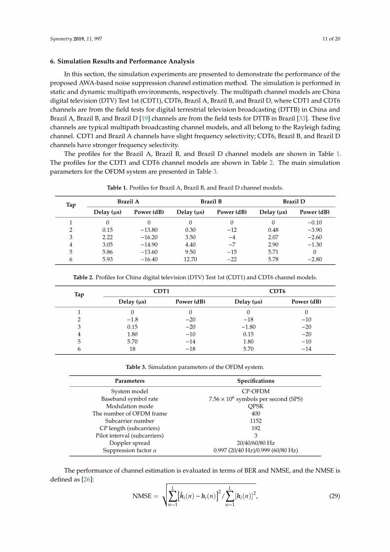
The profiles for the Brazil A, Brazil B, and Brazil D channel models are shown in Table 1.The profiles for the CDT1 and CDT6 channel models are shown in Table 2. The main simulationparameters for the OFDM system are presented in Table 3.

Table 1. Profiles for Brazil A, Brazil B, and Brazil D channel models.

Tap Brazil A Brazil B Brazil D

Delay (µs) Power (dB) Delay (µs) Power (dB) Delay (µs) Power (dB)

1 0 0 0 0 0 −0.102 0.15 −13.80 0.30 −12 0.48 −3.903 2.22 −16.20 3.50 −4 2.07 −2.604 3.05 −14.90 4.40 −7 2.90 −1.305 5.86 −13.60 9.50 −15 5.71 06 5.93 −16.40 12.70 −22 5.78 −2.80

Table 2. Profiles for China digital television (DTV) Test 1st (CDT1) and CDT6 channel models.

Tap CDT1 CDT6

Delay (µs) Power (dB) Delay (µs) Power (dB)

1 0 0 0 02 −1.8 −20 −18 −103 0.15 −20 −1.80 −204 1.80 −10 0.15 −205 5.70 −14 1.80 −106 18 −18 5.70 −14

Table 3. Simulation parameters of the OFDM system.

Parameters Specifications

System model CP-OFDMBaseband symbol rate 7.56 × 106 symbols per second (SPS)

Modulation mode QPSKThe number of OFDM frame 400

Subcarrier number 1152CP length (subcarriers) 192

Pilot interval (subcarriers) 3Doppler spread 20/40/60/80 Hz

Suppression factor α 0.997 (20/40 Hz)/0.999 (60/80 Hz)

The performance of channel estimation is evaluated in terms of BER and NMSE, and the NMSE isdefined as [26]:

NMSE =

√√√ L∑n=1

[hi(n) − hi(n)

]2/

L∑n=1

[hi(n)]2, (29)

Symmetry 2019, 11, 997 12 of 20

where hi(n) and hi(n) represent the estimated CIR by various channel estimation methods and realCIR in the i-th frame, respectively. BER reflects the overall performance of the wireless communicationsystem, NMSE reflects the estimation accuracy of various channel estimation methods. They are thetwo most commonly used indicators in the field of channel estimation.

The conventional LS, threshold value, IMMSE, and the proposed AWA and AUA channelestimation methods are presented in the CP-OFDM system. Moreover, an ideal channel estimation(ICE) method is given in the simulation results, which is the channel estimation with the known channelcoefficients, as a reference. In the CP-OFDM system, the number of total subcarriers is 1152, and the CPoccupies 192 subcarriers. Therefore, the total number of actual application subcarriers including pilotand data is N =1152− 192 = 960, where NP= N/4 = 240 comb-type pilot subcarriers are employed.For both pilots and data, the symbols are drawn from a QPSK constellation. The baseband symbol rateof the CP-OFDM system is 7.56× 106 symbols per second and the duration of each OFDM frame isT = 1152/7.56× 10−6 s = 152.38µs. In dynamic multipath environments, Doppler spread is chosento be 20 Hz, 40 Hz, 60 Hz, and 80 Hz, respectively. According to [27], the suppression factor α inthe IMMSE method is 0.997 for a Doppler spread equal to 20 Hz or 40 Hz and 0.999 for a Dopplerspread equal to 60 Hz or 80 Hz, which can suppress the AWGN effectively with a smaller loss of thepartial path energy. For a better study of the performance of the proposed method, neither interleavingmethods nor any channel coding techniques are used.

6.1. The Performance in Static Channel

The NMSE performance of fixed and adaptive multi-frame averaging methods under a staticCDT1 channel is shown in Figure 5. The BER and NMSE performance of LS, threshold value, IMMSE,and the proposed channel estimation methods under static CDT6 channel are shown in Figures 6and 7, respectively.

Symmetry 2019, 11, x FOR PEER REVIEW 13 of 21

Figure 5. Normalized mean square error (NMSE) performance of fixed and adaptive multi-frame

averaging method under static China digital television (DTV) Test 1st (CDT1) channel.

As can be seen from Figure 5, the NMSE of the six channel estimation curves all decreases with

the increase of the SNR. For fixed multi-frame averaging method, the NMSE decreases with the

increase of the average frame number. In Figure 5, the AUA method has the best NMSE performance,

which is slightly better than the AWA method. The reason is that there is no Doppler spread in the

static channel, and the advantage of weighted averaging against the negative effect of the Doppler

spread and the ensuing ICI cannot be reflected. At the NMSE of − 25 10 , the proposed AUA method

can provide about 0.9 dB and 11.2 dB SNR gains compared with the AWA and fixed 8-frame

averaging methods, respectively. Moreover, the gaps of the SNR gain among fixed 8-frame, 6-frame,

4-frame, and 2-frame averaging methods is about 1.2 dB, 1.7 dB, and 3.1 dB at the NMSE of − 25 10 ,

respectively. Therefore, under the static CDT1 channel, the proposed adaptive averaging method is

much better than the fixed averaging method.

Figure 5. Normalized mean square error (NMSE) performance of fixed and adaptive multi-frameaveraging method under static China digital television (DTV) Test 1st (CDT1) channel.

As can be seen from Figure 5, the NMSE of the six channel estimation curves all decreases with theincrease of the SNR. For fixed multi-frame averaging method, the NMSE decreases with the increaseof the average frame number. In Figure 5, the AUA method has the best NMSE performance, whichis slightly better than the AWA method. The reason is that there is no Doppler spread in the staticchannel, and the advantage of weighted averaging against the negative effect of the Doppler spread

Symmetry 2019, 11, 997 13 of 20

and the ensuing ICI cannot be reflected. At the NMSE of 5 × 10−2, the proposed AUA method canprovide about 0.9 dB and 11.2 dB SNR gains compared with the AWA and fixed 8-frame averagingmethods, respectively. Moreover, the gaps of the SNR gain among fixed 8-frame, 6-frame, 4-frame, and2-frame averaging methods is about 1.2 dB, 1.7 dB, and 3.1 dB at the NMSE of 5× 10−2, respectively.Therefore, under the static CDT1 channel, the proposed adaptive averaging method is much betterthan the fixed averaging method.

Symmetry 2019, 11, x FOR PEER REVIEW 13 of 21

Figure 5. Normalized mean square error (NMSE) performance of fixed and adaptive multi-frame

averaging method under static China digital television (DTV) Test 1st (CDT1) channel.

As can be seen from Figure 5, the NMSE of the six channel estimation curves all decreases with

the increase of the SNR. For fixed multi-frame averaging method, the NMSE decreases with the

increase of the average frame number. In Figure 5, the AUA method has the best NMSE performance,

which is slightly better than the AWA method. The reason is that there is no Doppler spread in the

static channel, and the advantage of weighted averaging against the negative effect of the Doppler

spread and the ensuing ICI cannot be reflected. At the NMSE of − 25 10 , the proposed AUA method

can provide about 0.9 dB and 11.2 dB SNR gains compared with the AWA and fixed 8-frame

averaging methods, respectively. Moreover, the gaps of the SNR gain among fixed 8-frame, 6-frame,

4-frame, and 2-frame averaging methods is about 1.2 dB, 1.7 dB, and 3.1 dB at the NMSE of − 25 10 ,

respectively. Therefore, under the static CDT1 channel, the proposed adaptive averaging method is

much better than the fixed averaging method.

Figure 6. Bit error rate (BER) performance under static CDT6 channel. Abbreviations: ICE, idealchannel estimation; IMMSE, improved minimum mean square error.

Symmetry 2019, 11, x FOR PEER REVIEW 14 of 21

Figure 6. Bit error rate (BER) performance under static CDT6 channel. Abbreviations: ICE, ideal

channel estimation; IMMSE, improved minimum mean square error.

Figure 7. NMSE performance under static CDT6 channel.

In Figure 6, the proposed AUA and AWA methods have almost the same BER performance, and

both of them can improve the channel estimation performance in the overall SNR range similar to the

ICE method. The reason is that there is no distortion caused by averaging under the static channel.

Compared with the IMMSE, threshold value, and LS methods, the proposed AWA method has about

0.3 dB, 1.6 dB, and 2.6 dB SNR gains at the BER of −310 . It can be seen that AWGN is the main factor

affecting the accuracy of channel estimation, and the noise effect can be significantly suppressed by

the proposed AWA method under the static CDT6 channel.

In Figure 7, the proposed AUA method has the best NMSE performance, and it can provide

about 0.9 dB and 10.6 dB SNR gains compared with the proposed AWA method and IMMSE method

at the target NMSE of − 25 10 . Meanwhile, the gaps of the SNR gain among the IMMSE, threshold

value, and LS methods are about 8.1 dB and 1.1 dB at the NMSE of − 25 10 , respectively. This is

because the average frame number of the AWA method is the same as that of the AUA method under

the static channel, and the noise suppression ability of the AWA method is slightly worse under the

same average frame number, which can be seen from Equation (28). Although the NMSE

performance of the AUA method is slightly better than that of the AWA method in the static CDT6

channel, the BER performance of these two methods is almost identical, which can be seen from

Figure 6. Therefore, in the static scenarios, the weight has little influence on the proposed adaptive

averaging method.

6.2. The Performance in Dynamic Channel

The NMSE performance of fixed and adaptive multi-frame averaging methods under Brazil A

channel with Doppler spread 40 Hz is shown in Figure 8. The BER and NMSE performance of the LS,

threshold value, IMMSE, and the proposed channel estimation methods under Brazil A channel with

Doppler spread 20 Hz are shown in Figures 9 and 10, respectively.

Figure 7. NMSE performance under static CDT6 channel.

In Figure 6, the proposed AUA and AWA methods have almost the same BER performance, andboth of them can improve the channel estimation performance in the overall SNR range similar to theICE method. The reason is that there is no distortion caused by averaging under the static channel.Compared with the IMMSE, threshold value, and LS methods, the proposed AWA method has about

Symmetry 2019, 11, 997 14 of 20

0.3 dB, 1.6 dB, and 2.6 dB SNR gains at the BER of 10−3. It can be seen that AWGN is the main factoraffecting the accuracy of channel estimation, and the noise effect can be significantly suppressed by theproposed AWA method under the static CDT6 channel.

In Figure 7, the proposed AUA method has the best NMSE performance, and it can provide about0.9 dB and 10.6 dB SNR gains compared with the proposed AWA method and IMMSE method at thetarget NMSE of 5× 10−2. Meanwhile, the gaps of the SNR gain among the IMMSE, threshold value,and LS methods are about 8.1 dB and 1.1 dB at the NMSE of 5 × 10−2, respectively. This is becausethe average frame number of the AWA method is the same as that of the AUA method under thestatic channel, and the noise suppression ability of the AWA method is slightly worse under the sameaverage frame number, which can be seen from Equation (28). Although the NMSE performance ofthe AUA method is slightly better than that of the AWA method in the static CDT6 channel, the BERperformance of these two methods is almost identical, which can be seen from Figure 6. Therefore,in the static scenarios, the weight has little influence on the proposed adaptive averaging method.

6.2. The Performance in Dynamic Channel

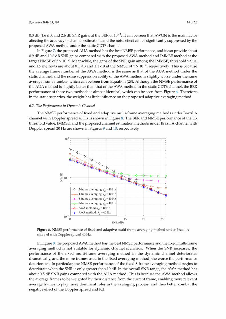
The NMSE performance of fixed and adaptive multi-frame averaging methods under Brazil Achannel with Doppler spread 40 Hz is shown in Figure 8. The BER and NMSE performance of the LS,threshold value, IMMSE, and the proposed channel estimation methods under Brazil A channel withDoppler spread 20 Hz are shown in Figures 9 and 10, respectively.

Symmetry 2019, 11, x FOR PEER REVIEW 15 of 21

Figure 8. NMSE performance of fixed and adaptive multi-frame averaging method under Brazil A

channel with Doppler spread 40 Hz.

In Figure 8, the proposed AWA method has the best NMSE performance and the fixed multi-

frame averaging method is not suitable for dynamic channel scenarios. When the SNR increases, the

performance of the fixed multi-frame averaging method in the dynamic channel deteriorates

dramatically, and the more frames used in the fixed averaging method, the worse the performance

deteriorates. In particular, the NMSE performance of the fixed 8-frame averaging method begins to

deteriorate when the SNR is only greater than 10 dB. In the overall SNR range, the AWA method has

about 0.5 dB SNR gains compared with the AUA method. This is because the AWA method allows

the average frames to be weighted by their distance from the current frame, enabling more relevant

average frames to play more dominant roles in the averaging process, and thus better combat the

negative effect of the Doppler spread and ICI.

Figure 9. BER performance under Brazil A channel with Doppler spread 20 Hz.

Figure 8. NMSE performance of fixed and adaptive multi-frame averaging method under Brazil Achannel with Doppler spread 40 Hz.

In Figure 8, the proposed AWA method has the best NMSE performance and the fixed multi-frameaveraging method is not suitable for dynamic channel scenarios. When the SNR increases, theperformance of the fixed multi-frame averaging method in the dynamic channel deterioratesdramatically, and the more frames used in the fixed averaging method, the worse the performancedeteriorates. In particular, the NMSE performance of the fixed 8-frame averaging method begins todeteriorate when the SNR is only greater than 10 dB. In the overall SNR range, the AWA method hasabout 0.5 dB SNR gains compared with the AUA method. This is because the AWA method allowsthe average frames to be weighted by their distance from the current frame, enabling more relevantaverage frames to play more dominant roles in the averaging process, and thus better combat thenegative effect of the Doppler spread and ICI.

Symmetry 2019, 11, 997 15 of 20

Symmetry 2019, 11, x FOR PEER REVIEW 15 of 21

Figure 8. NMSE performance of fixed and adaptive multi-frame averaging method under Brazil A

channel with Doppler spread 40 Hz.

In Figure 8, the proposed AWA method has the best NMSE performance and the fixed multi-

frame averaging method is not suitable for dynamic channel scenarios. When the SNR increases, the

performance of the fixed multi-frame averaging method in the dynamic channel deteriorates

dramatically, and the more frames used in the fixed averaging method, the worse the performance

deteriorates. In particular, the NMSE performance of the fixed 8-frame averaging method begins to

deteriorate when the SNR is only greater than 10 dB. In the overall SNR range, the AWA method has

about 0.5 dB SNR gains compared with the AUA method. This is because the AWA method allows

the average frames to be weighted by their distance from the current frame, enabling more relevant

average frames to play more dominant roles in the averaging process, and thus better combat the

negative effect of the Doppler spread and ICI.

Figure 9. BER performance under Brazil A channel with Doppler spread 20 Hz. Figure 9. BER performance under Brazil A channel with Doppler spread 20 Hz.Symmetry 2019, 11, x FOR PEER REVIEW 16 of 21

Figure 10. NMSE performance under Brazil A channel with Doppler spread 20 Hz.

As shown in Figures 9 and 10, the proposed AWA method provides better NMSE performance

as well as system BER than the other channel estimation methods except the ICE method. For example,

in Figure 9, at the BER of − 35 10 , compared with the ICE method, the proposed AWA method has

about 0.8 dB SNR degradation, compared with the AUA, IMMSE, threshold value, and LS methods,

the proposed AWA method has about 0.1 dB, 0.6 dB, 1.4 dB, and 2.1 dB SNR gains, respectively. In

Figure 10, at the NMSE of −110 , compared with the AUA, IMMSE, threshold value, and LS methods,

the proposed AWA method has about 0.5 dB, 1.8 dB, 7.4 dB, and 9.3 dB SNR gains, respectively. Thus,

the proposed adaptive averaging-based noise suppression channel estimation method works well

under Brazil A channel with Doppler spread 20 Hz, and its performance can be further improved by

introducing weighting factor to combat the distortion caused by Doppler spread and ICI.

The BER and NMSE performance of the LS, threshold value, IMMSE, and the proposed channel

estimation methods under Brazil B channel with Doppler spread 60 Hz are shown in Figures 11 and

12, respectively.

Figure 10. NMSE performance under Brazil A channel with Doppler spread 20 Hz.

As shown in Figures 9 and 10, the proposed AWA method provides better NMSE performance aswell as system BER than the other channel estimation methods except the ICE method. For example,in Figure 9, at the BER of 5 × 10−3, compared with the ICE method, the proposed AWA method hasabout 0.8 dB SNR degradation, compared with the AUA, IMMSE, threshold value, and LS methods,the proposed AWA method has about 0.1 dB, 0.6 dB, 1.4 dB, and 2.1 dB SNR gains, respectively.In Figure 10, at the NMSE of 10−1, compared with the AUA, IMMSE, threshold value, and LS methods,the proposed AWA method has about 0.5 dB, 1.8 dB, 7.4 dB, and 9.3 dB SNR gains, respectively. Thus,the proposed adaptive averaging-based noise suppression channel estimation method works wellunder Brazil A channel with Doppler spread 20 Hz, and its performance can be further improved byintroducing weighting factor to combat the distortion caused by Doppler spread and ICI.

Symmetry 2019, 11, 997 16 of 20

The BER and NMSE performance of the LS, threshold value, IMMSE, and the proposed channelestimation methods under Brazil B channel with Doppler spread 60 Hz are shown in Figures 11and 12, respectively.

Symmetry 2019, 11, x FOR PEER REVIEW 16 of 21

Figure 10. NMSE performance under Brazil A channel with Doppler spread 20 Hz.

As shown in Figures 9 and 10, the proposed AWA method provides better NMSE performance

as well as system BER than the other channel estimation methods except the ICE method. For example,

in Figure 9, at the BER of − 35 10 , compared with the ICE method, the proposed AWA method has

about 0.8 dB SNR degradation, compared with the AUA, IMMSE, threshold value, and LS methods,

the proposed AWA method has about 0.1 dB, 0.6 dB, 1.4 dB, and 2.1 dB SNR gains, respectively. In

Figure 10, at the NMSE of −110 , compared with the AUA, IMMSE, threshold value, and LS methods,

the proposed AWA method has about 0.5 dB, 1.8 dB, 7.4 dB, and 9.3 dB SNR gains, respectively. Thus,

the proposed adaptive averaging-based noise suppression channel estimation method works well

under Brazil A channel with Doppler spread 20 Hz, and its performance can be further improved by

introducing weighting factor to combat the distortion caused by Doppler spread and ICI.

The BER and NMSE performance of the LS, threshold value, IMMSE, and the proposed channel

estimation methods under Brazil B channel with Doppler spread 60 Hz are shown in Figures 11 and

12, respectively.

Figure 11. BER performance under Brazil B channel with Doppler spread 60 Hz.

Symmetry 2019, 11, x FOR PEER REVIEW 17 of 21

Figure 11. BER performance under Brazil B channel with Doppler spread 60 Hz.

Figure 12. NMSE performance under Brazil B channel with Doppler spread 60 Hz.

By comparing Figures 9 and 10 with Figures 11 and 12, it can be seen that the performance under

Brazil B channel is worse than Brazil A channel, which is because Brazil B channel has stronger

frequency selectivity and Doppler spread than Brazil A channel. However, the proposed AWA

method still has the best performance among the six channel estimation methods except the ICE

method. In Figure 11, the proposed AWA method can provide about 0.2 dB, 0.3 dB, 1.1 dB, and 1.8

dB SNR gains, and has about 1.1 dB SNR degradation, compared with the AUA, IMMSE, threshold

value, LS, and ICE methods at the BER of −210 , respectively. Therefore, with the increase of Doppler

spread, the AWA method has more obvious advantages over the AUA method. In Figure 12, the

IMMSE method has bad NMSE performance when the SNR is higher than 18 dB. This is because the

IMMSE method suffers from a loss of the partial path energy while suppressing the noise effect. At

the NMSE of −110 , the proposed AWA method has about 0.5 dB, 1.5 dB, 4.1 dB, and 5.6 dB SNR gains

compared with the AUA, IMMSE, threshold value, and LS methods, respectively. It can be seen that

the proposed AWA method effectively suppresses the residual noise in the threshold value channel

estimation and greatly improves the accuracy of channel estimation.

The BER and NMSE performance of the LS, threshold value, IMMSE, and the proposed channel

estimation methods under Brazil D channel with Doppler spread 80 Hz are shown in Figures 13 and

14, respectively.

Figure 12. NMSE performance under Brazil B channel with Doppler spread 60 Hz.

By comparing Figures 9 and 10 with Figures 11 and 12, it can be seen that the performanceunder Brazil B channel is worse than Brazil A channel, which is because Brazil B channel has strongerfrequency selectivity and Doppler spread than Brazil A channel. However, the proposed AWA methodstill has the best performance among the six channel estimation methods except the ICE method.In Figure 11, the proposed AWA method can provide about 0.2 dB, 0.3 dB, 1.1 dB, and 1.8 dB SNRgains, and has about 1.1 dB SNR degradation, compared with the AUA, IMMSE, threshold value, LS,and ICE methods at the BER of 10−2, respectively. Therefore, with the increase of Doppler spread, theAWA method has more obvious advantages over the AUA method. In Figure 12, the IMMSE method

Symmetry 2019, 11, 997 17 of 20

has bad NMSE performance when the SNR is higher than 18 dB. This is because the IMMSE methodsuffers from a loss of the partial path energy while suppressing the noise effect. At the NMSE of 10−1,the proposed AWA method has about 0.5 dB, 1.5 dB, 4.1 dB, and 5.6 dB SNR gains compared with theAUA, IMMSE, threshold value, and LS methods, respectively. It can be seen that the proposed AWAmethod effectively suppresses the residual noise in the threshold value channel estimation and greatlyimproves the accuracy of channel estimation.

The BER and NMSE performance of the LS, threshold value, IMMSE, and the proposed channelestimation methods under Brazil D channel with Doppler spread 80 Hz are shown in Figures 13and 14, respectively.Symmetry 2019, 11, x FOR PEER REVIEW 18 of 21

Figure 13. BER performance under Brazil D channel with Doppler spread 80 Hz.

Figure 14. NMSE performance under Brazil D channel with Doppler spread 80 Hz.

In Figures 13 and 14, the IMMSE method has bad BER and NMSE performance when the SNR

is higher than 20 dB, and the proposed AWA method has the best BER and NMSE performance when

the SNR is lower than 30 dB. In Figure 13, the proposed AWA method can provide about 0.1 dB, 0.1

dB, 0.9 dB, and 1.7 dB SNR gains, and has about 1.0 dB SNR degradation, compared with the AUA,

IMMSE, threshold value, LS, and ICE methods at the BER of −210 , respectively. In Figure 14, at the

NMSE of −110 , the proposed AWA method has about 0.8 dB, 0.9 dB, 3.7 dB, and 5.4 dB SNR gains

compared with the AUA, IMMSE, threshold value, and LS methods, respectively. However, when

the SNR is greater than 30 dB, the performance of the proposed AWA method is no longer optimal.

This is because the noise effect is small in the high SNR and Doppler spread scenarios, and the

channel distortion brought by the averaging becomes significant.

7. Conclusions

Figure 13. BER performance under Brazil D channel with Doppler spread 80 Hz.

Symmetry 2019, 11, x FOR PEER REVIEW 18 of 21

Figure 13. BER performance under Brazil D channel with Doppler spread 80 Hz.

Figure 14. NMSE performance under Brazil D channel with Doppler spread 80 Hz.

In Figures 13 and 14, the IMMSE method has bad BER and NMSE performance when the SNR

is higher than 20 dB, and the proposed AWA method has the best BER and NMSE performance when

the SNR is lower than 30 dB. In Figure 13, the proposed AWA method can provide about 0.1 dB, 0.1

dB, 0.9 dB, and 1.7 dB SNR gains, and has about 1.0 dB SNR degradation, compared with the AUA,

IMMSE, threshold value, LS, and ICE methods at the BER of −210 , respectively. In Figure 14, at the

NMSE of −110 , the proposed AWA method has about 0.8 dB, 0.9 dB, 3.7 dB, and 5.4 dB SNR gains

compared with the AUA, IMMSE, threshold value, and LS methods, respectively. However, when

the SNR is greater than 30 dB, the performance of the proposed AWA method is no longer optimal.

This is because the noise effect is small in the high SNR and Doppler spread scenarios, and the

channel distortion brought by the averaging becomes significant.

7. Conclusions

Figure 14. NMSE performance under Brazil D channel with Doppler spread 80 Hz.

In Figures 13 and 14, the IMMSE method has bad BER and NMSE performance when the SNR ishigher than 20 dB, and the proposed AWA method has the best BER and NMSE performance when theSNR is lower than 30 dB. In Figure 13, the proposed AWA method can provide about 0.1 dB, 0.1 dB,

Symmetry 2019, 11, 997 18 of 20

0.9 dB, and 1.7 dB SNR gains, and has about 1.0 dB SNR degradation, compared with the AUA, IMMSE,threshold value, LS, and ICE methods at the BER of 10−2, respectively. In Figure 14, at the NMSE of10−1, the proposed AWA method has about 0.8 dB, 0.9 dB, 3.7 dB, and 5.4 dB SNR gains compared withthe AUA, IMMSE, threshold value, and LS methods, respectively. However, when the SNR is greaterthan 30 dB, the performance of the proposed AWA method is no longer optimal. This is because thenoise effect is small in the high SNR and Doppler spread scenarios, and the channel distortion broughtby the averaging becomes significant.

7. Conclusions

In this paper, we studied the multi-frame averaging scheme in the frequency domain for channelestimation and proposed an adaptive weighted averaging-based noise suppression channel estimationmethod. Combined with the Doppler spread and SNR information, the proposed method can adaptivelyselect the average frame number, so it can adapt to the dynamic channel. Moreover, the introductionof weights improves the robustness of the proposed method to the Doppler distortion. Specially,the proposed method can be combined with other conventional noise suppression methods, such asthe threshold value method in this paper, to further eliminate the residual noise effect existing in thechannel estimation results, and significantly improve the channel estimation accuracy. Simulationresults show that the proposed channel estimation method can provide a good performance understatic and dynamic multipath channels. Yet under the dynamic channels with very large Dopplerspread and SNR, the performance of the proposed adaptive weighted averaging method needs to befurther improved.

Compared with the conventional LS, IMMSE, and threshold value methods, the proposed adaptiveweighted averaging-based noise suppression channel estimation method has the best BER and NMSEperformance. Meanwhile, the proposed method has the same order computational complexity as thethreshold value method, so it can be easily implemented in practice and has broad market prospectsthat can be applied in MIMO technique, OQAM technique, and cognitive radio technique.

Author Contributions: M.Z. and X.Z. conceived the algorithm and designed the experiments; M.Z. performedthe experiments; X.Z. and C.W. analyzed the results; M.Z. drafted the manuscript; M.Z., X.Z., and C.W. revised themanuscript. All authors read and approved the final manuscript.

Funding: This work was supported by the National Natural Science Foundation of China (Grant No. 61702303)and the Shandong Provincial Natural Science Foundation, China (Grant No. ZR2017MF020).

Acknowledgments: The authors gratefully acknowledge the technical assistance of DL850E ScopeCorderadministrated by Xiaoli Wang.

Conflicts of Interest: The authors declare no conflicts of interest.

References

1. Liu, Y.S.; Tan, Z.H.; Hu, H.J.; Cimini, L.J.; Li, G.Y. Channel estimation for OFDM. IEEE Commun. Surv. Tutor.2014, 16, 1891–1908. [CrossRef]

2. Uwaechia, A.N.; Mahyuddin, N.M. Spectrum-efficient distributed compressed sensing based channelestimation for OFDM systems over doubly selective channels. IEEE Access 2019, 7, 35072–35088. [CrossRef]

3. Xiong, X.; Jiang, B.; Gao, X.Q.; You, X.H. DFT-based channel estimator for OFDM systems with leakageestimation. IEEE Commun. Lett. 2013, 17, 1592–1595. [CrossRef]

4. Chin, W. Nondata-aided Doppler frequency estimation for OFDM systems over doubly selective fadingchannels. IEEE Trans. Commun. 2018, 66, 4211–4221. [CrossRef]

5. Panayirci, E.; Altabbaa, M.T.; Uysal, M.; Poor, H.V. Sparse channel estimation for OFDM-based underwateracoustic systems in Rician fading with a new OMP-MAP algorithm. IEEE Trans. Signal Process. 2019, 67,1550–1565. [CrossRef]

6. Wu, L.B.; Wang, J.; Zeadally, S.; He, D.B. Anonymous and efficient message authentication scheme for smartgrid. Secur. Commun. Netw. 2019, 2019, 4836016. [CrossRef]

Symmetry 2019, 11, 997 19 of 20

7. Tan, H.W.; Choi, D.; Kim, P.; Pan, S.; Chung, I. Secure certificateless authentication and road messagedissemination protocol in VANETs. Wirel. Commun. Mob. Comput. 2018, 2018, 7978027. [CrossRef]

8. Jeon, H.J.; Song, H.K.; Serpedin, E. Walsh coded training signal aided time domain channel estimation forMIMO-OFDM systems. IEEE Trans. Commun. 2008, 56, 1430–1433. [CrossRef]

9. Ding, W.B.; Yang, F.; Dai, W.; Song, J. Time-frequency joint sparse channel estimation for MIMO-OFDMsystems. IEEE Commun. Lett. 2015, 19, 58–61. [CrossRef]

10. Fuhrwerk, M.; Moghaddamnia, S.; Peissig, J. Scattered pilot-based channel estimation for channel adaptiveFBMC-OQAM systems. IEEE Trans. Wirel. Commun. 2017, 16, 1687–1702. [CrossRef]

11. Kong, D.J.; Qu, D.M.; Jiang, T. Time domain channel estimation for OQAM-OFDM systems: Algorithms andperformance bounds. IEEE Trans. Signal Process. 2014, 62, 322–330. [CrossRef]

12. Li, Y. Pilot-symbol-aided channel estimation for OFDM in wireless systems. IEEE Trans. Veh. Technol. 2000,49, 1207–1215. [CrossRef]

13. Jellali, Z.; Atallah, L.N. Time varying sparse channel estimation by MSE optimization in OFDM systems. InProceedings of the IEEE 77th Vehicular Technology Conference, Dresden, Germany, 2–5 June 2013; pp. 1–5.

14. Uwaechia, A.N.; Mahyuddin, N.M. Collaborative framework of algorithms for sparse channel estimation inOFDM systems. J. Commun. Netw. 2018, 20, 9–19.

15. Wang, L.; Hanzo, L. Dispensing with channel estimation: Differentially modulated cooperative wirelesscommunications. IEEE Commun. Surv. Tutor. 2012, 14, 836–857. [CrossRef]

16. Tang, R.G.; Zhou, X.; Wang, C.Y. A Haar wavelet decision feedback channel estimation method in OFDMsystems. Appl. Sci. 2018, 8, 877. [CrossRef]

17. Beek, J.J.; Edfors, O.; Sandell, M.; Wilson, S.K.; Borjesson, P.O. On channel estimation in OFDM systems.In Proceedings of the IEEE 45th Vehicular Technology Conference, Chicago, IL, USA, 25–28 July 1995;pp. 815–819.

18. Sutar, M.B.; Patil, V.S. LS and MMSE estimation with different fading channels for OFDM system.In Proceedings of the 1st International Conference of Electronics, Communication and Aerospace Technology,Coimbatore, India, 20–22 April 2017; pp. 740–745.

19. Tang, R.G.; Zhou, X.; Wang, C.Y. A novel low rank LMMSE channel estimation method in OFDM systems. InProceedings of the IEEE 17th International Conference on Communication Technology, Chengdu, China,27–30 October 2017; pp. 249–253.

20. Edfors, O.; Sandell, M.; Beek, J.J.; Wilson, S.K.; Borjesson, P.O. OFDM channel estimation by singular valuedecomposition. IEEE Trans. Commun. 1998, 46, 931–939. [CrossRef]

21. Schniter, P. A message-passing receiver for BICM-OFDM over unknown clustered-sparse channels. IEEE J.Sel. Top. Signal Process. 2011, 5, 1462–1474. [CrossRef]

22. Hansen, T.L.; Jørgensen, P.B.; Badiu, M.A.; Fleury, B.H. An iterative receiver for OFDM with sparsity-basedparametric channel estimation. IEEE Trans. Signal Process. 2018, 66, 5454–5469. [CrossRef]

23. Ye, H.; Li, G.Y.; Juang, B.H. Power of deep learning for channel estimation and signal detection in OFDMsystems. IEEE Wirel. Commun. Lett. 2018, 7, 114–117. [CrossRef]

24. Mezghani, A.; Swindlehurst, A.L. Blind estimation of sparse broadband massive MIMO channels with idealand one-bit ADCs. IEEE Trans. Signal Process. 2018, 66, 2972–2983. [CrossRef]

25. Lee, Y.S.; Shin, H.C.; Kim, H.N. Channel estimation based on a time-domain threshold for OFDM systems.IEEE Trans. Broadcast. 2009, 55, 656–662.

26. Zhou, X.; Ye, Z.; Liu, X.X.; Wang, C.Y. Channel estimation based on linear filtering least square in OFDMsystems. J. Commun. 2016, 11, 1005–1011. [CrossRef]

27. Zhou, X.; Yang, F.; Song, J. A novel noise suppression method in channel estimation. IEICE Trans. Fund.Electron. Commun. Comput. Sci. 2011, E94–A, 2027–2030. [CrossRef]

28. Jellali, Z.; Atallah, L.N. Fast fading channel estimation by Kalman filtering and CIR support tracking. IEEETrans. Broadcast. 2017, 63, 635–643. [CrossRef]

29. Dziwoki, G.; Izydorczyk, J. Iterative identification of sparse mobile channels for TDS-OFDM systems. IEEETrans. Broadcast. 2016, 62, 384–397. [CrossRef]

30. Shi, X.L.; Yang, Y.X. Adaptive sparse channel estimation based on RLS for underwater acoustic OFDMsystems. In Proceedings of the 6th International Conference on Instrumentation and Measurement, Computer,Communication and Control, Harbin, China, 21–23 July 2016; pp. 266–269.

Symmetry 2019, 11, 997 20 of 20

31. Zettas, S.; Kasampalis, S.L.; Lazaridis, P.; Zaharis, Z.D.; Cosmas, J. Channel estimation for OFDM systemsbased on a time domain pilot averaging scheme. In Proceedings of the 16th International Symposium onWireless Personal Multimedia Communications, Atlantic City, NJ, USA, 24–27 June 2013; pp. 1–6.

32. Lee, Y.S.; Kim, H.N.; Park, S.L.; Lee, S.L. Noise reduction for channel estimation based on pilot-blockaveraging in DVB-T receivers. IEEE Trans. Consum. Electron. 2006, 52, 51–58.

33. Lee, Y.S.; Kim, H.N.; Son, K.S. Noise-robust channel estimation for DVB-T fixed receptions. IEEE Trans.Consum. Electron. 2007, 53, 27–32.

34. Zettas, S.; Lazaridis, P.I.; Zaharis, Z.D.; Kasampalis, S.; Cosmas, J. Adaptive averaging channel estimationfor DVB-T2 using Doppler shift information. In Proceedings of the 9th IEEE International Symposium onBroadband Multimedia Systems and Broadcasting, Beijing, China, 25–27 June 2014; pp. 1–6.

35. Zettas, S.; Lazaridis, P.I.; Zaharis, Z.D.; Kasampalis, S.; Cosmas, J. A pilot aided averaging channel estimatorfor DVB-T2. In Proceedings of the 8th IEEE International Symposium on Broadband Multimedia Systemsand Broadcasting, London, UK, 5–7 June 2013; pp. 1–8.

36. Zhao, H.; Li, J.H.; Zhu, P.K.; Zhang, C.; Liu, Y.; Zhao, Y.P.; He, Y.Q.; Chen, Z.Y. Weighted inter-frameaveraging-based channel estimation for CO-OFDM system. IEEE Photonics J. 2013, 5, 7902807. [CrossRef]

37. Zhou, X.; Wang, C.Y.; Tang, R.G.; Zhang, M.T. Channel estimation based on statistical frames and confidencelevel in OFDM systems. Appl. Sci. 2018, 8, 1607. [CrossRef]

38. Zhou, X.; Yang, F.; Song, J. Novel transmit diversity scheme for TDS-OFDM system with frequency-shiftm-sequence padding. IEEE Trans. Broadcast. 2012, 58, 317–324. [CrossRef]

39. He, P.; Li, Z.X.; Wang, X. A low-complexity SNR estimation algorithm and channel estimation methodfor OFDM systems. In Proceedings of the 4th IEEE International Conference on Information Science andTechnology, Shenzhen, China, 26–28 April 2014; pp. 698–701.

40. Rappaport, T.S. Wireless Communications: Principles and Practice, 2nd ed.; Publishing House of ElectronicsIndustry: Beijing, China, 2012; pp. 139–141.

© 2019 by the authors. Licensee MDPI, Basel, Switzerland. This article is an open accessarticle distributed under the terms and conditions of the Creative Commons Attribution(CC BY) license (http://creativecommons.org/licenses/by/4.0/).