Embed Size (px)
Citation preview

A C T A U N I V E R S I T A T I S L O D Z I E N S I S FOLIA OECONOMICA 295, 2013
[59]
Władysław Milo*, Dominika Bogusz**, Mariusz Górajski***, Magdalena Ulrichs****
NOTES ON SOME OPTIMAL MONETARY POLICY
RULES: THE CASE OF POLAND1
Abstract. The paper contains results concerning theoretical and practical utility of a simple optimal control model describing monetary policy rules. Solving this model enables to find useful forms of optimal monetary rules for the two policy scenarios. They were derived for the given form of linear VAR(s) state model describing the time evolution of deviations of logarithmic values of GDP growth rates around its HP-filtered potential counterparts, empirical CPI inflation rates around NBP-target rates and expected inflation rates around long-term trend expectations, as well as, for the two forms of -cost functionals expressing two paths of optimal NBP target interest. Numerical values of these rates, obtained for Polish quarterly data, were the base both for calculating corresponding to them values of target inflation rates, GDP-growth rates, and also for making some remarks about their behaviour in comparison to their empirical counterparts.
Keywords: interest rates, central banks and their policies, VAR models, optimal rules of monetary policy.
1. Introduction
The content of this chapter belongs to very narrow section of macroeconomic foundations of theory of monetary policy of central banks. Readers interested in the complex subject of theoretical and practical problems of making monetary policy should refer to Woodford (2003), Solow and Taylor (1998).
The aim of the chapter is to present remarks on Polish monetary policy rules, and to assess the degree of their optimality. We derive the optimal rule of making monetary policy, where the policy instrument (control variable) is the deviation of log-interest rate around its trend value and the aim of central bank is to minimize the cost functional defined as the weighted variance of state and control variables. We assume more realistically that the time horizon is finite. Our empirical optimal monetary policy model for the Polish economy uses VAR-state submodel estimated on the quarterly data for the period 1995–2011.
* Full professor, Department of Econometrics, University of Łódź, Poland. **Assistant professor, Department of Econometrics, University of Łódź, Poland. ***Assistant professor, Department of Econometrics, University of Łódź, Poland. ****Assistant professor, Department of Econometrics, University of Łódź, Poland. 1Supported by the Department of Econometrics, University of Łódz.
Władysław Milo, Dominika Bogusz, Mariusz Górajski, Magdalena Ulrichs 60
On the basis of the estimated VAR model the two optimal paths of interest rates were found (Scenario 1, 2 in Section 5). Optimal solution is derived in discrete time using stochastic linear-quadratic regulator with time delays. The optimal paths are compared with the empirical trajectories and some empirical conclusions are formulated.
The chapter is organized as follows. In Section 2, we present a brief literature overview of theory and practice of monetary policy. Section 3 defines optimal monetary policy model and presents its optimal solution. Next, in Section 4, we present estimation of VAR model for the Polish economy. Section 5 contains an analysis of optimal solutions. Our conclusions are stated in Section 6.
2. Framework The possibility of choice and evaluation of monetary policy in the context of
the implementation of inflation targeting strategy is very important from the point of view of making monetary policy. However, modelling the monetary policy reaction function is difficult, because it combines some theoretical aspects and the aspects that are not subject to formal description. A number of authors have proposed simple rules for monetary policy in which they assumed that the policy instrument (e.g. short-term interest rate) is a function of some indicator variables that describe the deviations of the state of economy from some desired levels. The survey of the literature on these rules can be found in Clarida et al. (1999), McCallum (1998). These rules can be divided into two main categories – the rules relating to the purpose (control of the exchange rate, money supply, as well as control the level of inflation), and the rules relating to instruments (e.g. interest rate). Most often used in contemporary research interest rate rule is based on the equation of Taylor (1993) – the so-called Taylor rule. According to this rule interest rate linearly responds to the output gap and deviation of the annual inflation from a desired target. In some literature, the emphasis is put on the estimation of the parameters of the central bank's reaction functions without empirical determination of an optimal response. Empirical studies indicate that this rule well illustrates changes in interest rates (Baranowski 2008, 2011, Clarida et al. 1998, Judd and Rudebusch 1998, Mehra 1999, Taylor 1993, 1999, Urbańska 2002, Woodford 2001), but does not always give accurate answers to what level they should be set (Sławiński 2011). In many papers, including Ball (1997), Clarida et al. (1999), Orphanides and Wilcox (1996), Rotemberg and Woodford (1998), Svensson (1997) and Woodford 1999), authors have shown some empirical examples of interest rate rules and compare them with the optimal behaviour of central bank.
Urbańska (2002), Baranowski (2011) showed some estimations of Taylor-type rules for Poland. The results show that Polish monetary authorities do not respond to output gap, strongly respond to inflation and pay high attention to
Notes on Some Optimal Monetary Policy Rules: the Case of Poland 61
interest rate smoothing, which provides some rationale for the loss function as in Scenario 1 (see Section 5.1). How much the Taylor policy instrument is effective in determining the difference between the real inflation rate and its central bank target value and the level of output gap for developed, developing and undeveloped economies is a hard question. It is possible that the effectiveness is lowering quite quickly under low interest rate, as it has been observed in Japan from the 90’s of XX c. till now.
A common approach to modelling monetary policy is based on the estimated multiple-equation model of the monetary transmission mechanism (Mishkin 1996), taking into account the impact of central bank monetary policy on inflation and the real economy through the channel of interest rates, inflation expectations and the exchange rate. Models of this type are commonly used by central banks (in Poland see for example: Wróbel, Pawłowska 2002, Łyziak 2002, Postek 2011, Kłos et al. 2004, Łyziak et al. 2012, Demchuk et al. 2012, Brzoza-Brzezina 2011, Sławiński 2011).
In many empirical models (e.g. Batini and Haldane 1999, Rudebusch, Svensson 1999, McCallum and Nelson 2000, Sack 2000, Svensson 2000, Polito, Wickens 2012) the main objective of the central bank, which acts in infinite horizon, is usually taken into account by including the cost functional based on the exchange between the distance of inflation from its target and output gap. In this way the stochastic optimal control models are created. These classes of models due to the fact that they allow the determination of optimal interest rates are often used in research. In Gali (2007), Rotemberg and Woodford (1999) and Woodford (2003) authors show that this type of objective function can be derived from micro foundations.
3. Optimal monetary policy model The main objective of monetary policy in Poland is to maintain price
stability. Since 1999 the direct inflation targeting has been implemented into Polish monetary policy. The Monetary Policy Council sets the inflation target and then regulates the interest rates in order to achieve the established inflation target. Since 2004 National Bank of Poland has pursued a continuous inflation target at the level of 2.5% with a possible fluctuations band of +/– 1 percentage point. However, in 2011 the Monetary Policy Council specified inflation target more precisely – bringing the inflation as close as possible to its target constant level 2.5%. The NBP-monetary policy tries to influence basic nominal short-term money market rates in order to affect demand for loans and deposits and therefore to control the total consumers demand through the targets of inflation rates. Therefore, it is rational to assume the short inflation-target horizon.
Władysław Milo, Dominika Bogusz, Mariusz Górajski, Magdalena Ulrichs 62
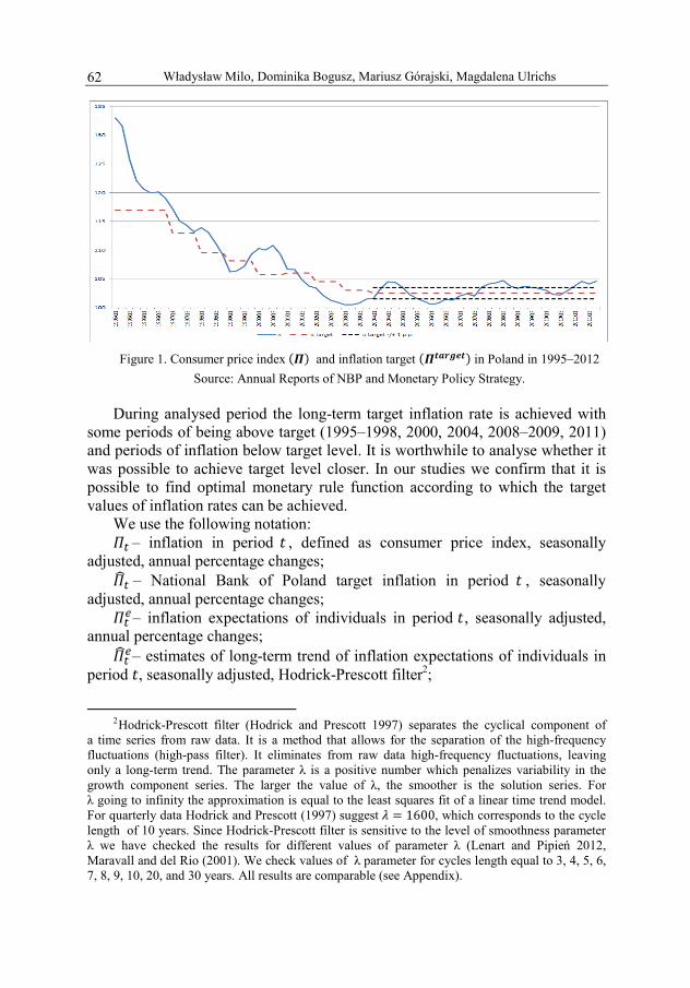
Figure 1. Consumer price index and inflation target in Poland in 1995–2012
Source: Annual Reports of NBP and Monetary Policy Strategy. During analysed period the long-term target inflation rate is achieved with
some periods of being above target (1995–1998, 2000, 2004, 2008–2009, 2011) and periods of inflation below target level. It is worthwhile to analyse whether it was possible to achieve target level closer. In our studies we confirm that it is possible to find optimal monetary rule function according to which the target values of inflation rates can be achieved.
We use the following notation: – inflation in period , defined as consumer price index, seasonally
adjusted, annual percentage changes; – National Bank of Poland target inflation in period , seasonally
adjusted, annual percentage changes; – inflation expectations of individuals in period , seasonally adjusted,
annual percentage changes; – estimates of long-term trend of inflation expectations of individuals in
period , seasonally adjusted, Hodrick-Prescott filter2;
2Hodrick-Prescott filter (Hodrick and Prescott 1997) separates the cyclical component of
a time series from raw data. It is a method that allows for the separation of the high-frequency fluctuations (high-pass filter). It eliminates from raw data high-frequency fluctuations, leaving only a long-term trend. The parameter λ is a positive number which penalizes variability in the growth component series. The larger the value of λ, the smoother is the solution series. For λ going to infinity the approximation is equal to the least squares fit of a linear time trend model. For quarterly data Hodrick and Prescott (1997) suggest 1600, which corresponds to the cycle length of 10 years. Since Hodrick-Prescott filter is sensitive to the level of smoothness parameter λ we have checked the results for different values of parameter λ (Lenart and Pipień 2012, Maravall and del Rio (2001). We check values of λ parameter for cycles length equal to 3, 4, 5, 6, 7, 8, 9, 10, 20, and 30 years. All results are comparable (see Appendix).
Notes on Some Optimal Monetary Policy Rules: the Case of Poland 63
– real in period – seasonally adjusted, at constant prices of 2005; – potential in period , seasonally adjusted, Hodrick-Prescott filter;
– interest rate in period , WIBOR1M, seasonally adjusted; – estimates of long-term trend of interest rate in period , seasonally
adjusted, Hodrick-Prescott filter; We write , , … to denote logarithms of Π , , … . Let , , and , , be column vectors of state
variables and their trend-like or targets form, respectively. The economy fluctuations , ,
from the expected target state is described by (1). The only tool used to influence the economy state is to make it fluctuated around “target” by the use of control (steering) , being the deviation of log-interest rate around its trend value . Thus, we are interested in time evolution of percentage deviation of inflation, inflation expectations, GDP and interest rate from their long-run trends or in the case of inflation its target values. For simplicity, the model is described by vector autoregressive (VAR) specification with exogenous variable.
Let 1 denote the number of lags and 1 is a time horizon. Consider VAR equation for with exogenous variable :
Ξ
, , … , are given,
, 1,2, … , (1)
where: – vector of shocks in period ; for 1,2, … , , are 3 3 , 3 1 and 3 3 matrices of parameters, respectively.
Random vectors Ξ , … Ξ are assumed to be stochastically independent with mean vector equals to 0,0,0 and with identity covariance operators .
We assume that the cost functional is of the form:
,
1
1
– 1
, ,
(2)
Władysław Milo, Dominika Bogusz, Mariusz Górajski, Magdalena Ulrichs 64
where 1 0 0
0 00 0 0
, , , 0,1 , and , is inner
product in . The weight 1 represents the attitude to financial stability. Thus, by (2)
the grater 1 the more stable behavior of interest rate is. The weights , 1 are responsible for closeness to the target inflation and minimizing the output gap, respectively.
A pair , is called a -optimal if it satisfies equation
(1) and the inequality
, , (3)
holds for all pairs , of stochastic processes evolving according
to (1). Next, we analyse existence and uniqueness of -optimal pair. Therefore, one
may observe that the system (1)–((2) can be rewritten equivalently into the following one
Ξ
, , … , is given,, 1,2, … , (4)
and
, , (5)
where
Y , Y , … , Y and 0
…… 0
0…0
…0
… 0… …0
,
0,
0, 0
0 0
are fixed unknown non-random parameters matrices. We call (4)–(5) the Markovian representation of the problem (1)–((2). If is an invertible matrix, then by Theorem 5.1.1 in Zabczyk (1996) the system (4)–(5) possesses

Notes on Some Optimal Monetary Policy Rules: the Case of Poland 65
the unique -optimal solution , . The -optimal control
is then given by the formula:
(6)
for 0,1, … , 1, where is symmetric, nonnegative matrix which is the solution to the Riccati equation:
, (7)
for 0,1, … , 1. It is worth mentioning that the optimal control for the system (4)–(5) is independent of the noise (see Corollary 5.1.1 in Zabczyk 1996).
The -optimal state is the solution of the equation
Ξ ,
(8)
for 1, … , .
Hence -optimal state is given by
Ξ ,
(9)
for 1, … , and , … , , , … , . The formula (6) is called -optimal monetary policy rule. The parameter
matrix in (6) depends due to on time, the horizon , and by on weights , conforming the cost functional as well as on the parameter matrices from the state equation (1). By the properties of the Riccati equation (7) the sequence of tends to constant matrix M as goes to infinity. Thus only in infinite horizon we obtain time-invariant optimal monetary rule.
4. Empirical results In our empirical verification a version of the model is used to
describe time evolution of macroeconomic variables . The dependencies in the model are closely related to the neokeynesian DSGE hybrid model of
Władysław Milo, Dominika Bogusz, Mariusz Górajski, Magdalena Ulrichs 66
monetary policy (cf. Clarida et al. 1999). It is seen that according to the dynamic IS equation – the real output gap depends on real interest rates and expected real output gap, i.e.:
1 ,
where denotes the logarithmic HP-trend rational expectations. The inflation rate is modelled by the hybrid New Keynesian Phillips curve and depends on deviations of expected inflation rate around its HP-trend values, lagged inflation rate and real output gap:
,
where is AR(1) cost-push shock. The welfare losses experienced by the representative household (cost functional) are, up to a second order approximation, equal to
where is the weight of output gap fluctuation (relative). Our VAR system consists of three endogenous variables: ,
, and exogenous control variable and is represented by (4):
Ξ , 1,2, … , ,
where: Y , Y , … , Y and , , , matrix of parameters connected with endogenous variables , matrix of parameters connected with exogenous instrument variable , covariance matrix of shocks.
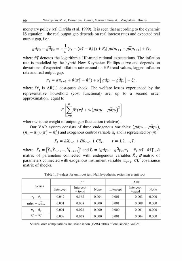
Table 1. P-values for unit root test. Null hypothesis: series has a unit root
Series PP ADF
Intercept Intercept + trend
None Intercept Intercept +trend
None
0.047 0.162 0.004 0.001 0.003 0.000
0.001 0.008 0.000 0.001 0.008 0.000
0.001 0.028 0.000 0.000 0.001 0.000
0.008 0.038 0.000 0.001 0.004 0.000
Source: own computations and MacKinnon (1996) tables of one-sided p-values.
Notes on Some Optimal Monetary Policy Rules: the Case of Poland 67
The parameters , , are estimated with the use of quarterly data for the Polish economy. The sample period covers years 1995q1–2011q4. All the data used were seasonally adjusted. Augmented Dickey-Fuller (ADF) and Phillips-Perron (PP) tests confirm stationarity of all variables.
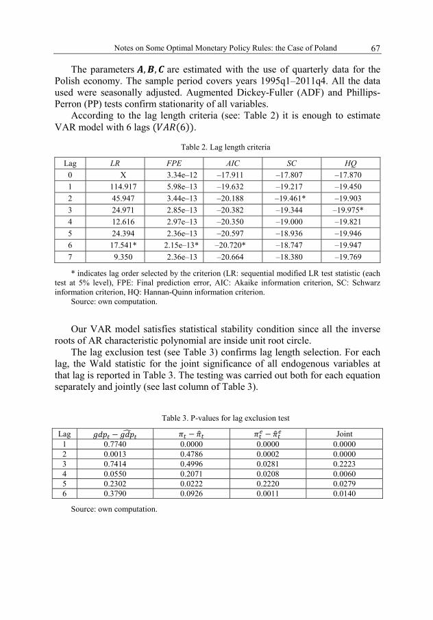
According to the lag length criteria (see: Table 2) it is enough to estimate VAR model with 6 lags 6 .
Table 2. Lag length criteria
Lag LR FPE AIC SC HQ
0 X 3.34e–12 –17.911 –17.807 –17.870
1 114.917 5.98e–13 –19.632 –19.217 –19.450
2 45.947 3.44e–13 –20.188 –19.461* –19.903
3 24.971 2.85e–13 –20.382 –19.344 –19.975*
4 12.616 2.97e–13 –20.350 –19.000 –19.821
5 24.394 2.36e–13 –20.597 –18.936 –19.946
6 17.541* 2.15e–13* –20.720* –18.747 –19.947
7 9.350 2.36e–13 –20.664 –18.380 –19.769
* indicates lag order selected by the criterion (LR: sequential modified LR test statistic (each test at 5% level), FPE: Final prediction error, AIC: Akaike information criterion, SC: Schwarz information criterion, HQ: Hannan-Quinn information criterion.
Source: own computation.
Our VAR model satisfies statistical stability condition since all the inverse roots of AR characteristic polynomial are inside unit root circle.
The lag exclusion test (see Table 3) confirms lag length selection. For each lag, the Wald statistic for the joint significance of all endogenous variables at that lag is reported in Table 3. The testing was carried out both for each equation separately and jointly (see last column of Table 3).
Table 3. P-values for lag exclusion test
Lag Joint 1 0.7740 0.0000 0.0000 0.0000 2 0.0013 0.4786 0.0002 0.0000 3 0.7414 0.4996 0.0281 0.2223 4 0.0550 0.2071 0.0208 0.0060 5 0.2302 0.0222 0.2220 0.0279 6 0.3790 0.0926 0.0011 0.0140
Source: own computation.
Władysław M68
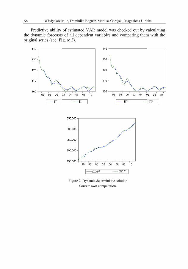
Predictive ability the dynamic forecastsoriginal series (see: Fi
Milo, Dominika Bogusz, Mariusz Górajski, Magdalena Ulric
of estimated VAR model was checked out by cs of all dependent variables and comparing themigure 2).
Figure 2. Dynamic deterministic solution
Source: own computation.
chs
calculating m with the
Notes on Some Optimal Monetary Policy Rules: the Case of Poland 69
Table 4. Ex post errors for dynamic deterministic forecast
Ex post error GDP π πe
MAE 1815,82 0,96 0,81 MAPE (%) 0,74 0,91 0,76 RMSE 2196,41 1,24 1,03
Source: own computation. Mean ex post absolute prediction errors for our VAR model (4) are low (see
MAPE in Table 4) – all errors do not exceed 1%. Thus, the model has very good ex post prognostic features and it is reasonable to use it in optimal control model solving.
5. Analysis of optimal solutions In this section we analyse the optimal solution of proposed version of
optimal control of monetary policy model for the two cases: in the first case it is assumed that decision makers focus only on inflation rate (Scenario 1), and in the second case output gap is also included into the goal functional (Scenario 2).
In the sequel, we use the Euclidian distance (average standard deviation measure) between optimal and empirical values of and its trend or target values given by:
1.
5.1. Scenario 1 It is assumed that the goal of the monetary policy is to achieve the inflation
rate target. Thus, we minimize only the expected distance of inflation rate from its target level. Therefore the cost functional takes the form:
0.9991
0.0011
.
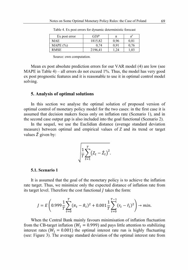
When the Central Bank mainly favours minimisation of inflation fluctuation
from the CB-target inflation 0.999 and pays little attention to stabilizing interest rates 0.001 the optimal interest rate run is highly fluctuating (see: Figure 3). The average standard deviation of the optimal interest rate from
Władysław Milo, Dominika Bogusz, Mariusz Górajski, Magdalena Ulrichs 70
its trend is equal to 2.61 . . while the average standard deviation of the empirical interest rate from its trend is smaller and equals to 2.1 . . It is worth mentioning that the largest fluctuations are at the beginning of the considered period. However, during the second half of the analysed period one may observe that the optimal path is closer to the trend in comparison to the empirical interest rate.
Figure 3. Scenario 1 – values of interest rates, where R* is the optimal path,
R is the empirical path and Rhp is the empirical trend path Source: own computation.
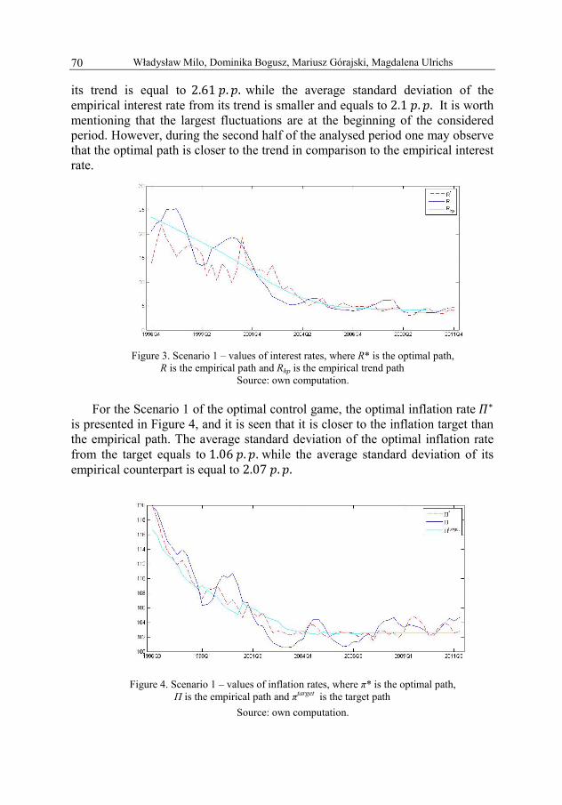
For the Scenario 1 of the optimal control game, the optimal inflation rate
is presented in Figure 4, and it is seen that it is closer to the inflation target than the empirical path. The average standard deviation of the optimal inflation rate from the target equals to 1.06 . . while the average standard deviation of its empirical counterpart is equal to 2.07 . .
Figure 4. Scenario 1 – values of inflation rates, where π* is the optimal path,
П is the empirical path and πtarget is the target path
Source: own computation.

Notes on Some Optimal Monetary Policy Rules: the Case of Poland 71
Despite that the strong fluctuations of optimal interest rate cause relatively large fluctuations of optimal (see Figure 5) the optimal GDP is less fluctuating than empirical (average standard deviation of the optimal growth rates from their trend values is equal to 1.67 . . while the average standard deviation of the empirical growth rates from their trend values equals even 1.83 . .). Under our version of the model the CB optimal rule of choice brings less GDP-growth fluctuations than the actual monetary policy used by the CB reflected in empirical series of GDP.
Figure 5. Scenario 1 – values of real GDP growth rates (corresponding period of previous year = 100), where gGDP* is the optimal path, gGDP is the empirical path and gGDPHP
is the dynamic of trend of the empirical GDP
Source: own computation. Summing up obtained results, it may be said that during the last 15 years it
was possible to get inflation rate closer to the target inflation, by the incitements of larger fluctuations of interest rates, especially during the first 5 years. High fluctuations of interest rates are unacceptable for the financial stability reasons. However, surprisingly instability of optimal interest rates influences but does not destabilize the optimal GDP growth rates.
5.2. Scenario 2 Under this scenario, we minimize the weighted sum of quadratic distances of
inflation from its target level, the empirical GDP and interest rates from their long-term trends. We assume that inflation and output variability are equally weighted (similar scenario was considered in: Batini and Haldane 1999). Thus, we consider model of monetary policy with the cost functional of the form:
1998Q3 2001Q1 2003Q3 2006Q1 2008Q3 2011Q1-2
0
2
4
6
8
10
12
14
gGDP*
gGDPgGDP
HP

Władysław Milo, Dominika Bogusz, Mariusz Górajski, Magdalena Ulrichs 72
0.9991
0.5 0.5
0.0011
.
Figure 6. Values of interest rates, where R* is the optimal path, R is the empirical path
and Rhp is the empirical trend path Source: own computation.
The average standard deviation of the optimal interest rate from its trend is equal to 1.79 . . (see: Figure 6). This means that the optimal control rates have smaller fluctuations than the empirical path rates and smaller in comparison to the optimal control path values for the first scenario.
Figure 7. Scenario 2 – values of inflation rates, where π* is the optimal path, П is the empirical path and πtarget is the target path
Source: own computation.
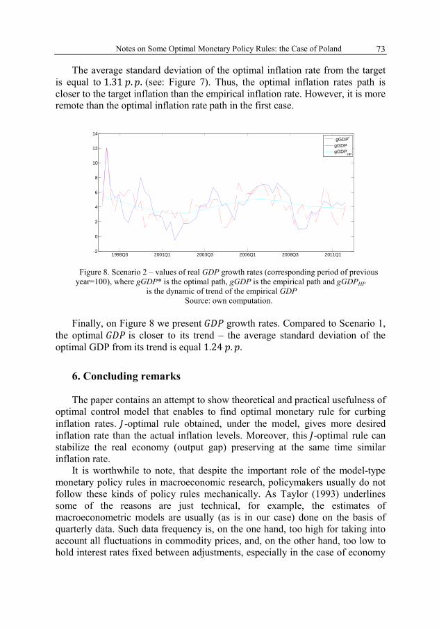
Notes on Some Optimal Monetary Policy Rules: the Case of Poland 73
The average standard deviation of the optimal inflation rate from the target is equal to 1.31 . . (see: Figure 7). Thus, the optimal inflation rates path is closer to the target inflation than the empirical inflation rate. However, it is more remote than the optimal inflation rate path in the first case.
Figure 8. Scenario 2 – values of real GDP growth rates (corresponding period of previous
year=100), where gGDP* is the optimal path, gGDP is the empirical path and gGDPHP is the dynamic of trend of the empirical GDP
Source: own computation. Finally, on Figure 8 we present growth rates. Compared to Scenario 1,
the optimal is closer to its trend – the average standard deviation of the optimal GDP from its trend is equal 1.24 . .
6. Concluding remarks The paper contains an attempt to show theoretical and practical usefulness of
optimal control model that enables to find optimal monetary rule for curbing inflation rates. -optimal rule obtained, under the model, gives more desired inflation rate than the actual inflation levels. Moreover, this -optimal rule can stabilize the real economy (output gap) preserving at the same time similar inflation rate.
It is worthwhile to note, that despite the important role of the model-type monetary policy rules in macroeconomic research, policymakers usually do not follow these kinds of policy rules mechanically. As Taylor (1993) underlines some of the reasons are just technical, for example, the estimates of macroeconometric models are usually (as is in our case) done on the basis of quarterly data. Such data frequency is, on the one hand, too high for taking into account all fluctuations in commodity prices, and, on the other hand, too low to hold interest rates fixed between adjustments, especially in the case of economy
1998Q3 2001Q1 2003Q3 2006Q1 2008Q3 2011Q1-2
0
2
4
6
8
10
12
14
gGDP*
gGDPgGDP
HP
Władysław Milo, Dominika Bogusz, Mariusz Górajski, Magdalena Ulrichs 74
falling into recession. Usually any model or method modifications that help to solve practical economic problems result in more complex rules. It does not yet mean that in empirical research the policy rules should be treated as discretion policy rules.
References Ball L. (1997), Efficient Rules for Monetary Policy, NBER Working Paper No. 5952. Baranowski P. (2008), Reguła Taylora oraz jej rozszerzenia – przegląd badań, Gospodarka
Narodowa, 7–8, 1–23. Baranowski P. (2011), Reguła polityki pieniężnej dla Polski – porównanie wyników różnych
specyfikacji, Oeconomia Copernicana No. 3, 5–21. Batini N., Haldane A. (1999), Forward-Looking Rules for Monetary Policy, NBER Working Paper 7416. Brzoza-Brzezina M. (2011), Polska polityka pieniężna. Badania teoretyczne i empiryczne,
Wydawnictwo C.H. Beck, Warszawa. Clarida R., Gali J., Gertler M. (1998), Monetary policy rules in practice. Some international
evidence, European Economic Review, 42, 1033–1067. Clarida R., Gali J., Gertler M. (1999), The Science of Monetary Policy: a New Keynesian
Perspective, CEPR Discussion Paper No. 2139. Demchuk O., Łyziak T., Przystupa J., Sznajderska A., Wróbel E. (2012), Monetary policy
transmission mechanism in Poland. What do we know in 2011?, National Bank of Poland Working Paper No. 116.
Gali J. (2007), Monetary Policy, Inflation, and the Business Cycle, CREI and UPF. Hodrick R.J., Prescott E.C. (1997), Postwar U.S. Business Cycles: An Empirical Investigation,
Journal of Money, Credit, and Banking, 29, 1, 1–16. Judd J.P., Rudebusch G.D. (1998), Taylor’s Rule and the Fed: 1970-1997, FRBSF Economic
Review No. 3. Kłos B., Kokoszczyński R., Łyziak T., Przystupa J., Wróbel E. (2004), Modele strukturalne
w prognozowaniu inflacji w Narodowym Banku Polskim, National Bank of Poland Working Paper No. 180.
Lenart Ł., Pipień M. (2012), Almost periodically correlated time series in business fluctuations analysis, National Bank of Poland Working Paper No. 107.
Łyziak T. (2002), Monetary transmission mechanism in Poland. The strength and delays, National Bank of Poland Working Paper No. 26.
Łyziak T., Przystupa J., Sznajderska A., Wróbel E. (2012), Money in monetary policy, National Bank of Poland Working Paper No. 135.
MacKinnon J.G. (1996), Numerical distribution functions for unit root and cointegration tests, Journal of applied econometrics, 11, 6, 601–618.
Maravall A., del Rio A. (2001), Time aggregation and the Hodrick-Prescott filter. Banco de Espa˜na Servicio de Estudios Documento de Trabajo No. 0108.
McCallum B.T. (1998), Issues in the Design of Monetary Policy Rules, NBER Working Paper 6016. McCallum B.T., Nelson E. (2000), Timeless Perspective vs. Discretionary Monetary Policy in
Forward-looking Models, NBER Working Paper No. 7915. Mehra Y.P. (1999), A Forward-Looking Monetary Policy Reaction Function, Federal Reserve
Bank of Richmond Economic Quarterly, 85, 2, 33–53. Mishkin F. S. (1996), The channels of monetary transmission: lessons for monetary policy, NBER
Working Paper Series No. 5464. Orphanides A., Wilcox D. (2002), The Opportunistic Approach to Disinflation, International
Finance, 5, 1, 47–71.
Notes on Some Optimal Monetary Policy Rules: the Case of Poland 75
Polito V., Wickens M. (2012), Optimal monetary policy using an unrestricted VAR, Journal of Applied Econometrics, 27, 525–553.
Postek Ł. (2011), Nieliniowy model mechanizmy transmisji monetarnej w Polsce w latach 1999-2009. Podejście empiryczne, National Bank of Poland Working Paper No. 253.
Rotemberg J., Woodford M. (1998), Interest-Rate Rules in an Estimated Sticky Price Model, NBER Working Paper No. 6618.
Rudebusch G., and Svensson, L.E.O. (1999), Policy Rules for Inflation Targeting, NBER Working Paper No. 6512.
Sack B. (2000), Does the Fed act gradually? A VAR analysis, Journal of Monetary Economics, 46,1, 229–256.
Sławiński A. (2011), Polityka pieniężna, Wydawnictwo C.H. Beck, Warszawa. Solow R., Taylor J.B. (1998), Inflation, unemployment, and Monetary Policy, The MIT-Press. Svensson L. (1997), Inflation Forecast Targeting: Implementing and Monitoring Inflation Targets,
European Economic Review, 41, 6, 1111–1146. Svensson L. (2000), Open-economy inflation targeting, Journal of International Economics, 50, 1,
155–183. Taylor J.B. (1993), Discretion versus policy rules in practice, Carnegie-Rochester Conference
Series on Public Policy, 39, 195–214. Taylor J.B. (1999), Monetary Policy Rules, NBER Book Series Studies in Business Cycles No. 31,
University of Chicago Press. Urbańska M. (2002), Polityka monetarna: współczesna teoria i analiza empiryczna dla Polski,
National Bank of Poland Working Paper No. 148. Woodford M. (1999), Optimal Monetary Policy Inertia, Institute for International Economic
studies Stockholm University, Seminar Paper No. 666. Woodford M. (2001), The Taylor Rule and Optimal Monetary Policy, The American Economic
Review, 91, 2, 232–237. Woodford M. (2003), Interest and Prices, PUP, Princeton. Wróbel E., Pawłowska M. (2002), Monetary transmission in Poland: some evidence on interest
rate and credit channels, National Bank of Poland Working Paper No. 24. Zabczyk J. (1996), Chance and decision: stochastic control in discrete time, Scuola Normale
Superiore.
Władysław Milo, Dominika Bogusz, Mariusz Górajski, Magdalena Ulrichs
O OPTYMALNYCH REGUŁACH POLITYKI PIENIĘŻNEJ: PRZYPADEK POLSKI
Streszczenie W artykule przestawiono wstępne wyniki badania dotyczącego zastosowania modelu
optymalnego sterowania opisującego reguły polityki pieniężnej. Rozwiązanie takiego modelu umożliwiło znalezienie użytecznych form optymalnych reguł polityki pieniężnej w przypadku przyjętych dwóch scenariuszy. Reguły te zostały wyprowadzone w oparciu o liniowy model VAR(s) opisujący zmiany odchylenia logarytmów stóp wzrostu PKB od ich długookresowego trendu, odchylenia empirycznych poziomów CPI od celu inflacyjnego NBP, odchylenia oczekiwań inflacyjnych od ich długookresowego trendu, jak również w oparciu o dwie postaci funkcjonału J-pozwalające na wyznaczenie różnych trajektorii optymalnych poziomów stóp procentowych NBP. Teoretyczne wartości tych stóp, ustalone w oparciu o polskie dane kwartalne, stanowiły podstawę do określenia odpowiadających im poziomów inflacji, stóp wzrostu PKB jak również do porównania ich z rzeczywistymi stopami procentowymi NBP.
Władysław Milo, Dominika Bogusz, Mariusz Górajski, Magdalena Ulrichs 76
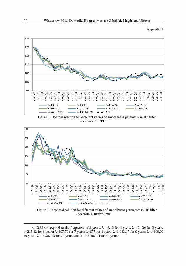
Appendix 1
Figure 9. Optimal solution for different values of smoothness parameter in HP filter
- scenario 1, CPI3
Figure 10. Optimal solution for different values of smoothness parameter in HP filter - scenario 1, interest rate
.
3λ=13,93 correspond to the frequency of 3 years; λ=43,15 for 4 years; λ=104,36 for 5 years;
λ=215,32 for 6 years; λ=397,70 for 7 years; λ=677 for 8 years; λ=1 083,17 for 9 years; λ=1 600,00 10 years; λ=26 307,95 for 20 years; and λ=133 107,94 for 30 years.

Notes on Some Optimal Monetary Policy Rules: the Case of Poland 77
Figure 11. Optimal solution for different values of smoothness parameter in HP filter
- scenario 2, CPI
Figure 12. Optimal solution for different values of smoothness parameter in HP filter - scenario 2, interest rate.