Optimal Monetary Policy Rules, Asset Prices and

Credit Frictions ∗

Ester Faia†

Universitat Pompeu FabraTommaso Monacelli‡

IGIER, Universita Bocconi and CEPR

January 2005

Abstract

We study optimal monetary policy in two prototype economies with sticky prices and creditmarket frictions. In the first economy, credit frictions apply to the financing of the capital stock,generate acceleration in response to shocks and the ”financial markup” (i.e., the premium onexternal funds) is countercyclical and negatively correlated with the asset price. In the secondeconomy, credit frictions apply to the flow of investment, generate persistence, and the financialmarkup is procyclical and positively correlated with the asset price. We model monetary policyin terms of welfare-maximizing interest rate rules. The main finding of our analysis is that strictinflation stabilization is a robust optimal monetary policy prescription. The intuition is that, inboth models, credit frictions work in the direction of dampening the cyclical behavior of inflationrelative to its credit-frictionless level. Thus neither economy, despite yielding different inflationand investment dynamics, generates a trade-off between price and financial markup stabilization.A corollary of this result is that reacting to asset prices does not bear any independent welfarerole in the conduct of monetary policy.

Keywords: Optimal monetary policy rules, financial distortions, price stability, asset prices.

∗First draft May 2004. We thank Pierpaolo Benigno, Fiorella de Fiore, Harris Dellas, Jordi Galı, StephanieSchmitt-Grohe, Michael Woodford and participants to the 2004 ESSIM-CEPR conference for useful comments. Allerrors are our own responsibility.

†Correspondence to Universitat Pompeu Fabra, Ramon Trias Fargas 25, Barcelona, Spain. E-mail: es-ter.faia@econ.upf.es, homepage: http://www.econ.upf.es/˜faia/.

‡Correspondence to IGIER Universita’ Bocconi, Via Salasco 3/5, 20136 Milan, Italy. Email:tommaso.monacelli@uni-bocconi.it, Tel: +39-02-58363330, Fax: +39-02-58363332, Web page: www.igier.uni-bocconi.it/monacelli.

1

1 Introduction

In this paper we study optimal monetary policy rules in an economy with nominal rigidities and

credit market imperfections. Our interest is twofold. First, we aim at driving the attention of

the recent literature on a typology of market distortions whose role has been largely neglected in

the normative analysis of monetary policy. This is surprising, considering the increasing emphasis

placed on financial factors in the studying of business cycles (starting with Bernanke and Gertler

(1989)). Second, we aim at assessing - from a welfare-based perspective - the role that asset prices

and or other financial indicators should play in the optimal setting of monetary policy rules.

The latter issue has been recently the object of an intense debate, within both policy and

academic circles, in light of the asset price inflation phenomenon of the late nineties, followed

by the burst of the alleged financial bubble at the beginning of the new century.1 However, the

theoretical literature linking asset prices, monetary policy and financial frictions in dynamic general

equilibrium models has been scant. Bernanke and Gertler (2001) (BG henceforth) compare the

performance of alternative interest rate rules, including some that feature a reaction to asset price

movements. Their main conclusion is that there is negligible stabilization gain from including asset

prices as independent arguments in the rules. Gilchrist and Leahy (2002) employ a similar (financial

accelerator) framework, and evaluate the ability of alternative rules to have their reference model

mimic as close as possible the dynamics of a real business cycle model. Cecchetti et al. (2002)

contend with BG, and argue that the desirability of including asset prices as separate arguments

in interest rate rules is likely to depend on the underlying source of shocks.2

The common shortcoming of this literature is that it completely abstracts from strict welfare

considerations. The metric adopted for the evaluation of the relative performance of policy rules

is typically an output-inflation volatility frontier. This makes it hard to correctly rank alternative

specifications for monetary policy, and to safely draw normative conclusions about the desirability

for monetary policy to react to asset price movements. It is this consideration that essentially

motivates the present paper.

A common argument of the contenders of the BG view is that asset price movements may be

driven by non-fundamental shocks to the financial side of the economy - i.e., bubbles - and that a

monetary authority which aims at reaching a first-best allocation should convey those movements

back to their efficient evolution.3 However, it seems hard to justify a systematic response of

the monetary authority to asset price movements only on the possibility of occurrence of bubble

1See Gilchrist and Leahy (2002) for a survey.2Iacoviello (2004) analyzes monetary policy in a model with credit cycles a la Kyotaki and Moore (1997) and

housing, and concludes that reacting to asset prices does not improve macroeconomic stability.3See also Dupor (2003).

1

dynamics (Bernanke 2002). For this reason we re-focus the analysis in a more genuine public finance

spirit and solely in the presence of fundamental shocks (e.g., to productivity and/or government

expenditures).

Our baseline economy will feature three types of distortions. First, monopolistic competition

in goods markets, which forces average output below the socially optimal level. Second, adjustment

costs in nominal goods prices, which entail a direct resource cost, as well as a misalignment between

the marginal utility of consumption and leisure due to time variations in price markups. Third,

informational frictions, in the form of endogenous agency costs, which characterize the relationship

between borrowers and lenders in the credit market. In this context, and in deviation from the

Modigliani-Miller theorem, the evolution of firms’ net worth affects both the cost of access to credit

and the price of capital. Yet, in turn, these developments feedback onto firms’ financial position,

further affecting investment and capital accumulation. Agency costs, per se, have a twofold effect.

In the long run, they produce an inefficiently low level of capital, and hence output, since the

economy suffers a deadweight loss associated to the monitoring activity of the lender. In the short-

run, the presence of a time-varying ”financial markup” distorts the dynamic allocation of capital

and investment.

The recent optimal monetary policy literature has dealt with the role of distortions in alterna-

tive ways. The vast majority of papers specify a complementary (and arguably unrealistic) role of

fiscal policy to neutralize the steady-state distortions related to market power in goods and/or labor

markets. This assures that, if the only left distortion is price stickiness, the average level of output

coincides (under zero inflation) also with the efficient one, allowing to neglect the role of stochastic

uncertainty on the mean level of those variables which are relevant for welfare.4 The approach

followed here, as in Kollmann (2003a, 2003b) and Schmitt-Grohe and Uribe (2003, 2004b), and

unlike much of the so-called New Keynesian literature, allows to study optimal policy in a dynamic

economy that evolves around a steady-state which remains distorted. Importantly, in our context,

the steady state of the economy will be distorted not only by the presence of nominal rigidities and

market power in goods markets, but also by the presence of monitoring costs in credit markets. As

emphasized by Kim et al. (2003) and Schmitt-Grohe and Uribe (2004b), this strategy requires that

an accurate evaluation of welfare be based on a higher order approximation of all the conditions

that characterize the competitive equilibrium of the economy.5

4To name a few, Rotemberg and Woodford (1997), Clarida, Gali and Gertler (1999), King and Wolman (1999),Erceg, Henderson and Levin (2000), culminating with Woodford (2003).

5Alternatively, Benigno and Woodford (2004) show how to preserve the linear-quadratic form of an optimal policyproblem in the case in which the economy fluctuates around a non-efficient steady-state. This per se requires takinga second order approximation of (some of) the underlying equilibrium conditions.

2

1.1 Credit Frictions and Financial Markups: Two Theoretical Frameworks

We will articulate our analysis of optimal monetary policy on two general equilibrium models in

which credit market frictions and asset price movements play a role. The first model is based

on Bernanke, Gertler and Gilchrist (1999), while the second model is a sticky-price monetary

extension of Carlstrom and Fuerst (1997). The common denominator to the two models is that

credit frictions take the form of endogenous agency costs in the relationship between lenders and

borrowers (typically entrepreneurs). These costs emerge when verifying the return of borrowers’

(risky) projects is costly for the lender, a feature that generates a typical moral hazard problem.6

There are however important differences. In the first framework, labelled below as capital-

acceleration model (KA model henceforth), credit frictions apply to the financing of the stock of

capital owned by entrepreneurs. In equilibrium, firms face a spread between the cost of internal

and external funds (the external finance premium). The key element of this model lies in the coun-

tercyclical behavior of the finance premium, a mechanism that generates an effect of acceleration

in response to shocks. Movements in asset prices act to reinforce this mechanism, by affecting the

value of the capital stock and hence entrepreneurs’ balance sheets. This asset price effect is akin to

the credit-cycle phenomenon stressed by Kyotaki and Moore (1997). The main regularity we are

interested in singling out in this model is that, as a result, asset prices and finance premium are

negatively correlated.

The second model we analyze is labelled investment-propagation model (IP henceforth). In

this framework, credit frictions apply to the financing of the investment flow. Two are the main

differences with respect to the KA model. First, rather than acceleration, the IP model generates

equilibrium propagation of shocks (i.e., hump-shaped dynamics of output and investment). This

difference stems crucially from the equilibrium sluggish behavior of entrepreneurs’ net worth. This

feature is such that, e.g., a rise in productivity, brings about an initial rise in borrowing needs

and therefore in the marginal cost of investment. However, as net worth accumulates over time,

it generates a corresponding shift in the investment supply curve, thereby subsequently lowering

the marginal cost of investment. This effect generates a second crucial difference in the IP model,

namely that the external finance premium behaves procyclically, and is directly proportional to

the behavior of the relative price of investment goods (asset price). Thus, asset price and finance

premium are positively correlated in this framework.

An important consequence is that the interpretation of asset price movements differs in the

two models. In the KA model, fluctuations in asset prices are introduced somewhat exogenously.

More precisely, they would disappear in the absence of adjustment costs on capital (a scenario that

6In turn, all these models are extensions of the seminal contribution of Bernanke and Gertler (1989) who incor-porate in general equilibrium the costly state verification framework of Gale and Hellwig (1985).

3

would not correspond to the absence of credit frictions)7. Rather, in the IP model, movements in

the Tobin’s q are genuinely endogenous, in the sense that they relate fundamentally to the presence

of investment financing frictions.

Therefore, and more importantly for our purposes, the public finance interpretation of asset

price movements differs in the two models. In the IP model, unlike the KA model, asset price

fluctuations are akin to financial markups cyclical variations. In fact, investment goods must sell

at a markup over consumption goods to compensate the lender for the costs of imperfect monitoring.

In this respect, their behavior resembles the one of a tax affecting the intertemporal allocation of

investment. The corresponding financial markup concept in the KA model is the external finance

premium on the amount borrowed in excess of internal funds. In equilibrium, capital accumulation

must be such that the marginal cost of external funds is equated to the rate of return on capital.

Hence, in this case, a markup is applied to a relative return as opposed to a relative price.

The main finding of our analysis is that strict inflation stabilization is a robust optimal mon-

etary policy prescription. Noticeably, this holds regardless of the two models delivering opposite

predictions on the cyclical behavior of the financial markup. The basic intuition works as follows.

Although the dynamics of inflation and investment differ sharply across models, we find that in

both cases credit frictions work in the direction of dampening the cyclical behavior of inflation

relative to a hypothetical environment in which the same frictions are absent. Hence, when credit

frictions generate acceleration and over-investment (as in the KA model) we find that inflation

falls below its steady state but, at the margin, it rises relative to its level in the absence of credit

frictions. On the other hand, when credit frictions generate persistence and, in the short run,

keep investment below its credit-frictionless level (as in the IP model), also inflation remains below

its credit-frictionless benchmark. In both cases, a manipulation of the real interest rate does not

generate any inherent trade-off between stabilizing the price markup and stabilizing the financial

markup. A corollary of this result is that reacting to asset prices does not bear any independent

welfare role in the conduct of monetary policy.

The remainder of the paper is organized as follows. Section 2 and 6 introduces the main

differences in the theoretical frameworks analyzed in the paper. Section 3 describes our calibration

and solution strategy. Section 4 presents results on the equilibrium dynamics.. Section 5 illustrates

our welfare metric and section 7 concludes.

7This does not deny of course that movements in asset prices are magnified in the KA model due to an endogenousinteraction with firms’ balance sheets.

4

2 Capital-Acceleration (KA) Model

The first model we analyze builds on Bernanke, Gertler and Gilchrist (1999) financial accelerator

model. We will present this framework in more detail, while later on emphasizing only the basic

differences in the IP model.8

2.1 Households (Lenders)

There is a continuum of households, each indexed by i ∈ (0, 1). They consume a composite finalgood, invest in safe bank deposits, supply labor, and own shares of a monopolistic competitive

sector that produces differentiated varieties of goods. The representative household chooses the

set of processes Ct, Nt∞t=0 and one-period nominal deposits Dt∞t=0, taking as given the set ofprocesses Pt, Wt, (1 +Rn

t )∞t=0 and the initial condition D0 to maximize:

W0 ≡ E0

( ∞Xt=0

βtU(Ct,Nt)

)(1)

subject to the sequence of budget constraints:

PtCt +Dt+1 ≤ (1 +Rnt )Dt +WtNt +Υt + Tt (2)

where Ct is workers’ consumption of the final good,Wt is the nominal wage, Nt is total labor hours,

Rnt is the nominal net interest rate paid on deposits, Υt are the nominal profits that households

receive from running production in the monopolistic sector and Tt are lump sum taxes/transfers

from the fiscal authority. The first order conditions of the above problem read as follows:

Uc,t = β(1 +Rnt )Et

½Uc,t+1

PtPt+1

¾(3)

Uc,tWt

Pt= −Un,t (4)

limj→∞

(1 +Rnt+j)

−1Dt+j = 0 (5)

with the addition of (2) holding with equality.

8An alternative to the KA framework, still featuring effects of financial acceleration (or ”credit cycles”), wouldhave been the model of Kyotaki and Moore (1997). See below for a discussion of why the latter model would havebeen incongrous for the analysis of optimal policy conducted here.

5

2.2 Unfinished-Capital Producers

A competitive sector of capital producers combine investment (expressed in the same composite as

the final good, hence with price Pt) and existing (depreciated) capital stock to produce unfinished

capital goods. This activity entails physical adjustment costs. The corresponding CRS production

function is φ( ItKt) Kt, so that capital accumulation obeys:

Kt+1 = (1− δ)Kt + φ(ItKt) Kt (6)

where φ(•) is increasing and convex.Define Qt as the re-sell price of the capital good. Capital producers maximize profits Qt φ(

ItKt)

Kt − PtIt, implying the following first order condition:

Qt φ0(ItKt) = Pt (7)

2.3 Entrepreneurs (Borrowers)

The activity of the second set of agents, the entrepreneurs, is at the heart of the model. These

agents are risk neutral. They purchase unfinished capital from the capital producers at the price

Qt and transform it into finished capital to be rented to intermediated goods producers. To finance

the purchase of unfinished capital they employ internal funds but need also to acquire an external

loan from a financial intermediary. The relationship with the lender is subject to an agency cost

problem, which forces the entrepreneur to pay a premium on the loan. We will elaborate below on

this point.

We assume that the entrepreneurs are finitely lived (with θ being the probability of dying in

each period ) and risk neutral. This assumption assures that entrepreneurial consumption occurs

to such an extent that self-financing never occurs and borrowing constraints on loans are always

binding. Resorting to the law of large numbers and to the characteristics of the loan contract will

allow a convenient aggregation for these agents’ decisions. As consumers, the entrepreneurs act as

simple finitely lived agents who in every period consume a constant share of their wealth.

Let’s define by Zt the nominal rental rate of capital. The nominal income from holding

one unit of finished capital is composed of the rental rate plus the re-sell price of capital (net of

depreciation and physical adjustment costs):

Ykt ≡ Zt +Qt

µ(1− δ)− φ

0(ItKt)ItKt+ φ(

ItKt)

¶Hence the return to entrepreneurs from holding a unit of capital between t and t+ 1 amounts to:

6

(1 +Rkt+1) ≡

Ykt+1

Qt(8)

2.4 The Loan Contract Between the Borrower and the Financial Intermediary

At the end of period t a continuum of entrepreneurs (indexed by j) need to finance the purchase

of new capital Kjt+1 that will be used for production in period t + 1. In order to acquire a loan

the entrepreneurs have to engage in a financial contract before the realization of an idiosyncratic

shock ω(j) (with a payoff paid after the realization of the same shock). The idiosyncratic shock

has positive support, is independently distributed (across entrepreneurs and time) with a uniform

distribution, F (ω), with unitary mean, and density function f(ω). The return of the entrepreneurial

investment is observable to the outsider only through the payment of a monitoring cost µYkt+1K

jt+1,

where µ is the fraction of lender’s output lost in monitoring costs. Hence this cost is proportional

to the expected return on capital purchased at the end of period t .

Before entering the loan contract agreement each entrepreneur owns end-of-period internal

funds for a nominal amount NW jt+1 and seeks to finance the purchase of new capital QtK

jt+1. We

assume that the required funds for investment exceed internal funds. Hence in every period each

entrepreneur seeks for a loan (in nominal terms):

Ljt+1 = QtK

jt+1 −NW j

t+1 ≥ 0 (9)

The financial contract assumes the form of an optimal debt contract a la Gale and Hellwig

(1985). When the idiosyncratic shock to capital investment is above the cut-off value which deter-

mines the default states the entrepreneurs repay a fixed amount (1 + RLt+1). On the contrary, in

the default states, the bank monitors the investment activity and repossesses the assets of the firm.

Default occurs when the return from the investment activity Ykt+1K

jt+1 falls short of the amount

that needs to be repaid (1+RLt+1)L

jt+1. Hence the default space is implicitly defined as that range

for ω such that :

ωjt+1 <jt+1 ≡

(1 +RLt+1)L

jt+1

Ykt+1K

jt+1

(10)

where jt+1 is a cut-off value for the idiosyncratic productivity shock, which is determined endoge-

nously in the general equilibrium9.

The timing of events can be summarized as follows

• End of period t.

9The fact that default is an equilibrium phenomenon is a crucial difference between the endogenous agency costmodels (as the ones employed here) and the credit-cycle models a la Kyotaki and Moore (1997).

7

1. Entrepreneur j holds nominal net worth NW jt+1, acquires loan Lj

t+1 to purchase new capital

Kjt+1 which will be available to rental market and production in period t+ 1.

2. Idiosyncratic shock ωjt+1 to the newly purchased capital realizes.

• Period t+ 1.

1. Aggregate shocks to productivity and government consumption realize.

2. Entrepreneur supplies capital services to rental market.

3. Entrepreneur pays off loan services to the lender.

4. Current net worth realizes.

2.5 Optimal Contract

Let’s define by Γ( j) and 1−Γ( j) the fractions of net capital output received by the lender and

the entrepreneur respectively. Hence we have:

Γ( jt+1) ≡

Z jt+1

0ωjt+1f(ω)dω +

jt+1

Z ∞

t+1

f(ω)dω

Expected monitoring costs are defined as:

µM( jt+1) ≡

Z jt+1

0ωjt+1f(ω)dω

Hence the net share accruing to the lender is Γ( jt+1)−µM( j

t+1). The return paid on deposits is

given by the safe rate (1 +Rnt ), which as such corresponds, for the lender, to the opportunity cost

of financing capital.

The participation constraint for the lender states that the expected return from the lending

activity should not fall short of the opportunity cost of finance:

Ykt+1K

jt+1(Γ(

jt+1)− µM( j

t+1)) ≥ (1 +Rnt )(QtK

jt+1 −NW j

t+1) (11)

The contract specifies a pairn

jt+1, L

jt+1

owhich solves the following maximization problem:

Max (1− Γ( jt+1))Yk

t+1Kjt+1 (12)

subject to the participation constraint (11). Let χt be the lagrange multiplier on (11). First order

conditions with respect to jt+1 and Kj

t+1 read:

8

Γ0( jt+1) = χt(Γ

0( jt+1)− µM 0( j

t+1)) (13)

(1 +Rkt+1)

(1 +Rnt )

³(1− Γ( j

t+1)) + χt(Γ(jt+1)− µM( j

t+1))´= χt (14)

In addition, with χt > 0, (11) must hold with equality.

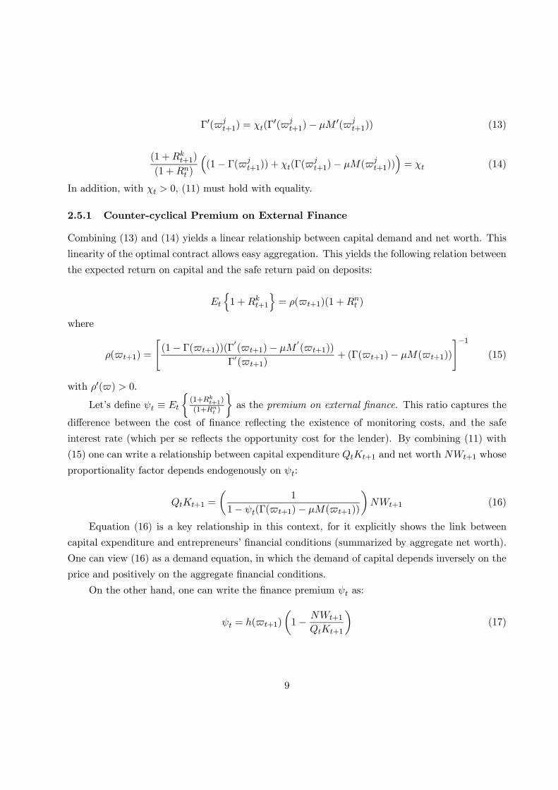
2.5.1 Counter-cyclical Premium on External Finance

Combining (13) and (14) yields a linear relationship between capital demand and net worth. This

linearity of the optimal contract allows easy aggregation. This yields the following relation between

the expected return on capital and the safe return paid on deposits:

Et

n1 +Rk

t+1

o= ρ( t+1)(1 +Rn

t )

where

ρ( t+1) =

"(1− Γ( t+1))(Γ

0( t+1)− µM

0( t+1))

Γ0( t+1)+ (Γ( t+1)− µM( t+1))

#−1(15)

with ρ0( ) > 0.

Let’s define ψt ≡ Et

½(1+Rk

t+1)

(1+Rnt )

¾as the premium on external finance. This ratio captures the

difference between the cost of finance reflecting the existence of monitoring costs, and the safe

interest rate (which per se reflects the opportunity cost for the lender). By combining (11) with

(15) one can write a relationship between capital expenditure QtKt+1 and net worth NWt+1 whose

proportionality factor depends endogenously on ψt:

QtKt+1 =

µ1

1− ψt(Γ( t+1)− µM( t+1))

¶NWt+1 (16)

Equation (16) is a key relationship in this context, for it explicitly shows the link between

capital expenditure and entrepreneurs’ financial conditions (summarized by aggregate net worth).

One can view (16) as a demand equation, in which the demand of capital depends inversely on the

price and positively on the aggregate financial conditions.

On the other hand, one can write the finance premium ψt as:

ψt = h( t+1)

µ1− NWt+1

QtKt+1

¶(17)

9

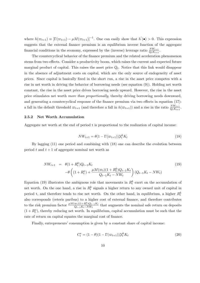
where h( t+1) ≡ [Γ( t+1)− µM( t+1)]−1. One can easily show that h0(•) > 0. This expression

suggests that the external finance premium is an equilibrium inverse function of the aggregate

financial conditions in the economy, expressed by the (inverse) leverage ratio NWt+1

QtKt+1.

The countercyclical behavior of the finance premium and the related acceleration phenomenon

stems from two effects. Consider a productivity boom, which raises the current and expected future

marginal product of capital. This raises the asset price Qt. Notice that this link would disappear

in the absence of adjustment costs on capital, which are the only source of endogeneity of asset

prices. Since capital is basically fixed in the short run, a rise in the asset price competes with a

rise in net worth in driving the behavior of borrowing needs (see equation (9)). Holding net worth

constant, the rise in the asset price drives borrowing needs upward. However, the rise in the asset

price stimulates net worth more than proportionally, thereby driving borrowing needs downward,

and generating a countercyclical response of the finance premium via two effects in equation (17):

a fall in the default threshold t+1 (and therefore a fall in h( t+1)) and a rise in the ratioNWt+1

QtKt+1.

2.5.2 Net Worth Accumulation

Aggregate net worth at the end of period t is proportional to the realization of capital income:

NWt+1 = θ(1− Γ( t+1))Ykt Kt (18)

By lagging (11) one period and combining with (18) one can describe the evolution between

period t and t+ 1 of aggregate nominal net worth as

NWt+1 = θ(1 +Rkt )Qt−1Kt (19)

−θµ(1 +Rn

t ) +µM( t)(1 +Rk

t )Qt−1Kt

Qt−1Kt −NWt

¶(Qt−1Kt −NWt)

Equation (19) illustrates the ambiguous role that movements in Rkt exert on the accumulation of

net worth. On the one hand, a rise in Rkt signals a higher return to any owned unit of capital in

period t, and therefore tends to rise net worth. On the other hand, in equilibrium, a higher Rkt

also corresponds (ceteris paribus) to a higher cost of external finance, and therefore contributes

to the risk premium factorµM( t)(1+Rk

t )Qt−1Kt

Qt−1Kt−NWtthat augments the nominal safe return on deposits

(1 +Rnt ), thereby reducing net worth. In equilibrium, capital accumulation must be such that the

rate of return on capital equates the marginal cost of finance.

Finally, entrepreneurs’ consumption is given by a constant share of capital income:

Cet = (1− θ)(1− Γ( t+1))Yk

t Kt (20)

10

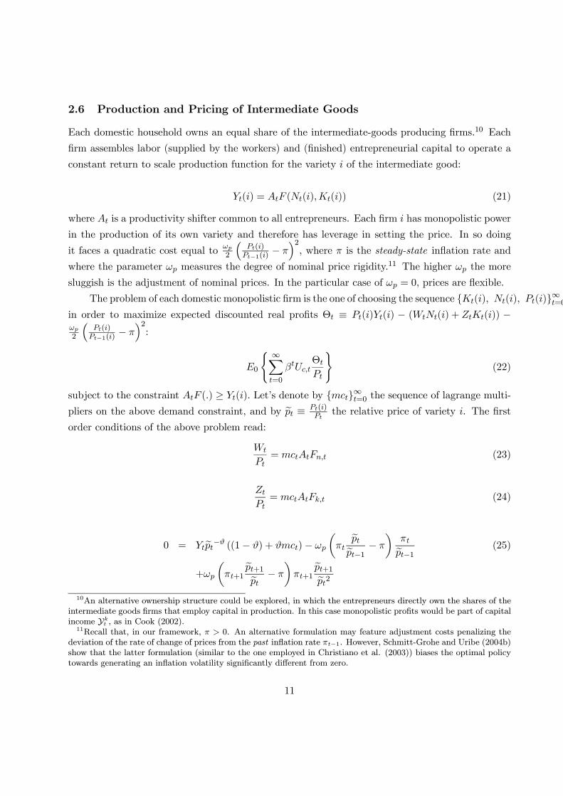
2.6 Production and Pricing of Intermediate Goods

Each domestic household owns an equal share of the intermediate-goods producing firms.10 Each

firm assembles labor (supplied by the workers) and (finished) entrepreneurial capital to operate a

constant return to scale production function for the variety i of the intermediate good:

Yt(i) = AtF (Nt(i),Kt(i)) (21)

where At is a productivity shifter common to all entrepreneurs. Each firm i has monopolistic power

in the production of its own variety and therefore has leverage in setting the price. In so doing

it faces a quadratic cost equal toωp2

³Pt(i)

Pt−1(i) − π´2, where π is the steady-state inflation rate and

where the parameter ωp measures the degree of nominal price rigidity.11 The higher ωp the more

sluggish is the adjustment of nominal prices. In the particular case of ωp = 0, prices are flexible.

The problem of each domestic monopolistic firm is the one of choosing the sequence Kt(i), Nt(i), Pt(i)∞t=0in order to maximize expected discounted real profits Θt ≡ Pt(i)Yt(i) − (WtNt(i) + ZtKt(i)) −ωp2

³Pt(i)

Pt−1(i) − π´2:

E0

( ∞Xt=0

βtUc,tΘt

Pt

)(22)

subject to the constraint AtF (.) ≥ Yt(i). Let’s denote by mct∞t=0 the sequence of lagrange multi-pliers on the above demand constraint, and by ept ≡ Pt(i)

Ptthe relative price of variety i. The first

order conditions of the above problem read:

Wt

Pt= mctAtFn,t (23)

Zt

Pt= mctAtFk,t (24)

0 = Ytept−ϑ ((1− ϑ) + ϑmct)− ωp

µπt

eptept−1 − π

¶πtept−1 (25)

+ωp

µπt+1

ept+1ept − π

¶πt+1

ept+1ept210An alternative ownership structure could be explored, in which the entrepreneurs directly own the shares of the

intermediate goods firms that employ capital in production. In this case monopolistic profits would be part of capitalincome Ykt , as in Cook (2002).11Recall that, in our framework, π > 0. An alternative formulation may feature adjustment costs penalizing the

deviation of the rate of change of prices from the past inflation rate πt−1. However, Schmitt-Grohe and Uribe (2004b)show that the latter formulation (similar to the one employed in Christiano et al. (2003)) biases the optimal policytowards generating an inflation volatility significantly different from zero.

11

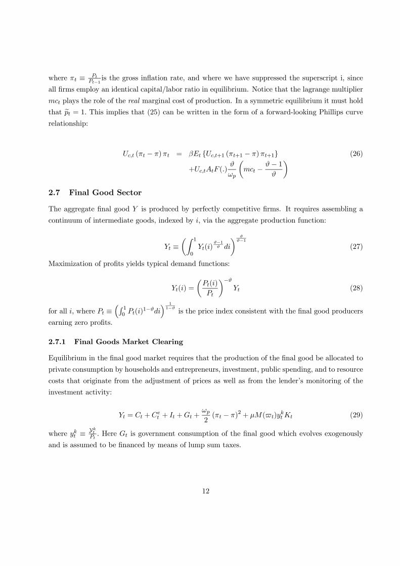
where πt ≡ PtPt−1 is the gross inflation rate, and where we have suppressed the superscript i, since

all firms employ an identical capital/labor ratio in equilibrium. Notice that the lagrange multiplier

mct plays the role of the real marginal cost of production. In a symmetric equilibrium it must hold

that ept = 1. This implies that (25) can be written in the form of a forward-looking Phillips curve

relationship:

Uc,t (πt − π)πt = βEt Uc,t+1 (πt+1 − π)πt+1 (26)

+Uc,tAtF (.)ϑ

ωp

µmct − ϑ− 1

ϑ

¶2.7 Final Good Sector

The aggregate final good Y is produced by perfectly competitive firms. It requires assembling a

continuum of intermediate goods, indexed by i, via the aggregate production function:

Yt ≡µZ 1

0Yt(i)

ϑ−1ϑ di

¶ ϑϑ−1

(27)

Maximization of profits yields typical demand functions:

Yt(i) =

µPt(i)

Pt

¶−ϑYt (28)

for all i, where Pt ≡³R 10 Pt(i)

1−ϑdi´ 11−ϑ

is the price index consistent with the final good producers

earning zero profits.

2.7.1 Final Goods Market Clearing

Equilibrium in the final good market requires that the production of the final good be allocated to

private consumption by households and entrepreneurs, investment, public spending, and to resource

costs that originate from the adjustment of prices as well as from the lender’s monitoring of the

investment activity:

Yt = Ct +Cet + It +Gt +

ωp2(πt − π)2 + µM( t)y

ktKt (29)

where ykt ≡ YktPt. Here Gt is government consumption of the final good which evolves exogenously

and is assumed to be financed by means of lump sum taxes.

12

2.8 Monetary Policy

We assume that monetary policy is conducted by means of an interest rate reaction function,

constrained to be linear in the logs of the relevant arguments:

ln

µ1 +Rn

t

1 +Rn

¶= (1− φr)

µφπ ln

³πtπ

´+ φy ln

µYt

Y

¶+ φq ln qt

¶(30)

+φr ln

µ1 +Rn

t−11 +Rn

¶Notice that this general specification allows for a reaction of the monetary policy instrument

to deviations of the real price of capital qt ≡ Qt

Ptfrom its efficient value 1.

Our approach consists in assuming that the monetary authority can fully commit to the specifi-

cation in (30) and then finding the policy specification©φπ, φy, φq, φr

ªthat maximizes household’s

welfare. In addition, we will be evaluating the relative welfare of a series of alternative simple

Taylor-type rules which impose alternative ad-hoc restrictions on (30).

3 Calibration and Solution Strategy

We employ a period utility function U(Ct, Nt) = log(Ct) + ν log(1−Nt), with ν chosen in such a

way to generate a steady state level of employment N = 0.3. We set the discount factor β = 0.99,

so that the annual real interest rate is equal to 4%. The share of capital in the production function

α is 0.3, the quarterly depreciation rate δ is 0.025, the elasticity of substitution between varieties

is 6, which yields a steady state mark-up of 20%.The elasticity of the price of capital with respect

to investment output ratio ϕ is 0.5.

In line with the evidence reported in Carlstrom and Fuerst (1997) we set µ equal to 0.25. We

calibrate the steady state to imply an annual (average) external finance premium ψ = 1.02 (two

hundred basis points), and to generate an average bankruptcy rate of three percent (F (ω) = 0.03).

Log-productivity evolves as follows :

ln (At) = ρa lnAt−1 + εat

where the steady-state value A is normalized to unity and where εat is an iid shock with standard

deviation σa. In line with the real business cycle literature (see King and Rebelo, 1999). We set

ρa = 0.95 and σa = 0.0056. Log-government consumption is assumed to evolve according to the

following process:

ln

µGt

G

¶= ρg ln

µGt−1G

¶+ εgt

13

where G is the steady-state share of government consumption (set in such a way that GY = 0.25)

and εgt is an iid shock with standard deviation σg. We follow the empirical evidence for the United

States in Perotti (2004) and set σg = 0.008 and ρg = 0.9.

Credit Frictions and Higher Order Approximation We solve the model by computing a

second order approximation of the policy functions around the non-stochastic steady state (with

positive average inflation, monopolistic distortions and monitoring costs). In the Appendix we

describe in more detail the form of the recursive equilibrium conditions.

Notice that an alternative interpretation of equation (17) may be in terms of a borrowing

constraint:

Lt+1 =

·µ1

1− ψt(Γ( t+1)− µM( t+1))

¶− 1¸NWt+1 (31)

This constraint has two features: (i) it is derived as equilibrium condition of an optimal contract;

(ii) it holds with equality in all periods, due to the endogenous behavior of the finance premium ψ

and of the cut-off value . This is a fundamental difference between this framework and the credit

cycle model of Kyotaki and Moore (1997), and it bears important consequences for the application

of our solution method. In the model of Kyotaki and Moore, in fact, the borrowing constraint is

a typical collateral constraint on quantities. Namely, the borrower’s debt cannot exceed a certain

fraction of the collateral, with this fraction being exogenously determined. Noticeably, and unlike

equation (16) or (17), the same constraint is imposed to be binding in all periods. This friction

would be highly problematic in a context like ours in which stochastic uncertainty plays a key role

in the evaluation of the welfare performance of monetary policy.12 In fact, in that case, nothing

may rule out that in the presence of a favorable spell of positive shocks to entrepreneurs’ net worth

a buffer-stock behavior may dominate a behavior consistent with the collateral constraint holding

with equality. Hence accounting for the role of uncertainty in models with exogenous collateral

constraints on quantities would most likely require solution algorithms dealing with occasionally

binding constraints (see for instance Christiano and Fisher (2000)).

4 Steady-State and Equilibrium Dynamics

In Appendix A we describe the strategy employed for the computation of the steady state. Figure

1 shows the solution of the steady state of the KA model for a number of selected variables.

[Figure 1 about here]

12For instance, and among other things, this is a fundamental difference between our framework and the oneemployed in Iacoviello (2004), who analyzes the effects of monetary policy in terms of an inflation-output volatilityfrontier in the context of a log-linearized model a la Kyotaki and Moore.

14

The value of each variable is plotted against a choice of the monitoring cost parameter µ, i.e.,

the fraction of net output that the lender needs to employ for monitoring activity. It should be

noticed that a situation in which this fraction approaches zero corresponds to one in which credit

market imperfections are absent. The figure is representative of the distortion on the steady-state

level of capital and output induced by the existence of agency costs. Hence we see that larger

values of µ correspond to a larger steady-state external finance premium ψ. This raises the default

threshold ω, which in turn raises the entrepreneurs’ bankruptcy rate F (ω). As a consequence,

larger monitoring costs depress the average level of capital stock and output.

4.1 Responses to a Productivity Shock: Counter-cyclical Premium and Accel-eration

Figure 2 reports, for the KA model, impulse responses of selected variables to a one percent positive

rise in total factor productivity for alternative values of µ (solid line µ = 0, dashed line µ = 0.25).

For illustrative purposes, we temporarily assume that monetary policy is conducted by means of a

special case of (30) corresponding to a simple Taylor rule:

ln

µ1 +Rn

t

1 +Rn

¶= 1.5 ln

³πtπ

´(32)

[Figure 2 about here]

All numbers are in percent deviations from steady-state values. The figure is representative

of the acceleration effect induced by the presence of credit frictions. Hence we see that a current

rise in productivity (which is accompanied also by a rise in expected future productivity given the

persistence in the innovation) triggers a rise in the asset price and investment. Crucially, net worth

responds quickly in the short run, driving the default threshold down (as well as the bankruptcy

rate). Notice that the quick response of the net worth depends on the ”credit cycle” effect induced

by the movement in the asset price. Given that capital is fixed in the short-run, the rise in the

asset price induces a more than proportional rise in net worth, which drives borrowing requirements

down. As a result, the cost of external finance falls on impact, reinforcing the effect on net worth

and in turn on the asset price and investment. As it is clear, the countercyclical response of the

finance premium is stronger the larger the size of the monitoring imperfections.

What is important for our purposes is that, conditional on a positive rise in productivity, asset

price and financial markup (the external finance premium) are negatively correlated. This is the

central feature of the acceleration model. Notice that this feature depends crucially on borrowing

frictions applying to the financing of the entire stock of capital. This is the factor that makes

15

the demand for borrowing procyclical. In fact, in equation (9), net worth NWt rises more than

proportionally relative to the term Qt Kt+1, thereby lowering the demand for borrowing

Notice also that credit frictions work in the direction of dampening the response of inflation to

the rise in technology. This is due to the fact that fostered capital accumulation with accelerated

investment triggers, for any given level of employment, a rise in the real marginal cost, which

tends to dampen the countercyclical response of inflation to technology shocks that is typical

of sticky price models with frictionless credit markets.13 As further explored below, this relative

”inflationary” effect of financial frictions is crucial in determining the optimal response of monetary

policy in this context.

5 Welfare Evaluation

The critical feature of our analysis consists in the assessment of alternative interest rate rules based

on the evaluation of household’s welfare. Some observations on the computation of welfare in this

context are in order. First, one cannot safely rely on standard first order approximation methods

to compare the relative welfare associated to each monetary policy arrangement. In fact, in an

economy like ours, in which distortions exert an effect both in the short-run and in the steady

state, stochastic volatility affects both first and second moments of those variables that are critical

for welfare. Since in a first order approximation of the model’s solution the expected value of a

variable coincides with its non-stochastic steady state, the effects of volatility on the variables’

mean values is by construction neglected. Hence policy arrangements can be correctly ranked only

by resorting to a higher order approximation of the policy functions.14

This last observation also suggests that our welfare metric needs to be correctly chosen. In

particular, one needs to focus on the conditional expected discounted utility of the representative

agent. This is necessary exactly to take into account of transitional effects from the deterministic

to the different stochastic steady states respectively implied by each alternative policy rule.

A third observation concerns our representation of policy. It is clear that the optimal choice of©φπ, φy, φq, φr

ªdelivers the welfare-maximizing policy within the constrained class of linear interest

rate rules specified in (30). Alternatively, it would only be the solution to the full Ramsey planner

problem (under commitment) to yield a representation of the globally optimal allocation. However,

the specification and solution of the Ramsey problem in the presence, as here, of a relatively large

number of state variables involves a series of non trivial technical problems. In addition, and more

13For instance, see Gali et al. (2003), Ireland (2003).14See Kim and Kim (2003) for an analysis of the inaccuracy of welfare calculations based on log-linear approxima-

tions in dynamic open economies. See Kim et al. (2003) and Schmitt-Grohe and Uribe (2004a) for a more generaldiscussion.

16

importantly, the formulation of policy in terms optimal (simple) interest rate rules has attracted

considerable attention for its ability of striking a sound balance between the rigor of a choice-

theoretic evaluation of policy (as opposed to ad-hoc loss functions) and the requirement that the

same normative formulation of policy be easily implementable.

Finally it is important to recall that our framework features heterogeneity of consumers. How-

ever, entrepreneurs are risk-neutral agents. This implies that their mean level of consumption is

unaffected by the sources of stochastic volatility. Hence, alternative interest rate rules not only will

imply the same (deterministic) steady-state level of all variables, but they will also imply the same

stochastic mean consumption for entrepreneurs. As a matter of fact, and as already noticed by

Chari, Kehoe and McGrattan (2004), a model economy which features the type of credit frictions

embedded here can be easily reduced (via an equivalence argument) to a simple representative

agent economy with a variable tax on investment (which, in the context of the KA model, would

correspond to the external finance premium). This implies that a measure accounting for both

workers’ and entrepreneurs’ welfare, need simply to be amended by adding the (conditional) mean

level of entrepreneurial consumption. Hence the overall welfare measure of our economy is simply

the convexified function15:

W0 = ξ

(E0

∞Xt=0

βtU((1 +Ω)Ct, Nt)

)+ (1− ξ)

½β

1− βCet

¾(33)

where ξ is the weight assigned to workers’ utility. However, as emphasized in Bernanke, Gertler

and Gilchrist (1998), the fraction of entrepreneurial consumption over aggregate consumption can

be reasonably assumed to be negligible. Under the assumption that the entrepreneurial share of

consumption is negligible (i.e., ξ → 1) we can rely on a synthetic welfare measure which is given by

the fraction Ω of household’s consumption that would be needed to equate conditional welfare W0

under a generic interest rate policy to the level of welfare fW0 implied by the optimal rule. Hence

Ω should satisfy the following equation:

W0,Ω = E0

( ∞Xt=0

βtU((1 +Ω)Ct,Nt)

)= fW0

Under our specification of utility one can solve for Ω and obtain:

Ω = expn³fW0 −W0

´(1− β)

o− 1

15Convexification procedures have been commonly used also in the optimal taxation literature which studies theoptimal allocation of taxes across heterogenous agents. See Judd (1998).

17

5.1 Responding to Asset Prices

We first simulate the KA economy under the two sources of aggregate uncertainty, productivity and

government consumption shocks. We conduct two types of experiments. First, we compute welfare

under different (ad hoc) specifications of the monetary policy rule. The rules are the following: (i)

Strict Inflation Targeting ; (ii) Asset Price Targeting ; (iii) Simple Taylor rule, with φπ = 1.5 and

φy = φq = φr = 0; (iv) Taylor rule + asset prices, with φπ = 1.5, φq = 0.5, φy = 0; (v) Taylor

rule + Finance Premium, with φπ = 1.5, φψ = 0.5, φy = 0 and where φψ is a coefficient involving

a response to the finance premium rather than the asset price (see below for further comments).

Furthermore rules (iii)-(v) are evaluated with and without interest rate smoothing (φr = 0 and

φr = 0.9 respectively).16 Second, we search in the grid of parameters

©φπ, φy, φq, φr

ªfor the rule

which delivers the highest level of welfare, which we define as the optimal policy rule.17

The choice of evaluating strict asset price stabilization (rule (ii)) is motivated by the recent

debate on the potential role of asset price targeting as accelerator of the Great Depression.18

Hence it seems of particular interest to evaluate the relative welfare performance of asset price

versus nominal price stabilization.

Table 1 summarizes our main findings. The values of the policy parameters that are found

to maximize conditional welfare, as well as the welfare loss Ω (relative to the optimal policy) of

alternative simple rules are reported.

[Table 1 about here]

Several aspects are worth emphasizing. First, among the simple rules analyzed above strict

stabilization of inflation is the optimal rule. Second, strict asset price stabilization is clearly welfare

detrimental, and features the worst performance in the family of rules considered. Third, positive

interest rate smoothing is part of the optimal policy rule. In general, it also substantially improves

the welfare performance of all the simple rules considered here.

To further investigate whether the response to asset prices in a Taylor rule signals an inde-

pendent welfare effect, Figures 3 and 4 report the effects on conditional welfare of varying both the

16For the sake of simplicity we do not report the results in the case of a positive response to output. In fact, andacross rules, a reaction to output is strongly welfare detrimental. This result is consistent with the one obtained bySchmitt-Grohe and Uribe (2004) in a model economy with capital accumulation, no adjustment cost and frictionlesscredit markets. This welfare loss is mainly due to the fact that we pick the ”wrong” target. Since optimal monetarypolicy conduct aims at reducing inefficient output variations, the right target is likely to be the deviation of outputfrom potential rather than output itself. More specifically, in our case potential output would correspond to theconstrained Pareto optimum, namely the solution achieved by the Ramsey planner.17We search over the following ranges: [0, 4] for φπ, [0, 2] for φq, [0, 1] for φy. We then compare rules with interest

rate smoothing (φr = 0.9) to rules without smoothing (φr = 0). We judged as admissible a combination of policyparameters that delivered a unique rational expectations equilibrium.18See for instance Bernanke (2002).

18

inflation and the asset price coefficients on the monetary policy rule, respectively without and with

interest rate smoothing.

[Figure 3 and 4 about here ]

The main message that emerges in both pictures is that if there exists a positive (although

minor) effect on welfare from responding to asset prices this happens to be the case only for low

values of the response to inflation (and in particular in the presence of interest rate smoothing).

In general, optimal policy prescribes a strong anti-inflationary stance. Thus, for low values of φπ,

responding to asset prices is a way to implement a ”leaning against the wind” policy that allows

to complement the only partial inflation targeting response. When monetary policy turns strongly

anti-inflationary, the scope for responding to asset prices disappears. As we see, at high levels of

φπ the welfare function becomes completely flat in φπ.

5.1.1 Targeting the Financial Markup

Our results so far point to a minimal role for asset prices in an optimal setting of interest rate

rules. A rule featuring a very strong reaction to inflation seems to replicate closely the welfare

performance of the (constrained) optimal rule.

However, there is room to argue that a monetary authority concerned with maximizing the

welfare of the representative consumer may wish to engineer a response to indicators that more

directly signal the cyclical evolution of financial frictions in the economy. In this respect, it seems

natural to explore the effects of rules which include the external finance premium directly as an

independent argument. Hence we search for the optimal combination of©φπ, φy, φψ, φr

ªin a rule

of the type:

ln

µ1 +Rn

t

1 +Rn

¶= (1− φr)

µφπ ln

³πtπ

´+ φy ln

µYt

Y

¶+ φψ ln

µψt

ψ

¶¶(34)

+φr ln

µ1 +Rn

t−11 +Rn

¶where ψ > 1 is the steady-state level of the finance premium.

Figures 5 and 6 report the effects on conditional welfare of varying both the inflation and the

finance premium coefficients on the monetary policy rule specified as in (34), respectively without

and with interest rate smoothing.

19

[Figure 5 and 6 about here]

Notice that in this case we let the premium parameter φψ vary in the range [−1, 1]. Themessage emerging from Table 1 and Figures 5 and 6 is twofold. On the one hand, responding to the

finance premium in addition to inflation seems to improve the welfare performance of simple Taylor

rules better than responding to asset prices. This is especially evident from inspecting Figures 6.

Thus we see that, although minor, welfare gains from responding to the finance premium persist

even when the inflation coefficient is high and in the order of φπ = 3. On the other hand, as a

general principle, the results in Table 1 confirm that a strict stabilization of inflation continues to

dominate a hybrid rule featuring a response to both inflation and finance premium.

5.1.2 Why Price Stability?

The general message of the KA model is that, regardless of whether the monetary authority re-

sponds to movements in asset prices or in the external finance premium (in addition to inflation),

optimal policy does not deviate from the strict inflation targeting prescription. The intuition for

this result lies in a typical public finance argument. In a nutshell, there is no inherent trade-off for

the monetary authority in managing the two distortions that characterize the equilibrium dynamics

in this context: sticky goods prices, which generate fluctuations in price markups, and credit fric-

tions, which generate acceleration in asset prices and fluctuations in the financial markup (finance

premium). To gain an intuition, consider a scenario with technology shocks, which are the chief

source of variability in this context. A positive rise in productivity causes a fall in the finance

premium and an (over)acceleration in investment. Ceteris paribus, this calls for a rise in real in-

terest rates to stabilize the finance premium. On the other hand, and relative to scenario in which

credit frictions are absent, the rise in productivity also causes a rise in inflation (despite inflation

generally falling below steady state, see Figure 2). Hence, at the margin, monetary authority’s pre-

ferred response is a rise in real interest rates to contract demand and minimize fluctuations in price

markups. As emphasized earlier, the key point is that financial frictions operate in the direction

of dampening the (negative) response of inflation to productivity shocks relative to a situation in

which the same frictions are absent.

6 The Investment-Propagation Model

At the heart of the KA model illustrated above lies a typical financial acceleration effect. Its

dynamics are mainly driven by a countercyclical behavior of the financial markup and by a negative

correlation between the latter and the asset price. However, these elements need not necessarily

be a feature of any model embedding credit market frictions. Below we illustrate a theoretical

20

framework, still based on the presence of endogenous agency costs, in which these central mechanics

are reversed. In this model, asset price movements are genuinely a symptom of financial frictions,

in the sense that the relative price of investment goods is determined by the interaction of demand

and supply in a lending market characterized by a moral hazard problem. Hence, here, reacting to

asset prices may bear a more solid public finance argument for monetary policy, for its cyclicality

is strictly motivated by the presence of financial imperfections (as opposed to the KA model in

which a necessary condition for the endogeneity of asset prices is the presence of adjustment costs

on capital). In this environment, that we henceforth label Investment-Propagation (IP) model,

asset prices and finance premium (financial markup) are positively correlated (while the opposite

is true in the KA model). Hence it is of particular interest to understand whether the strong anti-

inflationary prescription that emerges from the KA model survives in a credit frictions environment

in which the financial markup is procyclical.

The IP model presented below is a sticky-price monetary extension of Carlstrom and Fuerst

(1997). Below, we illustrate only the essential features that differentiate it from the KA model.

6.1 Households

There is continuum of households in this economy with measure 1, with utility function as in

(1). Households derive income from renting labor and capital to intermediate goods firms (whose

prices are sticky), and from receiving profits of the same monopolistic firms. They use their

income to purchase two types of goods: consumption (final) goods Ct and investment goods It

from the entrepreneurs. Investment goods are originally consumption goods transformed via the

entrepreneurial activity to be described later. The household’s sequence of budget constraints

reads:

PtCt +QtIt +Dt+1 ≤ (1 +Rnt )Dt +WtNt + ZtK

ht +Υt + Tt (35)

where Kht is capital held by households. The purchase of investment goods contributes to capital

accumulation as follows19:

Kht+1 = (1− δ)Kh

t + It (36)

Let’s define by qt ≡ Qt

Ptthe relative price of investment goods and zt ≡ Zt

Ptthe real rental rate

of capital. Efficiency conditions require:

19Notice that we do not model adjustment costs on capital. In fact, this version of the model can be thought of asone in which adjustment costs on capital (and asset prices as a result) are endogenous.

21

Uc,t = β(1 +Rnt )Et

½Uc,t+1

PtPt+1

¾(37)

Uc,tWt

Pt= −Un,t (38)

Uc,t = βEt

½Uc,t+1

µqt+1(1− δ) + zt+1

qt

¶¾(39)

Equations (37) and (38) are standard conditions on bonds investment and labor supply. Equa-

tion (39) is an intertemporal investment demand condition. The essence of the IP model consists

in building a theory for the endogenous cyclical behavior of qt based on capital market frictions,

going beyond the mere existence of adjustment costs on capital.

6.2 Entrepreneurs

The second set of agents in the economy, of measure η, are the entrepreneurs. Their activity consists

in purchasing consumption goods and transform them into investment goods via an instantaneous

risky technology. To purchase final goods they employ internal resources, but need also to acquire a

financial loan. As in the KA model, the structure of the financial contract requires the entrepreneurs

to be risk neutral agents. We follow Carlstrom and Fuerst (1997) and assume the following utility

function:

E0

( ∞Xt=0

(βγ)t Cet

), 0 < γ < 1 (40)

Notice that the entrepreneurs have a lower discount rate than households, an assumption which

insures that the entrepreneurs never hold enough wealth to overcome the financing constraints.20

Entrepreneurs earn income from renting the capital stock to intermediate firms, with Ket being

entrepreneurial capital. Hence their nominal net worth can be written:21

NWt = [Zt +Qt(1− δ) ]Ket

Each entrepreneur purchases final goods for the nominal amount PtIt and invest in a risky tech-

nology that produces ωtIt units of capital goods within the same period.22 He/she must borrow a

nominal amount PtIt −NWt, and agrees to repay (1 +Rnt ) per nominal unit borrowed. Hence, for

20We employ this strategy here to maintain similarity with the framework in Carlstrom and Fuerst (1997). Thealternative assumption, employed in the KA model illustrated above, simply requires that the entrepreneurs berule-of-thumb consumers who survive with probability θ and consume their end-of-period capital income.21We abstract here from modelling entrpreneurial labor supply.22As in the KA model loan contracts are just one-periods contracts.

22

a non-defaulting entrepreneur the realization of ωt must be such that ωt > ωt, where the latter is

the default threshold which, in analogy with equation (10), must satisfy:

ωt =(1 +Rn

t )(PtIt −NWt)

Pt It(41)

The problem of a non-defaulting entrepreneur is to maximize (40) subject to the sequence of budget

constraints:

QtKet+1 + PtC

et = QtIt(ωt − ωt) (42)

This intertemporal problem must satisfy the Euler equation:

1 = βγEt

½µqt+1(1− δ) + zt+1

qt

¶ψIt+1

¾(43)

where

ψIt ≡ (1 +Rn

t )qt

is the premium on external funds. Below we show how this premium is related to the aggregate

financial conditions and to the default threshold via the specification of the optimal contract on

investment.

6.3 Financial Contract on Investment

The structure of the contract is similar to the one in the KA model. The crucial difference is that,

for each entrepreneur, the contract specifies an investment amount It along with a threshold value

t that solve the following maximization problem23:

Max (1− Γ( t)) QtIt (44)

subject to the lender’s participation constraint:

QtIt [Γ( t)− µM( t)] ≥ Lt (45)

Efficiency requires that (45) holds with equality. It is show that the solution to the problem

above, taking advantage of linear aggregation as in the KA model, implies the following two first

order conditions:

23We omit for simplicity to specify the contract in idiosyncratic terms j. We already know from the KA modelhow aggregation is easily implemented in this context.

23

It =nwt

1− qt [Γ( t)− µM( t)](46)

qt = ρ( t) (47)

where nwt ≡ NWtPt, and ρ( t) coincides with (15). Equation (46) is a crucial condition in this

context. It expresses the supply of capital as a function of the relative price of the investment

goods qt and of the (aggregate) financial conditions proxied by the level of net worth nwt. Notice

that in the space (qt, It) movements in net worth have the effect of shifting the investment supply

schedule, in turn affecting the relative price of investment goods. This is the feature that genuinely

signals the presence of monitoring imperfections in the lender-borrower relationship.

By combining (46) with (47) and (41) it is easy to show that the finance premium can be

written:

ψIt =

t

[Γ( t)− µM( t)]≡ ψI( t)

Notice that, since monitoring costs increase with t, it must be that ψI0(•) > 0. In other

words, and intuitively, a rise in the default threshold triggers a rise in the external finance premium.

6.3.1 Calibration

To calibrate and solve the IP model we follow the same strategy employed for the KA model. A

relevant parameter that characterizes the IP model uniquely is the entrepreneurs’ discount rate γ,

which we calibrate in order to obtain a steady-state finance premium ψI = 1.02. Notice that in the

steady-state of the IP model the presence of non-zero monitoring costs(µ > 0) implies that relative

price of capital exceeds one (q > 1).

6.4 Dynamics in the IP model: Pro-Cyclical Finance Premium

To illustrate the dynamics of the IP model Figure 7 reports impulse responses of selected variables

to a positive productivity shock. The solid and the dashed line signal the response conditional on

a value of µ = 0 and µ = 0.25 respectively. All numbers are in percent deviations from steady-

state values. This illustrative exercise is again conducted under the temporary assumption that

monetary policy is conducted via a simple Taylor rule as in (32).

[Figure 7 about here]

24

The critical element to notice is that in this case the rise in investment coupled with the rise

in the asset price is paralleled by a slow response in net worth. In fact, in the short-run, net worth

is mostly composed of entrepreneurial capital, and its dynamic is sluggish. The net result is an

initial rise in borrowing needs (i.e., qtIt rises relatively more than nwt ) and in the marginal cost

of investment. In turn, this generates a rise in the default threshold t. For the finance premium

is an increasing function of t, the result is a rise in the external finance premium. However, over

time, net worth accumulates, and its response shifts the investment supply schedule outwards and

to such an extent that the asset price starts to revert downward. It is this delayed response of net

worth that induces a subsequent boost to investment, thereby generating the observed hump-shaped

dynamics.

Interestingly, and somewhat in contrast with the KA model, the reactivity of net worth is

inversely proportional to the degree of financial frictions summarized by µ. Hence, in this frame-

work, financial frictions are synonymous with persistence rather than acceleration. Even more

subtly, and as emphasized in Carlstrom and Fuerst (1998), acceleration and persistence seems to

be related by a trade-off. It is important to notice that what critically distinguishes the IP model

from the KA model is the comovement between qt and the finance premium ψt. Since both are

positively correlated with t, the cyclical response of the default threshold is critical in driving

their mutual correlation. In turn, what drives the movement of the default threshold is the demand

for borrowing, which responds procyclically in this context. As a result, the default threshold rises

and the finance premium is procyclical and positively correlated with the asset price.

6.5 Welfare and Robustness of Price Stability

Table 1 (bottom panel) reports the welfare evaluation of the same simple rules analyzed in the

upper panel in the context of the KA model. Hence we see that also in the context of the IP

model inflation targeting emerges as the optimal rule. This is confirmed by the grid-search analysis

presented in Figure 8 and 9.

[Figure 8 and 9 about here]

Even more strikingly, and already at low levels of the inflation response φπ (consistent with

a baseline Taylor rule), responding to asset prices is welfare detrimental. Notice that, for the sake

of exposition, we do not report the results of rules that respond to the finance premium. In fact,

in the IP model, and due to the strict correlation between asset price and finance premium, a rule

that features a response to the finance premium performs virtually the same as a rule that implies

a response to the asset price.

25

We believe that the robustness of inflation targeting as optimal policy within the IP model is a

particularly interesting result. In fact, a priori, and due to the procyclicality of the finance premium,

this model would have suggested a potential tension between the goals of financial and price markup

stabilization. Our reasoning proceeds as follows. Recall that in response to a productivity shock,

and as illustrated in Figure 7, the IP model generates a procyclical response of the financial markup.

Ceteris paribus, and in the short run, this implies that investment falls below its level that would

prevail in the absence of credit frictions. In other words, this model generates a procyclical tax

on investment. Hence, along this margin, the desired policy response would require a fall in the

real interest rate. The crucial issue is whether this goal is consistent with the one of price markup

stabilization. Hence we see from Figure 7 that, on impact, inflation falls below steady state (dashed

line). More importantly, it also lies persistently below the level that would prevail in the absence of

credit frictions (solid line). Hence, like in the KA model and relative to a benchmark in which credit

markets are frictionless, credit frictions operate here in the direction of dampening the response of

inflation to technology shocks. In turn, this calls for lowering the real interest rate below its natural

level. This fall in the real rate can accommodate both the financial markup stabilization motive

and the price markup stabilization motive. Interestingly, while neither the KA model nor the IP

model seem to generate a policy trade-off, the required behavior of the real interest rate (relative

to the credit-frictionless level) is different in the two cases.

7 Conclusions

We have analyzed optimal interest rules in the context of two general equilibrium models featuring

sticky prices, endogenous agency costs and asset prices. In the first model, credit frictions apply

to the financing of physical capital, while in the second model to the financing of the investment

flow. Although the two frameworks deliver opposite predictions concerning the cyclical movement

of the ”financial markup”, we find that strict inflation stabilization is a robust optimal monetary

policy prescription. The intuition lies in the fact that while the two models generate quite different

dynamics of inflation and investment, in both of them credit frictions work in the direction of

dampening the cyclical behavior of inflation relative to a hypothetical scenario in which the same

frictions are removed. If, in response to a positive productivity shock, credit frictions generate

acceleration and over-investment (as in the KA model) we find that inflation remains above its

level in the absence of credit frictions. On the other hand, if credit frictions generate hump-shaped

dynamics and keep investment below its frictionless level in the short-run (as in the IP model), we

observe that inflation remains below its level in the absence of credit frictions. In both cases, a

manipulation of the real interest rate is consistent with the two public finance motives that drive the

26

welfare analysis in this context: stabilization of the price markup and stabilization of the financial

markup.

An important caveat of our analysis concerns the characteristics of the contracting problem

featured in our economy. To formalize the relationship between lender and borrower we employ a

costly state verification contract in which the cost of loans is indexed to future expected inflation.

This implies that the real version of the external finance premium is independent of future expected

inflation. Hence the monetary authority endowed with a single instrument - i.e., the nominal interest

rate - cannot have a direct leverage on the financial distortion. We conjecture that if non-indexed

contracts were in place, which implies a direct dependence of the external finance premium on

expected inflation, the monetary authority would have a stronger incentive to inflate the economy.

Surprise inflation would indeed increase the value of nominal net worth, thereby reducing the ex-

post value of real debt and the cost of the loan. This argument, which is in line with the Fisherian

theory of debt deflation, might call for sizeable deviations of optimal monetary policy from the

price stability target. We are currently investigating these issues in ongoing parallel work.

27

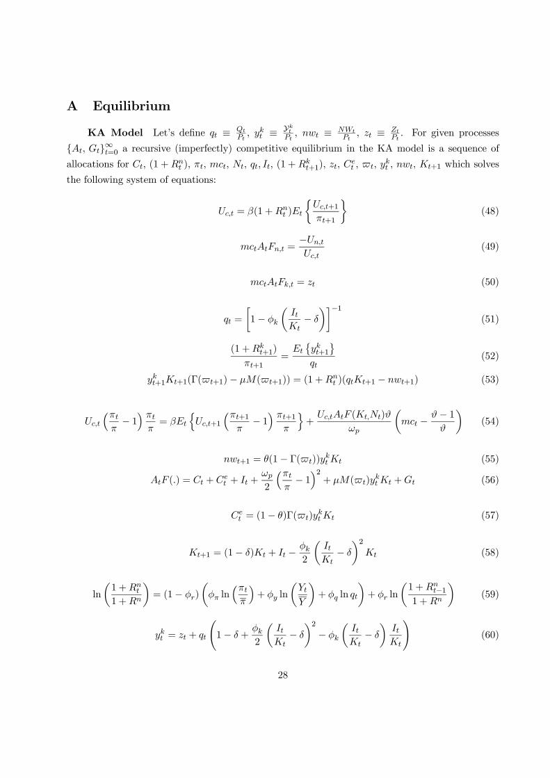
A Equilibrium

KA Model Let’s define qt ≡ Qt

Pt, ykt ≡ Ykt

Pt, nwt ≡ NWt

Pt, zt ≡ Zt

Pt. For given processes

At, Gt∞t=0 a recursive (imperfectly) competitive equilibrium in the KA model is a sequence of

allocations for Ct, (1 + Rnt ), πt, mct, Nt, qt, It, (1 +Rk

t+1), zt, Cet , t, y

kt , nwt, Kt+1 which solves

the following system of equations:

Uc,t = β(1 +Rnt )Et

½Uc,t+1

πt+1

¾(48)

mctAtFn,t =−Un,t

Uc,t(49)

mctAtFk,t = zt (50)

qt =

·1− φk

µItKt− δ

¶¸−1(51)

(1 +Rkt+1)

πt+1=

Et

©ykt+1

ªqt

(52)

ykt+1Kt+1(Γ( t+1)− µM( t+1)) = (1 +Rnt )(qtKt+1 − nwt+1) (53)

Uc,t

³πtπ− 1´ πtπ= βEt

nUc,t+1

³πt+1π− 1´ πt+1

π

o+

Uc,tAtF (Kt,Nt)ϑ

ωp

µmct − ϑ− 1

ϑ

¶(54)

nwt+1 = θ(1− Γ( t))yktKt (55)

AtF (.) = Ct + Cet + It +

ωp2

³πtπ− 1´2+ µM( t)y

ktKt +Gt (56)

Cet = (1− θ)Γ( t)y

ktKt (57)

Kt+1 = (1− δ)Kt + It − φk2

µItKt− δ

¶2Kt (58)

ln

µ1 +Rn

t

1 +Rn

¶= (1− φr)

µφπ ln

³πtπ

´+ φy ln

µYt

Y

¶+ φq ln qt

¶+ φr ln

µ1 +Rn

t−11 +Rn

¶(59)

ykt = zt + qt

Ã1− δ +

φk2

µItKt− δ

¶2− φk

µItKt− δ

¶ItKt

!(60)

28

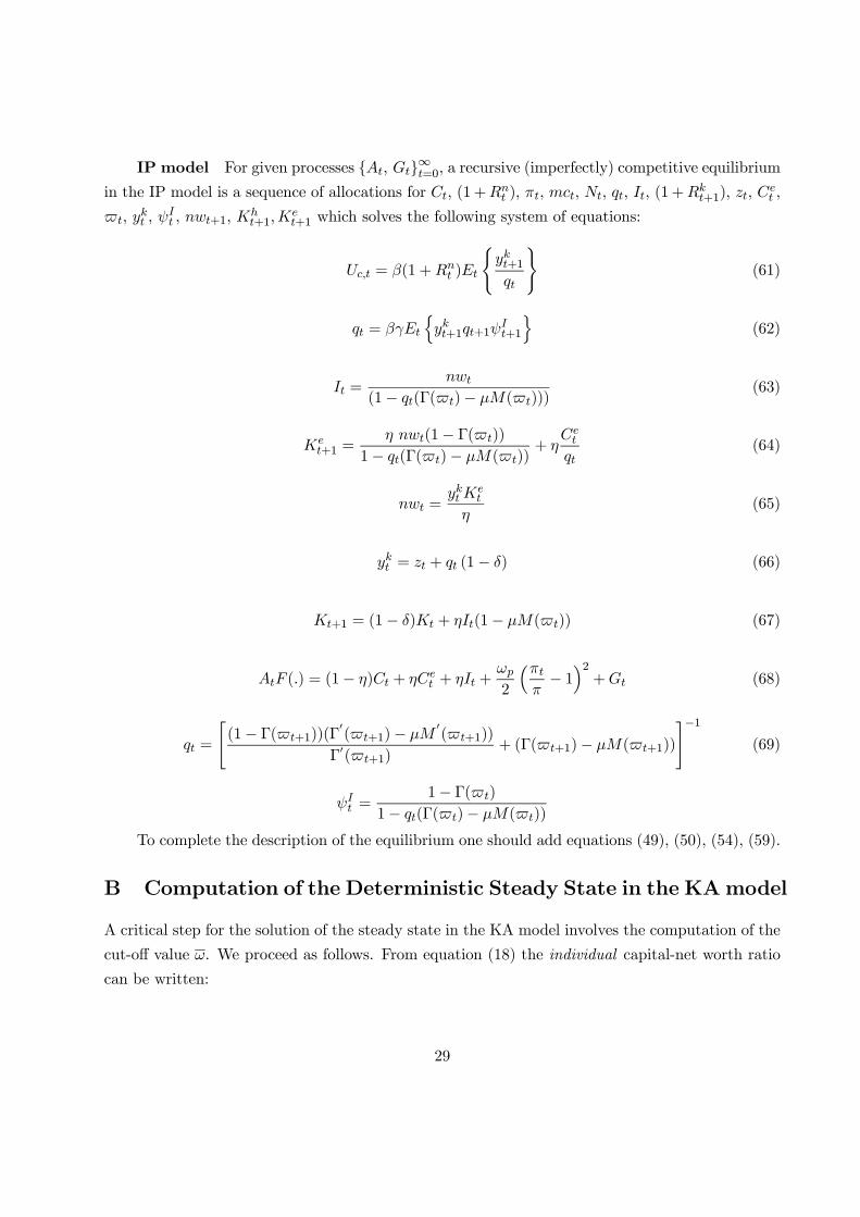
IP model For given processes At, Gt∞t=0, a recursive (imperfectly) competitive equilibriumin the IP model is a sequence of allocations for Ct, (1 +Rn

t ), πt, mct, Nt, qt, It, (1 +Rkt+1), zt, C

et ,

t, ykt , ψ

It , nwt+1, K

ht+1,K

et+1 which solves the following system of equations:

Uc,t = β(1 +Rnt )Et

(ykt+1qt

)(61)

qt = βγEt

nykt+1qt+1ψ

It+1

o(62)

It =nwt

(1− qt(Γ( t)− µM( t)))(63)

Ket+1 =

η nwt(1− Γ( t))

1− qt(Γ( t)− µM( t))+ η

Cet

qt(64)

nwt =yktK

et

η(65)

ykt = zt + qt (1− δ) (66)

Kt+1 = (1− δ)Kt + ηIt(1− µM( t)) (67)

AtF (.) = (1− η)Ct + ηCet + ηIt +

ωp2

³πtπ− 1´2+Gt (68)

qt =

"(1− Γ( t+1))(Γ

0( t+1)− µM

0( t+1))

Γ0( t+1)+ (Γ( t+1)− µM( t+1))

#−1(69)

ψIt =

1− Γ( t)

1− qt(Γ( t)− µM( t))

To complete the description of the equilibrium one should add equations (49), (50), (54), (59).

B Computation of the Deterministic Steady State in the KAmodel

A critical step for the solution of the steady state in the KA model involves the computation of the

cut-off value ω. We proceed as follows. From equation (18) the individual capital-net worth ratio

can be written:

29

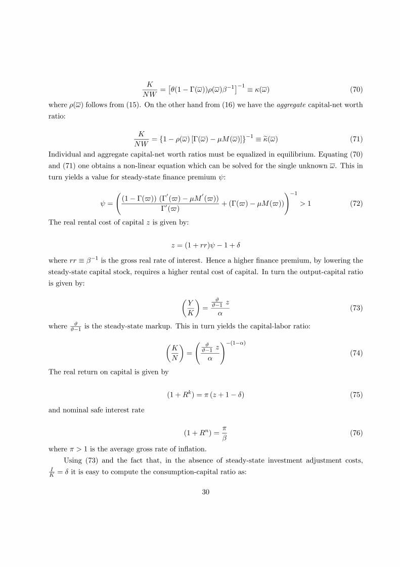
K

NW=£θ(1− Γ(ω))ρ(ω)β−1¤−1 ≡ κ(ω) (70)

where ρ(ω) follows from (15). On the other hand from (16) we have the aggregate capital-net worth

ratio:

K

NW= 1− ρ(ω) [Γ(ω)− µM(ω)]−1 ≡ eκ(ω) (71)

Individual and aggregate capital-net worth ratios must be equalized in equilibrium. Equating (70)

and (71) one obtains a non-linear equation which can be solved for the single unknown ω. This in

turn yields a value for steady-state finance premium ψ:

ψ =

Ã(1− Γ( )) (Γ

0( )− µM

0( ))

Γ0( )+ (Γ( )− µM( ))

!−1> 1 (72)

The real rental cost of capital z is given by:

z = (1 + rr)ψ − 1 + δ

where rr ≡ β−1 is the gross real rate of interest. Hence a higher finance premium, by lowering thesteady-state capital stock, requires a higher rental cost of capital. In turn the output-capital ratio

is given by:

µY

K

¶=

ϑϑ−1 z

α(73)

where ϑϑ−1 is the steady-state markup. This in turn yields the capital-labor ratio:

µK

N

¶=

Ãϑ

ϑ−1 z

α

!−(1−α)(74)

The real return on capital is given by

(1 +Rk) = π (z + 1− δ) (75)

and nominal safe interest rate

(1 +Rn) =π

β(76)

where π > 1 is the average gross rate of inflation.

Using (73) and the fact that, in the absence of steady-state investment adjustment costs,IK = δ it is easy to compute the consumption-capital ratio as:

30

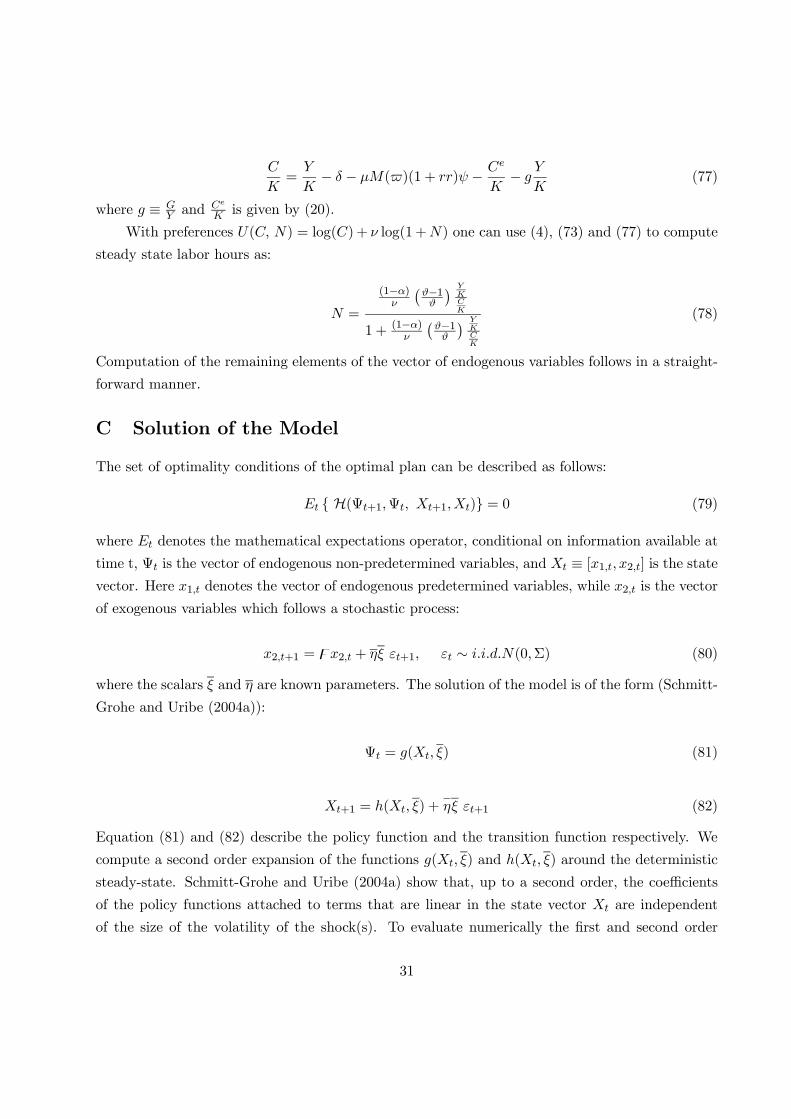
C

K=

Y

K− δ − µM( )(1 + rr)ψ − Ce

K− g

Y

K(77)

where g ≡ GY and Ce

K is given by (20).

With preferences U(C, N) = log(C) + ν log(1+N) one can use (4), (73) and (77) to compute

steady state labor hours as:

N =

(1−α)ν

¡ϑ−1ϑ

¢ YKCK

1 + (1−α)ν

¡ϑ−1ϑ

¢ YKCK

(78)

Computation of the remaining elements of the vector of endogenous variables follows in a straight-

forward manner.

C Solution of the Model

The set of optimality conditions of the optimal plan can be described as follows:

Et H(Ψt+1,Ψt, Xt+1,Xt) = 0 (79)

where Et denotes the mathematical expectations operator, conditional on information available at

time t, Ψt is the vector of endogenous non-predetermined variables, and Xt ≡ [x1,t, x2,t] is the statevector. Here x1,t denotes the vector of endogenous predetermined variables, while x2,t is the vector

of exogenous variables which follows a stochastic process:

x2,t+1 = zx2,t + ηξ εt+1, εt ∼ i.i.d.N(0,Σ) (80)

where the scalars ξ and η are known parameters. The solution of the model is of the form (Schmitt-

Grohe and Uribe (2004a)):

Ψt = g(Xt, ξ) (81)

Xt+1 = h(Xt, ξ) +−ηξ εt+1 (82)

Equation (81) and (82) describe the policy function and the transition function respectively. We

compute a second order expansion of the functions g(Xt, ξ) and h(Xt, ξ) around the deterministic

steady-state. Schmitt-Grohe and Uribe (2004a) show that, up to a second order, the coefficients

of the policy functions attached to terms that are linear in the state vector Xt are independent

of the size of the volatility of the shock(s). To evaluate numerically the first and second order

31

derivatives of the policy functions we employ the Matlab codes compiled by Schmitt-Grohe and

Uribe, available at the website http://www.econ.duke.edu/˜grohe. The second order expansion of

g and h is required for an accurate evaluation of the value of the variable W0 in the stochastic

steady state .

32

References

[1] Bernanke B., (2002), “Remarks by Governor Ben S. Bernanke Before the New York Chapter

of the National Association for Business Economics”, New York.

[2] Bernanke, B., M. Gertler, (2001),”Agency Costs, Net Worth and Business Fluctuations”,

American Economic Review, March, 14-31.

[3] Bernanke, B., M. Gertler, (2001), “Should Central Banks Respond to Movements in Asset

Prices?” American Economic Review Papers and Proceedings, 91 (2), 253-257.

[4] Bernanke, B., M. Gertler and S. Gilchrist, (1999), “The Financial Accelerator in a Quan-

titative Business Cycle Framework”, in J.B. Taylor, and M. Woodford, eds., Handbook of

Macroeconomics, Amsterdam: North-Holland.

[5] Carlstrom, C. and T. Fuerst (1997), “Agency Costs, Net Worth and Business Fluctuations: A

Computable General Equilibrium Analysis”, American Economic Review, 87, 893-910.

[6] Carlstrom, C. and T. Fuerst (1998), “Agency Costs and Business Cycles”, Economic Theory

12(3), 583-597.

[7] Cecchetti S., H. Genberg and S. Wadhwani (2002) ”Asset Prices in a Flexible Inflation Tar-

geting Framework”, NBER w.p # 8970.

[8] Chari V.V, P. Kehoe and E. McGrattan (2004), ”Business Cycle Accounting”, Federal Reserve

Bank of Minneapolis Staff Report, 328.

[9] Christiano, L. J. and Fisher, J. D. M., (2000), “Algorithms for solving dynamic models with

occasionally binding constraints,” Journal of Economic Dynamics and Control, vol. 24(8),

1179-1232, 7.

[10] Christiano L., M. Eichenbaum and C. Evans (2003), ”Nominal Rigidities and the Dynamic

Effects of a Shock to Monetary Policy, forthcoming Journal of Political Economy.

[11] Cook, D. (2002), ”Monetary Policy in Emerging Markets: Can Liability Dollarization Explain

Contractionary Devaluations”, forthcoming Journal of Monetary Economics.

[12] Detken, C. and F. Smets, (2004), ”Asset Price Booms and Monetary Policy”, ECB Working

Paper No. 364

[13] Dupor, B. (2003), ”Nominal Price versus Asset Price Stabilization”, mimeo Ohio State Uni-

versity.

33

[14] Erceg C., D. Henderson and A. Levin, (2000), “Optimal Monetary Policy with Staggered Wage

and Price Setting”, Journal of Monetary Economics, vol. 46, pp. 281-313.

[15] Gale, D. and M. Hellwig, (1985),“Incentive-Compatible Debt Contracts: The One-Period Prob-

lem”, Review of Economic Studies, 52, 647-663.

[16] Galı J., Lopez Salido D. and J. Valles (2003), ”Technology Shocks and Monetary Policy:

Assessing the Fed’s Performance” Journal of Monetary Economics, vol 50, 723-743.

[17] Gilchrist, S. and Leahy, J. V., (2002), “Monetary policy and asset prices”, Journal of Monetary

Economics, vol. 49(1), pages 75-97, 1.

[18] Iacoviello, M. (2004), ””House Prices, Borrowing Constraints and Monetary policy in the

Business Cycle” forthcoming American Economic Review.

[19] Ireland P.(2003), ”Endogenous Money or Sticky Prices”, Journal of Monetary Economics.

[20] Judd, K. (1998), ”Numerical Methods in Economics”, MIT Press.

[21] Khan, A., R. King and A.L. Wolman, (2003), “Optimal Monetary Policy”, Review of Economic

Studies, 60,4.

[22] Kim K.S., J. Kim, E. Schaumburg and C. Sims (2003), ”Calculating and Using Second Or-

der Accurate Solutions for Discrete Time Dynamic Equilibrium Models,” mimeo Brandeis

University.

[23] Kim K.S., J. Kim (2003), ”Spurious Welfare Reversals in International Business Cycle Models”,

Journal of International Economics 60, pp. 471-500.

[24] King R. and S. Rebelo, (1999), “Resuscitating Real Business Cycles,” in J.B. Taylor, and M.

Woodford, eds., Handbook of Macroeconomics, Amsterdam: North-Holland.

[25] King, R. and A. L. Wolman, (1999), “What Should the Monetary Authority Do When Prices

Are Sticky”, in Taylor, J. B., ed., Monetary Policy Rules, Chicago: university of Chicago

Press, 349-398.

[26] Kiyotaki, N. and J. Moore, (1997), “Credit Cycles”, Journal of Political Economy, 105, April

, 211-48.

[27] Kollmann R., (2003a), “Monetary Policy Rules in an Interdependent World”, CEPR DP 4012

34

[28] Kollmann R., (2003b), ”Welfare Maximizing Fiscal and Monetary Policy Rules”, mimeo Uni-

versity of Bonn.

[29] Kydland, F. and E. C. Prescott, (1980), “Dynamic Optimal Taxation, Rational Expectations

and Optimal Control”, Journal of Economic Dynamics and Control, 2:79-91.

[30] Lucas, R. E. and N. Stokey, (1983), “Optimal Fiscal and Monetary Policy in an Economy

Without Capital”, Journal of Monetary Economics, 12:55-93.

[31] Rotemberg, J. and M. Woodford, (1997), “An Optimization-Based Econometric Model for the

Evaluation of Monetary Policy”, NBER Macroeconomics Annual, 12: 297-346.

[32] Schmitt-Grohe S. and M. Uribe, (2003), ”Optimal, Simple, and Implementable Monetary and

Fiscal Rules”, mimeo Duke University.

[33] Schmitt-Grohe S. and M. Uribe, (2004a), ”Solving Dynamic General EquilibriumModels Using

a Second-Order Approximation to the Policy Function”, Journal of Economic Dynamics and

Control 28, 645-858.

[34] Schmitt-Grohe S. and M. Uribe, (2004b), “Optimal Operational Monetary Policy in the

Christiano-Eichenbaum-Evans Model of the U.S. Business Cycle ”, mimeo Duke University.

[35] Woodford, Michael (2003), Interest and Prices: Foundations of a Theory of Monetary Policy,

Princeton University Press..

35

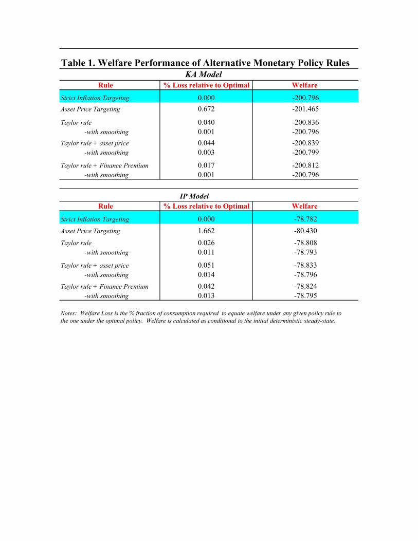
Table 1. Welfare Performance of Alternative Monetary Policy Rules KA Model

Rule % Loss relative to Optimal Welfare

Strict Inflation Targeting 0.000 -200.796Asset Price Targeting 0.672 -201.465

Taylor rule 0.040 -200.836 -with smoothing 0.001 -200.796Taylor rule + asset price 0.044 -200.839 -with smoothing 0.003 -200.799

Taylor rule + Finance Premium 0.017 -200.812 -with smoothing 0.001 -200.796

IP Model Rule % Loss relative to Optimal Welfare

Strict Inflation Targeting 0.000 -78.782Asset Price Targeting 1.662 -80.430Taylor rule 0.026 -78.808 -with smoothing 0.011 -78.793

Taylor rule + asset price 0.051 -78.833 -with smoothing 0.014 -78.796Taylor rule + Finance Premium 0.042 -78.824 -with smoothing 0.013 -78.795

Notes: Welfare Loss is the % fraction of consumption required to equate welfare under any given policy rule to the one under the optimal policy. Welfare is calculated as conditional to the initial deterministic steady-state.

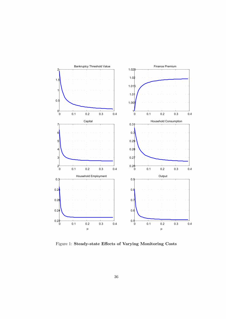
0 0.1 0.2 0.3 0.40

0.5

1

1.5

2Bankruptcy Threshold Value

0 0.1 0.2 0.3 0.41

1.005

1.01

1.015

1.02

1.025Finance Premium

0 0.1 0.2 0.3 0.42

3

4

5

6

7Capital

0 0.1 0.2 0.3 0.40.26

0.27

0.28

0.29

0.3

0.31Household Consumption

0 0.1 0.2 0.3 0.40.22

0.24

0.26

0.28

0.3Household Employment

0 0.1 0.2 0.3 0.40.5

0.6

0.7

0.8

0.9Output

µµ

Figure 1: Steady-state Effects of Varying Monitoring Costs

36

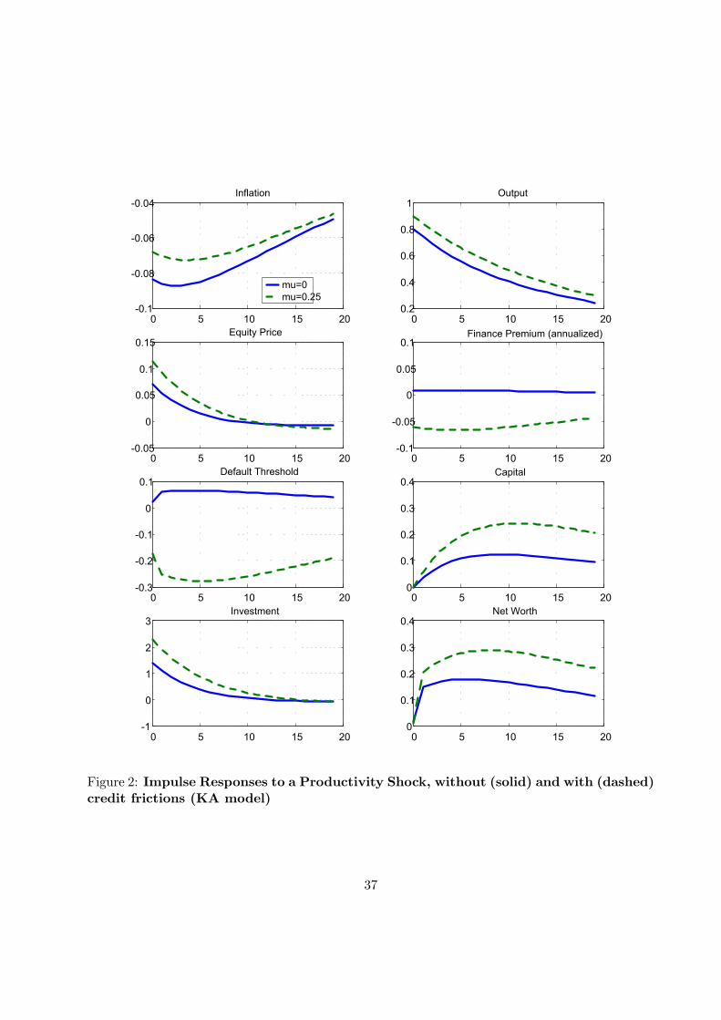
0 5 10 15 20-0.1

-0.08

-0.06

-0.04Inflation

0 5 10 15 200.2

0.4

0.6

0.8

1Output

0 5 10 15 20-0.05

0

0.05

0.1

0.15Equity Price

0 5 10 15 20-0.1

-0.05

0

0.05

0.1Finance Premium (annualized)

0 5 10 15 20-0.3

-0.2

-0.1

0

0.1Default Threshold

0 5 10 15 200

0.1

0.2

0.3

0.4Capital

0 5 10 15 20-1

0

1

2

3Investment

0 5 10 15 200

0.1

0.2

0.3

0.4Net Worth

mu=0mu=0.25

Figure 2: Impulse Responses to a Productivity Shock, without (solid) and with (dashed)credit frictions (KA model)

37

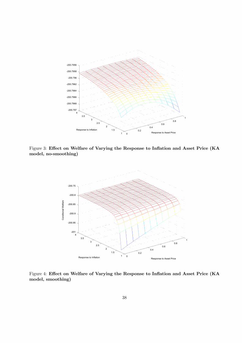
00.2

0.40.6

0.81

11.5

22.5

33.5

4-200.797

-200.7968

-200.7966

-200.7964

-200.7962

-200.796

-200.7958

-200.7956

Response to Asset PriceResponse to Inflation

Figure 3: Effect on Welfare of Varying the Response to Inflation and Asset Price (KAmodel, no-smoothing)

00.2

0.40.6

0.81

11.5

22.5

33.5

4-201

-200.95

-200.9

-200.85

-200.8

-200.75

Response to Asset PriceResponse to Inflation

Con

ditio

nal W

elfa

re

Figure 4: Effect on Welfare of Varying the Response to Inflation and Asset Price (KAmodel, smoothing)

38

-1

-0.5

0

0.5

1

1

1.5

2

2.5

3-201.15

-201.1

-201.05

-201

-200.95

-200.9

-200.85

-200.8

-200.75

-200.7

Response to Finance PremiumResponse to Inflation

Con

ditio

nal W

elfa

re

Figure 5: Effect on Welfare of Varying the Response to Inflation and Finance Premium(KA model, no-smoothing)

-1

-0.5

0

0.5

1

1

1.5

2

2.5

3-200.7995

-200.799

-200.7985

-200.798

-200.7975

-200.797

-200.7965

-200.796

-200.7955

Response to Finance PremiumResponse to Inflation

Con

ditio

nal W

elfa

re

Figure 6: Effect on Welfare of Varying the Response to Inflation and Finance Premium(KA model, smoothing)

39

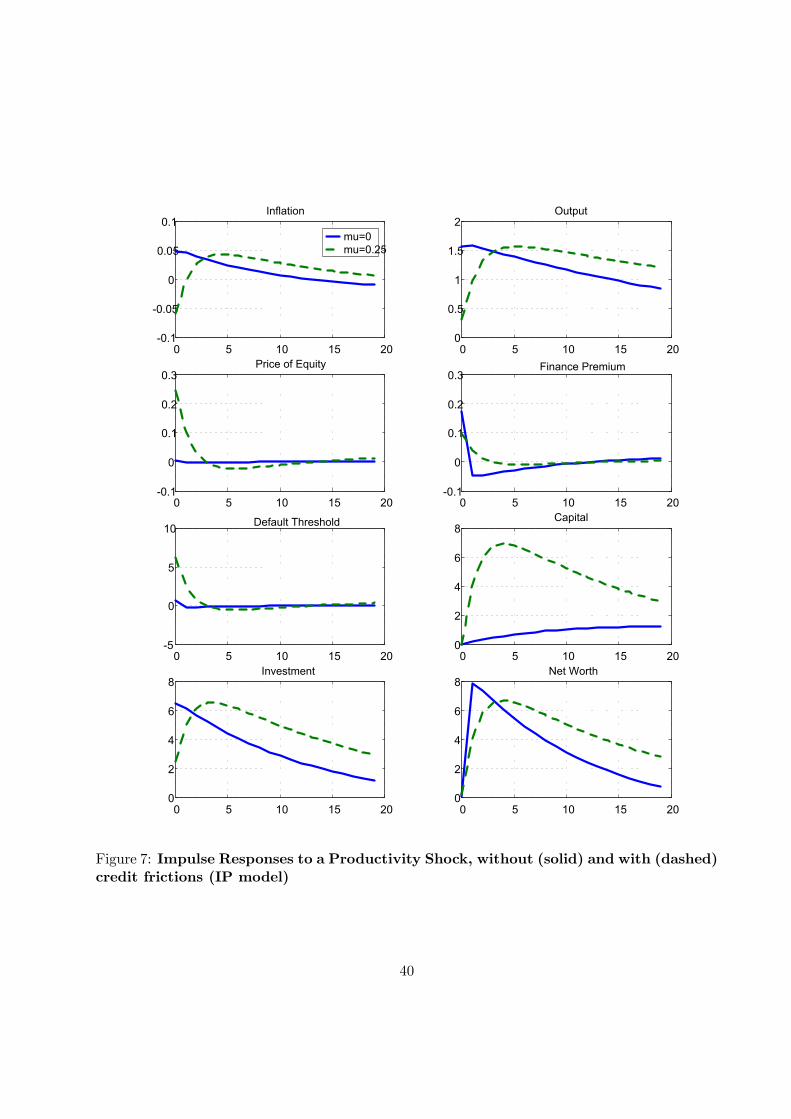
0 5 10 15 20-0.1

-0.05

0

0.05

0.1Inflation

0 5 10 15 200

0.5

1

1.5

2Output

0 5 10 15 20-0.1

0

0.1

0.2

0.3Price of Equity

0 5 10 15 20-0.1

0

0.1

0.2

0.3Finance Premium

0 5 10 15 20-5

0

5

10 Default Threshold

0 5 10 15 200

2

4

6

8Capital

0 5 10 15 200

2

4

6

8Investment

0 5 10 15 200

2

4

6

8Net Worth

mu=0mu=0.25

Figure 7: Impulse Responses to a Productivity Shock, without (solid) and with (dashed)credit frictions (IP model)

40

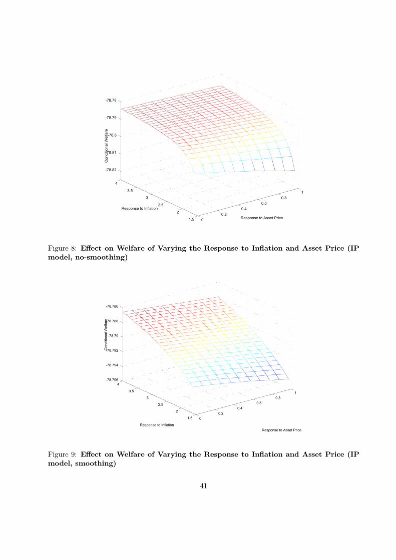
00.2

0.40.6

0.81

1.5

2

2.5

3

3.5

4

-78.82

-78.81

-78.8

-78.79

-78.78

Response to Asset Price

Response to Inflation

Con

ditio

nal W

elfa

re

Figure 8: Effect on Welfare of Varying the Response to Inflation and Asset Price (IPmodel, no-smoothing)

00.2

0.40.6

0.81

1.5

2

2.5

3

3.5

4-78.796

-78.794

-78.792

-78.79

-78.788

-78.786

Response to Asset PriceResponse to Inflation

Con

ditio

nal W

elfa

re

Figure 9: Effect on Welfare of Varying the Response to Inflation and Asset Price (IPmodel, smoothing)

41