The Optimal Monetary Response to a Financial CrisisPreliminary and Incomplete

Fabio Braggion ∗ Lawrence J. Christiano† Jorge Roldos‡

January 30, 2005§.

Abstract

We describe a model in which the optimal monetary policy response to a financial crisis is to raisethe interest rate immediately, and then reduce it sharply. This pattern is consistent with what actuallyhappened in the Asian crisis episodes.

1 Introduction

The Asian financial crises of 1997-98 triggered a sharp debate over the appropriate response of policy to a

financial crises. The hallmark of the crises was a “sudden stop” (Calvo, 1998): capital inflows turned into

outflows and output suddenly collapsed. Some argued that the monetary authorities should raise interest

rates, to help reverse the outflow of capital. Others argued interest rates should be cut to stimulate output.

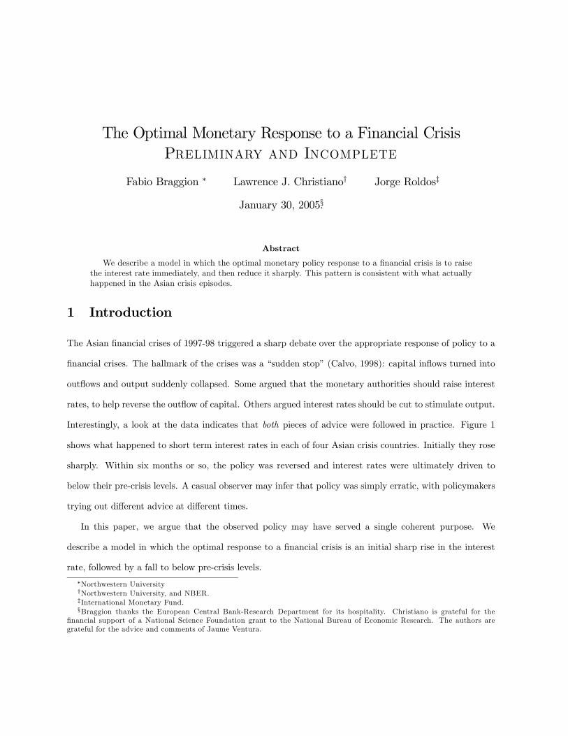
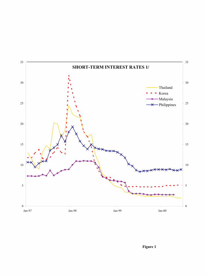
Interestingly, a look at the data indicates that both pieces of advice were followed in practice. Figure 1

shows what happened to short term interest rates in each of four Asian crisis countries. Initially they rose

sharply. Within six months or so, the policy was reversed and interest rates were ultimately driven to

below their pre-crisis levels. A casual observer may infer that policy was simply erratic, with policymakers

trying out different advice at different times.

In this paper, we argue that the observed policy may have served a single coherent purpose. We

describe a model in which the optimal response to a financial crisis is an initial sharp rise in the interest

rate, followed by a fall to below pre-crisis levels.

∗Northwestern University†Northwestern University, and NBER.‡International Monetary Fund.§Braggion thanks the European Central Bank-Research Department for its hospitality. Christiano is grateful for the

financial support of a National Science Foundation grant to the National Bureau of Economic Research. The authors aregrateful for the advice and comments of Jaume Ventura.

Our finding builds on the analysis of Christiano, Gust and Roldos (2004) (CGR). CGR study the

conditions under which an interest rate cut would stimulate output, employment and raise welfare in the

midst of a financial crisis of this kind. In their model, firms require domestic currency working capital to

hire labor and foreign currency working capital to finance an imported intermediate input. They adopt the

asset market frictions formalized in the limited participation models (Lucas 1990, Fuerst 1992, Christiano

and Eichenbaum, 1992, 1995), and model a financial crisis as a time in which collateral constraints are

suddenly tightened. The authors show that when these financial frictions are combined with real frictions

in the reallocation of labor across sectors, a cut in interest rates is most likely to result in a welfare-reducing

fall in output and employment. When these real frictions are absent, a cut in interest rates improves asset

values and promotes a welfare-improving economic expansion.

In this paper we extend the work in CGR in three dimensions. First, we provide empirical evidence

to support the main assumptions of the model, namely, the role of collateral constraints and imported

inputs in the collapse in output and as constraints to the conduct of monetary policy during this kind of

financial crisis. Second, we combine the production technology in the two examples of CGR into a unified

technology where labor is immobile in the short-run but can be reallocated across sectors in the medium

run.1 Third, we study what the optimal monetary policy would be in such an environment.2 Fourth, we

present a simple example that sheds light on a core feature of our dynamic model that may at first seem

highly counterintuitive: the fact that an interest rate rise raises employment and utility. In the dynamic

model, an increase in the interest rate introduces a distortion in the labor market. Normally, this can be

expected to reduce employment and utility. Our simple example is non-monetary and there is only one

period. The effects of the interest rate in the dynamic model are captured with a straight tax on labor.

1A similar friction is used by Fernandez de Cordoba and Kehoe (2001) to study the role of capital flows following Spain’sentry to the European Community.

2Other studies have examined the relationship between optimal interest rates and financial crises. Aghion, Bacchetta andBanerjee (2000) present a model with multiple equilibria, in which a currency crisis is the bad equilibrium. The possibilityof the bad equilibrium is due to the interplay between the credit constraints on private firms and the existence of nominalprice rigidities. The authors show that the monetary authority should tighten monetary policy after any shock that resultsin the possibility of the currency crisis equilibrium. Our analysis differs from this analysis in three ways. First, equilibriummultiplicity does not play a role in our analysis. Second, our model emphasizes a different set of rigidities. Third, Aghion,Bacchetta and Banerjee focus on the prevention of crises, while we focus on their management after they occur. Similarly,Caballero and Krishnamurthy (2002) show that when the economy faces a binding international collateral constraint, amonetary expansion that would redistribute funds from consumers to distressed firms has no real effects. Given this lack ofeffectiveness, a monetary authority that trades-off output and an inflation target focuses on the latter and tightens monetarypolicy to achieve the inflation objective.

1

Although a rise in the tax rate distorts the labor market, the overall effects are welfare improving because

the collateral constraint on international loans becomes less binding.

The paper is organized as follows. In the first section we provide empirical evidence on the role

of collateral constraints and imported intermediate inputs and describe the objectives, constraints and

outcomes of monetary policy in the Asian crises countries. The second section presents the simple example.

The third section presents our dynamic, monetary model and we highlight its primary financial and real

frictions. Section 4 discusses model calibration and section 5 we present the main results. There is a final,

concluding section.

2 Collateral Constraints and Monetary Policy

In this section, we provide empirical evidence that motivates and supports some of the key assumptions in

our model, as well as the objective, constraints and final outcomes of monetary policy in recent emerging

market crises.

The assumption that the land and capital of the firm is collateral for international loans plays an impor-

tant role in our analysis. We recognize the enforcement problems and other financial market imperfections

that are pervasive in emerging markets hence do not restrict ourselves to a narrow (legal or contractual)

view of collateral. Rather, we see collateral constraints as capturing the tightening of credit conditions and

associated balance sheet problems seen in the aftermath of a financial crisis. They do not just reflect the

insistence by creditors that collateral be written explicitly into loan contracts, but also the possibility that

regulators induce banks to invest only in ‘secure’ loans, loans to companies that have ample assets in the

event that things go wrong. We now briefly provide some empirical evidence on the use of collateral in

loan markets.

The use of collateral in loan markets is widespread. Berger and Udell (1990) document that around 70

percent of commercial and industrial loans in the US are secured and Black, De Meza and Jeffreys report

similar evidence for the UK. In emerging markets, Gelos and Werner (1999) report that around 60 percent

of loans are collateralized in Mexico, while survey evidence from the Bank of Thailand put the figure at

more than 80 percent for that country. A review of financial conditions of the Asian crises countries (IMF

2

1999) notes that lending against collateral was a widespread practice also in these countries.

There is also ample evidence that collateral practices are procyclical. Asea and Blomberg (1998) provide

evidence that bank lending standards vary over the US business cycle: in an average contraction, the degree

of loan collateralization and spreads charged over Treasuries increase over the year before the trough. In

an interesting paper on the recent emerging market crises, Edison, Luangaram and Miller (2000) report

that Thai banks that used to lend up to 70-80 percent of the value of pledged collateral before the crisis,

moved to lend up to just 50-60 percent after the crisis. More important for our paper, the fraction of

syndicated loans in international markets that is collateralized reached a peak (at 42 percent of the total;

see Table 1) in the year of the Asian crises. This is reinforced by the fact that the level of syndicated loans

also peaked in 1997, in line with the finding in Chadha and Folkerts-Landau (2000) that suggests that

commercial banks appear to be lenders of “second-to-last resort” in international credit markets.

There is, however, substantial debate on what constitutes international collateral. In a recent paper,

Caballero and Krishnamurthy (2000) assume (with some caveats) that only a fraction of the assets used in

the tradable sector would be accepted as collateral by foreign creditors, whereas the totality of domestic

assets would be accepted as domestic collateral. Inadequate amounts of international collateral and im-

perfect aggregation of domestic collateral are shown to lead to fire sales of domestic assets and financial

crises.

In recognition of the difficulties defining what constitutes international collateral and the different

institutional arrangements and credit market imperfections that characterize emerging markets, we consider

the following simplified collateral constraint expressed in units of the foreign currency:

Q

SK ≥ R∗z +B.

B indicates the stock of long-term external debt; z represents short-term external borrowing to finance a

foreign intermediate input; R∗ corresponds to the associated interest rate; K stands for domestic physical

assets like land and capital; Q is the value (in domestic currency units) of a unit of K; and S is the nominal

exchange rate. We assume that under regular conditions, the collateral constraint is not binding, while it

suddenly binds with the onset of a crisis. This may be because in normal times, output in addition to land

and capital is acceptable as collateral. We suppose that a crisis is a time when international loans must be

3

collateralized by physical assets such as land and capital, and that this restriction is binding. Alternatively,

in a crisis the fraction of domestic assets accepted as collateral by foreigners suddenly falls.3 In any case, in

our analysis we model the imposition of a binding collateral constraint as an exogenous, unforeseen event.4

The collateral constraint in this paper provides a financial friction that captures in a natural way the

“balance sheet” effects frequently mentioned in the discussion of recent crises. A number of recent papers

(including Krugman (1999), Aghion, Bacchetta and Banerjee (2000), Caballero and Krishnamurthy (2000,

2002), Cespedes, Chang and Velasco (2000), Gertler, Gilchrist and Natalucci (2000), Mendoza and Smith

(2002)) introduce credit constraints that capture some aspects of the balance sheet channel. However, while

these papers incorporate the adverse effects derived from the existence of foreign currency denominated

debts, the credit frictions in those papers constrain borrowing to be a fraction of current income—rather

than the current value of physical assets.5 The mismatch between assets and liabilities that underscored

the financial vulnerability of the crises countries is captured in our model by the fact that a large fraction

of domestic assets are in the nontraded sector while a relatively large fraction of liabilities are denominated

in terms of the traded good. Hence, a large and persistent fall in the relative price of nontraded goods

(ie. a real exchange rate depreciation) results in a fall in the value of assets relative to liabilities that

endogenously magnifies the tightening of credit conditions derived from the initial imposition of collateral

constraints in the aftermath of the crisis. In other words, our economy is capable of displaying a “sudden

stop” in capital inflows (Calvo, 1998, 2002) that is associated with large and persistent falls in output and

3The imposition of collateral constraints is also consistent with recent models of financial crises that focus on the role ofguarantees and moral hazard as causes of emerging markets crises (such as Krugman, 1999, Corsetti, Pesenti and Roubini,1998, Dooley, 1998, and Burnside, Eichenbaum and Rebelo, 2000). In fact, we should stress that our model does not attemptto model the causes of the financial crises but its effects on credit conditions. Now after a crisis happens, i.e. after theguarantees are exercised, the only way in which foreigners would extend further credit to a country would be under furtherguarantees or additional collateral. This additional collateral has been seen in explicit private (syndicated loan) contracts, inthe tightening of bank regulations that impose directly or indirectly collateral requirements, and in governments’ interventionand sales of distressed assets.

4 In some respects our framework resembles a reduced form representation of the environment considered in Albuquerqueand Hopenhayn (1997) and further developed in Cooley, Marimon and Quadrini (2001) and Monge (2001). There, aninvestment project requires an initial fixed investment, followed by a sequence of expenditures to make the investment projectproductive. The papers in this literature derive the optimal dynamic contract between the entrepreneur and a bank, as wellas a sequential decentralization. In the latter, the initial fixed investment is financed by long term debt that resembles our B,and the sequence of expenditures is financed by working capital loans with the entrepreneur being restricted by a collateralconstraint that resembles the one we adopt. This literature suggests a variety of factors that could cause collateral constraintsto suddenly become binding. For example, if there is a shock that causes the court system to be overwhelmed by bankruptcyfilings and other business in a recession, collateral constraints could suddenly bind because lenders now understand that thedefault option is more attractive to the marginal entrepreneur who wishes to borrow.

5A notable exception is Gertler, Gilchrist and Natalucci (2000), but the nature of the credit constraint is different from theone in this paper. Moreover, the current account is always zero in that paper, hence missing the connection between capitalflows and asset prices observed in the crises episodes.

4

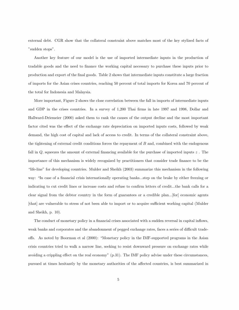
external debt. CGR show that the collateral constraint above matches most of the key stylized facts of

”sudden stops”.

Another key feature of our model is the use of imported intermediate inputs in the production of

tradable goods and the need to finance the working capital necessary to purchase these inputs prior to

production and export of the final goods. Table 2 shows that intermediate inputs constitute a large fraction

of imports for the Asian crises countries, reaching 50 percent of total imports for Korea and 70 percent of

the total for Indonesia and Malaysia.

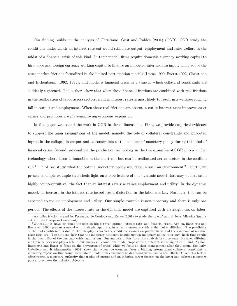
More important, Figure 2 shows the close correlation between the fall in imports of intermediate inputs

and GDP in the crises countries. In a survey of 1,200 Thai firms in late 1997 and 1998, Dollar and

Hallward-Driemeier (2000) asked them to rank the causes of the output decline and the most important

factor cited was the effect of the exchange rate depreciation on imported inputs costs, followed by weak

demand, the high cost of capital and lack of access to credit. In terms of the collateral constraint above,

the tightening of external credit conditions forces the repayment of B and, combined with the endogenous

fall in Q, squeezes the amount of external financing available for the purchase of imported inputs z . The

importance of this mechanism is widely recognized by practitioners that consider trade finance to be the

“life-line” for developing countries. Mulder and Sheikh (2003) summarize this mechanism in the following

way: “In case of a financial crisis internationally operating banks...step on the brake by either freezing or

indicating to cut credit lines or increase costs and refuse to confirm letters of credit...the bank calls for a

clear signal from the debtor country in the form of guarantees or a credible plan...[for] economic agents

[that] are vulnerable to stress of not been able to import or to acquire sufficient working capital (Mulder

and Sheikh, p. 10).

The conduct of monetary policy in a financial crises associated with a sudden reversal in capital inflows,

weak banks and corporates and the abandonment of pegged exchange rates, faces a series of difficult trade-

offs. As noted by Boorman et al (2000): “Monetary policy in the IMF-supported programs in the Asian

crisis countries tried to walk a narrow line, seeking to resist downward pressure on exchange rates while

avoiding a crippling effect on the real economy” (p.31). The IMF policy advise under these circumstances,

pursued at times hesitantly by the monetary authorities of the affected countries, is best summarized in

5

Mussa (2000, p2): “Indeed, in January 1998, the currencies of these five countries had lost more than half

their values in terms of the US dollar. In this situation, the IMF’s policy advise, in all cases, was that

short-term interest rates needed to be raised significantly (and temporarily)...it was recognized, of course,

that significant increases in short-term interest rates, even if pursued for relatively brief periods, had

negative side effects for economic activity and for the financial conditions of both nonfinancial businesses

and financial institutions. This was likely to be especially true in Asian countries where there was a high

degree of leverage in the economy. On the other hand, for those countries with substantial net indebtedness

in foreign currencies, there were costs and risks of systemic disruption from allowing uncontrolled exchange

rate depreciation.” The trade-off between high interest rates and a highly depreciated currency depends

critically on the balance sheet exposures of corporates and financial institutions, and accurate estimates of

such balance sheet positions are very hard to come by.6

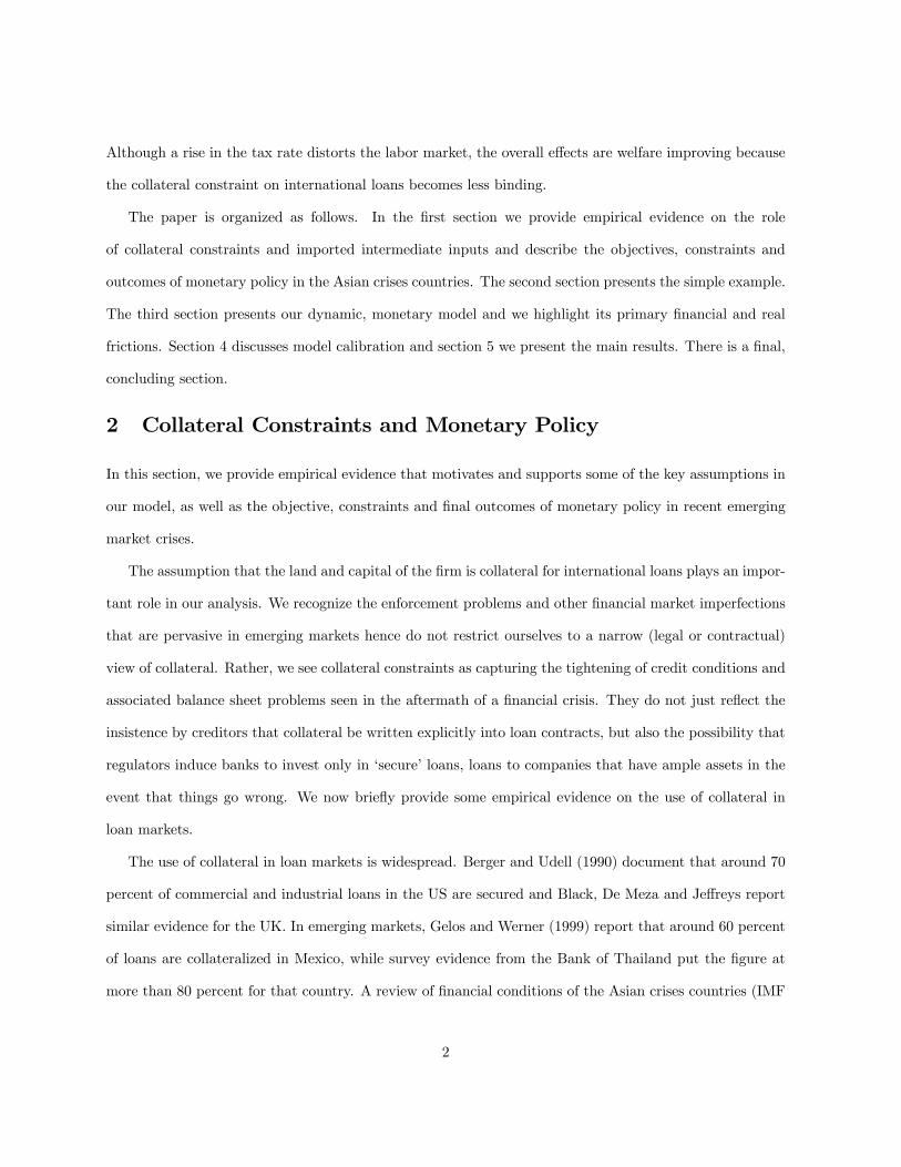
In the event, short-term nominal interest rates were increased substantially in the first half of 1998.

Interest rates were around 12 percent in the period before the crises and spiked at level of 25-30 percent in

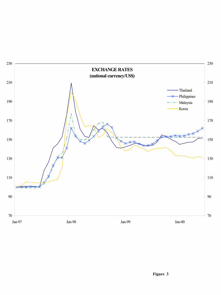
early January 1998.7 Exchange rates peaked at pretty much the same time and then appreciated steady

(see Figure 3). Interest rates remained high for a while but started to come down once exchange rates

stabilized and other elements of the crisis management packages—including roll-overs and additional external

financing—were in place. Interest rates reached pre-crises level by mid-1998 and continued to fall to levels

between 2 and 5 percent per year.

Berg et al. (2003) document the fact that monetary policy in countries that experienced currency crises

generally went through two phases: an initial chaotic period of crises containment—basically what we just

described—and a longer period during which the monetary policy framework and institutions were more

fully developed. Before the crises, the Asian countries had followed relatively loose monetary and credit

6Claessens, Djankov and Ferri (1998) assess the ex-post impact of the currency and interest rate shocks on the solvencyof a sample of East Asian firms between early 1997 and 1998. They find that the exchange rate shock alone was sufficientto drive almost two-thirds of Indonesian firms, 20 percent of Korean firms and 10 percent of Thai firms in their sample intoinsolvency. The effect of interest rate increases was smaller, driving about 2-5 percent of firms in each of the countries intoinsolvency. This suggests that the trade-off was somewhat tilted towards resisting an ”excessive” exchange rate depreciation.

7Malaysia’s short-term interest rates were increased less than in the other countries—but overnight rates rose from 6 percentin June 1997 to 35 percent in July 1997. Analysts attribute this difference to the lower exposure to exchange rate risks andrelatively higher domestic leverage of Malaysian corporates and financial institutions. Also, the authorities tightened monetaryconditions through various direct instruments such as credit plans for financial institutions and a ban on new lending to theproperty sector (see Boorman et al, 2000).

6

policies. Following the initial increase in interest rates aimed at stabilizing exchange rates, most countries

moved to avoid a an inflation/depreciation spiral and continued to float while improving monetary control.8

Indeed, the authors show that the countries that most quickly regained monetary control tended to have

the smallest output declines and have brought inflation down relatively fast.9

3 Example

A basic result in the dynamic simulations reported later on is that a rise in the domestic interest rate can

produce a rise in equilibrium employment when there is a binding collateral constraint. At first glance this

result may seem puzzling since in effect the rise in the interest rate introduces a distortion in the labor

market. Partial equilibrium reasoning suggests this distortion should lead to a decrease in employment, not

an increase. In fact, the partial equilibrium effect may be overwhelmed by a particular general equilibrium

effect when there is a binding collateral constraint. We illustrate this point with sharply simplified version

of our dynamic monetary model.

Our example has one period only. The economy has a traded good sector and a non-traded good sector.

The non-traded good sector uses labor and no imported intermediate inputs, while the traded sector uses no

labor and an imported intermediate input. Financing for the imported intermediate input must be obtained

at the beginning of the period, subject to a binding collateral constraint. International loans are paid off at

the end of the period. The collateral used in the international loans are productive in the nontraded good

sector. When the labor tax rate is increased, this raises the marginal cost of non-traded goods and leads

to a rise in their relative price. This rise in price increases the value of the collateral in the non-traded

good sector and permits an expansion in imports of the intermediate good. The increased imports leads to

an increased demand for the non-traded good, because traded and non-traded goods are complementary

in the production of a final good. Through this sequence of events, the net effect of the rise in the labor

tax rate is to increase employment and utility. In effect, the binding collateral constraint represents an

8Berg et al. (2003) note that two pre-requisites are necessary to regain monetary stability: the first is the elimination ofdollar shortages and the second the resolution of banking sector problems. The first phase was longer in Indonesia—because ofthe longer period involved in resolving banking problems—and in Mexico—because of doubts about the resolution of the dollarliquidity and banking problems.

9 In the case of Korea, inflation was very low—under 1 percent in the year after the crisis—despite a large nominal depreciationof the won. Burnstein, Eichenbaum, and Rebelo (2002) explain this in terms of relatively large component of nontradabledistribution costs in the final consumption of tradable goods.

7

inefficiency wedge for the economy. By introducing an inefficiency wedge in the labor market, the labor

tax rate helps mitigate the effects of the inefficiency wedge associated with the collateral constraint. The

overall effect is welfare-improving.

3.1 Model

A representative household has preferences over consumption and labor, c and L, as follows:

u(c, L) = c− ψ01 + ψ

L1+ψ. (1)

The non-tradeable consumption good is produced using traded and non-traded intermediate goods using

the following Leontief technology:

c = min©(1− γ)cT , γcN

ª. (2)

Traded and non-traded intermediate goods are produced, respectively, using the following two technologies:

yT = Azθ, yN = KαL1−α. (3)

Here, z is a good which is imported from abroad, and yT is the gross amount of traded goods produced.

Traded goods are used in domestic production, and for paying international debt as follows:

yT = cT +R∗z, (4)

where R∗ is the gross rate of interest, in traded good terms. In (4), z is the amount borrowed from abroad

to finance the purchase of z for use in (3), so that R∗z is the total quantity of traded goods owed to foreign

creditors at the end of the period. Equation (4) is the market clearing condition in the market for traded

goods. Non-traded goods can only be used as intermediate goods in production of c, so that:

yN = cN .

We consider a competitive market environment. The representative household maximizes utility, (1),

subject to the budget constraint,

pc ≤ wL+ π + T.

8

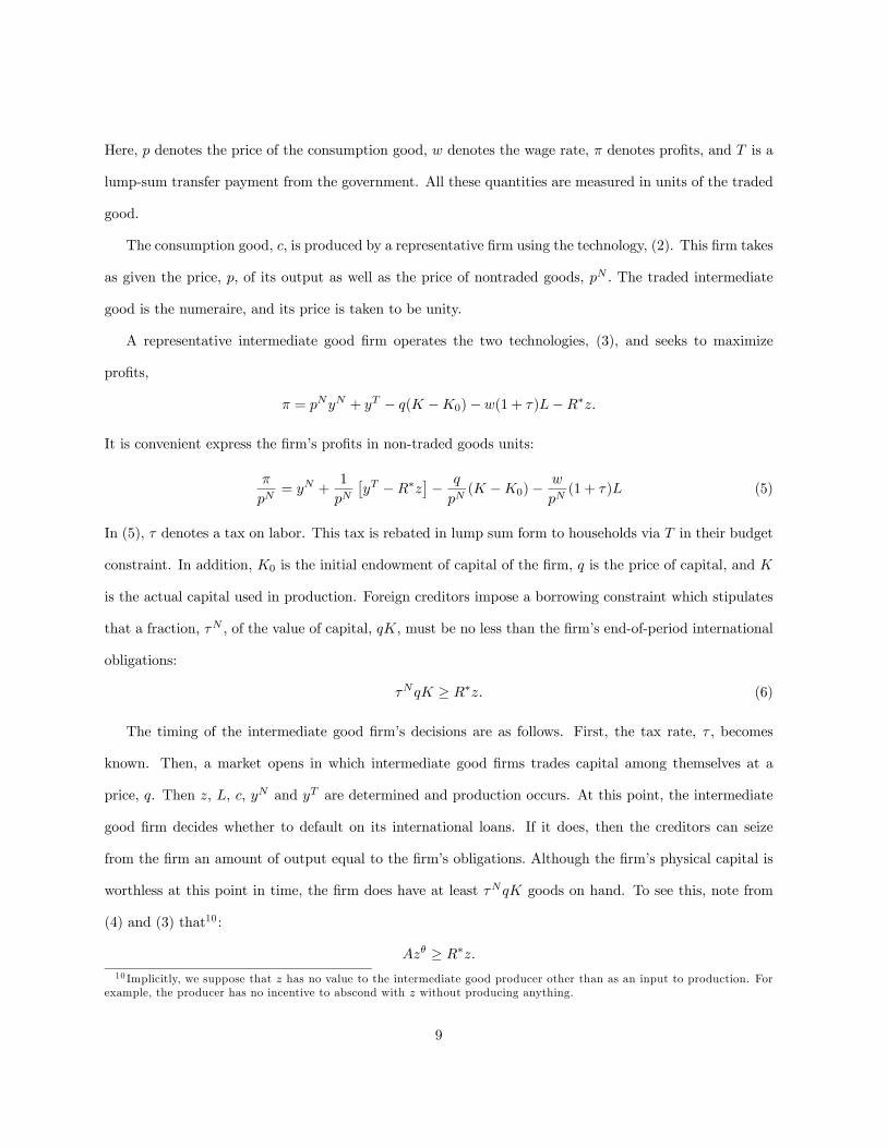
Here, p denotes the price of the consumption good, w denotes the wage rate, π denotes profits, and T is a

lump-sum transfer payment from the government. All these quantities are measured in units of the traded

good.

The consumption good, c, is produced by a representative firm using the technology, (2). This firm takes

as given the price, p, of its output as well as the price of nontraded goods, pN . The traded intermediate

good is the numeraire, and its price is taken to be unity.

A representative intermediate good firm operates the two technologies, (3), and seeks to maximize

profits,

π = pNyN + yT − q(K −K0)− w(1 + τ)L−R∗z.

It is convenient express the firm’s profits in non-traded goods units:

π

pN= yN +

1

pN£yT −R∗z

¤− q

pN(K −K0)−

w

pN(1 + τ)L (5)

In (5), τ denotes a tax on labor. This tax is rebated in lump sum form to households via T in their budget

constraint. In addition, K0 is the initial endowment of capital of the firm, q is the price of capital, and K

is the actual capital used in production. Foreign creditors impose a borrowing constraint which stipulates

that a fraction, τN , of the value of capital, qK, must be no less than the firm’s end-of-period international

obligations:

τNqK ≥ R∗z. (6)

The timing of the intermediate good firm’s decisions are as follows. First, the tax rate, τ , becomes

known. Then, a market opens in which intermediate good firms trades capital among themselves at a

price, q. Then z, L, c, yN and yT are determined and production occurs. At this point, the intermediate

good firm decides whether to default on its international loans. If it does, then the creditors can seize

from the firm an amount of output equal to the firm’s obligations. Although the firm’s physical capital is

worthless at this point in time, the firm does have at least τNqK goods on hand. To see this, note from

(4) and (3) that10 :

Azθ ≥ R∗z.

10 Implicitly, we suppose that z has no value to the intermediate good producer other than as an input to production. Forexample, the producer has no incentive to abscond with z without producing anything.

9

As a result, the profits of a firm which pays labor in the non-traded good sector, but contemplates not

repaying its international debt are:

αpNyN +Azθ ≥ R∗z.

A competitive equilibrium is a set of allocations and prices where households and firms solve their

problems subject to their constraints and markets clear.

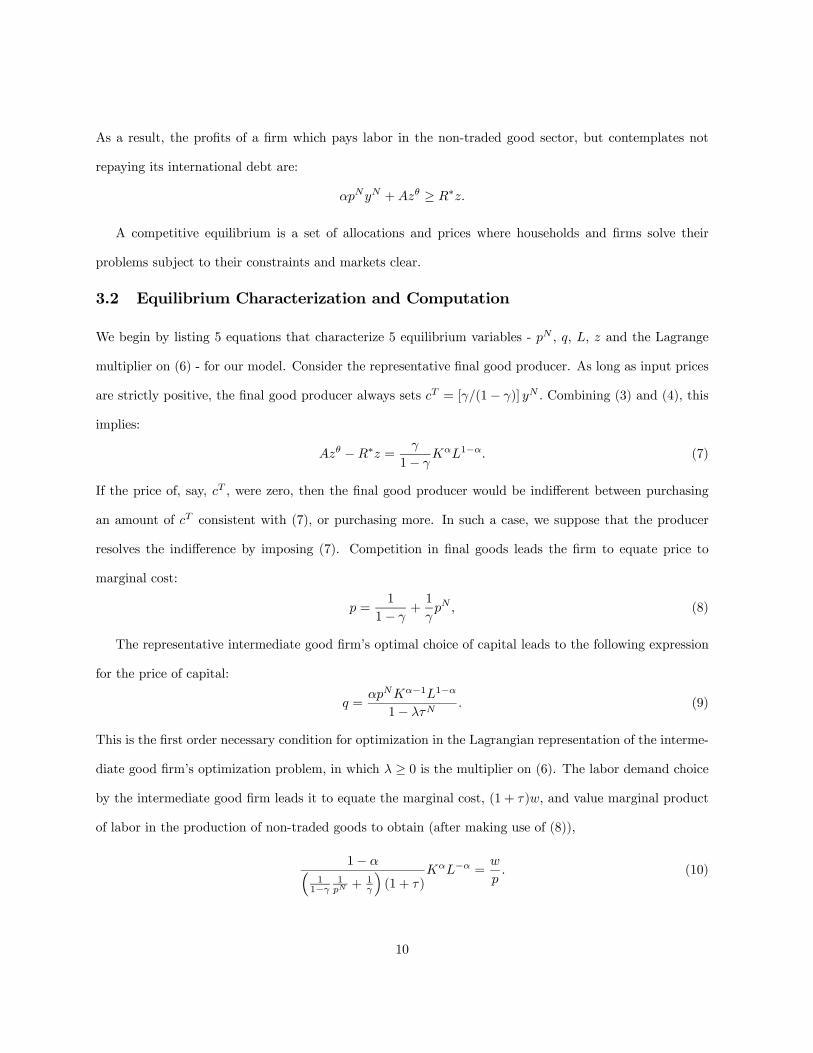
3.2 Equilibrium Characterization and Computation

We begin by listing 5 equations that characterize 5 equilibrium variables - pN , q, L, z and the Lagrange

multiplier on (6) - for our model. Consider the representative final good producer. As long as input prices

are strictly positive, the final good producer always sets cT = [γ/(1− γ)] yN . Combining (3) and (4), this

implies:

Azθ −R∗z =γ

1− γKαL1−α. (7)

If the price of, say, cT , were zero, then the final good producer would be indifferent between purchasing

an amount of cT consistent with (7), or purchasing more. In such a case, we suppose that the producer

resolves the indifference by imposing (7). Competition in final goods leads the firm to equate price to

marginal cost:

p =1

1− γ+1

γpN , (8)

The representative intermediate good firm’s optimal choice of capital leads to the following expression

for the price of capital:

q =αpNKα−1L1−α

1− λτN. (9)

This is the first order necessary condition for optimization in the Lagrangian representation of the interme-

diate good firm’s optimization problem, in which λ ≥ 0 is the multiplier on (6). The labor demand choice

by the intermediate good firm leads it to equate the marginal cost, (1 + τ)w, and value marginal product

of labor in the production of non-traded goods to obtain (after making use of (8)),

1− α³1

1−γ1pN +

1γ

´(1 + τ)

KαL−α =w

p. (10)

10

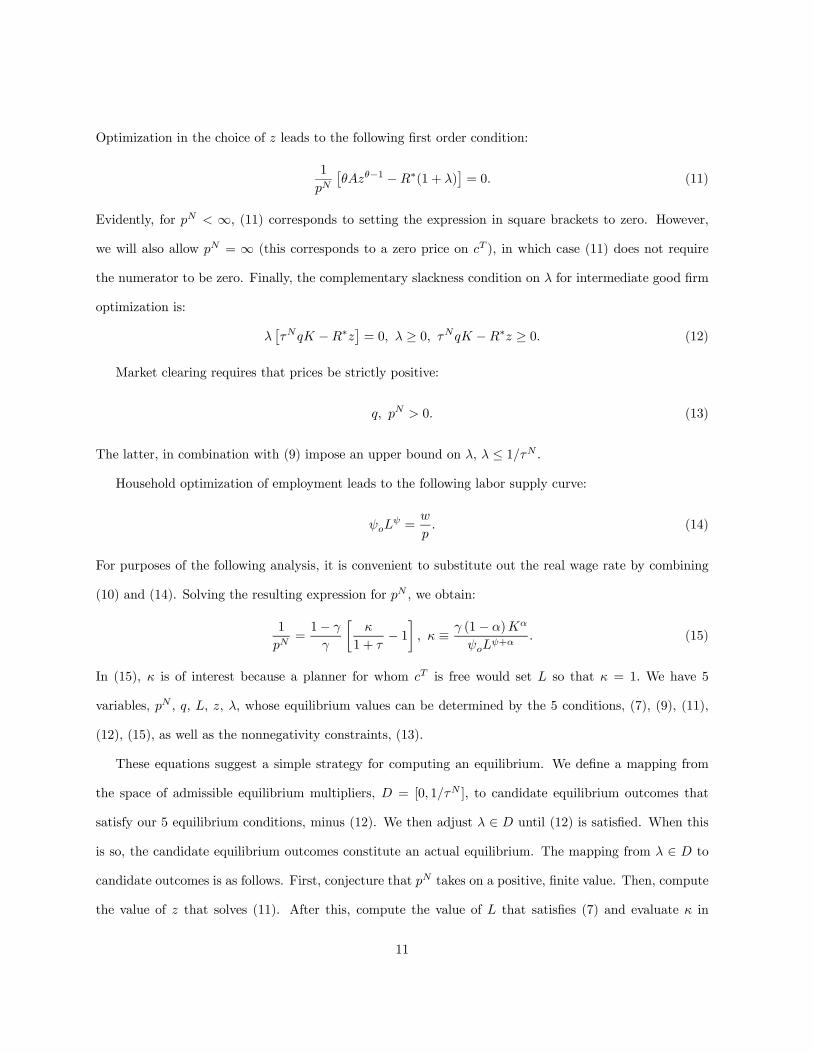
Optimization in the choice of z leads to the following first order condition:

1

pN£θAzθ−1 −R∗(1 + λ)

¤= 0. (11)

Evidently, for pN < ∞, (11) corresponds to setting the expression in square brackets to zero. However,

we will also allow pN = ∞ (this corresponds to a zero price on cT ), in which case (11) does not require

the numerator to be zero. Finally, the complementary slackness condition on λ for intermediate good firm

optimization is:

λ£τNqK −R∗z

¤= 0, λ ≥ 0, τNqK −R∗z ≥ 0. (12)

Market clearing requires that prices be strictly positive:

q, pN > 0. (13)

The latter, in combination with (9) impose an upper bound on λ, λ ≤ 1/τN .

Household optimization of employment leads to the following labor supply curve:

ψoLψ =

w

p. (14)

For purposes of the following analysis, it is convenient to substitute out the real wage rate by combining

(10) and (14). Solving the resulting expression for pN , we obtain:

1

pN=1− γ

γ

∙κ

1 + τ− 1¸, κ ≡ γ (1− α)Kα

ψoLψ+α

. (15)

In (15), κ is of interest because a planner for whom cT is free would set L so that κ = 1. We have 5

variables, pN , q, L, z, λ, whose equilibrium values can be determined by the 5 conditions, (7), (9), (11),

(12), (15), as well as the nonnegativity constraints, (13).

These equations suggest a simple strategy for computing an equilibrium. We define a mapping from

the space of admissible equilibrium multipliers, D = [0, 1/τN ], to candidate equilibrium outcomes that

satisfy our 5 equilibrium conditions, minus (12). We then adjust λ ∈ D until (12) is satisfied. When this

is so, the candidate equilibrium outcomes constitute an actual equilibrium. The mapping from λ ∈ D to

candidate outcomes is as follows. First, conjecture that pN takes on a positive, finite value. Then, compute

the value of z that solves (11). After this, compute the value of L that satisfies (7) and evaluate κ in

11

(15). If κ > (1 + τ), then use (15) to compute pN (note that the finiteness assumption on pN is verified).

In this case q can be computed from (9). Finally, compute τNqK − R∗z, so that (12) can be evaluated.

Now suppose κ ≤ (1 + τ). In this case, set pN =∞ (i.e., 1/pN = 0) and κ = 1 + τ . The latter expression

determines a value for L, which replaces the (smaller) value computed above. Solve for the smaller of the

two values of z which satisfy (7) with the given L. According to (9), q =∞ and therefore τNqK−R∗z =∞

also.

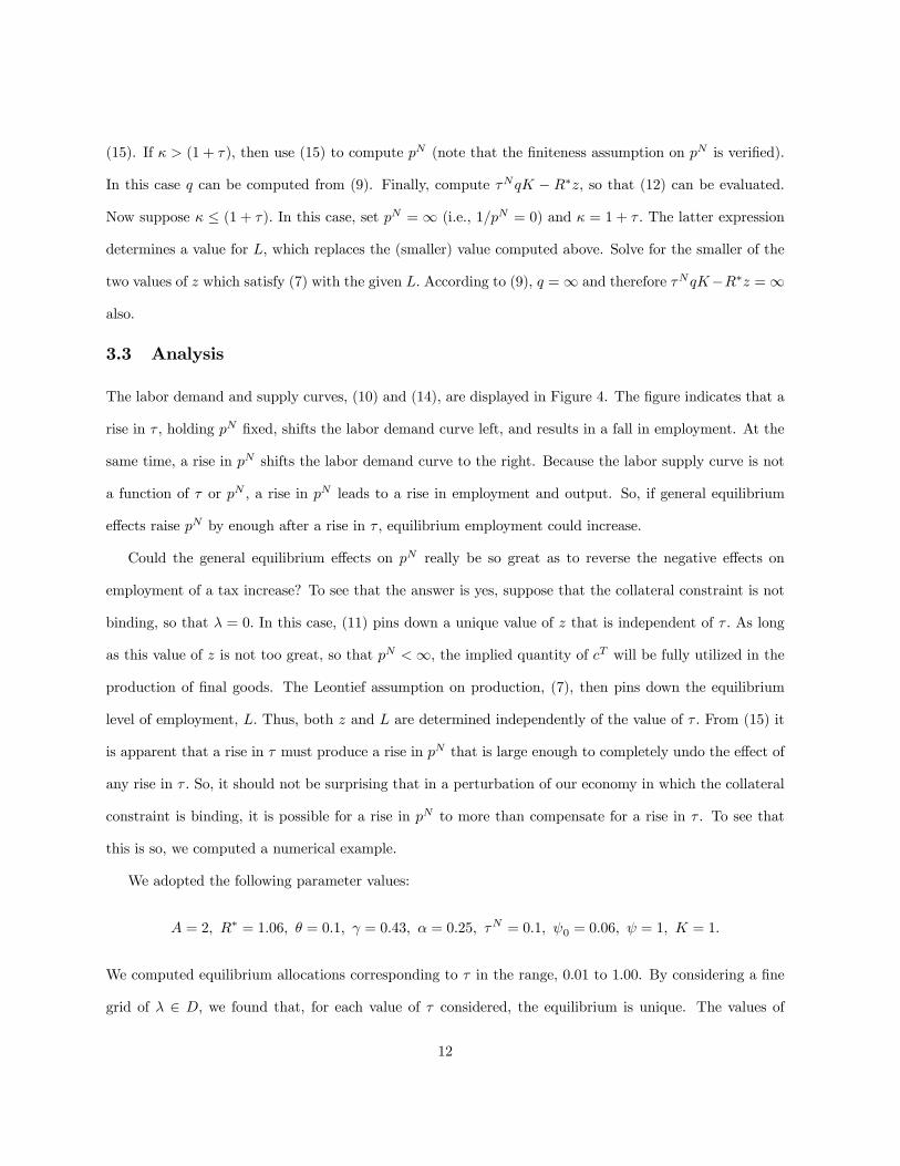
3.3 Analysis

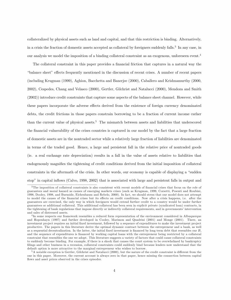
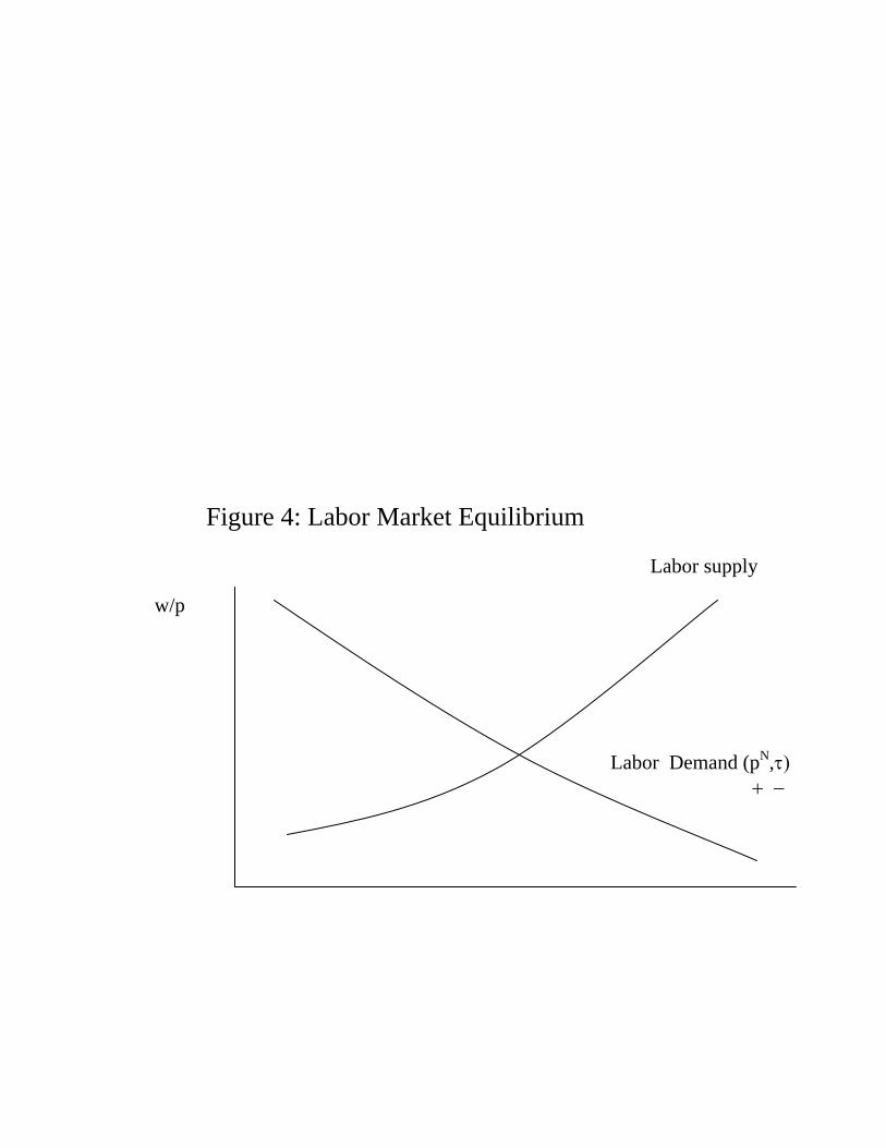
The labor demand and supply curves, (10) and (14), are displayed in Figure 4. The figure indicates that a

rise in τ , holding pN fixed, shifts the labor demand curve left, and results in a fall in employment. At the

same time, a rise in pN shifts the labor demand curve to the right. Because the labor supply curve is not

a function of τ or pN , a rise in pN leads to a rise in employment and output. So, if general equilibrium

effects raise pN by enough after a rise in τ , equilibrium employment could increase.

Could the general equilibrium effects on pN really be so great as to reverse the negative effects on

employment of a tax increase? To see that the answer is yes, suppose that the collateral constraint is not

binding, so that λ = 0. In this case, (11) pins down a unique value of z that is independent of τ . As long

as this value of z is not too great, so that pN <∞, the implied quantity of cT will be fully utilized in the

production of final goods. The Leontief assumption on production, (7), then pins down the equilibrium

level of employment, L. Thus, both z and L are determined independently of the value of τ . From (15) it

is apparent that a rise in τ must produce a rise in pN that is large enough to completely undo the effect of

any rise in τ . So, it should not be surprising that in a perturbation of our economy in which the collateral

constraint is binding, it is possible for a rise in pN to more than compensate for a rise in τ . To see that

this is so, we computed a numerical example.

We adopted the following parameter values:

A = 2, R∗ = 1.06, θ = 0.1, γ = 0.43, α = 0.25, τN = 0.1, ψ0 = 0.06, ψ = 1, K = 1.

We computed equilibrium allocations corresponding to τ in the range, 0.01 to 1.00. By considering a fine

grid of λ ∈ D, we found that, for each value of τ considered, the equilibrium is unique. The values of

12

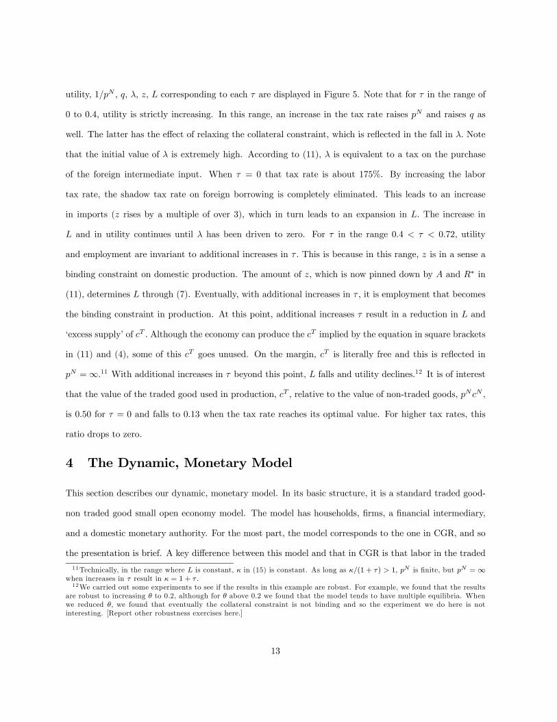
utility, 1/pN , q, λ, z, L corresponding to each τ are displayed in Figure 5. Note that for τ in the range of

0 to 0.4, utility is strictly increasing. In this range, an increase in the tax rate raises pN and raises q as

well. The latter has the effect of relaxing the collateral constraint, which is reflected in the fall in λ. Note

that the initial value of λ is extremely high. According to (11), λ is equivalent to a tax on the purchase

of the foreign intermediate input. When τ = 0 that tax rate is about 175%. By increasing the labor

tax rate, the shadow tax rate on foreign borrowing is completely eliminated. This leads to an increase

in imports (z rises by a multiple of over 3), which in turn leads to an expansion in L. The increase in

L and in utility continues until λ has been driven to zero. For τ in the range 0.4 < τ < 0.72, utility

and employment are invariant to additional increases in τ . This is because in this range, z is in a sense a

binding constraint on domestic production. The amount of z, which is now pinned down by A and R∗ in

(11), determines L through (7). Eventually, with additional increases in τ , it is employment that becomes

the binding constraint in production. At this point, additional increases τ result in a reduction in L and

‘excess supply’ of cT . Although the economy can produce the cT implied by the equation in square brackets

in (11) and (4), some of this cT goes unused. On the margin, cT is literally free and this is reflected in

pN =∞.11 With additional increases in τ beyond this point, L falls and utility declines.12 It is of interest

that the value of the traded good used in production, cT , relative to the value of non-traded goods, pNcN ,

is 0.50 for τ = 0 and falls to 0.13 when the tax rate reaches its optimal value. For higher tax rates, this

ratio drops to zero.

4 The Dynamic, Monetary Model

This section describes our dynamic, monetary model. In its basic structure, it is a standard traded good-

non traded good small open economy model. The model has households, firms, a financial intermediary,

and a domestic monetary authority. For the most part, the model corresponds to the one in CGR, and so

the presentation is brief. A key difference between this model and that in CGR is that labor in the traded

11Technically, in the range where L is constant, κ in (15) is constant. As long as κ/(1 + τ) > 1, pN is finite, but pN =∞when increases in τ result in κ = 1 + τ.12We carried out some experiments to see if the results in this example are robust. For example, we found that the results

are robust to increasing θ to 0.2, although for θ above 0.2 we found that the model tends to have multiple equilibria. Whenwe reduced θ, we found that eventually the collateral constraint is not binding and so the experiment we do here is notinteresting. [Report other robustness exercises here.]

13

good sector cannot be quickly adjusted in response to a shock.

4.1 Households

There is a representative household, which derives utility from consumption, ct, and leisure as follows:

∞Xt=0

βtu(ct, Lt), (3.1.1)

where Lt denotes labor time spent in the market and ct denotes consumption. We adopt the following

specification of utility:

u(c, L) =

hc− ψ0

1+ψL1+ψ

i1−σ1− σ

. (3.1.2)

The household begins the period with a stock of liquid assets, Mt. Of this, it allocates Qt to consumption

expenditures and the rest, Mt−Qt, is deposited with the financial intermediary. The cash constraint that

the household faces on its consumption expenditures is:

Ptct ≤WtLt +Qt, (17)

where Wt denotes the wage rate and Pt denotes the price level.

The household also faces a flow budget constraint governing the evolution of its assets:

Mt+1 = Rt(Mt −Qt +Xt) + PTt πt + [WtLt +Qt − Ptct] . (18)

Here, Rt denotes the gross domestic rate of interest, πt is profits which derive from household’s ownership

of firms, and Xt is a liquidity injection from the monetary authority. πt is measured in units of traded

goods, and PTt is the domestic currency price of traded goods. The term on the right of the equality reflects

the household’s sources of liquid assets at the beginning of period t+ 1 : interest earnings on deposits and

on the liquidity injection, profits and any cash that may be left unspent in the period t goods market.

The household maximizes (3.1.1) subject to (17)-(18), and the several timing constraints. Since the

model is deterministic after the first period, timing assumptions then do not matter. They do matter in the

first period, since the financial crisis is modeled as unanticipated in that period. So our timing assumptions

matter for the first periods. We assume that the employment decision is made at the very beginning of the

period, before any shock (e.g., the onset of the financial crisis) is realized. The household deposit decision

14

is made after the financial crisis occurs, but before the monetary authority’s response is realized. All other

household decisions are made after the monetary authority.

4.1.1 Firms

There are two types of representative, competitive, firms. The first produces the final consumption good,

c, purchased by households. Final goods production requires intermediate goods which are produced in

traded and non-traded good sectors by the second type of representative firm. We now discuss the decisions

facing these firms.

4.1.2 Final Good Firms

The production function of the final good firms is:

c = min©(1− γ) cT , γcN

ª, (19)

where cT and cN denote quantities of tradeable and non-tradeable intermediate inputs, respectively. As

noted above, the price of c is denoted by P, while PT and PN denote the money prices of the traded and

nontraded inputs, respectively. The firm takes these prices parametrically.

Zero profits and efficiency imply the following relation between prices:

p =1

1− γ+

pN

γ, p =

P

PT. (20)

The object, P, in the model corresponds to the model’s ‘consumer price index’, denominated in units of the

domestic currency. The object, p, is the consumer price index denominated in units of the traded good.

4.1.3 Intermediate Inputs

A single representative firm produces the traded and non-traded intermediate inputs. That firm manages

three types of debt, two of which are short-term. The firm borrows at the beginning of the period to finance

its wage bill and to purchase a foreign input, and repays these loans at the end of the period. In addition,

the firm holds the outstanding stock of external (net) indebtedness, Bt.

The firm’s optimization problem is:

max∞Xt=0

βtΛt+1πt, (21)

15

where

πt = pNt yNt + yTt − wN

t RtLNt − wT

t RtLTt −R∗zt − r∗Bt + (Bt+1 −Bt), (22)

denotes dividends, denominated in units of traded goods. Also, Bt is the stock of external debt at the

beginning of period t, denominated in units of the traded good; R∗ is the gross rate of interest (fixed in

units of the traded good) on loans for the purpose of purchasing zt; and r∗ is the net rate of interest (again,

fixed in terms of the traded good) on the outstanding stock of external debt. The price, Λt+1, is taken

parametrically by firms. In equilibrium, it is the multiplier on πt in the (Lagrangian representation of the)

household problem:13

Λt+1 = β

µuc,t+1P

Tt

Pt+1+Ωt+1P

Tt

¶= (23)

= βuc,t+1p

Tt

pt+1pTt+1

1

(1 + xt)

where

pTt =PTt

Mt.

qt =Qt

Mt.

Here,Mt is the aggregate stock of money at the beginning of period t, which is assumed to evolve according

to:

Mt+1

Mt= 1 + xt. (24)

Note that under our notational convention, all lower case prices except one, expresses that price in units of

the traded good. The exception, pTt , is the domestic currency price of traded goods, scaled by the beginning

of period stock of money. Alternatively, pTt is the inverse of a measure of real balances.

The firm production functions are:

yT =nθ [µ1V ]

ξ−1ξ + (1− θ) [µ2z]

ξ−1ξ

o ξξ−1

, (25)

V = A¡KT

¢ν ¡LT¢1−ν

,

yN =¡KN

¢α ¡LN¢1−α

,

13The intuition underlying (23) is straightforward. The object Λt+1 in (23), is the marginal utility of one unit of dividends,denominated in traded goods, transferred by the firm to the household at the end of period t. This corresponds to PT

t πt unitsof domestic currency. The households can use this currency in period t+1 to purchase PT

t πt/Pt+1 units of the consumptiongood. The value, in period t, of these units of consumption goods is βuc,t+1PT

t πt/Pt+1, or βuc,t+1PTt πt/(pt+1PT

t+1), whereuc,t is the marginal utility of consumption. This is the first expression in (23).

16

where ξ is the elasticity of substitution between value-added in the traded good sector, Vt, and the imported

intermediate good, zt. In the production functions, KT and KN denote capital in the traded and non-

traded good sectors, respectively. They are owned by the representative intermediate input firm. We keep

the stock of capital fixed throughout the analysis. It does not depreciate and there exists no technology

for making it bigger.

Total employment of the firm, Lt, is:

Lt = LTt + LNt .

We impose the following restriction on borrowing:

Bt+1

(1 + r∗)t→ 0, as t→∞. (26)

We suppose that international financial markets impose that this limit cannot be positive. That it cannot

be negative is an implication of firm optimality.

The firm’s problem at time t is to maximize (21) by choice of Bt+j+1, yNt+j , y

Tt+j , zt+j , L

Tt+j , L

Mt+j and

LNt+j , j = 0, 1, 2, ... and the indicated technology. In addition, the firm takes all prices and rates of return

as given and beyond its control. The firm also takes the initial stock of debt, Bt, as given. This completes

the description of the firm problem in the pre-crisis version of the model, when collateral constraints are

ignored.

The crisis brings on the imposition of the following collateral constraint:

τNqNt KN + τT qTt KT ≥ R∗zt + (1 + r∗)Bt + ζRt

¡WT

t LTt +WN

t LNt¢

(27)

Here, qi, i = N,T denote the value (in units of the traded good) of a unit of capital in the nontraded and

traded good sectors, respectively. Also, τ i denotes the fraction of these stocks accepted as collateral by

international creditors. The left side of (27) is the total value of collateral, and the right side is the payout

value of the firm’s external debt; ζ indicates the fraction of the wage bill that enters into the liabilities side

of the collateral constraint, and represents the share of domestic loans that are collateralized and would

compete with foreign creditors’ claims on the firm’s assets. Before the crisis, firms ignore (27), and assign

17

a zero probability that it will be implemented. With the coming of the crisis, firms believe that (27) must

be satisfied in every period henceforth, and do not entertain the possibility that it will be removed.

We obtain qNt and qTt by differentiating the Lagrangian representation of the firm optimization problem

with respect to KN and KT , respectively. The equilibrium value of the asset prices, qit, i = N,T, is the

amount that a potential firm would be willing to pay in period t, in units of the traded good, to acquire

a unit of capital and start production in period t. We let λt ≥ 0 denote the multiplier on the collateral

constraint (= 0 in the pre-crisis period) in firm problem. Then, qit solves

qit =VMP i

k,t + β Λt+2Λt+1qit+1

1− λtτ i, i = N,T. (28)

Here, VMP ik,t denotes the period t value (in terms of traded goods) marginal product of capital in sector

i.

When λt ≡ 0, (28) is just the standard asset pricing equation. It is the present discounted value of the

value of the marginal physical product of capital. When the collateral constraint is binding, so that λt is

positive, then qit is greater than this. This reflects that in this case capital is not only useful in production,

but also for relieving the collateral constraint. In our model capital is never actually traded since all firms

are identical. However, if there were trade, then the price of capital would be qit. If a firm were to default

on its credit obligations, the notion is that foreign creditors could compel the sale of its physical assets in

a domestic market for capital. The price, qit, is how much traded goods a domestic resident is willing to

pay for a unit of capital. Foreign creditors would receive those goods in the event of a default. We assume

that with these consequences for default, default never occurs in equilibrium.

To understand the impact of a binding collateral constraint on firm decisions, it is useful to consider

the Euler equations of the firm. Differentiating Lagrangian representation of the firm problem with respect

to Bt+1:

1 = βΛt+2Λt+1

(1 + r∗)(1 + λt+1), t = 0, 1, 2, ... . (29)

Following standard practice in the small open economy literature, we assume β(1 + r∗) = 1, so that14

Λt+1 = Λt+2(1 + λt+1), t = 0, 1, 2, ... . (30)

14See, for example, Obstfeld and Rogoff (1997).

18

A high value for λ, which occurs when the collateral constraint is binding, raises the effective rate of interest

on debt. The interpretation is that when λ is large, then the debt has an additional cost, beyond the direct

interest cost. This cost reflects that when the firm raises Bt+1 in period t, it not only incurs an additional

interest charge in period t+ 1, but it is also further tightens its collateral constraint in that period. This

has a cost because, via the collateral constraint, the extra debt inhibits the firm’s ability to acquire working

capital in period t + 1. Thus, when λ is high, there is an additional incentive for firms to reduce π and

‘save’ by paying down the external debt. Although the firm’s actual interest rate on external debt taken

on in period t is 1 + r∗, it’s ‘effective’ interest rate is (1 + r∗) (1 + λt+1) .

4.2 Financial Intermediary and Monetary Authority

The financial intermediary takes domestic currency deposits, Dt = Mt − Qt, from the household at the

beginning of period t. In addition, it receives the liquidity transfer, Xt = xtMt, from the monetary

authority.15 It then lends all its domestic funds to firms who use it to finance their employment working

capital requirements, WL. Clearing in the money market requires Mt −Qt +Xt =WtLt, or, after scaling

by the aggregate money stock,

dt + xt = pTt£wNt L

Nt + wT

t LTt

¤, (31)

where dt = Dt/Mt.

The monetary authority in our model simply injects funds into the financial intermediary. Its period t

decision is taken after the household has selected a value forQt, and before all other variables in the economy

are determined. This is the standard assumption in the limited participation literature. It is interpreted

as reflecting a sluggishness in the response of household portfolio decisions to changes in market variables.

With this assumption, a value of xt that deviates from what households expected at the time Qt was set

produces an immediate reaction by firms and the financial intermediary but not, in the first instance, by

households. The name, ‘limited participation’, derives from this feature, namely that not all agents react

immediately to (or, ‘participate in’) a monetary shock. As a result of this timing assumption, many models

15 In practice, injections of liquidity do not occur in the form of lump sum transfers, as they do here. It is easy to showthat our formulation is equivalent to an alternative, in which the injection occurs as a result of an open market purchaseof government bonds which are owned by the household, but held by the financial intermediary. We do not adopt thisinterpretation in our formal model in order to conserve on notation.

19

exhibit the following behavior in equilibrium. An unexpectedly high value of xt swells the supply of funds

in the financial sector. To get firms to absorb the increase in funds, a fall in the equilibrium rate of interest

is required. When that fall does occur, they borrow the increased funds and use them to hire more labor

and produce more output.

We abstract from all other aspects of government finance. The only policy variable of the government

is xt.

4.3 Equilibrium

We consider a perfect foresight, sequence-of-market equilibrium concept. In particular, it is a sequence of

prices and quantities having the properties: (i) for each date, the quantities solve the household and firm

problems, given the prices, and (ii) the labor, goods and domestic money markets clear.

Clearing in the money market requires that (31) hold and that actual money balances,Mt, equal desired

money balances, Mt. Combining this with the household’s cash constraint, (17), we obtain the equilibrium

cash constraint:

pTt ptct = 1 + xt. (32)

According to this, the total, end of period stock of money must equal the value of final output, ct. Market

clearing in the traded good sector requires:

yTt −R∗zt − r∗Bt − cTt = − (Bt+1 −Bt) . (33)

The left side of this expression is the current account of the balance of payments, i.e., total production

of traded goods, net of foreign interest payments, net of domestic consumption. The right side of (33) is

the change in net foreign assets. Equation (33) reflects our assumption that external borrowing to finance

the intermediate good, zt, is fully paid back at the end of the period. That is, this borrowing resembles

short-term trade credit. Note, however, that this is not a binding constraint on the firm, since our setup

permits the firm to finance these repayments using long term debt. Market clearing in the nontraded good

sector requires:

yNt = cNt . (34)

20

Our procedure for computing the equilibrium of the model is a generalization on the multiplier-based

method used in section 3. It corresponds a variation on the procedure applied in CGR and the details are

available from the authors on request.

5 Quantitative Analysis

In this section we begin with a discussion of the parameterization of the model. We then report the results

for optimal monetary policy.

5.1 Parameter Values and Steady State

The parameter values are displayed in Table 3. These were chosen to so that the model’s steady state in

the absence of collateral constraints roughly matches features of Korean and Thai data during the first

semester of 1997. The share of tradables in total production for Korea, assuming that tradables correspond

to the non-service sectors, was approximately one third before the crisis. Combining this assumption

with estimates of labor shares from A. Young (1995), we estimate shares of capital for the tradable and

nontradable sector in Korea to be respectively 0.48 and 0.21. Based on figures for Argentina, Uribe (1995)

and Rebelo and Vegh (1995) estimate the same shares to be 0.52 and 0.37. We take an intermediate

point between these estimates by specifying ν = 0.50 and α = 0.36. Reinhart and Vegh (1995) estimate

the elasticity of intertemporal substitution in consumption for Argentina to be equal to 0.2. We adopt a

somewhat higher elasticity by setting σ = 2.We take the foreign interest rate to be equal to 6 percent and

we assume a rate of money growth of 6 percent to obtain a nominal domestic interest rate of 12.3 percent,

roughly in line with the experience of Korea and Thailand in the years before the crises. We set ψ = 3,

implying a labor supply elasticity of 1/3. This is low by comparison to that used in standard business cycle

models. Our choice of a low labor supply elasticity is conservative. We presume that a higher labor supply

elasticity would have simply resulted in a smaller recession.

The parameters µ1 and µ2, in the production function were chosen to reproduce the ratio of imported

intermediate inputs in manufacturing to manufacturing value-added in Korea for the year 1995. In that

year the ratio is 0.4, in other words z/V = 0.4.

As mentioned above, the share of tradable goods in production is roughly one third, so we calibrate

21

the remaining parameters of the model to produce a ratio of consumption of nontradables to tradables of

approximately 2. In addition, we chose τ and the stock of debt in the initial steady state equilibrium so

that the initial and final debt to output ratio correspond roughly to the experience of Korea and Thailand.

Korea’s (Thailand’s) external debt started at 33% of GDP by end-1997 (60.3%) and was around 26.8% of

GDP (51% of GDP) and the end of the year 2000. The interest rate in the initial steady state is set to

11 percent, in annual terms. This is very close to the pre-crisis interest rates in Korea and Thailand. The

pre-crisis steady state of the model is reported in Table 4.

5.2 Optimal Monetary Policy

We now consider the dynamic effects of the imposition of the collateral constraint—our reduced form,

underlying source of the financial crisis—and the implementation of the optimal monetary policy in this

context. The timing of the experiment can be seen in Figure 6. Up until period 0, the economy is in

a nonstochastic steady state in which the collateral constraint is not binding. At the start of period 0,

the household makes its employment decision in the traded sector. After this, the collateral constraint on

borrowing is unexpectedly imposed. This constraint is binding. Then, the household makes its deposit

decision. In making its deposit decision the household assumes money growth will continue at its previous

constant rate. After this, the monetary action occurs. Finally, all activity occurs. The remainder of all

time unfolds in a non-stochastic way. The collateral constraint remains in force for ever after.

The results are reported in Figure 7. A period in the model is taken to be 6 months. As a benchmark,

we include actual (semi-annual) data for Korea. Note the sharp rise in the current account. Also, the

drop in GDP, relative to its pre-crisis trend, is nearly 15 percent. The drop in employment is less, though

it takes longer to recover. Interestingly, this represents a substantial drop in labor productivity. The

drop in consumption is a little larger and more persistent than the drop in output. Share prices fall and

then recover. The interest rate rises sharply (as noted in Figure 1), and then falls substantially below its

pre-crisis level. The exchange rate initially depreciates by about 50 percent, although the depreciation

is ultimately smaller. Finally, inflation jumps from about 5 percent initially to about 12 percent, before

stabilizing at a lower level.

22

Now consider the response of the model under the optimal monetary policy. Note that the current

account in the model increases, though not as much as in the Korean data. We suspect that the absence

of investment in our model is part of the reason for this. With domestic investment there is an additional

margin that can be used to cut back domestic absorption and increase the current account. We expect that

in a version of our model with investment, agents would exploit this margin given the very high value of the

multiplier on the collateral constraint. The drop in domestic output is of a similar order of magnitude as

the drop in output in Korea, though somewhat smaller. In the case of employment, the model substantially

overstates the drop. This is an interesting miss. In effect, the model cannot explain the substantial drop

in labor productivity observed in the wake of the Korean financial crisis. The model matches the behavior

of asset prices and the nominal exchange rate quite well. However, the model substantially overstates the

nominal interest rate and the rate of inflation in the wake of the Korean crisis.

Overall, we believe that the model captures reasonably well the behavior of the Korean data during

the currency crisis. Figure 8 helps to assess the optimal monetary policy by comparing it with a particular

benchmark. In the benchmark, money growth is held fixed at its pre-shock level. Note that relative to

this benchmark, the optimal monetary policy stimulates aggregate output, consumption, employment and

imports. It does so by raising the nominal interest rate substantially.

The economic intuition underlying these results can be found in contemplating the collateral constraint.

The rise of the interest rate in period 0 slows the exchange rate depreciation and this contributes to a smaller

reduction in asset prices. This relative improvement on the asset side of the collateral constraint allows for

a smaller drop in imports of intermediate inputs, and a smaller reduction in real GDP, employment and

consumption. Once the initial increase in interest rates and exchange rate depreciation set in motion the

external adjustment process, labor is reallocated to the traded sector. From that moment onwards, the

optimal monetary policy consists of reducing interest rate to values very close to the arrival steady state

level of 2%. It is worth noting that during this transition period, and in consonance with the evidence on

the crises countries, interest rate cuts are associated with nominal (and real) exchange rate depreciations

(Mussa, 2000).

23

6 Conclusions

In this paper we studied the optimal monetary policy response to a financial crisis of the kind experienced by

the Asian economies in 1997-98. These crises, as many other emerging market crises, were characterized by

a sudden reversals in capital inflows. Using a fairly general open economy model with collateral constraints,

we found that the optimal monetary response to such crises involves and initial increase in interest rates,

followed by a relatively sharp and rapid reduction in rates in the aftermath of the crisis. The optimal

monetary policy does not avoid the recessionary effects of the sudden stop, but it attenuates the fall in

asset prices, output and employment, and allows for better consumption smoothing opportunities.

The collateral constraint captures the balance sheet constraints discussed by policymakers as constraints

on credit conditions and on the conduct of monetary policy. The optimal monetary policy in such crises,

and its implications for other macro variables as predicted by the model, are similar to the evolution of

actual variables in the cases of Korea and Thailand.

24

References

[1] Aghion, Philippe, Philippe Bacchetta, Abhijit Banerjee, 2000, “Currency Crises and Monetary Policy

in an Economy with Credit Constraints”, mimeo.

[2] Asea, Patrick and B. Blomberg, 1998, “Lending Cycles”, Journal of Econometrics, 83: 89-128.

[3] Auernheimer, Leonardo and Roberto Garcia-Saltos, 1999, “International Debt and the Price of Do-

mestic Assets”, mimeo.

[4] Berger, Allen and Gregory Udell, 1990, “Collateral, Loan Quality and Bank Risk”, Journal of Mone-

tary Economics, 25:21-42.

[5] Black, Jane, David de Meza and David Jeffreys, 1996, “House Prices, the Supply of Collateral and the

Enterprise Economy”, The Economic Journal, 106: 60-75.

[6] Boorman, Jack, T. Lane, M.Schulze-Gattas, A. Bulir, A. Ghosh, J. Hamann, A. Mourmouras,

S.Phillips, 2000, “Managing Financial Crises: The Experience in East Asia”, forthcoming, Carnegie

-Rochester Conference Series on Public Policy.

[7] Burnside, Craig, Martin Eichenbaum and Sergio Rebelo, 1999, “Hedging and Financial Fragility in

Fixed Exchange Rate Systems”, NBER Working Paper No. 7143.

[8] Caballero, Ricardo and Arvind Krishnamurty, 1999, “Emerging Markets Crises: An Asset Markets

Perspective”, mimeo.

[9] Calvo, Guillermo, 1998, “Capital Flows and Capital Market Crises”, mimeo, University of Maryland.

[10] Cespedes, Luis, Roberto Chang and Andres Velasco, 2000, “Balance Sheets and Exchange Rate Pol-

icy”, mimeo.

[11] Chadha, Bankim and David Folkerts-Landau, 1999,“The Evolving Role of Banks in International

Capital Flows”, in Feldstein ed., International Capital Flows, The University of Chicago Press.

25

[12] Christiano, Lawrence J. and Martin Eichenbaum, “Liquidity Effects and The Monetary Transmission

Mechanism”, American Economic Review, 82: 346-53.

[13] Christiano, Lawrence J. and Martin Eichenbaum, “Liquidity Effects, Monetary Policy and the Business

Cycle”, Journal of Money, Credit and Banking, 27: 1113-1136.

[14] Christiano, Lawrence J., Christopher Gust and Jorge Roldos, 2004, ”Monetary Policy in a Financial

Crisis”, Journal of Economic Theory, Volume 119, Issue 1, Pages 1-245, November.

[15] Corsetti, G., C. Pesenti and N. Roubini, 1998, ”What Caused the Asian Currency and Financial

Crisis? Part I: A Macroeconomic Overview”, NBER Working Paper No. 6833.

[16] Dooley, Michael, 2000, “A Model of Crises in Emerging Markets”, The Economic Journal, 110: 256-

272.

[17] Eaton, Jonathan, Gersowitz and J. Stiglitz, 1986, “The Pure Theory of Country Risk”, European

Economic Review;

[18] Edison, Hali, Pongsak Luangaram and Marcus Miller, 2000, “Asset Bubbles, Leverage and “Lifeboats”:

Elements of the East Asian Crisis”, The Economic Journal, 110: 245-255.

[19] Fuerst, Timothy, 1992, “Liquidity, Loanable Funds, and Real Activity”, Journal of Monetary Eco-

nomics, 29: 3-24.

[20] Gelos, Gaston and Alejandro Werner, 1999, “Financial Liberalization, Credit Constraints and Collat-

eral: Investment in the Mexican Manufacturing Sector”, IMF Working Paper No.99/25.

[21] Gertler, Mark, Simon Gilchrist and Fabio Natalucci, 2000, “External Constraints and the Financial

Accelerator”, mimeo.

[22] Kiyotaki, Nobuhiro, and John Moore, 1997, “Credit Cycles” Journal of Political Economy, 105: 211-

248.

26

[23] Krugman, Paul, 1999, “Balance Sheets, the Transfer Problem, and Financial Crises”, in P.Isard, A.

Razin and A.Rose, eds., International Finance and Financial Crises: Essays in Honor of Robert P.

Flood, Jr., Kluwer Academic Publishers.

[24] Krugman, Paul, 1999, The Return of Depression Economics, WW Norton &Company, New York.

[25] Lucas, Robert E., 1990, “Liquidity and Interest Rates”, Journal of Economic Theory, 50:273-264.

[26] Mendoza, Enrique, 2001, “The Benefits of Dollarization when Stabilization Policy Lacks Credibility

and Financial Markets are Imperfect”, Journal of Money, Credit and Banking.

[27] Mussa, Michael, 2000, “Using Monetary Policy to Resist Exchange Rate Depreciation”, mimeo, IMF.

[28] Obstfeld, Maurice, and Kenneth Rogoff, 1997, Foundations of International Macroeconomics, MIT

Press.

[29] Rebelo, Sergio and Carlos Vegh, 1995, “Real Effects of Exchange-rate-based Stabilization: An Analysis

of Competitng Theories”, NBER Macroeconomics Annual, 125-187.

[30] Uribe, Martin, 1997, “Exchange-rate-based Inflation Stabilization: The Initial Real Effects of Credible

Plans”, Journal of Monetary Economics, 39: 197-221.

[31] Young, Alwyn, 1995, “The Tyranny of Numbers: Confronting the Statistical Realities of the East

Asian Growth Experience”, Quarterly Journal of Economics, 110(3): 641-680.

27

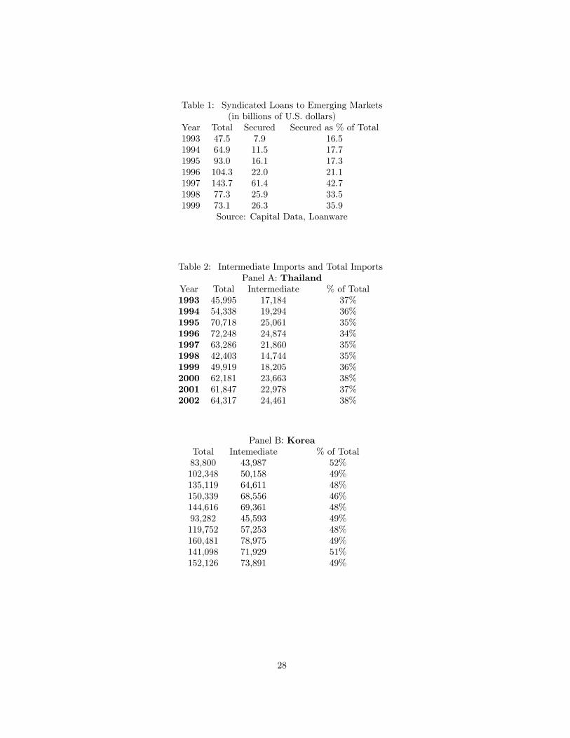
Table 1: Syndicated Loans to Emerging Markets(in billions of U.S. dollars)

Year Total Secured Secured as % of Total1993 47.5 7.9 16.51994 64.9 11.5 17.71995 93.0 16.1 17.31996 104.3 22.0 21.11997 143.7 61.4 42.71998 77.3 25.9 33.51999 73.1 26.3 35.9

Source: Capital Data, Loanware

Table 2: Intermediate Imports and Total ImportsPanel A: Thailand

Year Total Intermediate % of Total1993 45,995 17,184 37%1994 54,338 19,294 36%1995 70,718 25,061 35%1996 72,248 24,874 34%1997 63,286 21,860 35%1998 42,403 14,744 35%1999 49,919 18,205 36%2000 62,181 23,663 38%2001 61,847 22,978 37%2002 64,317 24,461 38%

Panel B: KoreaTotal Intemediate % of Total83,800 43,987 52%102,348 50,158 49%135,119 64,611 48%150,339 68,556 46%144,616 69,361 48%93,282 45,593 49%119,752 57,253 48%160,481 78,975 49%141,098 71,929 51%152,126 73,891 49%

28

Panel C: MalaysiaYear Total Intermediate % of Total199319941995 77,601 50,447 65%1996 78,426 52,201 67%1997 79,036 51,922 66%1998 58,293 40,901 70%1999 65,389 48,321 74%2000 81,963 61,233 75%2001 73,856 53,271 72%2002 79,881 56,939 71%

Panel D: IndonesiaTotal Intermediate % of Total28,376 20,035 71%32,222 23,146 72%40,921 29,610 72%44,240 30,470 69%46,223 30,230 65%31,942 19,612 61%30,600 18,475 60%40,367 26,073 65%34,669 23,879 69%

24,118

Panel E: PhilippinesYear Total Intermediate % of Total1993 17,597 7,855 45%1994 21,333 9,559 45%1995 26,538 12,174 46%1996 32,427 14,015 43%1997 35,933 14,663 41%1998 29,660 11,586 39%1999 30,726 12,596 41%2000 34,491 16,747 49%2001 33,058 15,121 46%2002 35,427 14,791 42%

Source: CEIC

29

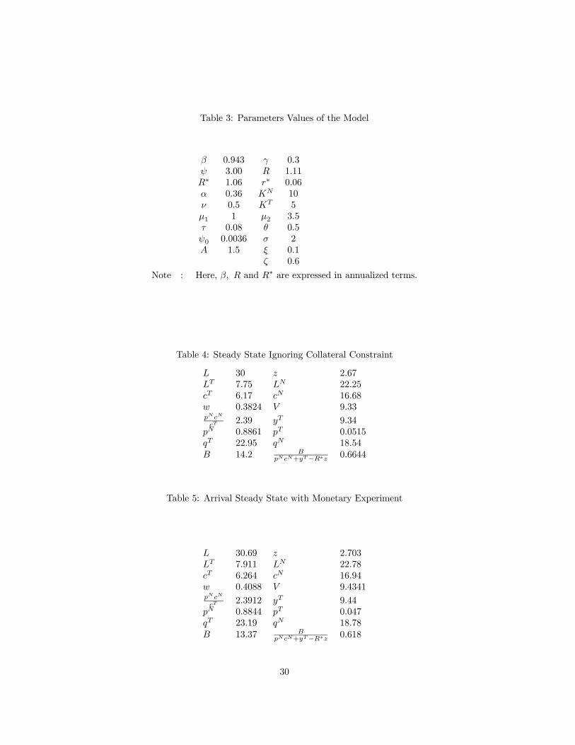
Table 3: Parameters Values of the Model

β 0.943 γ 0.3ψ 3.00 R 1.11R∗ 1.06 r∗ 0.06α 0.36 KN 10ν 0.5 KT 5µ1 1 µ2 3.5τ 0.08 θ 0.5ψ0 0.0036 σ 2A 1.5 ξ 0.1

ζ 0.6

Note : Here, β, R and R∗ are expressed in annualized terms.

Table 4: Steady State Ignoring Collateral Constraint

L 30 z 2.67LT 7.75 LN 22.25cT 6.17 cN 16.68w 0.3824 V 9.33pNcN

cT 2.39 yT 9.34pN 0.8861 pT 0.0515qT 22.95 qN 18.54B 14.2 B

pNcN+yT−R∗z 0.6644

Table 5: Arrival Steady State with Monetary Experiment

L 30.69 z 2.703LT 7.911 LN 22.78cT 6.264 cN 16.94w 0.4088 V 9.4341pNcN

cT 2.3912 yT 9.44pN 0.8844 pT 0.047qT 23.19 qN 18.78B 13.37 B

pNcN+yT−R∗z 0.618

30

SHORT-TERM INTEREST RATES 1/

0

5

10

15

20

25

30

35

Jan-97 Jan-98 Jan-99 Jan-000

5

10

15

20

25

30

35

ThailandKoreaMalaysiaPhilippines

Figure 1

Intermediate Goods Import vs. GDP(Index 1995 = 100)

Sources: CEIC; and WEO.

Indonesia

GDP

0

20

40

60

80

100

120

140

1993 1995 1997 1999 20010

20

40

60

80

100

120

140

Intermediate

Korea

GDP

0

20

40

60

80

100

120

140

1993 1995 1997 1999 20010

20

40

60

80

100

120

140

Malaysia

GDP

0

20

40

60

80

100

120

140

1993 1995 1997 1999 20010

20

40

60

80

100

120

140

Intermediate Philippines

GDP

0

20

40

60

80

100

120

140

1993 1995 1997 1999 20010

20

40

60

80

100

120

140

Intermediate

Thailand

GDP

0

20

40

60

80

100

120

140

1993 1995 1997 1999 20010

20

40

60

80

100

120

140

Intermediate

Figure 2

EXCHANGE RATES (national currency/US$)

70

90

110

130

150

170

190

210

230

Jan-97 Jan-98 Jan-99 Jan-0070

90

110

130

150

170

190

210

230

ThailandPhilippinesMalaysiaKorea

Figure 3

Labor Demand (pN,τ) + −

Labor supply

w/p

Figure 4: Labor Market Equilibrium

0 0.5 1

0.64

0.65

0.66

0.67utility

τ0 0.5 1

0

0.2

0.4

0.6

0.8

1

1/pN

τ

0 0.5 1

0.96

0.98

1

1.02

1.04

1.06

L

τ

0 0.5 10

10

20

30

40

50q

τ

0 0.5 1

0

0.5

1

1.5

λ

τ

Figure 5: Equilibrium Associated With Various Tax Rates

0 0.5 11

1.5

2

2.5

3

3.5z

τ

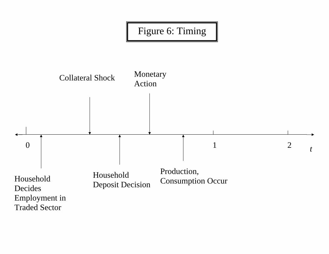
Figure 6: Timing

Collateral Shock

Household Deposit Decision

Monetary Action

Production, Consumption Occur

0 1 2 t

Household Decides Employment in Traded Sector

Figure 7: Optimal and Constant Money Growth

0

0.1

0.2current account

SimulationActual Korean Data

-15

-10

-5

0

5real GDP

-20

-10

0

10Employment

-20

-10

0

10Consumption

-10

0

10Imports

-20

-10

0

10Asset Prices

0

20

40Nominal Interest Rate

1

1.2

1.4

1.6Nominal Exchange Rate (Price of Traded)

-200

204060

Inflation

Figure 8: Optimal and Constant Money Growth

0

0.02

0.04current account

Optimal Money GrowthConstant Money Growth

-15

-10

-5

0

5real GDP

-20

-10

0

10Employment

-20

-10

0

10Consumption

-10

0

10Imports

-20

-10

0

10Asset Prices

0

20

40Nominal Interest Rate

1

1.2

1.4

1.6Nominal Exchange Rate (Price of Traded)

-200

204060

Inflation