Notes on Digital Filtering

Rick Aster and Brian Borchers

October 28, 2002

Digital Filtering

We next turn to the (very broad) topic of how to manipulate a sampled signal to alterthe amplitude and/or phase of different frequency components of the signal. There is anincredible amount of literature on this subject, and we will only be able to scratch thesurface here. There are many reasons for wanting to filter a signal including:

1. Noise rejection/Signal enhancement

2. Remove an instrument response from the signal

3. Differentiate or integrate

4. Change the sampling rate

5. Artistic effects in audio and video.

Some particular types of filters that we will look at include low pass, high pass,and band pass filters which cut off portions of the frequency spectrum while allowingother frequencies to pass through the filter. In implementing these filters we will wantto achieve the desired frequency response while otherwise distorting the signal as littleas possible.

We will concentrate our analysis on filters which are themselves linear time invariantsystems. This will enable us to apply all of the techniques that we have previouslydeveloped for LTI systems to analyze the performance of the filter. However, it is alsopossible to construct more complicated nonlinear filters which are not LTI systems.

In analyzing filters we will again encounter the concept of stability. A linear filteris stable if the corresponding LTI is stable. If we try to use an unstable filter, we’re likelyto find that small amounts of noise in the input build up in the output to intolerablelevels. Unstable filters are practically impossible to use.

In some cases a filter is designed to process the signal in real time with little or nodelay, while in other cases we must receive the entire signal before we can begin processingit. There is generally a preference for linear filters which are causal, since these filters canbe implemented in real time. If an acausal filter needs to look ahead only a few samples,

1

then we can implement the filter in real time by simply inserting a buffer before the filterand allowing the filter to delay its output by a few samples.

In practice, much of the human effort that goes into designing and implementingdigital filters is about tradeoffs between the desired frequency and phase response of thefilter and difficulty and cost of the implementation of the filter.

Filtering by Direct Manipulation of the FFT

One very simple approach to filtering a sampled signal is to compute its FFT and thenmanipulate the individual components of the FFT to achieve a desired frequency or phaseresponse. This approach gives us complete freedom to control the frequency and phaseresponse of the filter.

There are two significant costs associated with implementing a filter in this fashion.The first problem is that computing the FFT of a signal can (depending on the samplingrate and time duration of the signal) be very computationally intensive. For very longsignals, computing the FFT of the entire signal may not even be practical. The secondissue is that since we must have the entire signal in hand before we can begin filtering,we cannot use this method for real time filtering.

For example, consider a 20 second long recording of some guitar music. (The audioclip and MATLAB codes for this example will be made available on the class web site.)The audio is digitized according to the consumer audio CD standard at a sample rate of44.1 Khz, with 16 bits per sample. For this example, we’ve combined the left and rightchannels into one mono channel. Thus the 20 seconds of audio requires 20× 44100× 16bits, or 1.76 megabytes of storage. We’ll store the samples in MATLAB as 8 byte doubleprecision numbers, which expands the storage requirements by a factor of four to about8 megabytes. This is fairly large, but still well within the memory size limits of ourcomputers.

At the sampling rate of 44.1 Khz, the Nyquist frequency is 22.05 Khz. Is a practicalmatter, most of us can’t hear (and the speakers in our classroom can’t reproduce) muchabove about 15 Khz. Before sampling, this signal was passed through an analog anti-aliasing filter that eliminated all frequencies above 22.05 Khz. Thus the sampling ratehas been chosen to effectively reproduce all of the frequencies in the original music whileavoiding aliasing problems.

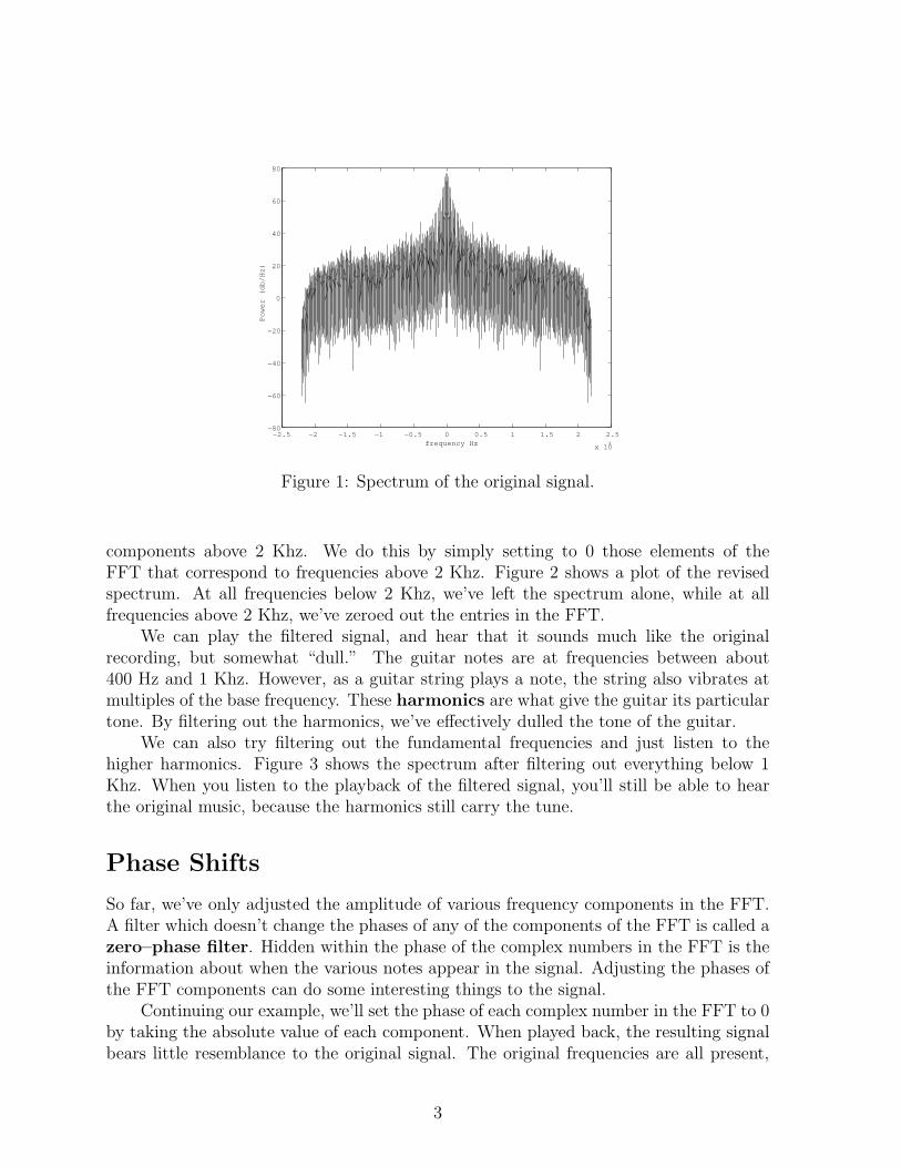
We read the signal into MATLAB and compute its FFT. Since there are 882,000real values in the original signal, the FFT also has 882,000 complex components. Sincethere are 882,000 frequency components over a frequency range of 0 to 44,100 Hz, eachcomponent of the FFT represents a frequency range of 0.05 Hz. Figure 1 shows a plot ofthe absolute values of the FFT versus frequency. The vertical aix represents power. Wehave used a dB scale. The horizontal access represents frequency in Hz. For convenience,we have used the MATLAB command fftshift to rearrange the entries in the FFT sothat 0 Hz is at the center of the spectrum.

Now, suppose that we want to low pass filter the signal, eliminating all frequency

2

−2.5 −2 −1.5 −1 −0.5 0 0.5 1 1.5 2 2.5

x 104

−80

−60

−40

−20

0

20

40

60

80

frequency Hz

Po

we

r (d

b/H

z)

Figure 1: Spectrum of the original signal.

components above 2 Khz. We do this by simply setting to 0 those elements of theFFT that correspond to frequencies above 2 Khz. Figure 2 shows a plot of the revisedspectrum. At all frequencies below 2 Khz, we’ve left the spectrum alone, while at allfrequencies above 2 Khz, we’ve zeroed out the entries in the FFT.

We can play the filtered signal, and hear that it sounds much like the originalrecording, but somewhat “dull.” The guitar notes are at frequencies between about400 Hz and 1 Khz. However, as a guitar string plays a note, the string also vibrates atmultiples of the base frequency. These harmonics are what give the guitar its particulartone. By filtering out the harmonics, we’ve effectively dulled the tone of the guitar.

We can also try filtering out the fundamental frequencies and just listen to thehigher harmonics. Figure 3 shows the spectrum after filtering out everything below 1Khz. When you listen to the playback of the filtered signal, you’ll still be able to hearthe original music, because the harmonics still carry the tune.

Phase Shifts

So far, we’ve only adjusted the amplitude of various frequency components in the FFT.A filter which doesn’t change the phases of any of the components of the FFT is called azero–phase filter. Hidden within the phase of the complex numbers in the FFT is theinformation about when the various notes appear in the signal. Adjusting the phases ofthe FFT components can do some interesting things to the signal.

Continuing our example, we’ll set the phase of each complex number in the FFT to 0by taking the absolute value of each component. When played back, the resulting signalbears little resemblance to the original signal. The original frequencies are all present,

3

−2.5 −2 −1.5 −1 −0.5 0 0.5 1 1.5 2 2.5

x 104

−100

−50

0

50

100

150

200

frequency Hz

Po

we

r (d

b/H

z)

Figure 2: Spectrum after low pass filtering.

−2.5 −2 −1.5 −1 −0.5 0 0.5 1 1.5 2 2.5

x 104

−80

−60

−40

−20

0

20

40

60

frequency Hz

Po

we

r (d

b/H

z)

Figure 3: Spectrum after high pass filtering.

4

but the order of the notes has disappeared completely.In general, filtering that effects phase can cause distortion in the signal that will make

it virtually unrecognizable. However, there is one important type of phase adjustmentthat can be tolerated and is fact useful in many contexts. We will consider adjustingthe phase of each frequency component of the FFT by an amount proportional to itsfrequency.

That is, if the original signal contains a frequency component of the form

φ(t) = Ae2πift (1)

then we will adjust this toφ(t) = Ae2πift+icf (2)

where c is some constant of proportionality. What does this do to the signal? The signalis shifted by cf radians, or cf/(2π) cycles. Since the time length of each cycle is 1/f ,φ(t) is φ(t) shifted in time by (cf/(2π))(1/f) = c/(2π). Notice that this time shift isindependent of f ! Thus if we apply a phase shift of cf at each frequency, then we’ll geta consistent time shift of c/(2π).

A filter which shifts each phase in the FFT by an amount proportional to its fre-quency is called a linear phase filter. The time shift introduced by a linear phasefilter can sometimes be a nuisance. However, there is a clever technique for correctingfor the time shift. We apply a linear phase filter to our signal, then time reverse thefiltered signal and apply the same filter a second time, and finally time reverse the twicefiltered signal. This has the effect of shifting the signal forward and backward in timeby the same amount. It also effectively squares the frequency response of the filter. Thistechnique is implemented in the MATLAB command filtfilt.

Returning to our original example, suppose that we multiply each component of theFFT by ei15f . This effectively adds 15f to the phase angle of each component of theFFT. For example, at f=22000 Hz, the phase is shifted by φ = 330000 radians, whichis 52,521 cycles, or 2.39 seconds. Similarly, at 100 Hz, the phase is shifted by φ = 1500radians, or 238.7 cycles, which is also 2.39 seconds. We then invert the FFT to recoverthe filtered signal.

Note that the direction of this phase shift is backward in time. That is, at timet = 0, we hear what was originally in the signal at t = 2.39 seconds. What do you expectto hear during the last 2.39 seconds of the playback? Remember that the FFT assumesthat the entire signal is periodic.

Finally, we’ll consider another common and often harmless phase shift. Supposethat the phase of each component of the FFT is adjusted by π. This is equivalent tomultiplying the component of the FFT by eiπ, which is just −1! Since the FFT is a lineartransformation of the original signal, we can easily compute the effect of this phase shifton the original signal. The inverse FFT of minus one times the FFT of the original signalis minus one times the inverse FFT of the FFT of the original signal, or just minus theoriginal signal.

5

For many purposes, φ(t) and −φ(t) are indistinguishable signals. In our audio ex-ample, this phase phase shift makes no discernible difference, because your hearing sys-tem effectively analyzes the amplitudes of different frequency components and not theirphases.

Finite Impulse Response Filtering

By finite impulse response or FIR filters, we refer to linear operators which have finiteduration impulse responses. Such filters can be easily implemented by simply convolvingthe input signal with the impulse response. Since the impulse response is typically veryshort (perhaps as few as 10 samples), this convolution can be done directly without usingthe FFT.

Finite impulse response filters are invariably stable because they have no recursivecomponents (internal feedback.) Once the input goes to 0, the output will return tozero within a period of time determined by the length of the impulse response. In thefollowing, M will be the length of the filter sequence, N will be the length of the inputsequence, n will be used as a time index, and k will be used as a frequency index.

A common and easy to understand example is the symmetric, M-point (M odd)running mean filter, which is defined as

wn =1

MΠM =

1/M for |n| ≤ (M − 1)/20 for |n| > (M − 1)/2

(3)

The M filter impulse response values w0, w1, ..., wM−1, are often referred to in this contextas weights . Convolution of an arbitrary sequence, yn, with this particular wn results ina sequence with frequency characteristics (according to the convolution theorem)

Zk = Yk ·DFT[wn] = Yk · 1

M

(M−1)/2∑n=−(M−1)/2

e−ı2πkn/N (4)

Recall from our lecture notes on Fourier Theory in Discrete Time (equations (59) and(60)) that

M∑n=−M

e−ı2πfn =sin(Nπf)

sin(πf)(5)

where N = 2M + 1. Thus

Zk = Yk · 1

M

sin(Mπk/N)

sin(πk/N). (6)

The net result is a low-pass filter with a Dirichlet kernel frequency response function.The DFT of wn is real or zero phase because wn is real and symmetric about zero.

Note that although this low pass filter has a zero phase contribution, it is also acausaland thus can only be implemented on a pre-recorded signal. This is easily gotten aroundwith the implementation of a pre-event memory in the recording system.

6

As we have already seen, linear phase response is a desirable property of a filter. AllM-point, real-valued FIR filters with symmetric weights have this property, as we cansee by expressing the frequency response as

Wk =M−1∑n=0

wne−ı2πkn/N = e−ıπk(M−1)/N(M−1)/2∑

n=−(M−1)/2

wne−ı2πkn/N (7)

= e−ıπk(M−1)/N

2(M−1)/2∑

n=1

wn cos(2πkn/N) + w0

= P (k) · A(k). (8)

The phase factor P (k) is complex with magnitude one, so it only adjusts the phase.Furthermore, the phase adjustment is a linear function of k. Meanwhile, the amplitudefactor A(k) is real, so it only changes the relative amplitude at different frequencies.

The MATLAB command conv can be used to convolve the filter sequence w withthe input sequence x. One problem with this is that the convolution will lengthen thesequence by M − 1 samples. This is because the response of the filter continues afterthe end of the input signal. If these samples are unwanted, you can simply truncate thefiltered signal. e.g.

>> y=conv(x,w);

>> y=y(1:N);

An alternative is to use the MATLAB command filter. This command is designedfor more complicated IIR filters which are specified by two vectors. However, it can beused with a FIR filter by specifying the filter weights as the first argument, and “[1]” asthe second argument. e.g.

>> y=filter(w,[1],x);

Now suppose we have some desired continuous (or analog) filter characteristic, Ω(f),and we wish to construct an FIR realization, specified by the N weights, wn. As our real-ization is discrete, we let Ω(f) be periodic in f , and apply the inverse Fourier transformon the Nyquist interval to obtain

wn =∫ 1/2

−1/2Ω(f)eı2πfndf (9)

where f is normalized to the Sampling rate, r. However, there is a complication inapplying this recipe, as the resulting sequence may have an infinite number of nonzerown. Consider, for example, the perfect low pass filter, with a desired cutoff frequency offs/α, defined by

Ω(f) = Π(αf/2) . (10)

The inverse Fourier transform gives

wn = 2∫ 1/α

0cos(2πfn)df =

2

αsinc(2n/α) (11)

7

0 20 40 60 80 100 120−0.5

0

0.5Rectangular Window; N=128

0 0.05 0.1 0.15 0.2 0.25 0.3 0.35 0.4 0.45 0.5

10−4

10−2

100

f/r

Figure 4: FIR weights and response for a 128-point rectangular window FIR realizationof a low pass filter with a desired cutoff frequency of f = r/4.

which has an infinite number of nonzero wn.The sinc function decays as n−1. What happens if we simply truncate the series to

M terms, bounded by ±(M − 1)/2? In this case we are multiplying the ideal frequencyresponse by the boxcar function, which has the same DFT as the running mean filter(without the 1/M normalization).

(M−1)/2∑n=−(M−1)/2

e−ı2πkn/N =sin(Mπk/N)

sin(πk/N)≡ D(M, N, k) (12)

which is the familiar Dirichlet kernel. The frequency response of our truncated realizationis thus the convolution of the desired response with the Fourier transform of the discreteboxcar function weighting. This particular realization is thus not especially desirablebecause the Dirichlet kernel is a very oscillatory function which doesn’t fall off particularlyrapidly with frequency. The result is the introduction of large side lobes to the frequencyresponse of this filter realization. We can reduce this problem by applying less abrupttruncation and/or by taking N to be as large as possible. This brings us back once againto the issue of windowing, which arose in different contexts in Chapters 3 and 5.

Although usually not an optimal way to design filters, windowing the infinite se-quence defined by (9) provides a simple way of obtaining useful closed forms for FIRfilter weights. Some examples of windowed realizations of ideal low-pass filters for α = 4(filter corner at 1/2 of the Nyquist) are shown in Figures 4, 5, 6.

Because of the unique correspondence between an N -length sequence and its NDFT coefficients an N -length FIR filter can be uniquely specified by N DFT coefficients.Another design method for obtaining FIR filter weights, called Frequency Sampling, is

8

0 20 40 60 80 100 120−0.5

0

0.5Bartlett Window; N=128

0 0.05 0.1 0.15 0.2 0.25 0.3 0.35 0.4 0.45 0.5

10−2

10−1

100

f/r

Figure 5: FIR weights and response for a 128-point Bartlett window FIR realization of alow pass filter with a desired cutoff frequency of fr/4. Note the reduction in ripple nearthe transition band relative to the simple truncation series (Figure 4).

0 20 40 60 80 100 120−0.5

0

0.5Hamming Window; N=128

0 0.05 0.1 0.15 0.2 0.25 0.3 0.35 0.4 0.45 0.5

10−2

10−1

100

f/r

Figure 6: FIR weights and response for a 128-point Hamming window FIR realization ofa low pass filter with a desired cutoff frequency of r/4. Note the reduction in ripple nearthe transition band relative to the simple truncation series (Figure 4) and the Bartlettwindow (Figure 5). The tradeoff for smoother response and better rejection outside ofthe desired passband is to have a more gradual transition.

9

thus to specify frequency characteristics at up to N desired frequencies and then takethe IDFT, rather than the inverse continuous FFT, as we did in (9). This gets aroundthe problem of truncating an infinite number of weights, as the IDFT produces exactlyN weights. For example, the perfect low pass filter realization, where the passband isdefined from k = −(M − 1)/2 to k = (M − 1)/2 becomes

wn =1

N

(M−1)/2∑k=−(M−1)/2

eı2πnk/N =1

N

sin(πnM/N)

sin(πn/N)=

1

ND(M, N, k) . (13)

Convolution of an input series of length N with (13) is identical to simply takingthe DFT of the input series, setting the frequency components for |k| > M equal to zero,and then inverse transforming the modified k-series back to the n domain via the IDFT.

In practice, we determine the desired filter length M , then pick N so that a filter oflength M covers all of the frequencies for which we want a nonzero response. Once thefilter sequence is computed, we can apply the filter to a sequence of arbitrary length byconvolving the filter sequence with the input sequence.

The problem with this type of filtering is that we have only defined the frequencyresponse at N points. what happens to the frequency response at frequencies that arenot constrained?

The frequency response of the sequence wn is given by (13). Taking a unit samplinginterval (so that f is normalized to the Nyquist frequency) gives (when the Hermitianterms are collapsed into a cosine function)

W (f) =2

N

N/2−1∑n=1

(sin(πnM/N)

sin(πn/N)cos(2πnf)

)+

M

N+

1

Ncos(2πnf) (14)

where the last two terms are for n = 0 and n = N/2, respectively. (14) is plotted asa function of normalized frequency in Figures 7 and 8 for N = 128, M = 31 and forN = 512, M = 127.

We see that the frequency response oscillates wildly between the frequency samplepoints, even though it dutifully follows the ideal low pass specification exactly at theproscribed frequencies. The largest overshoots occur near the transition band. This typeof behavior at the intermediate frequencies is called the Gibbs phenomenon and Figures7 and 8 show that it has the unfortunate property that the percent overshoot does notdecrease as N increases, although the width of the ripples does decrease as we squeezethem by stubbornly specifying more and more frequencies in our frequency samplingprocedure.

If frequency sampling is really equivalent to direct manipulation of the FFT, thenwhy didn’t we notice any problems when we directly manipulated the FFT of the 20second audio clip? In that case, the FFT had 882,000 frequencies, so the equivalent FIRfilter would consist of a sequence of over 80,000 weights. Thus the ripple was confined toextremely narrow frequency bands near the cutoff at 2 Khz.

It turns out that one can in fact design much better behaved (smaller ripple) filtersby using more sophisticated design methods. Although we won’t get into in these notes,

10

Figure 7: Frequency sampling frequency response in attempting to realize an ideal lowpass filter; N=128

11

Figure 8: Another frequency sampling frequency response in attempting to realize anideal low pass filter; N=512. Note that increasing the number of frequency specificationsdoes not reduce the amplitude of the undesirable response ripple.

12

one very popular approach is the use of the Remez exchange algorithm to design FIRfilters with specified maximum and minimum amplitudes in each of several frequencybands. Typically, a quite small filter (say 15 points) can adequately match the desiredfrequency response with very little ripple. The MATLAB command remez implementsthis approach to designing a FIR filter.

More compact filter representations are possible if we allow recursive elements in ourfilters, where a component of the output is mixed in with the input. In addition, there aresystems which have impulse responses with non-zero values at t = ∞ (e.g., integrators)which cannot be expressed at all in finite length FIR series. To fully appreciate thisand to get a more general outlook on discrete realizations of continuous idealizations,we need to introduce some additional transforms which are closely related to the Fouriertransform.

The Laplace Transform

The One-Sided Laplace transform is a generalized Fourier transform which explicitlyallows for complex frequency, s = σ + ıω, where σ and ω are real

Φ(s) ≡ L[φ(t)] =∫ ∞0

φ(t)e−stdt . (15)

The convergence of the integral is very much an issue. Assuming that s is a positivereal number or is complex with a positive real part, the function e−st will go to 0 as tgoes to infinity. For the integral to converge, φ(t) must not grow too quickly as t goesto infinity. If |φ(t)| ≤ Kebt, for some real constants K and b, and Re(s) > b, then theintegral will converge.

Note that an alternative Two-Sided Laplace Transform is used by some authors. Inthe two–sided Laplace transform, the integral is evaluated from minus infinity to plusinfinity instead of from 0 to plus infinity. The two sided Laplace transform of H(t)φ(t)is precisely the one sided transform of φ(t).

If we make the substitution s = 2πıf = ıω, we get

L[φ(t)] =∫ ∞0

φ(t)e−stdt =∫ ∞−∞

H(t)φ(t)e−2πıfdt = F [H(t)φ(t)]. (16)

The the Laplace transform of φ(t) is equivalent to the Fourier transform of H(t)φ(t). Analternative way to look at this is to say that as long as our signals are zero before timet = 0, the Fourier transform and Laplace transform are equivalent. This equivalence willbe used frequently. In practice, we will often assume that signals begin after time t = 0,so that multiplying by H(t) isn’t necessary. Because of this relationship between theLaplace transform and the Fourier transform, many properties of the Laplace transformcan be proved by using the already known properties of the Fourier transform.

For example, consider the action of a linear time invariant system on a signal x(t),which we’ll assume is zero for all t before t = 0. Let φ(t) be the impulse response of the

13

system, and let Φ(f) be the Fourier transform of the impulse response. Assume furtherthat the system is causal so that the output, y(t), is zero before time t = 0. We knowfrom our work with the Fourier transform that the Fourier transform of the output isY (f) = X(f)Φ(f). Using our substitution s = 2πıf , we get that Y (s) = X(s)Φ(s). Herewe’ve abused notation slightly by using Y (s) for the Laplace transform of y(t) and Y (f)for the Fourier transform of y(t). As long as all of the functions involved are zero beforetime 0, this works beautifully.

Recall that the Fourier transform of the derivative of f(t) is given by F [f ′(t)] =2πıfF [f(t)]. Using the equivalence of the Fourier and Laplace transforms for functionswhich are zero before time t = 0, we would get that L[f ′(t)] = sL[f(t)]. This is almost,but not quite correct. The problem occurs because f(0) might be nonzero. Using thedefinition of the Laplace transform and integration by parts, it’s easy to show thatL[f ′(t)] = sL[f(t)]− f(0). In general,

L[f (n)(t)] = snL[f(t)]− sn−1f(0)− . . .− sf (n−2)(0)− fn−1(0). (17)

Next, we consider a linear time invariant system that is governed by a nth orderlinear differential equation with constant coefficients.

andny

dtn+ . . . + a1

dy

dt+ a0y = bm

dmx

dtm+ . . . + b1

dx

dt+ b0x . (18)

Many (but by no means all) LTI’s can be written in this form. If we assume that y(0),y′(0), . . ., y(n−1)(0) = 0, then by the rule for the Laplace transform of a derivative,

(ansn + . . . a1s + a0)Y (s) = (bmsm + . . . b1s + b0) X(s). (19)

This can be rewritten asY (s)

X(s)= Φ(s) =

∑mj=0 bjs

j∑nk=0 aksk

. (20)

As in the Fourier transfer function definition, the m roots of the numerator of (20)are called zeros, because Φ(s) is zero there, and the n roots of the denominator are calledpoles, because Φ(s) is infinite there. If the coefficients, ai and bi in (18) are real, thenthe poles and zeros are either real or form complex conjugate pairs. Note that at a polefrequency, sp, an output can occur even for zero input. As we have seen before, a stablesystem has all of its poles on the left hand side of the complex plane (i.e., Re(sp) < 0),so that the pole frequencies have negative real parts

Another qualitative point is that closely-spaced poles and zeros cancel and can beignored unless we are very close to them. Indeed for large frequencies all poles and zeroswill start to cancel in this manner, so that Φ(s) asymptotically approaches

G(s) =bm

an

(s)m−n (21)

which changes by some multiple of about 6 dB for every doubling in frequency (6 dB peroctave).

14

Figure 9: The contour used in computing the inverse Laplace transform.

The Inverse Laplace Transform

For t ≥ 0, the inverse Laplace transform is given by

φ(t) =1

2πı

∫ γ+ı∞

γ−ı∞Φ(s)estds (22)

where γ is selected to be large enough so that the integral converges. if |φ(t)| ≤ Kebt forsome constants K and b, then any value of γ larger than b will suffice.

In practice, this integral is usually evaluated by the technique of contour integration,using a contour c which includes the line Re(s) = γ and a semicircular arc to the left.See figure 9. If the integral over the semicircular arc is 0 (because Φ(s) goes to zero fastenough as the radius increases), then we can replace the integral over the line with anintegral around the entire contour.

φ(t) =1

2πı

∫cΦ(s)estds (23)

Why bother with the contour integral? An important theorem of complex analysisstates that if f(z) has a finite number of poles, then the counter clockwise integral arounda closed contour, which contains the poles of f(z) can be evaluated by∫

cf(z)dz = 2πı

∑α=poles of f(z)

residue(α) (24)

where the residue at a pole z = α of order m is

residue(α) =1

(m− 1)!limz→α

dm−1

dzm−1(z − α)mf(z). (25)

15

Notice that the value of the contour integral depends only on the residues and the loca-tions of the poles. Any contour which surrounds the same collection of poles will resultin the same value for the integral! We can apply this formula to (23) to evaluate theinverse Laplace transform of Φ(s).

For example, suppose that our linear time invariant system is governed by the dif-ferential equation

2y′(t) + y(t) = x(t). (26)

We find that

Φ(s) =1

1 + 2s(27)

In this case the system has a single pole of order 1 at s=-1/2. We will now find theimpulse response by computing the inverse Laplace transform using (23) and contourintegration. We can use the integration path from −ı∞ to +ı∞.

φ(t) =1

2πı

∫ ı∞

−ı∞1

1 + 2sestds. (28)

Our integrand goes to 0 very rapidly as our semicircular arc expands, so that inthe limit, the integral over the semicircular arc is in fact 0. To show this, we use thesubstitution s = Reıθ, and take the limit as R goes to infinity.∫ 3π/2

π/2

1

1 + 2ReıθeReıθtReiθdθ (29)

In the limit as R goes to infinity, this integrand goes to 0 and the integral goes to 0, soit is safe in this case to replace (22) with (23). A very common mistake is to make theswitch to the contour without checking that the integral over the semicircular arc is 0.In such cases, contour integration will give the wrong answer, so beware!

The residue at s=-1/2 is

residue(−1/2) = limz→−1/2

(s + 1/2)1

1 + 2sest =

1

2e(−1/2)t (30)

The factors of 2πı in (23) and (24) cancel out, so

φ(t) =1

2e(−1/2)t t ≥ 0. (31)

Although any inverse Laplace transform can in theory be computed by this method,in practice it’s usually easier to refer to a table of Laplace transforms or to use a symboliccomputation package such as Maple to do the work. Table 1 gives some useful Laplacetransforms.

16

Table 1: Table of Laplace Transformsf(t) F (s) where valid1 1

ss > 0

eat 1s−a

s > a

tn n!sn+1 s > 0

sin(at) as2+a2 s > 0

cos(at) ss2+a2 s > 0

eat sin(bt) b(s−a)2+b2

s > a

eat cos(bt) s−a(s−a)2+b2

s > a

H(t− c) e−cs

ss > 0

δ(t− c) e−cs

f (n)(t) snF (s)− sn−1f(0)− . . .− f (n−1)(0)ectf(t) F (s− c)H(t− c)f(t− c) e−csF (s)

The Chandler Wobble

As an example of a geophysical system transfer function with one complex pole in the splane and a complex forcing and response, we next consider the Chandler wobble or freenutation response of the earth’s spin axis, which changes due to some combination ofmass shifts in the Earth due to oceanic or atmospheric circulation, glaciation, vegetationvariations, snow or surface water accumulation, large earthquakes, mantle motions, core-mantle interactions, etc. Lately, it has been claimed that the most important processes,at least from 1985-1996, were atmospheric and oceanic processes, with the dominantmechanism being ocean-bottom pressure variations; Gross, 2000; GRL 27, p. 2329-2332).In a Cartesian grid is laid out at the north pole with an origin at the mean pole position(the axis of greatest moment of inertia), the spin axis at a given time can be specified asbeing at at (y1, y2) (Figure 10.)

If the forcing function, in this case, the migration of the Earth’s principal axis ofmaximum rotational inertia due to mass movements, in the same coordinate system,is (x1, x2), the governing differential equations of motion are those of a body rotatingslightly off from its maximum moment of inertia principal axis

y1

ωc+ y2 = x2 (32)

−y2

ωc+ y1 = x1 (33)

where, for a rigid body,

ωc =(

C − A

C

)Ω (34)

where C and A are the polar and equatorial rotational moments of inertia and Ω is thespin rate. In the Earth, the components of the Chandler wobble have amplitudes of tens

17

WRotation Axis

CLocus ofrotationaxis onEarth’ssurface

Axis of maximumrotational inertia

x

y(t)

Principal Axis of Rotation(Greatest Moment of Inertia)

Im

Re

Wobble’’‘‘Chandler

Temporary Axis of Rotation

Figure 10: Geometry of the Chandler Wobble.

18

of meters, and are thus readily detectable using astronomical or other techniques. Theideal rigid body frequency (34) for a solid Earth is about 305 days, (C−A)/C ≈ 1/305.51)but the observed decay constant is significantly longer (about 430 days) due to the Earthnot being a perfectly elastic body.

We can jointly consider the two equations (32 and 33) by defining the complexquantities

x = x1 + ıx2 (35)

y = y1 + ıy2 (36)

to obtain

iy

ωc+ y = x. (37)

Taking the Laplace transform of both sides gives

Y (s)(

is

ωc+ 1

)= X(s) (38)

so that the transfer function isY (s)

X(s)=

ωc

is + ωc

(39)

which has a single pole at s = ıωc (as y(t) and x(t) are complex valued, there is nocomplex conjugate pole at s = −ıωc in this case). Physically, this means that the locusof the rotational axis on the earth’s surface will indefinitely precess from west to east,once the system is excited. This asymmetry arises from the gyroscopic nature of thesystem. Dissipation in the earth (the principal cause or causes for the damping of theChandler wobble are, again, controversial) can be accommodated by making ωc complex

ωc =2π

Tc

(1 +

i

2Qc

)=

π

Tc

(2 +

i

Qc

)(40)

where Qc is the quality factor (see Chapter 2) of the system and Tc is the natural fre-quency. The pole of the system response (39) then becomes

p =π

Tc

(2ı− 1

Qc

)(41)

which has a negative real part and hence describes a decaying sinusoidal motion. Theimpulse response is thus

φ(t) = L−1[Y (S)/X(s)] =1

2πı

∫c

−iωc

s− ıωc

estds (42)

and may be found via contour integration and the residue theorem to be the complexsinusoid

= −iωceıωct (43)

19

where the phase of (43) signifies the phase relationship between the complex forcing andresponse functions, x(t) and y(t). In the problem of the Chandler wobble, the interestingphysics are tied up in the measurement of Tc (which is around 430 days) and of the forcingfunction, x(t). The wobble is continuously excited by mass movements in the solid Earth,oceans, and the atmosphere which change its moments of inertia and averages about 0.14seconds of arc (6.8 × 10−7 rad), which corresponds to a root mean square (rms) polardiscrepancy of about 4.5 m).

It is worth noting that in some interesting situations, such as the excitation of thenormal modes of the earth, we can examine the response and estimate the pole positionswithout worrying about the exact spectrum of the excitation function. This is becausethe excitation function is broad-band relative to our observational bandwidth and thus,on average, excites many frequencies.

The Z Transform

Just as the discrete Fourier transform as an alternative to the Fourier transform to analyzediscretized signals, the Z transform is the discrete analog of the continuous Laplacetransform.

Consider a complex variable z and define the z transform of a sequence xn as

X(z) = Z[xn] =∞∑

n=−∞xnz

−n. (44)

A warning: a few authors use zn rather than z−n in their z transform definitions. Again,this is mere convention, akin to choosing e−ı2πft or eı2πft in the Fourier transform def-initions, but can lead to misinterpretations. Also, some authors will define a one-sidedversion of the z transform in which the sum runs from n = 0 to infinity. As a rule, alwayscheck to see what conventions a given author is using!

The general relationship between the z transform and the Fourier domain is shown inFigure 11. Multiplication by z−l in the z domain is equivalent to a time delay (rightwardshift) of l samples and multiplication by zl is equivalent to a time advance (leftwardshift) of l samples; the exponent of z in each term is a place holder to designate where aparticular value fits into the time series. The time shift theorem for the z transform isthus

Z[xn−i] =∞∑

n=−∞xn−iz

−n = z−i∞∑

n=−∞xn−iz

−(n−i) = z−i∞∑

m=−∞xmz−m (45)

orZ[xn−i] = z−iX(z). (46)

Finding closed-form expressions for the z transforms of common time sequences relieson the specific properties of each series, but as an example, consider an exponential series

xn =

cn n ≥ 00 n < 0

. (47)

20

s = i wsamp/2

Z = es

Conformal Mapping

Re(s) < 0|z| < 1

DFT values

1

23

4

5

67

0Re

Re(s) < 0 Re(s) > 0

4

3

1

0

7

6

5

Im

S plane Z plane

Re

Re(s)=0

2

Anatomy of the Z Transform

Laplace TransformF(s) F(z)

z Transform

(N=8)

Re

(s)=

0

Re(s) > 0|z| > 1

|z| = 1

Im

Figure 11: The Z Transform, and its relationship to the Fourier domain.

21

In this case, we can use the standard procedure for collapsing geometric series to obtain

Z[xn] =∞∑

n=0

cnz−n =1

1− cz−1=

z

z − c(48)

when |z| > |c| .The case when c = 1 gives the z transform of the discrete unit step function

Z[Hn] =z

z − 1. (49)

The convolution theorem relationship for the z transform is particularly easy to see.For a particular m, the terms in the product

W (z) = X(z)Y (z) =∞∑

m=−∞wmz−m (50)

can be seen from polynomial multiplication of X(z) and Y (z) to be

xnz−nym−nz−(m−n). (51)

It follows that

Wm =∞∑

n=−∞xnym−n =

∞∑n=−∞

ynxm−n (52)

which is just the discrete (linear) convolution of xn and yn.To evaluate the inverse z transform, we again make use of the technique of contour

integration. By the residue theorem, the counterclockwise contour integration around apole of degree −k + 1 is

1

2πı

∫c

dz

z−k+1=

1 k = 00 k 6= 0

(53)

The inverse z transform is thus

xn =1

2πı

∫cX(z)zn−1dz (54)

where c is a counterclockwise closed contour selected so that the integral will converge.To discuss issues of convergence, we express the z transform as a function of complex

z in a polar coordinate system z = Reı2πf , where R is a real number. The z transform isthen

X(Reı2πf ) =∞∑

n=−∞xn · (Reı2πf )−n =

∞∑n=−∞

xnR−ne−ı2πfn (55)

for R = 1, z lies on the unit circle in the complex plane, and the z transform is equivalentto the Fourier series of the sequence xn. The infinite series defined by the z transform(44) converges when

∞∑n=−∞

|xnz−n| =∞∑

n=−∞|xnR−n| < ∞. (56)

22

As the z transform contains terms for both positive and negative n, the general situationis that the sequence converges in some annular region, where R is not so large that thenegative n part of the sequence diverges, but not so small that the positive n part of thesequence diverges, i.e.,

Rh− < |z| < Rh+ (57)

where Rh− and Rh+ designate the inner and outer radii of the annulus, respectively.Given the inverse z transform (54) we can now examine what happens in the z

domain when we multiply two time series together

wn = xn · yn . (58)

Taking the z transform of both sides yields

W (z) =∞∑

n=−∞xnynz

−n =1

2πı

∞∑n=−∞

xn

∫cY (v)

(v

z

)n dv

v(59)

=1

2πı

∫cY (v)

∞∑n=−∞

xn

(v

z

)n

dv

v=

1

2πı

∫cY (v)X(z/v)

dv

v(60)

setting z = Reıφ and letting the contour, c be the circular path v = ρeıθ gives

W (Reıφ) =1

2π

∫ 2π

0Y (ρeıθ)X(

R

ρeı(φ−θ))dθ (61)

This is a generalized case of the convolution relationship for the Fourier transform. Tosee this, evaluate (61) on the unit circle, where R = ρ = 1, φ = 2πf , and θ = 2πf ′ toobtain

W (f) =∫ 1

0Y (e2πıf ′)X(e2πı(f−f ′))df ′ (62)

which is a circular convolution! In fact, the DFT of a sequence,

Xk =N−1∑n=0

xne−ı2πnk/N (63)

is just the z transform evaluated at N equiangular points around the unit circle, i.e.,

Xk = X(z = eı2πk/N )k = 0, 1, 2, ..., N − 1 (64)

How can we relate the discrete-time z transform to the continuous-time Laplacetransform? How we do this is fundamental to designing discrete systems which mimiccontinuous ones.

Consider the Laplace transform of a sampled version of a continuous function, x(t),which is assumed to be 0 before t = 0:∫ ∞

0x(t)III(t)e−stdt =

∫ ∞0

∞∑n=0

x(n)δ(t− n)e−stdt (65)

23

=∞∑

n=0

x(n)∫ ∞0

δ(t− n)e−stdt =∞∑

n=0

x(n)e−sn =∞∑

n=0

xnz−n . (66)

Notice that if we let z = es, then z−n = e−sn. Thus the mapping between z and s issimply z = es! The imaginary axis in the s-plane corresponds to the unit circle in thez-plane. Similarly, the right half s-plane maps outside of the z-plane unit circle and theleft half of the s-plane maps inside of the z-plane unit circle. Note that this mappingis multivalued, with a periodicity of 2π in the s-plane imaginary dimension, i.e., all ofthe points s = R(2πıf + 2πım) map to the same point on the unit circle in the z plane,z = eıR2πf . This is a general picture of aliasing.

IIR filtering

We will now consider recursive filters which effectively take weighted averages of theinput and previous output samples. The filter equation is of the form

K∑k=0

akyn−k =M∑

m=0

bmxn−m (67)

where y is the output sequence and x is the input sequence. This can be rewritten toshow how yn can be computed.

yn =

∑Mm=0 bmxn−m −∑K

k=1 akyn−k

a0

(68)

As equation (68) shows, recursive filters of this type are always causal. In this form, thefilter is trivial to program. Given the filter coefficients b, a, and the input sequence x,the MATLAB command filter can be used to compute y.

We can compute the z transform of the impulse response by multiplying equation(67) by z−n, and summing up terms from n = −∞ to ∞.

∞∑n=−∞

K∑k=0

akyn−kz−n =

∞∑n=−∞

M∑m=0

bmxn−mz−n (69)

Y (z)K∑

k=0

akz−k = X(z)

M∑m=0

bmz−m. (70)

Thus

Φ(z) =Y (z)

X(z)=

∑Mm=0 bmz−m∑Kk=0 akz−k

(71)

note the similarities between (67), (71) and (18), (20), this is because delays map intopowers of z−1 in the z transform, just as differentiation maps into powers of s in theLaplace transform.

24

When is our recursive filter stable? For our filter to be stable, we must have thatthe impulse response sequence φn goes to 0 as n goes to infinity. Recall that if all of thepoles of Φ(s) are in the left half plane (or have negative real parts), then an LTI is stable.If all of the poles of Φ(z) are contained within the unit circle, then by our transformationz = es, all of the poles of Φ(s) will be in the left half plane, and our filter will be stable.Thus the stability condition for a recursive filter of the form (67) is that the poles of Φ(z)must lie within the unit circle.

The Impulse Invariance Method

Consider the simple continuous-time system defined by

τdy

dt+ y = x (72)

where τ is real. Solving for the transfer function using the Laplace transform yields

Y (s)

X(s)=

1

1 + τs(73)

which has a pole at s = −1/τ and is stable for τ > 0. The frequency response is foundby letting s = 2πıf

Y (f)

X(f)=

1

1 + ı2πτf(74)

which is 1 at zero frequency, and becomes smaller as f increases. This system is thus alow pass filter. The impulse response is

L−1[Y (s)/X(s)] =1

2πı

∫c

estds

1 + τs= H(t)τ−1est|s=τ−1 =

H(t)

τe−t/τ . (75)

and the step response is thus

H(t) ∗H(t)τ−1e−t/τ = H(t)(1− e−t/τ ) (76)

This response is nonzero for all non-negative t < ∞, and thus cannot be modeled at larget with any FIR filter, unless we are willing to use an arbitrarily large number of filterterms. However, a very simple recursive filter can come much closer to mimicking thedesired response.

In the impulse invariance method, we pick a recursive filter so that the impulseresponse of the digital filter matches the desired impulse response of the continuousfilter.

Consider the step response of the discrete system defined by

yn − αyn−1 = xn(1− α) (77)

25

For a step sequence input, we get

y0 = 1− αy1 = α(1− α) + (1− α)

y2 = α2(1− α) + α(1− α) + (1− α)(78)

and so forth. In general,

yn = (1− α)n∑

k=0

αk = 1− αn+1 = 1− e(n+1) ln(α) (79)

which has the form of a sampled version of the desired continuous response (76). (77) isthus an IIR filter realization of (76).

To express this IIR filter in the z domain, recall the z−1 is the z transform of a onesample delay. We can thus map the xn and yn in (77) to the z domain by multiplyingeach term by z−n and summing over all n

∞∑n=−∞

ynz−n − α

∞∑n=−∞

yn−1z−n = (1− α)

∞∑n=−∞

xnz−n (80)

which can be factored as

Y (z)(1− αz−1) = (1− α)X(z) (81)

to obtain the z transfer function

Y (z)

X(z)=

1− α

1− αz−1. (82)

To evaluate the frequency response of (82), we evaluate the transfer function on the unitcircle, or at z = e2πıf/fs , where fs is the sampling frequency, and the Nyquist interval isthe range of frequencies is thus −fs/2 ≤ f ≤ fs/2

Φ(z = e2πıf/fs) =1− α

1− αe−ı2πf/fs(83)

The corresponding frequency response of the continuous system is given by (74). Boththe continuous and discrete response functions are plotted in Figure 13, using τ = 10 andthe corresponding value for α, α = 1−1/τ , so that values for the discrete and continuoustime functions agree at n = 0 and t = 0, respectively.

The major discrepancy in the frequency domain is that a discrete system has aperiodic frequency response, and so, for this filter, must return to a value of 1 at f =fs, while the continuous system continues to approach zero response with increasingfrequency at a rate of about 6 dB per octave.

26

Figure 12: Impulse invariance discrete realization compared to a target continuous re-sponse in the time domain.

27

Figure 13: Impulse invariance discrete realization compared to a target continuous re-sponse in the frequency domain.

28

The Bilinear Transformation

Consider writing the discrete y sequence at a sampling interval of ∆ as

y(n∆) =∫ n∆

∆(n−1)y(u)du + y(∆[n− 1]) . (84)

Approximating the integral in (84) by the trapezoidal rule then gives

y(n∆) ≈ ∆

2[y(∆[n− 1]) + y(n∆)] + y(∆[n− 1]) . (85)

which has the discrete time counterpart

yn =∆

2[yn−1 + yn] + yn−1 (86)

The original (rewritten) differential equation (72) is

yn =1

τ(xn − yn) (87)

or equivalently

yn−1 =1

τ(xn−1 − yn−1) . (88)

Thus, we can eliminate the time derivatives by evaluating y + yn−1 from the sum of (87)and (88) and substituting the result into (86). This yields

yn =∆

2τ[xn−1 − yn−1 + xn − yn] + yn−1 (89)

or

yn(1 +∆

2τ)− yn−1(1− ∆

2τ) =

∆

2τ(xn + xn−1) . (90)

(88) has the z transform

Φ(z) =Y (z)

X(z)=

∆2τ

(1 + z−1)

(1 + ∆2τ

)− (1− ∆2τ

)z−1(91)

=(1 + z−1)

(2τ∆

+ 1)− (2τ∆− 1)z−1

(92)

=1

1 +(

2τ∆

) (1−z−1

1+z−1

) . (93)

Evaluating the frequency response of (93) by taking z = e2πıf/fs , we get

Φ(z = ei2πf/fs) =1

1 +(

2τ∆

) (1−e−ı2πf/fs

1+e−ı2πf/fs

) (94)

29

=1

1 +(

2τ∆

)ı tanπf/fs

. (95)

(95) is thus the response of the continuous system (73) with the substitution

s =2i

∆tan πf/fs (96)

(95) is plotted along with the continuous response in Figure 15).Recalling that the continuous frequency response (74) is just (73), evaluated at

s = ı2πf , we can see that the frequency mapping between (95) and 74) is just

2πfc =2

∆tan πfd/fs (97)

where fd is the digital frequency and fc is the continuous frequency. The continuoussystem frequency response tends to zero as fc →∞. The bilinear z transform frequencyresponse, on the other hand tends to zero where

πfd

fs

=π

2(2m + 1) (98)

or

fd =fs

2(2m + 1) (99)

where m is an integer, which is just at odd multiples of the Nyquist frequency, fN = fs/2.The bilinear z-transform substitution (96) thus maps the semi-infinite frequency intervalof the continuous system (−∞, ∞) into the Nyquist interval [−fN , fN ]. To obtain thedigital transfer function, Φd(z), from a given analog filter transfer function, Φa(s), wesimply substitute

s =2

∆

1− z−1

1 + z−1(100)

An alternative explanation of the bilinear transform approach is that if z = es, and

s = 21− 1

z

1 + 1z

(101)

then

s = 21− e−s

1 + e−s. (102)

s = 21− e−2πıf

1 + e−2πıf. (103)

s = 2ı tan(πf). (104)

For small frequencies f , tan πf ≈ πf . Thus

s ≈ 2πıf. (105)

30

That is, s is an approximation to s. By using s in place of s in the transfer function, weobtain a transfer function that can be expressed as a rational function of 1/z.

Of course, we can never match the analog response with a digital system becauseof aliasing, but we can match some desirable characteristic of the analog system (e.g.,ripple height, corner frequency, etc.) within the Nyquist interval. In general, we can dothis far more compactly with an IIR filter, but as always, there is a price, in this case IIRfilters will have more complicated (non-linear) phase characteristics than FIR filters. Wecan see this directly by noting that the z transform of an FIR filter is just a polynomialin z−1, while the z transform of a recursive filter is a ratio of two polynomials (a rationalfunction) of z−1.

31

Figure 14: Bilinear z transform discrete realization response compared to a target con-tinuous response in the time domain.

32

Figure 15: Bilinear z transform discrete realization response compared to a target con-tinuous response in the frequency domain.

33