Embed Size (px)
Citation preview
Basic Ideas and TheoryInverse ProblemsConclusions
Inverse Methods For Time Series
Thomas Shores
Department of Mathematics
University of Nebraska
April 27, 2006
Thomas Shores Department of Mathematics University of NebraskaInverse Methods For Time Series

Basic Ideas and TheoryInverse ProblemsConclusions
The suspects: Freshwater copepod, freshwater turtle, female cyst
nematode, pea aphid.
Thomas Shores Department of Mathematics University of NebraskaInverse Methods For Time Series
Basic Ideas and TheoryInverse ProblemsConclusions
Outline
Thomas Shores Department of Mathematics University of NebraskaInverse Methods For Time Series

Basic Ideas and TheoryInverse ProblemsConclusions
Outline
Thomas Shores Department of Mathematics University of NebraskaInverse Methods For Time Series

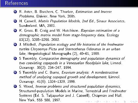
References
1 R. Aster, B. Borchers, C. Thurber, Estimation and InverseProblems, Elsivier, New York, 2005.
2 H. Caswell, Matrix Population Models, 2nd Ed., Sinaur Associates,Sunderland, MA, 2001.
3 K. Gross, B. Craig and W. Hutchison, Bayesian estimation of ademographic matrix model from stage-frequency data, Ecology83(12), 3285�3298, 2002.
4 J. Mitchell, Population ecology and life histories of the freshwaterturtles Chrysemys Picta and Sternotherus Odoratus in an urbanlake, Herpetological Monographs (2), 40�61, 1989.
5 S Twombly, Comparative demography and population dynamics oftwo coexisting copepods in a Venezuelan �oodplain lake, Limnol.Oceanogr. 39(2), 234�247, 1994.
6 S Twombly and C. Burns, Exuvium analysis: A nondestructivemethod of analyzing copepod growth and development, Limnol.Oceanogr. 41(6), 1324�1329, 1996.
7 S. Wood, Inverse problems and structured-population dynamics,Structured-population Models in Marine, Terrestrial and FreshwaterSystems (Ed. S. Tuljapurkar and J. Caswell), Chapman and Hall,New York, 555�586, 1997.
Basic Ideas and TheoryInverse ProblemsConclusionsThe Lefkowitz ModelMatrix Theory
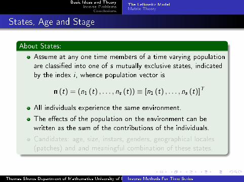
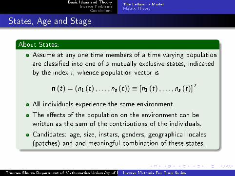
States, Age and Stage
About States:
Assume at any one time members of a time varying population
are classi�ed into one of s mutually exclusive states, indicated
by the index i , whence population vector is
n (t) = (n1 (t) , . . . , ns (t)) ≡ [n1 (t) , . . . , ns (t)]T
All individuals experience the same environment.
The e�ects of the population on the environment can be
written as the sum of the contributions of the individuals.
Candidates: age, size, instars, genders, geographical locales
(patches) and and meaningful combination of these states.
Thomas Shores Department of Mathematics University of NebraskaInverse Methods For Time Series
Basic Ideas and TheoryInverse ProblemsConclusionsThe Lefkowitz ModelMatrix Theory
States, Age and Stage
About States:
Assume at any one time members of a time varying population
are classi�ed into one of s mutually exclusive states, indicated
by the index i , whence population vector is
n (t) = (n1 (t) , . . . , ns (t)) ≡ [n1 (t) , . . . , ns (t)]T
All individuals experience the same environment.
The e�ects of the population on the environment can be
written as the sum of the contributions of the individuals.
Candidates: age, size, instars, genders, geographical locales
(patches) and and meaningful combination of these states.
Thomas Shores Department of Mathematics University of NebraskaInverse Methods For Time Series
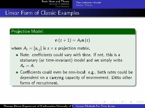
Basic Ideas and TheoryInverse ProblemsConclusionsThe Lefkowitz ModelMatrix Theory
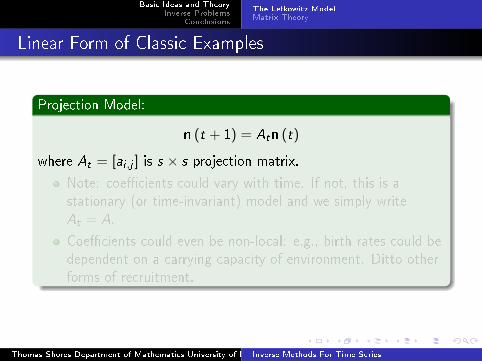
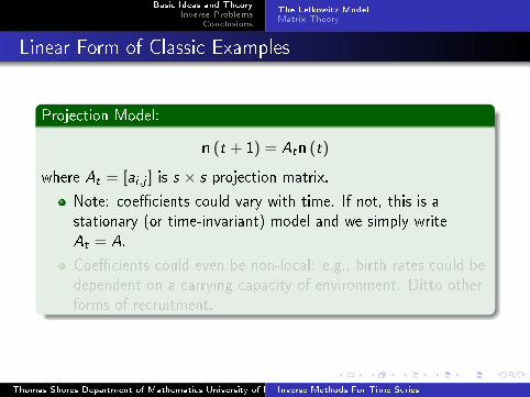
Linear Form of Classic Examples
Projection Model:
n (t + 1) = Atn (t)
where At = [ai ,j ] is s × s projection matrix.
Note: coe�cients could vary with time. If not, this is a
stationary (or time-invariant) model and we simply write
At = A.
Coe�cients could even be non-local: e.g., birth rates could be
dependent on a carrying capacity of environment. Ditto other
forms of recruitment.
Thomas Shores Department of Mathematics University of NebraskaInverse Methods For Time Series
Basic Ideas and TheoryInverse ProblemsConclusionsThe Lefkowitz ModelMatrix Theory
Linear Form of Classic Examples
Projection Model:
n (t + 1) = Atn (t)
where At = [ai ,j ] is s × s projection matrix.
Note: coe�cients could vary with time. If not, this is a
stationary (or time-invariant) model and we simply write
At = A.
Coe�cients could even be non-local: e.g., birth rates could be
dependent on a carrying capacity of environment. Ditto other
forms of recruitment.
Thomas Shores Department of Mathematics University of NebraskaInverse Methods For Time Series
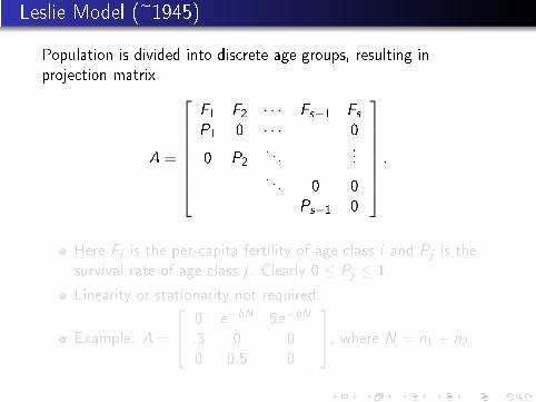
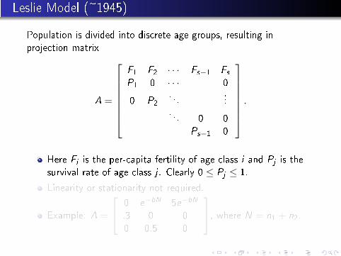
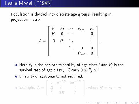
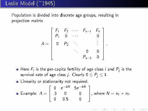
Leslie Model (~1945)
Population is divided into discrete age groups, resulting in
projection matrix
A =
F1 F2 · · · Fs−1 FsP1 0 · · · 0
0 P2. . .
.... . . 0 0
Ps−1 0
.
Here Fi is the per-capita fertility of age class i and Pj is the
survival rate of age class j . Clearly 0 ≤ Pj ≤ 1.
Linearity or stationarity not required.
Example: A =
0 e−bN 5e−bN
.3 0 0
0 0.5 0
, where N = n1 + n2.
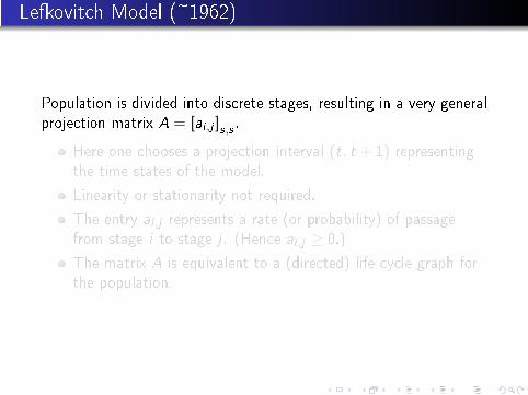
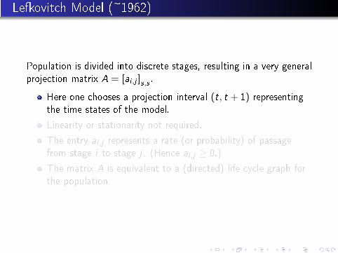
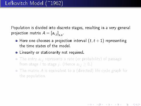
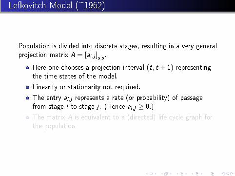
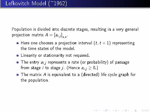
Lefkovitch Model (~1962)
Population is divided into discrete stages, resulting in a very general
projection matrix A = [ai ,j ]s,s .
Here one chooses a projection interval (t, t + 1) representingthe time states of the model.
Linearity or stationarity not required.
The entry ai ,j represents a rate (or probability) of passage
from stage i to stage j . (Hence ai ,j ≥ 0.)
The matrix A is equivalent to a (directed) life cycle graph for
the population.
Basic Ideas and TheoryInverse ProblemsConclusionsThe Lefkowitz ModelMatrix Theory
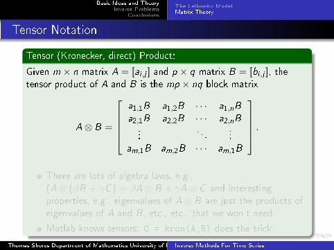
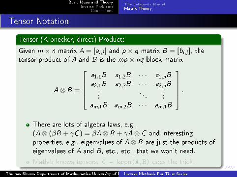
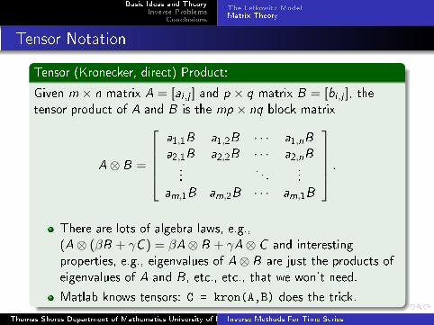
Tensor Notation
Tensor (Kronecker, direct) Product:
Given m × n matrix A = [ai ,j ] and p × q matrix B = [bi ,j ], thetensor product of A and B is the mp × nq block matrix
A⊗ B =
a1,1B a1,2B · · · a1,nB
a2,1B a2,2B · · · a2,nB...
. . ....
am,1B am,2B · · · am,1B
.
There are lots of algebra laws, e.g.,
(A⊗ (βB + γC ) = βA⊗ B + γA⊗ C and interesting
properties, e.g., eigenvalues of A⊗ B are just the products of
eigenvalues of A and B , etc., etc., that we won't need.
Matlab knows tensors: C = kron(A,B) does the trick.
Thomas Shores Department of Mathematics University of NebraskaInverse Methods For Time Series
Basic Ideas and TheoryInverse ProblemsConclusionsThe Lefkowitz ModelMatrix Theory
Tensor Notation
Tensor (Kronecker, direct) Product:
Given m × n matrix A = [ai ,j ] and p × q matrix B = [bi ,j ], thetensor product of A and B is the mp × nq block matrix
A⊗ B =
a1,1B a1,2B · · · a1,nB
a2,1B a2,2B · · · a2,nB...
. . ....
am,1B am,2B · · · am,1B
.
There are lots of algebra laws, e.g.,
(A⊗ (βB + γC ) = βA⊗ B + γA⊗ C and interesting
properties, e.g., eigenvalues of A⊗ B are just the products of
eigenvalues of A and B , etc., etc., that we won't need.
Matlab knows tensors: C = kron(A,B) does the trick.
Thomas Shores Department of Mathematics University of NebraskaInverse Methods For Time Series
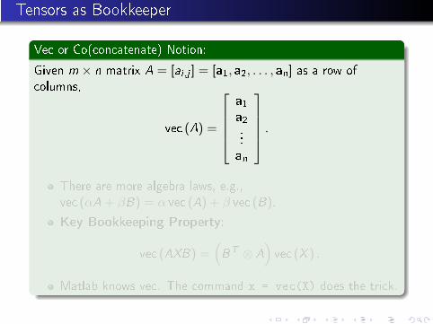
Tensors as Bookkeeper
Vec or Co(concatenate) Notion:
Given m × n matrix A = [ai ,j ] = [a1, a2, . . . , an] as a row of
columns,
vec (A) =
a1a2...
an
.
There are more algebra laws, e.g.,
vec (αA + βB) = α vec (A) + β vec (B).
Key Bookkeeping Property:
vec (AXB) =(BT ⊗ A
)vec (X ) .
Matlab knows vec. The command x = vec(X) does the trick.
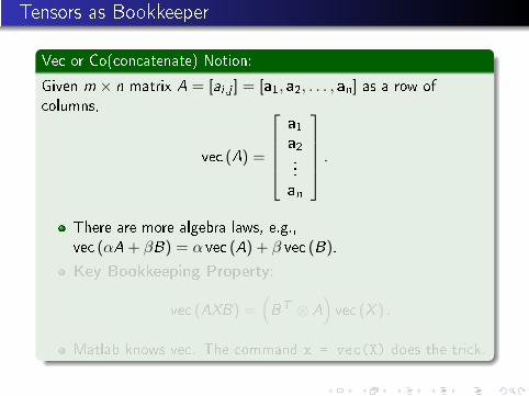
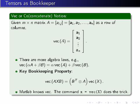
Basic Ideas and TheoryInverse ProblemsConclusionsFormulation and ExamplesSome Methodologies
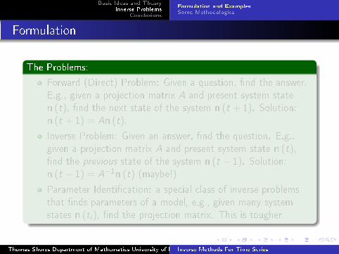
Formulation
The Problems:
Forward (Direct) Problem: Given a question, �nd the answer.
E.g., given a projection matrix A and present system state
n (t), �nd the next state of the system n (t + 1). Solution:n (t + 1) = An (t).
Inverse Problem: Given an answer, �nd the question. E.g.,
given a projection matrix A and present system state n (t),�nd the previous state of the system n (t − 1). Solution:n (t − 1) = A−1n (t) (maybe!)
Parameter Identi�cation: a special class of inverse problems
that �nds parameters of a model, e.g., given many system
states n (ti ), �nd the projection matrix. This is tougher.
Thomas Shores Department of Mathematics University of NebraskaInverse Methods For Time Series
Basic Ideas and TheoryInverse ProblemsConclusionsFormulation and ExamplesSome Methodologies
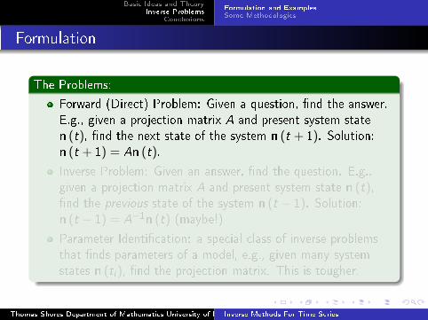
Formulation
The Problems:
Forward (Direct) Problem: Given a question, �nd the answer.
E.g., given a projection matrix A and present system state
n (t), �nd the next state of the system n (t + 1). Solution:n (t + 1) = An (t).
Inverse Problem: Given an answer, �nd the question. E.g.,
given a projection matrix A and present system state n (t),�nd the previous state of the system n (t − 1). Solution:n (t − 1) = A−1n (t) (maybe!)
Parameter Identi�cation: a special class of inverse problems
that �nds parameters of a model, e.g., given many system
states n (ti ), �nd the projection matrix. This is tougher.
Thomas Shores Department of Mathematics University of NebraskaInverse Methods For Time Series
Basic Ideas and TheoryInverse ProblemsConclusionsFormulation and ExamplesSome Methodologies
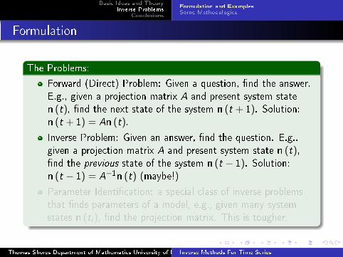
Formulation
The Problems:
Forward (Direct) Problem: Given a question, �nd the answer.
E.g., given a projection matrix A and present system state
n (t), �nd the next state of the system n (t + 1). Solution:n (t + 1) = An (t).
Inverse Problem: Given an answer, �nd the question. E.g.,
given a projection matrix A and present system state n (t),�nd the previous state of the system n (t − 1). Solution:n (t − 1) = A−1n (t) (maybe!)
Parameter Identi�cation: a special class of inverse problems
that �nds parameters of a model, e.g., given many system
states n (ti ), �nd the projection matrix. This is tougher.
Thomas Shores Department of Mathematics University of NebraskaInverse Methods For Time Series
Basic Ideas and TheoryInverse ProblemsConclusionsFormulation and ExamplesSome Methodologies
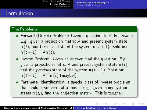
Formulation
The Problems:
Forward (Direct) Problem: Given a question, �nd the answer.
E.g., given a projection matrix A and present system state
n (t), �nd the next state of the system n (t + 1). Solution:n (t + 1) = An (t).
Inverse Problem: Given an answer, �nd the question. E.g.,
given a projection matrix A and present system state n (t),�nd the previous state of the system n (t − 1). Solution:n (t − 1) = A−1n (t) (maybe!)
Parameter Identi�cation: a special class of inverse problems
that �nds parameters of a model, e.g., given many system
states n (ti ), �nd the projection matrix. This is tougher.
Thomas Shores Department of Mathematics University of NebraskaInverse Methods For Time Series
Basic Ideas and TheoryInverse ProblemsConclusionsFormulation and ExamplesSome Methodologies
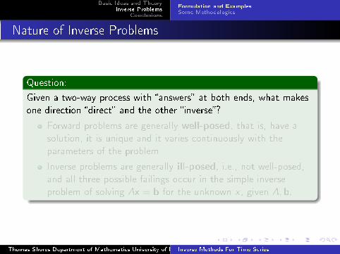
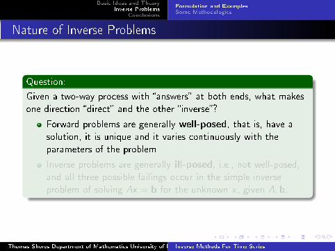
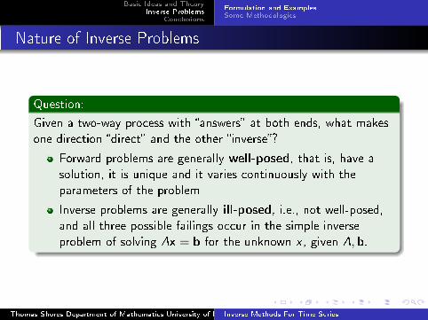
Nature of Inverse Problems
Question:
Given a two-way process with �answers� at both ends, what makes
one direction �direct� and the other �inverse�?
Forward problems are generally well-posed, that is, have a
solution, it is unique and it varies continuously with the
parameters of the problem
Inverse problems are generally ill-posed, i.e., not well-posed,
and all three possible failings occur in the simple inverse
problem of solving Ax = b for the unknown x , given A,b.
Thomas Shores Department of Mathematics University of NebraskaInverse Methods For Time Series
Basic Ideas and TheoryInverse ProblemsConclusionsFormulation and ExamplesSome Methodologies
Nature of Inverse Problems
Question:
Given a two-way process with �answers� at both ends, what makes
one direction �direct� and the other �inverse�?
Forward problems are generally well-posed, that is, have a
solution, it is unique and it varies continuously with the
parameters of the problem
Inverse problems are generally ill-posed, i.e., not well-posed,
and all three possible failings occur in the simple inverse
problem of solving Ax = b for the unknown x , given A,b.
Thomas Shores Department of Mathematics University of NebraskaInverse Methods For Time Series
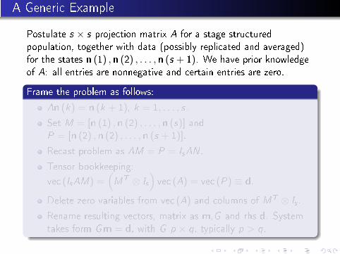
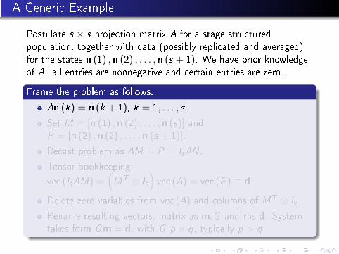
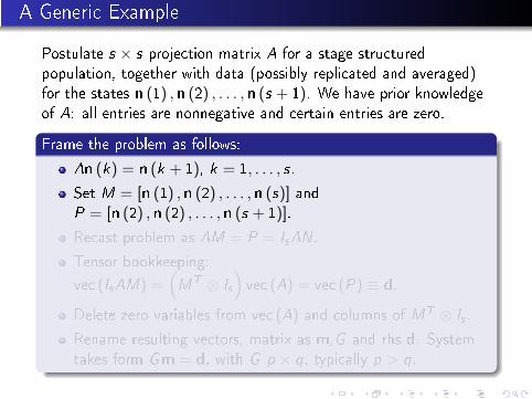
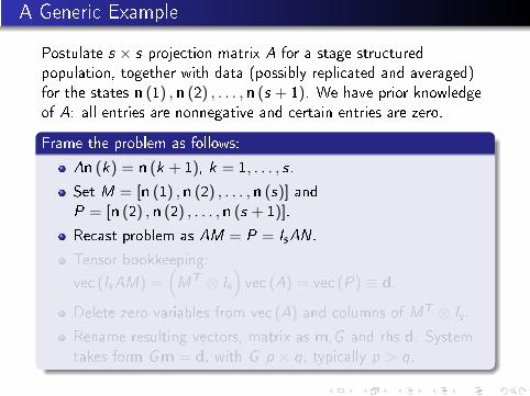
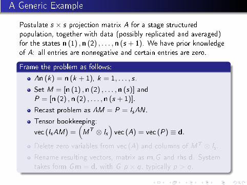
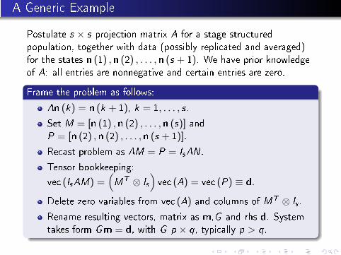
A Generic Example
Postulate s × s projection matrix A for a stage structured
population, together with data (possibly replicated and averaged)
for the states n (1) ,n (2) , . . . ,n (s + 1). We have prior knowledge
of A: all entries are nonnegative and certain entries are zero.
Frame the problem as follows:
An (k) = n (k + 1), k = 1, . . . , s.
Set M = [n (1) ,n (2) , . . . ,n (s)] andP = [n (2) ,n (2) , . . . ,n (s + 1)].
Recast problem as AM = P = IsAN.
Tensor bookkeeping:
vec (IsAM) =(MT ⊗ Is
)vec (A) = vec (P) ≡ d.
Delete zero variables from vec (A) and columns of MT ⊗ Is .
Rename resulting vectors, matrix as m,G and rhs d. System
takes form Gm = d, with G p × q, typically p > q.
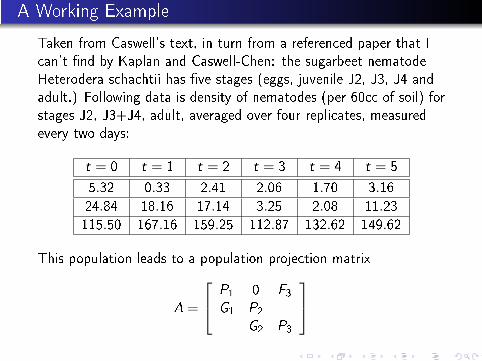
A Working Example
Taken from Caswell's text, in turn from a referenced paper that I
can't �nd by Kaplan and Caswell-Chen: the sugarbeet nematode
Heterodera schachtii has �ve stages (eggs, juvenile J2, J3, J4 and
adult.) Following data is density of nematodes (per 60cc of soil) for
stages J2, J3+J4, adult, averaged over four replicates, measured
every two days:
t = 0 t = 1 t = 2 t = 3 t = 4 t = 5
5.32 0.33 2.41 2.06 1.70 3.16
24.84 18.16 17.14 3.25 2.08 11.23
115.50 167.16 159.25 112.87 132.62 149.62
This population leads to a population projection matrix
A =
P1 0 F3G1 P2
G2 P3
Basic Ideas and TheoryInverse ProblemsConclusionsFormulation and ExamplesSome Methodologies
Least Squares (?)
Thomas Shores Department of Mathematics University of NebraskaInverse Methods For Time Series
Basic Ideas and TheoryInverse ProblemsConclusionsFormulation and ExamplesSome Methodologies
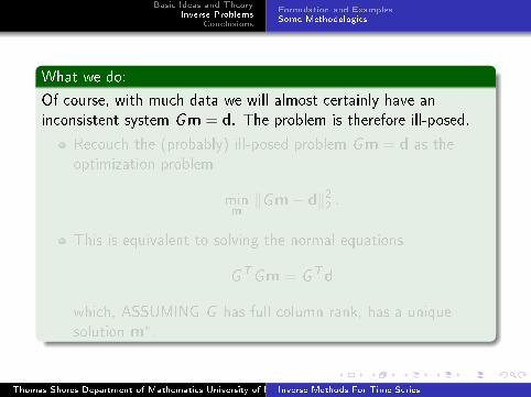
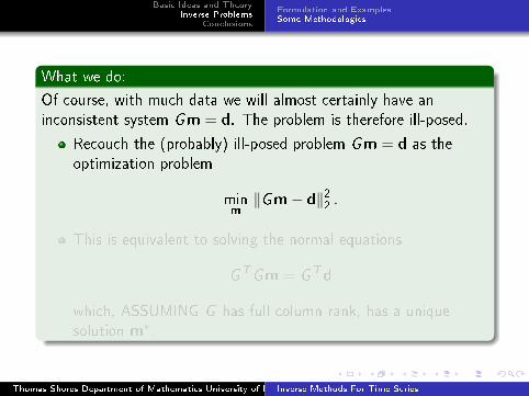
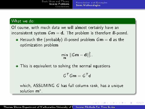
What we do:
Of course, with much data we will almost certainly have an
inconsistent system Gm = d. The problem is therefore ill-posed.
Recouch the (probably) ill-posed problem Gm = d as the
optimization problem
minm
‖Gm− d‖22 .
This is equivalent to solving the normal equations
GTGm = GTd
which, ASSUMING G has full column rank, has a unique
solution m∗.
Thomas Shores Department of Mathematics University of NebraskaInverse Methods For Time Series
Basic Ideas and TheoryInverse ProblemsConclusionsFormulation and ExamplesSome Methodologies
What we do:
Of course, with much data we will almost certainly have an
inconsistent system Gm = d. The problem is therefore ill-posed.
Recouch the (probably) ill-posed problem Gm = d as the
optimization problem
minm
‖Gm− d‖22 .
This is equivalent to solving the normal equations
GTGm = GTd
which, ASSUMING G has full column rank, has a unique
solution m∗.
Thomas Shores Department of Mathematics University of NebraskaInverse Methods For Time Series

Least Squares and Working Example
Basic Ideas and TheoryInverse ProblemsConclusionsFormulation and ExamplesSome Methodologies
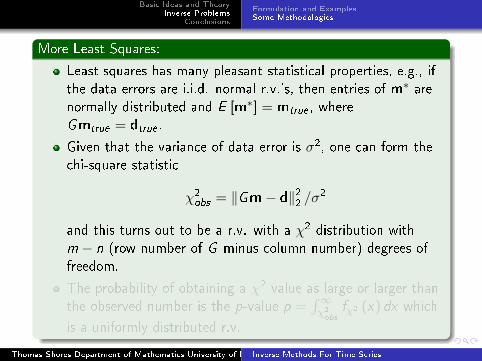
More Least Squares:
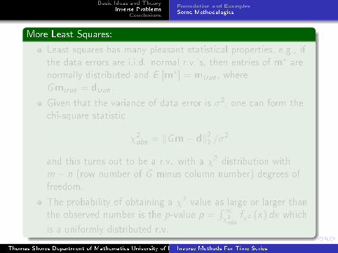
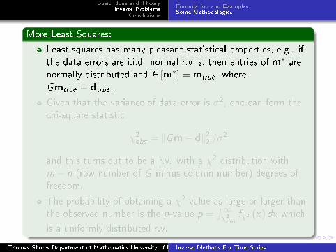
Least squares has many pleasant statistical properties, e.g., if
the data errors are i.i.d. normal r.v.'s, then entries of m∗ arenormally distributed and E [m∗] = mtrue , where
Gmtrue = dtrue .
Given that the variance of data error is σ2, one can form the
chi-square statistic
χ2obs = ‖Gm− d‖22 /σ2
and this turns out to be a r.v. with a χ2 distribution with
m − n (row number of G minus column number) degrees of
freedom.
The probability of obtaining a χ2 value as large or larger than
the observed number is the p-value p =∫∞χ2obs
fχ2 (x) dx which
is a uniformly distributed r.v.
Thomas Shores Department of Mathematics University of NebraskaInverse Methods For Time Series
Basic Ideas and TheoryInverse ProblemsConclusionsFormulation and ExamplesSome Methodologies
More Least Squares:
Least squares has many pleasant statistical properties, e.g., if
the data errors are i.i.d. normal r.v.'s, then entries of m∗ arenormally distributed and E [m∗] = mtrue , where
Gmtrue = dtrue .
Given that the variance of data error is σ2, one can form the
chi-square statistic
χ2obs = ‖Gm− d‖22 /σ2
and this turns out to be a r.v. with a χ2 distribution with
m − n (row number of G minus column number) degrees of
freedom.
The probability of obtaining a χ2 value as large or larger than
the observed number is the p-value p =∫∞χ2obs
fχ2 (x) dx which
is a uniformly distributed r.v.
Thomas Shores Department of Mathematics University of NebraskaInverse Methods For Time Series
Basic Ideas and TheoryInverse ProblemsConclusionsFormulation and ExamplesSome Methodologies
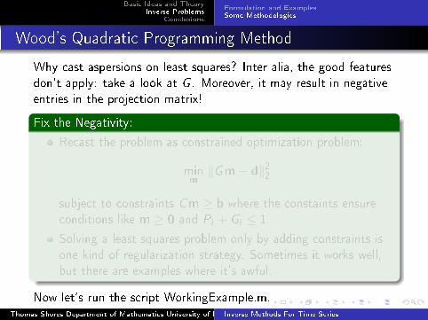
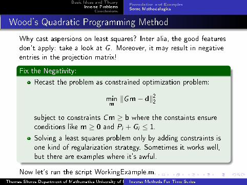
Wood's Quadratic Programming Method
Why cast aspersions on least squares? Inter alia, the good features
don't apply: take a look at G . Moreover, it may result in negative
entries in the projection matrix!
Fix the Negativity:
Recast the problem as constrained optimization problem:
minm
‖Gm− d‖22
subject to constraints Cm ≥ b where the constaints ensure
conditions like m ≥ 0 and Pi + Gi ≤ 1.
Solving a least squares problem only by adding constraints is
one kind of regularization strategy. Sometimes it works well,
but there are examples where it's awful.
Now let's run the script WorkingExample.m.Thomas Shores Department of Mathematics University of NebraskaInverse Methods For Time Series
Basic Ideas and TheoryInverse ProblemsConclusionsFormulation and ExamplesSome Methodologies
Regularized Least Squares
Thomas Shores Department of Mathematics University of NebraskaInverse Methods For Time Series

Basic Ideas and TheoryInverse ProblemsConclusionsFormulation and ExamplesSome Methodologies
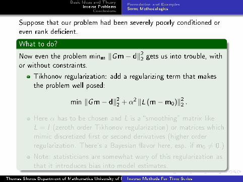
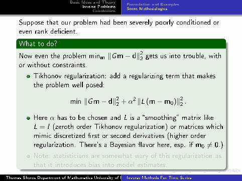
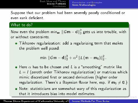
Suppose that our problem had been severely poorly conditioned or
even rank de�cient.
What to do?
Now even the problem minm ‖Gm− d‖22 gets us into trouble, with
or without constraints.
Tikhonov regularization: add a regularizing term that makes
the problem well posed:
min ‖Gm− d‖22 + α2 ‖L (m−m0)‖22 .
Here α has to be chosen and L is a �smoothing� matrix like
L = I (zeroth order Tikhonov regularization) or matrices which
mimic discretized �rst or second derivatives (higher order
regularization. There's a Bayesian �avor here, esp. if m0 6= 0.)
Note: statisticians are somewhat wary of this regularization as
that it introduces bias into model estimates.
Thomas Shores Department of Mathematics University of NebraskaInverse Methods For Time Series
Basic Ideas and TheoryInverse ProblemsConclusionsFormulation and ExamplesSome Methodologies
Suppose that our problem had been severely poorly conditioned or
even rank de�cient.
What to do?
Now even the problem minm ‖Gm− d‖22 gets us into trouble, with
or without constraints.
Tikhonov regularization: add a regularizing term that makes
the problem well posed:
min ‖Gm− d‖22 + α2 ‖L (m−m0)‖22 .
Here α has to be chosen and L is a �smoothing� matrix like
L = I (zeroth order Tikhonov regularization) or matrices which
mimic discretized �rst or second derivatives (higher order
regularization. There's a Bayesian �avor here, esp. if m0 6= 0.)
Note: statisticians are somewhat wary of this regularization as
that it introduces bias into model estimates.
Thomas Shores Department of Mathematics University of NebraskaInverse Methods For Time Series

Basic Ideas and TheoryInverse ProblemsConclusionsFormulation and ExamplesSome Methodologies
Determination of α
Thomas Shores Department of Mathematics University of NebraskaInverse Methods For Time Series

Basic Ideas and TheoryInverse ProblemsConclusionsFormulation and ExamplesSome Methodologies
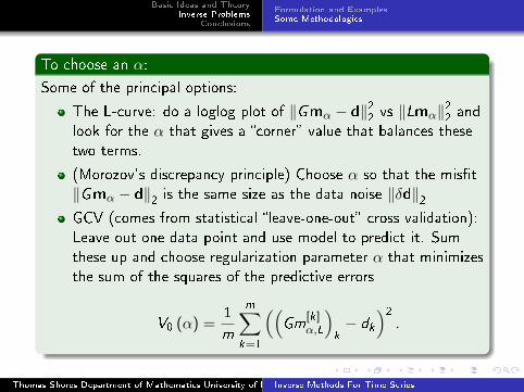
To choose an α:
Some of the principal options:
The L-curve: do a loglog plot of ‖Gmα − d‖22 vs ‖Lmα‖22 and
look for the α that gives a �corner� value that balances these
two terms.
(Morozov's discrepancy principle) Choose α so that the mis�t
‖Gmα − d‖2 is the same size as the data noise ‖δd‖2GCV (comes from statistical �leave-one-out� cross validation):
Leave out one data point and use model to predict it. Sum
these up and choose regularization parameter α that minimizes
the sum of the squares of the predictive errors
V0 (α) =1
m
m∑k=1
((Gm
[k]α,L
)k− dk
)2.
Thomas Shores Department of Mathematics University of NebraskaInverse Methods For Time Series

Basic Ideas and TheoryInverse ProblemsConclusionsFormulation and ExamplesSome Methodologies
To choose an α:
Some of the principal options:
The L-curve: do a loglog plot of ‖Gmα − d‖22 vs ‖Lmα‖22 and
look for the α that gives a �corner� value that balances these
two terms.
(Morozov's discrepancy principle) Choose α so that the mis�t
‖Gmα − d‖2 is the same size as the data noise ‖δd‖2GCV (comes from statistical �leave-one-out� cross validation):
Leave out one data point and use model to predict it. Sum
these up and choose regularization parameter α that minimizes
the sum of the squares of the predictive errors
V0 (α) =1
m
m∑k=1
((Gm
[k]α,L
)k− dk
)2.
Thomas Shores Department of Mathematics University of NebraskaInverse Methods For Time Series
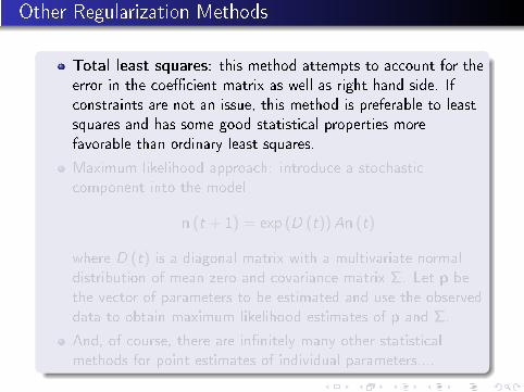
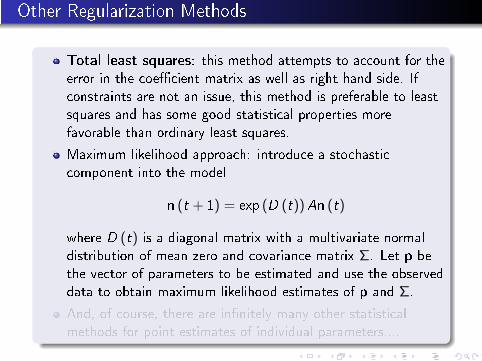
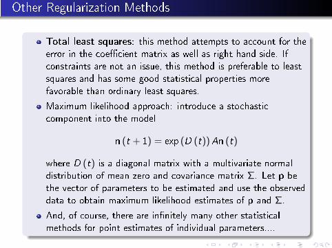
Other Regularization Methods
Total least squares: this method attempts to account for the
error in the coe�cient matrix as well as right hand side. If
constraints are not an issue, this method is preferable to least
squares and has some good statistical properties more
favorable than ordinary least squares.
Maximum likelihood approach: introduce a stochastic
component into the model
n (t + 1) = exp (D (t))An (t)
where D (t) is a diagonal matrix with a multivariate normal
distribution of mean zero and covariance matrix Σ. Let p be
the vector of parameters to be estimated and use the observed
data to obtain maximum likelihood estimates of p and Σ.
And, of course, there are in�nitely many other statistical
methods for point estimates of individual parameters....
Basic Ideas and TheoryInverse ProblemsConclusions
Summary
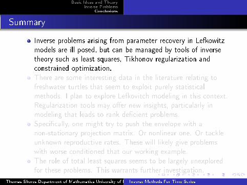
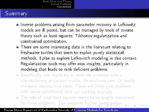
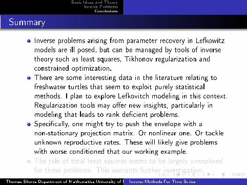
Inverse problems arising from parameter recovery in Lefkowitz
models are ill posed, but can be managed by tools of inverse
theory such as least squares, Tikhonov regularization and
constrained optimization.
There are some interesting data in the literature relating to
freshwater turtles that seem to exploit purely statistical
methods. I plan to explore Lefkovitch modeling in this context.
Regularization tools may o�er new insights, particularly in
modeling that leads to rank de�cient problems.
Speci�cally, one might try to push the envelope with a
non-stationary projection matrix. Or nonlinear one. Or tackle
unknown reproductive rates. These will likely give problems
with worse conditioned that our working example.
The role of total least squares seems to be largely unexplored
for these problems. This warrants further investigation.
Thomas Shores Department of Mathematics University of NebraskaInverse Methods For Time Series
Basic Ideas and TheoryInverse ProblemsConclusions
Summary
Inverse problems arising from parameter recovery in Lefkowitz
models are ill posed, but can be managed by tools of inverse
theory such as least squares, Tikhonov regularization and
constrained optimization.
There are some interesting data in the literature relating to
freshwater turtles that seem to exploit purely statistical
methods. I plan to explore Lefkovitch modeling in this context.
Regularization tools may o�er new insights, particularly in
modeling that leads to rank de�cient problems.
Speci�cally, one might try to push the envelope with a
non-stationary projection matrix. Or nonlinear one. Or tackle
unknown reproductive rates. These will likely give problems
with worse conditioned that our working example.
The role of total least squares seems to be largely unexplored
for these problems. This warrants further investigation.
Thomas Shores Department of Mathematics University of NebraskaInverse Methods For Time Series
![Bibliography - University of British Columbiahoos/SLS-Internal/bib.pdf · 372 BIBLIOGRAPHY [Borchers and Furman, 1999] B. Borchers and J. Furman. A two-phase ex-act algorithmfor MAX-SAT](https://img.pdfslide.us/doc/110x75/5ed3851e2c6992453d414430/bibliography-university-of-british-columbia-hoossls-internalbibpdf-372-bibliography.jpg)