NOTES ON FEYNMAN INTEGRALS AND RENORMALIZATION ON FEYNMAN INTEGRALS AND RENORMALIZATION 3 2. FEYNMAN GRAPHS AND FEYNMAN INTEGRALS For the purpose of this paper, a Feynman graph is

arX

iv:1

005.

3960

v1 [

hep-

th]

21 M

ay 2

010

NOTES ON FEYNMAN INTEGRALS AND RENORMALIZATION

CHRISTOPH BERGBAUER

ABSTRACT. I review various aspects of Feynman integrals, regularization andrenormalization. Following Bloch, I focus on a linear algebraic approach to theFeynman rules, and I try to bring together several renormalization methods foundin the literature from a unifying point of view, using resolutions of singularities.In the second part of the paper, I briefly sketch the work of Belkale, Brosnanresp. Bloch, Esnault and Kreimer on the motivic nature of Feynman integrals.

CONTENTS

1. Introduction 12. Feynman graphs and Feynman integrals 33. Regularization and renormalization 144. Motives and residues of Feynman graphs 28References 36

1. INTRODUCTION

In recent years there has been a growing interest in Feynman graphs and theirintegrals.

Physicists use Feynman graphs and the associated integralsin order to com-pute certain experimentally measurable quantities out of quantum field theories.The problem is that there are conceptual difficulties in the definition of interact-ing quantum field theories in four dimensions. The good thingis that nonethelessthe Feynman graph formalism is very successful in the sense that the quantitiesobtained from it match with the quantities obtained in experiment extremely well.Feynman graphs are interpreted as elements of a perturbation theory, i. e. as anexpansion of an (interesting) interacting quantum field theory in the neighborhoodof a (simple) free quantum field theory. One therefore hopes that a better under-standing of Feynman graphs and their integrals could eventually lead to a betterunderstanding of the true nature of quantum field theories, and contribute to someof the longstanding open questions in the field.

Date: May 20, 2010.Key words and phrases.Feynman graph, Feynman integral, Feynman rules, regularization, renor-

malization, subspace arrangement, resolution of singularities, Connes-Kreimer Hopf algebra, ma-troid, multiple zeta value, motive, period.

1

http://arxiv.org/abs/1005.3960v1

2 CHRISTOPH BERGBAUER

A Feynman graph is simply a finite graph, to which one associates a certainintegral: The integrand depends on the quantum field theory in question, but in thesimplest case it is just the inverse of a direct product of rank 4 quadratic forms, onefor each edge of the graph, restricted to a real linear subspace determined by thetopology of the graph.

For a general graph, there is currently no canonical way of solving this integralanalytically. However, in this simple case where the integrand is algebraic, onecan be convinced to regard the integral as a period of a mixed motive, another no-tion which is not rigorously defined as of today. All these Feynman periods thathave been computed so far, are rational linear combinationsof multiple zeta val-ues, which are known to be periods of mixed Tate motives, a simpler, and betterunderstood kind of motives. A stunning theorem of Belkale and Brosnan howeverindicates that this is possibly a coincidence due to the relatively small number ofFeynman periods known today: They showed that in fact any algebraic variety de-fined overZ is related to a Feynman graph hypersurface (the Feynman period isone period of the motive of this hypersurface) in a quite obscure way.

The purpose of this paper is to review selected aspects of Feynman graphs, Feyn-man integrals and renormalization in order to discuss some of the recent work byBloch, Esnault, Kreimer and others on the motivic nature of these integrals. It isbased on public lectures given at the ESI in March 2009, at theDESY and IHES inApril and June 2009, and several informal lectures in a localseminar in Mainz infall and winter 2009. I would like to thank the other participants for their lecturesand discussions.

Much of my approach is centered around the notion of renormalization, whichseems crucial for a deeper understanding of Quantum Field Theory. No claim oforiginality is made except for section 3.2 and parts of the surrounding sections,which is a review of my own research with R. Brunetti and D. Kreimer [10], andsection 3.6 which contains new results.

This paper is not meant to be a complete and up to date survey byany means. Inparticular, several recent developments in the area, for example the work of Brown[24, 25], Aluffi and Marcolli [1–3], Doryn and Schnetz [35, 75], and the theory ofConnes and Marcolli [32] are not covered here.

Acknowledgements.I thank S. Muller-Stach, R. Brunetti, S. Bloch, M. Kontsevich,P. Brosnan, E. Vogt, C. Lange, A. Usnich, T. Ledwig, F. Brown and especiallyD. Kreimer for discussion on the subject of this paper. I would like to thank theESI and the organizers of the spring 2009 program on number theory and physicsfor hospitality during the month of March 2009, and the IHES for hospitality inJanuary and February 2010. My research is funded by the SFB 45of the DeutscheForschungsgemeinschaft.

NOTES ON FEYNMAN INTEGRALS AND RENORMALIZATION 3

2. FEYNMAN GRAPHS AND FEYNMAN INTEGRALS

For the purpose of this paper, a Feynman graph is simply a finite connectedmultigraph where ”multi” means that there may be several, parallel edges betweenvertices. Loops, i. e. edges connecting to the same vertex atboth ends, are notallowed in this paper. Roughly, physicists think of edges asvirtual particles and ofvertices as interactions between the virtual particles corresponding to the adjacentedges.

If one has to consider several types of particles, one has several types (colors,shapes etc.) of edges.

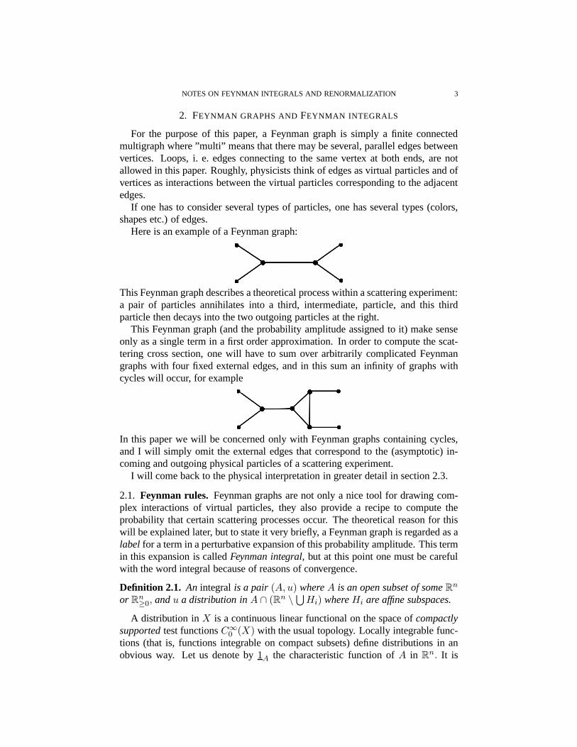
Here is an example of a Feynman graph:

This Feynman graph describes a theoretical process within ascattering experiment:a pair of particles annihilates into a third, intermediate,particle, and this thirdparticle then decays into the two outgoing particles at the right.

This Feynman graph (and the probability amplitude assignedto it) make senseonly as a single term in a first order approximation. In order to compute the scat-tering cross section, one will have to sum over arbitrarily complicated Feynmangraphs with four fixed external edges, and in this sum an infinity of graphs withcycles will occur, for example

In this paper we will be concerned only with Feynman graphs containing cycles,and I will simply omit the external edges that correspond to the (asymptotic) in-coming and outgoing physical particles of a scattering experiment.

I will come back to the physical interpretation in greater detail in section 2.3.

2.1. Feynman rules. Feynman graphs are not only a nice tool for drawing com-plex interactions of virtual particles, they also provide arecipe to compute theprobability that certain scattering processes occur. The theoretical reason for thiswill be explained later, but to state it very briefly, a Feynman graph is regarded as alabel for a term in a perturbative expansion of this probability amplitude. This termin this expansion is calledFeynman integral, but at this point one must be carefulwith the word integral because of reasons of convergence.

Definition 2.1. An integralis a pair (A, u) whereA is an open subset of someRn

or Rn≥0, andu a distribution inA ∩ (Rn \

⋃Hi) whereHi are affine subspaces.

A distribution inX is a continuous linear functional on the space ofcompactlysupportedtest functionsC∞

0 (X) with the usual topology. Locally integrable func-tions (that is, functions integrable on compact subsets) define distributions in anobvious way. Let us denote by1A the characteristic function ofA in Rn. It is


certainly not a test function unlessA is compact, but ifu allows (decays rapidlyenough at∞), then we may evaluateu against1A. We writeu[f ] for the distribu-tion applied to the test functionf. If u is given by a locally integrable function, wemay also write

∫u(x)f(x)dx.

If u is given by a function which is integrable in all ofA, then(A, u) can beassociated with the usual integral

∫A u(x)dx = u[1A]. Feynman integrals however

are very often divergent: This means by definition that∫A u(x)dx is divergent, and

this can either result from problems with local integrability at theHi or lack ofintegrability at∞ away from theHi (if A is unbounded), or both. (A more unifiedpoint of view would be to start with aPn instead ofRn in order to have the diver-gence at∞ as a divergence at the hyperplaneH∞ at∞, but I will not exploit thishere).

A basic example for such a divergent integral is the pairA = R \ 0 andu(x) = |x|−1. The functionu is locally integrable insideA, hence a distributionin A. But neither is it integrable as|x| → ∞, nor locally integrable at0. Wewill see in a moment that the divergent Feynman integrals to be defined are higher-dimensional generalizations of this example, with an interesting arrangement oftheHi.

The following approach, which I learned from S. Bloch [14, 15], is quite pow-erful when one wants to understand the various Feynman rulesfrom a commonpoint of view. It is based on the idea that a Feynman graph firstdefines a pointconfiguration in someRn, and it is only this point configuration which determinesthe Feynman integral via the Feynman rules.

Let Γ be a Feynman graph with set of edgesE(Γ) and set of verticesV (Γ). Asubgraphγ has by definition the same vertex setV (γ) = V (Γ) butE(γ) ⊆ E(Γ).Impose temporarily an orientation of the edges, such that every edge has an in-comingve,in and an outgoing vertexve,out. Since we do not allow loops, the twoare different. Set(v : e) = 1 if v is the outgoing vertex ofe, (v : e) = −1 if vis the incoming vertex ande, and (v : e) = 0 otherwise. LetM = Rd, whered ∈ 2+ 2N, calledspace-time, with euclidean metric| · |. We will mostly considerthe case whered = 4, but it is useful to see the explicit dependence ond in theformulas.

All the information ofΓ is encoded in the map

ZE(Γ) ∂→ ZV (Γ)

sending an edgee ∈ E(Γ) to ∂(e) =∑

v∈V (Γ)(v : e)v = ve,out − ve,in. Thisis nothing but the chain complex for the oriented simplicialhomology of the 1-dimensional simplicial complexΓ, and it is a standard construction to build fromthis map∂ an exact sequence

(1) 0 → H1(Γ;Z) → ZE(Γ) ∂→ ZV (Γ) → H0(Γ;Z) → 0.


Like this one obtains two inclusions of free abelian groups intoZE(Γ) :

iΓ : H1(Γ;Z) → ZE(Γ)

The second one is obtained by dualizing

jΓ : ZV (Γ)∨/H0(Γ;Z)∂∨

→ ZE(Γ)∨.

Here, and generally whenever a basis is fixed, we can canonically identify freeabelian groups with their duals.

All this can be tensored withR, and we get inclusionsiΓ, jΓ of vector spacesinto another vector space with afixed basis.If one then replaces anyRn by Mn

and denotesi⊕dΓ = (iΓ, . . . , iΓ), j

⊕dΓ = (jΓ, . . . , jΓ), then two types of Feynman

integrals(A, u) are defined as follows:

AM = H1(Γ;R)d, uMΓ = (i⊕d

Γ )∗u⊗|E(Γ)|0,M ,

AP = MV (Γ)∨/H0(Γ;R)d, uPΓ = (j⊕dΓ )∗u

⊗|E(Γ)|0,P .

The distributionsu0,M , u0,P ∈ D′(M) therein are calledmomentum spaceresp.position space propagators. Several examples of propagators and how they arerelated will be discussed in the next section, but for a first reading

u0,M (p) =1

|p|2, u0,P (x) =

1

|x|d−2,

inverse powers of a rankd quadratic form. As announced earlier, the pullbacks(i⊕dΓ )∗u

⊗|E(Γ)|0,M and(j⊕d

Γ )∗u⊗|E(Γ)|0,M are only defined as distributions outside certain

affine spacesHi, that is for test functions supported on compact subsets which donot meet theseHi.

The map

Γ 7→ (AM , uMΓ )

is calledmomentum space Feynman rules, and the map

Γ 7→ (AP , uPΓ )

is calledposition space Feynman rules.

Usually, in the physics literature, the restriction to the subspace is imposed bymultiplying the direct product of propagators with severaldelta distributions whichare interpreted as ”momentum conservation” at each vertex in the momentum spacepicture, and dually ”translation invariance” in the position space case.

In position space, it is immediately seen that

uPΓ = (j⊕dΓ )∗u

⊗|E(Γ)|0,P = π∗

∏

e∈E(Γ)

u0,P (xe,out − xe,in)


whereπ∗ means pushforward along the projectionπ :MV (Γ)∨ →MV (Γ)∨/H0(Γ)d.[10].

In momentum space, things are a bit more complicated.

Definition 2.2. A connected graphΓ is calledcoreif rkH1(Γ \ e) < rkH1(Γ)for all e ∈ E(Γ).

By Euler’s formula (which follows from the exactness of (1))

rkH1(Γ)− |E(Γ)|+ |V (Γ)| − rkH0(Γ) = 0,

it is equivalent for a connected graphΓ to be core and to be one-particle-irreducible(1PI), a physicists’ notion:Γ is one-particle-irreducible if removing an edge doesnot disconnectΓ.

Let nowΓ be connected and core, then

uMΓ = (i⊕dΓ )∗u

⊗|E(Γ)|0,M =

∏

e∈E(Γ)

u0,M (pe)∏

v∈V (Γ)

δ0(∑

e∈E(Γ)

(v : e)pe).

This is simply becauseim iΓ = ker ∂, and because for

∂(∑

e∈E(Γ)

pee) =∑

e∈E(Γ)

pe∑

v

(v : e)v = 0

it is necessary that∑

e∈E(Γ)

(v : e)pe = 0 for all v ∈ V (Γ).

(The requirement thatΓ be core is really needed here because otherwise certaine ∈ E(Γ) would never show up in a cycle, and hence would be missing inside thedelta function.)

Moreover, one can define a version ofuMΓ which depends additionally onexter-nal momentaPv ∈ M, one for eachv ∈ V (Γ), up to momentum conservation foreach component

∑v∈C Pv = 0 :

(2) UMΓ (Pvv∈V (Γ)) =

∏

e∈E(Γ)

u0,M (pe)∏

v∈V (Γ)

δ0(Pv +∑

e∈E(Γ)

(v : e)pe).

By a slight abuse of notation I keep thePv, v ∈ V (Γ), as coordinate vectors forM|V (Γ)|/H0(Γ,R)d = AP and identify distributions onAP with distributions onM|V (Γ)| that are multiples of

∏C δ0(

∑v∈C Pv).

UMΓ is now a distribution on a subset ofAP ×AM , and

UMΓ |Pv=0,v∈V (Γ) = uMΓ .

The vectors inPv ∈ AP determine a shift of the linear subspaceAM = H1(Γ;R)⊕d →

M|E(Γ)| to an affine one. Usually all but a few of thePv are set to zero, namely allbut those which correspond to the incoming or outgoing particles of an experiment


(see section 2.3).

The relation between the momentum space and position space distributions isthen a Fourier duality. I denote byF the Fourier transform.

Proposition 2.1. If the basic propagators are Fourier-dual(Fu0,P = u0,M ), as isthe case foru0,M(p) = 1

|p|2 andu0,P (x) = 1|x|d−2 , then

(UMΓ [1AM

])(Pv) = FuPΓ

where only the (internal) momenta ofAM are integrated out; and this holds up toconvergence issues only, i. e. in the sense of Definition 2.1.

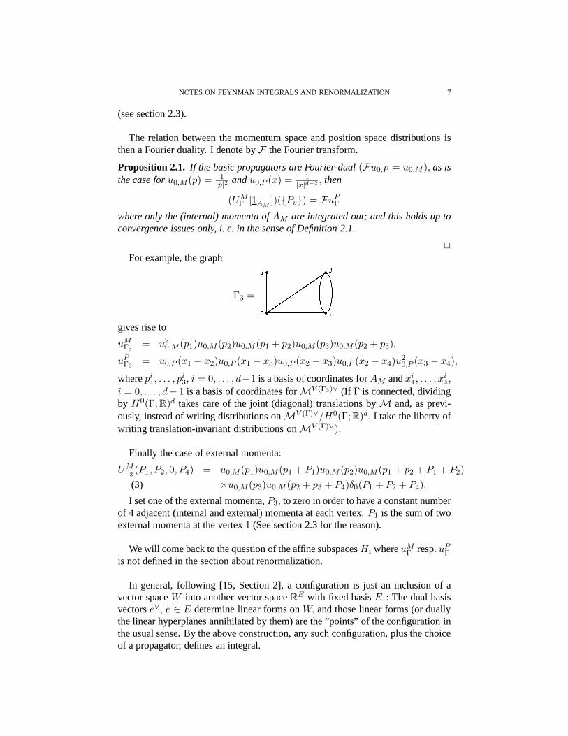
For example, the graph

Γ3 =

gives rise to

uMΓ3= u20,M (p1)u0,M (p2)u0,M (p1 + p2)u0,M (p3)u0,M (p2 + p3),

uPΓ3= u0,P (x1 − x2)u0,P (x1 − x3)u0,P (x2 − x3)u0,P (x2 − x4)u

20,P (x3 − x4),

wherepi1, . . . , pi3, i = 0, . . . , d−1 is a basis of coordinates forAM andxi1, . . . , x

i4,

i = 0, . . . , d− 1 is a basis of coordinates forMV (Γ3)∨ (If Γ is connected, dividingby H0(Γ;R)d takes care of the joint (diagonal) translations byM and, as previ-ously, instead of writing distributions onMV (Γ)∨/H0(Γ;R)d, I take the liberty ofwriting translation-invariant distributions onMV (Γ)∨).

Finally the case of external momenta:

UMΓ3(P1, P2, 0, P4) = u0,M (p1)u0,M (p1 + P1)u0,M (p2)u0,M (p1 + p2 + P1 + P2)

×u0,M (p3)u0,M (p2 + p3 + P4)δ0(P1 + P2 + P4).(3)

I set one of the external momenta,P3, to zero in order to have a constant numberof 4 adjacent (internal and external) momenta at each vertex: P1 is the sum of twoexternal momenta at the vertex1 (See section 2.3 for the reason).

We will come back to the question of the affine subspacesHi whereuMΓ resp.uPΓis not defined in the section about renormalization.

In general, following [15, Section 2], a configuration is just an inclusion of avector spaceW into another vector spaceRE with fixed basisE : The dual basisvectorse∨, e ∈ E determine linear forms onW, and those linear forms (or duallythe linear hyperplanes annihilated by them) are the ”points” of the configuration inthe usual sense. By the above construction, any such configuration, plus the choiceof a propagator, defines an integral.


If the configuration comes from a Feynman graph, the integralis calledFeynmanintegral.

2.2. Parametric representation. Integrals can be rewritten in many ways, usinglinearity of the integrand, of the domain, change of variables and Stokes’ theorem,and possibly a number of other tricks.

For many purposes it will be useful to have a version of the Feynman rules witha domainA which is much lower-dimensional than in the previous section buthas boundaries and corners. The first part of the basic trick here is to rewrite thepropagator

u0 =

∫ ∞

0exp(−aeu

−10 )dae

(whenever the choice of propagator allows this inversion;u0(p) = 1|p|2

certainly

does), introducing a new coordinateae ∈ R≥0 for each edgee ∈ E(Γ). Like thisone has a distribution

(4)⊗

e∈E(Γ)

exp(−aeu−10 (pe)) = exp

−

∑

e∈E(Γ)

aeu−10 (pe)

in (M × R≥0)|E(Γ)|. From now on I assumeu0(p) = 1

|p|2. Supposei : W →

R|E(Γ)| is an inclusion. Once a basis ofW is fixed, the linear forme∨i is a rowvector inW and its transpose(e∨i)t a column vector inW. The product(e∨i)t(e∨i)is then adimW -square matrix. Pulling back (4) along an inclusioni⊕d : W →M|E(Γ)| (such asi⊕d = i⊕d

Γ or i⊕d = j⊕dΓ ) means imposing linear relations on

thepe. These relations can be transposed onto theae : After integrating gaussianintegrals overW (this is the second part of the trick) and a change of variables, oneis left with the distribution

uSΓ(ae) =

det

∑

e∈E(Γ)

ae(e∨i)t(e∨i)

−d/2

onAS = R|E(Γ)|≥0 except certain intersectionsHi of coordinate hyperplanesae =

0. I discarded a multiplicative constantCΓ = (2π)d dimW/2 which does not de-pend on the topology of the graph.

Suppose thatd = 4. Depending on whetheri = iΓ or jΓ there is a momentumspace and a position space version of this trick. The two are dual to each other inthe following sense:

det∑

e∈E(Γ)

ae(e∨iΓ)

t(e∨iΓ) =

∏

e∈E(Γ)

ae

det

∑

e∈E(Γ)

a−1e (e∨jΓ)

t(e∨jΓ)

See [15, Proposition 1.6] for a proof. In this paper, we will only consider themomentum space version, wherei = iΓ. The map

Γ 7→ (AS , uSΓ)


with i = iΓ is calledSchwingeror parametric Feynman rules. Just as in the previ-ous section, there is also a version with external momenta which I just quote from[14,16,47]:

USΓ (ae, Pv) =

exp(−(N−1P )tP )(det

∑e∈E(Γ) ae(e

∨iΓ)t(e∨iΓ))2

where

N =∑

e∈E(Γ)

a−1e (e∨jΓ)

t(e∨jΓ),

ad(|V (Γ)| − dimH0(Γ;R))-square matrix.

The determinant

ΨΓ(ae) = det∑

e∈E(Γ)

ae(e∨iΓ)

t(e∨iΓ)

is a very special polynomial in theae. It is calledfirst graph polynomial, Kirchhoffpolynomialor Symanzik polynomial. It can be rewritten

(5) ΨΓ(ae) =∑

T sf of Γ

∏

e 6∈E(T )

ae

as a sum overspanning forestsT of Γ : A spanning forest is a subgraphE(T ) ⊆E(Γ) such that the map∂|RE(T ) : RE(T ) → RV (Γ)/H0(Γ;R) is an isomorphism;in other words, a subgraph without cycles that has exactly the same components asΓ. (In the special case whereΓ is connected, a spanning forest is called aspanningtreeand is characterized by being connected as well and having nocycles.)

For thesecond graph polynomialΦΓ, which is a polynomial in theae and aquadratic form in thePv , let us assume for simplicity thatΓ is connected. Then

ΦΓ(ae, Pv) = ΨΓ · (N−1P )tP =∑

T st of Γ

∑

e0∈E(T )

P t1P2ae0

∏

e 6∈E(T )

ae

wherePA =∑

v∈CAPv is the sum of momenta in the first connected component

CA andPB =∑

v∈CBPv the sum of momenta in the second connected compo-

nentCB of the graphE(T ) \ e0 (which has exactly two components sinceT isa spanning tree). See [15,16,47] for proofs.

Here is a simple example: If

Γ2 =


then

ΨΓ2 = a1 + a2

ΦΓ2 = P 21 a1a2

and

USΓ =

exp(−P 2

1a1a2a1+a2

)

(a1 + a2)2.

All this holds if u0,M = 1|p|2

. If u0,M = 1|p|2+m2 then

USΓ = exp(−m2

∑

e∈E(Γ)

ae)USΓ |m=0.

2.3. The origin of Feynman graphs in physics.Before we continue with a closeranalysis of the divergence locus of these Feynman integrals, it will be useful tohave at least a basic understanding of why they were introduced in physics. See[28, 33, 42, 45, 54, 72, 86, 87], for a general exposition, andI follow in particular[42, 72] in this section. Quantum Field Theory is a theory of particles which obeythe basic principles of quantum mechanics and special relativity at the same time.Special relativity is essentially the study of the Poincar´e group

P = R1,3 ⋊ SL(2,C)

(whereSL(2,C) → O(1, 3)+ is the universal double cover of the identity com-ponentO(1, 3)+ of O(1, 3)). In other words,P is the double cover of the groupof (space- and time-) orientation-preserving isometries of Minkowski space-timeR1,3 (I assumed = 4 in this section).

On the other hand, quantum mechanics always comes with a Hilbert space, avacuum vector, and operators on the Hilbert space.

By definition, asingle particleis then an irreducible unitary representation ofPon some Hilbert spaceH1. Those have been classified by Wigner according to thejoint spectrum ofP = (P0, . . . , P3), the vector of infinitesimal generators of thetranslations: Its joint spectrum (as a subset ofR1,3) is either one of the followingSL(2,C)-orbits: the hyperboloids (mass shells)S±(m) = (p0)2−(p1)2−(p2)2−(p3)2 = m2, p0 ≷ 0 ⊂ R1,3, (m > 0), and the forward- and backward lightconesS±(0) ⊂ R1,3 (m = 0). (There are two more degenerate cases, for examplem < 0which I don’t consider further.) This gives a basic distinction between massive(m > 0) and massless particles(m = 0). For a finer classification, one looks atthe stabilizer subgroupsGp at p ∈ S±(m). If m > 0, Gp

∼= SU(2,C), If m = 0,Gp is the double cover of the group of isometries of the euclidean plane. In anycase, theGp are pairwise conjugate inSL(2,C) and

H1 =

∫

⊕HpdΩm(p)


where theHp are pairwise isomorphic and carry an irreducible representation ofGp. By dΩm I denote the uniqueSL(2,C)-invariant measure onS±. The secondclassifying parameter is then an invariant of the representation ofGp onHp : In thecase wherem > 0 andGp

∼= SU(2,C), one can take the dimension:Hp ∼= C2s+1,ands ∈ N/2 is calledspin. If m = 0, Gp acts onC by mapping a rotation by theangleφ around the origin toeinφ ∈ C∗, andn/2 is calledhelicity (again I dismissa few cases which are of no physical interest).

In summary, one identifies a single particle of massm and spins or helicity nwith the Hilbert space

H1∼= L2(S±(m), dΩm)⊗ C2s+1 resp.L2(S±(0), dΩ0),

and astateof the given particle is an element of the projectivized Hilbert spacePH1.

Quantum field theories describe many-particle systems, andparticles can begenerated and annihilated. A general result in quantum fieldtheory, the Spin-Statistics theorem [62, 55], tells that systems of particles with integer spin obeyBose (symmetric) statistics while those with half-integerspin obey Fermi (anti-symmetric) statistics. We stick to the case ofs = 0, and most of the time evenm = 0, n = 0, (which can be considered as a limitm → 0 of the massive case) inthis paper.

The Hilbert space of infinitely many non-interacting particles of the same type,called Fock space, is then

H = SymH1 =

∞⊕

n=0

SymnH1

the symmetric tensor algebra ofH1 (For fermions, one would use the antisymmet-ric tensor algebra).P acts onH in the obvious way, denote the representation byU, andΩ = 1 ∈ C = Sym0H1 ⊂ H is calledvacuum vector.

Particles are created and annihilated as follows: Iff ∈ D(R1,3) is a test func-tion, thenf = Ff |S±(m) ∈ H1, (the Fourier transform is taken with respect to theMinkowski metric) and

a†[f ] : Symn−1H1 → SymnH1 :

Φ(p1, . . . , pn−1) 7→n∑

i=1

f(pi)Φ(p1, . . . , pi, . . . , pn)

a[f ] : Symn+1H1 → SymnH1 :

Φ(p1, . . . , pn+1) 7→

∫

S±(m)f(p)Φ(p, p1, . . . , pn)dΩm(p),


define operator-on-H-valued distributionsf 7→ a†[f ], f 7→ a[f ] onR1,3. The op-eratora†[f ] creates a particle in the statef (i. e. with smeared momentumf ), anda[f ] annihilates one.

The sumφ = a+ a†

is calledfield. It is the quantized version of the classical field, which is aC∞

function on Minkowski space. The fieldφ on the other hand is an operator-valueddistribution on Minkowski space. It satisfies the Klein-Gordon equation

(6) (+m2)φ = 0

( is the Laplacian ofR1,3) which is the Euler-Lagrange equation for the classicalLagrangian

(7) L0 =1

2(∂µφ)

2 −1

2m2φ2.

The tuple(H,U, φ,Ω) and one extra datum which I omit here for simplicity iswhat is usually referred to as a quantum field theory satisfying the Wightman-axioms [77]. The axioms require certainP-equivariance, continuity andlocalityconditions.

The tuple I have constructed (called thefree scalar field theory) is a very wellunderstood one because (6) resp. the Lagrangian (7) are verysimple indeed. Assoon as one attempts to construct a quantum field theory(HI , UI , φI ,ΩI) for aninteracting Lagrangian (which looks more like a piece of theLagrangian of theStandard model) such as

(8) L0 + LI =1

2(∂µφI)

2 −1

2m2φ2I + λφnI ,

(n ≥ 3, λ ∈ R is calledcoupling constant) one runs into serious trouble. In thisrigorous framework the existence and construction of non-trivial interacting quan-tum field theories in four dimensions is as of today an unsolved problem, althoughthere is an enormous number of important partial results, see for example [74].

However, one can expand quantities of the interacting quantum field theory asa formal power series inλ with coefficients quantities of the free field theory, andhope that the series has a positive radius of convergence. This is called theper-turbative expansion. In general the power series has radius of convergence 0, butdue to some non-analytic effects which I do not discuss further, the first terms inthe expansion do give a very good approximation to the experimentally observedquantities for many important interacting theories (this is the reason why quantumfield theories play such a prominent role in the physics of thelast 50 years).

I will devote the remainder of this section to a sketch of thisperturbative expan-sion, and how the Feynman integrals introduced in the previous section arise there.


By Wightman’s reconstruction theorem [77], a quantum field theory(HI , UI , φI ,ΩI)is uniquely determined by and can be reconstructed from theWightman functions(distributions)wI

n = 〈ΩI , φI(x1) . . . φI(xn)ΩI〉 . Similar quantities are thetime-ordered Wightman functions

tIn = 〈ΩI , T (φI(x1) . . . φI(xn))ΩI〉

which appear directly in scattering theory. If one knows allthetIn, one can computeall scattering cross-sections. The symbolT denotes time-ordering:

T (ψ1(x1)ψ2(x2)) = ψ1(x1)ψ2(x2) if x01 ≥ x02

= ψ2(x2)ψ1(x1) if x02 > x01

for operator-valued distributionsψ1, ψ2.

For the free field theory, all thewn andtn are well-understood, in particular

t2(x1, x2) = 〈Ω, T (φ(x1)φ(x2))Ω〉

= F−1 i

(p0)2 − (p1)2 − (p2)2 − (p3)2 −m2 + iǫ

where the Fourier transform is taken with respect to the difference coordinatesx1 − x2 (the tn are translation-invariant).t2 is a particular fundamental solutionof equation (6) called thepropagator. By a technique calledWick rotation, onecan go forth and back between Minkowski spaceR1,3 and euclideanR4 [48, 70],turning Lorentz squares(p0)2−(p1)2−(p2)2−(p3)2 into euclidean squares−|p|2,and the Minkowski space propagatort2 into the distributionu0,P = F−1 1

|p|2+m2

introduced in the previous sections. In the massless casem = 0, we haveu0,P =

u0,M = 1|x|2

if d = 4.

From the usual physics axioms for scattering theory and on a purely symboliclevel, Gell-Mann’s and Low’s formula relates the interacting tIn with vacuum ex-pectation values〈Ω, T (. . .)Ω〉 of time-ordered products of powers of thefreefields(9)

tIn(x1, . . . , xn) =

∞∑

k=0

ik

k!

∫ ⟨Ω, T (φ(x1) . . . φ(xn)L

0I(y1) . . .L

0I(yk))Ω

⟩d4y1 . . . d

4yk

as a formal power series inλ. I denoteL0I = LI |φI→φ = λφn. (There is a subtle

point here in defining powers ofφ as operator-valued distributions. The solutionis calledWick powers: In φn = (a + a†)n, all monomials containingaa† in thisorder are discarded.) But now within the free field theory, the 〈Ω, T (. . .)Ω〉 arewell-understood: It follows from the definition ofT, a, a† and the Wick powersthat〈Ω, T (. . .)Ω〉 is a polynomial in thet2, more precisely

(10) 〈Ω, T (φn1 . . . φnk)Ω〉 =∑

Γ

cΓπ∗uPΓ .


where the sum is over all Feynman graphsΓ with k vertices such that theith vertexhas degreeni, and whereuPΓ is defined as in the previous sections,cΓ a combina-torial symmetry factor, andu0,P (x) = t2(x, 0) up to a Wick rotation.

If one uses (10) for (9) then one gets Feynman graphs withn external vertices ofdegree 1. The external edges, i. e. edges leading to thosen vertices, appear simplyas tensor factors, and can be omitted (amputated) in a first discussion. Like this weare left with the graphs considered in the previous section.

It follows in particular that only Feynman graphs with vertices of degreen ap-pear from the Lagrangian (8). Note that whereas external physical particles arealways on-shell (i. e. their momentum supported onS±), the internal virtual parti-cles are integrated over all of momentum space in the Gell-Mann-Low formula.

In summary, the perturbative expansion of an interacting quantum field theory(whose existence let alone construction in the sense of the Wightman axioms is anunsolved problem) provides an power series approximation in the coupling con-stant to the bona fide interacting functionstIn. The coefficients are sums of Feyn-man integrals which are composed of elements of the free theory only.

3. REGULARIZATION AND RENORMALIZATION

The Feynman integrals introduced so far are generally divergent integrals. Atfirst sight it seems to be a disturbing feature of a quantum field theory that it pro-duces divergent integrals in the course of calculations, but a closer look reveals thatthis impression is wrong: it is only a naive misinterpretation of perturbation theorythat makes us think that way.

Key to this is the insight that single Feynman graphs are really about virtual par-ticles, and their parameters, for example their masses, have no real physical mean-ing. They have to berenormalized. Like this the divergences are compensated byso-called counterterms in the Lagrangian of the theory which provide some kindof dynamical contribution to those parameters [28]. I will not make further use ofthis physical interpretation but only consider mathematical aspects. If the diver-gences can be compensated by adjusting only a finite number ofparameters in theLagrangian (i. e. by leaving the form of the Lagrangian invariant and not adding aninfinity of new terms to it) the theory is called renormalizable.

An important and somehow nontrivial, but fortunately solved [19,29,30,38,46,53, 89], problem is to find a way to organize this correspondence between remov-ing divergences and compensating counterterms in the Lagrangian for arbitrarilycomplicated graphs. Since the terms in the Lagrangian are local terms, that ispolynomials in the field and its derivatives, a necessary criterion for this is the so-calledlocality of counterterms: If one has a way of removing divergences such thatthe correction terms are local ones, then this is a good indication that they fit into


the Lagrangian in the first place.

Regularizationon the other hand is the physics term used for a variety of meth-ods of writing the divergent integral or integrand as the limit of a holomorphicfamily of convergent integrals or integrands, say over a punctured disk. Sometimesalso the integrand is fixed, and the domain of integration varies holomorphicallysay over the punctured disk. We will see a number of such regularizations in theremainder of this paper.

3.1. Position space.In position space, the renormalization problem has been knownfor a long time to be anextension problem of distributions[19, 38]. This followsalready from our description in section 2, but it will be useful to have a closer lookat the problem. Recall the position space Feynman distribution

uPΓ = (j⊕dΓ )∗u

⊗|E(Γ)|0,P

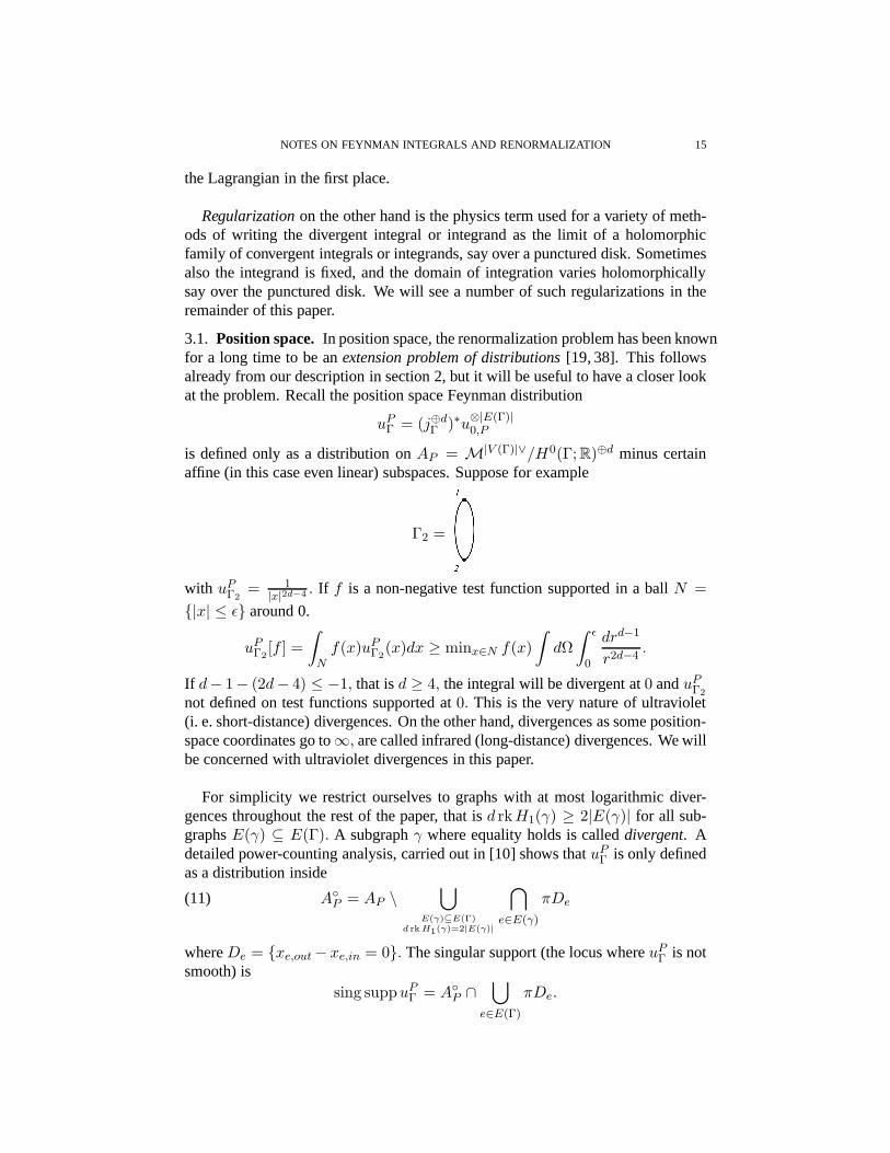
is defined only as a distribution onAP = M|V (Γ)|∨/H0(Γ;R)⊕d minus certainaffine (in this case even linear) subspaces. Suppose for example

Γ2 =

with uPΓ2= 1

|x|2d−4 . If f is a non-negative test function supported in a ballN =

|x| ≤ ǫ around 0.

uPΓ2[f ] =

∫

Nf(x)uPΓ2

(x)dx ≥ minx∈N f(x)

∫dΩ

∫ ǫ

0

drd−1

r2d−4.

If d− 1− (2d− 4) ≤ −1, that isd ≥ 4, the integral will be divergent at0 anduPΓ2

not defined on test functions supported at0. This is the very nature of ultraviolet(i. e. short-distance) divergences. On the other hand, divergences as some position-space coordinates go to∞, are called infrared (long-distance) divergences. We willbe concerned with ultraviolet divergences in this paper.

For simplicity we restrict ourselves to graphs with at most logarithmic diver-gences throughout the rest of the paper, that isd rkH1(γ) ≥ 2|E(γ)| for all sub-graphsE(γ) ⊆ E(Γ). A subgraphγ where equality holds is calleddivergent. Adetailed power-counting analysis, carried out in [10] shows thatuPΓ is only definedas a distribution inside

(11) AP = AP \

⋃

E(γ)⊆E(Γ)d rkH1(γ)=2|E(γ)|

⋂

e∈E(γ)

πDe

whereDe = xe,out− xe,in = 0. The singular support (the locus whereuPΓ is notsmooth) is

sing suppuPΓ = AP ∩

⋃

e∈E(Γ)

πDe.


An extension ofuPΓ fromAP toAP is called arenormalizationprovided it satisfies

certain consistency conditions to be discussed later.

In the traditional literature, which dates back to a centralpaper of Epstein andGlaser [38], an extension ofuPΓ from A

P to all of AP was obtained inductively,by starting with the case of two vertices, and embedding the solution (extension)for this case into the three, four, etc. vertex case using a partition of unity. Likethis, in each step only one extension onto a single point, say0, is necessary, a well-understood problem with a finite-dimensional degree of freedom: Two extensionsdiffer by a distribution supported at this point0, and the difference is therefore,by an elementary consideration, of the form

∑|α|≤n cα∂

αδ0 with cα ∈ C. Someof these parameterscα are fixed by physical requirements such as probability con-servation, Lorentz and gauge invariance, and more generally the requirement thatcertain differential equations be satisfied by the extendeddistributions. But evenafter these constants are fixed, there are degrees of freedomleft, and various groupsact on the space of possible extensions, which are collectively calledrenormaliza-tion group.For the at most logarithmic graphs considered in this paper,n = 0 andonly one constantc0 needs to be fixed in each step.

3.2. Resolution of singularities. The singularities, divergences and extensions(renormalizations) of the Feynman distributionuPΓ are best understood using a res-olution of singularities [10]. The Fulton-MacPherson compactification [43] intro-duced in a quantum field theory context by Kontsevich [49, 51]and Axelrod andSinger [6] serves as a universal smooth model where all position space Feynmandistributions can be renormalized. In [10], a graph-specific De Concini-ProcesiWonderful model [34] was used, in order to elaborate the striking match betweenDe Concini’s and Procesi’s notions of building set, nested set and notions found inQuantum Field Theory. No matter which smooth model is chosen, one disposesof a smooth manifoldY and a proper surjective map, in fact a composition ofblowups,

β : Y → AP

which is a diffeomorphism onβ−1(AP ) butβ−1(AP \A

P ) is (the real locus of) adivisor with normal crossings.

Instead of the nonorientable smooth manifoldY one can also find an orientablemanifold with cornersY ′ andβ a composition of real spherical blowups as in [6].In my pictures, the blowups are spherical because they are easier to draw, but inthe text they are projective.

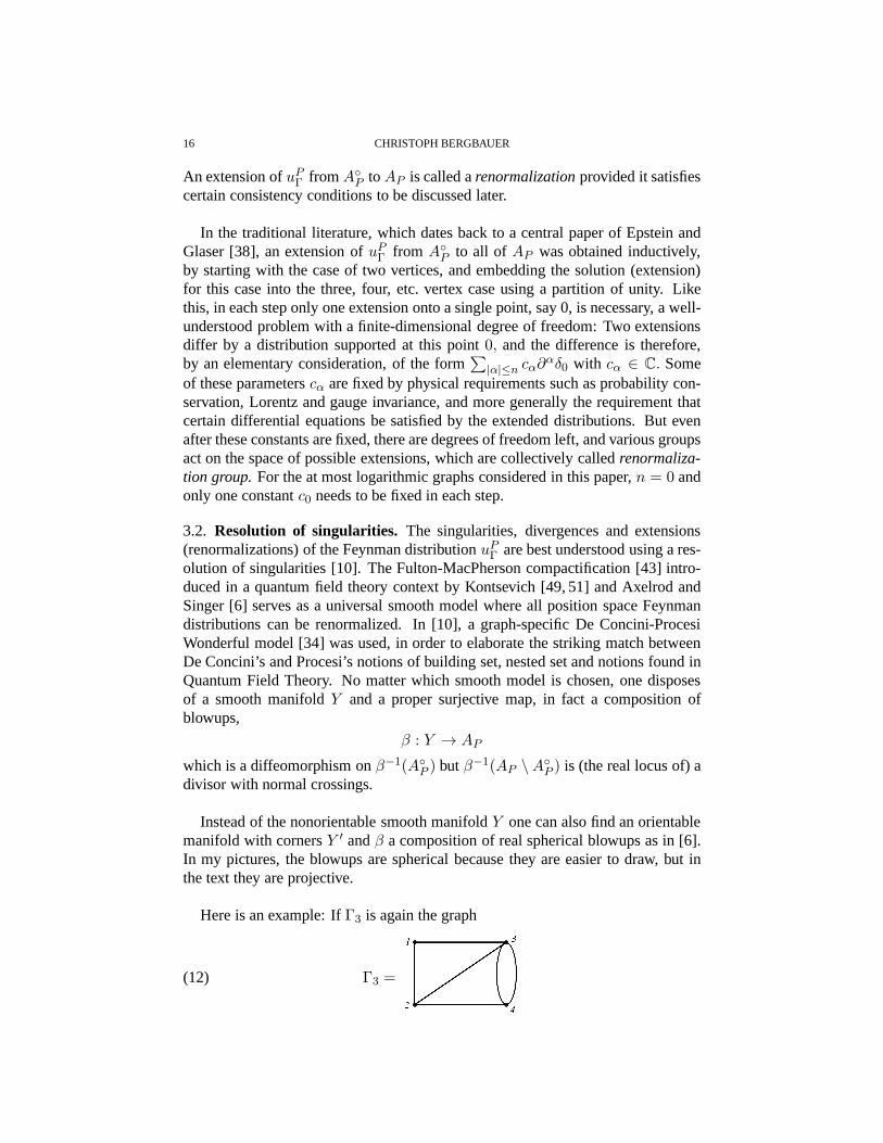
Here is an example: IfΓ3 is again the graph

(12) Γ3 =


andd = 4 then by (11) the locus where there are nonintegrable singularities is

D1234 ⊂ D234 ⊂ D34

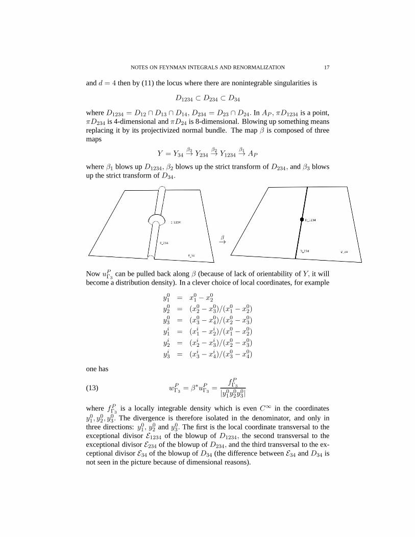
whereD1234 = D12 ∩D13 ∩D14, D234 = D23 ∩D24. In AP , πD1234 is a point,πD234 is 4-dimensional andπD24 is 8-dimensional. Blowing up something meansreplacing it by its projectivized normal bundle. The mapβ is composed of threemaps

Y = Y34β3→ Y234

β2→ Y1234

β1→ AP

whereβ1 blows upD1234, β2 blows up the strict transform ofD234, andβ3 blowsup the strict transform ofD34.

β→

Now uPΓ3can be pulled back alongβ (because of lack of orientability ofY, it will

become a distribution density). In a clever choice of local coordinates, for example

y01 = x01 − x02

y02 = (x02 − x03)/(x01 − x02)

y03 = (x03 − x04)/(x02 − x03)

yi1 = (xi1 − xi2)/(x01 − x02)

yi2 = (xi2 − xi3)/(x02 − x03)

yi3 = (xi3 − xi4)/(x03 − x04)

one has

(13) wPΓ3

= β∗uPΓ3=

fPΓ3

|y01y02y

03|

wherefPΓ3is a locally integrable density which is evenC∞ in the coordinates

y01, y02 , y

03. The divergence is therefore isolated in the denominator, and only in

three directions:y01 , y02 andy03. The first is the local coordinate transversal to the

exceptional divisorE1234 of the blowup ofD1234, the second transversal to theexceptional divisorE234 of the blowup ofD234, and the third transversal to the ex-ceptional divisorE34 of the blowup ofD34 (the difference betweenE34 andD34 isnot seen in the picture because of dimensional reasons).


For a general graphΓ, the total exceptional divisorE = β−1(AP \ AP ) has

normal crossings and the irreducible componentsEγ are indexed by connected di-vergent (consequently core) irreducible subgraphsγ. Moreover,

Eγ1 ∩ . . . ∩ Eγk 6= ∅ ⇐⇒ theγi are nested

where nested means each pair is either disjoint or one contained in the other. See[10] for the general result and more details.

Inspired by old papers of Atiyah [5], Bernstein and Gelfand [12] we used(uPΓ )s,

wheres in a complex number in a punctured neighborhood of 1, as a regularization[10]. Similarly, since the propagatoru0,P (x) = 1

|x|d−2 depends on the dimension,

one can also consideruPΓ with d in a punctured complex neighborhood of 4 as aregularization but I will not pursue this here.

Definition 3.1. A connected graphΓ is called primitive if

d rkH1(γ) = 2|E(γ)| ⇐⇒ E(γ) = E(Γ).

for all subgraphsE(γ) ⊆ E(Γ).

For a primitive graphΓp, only the single point0 ∈ AP needs to be blownup, and the pullback alongβ yields in suitable local coordinates (y01 = x01 − x02,

yji = (xji − xji+1)/(x01 − x02) otherwise)

β∗uPΓp=fΓp

|y01|

wherefΓp is a locally integrable distribution density constant iny01-direction. LetdΓ = d(|V (Γp)| − 1). Consequently

β∗(uPΓp)s =

f sΓp

|y01|dΓps−(dΓp−1)

It is well-known that the distribution-valued function1|x|s can be analytically in apunctured neighborhood ofs = 1, with a simple pole ats = 1. The residue of thispole isδ0 :

1

|x|s=

δ0s− 1

+|x|sfin, |x|sfin[f ] =

∫ 1

−1|x|s(f(x)−f(0))dx+

∫

R\[−1,1]|x|sf(x)dx.

This implies that the residue ats = 1 of β∗(uPΓp)s is a density supported at the

exceptional divisor (which is given in these coordinates byy0 = 0, and integratingthis density against the constant function1Y gives what is called the residue of thegraphΓp

resP Γp = ress=1 β∗(uPΓp

)s[1Y ] = −2

dΓp

∫

EfΓp

(The exceptional divisor can actually be oriented in such a way thatfΓp is a degree(dΓp − 1) differential form).


Let us now come back to the case ofΓ3 which is not primitive but has a nestedset of three divergent subgraphs. Raising (13) to a powers results in a pole ats = 1of order 3. The Laurent coefficienta−3 of (s− 1)−3 is supported on

E1234 ∩ E234 ∩ E34,

for this is the set given in local coordinates byy01 = y02 = y03 = 0. Similarly, thecoefficient of(s− 1)−2 is supported on

(E1234 ∩ E234) ∪ (E1234 ∩ E34) ∪ (E234 ∩ E34)

and the coefficient of(s− 1)−1 on

E1234 ∪ E234 ∪ E34.

(The non-negative part of the Laurent series is supported everywhere onY ). Write|dy| = |dy01 . . . dy

33|. In order to compute the coefficienta−3, one needs to integrate

fΓ3 , restricted to the subspacey01 = y02 = y03 = 0 :

fΓ3 =|dy|

(1 + y21)(1 + y2

2)(1 + y2

3)

×1

((1 + y02)2 + (y

1+ y02y2)

2)((1 + y03)2 + (y

2+ y03y3)

2))

whereyi

denotes the 3-vector(y1i , y2i , y

3i ). Consequently

fΓ3 |y01=y02=y03=0 =|dy|

(1 + y21)2(1 + y2

2)2(1 + y2

3)2

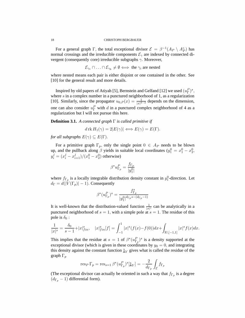
= f⊗3Γ1

whereΓ1 is the primitive graph with two vertices and two parallel edges joiningthem:

(14) Γ1 =

The chart where (13) holds covers actually everything ofYP up to a set of measurezero where there are no additional divergences. It suffices therefore to integrate inthese coordinates only. Several charts must be taken into account however whenthere are more than one maximal nested set. In conclusion,

(15) a−3[1Y ] = (resP Γ1)3,

a special case of a theorem in [10] relating pole coefficientsof β∗(uPΓ )s to residues

of graphs obtained fromΓ by contraction of divergent subgraphs.

But the ultimate reason to introduce the resolution of singularities in the firstplace is: In order to obtain an extension (renormalization)of uPΓ , one can now


simply remove the simple pole ats = 1 along each component of the exceptionaldivisor:

wPΓ3

=fΓ3

|y01y02y

03|,(16)

(wPΓ3)R =

fΓ3

|y01|fin|y02|fin|y

03|fin

.(17)

The second distribution(wPΓ3)R is defined on all ofY, and consequentlyβ∗(wP

Γ3)R

on all of AP . It agrees withuPΓ3on test functions having support inA

P and istherefore an extension. The difference betweenwP

Γ3and(wP

Γ3)R is a distribution

supported on the exceptional divisor which gives rise to a candidate for a countert-erm in the Lagrangian.

I call this renormalization schemelocal minimal subtraction, because locally,along each component of the exceptional divisor, the simplepole is removed in a”minimal way”, changing only the principal part of the Laurent series. See [10]for a proof that this results in local counterterms, a necessary condition for theextension to be a physically consistent one.

3.3. Momentum space. In momentum space, the bad definition of the positionspace Feynman distribution at certain diagonals

⋂De is translated by a Fourier

transform into ill-defined (divergent) integrals with divergences at certain strata atinfinity. For example, the position space integral(M, uPΓ1

= u20,P ) in d = 4 dimen-sions for the graphΓ1 (see (14)) has a divergence at0 (which is the imageπD12 ofthe diagonal). A formal Fourier transform would turn the pointwise productu20,Pinto a convolution product

(Fu20,P )(P ) =

∫u0,M(p)u0,M (p− P )d4p.

In fact the right hand side is exactlyUMΓ1(P )[1AΓ1

] in agreement with Proposi-tion 2.1. It does not converge at∞. (In order to see this we actually only needUMΓ1|P=0 = uMΓ1

, not the dependence upon external momenta).

On the other hand, the infrared singularities are to be foundat affine subspacesin momentum space. Of course the program sketched in the previous section canbe applied to the momentum space Feynman distribution as well: A resolution ofsingularities for the relevant strata at infinity can be found, and the pullback of themomentum space Feynman distribution can be extended onto all the irreduciblecomponents of the exceptional divisor. But I want to use thissection in order tosketch another, algebraic, approach to the momentum space renormalization prob-lem, which is due to Connes and Kreimer [29,30,53].

AssumeUMΓ [1AM

] varies holomorphically withd in a punctured disk aroundd = 4.Physicists call this dimensional regularization [32,39]:any integral

∫d4pu(p)dp

is replaced by ad-dimensional integral∫ddpu(p)dp. Like this we can consider


UMΓ as a distribution onall of AP×AM with values inR = C[[(d−4)−1, (d−4)]],

the field of Laurent series ind−4. If UMΓ [f ] is not convergent ind = 4 dimensions,

then there will be a pole atd = 4.

Let nowσΓ ∈ D′(AP ) be a distribution with compact support. Since the distri-butionUM

Γ is smooth in thePv, we can actually integrate it against the distributionσΓ (For example, ifσΓ = δ0(|Pv1 |

2−E1)⊗ . . .⊗δ0(|P2vn |−En) then this amounts

simply to evaluatingUMΓ at the subspaces|Pv1 |

2 = E1, . . . , |Pv2 |2 = En). In any

case we have a map

φ : (Γ, σΓ) 7→ UMΓ [1AM

⊗ σΓ] ∈ R

sending pairs to Laurent series. Let nowH be the polynomial algebra overCgenerated by isomorphism classes of connected core divergent graphsΓ of a givenrenormalizable quantum field theory. Define a coproduct∆ by

∆(Γ) = 1⊗ Γ + Γ⊗ 1 +∑

γ1⊔...⊔γk(Γconn. core div.

γ1 · · · γk ⊗ Γ//(γ1 ⊔ . . . ⊔ γk).

The notationΓ//γ means that any connected component ofγ insideΓ is contractedto a (separate) vertex. By standard constructions [29],H becomes a Hopf algebra,called Connes-Kreimer Hopf algebra. Denote the antipode byS. Let nowHσ bethe corresponding Hopf algebra of pairs(Γ, σΓ) (In order to define this Hopf alge-bra of pairs, one needs the extra condition thatσΓ vanishes on all vertices that haveno external edges, a standard assumption if one considers only graphs of a fixedrenormalizable theory).

The mapφ : Hσ → R is a homomorphism of unitalC-algebras. The space ofthese mapsHσ → R is a group with the convolution productφ1 ⋆ φ2 = m(φ1 ⊗φ2)∆. OnR, there is the linear projection

(18) R : (d− 4)n 7→

0 if n ≥ 0(d− 4)n if n < 0

onto the principal part.

Theorem 3.1(Connes, Kreimer). The renormalized Feynman integralφR(Γ, σΓ)|d=4

and the countertermSφR(Γ, σΓ) are given as follows. I denoteΓ for the pair

(Γ, σΓ) :

SφR(Γ) = −R

φ(Γ) +

∑

γ=γ1⊔...⊔γk(Γconn. core div.

SφR(γ)φ(Γ//γ)

φR(Γ) = (1−R)

φ(Γ) +

∑

γ=γ1⊔...⊔γk(Γconn. core div.

SφR(γ)φ(Γ//γ)


These expressions are assembled from the formula for the antipode and the con-volution product. Combinatorially, the Hopf algebra encodes the BPHZ recursion[46] and Zimmermann’s forest formula [89]. The theorem can be interpreted as aBirkhoff decomposition of the characterφ into φ− = Sφ

R andφ+ = φR [30].

The renormalization scheme described here is what I callglobal minimal sub-traction, because in the target fieldR, when all local information has been inte-grated out, the map1 − R removes only the entire principal part atd = 4. Thiscoincides with the renormalization scheme described in [28].

In the case ofm = 0 and zero-momentum transfer (all but two external momentaset to 0) one knows that atd = 4

(19) φR(Γ) =

N∑

n=0

pn(Γ)(log |P |2/µ2)n, pn(Γ) ∈ R

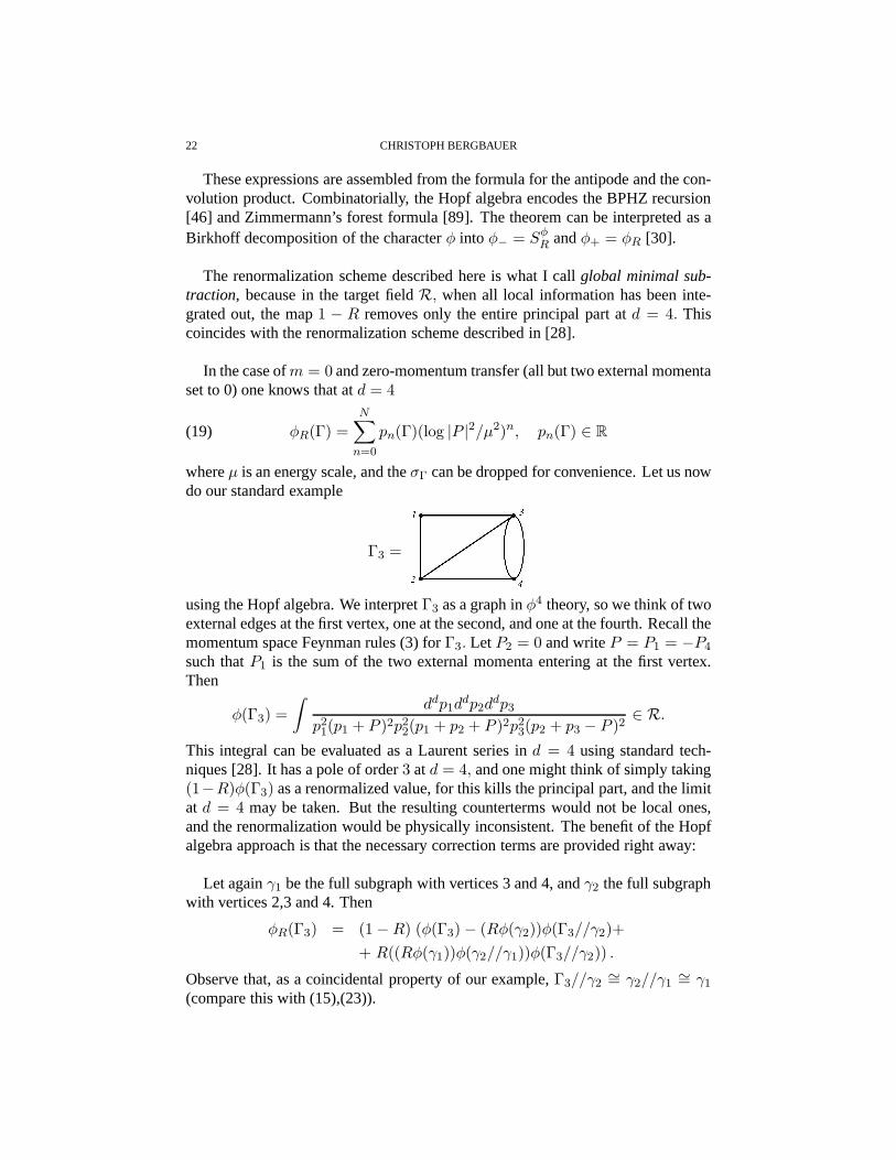
whereµ is an energy scale, and theσΓ can be dropped for convenience. Let us nowdo our standard example

Γ3 =

using the Hopf algebra. We interpretΓ3 as a graph inφ4 theory, so we think of twoexternal edges at the first vertex, one at the second, and one at the fourth. Recall themomentum space Feynman rules (3) forΓ3. LetP2 = 0 and writeP = P1 = −P4

such thatP1 is the sum of the two external momenta entering at the first vertex.Then

φ(Γ3) =

∫ddp1d

dp2ddp3

p21(p1 + P )2p22(p1 + p2 + P )2p23(p2 + p3 − P )2∈ R.

This integral can be evaluated as a Laurent series ind = 4 using standard tech-niques [28]. It has a pole of order3 atd = 4, and one might think of simply taking(1−R)φ(Γ3) as a renormalized value, for this kills the principal part, and the limitat d = 4 may be taken. But the resulting counterterms would not be local ones,and the renormalization would be physically inconsistent.The benefit of the Hopfalgebra approach is that the necessary correction terms areprovided right away:

Let againγ1 be the full subgraph with vertices 3 and 4, andγ2 the full subgraphwith vertices 2,3 and 4. Then

φR(Γ3) = (1−R) (φ(Γ3)− (Rφ(γ2))φ(Γ3//γ2)+

+ R((Rφ(γ1))φ(γ2//γ1))φ(Γ3//γ2)) .

Observe that, as a coincidental property of our example,Γ3//γ2 ∼= γ2//γ1 ∼= γ1(compare this with (15),(23)).


The Hopf algebra approach to renormalization has brought upa number of sur-prising connections to other fields, see for example [30,31,37,41,59,64,67,79,80].Other developments starting from the Connes-Kreimer theory can be found in [32].Kreimer and van Suijlekom have shown that gauge and other symmetries are com-patible with the Hopf algebra structure [55,61,78,84,85].

A sketch how the combinatorics of the Hopf algebra relate to the resolution ofsingularities in the previous section and to position spacerenormalization can befound in [10], see also section 3.6.

3.4. Parametric representation. In the parametric representation introduced insection 2.2, the divergences can be found at certain intersections of the coordinatehyperplanesAe = ae = 0. This is in fact one of the very reasons why the para-metric representation was introduced: Consider for example the divergent integral(R4, u20,M ), with u0,M = 1

|p|2,

∫d4p

|p|4=

∫ ∫ ∞

0

∫ ∞

0exp(−a1|p|

2 − a2|p|2)da1da2d

4p

in the sense of Definition 2.1 (In this section, instead of(A, u) I will simply write∫A u(x)dx.) The integral at the left hand side is divergent both at0 and at∞. But

splitting it into the two parts at the right, and interchanging thed4pwith theda1da2integrations leaves a gaussian integral

∫exp(−

c

2|p|2)ddp = (2π/c)d/2

which is convergent, but at the expense of getting(a1 + a2)2 in the denominator:

The integral ∫ ∞

0

∫ ∞

0

da1da2(a1 + a2)2

has a logarithmic singularity at0 and at∞. This can be seen by blowing up theorigin inR2

≥0, and pulling back:∫ ∞

0

∫ ∞

0

db1db2b1(1 + b2)2

.

In other words, the trick with the parametric parameterization (calledSchwingertrick in [15]), does not get rid of any divergences. It just moves them into another,lower-dimensional space.

Again it is useful to have a resolution of singularities in order to separate thevarious singularities and divergences of a graph along irreducible components ofa divisor with normal crossings. The most obvious and efficient such resolution isgiven in [15,16]:

Let Γ be core. For a subgraphE(γ) ⊆ E(Γ), let

Lγ = ∩e∈E(γ)Ae = ae = 0, e ∈ E(γ),


a linear subspace. SetLcore = Lγ : γ is a core subgraph ofΓ, and

L0 = minimal element ofLcore = 0

Ln+1 = minimal elements ofLcore \n⊔

i=0

Li

This partition ofLcore is made in such a way that (see [16, Proposition 3.1]) asequence of blowups

(20) γ : ZS → . . .→ AS

is possible which starts by blowing upL0 and then successively the strict trans-forms of the elements ofL1,L2, . . . This ends up withZS a manifold with corners.The mapγ is of course defined not only as a map ontoAS = R

|E(Γ)|≥0 but as a

birational mapγ : ZS → C|E(Γ)|, with ZS a smooth complex variety. The to-tal exceptional divisorE has normal crossings, and one componentEL for eachL ∈ Lcore. (In the language of section 3.2,Lcore is the building set). Moreover,

EL1 ∩ . . . ∩ ELk6= 0 ⇐⇒ theLi are totally ordered by inclusion.

Since the coordinate divisorae = 0 for somee ∈ E(Γ) has already normalcrossings by definition, the purpose of these blowups is really only to pull out intocodimension 1 all the intersections where there are possibly singularities or diver-gences, and to separate the integrable singularities of theintegrand from this set asmuch as possible.

Note that in the parametric situation where the domain of integration is the man-ifold with cornersR|E(Γ)|

≥0 , the blowups do not introduce an orientation issue on thereal locus.

For the example graphΓ3 of the previous sections (see (12)),

uSΓ3=

da1 . . . da6

((a1 + a2)((a3 + a4)(a5 + a6) + a5a6) + a3a4a5 + a3a4a6 + a3a5a6)d/2

we examine the pullback ofuSΓ3onto ZS . There are various core subgraphs to

consider, but it is easily seen, in complete analogy with (11), that the divergencesare located only atLΓ3 , Lγ2 andLγ1 whereγ1 is the full subgraph with vertices3 and 4, andγ2 the full subgraph with vertices 2,3 and 4. In order to see thedivergences inZS , it therefore suffices to look in a chart whereELΓ3

, ELγ2andELγ1

intersect. In such a chart, given by coordinatesb1 = a1, b2 = a2/a1, b3 = a3/a1,b4 = a4/a1, b5 = a5/a3, b6 = a6/a5, we have(21)

γ∗uSΓ3=

db1 . . . db6

b1b3b5((1 + b2)((1 + b6)(1 + b4) + b5b6) + b3(b5b6 + b4b6 + b4))d/2

Now we are in a very similar position as in the previous section. If Γp is a primitivegraph, then there is only the origin0 ∈ AS which needs to be blown up in orderto isolate the divergence. SinceuSΓ3

depends explicitly ond in the exponent, let us


used as an analytic regulator. One finds, using for example coordinatesb1 = a1,bi = ai/a1, i 6= 1, in a neighborhood ofd = 4,

γ∗uSΓp(d) =

(δ0(b1)

d− 4+ finite

)gΓp

with gΓp ∈ L1loc. (If one wants even a regulargΓp one needs to perform the remain-

ing blowups in (20).) Then we define

(22) resS Γp = (resd=4 γ∗uSΓp

(d))[1] =

∫

b1=0,bi≥0gΓp =

∫

σ

Ω

Ψ2Γp

whereσ = ai ≥ 0 ⊂ P|E(Γ)|−1(R) andΩ =∑|E(Γ)|

n=1 (−1)nanda1 ∧ . . .∧ dan ∧. . . ∧ da|E(Γ)|. The last integral at the right is a projective integral, meaning that

theai are interpreted as homogeneous coordinates ofP|E(Γ)|−1. By choosing affinecoordinatesbi, one finds that it is identical with the integral ofgΓp over the excep-tional divisor intersected with the total inverse image ofAS .

Coming back to the non-primitive graphΓ3 (see (21)) we find in complete analogywith section 3.2, that

uSΓ3(d) =

∞∑

n≥−3

cn(d− 4)n

in a neighborhood ofd = 4, and

(23) c−3[1AS] = (resS Γ1)

3

which is easily seen by sendingb1, b3, b5 to 0 in (21):gΓ3 |b1=b3=b5=0 = g⊗3Γ1.

Similarly, one can translate the results of section 3.2 and [10] into this setting andobtain a renormalization (extension ofuSΓ) by removing the simple pole along eachcomponent of the irreducible divisor. In section 4.5 a different, motivic renormal-ization scheme for the parametric representation will be studied, following [16].

3.5. Dyson-Schwinger equations.Up to now we have only considered singleFeynman graphs, with internal edges interpreted as virtualparticles, and param-eters such as the mass subjected to renormalization. Another approach is to startwith the full physical particles from the beginning, that is, with the non-perturbativeobjects. Implicit equations satisfied by the physical particles (full propagators) andthe physical interactions (full vertices) are calledDyson-Schwinger equations.Theequations can be imposed in a Hopf algebra of Feynman graphs [11,23,57,58,88]and turn into systems of integral equations when Feynman rules are applied.

For general configurations of external momenta, Dyson-Schwinger equationsare extremely hard to solve. But if one sets all but two external momenta to 0,a situation called zero-momentum transfer (see (19)), thenthe problem simplifiesconsiderably.


In [60], an example of a linear Dyson-Schwinger equation is given which canbe solved nonperturbatively by a very simple Ansatz. More difficult non-linearDyson-Schwinger equations, and finally systems of Dyson-Schwinger equationsas above, are studied in [62,63,82,83], see also [40,56,88].

3.6. Remarks on minimal subtraction. I come back at this point to the differencebetween what I calllocal (section 3.2) andglobal (section 3.3)minimal subtrac-tion, which, I think, is an important one.

I tried to emphasize in the exposition of the previous sections that the key con-cepts of renormalization are largely independent of whether momentum space, po-sition space, or parametric space Feynman rules are used. This is immediately seenin the Connes-Kreimer Hopf algebra framework where a graphΓ and some exter-nal informationσΓ are sent directly to a Laurent series ind− 4. For this we don’tget to see and don’t need to know if the integral has been computed in momentum,position, or parametric space. They all produce the same number (or rather Laurentseries), provided the same regularization is chosen for allthree of them.

In position space, where people traditionally like to work with distributions aslong as possible and integrate them against a test function only at the very end (oreven against the constant function1, the adiabatic limit), one is tempted to definethe Feynman rules as a map into a space of distribution-valued Laurent series, as wehave done it in [10]. But one has to be aware that this space of distribution-valuedLaurent series does not necessarily qualify as a replacement for the ringR in sec-tion 3.3 if one looks for a new Birkhoff decomposition. In general, many questionsand misconceptions that I have encountered in this area can be traced back to thedecision at which moment one integrates, and minimal subtraction seems to be agood example for this.

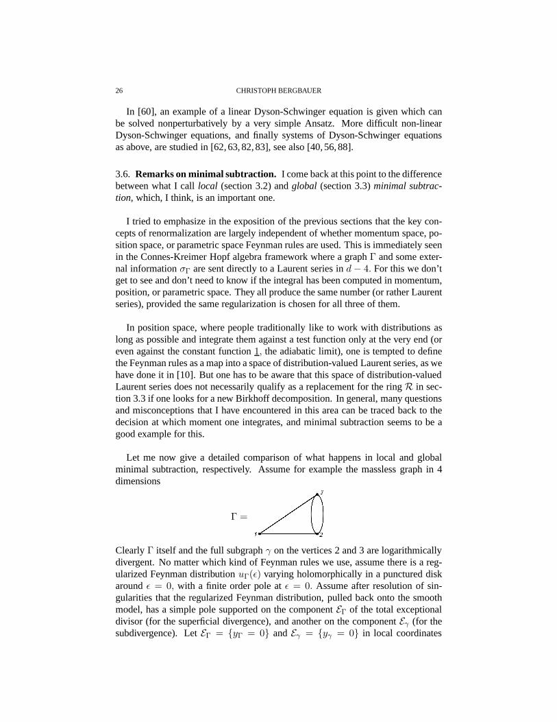
Let me now give a detailed comparison of what happens in localand globalminimal subtraction, respectively. Assume for example themassless graph in 4dimensions

Γ =

ClearlyΓ itself and the full subgraphγ on the vertices 2 and 3 are logarithmicallydivergent. No matter which kind of Feynman rules we use, assume there is a reg-ularized Feynman distributionuΓ(ǫ) varying holomorphically in a punctured diskaroundǫ = 0, with a finite order pole atǫ = 0. Assume after resolution of sin-gularities that the regularized Feynman distribution, pulled back onto the smoothmodel, has a simple pole supported on the componentEΓ of the total exceptionaldivisor (for the superficial divergence), and another on thecomponentEγ (for thesubdivergence). LetEΓ = yΓ = 0 andEγ = yγ = 0 in local coordinates


yΓ, yγ , y3, . . . , yn.

(24) uΓ(ǫ) =

(δ0(yΓ)

ǫ+ |yΓ|fin(ǫ)

)(δ0(yγ)

ǫ+ |yγ |fin(ǫ)

)fΓ(ǫ)

wherefΓ is locally integrable and smooth inyΓ and yγ , such that in particularfΓ(ǫ) is holomorphic inǫ. There is accordingly a second order pole supported atEΓ ∩ Eγ . We know from [10], as was also sketched in section 3.2, that the leadingcoefficient of this second order pole is a product of delta functions restricting it toEΓ ∩ Eγ times the residue ofγ times the residue ofΓ//γ.

Consequently, integratinguΓ(ǫ) against a fixed functionχ (for a first readingtakeχ = 1 but in the massless case, one has to worry about infared divergences)provides a Laurent series

uΓ(ǫ)[χ] = a−2ǫ−2 + a−1ǫ

−1 + a0ǫ0 + . . .

Sinceγ andΓ//γ are primitive,

uγ(ǫ)[χ] = b−1ǫ−1 + b0ǫ

0 + b1ǫ1 + . . .

uΓ//γ(ǫ)[χ] = c−1ǫ−1 + c0ǫ

0 + b1ǫ1 + . . .

We know from the previous remarks thata−2 = res(γ) res(Γ//γ) = b−1c−1 andsimilarly a−1 = b−1c0 + g where I don’t want to specifyg.

Let me now compare local and global minimal subtraction at this example. Lo-cal minimal subtraction is defined on distribution-valued Laurent series, but globalminimal subtraction only onC-valued Laurent series. Therefore we need to in-tegrate everything out before comparing. I start with localminimal subtraction(LMS). In order to get from (24) to

(25) (uΓ)R,LMS(ǫ) = |yΓ|fin(ǫ)|yγ |fin(ǫ)fΓ(ǫ)

one has to subtract three terms from (24):

RΓLMSuΓ(ǫ) =

δ0(yΓ)

ǫ

(δ0(yγ)

ǫ+ |yγ |fin(ǫ)

)fΓ(ǫ)

Rγ,Γ//γLMS uΓ(ǫ) =

(δ0(yΓ)

ǫ+ |yΓ|fin(ǫ)

)δ0(yγ)

ǫfΓ(ǫ)

−RRγ,Γ//γLMS uΓ(ǫ) = −

δ0(yΓ)

ǫ

δ0(yγ)

ǫfΓ(ǫ)

The first term cleans the pole supported onEΓ, such thatuΓ −RΓLMSuΓ has only a

simple pole supported onEγ left. On the other hand,uΓ − Rγ,Γ//γLMS uΓ has only a

simple pole supported onEΓ left, and the third term is a correction term supportedonEγ ∩ EΓ accounting for what has been subtracted twice. In summary,

(26) (uΓ)R,LMS(ǫ) = uΓ(ǫ)−RΓLMSuΓ(ǫ)−R

γ,Γ//γLMS uΓ(ǫ) +RR

γ,Γ//γLMS uΓ(ǫ)

is the result of local minimal subtraction.


Let us now integrate out (26).

uΓ(ǫ)[χ] = a−2ǫ−2 + a−1ǫ

−1 + a0ǫ0 + . . .

RΓLMSuΓ(ǫ)[χ] = a−2ǫ

−2 + gǫ−1 + hǫ0 + . . .

Rγ,Γ//γLMS uΓ(ǫ)[χ] = a−2ǫ

−2 + b−1c0ǫ−1 + b−1c1ǫ

0 + . . .

−RRγ,Γ//γLMS uΓ(ǫ)[χ] = a−2ǫ

−2

These equations follow from (24), and I don’t want to specifyh. Consequently

(uΓ)R,LMS(ǫ)[χ] = a0 − b−1c1 − h asǫ → 0.

In global minimal subtraction (GMS), whereRGMS = R as in (18), somethingdifferent happens.

RGMS(uΓ(ǫ)[χ]) = a−2ǫ−2 + a−1ǫ

−1

(RGMSuγ(ǫ)[χ])uΓ//γ (ǫ)[χ] = b−1c−1ǫ−2 + b−1c0ǫ

−1 + b−1c1ǫ0 + . . .

−RGMS(RGMSuγ(ǫ)[χ])uΓ//γ(ǫ)[χ]) = b−1c−1ǫ−2 + b−1c0ǫ

−1

The first subtractionuΓ[χ]−RGMS(uΓ[χ]) removes the poles everywhere, also theone supported onEγ which has nothing to do with the superficial divergence. Thethird and fourth term restore the locality of counterterms.We have

(uΓ)R,GMS(ǫ)[χ] = a0 − b−1c1 asǫ→ 0.

In summary: Unlessh = 0, local and global minimal subtraction differ by a fi-nite renormalization. Moreover, although there is a one-to-one-correspondencebetween terms to be subtracted in LMS and GMS, the values of those single termsdo not agree. It seems to me that GMS is a quite clever but somehow exceptionaltrick of defining the subtraction operatorR onC-valued Laurent series where allthe geometric information (i. e. where the pole is supported) has been forgotten.

In [10] it is shown how to relate, for a general graphΓ, the combinatorics of thetotal exceptional divisor of the resolution of singularities to the Connes-KreimerHopf algebra of Feynman graphs, such that the example presented here is a specialcase of a more general result. A similar analysis applies to other local renormal-ization prescriptions, called subtraction at fixed conditions in [10], as well.

4. MOTIVES AND RESIDUES OFFEYNMAN GRAPHS

4.1. Motives, Hodge Realization and Periods.Much of the present interest inFeynman integrals is due to the more or less obvious fact thatthere is somethingmotivicabout them. In order to understand and appreciate this, one obviously needsto have an idea of what a motive is. I am not an expert in this area and will noteven attempt to provide much background to the notion of motive. See [4] for anoften cited introduction to the subject, which I follow closely in the beginning ofthis section.


The theory of motives is a means to unify the various cohomology theoriesknown for algebraic varietiesX over a number fieldk. Such cohomology theo-ries include the algebraic de Rham and the Betti cohomology,but there are manyothers. The algebraic de Rham cohomologyH•

dR(X) is defined over the groundfield k, and Betti cohomologyH•

B(X;Q) is the singular cohomology ofX(C)with rational coefficients.

A motive of a variety is supposed to be a piece of a universal cohomology, suchthat all the usual cohomology theories (functors from varieties to graded vectorspaces) factor through the category of motives. A particular cohomology theoryis then called arealization. For example, the combination of de Rham and Betticohomology, giving rise to a Hodge structure, is calledHodge realization.

The theory of motives is not complete yet. Only for the simplest kind of alge-braic varieties, smooth projective ones, a category of motives with the desired prop-erties has been constructed. These motives are calledpure. For general, i. e. sin-gular or non-projective varieties, the theory is conjectural in the sense that onlya triangulated category as a candidate for the derived category of the category ofthese motives, calledmixed motivesexists.

LetX be a smooth variety overQ. LetH•dR(X) denote the algebraic de Rham

cohomology ofX, a gradedQ-vector space, andH•B(X;Q) the rational Betti coho-

mology (singular cohomology of the complex manifoldX(C) with rational coeffi-cients), a gradedQ-vector space. Aperiod of X is by definition a matrix elementof thecomparison isomorphism(integration)

H•dR(X)⊗Q C ∼= H•

B(X;Q)⊗Q C

for a suitable choice of basis. A period is therefore in particular an integral of analgebraic differential form over a topological cycle onX(C). A standard exampleis the case of an elliptic curveX defined by the equationy2 = x(x − 1)(x − λ),λ ∈ Q \ 0, 1. A basis element ofH1

dR(X) is the 1-formω = dx2y and and a basis

of the singular cohomologyH1B(X) is given by the duals of two circles around the

cut between0 and1 resp. the cut between1 and∞. Integratingω against thesecycles gives the generators of the period lattice ofX.

Similarly, matrix elements of a comparison isomorphism betweenrelative co-homologies of pairs(X,A) are calledrelative periods. Many examples consideredbelow will be relative periods.

4.2. Multiple zeta values, mixed Tate motives and the work of Belkale andBrosnan. Let Γ be a primitive Feynman graph. I assumed = 4 andm = 0.Recall the graph polynomial

ΨΓ =∑

T st of Γ

∏

e 6∈E(T )

ae ∈ Z[ae : e ∈ E(Γ)]


from (5). The sum is over the spanning trees ofΓ. Following [15], we have a closerlook at the parametric residue

resS Γ =

∫

σ

Ω

Ψ2Γ

introduced in (22). LetXΓ = ΨΓ = 0 ⊂ P|E(Γ)|−1 andCXΓ = ΨΓ =

0 ⊂ A|E(Γ)| its affine cone.XΓ resp.CXΓ are calledprojectiveresp.affine graphhypersurface. The chain of integration isσ = ae ≥ 0 ⊆ P|E(Γ)|−1(R), andΩ =

∑(−1)nanda1 ∧ . . . ∧ dan ∧ . . . ∧ da|E(Γ)|.

The residueresS Γ already looks like a relative period, sinceσ has its boundarycontained in the coordinate divisor∆ =

⋃e∈E(Γ)ae = 0, and the differential

form ΩΨ2

Γis algebraic (i. e. regular) inP|E(Γ)|−1 \ XΓ. But in generalXΓ ∩ ∆ is

quite big, andΩΨ2

Γ6∈ H

|E(Γ)|−1dR (P|E(Γ)|−1 \XΓ,∆ \ (XΓ ∩∆)).

The solution is of course to work in the blowupZS of section 3.4 where thingsare separated. LetPS be the variety obtained fromP|E(Γ)|−1 by regarding all ele-ments of theLn (n ≥ 1) in section 3.4 as subspaces ofP|E(Γ)|−1 and starting theblowup sequence atn = 1 instead ofn = 0.

In [15,16] it is shown thatPS has the desired properties: the strict transform ofXΓ does not meet the strict transform ofσ. Like this, resS Γ is a relative period ofthe pair

(PS \ YΓ, B \ (B ∩ YΓ))

whereYΓ is the strict transform ofXΓ, andB the total transform of the coordinatedivisor∆.

We callresS Γ aFeynman periodof Γ.

An empirical observation due to Broadhurst and Kreimer [21,22] was that allFeynman periods computed so far are rational linear combinations of multiple zetavalues.

A multiple zeta valueof depthk and weights = s1 + . . . + sk is a real numberdefined as follows:

ζ(s1, . . . , sk) =∑

1≤nk<...<n1

1

ns11 . . . nskk

wheres1 ≥ 2 ands2, . . . , sk ≥ 1. Fork = 1 one obtains the values of the Riemannzeta function at integer arguments≥ 2, whence the name.


By an observation due to Euler and Kontsevich, multiple zetavalues can bewritten as iterated integrals

ζ(s1, . . . , sk) =

∫

0<ts<...<t1<1ws1 ∧ . . . ∧ wsk

where

ws(t) =

(dt

t

)∧(s−1)

∧dt

1− t

and therefore qualify already asnaive periods, as defined in [52].

But in order to understand multiple zeta values as (relative) periods of the coho-mology of something, one needs to go one step further and introduce the modulispaceM0,s+3 of genus0 curves withs+3 distinct marked points, and its Deligne-Mumford compactificationM0,s+3.

Indeed, starting from the iterated integral representation, ζ(s1, . . . , sk) can beshown to be a relative period of a pair

(M0,s+3 \ A,B \ (A ∩B))

with A andB suitable divisors which have no common irreducible component.These pairs havemixed Tatemotives, a special (and relatively simple and well-understood) kind of mixed motives. This is a result of Goncharov and Manin [44].Brown showed that conversely every such relative period ofM0,s+3 is a rationallinear combination of multiple zeta values [26].

Let us now come back to the Feynman periods. Even up to now, nota single ex-ample of a Feynman period is known which is not a rational linear combination ofmultiple zeta values. Moreover, these multiple zeta valuesdo not arise randomly,but there are already certain patterns visible. For examples of such patterns, see[15,21,22,76].

Motivated by an (informal) conjecture of Kontsevich [50], Belkale and Brosnaninvestigated the motives associated to Feynman graph hypersurfaces. Kontsevich’sconjecture did not state directly that all Feynman periods be multiple zeta values,but that the function

q 7→ |CXΓ(Fq)|

be a polynomial inq for all Γ. Using another conjecture about motives, a non-polynomial counting function for the number of points ofCXΓ over Fq wouldimply thatCXΓ has a period which isnot in theQ-span of multiple zeta values.For example, an elliptic curve is known to have a non-polynomial point countingfunction.

Belkale and Brosnan came to the surprising result that Kontsevich’s conjectureis false [7], and that Feynman graph hypersurfaces have the most general motivesone can think of.


4.3. Matroids and Mn ev’s theorem. One key idea in Belkale’s and Brosnan’sproof was to study more general schemes defined by matroids:

Definition 4.1. LetE be a finite set andI ⊆ 2E . The pairM = (E, I) is calledmatroidif

(1) ∅ ∈ I,(2) A1 ⊆ A2, A2 ∈ I =⇒ A1 ∈ I,(3) A1, A2 ∈ I, |A2| > |A1| =⇒ there is anx ∈ A2 \ A2 ∩ A1 such that

A1 ∪ x ∈ I.

The numberrkM = maxA∈I |A| is calledrank ofM.

The subsetsA ∈ I where|A| is maximal are calledbasesof M. The literatureusually names two standard examples for matroids:

(1) M = (E, I) whereE is a finite set of vectors in somekr, I the set oflinearly independent subsets ofE. ClearlyrkM ≤ r.

(2) M = (E, I) whereE is the set of edges of a graph andI the set of sub-graphs (each determined by a subset of edges) without cycles. ClearlyrkM = |V (Γ)| − rkH0(Γ;Z).

We have already seen in section 2.1 how these examples are related (in fact, thesecond is a special case of the first): IfΓ is a graph, for eache ∈ E(Γ) there is alinear forme∨jΓ onR|V (Γ)|/H0(Γ;R), and such linear formse∨1 jΓ, . . . , e

∨njΓ are

pairwise linearly independent if and only if the graph with edgese1, . . . , en hasno cycles.

Let us return to the general case. A matroid is equivalently characterized by arank function on2E as follows:

Definition 4.2. A mapr : 2E → N is calledrank functionif

(1) r(A) ≤ |A|,(2) A1 ⊆ A2 =⇒ r(A1) ≤ r(A2),(3) r(A1 ∪A2) + r(A1 ∩A2) ≤ r(A1) + r(A2).

Proposition 4.1. LetM = (E, I) be a matroid. Then the map

r : A 7→ rk(A, B ∈ I,B ⊆ A)

is a rank function. Conversely, letE be a finite set andr a rank function for it.ThenM = (E, r) = (E, I) whereI = A ⊆ E, r(A) = |A| is a matroid.

We have seen how linearly independent subsets of vectors in avector space giverise to a matroid. On the other hand one may ask if every matroid is obtained thisway:

Definition 4.3. Letk be a field. A matroidM = (E, r) is calledrealizable overkis there is anr ∈ N and a mapf : E → kr with dim span f(A) = r(A) for allA ∈ 2E . Such a map is calledrepresentation ofM .


There are matroids which are representable only over certain fields, for examplethe Fano matroid.

The spaceX(M,s) of all representations ofM in ks (a subvariety ofAs|E| de-fined overk) is calledrepresentation spaceof M. It is a fundamental question howgeneral these realization spaces are. An answer is given by Mnev’s UniversalityTheorem.

Mnev’s Universality Theorem was originally proved by Mnev in a context oforiented matroidsand their representations over the ordered field of real numbers.Without giving a precise definition, an oriented matroid keeps not only track ofwhether or not certain subsets of vectors are linearly dependent but also about thesign of determinants: Roughly an oriented matroid is specified by a list of partitionsof E indicating which vectors inE may be separated by linear hyperplanes inRn. Again the representation space of an oriented matroid is thespace of vectorconfigurations which leaves this list of partitions invariant. The original, quitedifficult, version of the theorem is then

Theorem 4.1(Mnev, oriented version). For every primary semi-algebraic setXin Rr defined overZ there is an oriented matroid whose realization space is stablyequivalent toX.

Here a primary semi-algebraic set defined overZ is a set given by polynomialequations andsharppolynomial inequalities<,> with integer coefficients, (suchasx21 + x22 > 2, x2x

31 = 1), and stable equivalence means roughly a sort of ho-

motopy equivalence preserving certain arithmetic properties. The proof in Mnev’sthesis [68, 69] is quite intricate, and there is a simplified proof in [7, 73] which Ifollow here.

The simpler version that we need is obtained by replacing primary semi-algebraicsets by affine schemes of finite type overSpecZ, oriented matroids by matroids,and stable equivalent by isomorphic with an open subscheme in a product withAN .Just like the affine representation space, there is a projective representation space

X(M,s) = f : E → Ps−1 :

dim span f(A) = r(A)− 1 for all A ∈ 2E

Theorem 4.2 (Mnev, un-oriented version). Let X be an affine scheme of finitetype overSpecZ. Then there is a matroidM of rank 3,N ∈ N and an openU ⊆ X × AN projecting surjectively ontoX such that

U ∼= X(M, 3)/PGL3.

This is the version in Lafforgue’s book [65]. I am grateful toA. Usnich forshowing me this reference. See also [20] for the independently obtained version ofSturmfels.


SupposeX is defined byf+ − f− = 0 wheref+ andf− are polynomials withpositive coefficients. Thef± can be successively decomposed into more elemen-tary expressions involving only one addition or one multiplication at a time, at theexpense of introducing many more variables. The proof of Theorem 4.2 uses thenthe fact that oncex1 andx2 are fixed on a projective line,x1+x2 andx1x2 etc. canbe determined by linear dependence conditions in the projective plane (this is whythe rank ofM is only 3). The difficulties left are to relate different projective scalesand to avoid unwanted dependencies.

Like this any affine scheme overSpecZ is related to the representation space ofa (huge) rank 3 matroid. Belkale and Brosnan use a slightly different version ofMnev’s theorem and then show (a lot of work that I just skip) how this representa-tion space is connected to the graph hypersurfacesCXΓ.

Let me now state the main result of [7]: LetGeoMot+ be the abelian group withgenerators isomorphism classes[X] of schemesX of finite type overZ modulo therelation

[X] = [X \ V ] + [V ]

if V is a closed subscheme ofX. Endowed with the cartesian product[X][Y ] =[X × Y ], GeoMot+ becomes a ring with unit[SpecZ]. Let L = [A1] be the Tatemotive, andS the saturated multiplicative subset ofZ[L] generated byLn − L forn > 1. Let GeoMot = S−1GeoMot+, andGraphs theS−1Z[L]-submodule ofGeoMot generated by the[CXΓ], whereΓ are Feynman graphs.

Theorem 4.3(Belkale, Brosnan). Graphs = GeoMot .

It is clear that point-countingq 7→ |X(Fq)| factors throughGeoMot . ThereforeKontsevich’s conjecture is false. Also it is known [7, Section 15] that the mixedTate property can be detected inGeoMot . Therefore it follows that not allXΓ aremixed Tate, and (using another conjecture) that not all periods of allXΓ are ratio-nal linear combinations of multiple zeta values.

On the other hand, not all periods of allXΓ are Feynman-periods in the sensedefined in section 4.2.

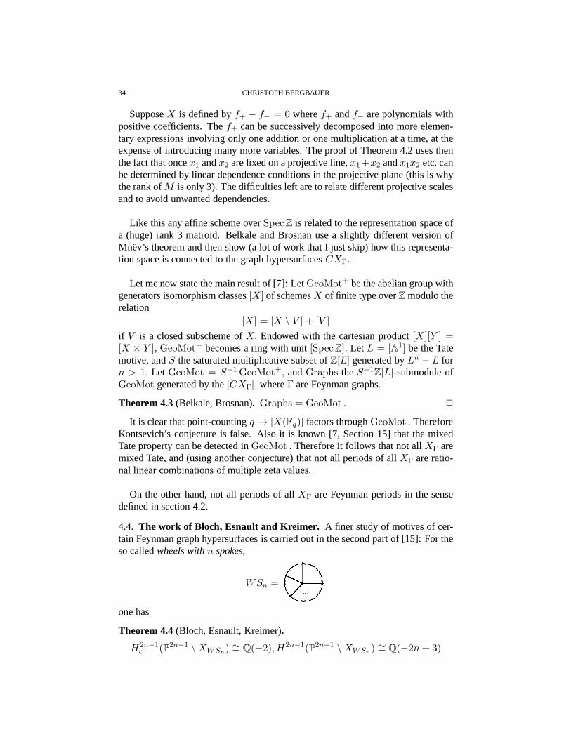
4.4. The work of Bloch, Esnault and Kreimer. A finer study of motives of cer-tain Feynman graph hypersurfaces is carried out in the second part of [15]: For theso calledwheels withn spokes,

WSn =

one has

Theorem 4.4(Bloch, Esnault, Kreimer).

H2n−1c (P2n−1 \XWSn)

∼= Q(−2),H2n−1(P2n−1 \XWSn)∼= Q(−2n+ 3)


andH2n−1dR (P2n−1 \XWSn) is generated byΩ/Ψ2

WSn.

It had been known before [21,22] that

resSWSn ∈ ζ(2n− 3)Q×

and Theorem 4.4 partially confirms that an extension

0 → Q(2n− 3) → E → Q(0) → 0

is responsible for this (see [15, Section 9],[14, Section 9]).

4.5. The work of Bloch and Kreimer on renormalization. Let us return to renor-malization. Within the parametric Feynman rules, Bloch andKreimer [16] showhow to understand renormalized non-primitive integrals using periods of alimitingmixed Hodge structure.

Limiting mixed Hodge structures arise in a situation where there is a family ofHodge structures varying over a base space, in this case a punctured diskD∗ (Forzero momentum transfer Feynman graphs this one-dimensional base space is suffi-cient). In contrast to section 3.4, the parametert ∈ D∗ does not alter the exponentof the differential form, but is rather some sort of cut-off for the chain of integra-tion.

It follows from our discussion in 3.4 that the projective integral∫

σ

Ω

Ψ2Γ

is not convergent unlessΓ is primitive (This is the reason whyresS Γ is definedonly for primitive integrals): there are poles along the exceptional divisorsELγ

corresponding to divergent subgraphsγ. In other words,∫σ

ΩΨ2

Γis not a period. But

by varying the coordinate divisor∆t (and the simplexσt sitting inside∆t) witht ∈ D∗, one has afamily of mixed Hodge structures, and for allt 6= 0 the period∫σt

ΩΨ2

Γis defined.

Bloch and Kreimer describe how to express the monodromy operation on (rel-ative) homology, in particular onσt, in terms of suitable tubes around the strataof the exceptional divisor ofZS. Winding around such a tube picks up the residuealong the stratum (see section 3.4). Since the monodromy is quasi-unipotent, itslogarithm gives a (graph-independent) nilpotent matrixN such that

(27)∫

σt

Ω

Ψ2Γ

= first row of exp(N log t/2πi)(a1, . . . , ar)t

up to a multi-valued analytic function vanishing att = 0, with a1, . . . , ar periodsof a limiting mixed Hodge structure [16].

When there is only one non-zero external momentum, sayP, the relation be-tween the regularization (27) and the renormalized integral (19), where the secondgraph polynomial must be taken into account, is easy to see. Therefore (27) also


tells about the coefficientspn(Γ) of the renormalized integral (19), and one ob-serves in the monodromy representation the same combinatorial objects (nestedsets, the Connes-Kreimer coproduct) that have guaranteed locality of countertermsin section 3.

4.6. Final remarks. Let me finish this second part of the paper by just mentioningvery briefly some other results that have been obtained in this area.

The Belkale-Brosnan theorem does not provide a specific counterexample graphto Kontsevich’s conjecture (it does provide a counterexample matroid). See [35,75]for recent developments in this direction.

The methods of [15] have been extended in [36] to other graphsthan the wheelswith spokes. Regularization and renormalization in the parametric representationis also discussed in [17,18,66].

The relation between Feynman periods and multiple zeta values as periods of themoduli space of stable genus 0 curves is studied much furtherin [24, 25]. Finallythe reader may be interested in [1–3, 13, 71] for a further study of graph hypersur-faces.

REFERENCES

[1] P. Aluffi and M. Marcolli,Algebro-geometric Feynman rules. arXiv:0811.2514.[2] P. Aluffi and M. Marcolli, Feynman motives and deletion-contraction relations.

arXiv:0907.3225.[3] P. Aluffi and M. Marcolli, Parametric Feynman integrals and determinant hypersurfaces.

arXiv:0901.2107.[4] Y. Andre, Une introduction aux motifs (Motifs purs, motifs mixtes, p´eriodes), Panoramas et

Syntheses17, SMF, 2004.[5] M. Atiyah, Resolution of singularities and divison of distributions, Comm. Pure

Appl. Math. XXIII (1970), 145–150.[6] S. Axelrod and I. M. Singer,Chern–Simons perturbation theory 2, J. Diff. Geom. 39 (1994),

173–213. hep-th/9304087.[7] P. Belkale and P. Brosnan,Matroids, motives, and a conjecture of Kontsevich, Duke

Math. J. 116(2003), no. 1, 147–188. math.AG/0012198.[8] P. Belkale and P. Brosnan,Periods and Igusa local zeta functions, Int. Math. Res. Not.49

(2003), 2655–2670. math/0302090.[9] C. Bergbauer,Combinatorial and geometric aspects of Feynman graphs and Feynman inte-

grals. PhD thesis, Freie Universitat Berlin, April 2009. Published online at http://www.diss.fu-berlin.de/diss/receive/FUDISSthesis000000010972.

[10] C. Bergbauer, R. Brunetti, and D. Kreimer,Renormalization and resolution of singularities.arXiv:0908.0633.

[11] C. Bergbauer and D. Kreimer,Hopf algebras in renormalization theory: Locality and Dyson-Schwinger equations from Hochschild cohomology, IRMA Lect. Math. Theor. Phys.10 (2006),133–164. hep-th/0506190.

[12] I. N. Bernstein and S. I. Gel’fand,Meromorphy of the functionPλ, Funkcional. Anal. i Prilozen.3 (1969), no. 1, 84–85.

[13] S. Bloch,Motives associated to sums of graphs. arXiv:0810.1313.[14] S. Bloch,Motives associated to graphs, Jpn. J. Math.2 (2007), no. 1, 165–196.[15] S. Bloch, H. Esnault, and D. Kreimer,On Motives Associated to Graph Polynomials, Com-

mun. Math. Phys.267(2006), 181–225. math.AG/0510011.


[16] S. Bloch and D. Kreimer,Mixed Hodge structures and renormalization in phyics, Commun.Number Theory Phys.2 (2008), no. 4, 637–718. arXiv:0804.4399.

[17] C. Bogner and S. Weinzierl,Resolution of singularities for multi-loop integrals, Com-put. Phys. Commun.178(2008), 596–610. arXiv:0709.4092.

[18] C. Bogner and S. Weinzierl,Periods and Feynman integrals, J. Math. Phys.50 (2009), 042302.arXiv:0711.4863.

[19] N. N. Bogolyubov and D. V. Shirkov,Introduction to the theory of quantized fields, 3rd ed.,Wiley, 1980.

[20] J. Bokowski and B. Sturmfels,Computational synthetic geometry, Lecture Notes in Mathemat-ics, vol. 1355, Springer-Verlag, Berlin, 1989.

[21] D. Broadhurst and D. Kreimer,Knots and numbers inΦ4 theory to 7 loops and beyond,Int. J. Mod. Phys.C6 (1995), 519–524. hep-ph/9504352.

[22] D. Broadhurst and D. Kreimer,Association of multiple zeta values with positive knots viafeyn-man diagrams up to 9 loops, Phys. Lett.B393(1997), 403–412. hep-th/9609128.

[23] D. Broadhurst and D. Kreimer,Exact solutions of Dyson-Schwinger equations for iteratedone-loop integrals and propagator-coupling duality, Nucl. Phys.B600 (2001), 403–422. hep-th/0012146.

[24] F. Brown,On the periods of some Feynman integrals. arXiv:0910.0114.[25] F. Brown, The massless higher-loop two-point function, Commun. Math. Phys.287 (2009),

925–958. arXiv:0804.1660.[26] F. C. S. Brown,Multiple zeta values and periods of moduli spacesM0,n, Ann. Sci.Ec. Norm.

Super. (4)42 (2009), no. 3, 371–489.[27] J. Carlson, S. Muller-Stach, and C. Peters,Period mappings and period domains, Cambridge

Studies in Advanced Mathematics, vol. 85, Cambridge University Press, Cambridge, 2003.[28] J. Collins, Renormalization, Cambridge Monographs on Mathematical Physics, Cambridge

University Press, 1984.[29] A. Connes and D. Kreimer,Hopf algebras, renormalization and noncommutative geometry,

Commun. Math. Phys.199(1998), 203–242. hep-th/9808042.[30] A. Connes and D. Kreimer,Renormalization in quantum field theory and the Riemann– Hilbert

problem I: The Hopf algebra structure of graphs and the main theorem, Comm. Math. Phys.210(2000), 249–273. hep-th/9912092.

[31] A. Connes and D. Kreimer,Renormalization in quantum field theory and the Riemann-Hilbert problem II: The beta-function, diffeomorphisms and the renormalization group, Com-mun. Math. Phys.216(2001), 215–241. hep-th/0003188.

[32] A. Connes and M. Marcolli,Noncommutative Geometry, Quantum Fields, and Motives(2007).[33] P. Cvitanovic,Field theory, Nordita, 1983.[34] C. De Concini and C. Procesi,Wonderful models of subspace arrangements, Selecta

Math. (N. S. )1 (1995), no. 3, 459–494.[35] D. Doryn. Talk given at the IHES, June 2009.[36] D. Doryn,Cohomology of graph hypersurfaces associated to certain Feynman graphs. Thesis

(2008), Universitat Duisburg-Essen. arXiv:0811.0402.[37] K. Ebrahimi-Fard, L. Guo, and D. Kreimer,Spitzer’s identity and the algebraic Birkhoff de-

composition in pQFT, J. Phys.A37 (2004), 11037–11052. hep-th/0407082.[38] H. Epstein and V. Glaser,The role of locality in perturbation theory, Annales Poincare Phys.

Theor.A19 (1973), 211.[39] P. Etingof,Note on dimensional regularization, Quantum fields and strings: a course for math-

ematicians, Vol. 1, 2 (Princeton, NJ, 1996/1997), 1999, pp.597–607.[40] L. Foissy,Systems of Dyson-Schwinger equations. arXiv:0909.0358.[41] L. Foissy,Les algebres de Hopf des arbres enracines I-II, Bull. Sci. Math.126(2002), 193–239

and 249–288.[42] K. Fredenhagen,Quantenfeldtheorie I, II; Quantenfeldtheorie auf gekrummter Raumzeit, Uni-

versity of Hamburg, http://www.desy.de/uni-th/lqp/notes.html.


[43] W. Fulton and R. MacPherson,A compactification of configuration spaces, Ann. Math.139(1994), 183–225.

[44] A. Goncharov and Y. Manin,Multiple ζ-motives and moduli spacesM0,n, Compos. Math.140(2004), no. 1, 1–14. math.AG/0204102.

[45] R. Haag,Local quantum physics, fields, particles, algebras, 2nd ed., Springer, Berlin, 1996.[46] K. Hepp, Proof of the Bogolyubov–Parasiuk theorem on renormalization, Com-

mun. Math. Phys.2 (1966), 301–326.[47] C. Itzykson and J. -B. Zuber,Quantum field theory, McGraw-Hill, 1980.[48] D. Kazhdan,Introduction to QFT, Quantum fields and strings: a course for mathematicians,

Vol. 1, 2 (Princeton, NJ, 1996/1997), 1999, pp. 377–418.[49] M. Kontsevich. Talk given at the IHES, 2003.[50] M. Kontsevich. Talk given at the Gelfand seminar, Rutgers, 1997.[51] M. Kontsevich,Feynman diagrams and low-dimensional topology, First European Congress of

Mathematics, Vol. II (Paris, 1992), 1994, pp. 97–121.[52] M. Kontsevich and D. Zagier,Periods, Mathematics Unlimited – 2001 and Beyond, 2001,

pp. 771–808.[53] D. Kreimer,On the Hopf algebra structure of perturbative quantum field theories, Adv. Theor.

Math. Phys.2 (1998), 303–334. q-alg/9707029.[54] D. Kreimer,Knots and Feynman diagrams, Cambridge University Press, 2000.[55] D. Kreimer,Anatomy of a gauge theory, Annals Phys.321(2006), 2757–2781.[56] D. Kreimer,The residues of quantum field theory: Numbers we should know, Noncommutative

Geometry and Number Theory (bonn, 2003), 2006, pp. 187–204.hep-th/0404090.[57] D. Kreimer,Dyson-Schwinger equations: from Hopf algebras to number theory, Universality

and renormalization, 2007, pp. 225–248.[58] D. Kreimer, Factorization in quantum field theory: An exercise in Hopf algebras and local

singularities, Frontiers in number theory, physics, and geometry. II, 2007, pp. 715–736. hep-th/0306020.

[59] D. Kreimer,A remark on quantum gravity, Annals Phys.323(2008), 49–60. arXiv:0705.3897.[60] D. Kreimer,Etude for linear Dyson-Schwinger equations, Traces in number theory, geometry

and quantum fields, 2008, pp. 155–160.[61] D. Kreimer and W. D. van Suijlekom,Recursive relations in the core Hopf algebra.

arXiv:0903.2849.[62] D. Kreimer and K. Yeats, An etude in non-linear Dyson-Schwinger equations,

Nucl. Phys. Proc. Suppl.160(2006), 116–121. hep-th/0605096.[63] D. Kreimer and K. Yeats,Recursion and growth estimates in renormalizable quantum field

theory, Commun. Math. Phys.279(2008), no. 2, 401–427. hep-th/0612179.[64] K. Kremnizer and M. Szczesny,Feynman graphs, rooted trees, and Ringel-Hall algebras,

Comm. Math. Phys.289(2009), no. 2, 561–577.[65] L. Lafforgue,Chirugie des grassmanniennes, CRM Monograph Series, vol. 19, AMS, Provi-

dence, RI, 2003.[66] M. Marcolli, Motivic renormalization and singularities. arXiv:0804.4824.[67] I. Mencattini and D. Kreimer,The structure of the Ladder Insertion-Elimination Lie algebra,

Commun. Math. Phys.259(2005), 413–432. math-ph/0408053.[68] N. E. Mnev,Varieties of combinatorial types of projective configurations and convex polyhedra,

Dokl. Akad. Nauk SSSR283(1985), no. 6, 1312–1314.[69] N. E. Mnev,The universality theorems on the classification problem of configuration varieties

and convex polytopes varieties, Topology and geometry—Rohlin Seminar, 1988, pp. 527–543.[70] K. Osterwalder and R. Schrader,Axioms for Euclidean Green’s functions I and II, Com-

mun. Math. Phys.31 (1973), 83–112. and42 (1975) 281.[71] E. Patterson,On the singular structure of graph hypersurfaces. arXiv:1004.5166.[72] M. Reed and B. Simon,Fourier analysis, self-adjointness, Methods of modern mathematical

physics, vol. 2, Academic Press, New York, 1975.


[73] J. Richter-Gebert,Mnev’s universality theorem revisited, Sem. Lothar. Combin.34 (1995), Art.B34h, approx. 15 pp. (electronic).

[74] V. Rivasseau,From Perturbative to Constructive Renormalization, Princeton University Press,1991.

[75] O. Schnetz,Quantum field theory overFq . arXiv:0909.0905.[76] O. Schnetz,Quantum periods: A census ofφ4-transcendentals. arXiv:0801.2856.[77] R. F. Streater and A. S. Wightman,PCT, Spin and Statistics, and All That, Princeton, reprint

2000.[78] W. van Suijlekom,The Hopf algebra of Feynman graphs in QED, Lett. Math. Phys.77 (2006),

265–281. hep-th/0602126.[79] M. Szczesny,On the structure and representations of the insertion-elimination Lie algebra,

Lett. Math. Phys.84 (2008), no. 1, 65–74.[80] M. Szczesny,Hecke correspondences and Feynman graphs, Comm. Number Theory and Phys.

4 (2010).[81] A. Usnich. Private communication.[82] G. van Baalen, D. Kreimer, D. Uminsky, and K. Yeats,The QED beta-function from global

solutions to Dyson- Schwinger equations, Ann. Phys324(2009), 205–219. arXiv:0805.0826.[83] G. van Baalen, D. Kreimer, D. Uminsky, and K. Yeats,The QCD beta-function from global

solutions to Dyson- Schwinger equations, Ann. Phys.325(2010), 300–324. arXiv:0906.1754.[84] W. van Suijlekom,Multiplicative renormalization and Hopf algebras. arXiv:0707.0555.[85] W. D. van Suijlekom,Renormalization of gauge fields: A Hopf algebra approach, Com-

mun. Math. Phys.276(2007), 773–798. hep-th/0610137.[86] M. J. G. Veltman,Diagrammatica: The Path to Feynman rules. Cambridge, UK: Univ. Pr.

(1994) 284 p. (Cambridge lecture notes in physics, 4).[87] S. Weinberg,The Quantum Theory of Fields I, Cambridge University Press, 1985.[88] K. Yeats,Growth estimates for Dyson-Schwinger equations. Thesis, Boston University (2008).

arXiv:0810.2249.[89] W. Zimmermann,Convergence of Bogolyubov’s method of renormalization in momentum

space, Commun. Math. Phys.15 (1969), 208–234.

SFB 45, INSTITUT FUR MATHEMATIK , JOHANNES-GUTENBERG-UNIVERSITAT MAINZ

E-mail address: [email protected]

Documents

NOTES ON FEYNMAN INTEGRALS AND RENORMALIZATION ON FEYNMAN INTEGRALS AND RENORMALIZATION 3 2. FEYNMAN GRAPHS AND FEYNMAN INTEGRALS For the purpose of this paper, a Feynman graph is