Feynman rules for Coulomb gauge QCD

A. Andrasi a, J. C. Taylor b

July 17, 2018

a Rudjer Boskovic Institute, Zagreb, Croatiab Department of Applied Mathematics and Theoretical Physics, University

of Cambridge, Cambridge, UKKeywords: Coulomb gauge, QCD, renormalization

Abstract

The Coulomb gauge in nonabelian gauge theories is attractive in principle, butbeset with technical difficulties in perturbation theory. In addition to ordinaryFeynman integrals, there are, at 2-loop order, Christ-Lee (CL) terms, derivedeither by correctly ordering the operators in the Hamiltonian, or by resolvingambiguous Feynman integrals. Renormalization theory depends on the sub-graph structure of ordinary Feynman graphs. The CL terms do not have asub-graph sructure. We show how to carry out renormalization in the presenceof CL terms, by re-expressing these as ‘pseudo-Feynman’ integrals. We alsoexplain how energy divergences cancel.

1 Introduction

There are some reasons to be interested in the Coulomb gauge in QCD. It is theonly explicitly unitary gauge (we discount axial gauges, which have undefineddenominators 1/(n.k)1). It may be useful for bound-state problems. It hasbeen used in lattice simulations, and it has been made the basis for a discussionof confinement [1], [2], [3], [4], [5], [6], [7], [8], [13], [9], [10],[11] (the existenceof a Hamiltonian allows the use of a variational principle [12]). But there arecomplications in formulating correct Feynman rules, all concerned with the con-vergence of integrals over the energy-components of internal energy-momentumvariables. These problems are eased by using the Hamitonian (phase-space)formulation, in which the electric field Ea is one of the dynamical variables[14]. The Lagrangian in the Hamiltonian formalism, and the Feynman rules arestated in Appendix A.

1We include here the temporal gauge, in which n is time-like, although this gauge issometimes taken as a starting point.

1

arX

iv:1

204.

1722

v2 [

hep-

th]

29

May

201

2

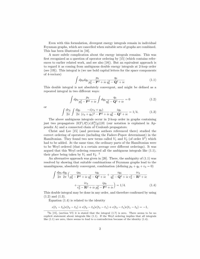
Even with this formulation, divergent energy integrals remain in individualFeynman graphs, which are cancelled when suitable sets of graphs are combined.This has been illustrated in [16].

A more subtle complication about the energy integrals remains. This wasfirst recognized as a question of operator ordering by [15] (which contains refer-ences to earlier related work, and see also [18]). But an equivalent approach isto regard it as coming from ambiguous double energy integrals at 2-loop order(see [19]). This integral is (we use bold capital letters for the space componentsof 4-vectors) ∫

dp0dq0p0

p20 −P2 + iε

q0q20 −Q2 + iε

(1.1)

This double integral is not absolutely convergent, and might be defined as arepeated integral in two different ways:∫

dp0p0

p20 −P2 + iε

∫dq0

q0q20 −Q2 + iε

= 0 (1.2)

or ∫dr02π

∫dq02π

−i(r0 + q0)

(r0 + q0)2 −P2 + iε

iq0q20 −Q2 + iε

= 1/4. (1.3)

The above ambiguous integrals occur in 2-loop order in graphs containingjust two propagators 〈0|T (Aai (x)Ebj (y))|0〉 (our notation is explained in Ap-pendix A) and a connected chain of Coulomb propagators.

Christ and Lee [15] (and previous authors referenced there) studied thecorrect ordering of operators (including the Fadeev-Popov determinant) in theHamiltonian. They found two new terms called V1 and V2 (of order h2) whichhad to be added. At the same time, the ordinary parts of the Hamiltonian wereto be Weyl ordered (that is a certain average over different orderings). It wasargued that this Weyl ordering removed all the ambiguous integrals like (1.1),their place being taken by V1 and V2. 2

An alternative approach was given in [20]. There, the ambiguity of (1.1) wasresolved by showing that suitable combinations of Feynman graphs lead to theunambiguous, absolutely convergent, combination (defining p0 + q0 + r0 = 0)∫

dp02π

dq02π

( ip0p20 −P2 + iε

iq0q20 −Q2 + iε

+iq0

q20 −Q2 + iε

ir0r20 −R2 + iε

+ir0

r20 −R2 + iε

ip0p20 −P2 + iε

)= 1/4. (1.4)

This double integral may be done in any order, and therefore confirmed by using(1.2) and (1.3).

Equation (1.4) is related to the identity

ε(t1 − t2)ε(t2 − t3) + ε(t2 − t3)ε(t3 − t1) + ε(t3 − t1)ε(t1 − t2) = −1,

2In [15], (section VI) it is stated that the integral (1.7) is zero. There seems to be noexplicit statement about integrals like (1.1). If the Weyl ordering implies that all integralslike (1.1) are zero, there seems to lead to a contradiction because of the identity (1.4).

2

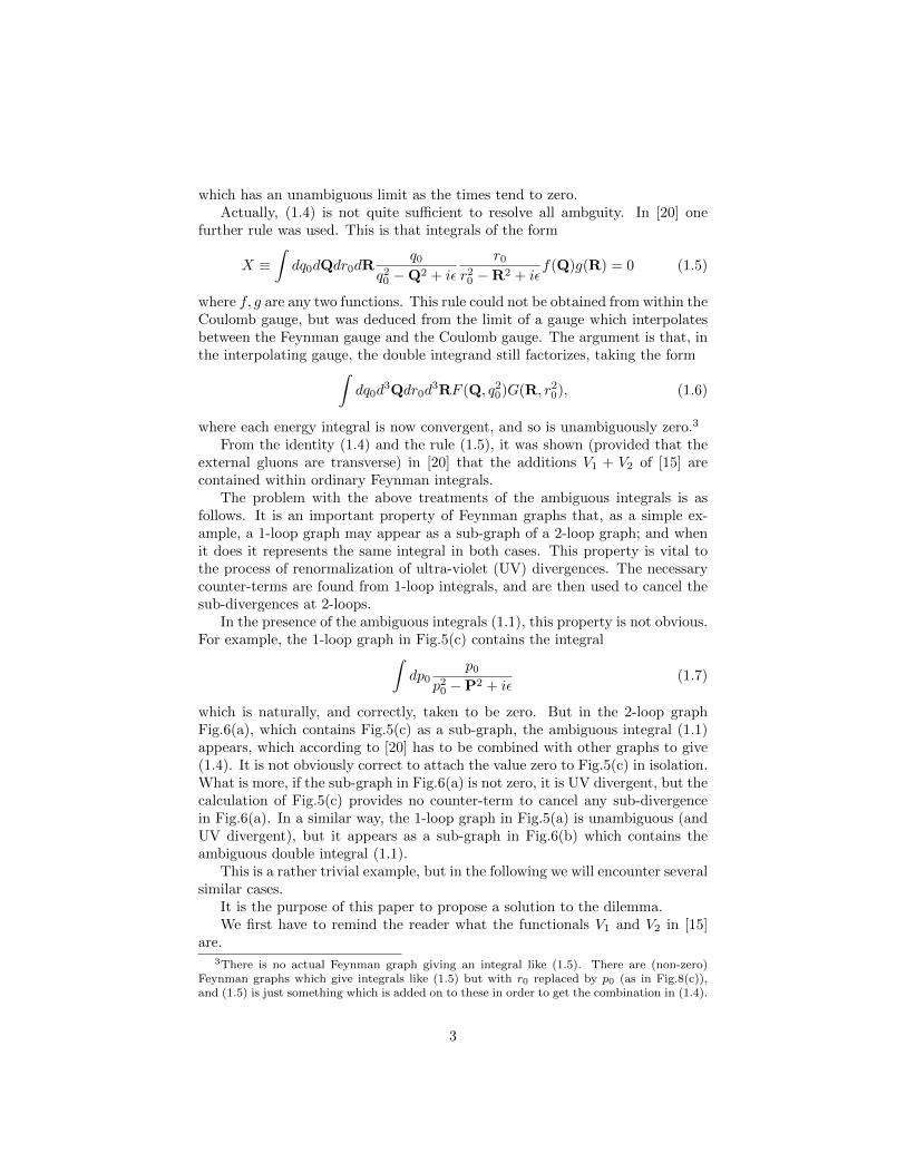
which has an unambiguous limit as the times tend to zero.Actually, (1.4) is not quite sufficient to resolve all ambguity. In [20] one

further rule was used. This is that integrals of the form

X ≡∫dq0dQdr0dR

q0q20 −Q2 + iε

r0r20 −R2 + iε

f(Q)g(R) = 0 (1.5)

where f, g are any two functions. This rule could not be obtained from within theCoulomb gauge, but was deduced from the limit of a gauge which interpolatesbetween the Feynman gauge and the Coulomb gauge. The argument is that, inthe interpolating gauge, the double integrand still factorizes, taking the form∫

dq0d3Qdr0d

3RF (Q, q20)G(R, r20), (1.6)

where each energy integral is now convergent, and so is unambiguously zero.3

From the identity (1.4) and the rule (1.5), it was shown (provided that theexternal gluons are transverse) in [20] that the additions V1 + V2 of [15] arecontained within ordinary Feynman integrals.

The problem with the above treatments of the ambiguous integrals is asfollows. It is an important property of Feynman graphs that, as a simple ex-ample, a 1-loop graph may appear as a sub-graph of a 2-loop graph; and whenit does it represents the same integral in both cases. This property is vital tothe process of renormalization of ultra-violet (UV) divergences. The necessarycounter-terms are found from 1-loop integrals, and are then used to cancel thesub-divergences at 2-loops.

In the presence of the ambiguous integrals (1.1), this property is not obvious.For example, the 1-loop graph in Fig.5(c) contains the integral∫

dp0p0

p20 −P2 + iε(1.7)

which is naturally, and correctly, taken to be zero. But in the 2-loop graphFig.6(a), which contains Fig.5(c) as a sub-graph, the ambiguous integral (1.1)appears, which according to [20] has to be combined with other graphs to give(1.4). It is not obviously correct to attach the value zero to Fig.5(c) in isolation.What is more, if the sub-graph in Fig.6(a) is not zero, it is UV divergent, but thecalculation of Fig.5(c) provides no counter-term to cancel any sub-divergencein Fig.6(a). In a similar way, the 1-loop graph in Fig.5(a) is unambiguous (andUV divergent), but it appears as a sub-graph in Fig.6(b) which contains theambiguous double integral (1.1).

This is a rather trivial example, but in the following we will encounter severalsimilar cases.

It is the purpose of this paper to propose a solution to the dilemma.We first have to remind the reader what the functionals V1 and V2 in [15]

are.3There is no actual Feynman graph giving an integral like (1.5). There are (non-zero)

Feynman graphs which give integrals like (1.5) but with r0 replaced by p0 (as in Fig.8(c)),and (1.5) is just something which is added on to these in order to get the combination in (1.4).

3

2 The functionals of Christ and Lee

In order to state what these are, we first need to define the ghost propagator,G. It is defined to be the solution of the equation

(∂/∂Xi)(Dabi (X)Gbc(X,X′;A)

)= δacδ3(X−X′). (2.1)

Here i, j, .. are 3-vector indices, a, b, .. are colour indices, we write a 4-vectorxµ = (t,Xi), and Dab

i is defined in (A3). In (2.1), Aai (x) is an external gluonfield which is transverse, ∂Aai (x)/∂Xi = 0. G is a functional of Aai . Note that(2.1) is an instantaneous equation, there are no time derivatives. It is convenientto define also

Gabi (X,X′;A) ≡ (∂/∂Xi)Gab(X,X′;A). (2.2)

The zeroth order term in the perturbation expansion ofG is just the Coulombpotential

Gab = δab1

4π

1

|X−X′|+O(g) ≡ δabG0(X−X′) +O(g). (2.3)

In terms of the ghost propagator, the complete Coulomb potential operatoris

Cab(X,X′;A) =

∫d3X′′Gcai (X′′,X;A)Gcbi (X′′,X′;A). (2.4)

We need also to define the transverse projection operator

Tij(X,Y) = δijδ3(X−Y)− ∂i∂jG0(X−Y). (2.5)

With this notation, the first Christ-Lee conribution to the Hamiltonian is

V1 = −(g2/8)fabcfa′b′c′

∫d3Xd3Y

×Gaa′

i (X,Y;A)δ3(X−Y)δbb′Gc

′ci (Y,X;A) (2.6)

For the second, we first define

Labij (X,Y;A) ≡ δabT ij(X,Y) + g

∫d3ZGaci (X,Z;A)f cbeAek(Z)Tkj(Z,Y)

(2.7)Then

V2 = −(g2/8)fabcfa′b′c′

∫dXdYLaa

′

ij (X,Y;A)Cbb′(X,Y;A)Lc

′cji (Y,X;A).

(2.8)Here we have not used the original form in [15] but an equivalent given by [20]in his equation (4.5.3).

The contributions to (2.6) and (2.8) in a perturbation series may be rep-resented by 3-dimensonal Feynman graphs, in terms of the Fourier transform

4

r p

(a)

C

q

(b)

Figure 1: Three-dimensional graphs of order g6 in momentum space. (a) anexample of a contribution to V1 in (2.6). (b) an example of a contribution toV2 in (2.8). The central chain of lines is from C in (2.4) and we call this theC-chain. The two side chains are each from L. The zig-zag line denotes (theFourier transform of) Tij . The symbol C on the central segment in (b) drawsattention to the Coulomb propagator G0 in (2.3), which in this case could bein any one of three positions on the central vertical C-chain, giving three equalcontributions.

Aai (K) of Aai (X) (which we assume to satisfy K.Aa = 0 4). We shall call theseCL graphs. Typical examples, to order g6 are shown in Fig.1(a) for V1 andFig.1(b) for V2. Our graphical notation is explained in Appendix A. The rulesare like those for a Euclidean field theory in 3-dimensions.

It will be useful to have a notation for the CL terms in momentum space,like the examples in Fig.1. We will denote these integrals by V1(N) and V2(N)where N is the total number of external gluon lines. Then

−V1(N) =gN+2

(2π)6fabcfa

′bc′∫d3Pd3R

∑n,n′

Gaa′

i (P, {n})Gc′ci (R, {n′})

≡ 1

(2π)6

∫d3Pd3RWN

1 (P,R), (2.9)

where n stands for the quantum numbers of n external gluons, that is for{Kν , iν , aν} with ν = 1, .., n and n + n′ = N . Thus Fig.1(a) is an examplewith n = n′ = 2. We have put the minus sign on the left in (2.9) because −V1,2are the contributions to the effective action.)

4This condition is assumed also in the work of Christ and Lee. Thus, unlike the contribu-tions form ordinary Feynman diagrams, the CL part of the effective action is not known fornon-transverse external gluon fields.

5

Similarly,

−V2(N) =gN+2

(2π)6fabcfa

′b′c′

×∫d3Pd3Qd3Rδ3(P+Q+R)

∑n,n′,n′′

(n′′+1)Laa′

ij (P, {n})Cbb′(R, {n′′})Lcc

′

ji (Q, {n′})

≡ 1

(2π)6

∫d3Pd3QW2(P,Q,R), (2.10)

where here n + n′ + n′′ = N . Fig.1(b) is an example with n = n′ = 1, n′′ = 2.The factor (n′′+ 1) is inserted into (2.10) to take account of the n′′+ 1 possiblepositions of the zero-order Coulomb propagator (2.3) within C (as indicated bythe ‘C’ in Fig.1(b).) In (2.10), P is defined to be the momentum through thetransverse projector {δij − (PiPj/P

2)} in L(P), and Q likewise. R is definedso that P + Q + R = 0.

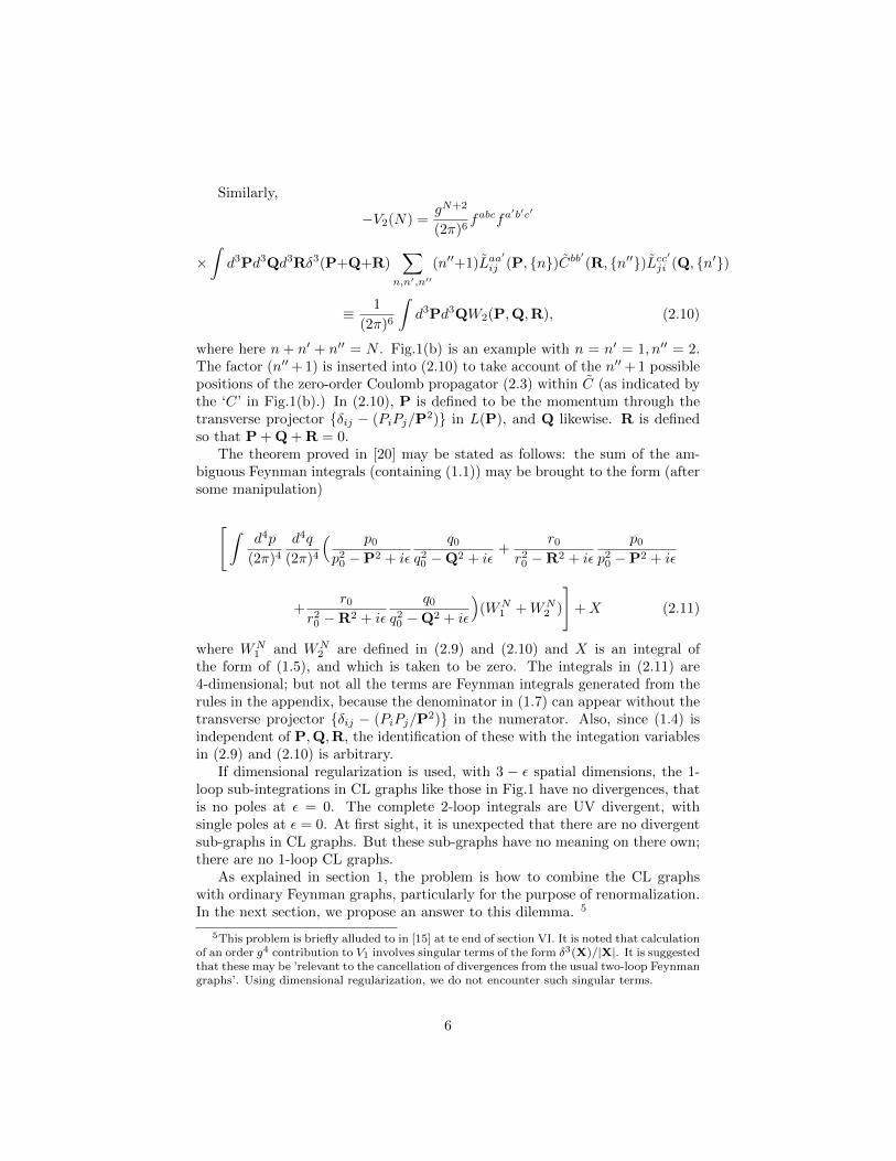
The theorem proved in [20] may be stated as follows: the sum of the am-biguous Feynman integrals (containing (1.1)) may be brought to the form (aftersome manipulation)

[∫d4p

(2π)4d4q

(2π)4

( p0p20 −P2 + iε

q0q20 −Q2 + iε

+r0

r20 −R2 + iε

p0p20 −P2 + iε

+r0

r20 −R2 + iε

q0q20 −Q2 + iε

)(WN

1 +WN2 )

]+X (2.11)

where WN1 and WN

2 are defined in (2.9) and (2.10) and X is an integral ofthe form of (1.5), and which is taken to be zero. The integrals in (2.11) are4-dimensional; but not all the terms are Feynman integrals generated from therules in the appendix, because the denominator in (1.7) can appear without thetransverse projector {δij − (PiPj/P

2)} in the numerator. Also, since (1.4) isindependent of P,Q,R, the identification of these with the integation variablesin (2.9) and (2.10) is arbitrary.

If dimensional regularization is used, with 3 − ε spatial dimensions, the 1-loop sub-integrations in CL graphs like those in Fig.1 have no divergences, thatis no poles at ε = 0. The complete 2-loop integrals are UV divergent, withsingle poles at ε = 0. At first sight, it is unexpected that there are no divergentsub-graphs in CL graphs. But these sub-graphs have no meaning on there own;there are no 1-loop CL graphs.

As explained in section 1, the problem is how to combine the CL graphswith ordinary Feynman graphs, particularly for the purpose of renormalization.In the next section, we propose an answer to this dilemma. 5

5This problem is briefly alluded to in [15] at te end of section VI. It is noted that calculationof an order g4 contribution to V1 involves singular terms of the form δ3(X)/|X|. It is suggestedthat these may be ’relevant to the cancellation of divergences from the usual two-loop Feynmangraphs’. Using dimensional regularization, we do not encounter such singular terms.

6

3 Expressing Christ-Lee terms as Feynman-likeintegrals

We want to make (2.11) more like ordinary Feynman integrals. For the WN2

term this is easy, but for the WN1 term it can only be achieved partially.

The order of the p0, q0 integrations in (2.11) is optional, because of theidentity (1.4). Let us choose the order to be that in (1.3). Then only thefirst term in the square bracket (2.11) contributes; the other two terms arezero because of equations like (1.2). Then, in the contribution from WN

2 , thereappears the correct Feynman propagtor(

δij −PiPjP2

)p0

p20 −P2 + iε, (3.1)

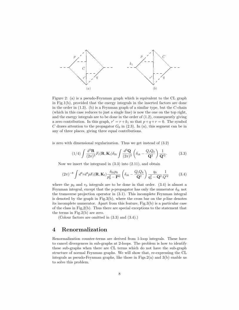
and similarly for Q. An example is shown in Fig.2(a). This looks like an ordinaryFeynman graph, but it is supplemented with the rule that the ambiguous integral(1.1) is in this case to be interpreted in the order in (1.3). Thus we are to someextent reversing the process carried out in [20]. But now we attribute the valueof (1.1) to a single type of graph, rather than to the combination in (2.11).The instantaneous propagators (denoted by dotted lines) are the same in thegraphs in Fig.2 as in the CL graph in Fig.1(b). We will call graphs like Fig.2(a)’pseudo-Feynman graphs’.

The above process does not generate any graph like the one in Fig.2(b),although this looks like an ambiguous Feynman graph. Thus we may say thatpseudo-Feynman graphs like Fig.2(b) are zero,

Note also that the above rule is consistent with the term X in (2.11) beingzero (because of (1.2)).

The general rule is that the energy integrals are to be done in the order withthe energy on the C-chain of lines (defined to be a factor like C as defined in(2.4)) last. The C-chain is the central one in Fig.2(a) but the right hand chainin Fig.2(b) (it is the chain which contains a segment with just the Coulombpropagator 1/K2)). However, there are some special exceptions to this secondrule, arising form V1.

We have not been able to express all of the WN1 in (2.11) in terms of pseudo-

Feynman graphs, but just some special parts of WN1 . But these will turn out

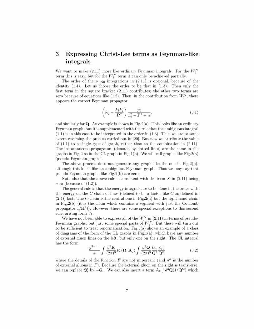
to be sufficient to treat renormalization. Fig.3(a) shows an example of a classof diagrams of the form of the CL graphs in Fig.1(a), which have any numberof external gluon lines on the left, but only one on the right. The CL integralhas the form

g3+n′′

4

∫d3R

(2π)3Fk(R,Kj)

∫d3Q

(2π)3QkQ2

Q′iQ′2

(3.2)

where the details of the function F are not important (and n′′ is the numberof external gluons in F ). Because the external gluon on the right is transverse,we can replace Q′i by −Qi. We can also insert a term δik

∫d3Q(1/Q′2) which

7

p

qr!

C

(a)

p

r!q

C

k1

(b)

Figure 2: (a) is a pseudo-Feynman graph which is equivalent to the CL graphin Fig.1(b), provided that the energy integrals in the inserted factors are donein the order in (1.3). (b) is a Feynman graph of a similar type, but the C-chain(which in this case reduces to just a single line) is now the one on the top right,and the energy integrals are to be done in the order of (1.2), consequently givinga zero contribution. In this graph, r′ = r+k1 so that p+q+r = 0. The symbolC draws attention to the propagator G0 in (2.3). In (a), this segment can be inany of three places, giving three equal contributions.

is zero with dimensional regularization. Thus we get instead of (3.2)

(1/4)

∫d3R

(2π)3Fl(R,Kl)δlk

∫d3Q

(2π)3

(δik −

QiQkQ2

)1

Q′2. (3.3)

Now we insert the integrand in (3.3) into (2.11), and obtain

(2π)−8∫d4rd4pFl(R,Kl)

δlkp0p20 −P2

(δik −

QiQkQ2

)q0

q20 −Q2

1

Q′2(3.4)

where the p0 and r0 integrals are to be done in that order. (3.4) is almost aFeynman integral, except that the p-propagator has only the numerator δlk notthe transverse projection operator in (3.1). This incomplete Feynman integralis denoted by the graph in Fig.3(b), where the cross bar on the p-line denotesits incomplete numerator. Apart from this feature, Fig.3(b) is a particular caseof the class in Fig,2(b). Thus there are special exceptions to the statement thatthe terms in Fig.2(b) are zero.

(Colour factors are omitted in (3.3) and (3.4).)

4 Renormalization

Renormalization counter-terms are derived from 1-loop integrals. These haveto cancel divergences in sub-graphs at 2-loops. The problem is how to identifythese sub-graphs when there are CL terms which do not have the sub-graphstructure of normal Feynman graphs. We will show that, re-expressing the CLintegrals as pseudo-Feynman graphs, like those in Figs.2(a) and 3(b) enable usto solve this problem.

8

r

q

(a)

p

q

(b)

r

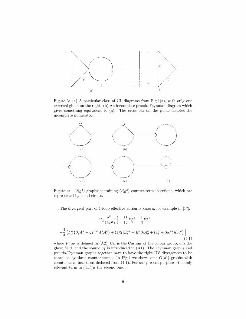
Figure 3: (a) A particular class of CL diagrams from Fig.1(a), with only oneexternal gluon on the right. (b) An incomplete pesudo-Feynman diagram whichgives something equivalent to (a). The cross bar on the p-line denotes theincomplete numerator.

(d) (e) (f)

(a) (b) (c)

Figure 4: O(g4) graphs containing O(g2) counter-term insertions, which arerepresented by small circles.

The divergent part of 1-loop effective action is known, for example in [17]:

−CGg2

16π2

1

ε

[− 11

12F aij

2 − 1

6F a0i

2

−4

3

(F a0i{∂jAai − gfabcAbiAcj}+ (1/2)Ea2i + Eai ∂iA

a0 + (uai + ∂ic

∗a)∂ica) ](4.1)

where F aµν is defined in (A2), CG is the Casimir of the colour group, c is theghost field, and the source uai is introduced in (A1). The Feynman graphs andpseudo-Feynman graphs together have to have the right UV divergences to becancelled by these counter-terms. In Fig.4 we show some O(g4) graphs withcounter-term insertions deduced from (4.1). For our present purposes, the onlyrelevant term in (4.1) is the second one.

9

(a) (b) (c)

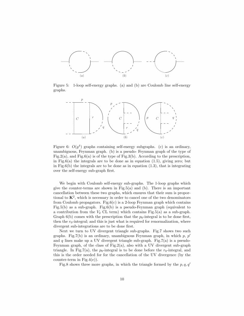
Figure 5: 1-loop self-energy graphs. (a) and (b) are Coulomb line self-energygraphs.

(a) (b) (c)

C C C

p

r

q

p

rq

p q

Figure 6: O(g4) graphs containing self-energy subgraphs. (c) is an ordinary,unambiguous, Feynman graph. (b) is a pseudo- Feynman graph of the type ofFig.2(a), and Fig.6(a) is of the type of Fig.3(b). According to the prescription,in Fig.6(a) the integrals are to be done as in equation (1.5), giving zero; butin Fig.6(b) the integrals are to be done as in equation (1.3), that is integratingover the self-energy sub-graph first.

We begin with Coulomb self-energy sub-graphs. The 1-loop graphs whichgive the counter-terms are shown in Fig.5(a) and (b). There is an importantcancellation between these two graphs, which ensures that their sum is propor-tional to K2, which is necessary in order to cancel one of the two denominatorsfrom Coulomb propagators. Fig.6(c) is a 2-loop Feynman graph which containsFig.5(b) as a sub-graph. Fig.6(b) is a pseudo-Feynman graph (equivalent toa contribution from the V2 CL term) which contains Fig.5(a) as a sub-graph.Graph 6(b) comes with the prescription that the p0-integral is to be done first,then the r0-integral; and this is just what is required for renormalization, wheredivergent sub-integrations are to be done first.

Next we turn to UV divergent triangle sub-graphs. Fig.7 shows two suchgraphs. Fig.7(b) is an ordinary, unambiguous Feynman graph, in which p, p′

and q lines make up a UV divergent triangle sub-graph. Fig.7(a) is a pseudo-Feynman graph, of the class of Fig.2(a), also with a UV divergent sub-graphtriangle. In Fig.7(a), the p0-integral is to be done before the r0-integral, andthis is the order needed for for the cancellation of the UV divergence (by thecounter-term in Fig.4(e)).

Fig.8 shows three more graphs, in which the triangle formed by the p, q, q′

10

p

qr!

C

(a)

p

r!q

C

(b)

p! p!

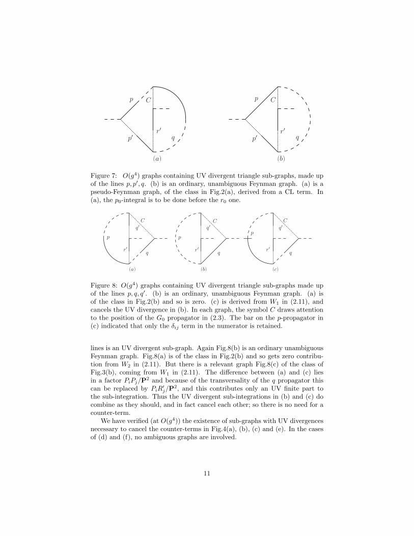
Figure 7: O(g4) graphs containing UV divergent triangle sub-graphs, made upof the lines p, p′, q. (b) is an ordinary, unambiguous Feynman graph. (a) is apseudo-Feynman graph, of the class in Fig.2(a), derived from a CL term. In(a), the p0-integral is to be done before the r0 one.

(a) (b) (c)

p

r!

q!C

q

Cq!

p

r! q

pq!C

r!q

Figure 8: O(g4) graphs containing UV divergent triangle sub-graphs made upof the lines p, q, q′. (b) is an ordinary, unambiguous Feynman graph. (a) isof the class in Fig.2(b) and so is zero. (c) is derived from W1 in (2.11), andcancels the UV divergence in (b). In each graph, the symbol C draws attentionto the position of the G0 propagator in (2.3). The bar on the p-propagator in(c) indicated that only the δij term in the numerator is retained.

lines is an UV divergent sub-graph. Again Fig.8(b) is an ordinary unambiguousFeynman graph. Fig.8(a) is of the class in Fig.2(b) and so gets zero contribu-tion from W2 in (2.11). But there is a relevant graph Fig.8(c) of the class ofFig.3(b), coming from W1 in (2.11). The difference between (a) and (c) liesin a factor PiPj/P

2 and because of the transversality of the q propagator thiscan be replaced by PiR

′j/P

2, and this contributes only an UV finite part tothe sub-integration. Thus the UV divergent sub-integrations in (b) and (c) docombine as they should, and in fact cancel each other; so there is no need for acounter-term.

We have verified (at O(g4)) the existence of sub-graphs with UV divergencesnecessary to cancel the counter-terms in Fig.4(a), (b), (c) and (e). In the casesof (d) and (f), no ambiguous graphs are involved.

11

5 Energy divergences

Another unfortunate feature of the Coulomb gauge is the presence, in individualgraphs, of energy-divergences, that is integrals of the form∫

dr0F (r0,R) (5.1)

whereF → F (R) as r0 →∞. (5.2)

Some, but not all, of these energy divergences occur in just the same graphswhich have the ambiguous integrals described in section 1, that is (to 2-loop or-der) graphs containing only two transverse gluon lines. The ambiguous integralsshow up when doing the integrals in the order∫

d3Rd3Pdr0dp0. (5.2)

The energy divergences appear from the order∫d3Rdr0d

3Pdp0 (5.3)

which is the order required by renormalization theory.It is expected that these energy divergences should cancel when sets of graphs

are combined. This has been confirmed at O(g4) in [17] but only when the sub-graphs are quark loops. Then, the O(g2) effective action is gauge-invariant,obeying Ward identities. The analysis in [17] made use of these Ward identities.We want to extend the argument to cover gluon loop sub-graphs. Then theO(g2) effective action is in general not gauge-invariant, but only BRST invariant,so it is not obvious that the cancellation of energy divergences is as simple. Thedivergent parts are shown in equation (4.1), and indeed they are not all gaugeinvariant. However, the only one relevant to the energy divergences is the secondterm in (4.1), which is gauge invariant.

The counter-term graphs in Fig.4 exhibit the energy divergences clearly, andthe 2-loop graphs whose sub-divergences Fig.4 cancel are the ones with energydivergences.

In order to extend the argument of [17] to gluon loop sub-graphs, we needto show that these sub-graphs at high energy obey Ward identities, not justBRST identities. The divergent parts obey Ward identities because the ghostgraphs shown in Fig.9 are UV convergent. In order to extend the argumentto high-energy limits, we need to verify that the graphs like those Fig.9 arealso suppressed at high energy. The graphs in Fig.9 have open ghost linesterminating at the ghost field ca and the sources ua0 , u

ai or vai , which appear in

the original Lagrangian in equation (A1) in Appendix.The graphs in Fig.9 all appear by power counting to be linearly divergent

in the UV, but they are each proportional to Pi (because the gluon line k istransverse), and so are at most logarithmically divergent. But in (b) there are

12

(a) (b)

(c) (d)

p p

p p

k

k

k k

q

q

q q

j j

j j

ui vi

vi vi

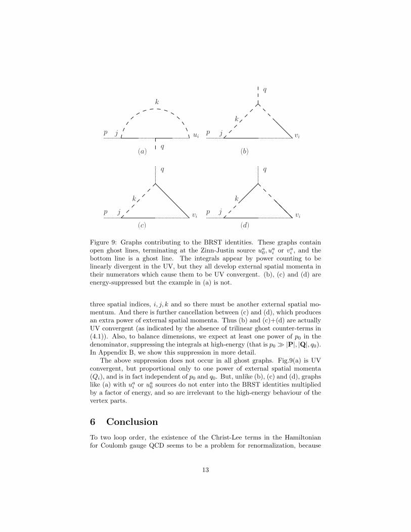
Figure 9: Graphs contributing to the BRST identities. These graphs containopen ghost lines, terminating at the Zinn-Justin source ua0 , u

ai or vai , and the

bottom line is a ghost line. The integrals appear by power counting to belinearly divergent in the UV, but they all develop external spatial momenta intheir numerators which cause them to be UV convergent. (b), (c) and (d) areenergy-suppressed but the example in (a) is not.

three spatial indices, i, j, k and so there must be another external spatial mo-mentum. And there is further cancellation between (c) and (d), which producesan extra power of external spatial momenta. Thus (b) and (c)+(d) are actuallyUV convergent (as indicated by the absence of trilinear ghost counter-terms in(4.1)). Also, to balance dimensions, we expect at least one power of p0 in thedenominator, suppressing the integrals at high-energy (that is p0 � |P|, |Q|, q0).In Appendix B, we show this suppression in more detail.

The above suppression does not occur in all ghost graphs. Fig.9(a) is UVconvergent, but proportional only to one power of external spatial momenta(Qi), and is in fact independent of p0 and q0. But, unlike (b), (c) and (d), graphslike (a) with uai or ua0 sources do not enter into the BRST identities multipliedby a factor of energy, and so are irrelevant to the high-energy behaviour of thevertex parts.

6 Conclusion

To two loop order, the existence of the Christ-Lee terms in the Hamiltonianfor Coulomb gauge QCD seems to be a problem for renormalization, because

13

they do not have sub-graph structure of ordinary Feynman graphs. We haveshown that this difficulty is overcome, by re-expressing the Christ-Lee terms aspseudo-Feynamn graphs. We have also shown how energy divergences cancelbetween Feynman and pseudo-Feynman graphs.

However, to three-loop order there may remain problems about the renor-malization of the Christ-Lee terms, when ultra-violet divergent sub-graphs areinserted into the ambiguous 2-loop graphs. This question has been discussed insection 5(ii) of [20] and in [21], [22].

This paper is only about perturbation theory. An important open questionis whether there are related complications in, for example. lattice calculations.Certainly, the Hamiltonian must be correctly ordered, and this generates CLterms.

Appendix A - Feynman rules

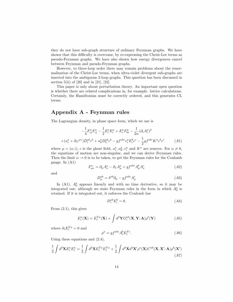
The Lagrangian density, in phase space form, which we use is

−1

4F aijF

aij −

1

2Eai E

ai + Eai F

a0i −

1

2α(∂iA

ai )2

+(uai + ∂ica∗)Dab

i cb + ua0D

ab0 c

b − gfabcvai Ebi cc −1

2gfabcKacbcc (A1)

where µ = (o, i), c is the ghost field, uai , ua0 , v

ai and Ka are sources. For α 6= 0,

the equations of motion are non-singular, and we can derive Feynman rules.Then the limit α→ 0 is to be taken, to get the Feynman rules for the Coulombgauge. In (A1)

F aµν = ∂µAaν − ∂νAaµ + gfabcAbµA

cν (A2)

andDabµ = δab∂µ − gfabcAcµ (A3)

In (A1), Aa0 appears linearly and with no time derivative, so it may beintegrated out; although we state Feynman rules in the form in which Aa0 isretained. If it is integrated out, it enforces the Coulomb law

Dabi E

bi = 0. (A4)

From (2.1), this gives

Eai (X) = ETai (X) +

∫d3YGabi (X,Y;A)ρb(Y) (A5)

where ∂iETai = 0 and

ρa = gfabcAbiETci . (A6)

Using these equations and (2.4),

1

2

∫d3XEai E

ai =

1

2

∫d2XETai ETai +

1

2

∫d3Xd3X′ρa(X)Cab(X,X′;A)ρb(X′)

(A7)

14

!ij !KiKj

K2

the transverseprojectionoperator

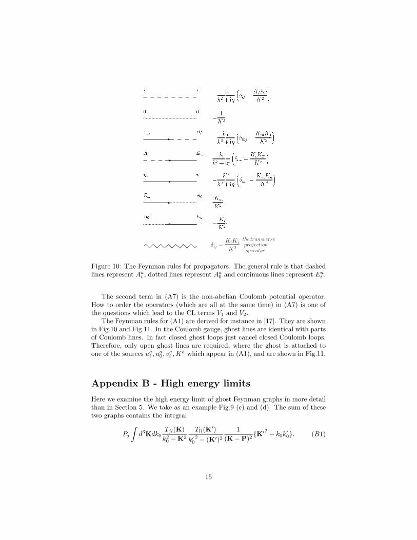
Figure 10: The Feynman rules for propagators. The general rule is that dashedlines represent Aai , dotted lines represent Aa0 and continuous lines represent Eai .

The second term in (A7) is the non-abelian Coulomb potential operator.How to order the operators (which are all at the same time) in (A7) is one ofthe questions which lead to the CL terms V1 and V2.

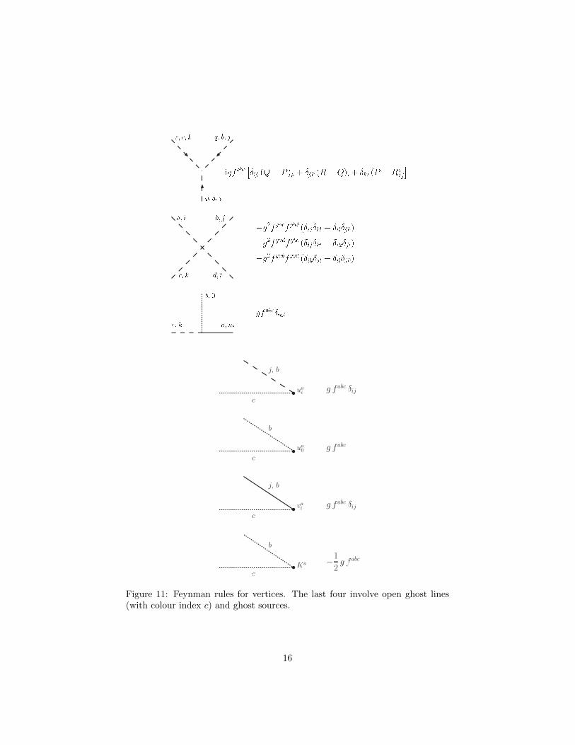
The Feynman rules for (A1) are derived for instance in [17]. They are shownin Fig.10 and Fig.11. In the Coulomb gauge, ghost lines are identical with partsof Coulomb lines. In fact closed ghost loops just cancel closed Coulomb loops.Therefore, only open ghost lines are required, where the ghost is attached toone of the sources uai , u

a0 , v

ai ,K

a which appear in (A1), and are shown in Fig.11.

Appendix B - High energy limits

Here we examine the high energy limit of ghost Feynman graphs in more detailthan in Section 5. We take as an example Fig.9 (c) and (d). The sum of thesetwo graphs contains the integral

Pj

∫d3Kdk0

Tjl(K)

k20 −K2

Tli(K′)

k′02 − (K′)2

1

(K−P)2{K′2 − k0k′0}. (B1)

15

c

c

c

c

uai

Ka

vai

ua0

j, b

b

j, b

b

g fabc !ij

!1

2g fabc

g fabc !ij

g fabc

Figure 11: Feynman rules for vertices. The last four involve open ghost lines(with colour index c) and ghost sources.

16

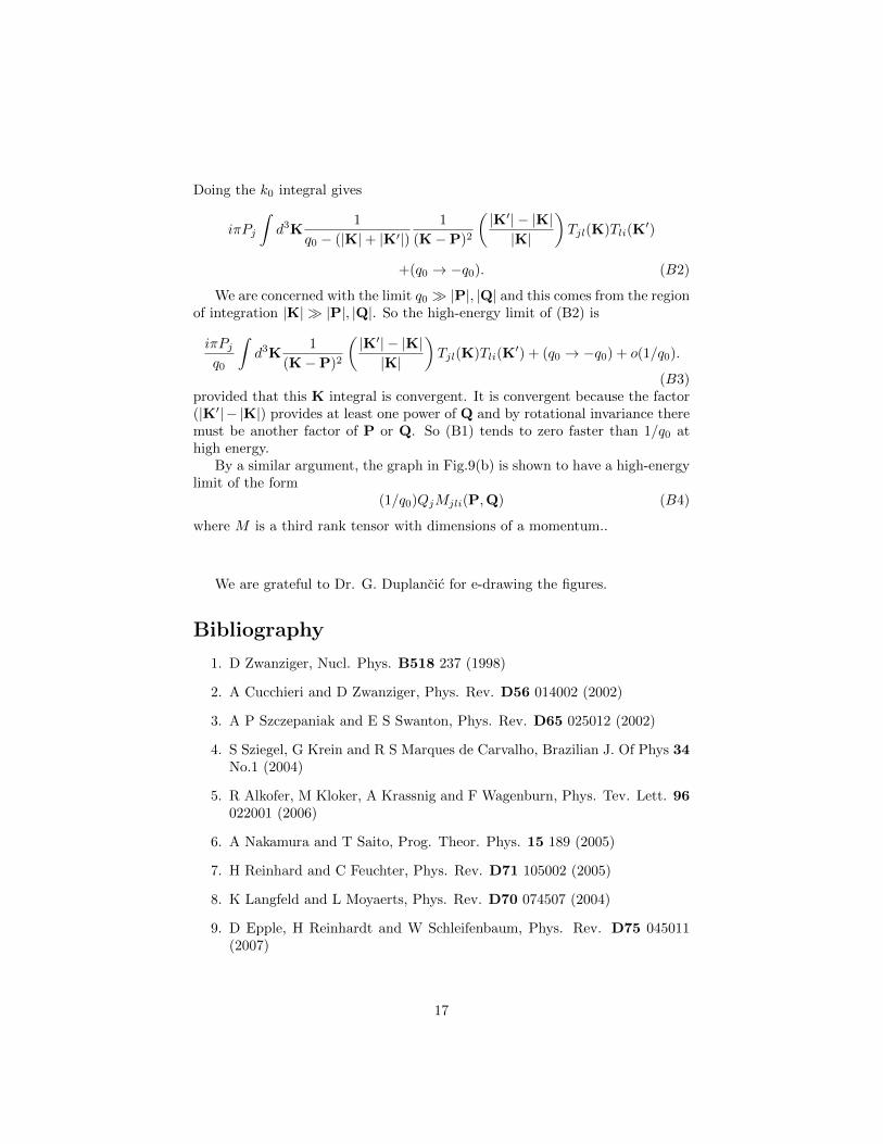
Doing the k0 integral gives

iπPj

∫d3K

1

q0 − (|K|+ |K′|)1

(K−P)2

(|K′| − |K||K|

)Tjl(K)Tli(K

′)

+(q0 → −q0). (B2)

We are concerned with the limit q0 � |P|, |Q| and this comes from the regionof integration |K| � |P|, |Q|. So the high-energy limit of (B2) is

iπPjq0

∫d3K

1

(K−P)2

(|K′| − |K||K|

)Tjl(K)Tli(K

′) + (q0 → −q0) + o(1/q0).

(B3)provided that this K integral is convergent. It is convergent because the factor(|K′|− |K|) provides at least one power of Q and by rotational invariance theremust be another factor of P or Q. So (B1) tends to zero faster than 1/q0 athigh energy.

By a similar argument, the graph in Fig.9(b) is shown to have a high-energylimit of the form

(1/q0)QjMjli(P,Q) (B4)

where M is a third rank tensor with dimensions of a momentum..

We are grateful to Dr. G. Duplancic for e-drawing the figures.

Bibliography

1. D Zwanziger, Nucl. Phys. B518 237 (1998)

2. A Cucchieri and D Zwanziger, Phys. Rev. D56 014002 (2002)

3. A P Szczepaniak and E S Swanton, Phys. Rev. D65 025012 (2002)

4. S Sziegel, G Krein and R S Marques de Carvalho, Brazilian J. Of Phys 34No.1 (2004)

5. R Alkofer, M Kloker, A Krassnig and F Wagenburn, Phys. Tev. Lett. 96022001 (2006)

6. A Nakamura and T Saito, Prog. Theor. Phys. 15 189 (2005)

7. H Reinhard and C Feuchter, Phys. Rev. D71 105002 (2005)

8. K Langfeld and L Moyaerts, Phys. Rev. D70 074507 (2004)

9. D Epple, H Reinhardt and W Schleifenbaum, Phys. Rev. D75 045011(2007)

17

10. G Burgio, M Quandt and H Reinhardt, Phys. Rev. Lett. 102 032002(2009)

11. D R Campagnari, H Reinhardt and A Weber, Phys. Rev. D80 025005(2009)

12. H Reinhardt, D R Campagnari, D Epple, M Leder, M Pak and W Schleifen-baum, arXiv 0807.4635

13. Y Nakagawa, A Voigt, E-M Ilgenfritz, M Muller-Preussker, A Nakamura,T Saito, A Sternbeck and H Toki, arXiv:0902.4321 [hep-lat] (2009)

14. R N Mohapatra, Phys. Rev D4 378 and 1007 (1971)

15. N H Christ and T D Lee, Phys. Rev. D22 939 (1980)

16. A Andrasi and J C Taylor Eur. Phys. J C 41 377 (2005)

17. A Andrasi and J C Taylor, Annals of Physics 324 2179 (2009)

18. H Cheng and E-C Tsai, Chinese Journal of Physics 25 95 (1987)

19. H Cheng and E-C Tsai, Phys. Lett B176 (1986) 130, Phys. Rev. Lett.57 511 (1986)

20. Paul Doust, Annals of Physics 177 169 (1987)

21. P J Doust and J C Taylor, Physics Letters 197 232 (1987)

22. A Andrasi and J C Taylor, Annals of Physics 326 1053 (2011)

18