Embed Size (px)
Citation preview

NOTES AND CORRESPONDENCE
A Combined Wind Profiler and Polarimetric Weather Radar Methodfor the Investigation of Precipitation and Vertical Velocities
MICHIHIRO S. TESHIBA* AND PHILLIP B. CHILSON
School of Meteorology, and Atmospheric Radar Research Center, University of Oklahoma, Norman, Oklahoma
ALEXANDER V. RYZHKOV
Atmospheric Radar Research Center, and Cooperative Institute for Mesoscale Meteorological Studies, University of Oklahoma, and
NOAA/OAR National Severe Storms Laboratory, Norman, Oklahoma
TERRY J. SCHUUR
Cooperative Institute for Mesoscale Meteorological Studies, University of Oklahoma, and NOAA/OAR National Severe Storms
Laboratory, Norman, Oklahoma
ROBERT D. PALMER
School of Meteorology, and Atmospheric Radar Research Center, University of Oklahoma, Norman, Oklahoma
(Manuscript received 18 December 2007, in final form 24 November 2008)
ABSTRACT
A method is presented by which combined S-band polarimetric weather radar and UHF wind profiler
observations of precipitation can be used to extract the properties of liquid phase hydrometeors and the
vertical velocity of the air through which they are falling. Doppler spectra, which contain the air motion
and/or fall speed of hydrometeors, are estimated using the vertically pointing wind profiler. Complementary
to these observations, spectra of rain drop size distribution (DSD) are simulated by several parameters as
related to the DSD, which are estimated through the two polarimetric parameters of radar reflectivity (ZH)
and differential reflectivity (ZDR) from the scanning weather radar. These DSDs are then mapped into
equivalent Doppler spectra (fall speeds) using an assumed relationship between the equivolume drop dia-
meter and the drop’s terminal velocity. The method is applied to a set of observations collected on 11 March
2007 in central Oklahoma. In areas of stratiform precipitation, where the vertical wind motion is expected to
be small, it was found that the fall speeds obtained from the spectra of the rain DSD agree well with those of
the Doppler velocity estimated with the profiler. For those cases when the shapes of the Doppler spectra are
found to be similar in shape but shifted in velocity, the velocity offset is attributed to vertical air motion. In
convective rainfall, the Doppler spectra of the rain DSD and the Doppler velocity can exhibit significant
differences owing to vertical air motions together with atmospheric turbulence. Overall, it was found that the
height dependencies of Doppler spectra measured by the profiler combined with vertical profiles of Z, ZDR,
and the cross correlation (rHV) as well as the estimated spectra of raindrop physical terminal fall speeds from
the polarimetric radar provide unique insight into the microphysics of precipitation. Vertical air motions
(updrafts/downdrafts) can be estimated using such combined measurements.
1. Introduction
Midlatitude mesoscale convective systems (MCSs)
have been the focus of countless studies over the past
years. These storm systems are usually characterized by
a leading convective line followed by a region of trailing
* Current affiliation: Weathernews Inc., Chiba, Japan.
Corresponding author address: Michihiro S. Teshiba, School of
Meteorology, University of Oklahoma, 120 David L. Boren Blvd.,
Rm. 5900, Norman, OK 73072-7307.
E-mail: [email protected]
1940 J O U R N A L O F A T M O S P H E R I C A N D O C E A N I C T E C H N O L O G Y VOLUME 26
DOI: 10.1175/2008JTECHA1102.1
� 2009 American Meteorological Society

stratiform precipitation. Often there is a distinct tran-
sition zone between these two regions, characterized by
reduced values of the radar reflectivity. Evaporative
cooling of the precipitation contributes to a mesoscale
downdraft below the freezing level and to the formation
of a cold pool and gust front, which can trigger addi-
tional convective cells. The system is typically fed by a
rear inflow jet. Some of the studies of midlatitude MCSs
include Smull and Houze (1987), Biggerstaff and Houze
(1991, 1993), Bluestein et al. (1994), Brandes (1990),
Houze et al. (1990), and Hane and Jorgensen (1995).
Obtaining reliable estimates of the vertical velocity within
MCSs is necessary to construct a three-dimensional
model of the flow patterns within these storms; how-
ever, the measurements are not always easy to obtain.
Although many different methods for estimating the
vertical wind component within MCSs have been de-
vised and successfully implemented, we will only con-
centrate on those involving ground-based remote sens-
ing technologies, namely, radar. These fall broadly into
the categories of single-Doppler analysis, dual-Doppler
analysis, and wind profiler techniques. There is an ex-
tensive body of literature dealing with the retrieval of
wind fields using Doppler radar, but most of these
studies focus on horizontal winds. The retrieval of the
vertical component of the wind field is more problem-
atic. As we will show, each of the proposed methods
suffers from inherent limitations.
For a single-Doppler weather radar, one can estimate
the vertical component of the three-dimensional wind
using a velocity–azimuth display (VAD) (Browning
and Wexler 1968), volume velocity processing (VVP)
(Waldteufel and Corbin 1979), or other similar tech-
niques. Each uses the assumption that the wind field is
uniform, or varies at most linearly, across the volume
scanned by the radar. Then, some form of mass conti-
nuity equation is invoked to get the vertical air motion.
In addition to these single-Doppler scanning methods,
there have also been attempts to extract vertical air
motion estimates from data obtained while the radar is
oriented vertically (Rogers 1964; Joss and Waldvogel
1970; Zawadzki et al. 2005). Here, a particular form of
the drop size distribution (DSD) and the relation be-
tween equivolume drop diameters and their terminal
fall speeds are assumed. Then, using a radar reflectivity–
rainfall rate (Z–R) relationship, the expected mean fall
speed of the observed precipitation can be estimated
from the radar reflectivity factor. The difference be-
tween the expected mean fall speed and the observed
vertical Doppler velocity gives the vertical air motion.
By incorporating data from two weather radars, we
can begin to directly investigate the three-dimensional
dynamic and thermodynamic features of storm systems
using a dual-Doppler radar analysis (Armijo 1969;
Lhermite 1970). This method has been extensively used
in the past to study the three-dimensional wind field
within MCSs. However, the ‘‘three dimensional’’ qual-
ifier most often means that estimates of the horizontal
wind in three dimensions are retrieved as opposed to the
three-dimensional wind vector itself. A few examples of
studies that do use dual-Doppler data to retrieve the
vertical wind field include Houze et al. (1989), Biggerstaff
and Houze (1993), and Braun and Houze (1994). Re-
cently, Shapiro and Mewes (1999) have presented a
new formulation for retrieving the three-dimensional
wind field using dual-Doppler radar data. Mewes and
Shapiro (2002) have specifically discussed the problems
associated with estimating the vertical velocity field
using dual-Doppler measurements and that some form
of constraining equation must be introduced. In the case
of Mewes and Shapiro (2002), the anelastic vorticity
equation is invoked as that constraint.
The main objective of this paper is to present a new
method of investigating combined observations of pre-
cipitation from polarimetric weather radars and wind
profilers. Through this method, properties of liquid
phase hydrometeors together with estimates of vertical
air motion through which the particles are falling are
retrieved. Data from the polarimetric weather radar are
used together with an empirically based model to find
estimates of the drop size distribution for the rain.
These data are used in conjunction with Doppler spec-
tra from a vertically pointing wind profiler and an as-
sumed relationship between equivolume drop diameter
and its terminal fall speed to calculate the vertical com-
ponent of the wind. The mathematical framework and
underlying assumptions incorporated into the technique
are provided in section 2. To test the method, an exper-
iment was conducted during which an MCS was observed
(see section 3). The resulting data are analyzed and
presented in section 4, and some of the inferred prop-
erties of precipitation associated with the MCS can be
found in section 5. Finally, the conclusions are outlined in
section 6.
2. Background and mathematical framework
Wind profilers are specifically designed to measure
the vertical and horizontal components of the wind field
aloft. However, it is generally difficult to distinguish be-
tween contributions of precipitation and vertical air
motion using a single UHF wind profiler. If, however,
the wind profiler operates at sufficiently long wave-
lengths, for example, VHF, both precipitation and clear-
air returns contribute to the backscattered signal and can
often be distinguished in the Doppler spectrum. Then, it
becomes trivial to measure the vertical wind; in these
SEPTEMBER 2009 N O T E S A N D C O R R E S P O N D E N C E 1941

cases, precipitation properties can also be investigated
(Fukao et al. 1985; Wakasugi et al. 1986; Rajopadhyaya
et al. 1994; Lucas et al. 2004). In some studies, two wind
profilers of different wavelengths (UHF and VHF) are
deployed (Gage et al. 1999; Cifelli et al. 2000; Schafer
et al. 2002). Then, the UHF and VHF signals can be
used primarily to measure the precipitation and clear-
air backscatter, respectively. If one is solely interested
in measuring the fall speed of the hydrometeors, then it
may be possible to simply assume that the vertical com-
ponent of the wind field is negligibly small, as is often the
case in stratiform precipitation (Williams 2002).
Unique opportunities to explore the characteristics
of rain microphysics can be achieved using comple-
mentary data from wind profilers and polarimetric
weather radars (e.g., May et al. 2001, 2002; May and
Keenan 2005). In a joint project involving the National
Oceanic and Atmospheric Administration’s National
Severe Storms Laboratory (NOAA NSSL) and the Uni-
versity of Oklahoma (OU), such measurements of pre-
cipitation are being pursued. One of the wind profilers
used in the study is a UHF radar operated through the
OU Atmospheric Radar Research Center (ARRC) and
is located at the Kessler Farm Field Laboratory (KFFL)
(Chilson et al. 2007). Another wind profiler available for
the study, which is also located at KFFL, is part of the
NOAA Profiler Network (NPN) and regularly pro-
duces estimates of the three-dimensional wind profile
(Benjamin et al. 2004). The NPN profiler also oper-
ates at UHF. Polarimetric radar data are obtained using
the research platform Weather Surveillance Radar-1988
Doppler (WSR-88D; KOUN) operated by NOAA NSSL.
Polarimetric radar data, such as those provided with
KOUN, have been shown to be an effective resource
for precipitation studies (e.g., Ryzhkov et al. 2005a,b;
Scharfenberg et al. 2005).
Radar reflectivity (ZH), differential radar reflectivity
(ZDR), and cross correlation (rHV) from the polari-
metric weather radar are used to provide information
regarding hydrometeors within the radar sampling vol-
ume (Straka et al. 2000). If the DSD of raindrops is
assumed to follow a constrained gamma distribution,
which is determined by two parameters, then these pa-
rameters can be estimated from the measurements of
ZH and ZDR (e.g., Zhang et al. 2001; Brandes et al. 2004;
Cao et al. 2008). The characteristics of hydrometeors
below and around the freezing level are studied by ex-
amining the DSDs estimated using the polarimetric
radar together with the Doppler spectra measured with
the ARRC profiler operating in a vertically pointing
mode. Horizontal wind data are provided by the NPN
profiler. An additional source of weather radar data is
the WSR-88D located near Oklahoma City (KTLX).
The wind retrieval algorithm used in the present study
uses estimates of the DSD from polarimetric weather
radar data together with a knowledge of the terminal
fall speed of precipitation in air. As described below,
Doppler spectra of terminal fall speeds for raindrops are
estimated using a polarimetric DSD retrieval. Compar-
ing the retrieved spectra of terminal fall speeds with the
spectra directly measured by the wind profiler allows us
to estimate the vertical velocity of the air motion. A
schematic depicting the approach is shown in Fig. 1. It is
assumed that all precipitation is liquid (no ice). There-
fore, we focus our attention below the melting layer.
a. DSD estimating algorithm
The method of estimating DSD data from polari-
metric weather radar observations used in the present
study is mainly based on the work of Cao et al. (2008).
It applies to liquid precipitation and assumes that the
underlying DSD follows a constrained gamma distri-
bution as given by
N(D) 5 NoDm exp(�LD), (1)
FIG. 1. Schematic of the data flow and algorithms used for the
radar signal processing and retrieval of the vertical wind. Squares
and ovals denote data files and data processing steps, respectively.
1942 J O U R N A L O F A T M O S P H E R I C A N D O C E A N I C T E C H N O L O G Y VOLUME 26

where D is the equivolume diameter of the raindrops
and the parameters m and L are related to one another
through the empirical equation (Cao et al. 2008)
m 5 m9(L) 1 CDZDR, (2)
where
m0(L) 5�0.0201L2 1 0.902L� 1.718, (3)
DZDR 5 ZDR � Z(a)DR, (4)
Z(a)DR 5 10 f (ZH ), (5)
f (ZH) 5�5.01710 3 10�4Z2H 1 0.07401ZH � 2.0122,
(6)
and
C 5 2. (7)
In the above equations, ZH and ZDR are expressed in
decibels and the coefficients were determined empiri-
cally. The parameter m is constrained to be within the
interval [0, 6]. The intercept parameter No can be esti-
mated through the comparison between the radar re-
flectivity from the radar and rain DSD. The radar
reflectivity is given by
ZH 5
ðN(D)D6 dD. (8)
Using this procedure, it has been possible to obtain es-
timates of the DSDs from the polarimetric weather
radar observations.
b. Vertical velocity retrieval algorithm
Having estimated DSDs from the polarimentric ob-
servations, the next step is to map these data into
equivalent Doppler spectra (fall speeds of the hydro-
meteors) using an assumed relationship between the
drop diameter and the corresponding terminal fall ve-
locity. This can be expressed mathematically as
Sn(w) 5D6N(D)
Zh
dD
dw, (9)
where Zh is given in linear units (mm6 m23), Sn(w) is the
‘‘simulated’’ normalized Doppler spectrum (e.g., Doviak
and Zrni�c 1993), and N(D) is the DSD found from ZH
and ZDR. Here, it has been assumed that the raindrop
fall speeds are related to their diameters according to
w(D) 5ro
r
� �0.4
(3.78D0.67) D # 3 mm,
5ro
r
� �0.4
[9.65� 10.3 exp(�0.6D)] D . 3 mm,
(10)
where r and ro are the atmospheric densities aloft and
at the surface, respectively. The value of the exponent
(0.4) was found empirically by Foote and du Toit (1969).
Although several different fall speed relations can be
found in the literature, it has been shown by Kanofsky
and Chilson (2008) that the estimated Doppler spec-
trum is relatively insensitive to which particular rela-
tionship is chosen.
The simulated Doppler spectrum calculated using (9)
represents the fall speeds that the drops would experi-
ence in still air. The Doppler spectra obtained from the
wind profiler, on the other hand, contain contributions
from both the particle fall speeds and the air motion.
By comparing the two sets of spectra (those estimated
from the ARRC profiler and those simulated from the
KOUN data) and assuming that the assumptions that
went into the retrievals are correct, it is possible to es-
timate the velocity of the bulk vertical air motion. That
is, for those cases when the two sets of Doppler spectra
are found to be similar in shape but shifted in velocity,
the velocity offset is attributed to the vertical air motion
(see Fig. 1).
c. Synthesized time–height intensity plot
Wind profilers typically probe the atmosphere aloft
using a combination of three or more vertically and
near-vertically oriented beams. This sampling geometry
is chosen to provide the best estimates of the three-
dimensional wind components aloft. As such, wind pro-
filers provide data as a function of height at regular time
intervals. The resulting backscattered power, for exam-
ple, can then be displayed using a time–height intensity
plot. Similar plots showing velocity and turbulence data
can also be constructed.
For the purpose of the present study, the polarimetric
weather radar (KOUN) was operated in a range–height
indicator (RHI) mode in the direction of the wind pro-
filer. It is convenient to present the polarimetric data
collected over the profiler in a time–height plane. These
observations can be directly compared with measure-
ments from the profiler. Examples of such processing
and further discussion are provided below.
3. Experimental setup and data collection
To test the method of combining data from polari-
metric weather radars and wind profilers, a special series
of measurements were conducted in central Oklahoma.
In this section we provide a brief summary of the in-
struments used and discuss how they were configured.
Two wind profilers were operated at the OU Kessler
Farm Field Laboratory, which is located approximately
30 km south of the OU campus. During precipitation
SEPTEMBER 2009 N O T E S A N D C O R R E S P O N D E N C E 1943

events, the atmosphere above the KFFL site was probed
using two S-band weather radars (see section 3b).
a. Kessler Farm Field Laboratory
The Kessler Farm Field Laboratory is a 140-ha prop-
erty that is maintained and operated by OU. KFFL
provides an ideal location for complementary mea-
surements to those obtained using the two WSR-88Ds
used in this study, since it is close enough to ensure good
resolution but far enough to be outside of the region of
ground clutter. Furthermore, KFFL offers the necessary
infrastructure to support the deployment of several in-
struments, which are needed for the study of precipi-
tation and the validation of radars. For example, OU’s
School of Meteorology operates a two-dimensional video
disdrometer and network of tipping-bucket rain gauges
at KFFL. Additionally, KFFL is host to several other
atmospheric measurement programs, which provide
atmospheric measurements that can be used for tar-
geted precipitation studies. Those programs relevant to
this discussion are the Department of Energy Atmo-
spheric Radiation Measurement Program (DOE ARM)
and the Oklahoma Mesonet.
b. Instrumentation
The two primary instruments used during this study
were an S-band polarimetric weather radar and a UHF
wind profiler (or boundary layer radar). The weather
radar is a prototype polarimetric WSR-88D used for
research and development purposes and is operated by
NOAA NSSL (Doviak et al. 2000). The wind profiler is
maintained and operated by the OU ARRC group
(Chilson et al. 2007). For the remainder of this discus-
sion, these two instruments will be simply referred to as
the KOUN and ARRC profilers, respectively.
KOUN was designed and built as a test platform for
the development and testing of algorithms intended to
improve upon current quantitative precipitation esti-
mation (QPE) methodologies. With the exception of its
polarimetric capabilities, the technical specifications of
KOUN are similar to the other WSR-88D systems
currently deployed across the United States and in other
parts of the world. That is, KOUN is an 11-cm radar
with a beamwidth of 18 and a minimum pulse width of
1.57 ms (235 m in range resolution). Using KOUN, the
effectiveness of polarimetric weather radar observa-
tions has been successfully demonstrated (e.g., Ryzhkov
et al. 2005b). Indeed, the success of KOUN has been
sufficient to convince NOAA officials to sanction the
upgrade of the national network of WSR-88Ds within the
United States to include polarization diversity (Saffle
et al. 2007).
The ARRC profiler operates at 915 MHz (corre-
sponding to a wavelength of 33 cm). The beamwidth of
the wind profiler is 98, and the beam can be directed
vertically or electronically steered along four oblique
directions having zenith angles of 228 (Carter et al.
1995). The minimum range resolution for the radar is
60 m, but a more typical mode of operation uses a range
resolution of 100–200 m. For the present study, the
ARRC profiler was operated using only a vertical beam.
Given the beamwidths, the range resolutions, and the
separation between KOUN and the ARRC profiler, the
sampling volumes of the two instruments match rela-
tively well near the surface. The ground separation be-
tween KOUN and the ARRC profiler is approximately
30 km. Taking KOUN’s lowest elevation angle of 0.58 as
an example, we find that the resulting angular resolution
and height above ground level at the location of the
ARRC profiler are 500 and 250 m, respectively. The
height of 250 m is approximately equal to the lowest
sampling volume of the ARRC profiler as configured
for this experiment. The angular resolution of the
ARRC profiler at a height of 250 m is 40 m. It should be
noted here that the two radars have been calibrated
independently. That is, the values for the radar reflec-
tivity reported in section 4 can be taken as independent
parameters.
Two additional radars are used in support of the
present study: the WSR-88D (KTLX), located near
Oklahoma City; and one of the radars in the NOAA
Profiler Network, located at KFFL. KTLX provides
continuous plan position indicator (PPI) scans and pro-
vides the overall structure of precipitating systems that
pass over KFFL. Such data are useful when diagnosing
the mesoscale environment in which the precipitation
forms. The NPN is dedicated to providing height profiles
of the three-dimensional wind vector and the virtual
temperature at several sites within the central United
States (Benjamin et al. 2004). Regrettably, the NPN
UHF radars are not capable of providing Doppler
spectra. As we discuss below, Doppler spectra from pro-
filing radars provide a means of investigating the struc-
ture and evolution of precipitation as a function of time
and height. Therefore, this radar is primarily used for
wind comparisons.
4. Observations of a mesoscale convective system
In this section, we demonstrate the utility of synthe-
sizing time–height intensity plots from RHI data and
the applicability of the vertical wind–estimating algo-
rithm described above by presenting observations of
a storm system that passed over central Oklahoma. On
11 March 2007, a low pressure system moved from west
1944 J O U R N A L O F A T M O S P H E R I C A N D O C E A N I C T E C H N O L O G Y VOLUME 26

to east across Oklahoma, which resulted in the forma-
tion of a large mesoscale convective system. The system
was characterized by the formation of a line of strong
convective clouds along a cold front, which extended in
the north–south direction. The west side of the convec-
tive line was dominated by a region of trailing stratiform
rainfall (see Fig. 2).
A typical MCS is associated with three distinct types
of precipitation: convective, stratiform, and a transition
between convective and stratiform portions (e.g., Smull
and Houze 1987; Biggerstaff and Houze 1993; Braun and
Houze 1994). Hydrometeors that form in the convec-
tive region are carried rearward by the MCSs’ midlevel,
front-to-rear flow; bridge the transition zone region; and
then grow by vapor deposition in the stratiform region
broad mesoscale updraft. Intense aggregation and melt-
ing as they fall through the freezing level result in a layer
of enhanced reflectivity that is known as the radar bright
band.
Both the ARRC and NPN profilers provided contin-
uous measurements as the system passed over KFFL.
The ARRC profiler beam was directed vertically and
the time and height resolutions during the observations
were 20 s and 200 m, respectively. Figure 3 shows time–
height intensity plots of the radar reflectivity, Doppler
velocity, and spectrum width from 1100 to 1300 UTC
for the ARRC profiler. Negative velocity values indi-
cate motion toward the radar. The observations indicate
convection in the leading edge of the storm (before 1130
UTC) and in the period between 1150 and 1210 UTC.
The precipitation was predominantly stratiform after
1210 UTC. The spectrum width data shown in the bot-
tom panel of Fig. 3 contain contributions from atmo-
spheric turbulence as well as the dispersion of fall
speeds resulting from the DSD of hydrometeors. An-
other factor influencing the spectrum width is beam
broadening. To quantify this effect, we examine the
measurements from the NPN.
Spectral broadening effects become relevant when we
later compare the Doppler spectra from the ARRC
profiler with the synthesized Doppler spectra from
KOUN. The increase of spectral width due to beam
broadening experienced by a radar depends on its beam-
width and the magnitude of the wind component trans-
verse to the beam. This contribution is given by Nastrom
(1997) and Gossard et al. (1998) as
s2 5V2
t Q2a
2 log 4, (11)
where Vt is the magnitude of the transverse wind (hor-
izontal wind in this case) and Qa is the one-way half-
power half-width of the beam, expressed in radians.
For the ARRC profiler, Qa 5 98/ffiffiffi2p
(p/1808) 5 0.111
rad. Wind data from the NPN profiler are available
during the time of this event every 6 min and extend in
height up to 16 km. Figure 4 shows four height profiles
of the horizontal wind speed observed during the storm.
The times were chosen to correspond to the four distinct
precipitation signatures selected for detailed study in
section 5. The first three profiles are generally less than
10 m s21 below 4 km. This corresponds to a contribution
to the spectral width of 0.7 m s21. For the 1230 UTC
profile, the horizontal wind speed is approximately
15 m s21 between 2 and 4 km. The corresponding con-
tribution to the spectral width is 1 m s21.
The temperature profile from the sounding data
collected for Norman, OK (OUN), at 1200 UTC on
FIG. 2. Horizontal distribution of radar reflectivity and Doppler
velocity as observed by KTLX WSR-88D for a 0.58 elevation angle
at 1200 UTC on 11 Mar 2007.
SEPTEMBER 2009 N O T E S A N D C O R R E S P O N D E N C E 1945
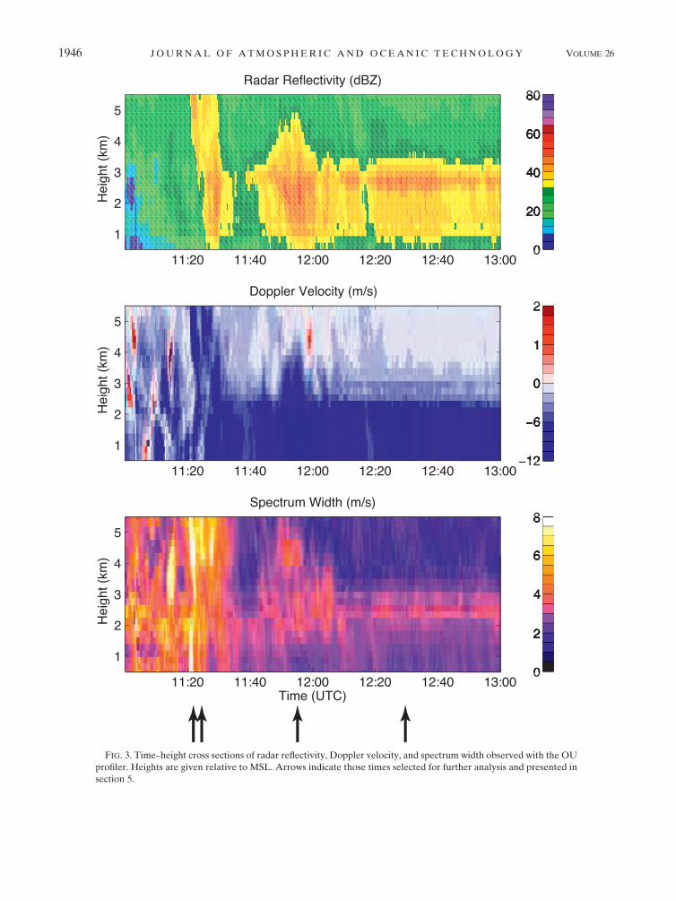
FIG. 3. Time–height cross sections of radar reflectivity, Doppler velocity, and spectrum width observed with the OU
profiler. Heights are given relative to MSL. Arrows indicate those times selected for further analysis and presented in
section 5.
1946 J O U R N A L O F A T M O S P H E R I C A N D O C E A N I C T E C H N O L O G Y VOLUME 26

11 March (not shown) indicates that the freezing level
was located at approximately 3 km MSL. This is con-
sistent with the observations from the ARRC profiler.
After 1210 UTC, the presence of a bright band can be
seen in the reflectivity plot at a height of approximately
3 km. Furthermore, there is a large change in the mag-
nitude of the observed Doppler velocities near this
height. Note that the polarimetric DSD estimation was
only applied to those KOUN data well below the freez-
ing level. The sounding data were also used to adjust the
calculated terminal fall speeds of the raindrops with
height.
KOUN was operated in an RHI scanning mode in the
direction of the two wind profilers (;1918 in azimuth)
during the MCS event. RHI data were collected from
1058 to 1444 UTC. The vertical angular resolution of
the polarimetric data was 0.18, which corresponds to
height increments of approximately 50 m above KFFL.
The RHI composite plot of ZH, ZDR, and rHV for an
azimuth angle of 1918 at time 1200 UTC is shown in Fig. 5.
In the stratiform rain region (which passed over KFFL
after approximately 1210 UTC), high reflectivity values
associated with the bright band are found at a height
of around 2.5 km. The differential reflectivity is roughly
uniform in height below a height of 2 km, and the general
shape of the DSDs are considered to be relatively similar
during that period.
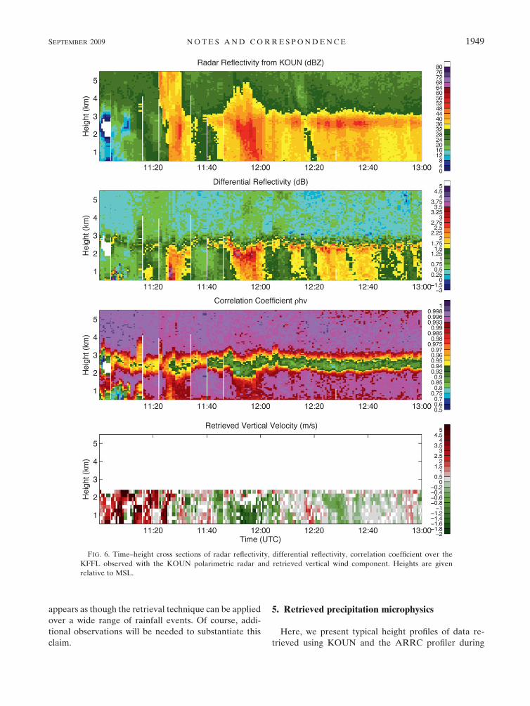
Using the method discussed above, a synthesized
time–height composite plot of ZH, ZDR, and rHV was
constructed from the RHI data over KFFL (Fig. 6). The
features in the synthesized time–height panel of the
radar reflectivity factor agree qualitatively with those
shown in Fig. 3 from the ARRC profiler. Recall that the
two radars were calibrated independently of one an-
other. The bottom panel in Fig. 6 shows the vertical
velocity data, which were retrieved using the algorithm
introduced in the previous section. As discussed below,
these wind measurements agree qualitatively with ear-
lier reports showing the wind field structures associated
with midlatitude MCSs (Houze et al. 1989; Biggerstaff
and Houze 1993; Braun and Houze 1994). In section 5
we present some examples of the combined measure-
ments from KOUN and the ARRC profiler in more
detail.
Although not a classic example of an MCS, the storm
system observed on 11 March does generally follow the
patterns associated with an MCS. A line of convective
clouds formed along the cold front and stratiform clouds
formed on the western side of the convective region. In
the convective region around 1124 UTC, a moderately
strong updraft up to 5 m s21 was observed; shortly
thereafter a region of strong reflectivity (more than
50 dBZ) was found to extend to a height of at least
5.5 km, indicative of convective squall line. The squall
line is marked by enhanced values of ZDR from a height
of 2–2.5 km to the surface, indicative of large raindrops.
Consistent with these observations, downdrafts of ap-
proximately 2 m s21 are observed below 1.5 km. The
transition from dry snow to wet snow at the top of the
melting layer is marked by a rapid increase of ZDR and a
decrease of rHV. In the presence of downdrafts associ-
ated with increased precipitation between 1150 and
1200 UTC, such a transition occurs at the lower height
levels, as Fig. 6 indicates. The stratiform portion of the
storm corresponds to those observations made after
1210 UTC. In this region the bright band is well formed
and the downdrafts are weak (approximately 1 m s21 or
less). Overall, the retrieved vertical velocity field ex-
hibits features typical of an MCS.
In an attempt to test the robustness of the method, the
similarity of these Doppler spectra of the KOUN weather
radar and ARRC profiler have been compared against
each other. Figure 7 shows the root-mean-square error
(RMSE) of these Doppler spectra in decibels at each
height and time as it relates to the reflectivity of the
KOUN radar. As shown in Eq. (10), the terminal fall
speed of raindrops asymptotically approaches a value of
9.6 m s21; therefore, only portions of the Doppler
spectra could be correctly estimated. Equation (10) has
been obtained based on ground-base observations;
however, in this paper, we considered these portions
of the spectra to have been correctly estimated, and
the RMSE is calculated based on these estimates.
Since fluctuations in the vertical wind differ according to
the type of rainfall being observed, the data have been
FIG. 4. Height profiles of the horizontal wind speed observed
with the NOAA 404-MHz profiler at 1118 (solid line), 1124
(dotted–dashed line), 1154 (dotted line), and 1230 UTC (dashed
line). Heights are given relative to MSL.
SEPTEMBER 2009 N O T E S A N D C O R R E S P O N D E N C E 1947

grouped according to convective (1058–1130 UTC),
transition (1130–1204 UTC), and stratiform (1204–1445
UTC) regions. Heights for the calculation were all
taken below 1.77 km MSL. As shown in Fig. 7, the
RMSE is generally below 3 dB for all cases. In the
stratiform rainfall region, the RMSE is approximately
1 dB. There is no clear reflectivity dependence for
the RMSE calculated for any of the cases; therefore, it
FIG. 5. Range–height cross sections of ZH, ZDR, and rHV of KOUN at 1200 UTC. KFFL is located 30 km in range
from KOUN.
1948 J O U R N A L O F A T M O S P H E R I C A N D O C E A N I C T E C H N O L O G Y VOLUME 26
appears as though the retrieval technique can be applied
over a wide range of rainfall events. Of course, addi-
tional observations will be needed to substantiate this
claim.
5. Retrieved precipitation microphysics
Here, we present typical height profiles of data re-
trieved using KOUN and the ARRC profiler during
FIG. 6. Time–height cross sections of radar reflectivity, differential reflectivity, correlation coefficient over the
KFFL observed with the KOUN polarimetric radar and retrieved vertical wind component. Heights are given
relative to MSL.
SEPTEMBER 2009 N O T E S A N D C O R R E S P O N D E N C E 1949

different phases of the MCS as it passed over KFFL.
Properties of hydrometeors are found through the po-
larimetric variables of Z, ZDR, and rHV, and tempera-
ture profiles at the KOUN sounding station, as shown
in Straka et al. (2000). For each of the selected cases,
vertical profiles of Z, ZDR, and rHV together with the
Doppler spectra from KOUN and the profiler are shown.
The Doppler spectra have all been normalized to their
peak values. For the sake of comparison, the vertical
spacing of KOUN spectral data has been matched to the
range resolution of the ARRC profiler (200 m). The
four examples presented below were selected as being
characteristic of the different stages of cloud and pre-
cipitation development within the MCS. A brief spec-
ulative account of the underlying physical processes
contributing to the observations is provided for each of
the four cases. Data from other available observations
are still being studied to construct a more comprehen-
sive analysis of the 11 March MCS. Although the ex-
planations of the examples provided below remain to be
verified, they do form a plausible and self-consistent
picture of the MCS. Similar results can be found, for
example, in Houze et al. (1989), Biggerstaff and Houze
(1993), Bluestein et al. (1994), and Braun and Houze
(1994). Furthermore, these examples illustrate the util-
ity of combined profiler and polarimetric weather radar
observations to study precipitation.
a. Early development of precipitation aloft—Heightsexceeding 4 km (1122 UTC)
The presence of large graupel is manifested by large
terminal velocities measured by the profiler and high
radar reflectivity (well over 40 dBZ) at altitudes above
4 km (see Fig. 8). The presence of strong downdrafts
is not likely at such heights, and substantial negative
velocities above 4 km are associated with the fall of
graupel/small hail (Straka et al. 2000). The hydrome-
teors in the lower portion of the cloud are quite differ-
ent than those aloft, as demonstrated by the sudden
drop in the magnitude of ZH and the fall velocities be-
low 4 km. Most likely, small-sized dry and melting
graupel was dominant within the height interval be-
tween 2.3 and 3.4 km. It seems that there is no con-
nection between this small-sized graupel and the large
graupel/hail aloft. In other words, these two species
of graupel might have been advected from different
parts of the cloud. Raindrops with relatively small sizes
below the melting layer most likely resulted from melting
FIG. 7. RMSE of the two Doppler spectra corresponding to data for KOUN and the ARRC
profiler as related to the reflectivity of KOUN: (a) all cases, (b) convective region, (c) transition
region, and (d) stratiform region. Points in the scatterplots were calculated for every time and
height believed to represent measurements of liquid phase precipitation.
1950 J O U R N A L O F A T M O S P H E R I C A N D O C E A N I C T E C H N O L O G Y VOLUME 26

graupel. Another possible explanation is that at 1122
UTC, large graupel/hail formed aloft and did not have
time to fall below the 4-km level. Tilting of the re-
flectivity core might be an alternative explanation. Note
that the melting layer is marked by the decrease in rHV
and by the rapid change of ZDR within the height in-
terval between 2.5 and 3 km. The ZDR maximum and
rHV minimum are relatively weak in the melting layer,
which also points to the melting of smaller-sized graupel.
b. Strong updraft at lower levels (1124 UTC)
At this time, the updraft portion of the system passed
over the profiler (see Fig. 9). The updraft at the levels
0.5–2.5 km is revealed by the striking differences be-
tween the spectra of vertical velocities estimated from
KOUN and those measured by the profiler. The strength
of the updraft in this case is approximately 6 m s21.
Another indication of the updraft below 2.5 km is the
combination of low ZH (of approximately 30 dBZ) and
relatively high ZDR (up to 2 dB at this time and above
4 dB 1–2 min later), which points to substantial size
sorting of raindrops; that is, raindrops with terminal
velocities less than 6 m s21 do not fall through the up-
draft. At higher levels, the situation is quite similar to
the one previously discussed (1122 UTC in section 5a),
but ZH is lower and the corresponding terminal fall
speeds are lower.
c. Convective downdraft (1155 UTC)
A classic signature of a convective downdraft within
the main precipitation shaft is observed at this time (see
Fig. 10). A bulk of precipitation descends, hence larger
ZH is observed at lower levels below 3 km. Convective
rain below the melting layer originates from melting
graupel/small hail, which has relatively high terminal
velocities immediately above the melting layer. Near
FIG. 8. Vertical profiles of Z, ZDR, and rHV; spectra of the particle fall speeds and Doppler velocity; and retrieved vertical wind
component at 1122 UTC. The radar reflectivity profiles of KOUN and the profiler are shown in the same axis. The spectra of estimated
(KOUN), measured (profiler), and fitted velocities are indicated in dark solid, light solid, and dashed lines, respectively. The retrieved
spectra are only shown for heights up to 2.5 km (well below the freezing level). Heights are given relative to MSL.
SEPTEMBER 2009 N O T E S A N D C O R R E S P O N D E N C E 1951

the ground, the difference between modal values of
KOUN and the profiler spectra corresponds to a down-
draft of approximately 2 m s21, which is likely generated
by melting graupel/hail. The downdraft combined with
cooling due to melting results in a depression of the
melting layer height (it is pushed closer to the ground),
as indicated by the vertical profiles of ZDR and rHV (see
Fig. 6). As a result, complete melting of graupel/hail
occurs at a height slightly above 1.5 km (with the freezing
level at 3 km in the ambient air).
d. Stratiform rain—Vertical motions are negligible(1231 UTC)
These data indicate a classic signature of the bright
band generated by melting snowflakes (see Fig. 11).
There is no graupel aloft, and the difference between
the terminal velocities of aggregated snowflakes above
the freezing level and the raindrops below is large. The
minimum in the vertical profile of rHV is deeper, nar-
rower, and higher compared to the situation of convec-
tive downdraft. The spectra of vertical velocities esti-
mated from the polarimetric radar and those measured
with the wind profiler agree remarkably well. This may
serve as indirect evidence of the high quality of polari-
metric DSD estimation used in this study. We must keep
in mind that the Doppler spectra from the ARRC
profiler are subject to turbulence. This is not the case for
the synthesized Doppler spectra from KOUN.
6. Conclusions
Investigations of the microphysical processes of pre-
cipitation formation can be greatly facilitated through
the combined use of wind profiler and polarimetric
weather radar data (May et al. 2001, 2002; May and
Keenan 2005). When oriented vertically, Doppler spec-
tra from the wind profiler can be used to directly measure
the vertical velocities of the sampled precipitation par-
ticles. The height dependencies of Doppler spectra
measured by the profiler combined with the vertical
profiles of ZH, ZDR, and rHV as well as the estimated
spectra of raindrop physical terminal fall speeds from
FIG. 9. Same as in Fig. 8, but for 1124 UTC.
1952 J O U R N A L O F A T M O S P H E R I C A N D O C E A N I C T E C H N O L O G Y VOLUME 26

polarimetric radar provide unique insight into the mi-
crophysics of precipitation. For example, these mea-
surements facilitate a detailed study of precipitation
processes in and around the melting layer. For this
particular case of raindrops, the polarimetric observ-
ables ZH and ZDR are used to estimate the underlying
DSD based on a constrained gamma model. Then, using
an assumed fall-speed relationship, the DSD can be
mapped into an equivalent spectrum of reflectivity-
weighted vertical velocities. These data can be directly
compared to the observed spectrum of particle fall ve-
locities measured with a profiling radar. As such, ver-
tical air motions (updrafts/downdrafts) can be estimated
using the combined measurements.
The method is being implemented in central Okla-
homa using data from KOUN and KTLX in conjunc-
tion with measurements from the ARRC and NPN
profilers (both located at KFFL). The separation be-
tween KOUN and the two profilers is only 30 km;
therefore, the sampling volumes for KOUN and the OU
profiler are similar.
An example of data collected for an MCS event has
been presented. In particular, four cases representative
of different stages of cloud and precipitation develop-
ment within the MCS have been discussed in some de-
tail. The analysis of these data is still ongoing; however,
the following examples have been shown:
d Stacked profiles of the vertical velocity spectra esti-
mated from KOUN for raindrops show remarkable
agreement with those directly measured with the
ARRC profiler during stratiform precipitation when
vertical air motions are negligible.d In some cases, the spectra from KOUN and the
ARRC profiler agreed well in shape but were offset in
velocity, which is attributed to vertical air motion.d Updrafts as large as 6 m s21 were present near the
leading edge of the MCS, which resulted in significant
size sorting of the raindrops.d Melting graupel/hail below the melting level was likely
responsible for an observed convective downdraft of
2 m s21.
FIG. 10. Same as in Fig. 8, but for 1155 UTC.
SEPTEMBER 2009 N O T E S A N D C O R R E S P O N D E N C E 1953

Admittedly, the data presented here require further
analysis to better understand the dynamic structure of
the 11 March MCS. To this end, supporting data from
the other available instrumentation will be used. Nev-
ertheless, a plausible and self-consistent characteriza-
tion of the storm event is already beginning to evolve
based on the measurements that have been shown and
discussed.
Acknowledgments. Funding for Alexander Ryzhkov
and Terry Schuur was provided by NOAA/Office of
Oceanic and Atmospheric Research under NOAA/
University of Oklahoma Agreement #NA17RJ1227,
U.S. Department of Commerce.
REFERENCES
Armijo, L., 1969: A theory for the determination of wind and
precipitation velocities with Doppler radars. J. Atmos. Sci., 26,
570–573.
Benjamin, S. G., B. E. Schwartz, E. J. Szoke, and S. E. Koch, 2004:
The value of wind profiler data in U.S. weather forecasting.
Bull. Amer. Meteor. Soc., 85, 1871–1886.
Biggerstaff, M. I., and R. A. Houze, Jr., 1991: Midlevel vorticity
structure of the 10–11 June 1985 squall line. Mon. Wea. Rev.,
119, 3066–3079.
——, and ——, 1993: Kinematics and microphysics of the transi-
tion zone of the 10–11 June 1985 squall line. J. Atmos. Sci., 50,
3091–3110.
Bluestein, H. B., S. D. Hrebenach, C.-F. Chang, and E. A. Brandes,
1994: Synthetic dual-Doppler analysis of mesoscale convec-
tive systems. Mon. Wea. Rev., 122, 2105–2124.
Brandes, E. A., 1990: Evolution and structure of the 6–7 May 1985
mesoscale convective system and associated vortex. Mon.
Wea. Rev., 118, 109–127.
——, G. Zhang, and J. Vivekanandan, 2004: Drop size distribution
retrieval with polarimetric radar: Model and application.
J. Appl. Meteor., 43, 461–475.
Braun, S. A., and R. A. Houze, Jr., 1994: The transition zone and
secondary maximum of radar reflectivity behind a midlatitude
squall line: Results retrieved from Doppler radar data.
J. Atmos. Sci., 51, 2733–2755.
Browning, K. A., and R. Wexler, 1968: The determination of ki-
nematic properties of a wind field using Doppler radar.
J. Appl. Meteor., 7, 105–113.
Cao, Q., G. Zhang, E. A. Brandes, T. Schuur, A. Ryzhkov, and
K. Ikeda, 2008: Analysis of video disdrometer and polari-
metric radar data to characterize rain microphysics in Okla-
homa. J. Appl. Meteor. Climatol., 47, 2238–2255.
FIG. 11. Same as in Fig. 8, but for 1231 UTC.
1954 J O U R N A L O F A T M O S P H E R I C A N D O C E A N I C T E C H N O L O G Y VOLUME 26

Carter, D. A., K. S. Gage, W. L. Ecklund, W. M. Angevine, P. E.
Johnston, A. C. Riddle, J. Wilson, and C. R. Williams, 1995:
Developments in UHF lower tropospheric wind profiling at
NOAA’s Aeronomy Laboratory. Radio Sci., 30, 977–1001.
Chilson, P. B., G. Zhang, T. Schuur, L. M. Kanofsky, M. S.
Teshiba, Q. Cao, M. V. Every, and G. Ciach, 2007: Coordinated
in-situ and remote sensing precipitation measurements at the
Kessler Farm Field Laboratory in central Oklahoma. Pre-
prints, 33rd Int. Conf. on Radar Meteorology, Cairns, Queens-
land, Australia, Amer. Meteor. Soc., P8A.4. [Available online
at http://ams.confex.com/ams/pdfpapers/123396.pdf.]
Cifelli, R., C. R. Williams, D. K. Rajopadhyaya, S. K. Avery, K. S.
Gage, and P. T. May, 2000: Drop-size distribution character-
istics in tropical mesoscale convective systems. J. Appl. Meteor.,
39, 760–777.
Doviak, R. J., and D. S. Zrni�c, 1993: Doppler Radar and Weather
Observations. 2nd ed. Academic Press, 562 pp.
——, V. Bringi, A. Ryzhkov, A. Zahrai, and D. Zrni�c, 2000:
Considerations for polarimetric upgrades to operational
WSR-88D radars. J. Atmos. Oceanic Technol., 17, 257–278.
Foote, G. B., and P. S. du Toit, 1969: Terminal velocity of rain-
drops aloft. J. Appl. Meteor., 8, 249–253.
Fukao, S., K. Wakasugi, T. Sato, S. Morimoto, T. Tsuda, I. Hirota,
I. Kimura, and S. Kato, 1985: Direct measurement of air and
precipitation particle motion by very high frequency Doppler
radar. Nature, 316, 712–714.
Gage, K. S., C. R. Williams, W. L. Ecklund, and P. E. Johnson,
1999: Use of two profilers during MCTEX for unambiguous
identification of Bragg scattering and Rayleigh scattering.
J. Atmos. Sci., 56, 3679–3691.
Gossard, E. E., D. E. Wolfe, K. P. Moran, R. A. Paulus, K. D.
Anderson, and L. T. Rogers, 1998: Measurement of clear-air
gradients and turbulence properties with radar wind profiles.
J. Atmos. Oceanic Technol., 15, 321–342.
Hane, C. E., and D. P. Jorgensen, 1995: Dynamic aspects of a
distinctly three-dimensional mesoscale convective system.
Mon. Wea. Rev., 123, 3194–3214.
Houze, R. A., Jr., M. I. Biggerstaff, S. A. Rutledge, and B. F.
Smull, 1989: Interpretation of Doppler weather radar displays
of midlatitude mesoscale convective systems. Bull. Amer.
Meteor. Soc., 70, 608–619.
——, B. F. Smull, and P. Dodge, 1990: Mesoscale organization
of springtime rainstorms in Oklahoma. Mon. Wea. Rev., 118,
613–654.
Joss, J., and A. Waldvogel, 1970: Raindrop size distribution and
Doppler velocities. Preprints, 14th Conf. on Radar Meteorol-
ogy, Tuscon, AZ, Amer. Meteor. Soc., 153–156.
Kanofsky, L., and P. B. Chilson, 2008: An analysis of errors in drop
size distribution retrievals and rain bulk parameters with a
UHF wind profiling radar and a two-dimensional video dis-
drometer. J. Atmos. Oceanic Technol., 25, 2282–2292.
Lhermite, R. M., 1970: Dual-Doppler radar observation of
convective storm circulation. Preprints, 14th Conf. on Ra-
dar Meteorology, Tucson, AZ, Amer. Meteor. Soc., 139–
144.
Lucas, C., A. D. MacKinnon, R. A. Vincent, and P. T. May, 2004:
Raindrop size distribution retrievals from a VHF boundary
layer profiler. J. Atmos. Oceanic Technol., 21, 45–60.
May, P. T., and T. D. Keenan, 2005: Evaluation of microphysical
retrievals from polarimetric radar with wind profiler data.
J. Appl. Meteor., 44, 827–838.
——, A. R. Jameson, T. D. Keenan, and P. E. Johnson, 2001: A
comparison between polarimetric radar and wind profiler
observations of precipitation in tropical showers. J. Appl.
Meteor., 40, 1702–1717.
——, ——, ——, ——, and C. Lucas, 2002: Combined wind pro-
filer/polarimetric radar studies of the vertical motion and
microphysical characteristics of tropical sea-breeze thunder-
storms. Mon. Wea. Rev., 130, 2228–2239.
Mewes, J. J., and A. Shapiro, 2002: Use of the vorticity equation in
dual-Doppler analysis of the vertical velocity field. J. Atmos.
Oceanic Technol., 19, 543–567.
Nastrom, G. D., 1997: Doppler radar spectral width broadening
due to beamwidth and wind shear. Ann. Geophys., 15, 786–796.
Rajopadhyaya, D. K., P. T. May, and R. A. Vincent, 1994: The
retrieval of ice particle size information from VHF wind
profiler Doppler spectra. J. Atmos. Oceanic Technol., 11,
1559–1568.
Rogers, R. R., 1964: An extension of the Z-R relation for Doppler
radar. Preprints, 11th Weather Radar Conf., Boston, MA,
Amer. Meteor. Soc., 158–169.
Ryzhkov, A. V., S. E. Giangrande, and T. J. Schuur, 2005a:
Rainfall estimation with a polarimetric prototype of WSR-88D.
J. Appl. Meteor., 44, 502–515.
——, T. J. Schuur, D. W. Burgess, S. Giangrande, and D. S. Zrnic,
2005b: The joint polarization experiment: Polarimetric rainfall
measurements and hydrometeor classification. Bull. Amer.
Meteor. Soc., 86, 809–824.
Saffle, R. E., M. J. Istok, and G. S. Cate, 2007: NEXRAD product
improvement—Update 2007. Preprints, 23rd Conf. of IIPS,
San Antonio, TX, Amer. Meteor. Soc., 5B.1. [Available on-
line at http://ams.confex.com/ams/pdfpapers/117819.pdf.]
Schafer, R., S. Avery, P. May, D. Rajopadhyaya, and C. Williams,
2002: Estimation of rainfall drop size distributions from dual-
frequency wind profiler spectra using deconvolution and a
nonlinear least squares fitting technique. J. Atmos. Oceanic
Technol., 19, 864–874.
Scharfenberg, K. A., and Coauthors, 2005: The joint polarization
experiment: Polarimetric radar in forecasting and warning
decision making. Wea. Forecasting, 20, 775–788.
Shapiro, A., and J. J. Mewes, 1999: New formulations of dual-
Doppler wind analysis. J. Atmos. Oceanic Technol., 16, 782–792.
Smull, B. F., and R. A. Houze Jr., 1987: Dual-Doppler radar
analysis of a midlatitude a squall line with a trailing region of
stratiform rain. J. Atmos. Sci., 44, 2128–2149.
Straka, J. M., D. S. Zrni�c, and A. V. Ryzhkov, 2000: Bulk hydro-
meteor classification and quantification using polarime-
tric radar data: Synthesis of relations. J. Appl. Meteor., 39,1341–1372.
Wakasugi, K., A. Mizutani, M. Matsuo, S. Fukao, and S. Kato,
1986: A direct method for deriving drop-size distribution and
vertical air velocities from VHF Doppler radar spectra.
J. Atmos. Oceanic Technol., 3, 623–629.
Waldteufel, P., and H. Corbin, 1979: On the analysis of single-
Doppler radar data. J. Appl. Meteor., 18, 532–542.
Williams, C. R., 2002: Simultaneous ambient air motion and
raindrop size distributions retrieved from UHF vertical inci-
dent profiler observations. Radio Sci., 37, 1024, doi:10.1029/
2000RS002603.
Zawadzki, I., W. Szyrmer, C. Bell, and F. Fabry, 2005: Modeling of
the melting layer. Part III: The density effect. J. Atmos. Sci.,
62, 3705–3723.
Zhang, G., J. Vivekanandan, and E. A. Brandes, 2001: A method
for estimating rain rate and drop size distribution from po-
larimetric radar measurements. IEEE Trans. Geosci. Remote
Sens., 39, 830–841.
SEPTEMBER 2009 N O T E S A N D C O R R E S P O N D E N C E 1955