Correspondence analysis - York Universityeuclid.psych.yorku.ca/www/psy6136/lectures/Corresp-1up.pdf · Correspondence analysis: Basic ideas Correspondence analysis (CA) Analog of

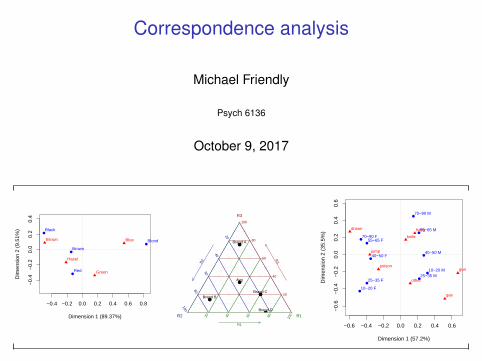
Correspondence analysis

Michael Friendly

Psych 6136

October 9, 2017

Dimension 1 (89.37%)

Dim

ensi

on 2

(9.

51%

)

−0.4 −0.2 0.0 0.2 0.4 0.6 0.8

−0.

4−

0.2

0.0

0.2

0.4

●

●

●

●

Black

Brown

Red

BlondBrown Blue

Hazel

Green

●

●

●

●

●

Brand A

Brand BBrand C

Brand D

Avg

20

40

60

80

100

20

40

60

80

100

20 40 60 80 100

R3R

2

R1

R3

R2 R1

Dimension 1 (57.2%)

Dim

ensi

on 2

(35

.5%

)−0.6 −0.4 −0.2 0.0 0.2 0.4 0.6

−0.

6−

0.4

−0.

20.

00.

20.

40.

6

●

●

●

●

●●

●

●

●

●

10−20 F

10−20 M

25−35 F25−35 M

40−50 F40−50 M

55−65 F

55−65 M

70−90 F

70−90 M

poison

gas

hangdrown

gun

knife

jump

other

Basic ideas

Correspondence analysis: Basic ideas

Correspondence analysis (CA)

Analog of PCA for frequency data:account for maximum % of χ2 in few (2-3) dimensionsfinds scores for row (xim) and column (yjm) categories on thesedimensionsuses Singular Value Decomposition of residuals from independence,

dij = (nij − m̂ij )/√

m̂ij

dij =√

nM∑

m=1

λm xim yjm ↔ D = XΛY T

optimal scaling: each pair of scores for rows (xim) and columns (yjm) havehighest possible correlation (= λm).plots of the row (xim) and column (yjm) scores show associations

2 / 1

Basic ideas

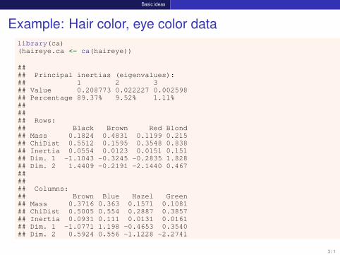
Example: Hair color, eye color datalibrary(ca)(haireye.ca <- ca(haireye))

#### Principal inertias (eigenvalues):## 1 2 3## Value 0.208773 0.022227 0.002598## Percentage 89.37% 9.52% 1.11%###### Rows:## Black Brown Red Blond## Mass 0.1824 0.4831 0.1199 0.215## ChiDist 0.5512 0.1595 0.3548 0.838## Inertia 0.0554 0.0123 0.0151 0.151## Dim. 1 -1.1043 -0.3245 -0.2835 1.828## Dim. 2 1.4409 -0.2191 -2.1440 0.467###### Columns:## Brown Blue Hazel Green## Mass 0.3716 0.363 0.1571 0.1081## ChiDist 0.5005 0.554 0.2887 0.3857## Inertia 0.0931 0.111 0.0131 0.0161## Dim. 1 -1.0771 1.198 -0.4653 0.3540## Dim. 2 0.5924 0.556 -1.1228 -2.2741

3 / 1

Basic ideas

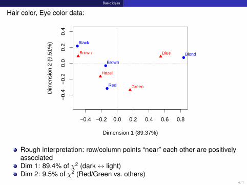
Hair color, Eye color data:


Dim

ensi

on 2

(9.

51%

)

−0.4 −0.2 0.0 0.2 0.4 0.6 0.8

−0.

4−

0.2

0.0

0.2

0.4

●

●

●

●

Black

Brown

Red

BlondBrown Blue

Hazel

Green

Rough interpretation: row/column points “near” each other are positivelyassociatedDim 1: 89.4% of χ2 (dark↔ light)Dim 2: 9.5% of χ2 (Red/Green vs. others)

4 / 1

Basic ideas

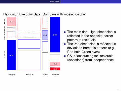
Hair color, Eye color data: Compare with mosaic display

4.4

-3.1

2.3

-5.9

-2.2

7.0

Black Brown Red Blond

Bro

wn

Ha

ze

l G

ree

n

Blu

e

The main dark–light dimension isreflected in the opposite-cornerpattern of residualsThe 2nd dimension is reflected indeviations from this pattern (e.g.,Red hair–Green eyes)CA is “accounting for” residuals(deviations) from independence

5 / 1

Basic ideas Profiles

Row and column profiles

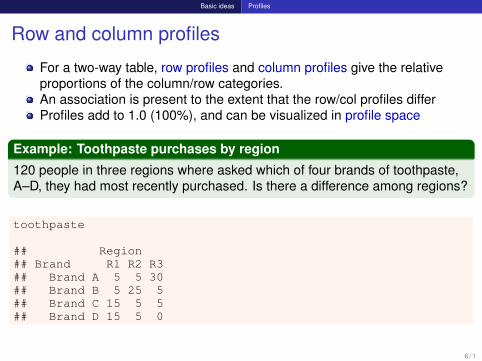
For a two-way table, row profiles and column profiles give the relativeproportions of the column/row categories.An association is present to the extent that the row/col profiles differProfiles add to 1.0 (100%), and can be visualized in profile space

Example: Toothpaste purchases by region

120 people in three regions where asked which of four brands of toothpaste,A–D, they had most recently purchased. Is there a difference among regions?

toothpaste

## Region## Brand R1 R2 R3## Brand A 5 5 30## Brand B 5 25 5## Brand C 15 5 5## Brand D 15 5 0

6 / 1


Row and column profiles

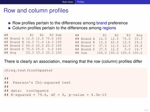
Row profiles pertain to the differences among brand preferenceColumn profiles pertain to the differences among regions

## R1 R2 R3 Sum## Brand A 12.5 12.5 75.0 100## Brand B 14.3 71.4 14.3 100## Brand C 60.0 20.0 20.0 100## Brand D 75.0 25.0 0.0 100## Avg 33.3 33.3 33.3 100

## R1 R2 R3 Avg## Brand A 12.5 12.5 75.0 33.3## Brand B 12.5 62.5 12.5 29.2## Brand C 37.5 12.5 12.5 20.8## Brand D 37.5 12.5 0.0 16.7## Sum 100.0 100.0 100.0 100.0

There is clearly an association, meaning that the row (column) profiles differ

chisq.test(toothpaste)

#### Pearson's Chi-squared test#### data: toothpaste## X-squared = 79.6, df = 6, p-value = 4.3e-15

7 / 1


Plotting profiles

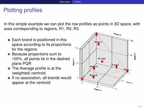
In this simple example we can plot the row profiles as points in 3D space, withaxes corresponding to regions, R1, R2, R3

Each brand is positioned in thisspace according to its proportionsfor the regionsBecause proportions sum to100%, all points lie in the dashedplane PQRThe Average profile is at the(weighted) centroidIf no association, all brands wouldappear at the centroid

8 / 1


Plotting profiles

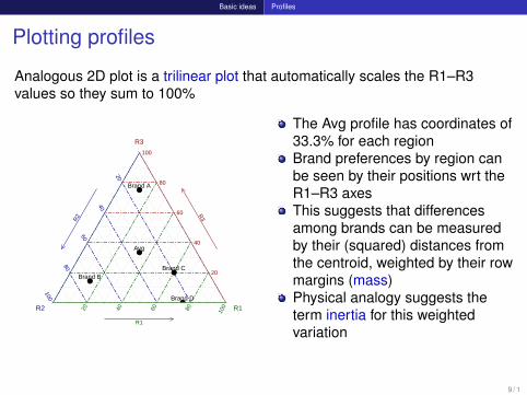
Analogous 2D plot is a trilinear plot that automatically scales the R1–R3values so they sum to 100%

●

●

●

●

●

Brand A

Brand BBrand C

Brand D

Avg

20

40

60

80

100

20

40

60

80

100

20 40 60 80 100

R3R

2

R1

R3

R2 R1

The Avg profile has coordinates of33.3% for each regionBrand preferences by region canbe seen by their positions wrt theR1–R3 axesThis suggests that differencesamong brands can be measuredby their (squared) distances fromthe centroid, weighted by their rowmargins (mass)Physical analogy suggests theterm inertia for this weightedvariation

9 / 1


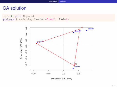
CA solutionThe CA solution has at most min(r − 1, c − 1) dimensionsA 2D solution here is exact, i.e., accounts for 100% of Pearson X 2

library(ca)tp.ca <- ca(toothpaste)summary(tp.ca, rows=FALSE, columns=FALSE)

#### Principal inertias (eigenvalues):#### dim value % cum% scree plot## 1 0.410259 61.8 61.8 ***************## 2 0.253134 38.2 100.0 **********## -------- -----## Total: 0.663393 100.0

Pearson X 2:

sum(tp.ca$svˆ2) * 120

## [1] 79.607

10 / 1


CA solution

res <- plot(tp.ca)polygon(res$cols, border="red", lwd=2)


Dim

ensi

on 2

(38

.16%

)

−1.0 −0.5 0.0 0.5

−0.

6−

0.4

−0.

20.

00.

20.

40.

6

●

●

●

●

BrandA

BrandB

BrandCBrandD

R1

R2

R3

11 / 1


12 / 1

Basic ideas SVD

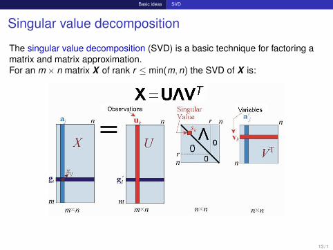
Singular value decomposition

The singular value decomposition (SVD) is a basic technique for factoring amatrix and matrix approximation.For an m × n matrix X of rank r ≤ min(m,n) the SVD of X is:

13 / 1

Basic ideas SVD

Properties of the SVD

14 / 1

Basic ideas SVD

SVD: Matrix approximation

15 / 1

Basic ideas CA coordinates

CA notation and terminology

Notation:Contingency table: N = {nij}Correspondence matrix (cell probabilities): P = {pij} = N/nRow/column masses (marginal probabilities): r =

∑j pij and c =

∑i pij

Diagonal weight matrices: Dr = diag (r) and Dc = diag (c)

The SVD is then applied to the correspondence matrix of cell probabilities as:

P = ADλBT

whereSingular values: Dλ = diag (λ) is the diagonal matrix of singular valuesλ1 ≥ λ2 ≥ · · · ≥ λMRow scores: AI×M , normalized so that AD−1

r AT = IColumn scores: BJ×M , normalized so that BD−1

c BT = I

16 / 1


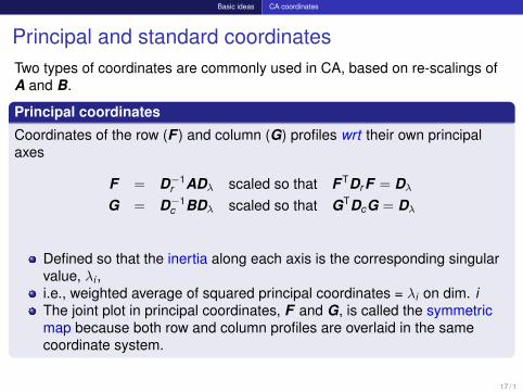
Principal and standard coordinatesTwo types of coordinates are commonly used in CA, based on re-scalings ofA and B.

Principal coordinates

Coordinates of the row (F ) and column (G) profiles wrt their own principalaxes

F = D−1r ADλ scaled so that F TDr F = Dλ

G = D−1c BDλ scaled so that GTDcG = Dλ

Defined so that the inertia along each axis is the corresponding singularvalue, λi ,i.e., weighted average of squared principal coordinates = λi on dim. iThe joint plot in principal coordinates, F and G, is called the symmetricmap because both row and column profiles are overlaid in the samecoordinate system.

17 / 1


Principal and standard coordinates

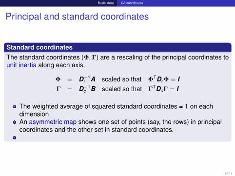
Standard coordinatesThe standard coordinates (Φ,Γ) are a rescaling of the principal coordinates tounit inertia along each axis,

Φ = D−1r A scaled so that ΦTDrΦ = I

Γ = D−1c B scaled so that ΓTDcΓ = I

The weighted average of squared standard coordinates = 1 on eachdimensionAn asymmetric map shows one set of points (say, the rows) in principalcoordinates and the other set in standard coordinates.

18 / 1


Geometric and statistical properties

nested solutions: CA solutions are nested , meaning that the first twodimensions of a 3D solution will be identical to the 2D solution(similar to PCA)

centroids at the origin: In both principal coordinates and standard coordinatesthe points representing the row and column profiles have theircentroids (weighted averages) at the origin. The originrepresents the (weighted) average row profile and columnprofile.

chi-square distances: In principal coordinates, the row coordinates are equalto the row profiles D−1

r P, rescaled inversely by the square-rootof the column masses, D−1/2

c . Distances between two rowprofiles, Ri and Ri′ are χ2 distances, where the squareddifference [Rij − Ri′ j ]

2 is inversely weighted by the columnfrequency, to account for the different relative frequency of thecolumn categories.

19 / 1

Basic ideas ca package

The ca package in R

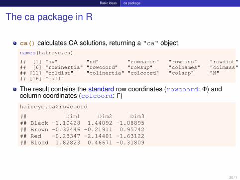
ca() calculates CA solutions, returning a "ca" objectnames(haireye.ca)

## [1] "sv" "nd" "rownames" "rowmass" "rowdist"## [6] "rowinertia" "rowcoord" "rowsup" "colnames" "colmass"## [11] "coldist" "colinertia" "colcoord" "colsup" "N"## [16] "call"

The result contains the standard row coordinates (rowcoord: Φ) andcolumn coordinates (colcoord: Γ)

haireye.ca$rowcoord

## Dim1 Dim2 Dim3## Black -1.10428 1.44092 -1.08895## Brown -0.32446 -0.21911 0.95742## Red -0.28347 -2.14401 -1.63122## Blond 1.82823 0.46671 -0.31809

20 / 1


The ca package in R

The plot() method provides a wide variety of scalings (map=), with differentinterpretive properties. Some of these are:

"symmetric" — both rows and columns in pricipal coordinates (default)"rowprincipal" or "colprincipal" — asymmetric maps, witheither rows in principal coordinates and columns in standard coordinates,or vice versa"symbiplot" — scales both rows and columns to have variances equalto the singular value

The mcja() function is used for multiple correspondence analysis (MCA) andhas analogous print(), summary() and plot() methods.

21 / 1


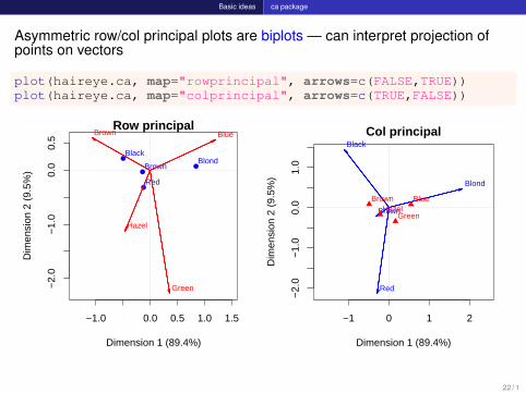
Asymmetric row/col principal plots are biplots — can interpret projection ofpoints on vectors

plot(haireye.ca, map="rowprincipal", arrows=c(FALSE,TRUE))plot(haireye.ca, map="colprincipal", arrows=c(TRUE,FALSE))

Dimension 1 (89.4%)

Dim

ensi

on 2

(9.

5%)

−1.0 0.0 0.5 1.0 1.5

−2.

0−

1.0

0.0

0.5

●

●

●

●

Black

Brown

Red

Blond

Brown Blue

Hazel

Green

Row principal

Dimension 1 (89.4%)

Dim

ensi

on 2

(9.

5%)

−1 0 1 2

−2.

0−

1.0

0.0

1.0

Black

Brown

Red

Blond

Brown BlueHazel

Green

Col principal

22 / 1

Basic ideas CA properties

Optimal category scores

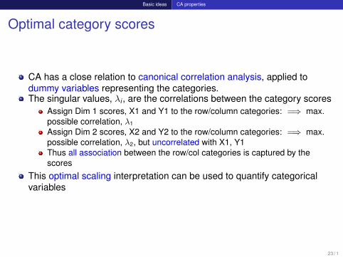
CA has a close relation to canonical correlation analysis, applied todummy variables representing the categories.The singular values, λi , are the correlations between the category scores

Assign Dim 1 scores, X1 and Y1 to the row/column categories: =⇒ max.possible correlation, λ1

Assign Dim 2 scores, X2 and Y2 to the row/column categories: =⇒ max.possible correlation, λ2, but uncorrelated with X1, Y1Thus all association between the row/col categories is captured by thescores

This optimal scaling interpretation can be used to quantify categoricalvariables

23 / 1


Optimal category scores

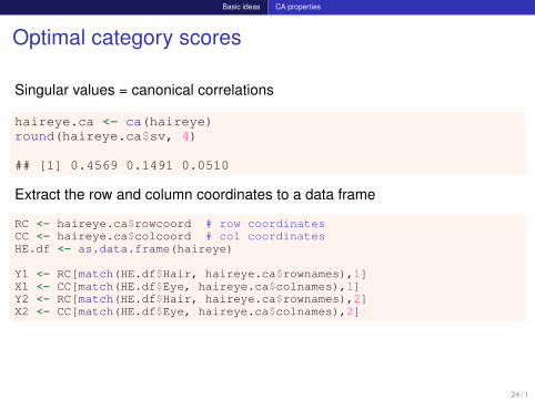
Singular values = canonical correlations

haireye.ca <- ca(haireye)round(haireye.ca$sv, 4)

## [1] 0.4569 0.1491 0.0510

Extract the row and column coordinates to a data frame

RC <- haireye.ca$rowcoord # row coordinatesCC <- haireye.ca$colcoord # col coordinatesHE.df <- as.data.frame(haireye)

Y1 <- RC[match(HE.df$Hair, haireye.ca$rownames),1]X1 <- CC[match(HE.df$Eye, haireye.ca$colnames),1]Y2 <- RC[match(HE.df$Hair, haireye.ca$rownames),2]X2 <- CC[match(HE.df$Eye, haireye.ca$colnames),2]

24 / 1


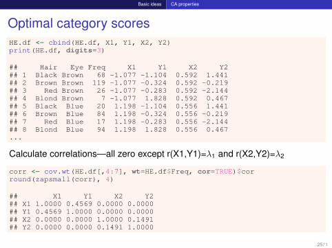
Optimal category scoresHE.df <- cbind(HE.df, X1, Y1, X2, Y2)print(HE.df, digits=3)

## Hair Eye Freq X1 Y1 X2 Y2## 1 Black Brown 68 -1.077 -1.104 0.592 1.441## 2 Brown Brown 119 -1.077 -0.324 0.592 -0.219## 3 Red Brown 26 -1.077 -0.283 0.592 -2.144## 4 Blond Brown 7 -1.077 1.828 0.592 0.467## 5 Black Blue 20 1.198 -1.104 0.556 1.441## 6 Brown Blue 84 1.198 -0.324 0.556 -0.219## 7 Red Blue 17 1.198 -0.283 0.556 -2.144## 8 Blond Blue 94 1.198 1.828 0.556 0.467...

Calculate correlations—all zero except r(X1,Y1)=λ1 and r(X2,Y2)=λ2

corr <- cov.wt(HE.df[,4:7], wt=HE.df$Freq, cor=TRUE)$corround(zapsmall(corr), 4)

## X1 Y1 X2 Y2## X1 1.0000 0.4569 0.0000 0.0000## Y1 0.4569 1.0000 0.0000 0.0000## X2 0.0000 0.0000 1.0000 0.1491## Y2 0.0000 0.0000 0.1491 1.0000

25 / 1


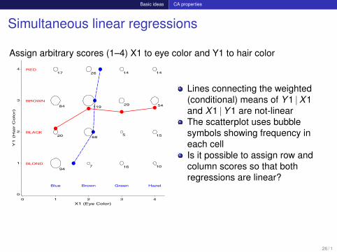
Simultaneous linear regressions

Assign arbitrary scores (1–4) X1 to eye color and Y1 to hair color

BLACK

BLOND

BROWN

RED

Blue Brown Green Hazel

’

Y1

(H

air C

olo

r)

0

1

2

3

4

X1 (Eye Color)0 1 2 3 4

20

94

84

17

68

7

119

26

5

16

29

14

15

10

54

14

Lines connecting the weighted(conditional) means of Y 1 |X1and X1 |Y 1 are not-linearThe scatterplot uses bubblesymbols showing frequency ineach cellIs it possible to assign row andcolumn scores so that bothregressions are linear?

26 / 1


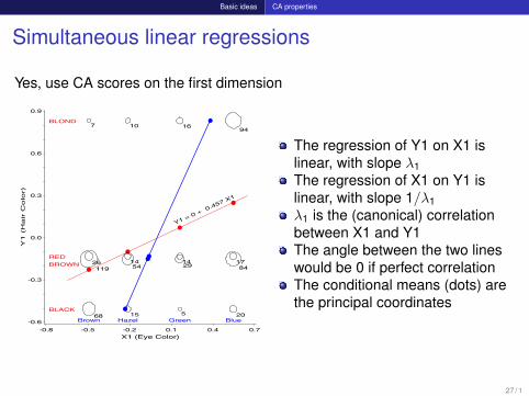
Simultaneous linear regressions

Yes, use CA scores on the first dimension

BLACK

BROWN

RED

BLOND

Brown BlueHazel Green

Y1 = 0 + 0.457 X

1

’

Y1 (

Hair C

olo

r)

-0.6

-0.3

0.0

0.3

0.6

0.9

X1 (Eye Color)-0.8 -0.5 -0.2 0.1 0.4 0.7

68

11926

7

20

8417

94

15

5414

10

5

2914

16

The regression of Y1 on X1 islinear, with slope λ1The regression of X1 on Y1 islinear, with slope 1/λ1λ1 is the (canonical) correlationbetween X1 and Y1The angle between the two lineswould be 0 if perfect correlationThe conditional means (dots) arethe principal coordinates

27 / 1

CA examples

Example: Mental impairment and parents’ SES

Data on mental health status (mental) of 1660 young NYC residents byparents’ SES (ses), a 6× 4 table.

Both mental and ses are ordered factorsConvert from frequency data frame to table using xtabs()

data("Mental", package="vcdExtra")str(Mental)

## 'data.frame': 24 obs. of 3 variables:## $ ses : Ord.factor w/ 6 levels "1"<"2"<"3"<"4"<..: 1 1 1 1 2 2 2 2 3 3 ...## $ mental: Ord.factor w/ 4 levels "Well"<"Mild"<..: 1 2 3 4 1 2 3 4 1 2 ...## $ Freq : int 64 94 58 46 57 94 54 40 57 105 ...

mental.tab <- xtabs(Freq ˜ ses + mental, data=Mental)

28 / 1

CA examples

Example: Mental impairment and parents’ SES

mental.ca <- ca(mental.tab)summary(mental.ca)

#### Principal inertias (eigenvalues):#### dim value % cum% scree plot## 1 0.026025 93.9 93.9 ***********************## 2 0.001379 5.0 98.9 *## 3 0.000298 1.1 100.0## -------- -----## Total: 0.027702 100.0...

The exact CA solution has min(r − 1, c − 1) = 3 dimensionsThe total Pearson X 2 is nΣλ2

i = 1660× 0.0277 = 45.98 with 15 dfOf this, 93.9% is accounted for by the first dimension

29 / 1

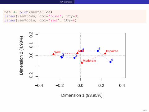
CA examples

res <- plot(mental.ca)lines(res$rows, col="blue", lty=3)lines(res$cols, col="red", lty=4)


Dim

ensi

on 2

(4.

98%

)

−0.4 −0.2 0.0 0.2 0.4

−0.

20.

00.

10.

2

●● ●

● ●

●

12 3

4 5

6

Well Mild

Moderate

Impaired

30 / 1

CA examples

Looking ahead

CA is largely an exploratory method — row/column scores are notparameters of a statistical model; no confidence intervalsOnly rough tests for the number of CA dimensionsCan’t test an hypothesis that the row/column scores are have someparticular spacing (e.g., are mental and ses equally spaced?)These kinds of questions can be answered with specialized loglinearmodelsNevertheless, plot(ca(table)) gives an excellent quick view ofassociations

31 / 1

Multi-way tables

Multi-way tables

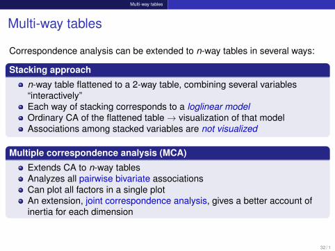
Correspondence analysis can be extended to n-way tables in several ways:

Stacking approach

n-way table flattened to a 2-way table, combining several variables“interactively”Each way of stacking corresponds to a loglinear modelOrdinary CA of the flattened table→ visualization of that modelAssociations among stacked variables are not visualized

Multiple correspondence analysis (MCA)

Extends CA to n-way tablesAnalyzes all pairwise bivariate associationsCan plot all factors in a single plotAn extension, joint correspondence analysis, gives a better account ofinertia for each dimension

32 / 1

Multi-way tables Stacking

Multi-way tables: Stacking

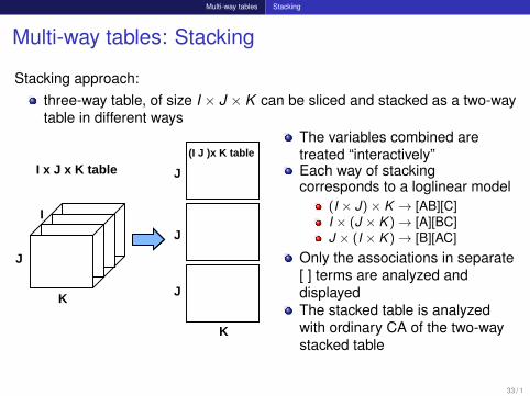
Stacking approach:three-way table, of size I × J × K can be sliced and stacked as a two-waytable in different ways

K

J

I

I x J x K table

K

J

J

J

(I J )x K tableThe variables combined aretreated “interactively”Each way of stackingcorresponds to a loglinear model

(I × J)× K → [AB][C]I × (J × K )→ [A][BC]J × (I × K )→ [B][AC]

Only the associations in separate[ ] terms are analyzed anddisplayedThe stacked table is analyzedwith ordinary CA of the two-waystacked table

33 / 1


Interactive coding in R

Data in table (array) form: Use as.matrix(structable())

mat1 <- as.matrix(structable(A + B ˜ C, data=mytable)) # [A B][C]mat2 <- as.matrix(structable(A + C ˜ B + D, data=mytable)) # [A C][B D]ca(mat2)

Data in frequency data frame form: Use paste() or interaction(),followed by xtabs()mydf$AB <- interaction(mydf$A, mydf$B, sep='.') # levels: A.Bmydf$AB <- paste(mydf$A, mydf$B, sep=':') # levels: A:B...mytab <- xtabs(Freq ˜ AB + C, data=mydf) # [A B] [C}

34 / 1


Example: Suicide rates in Germany

Suicide in vcd gives a 2× 5× 8 table of sex by age.group by methodof suicide for 53,182 suicides in Germany, in a frequency data frameWith the data in this form, you can use paste() to join age.group andsex together to form a new variable age_sex consisting of theircombinations.

data("Suicide", package="vcd")# interactive coding of sex and age.groupSuicide <- within(Suicide, {

age_sex <- paste(age.group, toupper(substr(sex,1,1)))})

35 / 1



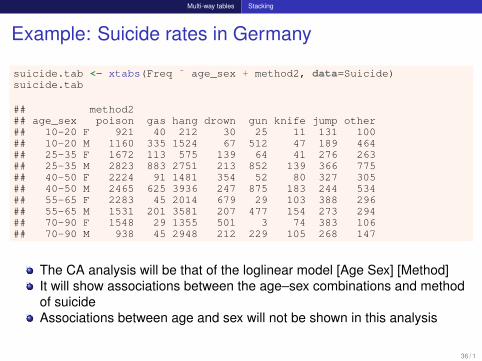
suicide.tab <- xtabs(Freq ˜ age_sex + method2, data=Suicide)suicide.tab

## method2## age_sex poison gas hang drown gun knife jump other## 10-20 F 921 40 212 30 25 11 131 100## 10-20 M 1160 335 1524 67 512 47 189 464## 25-35 F 1672 113 575 139 64 41 276 263## 25-35 M 2823 883 2751 213 852 139 366 775## 40-50 F 2224 91 1481 354 52 80 327 305## 40-50 M 2465 625 3936 247 875 183 244 534## 55-65 F 2283 45 2014 679 29 103 388 296## 55-65 M 1531 201 3581 207 477 154 273 294## 70-90 F 1548 29 1355 501 3 74 383 106## 70-90 M 938 45 2948 212 229 105 268 147

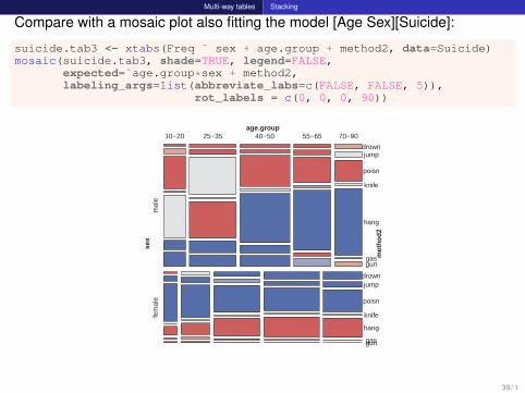
The CA analysis will be that of the loglinear model [Age Sex] [Method]It will show associations between the age–sex combinations and methodof suicideAssociations between age and sex will not be shown in this analysis

36 / 1



suicide.ca <- ca(suicide.tab)summary(suicide.ca)

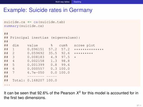
#### Principal inertias (eigenvalues):#### dim value % cum% scree plot## 1 0.096151 57.2 57.2 **************## 2 0.059692 35.5 92.6 *********## 3 0.008183 4.9 97.5 *## 4 0.002158 1.3 98.8## 5 0.001399 0.8 99.6## 6 0.000557 0.3 100.0## 7 6.7e-050 0.0 100.0## -------- -----## Total: 0.168207 100.0...

It can be seen that 92.6% of the Pearson X 2 for this model is accounted for inthe first two dimensions.

37 / 1


plot(suicide.ca)

Dimension 1 (57.2%)

Dim

ensi

on 2

(35

.5%

)

−0.6 −0.4 −0.2 0.0 0.2 0.4 0.6

−0.

6−

0.4

−0.

20.

00.

20.

40.

6

●

●

●

●

●●

●

●

●

●

10−20 F

10−20 M

25−35 F25−35 M

40−50 F40−50 M

55−65 F

55−65 M

70−90 F

70−90 M

poison

gas

hangdrown

gun

knife

jump

other

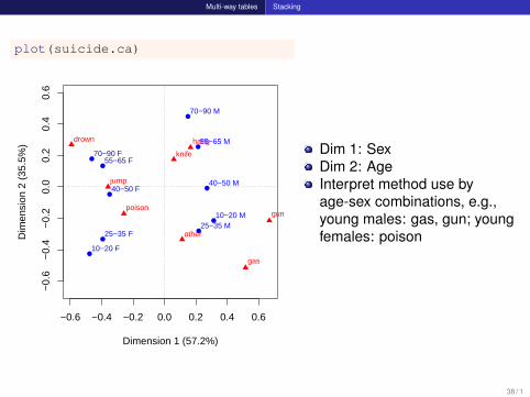
Dim 1: SexDim 2: AgeInterpret method use byage-sex combinations, e.g.,young males: gas, gun; youngfemales: poison

38 / 1


Compare with a mosaic plot also fitting the model [Age Sex][Suicide]:

suicide.tab3 <- xtabs(Freq ˜ sex + age.group + method2, data=Suicide)mosaic(suicide.tab3, shade=TRUE, legend=FALSE,

expected=˜age.group*sex + method2,labeling_args=list(abbreviate_labs=c(FALSE, FALSE, 5)),

rot_labels = c(0, 0, 0, 90))

age.group

sex

met

hod2

fem

ale

gungas

hang

knife

poisn

jumpdrown

mal

e

10−20 25−35 40−50 55−65 70−90

gungas

hang

knife

poisn

jumpdrown

39 / 1

Multi-way tables Marginal tables

Marginal tables and supplementary variablesAn n-way table is collapsed to a marginal table by ignoring factorsOmitted variables can be included by treating them as supplementaryThese are projected into the space of the marginal CA

Age by method, ignoring sex:suicide.tab2 <- xtabs(Freq ˜ age.group + method2, data=Suicide)suicide.tab2

## method2## age.group poison gas hang drown gun knife jump other## 10-20 2081 375 1736 97 537 58 320 564## 25-35 4495 996 3326 352 916 180 642 1038## 40-50 4689 716 5417 601 927 263 571 839## 55-65 3814 246 5595 886 506 257 661 590## 70-90 2486 74 4303 713 232 179 651 253

Relation of sex and method:(suicide.sup <- xtabs(Freq ˜ sex + method2, data=Suicide))

## method2## sex poison gas hang drown gun knife jump other## male 8917 2089 14740 946 2945 628 1340 2214## female 8648 318 5637 1703 173 309 1505 1070

suicide.tab2s <- rbind(suicide.tab2, suicide.sup)40 / 1


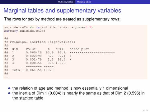
Marginal tables and supplementary variablesThe rows for sex by method are treated as supplementary rows:

suicide.ca2s <- ca(suicide.tab2s, suprow=6:7)summary(suicide.ca2s)

#### Principal inertias (eigenvalues):#### dim value % cum% scree plot## 1 0.060429 93.9 93.9 ***********************## 2 0.002090 3.2 97.1 *## 3 0.001479 2.3 99.4 *## 4 0.000356 0.6 100.0## -------- -----## Total: 0.064354 100.0##...

the relation of age and method is now essentially 1 dimensionalthe inertia of Dim 1 (0.604) is nearly the same as that of Dim 2 (0.596) inthe stacked table

41 / 1


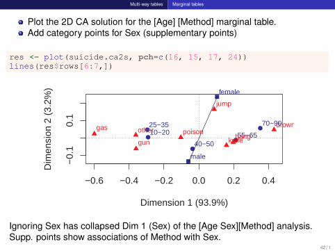
Plot the 2D CA solution for the [Age] [Method] marginal table.Add category points for Sex (supplementary points)

res <- plot(suicide.ca2s, pch=c(16, 15, 17, 24))lines(res$rows[6:7,])

Dimension 1 (93.9%)

Dim

ensi

on 2

(3.

2%)

−0.6 −0.4 −0.2 0.0 0.2 0.4

−0.

10.

1

●

●

●

●

●10−2025−35

40−5055−65

70−90

male

female

poisongas

hang

drown

gun knife

jump

other

Ignoring Sex has collapsed Dim 1 (Sex) of the [Age Sex][Method] analysis.Supp. points show associations of Method with Sex.

42 / 1

Multiple correspondence analysis

Multiple correspondence analysis (MCA)

Extends CA to n-way tablesUseful when simpler stacking approach doesn’t work well, e.g., 10categorical attitude itemsAnalyzes all pairwise bivariate associations. Analogous to:

Correlation matrix (numbers)Scatterplot matrix (graphs)All pairwise χ2 tests (numbers)Mosaic matrix (graphs)

Provides an optimal scaling of the category scores for each variableCan plot all factors in a single plotAn extension, joint correspondence analysis, gives a better account ofinertia for each dimension

43 / 1

Multiple correspondence analysis

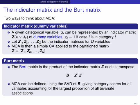
The indicator matrix and the Burt matrixTwo ways to think about MCA:

Indicator matrix (dummy variables)

A given categorical variable, q, can be represented by an indicator matrixZ (n × Jq) of dummy variables, zij = 1 if case i is in category jLet Z1,Z2, . . . ,ZQ be the indicator matrices for Q variablesMCA is then a simple CA applied to the partitioned matrixZ = [Z 1,Z2, . . . ,ZQ]

Burt matrixThe Bert matrix is the product of the indicator matrix Z and its transpose

B = Z TZ

MCA can be defined using the SVD of B, giving category scores for allvariables accounting for the largest proportion of all bivariateassociations.

44 / 1

Multiple correspondence analysis Bivariate MCA

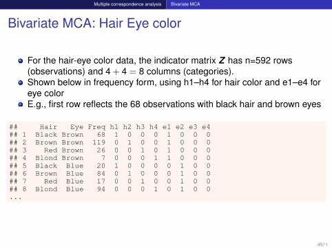
Bivariate MCA: Hair Eye color

For the hair-eye color data, the indicator matrix Z has n=592 rows(observations) and 4 + 4 = 8 columns (categories).Shown below in frequency form, using h1–h4 for hair color and e1–e4 foreye colorE.g., first row reflects the 68 observations with black hair and brown eyes

## Hair Eye Freq h1 h2 h3 h4 e1 e2 e3 e4## 1 Black Brown 68 1 0 0 0 1 0 0 0## 2 Brown Brown 119 0 1 0 0 1 0 0 0## 3 Red Brown 26 0 0 1 0 1 0 0 0## 4 Blond Brown 7 0 0 0 1 1 0 0 0## 5 Black Blue 20 1 0 0 0 0 1 0 0## 6 Brown Blue 84 0 1 0 0 0 1 0 0## 7 Red Blue 17 0 0 1 0 0 1 0 0## 8 Blond Blue 94 0 0 0 1 0 1 0 0...

45 / 1


Expand this to case form for Z (592 x 8)

Z <- expand.dft(haireye.df)[,-(1:2)]vnames <- c(levels(haireye.df$Hair), levels(haireye.df$Eye))colnames(Z) <- vnamesdim(Z)

## [1] 592 8

If the indicator matrix is partitioned as Z = [Z1,Z2], corresponding to the hair,eye categories, then the contingency table is given by N = Z T

1 Z2.

(N <- t(as.matrix(Z[,1:4])) %*% as.matrix(Z[,5:8]))

## Brown Blue Hazel Green## Black 68 20 15 5## Brown 119 84 54 29## Red 26 17 14 14## Blond 7 94 10 16

46 / 1


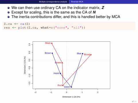
We can then use ordinary CA on the indicator matrix, ZExcept for scaling, this is the same as the CA of NThe inertia contributions differ, and this is handled better by MCA

Z.ca <- ca(Z)res <- plot(Z.ca, what=c("none", "all"))

Dimension 1 (24.3%)

Dim

ensi

on 2

(19

.2%

)

−2 −1 0 1 2

−1.

5−

1.0

−0.

50.

00.

51.

0

Brown

Hazel

Green

Blue

Black

Brown

Red

Blond●

●

●

●

47 / 1


The Burt matrixFor two categorical variables, the Burt matrix is

B = Z TZ =

[N1 NNT N2

].

N1 and N2 are diagonal matrices containing the marginal frequencies ofthe two variablesThe contingency table, N appears in the off-diagonal block

A similar analysis to that of the indicator matrix Z is produced by:

Burt <- t(as.matrix(Z)) %*% as.matrix(Z)rownames(Burt) <- colnames(Burt) <- vnamesBurt.ca <- ca(Burt)plot(Burt.ca)

Standard coords are the sameSingular values of B are the squares of those of Z

48 / 1

Multiple correspondence analysis Multivariate MCA

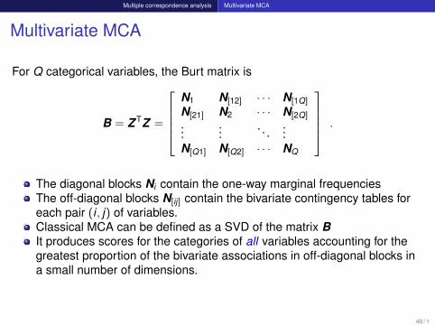
Multivariate MCA

For Q categorical variables, the Burt matrix is

B = Z TZ =

N1 N[12] · · · N[1Q]

N[21] N2 · · · N[2Q]

......

. . ....

N[Q1] N[Q2] · · · NQ

.

The diagonal blocks Ni contain the one-way marginal frequenciesThe off-diagonal blocks N[ij] contain the bivariate contingency tables foreach pair (i , j) of variables.Classical MCA can be defined as a SVD of the matrix BIt produces scores for the categories of all variables accounting for thegreatest proportion of the bivariate associations in off-diagonal blocks ina small number of dimensions.

49 / 1

Multiple correspondence analysis Multivariate MCA

MCA properties

The inertia contributed by a given variable increases with the number ofresponse categories: inertia (Zq) = Jq − 1The centroid of the categories for each variable is at the origin of thedisplay.For a given variable, the inertia contributed by a given category increasesas the marginal frequency in that category decreases. Low frequencypoints therefore appear further from the origin.The category points for a binary variable lie on a line through the origin.

50 / 1

Multiple correspondence analysis MCA example

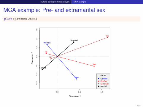
MCA example: Pre- and extramarital sex

PreSex data: the 2× 2× 2× 2 table of gender, premarital sex,extramatrial sex and marital status (divorced, still married)The function mjca() provides several scalings for the singular valuesHere I use lambda="Burt"

data("PreSex", package="vcd")PreSex <- aperm(PreSex, 4:1) # order variables G, P, E, Mpresex.mca <- mjca(PreSex, lambda="Burt")summary(presex.mca)

#### Principal inertias (eigenvalues):#### dim value % cum% scree plot## 1 0.149930 53.6 53.6 *************## 2 0.067201 24.0 77.6 ******## 3 0.035396 12.6 90.2 ***## 4 0.027365 9.8 100.0 **## -------- -----## Total: 0.279892 100.0...

51 / 1

Multiple correspondence analysis MCA example

MCA example: Pre- and extramarital sexplot(presex.mca)

Dimension 1

Dim

ensi

on 2

0.0 0.5 1.0

−0.

6−

0.4

−0.

20.

00.

20.

40.

6

●

●

●

●

Men

Women

No

Yes

No

Yes

Divorced

Married

●

●

Factor

GenderPreSexExtraSexMarital

52 / 1

Multiple correspondence analysis MCA inertia

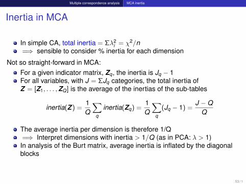
Inertia in MCA

In simple CA, total inertia = Σλ2i = χ2/n

=⇒ sensible to consider % inertia for each dimension

Not so straight-forward in MCA:For a given indicator matrix, Zq , the inertia is Jq − 1For all variables, with J = ΣJq categories, the total inertia ofZ = [Z1, . . . ,ZQ] is the average of the inertias of the sub-tables

inertia(Z ) =1Q

∑q

inertia(Zq) =1Q

∑q

(Jq − 1) =J −Q

Q

The average inertia per dimension is therefore 1/Q=⇒ Interpret dimensions with inertia > 1/Q (as in PCA: λ > 1)In analysis of the Burt matrix, average inertia is inflated by the diagonalblocks

53 / 1


Inertia in MCA

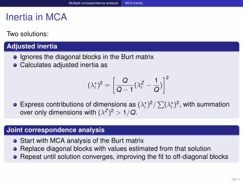
Two solutions:

Adjusted inertia

Ignores the diagonal blocks in the Burt matrixCalculates adjusted inertia as

(λ?i )2 =

[Q

Q − 1(λZ

i −1Q

)

]2

Express contributions of dimensions as (λ?i )2/∑

(λ?i )2, with summationover only dimensions with (λZ )2 > 1/Q.

Joint correspondence analysis

Start with MCA analysis of the Burt matrixReplace diagonal blocks with values estimated from that solutionRepeat until solution converges, improving the fit to off-diagonal blocks

54 / 1


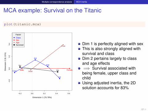
MCA example: Survival on the Titanic

Analyze the Titanic data, using mjca()The default inertia method is lambda="adjusted"Other methods are "indicator", "Burt", "JCA"

data(Titanic)titanic.mca <- mjca(Titanic)summary(titanic.mca)

#### Principal inertias (eigenvalues):#### dim value % cum% scree plot## 1 0.067655 76.8 76.8 ***********************## 2 0.005386 6.1 82.9 **## 3 00000000 0.0 82.9## -------- -----## Total: 0.088118...

55 / 1


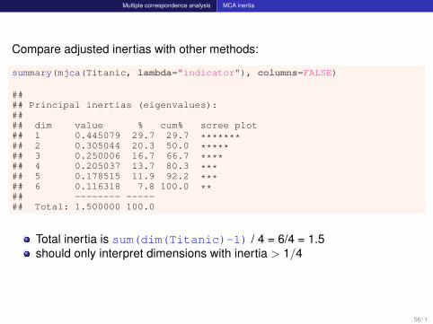
Compare adjusted inertias with other methods:

summary(mjca(Titanic, lambda="indicator"), columns=FALSE)

#### Principal inertias (eigenvalues):#### dim value % cum% scree plot## 1 0.445079 29.7 29.7 *******## 2 0.305044 20.3 50.0 *****## 3 0.250006 16.7 66.7 ****## 4 0.205037 13.7 80.3 ***## 5 0.178515 11.9 92.2 ***## 6 0.116318 7.8 100.0 **## -------- -----## Total: 1.500000 100.0

Total inertia is sum(dim(Titanic)-1) / 4 = 6/4 = 1.5should only interpret dimensions with inertia > 1/4

56 / 1


MCA example: Survival on the Titanic

plot(titanic.mca)


Dim

ensi

on 2

(6.

11%

)

−0.2 0.0 0.2 0.4 0.6

−0.

20.

00.

20.

4

●

●

●

●

●

●

1st

2nd

3rd

Crew FemaleMaleAdult

Child

No

Yes

●

●

Factor

ClassSexAgeSurvived Dim 1 is perfectly aligned with sex

This is also strongly aligned withsurvival and classDim 2 pertains largely to classand age effects=⇒ Survival associated withbeing female, upper class andchildUsing adjusted inertia, the 2Dsolution accounts for 83%

57 / 1

Biplots

Biplots for contingency tables

The biplot is another visualization method that also uses the SVD to give alow-rank (2D) representation.

In CA, the (weighted) χ2 distances between row (column) points reflectthe differences among row (column) profilesIn the biplot, rows and columns are represented by vectors from theorigin with an inner product (projection) interpretation

Y ≈ ABT ⇐⇒ yij ≈ aTi bj

||a|| cos θ

a

bθ

||a||

58 / 1

Biplots

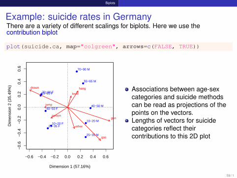
Example: suicide rates in GermanyThere are a variety of different scalings for biplots. Here we use thecontribution biplot

plot(suicide.ca, map="colgreen", arrows=c(FALSE, TRUE))


Dim

ensi

on 2

(35

.49%

)

−0.6 −0.4 −0.2 0.0 0.2 0.4 0.6

−0.

6−

0.4

−0.

20.

00.

20.

40.

6

●●

●

●

●●

●

●

●

●

10−20 F10−20 M

25−35 F

25−35 M

40−50 F40−50 M

55−65 F

55−65 M

70−90 F

70−90 M

poison

gas

hangdrown

gun

knife

jump

other

Associations between age-sexcategories and suicide methodscan be read as projections of thepoints on the vectors.Lengths of vectors for suicidecategories reflect theircontributions to this 2D plot

59 / 1

Summary

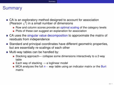
Summary

CA is an exploratory method designed to account for association(Pearson χ2) in a small number of dimensions

Row and column scores provide an optimal scaling of the category levelsPlots of these can suggest an explanation for association

CA uses the singular value decomposition to approximate the matrix ofresiduals from independenceStandard and principal coordinates have different geometric properties,but are essentially re-scalings of each otherMulti-way tables can be handled by:

Stacking approach— collapse some dimensions interactively to a 2-waytableEach way of stacking→ a loglinear modelMCA analyzes the full n− way table using an indicator matrix or the Burtmatrix

60 / 1

Documents

Correspondence analysis - York Universityeuclid.psych.yorku.ca/www/psy6136/lectures/Corresp-1up.pdf · Correspondence analysis: Basic ideas Correspondence analysis (CA) Analog of