Embed Size (px)
Citation preview
Note 12
WHEN YOUNG CANADIAN ADULTS
RETURN TO SCHOOL:
A DECISION ANCHORED IN THE INDIVIDUAL’S
SOCIAL AND ACADEMIC PAST
NOVEMBER 2010

Published in 2010 by the
Centre interuniversitaire de recherche
sur la science et la technologie (CIRST)
Université du Québec à Montréal (UQAM)
C.P. 8888, Succursale Centre-ville
Montréal (Québec)
Canada H3C 3P8
Web: http://www.cirst.uqam.ca
E-mail: [email protected]
With the financial support of
The Canada Millennium Scholarship Foundation
ISBN 978-2-923333-59-5
Legal Deposit: 2010
Bibliothèque et Archives nationales du Québec
Library and Archives Canada
Ce document est aussi disponible en français sous le titre :
Les retours aux études postsecondaires chez les jeunes adultes canadiens :
une décision fortement ancrée au passé social et scolaire de l’individu.
Translation: Daly-Dallaire
Layout : Edmond-Louis Dussault
Internet references have been verified at time of publication.
The opinions expressed in this research document are those of the authors and do not represent
official policies of the Canada Millennium Scholarship Foundation and other agencies or
organizations that may have provided support, financial or otherwise, for this project.
Research Note 12
When Young Canadian Adults
Return to School:
A Decision Anchored in the Individual’s
Social and Academic Past
Benoît Laplante
María Constanza Street
Pierre Canisius Kamanzi
Pierre Doray
Stéphane Moulin

i
Table of contents
List of tables, inserts and figures ________________________________
Introduction __________________________________________________
1. Theoretical framework ______________________________________ 1.1 Why the interest in the return to postsecondary studies? _________________
1.2 Who leaves school before obtaining a degree? __________________________
1.3 Returning to school: what does it consist of? ____________________________
1.4 Perseverance after returning _________________________________________
1.5 Summary __________________________________________________________
2. Methodology _______________________________________________ 2.1 About the survey and sample ________________________________________
2.2 The cross-sectional approach, the longitudinal approach and risk models __
2.3 The event studied and the at-risk group _______________________________
2.4 Operationalizing independent variables _______________________________
2.5 The at-risk group:
a preliminary analysis (sequential and descriptive analyses) __________
2.6 A description of the at-risk group: analyzing long interruptions ___________
2.7 The statistical model ________________________________________________
3. Results _____________________________________________________ 3.1 The timetable of returning to school ___________________________________
3.2 Age _______________________________________________________________
3.3 Determining factors in the return to studies ____________________________
3.3.1 The effect of previous program level __________________________
3.3.2 The impact of socio-demographic characteristics ________________
3.3.3 Living conditions ___________________________________________
Conclusion ___________________________________________________
Bibliography _________________________________________________
Appendix: Quebec university registration according to age between 1973 and 2006 _
iii
vii
1 1
3
4
6
7
9 9
10
13
15
18
22
27
33 34
35
37
37
39
43
53
57
59

ii WHEN YOUNG CANADIAN ADULTS RETURN TO SCHOOL
iii
List of tables, inserts and figures
Inserts
Table 2.1: Reference years and respondent ages for each YITS cycle, Canada,
Cohort B _______________________________________________________
Table 2.2: Distribution of students by type of interruption of postsecondary
education ______________________________________________________
Table 2.3: Interruptions of postsecondary education according to first-program
characteristics (%)_______________________________________________
Table 2.4: Distribution of graduate/leaver respondents who left school between
1999 and 2005, by fixed variables (%) ______________________________
Table 2.5: Distribution of individuals who left postsecondary studies between
1999 and 2005 after obtaining a first degree, by time-varying variables,
during the semesters (fall or winter) when they were at risk of returning
to school (%)____________________________________________________
Table 2.6: Distribution of individuals who left postsecondary studies between
1999 and 2005 without obtaining a first degree, by time-varying
variables, during the semesters (fall or winter) when they were at risk of
returning to school (%)___________________________________________
Table 3.1: Hazard of returning to a university or vocational program for each
semester, by previous program level and type of exit (with/without
degree). Net effect controlling for age, gender, and province of
residence ______________________________________________________
Table 3.2: Hazard of returning to a university or vocational program for each
semester, by province of residence and type of exit (with/without
degree). Net effect controlling for age, gender, and previous program
level ___________________________________________________________
Table 3.3: Hazard of returning to a university or vocational program for each
semester, by parents’ educational capital and type of exit (with/without
degree). Net effect controlling for age, gender, province of residence
and previous program level ______________________________________
Table 3.4: Hazard of returning to a university or vocational program for each
semester, by conjugal status and type of exit (with/without degree). Net
effect controlling for age, gender, province of residence and previous
program level __________________________________________________
Table 3.5: Hazard of returning to a university or vocational program for each
semester, by presence of children and type of exit (with/without
degree). Net effect controlling for age, gender, province of residence
and previous program level ______________________________________
9
21
21
23
24
26
38
39
41
42
43
iv WHEN YOUNG CANADIAN ADULTS RETURN TO SCHOOL
Table 3.6: Hazard of returning to a university or vocational program for each
semester, by employment status and type of exit (with/without degree).
Net effect controlling for age, gender, province of residence and
previous program level __________________________________________
Table 3.7: Hazard of returning to a university or vocational program for each
semester, by average hours worked weekly and type of exit
(with/without degree). Net effect controlling for age, gender, province
of residence and previous program level ___________________________
Table 3.8: Hazard of returning to a university or vocational program for each
semester, by work pattern and type of exit (with/without degree). Net
effect controlling for age, gender, province of residence and previous
program level __________________________________________________
Table 3.9: Hazard of returning to a university or vocational program for each
semester, by job skill level and type of exit (with/without degree). Net
effect controlling for age, gender, province of residence and previous
program level __________________________________________________
Table 3.10: Hazard of returning to a university or vocational program for each
semester, by income in relation to work pattern and type of exit
(with/without degree). Net effect controlling for age, gender, province
of residence and previous program level ___________________________
Table 3.11: Summary of results _____________________________________________
Inserts
Insert 2.1: Description of time-varying covariates (each month between 1999 and
2005) __________________________________________________________
Insert 2.2: Description of time-varying covariates (every two years between 1999
and 2005) ______________________________________________________
Insert 2.3: Description of fixed independent variables _________________________
Figures
Figure 1.1: Return rates by reason for leaving as of December 1999, among leavers
who resumed studies within two years (%) _________________________
Figure 1.2: Adult student enrolment trends in Quebec universities from 1973 to
2007 (source: MELS) _____________________________________________
Figure 2.1: Composition of an event sequence ________________________________
Figure 2.2: Sequential status over an 84-month period _________________________
Figure 2.3: Interruptions by final high school grade ____________________________
44
45
46
48
49
54
16
18
18
2
3
19
20
22
v
Figure 3.1: Respondents who returned to school after having obtained a first
degree, shown per semester and according to program level, from 1999
to 2005 _________________________________________________________
Figure 3.2: Respondents who returned to school without having obtained a first
degree, shown per semester and according to program level, from 1999
to 2005 _________________________________________________________
Figures 3.3 & 3.4: Rate of return according to age, controlling for gender, province
of residence and program level. First semester among the at-risk
group ___________________________________________________
Figures 3.5 & 3.6: Rate of return according to age, controlling for gender, province
of residence and program level. Third semester among the at-
risk group _______________________________________________
Figures 3.7 & 3.8: Rate of return according to age, controlling for gender, province
of residence and program level. Sixth semester among the at-
risk group _______________________________________________
34
34
36
36
37

vi WHEN YOUNG CANADIAN ADULTS RETURN TO SCHOOL
vii
Introduction
In the last four decades, the democratization of Canadian postsecondary education has
enabled members of previously absent or under-represented social categories to access
higher education. Among these categories, empirical studies place particular emphasis on
adults1 who return to school after relatively lengthy absences. For example, the analysis of
longitudinal data from the Youth in Transition Survey (YITS Cohort B) conducted by
Shaienks et al. (2008) found that, during the observation period (1999–2005), a significant
proportion of respondents aged 24-26 had left their postsecondary programs prior to
completion. It should be noted that this proportion was lower among university students
(43%) than among those attending college (69%) or other postsecondary institutions. The
study did not specify the percentages of those who, having left, later resumed studies; this
was not its aim. Nonetheless, we may assume that many of those who dropped out later
returned to obtain a degree. A number of empirical studies to date have shown that the
variety in educational pathways is due to a range of factors.
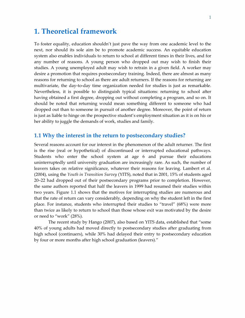
This paper will focus in particular on interrupted educational pathways, in a bid to
understand what causes adults — both those who complete their initial programs and
those who drop out — to return to postsecondary studies. More specifically, we will
attempt to answer two questions:
1. When is the return to postsecondary education most common?
2. What factors influence adults to resume postsecondary studies?
Our approach is based on statistical analyses that monitor a student cohort’s
educational pathways over successive semesters, thus enabling us to identify the points of
exit and return.
1 For our purposes, the notion of “adult,” a somewhat problematic term, is based on two general definitions. The first, after
Galland (1991), describes as an adult as someone possessing social autonomy: an employed individual who has left the
childhood home to found his or her own household. Having completed initial education, an adult — if he or she is in school
— is someone who has returned. The second definition has currency in the field of adult education, and denotes an adult
student as someone who left school for a significant period (e.g. 6-12 months) before returning. In some cases, an age
criterion is proposed: an adult is someone aged 25 and over. In all definitions, the adult learner is a person who has resumed
studies after a period away.

viii WHEN YOUNG CANADIAN ADULTS RETURN TO SCHOOL
1
1. Theoretical framework
To foster equality, education shouldn’t just pave the way from one academic level to the
next, nor should its sole aim be to promote academic success. An equitable education
system also enables individuals to return to school at different times in their lives, and for
any number of reasons. A young person who dropped out may wish to finish their
studies. A young unemployed adult may wish to retrain in a given field. A worker may
desire a promotion that requires postsecondary training. Indeed, there are almost as many
reasons for returning to school as there are adult returners. If the reasons for returning are
multivariate, the day-to-day time organization needed for studies is just as remarkable.
Nevertheless, it is possible to distinguish typical situations: returning to school after
having obtained a first degree, dropping out without completing a program, and so on. It
should be noted that returning would mean something different to someone who had
dropped out than to someone in pursuit of another degree. Moreover, the point of return
is just as liable to hinge on the prospective student’s employment situation as it is on his or
her ability to juggle the demands of work, studies and family.
1.1 Why the interest in the return to postsecondary studies?
Several reasons account for our interest in the phenomenon of the adult returner. The first
is the rise (real or hypothetical) of discontinued or interrupted educational pathways.
Students who enter the school system at age 6 and pursue their educations
uninterruptedly until university graduation are increasingly rare. As such, the number of
leavers takes on relative significance, whatever their reasons for leaving. Lambert et al.
(2004), using the Youth in Transition Survey (YITS), noted that in 2001, 15% of students aged
20–22 had dropped out of their postsecondary programs prior to completion. However,
the same authors reported that half the leavers in 1999 had resumed their studies within
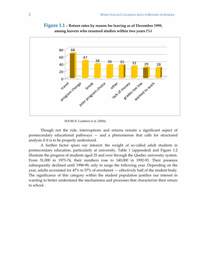
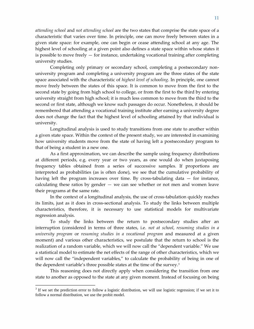
two years. Figure 1.1 shows that the motives for interrupting studies are numerous and
that the rate of return can vary considerably, depending on why the student left in the first
place. For instance, students who interrupted their studies to “travel” (68%) were more
than twice as likely to return to school than those whose exit was motivated by the desire
or need to “work” (28%).
The recent study by Hango (2007), also based on YITS data, established that “some
40% of young adults had moved directly to postsecondary studies after graduating from
high school (continuers), while 30% had delayed their entry to postsecondary education
by four or more months after high school graduation (leavers).”
2 WHEN YOUNG CANADIAN ADULTS RETURN TO SCHOOL
Figure 1.1 – Return rates by reason for leaving as of December 1999,
among leavers who resumed studies within two years (%)
SOURCE: Lambert et al. (2004).
Though not the rule, interruptions and returns remain a significant aspect of
postsecondary educational pathways — and a phenomenon that calls for structured
analysis if it is to be properly understood.
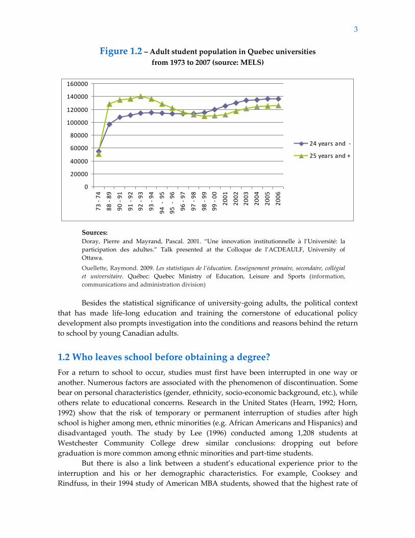
A further factor spurs our interest: the weight of so-called adult students in
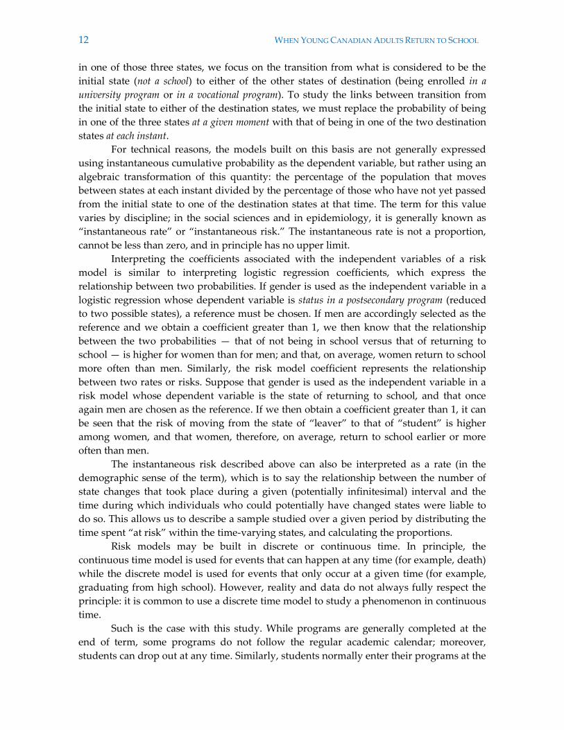
postsecondary education, particularly at university. Table 1 (appended) and Figure 1.2
illustrate the progress of students aged 25 and over through the Quebec university system.
From 51,000 in 1973-74, their numbers rose to 140,000 in 1992-93. Their presence
subsequently declined until 1998-99, only to surge the following year. Depending on the
year, adults accounted for 47% to 57% of enrolment — effectively half of the student body.
The significance of this category within the student population justifies our interest in
wanting to better understand the mechanisms and processes that characterize their return
to school.
68
4738 36 35 32 29 28
0
20
40
60
80
travel
progra
m change
break
poor pro
gram
choice
other
lack o
f money
grades t
oo low
wanted to
work
3
Figure 1.2 – Adult student population in Quebec universities
from 1973 to 2007 (source: MELS)
0
20000
40000
60000
80000
100000
120000
140000
160000
73
- 7
4
88
- 8
9
90
- 9
1
91
- 9
2
92
- 9
3
93
- 9
4
94
- 9
5
95
- 9
6
96
- 9
7
97
- 9
8
98
- 9
9
99
- 0
0
20
01
20
02
20
03
20
04
20
05
20
06
24 years and -
25 years and +
Sources: Doray, Pierre and Mayrand, Pascal. 2001. “Une innovation institutionnelle à l’Université: la
participation des adultes.” Talk presented at the Colloque de l’ACDEAULF, University of
Ottawa.
Ouellette, Raymond. 2009. Les statistiques de l’éducation. Enseignement primaire, secondaire, collégial
et universitaire. Québec: Quebec Ministry of Education, Leisure and Sports (information,
communications and administration division)
Besides the statistical significance of university-going adults, the political context
that has made life-long education and training the cornerstone of educational policy
development also prompts investigation into the conditions and reasons behind the return
to school by young Canadian adults.
1.2 Who leaves school before obtaining a degree?
For a return to school to occur, studies must first have been interrupted in one way or
another. Numerous factors are associated with the phenomenon of discontinuation. Some
bear on personal characteristics (gender, ethnicity, socio-economic background, etc.), while
others relate to educational concerns. Research in the United States (Hearn, 1992; Horn,
1992) show that the risk of temporary or permanent interruption of studies after high
school is higher among men, ethnic minorities (e.g. African Americans and Hispanics) and
disadvantaged youth. The study by Lee (1996) conducted among 1,208 students at
Westchester Community College drew similar conclusions: dropping out before
graduation is more common among ethnic minorities and part-time students.
But there is also a link between a student’s educational experience prior to the
interruption and his or her demographic characteristics. For example, Cooksey and
Rindfuss, in their 1994 study of American MBA students, showed that the highest rate of
4 WHEN YOUNG CANADIAN ADULTS RETURN TO SCHOOL
non-completion occurred among part-time students. Given that individuals from low to
middle socioeconomic backgrounds are more likely to enrol on a part-time basis, their risk
of interrupting their studies before completing their program is thus higher than that of
their wealthier counterparts. In England, Davies and Elias (2003) showed that students
who dropped out were likely faced with an unsatisfactory course choices or financial or
personal problems.
In Canada, the study by Tomkowicz and Bushnik (2003) showed that delayers (high
school graduates who enter postsecondary education following a hiatus) differ from right-
awayers (those who enrol directly after high school) in terms of both demographics and
educational background. Members of the former category show a higher proportion of
married individuals and individuals with children or dependents. Overall, the proportion
of delayers is higher among men, rural residents and families in which neither parent has
a university education. In terms of social and academic experience, delayers often have
lower grades and show a lower level of commitment to school; moreover, they often
belong to groups of students who, in high school, do not intend to pursue and show little
interest in postsecondary education. In terms of their distribution, delayers are
proportionally higher in Prince Edward Island, Saskatchewan, Alberta and British
Columbia than in Ontario, but lower in Quebec.
Other Canadian studies also show a higher predisposition among delayers to
interrupt their studies. Lambert et al. (2004), whose study uses data from the Youth in
Transition Survey Cohort B (ages 18–20), presents students who leave their postsecondary
programs prior to completion as having distinct social and academic characteristics. Their
proportion is higher among respondents who are male and/or in a couple, have dependent
children, or live with one parent (or in a household other than a two-parent family). Non-
completion is far less common among students who have at least one parent with a
postsecondary degree. People whose parents attach importance to postsecondary
education are less likely to drop out.
As regards schooling, Lambert et al. (2004) also observed that students who leave
before completing their programs show weak levels of commitment and preparation as
well as distinctive psychosocial traits. They are less motivated to study, displaying instead
a marked interest in paid work and/or travel. They have difficulty adapting to the
demands of academia, and struggle with the workload and pace imposed by the school.
They have low grades, are frequently dissatisfied and tend to want to change their
program or leave it altogether.
In sum, a cause-and-effect relationship appears to exist between the tendency to
interrupt studies and social background, living conditions, commitment to education,
academic goals, and the characteristics of the educational experience.
1.3 Returning to school: what does it consist of?
Numerous factors may prompt someone to return to school. Nonetheless, according to
Berger and Luckmann (1992) and Leclerc-Olive (1993), whatever its cause, the return to
education aligns with a twofold process of biographical disruption and conversion. In this
sense, adults who choose to return to school are motivated by the desire to make amends
5
for the past (“biographical accidents”) or to create new professional opportunities. Both
disruption and conversion essentially use the acquisition of new skills as a means of
connecting the dots between past and future. The return is part of a profound self-
interrogation process by someone who questions his or her place in society and
subsequently decides to change his or her life course to create a new social reality. In so
doing, individuals disaffiliate with their previous lives:
Going back to school is a way of intentionally signalling discontinuity. It formalizes
the break, enabling it to occur through the creation of a new social reality. In this
context, the university is a resocialization structure in the life of the individual. Going
back to school enables both the objectivation of disruption and biographical conversion.
[Translation] (Berger and Luckmann, 1992, p. 18)
The dual process of disruption/conversion entails the construction of a space where
identity formation and transformation can occur. In many cases, adults who return to
school are concerned with legitimating their professional status, obtaining a promotion or
gaining social currency. Such a conversion precedes life-course disruption, of which
authors distinguish two types. In the first, the return to school can represent an upheaval
to private life (disruption 1) in that it is liable to disrupt to a certain degree the individual’s
history or family life. In the second, it represents a rupture to participation in public life
(disruption 2), since returning to university represents integration into a relatively new space
that differs from the previous situation.
Who goes back to school?
We can group the many factors that can motivate a return to school into three main
categories: sociodemographic characteristics, previous education and living conditions.
Sociodemographic characteristics
Returning to school is less likely among socially disadvantaged groups, who are also more
likely to interrupt their studies. In the United States, having dependent children reduces
the probability of returning to school (Kwong, Mok and Kwong, 1997). While belonging to
an ethnic minority (e.g. African American, Hispanic) initially reduces the probability, the
influence of ethnicity diminishes when other factors like family background and socio-
economic status of a person’s occupation come into play (Marcus, 1986).
Previous education
Generally speaking, the return to school is motivated by factors related to the initial
reasons that caused the interruption. Davey and Jamieson (2003) cite three types of
interruption. In the first, the student leaves in spite of good grades and a positive attitude
toward education. In this case, leaving is often related to financial constraints or family
responsibilities; correspondingly, the return to school is generally motivated by the desire
to acquire new knowledge. The second type of interruption is associated with a lack of
self-confidence and includes individuals who, unsure of their academic capabilities, see no
point to further studies. Here, the return to school is often part of a broader personal
transition (e.g. change in the wake of divorce, job loss, etc.); motivation frequently comes
6 WHEN YOUNG CANADIAN ADULTS RETURN TO SCHOOL
from peers, whose encouragement helps compensate for any lacking confidence. In the
third type, dropping out is associated with an act of rebellion, often in conjunction with
behaviour problems and negative attitudes toward schooling. This is especially true for
those who leave in search of paid employment or “freedom.”
The decision to return to school is also influenced by previous education.
Individuals whose educational experience has been positive are more liable to resume
studies, since they tend to have higher educational goals overall and aim for higher levels
of training. If, however, a relatively high degree of previous schooling raises the hazard of
return, this tendency falls progressively over time (Marcus, 1986): the longer the
interruption, the less likely the chance of returning.
Living conditions
A close connection exists between returning to school and life after the initial interruption.
Individuals who resume studies are often motivated by a desire to improve their situation.
Apt Harper (1978) identifies five key factors, both positive and negative, that play into the
return to school among adults: personal development goals, the desire for knowledge,
career objectives, situational barriers, and emotional obstacles. These factors are liable to
be affected in turn by personal characteristics such as age, income, conjugal status, gender
and previous education. For example, age, conjugal status and occupation can influence
career goals; similarly, income, gender and conjugal status can serve as situational
barriers.
A longitudinal survey of 17,500 young Americans at ages 7, 11, 16, 23 and 33 found
that good working conditions tend to hinder the return to school after an interruption
(Thomas, 2001). A job that matched career aspirations reduced the hazard of returning to
school, especially when it corresponded to the individual’s capacities and qualifications.
Conversely, a job that was a poor match with career aspirations served to stoke feelings of
frustration and fuel the hazard of returning to school. Similarly, Marcus (1986) found that
the higher the wage, the lower the motivation to resume studying, and the same in
reverse. According to Marcus, the return to school is less common among workers with
good jobs (“lucky workers”) than among those working under less attractive conditions
(“unlucky workers”). Simply put, people who like their work are more apt to keep on
working. Smart and Pascarella (1987) have highlighted the relationship between
organization size, working conditions, type of employment and returning to school.
Furthermore, going back to school appears to be strongly influenced by current or
anticipated living conditions: for instance, according to Goldberg (1985), the prospect of
receiving a scholarship can incite adults to return to school even when they have jobs or
family responsibilities.
1.4 Perseverance after returning
Findings from Horn and Carroll (1998) drawing on data from the U.S.-based 1989-1990
Beginning Postsecondary Longitudinal Study showed that 16% of students who entered a
university program interrupted their studies in their first year. Among this number, 64%
resumed their schooling within five years of the interruption. Those who returned to the
7
same school did so more rapidly and had a higher probability of completing their program
than those who changed schools. Additionally, students at private schools were more
likely to complete their programs than those who attended public institutions.
Post-return perseverance tends to rise with the level of engagement. According to
Lee (1996), perseverance is highest among students with a personal interest in their
programs and a deep commitment to being a student. Conversely, it is lower among part-
time, ethnic minority and male students.
Research by Malloch and Montgomery (1996) with students from Maryland
University College draws similar conclusions. Adults who resume studies after a
relatively long interruption show lower levels of academic perseverance than do those
whose pathway is more traditional (continuous). The former are also more likely to drop
out for a second time before obtaining a degree. This breach in perseverance is not
attributable to age, but rather to the absence of sustained academic goals. Certain social
groups — African Americans and Aboriginal peoples being but two examples — are also
at a higher risk.
If, in general, an interrupted pathway reduces the hazard of obtaining
postsecondary qualifications, the level of education at the point of interruption appears to
be significant. According to Cooksey and Rindfuss (1994), adults who diverge from the
educational pathway straight after high school and then return to university are at a higher
risk of interrupting their studies for a second time or of never completing a postsecondary
program. Conversely, taking a break from schooling after graduation from an
undergraduate program does not appear to reduce the hazard of going back to obtain a
master’s or higher degree; students who tend to do so have generally engaged in some
sort of professional activity after their undergraduate degrees.
1.5 Summary
The studies consulted in this report would indicate that the flexible measures
implemented to facilitate adult access to higher education have had positive results: adult
participation in postsecondary studies has increased over the years. In most cases, adult
returners do so either to complete an unfinished program or to embark upon a new one.
The main advantage of the flexible measures is their ability to correct — or at least
improve — the educational pathways of socially disadvantaged youth (a category that
includes youth who, due to inadequate training for job market entry, become at risk of
being so). Based on recent data, we aim to determine if the return to school among young
Canadians varies in relation to the time variable, and to what extent it may be influenced
by previous education, sociodemographic characteristics and living conditions.

8 WHEN YOUNG CANADIAN ADULTS RETURN TO SCHOOL
9
2. Methodology
2.1 About the survey and sample
This study uses data from the Youth in Transition Survey (YITS), a study jointly conducted
by Statistics Canada and Human Resources and Skills Development Canada. The YITS
questionnaires gathered data on significant aspects of the lives of young people, largely
regarding their periods of education or employment. The data was then used to study a
number of important transitions that can occur at this time of life, such as finishing high
school, embarking on postsecondary studies, obtaining a first job, leaving home, and so
on. The questionnaires also collected data on the factors liable to affect these transitions,
some of which — including family background and previous educational experience —
are “objective,” others of which (aspirations, expectations, and so on) are seen as
“subjective” (Statistics Canada, 2007: 83).
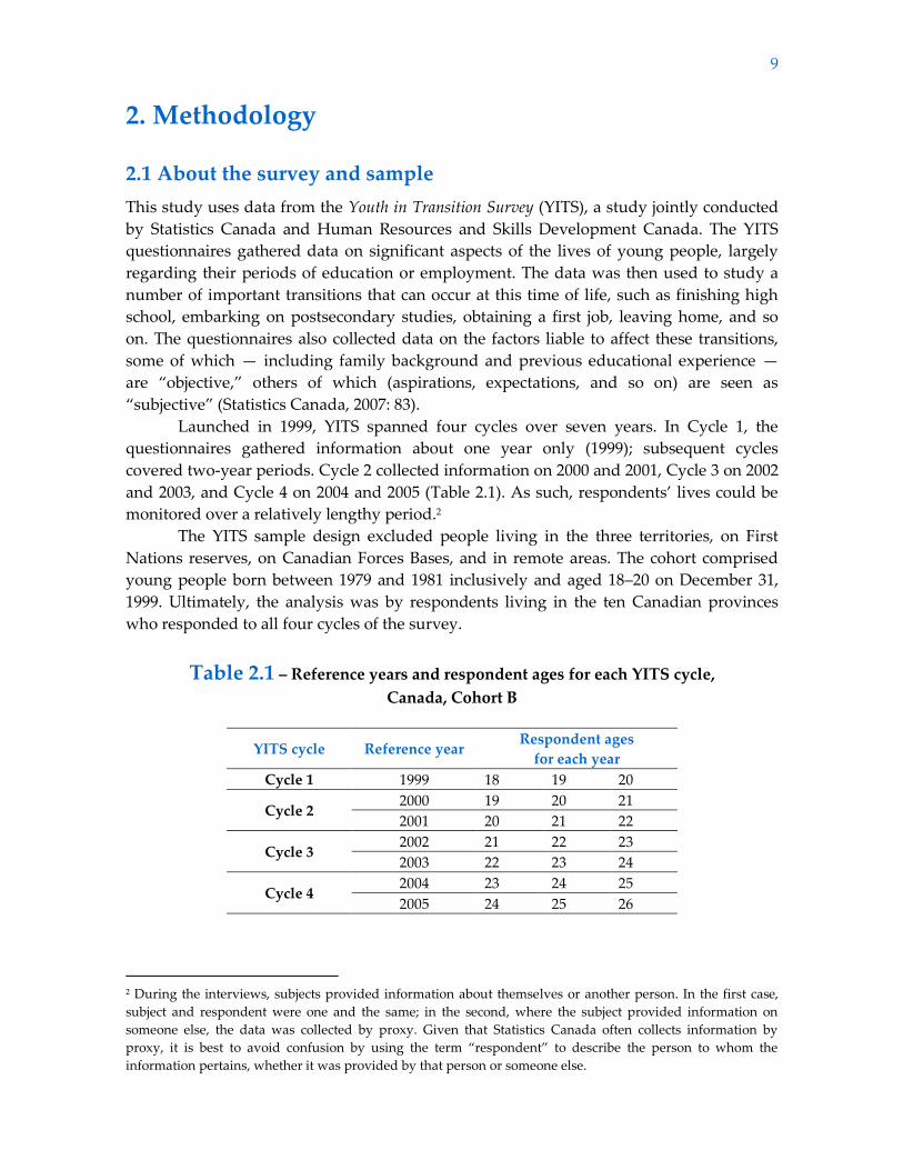
Launched in 1999, YITS spanned four cycles over seven years. In Cycle 1, the
questionnaires gathered information about one year only (1999); subsequent cycles
covered two-year periods. Cycle 2 collected information on 2000 and 2001, Cycle 3 on 2002
and 2003, and Cycle 4 on 2004 and 2005 (Table 2.1). As such, respondents’ lives could be
monitored over a relatively lengthy period.2
The YITS sample design excluded people living in the three territories, on First
Nations reserves, on Canadian Forces Bases, and in remote areas. The cohort comprised
young people born between 1979 and 1981 inclusively and aged 18–20 on December 31,
1999. Ultimately, the analysis was by respondents living in the ten Canadian provinces
who responded to all four cycles of the survey.
Table 2.1 – Reference years and respondent ages for each YITS cycle,
Canada, Cohort B
YITS cycle Reference year Respondent ages
for each year
Cycle 1 1999 18 19 20
Cycle 2 2000 19 20 21
2001 20 21 22
Cycle 3 2002 21 22 23
2003 22 23 24
Cycle 4 2004 23 24 25
2005 24 25 26
2 During the interviews, subjects provided information about themselves or another person. In the first case,
subject and respondent were one and the same; in the second, where the subject provided information on
someone else, the data was collected by proxy. Given that Statistics Canada often collects information by
proxy, it is best to avoid confusion by using the term “respondent” to describe the person to whom the
information pertains, whether it was provided by that person or someone else.
10 WHEN YOUNG CANADIAN ADULTS RETURN TO SCHOOL
Given the purpose of this paper, our analysis will focus on the return to school
after either a first degree or dropping out of a postsecondary program. The observation
period covers the years 1999 to 2005.
2.2 The cross-sectional approach, the longitudinal approach
and risk models
The cross-sectional approach is by far the most common in the social sciences; we mention
it here only as a means of introducing the longitudinal approach. In the former, a sample
is drawn from a population at a single point in time, and the resulting data are used to
describe the population at that time — providing what is sometimes described as a
“snapshot” of that population. The frequency distribution permits the sample to be
described using a range of characteristics such as gender, age, educational participation,
highest level of schooling, or highest grade/degree/certification. If the sample is
probabilistic, the distribution of a characteristic among that sample is seen to provide a
fairly accurate portrayal of that same characteristic’s distribution in the population, and
the only source of inaccuracy is sampling error. We are generally interested in the
frequency distribution, since it shows the proportional representation in the sample (and,
by extension, in the population) of each category of a given characteristic — for instance,
the percentages of men and women, or the proportion of the population that did not
advance beyond primary or secondary school, that only completed non-university
(college-equivalent) postsecondary studies, that attended university, and so on.
One might, for example, examine the highest level of schooling in each age group
of adults, knowing that the resulting table might have been different had the sample been
taken some years earlier or later (when the combination of prolonged studies and an aging
cohort would have increased the percentage of the adult population that had reached
university). However, examining the data from a single sample, taken at one time only,
does not allow this change to be seen. Changes only appear when similar samples drawn
at successive moments are juxtaposed.
While this approach has undeniable advantages, it fails to provide the information
necessary to understanding the evolution of the phenomenon studied. A longitudinal study
does not describe the population at a particular moment, nor does it show changes by
juxtaposing a succession of “snapshots.” Rather, it aims to make explicit the movement
through which change occurs. To conduct a longitudinal study in the sense that it is
understood here, the data must include biographical information about each individual in
the study population.
Conducting a longitudinal analysis means distinguishing fixed characteristics from
those that vary over time. Gender is one such fixed characteristic, as are first language, place
of birth and social origin, howsoever they may be assessed. Attending school, highest level of
schooling and employment status are characteristics that vary over time. More subtly, date of
birth is a fixed characteristic, while age varies directly in proportion to time.
The categories of these characteristics correspond to as many different states. The full
range of states of a given characteristic forms what is called the “state space.” Over time,
individuals can move from one state to another within a given characteristic. Thus,
11
attending school and not attending school are the two states that comprise the state space of a
characteristic that varies over time. In principle, one can move freely between states in a
given state space: for example, one can begin or cease attending school at any age. The
highest level of schooling at a given point also defines a state space within whose states it
is possible to move freely — for instance, undertaking vocational training after completing
university studies.
Completing only primary or secondary school, completing a postsecondary non-
university program and completing a university program are the three states of the state
space associated with the characteristic of highest level of schooling. In principle, one cannot
move freely between the states of this space. It is common to move from the first to the
second state by going from high school to college, or from the first to the third by entering
university straight from high school; it is much less common to move from the third to the
second or first state, although we know such passages do occur. Nonetheless, it should be
remembered that attending a vocational training institute after earning a university degree
does not change the fact that the highest level of schooling attained by that individual is
university.
Longitudinal analysis is used to study transitions from one state to another within
a given state space. Within the context of the present study, we are interested in examining
how university students move from the state of having left a postsecondary program to
that of being a student in a new one.
As a first approximation, we can describe the sample using frequency distributions
at different periods, e.g. every year or two years, as one would do when juxtaposing
frequency tables obtained from a series of successive samples. If proportions are
interpreted as probabilities (as is often done), we see that the cumulative probability of
having left the program increases over time. By cross-tabulating data — for instance,
calculating these ratios by gender — we can see whether or not men and women leave
their programs at the same rate.
In the context of a longitudinal analysis, the use of cross-tabulation quickly reaches
its limits, just as it does in cross-sectional analysis. To study the links between multiple
characteristics, therefore, it is necessary to use statistical models for multivariate
regression analysis.
To study the links between the return to postsecondary studies after an
interruption (considered in terms of three states, i.e. not at school, resuming studies in a
university program or resuming studies in a vocational program and measured at a given
moment) and various other characteristics, we postulate that the return to school is the
realization of a random variable, which we will now call the “dependent variable.” We use
a statistical model to estimate the net effects of the range of other characteristics, which we
will now call the “independent variables,” to calculate the probability of being in one of
the dependent variable’s three possible states at the time of the survey.3
This reasoning does not directly apply when considering the transition from one
state to another as opposed to the state at any given moment. Instead of focusing on being
3 If we set the prediction error to follow a logistic distribution, we will use logistic regression; if we set it to
follow a normal distribution, we use the probit model.
12 WHEN YOUNG CANADIAN ADULTS RETURN TO SCHOOL
in one of those three states, we focus on the transition from what is considered to be the
initial state (not a school) to either of the other states of destination (being enrolled in a
university program or in a vocational program). To study the links between transition from
the initial state to either of the destination states, we must replace the probability of being
in one of the three states at a given moment with that of being in one of the two destination
states at each instant.
For technical reasons, the models built on this basis are not generally expressed
using instantaneous cumulative probability as the dependent variable, but rather using an
algebraic transformation of this quantity: the percentage of the population that moves
between states at each instant divided by the percentage of those who have not yet passed
from the initial state to one of the destination states at that time. The term for this value
varies by discipline; in the social sciences and in epidemiology, it is generally known as
“instantaneous rate” or “instantaneous risk.” The instantaneous rate is not a proportion,
cannot be less than zero, and in principle has no upper limit.
Interpreting the coefficients associated with the independent variables of a risk
model is similar to interpreting logistic regression coefficients, which express the
relationship between two probabilities. If gender is used as the independent variable in a
logistic regression whose dependent variable is status in a postsecondary program (reduced
to two possible states), a reference must be chosen. If men are accordingly selected as the
reference and we obtain a coefficient greater than 1, we then know that the relationship
between the two probabilities — that of not being in school versus that of returning to
school — is higher for women than for men; and that, on average, women return to school
more often than men. Similarly, the risk model coefficient represents the relationship
between two rates or risks. Suppose that gender is used as the independent variable in a
risk model whose dependent variable is the state of returning to school, and that once
again men are chosen as the reference. If we then obtain a coefficient greater than 1, it can
be seen that the risk of moving from the state of “leaver” to that of “student” is higher
among women, and that women, therefore, on average, return to school earlier or more
often than men.
The instantaneous risk described above can also be interpreted as a rate (in the
demographic sense of the term), which is to say the relationship between the number of
state changes that took place during a given (potentially infinitesimal) interval and the
time during which individuals who could potentially have changed states were liable to
do so. This allows us to describe a sample studied over a given period by distributing the
time spent “at risk” within the time-varying states, and calculating the proportions.
Risk models may be built in discrete or continuous time. In principle, the
continuous time model is used for events that can happen at any time (for example, death)
while the discrete model is used for events that only occur at a given time (for example,
graduating from high school). However, reality and data do not always fully respect the
principle: it is common to use a discrete time model to study a phenomenon in continuous
time.
Such is the case with this study. While programs are generally completed at the
end of term, some programs do not follow the regular academic calendar; moreover,
students can drop out at any time. Similarly, students normally enter their programs at the
13
beginning of a semester, but programs that do not follow the regular academic calendar
allow students to return to school at any time. The event of interest — the return to school
— follows a pattern that is to a large degree established by the regular academic calendar,
but that nonetheless allows for many exceptions. If it followed the calendar, it could be
rigorously examined using a discrete time model. Our use of this model is based on the
following: the somewhat hybrid nature of the return-to-school patterns, the relative
inaccuracy of the YITS dates, and the fact that it seems unreasonable to assume, a priori,
that the factors of interest produce effects that do not vary within the time elapsed since
leaving studies.
2.3 The event studied and the at-risk group
In this section, we will examine operational definitions of the event under study and the
group at risk of experiencing it.
Postsecondary programs The YITS collected dated information on each respondent’s periods of postsecondary
studies between January 1999 and December 2005. For the purposes of the YITS, an
eligible postsecondary program “is one that is above the high school level; is towards a
diploma, certificate or degree; [and] would take someone three months or more to
complete.” The program must have begun before December 31 of the previous year’s
reference period (Statistics Canada, 2007: 13).
Postsecondary program levels The data collected through the YITS questionnaires cannot, in all cases, directly determine
whether or not the “eligible postsecondary program” is a university, pre-university or
vocational program. To identify respondents’ programs, we combined the collected data
related to the program “level” with those pertaining to the institution’s “type” and name,
the time required to complete the program (as a full-time student), and the province where
the institution was located. The question is more complex with regard to studies in
Quebec, since the YITS questionnaires did not accurately distinguish vocational training
from the pre-university programs offered through the CEGEPs.
For our purposes, programs that met at least one of the following criteria were
considered at the university level:
Programs offered in what was clearly a university-type institution in Quebec or
the rest of Canada
Undergraduate programs in Quebec or elsewhere in Canada; or undergraduate
programs offered in Quebec and preceded by a pre-university college program
(to the extent we were able to identify such programs)
College-level programs offered elsewhere in Canada, of at least four years’
duration (full-time)
Programs reported by the respondent as “postgraduate or graduate,”
“university certificate lower than an undergraduate degree,” “university
14 WHEN YOUNG CANADIAN ADULTS RETURN TO SCHOOL
certificate or degree above the undergraduate but beneath the master’s degree,”
“master’s program” or “PhD program.”
Programs were considered pre-university when:
They were college-level programs offered at a Quebec-based college and lasting
two to under three years full-time
They were described by the respondent as being a pre-university program
offered by a college or CEGEP (to obtain credits, a pre-university diploma or an
associate degree)
Programs were considered vocational when:
They were described by respondents as being a diploma or certificate program
at a private commercial school or training institute, a registered apprenticeship
program or an attestation of vocational specialization
They were college-level programs offered at a Quebec-based CEGEP lasting up
to three years on a full-time basis
They were a college-level program lasting less than four years on a full-time
basis in a community college in the rest of Canada (outside of Quebec)
Respondents’ postsecondary status
The YITS noted the dates respondents began their programs as well as their dates of final
enrolment. The database also contained a derived variable indicating whether, at the time
of the survey, each individual was still enrolled in the program, had completed it or had
dropped out.4 We selected programs for which such information was available. Apart
from Cycle 1, each YITS cycle covered two years; however, it is common for students to
spend more than two years in a given program. In the database, each program followed by
a respondent was associated with an identifier. The identifier indicated information on the
program throughout the cycles,5 thus allowing us to determine an individual’s
postsecondary status for each semester. The possible situations were as follows: not in
school, in a university program, in a pre-university program and in a vocational program.
Leaving postsecondary studies
For our purposes, respondents were considered to have left postsecondary education in
the semester in which they obtained their degree or were otherwise last enrolled prior to
leaving. Respondents were not considered to have left postsecondary education if they
were enrolled in other programs during that semester or had started another program
during the fall or winter semester following that semester. When a respondent left more
than one program in the same semester, we chose the program whose “level” was the
highest.
4 In YITS terminology, an individual still enrolled in a program is a “continuer”; one who has completed a
program, a “graduate”; and one who has dropped out, a “leaver.” 5 The identifier was a four-digit code that identified the following: the cycle in which the respondent had
begun the program, the program’s rank and the institution’s rank during the cycle in which the respondent
had begun the program. Programs retained the same identifier throughout the YITS cycles.
15
Returning to school
We chronologically ordered the postsecondary education programs in which respondents
had been registered between 1999 and 2005. This allowed us to identify the programs
undertaken by respondents after an interruption (whether the interruption had followed
completion of a first program or the abandonment of a program that would have yielded a
first degree). When an individual had started more than one program in the same
semester, we chose the program whose “level” was the highest. Returns during the winter
term corresponded to programs that started between January and May of that year;
returns during the fall semester, to programs that started between August and December
of that year.
The at-risk group
Our investigation focused on the return to postsecondary studies among adult students
who had obtained or failed to obtain a first degree. In methodological terms, young people
become “at risk” of returning to school two terms after first leaving (with or without
diploma). They were no longer “at risk” once they started a new program or ceased being
under observation while still out of school (i.e. at the end of the period covered by Cycle
4). An individual who returned to school left the at-risk group by changing his or her
status from leaver to student; an individual who stopped being observed while still out of
school left the at-risk group without changing states.
2.4 Operationalizing independent variables
The YITS data enabled us to examine how three aspects of young people’s lives influenced
their educational pathways:
Living conditions: employment status (working/not working) and the
characteristics of jobs held during employment periods
Sociodemographic features: area of residence, gender, conjugal status, having
children or not, parental educational capital
Previous education: level of the program that had yielded the first degree or that the
student had left without completing
The independent variables used in a life-course analysis like this study must apply
the same logic as the dependent variables. It is expected that most independent variables
examined here have categories that can change while the individual is “at risk” of
returning to school; as such, these are time-varying variables. The analysis requires data
related to the state change dates within each independent variable. For example, using
employment start and end dates, we can create a time-varying covariate whose state space
is defined by the shift from the state of inactivity to the state of working and vice versa
throughout an individual’s educational pathway.
We classed YITS variables into three groups, according to the precision with which
data on changes to value had been recorded.
1) Time-varying covariates, whose categories were assessed monthly and yearly (e.g.
employment status, number of jobs). Using these variables, we derived the month-
16 WHEN YOUNG CANADIAN ADULTS RETURN TO SCHOOL
by-month value of employment period characteristics whose monthly values
during this period were unknown: for instance, income and number of hours
worked (assessed at the job start and end dates); class of worker, work pattern and
occupational skill level (assessed at the start of employment only).
2) Time-varying covariates, whose categories were assessed every two years (e.g.
living arrangements).
3) Fixed independent variables whose categories do not change over time (e.g. gender
or visible minority status).
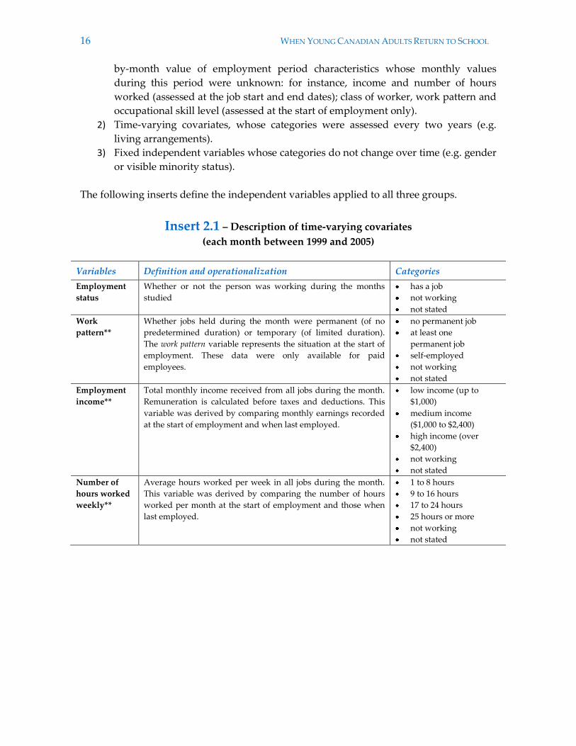
The following inserts define the independent variables applied to all three groups.
Insert 2.1 – Description of time-varying covariates
(each month between 1999 and 2005)
Variables Definition and operationalization Categories
Employment
status
Whether or not the person was working during the months
studied
has a job
not working
not stated
Work
pattern**
Whether jobs held during the month were permanent (of no
predetermined duration) or temporary (of limited duration).
The work pattern variable represents the situation at the start of
employment. These data were only available for paid
employees.
no permanent job
at least one
permanent job
self-employed
not working
not stated
Employment
income**
Total monthly income received from all jobs during the month.
Remuneration is calculated before taxes and deductions. This
variable was derived by comparing monthly earnings recorded
at the start of employment and when last employed.
low income (up to
$1,000)
medium income
($1,000 to $2,400)
high income (over
$2,400)
not working
not stated
Number of
hours worked
weekly**
Average hours worked per week in all jobs during the month.
This variable was derived by comparing the number of hours
worked per month at the start of employment and those when
last employed.
1 to 8 hours
9 to 16 hours
17 to 24 hours
25 hours or more
not working
not stated
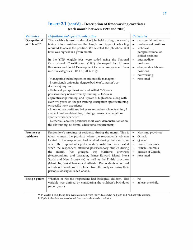
17
Insert 2.1 (cont’d) – Description of time-varying covariates
(each month between 1999 and 2005)
Variables Definition and operationalization Categories
Occupational
skill level**
This variable is used to describe jobs held during the month,
taking into consideration the length and type of schooling
required to access the position. We selected the job whose skill
level was highest in a given month.
In the YITS, eligible jobs were coded using the National
Occupational Classification (1991) developed by Human
Resources and Social Development Canada. We grouped them
into five categories (HRSDC, 2006: viii):
- Managerial: including senior and middle managers
- Professional: university degree (bachelor’s, master’s or
doctorate) required
- Technical, paraprofessional and skilled: 2–3 years
postsecondary non-university training, 2- to 5-year
apprenticeship training, or 3–4 years of high school along with
over two years’ on-the-job training, occupation-specific training
or specific work experience
- Intermediate positions: 1–4 years secondary school training, 2
years of on-the-job training, training courses or occupation-
specific work experience
- Elemental/labourer positions: short work demonstration or on-
the-job training; no formal educational requirements
managerial positions
professional positions
technical,
paraprofessional or
skilled positions
intermediate
positions
elemental or labourer
positions
not working
not stated
Province of
residence
Respondent’s province of residence during the month. This is
taken to mean the province where the respondent’s job was
located if the respondent had worked during the month, or
where the respondent’s postsecondary institution was located
when the respondent attended postsecondary studies during
the month. We grouped the Maritime provinces
(Newfoundland and Labrador, Prince Edward Island, Nova
Scotia and New Brunswick) as well as the Prairie provinces
(Manitoba, Saskatchewan and Alberta). Respondents who lived
outside of Canada were excluded from the analysis during their
period(s) of stay outside Canada.
Maritime provinces
Ontario
Quebec
Prairie provinces
British Columbia
outside of Canada
not stated
Being a parent Whether or not the respondent had biological children. This
variable was derived by considering the children’s birthdates
(month/year).
no
at least one child
** In Cycles 1 to 3, these data were collected from individuals who had jobs and had actively worked.
In Cycle 4, the data were collected from individuals who had jobs.
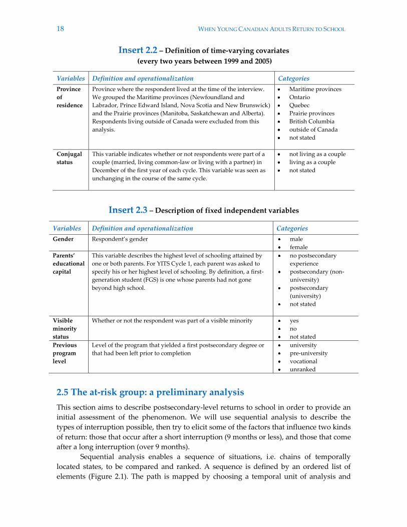
18 WHEN YOUNG CANADIAN ADULTS RETURN TO SCHOOL
Insert 2.2 – Definition of time-varying covariates
(every two years between 1999 and 2005)
Variables Definition and operationalization Categories
Province
of
residence
Province where the respondent lived at the time of the interview.
We grouped the Maritime provinces (Newfoundland and
Labrador, Prince Edward Island, Nova Scotia and New Brunswick)
and the Prairie provinces (Manitoba, Saskatchewan and Alberta).
Respondents living outside of Canada were excluded from this
analysis.
Maritime provinces
Ontario
Quebec
Prairie provinces
British Columbia
outside of Canada
not stated
Conjugal
status
This variable indicates whether or not respondents were part of a
couple (married, living common-law or living with a partner) in
December of the first year of each cycle. This variable was seen as
unchanging in the course of the same cycle.
not living as a couple
living as a couple
not stated
Insert 2.3 – Description of fixed independent variables
Variables Definition and operationalization Categories
Gender Respondent’s gender male
female
Parents’
educational
capital
This variable describes the highest level of schooling attained by
one or both parents. For YITS Cycle 1, each parent was asked to
specify his or her highest level of schooling. By definition, a first-
generation student (FGS) is one whose parents had not gone
beyond high school.
no postsecondary
experience
postsecondary (non-
university)
postsecondary
(university)
not stated
Visible
minority
status
Whether or not the respondent was part of a visible minority yes
no
not stated
Previous
program
level
Level of the program that yielded a first postsecondary degree or
that had been left prior to completion
university
pre-university
vocational
unranked
2.5 The at-risk group: a preliminary analysis
This section aims to describe postsecondary-level returns to school in order to provide an
initial assessment of the phenomenon. We will use sequential analysis to describe the
types of interruption possible, then try to elicit some of the factors that influence two kinds
of return: those that occur after a short interruption (9 months or less), and those that come
after a long interruption (over 9 months).
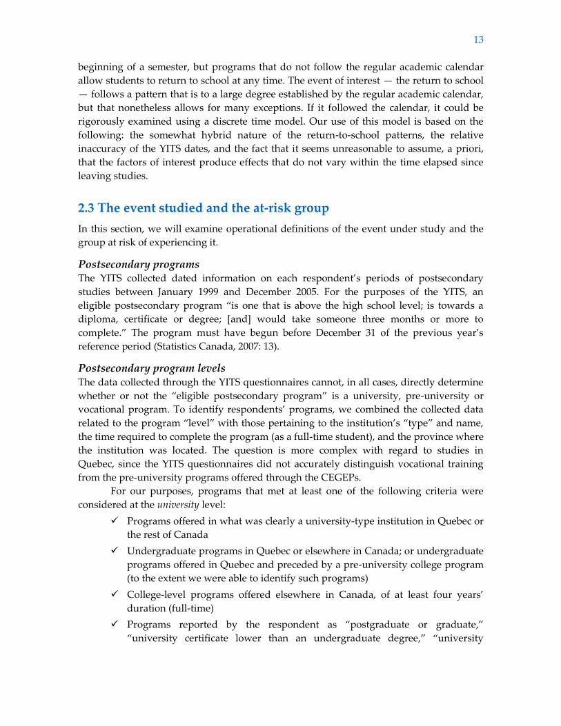
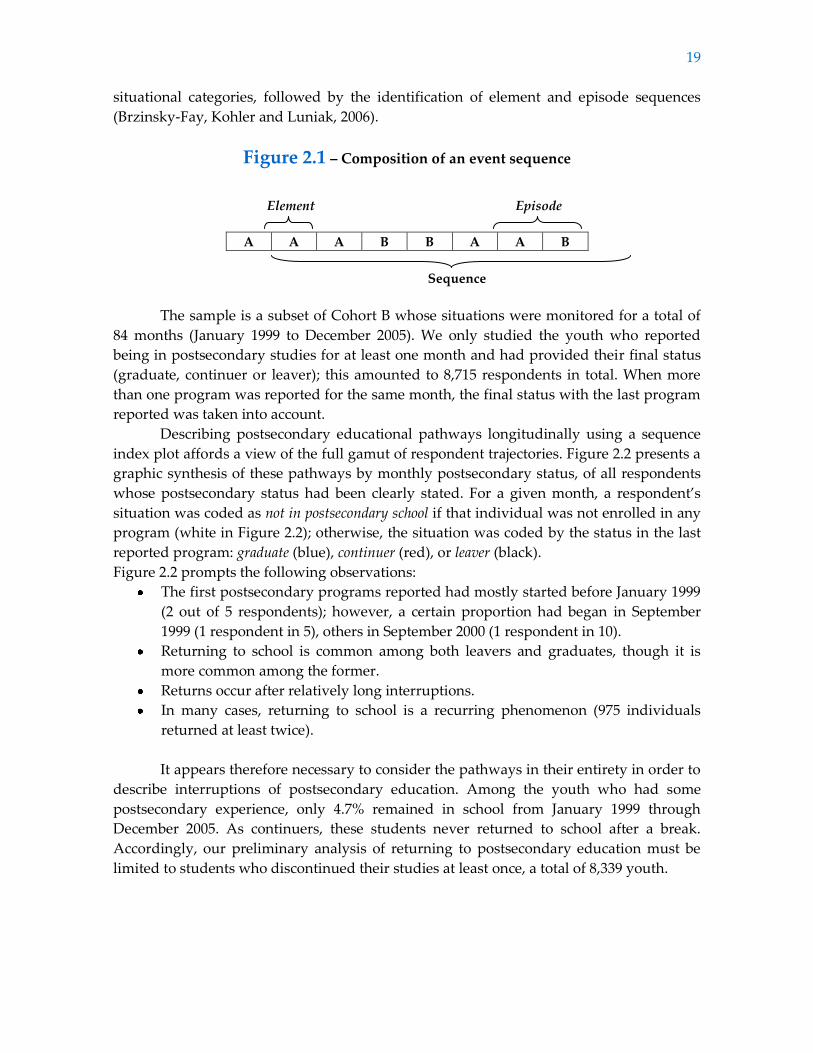
Sequential analysis enables a sequence of situations, i.e. chains of temporally
located states, to be compared and ranked. A sequence is defined by an ordered list of
elements (Figure 2.1). The path is mapped by choosing a temporal unit of analysis and
19
situational categories, followed by the identification of element and episode sequences
(Brzinsky-Fay, Kohler and Luniak, 2006).
Figure 2.1 – Composition of an event sequence
Element Episode
A A A B B A A B
Sequence
The sample is a subset of Cohort B whose situations were monitored for a total of
84 months (January 1999 to December 2005). We only studied the youth who reported
being in postsecondary studies for at least one month and had provided their final status
(graduate, continuer or leaver); this amounted to 8,715 respondents in total. When more
than one program was reported for the same month, the final status with the last program
reported was taken into account.
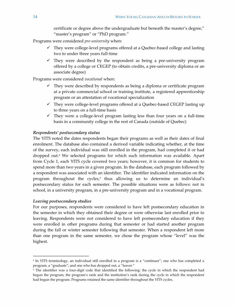
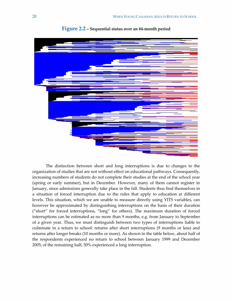
Describing postsecondary educational pathways longitudinally using a sequence
index plot affords a view of the full gamut of respondent trajectories. Figure 2.2 presents a
graphic synthesis of these pathways by monthly postsecondary status, of all respondents
whose postsecondary status had been clearly stated. For a given month, a respondent’s
situation was coded as not in postsecondary school if that individual was not enrolled in any
program (white in Figure 2.2); otherwise, the situation was coded by the status in the last
reported program: graduate (blue), continuer (red), or leaver (black).
Figure 2.2 prompts the following observations:
The first postsecondary programs reported had mostly started before January 1999
(2 out of 5 respondents); however, a certain proportion had began in September
1999 (1 respondent in 5), others in September 2000 (1 respondent in 10).
Returning to school is common among both leavers and graduates, though it is
more common among the former.
Returns occur after relatively long interruptions.
In many cases, returning to school is a recurring phenomenon (975 individuals
returned at least twice).
It appears therefore necessary to consider the pathways in their entirety in order to
describe interruptions of postsecondary education. Among the youth who had some
postsecondary experience, only 4.7% remained in school from January 1999 through
December 2005. As continuers, these students never returned to school after a break.
Accordingly, our preliminary analysis of returning to postsecondary education must be
limited to students who discontinued their studies at least once, a total of 8,339 youth.
20 WHEN YOUNG CANADIAN ADULTS RETURN TO SCHOOL
Figure 2.2 – Sequential status over an 84-month period
The distinction between short and long interruptions is due to changes to the
organization of studies that are not without effect on educational pathways. Consequently,
increasing numbers of students do not complete their studies at the end of the school year
(spring or early summer), but in December. However, many of them cannot register in
January, since admissions generally take place in the fall. Students thus find themselves in
a situation of forced interruption due to the rules that apply to education at different
levels. This situation, which we are unable to measure directly using YITS variables, can
however be approximated by distinguishing interruptions on the basis of their duration
(“short” for forced interruptions, “long” for others). The maximum duration of forced
interruptions can be estimated as no more than 9 months, e.g. from January to September
of a given year. Thus, we must distinguish between two types of interruptions liable to
culminate in a return to school: returns after short interruptions (9 months or less) and
returns after longer breaks (10 months or more). As shown in the table below, about half of
the respondents experienced no return to school between January 1999 and December
2005; of the remaining half, 50% experienced a long interruption.
21
Table 2.2 – Distribution of students by
type of interruption of postsecondary education
Situation %
Return to studies after a long interruption 24.3
Return to studies after a short interruption 24.2
Did not return to studies 51.5
Total 100
(N = 8,339)
The two situations are quite different. A preliminary descriptive analysis of the
determinants of both shows that many of the factors affecting the return to school after a
short interruption had no effect on returns following a long interruption. Two variables
serve to illustrate this difference: the province where the respondent’s first postsecondary
institution was located and final high school grades.
Whether the return to school came after a short or long interruption varied by
province of residence. Short interruptions were most common in Quebec (35.7%) and
Nova Scotia (30.8%). In Quebec, the existence of the CEGEPs as a transitional facility
between high school and university may account for this difference: CEGEP students are
likely to have their pathways forcibly interrupted since they are often unable to enrol in a
university program directly after finishing CEGEP.
Table 2.3 – Interruptions of postsecondary education
according to first-program characteristics (%)
First-program situation
Long
interruption
Short
interruption
Permanent
interruption
Final status
Degree obtained
Program not completed
19.6
32.9
23.7
25.2
56.6
41.9
Province
Newfoundland and Labrador
Prince Edward Island
Nova Scotia
New Brunswick
Quebec
Ontario
Manitoba
Saskatchewan
Alberta
British Columbia
22.5
28.3
22.2
23.3
23.0
23.5
26.3
22.9
26.7
26.4
18.3
19.0
30.8
22.5
35.7
20.4
15.4
16.9
23.1
19.4
59.2
52.8
47.0
54.2
41.3
56.1
58.3
60.2
50.1
54.2
Similarly, final grades in high school had a strong linear impact on returns
following short interruptions, but not on those following long interruptions. As shown in
Figure 2.3, only 40% of those whose overall high school average was between 90 and 100%
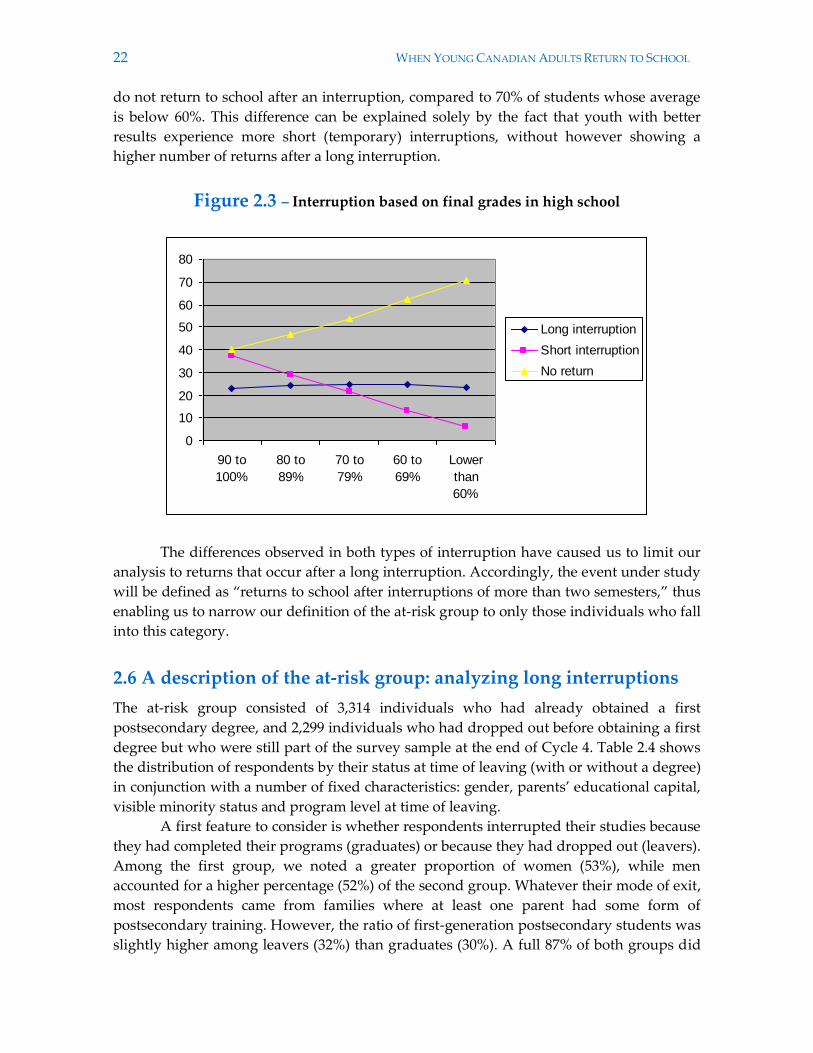
22 WHEN YOUNG CANADIAN ADULTS RETURN TO SCHOOL
do not return to school after an interruption, compared to 70% of students whose average
is below 60%. This difference can be explained solely by the fact that youth with better
results experience more short (temporary) interruptions, without however showing a
higher number of returns after a long interruption.
Figure 2.3 – Interruption based on final grades in high school
0
10
20
30
40
50
60
70
80
90 to
100%
80 to
89%
70 to
79%
60 to
69%
Lower
than
60%
Long interruption
Short interruption
No return
The differences observed in both types of interruption have caused us to limit our
analysis to returns that occur after a long interruption. Accordingly, the event under study
will be defined as “returns to school after interruptions of more than two semesters,” thus
enabling us to narrow our definition of the at-risk group to only those individuals who fall
into this category.
2.6 A description of the at-risk group: analyzing long interruptions
The at-risk group consisted of 3,314 individuals who had already obtained a first
postsecondary degree, and 2,299 individuals who had dropped out before obtaining a first
degree but who were still part of the survey sample at the end of Cycle 4. Table 2.4 shows
the distribution of respondents by their status at time of leaving (with or without a degree)
in conjunction with a number of fixed characteristics: gender, parents’ educational capital,
visible minority status and program level at time of leaving.
A first feature to consider is whether respondents interrupted their studies because
they had completed their programs (graduates) or because they had dropped out (leavers).
Among the first group, we noted a greater proportion of women (53%), while men
accounted for a higher percentage (52%) of the second group. Whatever their mode of exit,
most respondents came from families where at least one parent had some form of
postsecondary training. However, the ratio of first-generation postsecondary students was
slightly higher among leavers (32%) than graduates (30%). A full 87% of both groups did
23
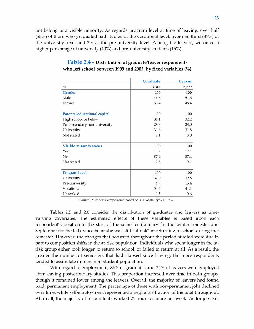
not belong to a visible minority. As regards program level at time of leaving, over half
(55%) of those who graduated had studied at the vocational level, over one third (37%) at
the university level and 7% at the pre-university level. Among the leavers, we noted a
higher percentage of university (40%) and pre-university students (15%).
Table 2.4 – Distribution of graduate/leaver respondents
who left school between 1999 and 2005, by fixed variables (%)
Graduate Leaver
N 3,314 2,299
Gender 100 100
Male 46.6 51.6
Female 53.4 48.4
Parents’ educational capital 100 100
High school or below 30.1 32.2
Postsecondary non-university 29.3 28.0
University 31.6 31.8
Not stated 9.1 8.0
Visible minority status 100 100
Yes 12.2 12.4
No 87.4 87.4
Not stated 0.5 0.1
Program level 100 100
University 37.0 39.8
Pre-university 6.9 15.4
Vocational 54.5 44.1
Unranked 1.5 0.6
Source: Authors’ extrapolation based on YITS data, cycles 1 to 4
Tables 2.5 and 2.6 consider the distribution of graduates and leavers as time-
varying covariates. The estimated effects of these variables is based upon each
respondent’s position at the start of the semester (January for the winter semester and
September for the fall), since he or she was still “at risk” of returning to school during that
semester. However, the changes that occurred throughout the period studied were due in
part to composition shifts in the at-risk population. Individuals who spent longer in the at-
risk group either took longer to return to school, or failed to return at all. As a result, the
greater the number of semesters that had elapsed since leaving, the more respondents
tended to assimilate into the non-student population.
With regard to employment, 83% of graduates and 74% of leavers were employed
after leaving postsecondary studies. This proportion increased over time in both groups,
though it remained lower among the leavers. Overall, the majority of leavers had found
paid, permanent employment. The percentage of those with non-permanent jobs declined
over time, while self-employment represented a negligible fraction of the total throughout.
All in all, the majority of respondents worked 25 hours or more per week. As for job skill
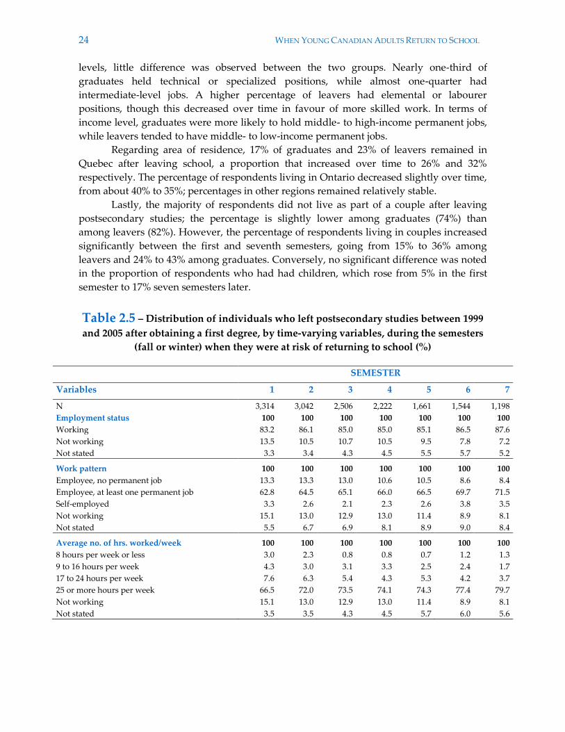
24 WHEN YOUNG CANADIAN ADULTS RETURN TO SCHOOL
levels, little difference was observed between the two groups. Nearly one-third of
graduates held technical or specialized positions, while almost one-quarter had
intermediate-level jobs. A higher percentage of leavers had elemental or labourer
positions, though this decreased over time in favour of more skilled work. In terms of
income level, graduates were more likely to hold middle- to high-income permanent jobs,
while leavers tended to have middle- to low-income permanent jobs.
Regarding area of residence, 17% of graduates and 23% of leavers remained in
Quebec after leaving school, a proportion that increased over time to 26% and 32%
respectively. The percentage of respondents living in Ontario decreased slightly over time,
from about 40% to 35%; percentages in other regions remained relatively stable.
Lastly, the majority of respondents did not live as part of a couple after leaving
postsecondary studies; the percentage is slightly lower among graduates (74%) than
among leavers (82%). However, the percentage of respondents living in couples increased
significantly between the first and seventh semesters, going from 15% to 36% among
leavers and 24% to 43% among graduates. Conversely, no significant difference was noted
in the proportion of respondents who had had children, which rose from 5% in the first
semester to 17% seven semesters later.
Table 2.5 – Distribution of individuals who left postsecondary studies between 1999
and 2005 after obtaining a first degree, by time-varying variables, during the semesters
(fall or winter) when they were at risk of returning to school (%)
SEMESTER
Variables 1 2 3 4 5 6 7
N 3,314 3,042 2,506 2,222 1,661 1,544 1,198
Employment status 100 100 100 100 100 100 100
Working 83.2 86.1 85.0 85.0 85.1 86.5 87.6
Not working 13.5 10.5 10.7 10.5 9.5 7.8 7.2
Not stated 3.3 3.4 4.3 4.5 5.5 5.7 5.2
Work pattern 100 100 100 100 100 100 100
Employee, no permanent job 13.3 13.3 13.0 10.6 10.5 8.6 8.4
Employee, at least one permanent job 62.8 64.5 65.1 66.0 66.5 69.7 71.5
Self-employed 3.3 2.6 2.1 2.3 2.6 3.8 3.5
Not working 15.1 13.0 12.9 13.0 11.4 8.9 8.1
Not stated 5.5 6.7 6.9 8.1 8.9 9.0 8.4
Average no. of hrs. worked/week 100 100 100 100 100 100 100
8 hours per week or less 3.0 2.3 0.8 0.8 0.7 1.2 1.3
9 to 16 hours per week 4.3 3.0 3.1 3.3 2.5 2.4 1.7
17 to 24 hours per week 7.6 6.3 5.4 4.3 5.3 4.2 3.7
25 or more hours per week 66.5 72.0 73.5 74.1 74.3 77.4 79.7
Not working 15.1 13.0 12.9 13.0 11.4 8.9 8.1
Not stated 3.5 3.5 4.3 4.5 5.7 6.0 5.6
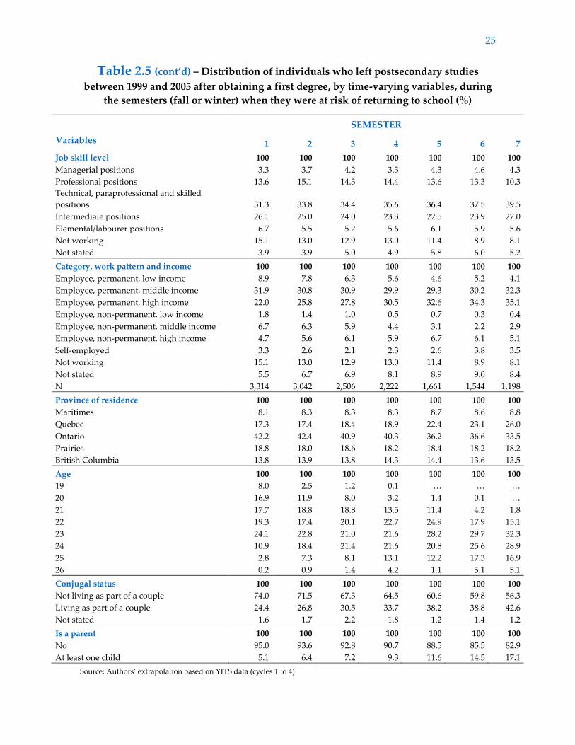
25
Table 2.5 (cont’d) – Distribution of individuals who left postsecondary studies
between 1999 and 2005 after obtaining a first degree, by time-varying variables, during
the semesters (fall or winter) when they were at risk of returning to school (%)
SEMESTER
Variables 1 2 3 4 5 6 7
Job skill level 100 100 100 100 100 100 100
Managerial positions 3.3 3.7 4.2 3.3 4.3 4.6 4.3
Professional positions 13.6 15.1 14.3 14.4 13.6 13.3 10.3
Technical, paraprofessional and skilled
positions 31.3 33.8 34.4 35.6 36.4 37.5 39.5
Intermediate positions 26.1 25.0 24.0 23.3 22.5 23.9 27.0
Elemental/labourer positions 6.7 5.5 5.2 5.6 6.1 5.9 5.6
Not working 15.1 13.0 12.9 13.0 11.4 8.9 8.1
Not stated 3.9 3.9 5.0 4.9 5.8 6.0 5.2
Category, work pattern and income 100 100 100 100 100 100 100
Employee, permanent, low income 8.9 7.8 6.3 5.6 4.6 5.2 4.1
Employee, permanent, middle income 31.9 30.8 30.9 29.9 29.3 30.2 32.3
Employee, permanent, high income 22.0 25.8 27.8 30.5 32.6 34.3 35.1
Employee, non-permanent, low income 1.8 1.4 1.0 0.5 0.7 0.3 0.4
Employee, non-permanent, middle income 6.7 6.3 5.9 4.4 3.1 2.2 2.9
Employee, non-permanent, high income 4.7 5.6 6.1 5.9 6.7 6.1 5.1
Self-employed 3.3 2.6 2.1 2.3 2.6 3.8 3.5
Not working 15.1 13.0 12.9 13.0 11.4 8.9 8.1
Not stated 5.5 6.7 6.9 8.1 8.9 9.0 8.4
N 3,314 3,042 2,506 2,222 1,661 1,544 1,198
Province of residence 100 100 100 100 100 100 100
Maritimes 8.1 8.3 8.3 8.3 8.7 8.6 8.8
Quebec 17.3 17.4 18.4 18.9 22.4 23.1 26.0
Ontario 42.2 42.4 40.9 40.3 36.2 36.6 33.5
Prairies 18.8 18.0 18.6 18.2 18.4 18.2 18.2
British Columbia 13.8 13.9 13.8 14.3 14.4 13.6 13.5
Age 100 100 100 100 100 100 100
19 8.0 2.5 1.2 0.1 < < <
20 16.9 11.9 8.0 3.2 1.4 0.1 <
21 17.7 18.8 18.8 13.5 11.4 4.2 1.8
22 19.3 17.4 20.1 22.7 24.9 17.9 15.1
23 24.1 22.8 21.0 21.6 28.2 29.7 32.3
24 10.9 18.4 21.4 21.6 20.8 25.6 28.9
25 2.8 7.3 8.1 13.1 12.2 17.3 16.9
26 0.2 0.9 1.4 4.2 1.1 5.1 5.1
Conjugal status 100 100 100 100 100 100 100
Not living as part of a couple 74.0 71.5 67.3 64.5 60.6 59.8 56.3
Living as part of a couple 24.4 26.8 30.5 33.7 38.2 38.8 42.6
Not stated 1.6 1.7 2.2 1.8 1.2 1.4 1.2
Is a parent 100 100 100 100 100 100 100
No 95.0 93.6 92.8 90.7 88.5 85.5 82.9
At least one child 5.1 6.4 7.2 9.3 11.6 14.5 17.1
Source: Authors’ extrapolation based on YITS data (cycles 1 to 4)
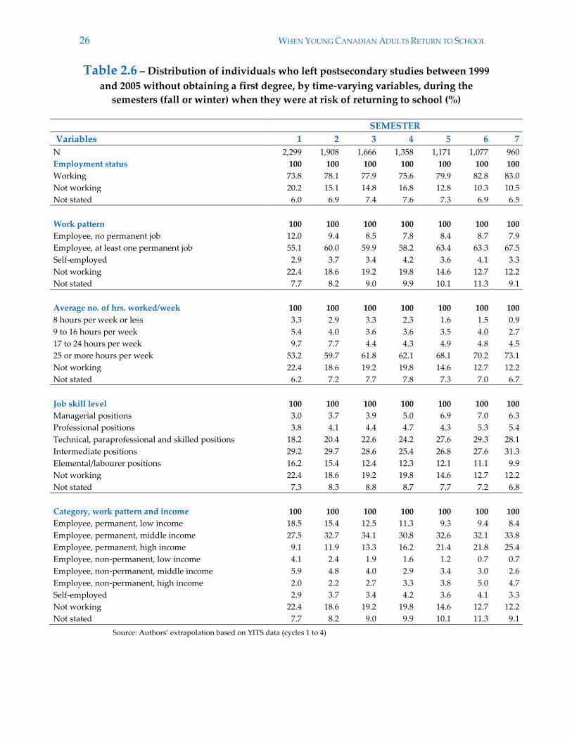
26 WHEN YOUNG CANADIAN ADULTS RETURN TO SCHOOL
Table 2.6 – Distribution of individuals who left postsecondary studies between 1999
and 2005 without obtaining a first degree, by time-varying variables, during the
semesters (fall or winter) when they were at risk of returning to school (%)
SEMESTER
Variables 1 2 3 4 5 6 7
N 2,299 1,908 1,666 1,358 1,171 1,077 960
Employment status 100 100 100 100 100 100 100
Working 73.8 78.1 77.9 75.6 79.9 82.8 83.0
Not working 20.2 15.1 14.8 16.8 12.8 10.3 10.5
Not stated 6.0 6.9 7.4 7.6 7.3 6.9 6.5
Work pattern 100 100 100 100 100 100 100
Employee, no permanent job 12.0 9.4 8.5 7.8 8.4 8.7 7.9
Employee, at least one permanent job 55.1 60.0 59.9 58.2 63.4 63.3 67.5
Self-employed 2.9 3.7 3.4 4.2 3.6 4.1 3.3
Not working 22.4 18.6 19.2 19.8 14.6 12.7 12.2
Not stated 7.7 8.2 9.0 9.9 10.1 11.3 9.1
Average no. of hrs. worked/week 100 100 100 100 100 100 100
8 hours per week or less 3.3 2.9 3.3 2.3 1.6 1.5 0.9
9 to 16 hours per week 5.4 4.0 3.6 3.6 3.5 4.0 2.7
17 to 24 hours per week 9.7 7.7 4.4 4.3 4.9 4.8 4.5
25 or more hours per week 53.2 59.7 61.8 62.1 68.1 70.2 73.1
Not working 22.4 18.6 19.2 19.8 14.6 12.7 12.2
Not stated 6.2 7.2 7.7 7.8 7.3 7.0 6.7
Job skill level 100 100 100 100 100 100 100
Managerial positions 3.0 3.7 3.9 5.0 6.9 7.0 6.3
Professional positions 3.8 4.1 4.4 4.7 4.3 5.3 5.4
Technical, paraprofessional and skilled positions 18.2 20.4 22.6 24.2 27.6 29.3 28.1
Intermediate positions 29.2 29.7 28.6 25.4 26.8 27.6 31.3
Elemental/labourer positions 16.2 15.4 12.4 12.3 12.1 11.1 9.9
Not working 22.4 18.6 19.2 19.8 14.6 12.7 12.2
Not stated 7.3 8.3 8.8 8.7 7.7 7.2 6.8
Category, work pattern and income 100 100 100 100 100 100 100
Employee, permanent, low income 18.5 15.4 12.5 11.3 9.3 9.4 8.4
Employee, permanent, middle income 27.5 32.7 34.1 30.8 32.6 32.1 33.8
Employee, permanent, high income 9.1 11.9 13.3 16.2 21.4 21.8 25.4
Employee, non-permanent, low income 4.1 2.4 1.9 1.6 1.2 0.7 0.7
Employee, non-permanent, middle income 5.9 4.8 4.0 2.9 3.4 3.0 2.6
Employee, non-permanent, high income 2.0 2.2 2.7 3.3 3.8 5.0 4.7
Self-employed 2.9 3.7 3.4 4.2 3.6 4.1 3.3
Not working 22.4 18.6 19.2 19.8 14.6 12.7 12.2
Not stated 7.7 8.2 9.0 9.9 10.1 11.3 9.1
Source: Authors’ extrapolation based on YITS data (cycles 1 to 4)
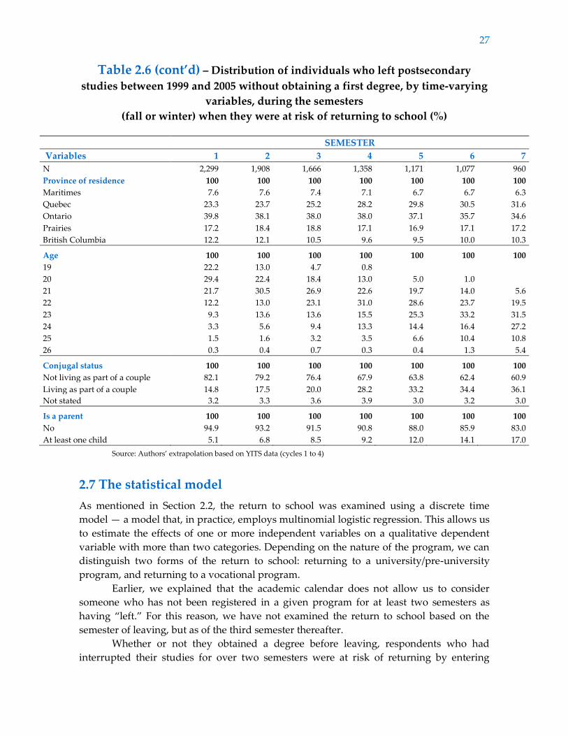
27
Table 2.6 (cont’d) – Distribution of individuals who left postsecondary
studies between 1999 and 2005 without obtaining a first degree, by time-varying
variables, during the semesters
(fall or winter) when they were at risk of returning to school (%)
SEMESTER
Variables 1 2 3 4 5 6 7
N 2,299 1,908 1,666 1,358 1,171 1,077 960
Province of residence 100 100 100 100 100 100 100
Maritimes 7.6 7.6 7.4 7.1 6.7 6.7 6.3
Quebec 23.3 23.7 25.2 28.2 29.8 30.5 31.6
Ontario 39.8 38.1 38.0 38.0 37.1 35.7 34.6
Prairies 17.2 18.4 18.8 17.1 16.9 17.1 17.2
British Columbia 12.2 12.1 10.5 9.6 9.5 10.0 10.3
Age 100 100 100 100 100 100 100
19 22.2 13.0 4.7 0.8
20 29.4 22.4 18.4 13.0 5.0 1.0
21 21.7 30.5 26.9 22.6 19.7 14.0 5.6
22 12.2 13.0 23.1 31.0 28.6 23.7 19.5
23 9.3 13.6 13.6 15.5 25.3 33.2 31.5
24 3.3 5.6 9.4 13.3 14.4 16.4 27.2
25 1.5 1.6 3.2 3.5 6.6 10.4 10.8
26 0.3 0.4 0.7 0.3 0.4 1.3 5.4
Conjugal status 100 100 100 100 100 100 100
Not living as part of a couple 82.1 79.2 76.4 67.9 63.8 62.4 60.9
Living as part of a couple 14.8 17.5 20.0 28.2 33.2 34.4 36.1
Not stated 3.2 3.3 3.6 3.9 3.0 3.2 3.0
Is a parent 100 100 100 100 100 100 100
No 94.9 93.2 91.5 90.8 88.0 85.9 83.0
At least one child 5.1 6.8 8.5 9.2 12.0 14.1 17.0
Source: Authors’ extrapolation based on YITS data (cycles 1 to 4)
2.7 The statistical model
As mentioned in Section 2.2, the return to school was examined using a discrete time
model — a model that, in practice, employs multinomial logistic regression. This allows us
to estimate the effects of one or more independent variables on a qualitative dependent
variable with more than two categories. Depending on the nature of the program, we can
distinguish two forms of the return to school: returning to a university/pre-university
program, and returning to a vocational program.
Earlier, we explained that the academic calendar does not allow us to consider
someone who has not been registered in a given program for at least two semesters as
having “left.” For this reason, we have not examined the return to school based on the
semester of leaving, but as of the third semester thereafter.
Whether or not they obtained a degree before leaving, respondents who had
interrupted their studies for over two semesters were at risk of returning by entering
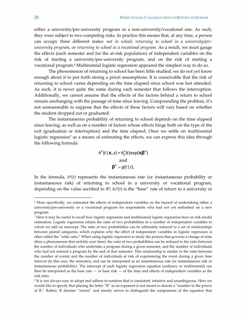
28 WHEN YOUNG CANADIAN ADULTS RETURN TO SCHOOL
either a university/pre-university program or a non-university/vocational one. As such,
they were subject to two competing risks. In practice this means that, at any time, a person
can occupy three different states: not in school, returning to school in a university/pre-
university program, or returning to school in a vocational program. As a result, we must gauge
the effects (each semester and for the at-risk population) of independent variables on the
risk of starting a university/pre-university program, and on the risk of starting a
vocational program.6 Multinomial logistic regression appeared the simplest way to do so.
The phenomenon of returning to school has been little studied; we do not yet know
enough about it to put forth strong a priori assumptions. It is conceivable that the risk of
returning to school varies depending on the time elapsed since school was last attended.
As such, it is never quite the same during each semester that follows the interruption.
Additionally, we cannot assume that the effects of the factors behind a return to school
remain unchanging with the passage of time since leaving. Compounding the problem, it’s
not unreasonable to suppose that the effects of these factors will vary based on whether
the student dropped out or graduated.
The instantaneous probability of returning to school depends on the time elapsed
since leaving, as well as on a number of factors whose effects hinge both on the type of the
exit (graduation or interruption) and the time elapsed. Once we settle on multinomial
logistic regression7 as a means of estimating the effects, we can express this idea through
the following formula:
0x xβ( | , ) ( )exp( )R R Rh t z h t
and
( | ),R g t zβ
In the formula, hR(t) represents the instantaneous rate (or instantaneous probability or
instantaneous risk) of returning to school in a university or vocational program,
depending on the value ascribed to R8; h0R(t) is the “base” rate of return to a university or
6 More specifically, we estimated the effects of independent variables on the hazard of undertaking either a
university/pre-university or a vocational program for respondents who had not yet embarked on a new
program. 7 Here it may be useful to recall how logistic regression and multinomial logistic regression bear on risk model
estimation. Logistic regression relates the ratio of two probabilities to a number of independent variables to
which we add an intercept. The ratio of two probabilities can be ultimately reduced to a set of relationships
between paired categories, which explains why the effect of independent variables in logistic regression is
often called the “odds ratio.” When using logistic regression to study the process that governs a change of state
(thus a phenomenon that unfolds over time), the ratio of two probabilities can be reduced to the ratio between
the number of individuals who undertake a program during a given semester, and the number of individuals
who had not entered a program by the end of that semester. This relationship is similar to the ratio between
the number of events and the number of individuals at risk of experiencing the event during a given time
interval (in this case, the semester), and can be interpreted as an instantaneous rate (or instantaneous risk or
instantaneous probability). The intercept of each logistic regression equation (ordinary or multinomial) can
then be interpreted as the base rate — or base risk — of the time and effects of independent variables as the
risk ratio. 8 It is not always easy to adopt and adhere to notation that is consistent, intuitive and unambiguous. Here we
would like to specify that placing the letter “R” as an exponent is not meant to denote a “number to the power
of R.” Rather, R denotes “return” and merely serves to distinguish the components of the equation that
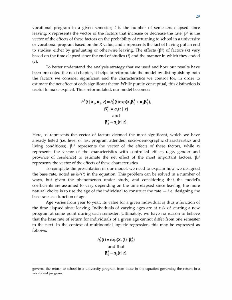
29
vocational program in a given semester; t is the number of semesters elapsed since
leaving; x represents the vector of the factors that increase or decrease the rate; βR is the
vector of the effects of these factors on the probability of returning to school in a university
or vocational program based on the R value; and z represents the fact of having put an end
to studies, either by graduating or otherwise leaving. The effects (βR) of factors (x) vary
based on the time elapsed since the end of studies (t) and the manner in which they ended
(z).
To better understand the analysis strategy that we used and how our results have
been presented the next chapter, it helps to reformulate the model by distinguishing both
the factors we consider significant and the characteristics we control for, in order to
estimate the net effect of each significant factor. While purely conceptual, this distinction is
useful to make explicit. Thus reformulated, our model becomes:
( | , , ) ( )exp( ),R R R Rh t z h tx x x β x β1 2 0 1 1 2 2
( )|R g t zβ1 1
and
( | ),R g t zβ2 2
Here, x1 represents the vector of factors deemed the most significant, which we have
already listed (i.e. level of last program attended, socio-demographic characteristics and
living conditions). β1R represents the vector of the effects of these factors, while x2
represents the vector of the characteristics with controlled effects (age, gender and
province of residence) to estimate the net effect of the most important factors. β2R
represents the vector of the effects of these characteristics.
To complete the presentation of our model, we need to explain how we designed
the base rate, noted as h0R(t) in the equation. This problem can be solved in a number of
ways, but given the phenomenon under study, and considering that the model’s
coefficients are assumed to vary depending on the time elapsed since leaving, the more
natural choice is to use the age of the individual to construct the rate — i.e. designing the
base rate as a function of age.
Age varies from year to year; its value for a given individual is thus a function of
the time elapsed since leaving. Individuals of varying ages are at risk of starting a new
program at some point during each semester. Ultimately, we have no reason to believe
that the base rate of return for individuals of a given age cannot differ from one semester
to the next. In the context of multinomial logistic regression, this may be expressed as
follows:
( ) exp( ( ) )R Rh t tx β0 0 0
and that
( | ),R g t zβ0 0
governs the return to school in a university program from those in the equation governing the return in a
vocational program.
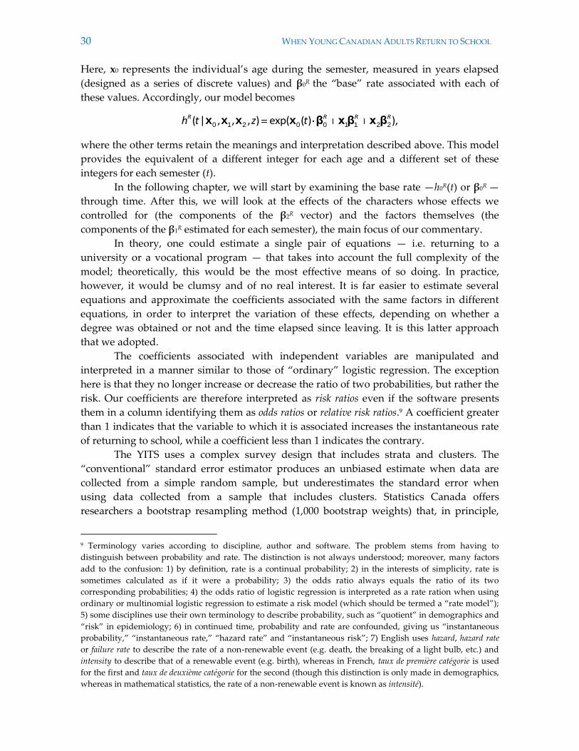
30 WHEN YOUNG CANADIAN ADULTS RETURN TO SCHOOL
Here, x0 represents the individual’s age during the semester, measured in years elapsed
(designed as a series of discrete values) and β0R the “base” rate associated with each of
these values. Accordingly, our model becomes
( | , , , ) exp( ( ) ),R R R Rh t z tx x x x β x β x β0 1 2 0 0 1 1 2 2
where the other terms retain the meanings and interpretation described above. This model
provides the equivalent of a different integer for each age and a different set of these
integers for each semester (t).
In the following chapter, we will start by examining the base rate —h0R(t) or β0R —
through time. After this, we will look at the effects of the characters whose effects we
controlled for (the components of the β2R vector) and the factors themselves (the
components of the β1R estimated for each semester), the main focus of our commentary.
In theory, one could estimate a single pair of equations — i.e. returning to a
university or a vocational program — that takes into account the full complexity of the
model; theoretically, this would be the most effective means of so doing. In practice,
however, it would be clumsy and of no real interest. It is far easier to estimate several
equations and approximate the coefficients associated with the same factors in different
equations, in order to interpret the variation of these effects, depending on whether a
degree was obtained or not and the time elapsed since leaving. It is this latter approach
that we adopted.
The coefficients associated with independent variables are manipulated and
interpreted in a manner similar to those of “ordinary” logistic regression. The exception
here is that they no longer increase or decrease the ratio of two probabilities, but rather the
risk. Our coefficients are therefore interpreted as risk ratios even if the software presents
them in a column identifying them as odds ratios or relative risk ratios.9 A coefficient greater
than 1 indicates that the variable to which it is associated increases the instantaneous rate
of returning to school, while a coefficient less than 1 indicates the contrary.
The YITS uses a complex survey design that includes strata and clusters. The
“conventional” standard error estimator produces an unbiased estimate when data are
collected from a simple random sample, but underestimates the standard error when
using data collected from a sample that includes clusters. Statistics Canada offers
researchers a bootstrap resampling method (1,000 bootstrap weights) that, in principle,
9 Terminology varies according to discipline, author and software. The problem stems from having to
distinguish between probability and rate. The distinction is not always understood; moreover, many factors
add to the confusion: 1) by definition, rate is a continual probability; 2) in the interests of simplicity, rate is
sometimes calculated as if it were a probability; 3) the odds ratio always equals the ratio of its two
corresponding probabilities; 4) the odds ratio of logistic regression is interpreted as a rate ration when using
ordinary or multinomial logistic regression to estimate a risk model (which should be termed a “rate model”);
5) some disciplines use their own terminology to describe probability, such as “quotient” in demographics and
“risk” in epidemiology; 6) in continued time, probability and rate are confounded, giving us “instantaneous
probability,” “instantaneous rate,” “hazard rate” and “instantaneous risk”; 7) English uses hazard, hazard rate
or failure rate to describe the rate of a non-renewable event (e.g. death, the breaking of a light bulb, etc.) and
intensity to describe that of a renewable event (e.g. birth), whereas in French, taux de première catégorie is used
for the first and taux de deuxième catégorie for the second (though this distinction is only made in demographics,
whereas in mathematical statistics, the rate of a non-renewable event is known as intensité).

31
allows us to obtain unbiased estimates of standard errors through re-estimation, even if
the YITS data were not collected through simple random sampling. We used this method
to calculate standard errors that are used to determine the significance level associated
with our equations’ coefficients.

32 WHEN YOUNG CANADIAN ADULTS RETURN TO SCHOOL
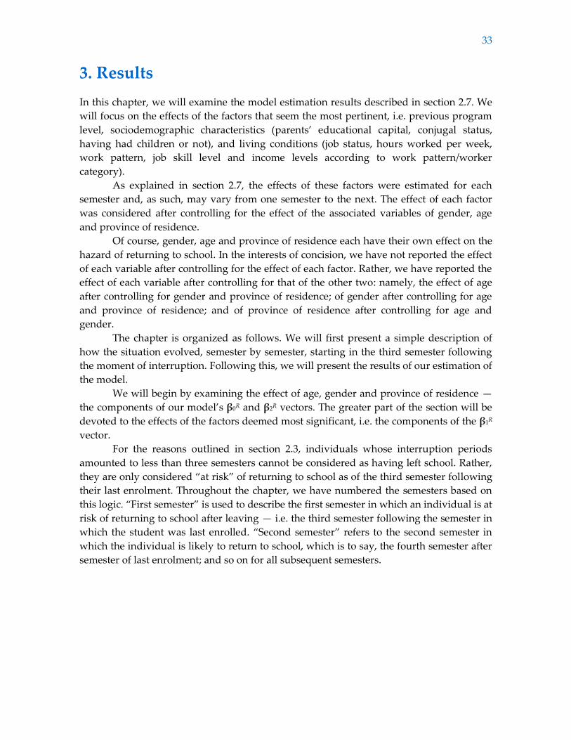
33
3. Results
In this chapter, we will examine the model estimation results described in section 2.7. We
will focus on the effects of the factors that seem the most pertinent, i.e. previous program
level, sociodemographic characteristics (parents’ educational capital, conjugal status,
having had children or not), and living conditions (job status, hours worked per week,
work pattern, job skill level and income levels according to work pattern/worker
category).
As explained in section 2.7, the effects of these factors were estimated for each
semester and, as such, may vary from one semester to the next. The effect of each factor
was considered after controlling for the effect of the associated variables of gender, age
and province of residence.
Of course, gender, age and province of residence each have their own effect on the
hazard of returning to school. In the interests of concision, we have not reported the effect
of each variable after controlling for the effect of each factor. Rather, we have reported the
effect of each variable after controlling for that of the other two: namely, the effect of age
after controlling for gender and province of residence; of gender after controlling for age
and province of residence; and of province of residence after controlling for age and
gender.
The chapter is organized as follows. We will first present a simple description of
how the situation evolved, semester by semester, starting in the third semester following
the moment of interruption. Following this, we will present the results of our estimation of
the model.
We will begin by examining the effect of age, gender and province of residence —
the components of our model’s β0R and β2R vectors. The greater part of the section will be
devoted to the effects of the factors deemed most significant, i.e. the components of the β1R
vector.
For the reasons outlined in section 2.3, individuals whose interruption periods
amounted to less than three semesters cannot be considered as having left school. Rather,
they are only considered “at risk” of returning to school as of the third semester following
their last enrolment. Throughout the chapter, we have numbered the semesters based on
this logic. “First semester” is used to describe the first semester in which an individual is at
risk of returning to school after leaving — i.e. the third semester following the semester in
which the student was last enrolled. “Second semester” refers to the second semester in
which the individual is likely to return to school, which is to say, the fourth semester after
semester of last enrolment; and so on for all subsequent semesters.
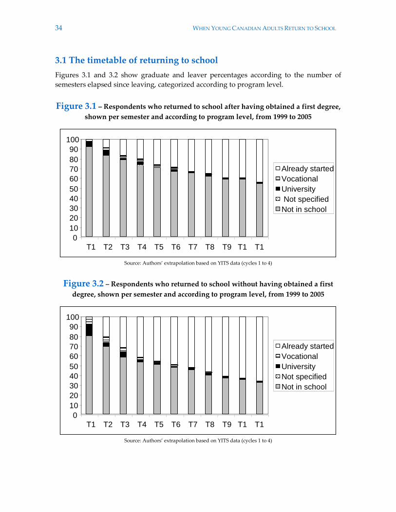
34 WHEN YOUNG CANADIAN ADULTS RETURN TO SCHOOL
3.1 The timetable of returning to school
Figures 3.1 and 3.2 show graduate and leaver percentages according to the number of
semesters elapsed since leaving, categorized according to program level.
Figure 3.1 – Respondents who returned to school after having obtained a first degree,
shown per semester and according to program level, from 1999 to 2005
0
10
20
30
40
50
60
70
80
90
100
T1 T2 T3 T4 T5 T6 T7 T8 T9 T10
T11
Already started
Vocational
University
Not specified
Not in school
Source: Authors’ extrapolation based on YITS data (cycles 1 to 4)
Figure 3.2 – Respondents who returned to school without having obtained a first
degree, shown per semester and according to program level, from 1999 to 2005
0
10
20
30
40
50
60
70
80
90
100
T1 T2 T3 T4 T5 T6 T7 T8 T9 T10
T11
Already started
Vocational
University
Not specified
Not in school
Source: Authors’ extrapolation based on YITS data (cycles 1 to 4)
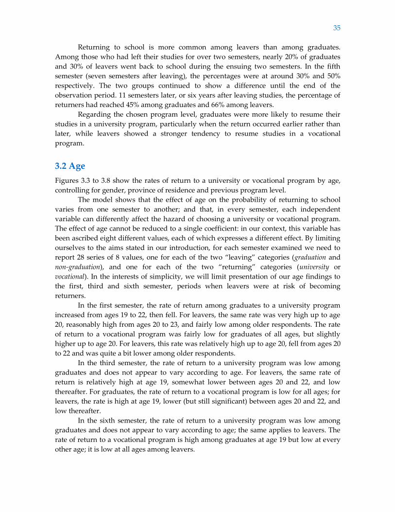
35
Returning to school is more common among leavers than among graduates.
Among those who had left their studies for over two semesters, nearly 20% of graduates
and 30% of leavers went back to school during the ensuing two semesters. In the fifth
semester (seven semesters after leaving), the percentages were at around 30% and 50%
respectively. The two groups continued to show a difference until the end of the
observation period. 11 semesters later, or six years after leaving studies, the percentage of
returners had reached 45% among graduates and 66% among leavers.
Regarding the chosen program level, graduates were more likely to resume their
studies in a university program, particularly when the return occurred earlier rather than
later, while leavers showed a stronger tendency to resume studies in a vocational
program.
3.2 Age
Figures 3.3 to 3.8 show the rates of return to a university or vocational program by age,
controlling for gender, province of residence and previous program level.
The model shows that the effect of age on the probability of returning to school
varies from one semester to another; and that, in every semester, each independent
variable can differently affect the hazard of choosing a university or vocational program.
The effect of age cannot be reduced to a single coefficient: in our context, this variable has
been ascribed eight different values, each of which expresses a different effect. By limiting
ourselves to the aims stated in our introduction, for each semester examined we need to
report 28 series of 8 values, one for each of the two “leaving” categories (graduation and
non-graduation), and one for each of the two “returning” categories (university or
vocational). In the interests of simplicity, we will limit presentation of our age findings to
the first, third and sixth semester, periods when leavers were at risk of becoming
returners.
In the first semester, the rate of return among graduates to a university program
increased from ages 19 to 22, then fell. For leavers, the same rate was very high up to age
20, reasonably high from ages 20 to 23, and fairly low among older respondents. The rate
of return to a vocational program was fairly low for graduates of all ages, but slightly
higher up to age 20. For leavers, this rate was relatively high up to age 20, fell from ages 20
to 22 and was quite a bit lower among older respondents.
In the third semester, the rate of return to a university program was low among
graduates and does not appear to vary according to age. For leavers, the same rate of
return is relatively high at age 19, somewhat lower between ages 20 and 22, and low
thereafter. For graduates, the rate of return to a vocational program is low for all ages; for
leavers, the rate is high at age 19, lower (but still significant) between ages 20 and 22, and
low thereafter.
In the sixth semester, the rate of return to a university program was low among
graduates and does not appear to vary according to age; the same applies to leavers. The
rate of return to a vocational program is high among graduates at age 19 but low at every
other age; it is low at all ages among leavers.
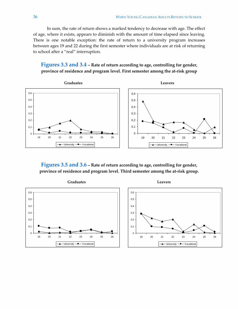
36 WHEN YOUNG CANADIAN ADULTS RETURN TO SCHOOL
In sum, the rate of return shows a marked tendency to decrease with age. The effect
of age, where it exists, appears to diminish with the amount of time elapsed since leaving.
There is one notable exception: the rate of return to a university program increases
between ages 19 and 22 during the first semester where individuals are at risk of returning
to school after a “real” interruption.
Figures 3.3 and 3.4 – Rate of return according to age, controlling for gender,
province of residence and program level. First semester among the at-risk group
Graduates Leavers
0
0,1
0,2
0,3
0,4
0,5
0,6
19 20 21 22 23 24 25 26
University Vocational
0
0,1
0,2
0,3
0,4
0,5
0,6
19 20 21 22 23 24 25 26
University Vocational
Figures 3.5 and 3.6 – Rate of return according to age, controlling for gender,
province of residence and program level. Third semester among the at-risk group.
Graduates Leavers
0
0,1
0,2
0,3
0,4
0,5
0,6
19 20 21 22 23 24 25 26
University Vocational
0
0,1
0,2
0,3
0,4
0,5
0,6
19 20 21 22 23 24 25 26
University Vocational
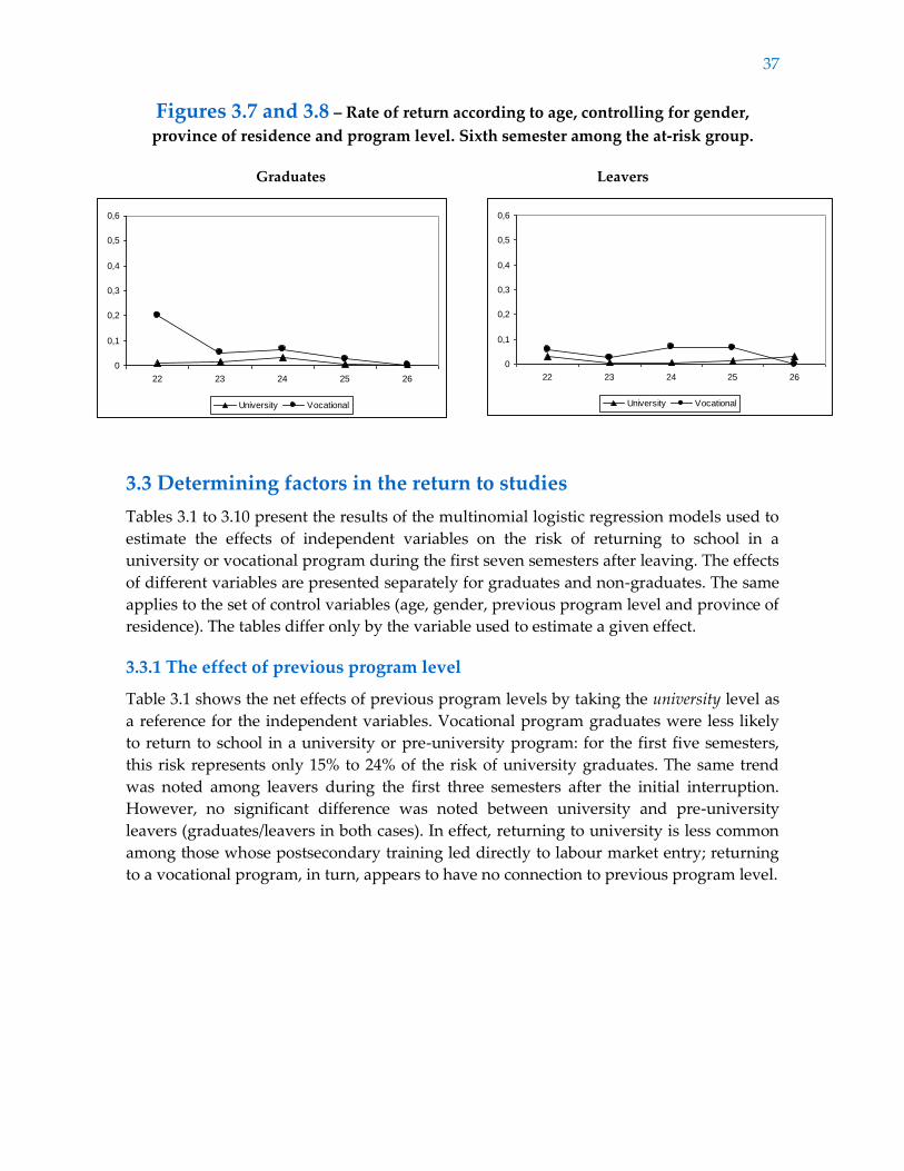
37
Figures 3.7 and 3.8 – Rate of return according to age, controlling for gender,
province of residence and program level. Sixth semester among the at-risk group.
Graduates Leavers
0
0,1
0,2
0,3
0,4
0,5
0,6
22 23 24 25 26
University Vocational
0
0,1
0,2
0,3
0,4
0,5
0,6
22 23 24 25 26
University Vocational
3.3 Determining factors in the return to studies
Tables 3.1 to 3.10 present the results of the multinomial logistic regression models used to
estimate the effects of independent variables on the risk of returning to school in a
university or vocational program during the first seven semesters after leaving. The effects
of different variables are presented separately for graduates and non-graduates. The same
applies to the set of control variables (age, gender, previous program level and province of
residence). The tables differ only by the variable used to estimate a given effect.
3.3.1 The effect of previous program level
Table 3.1 shows the net effects of previous program levels by taking the university level as
a reference for the independent variables. Vocational program graduates were less likely
to return to school in a university or pre-university program: for the first five semesters,
this risk represents only 15% to 24% of the risk of university graduates. The same trend
was noted among leavers during the first three semesters after the initial interruption.
However, no significant difference was noted between university and pre-university
leavers (graduates/leavers in both cases). In effect, returning to university is less common
among those whose postsecondary training led directly to labour market entry; returning
to a vocational program, in turn, appears to have no connection to previous program level.
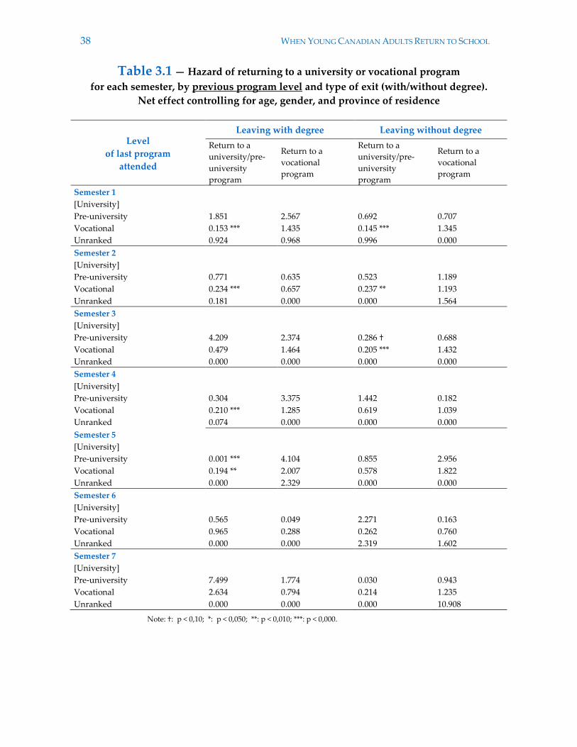
38 WHEN YOUNG CANADIAN ADULTS RETURN TO SCHOOL
Table 3.1 — Hazard of returning to a university or vocational program
for each semester, by previous program level and type of exit (with/without degree).
Net effect controlling for age, gender, and province of residence
Level
of last program
attended
Leaving with degree Leaving without degree
Return to a
university/pre-
university
program
Return to a
vocational
program
Return to a
university/pre-
university
program
Return to a
vocational
program
Semester 1
[University]
Pre-university 1.851 2.567 0.692 0.707
Vocational 0.153 *** 1.435 0.145 *** 1.345
Unranked 0.924 0.968 0.996 0.000
Semester 2
[University]
Pre-university 0.771 0.635 0.523 1.189
Vocational 0.234 *** 0.657 0.237 ** 1.193
Unranked 0.181 0.000 0.000 1.564
Semester 3
[University]
Pre-university 4.209 2.374 0.286 † 0.688
Vocational 0.479 1.464 0.205 *** 1.432
Unranked 0.000 0.000 0.000 0.000
Semester 4
[University]
Pre-university 0.304 3.375 1.442 0.182
Vocational 0.210 *** 1.285 0.619 1.039
Unranked 0.074 0.000 0.000 0.000
Semester 5
[University]
Pre-university 0.001 *** 4.104 0.855 2.956
Vocational 0.194 ** 2.007 0.578 1.822
Unranked 0.000 2.329 0.000 0.000
Semester 6
[University]
Pre-university 0.565 0.049 2.271 0.163
Vocational 0.965 0.288 0.262 0.760
Unranked 0.000 0.000 2.319 1.602
Semester 7
[University]
Pre-university 7.499 1.774 0.030 0.943
Vocational 2.634 0.794 0.214 1.235
Unranked 0.000 0.000 0.000 10.908
Note: †: p < 0,10; *: p < 0,050; **: p < 0,010; ***: p < 0,000.

39
3.3.2 The impact of socio-demographic characteristics
Table 3.2 presents the net effect of province of residence after controlling for age, gender
and previous program level. The results indicate no significant differences between the
provinces; moreover, significant differences are observed only in the first three semesters.
In the Prairies, graduates were more likely to return to school in a vocational program,
while their leaver counterparts showed a lower risk of returning to school altogether. In
Quebec, graduates were more likely to return to a university program, though this
difference disappeared with time.
Parents’ educational capital also had a significant effect on the hazard of returning
to school (Table 3.3). Graduates and leavers whose parents had attended university were
at a higher risk of returning to a university program; their risk was two to three times
higher than first-generation students. Having parents with postsecondary training also
increased the risk of returning to a vocational program after dropping out of a (first)
program. Overall, the return to school was both more likely and more rapid among youth
whose parents had university experience.
We measured the influence of family circumstances by considering conjugal status
and parenthood; our results are presented in tables 3.4 and 3.5. Living as a member of a
couple reduced the risk of undertaking studies, regardless of the manner of leaving (with
or without a degree). Entering into parenthood does not appear to have a significant effect
on the hazard of returning to school, though this is probably explained by the fact that
most births occur after the couple has formed, once most of the thresholds related to the
transition to adulthood have been crossed.
Table 3.2 — Hazard of returning to a university or vocational program
for each semester, by province of residence and type of exit (with/without degree).
Net effect controlling for age, gender, and previous program level
Province of residence
Leaving with degree Leaving without degree
Return to a
university/pre-
university program
Return to a
vocational
program
Return to a
university/pre-
university program
Return to a
vocational
program
Semester 1
[Ontario]
Maritimes 0.582 0.890 0.626 1.024
Quebec 1.547 0.251 1.359 0.871
Prairies 0.956 2.308 † 0.578 † 0.317 †
British Columbia 1.003 0.634 1.129 0.513
Semester 2
[Ontario]
Maritimes 1.333 1.041 1.444 0.761
Quebec 2.702 * 0.407 1.802 0.611
Prairies 0.851 1.150 1.322 0.651
British Columbia 0.582 1.524 2.648 1.574
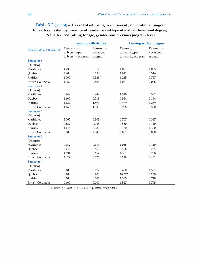
40 WHEN YOUNG CANADIAN ADULTS RETURN TO SCHOOL
Table 3.2 (cont’d)— Hazard of returning to a university or vocational program
for each semester, by province of residence and type of exit (with/without degree).
Net effect controlling for age, gender, and previous program level
Province of residence
Leaving with degree Leaving without degree
Return to a
university/pre-
university program
Return to a
vocational
program
Return to a
university/pre-
university program
Return to a
vocational
program
Semester 3
[Ontario]
Maritimes 1.435 0.312 1.091 1.065
Quebec 2.600 0.158 1.011 0.316
Prairies 1.200 0.329 ** 1.245 0.757
British Columbia 1.167 0.805 1.071 2.076
Semester 4
[Ontario]
Maritimes 0.849 0.949 1.510 0.382 †
Quebec 1.800 0.518 0.524 0.164
Prairies 1.032 1.896 0.479 1.259
British Columbia 1.060 1.049 0.978 0.580
Semester 5
[Ontario]
Maritimes 3.262 0.303 0.707 0.347
Quebec 4.882 0.165 0.550 0.140
Prairies 1.044 0.580 0.430 1.330
British Columbia 0.700 2.045 0.092 0.000
Semester 6
[Ontario]
Maritimes 0.952 0.614 1.018 0.440
Quebec 2.049 0.463 0.526 0.225
Prairies 1.531 0.654 1.301 0.798
British Columbia 7.429 0.070 0.218 0.461
Semester 7
[Ontario]
Maritimes 0.000 0.177 0.460 1.597
Quebec 0.000 0.289 14.772 0.258
Prairies 0.000 0.101 1.355 0.728
British Columbia 0.000 0.000 1.527 0.705
Note: †: p < 0.100; *: p < 0.050; **: p < 0.010 ***: p < 0.000
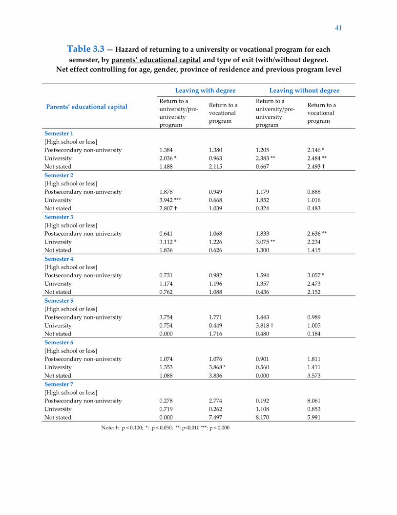
41
Table 3.3 — Hazard of returning to a university or vocational program for each
semester, by parents’ educational capital and type of exit (with/without degree).
Net effect controlling for age, gender, province of residence and previous program level
Parents’ educational capital
Leaving with degree Leaving without degree
Return to a
university/pre-
university
program
Return to a
vocational
program
Return to a
university/pre-
university
program
Return to a
vocational
program
Semester 1
[High school or less]
Postsecondary non-university 1.384 1.380 1.205 2.146 *
University 2.036 * 0.963 2.383 ** 2.484 **
Not stated 1.488 2.115 0.667 2.493 †
Semester 2
[High school or less]
Postsecondary non-university 1.878 0.949 1.179 0.888
University 3.942 *** 0.668 1.852 1.016
Not stated 2.807 † 1.039 0.324 0.483
Semester 3
[High school or less]
Postsecondary non-university 0.641 1.068 1.833 2.636 **
University 3.112 * 1.226 3.075 ** 2.234
Not stated 1.836 0.626 1.300 1.415
Semester 4
[High school or less]
Postsecondary non-university 0.731 0.982 1.594 3.057 *
University 1.174 1.196 1.357 2.473
Not stated 0.762 1.088 0.436 2.152
Semester 5
[High school or less]
Postsecondary non-university 3.754 1.771 1.443 0.989
University 0.754 0.449 3.818 † 1.005
Not stated 0.000 1.716 0.480 0.184
Semester 6
[High school or less]
Postsecondary non-university 1.074 1.076 0.901 1.811
University 1.353 3.868 * 0.560 1.411
Not stated 1.088 3.836 0.000 3.573
Semester 7
[High school or less]
Postsecondary non-university 0.278 2.774 0.192 8.061
University 0.719 0.262 1.108 0.853
Not stated 0.000 7.497 8.170 5.991
Note: †: p < 0,100; *: p < 0,050; **: p<0,010 ***: p < 0,000
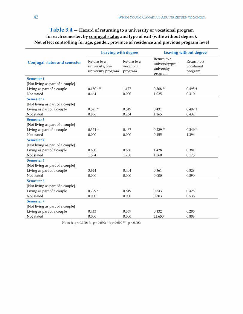
42 WHEN YOUNG CANADIAN ADULTS RETURN TO SCHOOL
Table 3.4 — Hazard of returning to a university or vocational program
for each semester, by conjugal status and type of exit (with/without degree).
Net effect controlling for age, gender, province of residence and previous program level
Conjugal status and semester
Leaving with degree Leaving without degree
Return to a
university/pre-
university program
Return to a
vocational
program
Return to a
university/pre-
university
program
Return to a
vocational
program
Semester 1
[Not living as part of a couple]
Living as part of a couple 0.180 *** 1.177 0.308 ** 0.495 †
Not stated 0.464 0.000 1.025 0.310
Semester 2
[Not living as part of a couple]
Living as part of a couple 0.525 * 0.519 0.431 0.497 †
Not stated 0.836 0.264 1.265 0.432
Semester 3
[Not living as part of a couple]
Living as part of a couple 0.374 † 0.467 0.229 ** 0.349 *
Not stated 0.000 0.000 0.455 1.396
Semester 4
[Not living as part of a couple]
Living as part of a couple 0.600 0.650 1.428 0.381
Not stated 1.594 1.258 1.860 0.175
Semester 5
[Not living as part of a couple]
Living as part of a couple 3.624 0.404 0.361 0.828
Not stated 0.000 0.000 0.000 0.890
Semester 6
[Not living as part of a couple]
Living as part of a couple 0.299 * 0.819 0.543 0.425
Not stated 0.000 0.000 0.303 0.536
Semester 7
[Not living as part of a couple]
Living as part of a couple 0.443 0.359 0.132 0.205
Not stated 0.000 0.000 22.650 0.803
Note: †: p < 0,100; *: p < 0,050; **: p<0,010 ***: p < 0,000.
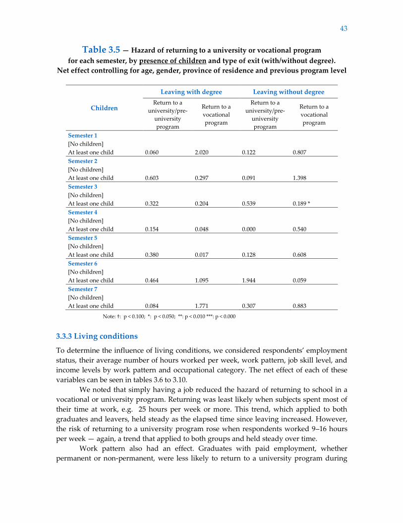
43
Table 3.5 — Hazard of returning to a university or vocational program
for each semester, by presence of children and type of exit (with/without degree).
Net effect controlling for age, gender, province of residence and previous program level
Children
Leaving with degree Leaving without degree
Return to a
university/pre-
university
program
Return to a
vocational
program
Return to a
university/pre-
university
program
Return to a
vocational
program
Semester 1
[No children]
At least one child 0.060 2.020 0.122 0.807
Semester 2
[No children]
At least one child 0.603 0.297 0.091 1.398
Semester 3
[No children]
At least one child 0.322 0.204 0.539 0.189 *
Semester 4
[No children]
At least one child 0.154 0.048 0.000 0.540
Semester 5
[No children]
At least one child 0.380 0.017 0.128 0.608
Semester 6
[No children]
At least one child 0.464 1.095 1.944 0.059
Semester 7
[No children]
At least one child 0.084 1.771 0.307 0.883
Note: †: p < 0.100; *: p < 0.050; **: p < 0.010 ***: p < 0.000
3.3.3 Living conditions
To determine the influence of living conditions, we considered respondents’ employment
status, their average number of hours worked per week, work pattern, job skill level, and
income levels by work pattern and occupational category. The net effect of each of these
variables can be seen in tables 3.6 to 3.10.
We noted that simply having a job reduced the hazard of returning to school in a
vocational or university program. Returning was least likely when subjects spent most of
their time at work, e.g. 25 hours per week or more. This trend, which applied to both
graduates and leavers, held steady as the elapsed time since leaving increased. However,
the risk of returning to a university program rose when respondents worked 9–16 hours
per week — again, a trend that applied to both groups and held steady over time.
Work pattern also had an effect. Graduates with paid employment, whether
permanent or non-permanent, were less likely to return to a university program during
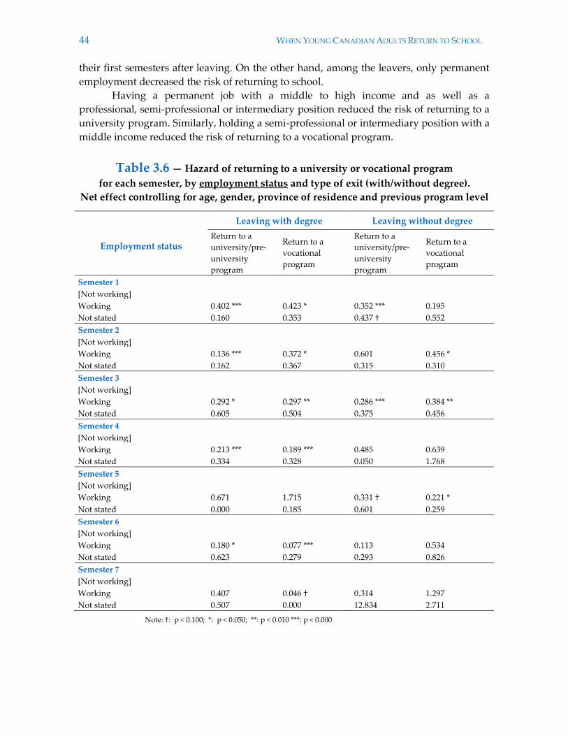
44 WHEN YOUNG CANADIAN ADULTS RETURN TO SCHOOL
their first semesters after leaving. On the other hand, among the leavers, only permanent
employment decreased the risk of returning to school.
Having a permanent job with a middle to high income and as well as a
professional, semi-professional or intermediary position reduced the risk of returning to a
university program. Similarly, holding a semi-professional or intermediary position with a
middle income reduced the risk of returning to a vocational program.
Table 3.6 — Hazard of returning to a university or vocational program
for each semester, by employment status and type of exit (with/without degree).
Net effect controlling for age, gender, province of residence and previous program level
Leaving with degree Leaving without degree
Employment status
Return to a
university/pre-
university
program
Return to a
vocational
program
Return to a
university/pre-
university
program
Return to a
vocational
program
Semester 1
[Not working]
Working 0.402 *** 0.423 * 0.352 *** 0.195
Not stated 0.160 0.353 0.437 † 0.552
Semester 2
[Not working]
Working 0.136 *** 0.372 * 0.601 0.456 *
Not stated 0.162 0.367 0.315 0.310
Semester 3
[Not working]
Working 0.292 * 0.297 ** 0.286 *** 0.384 **
Not stated 0.605 0.504 0.375 0.456
Semester 4
[Not working]
Working 0.213 *** 0.189 *** 0.485 0.639
Not stated 0.334 0.328 0.050 1.768
Semester 5
[Not working]
Working 0.671 1.715 0.331 † 0.221 *
Not stated 0.000 0.185 0.601 0.259
Semester 6
[Not working]
Working 0.180 * 0.077 *** 0.113 0.534
Not stated 0.623 0.279 0.293 0.826
Semester 7
[Not working]
Working 0.407 0.046 † 0.314 1.297
Not stated 0.507 0.000 12.834 2.711
Note: †: p < 0.100; *: p < 0.050; **: p < 0.010 ***: p < 0.000
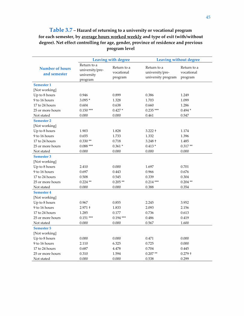
45
Table 3.7 – Hazard of returning to a university or vocational program
for each semester, by average hours worked weekly and type of exit (with/without
degree). Net effect controlling for age, gender, province of residence and previous
program level
Number of hours
and semester
Leaving with degree Leaving without degree
Return to a
university/pre-
university
program
Return to a
vocational
program
Return to a
university/pre-
university program
Return to a
vocational
program
Semester 1
[Not working]
Up to 8 hours 0.946 0.899 0.386 1.249
9 to 16 hours 3.095 * 1.328 1.703 1.099
17 to 24 hours 0.604 0.638 0.660 1.286
25 or more hours 0.150 *** 0.427 * 0.235 *** 0.494 *
Not stated 0.000 0.000 0.461 0.547
Semester 2
[Not working]
Up to 8 hours 1.903 1.828 3.222 † 1.174
9 to 16 hours 0.655 1.733 1.332 1.396
17 to 24 hours 0.330 ** 0.718 3.248 † 1.485
25 or more hours 0.088 *** 0.361 * 0.413 * 0.317 **
Not stated 0.000 0.000 0.000 0.000
Semester 3
[Not working]
Up to 8 hours 2.410 0.000 1.697 0.701
9 to 16 hours 0.697 0.443 0.966 0.676
17 to 24 hours 0.508 0.545 0.339 0.304
25 or more hours 0.224 ** 0.205 ** 0.214 *** 0.204 **
Not stated 0.000 0.000 0.388 0.354
Semester 4
[Not working]
Up to 8 hours 0.967 0.855 2.245 3.952
9 to 16 hours 2.971 † 1.833 2.093 2.156
17 to 24 hours 1.285 0.177 0.736 0.613
25 or more hours 0.151 *** 0.194 *** 0.486 0.419
Not stated 0.000 0.000 0.567 1.600
Semester 5
[Not working]
Up to 8 hours 0.000 0.000 0.471 0.000
9 to 16 hours 2.110 6.325 0.725 0.000
17 to 24 hours 0.687 4.478 0.704 0.445
25 or more hours 0.310 1.594 0.207 ** 0.279 †
Not stated 0.000 0.000 0.538 0.299
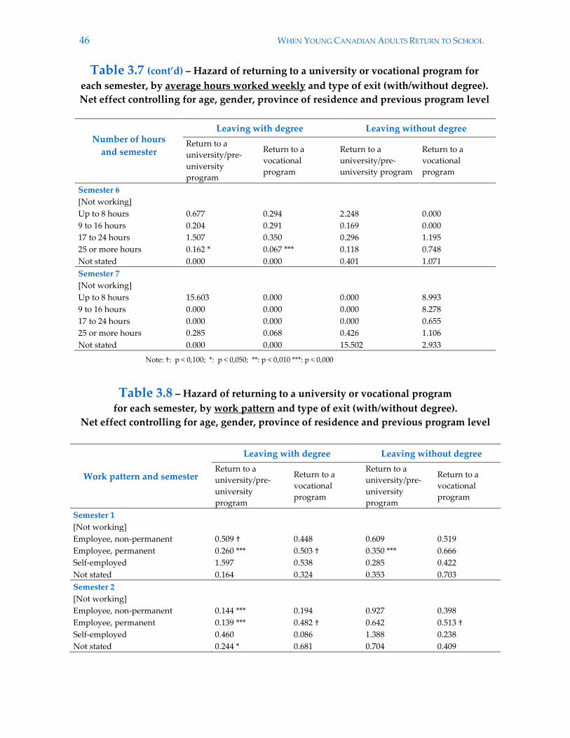
46 WHEN YOUNG CANADIAN ADULTS RETURN TO SCHOOL
Table 3.7 (cont’d) – Hazard of returning to a university or vocational program for
each semester, by average hours worked weekly and type of exit (with/without degree).
Net effect controlling for age, gender, province of residence and previous program level
Number of hours
and semester
Leaving with degree Leaving without degree
Return to a
university/pre-
university
program
Return to a
vocational
program
Return to a
university/pre-
university program
Return to a
vocational
program
Semester 6
[Not working]
Up to 8 hours 0.677 0.294 2.248 0.000
9 to 16 hours 0.204 0.291 0.169 0.000
17 to 24 hours 1.507 0.350 0.296 1.195
25 or more hours 0.162 * 0.067 *** 0.118 0.748
Not stated 0.000 0.000 0.401 1.071
Semester 7
[Not working]
Up to 8 hours 15.603 0.000 0.000 8.993
9 to 16 hours 0.000 0.000 0.000 8.278
17 to 24 hours 0.000 0.000 0.000 0.655
25 or more hours 0.285 0.068 0.426 1.106
Not stated 0.000 0.000 15.502 2.933
Note: †: p < 0,100; *: p < 0,050; **: p < 0,010 ***: p < 0,000
Table 3.8 – Hazard of returning to a university or vocational program
for each semester, by work pattern and type of exit (with/without degree).
Net effect controlling for age, gender, province of residence and previous program level
Work pattern and semester
Leaving with degree Leaving without degree
Return to a
university/pre-
university
program
Return to a
vocational
program
Return to a
university/pre-
university
program
Return to a
vocational
program
Semester 1
[Not working]
Employee, non-permanent 0.509 † 0.448 0.609 0.519
Employee, permanent 0.260 *** 0.503 † 0.350 *** 0.666
Self-employed 1.597 0.538 0.285 0.422
Not stated 0.164 0.324 0.353 0.703
Semester 2
[Not working]
Employee, non-permanent 0.144 *** 0.194 0.927 0.398
Employee, permanent 0.139 *** 0.482 † 0.642 0.513 †
Self-employed 0.460 0.086 1.388 0.238
Not stated 0.244 * 0.681 0.704 0.409
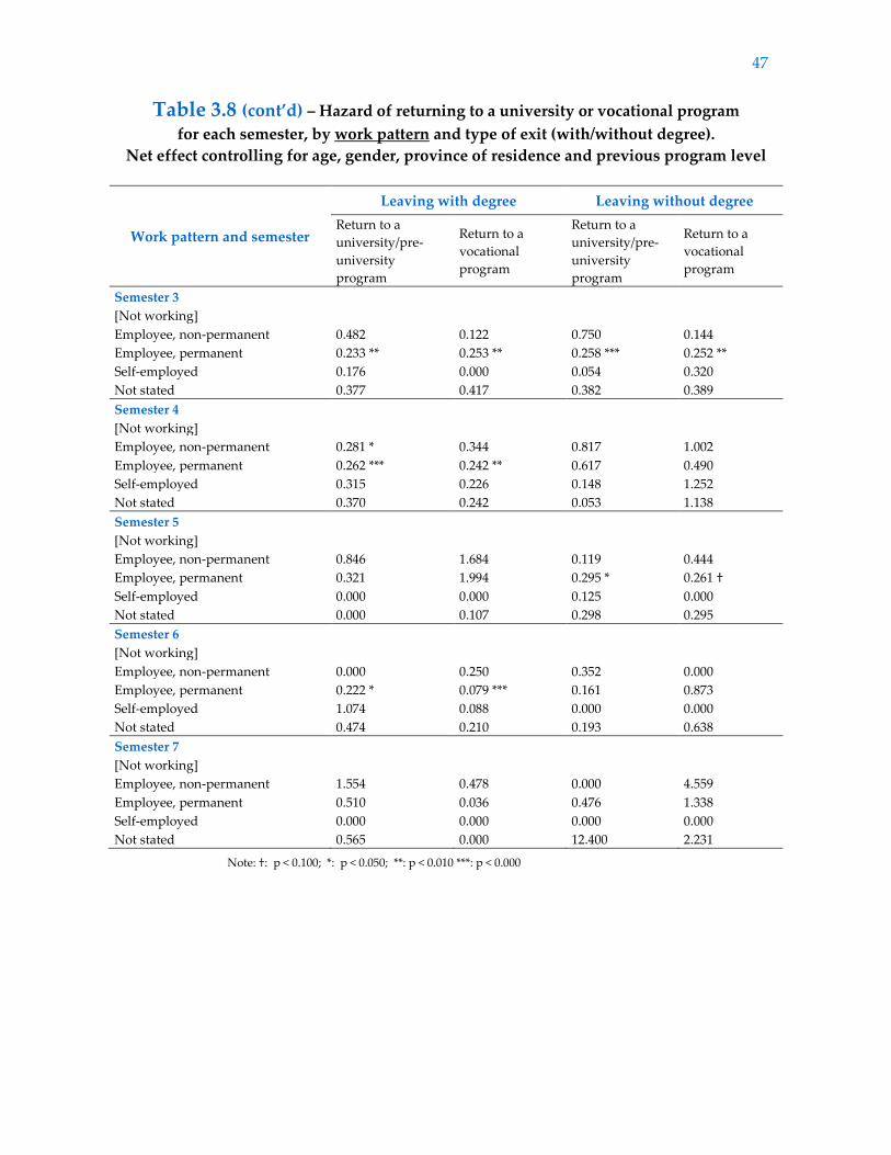
47
Table 3.8 (cont’d) – Hazard of returning to a university or vocational program
for each semester, by work pattern and type of exit (with/without degree).
Net effect controlling for age, gender, province of residence and previous program level
Work pattern and semester
Leaving with degree Leaving without degree
Return to a
university/pre-
university
program
Return to a
vocational
program
Return to a
university/pre-
university
program
Return to a
vocational
program
Semester 3
[Not working]
Employee, non-permanent 0.482 0.122 0.750 0.144
Employee, permanent 0.233 ** 0.253 ** 0.258 *** 0.252 **
Self-employed 0.176 0.000 0.054 0.320
Not stated 0.377 0.417 0.382 0.389
Semester 4
[Not working]
Employee, non-permanent 0.281 * 0.344 0.817 1.002
Employee, permanent 0.262 *** 0.242 ** 0.617 0.490
Self-employed 0.315 0.226 0.148 1.252
Not stated 0.370 0.242 0.053 1.138
Semester 5
[Not working]
Employee, non-permanent 0.846 1.684 0.119 0.444
Employee, permanent 0.321 1.994 0.295 * 0.261 †
Self-employed 0.000 0.000 0.125 0.000
Not stated 0.000 0.107 0.298 0.295
Semester 6
[Not working]
Employee, non-permanent 0.000 0.250 0.352 0.000
Employee, permanent 0.222 * 0.079 *** 0.161 0.873
Self-employed 1.074 0.088 0.000 0.000
Not stated 0.474 0.210 0.193 0.638
Semester 7
[Not working]
Employee, non-permanent 1.554 0.478 0.000 4.559
Employee, permanent 0.510 0.036 0.476 1.338
Self-employed 0.000 0.000 0.000 0.000
Not stated 0.565 0.000 12.400 2.231
Note: †: p < 0.100; *: p < 0.050; **: p < 0.010 ***: p < 0.000
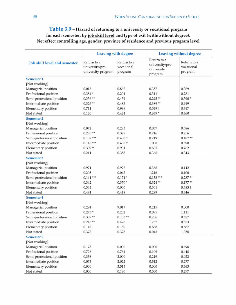
48 WHEN YOUNG CANADIAN ADULTS RETURN TO SCHOOL
Table 3.9 – Hazard of returning to a university or vocational program
for each semester, by job skill level and type of exit (with/without degree).
Net effect controlling age, gender, province of residence and previous program level
Job skill level and semester
Leaving with degree Leaving without degree
Return to a
university/pre-
university program
Return to a
vocational
program
Return to a
university/pre-
university
program
Return to a
vocational
program
Semester 1
[Not working]
Managerial position 0.018 0.867 0.357 0.369
Professional position 0.384 * 0.201 0.311 0.281
Semi-professional position 0.336 ** 0.439 0.295 ** 0.390 *
Intermediate position 0.325 ** 0.485 0.389 ** 0.919
Elementary position 0.711 0.999 0.529 † 0.617
Not stated 0.120 0.424 0.369 * 0.460
Semester 2
[Not working]
Managerial position 0.072 0.283 0.037 0.386
Professional position 0.285 ** 0.327 0.716 0.256
Semi-professional position 0.107 *** 0.430 † 0.719 0.187 **
Intermediate position 0.118 *** 0.435 † 1.008 0.590
Elementary position 0.309 † 0.931 0.635 0.762
Not stated 0.211 0.358 0.366 0.343
Semester 3
[Not working]
Managerial position 0.971 0.927 0.368 0.142
Professional position 0.205 0.043 1.216 0.100
Semi-professional position 0.141 *** 0.171 * 0.158 *** 0.287 *
Intermediate position 0.342 0.370 * 0.324 ** 0.177 **
Elementary position 0.344 0.000 0.301 0.383 †
Not stated 0.481 0.418 0.299 0.346
Semester 4
[Not working]
Managerial position 0.294 9.017 0.215 0.000
Professional position 0.273 * 0.232 0.095 1.111
Semi-professional position 0.307 ** 0.103 ** 0.256 0.627
Intermediate position 0.245 ** 0.478 1.257 0.573
Elementary position 0.113 0.160 0.668 0.587
Not stated 0.373 0.378 0.043 1.358
Semester 5
[Not working]
Managerial position 0.173 0.000 0.000 0.496
Professional position 0.726 0.764 0.109 0.448
Semi-professional position 0.356 2.000 0.219 0.022
Intermediate position 0.073 2.022 0.512 0.277
Elementary position 0.000 3.515 0.000 0.663
Not stated 0.000 0.180 0.500 0.297
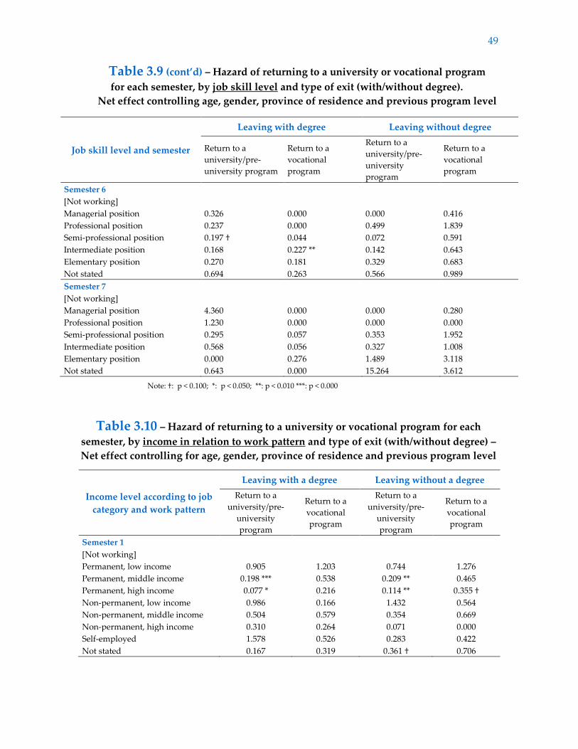
49
Table 3.9 (cont’d) – Hazard of returning to a university or vocational program
for each semester, by job skill level and type of exit (with/without degree).
Net effect controlling age, gender, province of residence and previous program level
Job skill level and semester
Leaving with degree Leaving without degree
Return to a
university/pre-
university program
Return to a
vocational
program
Return to a
university/pre-
university
program
Return to a
vocational
program
Semester 6
[Not working]
Managerial position 0.326 0.000 0.000 0.416
Professional position 0.237 0.000 0.499 1.839
Semi-professional position 0.197 † 0.044 0.072 0.591
Intermediate position 0.168 0.227 ** 0.142 0.643
Elementary position 0.270 0.181 0.329 0.683
Not stated 0.694 0.263 0.566 0.989
Semester 7
[Not working]
Managerial position 4.360 0.000 0.000 0.280
Professional position 1.230 0.000 0.000 0.000
Semi-professional position 0.295 0.057 0.353 1.952
Intermediate position 0.568 0.056 0.327 1.008
Elementary position 0.000 0.276 1.489 3.118
Not stated 0.643 0.000 15.264 3.612
Note: †: p < 0.100; *: p < 0.050; **: p < 0.010 ***: p < 0.000
Table 3.10 – Hazard of returning to a university or vocational program for each
semester, by income in relation to work pattern and type of exit (with/without degree) –
Net effect controlling for age, gender, province of residence and previous program level
Income level according to job
category and work pattern
Leaving with a degree Leaving without a degree
Return to a
university/pre-
university
program
Return to a
vocational
program
Return to a
university/pre-
university
program
Return to a
vocational
program
Semester 1
[Not working]
Permanent, low income 0.905 1.203 0.744 1.276
Permanent, middle income 0.198 *** 0.538 0.209 ** 0.465
Permanent, high income 0.077 * 0.216 0.114 ** 0.355 †
Non-permanent, low income 0.986 0.166 1.432 0.564
Non-permanent, middle income 0.504 0.579 0.354 0.669
Non-permanent, high income 0.310 0.264 0.071 0.000
Self-employed 1.578 0.526 0.283 0.422
Not stated 0.167 0.319 0.361 † 0.706
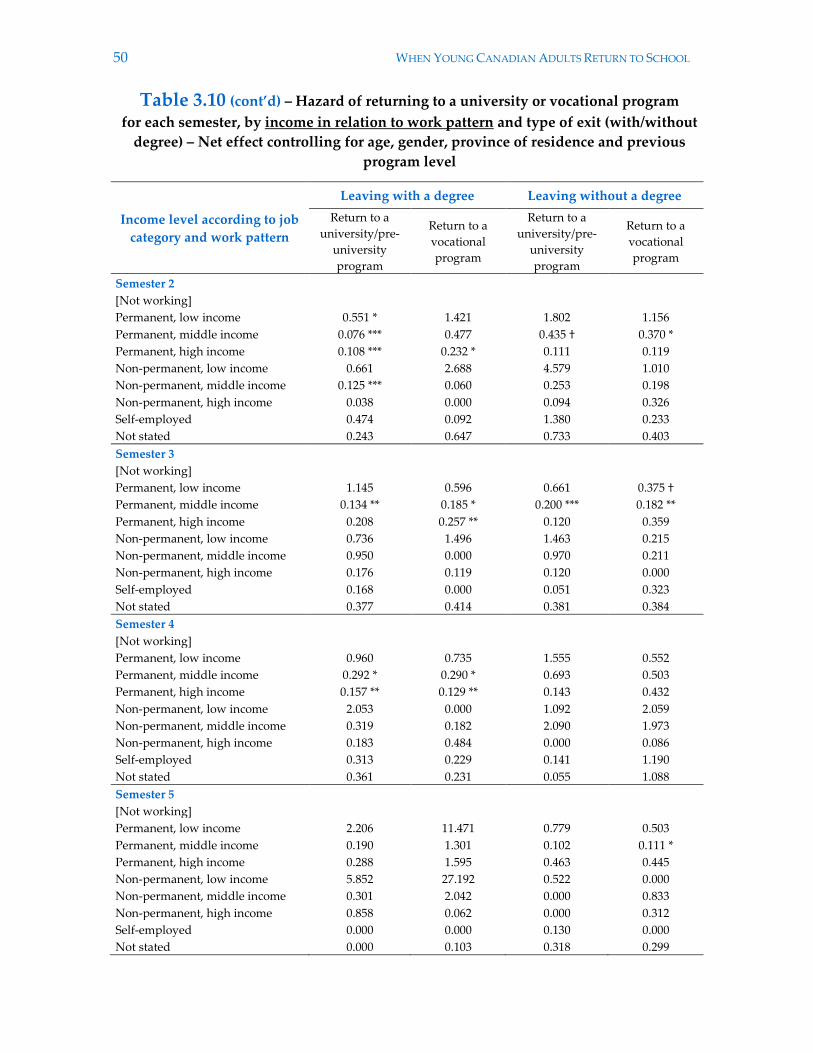
50 WHEN YOUNG CANADIAN ADULTS RETURN TO SCHOOL
Table 3.10 (cont’d) – Hazard of returning to a university or vocational program
for each semester, by income in relation to work pattern and type of exit (with/without
degree) – Net effect controlling for age, gender, province of residence and previous
program level
Income level according to job
category and work pattern
Leaving with a degree Leaving without a degree
Return to a
university/pre-
university
program
Return to a
vocational
program
Return to a
university/pre-
university
program
Return to a
vocational
program
Semester 2
[Not working]
Permanent, low income 0.551 * 1.421 1.802 1.156
Permanent, middle income 0.076 *** 0.477 0.435 † 0.370 *
Permanent, high income 0.108 *** 0.232 * 0.111 0.119
Non-permanent, low income 0.661 2.688 4.579 1.010
Non-permanent, middle income 0.125 *** 0.060 0.253 0.198
Non-permanent, high income 0.038 0.000 0.094 0.326
Self-employed 0.474 0.092 1.380 0.233
Not stated 0.243 0.647 0.733 0.403
Semester 3
[Not working]
Permanent, low income 1.145 0.596 0.661 0.375 †
Permanent, middle income 0.134 ** 0.185 * 0.200 *** 0.182 **
Permanent, high income 0.208 0.257 ** 0.120 0.359
Non-permanent, low income 0.736 1.496 1.463 0.215
Non-permanent, middle income 0.950 0.000 0.970 0.211
Non-permanent, high income 0.176 0.119 0.120 0.000
Self-employed 0.168 0.000 0.051 0.323
Not stated 0.377 0.414 0.381 0.384
Semester 4
[Not working]
Permanent, low income 0.960 0.735 1.555 0.552
Permanent, middle income 0.292 * 0.290 * 0.693 0.503
Permanent, high income 0.157 ** 0.129 ** 0.143 0.432
Non-permanent, low income 2.053 0.000 1.092 2.059
Non-permanent, middle income 0.319 0.182 2.090 1.973
Non-permanent, high income 0.183 0.484 0.000 0.086
Self-employed 0.313 0.229 0.141 1.190
Not stated 0.361 0.231 0.055 1.088
Semester 5
[Not working]
Permanent, low income 2.206 11.471 0.779 0.503
Permanent, middle income 0.190 1.301 0.102 0.111 *
Permanent, high income 0.288 1.595 0.463 0.445
Non-permanent, low income 5.852 27.192 0.522 0.000
Non-permanent, middle income 0.301 2.042 0.000 0.833
Non-permanent, high income 0.858 0.062 0.000 0.312
Self-employed 0.000 0.000 0.130 0.000
Not stated 0.000 0.103 0.318 0.299
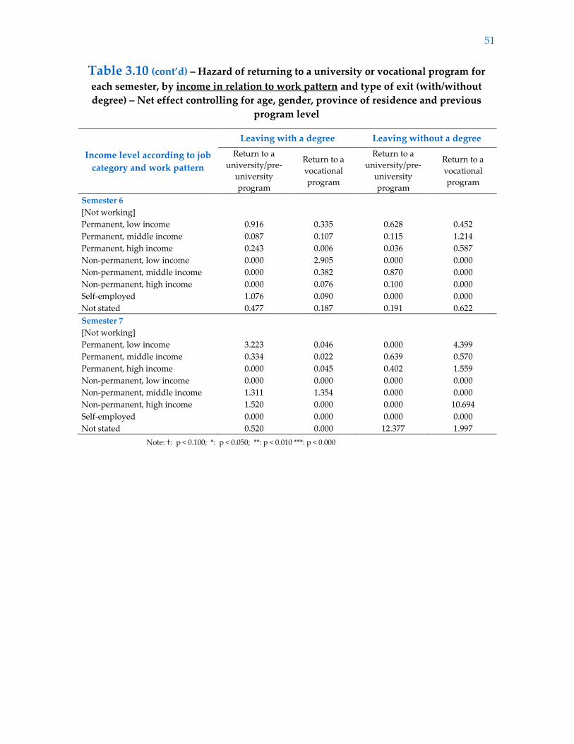
51
Table 3.10 (cont’d) – Hazard of returning to a university or vocational program for
each semester, by income in relation to work pattern and type of exit (with/without
degree) – Net effect controlling for age, gender, province of residence and previous
program level
Income level according to job
category and work pattern
Leaving with a degree Leaving without a degree
Return to a
university/pre-
university
program
Return to a
vocational
program
Return to a
university/pre-
university
program
Return to a
vocational
program
Semester 6
[Not working]
Permanent, low income 0.916 0.335 0.628 0.452
Permanent, middle income 0.087 0.107 0.115 1.214
Permanent, high income 0.243 0.006 0.036 0.587
Non-permanent, low income 0.000 2.905 0.000 0.000
Non-permanent, middle income 0.000 0.382 0.870 0.000
Non-permanent, high income 0.000 0.076 0.100 0.000
Self-employed 1.076 0.090 0.000 0.000
Not stated 0.477 0.187 0.191 0.622
Semester 7
[Not working]
Permanent, low income 3.223 0.046 0.000 4.399
Permanent, middle income 0.334 0.022 0.639 0.570
Permanent, high income 0.000 0.045 0.402 1.559
Non-permanent, low income 0.000 0.000 0.000 0.000
Non-permanent, middle income 1.311 1.354 0.000 0.000
Non-permanent, high income 1.520 0.000 0.000 10.694
Self-employed 0.000 0.000 0.000 0.000
Not stated 0.520 0.000 12.377 1.997
Note: †: p < 0.100; *: p < 0.050; **: p < 0.010 ***: p < 0.000

52 WHEN YOUNG CANADIAN ADULTS RETURN TO SCHOOL
53
Conclusion
This study aimed to understand the phenomenon of the return to postsecondary education
among young adults who had either left school after graduation or otherwise withdrawn
from their program. Specifically, we wanted to know more about the pace at which adults
returned to school, the factors that promoted or hindered the return and the influence of
variables linked to previous education, socio-demographic characteristics and living
conditions. Two modes were identified: returning to a university/pre-university program
and returning to a vocational program. We examined these modes separately, using data
from the Youth in Transition Survey (YITS) gathered from youth aged 18-20 years at the
start of the first YITS cycle.
We considered an individual to have “left” school when at least two semesters had
passed without that individual being registered in a postsecondary program. For our
purposes, the interruption needed to be of a certain length, since some breaks can stem
from administrative constraints rather than from personal choice. For example, failure to
enrol during the summer semester could be due the unavailability of courses rather than
to any individual decision.
The results showed that returning to school can vary significantly depending on
the time elapsed since leaving. Most who left (whether through graduation or
interruption) were likely to return between the first and third semester during the period
when they were considered “at risk” of returning to school — i.e. between the third and
the fifth semester following the semester preceding the interruption. Thus, a preliminary
finding is that returns are most likely in the two semesters following the cessation of
studies; the longer the interruption, the less likely the return.
The second finding is that returning to school is significantly influenced by
previous schooling. Youth who left school without obtaining their degree return in greater
numbers than graduates. Returns are also more common, generally speaking, among those
who were previously enrolled in a university or pre-university program. Among them,
graduates were more likely to re-enrol in a university or pre-university program, while
leavers (those who left their programs without obtaining a degree) were as likely to enter a
vocational as a university program.
The third finding is that there exists a significant relationship between an
individual’s demographic characteristics, his or her living conditions and the decision to
return to school. Table 3.11 lists the variables that influence the return to school by type of
exit and type of program.
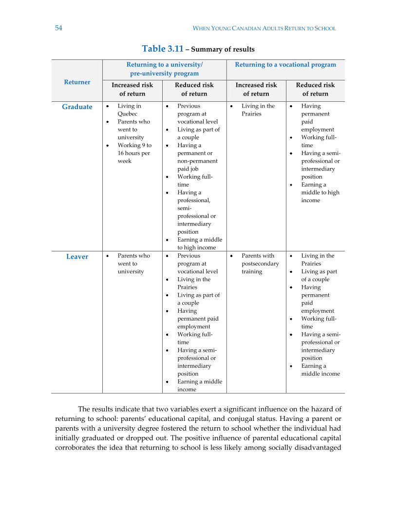
54 WHEN YOUNG CANADIAN ADULTS RETURN TO SCHOOL
Table 3.11 – Summary of results
Returner
Returning to a university/
pre-university program
Returning to a vocational program
Increased risk
of return
Reduced risk
of return
Increased risk
of return
Reduced risk
of return
Graduate Living in
Quebec
Parents who
went to
university
Working 9 to
16 hours per
week
Previous
program at
vocational level
Living as part of
a couple
Having a
permanent or
non-permanent
paid job
Working full-
time
Having a
professional,
semi-
professional or
intermediary
position
Earning a middle
to high income
Living in the
Prairies
Having
permanent
paid
employment
Working full-
time
Having a semi-
professional or
intermediary
position
Earning a
middle to high
income
Leaver Parents who
went to
university
Previous
program at
vocational level
Living in the
Prairies
Living as part of
a couple
Having
permanent paid
employment
Working full-
time
Having a semi-
professional or
intermediary
position
Earning a middle
income
Parents with
postsecondary
training
Living in the
Prairies
Living as part
of a couple
Having
permanent
paid
employment
Working full-
time
Having a semi-
professional or
intermediary
position
Earning a
middle income
The results indicate that two variables exert a significant influence on the hazard of
returning to school: parents’ educational capital, and conjugal status. Having a parent or
parents with a university degree fostered the return to school whether the individual had
initially graduated or dropped out. The positive influence of parental educational capital
corroborates the idea that returning to school is less likely among socially disadvantaged
55
groups, who were also more willing to interrupt their studies (Marcus, 1986). Living with
a partner also reduces the hazard of returning to school.
Secondly, as regards occupation and living conditions, being employed during the
interruption period reduced the probability of returning, though it rather depended on
type of employment. Indeed, the results indicate a significant relationship between job
duration, wages and the number of hours worked per week. Specifically, those who had
comparatively good working conditions — i.e. a relatively well-paid permanent job — as
well as those working 25 hours or more per week were less likely to return to school, a
finding supported by previous studies, including that of Marcus (1986). One could argue
that returning to school is associated with the aim of acquiring additional human capital to
increase the chances of accessing a desired job or improved working conditions.
Lastly, a number of differences were noted between the provinces. Among
university graduates, the rate of returning to school was higher in Quebec, while resuming
studies in a vocational program is higher in the Prairies.
The significance of our study bears on two main aspects. The first is that, from a
purely descriptive standpoint, it underscores the growing numbers of adult returners. In
this respect, returns are doubly advantaged in that they achieve complementary
objectives: they enhance the democratization of education, and they enable adults to
update their knowledge and skills in key labour market sectors.
Secondly, in highlighting the complexity and transformation of today’s educational
pathways, the study alerts policy makers and administrators to the need to consider new
contingents of adult students when developing educational policies and vocational
spheres.
However, our findings must be qualified, since the study is limited to a sample of
young adults aged 24–26, whereas we know that older adults also return to school.
Kamanzi et al. (2009), using data from the ICOPE, showed that 45% of the students
registered in the Université du Québec network were aged 26 and over. Moreover, the
YITS covered a relatively short period. In other respects, due to lack of data, the study was
limited in its ability to profile student returners, and unable to address the reasons that
propel adults to return to school after an interruption. To better understand the
complexity of the phenomenon, future research should expand the analysis of older adults
(26 and up) to cover a longer period and investigate their motivations for returning to
school.

56 WHEN YOUNG CANADIAN ADULTS RETURN TO SCHOOL

57
Bibliography
Apt Harper, P. 1978. “Adult learners and higher education: factors influencing participation or
nonparticipation decisions.” Alternative Higher Education (3) 1: 3-11.
Berger, P. and T. Luckmann. 1992. La construction sociale de la réalité. Paris, Méridiens
Klincksieck.
Brzinsky-Fay, Christian, Ulrich Kohler and Magdalena Luniak. 2006. "Sequence Analysis with
Stata.” Stata Journal (4): 435-460.
Clark, Warren. 1999. “University graduates at college”. Canadian Social Trends, Autumn 1999.
Statistics Canada — Catalogue No. 11-008.
[ http://www.statcan.gc.ca/pub/11-008-x/1999002/article/4659-eng.pdf ]
Cooksey, E. C. and R. R. Rindfuss. 1994. “Prior activities and progress in MBA programs.”
Research in Higher Education (35) 6: 647-668.
Davey, J. A. and A. Jamieson. 2003. “Against the Odds: Pathways of Early School Leavers into
University Education: Evidence from England and New Zealand.” International Journal of
Lifelong Education 22 (3): 266-80.
Davies, R. and P. Elias. Dropping Out: A Study of Early Leavers From Higher Education. Norwich,
UK, Institute for Employment Research.
Doray, Pierre and Pascal Mayrand. 2001. “Une innovation institutionnelle à l’Université : la
participation des adultes.” Talk given at the Colloque de l’ACDEAULF, University of Ottawa.
Galland, O. 1991. Sociologie de la jeunesse. L’entrée dans la vie. Paris, Armand Colin.
Goldberg, Barbara J. 1985. “Perceived Effects of a Financial Aid Scholarship on Returning
Women Students.” Research Report No. 7-85. University of Maryland.
Hango, D. (2007). “Taking time off between high school and postsecondary education:
Determinants and early labour market outcomes”. Education Matters, vol. 4, no. 5
[ http://www.statcan.gc.ca/pub/81-004-x/2007005/article/10501-eng.htm ]
Hearn, J. C. 1992. “Emerging variations in postsecondary attendance patterns: An investigation
of part-time, delayed, and non-degree enrolment.” Research in Higher Education (33) 6: 657-687.
Horn, L. J. and C. D. Carroll. 1998. Stopouts or Stayouts? Undergraduates who leave College in their
First Year. National Center for Education Statistics, U.S. Department of Education, Office of
Educational Research and Improvement.
Human Resources and Skills Development Canada. 2006. Introduction to Edition 2001 of the
National Occupational Classification (NOC).
[ http://www5.hrsdc.gc.ca/NOC/English/NOC/2006/Introduction.aspx ]

58 WHEN YOUNG CANADIAN ADULTS RETURN TO SCHOOL
Kamanzi, Pierre Canisius et al. (2010). Academic Persistence Among First-Generation Canadian
University Students. (Projet Transitions, Research Paper 9). Montreal, CIRST.
[ http://www.cirst.uqam.ca/transitions ]
Kwong, T. M., Y. F. Mok and Y. L. Kwong. 1997. “Social Factors and Adult Learners'
Motivations in Re-entering Higher Education.” International Journal of Lifelong Education 16 (6):
518-34.
Lambert, M., K. Zeman et al. 2004. Who pursues postsecondary education,who leaves and why:
Results from the Youth in Transition Survey. Ottawa: Statistics Canada.
[ http://www.statcan.gc.ca/pub/81-595-m/81-595-m2004026-eng.pdf ]
Lee, Marcia M. 1996. “Student retention survey: why students did not return, spring semester
1994.” Westchester Community College, Valhalla, NY.
Leclerc-Olive, M. 1993. Le dire de l’événement biographique. Doctoral thesis, Université des
sciences et technologies de Lille.
Malloch, D. C. and D. C. Montgomery. 1996. “Variation in characteristics among adult
students.” Continuing Higher Education Review (60) 1: 42-53.
Marcus, Richard D. 1986. “Earnings and the Decision to Return to School.” Economics of
Education Review (5) 3: 309-317.
Ouellette, Raymond. 2009. Les statistiques de l’éducation. Enseignement primaire, secondaire,
collégial et universitaire. Québec: Gouvernement du Québec, Ministère de l’éducation du loisir et
du sport, Secteur de l'information, des communications et de l'administration.
Shaienks, D., Gluszynski, T., and Bayard, J. (2008). Postsecondary Education – Participation and
Dropping Out: Differences Across University, College and Other Types of Postsecondary Institutions.
Culture, Tourism and the Centre for Education Statistics Division. Ottawa: Statistics Canada
and Human Resources and Social Development Canada.
[ http://www.statcan.gc.ca/pub/81-595-m/81-595-m2008070-eng.pdf ]
Smart, J. C and E. T Pascarella. 1987. “Influences on the Intention to Reenter Higher
Education.” The journal of Higher Education (58) 3: 306-322.
Statistics Canada. 2007. Youth in Transition Survey (YITS), Cohort B - 24 to 26 year-olds - Cycle 4
User Guide.
Thomas, Wayne. 2001. “The Decision to Return to Full-time Education.” Education Economics (
9) 1: 37-51.
Tomkowicz, J. and T. Bushnik. 2003. Who Goes to Post-secondary Education and When: Pathways
Chosen by 20 Year-olds. Culture, Tourism and the Centre for Education Statistics: Research
Papers. Ottawa: Statistics Canada.
[ http://www.statcan.gc.ca/pub/81-595-m/81-595-m2003006-eng.pdf ] .
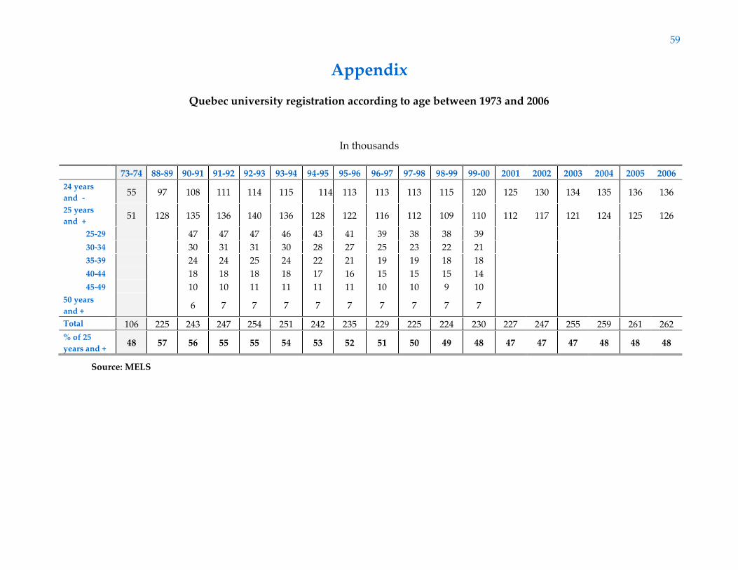
59
Appendix
Quebec university registration according to age between 1973 and 2006
In thousands
73-74 88-89 90-91 91-92 92-93 93-94 94-95 95-96 96-97 97-98 98-99 99-00 2001 2002 2003 2004 2005 2006
24 years
and -
55 97 108 111 114 115 114 113 113 113 115 120 125 130 134 135 136 136
25 years
and +
51 128 135 136 140 136 128 122 116 112 109 110 112 117 121 124 125 126
25-29 47 47 47 46 43 41 39 38 38 39
30-34 30 31 31 30 28 27 25 23 22 21
35-39 24 24 25 24 22 21 19 19 18 18
40-44 18 18 18 18 17 16 15 15 15 14
45-49 10 10 11 11 11 11 10 10 9 10
50 years
and +
6 7 7 7 7 7 7 7 7 7
Total 106 225 243 247 254 251 242 235 229 225 224 230 227 247 255 259 261 262
% of 25
years and +
48 57 56 55 55 54 53 52 51 50 49 48 47 47 47 48 48 48
Source: MELS