RESEARCH

Not All Roads Lead to Rome: Pitch Representation and Model Architecture for Automatic Harmonic AnalysisGianluca Micchi*, Mark Gotham† and Mathieu Giraud*

Automatic harmonic analysis has been an enduring focus of the MIR community, and has enjoyed a particularly vigorous revival of interest in the machine-learning age. We focus here on the specific case of Roman numeral analysis which, by virtue of requiring key/functional information in addition to chords, may be viewed as an acutely challenging use case.

We report on three main developments. First, we provide a new meta-corpus bringing together all existing Roman numeral analysis datasets; this offers greater scale and diversity, not only of the music represented, but also of human analytical viewpoints. Second, we examine best practices in the encoding of pitch, time, and harmony for machine learning tasks. The main contribution here is the introduction of full pitch spelling to such a system, an absolute must for the comprehensive study of musical harmony. Third, we devised and tested several neural network architectures and compared their relative accuracy. In the best-performing of these models, convolutional layers gather the local information needed to analyse the chord at a given moment while a recurrent part learns longer-range harmonic progressions.

Altogether, our best representation and architecture produce a small but significant improvement on overall accuracy while simultaneously integrating full pitch spelling. This enables the system to retain important information from the musical sources and provide more meaningful predictions for any new input.

Keywords: Roman numeral analysis; functional harmony; machine learning; pitch encoding; corpus

1. Introduction, Motivation, Previous Work1.1 Key, Chords and Functional HarmonySome sense of ‘tonal harmony’ is common to a very wide range of musics, including most Western Classical music (since the earliest emergence of harmonic writing), as well as most jazz, pop, rock, and much more besides.

Unsurprisingly given their ubiquity, tonal scales, keys, and chords feature prominently from the earliest stages of many music theory pedagogies,1 and have been the subject of much theorisation. Tymoczko (2011), for instance, takes a suitably expansive view of this broad spectrum of tonality, identifying five features that draw this diverse set of musics together:

1. ‘Conjunct motion’2. ‘Acoustic consonance’3. ‘Harmonic consistency’4. ‘Limited macroharmony’5. ‘Centricity’

These features are indeed descriptive of the Western repertoires mentioned: their melodies tend to move in

conjunct steps (i.e. to adjacent notes) most of the time (1); the harmonies are centered on the consistent use of highly consonant triads and sevenths (2, 3); and those melodies and harmonies are organised in relation to scales which focus the predominant pitch usage across long spans on a limited collection (4) and center the passage on one primary pitch (5).

This focus on triads and sevenths specifically delimits the wider range: while many world musics can be described as ‘tonal’ according to the above definition, ‘triads and sevenths’ presupposes particular types of scalar and harmonic construction. This particular construction likewise poses a specific set of theoretical questions for how best to describe and understand those harmonies. Many solutions have been proposed, reflecting, in part, the extraordinary diversity to be found even within the narrower ‘triads and sevenths’ repertoires. Like those musics themselves, most such descriptive systems share a great deal of common ground but diverge considerably in their details. The two systems most widely used today are: chord symbol charts (as used prescriptively in lead sheets for jazz performance, for instance), and Roman numeral analysis (primarily used descriptively for the analysis of Classical music).

Like other representations of tonal harmony, Roman numeral (hereafter ‘RN’) analysis focuses on recording chords, specifying the triad quality (major, minor …), seventh (where applicable), inversion (bass note), and any

Micchi, G., et al. (2020). Not All Roads Lead to Rome: Pitch Representation and Model Architecture for Automatic Harmonic Analysis. Transactions of the International Society for Music Information Retrieval, 3(1), pp. 42–54. DOI: https://doi.org/10.5334/tismir.45

* Univ. Lille, CNRS, Centrale Lille, UMR 9189 – CRIStAL – Centre de Recherche en Informatique Signal et Automatique de Lille, Lille, FR

† Cornell University, Ithaca, NY, USCorresponding author: Gianluca Micchi (gianluca.micchi@univ-lille.fr)

Micchi et al: Not All Roads Lead to Rome43

modifications (such as added and altered notes). Unlike most systems, RNs also specify an analytical view of the local and global keys to which those chords belong and so also their harmonic functions (hence the term ‘functional analysis’). Figure 1 provides an example of RN analysis (given in text below the lowest stave). The letters before the colons (here, C in bar 1 and G in bar 6) mark changes in key. The Roman numerals (I, ii, V …) indicate on which degree of the scale the harmony is built. The chords’ qualities are given by the Roman characters’ case (upper/lower) and the inversion is indicated by the Arabic numerals at the end.

Whatever the representation system used, a chordal description of music involves a reductive view of the total pitch information for all but the simplest of cases. That is, in both prescriptive and descriptive contexts there will be ‘non-harmonic’ pitches that are in the music but not represented in the chords.

At least in the descriptive/analytical case, there may be many, different, equally credible readings of the same passage. This stems from the ambiguity inherent in mutually informative decisions over:

• whether and where to change chords,• whether and where to change keys, and• which notes in the score should be represented in the

harmonic reduction at all.

In practice then, while experienced analysts will generally agree over simple contexts, their analyses may vary widely for more complex cases. In short, our intuitive notions of what is ‘in’ the harmony hides a sophisticated set of judgement calls. Section 2 expands on this matter for readers unfamiliar with this kind of task. For now, we proceed to survey prior work attempting to automate this process.

1.2 Previous Computational ApproachesBefitting the fact that there have been formalisations of harmony throughout the history of music theory, there have likewise been attempts at computer-based modelling of this problem for as long as that has been practically possible.

Early efforts include Steedman and Longuet-Higgins (1971) and Holtzman (1977)’s programs for deducing the

key of a piece from its pitches. Krumhansl and Kessler (1982) subsequently integrated perceptual matters, and further improvements to algorithmic key detection include Temperley (1997, 1999); Madsen and Widmer (2007); Robine et al. (2008); Nápoles López et al. (2019).

Other efforts have focused on individual chords. Identifying what the chords are depends on the interconnected problem of determining when they change (Pardo and Birmingham, 2002), and thus both chordal analysis and generation algorithms have seen improvements by taking context into account (Paiement et al., 2005; Rocher et al., 2009; McFee and Bello, 2017; Ju et al., 2017, 2019).

Studies taking on the automation of full functional harmonic analysis are more recent, perhaps because they require the simultaneous assessment of keys and chords. For instance, Illescas et al. (2007) demonstrate full RN analysis of the Bach chorale corpus, while Kröger et al. (2008) implement a system called ‘Rameau’ which combines four different algorithms for RN prediction (but which does not offer precise comparisons between them). Following Schenker (1935) and Lerdahl and Jackendoff (1983), several scholars have proposed hierarchical models for encoding harmonic functional relationships (De Haas et al., 2009; Harasim et al., 2018), often with visualisation methods among the goals (Sapp, 2005; Rohrmeier, 2011).

The major development of the last few years is the application of machine learning techniques to the task of RN analysis (Chen and Su, 2018, 2019), partly due to the rapidly growing provision of relevant corpora (see below). Machine learning methods would seem to be a good fit for the task of RN analysis as the constituent problems involved (identification of keys, chords, and functions) are deeply related but in complex ways. For example, while we know that there are regularities to what is ‘in’ the harmony, we can pin down the specifics only so well using rule-based algorithms.

1.3 Analysis DatasetsIn the last decade, several corpora of human harmonic analyses have been published, spanning classical, jazz and pop/rock repertoires. Among these, the most relevant to the present study on functional harmonic analysis are

Figure 1: J.S.Bach, Prelude in C, BWV846: Measures 1–11 of the score with an RN analysis given in the text below the lowest stave.

Micchi et al: Not All Roads Lead to Rome 44

those datasets expressed in RNs and focussed on Western Classical music:

• ‘TAVERN’ (Devaney et al., 2015),• ‘ABC’ (Neuwirth et al., 2018),• ‘BPS-FH’ (Chen and Su, 2018), and• ‘Roman-Text’ (Tymoczko et al., 2019).

Table 1 summarises the scale and repertoire focus of these corpora, and Section 3.1 discusses the slight variations in the standards used.

RN notation was initially designed for Western Classical music and while it can be (and is) profitably applied to wider repertoires such as pop/rock (see for instance Duinker (2019)), datasets on harmonic analysis of that wider repertoire do not generally include functional labels. Instead, they specify chords directly, in the style of lead sheets:

• ‘annotated jazz chord progression corpus’ from Granroth-Wilding and Steedman;2

• de Clercq and Temperley (2011) corpus of rock music;3

• ‘Enhanced Wikifonia Leadsheet Dataset’;4

• ‘Weimar Jazz Database’;5

• MTG/JAAH collection from ‘The Smithsonian Collection of Classic Jazz’ and ‘Jazz: The Smithsonian Anthology.6

And the full set of relevant datasets is wider still, with some offering chordal information among other parameters:

• DDMAL’s Billboard Project,7 with chords, structure, instrumentation, and timing annotations of Billboard chart hits;

• the ‘iRb’ Jazz Corpus;8

• C4DM’s Isophonics datasets.9

1.4 Aim and ContentsWhile the type and degree of descriptive detail involved in RN analysis may be more or less appropriate depending on the musical circumstance, most other representations of harmonic analysis can be derived from the details held within it. As such, an automatic system that takes in a musical source and returns full RN analysis constitutes a defining benchmark for performance in any aspect of automatic harmonic analysis. This paper sets out our attempts to realise that goal.

Section 2 completes the motivation for this study and approach by setting out some specific examples of the ambiguities involved in harmonic analysis, Section 3 proceeds to the method used, Section 4 turns to the results and some interesting edge-cases, and Section 5 provides an outlook.

All software developed for this project is freely available under an open-source licence at https://gitlab.com/algomus.fr/functional-harmony.

2. On Functional Harmonic AnalysisMany scholars have offered heuristic preference rules for approaching the task of harmonic analysis. For instance, Tymoczko et al. (2019) suggests the possibility of preferring:

1. harmony changes on metrically strong positions and at regular intervals;

2. to analyse similar material in similar ways;3. to identify as ‘harmonic’ notes that do not belong

to any common species of non-harmonic tone (e.g. notes that are both leapt-to and leapt-from); and

4. harmonic analyses that are more consistent with standard harmonic theory.

These rules align neatly for simple cases such as Bach’s iconic prelude BWV846 (see Figure 1), pointing in this case to harmony changes once per measure. There may be some disagreement about where to mark the changes of key (see discussion in section 4), but the changes and membership of the chords are mostly straightforward. Indeed, there are arguably no non-harmonic tones until measure 23 (see Figure 2). Here, in order to separate harmonic from non-harmonic, we have to select between two (or more) possible options: F minor (with F, A♭, and C in the chord, excluding B, D) or B diminished 7th (with B, D, F, and A♭ in the chord, and C eliminated). The preference for leaping to consonant notes would guide us towards the later view, though credible arguments can be (and have been) made on both sides on the basis of the wider progression.

Figure 2: Measures 22–24 of the same Bach prelude of Figure 1.

Table 1: The contents of our meta-corpus, drawing together existing harmonic analysis datasets. The relative size of each corpus is given by the total, combined number of RNs in the analyses, the number of measures in the scores, and also the ‘Quarter length’: a metric for the total length in quarter notes.

Dataset Composer/s Movements or equivalent Quarter length Measures RNs

TAVERN Mozart 10 theme and variations sets 7 712 2 773 8 779Beethoven 17 theme and variations sets 12 840 5 128 15 959

ABC Beethoven 16 string quartets, 70 movements 48 811 15 881 29 652

BPS-FH Beethoven 32 piano sonata first movements 30 992 9 420 11 337

Roman Text Bach 24 preludes 3 168 819 2 165Various (19th C.) 48 romantic songs 8 326 2 791 5 283

Totals 201 scores 111 859 36 812 73 175

Micchi et al: Not All Roads Lead to Rome45

The Bach example begins to show that more complex contexts can run these rules into self-contradiction. It quickly becomes impossible to determine a system of priorities among those rules that will generalise to all musical cases. Instead, analysts may take these rules for ‘in principle’ guidance, but must make complex judgement calls to arrive at a preferred solution, knowing that it is one among several viable options. This is a strong incentive for exploring automated systems which can similarly handle such ambiguity, without depending on a hierarchy among explicit, deterministic rules.

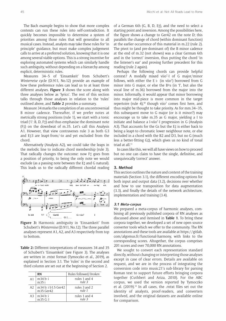
Measures 34–5 of ‘Einsamkeit’ from Schubert’s Winterreise cycle (D.911, No.12) provide an example of how these preference rules can lead us to at least three different analyses. Figure 3 shows the score along with three analyses below as ‘lyrics’. The rest of this section talks through those analyses in relation to the ‘rules’ outlined above, and Table 2 provides a summary.

Measure 34 marks the completion of an uncontroversial B minor cadence. Thereafter, if we prefer notes at metrically strong positions (rule 1), we start with a tonic triad (‘i’: B, D, F) and thus emphasise the dominant note (F) on the downbeat of m.35. Let’s call this Analysis A1. However, that view contravenes rule 3 as both G3 and E3 are leapt-from/-to and yet excluded from the chord.

Alternatively (Analysis A2), we could take the leaps in the melodic line to indicate chord membership (rule 3). That radically changes the outcome: now F goes from a position of priority, to being the only note we would exclude (as a passing note between the E and G natural). This leads us to the radically different chordal reading

of a German 6th (G, B, D, E), and the need to select a starting point and inversion. Among the possibilities here, the figure shows a change to Ger42 on the note D; this parallels the change of chord (within dominant function) at the earlier occurrence of this material in m.22 (rule 2). The pivot to (and pre-dominant of) the B minor cadence at the end of m.32 (not shown) was a clear German 6th and in the ‘correct’ inversion, thus putting the chord ‘in the listener’s ear’ and proving further precedent for this reading (rule 2 again).

Perhaps the following chords can provide helpful context? A modally mixed viio7-I of G major/minor follows, with either the E♭ (in viio7) borrowed from G minor into G major, or else the B♮s (in ‘I’, but also the vocal line of m.36) borrowed from the major into the minor. Informally, it would appear that minor borrowing into major mid-piece is more common in the target repertoire (rule 4),10 though viio7 comes first here, and thus might be thought to take priority. As for mm.34–35, this subsequent move to G major (or is it minor?) may encourage us to take m.35 as G major, yielding a I to initiate and balance a I-viio7-I progression in G (Analysis A3). That accounts for the Gs but the E is either back to being a leapt-to chromatic lower neighbour note, or else included in a chord with the B2 and D3, but no G (much less a better-fitting G), which gives us no kind of tonal triad at all.11

In cases like this, we will all have views on how to proceed but no one can claim to have the single, definitive, and unequivocally ‘correct’ answer.

3. MethodThis section outlines the nature and content of the training materials (Section 3.1), the different encoding options for both input and output data (3.2), decisions over whether and how to use transposition for data augmentation (3.3), and finally the details of the network architecture, implementation and training (3.4).

3.1 Meta-corpusWe prepared a meta-corpus of harmonic analyses, com-bining all previously published corpora of RN analyses as discussed above and itemised in Table 1. To bring these corpora together, we developed a set of new open source converter tools which we offer to the community. The RN annotations and these tools are available at https://gitlab.com/algomus.fr/functional-harmony, with links to the corresponding scores. Altogether, the corpus comprises 201 scores and over 70,000 RN annotations.

We sought to convert each representation standard directly, without changing or interpreting those analyses except in case of clear errors. Details are available on request, and we are in the process of integrating the conversion code into music21’s sub-library for parsing Roman text to support future efforts bringing corpora together (Cuthbert and Ariza, 2010). For the ABC corpus, we used the version reported by Tymoczko et al. (2019).12 In all cases, the .rntxt files set out the identity of analysts, proof-readers, and converters involved, and the original datasets are available online for comparison.

Table 2: Different interpretations of measures 34 and 35 of Schubert’s ‘Einsamkeit’ (see Figure 3). The analyses are written in .rntxt format (Tymoczko et al., 2019), as explained in Section 3.1. The ‘rules’ in the second and third column are set out at the beginning of Section 2.

RN Rules followed/broken

A1 m34 b: i rules 1 and 4m35 i rule 3

A2 m34 b: i b1.5 Ger42 rules 3 and 2m35 Ger42 rule 1

A3 m34 b: i rules 1 and 4m35 G: I rule 3

Figure 3: Harmonic ambiguity in ‘Einsamkeit’ from Schubert’s Winterreise (D.911, No.12). The three parallel analyses represent A1, A2, and A3 respectively from top to bottom.

Micchi et al: Not All Roads Lead to Rome 46

Different Annotators. Among these datasets, ‘TAVERN’ is the only one to include more than one alternative reading of the same piece by different annotators, a feature that is useful for communicating to the algorithm that there can be multiple valid readings of the same passage. For example, some annotators may prefer to define fewer chord changes in order to emphasise longer-range structure of the piece (excluding many notes as non-chord tones); others may include more of those notes, leading to a narrower focus on momentary changes.

In this study, for the sake of simplicity, we elected to treat each of these analyses independently. It is clearly not quite right to treat multiple analyses of the same music as equivalent to analyses of separate pieces, and doing so will introduce some bias in the model; however, we consider this a small detraction relative to the gain in variance afforded by the alternative readings.

Additionally, while the other datasets consistently offer one analysis per piece, by drawing them together, we have integrated a broad range of analytical perspectives. Again we consider that diversity an asset above and beyond the simple gain in scale, though we are not in a position to make any claims towards a ‘balance’ of approaches represented, and certainly not to ‘representativeness’. For instance, each of the original datasets focuses on a different style, and so there is a non-separable correlation between annotators and musical genres. Future work could explore inter-annotator stylistic variance, in order to get a data-driven sense of the variety of approaches and how best to balance them as the provision of corpora continues to grow.

Data Formats. Whatever the original formats of our data, we have elected here to use three formats which we find collectively offer the best balance between uniformity and suitability to the range of tasks involved. For analysis input, we recommend the human-readable and music21-parseable ‘Roman text’ (.rntxt) format (Tymoczko et al., 2019); for the presentation of results aligned with scores, we offer .json files that can be interpreted and visualised by Dezrann (Giraud et al., 2018); and for machine learning, we prefer a tabular representation based on that originally proposed by Chen and Su (2018).

This last, tabular format encodes RN analyses according to six properties:

1. Start offset: the beginning of the annotation in question as measured from the start of the score in ‘quarter length’ (1 = 1 quarter note);

2. End offset: an equivalent for where the annotation ends (usually coincident with the start of the next entry);

3. Key: tonic, specifying full pitch spelling (so that G ≠ A♭) and mode (uppercase for major; lowercase for minor);

4. Quality: for example, major or minor triad; major, minor, or dominant seventh;

5. (Scale) Degree: from 1 (the tonic) to 7 with the po-tential for accidental modifications (e.g. 4) and/or secondary, ‘tonicised’ degrees (5/5); and

6. Inversion: counting from 0 (root position: bass note = chord root) to a maximum of 3 (thus supporting all inversions of seventh chords, but no ninths).

Table 3 sets out the beginning of the Bach prelude from Figure 1 with the Roman text and tabular representations aligned for comparison.

3.2 Encoding Input and OutputsIdentifying best practice in the encoding of musical information for machine learning is an open problem (Huang et al., 2018; Briot et al., 2020). One consideration we know to be highly relevant in determining the best approach is the size of the dataset. While our dataset is larger than previous efforts, it is still small by the standards and requirements of machine learning. This redoubles the significance of the representation format: we want to include all relevant information, but the more we compress that information, the fewer parameters the system has to learn, and the more one can achieve with a smaller dataset. This section addresses the three primary aspects of data encoding for our purposes: time, pitch, and RN representation.

Time. The literature proposes two main approaches to time encoding. The first (Oore et al., 2018) represents the score as a series of three possible event types: note on, note off, and time shift (following MIDI conventions). A time shift event defines the distance between two successive note events. This representation overcomes certain problems particularly common in music generation tasks,13 but it can conceal the music’s metrical structure, which is important in harmonic analysis.

Much better represented in the literature is the alternative ‘frame-based’ encoding method, where each input vector denotes an individual time frame. Most studies on symbolic music opt for some factor-of-two multiple for the smallest slice (1/8th, 1/16th, or 1/32nd notes) and accept the errors that this will entail for shorter values and for all triplets (which are quantised to binary positions).

We follow this latter practice for equal-duration, binary division frames. In our case, we use a 32nd note for input encoding (notes) and 8th note for the output (chords), as the harmonic rhythm is almost always (much) slower

Table 3: The RN and tabular representations used corre-sponding to the Bach extract in Figure 1. The first col-umn sets out RNs in Tymoczko et al. (2019)‘s ‘Roman text’ format, and the remaining columns unpack that information according to our adaptation of Chen and Su (2018)‘s tabular standard.

RNTXT Start End Key Degree Quality Inv.

m1 C: I 0.0 4.0 C 1 M 0m2 ii42 4.0 8.0 C 2 m7 3m3 V65 8.0 12.0 C 5 D7 1m4 I 12.0 16.0 C 1 M 0m5 vi6 16.0 20.0 C 6 m 1m6 G: V42 20.0 24.0 G 5 D7 3m7 I6 24.0 28.0 G 1 M 1m8 IV42 28.0 32.0 G 4 M7 3m9 ii7 32.0 36.0 G 2 m7 0m10 V7 36.0 40.0 G 5 D7 0m11 I 40.0 44.0 G 1 M 0

Micchi et al: Not All Roads Lead to Rome47

than the surface rhythm. Finally, we divide all scores in segments of equal quarter-note duration and pad with zeroes to the right when needed.

Pitch. The options for pitch encoding may be set out in two dimensions. The first accounts for pitch spelling. Here we must choose between using pitch class representations (12 per octave, and no difference between the enharmonic equivalent pairs like G and A♭), or maintaining the full pitch spelling (with 21 possibilities per octave for single sharps/flats and 35 for double).14

The other dimension concerns registral information. Keeping octave information leads to richer data, but excluding it would be more compact. We propose a third, ‘compromise’ option reflecting the special role of the bass in tonal harmony in defining both chordal inversion and other important matters for harmonic progression. In this case, music is encoded with two vectors per frame: one with the lowest note and another with the total pitch content. The fact that the lowest note may not be indicative of the bass is one of the many tasks that the system would need to learn. Table 4 sets out these options with their relative size for the case of a 7-octave space and chromatic spellings of up to double sharps/flats.

Regardless of the pitch space chosen, we define a Boolean matrix with time frames on one axis and pitches on the other: The value is 1 if the pitch is present in that frame, and 0 otherwise. In this encoding, multiple pitches may be activated in the same time frame where they sound simultaneously in the source (as in chords, for example). This data representation reduces to the familiar piano roll notation when using CPf for the pitch space.

One potential shortcoming of such a frame-based encoding is that it fails to distinguish between repeated and held notes. Hadjeres et al. (2017) and Liang et al. (2017) include special symbols to disambiguate this on voice-separated music. When the number of voices is not fixed, one symbol per note is required, doubling the size of the input vector. We decided not to encode that information partly due to the loss of compactness, but also because we do not expect distinguishing tied from repeated notes to be especially important for harmonic analysis.

RN Output Labels. Continuing to follow Chen and Su (2018) we output the harmonic analysis with six labels: Key, Degree 1, Degree 2, Quality, Inversion, and Root. The two labels for scale degrees handle cases of tonicisations in the format ‘Degree 2/Degree 1’. The labels for keys and chord

roots depend on the choice of the input representations. For all CP cases there are 12 possible chord roots and 24 keys (12 major and 12 minor). When the input is in a PS encoding, the number of possibilities increases: there are 35 roots and thus 70 keys for the double sharp/flat condition.15

There is some redundancy built into this system as it is possible to derive the root unambiguously from other features. However, learning redundant variables can be helpful to the algorithm’s success. The division of each RN label into six independently-computed sub-labels reduces the complexity of the task, since the total number of possible outputs for our best-performing representation is Σici = 123 ≪ ∏ici ≈ 22⋅106, where ci is the number of output classes for each separate target label. It also improves the interpretability of the results, allowing one to focus on each aspect separately.

This comes at the cost of a potential for self-contradictory outputs in which the six sub-labels have different ideas about the chord. In practice, we find that this is only rarely a problem, arising in the particular case of the ‘no chord’ label used by the ABC dataset (only) for passages with rests and/or single line melodies. Given the inconsistency in the source data, we do not include a provision for the ‘no chord’ case. Instead, we fill any such gap with a continuation of the foregoing chord, except in the case of beginnings, for which we start the first chord early.

3.3 Data Augmentation by TranspositionIn practice, keys are not used equally. It is common in both analysis and generation tasks to augment the dataset by transposing it to multiple keys (Huang et al., 2018; Chen and Su, 2019). While a single piece in two transpositions should not be considered equivalent to two distinct pieces (for reasons somewhat analogous to the status of multiple analyses of the same piece discussed above), transposition does stand to augment considerably the overall size of the dataset.

While working within the ‘CP’ encoding space (as is the case for all work based on MIDI), there are only 12 distinct transpositions: one for each distinct pitch class.

When including pitch spelling, transposition moves not through a circle, but a spiral, potentially infinitely. Clearly, some constraint is required to limit this pitch space. We define two such constraints, both based on the ‘spiral of fifths’ where pitch objects (usually keys) are set out according to their relative flat-/sharp-ness.

Our first constraint limits the pitches to double flats/sharps from F♭♭ to B. To enforce this constraint, we need to retrieve the ‘chromatic ambitus’ of each piece, delimited by the ‘flattest’ and ‘sharpest’ pitches used. For instance, Schubert’s ‘Einsamkeit’ (Figure 3) ranges from E♭ to E, meaning that it can be transposed by 12 further steps in the flat direction and 8 steps sharpwards while still remaining within the set limit of double sharps and flats.

Our second constraint limits the keys to a narrower range from C♭ to C majors and their relative minors (A♭ to A) such that the diatonic pitches are limited to single flats/sharps. We do this to reduce the computational load

Table 4: Total dimension of input vector for each pitch encoding option (limited to 7 octaves and double sharps/flats).

Chromatic pitch, full (CPf)7 × 12 = 84

Pitch spelling, full (PSf)7 × 35 = 245

CP class + bass (CPb)12 + 12 = 24

PS class + bass (PSb)35 + 35 = 70

CP class (CPc)12

PS class (PSc)35

Micchi et al: Not All Roads Lead to Rome 48

without losing actual information, as real pieces very rarely go outside these key boundaries. For this constraint, we need to look at the chord labels. In the Schubert example, by almost any reading, the sharp-most key used is B minor (5 steps away from the limit of A on the spiral of fifths), and the flatmost is C minor (4 steps away from A♭).

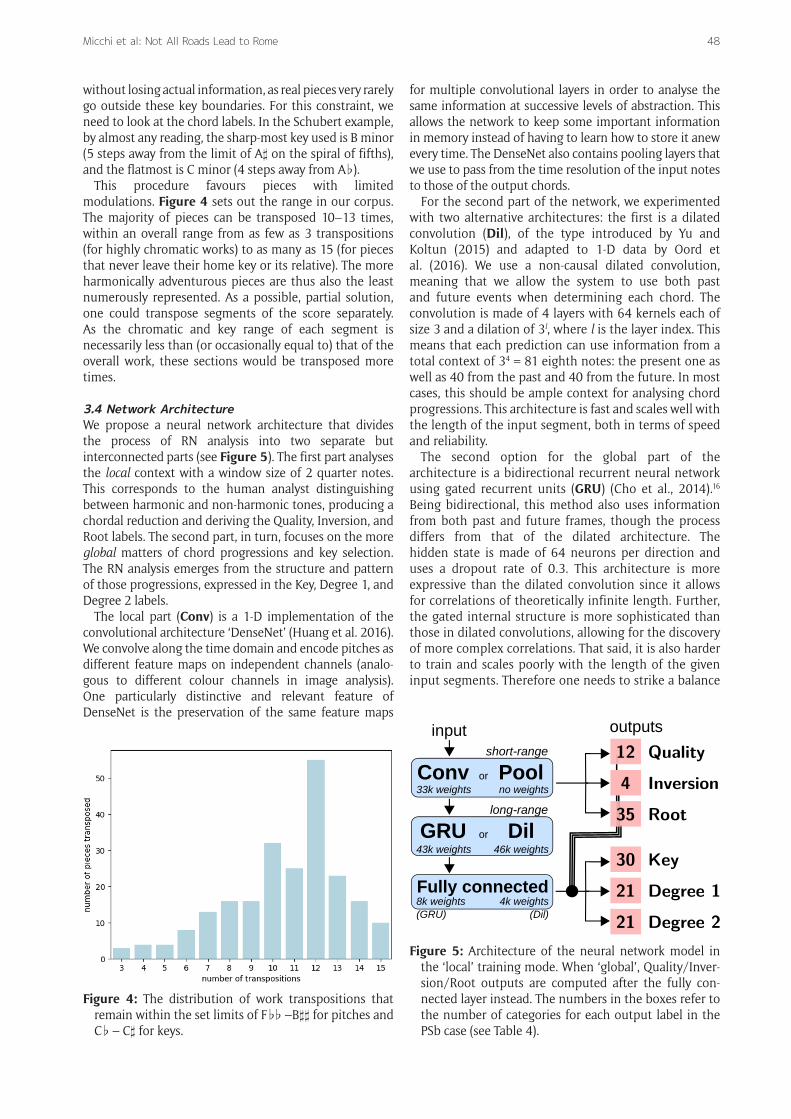
This procedure favours pieces with limited modulations. Figure 4 sets out the range in our corpus. The majority of pieces can be transposed 10–13 times, within an overall range from as few as 3 transpositions (for highly chromatic works) to as many as 15 (for pieces that never leave their home key or its relative). The more harmonically adventurous pieces are thus also the least numerously represented. As a possible, partial solution, one could transpose segments of the score separately. As the chromatic and key range of each segment is necessarily less than (or occasionally equal to) that of the overall work, these sections would be transposed more times.

3.4 Network ArchitectureWe propose a neural network architecture that divides the process of RN analysis into two separate but interconnected parts (see Figure 5). The first part analyses the local context with a window size of 2 quarter notes. This corresponds to the human analyst distinguishing between harmonic and non-harmonic tones, producing a chordal reduction and deriving the Quality, Inversion, and Root labels. The second part, in turn, focuses on the more global matters of chord progressions and key selection. The RN analysis emerges from the structure and pattern of those progressions, expressed in the Key, Degree 1, and Degree 2 labels.

The local part (Conv) is a 1-D implementation of the convolutional architecture ‘DenseNet’ (Huang et al. 2016). We convolve along the time domain and encode pitches as different feature maps on independent channels (analo-gous to different colour channels in image analysis). One particularly distinctive and relevant feature of DenseNet is the preservation of the same feature maps

for multiple convolutional layers in order to analyse the same information at successive levels of abstraction. This allows the network to keep some important information in memory instead of having to learn how to store it anew every time. The DenseNet also contains pooling layers that we use to pass from the time resolution of the input notes to those of the output chords.

For the second part of the network, we experimented with two alternative architectures: the first is a dilated convolution (Dil), of the type introduced by Yu and Koltun (2015) and adapted to 1-D data by Oord et al. (2016). We use a non-causal dilated convolution, meaning that we allow the system to use both past and future events when determining each chord. The convolution is made of 4 layers with 64 kernels each of size 3 and a dilation of 3l, where l is the layer index. This means that each prediction can use information from a total context of 34 = 81 eighth notes: the present one as well as 40 from the past and 40 from the future. In most cases, this should be ample context for analysing chord progressions. This architecture is fast and scales well with the length of the input segment, both in terms of speed and reliability.

The second option for the global part of the architecture is a bidirectional recurrent neural network using gated recurrent units (GRU) (Cho et al., 2014).16 Being bidirec tional, this method also uses information from both past and future frames, though the process differs from that of the dilated architecture. The hidden state is made of 64 neurons per direction and uses a dropout rate of 0.3. This architecture is more expressive than the dilated convolution since it allows for correlations of theoretically infinite length. Further, the gated internal structure is more sophisticated than those in dilated convolutions, allowing for the discovery of more complex correlations. That said, it is also harder to train and scales poorly with the length of the given input segments. Therefore one needs to strike a balance

Figure 5: Architecture of the neural network model in the ‘local’ training mode. When ‘global’, Quality/Inver-sion/Root outputs are computed after the fully con-nected layer instead. The numbers in the boxes refer to the number of categories for each output label in the PSb case (see Table 4).

short-range

Conv Poolor33k weights no weights

43k weights 46k weights

8k weights 4k weights(GRU) (Dil)

Fully connected

Quality12

Root35

Key30

Degree 121

Degree 221

Inversion4

input outputs

long-range

GRU Dilor

Figure 4: The distribution of work transpositions that remain within the set limits of F♭♭–B for pitches and C♭– C for keys.

Micchi et al: Not All Roads Lead to Rome49

in terms of segment length: segments must be long enough to take advantage of the recurrent nature of the network, but short enough to make training feasible. We elected to divide the scores in non-overlapping segments of 80 quarter notes’ duration.

With either architecture, the second part ends with a fully connected layer of 64 neurons. Each label is predicted by a fully connected layer with softmax activation, whose size is determined by the number of classes for the label at hand. The network is trained end-to-end to ensure strong connection between the local and global tasks. The loss function used is the standard categorical cross-entropy loss. This is computed on each of the six target labels separately before the results are added, with an equal weighting.

As a baseline for comparison of these two approaches, we also trained a standard GRU model without local context analysis. We refer to this as PoolGRU as it is preceded by pooling layers to reduce the resolution on the time axis.

3.5 Network TrainingWe randomly allocated 90% of the available scores to the training set, reserving the remaining 10% for validation. Importantly, we implemented this proportion not only for the corpus overall, but for each of the corpora individually. For the special case of TAVERN, those works assigned to the training set included the score and both of the corresponding analyses; pieces in the validation by contrast included only one of the analyses (randomly selected). In order to provide direct comparison with Chen and Su (2018, 2019), we also calculated results using only their dataset, divided in the same way.

We trained in two ways. In the first (global) approach, all six labels are predicted at the end of the second part (Dil or GRU). In the second (local) method, the Quality, Inversion, and Root labels are determined at the end of the first, local part of the network and used to determine the key and degree. As discussed, we did not enforce consistency between labels. Given the lack of local context, PoolGRU can only be trained in global mode.

The network was encoded in Python v3.7 using Tensorflow v1.14. The code is available at https://gitlab.com/algomus.

fr/functional-harmony and was initially forked from Chen and Su (2018), but all dataset conversions, encodings, and models are original work. Our best model has about 94,000 trainable weights in total: 33,000 for the local part, 43,000 for the global, and the remaining 18,000 for the fully connected layers. Depending on the model, the total training time ranges from 20 minutes to 3 hours, when run on a CPU-only high-performance-computing server.

4. Results4.1 Overall MetricsThe results for our best model (ConvGRU, PSb, global learning) are summarized and compared with Chen and Su (2018, 2019) in Table 5. The first row sets out the results obtained by our best model using the new meta-corpus, while the second row reports on results limited to Chen and Su’s own dataset for direct comparison. At a glance, one can see that our proposal achieves a small but significant improvement over the previous state-of-the-art while also taking full pitch spelling into account.

Our emphasis here is on comparing the different encodings and the architectures, and on attempting to identify edge cases. To that effect, we have trained on all possible combinations of the six pitch encodings, the two architectures (and the baseline), and the two training types (except for PoolGRU, which is only applicable for global training). Table 6 presents the results averaged over all of the models.

As the table shows, ConvGRU (mixing local analysis and a GRU unit) is the best performing architecture, surpassing the two alternatives, with a particularly significant improvement over PoolGRU. Indeed, a t-test on the significance of the difference for the full task (the column ‘RN’ in Table 6) yielded a p-value < 10–2 against the null hypothesis of ConvGRU and PoolGRU giving the same result.

As for the pitch encoding, including the bass information (CPb/PSb) results in markedly higher performance not only in identifying the correct inversions, but for all of the tasks (again, p-value < 10–2). On the other axis of pitch representation, using full pitch spelling generally leads to slightly higher results overall, but the results are not statistically significant. That said, we must remember

Table 5: Comparison of the percent accuracy between models. The two rows above the internal division report on our best model – ConvGRU with pitch spelling and bass (PSb) and with global training. The first row reports on training with all available data; the second reduces the available data to the smaller corpus used by Chen and Su (2018). Rows below the internal dividing line provide comparison data for the performance of Chen and Su (2018, 2019), as well as a baseline key detection using pitch profiles by Temperley (1999). ‘Degree’ registers as correct only when the predic-tions match the corpus entry for both Degrees 1 and 2; ‘RN’ is correct only when all four of the previous columns match in that way.

Key Degree Quality Inversion RN

ConvGRU + PSb + global (all data) 82.9 68.3 76.6 72.0 42.8ConvGRU + PSb + global 80.6 66.5 76.3 68.1 39.1

Chen and Su (2019) 78.4 65.1 74.6 62.1Chen and Su (2018) 66.7 51.8 60.6 59.1 25.7Local model after Temperley (1999) 67.0

Micchi et al: Not All Roads Lead to Rome 50

that analyses without pitch spelling cannot distinguish between enharmonically equivalent keys like G and A♭. As such, the inclusion of spelling means introducing more keys and chord roots and thus amounts to a more difficult task where proportionately fewer answers will be correct. As pitch spelling yields performances that are not worse while performing a harder, more musically relevant task, we conclude that the spelling representation is preferable where the data is available.

Comparing local and global training yields a much more ambiguous result that invites further study. The difference in the total result is statistically not significant. However, when one looks at specific (local) labels such as the quality, one finds that the differences in the intermediate steps taken by the two architectures are significant (with a p-value against the null hypothesis smaller than 10–6).

4.2 A Closer Look at the MusicAs this discussion of overall accuracy metrics would seem to indicate, there is more to the task of evaluating the results of an RN analysis. As such, we continue here to take a closer look at the ‘errors’ made by the models. These ‘errors’ – or, more properly, divergences between the input corpus and prediction – appear to centre on three main types:

1. Segmentation errors: differences in the timing of chord changes (see Bach prelude, Table 7). This appears to be the most common discrepancy. More specifically, we notice that the predictions tend to change more frequently than the human analy-ses, particularly in more complex passages. This is presumably on the basis of an attempt to divide the music into small enough segments to allow a cleaner reading of the chord in those small spans. Strategies such as the segmenter layer proposed by Chen and Su (2019) may help.

2. Mislabeling of rare chords: the system is highly reluctant to identify secondary/tonicised chords or chromatic chords like the augmented sixths, presumably because they are relatively rare in the corpus.

3. Alternative readings: moments where the system opts for a reading that is different from that of the validation corpus, but which is nonetheless a perfectly acceptable alternative. Corpora with multiple readings of the same music would be especially helpful here because they offer the system not a single ‘correct’ answer, but a list of viable options.

Once again, the extract from Schubert’s ‘Einsamkeit’ (discussed in Section 2 and shown in Figure 3) offers a neat example of all three issues. Our reference analysis corresponds broadly to analysis A2. Regarding issue 1, the prediction for measures 34 and 35 is made of four different chord labels, while in the reference dataset there are only two. This is strictly connected with issue 2, as the ‘mis’-labeled chord is a German sixth, unidentified by our system. Lastly, ‘the different but acceptable’ reading is pertinent in the case of measures 36 and following, which the dataset analyses in terms of G minor, the system views in G major, and is in fact an ambiguous mixture of the two (as discussed in Section 2).

Finally, we found some cases we consider unacceptable readings, where the most compelling musical reading diverges from the statistically normative case. For example, in Beethoven’s sixth sonata (op.10 no.2, Figure 6), the exposition includes a theme in C major which from measure 41 is repeated in the parallel key of C minor. Perhaps because this lasts for only four measures, the system is reluctant to identify a full modulation, preferring instead to remain in C major.

Table 6: Results obtained by averaging the accuracy of several models on four different axes: architecture, input regis-tral information, input spelling, and global/local training. Column labels are the same as for Table 5, and the first row likewise relates once again to the best performing model. Each sub-table thereafter shows the average performance of several models. For example, the ConvGRU row shows the average of 12 models with the same architecture but using different input representations and registral information. The values in the first row of each sub-table repre-sent the percentage accuracy of the corresponding averaged models as a reference; each line thereafter shows the +/– difference in accuracy from the reference. There are only 6 PoolGRU models, as they can be trained only globally (not locally).

Key Degree Quality Inversion RN

ConvGRU + PSb + global 82.9 68.3 76.6 72.0 42.8

ConvGRU 12 81.9 67.4 74.6 67.9 37.8ConvDil 12 –2.4 –1.8 –0.8 –0.5 –1.7PoolGRU 6 –2.3 –3.0 –1.6 –1.8 –4.1

bass 10 80.8 66.6 74.3 70.1 39.2full 10 –0.7 –0.9 –0.6 –3.5 –3.7class 10 –0.1 –0.7 –0.1 –4.7 –4.7

spelling 15 80.6 66.2 74.1 67.6 36.5chromatic 15 –0.3 –0.3 –0.2 –0.5 –0.4

global 15 80.6 66.8 75.4 66.7 36.9local 15 +0.3 –0.7 –2.4 +2.0 +0.2

Micchi et al: Not All Roads Lead to Rome51

5. Future Work5.1 ImprovementsA simple right/wrong accuracy metric is not the best way to measure the performance of an RN analysis algorithm, as several different readings are often equally viable. Even taking this into account, the 43% total accuracy that we report is still far from ideal. In this concluding section, we propose some ideas for improving these results.

As mentioned above, this field would benefit greatly from larger datasets, covering both a wider repertoire and multiple, alternative readings of the same works.

It would also be useful to explore wider encoding options, and not just for pitch and time: for the repertoires discussed here, metrical position, dynamics, texture, and other score indications are also strongly attested to have a bearing on harmonic analysis. Including those parameters may improve performance, though informal testing of metrical strength did not yield significant gains, and the quality of machine-readable score encoding often prohibits a serious analysis of parameters like dynamics.

In the time domain, comparisons could include assess-ing the relative performance of the ‘frame-based’ approach with the alternative ‘variable length’ convention (Oore et al., 2018). This latter allows representation of arbitrarily short and long time spans and would save on training time (by virtue of it reducing the total number of entries). It may also better reflect the human experience of music, which does not proceed in granular units, but centres on the information density of events and changes.

In the pitch domain, it would be interesting to define a space for the relative proximity of pitches and to add a second convolutional dimension on that space. This may lead to an improvement on the current model of using independent channels. Most simply, this could involve

implementing the ‘line’ or ‘spiral’ of fifths (mentioned above in connection with transposition), and proposals for more complex spaces to explore abound.17

Relatedly, the evaluation of output could be improved, perhaps through the definition of relative distance in functional terms. This would entail a distance metric between chords to write a more ‘musically relevant’ loss function which considers chords of the same function (such as ii7 and IV) to be closer to one another than to those of a different function (V7). This could also prove helpful for cases with multiple annotators, providing a metric for the relative divergence between those readings.

Additionally, while interpreting the results of a machine learning method is always difficult, this would help to advance our understanding both of the processes in operation here, and by extension, of harmony itself. One possible way of accomplishing this is to follow the activation of the neurons in a set of simple example cases.

Finally, one could also explore a combination of learned and/or deterministic post-processing to enforce the kind of consistency between labels discussed above. It may be that approaches combining machine learning, deterministic algorithms, and a human-in-the-loop achieve results surpassing those accomplished by each of these methods separately.

5.2 ApplicationsWe view the whole endeavour of (semi-)automated harmonic analysis as a means to the end of understanding harmony better. As such, one goal is to produce harmonic analyses at a sufficiently high quality level that they constitute a reliably usable dataset – and object of study – in themselves. This would enable us to scale up questions of how harmonies ‘tend to’ be used, enabling the field of corpus analysis to realise its potential.

We consider it important that the models we proposed can be adapted to other kinds of harmonic analyses. As discussed above, harmonies in lead sheets have a different ontological status from RNs, and the repertoires represented are stylistically divergent, but the technical problem is comparable and often contained within the framework of the RN analysis.

Table 7: A comparison between the corpus analysis (left, reproducing Table 3) and our system’s output (right). Dis-crepancies between the input and output analyses are highlighted in italics.

RN Corpus OutputStart End Key Degree Quality Inv. Start End Key Degree Quality Inv.

m1 C: I 0.0 4.0 C 1 M 0 0.0 4.0 C 1 M 0m2 ii42 4.0 8.0 C 2 m7 3 4.0 4.5 C 2 m7 0

4.5 7.0 C 2 m7 17.0 7.5 C 2 D7 07.5 8.0 C 5 D7 0

m3 V65 8.0 12.0 C 5 D7 1 8.0 8.5 C 5 D7 18.5 9.5 C 5 M 19.5 10.0 C 5 D7 110.0 11.0 C 5 M 111.0 12.0 C 5 D7 1

m4 I 12.0 16.0 C 1 M 0 12.0 16.0 C 1 M 0m5 vi6 16.0 20.0 C 6 m 1 16.0 16.5 C 1 m 0

16.5 17.0 C 6 m 017.0 20.0 C 6 m 1

Figure 6: Beethoven’s piano sonata no.6, m.40–43.

Micchi et al: Not All Roads Lead to Rome 52

Finally, we welcome further work on the public-facing side of such research. To this end, we are developing a web application which will allow the wider musical community to experiment with the harmonic analyses generated by our model on any score they might provide. We hope that this will enable and encourage the community to share ideas about harmonic analysis in general, and on how to improve this model in particular.

Notes 1 See for instance the contents pages of recent textbooks

like Clendinning and Marvin (2016); Laitz (2016). 2 http://jazzparser.granroth-wilding.co.uk/ParserPaper.

html. 3 http://rockcorpus.midside.com. 4 https://zenodo.org/record/1476555#.XebL6C3

Myu4. 5 h t tp :// jazzomat .h fm-weimar.de/dbformat/

dbcontent.html. 6 https://zenodo.org/record/1290737$\sharp$ .

W6vIKxNKixM. 7 http://ddmal.music.mcgill.ca/research/billboard. 8 https://csml.som.ohio-state.edu/home/index.php/

iRb_Jazz_Corpus. 9 http://www.isophonics.net/datasets. 10 ‘Mid-piece’ is significant because of the relatively

common practice of ending minor key pieces with a major triad (with the so-called ‘Picardie’ third).

11 The chord could be re-spelled enharmonically as B diminished, though even that would hardly help the wider reading.

12 See https://github.com/DCMLab/ABC/issues for ongoing discussion over issues with the original corpus. Both Tymoczko et al. and Neuwirth et al. have plans to release a corrected and updated version of this corpus; that would effectively provide a second multiple-annotator dataset with which to study inter-annotator variance.

13 These include the disproportionate difficulty in predic-ting long notes that arises from having to make the correct prediction anew for each frame.

14 Systems using MIDI are necessarily limited to the former; the latter is only available to richer input formats like **kern, MusicXML, and MEI.

15 However, not all those keys can actually be used because some diatonic pitches would have triple flats or sharps. We will discuss more about what keys we actually use in the next section.

16 We prefer GRUs over LSTM cells due to their greater compactness.

17 For historical examples, see (Heinichen (1711); Euler (1739); Oettingen (1866); Schoenberg (1948); and for more models, see (Lewin (1987); Cross (1997); Cohn (1999); Tymoczko (2011); Cohn (2012).

AcknowledgementsWe gratefully acknowledge support from the CPER MAuVE, ERDF, Hauts-de-France (Gianluca Micchi), and Cornell University’s Active Learning Initiative and the Université de Lille’s ‘Invited Researcher Residency’ scheme (Mark Gotham). We also wish to thank the Mésocentre de

Lille for their computing resources, and especially Cyrille Toulet for his assistance.

Competing InterestsThe authors have no competing interests to declare.

ReferencesBriot, J.-P., Hadjeres, G., & Pachet, F.-D. (2020). Deep

Learning Techniques for Music Generation. Compu-tational Synthesis and Creative Systems. Springer. DOI: https://doi.org/10.1007/978-3-319-70163-9

Chen, T.-P., & Su, L. (2018). Functional harmony recognition of symbolic music data with multi-task recurrent neural networks. In International Society for Music Information Retrieval Conference (ISMIR 2018).

Chen, T.-P., & Su, L. (2019). Harmony Transformer: Incorporating chord segmentation into harmony recognition. In International Society for Music Information Retrieval Conference (ISMIR 2019).

Cho, K., van Merrienboer, B., Gulcehre, C., Bahdanau, D., Bougares, F., Schwenk, H., & Bengio, Y. (2014). Learning phrase representations using RNN encoder-decoder for statistical machine translation. arXiv:1406.1078. DOI: https://doi.org/10.3115/v1/D14-1179

Clendinning, J. P., & Marvin, E. W. (2016). The Musician’s Guide to Theory and Analysis. W.W. Norton, 3rd edition.

Cohn, R. (1999). As wonderful as star clusters: Instru-ments for gazing at tonality in Schubert. 19th-Century Music, 22(3), 213–232. DOI: https://doi.org/10.1525/ncm.1999.22.3.02a00020

Cohn, R. (2012). Audacious Euphony: Chromatic Harmony and the Triad’s Second Nature. Oxford Studies in Music Theory. Oxford University Press, USA.

Cross, I. (1997). Pitch schemata. In I. Deliège & J. Sloboda (Eds.), Perception and Cognition of Music, pages 357–390. Psychology Press, Hove.

Cuthbert, M. S., & Ariza, C. (2010). music21: A toolkit for computer-aided musicology and symbolic music data. In International Society for Music Information Retrieval Conference (ISMIR 2010), pages 637–642.

de Clercq, T., & Temperley, D. (2011). A corpus analysis of rock harmony. Popular Music, 30(1), 47–70. DOI: https://doi.org/10.1017/S026114301000067X

De Haas, W. B., Rohrmeier, M., Veltkamp, R. C., & Wiering, F. (2009). Modeling harmonic similarity using a generative grammar of tonal harmony. In International Society for Music Information Retrieval Conference (ISMIR 2009), pages 549–554.

Devaney, J., Arthur, C., Condit-Schultz, N., & Nisula, K. (2015). Theme and variation encodings with Roman numerals (TAVERN): A new data set for symbolic music analysis. In International Society for Music Information Retrieval Conference (ISMIR 2015).

Duinker, B. (2019). Plateau loops and hybrid tonics in recent pop music. Music Theory Online, 25(4). DOI: https://doi.org/10.30535/mto.25.4.3

Euler, L. (1739). Tentamen Novae Theoriae Musicae ex Certissimis Harmoniae Principiis Dilucide Expositae. Saint Petersburg Academy.

Micchi et al: Not All Roads Lead to Rome53

Giraud, M., Groult, R., & Leguy, E. (2018). Dezrann, a web framework to share music analysis. In International Conference on Technologies for Music Notation and Representation (TENOR 2018), pages 104–110.

Hadjeres, G., Pachet, F., & Nielsen, F. (2017). Deep-Bach: A steerable model for Bach chorales generation. In Proceedings of the 34th International Conference on Machine Learning – Volume 70, ICML’17, page 1362–1371. JMLR.org.

Harasim, D., Rohrmeier, M., & O’Donnell, T. J. (2018). A generalized parsing framework for generative models of harmonic syntax. In International Society for Music Information Retrieval Conference (ISMIR 2018), pages 152–159.

Heinichen, J. D. (1711). Neu erfundene und gründliche Anweisung – zu vollkommener Erlernung des General-Basses. Schiller, Hamburg.

Holtzman, S. R. (1977). A program for key determina-tion. Interface, 6, 29–56. DOI: https://doi.org/10. 1080/09298217708570231

Huang, C.-Z. A., Vaswani, A., Uszkoreit, J., Shazeer, N., Simon, I., Hawthorne, C., Dai, A. M., Hoffman, M. D., Dinculescu, M., & Eck, D. (2018). Music Transformer. arXiv:1809.0428.

Huang, G., Liu, Z., van der Maaten, L., & Weinberger, K. Q. (2016). Densely connected convolutional networks. arXiv:1608.06993. DOI: https://doi.org/10.1109/CVPR. 2017.243

Illescas, P. R., Rizo, D., & Iñesta, J. M. (2007). Harmonic, melodic, and functional automatic analysis. In Interna-tional Computer Music Conference (ICMC 2007), pages 165–168.

Ju, Y., Condit-Schultz, N., Arthur, C., & Fujinaga, I. (2017). Non-chord tone identification using deep neural networks. In International Workshop on Digital Libraries for Musicology (DLfM’17), pages 13–16. DOI: https://doi.org/10.1145/3144749.3144753

Ju, Y., Howes, S., McKay, C., Condit-Schultz, N., Calvo-Zaragoza, J., & Fujinaga, I. (2019). An interactive workflow for generating chord labels for homorhythmic music in symbolic formats. In International Society for Music Information Retrieval Conference (ISMIR 2019).

Krumhansl, C. L., & Kessler, E. J. (1982). Tracing the dynamic changes in perceived tonal organisation in a spatial representation of musical keys. Psychological Review, 89(2), 334–368. DOI: https://doi.org/10.1037/ 0033-295X.89.4.334

Kröger, P., Passos, A., & Sampaio, M. (2008). Rameau: a system for automatic harmonic analysis. In Interna-tional Computer Music Conference (ICMC 2008).

Laitz, S. G. (2016). The Complete Musician: An Integrated Approach to Theory, Analysis, and Listening. Oxford University Press, 4th edition.

Lerdahl, F., & Jackendoff, R. (1983). A Generative Theory of Tonal Music. MIT Press.

Lewin, D. (1987). Generalized Musical Intervals and Transformations. Yale University Press.

Liang, F. T., Gotham, M., Johnson, M., & Shotton, J. (2017). Automatic stylistic composition of Bach

chorales with deep LSTM. In International Society for Music Information Retrieval Conference (ISMIR 2017), pages 449–456.

Madsen, S. T., & Widmer, G. (2007). Key-finding with interval profiles. In International Computer Music Conference (ICMC 2007).

McFee, B., & Bello, J. P. (2017). Structured training for large-vocabulary chord recognition. In International Society for Music Information Retrieval Conference (ISMIR 2017).

Nápoles López, N., Arthur, C., & Fujinaga, I. (2019). Key-finding based on a hidden Markov model and key profiles. In International Workshop on Digital Libraries for Musicology (DLfM’19). DOI: https://doi.org/10.1145/3358664.3358675

Neuwirth, M., Harasim, D., Moss, F. C., & Rohrmeier, M. (2018). The annotated Beethoven corpus (ABC): A dataset of harmonic analyses of all Beethoven string quartets. Frontiers in Digital Humanities, 5. DOI: https://doi.org/10.3389/fdigh.2018.00016

Oettingen, A. (1866). Harmoniesystem in dualer Entwicklung. Leipzig.

Oord, A. V. D., Dieleman, S., Zen, H., Simonyan, K., Vinyals, O., Graves, A., Kalchbrenner, N., Senior, A., & Kavukcuoglu, K. (2016). WaveNet: A generative model for raw audio. arXiv:1609.03499.

Oore, S., Simon, I., Dieleman, S., Eck, D., & Simonyan, K. (2018). This time with feeling: Learning expressive musical performance. Neural Computing and Applications. DOI: https://doi.org/10.1007/s00521- 018-3758-9

Paiement, J.-F., Eck, D., & Bengio, S. (2005). A probabilistic model for chord progressions. In International Conference on Music Information Retrieval (ISMIR 2005).

Pardo, B., & Birmingham, W. P. (2002). Algorithms for chordal analysis. Computer Music Journal, 26(2), 27–49. DOI: https://doi.org/10.1162/014892602760 137167

Robine, M., Rocher, T., & Hanna, P. (2008). Improve-ments of key-finding methods. In International Computer Music Conference (ICMC 2008).

Rocher, T., Robine, M., Hanna, P., & Strandh, R. (2009). Dynamic chord analysis for symbolic music. In International Computer Music Conference (ICMC 2009).

Rohrmeier, M. (2011). Towards a generative syntax of tonal harmony. Journal of Mathematics and Music, 5(1), 35–53. DOI: https://doi.org/10.1080/17459737.2011.573676

Sapp, C. S. (2005). Visual hierarchical key analysis. Computers in Entertainment, 3(4), 3. DOI: https://doi.org/10.1145/1095534.1095544

Schenker, H. (1935). Der freie Satz. Universal Edition.Schoenberg, A. (1954 – op.posth, completed 1948).

Structural Functions of Harmony. Williams and Norgate, London.

Steedman, M., & Longuet-Higgins, H. C. (1971). On interpreting Bach. Machine Intelligence, 6.

Temperley, D. (1997). An algorithm for harmonic analysis. Music Perception: An Interdisciplinary Journal, 15(1), 31–68. DOI: https://doi.org/10.2307/40285738

Micchi et al: Not All Roads Lead to Rome 54

Temperley, D. (1999). What’s key for key? The Krumhansl-Schmuckler key-finding algorithm reconsidered. Music Perception, 17(1). DOI: https://doi.org/10.2307/40 285812

Tymoczko, D. (2011). A Geometry of Music: Harmony and Counterpoint in the Extended Common Practice. Oxford University Press.

Tymoczko, D., Gotham, M., Cuthbert, M. S., & Ariza, C. (2019). The Romantext Format: A flexible and standard method for representing Roman numeral analyses. In International Society for Music Information Retrieval Conference (ISMIR 2019).

Yu, F., & Koltun, V. (2015). Multi-scale context aggrega-tion by dilated convolutions. arXiv:1511.07122.

How to cite this article: Micchi, G., Gotham, M., & Giraud, M. (2020). Not All Roads Lead to Rome: Pitch Representation and Model Architecture for Automatic Harmonic Analysis. Transactions of the International Society for Music Information Retrieval, 3(1), pp. 42–54. DOI: https://doi.org/10.5334/tismir.45

Submitted: 04 December 2019 Accepted: 23 March 2020 Published: 12 May 2020

Copyright: © 2020 The Author(s). This is an open-access article distributed under the terms of the Creative Commons Attribution 4.0 International License (CC-BY 4.0), which permits unrestricted use, distribution, and reproduction in any medium, provided the original author and source are credited. See http://creativecommons.org/licenses/by/4.0/.

Transactions of the International Society for Music Information Retrieval is a peer-reviewed open access journal published by Ubiquity Press. OPEN ACCESS