Embed Size (px)
Citation preview

Status and Trend of Marbled Murrelet Populations and Nesting Habitat
United States Department of Agriculture
Forest Service
Pacific NorthwestResearch Station
General Technical ReportPNW-GTR-933
NORTHWEST FOREST PLAN
The FirsT 20 Years (1994–2013)
Updated January 2018
In accordance with Federal civil rights law and U.S. Department of Agriculture (USDA) civil rights regulations and policies, the USDA, its Agencies, offices, and employees, and institutions participating in or administering USDA programs are prohibited from discriminating based on race, color, national origin, religion, sex, gender identity (including gender expression), sexual orientation, disability, age, marital status, family/parental status, income derived from a public assistance program, political beliefs, or reprisal or retaliation for prior civil rights activity, in any program or activity conducted or funded by USDA (not all bases apply to all programs). Remedies and complaint filing deadlines vary by program or incident.
Persons with disabilities who require alternative means of communication for program information (e.g., Braille, large print, audiotape, American Sign Language, etc.) should contact the responsible Agency or USDA’s TARGET Center at (202) 720-2600 (voice and TTY) or contact USDA through the Federal Relay Service at (800) 877-8339. Additionally, program information may be made available in languages other than English.
To file a program discrimination complaint, complete the USDA Program Discrimination Complaint Form, AD-3027, found online at http://www.ascr.usda.gov/complaint_filing_cust.html and at any USDA office or write a letter addressed to USDA and provide in the letter all of the information requested in the form. To request a copy of the complaint form, call (866) 632-9992. Submit your completed form or letter to USDA by: (1) mail: U.S. Department of Agriculture, Office of the Assistant Secretary for Civil Rights, 1400 Independence Avenue, SW, Washington, D.C. 20250-9410; (2) fax: (202) 690-7442; or (3) email: [email protected].
USDA is an equal opportunity provider, employer, and lender.
Technical CoordinatorsGary A. Falxa is a fish and wildlife biologist, U.S. Fish and Wildlife Service, Arcata Fish and Wildlife Office, 1655 Heindon Rd., Arcata, CA 95521; Martin G. Raphael is a research wildlife biologist, U.S. Department of Agriculture, Forest Service, Pacific North-west Research Station, 3625 93rd Ave. SW, Olympia, WA 98512.
Cover (clockwise from upper left); (1) Marbled murrelet on nest. Large mossy limb and overhead cover that helps conceal the nest are typical of marbled murrelet nests. Photo by Nick Hatch, U.S. Forest Service; (2) Adult marbled murrelet in breeding plumage, taking off from the water; nonbreeding plumage would be blackish above and white below. Photo by Dan Cushing and Kim Nelson, Oregon State University; (3) Marbled murrelet egg on a nest located 200 feet above the ground in a coast redwood tree. Marbled murrelets lay only one egg. Photo by Steve Sillett, Humboldt State University; (4) Crew conducting merbled murrelet population survey in coastal waters of Washington State. The survey protocol requires two observers, each surveying one side of the boat. Photo by Monique Lance, Washington Department of Fish and Wildlife.
Northwest Forest Plan—The First 20 Years (1994–2013): Status and Trend of Marbled Murrelet Populations and Nesting Habitat
Gary A. Falxa and Martin G. Raphael, Technical Coordinators
U.S. Department of Agriculture, Forest Service Pacific Northwest Research Station Portland, Oregon General Technical Report PNW-GTR-933 May 2016

AbstractFalxa, Gary A.; Raphael, Martin G., tech. coords. 2016. Northwest Forest Plan—the
first 20 years (1994–2013): status and trend of marbled murrelet populations and nesting habitat. Gen. Tech. Rep. PNW-GTR-933. Portland, OR: U.S. Department of Agriculture, Forest Service, Pacific Northwest Research Station. 132 p.
A conservation goal of the Northwest Forest Plan (NWFP) is to stabilize and increase marbled murrelet (Brachyramphus marmoratus) populations by maintaining and increasing nesting habitat. We monitored murrelet populations offshore of the NWFP area from 2000 to 2013 to estimate population size and trend at several spatial scales. At the conservation-zone scale, 2013 population estimates ranged from 71 birds in Conservation Zone 5 (San Francisco Bay north to Shelter Cove, California) to 7,880 in Conservation Zone 3 (Coos Bay, Oregon north to the Columbia River). The 2013 estimate for the entire NWFP area was 19,700 (95-percent confidence interval: 15,400 to 23,900). We found strong evidence of linear population declines in Washington at the state scale (4.6-percent decline per year; 95-percent confidence interval: −7.5 to −1.5 percent), and for the two conservation zones within the state. We found no evidence of a declining trend in California or Oregon, and inconclusive evidence for a trend at the scale of the NWFP area. We monitored murrelet nesting habitat distribution and trend, using maximum entropy (Maxent) models. Results indicate about 2.5 million ac of potential nesting habitat within the NWFP area at the start of the NWFP (1993), with a substantial amount of this (41 percent) on nonfederal lands. We found net losses of about 2 percent of habitat on federal lands and about 27 percent on nonfederal lands between 1993 and 2012. Fire was the major cause of habitat loss on federal lands, and timber harvest on nonfederal lands. Lastly, we assessed the relative contributions a suite of terrestrial and marine factors to murrelet spatial distribution and trend at sea by examining spatial and temporal correlations, and using boosted regression tree (multi-variate) analyses. The results of both these analyses suggest that conservation of suitable nesting habitat is key to murrelet conservation, but marine factors, especially factors that contribute to murrelet prey abundance, may play a role in murrelet distribution and trend.
Keywords: Brachyramphus marmoratus, habitat suitability model, marbled murrelet, Northwest Forest Plan, population monitoring, population trends, nesting habitat trends, effectiveness monitoring, seabird, old-growth forest.
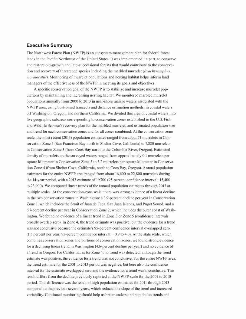
Executive SummaryThe Northwest Forest Plan (NWFP) is an ecosystem management plan for federal forest lands in the Pacific Northwest of the United States. It was implemented, in part, to conserve and restore old-growth and late-successional forests that would contribute to the conserva-tion and recovery of threatened species including the marbled murrelet (Brachyramphus marmoratus). Monitoring of murrelet populations and nesting habitat helps inform land managers of the effectiveness of the NWFP in meeting its goals and objectives.
A specific conservation goal of the NWFP is to stabilize and increase murrelet pop-ulations by maintaining and increasing nesting habitat. We monitored marbled murrelet populations annually from 2000 to 2013 in near-shore marine waters associated with the NWFP area, using boat-based transects and distance estimation methods, in coastal waters off Washington, Oregon, and northern California. We divided this area of coastal waters into five geographic subareas corresponding to conservation zones established in the U.S. Fish and Wildlife Service’s recovery plan for the marbled murrelet, and estimated population size and trend for each conservation zone, and for all zones combined. At the conservation zone scale, the most recent (2013) population estimates ranged from about 71 murrelets in Con-servation Zone 5 (San Francisco Bay north to Shelter Cove, California) to 7,880 murrelets in Conservation Zone 3 (from Coos Bay north to the Columbia River, Oregon). Estimated density of murrelets on the surveyed waters ranged from approximately 0.1 murrelets per square kilometer in Conservation Zone 5 to 5.2 murrelets per square kilometer in Conserva-tion Zone 4 (from Shelter Cove, California, north to Coos Bay, Oregon). Annual population estimates for the entire NWFP area ranged from about 16,600 to 22,800 murrelets during the 14-year period, with a 2013 estimate of 19,700 (95-percent confidence interval: 15,400 to 23,900). We computed linear trends of the annual population estimates through 2013 at multiple scales. At the conservation-zone scale, there was strong evidence of a linear decline in the two conservation zones in Washington: a 3.9-percent decline per year in Conservation Zone 1, which includes the Strait of Juan de Fuca, San Juan Islands, and Puget Sound, and a 6.7-percent decline per year in Conservation Zone 2, which includes the outer coast of Wash-ington. We found no evidence of a linear trend in Zone 3 or Zone 5 (confidence intervals broadly overlap zero). In Zone 4, the trend estimate was positive, but the evidence for a trend was not conclusive because the estimate’s 95-percent confidence interval overlapped zero (1.5 percent per year; 95-percent confidence interval: −0.9 to 4.0). At the state scale, which combines conservation zones and portions of conservation zones, we found strong evidence for a declining linear trend in Washington (4.6-percent decline per year) and no evidence of a trend in Oregon. For California, as for Zone 4, no trend was detected; although the trend estimate was positive, the evidence for a trend was not conclusive. For the entire NWFP area, the trend estimate for the 2001 to 2013 period was negative, but here also the confidence interval for the estimate overlapped zero and the evidence for a trend was inconclusive. This result differs from the decline previously reported at the NWFP-scale for the 2001 to 2010 period. This difference was the result of high population estimates for 2011 through 2013 compared to the previous several years, which reduced the slope of the trend and increased variability. Continued monitoring should help us better understand population trends and

assess underlying factors that might explain trends and variability in annual estimates. The population monitoring results to date indicate that the NWFP goal of stabilizing and increas-ing marbled murrelet populations has not yet been achieved throughout the NWFP area.
Another objective of the effectiveness monitoring plan for the marbled murrelet includes mapping baseline nesting habitat (at the start of the NWFP) and estimating changes in that habitat over time. Using maximum entropy (Maxent) models, we modeled nesting habitat suitability over lands in the murrelet’s range in Washington, Oregon, and California. The models used vegetation and physiographic attributes and a sample of 368 murrelet nest sites (184 confirmed murrelet nest sites and 184 occupied sites) for model training, and provided estimates of suitable nesting habitat for a baseline year (1993) and 20 years later (2012). We estimated that there were about 2.5 million ac of potential nesting habitat over all lands in the murrelet’s range in Washington, Oregon, and California at the start of the plan (1993). Of this total, 0.46 million ac were identified as highest suitability, matching or exceeding the average conditions for the training sites. Most (90 percent) of potential nesting habitat in 1993 on federally administered lands occurred within federal reserved-land-use allocations. A sub-stantial amount (41 percent) of baseline habitat occurred on nonfederal lands, including 44 percent of the highest suitability habitat. We found a net loss of about 2 percent of potential nesting habitat from 1993 to 2012 on federal lands, compared to a net loss of about 27 percent on nonfederal lands. For federal and nonfederal lands combined, the net loss was about 12 percent. Fire was the major cause of nesting habitat loss on federal lands since the NWFP was implemented, but timber harvest and insect damage or disease also caused losses; timber harvest was the primary cause of loss on nonfederal lands. The large amount of younger forest of lower suitability located in reserves has the potential to offset habitat losses over time, but this merits further investigation using spatially explicit forest development models.
Although the NWFP can provide nesting habitat, the marbled murrelet depends upon the marine environment to meet its foraging and roosting requirements, in addition to its use of terrestrial forest to meet its nesting requirements. To assess the relative contribu-tions of terrestrial and marine factors on murrelet abundance, distribution, and trends, we synthesized data on the status and trend of murrelet populations, inland nesting habitat, and marine factors. Specifically, we initially examined the spatial and temporal correlations of marine and terrestrial factors with the spatial distribution and trend of murrelets. We then conducted a multivariate analysis by using a boosted regression tree method to concurrently investigate the contributions of a suite of marine and terrestrial factors to at-sea murrelet abundance and trends. In both analyses, we found that numbers of murrelets are positively correlated with amounts and pattern (large contiguous patches) of suitable nesting habitat, and that population trend is most strongly correlated with trend in nesting habitat although marine factors also contribute to this trend. Model results suggest that conservation of suitable nesting habitat is key to murrelet conservation, but marine factors, especially factors that contribute to murrelet prey abundance, may play a role in murrelet distribution and trend. Conservation of habitat within reserves, as well as management actions that are designed to minimize loss of suitable habitat or improve quality of nesting habitat on all lands, should contribute to murrelet conservation and recovery.
PrefaceIn the 1980s, public controversy intensified in the Pacific Northwest over timber harvest in old-growth forests, declining species populations (such as northern spotted owl [Strix occi-dentalis caurina], marbled murrelet [Brachyramphus marmoratus], and Pacific salmon]), and the role of federal forests in regional and local economies. This ultimately led to the adoption of the Northwest Forest Plan (NWFP), which amended existing management plans for 19 national forests and 7 Bureau of Land Management districts in California, Oregon, and Washington (24 million ac of federal land within the 57-million-ac range of the north-ern spotted owl). The NWFP provides a framework for an ecosystem approach to the man-agement of those 24 million ac of federal lands. It established the overarching conservation goals of (1) protecting and enhancing habitat for species associated with late-successional and old-growth forests, (2) restoring and maintaining the ecological integrity of watersheds and aquatic ecosystems, and (3) providing a predictable level of timber sales and other services, as well as maintaining the stability of rural communities and economies.
The NWFP relies on monitoring to detect changes in ecological and social systems relevant to its success in meeting conservation objectives, and on adaptive management processes that evaluate and use monitoring information to adjust conservation and manage-ment practices (Mulder et al. 1999). An interagency effectiveness monitoring framework was implemented to meet requirements for tracking status and trend for watershed condi-tion, late-successional and old-growth forests, social and economic conditions, tribal rela-tionships, and population and habitat for marbled murrelets and northern spotted owls. This report is one of a set of status and trend monitoring reports on these topics that addresses questions about the effectiveness of the NWFP in meeting its objectives through its first 20 years. Monitoring results for the first 10 years and first 15 years are documented in a series of reports available online at http://www.reo.gov/monitoring/reports/index.shtml.
This is the third in a series of monitoring reports from the Marbled Murrelet Effec-tiveness Monitoring module under the NWFP, and focuses on monitoring results on the status and trends for marbled murrelet populations and nesting habitat through the first 20 years of the NWFP (1994–2013), following the design described in Marbled Murrelet Effectiveness Monitoring Plan for the Northwest Forest Plan (Madsen et al. 1999). This report is composed of three chapters. Chapter 1 discusses the status and trend of the portion of the murrelet population associated with the NWFP area. Chapter 2 presents the status and trend of murrelet nesting habitat. Chapter 3 presents results from an evaluation of the relationships between murrelet distribution at sea off the NWFP area, nesting habitat dis-tribution and other terrestrial factors, and marine factors. This chapter is a first step toward meeting the long-term monitoring goal of the murrelet monitoring strategy, as described in Madsen et al. (1999), of developing a predictive model that relates forest habitat conditions to the demographic health of the murrelet population. In addition, chapter 3 provides a brief synthesis of the results of all three chapters, and a discussion of management implications of these results.
Literature CitedMadsen, S.; Evans, D.; Hamer, T.; Henson, P.; Miller, S.; Nelson, S.K.; Roby, D.;
Stapanian, M. 1999. Marbled murrelet effectiveness monitoring plan for the Northwest Forest Plan. Gen. Tech. Rep. PNW-GTR-439. Portland, OR: U.S. Department of Agriculture, Forest Service, Pacific Northwest Research Station. 51 p.
Mulder, B.S.; Noon, B.R.; Spies, T.A.; Raphael, M.G.; Palmer, C.J.; Olsen, A.R.; Reeves, G.H.; Welsh, H.H., Jr. 1999. The strategy and design of the effectiveness monitoring program for the Northwest Forest Plan. Gen. Tech. Rep. PNW-GTR-347. Portland, OR: U.S. Department of Agriculture, Forest Service, Pacific Northwest Research Station. 138 p.


Contents 1 Chapter 1: Status and Trend of Marbled Murrelet Populations in the Northwest
Forest Plan AreaGary A. Falxa, Martin G. Raphael, Craig Strong, Jim Baldwin, Monique Lance,
Deanna Lynch, Scott F. Pearson, and Richard D. Young 1 Summary 2 Introduction 3 What Is New Since Publication of the 15-Year Report? 3 Methods 3 Sampling Design 6 Analysis 13 Results 13 Population Estimates 17 Trend Analyses 24 Discussion 26 Trend Pattern 27 Sampling and Interpretation Challenges 29 Potential Uncertainties in Sampling 30 Potential Causes for Decline 31 Acknowledgments 32 References 37 Chapter 2: Status and Trend of Nesting Habitat for the Marbled Murrelet Under
the Northwest Forest PlanMartin G. Raphael, Gary A. Falxa, Deanna Lynch, S. Kim Nelson, Scott F. Pearson,
Andrew J. Shirk, and Richard D. Young 37 Summary 37 Introduction 38 Methods 38 Analytical Methods 39 Study Area 39 Land Use Allocations 42 Data Sources for Covariates 45 Other Data Sources 46 Covariate Selection and Screening 46 Accuracy Assessment 46 Data Preparation 48 Murrelet Locations 49 Habitat Change 49 LandTrendr Change Detection 51 Model Refinements 52 Summarizing Maxent Output 55 Landscape Habitat Pattern—Edge Versus Core 56 Human Disturbance 56 Results
56 Covariates 63 Model Performance 65 Habitat Suitability 72 Habitat Change 77 Habitat Pattern 82 Human Disturbance 82 Discussion 82 Sources of Uncertainty 85 Interpretation of Model Output 85 Comparison With Previous Estimates 86 Implications of Results 87 Acknowledgments 87 References 95 Chapter3:FactorsInfluencingStatusandTrendofMarbledMurreletPopula-
tions: An Integrated PerspectiveMartin G. Raphael, Andrew J. Shirk, Gary A. Falxa, Deanna Lynch, S. Kim Nelson,
Scott F. Pearson, Craig Strong, and Richard D. Young 95 Summary 95 Introduction 96 Methods 96 Univariate Correlations 98 Multivariate Model 101 Results 101 Spatial Correlations 104 Temporal Correlations 106 Multivariate Model 111 Discussion 111 Spatial Variation 111 Temporal Variation 112 Multivariate Model 112 Effects of Climate 113 Management Implications 115 Summary Conclusions 116 Acknowledgments 116 References 121 Appendix 1: Power Analysis 121 Introduction 121 Methods 123 Results 123 Power to Detect Trends 124 References 125 Appendix 2: Field Audit Form 127 Appendix 3: Population Estimates at Stratum Scale, With Distance Parameters

1
Status and Trend of Marbled Murrelet Populations and Nesting Habitat
Chapter 1: Status and Trend of Marbled Murrelet Populations in the Northwest Forest Plan AreaGary A. Falxa,1 Martin G. Raphael,2 Craig Strong,3 Jim Baldwin,4 Monique Lance,5 Deanna Lynch,6 Scott F. Pearson,7 and Richard D. Young8
SummaryThe Northwest Forest Plan (NWFP) is an ecosystem management plan for federal forest lands in the Pacific Northwest of the United States. It incorporates a program to monitor the effectiveness of the NWFP in meeting various objectives, including supporting populations of species associated with late-successional and old-growth forests. To evaluate the NWFP’s effectiveness in conserving species associated with older forests, we monitored marbled murrelet (Brachyramphus marmoratus) populations annually from 2000 to 2013 in near-shore marine waters associated with the NWFP area. We counted murrelets along transect lines using boats in coastal waters off Washington, Oregon, and northern California (north of San Francisco Bay) and used distance estimation methods to account for detectability. We divided this area of coastal waters into five geographic subareas corresponding to conservation zones established in the U.S. Fish and Wildlife Service’s recovery plan for the marbled murrelet, and estimated population size and trend for each conservation zone, and for all zones combined. At the conservation-zone scale, the most recent (2013) population estimates ranged from about 71 murrelets in Conservation Zone 5 (San Francisco Bay north to Shelter Cove, California) to 7,880 murrelets in Conservation Zone 3 (from Coos Bay,
Oregon, north to the Columbia River). The density estimates ranged from to 0.1 murrelets per square kilometer in Con-servation Zone 5 to 5.2 murrelets per square kilometer in Conservation Zone 4 (from Shelter Cove, California, north to Coos Bay, Oregon). Annual population estimates for the entire NWFP area ranged from about 16,600 to 22,800 murrelets during the 14-year period, with a 2013 estimate of 19,700 (95-percent confidence interval: 15,400 to 23,900). We assessed for potential linear trends of the annual population estimates through 2013 at the NWFP-wide (all five conserva-tion zones), single-zone, and state scales. At the scale of the individual conservation zone, there was strong evidence of a linear decline in the two conservation zones in Washington: a 3.9-percent decline per year (95-percent confidence interval: −7.6 to 0) in Conservation Zone 1, which includes the Strait of Juan de Fuca, San Juan Islands, and Puget Sound; and a 6.7-percent decline per year (95-percent confidence interval: −11.4 to −1.8) in Conservation Zone 2, which includes the outer coast of Washington. In contrast, we found no evidence of a linear trend in Zone 3 or Zone 5 (confidence intervals broadly overlap zero). In Conservation Zone 4, the trend estimate was positive, but the evidence for a trend was not conclusive because the estimate’s 95-percent confidence interval overlapped zero (1.5 percent per year; 95-percent confidence interval: −0.9 to 4.0). At the state scale, which combines conservation zones and portions of conservation zones, we found strong evidence for a declining linear trend in Washington (4.6-percent decline per year; 95-percent confidence interval: −7.5 to −1.5 percent) and no evidence of a trend in Oregon. For California, as for Zone 4, no trend was detected; although the trend estimate was positive, the evidence for a trend was not conclusive (+2.5 percent per year; 95-percent confidence interval: −1.1 to 6.2). No trend was detected for the overall NWFP area; although the trend estimate was negative, the evidence was not conclusive (−1.2 percent per year; 95-percent confidence interval: −2.9 to 0.5) over the 2001 to 2013 period. The NWFP-area trend for this period differs from the decline previously observed for the
1 Fish and wildlife biologist, U.S. Fish and Wildlife Service, Arcata Fish and Wildlife Office, 1655 Heindon Rd., Arcata, CA 95521.2 Research wildlife biologist, U.S. Department of Agriculture, Forest Service, Pacific Northwest Research Station, 3625 93rd Ave. SW, Olympia, WA 98512.3 Consultant researcher, Crescent Coastal Research, 7700 Bailey Road, Crescent City, CA 95531.4 Statistician unit leader, U.S. Department of Agriculture, Forest Service, Pacific Southwest Research Station, 800 Buchanan Street, West Annex Building, Albany, CA 94710.5 Research biologist, Washington Department of Fish and Wildlife, 7801 Phillips Road SW, Lakewood, WA 98498.6 Fish and wildlife biologist, U.S. Fish and Wildlife Service, Wash-ington Fish and Wildlife Office, Branch of Listing, 510 Desmond Dr., Suite 102, Lacey, WA 98503.7 Senior research scientist, Washington Department of Fish and Wildlife, 1111 Washington Street SE, Olympia, WA 98501.8 Geographic information system analyst, U.S. Fish and Wildlife Service, Pacific Regional Office, Ecological Services, 911 NE 11th Ave. Portland, OR 97232.
2
GENERAL TECHNICAL REPORT PNW-GTR-933
2001 to 2010 period. This difference was the result of high population estimates for 2011 through 2013 compared to the previous several years, which reduced the slope of the trend and increased variability. Contributing to the recent high NWFP-area estimates were higher estimates in Conservation Zone 1 in 2011 and 2012, and in Conservation Zones 3 and 4. Continued monitoring should help us to better understand population trends and to assess underlying factors that might explain trends and variability in annual estimates. The population monitoring results indicate that the NWFP goal of stabilizing and increasing marbled murrelet populations has not yet been achieved; potential causes for this are discussed in chapter 3.
IntroductionEstablished in 1994, the NWFP represented a major change in how federal forest lands are managed in western Wash-ington, western Oregon, and northwest California. It was developed in response to public controversy during the late 1980s and early 1990s over the harvest of old forests on federal lands. Although public concerns included the loss of old-growth forest ecosystems as a whole, the controversy was fueled and focused in part by concern about the impacts of harvest activities on the northern spotted owl (Strix occidentalis caurina), which was listed in 1990 as threat-ened under the federal Endangered Species Act (USFWS 1990). In 1992, the marbled murrelet, a seabird dependent on old-growth forests for nesting habitat, was also listed as threatened in Washington, Oregon, and California (USFWS 1992). For both species, loss and degradation of habitat from timber harvesting, exacerbated by catastrophic events including fire and windstorms, were the primary factors contributing to these listings (USFWS 1990, 1992).
The NWFP provides a framework for an ecosystem approach to the management of about 10 million ha (24.5 million ac) of federal lands within the range of the northern spotted owl (USDA and USDI 1994). It established the over-arching conservation goals of (1) protecting and enhancing habitat for species associated with late-successional and old-growth forests, (2) restoring and maintaining the ecological integrity of watersheds and aquatic ecosystems, and (3) providing a predictable level of timber sales and
other services, as well as maintaining the stability of rural communities and economies. A more specific conservation goal of the NWFP is to stabilize and increase marbled murrelet populations by maintaining and increasing nesting habitat (Madsen et al. 1999). The NWFP (USDA and USDI 1994) identified the following as a primary question for evaluating the plan’s effectiveness in achieving this goal: Is the marbled murrelet population stable or increasing? This chapter will address this question based on data collected during the NWFP’s first 20 years.
Ecological monitoring programs were established to evaluate the effectiveness of the NWFP in meeting con-servation objectives, and to inform management decisions (Mulder et al. 1999). Specifically, monitoring programs were established to assess the status and trends of (1) late-successional and old-growth forests, (2) northern spotted owl habitat and populations, (3) marbled murrelet habitat and populations, (4) federal agency relationships with Indian tribes, (5) watershed conditions, and (6) socioeco-nomic conditions.
Although the marbled murrelet is a seabird that spends most of its time living and foraging in coastal marine waters, it was selected for monitoring because it is strongly associated with late-successional and old-growth forests for nesting (Madsen et al. 1999). It nests mostly on large branches or other suitable platforms in large coniferous trees (Nelson 1997, Ralph et al. 1995). Nesting habitat is key to marbled murrelet conservation (Piatt et al. 2007; Ralph et al. 1995; Raphael 2006; USFWS 1997, 2009). Owing mainly to timber harvesting, only a small percentage (5 to 20 percent, depending on region) of original old-growth forest remains (Morrison 1988; Norheim 1996, 1997), mostly in relatively small, fragmented patches or in forest parks and reserves. The NWFP identified several goals for marbled murrelet nesting habitat, including providing substantially more suit-able habitat for marbled murrelets than existed at the start of the plan, providing large contiguous blocks of murrelet nest-ing habitat, and improving or maintaining the distribution of populations and habitat (Madsen et al. 1999). Monitoring murrelet population trends provides a key indicator of whether the NWFP is successfully providing nesting habitat to support a stable and well-distributed murrelet population
3
Status and Trend of Marbled Murrelet Populations and Nesting Habitat
(Madsen et al. 1999); chapter 2 of this report provides results from the monitoring of nesting habitat.
Marbled murrelet monitoring for the NWFP includes both habitat and population components (Madsen et al. 1999). For habitat monitoring, the approach is to establish a baseline level of nesting habitat by first modeling habitat relationships, and then comparing habitat changes to the baseline (Huff et al. 2006; Raphael et al. 2006, 2011). Popu-lation size and trends are monitored using a unified sampling design and standardized survey methods (Miller et al. 2006, 2012; Raphael et al. 2007). Thus, trends in both murrelet nesting habitat and populations are tracked over time. The ultimate goal is to relate population trends to the amount and distribution of nesting habitat (Madsen et al. 1999).
What Is New Since Publication of the 15-Year Report?In this report, the status and trend analyses incorporate several more years of sampling data, through 2013. Although methods have remained consistent for murrelet population monitoring, we also conducted a number of new analyses, including:• An extensive review of all data 2000 to 2013 for
consistency and archival purposes, followed by a reanalysis of the density, size, and trends of murrelet populations associated with the NWFP area
• A new analysis of the effect of Beaufort sea state on the detectability of murrelets, and thus on estimated murrelet densities and trends throughout the analysis area, at multiple spatial scales
• An evaluation of whether murrelet distribution with respect to distance from shore (inshore versus off-shore subunit) changed over the 2000 to 2013 period
• An evaluation of state-level population status and trends, for use by state managers and others (e.g., evaluating state-level recovery); this is in addition to the ongoing analysis of status and trends at the con-servation zone and NWFP area scales.
• An updated power analysis using sampling data through 2013 to forecast the program’s ability to detect trends in future surveys under a reduced mon-itoring effort.
MethodsSampling DesignThe objectives of our murrelet population monitoring are to estimate population size and trend in coastal waters adjacent to the NWFP area, which extends from the United States border with British Columbia south to the Golden Gate of San Francisco Bay (fig. 1-1). The NWFP area encompasses five of the six marbled murrelet conservation zones (sampling strata) designated by the Marbled Murrelet Recovery Plan (USFWS 1997). The target population is also defined by the area of navigable waters within from 3 to 8 km of shore (distance varies by conservation zone), and temporally from mid-May through the end of July, when breeding murrelets at sea are likely to be associated with inland nesting habitat. The total area of coastal waters within this area and containing the target population was about 8785 km2 (3,392 mi2). Within each conservation zone (fig. 1-1), two or three geographic strata were des-ignated based on patterns of murrelet density (Miller et al. 2006, Raphael et al. 2007). The distance from shore of the offshore boundary for the target population varied among conservation zones and strata, and was selected in each area to capture at least 95 percent of the murrelets on the water (Bentivoglio et al. 2002; Miller et al. 2006, 2012; Raphael et al. 2007). Sampling was designed to allocate more effort to strata with higher murrelet densities (Raphael et al. 2007).
To assess murrelet density and population size within each conservation zone and stratum, we established Pri-mary Sampling Units (PSU) that are roughly rectangular areas of about 20 km of coastline and are contiguous over the entire sampling area. The PSU and strata boundaries remained constant over the sampling period. Each conser-vation zone includes from 14 to 22 unique PSUs, except for Conservation Zone 1, where the complex shoreline of the Puget Sound area resulted in 98 PSUs. Although the NWFP was implemented in 1994, it took several years to develop an effectiveness monitoring plan and sampling design. Following completion of the effectiveness moni-toring plan for murrelets (Madsen et al. 1999), population monitoring began in 2000 for all conservation zones. Our target sample size in Conservation Zones 2 through 5 was
4
GENERAL TECHNICAL REPORT PNW-GTR-933
o0 200
Miles
Zone 5
Zone 4
Zone 3
Zone 2
Zone 1
Oregon
California
Washington
Figure 1-1—The five at-sea marbled murrelet survey (conservation) zones adjacent to the Northwest Forest Plan (NWFP) area. The shaded area corresponds to the overlap between the NWFP area and the approximate breeding distribution of the murrelet. See figure 1-4 for the offshore boundaries of the marine waters sampled (adapted from USFWS 1997).
5
Status and Trend of Marbled Murrelet Populations and Nesting Habitat
30 PSU surveys per conservation zone per year; most or all unique PSUs in these conservation zones were sampled each year and in a random sampling order. In Conservation Zone 1, an initial sample of 30 PSUs was randomly selected out of the 98 available PSUs, and each selected PSU was sampled twice each year (Raphael et al. 2007). This same random Conservation Zone 1 subsample was sampled each year to minimize between-year variance. In Conservation Zone 5, the target sample was reduced to 15 PSUs in 2004 to balance logistics, cost and precision in this area of very few murrelets. Conservation Zone 5 was not sampled in 2006, 2009, 2010, or 2012 owing to funding limitations. We discuss below, in the section “Treatment of Years With No Surveys for Conservation Zone 5,” how we dealt with missing data from Conservation Zone 5 in population size and trend estimates.
We divided PSUs into inshore and offshore subunits (fig. 1-2), which allows more sampling effort in nearshore subunits with higher murrelet density (Bentivoglio et al. 2002). However, PSUs in stratum 3 of Conservation Zone 1 were not
divided into subunits, as murrelet density was low throughout the stratum. The inshore unit extended to either 1500 or 2000 m from shore, except in stratum 2 of Conservation Zone 1, where narrow inlets and passages between opposite shore-lines limited the inshore subunit to within 500 m of shore. As discussed below, for Conservation Zone 5 we changed the division between inshore and offshore PSU subunits in 2005 from 2000 m offshore to 1200 m. Inshore PSU sub-units generally have higher murrelet densities, so they were sampled with more effort using transects placed parallel to shore. Offshore PSU subunit transects are oriented diagonally with the shoreline, often in a zigzag configuration (fig. 1-2) to sample across the gradient of murrelet density that, generally, declines with distance from shore (Ralph and Miller 1995). The PSU sampling details for each conservation zone and stratum are summarized in Raphael et al. (2007).
We use two observers for each survey, one on each side of the boat’s centerline, surveying a 90° arc to the left or right of the bow, but emphasizing the area in front of the boat. We estimated murrelet density using line transect
Offshore
Inshore
2 to 8 km (distance varies by zone)
D C B A
5 km (each) segments
Su
bu
nit
s
Figure 1-2—Marbled murrelet primary sampling unit with inshore and offshore subunits showing parallel and zigzag transects. The inshore subunit is divided into four equal-length segments (approximately 5 km each) and four equal-width bins (bands parallel to and at increasing distances from shore). One bin is selected without replacement (depicted by heavier line) for each segment of transect.

6
GENERAL TECHNICAL REPORT PNW-GTR-933
methods (Buckland et al. 2001, Thomas et al. 2004), where the perpendicular distance to each detected murrelet or group of murrelets was estimated. Accuracy of distance estimates is key to density estimates using line transect methods. Distance training and calibration occurred throughout the season to maintain consistency in distance estimates between observers and across years. Because surface waves can obscure murrelets on the water, observers noted sea state using the Beaufort scale. The Beaufort scale is an empirical measure that relates windspeed to observed conditions at sea, ranging from a value of 0 (calm, flat sea conditions) to 12 (hurricane-force winds). Surveys were generally conducted under sea conditions of Beaufort 2 or less, although occasion-ally surveys continued after conditions increased to Beaufort 3. Description of the complete survey protocol is provided in Raphael et al. (2007) and in Miller et al. (2006). Minor adjust-ments to the survey protocol are described below in “Protocol Clarifications and Refinements.” In addition to recording all marbled murrelet detections, observers also recorded other seabirds and marine mammals detected during sampling.
Using this protocol, we conducted population mon-itoring surveys in the five conservation zones beginning in 2000, and sampled all conservation zones except Con-servation Zone 5 in each year between 2000 and 2013. In any year, we conducted 150 to 200 PSU surveys across all conservation zones combined, and recorded approximately 4,000 to 6,000 marbled murrelet observations along roughly 5500 to 6500 km of transect (table 1-1). Because some PSUs are sampled more than once in a year, the number of unique PSUs sampled annually is about 90 to 95 PSUs across the five conservation zones (Raphael et al. 2007).
AnalysisDensity and population estimates—We conducted surveys from 2000 through 2013. Departures from the protocol in Conservation Zones 1 and 2 in 2000 may have affected density estimates for those conservation zones. Therefore we used data from only 2001 through 2013 for all estimates and analyses involving these conservation zones, namely those for Conservation Zone 1, Conservation Zone 2, Washington State, and “All-Zones” (the five con-servation zones combined). Conservation Zone 5 was not
sampled in four of the years (2006, 2009, 2010, and 2012), and we interpolated Conservation Zone 5 densities for those years based on data from adjacent years and methods described below (see “Treatment of Years With No Surveys in Conservation Zone 5”).
For each year of survey, we estimated average marbled murrelet densities (murrelets per square kilometer), with an associated estimate of precision for each conservation zone, for the entire target population, and for the three states within the area sampled. We used distance sampling methods (Buckland et al. 2001, 2004) and the software program DISTANCE version 6.2 (Thomas et al. 2010) to estimate the probability for detecting a murrelet that is present at distance zero [ f(0)] and the mean number of murrelets per group [or cluster size; E(s)] for each year and conservation zone from inshore and offshore subunit surveys. We truncated the distance data prior to analysis by discarding the 5 percent of observations with the greatest distances for each conservation zone, which can improve modeling of detection functions, as recommended by Buckland et al. (2001). We set DISTANCE to use the mean observed cluster size as the estimate for E(s) unless an internal test found evidence that detection is a function of cluster size, in which case DISTANCE applied a correction (Buckland et al. 2001). For each year, the data from Conser-vation Zones 4 and 5 were combined for estimating the detection function, E(s), f(0), and truncation distance. We did this because the low number of murrelet detections in Conservation Zone 5 was insufficient for estimating these parameters. DISTANCE also provided the number of groups of murrelets observed per kilometer (ER = encounter rate) for each PSU subunit survey. We then estimated density (murrelets/square kilometer) for each PSU subunit survey (Raphael et al. 2007) using the estimates and encounter rate from DISTANCE with the following formula:
The “hats” over the letters designate estimates. Strata, conservation zone, and All-Zones density estimates were constructed from average densities weighted by the area of the respective geographic scale.
d = 1000 × ƒ (0) × E (s) × ER 2
ˆ ˆ ˆ
7
Status and Trend of Marbled Murrelet Populations and Nesting Habitat
Table 1-1—The number of marbled murrelet population monitoring primary sampling unit (PSU) surveys completed for the Northwest Forest Plan, and the total kilometers of survey transect sampled from 2000 to 2013
Year Zone Number of PSU surveys Survey effortKilometers
2000 1 N/A N/A2 N/A N/A3 24 10024 57 14935 29 792
2001 1 60 21582 22 10393 27 10674 54 14215 22 602
2002 1 60 22282 22 9833 31 12394 56 13975 26 705
2003 1 60 22102 30 13593 30 11324 55 14185 19 508
2004 1 57 21332 30 13753 30 11884 32 8365 16 412
2005 1 60 22342 26 11363 28 11084 31 8125 15 432
2006 1 60 22302 29 13003 31 11854 30 7765 No surveys
Year Zone Number of PSU surveys Survey effortKilometers
2007 1 60 22132 31 14293 30 11514 29 7505 14 423
2008 1 60 22352 31 14413 30 11224 31 8025 13 385
2009 1 60 22302 31 13803 31 11114 35 9125 No surveys
2010 1 60 22462 30 13423 30 11694 26 6765 No surveys
2011 1 60 22222 30 13563 31 12014 32 8135 16 469
2012 1 60 22312 34 15673 29 11684 27 7025 No surveys
2013 1 60 22462 30 13613 29 11594 31 8085 15 454
N/A = not applicable.

8
GENERAL TECHNICAL REPORT PNW-GTR-933
Target population estimates for each conservation zone and for the five conservation zones combined were produced using standard methods for stratified sampling (Cochran 1977, Sokal and Rohlf 1981). We used the total area within each stratum to expand the density estimates from DISTANCE, and associated estimates of precision, to calculate the average total numbers of murrelets by conservation zone, state, and for all conservation zones combined for the target period. Estimates of precision were produced using bootstrap resam-pling methods with consideration of PSU samples that might be clustered in time or space (Miller et al. 2006, Raphael et al. 2007). Density and population estimates were equivalent for purposes of trend analysis because the total area (area sampled) was constant over the study for all conservation zones, and because population is simply a multiple of density. Details on methods used to calculate population estimates and confidence intervals are provided in Raphael et al. (2007).
To portray variation in at-sea density at a finer scale, we obtained a mean density at the PSU scale by first averaging the annual density for each PSU at two scales: the entire PSU, and for the separate inshore and offshore subunits. We then calculated the mean density for each PSU and its subunits by averaging the annual values throughout the sample period.
Estimating trends—We assessed for linear trends in murrelet density in the NWFP area from 2000 through 2013, excluding the year 2000 from analyses that involved Conservation Zones 1 and 2, as previously noted. We estimated trends for each conservation zone, for All-Zones, and for each state. For Conservation Zone 5, the single-conservation zone trend analysis used data from all years with surveys from 2000 through 2013; for the All-Zones analyses, we used the interpolated Conservation Zone 5 densities for the years not sampled (2006, 2009, 2010, and 2012). Because Conservation Zone 5 supports less than one percent of the target population, missing data had very little effect on population estimates and no measurable influence on trend magnitude or significance; this was confirmed empirically by analyzing trends for the NWFP area with and without Conservation Zone 5 included.
We fit a linear regression to the natural logarithm of annual density estimates to test for declining trends in individual Conservation Zones 1 through 5 and in All-Zones. For our analysis, the natural logarithm best fits and tests existing demographic models (McShane et al. 2004, USFWS 1997) that predicted a constant declining murrelet population. We tested the null hypothesis that the slope equals zero or greater (no change or increase in murrelet numbers) against the alternative hypothesis of the slope being less than zero (i.e., a two-tailed test for decreasing murrelet densities). In a model where the percentage of change r is constant from year to year, and d represents the murrelet density estimate in a given year:
and when we take the natural logarithm of both sides, we end up with a standard linear model:
where a and b are constants to be estimated, and error ~ N(0,σ2). Under such a model, the percentage of change from year to year is constant and is equal to r = 100(eb – 1).
For the purposes of evaluating the evidence for a linear trend, we considered (1) the magnitude of the annual trend estimate, particularly in relation to zero, where zero rep-resents a stable population, and (2) the width and location of the 95-percent confidence intervals surrounding that trend estimate, also in relation to zero. The evidence for a popula-tion trend, versus a stable population, is stronger when the trend estimate and its 95-percent confidence interval do not overlap zero, and when the trend estimate is farther from zero. When the confidence interval of a trend estimate is tight around zero, then we would conclude that there is no evidence of a trend. Finally, when the confidence interval of a trend estimate broadly overlaps zero and the trend estimate is not close to zero, this indicates evidence that is not conclusive for or against a non-zero trend. Confidence intervals that are mainly above or below zero, but slightly overlap zero, can provide some evidence of a trend.
d Year = d 2000 × 1 + Year – 2000
× eerror r
100
(Year – 2000) + error × (Year – 2000) + error
log(d Year) = log(d 2000) + log 1 + r
100

9
Status and Trend of Marbled Murrelet Populations and Nesting Habitat
To illustrate the cumulative, multiyear effect on population size of the annual population trend estimates from our analyses, we calculated for each trend estimate the cumulative population change over a 10-year period during the period of sampling. For this calculation, we defined a 10-year period as one encompassing 10 increments of change at the annual rate, such as the time period 2003 to 2013. Our calculation used the following formula, where R is the estimated annual percentage rate of change:
The cumulative change value assumes a constant rate of change at the estimated trend rate, based on an exponential model of population change.
Effects of sea conditions on density and trend estimates—We evaluated the influence of sea conditions (Beaufort sea state) during surveys on detection functions and ultimately on density and trend estimates.
We treated the Beaufort values for each observation (typically 0, 1, or 2, occasionally 3, and rarely 4) as a categorical rather than continuous variable, because we do not know if the change in detectability at any dis-tance changes in the same amount going from Beaufort 0 to Beaufort 1 as it would be going from Beaufort 2 to Beaufort 3. Using the Distance methods previously described, we obtained separate detection curves for each Beaufort category, which along with the encounter rate and mean group size were used in Distance to estimate murrelet density. We then compared the densities of the default no-covariate model with those from the model with the sea condition covariate. In some years and conservation zones, there were too few detections within a particular Beaufort class to meet the Distance method recommendation (Buckland et al. 2001) of an average of at least three detections per distance class for modeling detection curves. In this situation, we pooled values in adjacent Beaufort classes. This resulted in the merging of Beaufort class 3 into class 2 observations (12 instances), merging Beaufort class 4 into class 3 (five instances) or class 2 (two instances), merging Beaufort class 0 obser-
vations into class 1 (six instances), and merging Beaufort class 2 into class 1 (one instance). As in other analyses, we pooled Conservation Zone 5 data with Conservation Zone 4 data, because of too few murrelet detections in Conservation Zone 5.
We used AIC methods (Johnson and Omland 2004) to identify the best model for each year, conservation zone, and Beaufort category combination, and also compared the variance in density estimates for competing models. We evaluated the effect of the sea condition covariate on the population-trend estimates by using the regression methods described above to compare the trend estimated from the density estimates provided by the no-covariate and Beaufort covariate models for each conservation zone.
Our at-sea observations are expected to have a detection probability of 1 at zero distance from the transect line and then to decline (with no subsequent increases) with increasing distance from the line; i.e., they are assumed to be monotonic and to be bounded by zero and one. When we included the sea-state covariate in our model, the program Distance would not always use a monotonic detection function, owing to inclusion of the cosine adjustment, and some estimates of probabilities exceeded 1 at some distances from the line. Cosine adjustments are intended to allow more flexibility in fitting the detection function to the observed data. However, where detection probabilities exceed one, the resulting estimate of density can be erroneous and vastly different from estimates not using Beaufort as a covariate. To address this issue, we examined Beaufort models with and without cosine adjustments for each zone-year combination. Between the two models, we selected the Beaufort model with the smallest AICc value, except when the model with the cosine adjust-ment produced an estimated detection probability greater than 1, in which case we used the “no cosine adjustment” Beaufort model results.
In three cases (2001 for Conservation Zone 1 and 2001 and 2002 for Conservation Zone 2), sea- condition data were not available, so these conservation zone-year combinations were excluded from the analysis.
We previously evaluated and reported on potential observer (crew) effects with a subset of data (Miller et al. 2012) and did not repeat that evaluation for this report.
Cumulative change (%) = 100 1 + – 1 R
100
10
10
GENERAL TECHNICAL REPORT PNW-GTR-933
Power analysis—We conducted a new power analysis, based on population monitoring data through 2013. The goal of this analysis was to examine the power to detect trends under the reduced sampling effort, which we initiated in 2014. The methods and results from this new power analysis are fully reported in appendix 1.
Temporal and spatial variation in marbled murrelet distribution as a function of distance from shore—During the planning phase of the monitoring program, researchers subdivided each PSU into inshore and offshore subunits, to allow allocation of greater sampling effort to inshore areas, where densities of murrelets tend to be greater (Raphael et al. 2007). The allocation of effort was based on data collected prior to 2000, and subject to future adjustment based on new data (Bentivoglio et al. 2002, Raphael et al. 2007). We calculated and inspected the ratios of inshore to offshore density for each year-conservation zone combination to evaluate whether those ratios support the protocol’s current allocation of greater sampling effort nearshore. Ratio values >1.0 indicate a greater density of murrelets in the inshore subunits relative to the offshore.
We also evaluated whether the ratio of inshore density to offshore density changed in a consistent manner over time during the years of sampling through 2013. If such changes were observed, then that would trigger a reconsideration of the current allocation of total survey length between the inshore and offshore subunits within PSUs. We conducted this analysis at the stratum scale, the minimum scale at which the survey design allows adjustment of survey effort alloca-tion between subunits. Using all years of survey data through 2013, we calculated the average annual density in the inshore and offshore subunits analyses at the scale of the two or three strata within each conservation zone. This provided sample sizes of about 30 to 55 PSU samples for each subunit per year. Conservation Zone 5 was excluded from this analysis because the data include many density estimates of zero. Stratum 3 of Conservation Zone 1 was also excluded from the analysis, as PSUs within this stratum do not have an offshore subunit. For each PSU stratum, we visually looked for patterns suggesting a systematic change between 2000 and 2013 in murrelet distribution as a function of distance from shore.
A change in distribution might have implications for any trend patterns observed. In particular, if a shift in murrelet distribution resulted in a smaller proportion of the population occurring within our sample area (and thus being sampled) in the latter years of this study, this might lead to underestimates of population size in those years and an erroneous decline signal. Our analysis of inshore-to-offshore density does not provide a rigorous test for such a shift. However, if we were to observe a higher proportion of murrelets offshore in the later years of this study, this could be consistent with such a shift in distribution. Similarly, should we observe no change in the nearshore/offshore ratio over time, this would lend some support to such a shift not occurring.
Protocolclarificationsandrefinements—The field and analytical methods used in the marbled mur-relet population monitoring have been presented in detail elsewhere (Raphael et al. 2007). In this section, we docu-ment several clarifications and refinements of the methods and protocol described in that publication.
Estimates of population size and trend at state scale—In this report, we include for the first time estimates of marbled murrelet population size and trend at the state scale, because this scale is relevant for evaluating conser-vation actions and regulations at that scale. We used the same analytic approach as described above, except that we calculated average annual murrelet densities for each of the three states within the sample area: Washington, Oregon, and California. We calculated average densities by weighting the murrelet density for each conservation zone, or portion thereof, within a state, by the area of coastal waters sampled within that conservation zone or portion of conservation zone. For Washington, this involved the weighted average density for Conservation Zones 1 and 2. The Oregon estimate averaged the density for Conservation Zone 3, and for the portion of Conservation Zone 4 within Oregon (PSUs 1 through 9); PSU 9 spans the Oregon-California border, but is predominately in Oregon. The California estimate averaged the density for the California portion of Conservation Zone 4 (PSUs 10 through 22) and all of Conservation Zone 5. Our California estimate does
11
Status and Trend of Marbled Murrelet Populations and Nesting Habitat
not include murrelets occurring in Conservation Zone 6 (south of the Golden Gate of San Francisco Bay), because Conservation Zone 6 is outside of the NWFP area, and thus is not sampled by this program.
Treatment of years with no surveys in Conservation Zone 5— Conservation Zone 5 was not surveyed in 4 years: 2006, 2009, 2010, and 2012. We instituted measures to formalize treatment of missing Conservation Zone 5 data in our analy-ses, which have been applied to the entire dataset. For regressions used to estimate trend for Conservation Zone 5, we use only data from years with surveys. For All-Zones population and density estimates and trend analyses, we used interpolation methods. When Conservation Zone 5 has been sampled both before and after the year without surveys (as is the case for all years in this report), we use mean of the prior and following year densities to estimate the missing year’s density. If Conservation Zone 5 is not surveyed for 2 consecutive years, as occurred in 2009–2010, we interpolate using the prior and following years with surveys. For example, for 2009 and 2010, we estimated density (d ) using 2008 and 2011 Conservation Zone 5 data and the following formula:
When Conservation Zone 5 was not surveyed in the last year of analysis period, we use data from the most recent prior year with Conservation Zone 5 surveys to extrapolate density for the missing data.
We also used the interpolated values for Conservation Zone 5 in our “All-Zones” trend estimate. We estimated the “All-Zones” density and standard error of density using the following formulas, where az is the area of Conserva-tion Zone Ζ:
Adjusted boundary separating inshore and offshore subunits in Conservation Zone 5—In early 2005, we used the 2000–2004 data to review murrelet distribution as a function of distance from shore. This review indicated that most murrelets were observed within 1300 m of shore. As a result, we adjusted the location of the boundary separating the inshore and offshore subunits from 2000 m offshore to 1200 m offshore. By reducing the area of the inshore subunit while maintain-ing the same survey effort in that subunit, we increased survey effort to that area of higher density. Concurrently, the length of the offshore effort increased from about 6 km to about 9 km per PSU sample. The adjusted length of the offshore transect was calculated using the following formula (details in Raphael et al. 2007):
where the ratio (r) of the optimal inshore to offshore transect length (which minimizes the variance of the PSU density estimator) is based on the mean densities in the two subunits (d1 and d2) and the area of the subunits (a1 and a2) when a Poisson distribution is assumed for the observed counts. Because the length of the inshore transects is fixed as the length of the PSU measured parallel to shore (about 20 km), the optimal ratio is determined by adjusting the length of the offshore transect.
These changes took effect with the 2005 surveys and were continued; the protocol allows such data-informed adjustments (Madsen et al. 1999, Raphael et al. 2007). This reallocation of sampling effort does not affect estimated densities and population sizes, but should reduce the confi-dence intervals associated with those estimates.
Bootstrap method used to construct confidence intervals—We have previously described the bootstrap method that we use for constructing 95-percent confidence intervals for density and population estimates at the conservation zone and strata scales (Raphael et al. 2007). Here, we provide additional details of the methods used, in partic-ular we explain how surveys are grouped into “clusters,” and how those clusters of surveys are then sampled in the bootstrap process.
2009 (or 2010)d 2008d= + 2011d 2008d–3
∑dAll =
5z =1 zdzd za
∑ 5z =1 za
∑σAll =
5z =1 zaz
∑ 5z =1 za
2z2σ
r = × aa
1
2
dd
1
2

12
GENERAL TECHNICAL REPORT PNW-GTR-933
For a given conservation zone and year, the different PSU samples typically show some grouping in space and time. This results from the practical limitations and efficiencies of conducting surveys from of a limited number of coastal ports where survey vessels can be launched, compounded by bad weather limiting the days when surveys can be conducted. For example, PSUs 3 and 4 in Conservation Zone 3, Stratum 1 might be surveyed on the same day. We need to account for the spatial and temporal dependence of these surveys when estimating confidence intervals. The estimates of E(s), f(0), trunca-tion distance, and density presented in this report and used in all other analyses are based on the original data as described in Raphael et al. (2007), and not on boot-strap estimates. Although the bootstrap process results in estimates of parameters E(s), f(0), truncation distance, and density, we used those estimates only to estimate confidence intervals.
These are the bootstrap analysis steps used to estimate the standard errors and confidence intervals, for each year and conservation zone:
Within each stratum of the conservation zone, we assign labels (“clusters”) to groups of surveys close in time and space for that year. “Close” is defined as being both within three PSU’s of each other spatially and surveyed within 4 or fewer days of each other temporally. This produces a set of n clusters for that stratum and year.
We then randomly select n clusters with replacement from that set of clusters. Sampling with replacement means that any cluster might be chosen more than once or not at all for a single bootstrap selection.
Suppose there are k surveys within a selected cluster. We then randomly select with replacement k surveys within the cluster.
All the observations from the selected surveys in all strata are placed in one bootstrap-created dataset, which then is used to provide estimates of density, f(0), E(s), and the truncation for the conservation zone.
This process is repeated 1,000 times for each conserva-tion zone for a given year.
The standard errors of the estimates of density for each stratum and conservation zone, and for f(0), E(s), and the
truncation distance for each conservation zone are esti-mated using the standard deviations of the 1,000 bootstrap estimates. As noted above, the original data are used to estimate density, f(0), E(s), and truncation distance, and the bootstrap process provides only the estimates of precision for those parameter estimates.
Treatment of abbreviated PSU surveys—The target survey effort for a PSU was occasionally not achieved because of deteriorating weather conditions, resulting in an incomplete survey. In 2004, we clarified the treatment of incomplete PSU surveys, allowing for limited use of data from such surveys. For a given conservation zone in a single year, one but not both of the following cases of incomplete survey data would be allowed for each conservation zone:
Data from up to three incomplete PSU samples could be used, providing that no more than 25 percent of the total transect length was missing from any PSU sample, and that no PSU would have more than one incomplete survey;
or Data can be used from one PSU sample with up to 50
percent of either the total inshore or offshore segment length missing.
For any incomplete survey used, the survey length is adjusted in the analyses to match the actual transect length. Surveys not meeting the above criteria were discarded from all analyses.
In addition, effective in 2004, data for a single PSU sample must be collected within a single day. Prior to 2004, sampling effort for a single PSU sample was occasionally conducted over two days, with the inshore subunit sampled one day, and the offshore subunit sampled on a second day.
Minimum visibility conditions for conducting surveys—We adopted a rule, effective since 2011, stipulating that surveys be conducted only in conditions in which surveyors can see a murrelet at 150 m. Murrelets beyond this distance have little effect on density or population estimates, in part owing to the truncation that occurs in program Distance. Previously, the minimal visibility distance was not stan-dardized, and varied from 100 to 200 m, depending on the conservation zone.
13
Status and Trend of Marbled Murrelet Populations and Nesting Habitat
Comprehensive review of data—In 2014, we developed and implemented a new, automated procedure to screen all data from 2000 through 2013 as an improved data quality assur-ance process. This improved our ability to detect potential data inconsistencies, such as might have occurred during data entry or transcription by the different field crews and data managers. The process employs cross-referencing between and within database fields, as well as screening for values that are outside the range of values normally observed for a given data field. Each problematic data line identified by this pro-cess was manually reviewed by the individual(s) responsible for data maintenance for each conservation zone, and original field data forms and records were consulted as needed. We corrected any errors found and created a new database to serve as the basis for all population density and trend anal-yses presented in this report. Although the corrections rep-resent a very small percentage of data records, they did affect several years, and some density and trend estimates presented here differ slightly from previous versions, including those in the program’s 2013 annual data summary (Falxa et al. 2014).
Field audit form—As part of the field observer training, the methods (Raphael et al. 2007) call for one of the crew su-pervisors for a given zone to accompany survey crews three times during the survey season to audit their overall perfor-mance and ability to detect murrelets. To assist in conduct-ing audits of crews, we developed a field audit form (app. 2). The survey leader for each conservation zone conducted audits of crews in their zone each season, and the monitor-ing program coordinator (Gary Falxa) audited crews from the different zones periodically to evaluate for consistency in protocol implementation across crews and conservation zones. In addition to helping maintain consistency with the protocol and among crews, audits led to clarifications, in-cluding the minimum visibility rule discussed above.
Changes in conservation zone leads for population sur-veys—In addition to the above refinements and clarifications, the responsibility for data collection has changed for some con-servation zones since our last report. In 2013, the Washington Department of Fish and Wildlife assumed the lead role for conducting population surveys in Conservation Zone 1; until that year, researchers with the U.S. Forest Service’s Pacific
Northwest Research Station conducted the Conservation Zone 1 sampling. In Conservation Zones 4 and 5, Crescent Coastal Research assumed responsibility for all surveys in 2010. Previously, researchers from the U.S. Forest Service’s Pacific Southwest Research Station had led surveys in the California portion of Conservation Zone 4, as well as contributing to data collection in Conservation Zone 5. Currently, the Washington Department of Fish and Wildlife conducts all surveys in Conservation Zones 1 and 2, and Crescent Coastal Research conducts all surveys in Conservation Zones 3, 4, and 5.
Finally, effective in 2014, a decision was made by agency managers to implement a “contingency plan” owing to budget restrictions, which reduced sampling effort to once every 2 years rather than annually. Conservation Zones 1 and 3 would be sampled in even-numbered years, and Conservation Zones 2 and 4 in odd-numbered years. Con-servation Zone 5 would be sampled every 4 years, during years when Conservation Zone 4 is sampled. This plan was partially implemented in 2014, when Conservation Zone 4 was not sampled, and Conservation Zone 2, instead of being skipped, was sampled because funding was available.
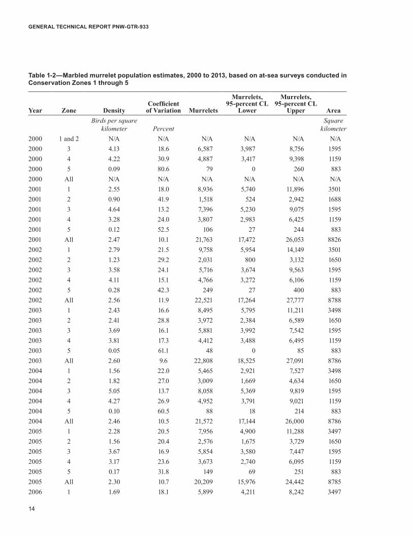
ResultsPopulation EstimatesEstimates of density and population size by conservation zone and for all conservation zones are presented by year in table 1-2. Among conservation zones, murrelet density varied greatly, from less than 0.1 murrelets per square kilometer in Conservation Zone 5 to greater than 5 murrelets per square kilometer in Conservation Zone 4 (table 1-2). Based on these densities, our most recent (2013) population size estimates at the conservation zone scale ranged from about 71 murrelets in Conservation Zone 5 to 7,880 murrelets in Conservation Zone 3 (table 1-2). Conservation Zones 1 and 3 had the two highest population estimates in all years except 2008 and 2013, when Conservation Zones 3 and 4 had the highest estimates (table 1-2). Conservation Zone 5 supported far fewer murrelets than any other conservation zone, with population estimates never exceeding 300 murrelets.
Because population estimates are the product of both density and area of coastal waters sampled, density patterns at the conservation zone scale did not closely
14
GENERAL TECHNICAL REPORT PNW-GTR-933
Table 1-2—Marbled murrelet population estimates, 2000 to 2013, based on at-sea surveys conducted in Conservation Zones 1 through 5
Year Zone Density Coefficient
of Variation Murrelets
Murrelets, 95-percent CL
Lower
Murrelets, 95-percent CL
Upper AreaBirds per square
kilometer PercentSquare
kilometer2000 1 and 2 N/A N/A N/A N/A N/A N/A2000 3 4.13 18.6 6,587 3,987 8,756 15952000 4 4.22 30.9 4,887 3,417 9,398 11592000 5 0.09 80.6 79 0 260 8832000 All N/A N/A N/A N/A N/A N/A2001 1 2.55 18.0 8,936 5,740 11,896 35012001 2 0.90 41.9 1,518 524 2,942 16882001 3 4.64 13.2 7,396 5,230 9,075 15952001 4 3.28 24.0 3,807 2,983 6,425 11592001 5 0.12 52.5 106 27 244 8832001 All 2.47 10.1 21,763 17,472 26,053 88262002 1 2.79 21.5 9,758 5,954 14,149 35012002 2 1.23 29.2 2,031 800 3,132 16502002 3 3.58 24.1 5,716 3,674 9,563 15952002 4 4.11 15.1 4,766 3,272 6,106 11592002 5 0.28 42.3 249 27 400 8832002 All 2.56 11.9 22,521 17,264 27,777 87882003 1 2.43 16.6 8,495 5,795 11,211 34982003 2 2.41 28.8 3,972 2,384 6,589 16502003 3 3.69 16.1 5,881 3,992 7,542 15952003 4 3.81 17.3 4,412 3,488 6,495 11592003 5 0.05 61.1 48 0 85 8832003 All 2.60 9.6 22,808 18,525 27,091 87862004 1 1.56 22.0 5,465 2,921 7,527 34982004 2 1.82 27.0 3,009 1,669 4,634 16502004 3 5.05 13.7 8,058 5,369 9,819 15952004 4 4.27 26.9 4,952 3,791 9,021 11592004 5 0.10 60.5 88 18 214 8832004 All 2.46 10.5 21,572 17,144 26,000 87862005 1 2.28 20.5 7,956 4,900 11,288 34972005 2 1.56 20.4 2,576 1,675 3,729 16502005 3 3.67 16.9 5,854 3,580 7,447 15952005 4 3.17 23.6 3,673 2,740 6,095 11592005 5 0.17 31.8 149 69 251 8832005 All 2.30 10.7 20,209 15,976 24,442 87852006 1 1.69 18.1 5,899 4,211 8,242 3497
15
Status and Trend of Marbled Murrelet Populations and Nesting Habitat
Year Zone Density Coefficient
of Variation Murrelets
Murrelets, 95-percent CL
Lower
Murrelets, 95-percent CL
Upper AreaBirds per square
kilometer PercentSquare
kilometer2006 2 1.44 18.0 2,381 1,702 3,433 16502006 3 3.73 12.7 5,953 4,546 7,617 15952006 4 3.41 14.9 3,953 3,164 5,525 11592006 5 0.10 32.8 89 35 150 8832006 All 2.08 8.2 18,275 15,336 21,214 87852007 1 2.00 24.2 6,985 4,148 10,639 34972007 2 1.54 26.7 2,535 1,318 3,867 16502007 3 2.52 19.8 4,018 2,730 5,782 15952007 4 3.23 34.8 3,749 2,659 7,400 11592007 5 0.03 37.7 30 0 49 8832007 All 1.97 13.7 17,317 12,654 21,980 87852008 1 1.34 17.6 4,699 3,000 6,314 34972008 2 1.17 22.1 1,929 1,164 2,868 16502008 3 3.86 14.7 6,153 4,485 8,066 15952008 4 4.56 17.9 5,285 3,809 7,503 11592008 5 0.08 48.1 67 9 132 8832008 All 2.06 8.9 18,134 14,983 21,284 87852009 1 1.61 21.2 5,623 3,786 8,497 34972009 2 0.77 21.9 1,263 776 1,874 16502009 3 3.70 17.7 5,896 3,898 7,794 15952009 4 3.79 19.9 4,388 3,599 6,952 11592009 5 0.10 50.6 90 11 186 8832009 All 1.96 10.6 17,260 13,670 20,851 87852010 1 1.26 20.0 4,393 2,719 6,207 34972010 2 0.78 25.5 1,286 688 1,961 16502010 3 4.50 16.7 7,184 4,453 9,425 15952010 4 3.16 28.5 3,665 2,248 6,309 11592010 5 0.13 52.1 114 13 241 8832010 All 1.89 11.1 16,641 13,015 20,268 87852011 1 2.06 17.4 7,187 4,807 9,595 34972011 2 0.72 33.4 1,189 571 2,106 16502011 3 4.66 16.3 7,436 5,067 9,746 15952011 4 5.20 34.9 6,023 2,782 10,263 11592011 5 0.16 53.0 137 16 295 8832011 All 2.50 12.6 21,972 16,566 27,378 87852012 1 2.41 20.7 8,442 5,090 12,006 3497
Table 1-2—Marbled murrelet population estimates, 2000 to 2013, based on at-sea surveys conducted in Conservation Zones 1 through 5 (continued)
16
GENERAL TECHNICAL REPORT PNW-GTR-933
track population estimates across conservation zones. For example, although Conservation Zone 3 had the largest sin-gle-conservation zone estimate of population size in 2013, murrelet density was slightly higher in Conservation Zone 4, which has a sample area that is 30 percent smaller than Conservation Zone 3. Sample area size also contributes to the high murrelet numbers in Conservation Zone 1, which encompasses an area of sampled coastal waters (about 3500 km2) more than double that of the next largest conservation zone (about 1650 km2, Conservation Zone 2).
At the All-Zones scale, the mean murrelet density ranged from 1.89 per square kilometer (2010) to 2.56 murrelets per square kilometer (2002; table 1-2). Population estimates at this scale varied from 16,600 in 2010 to 22,800 in 2003 (table 1-2; fig. 1-3). From 2011 through 2013, the All-Zones population estimates were higher than observed since 2005. These higher estimates reflect higher population estimates in Conservation Zone 1 in 2011–2012, in addition to high Conservation Zones 3 and 4 estimates in 2011 and 2013 (table 1-2).
At the scale of individual states, average density was markedly higher off the coast of Oregon, where density was about four murrelets per square kilometer in most
years, compared to densities about half this in Washington and California (table 1-3). California supported fewer than half the number of murrelets estimated for the other two states (table 1-3); this does not include the small, isolated population in central California (Henry et al. 2012), which is outside of the area monitored under the NWFP. Popu-lation sizes for both Oregon and Washington were fairly similar (table 1-3), but were more variable among years in Washington (Oregon mean: 7,874 murrelets, coefficient of variation: 13.8 percent; Washington mean: 8,798, coeffi-cient of variation: 24.9 percent).
At a finer scale, the average density over the years of this study varied among PSUs. Some of the observed variation mirrored general density patterns among conser-vation zones, such that all 15 PSUs in Conservation Zone 5 had low average density. Elsewhere, average density among PSUs within a given stratum or conservation zone displayed variation by as much as 10 times or even more in some cases (fig. 1-4).
Note that estimates at the stratum scale, with the distance estimation parameters f(0), E(s), and truncation distance are presented in appendix 3.
Year Zone Density Coefficient
of Variation Murrelets
Murrelets, 95-percent CL
Lower
Murrelets, 95-percent CL
Upper AreaBirds per square
kilometer PercentSquare
kilometer2012 2 0.72 33.5 1,186 564 2,360 16502012 3 3.99 15.5 6,359 4,136 8,058 15952012 4 4.28 24.9 4,960 3,414 8,011 11592012 5 0.12 50.4 104 10 206 8832012 All 2.40 11.4 21,052 16,369 25,736 87852013 1 1.26 27.9 4,395 2,298 6,954 34972013 2 0.77 18.5 1,271 950 1,858 16502013 3 4.94 16.3 7,880 5,450 10,361 15952013 4 5.22 20.5 6,046 4,531 9,282 11592013 5 0.08 45.4 71 5 118 8832013 All 2.24 11.1 19,662 15,398 23,927 8785CL = confidence limits. N/A = not applicable
Table 1-2—Marbled murrelet population estimates, 2000 to 2013, based on at-sea surveys conducted in Conservation Zones 1 through 5 (continued)

17
Status and Trend of Marbled Murrelet Populations and Nesting Habitat
Trend Analyses Population trends—Estimated rates of linear annual change at the scales of the individual conservation zones and State-scale are pre-sented in figures 1-5 and 1-6, where the estimated rate of linear annual change is shown relative to zero (no change) and the overlap of the 95-percent confidence intervals with zero indicates where the evidence is stronger (no or minimal overlap of 0) or not (extensive overlap with 0). In Conservation Zone 1, the data indicate a linear declining trend of 3.9 percent per year (95-percent confidence inter-val: −7.6 to 0). The data also provide strong evidence for a linear decline in Conservation Zone 2 (6.7-percent decline per year; 95-percent confidence interval: −11.4 to −1.8) (table 1-4; figs. 1-5 and 1-7a). Assuming a constant rate of decline, these rates would translate to cumulative popula-
tion declines over a 10-year period of about 33 percent in Conservation Zone 1 and 50 percent in Conservation Zone 2, based on an exponential model of population change (table 1-4). We found no evidence of linear trends in Conservation Zones 3 and 5. In Conservation Zone 4, no trend was detected, but the evidence was not conclusive; the trend estimate was above zero, and the confidence interval for the estimate overlapped zero (1.5 percent per year, 95 percent confidence interval: −0.9 to 4.0) (fig. 1-5, table 1-4).
No trend was detected for the combined “all-zones” five-conservation-zone-area for the 2001–2013 period. Although the trend estimate was below zero, the evidence was not conclusive because the estimate’s 95-percent confidence interval overlapped zero (−1.2 percent per year; 95-percent confidence interval: −2.9 to 0.5) (fig. 1-5; table 1-4).
10,000
15,000
20,000
25,000
30,000
2001 2003 2005 2007 2009 20112002 2004 2006 2008 2010 2012 2013
Num
ber o
f mur
rele
ts
Year
Figure 1-3—Annual marbled murrelet population estimates and 95-percent confidence intervals, for Conservation Zones 1 through 5 combined.
18
GENERAL TECHNICAL REPORT PNW-GTR-933
Table 1-3—Summary of 2000 to 2003 marbled murrelet density and population size estimates at the state scale
Year State Density MurreletsMurrelets, 95-percent
CL LowerMurrelets, 95-percent
CL Upper AreaBirds per square
kilometer Square kilometer2001 Washington 2.01 10,453 7,057 13,849 5,1882002 Washington 2.29 11,789 7,507 16,071 5,1512003 Washington 2.42 12,467 8,906 16,028 5,1492004 Washington 1.65 8,474 5,625 11,322 5,1492005 Washington 2.05 10,533 7,179 13,887 5,1482006 Washington 1.61 8,280 6,024 10,536 5,1482007 Washington 1.85 9,520 5,946 13,095 5,1482008 Washington 1.29 6,628 4,808 8,448 5,1482009 Washington 1.34 6,886 4,486 9,285 5,1482010 Washington 1.10 5,679 3,840 7,518 5,1482011 Washington 1.63 8,376 5,802 10,950 5,1482012 Washington 1.87 9,629 6,116 13,142 5,1482013 Washington 1.10 5,665 3,217 8,114 5,1482000 Oregon 3.85 7,983 4,992 10,974 2,0712001 Oregon 4.43 9,168 6,536 11,800 2,0712002 Oregon 3.64 7,530 4,727 10,333 2,0712003 Oregon 3.56 7,380 5,370 9,390 2,0752004 Oregon 4.40 9,112 6,833 11,391 2,0712005 Oregon 3.36 6,966 4,812 9,120 2,0712006 Oregon 3.68 7,617 5,916 9,318 2,0712007 Oregon 2.59 5,357 3,333 7,381 2,0712008 Oregon 3.64 7,541 5,682 9,400 2,0712009 Oregon 3.58 7,423 5,208 9,638 2,0712010 Oregon 3.95 8,182 5,743 10,621 2,0712011 Oregon 4.05 8,379 5,943 10,815 2,0712012 Oregon 3.76 7,780 5,604 9,956 2,0712013 Oregon 4.74 9,819 7,195 12,443 2,0712000 California 2.28 3,571 2,556 4,585 1,5662001 California 1.31 2,051 1,030 3,073 1,5662002 California 2.04 3,202 2,425 3,980 1,5662003 California 1.90 2,985 2,392 3,579 1,5692004 California 2.55 3,986 3,009 4,964 1,5662005 California 1.73 2,710 2,106 3,313 1,5662006 California 1.52 2,378 1,781 2,976 1,5662007 California 1.56 2,440 1,709 3,170 1,5662008 California 2.53 3,964 3,414 4,515 1,5662009 California 1.88 2,952 2,148 3,755 1,5662010 California 1.72 2,691 1,959 3,424 1,5662011 California 3.33 5,217 4,155 6,279 1,5662012 California 2.22 3,481 2,795 4,167 1,5662013 California 2.67 4,178 3,561 4,795 1,566
CL = confidence limits
19
Status and Trend of Marbled Murrelet Populations and Nesting Habitat
!
!
!
!
!
!
!
!
!
!
!
!
!
!
!
!
!
!
!
!
!
!
!
!
!
!!
!
!
!!
!
!
!
!
!
!
!
!
!!
!
!
!
!
!
!
!
!
!
!
!
!
!
!
!
!
!
!
!
!
!
!
!
!
CANADA
LakeCrescent
GraysHarbor
WillapaBay
Columbia R.
PacificOcean
Strait of Juan de Fuca
Z2
LakeOzette
Strait of Georgia
Puget
Hood
Can
al
Sound
Z1
Z3
LEWIS
CLALLAM
JEFFERSON
KINGMASON
PIERCE
GRAYSHARBOR
PACIFIC
COWLITZ
WHATCOM
SKAGIT
THURSTON
KITSAP
SNOH.
ISLAND
WAHKIAKUM
SANJUAN
Tacoma
Sequim
Astoria
Olympia
Sea-Tac
Seattle
EverettLa Push
Aberdeen
Quilcene
Kalaloch
Neah Bay
Bremerton
Anacortes
Long Beach
Oak Harbor
Bellingham
ClallamBay
PortAngeles
Copalis Beach
Pacific Beach
PortTownsend
oPrimary sampling unit (PSU)
!
!
!
!
!
!
!
!
!
!
!
!
!
!
!
!
!
!
!
!
!
!
!
!
!
!
Z4
LincolnCity
Reedsport
PacificOcean
Z2
Newport
Seaside
Astoria
Coos Bay
Florence
Waldport
Tillamook
LANE
DOUGLAS
COOS
LINCOLN
TILLAMOOK
CLATSOP
!
!
!
!
!
!
!
!
!
!
!
!
!
!
!
!
!
!
!
!
!
!
!
!
!
!
!
!
!
!
!
!
!
CA
Z3
Z5
PacificOcean
DELNORTE
HUMBOLDT
MEND.
OR
Bandon
CoosBay
Brookings
GoldBeach
PortOrford
COOS
CURRY
JOS.
Orick
Eureka
Arcata
Petrolia
Trinidad
CrescentCity
!
!
!
!
!
!
!
!
!
!
!
!
!
!
!
!
!
!
!
!
!
!
!
Z4!
ShelterCove
PacificOcean
!
Ukiah
Rockport
Mendocino
BodegaBay
SantaRosa
Fort Bragg
PointArena
San Francisco
TRINITY
TEHAMA
HUMBOLDT
MENDOCINO
LAKE
GLENN
SONOMA NAPA
COLUSA
MARIN
Average density (birds/km2)
Zones 1 & 2
0 250 25
0 150 15
Km
Mi
Km
Mi
0 25
0 15
Km
Mi
Km
Mi
0 25
0 15
!
!
!
!
!
Zone 3Zone 4
Zone 5
<11–33–5
5–10>10
At the scale of the three states (fig. 1-6; table 1-4), the murrelet population in Washington experienced an estimated average annual rate of decline of −4.6 percent (95-percent confidence interval: −7.5 to −1.5), with the data providing strong evidence for a declining linear trend for the 2001 to 2013 period (fig. 1-6). There was no evidence for a popula-tion decline or increase in Oregon (+0.3 percent per year; 95-percent confidence interval: −1.8 to 2.5). For California, no trend was detected; although the trend estimate was posi-tive, the evidence for a trend was not conclusive because the 95-percent confidence interval overlapped zero (+2.5 percent per year; 95-percent confidence interval: −1.1 to 6.2).
Effects of sea conditions on density and trend estimates—The no-covariate model had the smallest AICc value for 61 percent of the 51 conservation zone-year combinations pro-vided by our analysis. The covariate model (with Beaufort sea state) had the smallest AICc value in the remaining 39 percent (n = 20 cases). Of these covariate models with lower AICc values, the difference in AICc values between the Beaufort and no-covariate model was less than 4.0 in 9 of the 20 cases, suggesting that both models were competitive in these cases.
Although the AICc values do not support a consistent best single approach to be applied to all conservation zones
Figure 1-4—Average marbled murrelet densities at sea by PSU for each conservation zone. Based on mean densities from 2000 to 2013 monitoring data (2001 to 2013 data for Conservation Zones 1 and 2).
20
GENERAL TECHNICAL REPORT PNW-GTR-933
-15
-10
-5
0
5
10
All 1 2 3 4 5
Ann
ual c
hang
e (p
erce
nt)
Zone
Figure 1-5—Trend results: average rate of annual change by conservation zone and for all conservation zones combined, 2000 to 2013, with 95-percent confidence intervals. The All Zones, Conservation Zone 1, and Conser-vation Zone 2 trends are based on 2001 to 2013 data.
Table 1-4—Estimates of average annual rate of population change and cumulative population change for each conservation zone, for “All Zones” combined, and for each state
Conservation zoneAnnual rate
of change
95-percent confidencelimits Cumulative
change over 10 years Adjusted R2 P-valueLower Upper
Percent PercentAll zones −1.2 −2.9 0.5 −11.3 0.099 0.1561 −3.9 −7.6 0.0 −32.8 0.244 0.0502 −6.7 −11.4 −1.8 −50.0 0.396 0.0133 0.6 −2.1 3.3 +6.2 0 0.6434 1.5 −0.9 4.0 +16.1 0.064 0.1955 −1.0 −8.3 6.9 −9.6 0 0.785Washington −4.6 −7.5 −1.5 −37.6 0.449 0.007Oregon 0.3 −1.8 2.5 +3.0 0 0.756California 2.5 −1.1 6.2 +28.0 0.092 0.154Note that we used data from 2001–2013 for the Washington and Conservation Zones 1 and 2 estimates, and for all others we used data from 2000 to 2013. All trends assume a constant (linear) annual rate of change; see text for details.
21
Status and Trend of Marbled Murrelet Populations and Nesting Habitat
and years, the resulting Beaufort and no-covariate density estimates do not show large differences relative to the standard errors for the density estimates (fig. 1-8).
Based on the results of this analysis, we are continuing the method of using “no-covariate” models to estimate murrelet population density and trends throughout this report, but will evaluate alternatives for future analyses. One such alternative would be to make a separate decision on which model to use for every year and conservation zone combination, based on AICc values.
Power to detect trends—One measure for assessing the effectiveness of the monitor-ing design is its power to detect linear trends in the density (and the correlated population size) of murrelets over time. Detailed results are provided in appendix 1, in which tables A-1 and A-2 present the estimated calendar year when sam-
pling will have been sufficient to detect a population trend for two levels of power. These power numbers measure the ability of the sampling design to detect a trend of a specified magnitude or greater, and are presented for a range of rates of annual decrease. This power analysis is based on annual density estimates through 2013, and forecasts the program’s ability to detect trends under a reduced sampling effort beginning in 2014.
For a given level of power, fewer years of sampling are required to detect a larger decline than a smaller decline. For example, the power analysis indicates that sampling through 2013 has already been sufficient to test for a 5-percent decline with 80 percent power in three of five conservation zones. In comparison, for every zone, and with a sampling frequency of every other year, sampling would need to continue through 2020 (Conservation Zone 3) or later to test for a 2-percent decline with 80-percent power. The power to detect a given trend varies among zones, and one factor influencing power appears to be murrelet density. The number of years required to detect a decline was inversely related to average density for a conservation zone (fig. 1-9) (linear regression R2 = 0.79, P = 0.04, for detecting a 2-percent decline with 80-percent power, n = 5). This is consistent with the general pattern of greater variability for estimates at smaller spatial scales (standard error for single conservation zone versus for all conservation zones combined), and for conservation zones with lower density (table 1-2). For example, Conservation Zone 5 supports the lowest murrelet density of the five conservation zones, and requires the largest number of years to achieve a given level of statistical power (tables A-1 and A-2).
Temporal and spatial variation in marbled murrelet dis-tribution as a function of distance from shore—To minimize the variance in our overall murrelet density estimate, we devoted more sampling effort in the near-shore region where, based on preliminary data, murrelet density was higher (Bentivoglio et al. 2002, Raphael et al. 2007). Comparing density ratios in fig. 1-10, we see that our assumption of greater nearshore density is supported in nearly all year/strata/zone combinations. The ratios shown represent 108 unique zone-stratum-year
8
6
4
2
0
-2
-4
-6
-8
-10Washington Oregon California
Ann
ual c
hang
e (p
erce
nt)
Zone
Figure 1-6—Trend results: average rate of annual change by state, 2000 to 2013, with 95-percent confidence intervals. Washington trend is based on 2001 to 2013 data.
22
GENERAL TECHNICAL REPORT PNW-GTR-933
2000
2002
2004
2006
2008
2010
2012
0123456Zo
ne 1
Year
2000
2002
2004
2006
2008
2010
2012
0123456Zo
ne 4
Year
2000
2002
2004
2006
2008
2010
2012
0123456
Year
Zone
2
2000
2002
2004
2006
2008
2010
2012
0123456
Year
Zone
5
2000
2002
2004
2006
2008
2010
2012
0123456
Year
Zone
3
2000
2002
2004
2006
2008
2010
2012
0123456
Year
All
zone
s co
mbi
ned
Density (birds/km2) Density (birds/km2)
Density (birds/km2) Density (birds/km2)
Density (birds/km2) Density (birds/km2)
2000
2002
2004
2006
2008
2010
2012
0123456
Year
Density (birds/km2)
Ore
gon
2000
2002
2004
2006
2008
2010
2012
0123456
Year
Density (birds/km2)
Cal
iforn
ia
2000
2002
2004
2006
2008
2010
2012
0123456W
ashi
ngto
n
Year
Density (birds/km2)
Figu
re 1
-7—
(A) R
esul
ts o
f tre
nd a
naly
ses a
t All
Zone
s and
indi
vidu
al c
onse
rvat
ion
zone
scal
es. G
raph
s sho
w fi
tted
regr
essi
on li
nes t
hrou
gh th
e an
nual
pop
ulat
ion
estim
ates
for t
he p
erio
d of
ana
lysi
s, w
ith 9
5-pe
rcen
t con
fiden
ce in
terv
als.
(B) R
esul
ts o
f tre
nd a
naly
ses a
t the
stat
e sc
ale.
Gra
phs s
how
fitte
d re
gres
sion
line
s thr
ough
th
e an
nual
pop
ulat
ion
estim
ates
for t
he p
erio
d of
ana
lysi
s, w
ith 9
5-pe
rcen
t con
fiden
ce in
terv
als.
A B
23
Status and Trend of Marbled Murrelet Populations and Nesting Habitat
No
cova
riate
sB
eauf
ort
0.35
0.30
0.25
0.20
0.15
0.10
0.05
020
0020
0220
0420
0620
0820
1020
12
1 023456Zo
ne 3
Year
Density (birds/km2)
2000
2002
2004
2006
2008
2010
2012
1 0234567
Year
Zone
4
2000
2002
2004
2006
2008
2010
2012
Year
Zone
5
2000
2002
2004
2006
2008
2010
2012
Year
2000
2002
2004
2006
2008
2010
2012
Year
Zone
2Zo
ne 1
0.30
0.25
0.20
0.15
0.10
0.05
0
0.35
0.30
0.25
0.20
0.15
0.10
0.05
0
Density (birds/km2)
Figu
re 1
-8—
Effe
ct o
f sea
con
ditio
n (B
eauf
ort)
cova
riate
on
annu
al d
ensi
ty e
stim
ates
at t
he c
onse
rvat
ion
zone
scal
e.
24
GENERAL TECHNICAL REPORT PNW-GTR-933
combinations, of which only 4 are clearly below 1.0 and two are approximately 1.0; the mean ratio at the stratum scale (averaged over all strata and years) is 8.3. In other words, in only 4 percent of the cases did we observe a higher density in the offshore subunit. Even in Stratum 2 of Conservation Zone 2, where most of these low ratios are observed, the ratio is above 1.0 or ≈1.0 for the majority (10 of 13) of years. In addition, this particular strata has very low densities of murrelets and consequently has little influence on the precision of the rangewide population estimates and trend.
In figure 1-10, we present the inshore-to-offshore murrelet density ratio for each year-conservation zone-stra-tum combination. When examining these ratios for all eight conservation zone-strata combinations in fig. 1-10, we see no pattern to these ratios over time in most conservation zones. In Conservation Zone 4, there is some evidence for a declining ratio between 2003 and 2013 for both strata, but this pattern breaks down for the full time series (linear regression, Stratum 1: R2 = 0.16, P = 0.15; Stratum 2: R2 = 0.09, P = 0.29).
DiscussionThis report provides the third evaluation of murrelet population status and trends, following previous reports associated with 10 years (Miller et al. 2006) and 15 years (Davis et al. 2011, Miller et al. 2012) of NWFP implementation. The new analyses reported here indicate that marbled murrelet population numbers vary over space and time throughout the NWFP area, and evaluation at a finer scale than the NWFP area is informa-tive for conservation purposes. Such variation is not surprising given that the factors affecting murrelet density and trend are expected to differ across the NWFP area, which encompasses about 11 degrees of latitude. Previously, the number of years in our sample size limited our ability (statistical power) to test for population trends at the conservation-zone scale, thus limiting our interpretations to the NWFP-wide scale.
At the conservation-zone scale, as observed in previous reports, murrelet density and abundance varied widely among conservation zones, with the most recent (2013) population estimates ranging from about 71 murrelets in Conservation Zone 5 to 7,880 murrelets in Conservation Zone 3. Differences among conservation zone population estimates are a result of variation of both murrelet density and the area of marine
12
34
5
12
43
5
0
10
20
30
40
50
60
0 1 2 3 4 5
Year
s to
det
ect t
rend
Density
80 percent power, 2 percent decline95 percent power, 4 percent decline
Figure 1-9—The number of years of sampling (starting in 2000 or 2001) needed to detect a declining trend at the conservation zone scale as a function of mean conservation zone density, averaged over 2001 to 2013. Each point represents a conservation zone, with points labeled with corresponding conservation zones.
25
Status and Trend of Marbled Murrelet Populations and Nesting Habitat
5
10
15
20
25Zone 1 Stratum 1
Insh
ore:
Offs
hore
ratio
Insh
ore:
Offs
hore
ratio
Insh
ore:
Offs
hore
ratio
Insh
ore:
Offs
hore
ratio
2002 2004 2006 2008 2010 2012
2
3
4
5
6
Zone 1 Stratum 2
Year2002 2004 2006 2008 2010 2012
Year
2002 2004 2006 2008 2010 2012Year
2002 2004 2006 2008 2010 2012Year
2002 2004 2006 2008 2010 2012Year
2002 2004 2006 2008 2010 2012Year
2002 2004 2006 2008 2010 2012Year
2002
20002000
20002000 2004 2006 2008 2010 2012Year
1.0
1.5
2.0
2.5
3.0Zone 2 Stratum 1
0123456
Zone 2 Stratum 2
5
10
15
20
25Zone 3 Stratum 1
102030405060
Zone 3 Stratum 2
Insh
ore:
Offs
hore
ratio
Insh
ore:
Offs
hore
ratio
Insh
ore:
Offs
hore
ratio
5
10
15
Zone 4 Stratum 1
5
10
15
Zone 4 Stratum 2
Rat
io o
f nea
rsho
re to
fars
Figure 1-10—Temporal pattern of marbled murrelet density at stratum scale with respect to the ratio of murrelet density in the inshore versus offshore sampling units. See text for details.

26
GENERAL TECHNICAL REPORT PNW-GTR-933
coastal waters being sampled. The density estimates ranged from 0.1 murrelets per square kilometer in Conservation Zone 5 to 5.2 murrelets per square kilometer in Conservation Zone 4. The target population for Conservation Zone 1 inhabits an area of marine waters double that of any other zone, owing to the large area of marine waters associated with the complex shorelines of the Puget Sound and the San Juan Islands. Annual population estimates for the entire NWFP area ranged from about 16,600 to 22,700 murrelets during the 14-year period, and included the lowest population estimate to date, for 2010.
At the 10-year interval, which followed the first 4 years of monitoring for the Northwest Forest Plan, we did not detect a decline in murrelet densities (Miller et al. 2006). At the 15-year interval, which included monitoring results from 2001 through 2010, we estimated a decline of about 3.7 percent per year at the spatial scale of the five conservation zones combined (Miller et al. 2012). With the addition of estimates through 2013, the evidence for a trend is no longer conclusive at this scale.
With more years of data, the murrelet monitoring program had greater power to evaluate for trends at the scale of the five conservation zones. At that scale, we now observe strong evidence of linear population declines in Conservation Zones 1 and 2, and no trend in Conservation Zones 3 and 5. In Conservation Zone 4, which includes southern Oregon and northern California, the trend estimate was positive but with confidence intervals for the estimate overlapping zero, the evidence for a trend was not conclu-sive, and we concluded that no trend was detected for the 2000 to 2013 period.
For the first time, we evaluated for trends in the annual population estimates at the state scale (table 1-3; fig. 1-6), We found strong evidence of an annual 4 to 5 percent linear decline in Washington (P < 0.01). No evidence of a linear trend was found for the murrelet in Oregon. In California, as for Conservation Zone 4, no trend was detected; although the trend estimates were positive, the evidence for a trend was not con-clusive based on the magnitude of the annual rate estimate and the overlap of the confidence intervals with zero (representing no change). It is worth noting that for both Conservation Zone 4 and California, if the pattern of population estimates continues into the future, an increasing trend may be detectable.
With more years of data, we have found that population estimates can vary markedly between years, particularly at the conservation zone scale, with annual estimates being above or below the average trend line. This variability, combined with reduced future sampling effort, contributes to the relatively large number of years of sampling required to confidently test for lower rates of change at the conservation zone scale.
Trend PatternIn Washington there is strong evidence for a declining trend in both Conservation Zones 1 and 2. In northern and central Oregon, as well as at the Oregon state level, we observed no evidence for a trend. In California (Conservation Zone 5 plus the California portion of Conservation Zone 4), the evidence for a trend was not conclusive, but the trend estimate was posi-tive. For the entire Conservation Zone 4, which spans northern California and southern Oregon, the trend analysis indicated a nonsignificant positive slope. These trend results are suggestive of north-south trend pattern, with clear declines to the north, relatively stable populations in the middle (Oregon) and stable populations to the south in California, but with trend estimate values greater than zero. Results of an analysis of factors contributing to variability in murrelet distribution and trends are presented and discussed in chapter 3. Further analysis of the factors contributing to variability in murrelet distribution and population trends is merited, but the results to date suggest that habitat loss is likely contributing to the trend pattern.
One analytic approach for distinguishing factors that contribute to population trends, and which we plan to pursue in future trend analyses, is the use of state-space models (Humbert et al. 2009, Kery and Schaub 2012). These models have the potential to better separate year-to-year variation that results from sampling (observation) error from variation resulting from biological processes, such as a population trend or environmental variability. State-space models generally require more years of data than the linear regression method we have used to date, but the monitoring program’s sample size should soon be sufficient to merit use of these models (P. Lukacs, pers. comm; E. Ward, pers comm).
The magnitude and strength of evidence for a NWFP-wide decline have decreased relative to our
27
Status and Trend of Marbled Murrelet Populations and Nesting Habitat
previous assessments. This difference may be driven by a variety of factors, most notable being the higher population estimates for 2011 and 2012, specifically in Conservation Zone 1, and especially in Stratum 1 of that conservation zone (Strait of Juan de Fuca). In 2011, estimates of murrelet population size increased in all conservation zones except Conservation Zone 2, compared to estimates from previous years. For Con-servation Zone 1, magnitude of increase in 2011 was such that the 95-percent confidence intervals for the 2010 and 2011 estimates do not overlap each other. In 2012, the All-Zones estimate remained higher, as did the Zone 1 estimate (fig. 1-7a; table 1-2; app. 3). In 2013, the All-Zones population estimate was lower than in 2011 or 2012 and the population estimate in Conservation Zone 1 declined from the 2011–2012 levels, while the Conserva-tion Zone 4 estimate was the highest in 14 years, and the Conservation Zone 3 estimate was the second highest (table 1-2). The reasons for the pattern observed in 2011 to 2013 in Conservation Zones 1 and 4 are unknown, but we discuss some potential causes below.
Sampling and Interpretation ChallengesThe challenges of accurately sampling such a mobile and patchily distributed species, and associated uncertainty in density estimates, could have contributed to the increased estimates in recent years, as could other factors. Results of murrelet population monitoring in 2014 and beyond will help clarify population status and trend, as will data explorations underway. For the latter, we have identified several topics to explore:
Has the distribution of marbled murrelets relative to distance from shore changed? Specifically, did mur-relet distribution shift closer to shore in 2011–2013, such that murrelets previously too far offshore to be within our sampling areas moved closer in those years, to put them within the sampled area? We would expect such a shift to be reflected in higher ratios of the inshore-to-offshore density. Our evaluation of this ratio (fig. 1-10) did not find values outside of ratios observed in prior years. The only exception was Conservation Zone 4 Stratum 2 in 2012; however, this is
an area with relatively few murrelets that contributes little to the observed increases for all conservation zones combined.
Do any of the parameters used to estimate density differ in 2011–2012 from previous years? Parameters of interest include the probability density function of detection dis-tances [ f(0) in DISTANCE], the mean number of murrelets per murrelet group detected [E(s) in DISTANCE], and the encounter rate of murrelets during surveys. Data inspection indicates that f(0) and E(s) did not differ markedly in 2011–2013 from prior years in any conservation zone (app. 3), but encounter rates did increase in 2011–2013. Higher encounter rates are consistent with higher murrelet densities, whereas average group size and the density function for detection distances remained similar to other years.
Could the distribution of marbled murrelets within Conservation Zone 1 have shifted from unsampled PSUs to sampled PSUs? Conservation Zone 1 differs from other conservation zones in having only a subset of PSUs sampled each year, with the same PSUs sampled based on an initial random sample in 2000 (Raphael et al. 2007). Changes in density estimates in Stratum 1 of Conservation Zone 1 contributed heavily to the 2011–2012 increases in Conservation Zone 1 estimates. Because not all PSUs are surveyed in this stratum, a movement of murrelets between PSUs could contribute to an increase in estimates. Because we lack data from the unsampled areas, this question is difficult to evaluate.
The removal of two large dams on the Elwha River between 2011 and 2014 generated large sediment plumes within Stratum 1 of Conservation Zone 1 during the survey season, and might also have influenced the distribution and abundance of murrelets in this area. Removal of Elwha Dam began in September 2011, and the final segment of Glines Canyon Dam was removed in August 2014. Conceivably, the sediment input from dam removal could have created a foraging opportunity that attracted murrelets from other PSUs or strata. However, we first observed an increase in murrelet density in Stratum 1 of Conservation Zone 1 in the 2011 survey, months prior to the September 2011 Elwha Dam removal (app. 3).

28
GENERAL TECHNICAL REPORT PNW-GTR-933
Could the distribution of marbled murrelets have shifted from areas outside of Conservation Zone 1 into Conservation Zone 1 during the 2011–2013 period? With respect to movements from south of Conservation Zone 1, our data do not support a systematic shift that would account for the increase during this period (table 1-2; fig. 1-7a). In 2011, the first year of the observed in-crease in Conservation Zone 1, estimates for other con-servation zones were fairly stable (Conservation Zones 2 and 3) or increased (Conservation Zone 4) compared to 2010 (table 1-2), not providing any evidence for movement from the south between 2010 and 2011. In Conservation Zone 2, which is adjacent to Conservation Zone 1, mur-relet densities were very similar from 2009 through 2013. Our murrelet density estimates from Conservation Zone 3 increased or were stable in 2010, 2011, and 2013 com-pared to the several years prior to 2010 (fig. 1-7a), which is not consistent with movement of murrelets from this zone into Conservation Zone 1. Similarly, in Conservation Zone 4, density estimates in 2011 through 2013 were equal or greater than densities in 2009–2010. Numbers of murrelets decreased in 2012 (when Conservation Zone 1 numbers in-creased) in Conservation Zones 3 and 4, compared to 2011 and 2013. Although between-zone movements could have contributed to annual variations observed within this 3-year period, they do not explain the overall increase observed in Conservation Zone 1 during the 2011–2012 period, com-pared to previous years (table 1-2, fig. 1-7a).
Murrelets could have moved from the north into our sample area, such as across the Strait of Juan de Fuca from British Columbia to northern Washington. Comparable regional results are not available from British Columbia. However, available data for evaluating this possibility are limited to a single long-term at-sea sampling effort from about 100 km of transects on the southwest coast of Van-couver Island during May to July. Results from this effort suggest a marked increase in murrelet numbers during the 2001 to 2013 period, especially during the years 2010, 2011, and 2013 compared to previous years (Y. Zharikov, pers. comm.). The data from this small area, which is in part on the Strait of Juan de Fuca, are not consistent with a marked emigration of murrelets out of their study area. It
remains possible that the influx of murrelets in Conserva-tion Zone 1 came from areas even farther north in British Columbia or Alaska.
Were fewer murrelets breeding in 2011 and 2012, re-sulting in more adult murrelets on the water than at nest sites? During the approximate 29-day incubation period and first 1 to 2 days after hatching, one of the mur-relet adults is present on the nest (Nelson 1997), and thus is not available to be counted at-sea. The incubation period (Nelson 1997) closely overlaps our sampling period, thus, if fewer murrelets attempted nesting, we would expect to detect more murrelets on the water. The ratio of hatch-year to after-hatch-year murrelets observed on surveys during the fledging period is one measure of reproductive suc-cess (Peery et al. 2007). This ratio, as well as numbers of hatch-year murrelets counted around the San Juan Islands in 2011–2012 were comparable to or greater than num-bers in other years (Havron 2012), which is not consistent with fewer murrelets nesting for the murrelet population associated with the waters around the San Juan Islands, in Conservation Zone 1. Also, anecdotal observations from the California Current System, which includes west-ern Washington, and peripherally the western portion of Conservation Zone 1, indicate good years for marine pro-ductivity and forage fish during 2011–2013 (Peterson et al. 2013), which would tend to lead to more murrelets nesting (Peery et al. 2004). Indicative of this, in Conservation Zone 3, hatch-year murrelets occurred at near-average densities in 2011 and 2012, and at anomalously high densities in 2013 (Strong 2014). This would not support a lower propor-tion of murrelets breeding, at least within the California Current System.
Potential effects of high rates of nesting success and recruitment,and/orearlyfledging. High rates of nesting success, particularly if combined with earlier fledging than normal, could potentially result in higher densities of hatch-year murrelets. Murrelet fledgling numbers at sea typically peak in late July to August (Nelson 1997), which only slightly overlaps our sampling, which extends from May 15 to July 31. As noted above, marine productivity was good in 2011 to 2013, at least in the California Current System,
29
Status and Trend of Marbled Murrelet Populations and Nesting Habitat
and good ocean productivity and prey quality tend to be associated with greater nesting success and recruitment in marbled murrelets (Becker and Beissinger 2006, Becker et al. 2007, Norris et al. 2007).
Could habitat change have caused the observed pattern? Murrelet nesting habitat takes many decades to several centuries to develop (USFWS 1997), thus is a process too slow to account for the rapid increase in density estimates observed in a period of less than 10 years.
Potential Uncertainties in SamplingWe reviewed several sources of potential bias that could affect our observed trends. For example, we anticipated a seasonal increase in murrelet density during the sampling period as chicks hatched and incubating murrelets returned to the water to forage, making only short flights inland to feed chicks (Peery et al. 2007). However, examination of the data early in the monitoring program (Miller et al. 2006) did not find a temporal trend within a season. This lack of a seasonal trend may be due to a variety of factors, including a small proportion of murrelets breeding in any one year or the early return to the ocean of breeders whose nests failed during incubation. Our objectives in this study were to estimate the average number of murrelets in our target area between May 15 and July 31 and to be able to detect trends in those estimates. Our sampling design, which distributed sampling effort consistently through this period, allows us to meet our objectives even if the number of murrelets on the water during the sampling period was not constant.
More sampling effort was devoted to the inshore subunit, where data from previous work had shown densities to be highest. Based on average densities since 2000, densities in the inshore subunit were typically higher, and on average about eight times higher than in the offshore subunit. Densities were higher in the offshore subunit in only 4 of 108 stratum-year combinations sampled. Three of these year-stratum combinations were clustered in the southern half of Conservation Zone 2, near the Columbia River estuary and plume, as well as being in an area where the continental shelf is broad. Perhaps murrelet distribution in this area extends in
some years further offshore than assumed. Murrelets can occur farther offshore where shallow waters and islets extend farther offshore (Ralph and Miller 1995, Raphael et al. 1999, Speich and Wahl 1995, Strong et al. 1995). If so, it should not influence our trend results for the target population, but could mean that in this stratum the area of coastal waters sampled represents less than the design target of 95 percent of the local population. The effect on our population estimates should be relatively small, as this area has very low densities of murrelets (fig. 1-4). A long-term (multiyear), systematic shift in murrelet distribution toward further offshore could affect our ability to assess population trends if it resulted in a substantial change in the proportion of murrelets occurring beyond the waters sampled. We evaluated the annual density estimates for each conservation zone for evidence of a trend since 2000–2001 of murrelet distribution shifting further off-shore, and found no evidence of such a pattern to date. In the future, we will evaluate whether the data collected by the monitoring program can be used to explicitly evaluate the protocol’s assumption that coastal waters sampled encompass at least 95 percent of the local population during the sample period.
Other studies have found year, observer, and sea-state effects on detectability and at-sea density estimates for murrelets (Ronconi and Burger 2009). These factors, if not accounted for, can potentially increase error in our estimates, and thus reduce the power to detect trends. Our trend analyses explicitly accounted for year effects. We assessed observer (crew) effects in an earlier analysis of Conservation Zone 1 data (Miller et al. 2012) and found no observer effect on density or trend estimates, which may be reflective of our training efforts and low crew turnover. Our analysis of sea-state demonstrated a relatively slight effect on density and trend estimates, and no effect that would change our conclusion about the direction or magnitude of any trend. Sea-state effects are in part reduced by our protocol, which precludes surveys during poor sea condi-tions. Although we did not include a sea-state covariate in the analyses in this report, we will continue to evaluate the influence of sea state on murrelet detection and ultimately on trend estimates.

30
GENERAL TECHNICAL REPORT PNW-GTR-933
Given the goals of the NWFP and the monitoring program, ideally, any population trends we observe through monitoring should reflect changes in nesting habitat conditions within the NWFP area. However, biological systems are rarely closed, particularly when defined by political boundaries. There is likely some movement of murrelets between the northern portion of our sampling area and Canadian waters to the north. Suitable nesting habitat continues north from Washington into British Columbia, both on the mainland and Van-couver Island, and such movements have been observed. In a telemetry study, Raphael and colleagues (Bloxton and Raphael 2009) recorded movements between U.S. waters and nesting sites on nearby Vancouver Island but no long-distance movements consistent with individuals shifting their distribution from Washington to areas north of our study area, or vice-versa. Similarly, a telemetry study in northern California (Hebert and Golightly 2008) found that murrelets traveled less than 50 km away from the mouth of the watershed where most nesting occurred (Hebert and Golightly 2008). However, these studies occurred during the breeding season, when nesting mur-relets would be unlikely to make long shifts in location.
A northward shift of the murrelet’s distribution from Washington into Canada could mimic the decline observed in Conservation Zone 1 (Puget Sound and Strait of Juan de Fuca) and could also affect trends in coastal Washington, Conservation Zone 2. However, we know of no evidence or causal mechanism for such a shift from 2001 to 2013, and the available data indicate that such a shift is unlikely. The murrelet’s distribution at sea during the breeding season generally coincides with the distri-bution of potential nesting habitat directly inland (Burger 2002; Meyer et al. 2002; Miller et al. 2002; Raphael 2006; Raphael et al. 2002, 2015), suggesting that most murrelets observed on the water represent local breeding populations. A large northward population shift would suggest that breeding individuals are shifting nest loca-tions, which is not supported by the limited information on nest-site fidelity. Nest-site fidelity is common in other alcids (Divoky and Horton 1995), and individual marbled murrelets have been observed re-nesting in the same
stands and trees in successive years, suggesting some fidelity to nest areas (Hebert et al. 2003, Piatt et al. 2007). Also, population-trend data from British Columbia from the 1990s to 2006 do not support a shift from Washington waters to British Columbia, where there is some evidence for a decline during this period (Piatt et al. 2007). When examining the previously mentioned yearly monitoring by Zharikov on the southwest coast of Vancouver Island in British Columbia, there is no evidence that murrelets are shifting between Conservation Zone 1 and southwest Vancouver Island during the monitoring period. A recent analysis of British Columbia murrelet population trends during 1996 through 2013, based on a radar-based mon-itoring program, found negative annual trends for two of the three sampling regions adjacent to Washington (East Vancouver Island and South Mainland Coast), and no trend in the third region (West and North Vancouver Island) (Bertram et al. 2015). Finally, Piatt et al. (2007) reported a substantial and continuing loss of likely mur-relet nesting habitat on Vancouver Island and Haida Gwaii since the 1970s.
Potential Causes for DeclineThe NWFP population monitoring reported here does not address the causes of population trends. However, the other chapters in this volume report on companion analyses that provide some insight into potential causes. Chapter 2 documents the loss of murrelet nesting habitat within the area of the NWFP, with the most acres of loss occurring in Washington. Chapter 3 uses the findings from murrelet population and nesting habitat monitoring to explore the relationships between quantity and quality of inland forest, prey availability, ocean conditions, and murrelet densities at sea in the NWFP area, building on a previous analysis (Raphael et al. 2015). As detailed in chapter 3, analysis of those relationships suggests that the amount and spatial pattern of nesting habitat, and changes therein, were the strongest predictors of murrelet numbers and trend in nearby marine waters.
In conclusion, this monitoring program provides pop-ulation information, available nowhere else, on the status of marbled murrelets in the Northwest Forest Plan area,
31
Status and Trend of Marbled Murrelet Populations and Nesting Habitat
as well as being the only population information available to inform the species’ recovery and ultimate delisting. A conservation goal of the NWFP is to stabilize and increase murrelet populations by maintaining and increasing nesting habitat. In this report, we address a primary question for evaluating the plan’s effectiveness in achieving this goal during the first 20 years of NWFP implementation: Is the marbled murrelet population stable or increasing? Our findings indicate that the answer to this question is “no,” the murrelet population associated with the NWFP area is not stable or increasing, at least not in Washington. We believe that the magnitude of the decline observed for Washington state and its two conservation zones, based on the 2001 to 2013 period, is sufficient to cause concern, and may merit a review of potential management implications and responses.
Management implications of results to date from the marbled murrelet effectiveness monitoring program are provided in detail in chapter 3. The trend pattern to date is of concern, particularly for Washington, where the murrelet population has not stabilized. Both the NWFP (FEMAT 1993) and the species’ recovery plan (USFWS 1997) antic-ipated a challenge in maintaining murrelet populations for 50 to 200 years, until new nesting habitat develops. In light of observed population trends, our findings underscore the importance of the short-term goal to maintain existing nesting habitat. Long-term monitoring of murrelet populations and their environment, including nesting habitat, should reveal whether the NWFP meets its conservation goal of stabilizing and ultimately increasing marbled murrelet populations by maintaining and increasing nesting habitat. With long-term monitoring, we may also better understand the mechanisms underlying population change, and the degree to which population changes are linked to nesting habitat conditions on the lands managed under the Northwest Forest Plan.
AcknowledgmentsThis work would not have been possible without the assistance of a large number of people who contributed to the population monitoring program. We particularly thank the many crew members who conducted the at-sea popula-tion surveys over the years, often under difficult conditions. Naomi Bentivoglio, Patrick Jodice, and Mark Huff provided leadership for the marbled murrelet monitoring program in its early years. Former monitoring team members Sherri Miller and C.J. Ralph were instrumental in establishing marbled murrelet at-sea surveys in California and elsewhere, and made many contributions to the program, as did past team members Tom Bloxton and Beth Galleher. Funding and other support for this work was provided by several offices and programs of the U.S. Fish and Wildlife Service, by the U.S. Forest Service Pacific Northwest Research Station and Pacific Northwest Region, the U.S. Forest Service Pacific Southwest Forest Research Station and Pacific Southwest Region, the Bureau of Land Management Arcata Field Office, the Washington State Department of Fish and Wildlife, the California Department of Fish and Wildlife, and the Pacific Lumber Company (now the Humboldt Red-woods Company). We thank Yuri Zharikov of the Pacific Rim National Park Reserve of Canada for sharing results from marbled murrelet surveys off the coast of Vancouver Island. This report benefited from comments by Nathalie Hamel, Mark Huff, and Paul Lukacs, and from numerous discussions with Ray Davis. The findings and conclusions in this article are those of the authors and do not necessarily represent the views of the U.S. Fish and Wildlife Service.
32
GENERAL TECHNICAL REPORT PNW-GTR-933
ReferencesBecker, B.H.; Beissinger, S.R. 2006. Centennial decline in
the trophic level of an endangered seabird after fisheries decline. Conservation Biology. 20: 470–479.
Becker, B.H.; Peery, M.Z.; Beissinger, S.R. 2007. Ocean climate and prey availability affect the trophic level and reproductive success of the marbled murrelet, and endangered seabird. Marine Ecology Progress Series. 329: 267–279.
Bentivoglio, N.; Baldwin, J.; Jodice, P.G.R.; Evans Mack, D.; Max, T.; Miller, S.; Nelson, S.K.; Ostrom, K.; Ralph, C.J.; Raphael, M.; Strong, C.; Thompson, C.; Wilk, R. 2002. Northwest Forest Plan marbled murrelet effectiveness monitoring 2000 annual report. Portland, OR: U.S. Department of the Interior, Fish and Wildlife Service. 72 p. http://www.reo.gov/monitoring/reports/murrelet/MAMU_EM_00report.pdf. (17 June 2015).
Bertram, D.F.; Drever, M.C.; McAllister, M.K.; Schroeder, B.K.; Lindsay, D.J.; Faust, D.A. 2015. Estimation of coast-wide population trends of marbled murrelets in Canada using a Bayesian hierarchical model. PLoS ONE. 10(8):e0134891. doi:10.1371/journal.pone.0134891.
Bloxton, T.D.; Raphael, M.G. 2009. Breeding ecology of the marbled murrelet in Washington State: five year project summary (2004–2008). Unpublished report. On file with: U.S. Department of Agriculture, Forest Service, Pacific Northwest Research Station, Forestry Sciences Laboratory, 3625 93rd Ave., Olympia, WA 98512-9193. 41 p.
Buckland, S.T.; Anderson, D.R.; Burnham, K.P.; Laake, J.L.; Borchers, D.L.; Thomas, L. 2001. Introduction to distance sampling: estimating abundance of biological populations. New York: Oxford University Press. 448 p.
Buckland, S.T.; Anderson, D.R.; Burnham, K.P.; Laake, J.L.; Borchers, D.L.; Thomas, L. 2004. Advanced distance sampling: estimating abundance of biological populations. New York: Oxford University Press. 434 p.
Burger, A.E. 2002. Conservation assessment of marbled murrelets in British Columbia, a review of the biology, populations, habitat associations, and conservation. Technical Report 387. Delta, British Columbia, Canada: Canadian Wildlife Service. 194 p.
Cochran, W.G. 1977. Sampling techniques. 3rd ed. New York: John Wiley and Sons. 428 p.
Davis, R.; Falxa, G.; Grinspoon, E.; Harris, G.; Lanigan, S.H.; Moeur, M.; Mohoric, S. 2011. Northwest Forest Plan—the first 15 years [1994–2008]: Monitoring the Northwest Forest Plan—summary of key findings. Tech. paper R6-RPM-TP-03-2011. Portland, OR: U.S. Department of Agriculture, Forest Service, Pacific Northwest Region. 42 p.
Divoky, G.J.; Horton, M. 1995. Nest habitat loss and implications for marbled murrelet populations. In: Ralph, C.J.; Hunt, G.L.; Raphael, M.G.; Piatt, J.F., eds. Ecology and conservation of the marbled murrelet. Gen. Tech. Rep. PSW-GTR-152. Albany, CA: U.S. Department of Agriculture, Forest Service, Pacific Southwest Research Station: 83–87.
Falxa, G.; Baldwin, J.; Lance, M.; Lynch, D.; Nelson, S.K.; Pearson, S.F.; Raphael, M.G.; Strong, C.; Young, R. 2014. Marbled murrelet effectiveness monitoring, Northwest Forest Plan: 2013 summary report. 20 p. http://www.reo.gov/monitoring/reports/murrelet/MAMU_2013_NWFP%20EM_Annual%20Report_May2014.pdf. (17 June 2015).
Forest Ecosystem Management Assessment Team [FEMAT]. 1993. Forest ecosystem management: an ecological, economic, and social assessment. Portland, OR: U.S. Department of Agriculture; U.S. Department of the Interior; [and others]. [Irregular pagination].
Havron, A. 2012. Summary report of field observations of marbled murrelets in the San Juan Islands, Washington. Unpublished report. On file with: U.S. Department of Agriculture, Forest Service, Pacific Northwest Research Station, Forestry Sciences Laboratory, 3625 93rd Ave., Olympia, WA 98512-9193.

33
Status and Trend of Marbled Murrelet Populations and Nesting Habitat
Hebert, P.N.; Golightly, R.T. 2008. At-sea distribution and movements of nesting and non-nesting marbled murrelets Brachyramphus marmoratus in northern California. Marine Ornithology. 36: 99–105.
Hebert, P.N.; Golightly, R.T.; Orthmeyer, D.L. 2003. Radiotelemetry evidence of renesting in the same season by the marbled murrelet. Waterbirds. 26: 261–265.
Henry, R.W.; Tyler, W.B.; Peery, M.Z. 2012. Abundance and productivity of marbled murrelets off central California during the 2010 and 2011 breeding seasons: final report submitted to the Luckenbach and Command Oil Spill Trustees. 18 p.
Huff, M.H.; Raphael, M.G.; Miller, S.L.; Nelson, S.K.; Baldwin, J., tech coords. 2006. Northwest Forest Plan—the first 10 years (1994–2003): status and trends of populations and nesting habitat for the marbled murrelet. Gen. Tech. Rep. PNW-GTR-650. Portland, OR: U.S. Department of Agriculture, Forest Service, Pacific Northwest Research Station. 149 p. http://www.fs.fed.us/pnw/pubs/pnw_gtr650.pdf. (17 June 2015).
Humbert, J-Y.; Mills, L.S.; Horne, J.S.; Dennis, B. 2009. A better way to estimate population trends. Oikos. 118: 1940–1946.
Johnson, J.B.; Omland, K.S. 2004. Model selection in ecology and evolution. Trends in Ecology and Evolution. 19: 101–108.
Kery, M.; Schaub, M. 2012. Bayesian population analysis using WinBUGS: a hierarchical perspective. Waltham, MA: Academic Press. 534 p.
Lukacs, P.M. 2015. Personal communication. Associate professor, Department of Ecosystem and Conservation Sciences, College of Forestry and Conservation, University of Montana, Missoula, MT 59812. email: [email protected].
Madsen, S.; Evans, D.; Hamer, T.; Henson, P.; Miller, S.; Nelson, S.K.; Roby, D.; Stapanian, M. 1999. Marbled murrelet effectiveness monitoring plan for the Northwest Forest Plan. Gen. Tech. Rep. PNW-GTR-439. Portland, OR, U.S. Department of Agriculture, Forest Service, Pacific Northwest Research Station. 51 p.
McShane, C.; Hamer, T.; Carter, H.; Swartzman, G.; Friesen, V.; Ainley, D.; Tressler, R.; Nelson, K.; Burger, A.; Spear, L.; Mohagen, T.; Martin, R.; Henkel, L.; Prindle, K.; Strong, S.; Keany, J. 2004. Evaluation report for the 5-year status review of the marbled murrelet in Washington, Oregon, and California. Unpublished report on file with: EDAW, Inc. Seattle, Washington. Prepared for the U.S. Fish and Wildlife Service, Region 1. Portland, Oregon.
Meyer, C.B.; Miller, S.L.; Ralph, C.J. 2002. Multi-scale landscape and seascape patterns associated with marbled murrelet areas on the U.S. west coast. Landscape Ecology. 17: 95–115.
Miller, S.L.; Meyer, C.B.; Ralph, C.J. 2002. Land and seascape patterns associated with marbled murrelet abundance offshore. Waterbirds. 25: 100–108.
Miller, S.L.; Ralph, C.J.; Raphael, M.G.; Strong, C.; Thompson, C.W.; Baldwin, J.; Huff, M.H.; Falxa, G.A. 2006. At-sea monitoring of marbled murrelet population status and trend in the Northwest Forest Plan area. In: Huff, M.H.; Raphael, M.G.; Miller, S.L.; Nelson, S.K.; Baldwin, J., tech. coords. Northwest Forest Plan—the first 10 years (1994–2003): status and trends of populations and nesting habitat for the marbled murrelet. Gen. Tech. Rep. PNW-GTR-650. Portland, OR: U.S. Department of Agriculture, Forest Service, Pacific Northwest Research Station: 31–60. Chapter 3.
Miller, S.L.; Raphael, M.G.; Falxa, G.A.; Strong, C.; Baldwin, J.; Bloxton, T.; Galleher, B.M.; Lance, M.; Lynch, D.; Pearson, S.F.; Ralph, C.J.; Young, R.D. 2012. Recent population decline of the marbled murrelet in the Pacific Northwest. Condor. 114: 771–781.
34
GENERAL TECHNICAL REPORT PNW-GTR-933
Morrison, P.H. 1988. Old growth in the Pacific Northwest: a status report. Washington, DC: The Wilderness Society. 61 p.
Mulder, B.S.; Noon, B.R.; Spies, T.A.; Raphael, M.G.; Palmer, C.J.; Olsen, A.R.; Reeves, G.H.; Welsh, H.H. Jr.; 1999. The strategy and design of the effectiveness monitoring program for the Northwest Forest Plan. Gen. Tech. Rep. PNW-GTR-347. Portland, OR: U.S. Department of Agriculture, Forest Service, Pacific Northwest Research Station. 138 p.
Nelson, S.K. 1997. Marbled murrelet (Brachyramphus marmoratus). In: Poole, A.; Gill, F., eds. The birds of North America, No. 276. http://bna.birds.cornell.edu/bna/species/276/articles/introduction. (17 June 2015).
Norheim, R.A. 1996. Is there an answer to mapping old growth? An examination of two projects conducted with remote sensing and GIS. Seattle, WA: University of Washington. 306 p. M.S. thesis.
Norheim, R.A. 1997. Dueling databases: examining the differences between two old growth mapping projects. Presented at 13th international symposium on computer-assisted cartography (Auto-Carto 13). http://purl.oclc.org/net/norheim/oldgrowth/dueling-db.html. (17 June 2015).
Norris, D.R.; Arcese, P.; Preikshot, D.; Bertram, D.F.; Kyser, T.K. 2007. Diet reconstruction and historic population dynamics in a threatened seabird. Journal Applied Ecology. 44: 875–884.
Peery, M.Z.; Becker, B.H.; Beissinger, S.R. 2007. Age ratios as estimators of productivity: testing assumptions on a threatened seabird, the marbled murrelet. Auk. 124: 224–240.
Peery, M.Z.; Beissinger, S.R.; Newman. S.H.; Burkett, E.B.; Williams, T.D. 2004. Applying the declining populations paradigm: diagnosing causes of poor reproduction in the marbled murrelet. Conservation Biology. 18: 1088–1098.
Peterson, W.T.; Morgan, C.A.; Peterson, J.O.; Fisher, J.L.; Burke, B.J.; Fresh, K. 2013. Ocean ecosystem indicators of salmon marine survival in the northern California Current. Unpublished report on file with: Northwest Fisheries Science Center National Marine Fisheries Service, Newport, Oregon. 77 p.
Piatt, J.F.; Kuletz, K.J.; Burger, A.E.; Hatch, S.A.; Friesen, V.L.; Birt, T.P.; Arimitsu, M.L.; Drew, G.S.; Harding, A.M.A.; Bixler, K.S. 2007. Status review of the marbled murrelet (Brachyramphus marmoratus) in Alaska and British Columbia. Open-File Report 2006–1387. Reston, VA: U.S. Department of the Interior, Geological Survey. 258 p.
Ralph, C.J.; Hunt, G.L.; Raphael, M.G.; Piatt, J.F., eds. 1995. Ecology and conservation of the marbled murrelet. Gen. Tech. Rep. PSW-GTR-152. Albany, CA: U.S. Department of Agriculture, Forest Service, Pacific Southwest Research Station. 420 p.
Ralph, C.J.; Miller, S.L. 1995. Offshore population estimates of marbled murrelets in California. In: Ralph, C.J.; Hunt, G.L.; Raphael, M.G.; Piatt, J.F. eds. Ecology and conservation of the marbled murrelet. Gen. Tech. Rep. PSW-GTR-152. Albany, CA: U.S. Department of Agriculture, Forest Service, Pacific Southwest Research Station: 353–360.
Raphael, M.G. 2006. Conservation of the marbled murrelet under the Northwest Forest Plan. Conservation Biology. 20: 297–305.
Raphael, M.G.; Baldwin, J.; Falxa, G.A.; Huff, M.H.; Lance, M.; Miller, S.L.; Pearson, S.F.; Ralph, C.J.; Strong, C.; Thompson, C. 2007. Regional population monitoring of the marbled murrelet: field and analytical methods. Gen. Tech. Rep. PNW-GTR-716. Portland, OR: U.S. Department of Agriculture, Forest Service, Pacific Northwest Research Station. 70 p. http://www.fs.fed.us/pnw/pubs/pnw_gtr716.pdf. (17 June 2015).
35
Status and Trend of Marbled Murrelet Populations and Nesting Habitat
Raphael, M.G.; Evans, D.; Wilk, R. 1999. Sampling marbled murrelets at sea: tests of survey methods and designs. http://www.reo.gov/monitoring/reports/murrelet/pnw_atsea.pdf. (17 June 2015).
Raphael, M.G.; Evans-Mack, D.; Cooper, B.A. 2002. Landscape-scale relationships between abundance of marbled murrelets and distribution of nesting habitat. Condor. 104: 331–342.
Raphael, M.G.; Falxa, G.A.; Dugger, K.M.; Galleher, B.M.; Lynch, D.; Miller, S.L.; Nelson, S.K.; Young, R.D. 2011. Status and trend of nesting habitat for the marbled murrelet under the Northwest Forest Plan. Gen. Tech. Rep. PNW-GTR-848. Portland, OR: U.S. Department of Agriculture, Forest Service, Pacific Northwest Research Station. 52 p.
Raphael, M.G.; Galleher, B.M.; Huff, M.H.; Miller, S.L.; Nelson, S.K.; Young, R.D. 2006. Spatially-explicit estimates of potential nesting habitat for the marbled murrelet. In: Huff, M.H.; Raphael, M.G.; Miller, S.L.; Nelson, S.K.; Baldwin, J., tech. coords. 2006. Northwest Forest Plan—the first 10 years (1994–2003): status and trends of populations and nesting habitat for the marbled murrelet. Gen. Tech. Rep. PNW-GTR-650. Portland, OR: U.S. Department of Agriculture, Forest Service, Pacific Northwest Research Station: 97–146. Chapter 5.
Raphael, M.G,; Shirk, A.J.; Falxa, G.A.; Pearson, S.F. 2015. Habitat associations of marbled murrelets during the nesting season in nearshore waters along the Washington to California coast. Journal of Marine Systems. 146: 17–25.
Ronconi, R.A.; Burger, A.E. 2009. Estimating seabird densities from vessel transects: distance sampling and implications for strip transects. Aquatic Biology. 4: 297–309.
Sokal, R.R.; Rohlf, F.J. 1981. Biometry: the principles and practice of statistics in biological research. 2nd ed. San Francisco, CA: W.H. Freeman and Co. 859 p.
Speich, S.M.; Wahl, T.R. 1995. Marbled murrelet populations of Washington—marine habitat preferences and variability of occurrence. In: Ralph, C.J.; Hunt, G.L.; Raphael, M.G.; Piatt, J.F., eds. Ecology and conservation of the marbled murrelet. Gen. Tech. Rep. PSW-GTR-152. Albany, CA: U.S. Department of Agriculture, Forest Service, Pacific Southwest Research Station: 313–325.
Strong, C.S. 2014. Marbled murrelet monitoring in Oregon and California during 2013. Final Report to the U.S. Fish and Wildlife Service. On file with: Crescent Coastal Research, 7700 Bailey Rd., Crescent City, CA 95531.Portland, OR. Unpublished report. 26 p.
Strong, C.S.; Keitt, B.S.; McIver, W.R.; Palmer, C.J.; Gaffney, I. 1995. Distribution and population estimates of marbled murrelets at sea in Oregon during the summers of 1992 and 1993. In: Ralph, C.J.; Hunt, G.L.; Raphael, M.G.; Piatt, J.F., eds. Ecology and conservation of the marbled murrelet. Gen. Tech. Rep. PSW-GTR-152. Albany, CA: U.S. Department of Agriculture, Forest Service, Pacific Southwest Research Station: 339–353.
Thomas, L.; Buckland, S.T.; Rexstad, E.A.; Laake, J.S.; Strindberg, S.; Hedley, S.L.; Bishop, J.R.B.; Marques, T.A.; Burnham, K.P. 2010. Distance software: design and analysis of distance sampling surveys for estimating population size. Journal of Applied Ecology. 47: 5–14. doi:10.1111/j.1365-2664.2009.01737.x.
U.S. Department of Agriculture, Forest Service; U.S. Department of the Interior, Bureau of Land Management [USDA and USDI]. 1994. Final supplemental environmental impact statement on management of habitat for late-successional and old-growth forest related species within the range of the northern spotted owl. Volumes I-II + Record of Decision.
36
GENERAL TECHNICAL REPORT PNW-GTR-933
U.S. Department of the Interior, Fish and Wildlife Service [USFWS]. 1990. Endangered and threatened wildlife and plants; determination of threatened status for the northern spotted owl. Federal Register. 55: 26114–26194.
U.S. Department of the Interior, Fish and Wildlife Service [USFWS]. 1992. Endangered and threatened wildlife and plants; determination of threatened status for the Washington, Oregon, and California population of the marbled murrelet. Federal Register. 57: 45328–45337.
U.S. Department of the Interior, Fish and Wildlife Service [USFWS]. 1997. Recovery plan for the threatened marbled murrelet (Brachyramphus marmoratus) in Washington, Oregon, and California. Portland, OR. 203 p.
U.S. Department of the Interior, Fish and Wildlife Service [USFWS]. 2009. Marbled murrelet (Brachyramphus marmoratus): 5 year review. Washington Fish and Wildlife Office, Lacey, WA. 108 p.
Ward, E.J. 2015. Personal communication. Statistician (biology), National Oceanographic and Atmospherics Administration—Fisheries, Northwest Fisheries Science Center, 2725 Montlake Blvd. East, Seattle, WA 98112. email: [email protected].
Zharikov, Y. Year. Personal communication, Monitoring Ecologist, Pacific Rim National Park Reserve of Canada, Box 280, Ucluelet, British Columbia, V0R 3A0, Canada. email: [email protected].
37
Status and Trend of Marbled Murrelet Populations and Nesting Habitat
Chapter 2: Status and Trend of Nesting Habitat for the Marbled Murrelet Under the Northwest Forest PlanMartin G. Raphael,1 Gary A. Falxa,2 Deanna Lynch,3 S. Kim Nelson,4 Scott F. Pearson,5 Andrew J. Shirk,6 and Richard D. Young7
SummaryThe primary objectives of the effectiveness monitoring plan for the marbled murrelet (Brachyramphus marmoratus) include mapping baseline nesting habitat (at the start of the Northwest Forest Plan [NWFP]) and estimating changes in that habitat over time. Using maximum entropy (Maxent) models, we modeled nesting habitat suitability over all lands in the murrelet’s range in Washington, Oregon, and Califor-nia. The models used vegetation and physiographic attributes, and a sample of 368 murrelet nest sites (184 confirmed murrelet nest sites and 184 occupied sites) for model training. We estimated there were 1.03 million ha (2.53 million ac) of potential nesting habitat over all lands in the murrelet’s range in Washington, Oregon, and California at the start of the plan (1993). Of this, 0.19 million ha (0.46 million ac) were identified as highest suitability, matching or exceeding the average conditions for the training sites. Most (90 percent) of potential nesting habitat in 1993 on federally administered lands occurred within reserved-land allocations. A substantial amount (41 percent) of baseline habitat occurred on nonfederal lands, including 44 percent of the highest suitability habitat. We found a net loss of about 2 percent of potential nesting habitat from 1993 to 2012 on federal lands, compared to a net loss of about 27 percent on nonfederal lands. For federal and
nonfederal lands combined, the net loss was about 12 percent. Fire was the major cause of nesting habitat loss on federal lands since the NWFP was implemented; timber harvest was the primary cause of loss on nonfederal lands. The large amount of younger forest of lower suitability located in reserves has the potential to offset habitat losses over time, but this merits further investigation using spatially explicit forest development models. As evidenced by the high proportion of currently suitable nesting habitat that occurs within reserved land use designations, the NWFP has been successful in conserving murrelet habitat on federal lands. Losses of habitat on federal lands will continue owing to fires and other disturbance events, but we expect those losses to be exceeded by recovery of currently unsuitable habitat within reserves as forests mature. Incentives are needed, however, to curb losses of suitable habitat on nonfederal lands.
IntroductionAlthough the marbled murrelet is a seabird that spends most of its time foraging on small fish and invertebrates in coastal waters, it was selected for monitoring the effective-ness of the NWFP in conserving old-forest species because it is associated with late-successional and old-growth forests for nesting. It nests mostly on large branches or other suitable platforms in large trees (Nelson 1997, Ralph et al. 1995). Conservation of the bird’s nesting habitat is central to murrelet recovery (USFWS 1997). Owing mostly to timber harvest, only a small percentage (5 to 20 percent) of original old-growth forests remain in Washington, Oregon, and California (Morrison 1988; Norheim 1996, 1997; USFWS 1997), and mostly in relatively small, fragmented patches or in forest parks and reserves.
Marbled murrelet effectiveness monitoring (Madsen et al. 1999) assesses status and trends in marbled murrelet populations and nesting habitat to answer the questions: Are the marbled murrelet populations associated with the NWFP area stable, increasing, or decreasing? Is the NWFP maintaining and restoring marbled murrelet nesting habitat?
1 Research wildlife biologist, U.S. Department of Agriculture, Forest Service, Pacific Northwest Research Station, 3625 93rd Ave. SW, Olympia, WA 98512.2 Fish and wildlife biologist, U.S. Department of the Interior, Fish and Wildlife Service, Arcata Fish and Wildlife Office, 1655 Heindon Rd., Arcata, CA 95521.3 Fish and wildlife biologist, U.S. Department of the Interior, Fish and Wildlife Service, Washington Fish and Wildlife Office, Branch of Listing, 510 Desmond Dr., Suite 102, Lacey, WA 98503.4 Research wildlife biologist, Oregon Cooperative Fish and Wildlife Research Unit, Oregon State University, Department of Fisheries and Wildlife, 104 Nash Hall, Corvallis, OR 97331.5 Senior scientist, Wildlife Science Division, Washington Depart-ment of Fish and Wildlife, 1111 Washington St. SE, 5th Floor, Olympia, WA 98501.6 Ecologist, Climate Impacts Group, College of the Environment, University of Washington, Box 355674, Seattle, WA 98195.7 Geographic information system Analyst, U.S. Fish and Wildlife Service, Pacific Regional Office, Ecological Services, 911 NE 11th Ave, Portland, OR 97232.
38
GENERAL TECHNICAL REPORT PNW-GTR-933
To address these questions, NWFP marbled murrelet moni-toring has two components: population and habitat (Madsen et al. 1999). For habitat monitoring, the approach is to establish a baseline level of nesting habitat by first modeling habitat relationships, and then comparing habitat changes to the baseline (Huff et al. 2006a, Raphael et al. 2011). An underlying assumption is that murrelets are responding to the habitat characteristics used in the models as predictors of nesting habitat conditions. Population size and trends are monitored at sea using a unified sampling design and standardized transect-based survey methods (Miller et al. 2006, 2012; Raphael et al. 2007) (see chapter 1). Thus, trends in both murrelet nesting habitat and populations are tracked over time. The ultimate goal is to relate population trends to nesting habitat conditions (Madsen et al. 1999) (see chapter 3). A specific conservation goal of the NWFP is to stabilize and increase murrelet populations by maintain-ing and increasing nesting habitat (Madsen et al. 1999). The objective of this chapter is to evaluate the effectiveness of the NWFP in maintaining and increasing murrelet nesting habitat during the plan's first 20 years, by developing new baseline estimates for 1993 and comparing those with 2012 conditions to assess status and trend in nesting habitat.
The previous NWFP monitoring report for murrelets (Raphael et al. 2011) presented results from monitoring of murrelet habitat during the first 15 years of the NWFP by using species distribution modeling to develop baseline estimates of the amount and distribution of marbled mur-relet potential nesting habitat. This publication builds upon and updates the 15-year report. As in the 15-year report, we used a habitat suitability modeling approach to estimate the amount, spatial distribution, and trends of potential nesting habitat. Model inputs included location data for nest sites and occupied stands (stands with observations of murrelet behaviors considered evidence of nesting), and spatial data on a suite of habitat characteristics hypothesized to affect the suitability of forest as marbled murrelet nesting habitat. What is new in this analysis are updated spatial data on habitat attributes at the start (1993) and end (2012) of the period (using gradient nearest neighbor [GNN] methods), updated spatial data on vegetation disturbances and causes of disturbances during the period (using Landsat-based
detection of Trends in Disturbance and Recovery methods [LandTrendr]), and a slightly expanded set of murrelet nest and occupied sites in Oregon and California. Also new for this analysis, the starting (1993) and ending (2012) years for the trend analyses are standardized throughout the NWFP area. The baseline (1993) level for marbled murrelet potential nesting habitat that is established in this report, using these improved data and technologies, replaces the baseline estimates in the 15-year report (Raphael et al. 2011). We then use these new baseline estimates to compare with those that we derive here for 2012 to assess changes in nesting habitat.
MethodsAnalytical MethodsTo assess the status and trend of nesting habitat for marbled murrelets, we used species distribution models (Guisan and Zimmermann 2000) to model the distribution and relative suitability of forests within the NWFP area as marbled murrelet nesting habitat. Specifically, we used the habitat suitability modeling software Maxent (version 3.3.3k) (Phil-lips and Dudík 2008, Phillips et al. 2006) following methods used for the 15-year report and documented by Raphael et al. (2011). Maxent uses a machine learning process to estimate the most uniform probability of occurrence (maximum entropy) at unobserved (background) locations given known constraints (observations of presence data). In other words, it estimates the relative probability of occurrence at unobserved locations throughout the study area by comparing envi-ronmental conditions (covariate values) at locations where murrelets nest (presence sites) to conditions at the unob-served locations, assigning a higher probability of occurrence to locations with environmental conditions more similar to presence sites (Baldwin 2009). It uses presence-only data (in our study, known murrelet nesting locations) and does not use locations where the species is known to be absent (to not nest), as data are very scarce on sites where absence has been reliably documented. Maxent is similar to Biomapper soft-ware (Hirzel et al. 2002), used to develop the habitat maps in the 10-year monitoring report (Raphael et al. 2006).
When compared to other habitat modelling approaches, Maxent performs as well or better (Elith et al. 2006,
39
Status and Trend of Marbled Murrelet Populations and Nesting Habitat
Hernandez et al. 2006, Merow and Silander 2014, Phillips et al. 2006). The Maxent approach has been criticized (e.g., Royle et al. 2012, Yackulic et al. 2012; see also the response by Phillips and Elith 2013) because some authors find that presence-only models do not perform as well as pres-ence-absence models. Others find that there are problems with those models as well, primarily because of issues with false absences (Hirzel et al. 2002). Using a set of murrelet nest locations, Raphael et al. (2011) compared the perfor-mance of Maxent with other modeling platforms for predict-ing nesting habitat suitability and concluded that Maxent performed better; we found no compelling reasons to adopt another modeling platform for the current analysis. In addition, the available data on locations of murrelet absence were more limited in quantity and spatial distribution than the available data on locations of murrelet presence, which favored a presence-only model for our purposes.
Maxent is now the most widely used software for conducting presence-only species distribution modeling (Merow and Silander 2014) and a recent survey of over 300 scientists found Maxent software to be one of the most useful methods currently available for species distribution modeling (Ahmed et al. 2015).
Study Area Our target area was all habitat-capable land, including both federally administered and nonfederal lands, within the range of the murrelet in Washington, Oregon, and California, except for the portion of the murrelet range south of San Fran-cisco, which is outside the NWFP area. “Habitat-capable” lands were defined as lands capable of supporting forest, and delineated for all of our map-based analyses by a 30-m resolution raster map that represents areas within the NWFP boundary that are capable of developing into forests. This map was created for the 15-year monitoring reports (Davis et al. 2011, Raphael et al. 2011) and was not updated for this report. It was largely based on the U.S. Geological Survey (USGS) Gap Analysis Program (GAP) and the “impervious layer” from National Land Cover Database (Herold et al. 2003, Vogelmann et al. 2001). It excluded urbanized areas, major roads, agricultural areas, water, lands above tree line, snow, rock, and other nonforested features. We used this map
to “mask out” nonforested areas for each time period map. Therefore, estimates of habitat area and other analyses in this report only applied to habitat-capable areas.
Our analysis covers only lands within the NWFP and marbled murrelet range. The terrestrial (nesting) portion of the marbled murrelet range was defined during NWFP development and consists of NWFP marbled murrelet Inland Zones 1 and 2 (FEMAT 1993). Inland Zone 1 is where the majority of murrelet nests and detections are located; Inland Zone 2 is farther from the coast and includes areas where detection data indicated that only a small fraction of the murrelet population nests (FEMAT 1993). The NWFP Inland Zone 1 extends from the coastline to 64 km (40 mi) inland in Washington, 56 km (35 mi) in Oregon, and up to 40 km (25 mi) inland in California (figs. 2-1 and 2-2). In California, Inland Zone 1 is narrower toward the southern end of the NWFP area, and Inland Zone 2 drops out (fig. 2-2); this reflects a narrower distribution of forested potential nesting habitat in that area. As described later in this report, our habitat modeling excluded NWFP Inland Zone 2 in Oregon and California because of the scarcity or lack of known murrelet nest and occupied sites from those areas with which to train the habitat suitability models.
Land Use AllocationsThe NWFP assigned the federal lands in the plan area to different land uses by creating a number of land use allocation (LUA) classes, where management would differ according to their designated use. These classes were broadly categorized as reserved and nonreserved lands (Huff et al. 2006a). Based on these classes, we summarized murrelet habitat data within the NWFP area using three categories: federal reserved LUAs, federal nonreserved LUAs, and nonfederal lands. In reserved lands, commercial timber harvest is generally not permitted and younger stands, if managed, are managed to attain tree size and stand structure resembling old growth (Thomas et al. 2006). Reserved lands include such areas as national park lands and designated wilderness areas, as well as national forest and Bureau of Land Management (BLM) lands designated as late-successional reserves. In most cases, on nonreserved federal lands, commercial timber harvest is permitted.

40
GENERAL TECHNICAL REPORT PNW-GTR-933
Washington Olympic PeninsulaWashington Western LowlandsWashington Western CascadesWashington Eastern CascadesOregon Western CascadesOregon Coast RangeOregon Willamette ValleyOregon KlamathCalifornia KlamathCalifornia Coast Range
1.2.3.4.5.7.8.9.
10.11.
1
11
10
9
8
7
5
4
3
2
California
Oregon
Washington
Oregon
Pac
ific
Oce
an
0 50 100 150 Miles
0 80 160 240
200
320 Kilometers
Federal lands
Reserved
Nonreserved
Northwest Forest Planinland zones
Physiographic provinces
Figure 2-1—Locations of Northwest Forest Plan (NWFP) reserved and nonreserved land use allocations on federal lands within the range of the marbled murrelet, as of 2012. Also depicted are physiographic provinces as defined by the NWFP, and locations of NWFP inland zones, which are denoted as Zone 1 closer to the west coast and Zone 2 farther away from the coast. Nonfederal lands are depicted in gray.
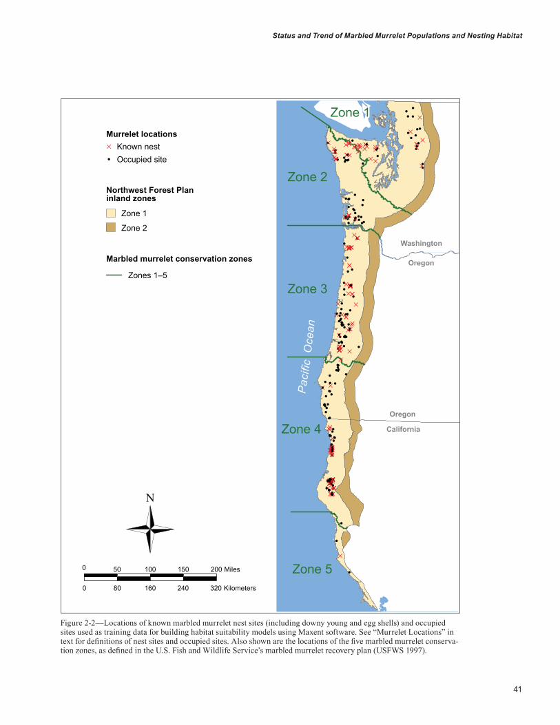
41
Status and Trend of Marbled Murrelet Populations and Nesting Habitat
!
D
!D!DD!
!!!DD DD! DD!!!
!!DDDDDD!!D!!!!!!D!!!DDD!DDD!!!DDDDD!DDD!
!!!DDD!!DDDDDDDDDD!!!!!DD!!
!D!!
!!
!D!DD
D
DDDDDDDDDD
D!
!
!
!
!
!
!
!
!
!
!!
!!
!!
!
!!!!!
!!!!
D! D!!!
! !
!!!!!!
D
DDDDDDD!D !DDDD!!!!
!!!! !D!D!DD!!
!! D! !D!!!!! DD!D D!!!
!!
D!
!! DDD!DDDDDDDDDD!DD!
!
!
DD
!
DDDDDDDDDDDDDDDDDD!
!DDDD
D
D
!
!
!! !! !! !D! !!D !D!! !DDD!!!
!!
!!!!
!
!D!!
! D!!!!DDDDDDDD D!D !DDD!! DDDD! D!D DD !! DDD DDD DD !DDD DD! DDDDDDD !!D D ! D
!!
!D!!
D!!
!!Zone 1
Zone 2
Zone 5
Zone 4
Zone 3
California
Oregon
Washington
Oregon
Pac
ific
Oce
an
0 50 100 150 200 Miles
0 80 160 240 320 Kilometers
D
!
Zones 1–5
Murrelet locationsKnown nestOccupied site
Northwest Forest Planinland zones
Marbled murrelet conservation zones
Zone 1
Zone 2
Figure 2-2—Locations of known marbled murrelet nest sites (including downy young and egg shells) and occupied sites used as training data for building habitat suitability models using Maxent software. See “Murrelet Locations” in text for definitions of nest sites and occupied sites. Also shown are the locations of the five marbled murrelet conserva-tion zones, as defined in the U.S. Fish and Wildlife Service’s marbled murrelet recovery plan (USFWS 1997).

42
GENERAL TECHNICAL REPORT PNW-GTR-933
Updates to the original 1994 LUA geographic informa-tion system (GIS) map were produced in 2002, 2009, and 2013 for the 10-year, 15-year, and 20-year monitoring reports, respectively. Each successive update improved the accuracy of some of the mapped allocation boundaries based on subse-quent work by individual federal entities, as well as corrected some mapping anomalies and inconsistencies (i.e., “gaps” and “slivers”) that had been inadvertently introduced during earlier mapping efforts. More importantly, these updates incorporated major allocation changes that had occurred since the previous mapping effort. Examples of these types of changes include the designation of new wilderness areas and land swaps between federal and nonfederal entities.
Each update represents a significant amount of time and effort on the part of monitoring team personnel, who made every effort to procure and incorporate the best available data at that time. The current (2013) version of the LUA map (fig. 2-1) represents the cumulative result of these three updates. Even so, some issues and limitations remain. These include the inability to map NWFP riparian reserves (which can cover significant amounts of land where stream densities are high) and inconsistencies in how administratively withdrawn areas (e.g., withdrawn from the acres available for timber harvest at the discretion of individual national forests) were mapped (Davis and Lint 2005, Huff et al. 2006a). The lack of mapped NWFP riparian area is because, as Moeur et al. (2005) noted, “…at the Plan scale, they cannot be reliably distinguished from [the adjacent nonreserved or matrix [lands] because of a lack of consistency in defining intermittent stream corridors and varying definitions for riparian buffers.” As those authors observed, this affects only NWFP riparian reserves that are not within another NWFP reserve type (such as late-succes-sional reserve) This limitation has no effect on the Maxent model, or on the suitability class assigned to any area, but would affect whether habitat in a riparian area on federal lands is classified as “reserved” or “nonreserved.” This would result in our estimates for reserved federal lands being biased low and estimates for federal nonreserved lands being biased higher by the same amount, than if riparian reserves were mapped. The NWFP initially estimated the amount of riparian reserve within nonreserved LUAs to represent about 32 percent of the nonreserved LUA area of federal lands
(USDA and USDI 1994a). Our analyses (below) assigned about 9 percent of the higher suitability murrelet nesting habitat on NWFP federal lands to “nonreserved” LUAs, for the baseline year. Applying the 32 percent estimate to the 9 percent of habitat on nonreserved federal lands suggests that about 3 percent of higher suitability habitat in federal riparian reserves would be incorrectly classified as nonreserved; this provides a rough estimate of the potential error resulting from the lack of mapped riparian reserves. Another minor issue involves a small amount of federally owned lands that are awaiting official land use allocation designation. These areas, which represent about 0.1 percent of the total area modeled, are identified as “not designated” in the 2013 map and are reported in the nonreserved category in this report.
Land use allocations within the NWFP area will con-tinue to change. We plan to update the LUA map with the intent of improving it for each successive monitoring effort. Previous versions of the LUA map have been archived, and for monitoring purposes, we always report vegetation and habitat changes within the reference frame of the most up-to-date version.
Data Sources for CovariatesGNN covariates—Many of the covariates used in our habitat-suitability models were based on GNN maps of forest composition and structure (Ohmann and Gregory 2002). The GNN maps were developed specifically for landscape- and regional-scale analysis and monitoring in forest ecosystems (Moeur et al. 2005, 2011; Ohmann and Gregory 2002; Spies et al. 2007). As part of the NWFP Effectiveness Monitoring program, scientists mapped detailed attributes of forest composition and structure for all forested land in the NWFP area using GNN imputation; the GNN method integrates vegetation measurements from regional grids of field plots, mapped environmental data, and Landsat imagery to ascribe detailed ground attributes of vegeta-tion to each pixel in a digital landscape map (Ohmann and Gregory 2002; Ohmann et al. 2010, 2014). The GNN method also provides a suite of diagnostics detailing model reliability and map accuracy (see app. 5 in Davis et al. 2015 for a summary). The GNN analyses created attribute maps
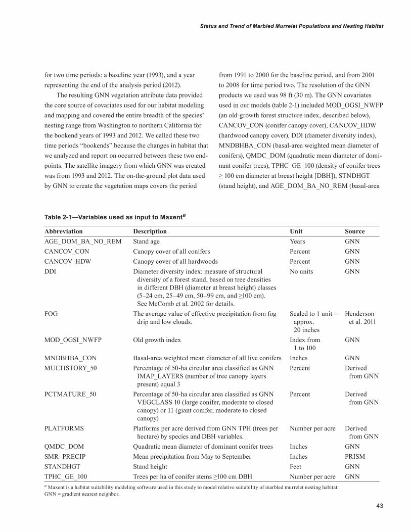
43
Status and Trend of Marbled Murrelet Populations and Nesting Habitat
for two time periods: a baseline year (1993), and a year representing the end of the analysis period (2012).
The resulting GNN vegetation attribute data provided the core source of covariates used for our habitat modeling and mapping and covered the entire breadth of the species’ nesting range from Washington to northern California for the bookend years of 1993 and 2012. We called these two time periods “bookends” because the changes in habitat that we analyzed and report on occurred between these two end-points. The satellite imagery from which GNN was created was from 1993 and 2012. The on-the-ground plot data used by GNN to create the vegetation maps covers the period
from 1991 to 2000 for the baseline period, and from 2001 to 2008 for time period two. The resolution of the GNN products we used was 98 ft (30 m). The GNN covariates used in our models (table 2-1) included MOD_OGSI_NWFP (an old-growth forest structure index, described below), CANCOV_CON (conifer canopy cover), CANCOV_HDW (hardwood canopy cover), DDI (diameter diversity index), MNDBHBA_CON (basal-area weighted mean diameter of conifers), QMDC_DOM (quadratic mean diameter of domi-nant conifer trees), TPHC_GE_100 (density of conifer trees ≥ 100 cm diameter at breast height [DBH]), STNDHGT (stand height), and AGE_DOM_BA_NO_REM (basal-area
Table 2-1—Variables used as input to Maxenta
Abbreviation Description Unit SourceAGE_DOM_BA_NO_REM Stand age Years GNNCANCOV_CON Canopy cover of all conifers Percent GNNCANCOV_HDW Canopy cover of all hardwoods Percent GNNDDI Diameter diversity index: measure of structural
diversity of a forest stand, based on tree densities in different DBH (diameter at breast height) classes (5–24 cm, 25–49 cm, 50–99 cm, and ≥100 cm). See McComb et al. 2002 for details.
No units GNN
FOG The average value of effective precipitation from fog drip and low clouds.
Scaled to 1 unit = approx. 20 inches
Henderson et al. 2011
MOD_OGSI_NWFP Old growth index Index from 1 to 100
GNN
MNDBHBA_CON Basal-area weighted mean diameter of all live conifers Inches GNNMULTISTORY_50 Percentage of 50-ha circular area classified as GNN
IMAP_LAYERS (number of tree canopy layers present) equal 3
Percent Derived from GNN
PCTMATURE_50 Percentage of 50-ha circular area classified as GNN VEGCLASS 10 (large conifer, moderate to closed canopy) or 11 (giant conifer, moderate to closed canopy)
Percent Derived from GNN
PLATFORMS Platforms per acre derived from GNN TPH (trees per hectare) by species and DBH variables.
Number per acre Derived from GNN
QMDC_DOM Quadratic mean diameter of dominant conifer trees Inches GNNSMR_PRECIP Mean precipitation from May to September Inches PRISMSTANDHGT Stand height Feet GNNTPHC_GE_100 Trees per ha of conifer stems ≥100 cm DBH Number per acre GNNa Maxent is a habitat suitability modeling software used in this study to model relative suitability of marbled murrelet nesting habitat.GNN = gradient nearest neighbor.
44
GENERAL TECHNICAL REPORT PNW-GTR-933
weighted stand age based on dominant and codominant trees, and excluding remnant trees). The GNN attributes also contributed to other covariates, as described below.
For both the 15- and 20-year reports, the GNN covariate maps were developed using Landsat time-series data that were temporally normalized using the LandTrendr algorithm as described below. The GNN covariate data used for the 20-year report included several incremental improvements over the 15-year data and methods as summarized below, some of which were also documented in Ohmann et al. (2014):• Newfieldplotsadded: The 15-year maps were
based on plots measured through 2007. The 20-year GNN products included four more years of field plot data, measured through 2011.
• Screeningforfieldplotoutliers: This process benefited immensely from having yearly time-series mosaics from 1984 to 2012, as well as LandTrendr disturbance maps, to aid in determination of timing of disturbances relative to plot measurement. In screen-ing, potential outlier plots were flagged using various algorithms that compared observed plot attributes to the predicted map attributes to identify mismatches. These plots were viewed in the LandTrendr imagery and digital aerial photography to identify and exclude plots that straddled contrasting forest conditions (e.g., older forest and clearcut), or that had been disturbed between plot measurement and imagery dates.
• New spatial predictor: Spatial predictor variables normally used in the GNN process include maps of abiotic variables such as climate, topography, lati-tude, and longitude, as well as Landsat imagery of tasseled cap brightness, greenness, and wetness. For the 20-year report, analysts added the normalized burn ratio (NBR), which is a vegetation index used as a form of change detection. By comparing the NBR before and after a fire or other disturbance event, one can identify the change brought about by that event.
• Matching of plots to imagery: For the 15-year report, we had only two LandTrendr imagery dates to work with, and plots were matched either to imagery time 1 or time 2. This resulted in as much as a 6-year differ-ence between plot measurement date and imagery date.
Many plots were excluded from modeling because of disturbance between plot and imagery dates. For this 20-year report, the GNN analysis implemented yearly matching of field plots to LandTrendr data, with plots matched to the same imagery year as plot measurement. This was made possible by having yearly LandTrendr mosaics available from 1984 to 2012. This resulted in many fewer plots excluded because of disturbance, and effectively eliminated differences between plot and imagery dates associated with growth.
Although GNN was designed for regional-scale analyses, the maps portrayed forest structure and compo-sition at finer spatial scales. In a recent assessment of the MOD_OGSI_NWFP covariate, GNN performed well at the scale of a 30-km hexagon (distance from the center of one hexagon to the next), which covered slightly over 190,000 ac (Ohmann et al. 2014). More information on the GNN mapping for the NWFP, and map products, are available at http://lemma.forestry.oregonstate.edu/projects/nwfp.
Platform covariate—Marbled murrelets in the NWFP area most often nest on larger limbs of coniferous trees. This type of nest location is termed a “platform,” and the presence and abundance of platforms are very often good predictors of suitable mur-relet nesting habitat (Burger 2002, Burger et al. 2010, Nel-son 1997). The PLATFORM covariate was computed from the GNN data using data from previous studies (Raphael, n.d.) in which numbers of platforms were counted on a very large sample of trees from plots scattered throughout the murrelet range, and then summarized by tree species and diameter class (Raphael et al. 2011). We computed mean numbers of platforms by tree species and DBH class, and then applied these means to tree counts from the GNN data. The mean number of platforms for each species and DBH group (table 2-1 in Raphael et al. 2011) was multiplied by the associated GNN attribute data on conifer trees per hectare (e.g., TPH_PSME_50_75 for density of Douglas-fir trees in the 50- to 75-cm DBH class) to estimate total number of platforms per acre. This latter number was used as the covariate value. Although the abundance of plat-forms is likely important for nest habitat quality and nest
45
Status and Trend of Marbled Murrelet Populations and Nesting Habitat
site selection, other ecological and environmental factors such as vegetative cover, stand characteristics, and local climate may also be important in nest site selection (Nelson 1997). For this reason, we included covariates that repre-sented other factors that could also be important to habitat suitability and nest site selection by murrelets.
Old-growth structure index covariate (MOD_OGSI_NWFP)—The “old-growth structure index” (OGSI) was conceptu-ally developed by Spies and Franklin (1988) and further refined by Franklin and Spies (1991). Specifically, it was designed to reflect the continuous nature of ecological succession as opposed to identifying one point along a continuum to separate old growth from younger forests (Franklin and Spies 1991). The OGSI consists of measur-able forest structure elements, in our case: (1) density of large live trees, (2) diversity of live tree size classes, (3) density of large snags, and (4) percentage cover of down woody material. These are elements commonly considered as key ecological and structural attributes of old-growth forests within the NWFP area. Low index values repre-sented younger or less structurally complex forests and high index values represented older or more structurally complex forests. The OGSI covariate we used was based on attribute data provided by GNN, and calculated separately for different forest vegetation types or zones, to account for structural differences among forest types, such as what diameter constitutes a “large” tree. Davis et al. (2015) developed the OGSI covariate we used, and their publication provides additional details. Whereas Davis et al. (2015) conducted further analyses using the OGSI variable to identify older, late-successional forests at different stages of stand development, we used the variable more simply as continuous input covariate in our habitat models.
Landscape covariates—Previous studies (Meyer and Miller 2002; Raphael et al. 1995, 2011) found that murrelets select larger patches of contiguous forest for nesting. To address patch charac-teristics, we created two covariates, MULTISTORY_50 and PCTMATURE_50. These covariates were derived
from GNN IMAP_LAYERS and VEGCLASS covariates, respectively. For each pixel, we evaluated forest condition on a 50-ha (124-ac) circular neighborhood centered on the pixel, assigning the percentage of the circle in mature-forest condition to the pixel (see table 2-1).
Fog covariate—We included FOG as a covariate because cool summer fog can greatly moderate summer temperatures and humidity near the coast, especially in northern California, where fog plays an important ecological role in the distribution of coast redwood (Sequoia sempervirens (lamb ex D. Don) Endl.) forest (Sawyer et al. 2000) with which murrelets are closely associated (Meyer et al. 2002). Fog may also create suitable conditions for the development of epiphytes on branches, contributing to potential murrelet nesting plat-forms. The fog spatial layer was developed by Henderson et al. (2011) and represents the average value of effective precipitation added by fog drip and low clouds. One unit of “fog effect” equals 508 mm (20 in) of effective precip-itation. We included FOG in the Oregon and Washington model regions, in part, to maintain consistency in covari-ate sets across the NWFP area.
Climate covariates—We obtained monthly 30-year normal (1981–2010) raster climate data (800-m resolution) from PRISM models (PRISM Climate Group 2012), including July maximum temperature (JULY_MAXT) and mean precipitation for the months from May through September. We averaged these five monthly mean precipitation models to produce a mean summer precipitation model (SMR_PRECIP).
Other Data SourcesWe used 2009 versions of the physiographic province layer (which also defines the NWFP area) (FEMAT 1993) and the marbled murrelet range layer to define the extent of our analysis, and report outcomes based on these areas. Revi-sions to the original FEMAT (1993) physiographic province layer involved correction of state boundaries using 1:24,000-scale digital topographic maps and inclusion of a more detailed, higher resolution coastline, which included several islands that were previously omitted. Revisions to the 2004
46
GENERAL TECHNICAL REPORT PNW-GTR-933
version of the murrelet range layer were confined to inclu-sion of the higher resolution coastline. The murrelet’s range south of Canada was divided into the six marbled murrelet “conservation zones” identified in the species’ recovery plan (USFWS 1997), and the conservation zones were further broken into strata for purposes of population monitoring (Miller et al. 2006, Raphael et al. 2007). Five of these conservation zones (1 through 5) overlap the NWFP area. We extended inland the breaks between conservation zones and strata, primarily by following watershed lines, so that we could summarize nesting habitat data and examine rela-tionships between inland nesting habitat and at-sea murrelet populations at the scale of conservation zones (fig. 2-2).
As described elsewhere in this report, our habitat modeling excluded NWFP Inland Zone 2 in Oregon and California because of the scarcity or lack of known murrelet nest and occupied sites from those areas. Additionally, other data indicate that murrelets rarely nest in NWFP Inland Zone 2 in Oregon and California (Alegria et al. 2002, Hunter et al. 1998).
Covariate Selection and Screening From the literature (including Raphael et al. 2011) and our experience, we selected a candidate set of environmental covariates. In contrast to the 15-year analysis, we did not eliminate correlated variables because our intent was to use the available data to produce the strongest predictive accuracy of habitat suitability, and we were less interested in describing the environmental drivers of murrelet distribution and habitat (Baldwin 2015, Merow et al. 2013). For this same reason, we used the same full set of covariates in each model-ing region. Our final covariate list is summarized in table 2-1.
Accuracy AssessmentWhen screening potential GNN covariates, we considered accuracy assessment data provided by the GNN/IMAP project. The assessments used a form of ground-truthing, by comparing observed values for a grid of field inventory plots with the GNN-predicted (modeled) values for those same plots. This provided accuracy data for nine GNN attributes used directly in our models, as well as for OGSI_NWFP, upon which the MOD_OGSI_NWFP covariate is based
(table 2-2). Accuracy assessments were not available for non-GNN covariates or for derived GNN covariates, but were available for some GNN attributes which contributed to the PCTMATURE_50 covariate. GNN accuracy assess-ments are available at http://lemma.forestry.oregonstate.edu/data/structure-maps.
Table 2-2 summarizes, by GNN modeling region, the accuracy assessment results for GNN attributes that contributed directly or indirectly to model input covariates. Accuracy, as measured by correlation “r” values, ranged from 0.37 to 0.81 among modeling regions for the eight attributes used directly as covariates, plus the three that were the basis for the PCTMATURE_50. When averaged across the four modeling regions, covariate accuracy ranged from r values of 0.56 to 0.75 for covariates, and averaged lowest in the California Coast region, where the sample size of field inventory plots was smaller.
The PLATFORM covariate was based in part on GNN attribute data on tree density by species and DBH class. Creating these required the tree density data to be subdi-vided into 30 categories for each modeling region (five DBH classes for each of six species groups). Accuracy assess-ments were not available for these categories; however, trees ≥100 cm DBH contribute the most to platform numbers, and when all conifers of this size class were pooled (TPHC_GE_100), accuracy data are available, with correlations ranging from 0.48 to 0.67 (table 2-2). Thus, accuracy was moderately high for the pooled set of large conifer trees that provide the greatest number of platforms.
Data PreparationAll covariates were processed as ArcGIS (ESRI 1999-2013) rasters at 30-m resolution, the native resolution of the GNN data. A smoothing function (focal mean) was applied to all covariate rasters, except MULTISTORY_50 and PCTMATURE_50, to assign the mean value of the 3 × 3-pixel neighborhood to the cell. We used this smoothing function to reflect the spatial uncertainty in our murrelet location data, but still maintained a spatial resolution <1 ha. All covariate rasters were converted to ASCII files for input into Maxent and Maxent ASCII output back to rasters using ArcGIS.

47
Status and Trend of Marbled Murrelet Populations and Nesting Habitat
Tabl
e 2-
2—A
ccur
acy
asse
ssm
ent d
ata
for g
radi
ent n
eare
st n
eigh
bor (
GN
N) a
ttri
bute
s us
ed a
s co
vari
ates
in m
urre
let n
est h
abita
t m
odel
ing
Correlationcoefficientsb
yGNNmodelingregion
Was
hing
ton
Coa
st
Ran
ge a
nd C
asca
des
Ore
gon
Coa
st
Ran
geO
rego
n an
d C
alifo
rnia
—K
lam
ath
Cal
iforn
ia
Coa
st R
ange
Cov
aria
teG
NN
att
ribu
teR
MSE
Cor
rela
tion
coefficient
RM
SEC
orre
latio
n coefficient
RM
SEC
orre
latio
n coefficient
RM
SEC
orre
latio
n coefficient
Con
ifer c
anop
y co
ver
CAN
CO
V_C
ON
0.21
0.78
0.28
0.78
0.39
0.73
0.46
0.69
Har
dwoo
d ca
nopy
cov
erCA
NC
OV_
HD
W1.
430.
700.
800.
650.
720.
700.
480.
61Tr
ee d
iam
eter
div
ersit
y in
dex
DD
I0.
330.
780.
340.
770.
370.
690.
350.
61B
asal
-are
a w
eigh
ted
mea
n di
amet
er a
t bre
ast h
eigh
t (D
BH),
all c
onife
rs
MN
DBH
BA_C
ON
0.43
0.72
0.47
0.73
0.52
0.52
0.66
0.39
Qua
drat
ic m
ean
DBH
, do
min
ant a
nd c
odom
inan
t co
nife
rs
QM
DC
_DO
M0.
440.
710.
470.
740.
560.
510.
700.
37
Con
trib
utor
s:PC
TMA
TUR
E_50
QM
DA
_DO
M0.
400.
750.
400.
790.
510.
550.
540.
51CA
NC
OV
0.19
0.75
0.19
0.80
0.26
0.75
0.19
0.78
Old
-gro
wth
stru
ctur
e in
dex
MO
D_O
GSI
_NW
FP0.
510.
680.
500.
700.
570.
510.
590.
42St
and
heig
ht, d
omin
ant a
nd
codo
min
ant t
rees
STN
DH
GT
0.38
0.71
0.33
0.81
0.47
0.58
0.45
0.55
Bas
al-a
rea
wei
ghte
d st
and
age,
exc
ludi
ng re
mna
nt tr
ees
AG
E_D
OM
_BA
_NO
_REM
0.55
0.77
0.55
0.76
0.51
0.59
0.64
0.46
Con
ifer t
rees
per
hec
tare
≥1
00 c
m D
BHTP
HC
_GE_
100
1.91
0.58
1.66
0.67
1.70
0.52
2.28
0.48
Tota
l inv
ento
ry p
lots
use
d in
G
NN
mod
el d
evel
opm
ent
2,93
72,
024
3,70
397
5
Val
ues p
rese
nted
are
nor
mal
ized
root
mea
ns sq
uare
err
or (R
MSE
) and
cor
rela
tion
coef
ficie
nts (
‘r’) f
or in
divi
dual
GN
N m
odel
ing
regi
ons.
Thes
e in
clud
e ni
ne a
ttrib
utes
use
d di
rect
ly a
s co
varia
tes,
and
two
GN
N a
ttrib
utes
that
con
trib
uted
tow
ard
the
PCTM
ATU
RE_
50 c
ovar
iate
s.
48
GENERAL TECHNICAL REPORT PNW-GTR-933
Murrelet LocationsWe used agency records to identify two types of murrelet nest locations to serve as species presence sites for training the Maxent models: known nest locations, and stand loca-tions where murrelet occupancy behavior was observed dur-ing audiovisual surveys of potential habitat (Evans Mack et al. 2003), using all available records through 2013. In both cases, we used only records in which inspection of digital aerial photographs confirmed that undisturbed forest was present at the location in 1993, our baseline modeling year. As described in a previous report (Raphael et al. 2011), we initially focused on known nest locations, but this yielded relatively small sample sizes and did not always provide representative spatial distribution across potential murrelet habitat. Therefore, we added a random sample of “occupied” sites equal in number to the sample of nest sites for each state. We used an equal number of occupied and nest sites to minimize any potential bias in one dataset or the other, as neither dataset was collected via random sampling and may have biases. For example, many of the occupied sites were surveyed prior to timber harvest, so site selection for these surveys was guided by timber considerations. We assumed that, when pooled, the nest and occupied location data used in our habitat modeling represented the breadth of possible murrelet habitat types (McShane et al. 2004, Nelson et al. 2006, Raphael et al. 2006). These known nest and occupied location data (fig. 2-2) were used to train the Maxent habitat suitability model.
Location data for known nest and occupied sites were collected from a variety of sources. In Washington, the source was a database maintained by the Washington Department of Fish and Wildlife. California sources included a database maintained by the California Depart-ment of Fish and Wildlife, supplemented by records assem-bled by the U.S. Fish and Wildlife Service, and also included a number of nests located by a radiotelemetry study (Hebert and Golightly 2008). For Oregon, data sources were from a database currently maintained by Oregon State University and populated with records from the U.S. Forest Service, the BLM, the Oregon Department of Forestry, Oregon Parks and Recreation Department, and Oregon State University (Nelson 2015).
For known nest locations, we included (1) known nest trees located by visual observations and by radiotelemetry of nesting murrelets (n = 134); (2) sites where downy, flightless murrelets had been found on the ground (n = 7): and (3) sites where murrelet eggshells had been found on the ground, typically at the base of a suitable nest tree (n = 43). Numbers of locations of downy young plus eggshells were 9, 4, and 33 in Washington, Oregon, and California, respectively. For the occupied sites, behaviors are con-sidered evidence of nesting at or near the location of the behavior (Evans Mack et al. 2003). For our analyses, these behaviors included one or more of the following: murrelets circling at or below the forest canopy; circling above the canopy by no more than 1.0 canopy height; flying through in a straight flight path below the canopy; landing in, perching, or departing from a tree; or birds emitting ≥3 calls from a fixed point in a tree within 100 m (328 ft) of an observer (Evans Mack et al. 2003).
We manually screened the data on known nest site locations with the aid of aerial photography, base GNN vegetation mapping data, and communications with original data sources to confirm and correct locations and remove duplicate records. We further screened the data so that all presence locations included in the final dataset were greater than 30 m apart (the resolution of our modeling).
The selection of occupied sites used to train the Maxent model involved a series of filters and screenings. Filters were used to eliminate duplicate sites and those that fell within 164 ft (50 m) of a known nest site. Additionally, the Washington and Oregon databases were so robust (4,900+ and 4,300+ records, respectively) that a filter was applied to randomly eliminate sites within 5,774 ft (1760 m) of each other. This was done to maximize the distribution of the points among different habitat stands, as well as to reduce the number of records in the databases to a more manage-able size for the manual screening process. The subset of occupied sites produced by the filtering process was then screened by manual inspection of each site location using digital aerial photography. Sites were eliminated if forest conditions at the site were clearly nonhabitat (e.g., clearcut, young forest, roadway, open water) in the baseline year. In total, about 20 percent of potential occupied sites were

49
Status and Trend of Marbled Murrelet Populations and Nesting Habitat
eliminated in this last process. Finally, a stratified random selection was made from the remaining sites equal to the number of known nest sites within a state, and stratified by physiographic provinces within states proportional to the amount of habitat-capable lands in each province. In Oregon and California, we limited our habitat analysis to the NWFP Inland Zone 1 (fig. 2-2) because of the scant evidence for murrelet use of inland areas (Alegria et al. 2002, Hunter et al. 1998). In California, we found no records of murrelet use of NWFP Inland Zone 2. In Oregon, there are nine known occupied sites in NWFP Inland Zone 2 that are all clustered near the boundary with NWFP Inland Zone 1 in a small area near Roseburg. Elsewhere in Oregon, data are lacking (no surveys conducted or data not available in database); an exception is the Siskiyou Mountains in the southern end of the state, where surveys found negligible use in NWFP Inland Zone 2 (no detections in 3,300 survey visits, Alegria et al. 2002). In Washington, the occupied sites from NWFP Inland Zone 2 were much more evenly distributed spatially and with respect to distance from the coast, and we decided to include NWFP Inland Zone 2 in our analysis area.
Habitat ChangeWe used two methods to assess change in the amount and distribution of habitat from the 1993 baseline to current conditions (2012). For the first method (the “bookend approach”), we compared amounts of habitat estimated by the Maxent models for two time periods: (1) the baseline year, and (2) 2012, which we obtained by projecting the Maxent model from the baseline period onto a map of the covariate values for 2012. Projecting the model in this manner could result in a projected model with validity issues if covariate values in the 2012 data were outside the range of covariate values in the baseline study area used to build the Maxent model (Phillips et al. 2006). However, all covariate values were within the range of baseline values. Using this approach, we estimated net change during the period, which represented the difference between area of nesting habitat gains (change in Maxent score from below to above our threshold) and losses (change in Maxent score from above the threshold to below that threshold). Our second approach, “LandTrendr-verified,” used both the bookend model loss
results and LandTrendr data to estimate habitat loss from the baseline condition, and to identify causes of observed losses.
For the second approach, we calculated losses as follows: first, we used the Maxent bookend model results from each state to identify areas that had changed from “suitable” to “unsuitable” habitat during the analysis period. We then examined these bookend losses spatially by using a reclassification of the LandTrendr change maps (see below) from the same time period, which identified four distur-bance types: wildfire, timber harvest (primarily harvest, but can include short-term disturbances other than fire and harvest), insects and disease (and other long-term distur-bance agents), and other natural disturbance. Lands within our study area that were not classified by LandTrendr were assumed to have ‘no disturbance.’ As described below, the “other natural disturbance” class was used only in Congres-sionally Reserved or Administratively Withdrawn (CRAW) lands, which primarily comprise national parks, wilderness areas, and national wildlife refuges, plus other federal lands identified for uses which do not include timber harvest. We considered bookend losses that overlapped one of the four disturbance classes as “verified” by LandTrendr. If both the bookend analyses indicated a loss of suitable habitat for that pixel and the LandTrendr data also indicated a disturbance, it was assigned a particular disturbance type.
Differences between these two methods of estimat-ing habitat change are as follows: (1) for the “bookend approach,” we used the net change in habitat as a result of gains and losses, while the “LandTrendr-verified approach” estimated only losses, and (2) the latter method used information from two sources (the Maxent models and LandTrendr) to estimate losses, and provided data on cause of habitat loss. The strengths and weaknesses of the two approaches are addressed in the “Discussion” section of this chapter.
LandTrendr Change DetectionDavis et al. (2015) provide a detailed description of this topic, which is summarized here. The annual time-series of LandTrendr-generated maps identified where, when, how much, and how long disturbances had occurred between 1993 and 2012. They also showed areas where
50
GENERAL TECHNICAL REPORT PNW-GTR-933
the forest vegetation had been stable or was recovering. These time-series maps of forest vegetation disturbance and recovery were similar to what was used in the 15-year monitoring reports. They were developed following meth-ods in Kennedy et al. (2010, 2012) and verified for accuracy using the TimeSync method (Cohen et al. 2010). The LandTrendr maps represented three aspects of vegetation change: (1) year of disturbance, (2) magnitude of distur-bance, and (3) duration of disturbance. Davis et al. (2015) further classified disturbances identified by these maps to produce a map of where timber harvesting, wildfire, insect and disease, and other natural disturbances (e.g., blow-down, floods, landslides, etc.) occurred between 1993 and 2012 (see app. 4 in Davis et al. 2015 for details). Where this map overlapped losses of suitable murrelet nesting habitat, it helped to explain the causes for habitat loss since the NWFP’s implementation.
Landsat imagery for the NWFP area was acquired from the USGS Glovis website for the summer period (usually July and August) from 1984 to 2012. Images were atmospherically corrected (Masek et al. 2008) and, to minimize cloud coverage, multiple image dates within a given season were used to produce a clear-pixel composite image for that year.
The composite imagery was then processed using the LandTrendr segmentation algorithm (Kennedy et al. 2010), which computes the NBR spectral index for each pixel in the time-series. The NBR (Key and Benson 2006; van Wagtendonk et al. 2004) is a vegetation index for which change in NBR can be used to detect vegetation change. By comparing the NBR before and after a fire or other dis-turbance event, one can identify the magnitude of change brought about by that event. The algorithm identified year-dates (vertices) where changes in NBR had occurred (normally associated with changes in vegetation). Between vertices, temporal segments were established and each segment was labeled as disturbance, recovery, or stable based on spectral direction. These data were used by Davis et al. (2015) to identify the year and duration of dis-turbance. For each segment, Davis et al. (2015) estimated the percentage of vegetation cover for the beginning and ending vertices using a statistical model that relates NBR
to vegetation cover (Cohen et al. 2010). The difference between vertex predictions represented the magnitude of the disturbance or recovery for that segment in terms of percentage of vegetation cover. Finally, the absolute mag-nitude was scaled to the starting value to compensate for varying predisturbance forest cover values, such that all magnitudes were expressed as a proportion of the starting condition. The final step was to spatially filter the pixels to a minimum mapping unit of 11 pixels, or about 1 ha. For a given area, the change detection analysis used the highest magnitude disturbance that occurred throughout the time series. Kennedy et al. (2012) found overlapping distur-bances to be rare in the NWFP area, covering less than 5 percent of the area of primary disturbances.
The next step in identifying causes of disturbance was to separate short-duration events, such as timber harvest, from slower, longer duration causes such as insect damage. An analysis of wildfire and timber harvest unit polygons showed an average disturbance duration signal of about 1.5 ± 1.0 years (mean ± 1SD) for regeneration (e.g., clear-cut) harvests, 1.7 ± 1.7 years for wildfires, and 2.2 ±2.2 years for thinning harvests (Davis et al. 2015). Based on this information, the duration map was classified into a binary map of fast (1-to 4-years duration) and slow (>4 years) disturbance. Fast disturbance represented abrupt events such as a wildfire, timber harvest, wind blowdown, or debris flow. Slow disturbances represented insects or disease, or postfire mortality. To help identify wildfire disturbances, Davis et al. (2011; 2015) used maps of the perimeters of wildfires that occurred between 1993 and 2012. The maps of wildfire disturbance are fairly inclusive of all major wildfires exceeding a few acres, but the many wildfires smaller than this were not mapped. Insect damage detection data (USDA FS 2008) helped classify insect-caused disturbance. Finally, LUAs helped identify areas (CRAW lands) of fast disturbance where timber harvest was unlikely. Agency “forest activity” GIS layers were used where available to identify harvest areas, but similar GIS layers were not available for timber harvest on non-federal lands. Davis et al. (2015; app. 4) provide a complete classification rule set used to produce the map of cause of disturbance and classification accuracy assessment.
51
Status and Trend of Marbled Murrelet Populations and Nesting Habitat
The disturbance maps did not capture all disturbances that occurred during the final year of our analysis (2012), particularly for those disturbances that occurred in 2012 after the satellite image acquisition date, or that were obscured by smoke from wildfires. Those changes will be captured in subsequent monitoring efforts. Our disturbance classification map provides a general sense of the amount and change agents behind losses of suitable murrelet nesting habitat between 1993 and 2012.
Specific criteria used to identify causes of change were:
Timber harvest. Represents timber harvesting; including thinning and regeneration harvests. Classified as fast (dura-tion ≤4 years) disturbances outside of CRAW lands and also outside of wildfire perimeters; or if within a wildfire perime-ter, then predating the fire year by more than two years. Some fast disturbances meeting these criteria occurred within areas identified as having insect damage. Visual inspection with high resolution aerial imagery indicated that most of these disturbances were from timber harvesting, some likely related to insect damage salvage (Davis et al. 2015). Due to a lack of spatial data on landslides, floods and blowdown, the ‘timber harvest’ category includes some fast disturbances owing to those other causes, when located outside of CRAW lands.
Wildfire. Fast or slow (duration >4 years) disturbances within a mapped wildfire perimeter, but only when no other disturbance preceded the fire year. Slow disturbance within wildfire perimeters likely represent post-fire mortality.
Insect and disease. Slow-duration disturbances that oc-curred outside of wildfire perimeters, or if within a wildfire perimeter, preceded the fire year. Also includes fast distur-bances that occurred within areas identified as having insect damage, where mapped for two or more consecutive years.
Other natural disturbance. Fast disturbances that oc-curred within CRAW lands and outside of wildfire perim-eters, or if within fire, then preceded fire year. Includes blowdown, floods, and landslides. Due to the lack of data that would allow us to distinguish timber harvest from other fast natural disturbances (other than fire), this cause was only used within CRAW lands, where timber harvest was very unlikely.
Model RefinementsOnce we selected our final set of covariates, we conducted a series of Maxent model runs to evaluate model performance. To evaluate model performance, we used training and test model gain, and area under the curve statistics (AUC; Field-ing and Bell 1997, Boyce et al. 2002). Gain is closely related to deviance, a measure of goodness of fit used in generalized additive and generalized linear models and is available as part of the model output in Maxent (Phillips et al. 2006). The lowest value of gain is 0 and gain usually increases toward an asymptote as the fit between the model and the training data improves. During a run, Maxent is generating a probability distribution over pixels in the grid, starting from a uniform distribution and repeatedly improving the fit to the data. The gain is defined as the average log probability of the presence samples, minus a constant that makes the uniform distribu-tion have zero gain. At the end of a run, the gain indicates how closely the model is concentrated around the presence samples; for example, if the gain is 2, it means that the aver-age likelihood of the presence samples is exp(2) ≈ 7.4 times higher than that of a random background pixel (Phillips, unpublished tutorial, available at http://www.cs.princeton.edu/~schapire/maxent/). For a given model run, separate gain statistics were generated for the training (75 percent) and test (25 percent) portions of the available presence sites.
The other measure of model performance, AUC, is the area under a ROC (receiver operator characteristic) curve (Boyce et al. 2002, Hirzel et al. 2006). AUC is a measure of model performance that illustrates how well one can dis-tinguish presence sites from the available background sites (some of which are likely to be occupied by and/or suitable for murrelets). Values range from 0 to 1.0 and location data that cannot be distinguished from the background with any greater probability than a random coin toss would yield an AUC score of 0.5. We present AUC values generated using test data, which is data held back during model development and then used to test model fit and accuracy. Test AUC provides a measure of model performance in classifying an independent set of presence points.
Maxent also provides a choice of covariate relation-ships to include in a model, called “features.” Feature types include Linear, Quadratic, Threshold, Hinge, and Product.
52
GENERAL TECHNICAL REPORT PNW-GTR-933
These features set the possible shapes of the relationship between a covariate and the response (i.e., the Maxent probability distribution) or allow for covariate interactions (product features). A user can select any combination of these feature types. A model with linear features requires the fewest parameters, as only two parameters (slope and intercept) are estimated for each covariate. Quadratic relationships require both slope and intercept as well as exponent parameters for each covariate. Hinge features create a piece-wise approximation to any distribution. The number of parameters for any one covariate increases for each “hinge” in the modeled distribution, which can result in a complex distribution and many parameters. The Product feature allows for interactions among all pairs of covariates. The total number of parameters for any model depends, therefore, on the types of features selected and the complexity of the response curves between the covar-iates and the probability scores. In addition, Maxent has a “regularization” constant that can be specified. Increasing the regularization value above the default has the effect of smoothing the response curve, thereby reducing the number of parameters in the model. Regularization is a common approach in model selection to balance model fit and complexity, allowing both accurate prediction and general-ity (Elith et al. 2011). Maxent uses a default regularization setting of 1.0, which is derived for a given set of training sites and designed to achieve this balance (see Phillips and Dudik 2008 and Elith et al. 2011 for a thorough examina-tion of the regularization settings). A regularization setting less than 1.0 produces an output distribution that is a closer fit to the training sites, but which can result in overfitting, and values greater than 1.0 will provide a more spread out, less localized prediction (Phillips, n.d.). Based on our initial model evaluations, we used Maxent’s default regularization value of 1.0 in the models reported here.
For the previous (15-year) report, we ran a number of Maxent models, each time varying the set of features we selected and the setting for regularization. We then plotted AUC and gain for each model against the total number of parameters required by the model. One would expect greater gain and greater AUC in models with larger numbers of parameters, just as a regression
model with more covariates will generally explain more variance in a dataset than a model with fewer covariates. The penalty for large numbers of parameters can be overfitting the data. If the model is overfitted to training data, then it will perform badly when applied to new data (i.e., test data that were not used to create the model). We used this method to refine models for each of the three states, and in each case the Linear plus Quadratic plus Product features performed best relative to numbers of parameters required (Raphael et al. 2011). Based on the results of the model selection process reported by Raphael et al. (2011), all models reported here used those three features.
Summarizing Maxent OutputFor each state, we ran the Maxent model by using the combined sets of nest sites and occupied sites as training data, and using 1993 covariate values to build the final habitat suitability models, with 25 replicated model runs, each of which produced a model as well as a map of 1993 habitat suitability. This approach differs slightly from those of the analysis of the 15-year report (Raphael et al. 2011), which used 10 replicated model runs. We used a larger number of replicates to better represent the central tendency and variation for a given model. For each set of these 25 model runs, we set Maxent to partition the presence sites into 75 percent to be used to train the model, and withholding 25 percent for testing the perfor-mance of the resulting model. We retained this approach for the final model runs for each modeling region because the replicated model iterations with randomly partitioned presence sites provided data to assess the average behav-ior of the models; this also allowed for statistical testing of performance (see below). Because the presence sites were repartitioned for each of the 25 replicate model runs, the resulting models and maps differed among the replicates. To estimate 2012 conditions, each of the 1993 model replicates for a state was then projected onto 2012 conditions (covariate values). Thus, for each state (mod-eling region), the result was 25 maps of habitat conditions for 1993 and for 2012. The Maxent modeling platform also produced maps with the average habitat suitability scores
53
Status and Trend of Marbled Murrelet Populations and Nesting Habitat
for each state for 1993 and 2012, based on the 25 replicate maps, and maps of the standard deviation of the 25 scores; Maxent computed the average and standard deviation scores at the pixel scale.
Once we selected our final model structure, we used k-fold cross-validation to build our models in each modeling region (i.e., for each state) and computed an area-adjusted frequency index (AAF) (Boyce et al. 2002, Hirzel et al. 2006) from the set of 25 replicated model runs for each state and version (fig. 2-3). The primary output from the Maxent model is a logistic probability for each pixel in the model region. The logistic probability can be interpreted as the relative likelihood that the conditions at a given pixel are suitable habitat for nesting murrelets. The AAF method as applied here used the model’s logistic probability values for test sites (the 25 percent of presence sites randomly chosen by the model as test sites) to evaluate whether, for a given range of model logistic scores (or score class), the presence site values occur in that score class more or less than expected by chance. Within a given score class, the AAF method calculates “P/E” ratio (predicted ÷ expected), with the numerator being the model’s predicted frequency of test sites and the denominator the expected frequency of test sites within the class, if test sites were randomly distributed across the modeling region.
To compute AAF indices (P/E ratios), we subdivided the range of a Maxent models’ logistic probability output values, which scale continuously from zero to one, into a set of overlapping probability value classes, each representing a subset of the full range. We used a moving window of 0.30 width and a resolution of 0.05 to perform these calculations (Boyce et al. 2002, Hirzel et al. 2006). Thus each overlapping class was 0.30 units wide and centered on points 0.05 units apart. These settings differ from those used for the 15-year report (Raphael et al. 2011); preliminary exploration of settings indicated that these settings produced smoother P/E curves (Hirzel et al. 2006) for the current set of model output. We calculated the AAF index for each of those classes as the relation-ship between the proportion of all murrelet locations (training sites) with estimated logistic probability values
in that class divided by the proportion of the available landscape that is estimated to have probability values in that same class. Values less than 1.0 indicate that the pro-portion of murrelet locations in those probability classes were less than the proportion in the landscape, whereas AAF values >1 indicate the proportion of murrelet locations in those probability classes were greater than the proportion of the landscape in those same probability classes. For example, if 1 percent of the landscape was estimated to fall within a logistic probability value class centered on 0.8, but 10 percent of the murrelet locations were estimated to have logistic probability values for that same class, the AAF value would be 10. This indicates that murrelets were much more likely to occur (nest) in the 0.8 probability class than expected by chance (i.e., if responding at random to the environmental conditions in our covariate set).
To evaluate the status and trend of murrelet nesting habitat, we divided the logistic probability scores among four categories, based on the results of the 1993 models. Using categories was necessary to convert the continuous scores into a form that allowed computation of acres of habitat, and to describe how those categories changed over time. To accomplish this categorization, we first computed the AAF values from the test data for each of the 25 runs, then computed a mean and SD for the AAF values across all Maxent logistic probabilities (fig. 2-3). We subsequently used the point where the P/E ratio equals 1.0 (i.e., where the predicted frequency of test sites equals the expected frequency of test sites) as a threshold to separate “higher-suitability” habitat from “lower-suitability” habitat (the dashed line dividing Class 3 from Class 2 in fig. 2-3). We performed a further separation of Maxent scores below the P/E threshold into two classes by calculating the mean score of all pixels with logistic scores below the P/E threshold, and using the mean to create two lower classes of suitability. For pixels above the P/E threshold, we com-puted the mean logistic probability score for all nest and occupied locations used for modeling in that region (state) and used that mean to separate the two higher classes of habitat suitability (fig. 2-3). Thus, we created four classes of habitat suitability:
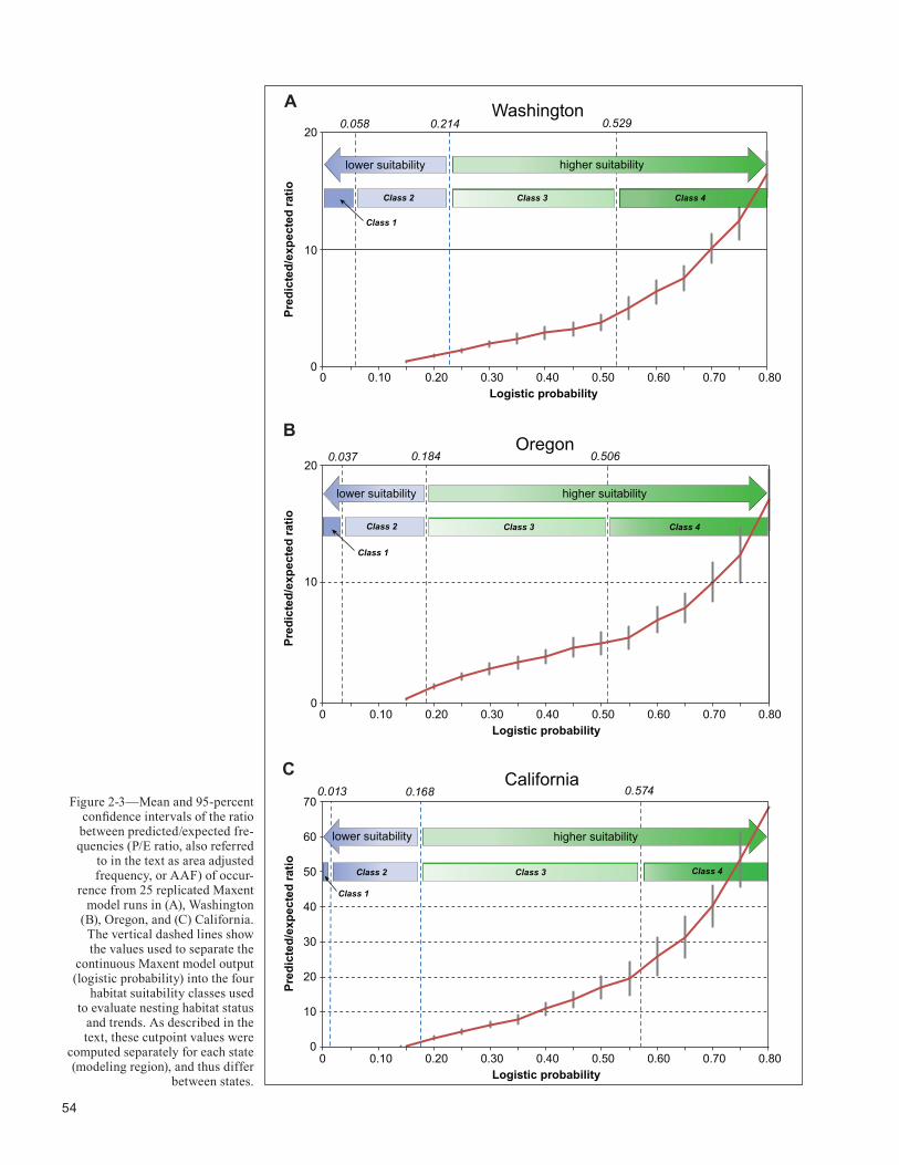
54
GENERAL TECHNICAL REPORT PNW-GTR-933
Figure 2-3—Mean and 95-percent confidence intervals of the ratio between predicted/expected fre-quencies (P/E ratio, also referred
to in the text as area adjusted frequency, or AAF) of occur-
rence from 25 replicated Maxent model runs in (A), Washington
(B), Oregon, and (C) California. The vertical dashed lines show the values used to separate the
continuous Maxent model output (logistic probability) into the four
habitat suitability classes used to evaluate nesting habitat status
and trends. As described in the text, these cutpoint values were
computed separately for each state (modeling region), and thus differ
between states.
0
10
20
0 0.10 0.20 0.30 0.40 0.50 0.60 0.70 0.80
Pred
icte
d/ex
pect
ed ra
tio
Logistic probability
Washington
lower suitability
Class 3 Class 4 Class 2
0.058 0.214 0.529
Class 2
0.037 0.184 0.506
higher suitability
A
0
10
20
0 0.10 0.20 0.30 0.40 0.50 0.60 0.70 0.80
Pred
icte
d/ex
pect
ed ra
tio
Logistic probability
Oregon
lower suitability
Class 2
B
higher suitability
Class 1
Class 1
Class 3 Class 4
0.1680.013 0.57470
60
50
40
30
20
10
0
Pred
icte
d/ex
pect
ed ra
tio
0 0.10 0.20 0.30 0.40 0.50 0.60 0.70 0.80Logistic probability
CaliforniaC
lower suitability higher suitability
Class 3 Class 4 Class 2
Class 1

55
Status and Trend of Marbled Murrelet Populations and Nesting Habitat
• Class 1 (lowest suitability) includes all pixels with logistic probability values between (a) zero and (b) the mean logistic value for all pixels below the P/E = 1 threshold.
• Class 2 (marginal suitability) includes all pixels with logistic probability values between (a) the mean logistic value for all pixels below the P/E = 1 thresh-old, and (b) the P/E = 1 threshold.
• Class 3 (moderate suitability) includes all pixels with logistic probability values between (a) the P/E = 1 threshold and (b) the mean logistic score for all nest and occupied locations used for modeling in that state. One can also think of this category as including those pixels for which the relative like-lihood of murrelet presence exceeds that expected by chance, given the set of environmental condi-tions (covariate values) at that pixel, while exclud-ing those in the highest suitability Class 4.
• Class 4 (highest suitability) includes all pixels with logistic probability values between the mean logistic score for all nest and occupied locations used for modeling in that state, and the maximum score (gen-erally close to 1.0). Thus, this class included pixels with probability scores equal or exceeding the aver-age score of the presence (training) sites used in that state’s model. One can think of this class as approx-imating locations where environmental conditions equal to or exceeding those of the average nest/occu-pied location in our dataset.
After calculating the values used to classify the 1993 model output (logistic scores) for each state into these four classes, we applied those same values to the 2012 maps of habitat suitability (logistic scores) which had been created by projecting the 1993 models onto the 2012 covariate conditions. Therefore, for each state, the same models and thresholds were used to model habitat suitability and then to classify the resulting habitat suitability maps for both the 1993 baseline and the 2012 bookend.
To portray variability in our estimates of amounts of suitable nesting habitat, we computed the standard deviation and mean acres of higher suitability habitat (Classes 3 and 4 combined). To do this calculation, we obtained the 25 sets
of logistic probability maps from the 25 replicated Maxent runs, calculated acres above the threshold from each map, and then computed the mean and standard deviation of those acre values from the 25 replicate maps for each study region (state).
We tested for a change in nesting habitat area from 1993 to 2012 by running matched-pair t-tests on the estimates of higher suitability habitat at the scales of state, physiographic province, and main LUA class (nonfed-eral, federal reserved, federal nonreserved). We used a matched-pair approach because we wanted to control for variability among the 25 replicated model runs conducted for each state model. Each replicate was based on a model built on the 1993 environmental data and that same model was projected to the new 2012 environmental data, thus providing a matched pair consisting of 1993 and 2012 habitat estimates for each replicate. We used those matched estimates for each replicate to compute the difference in acres of higher suitability habitat from 1993 to 2012 for each replicate, and then computed the mean difference across all replicates to test the likelihood of observing those data under a null hypothesis of no difference in mean acres between time periods.
The plot of P/E against the mean habitat suitability of each class (fig. 2-3) provides a test for model performance, as a good model is expected to show a monotonically increasing curve (Boyce et al. 2002), for which we tested using the Spearman rank correlation coefficient (Boyce et al. 2002, Hirzel et al. 2006).
Landscape Habitat Pattern—Edge Versus CoreMarbled murrelet nest success is reduced along forested edges because of higher rates of nest depredation near edges (Malt and Lank 2007, Manley and Nelson 1999, Raphael et al. 2002). For that reason, we investigated the configuration of potential habitat by computing how much of that habitat occurred along edges versus within forest interior conditions. We used the morphometric spatial pattern analysis (MSPA) tool in the GUIDOS (Vogt 2013) toolbox to characterize murrelet nesting habitat configu-ration. The GUIDOS toolbox is a software program with functions for processing and visualizing spatial data.
56
GENERAL TECHNICAL REPORT PNW-GTR-933
MSPA is an algorithm that classifies pixels in a binary raster image based on their geometry and connectivity to other pixels. Contiguous clusters of habitat pixels are considered a patch. Each patch has a zone of ‘edge’ habitat along its periphery, defined by the ‘edge depth’ parameter. In the middle of the patch, inside of the edge zone, pixels are classified as ‘core’ habitat. MSPA may optionally further classify certain edge pixels based on their configu-ration in areas of transition between core and edge. These transitional classes include ‘islets’ (edge pixels in patches too small to contain core habitat), ‘bridges’ (edge pixels that link separate patches of core habitat),‘loops’ (edge pixels that connect lobes within a core habitat patch, ‘per-forations’ (the edge of a non-habitat patch contained within a habitat patch), and ‘branches’ (narrow protrusions of edge habitat extending outwards from patches of core habitat). In addition, MSPA allows edge classes to be further classified as combinations of the above subtypes (e.g., ‘loop in edge,’ or ‘bridge in perforation’).
We performed MSPA based on the maps of higher suit-ability nesting habitat (Classes 3 plus 4) identified for each state, for both 1993 and 2012. MSPA parameters included an edge depth of 90 m, an 8-cell connection rule (i.e., diagonal connections were allowed when assigning pixels to habitat patches), transitions were enabled (i.e., transitional classes were allowed), and ‘intext’ was enabled (i.e., combinations of edge classes were allowed). Classification using these settings produced 11 MSPA classes, which we aggregated into 3 classes, including:• Core (only includes ‘core’ MSPA class). This class
represents core higher suitability habitat that is fur-ther than 90 m from an edge.
• Core-edge (including MSPA classes ‘islet’, ‘loop’, ‘bridge’, and ‘branch’). This class represents edges of higher suitability habitat within 90 m of core habitat.
• Edge (including MSPA classes ‘perforation’, ‘edge’, ‘loop in edge’, ‘loop in perforation’, ‘bridge in edge’, and ‘bridge in perforation’). This class includes nar-row ribbons of edge higher suitability habitat which occur more than 90 m beyond core pixels, or isolated patches too small or narrow to contain core pixels.
Human DisturbanceMarbled murrelet nest site selection is thought to be sensitive to human modification of the landscape. We quantified human landscape modification based on a “human footprint” model (Leu et al. 2008) of anthropo-genic impacts in the Western United States. This model considers human habitation, roads, railroads, irrigation canals, power lines, linear feature densities, agricultural land, campgrounds, highway rest stops, landfills, oil and gas development, and human-induced fires. These impacts were summarized spatially in a raster model with values corresponding to 10 human footprint ranks, with a value of 1 being the least modification and 10 the greatest. To assess the amount of potential nesting habitat poten-tially degraded by these human impacts, we calculated the acres of nesting habitat within each of the 10 ranks, summarized by state and bookend year. In addition, to determine if the degree of human modification of the landscape differed between suitable core and edge habitats, we calculated the mean human footprint rank of habitat pixels in each landscape pattern class (core, core-edge, and edge).
ResultsCovariatesMean values of each covariate differed between training sites and study region (table 2-3). Maxent output includes estimates of the relative contribution of each covariate to the final model (table 2-4). These values are estimated by Maxent during the iterative model optimization process, and are based on the increase in training gain associated with each covariate. The contribution values should be interpreted with caution for covariates that are highly correlated. This is because there is an element of chance in how the percentage of contribution is divided among highly correlated covariates; one of a pair of such covar-iates may be assigned a high contribution and the other a low contribution when in fact both may be important to the species (Phillips n.d.). As described earlier, we included correlated variables in models because our intent was to use the available data to produce the strongest predictive accuracy of habitat suitability.
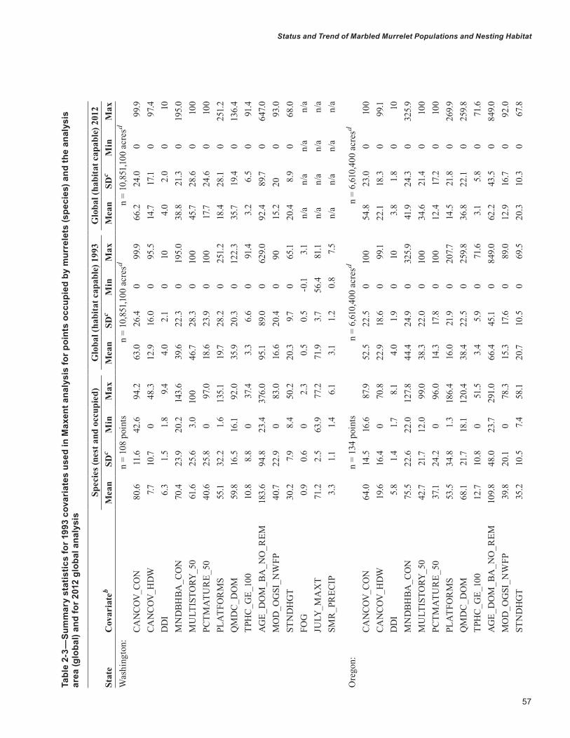
57
Status and Trend of Marbled Murrelet Populations and Nesting Habitat
Tabl
e 2-
3—Su
mm
ary
stat
istic
s fo
r 199
3 co
vari
ates
use
d in
Max
ent a
naly
sis
for p
oint
s oc
cupi
ed b
y m
urre
lets
(spe
cies
) and
the
anal
ysis
ar
ea (g
loba
l) an
d fo
r 201
2 gl
obal
ana
lysi
s
Stat
eC
ovar
iate
bSp
ecie
s (ne
st a
nd o
ccup
ied)
Glo
bal (
habi
tat c
apab
le) 1
993
Glo
bal (
habi
tat c
apab
le) 2
012
Mea
nSD
cM
inM
axM
ean
SDc
Min
Max
Mea
nSD
cM
inM
axW
ashi
ngto
n:n
= 10
8 po
ints
n =
10,8
51,10
0 ac
resd
n =
10,8
51,10
0 ac
resd
CAN
CO
V_C
ON
80.6
11.6
42.6
94.2
63.0
26.4
099
.966
.224
.00
99.9
CAN
CO
V_H
DW
7.710
.70
48.3
12.9
16.0
095
.514
.717
.10
97.4
DD
I6.
31.
51.
89.
44.
02.
10
104.
02.
00
10M
ND
BHBA
_CO
N70
.423
.920
.214
3.6
39.6
22.3
019
5.0
38.8
21.3
019
5.0
MU
LTIS
TORY
_50
61.6
25.6
3.0
100
46.7
28.3
010
045
.728
.60
100
PCTM
ATU
RE_
5040
.625
.80
97.0
18.6
23.9
010
017
.724
.60
100
PLA
TFO
RM
S55
.132
.21.
613
5.1
19.7
28.2
025
1.2
18.4
28.1
025
1.2
QM
DC
_DO
M59
.816
.516
.192
.035
.920
.30
122.
335
.719
.40
136.
4TP
HC
_GE_
100
10.8
8.8
037
.43.
36.
60
91.4
3.2
6.5
091
.4A
GE_
DO
M_B
A_N
O_R
EM18
3.6
94.8
23.4
376.
095
.189
.00
629.
092
.489
.70
647.
0M
OD
_OG
SI_N
WFP
40.7
22.9
083
.016
.620
.40
9015
.220
093
.0ST
ND
HG
T30
.27.
98.
450
.220
.39.7
065
.120
.48.
90
68.0
FOG
0.9
0.6
02.
30.
50.
5-0
.13.
1n/
an/
an/
an/
aJU
LY_M
AX
T71
.22.
563
.977
.271
.93.
756
.481
.1n/
an/
an/
an/
aSM
R_P
REC
IP3.
31.1
1.4
6.1
3.1
1.2
0.8
7.5
n/a
n/a
n/a
n/a
Ore
gon:
n =
134
poin
tsn
= 6,
610,
400
acre
sdn
= 6,
610,
400
acre
sd
CAN
CO
V_C
ON
64.0
14.5
16.6
87.9
52.5
22.5
010
054
.823
.00
100
CAN
CO
V_H
DW
19.6
16.4
070
.822
.918
.60
99.1
22.1
18.3
099
.1D
DI
5.8
1.4
1.78.
14.
01.
90
103.
81.
80
10M
ND
BHBA
_CO
N75
.522
.622
.012
7.8
44.4
24.9
032
5.9
41.9
24.3
032
5.9
MU
LTIS
TORY
_50
42.7
21.7
12.0
99.0
38.3
22.0
010
034
.621
.40
100
PCTM
ATU
RE_
5037
.124
.20
96.0
14.3
17.8
010
012
.417
.20
100
PLA
TFO
RM
S53
.534
.81.
318
6.4
16.0
21.9
020
7.714
.521
.80
269.
9Q
MD
C_D
OM
68.1
21.7
18.1
120.
438
.422
.50
259.
836
.822
.10
259.
8TP
HC
_GE_
100
12.7
10.8
051
.53.
45.
90
71.6
3.1
5.8
071
.6A
GE_
DO
M_B
A_N
O_R
EM10
9.8
48.0
23.7
291.
066
.445
.10
849.
062
.243
.50
849.
0M
OD
_OG
SI_N
WFP
39.8
20.1
078
.315
.317
.60
89.0
12.9
16.7
092
.0ST
ND
HG
T35
.210
.57.
458
.120
.710
.50
69.5
20.3
10.3
067
.8

58
GENERAL TECHNICAL REPORT PNW-GTR-933
Stat
eC
ovar
iate
bSp
ecie
s (ne
st a
nd o
ccup
ied)
Glo
bal (
habi
tat c
apab
le) 1
993
Glo
bal (
habi
tat c
apab
le) 2
012
Mea
nSD
cM
inM
axM
ean
SDc
Min
Max
Mea
nSD
cM
inM
axFO
G0.
50.
40.
12.
00.
40.
50
2.9
n/a
n/a
n/a
n/a
JULY
_MA
XT
75.1
3.9
64.2
85.6
76.4
4.9
58.0
91.9
n/a
n/a
n/a
n/a
SMR
_PR
ECIP
2.7
0.7
1.14.
32.
20.
80.
95.
7n/
an/
an/
an/
a
Cal
iforn
ia:
n =
126
poin
tsn
= 3,
250,
100
acre
sdn
= 3,
250,
100
acre
sd
CAN
CO
V_C
ON
84.6
15.4
15.1
99.5
51.0
22.9
010
054
.022
.50
100
CAN
CO
V_H
DW
26.8
20.7
075
.844
.622
.70
97.5
45.4
22.7
097
.8D
DI
6.7
1.4
2.2
9.6
4.8
1.6
010
4.9
1.5
010
MN
DBH
BA_C
ON
110.
249
.614
.829
0.3
52.6
27.7
032
5.9
53.3
26.5
032
5.9
MU
LTIS
TORY
_50
73.1
19.9
18.0
100
64.8
23.0
010
068
.322
.90
100
PCTM
ATU
RE_
5042
.726
.70
98.0
10.4
16.5
010
010
.216
.10
100
PLA
TFO
RM
S82
.863
.60.
222
1.0
16.0
24.8
022
1.0
16.0
23.8
022
1.0
QM
DC
_DO
M84
.635
.513
.623
1.2
43.5
23.5
025
9.8
43.8
22.3
025
9.8
TPH
C_G
E_10
024
.118
.10
61.7
4.2
7.5
071
.64.
17.
20
71.6
AG
E_D
OM
_BA
_NO
_REM
181.
510
9.144
.972
8.3
85.4
58.2
084
9.0
83.9
56.0
084
9.0
MO
D_O
GSI
_NW
FP49
.124
.63.
688
.020
.918
.00
88.0
20.5
17.0
088
.0ST
ND
HG
T33
.110
.68.
762
.818
.47.
50
67.8
18.8
7.10
67.8
FOG
1.2
0.1
0.9
1.5
1.0
0.4
0.1
1.8
n/a
n/a
n/a
n/a
JULY
_MA
XT
74.0
4.7
65.1
85.6
80.7
7.157
.699
.0n/
an/
an/
an/
aSM
R_P
REC
IP1.1
0.3
0.5
2.0
1.4
0.7
0.3
4.1
n/a
n/a
n/a
n/a
a Max
ent i
s a h
abita
t-sui
tabi
lity
mod
elin
g so
ftw
are
used
in th
is st
udy
to m
odel
rela
tive
suita
bilit
y of
mar
bled
mur
rele
t nes
ting
habi
tat.
b Des
crip
tion
of th
e co
varia
tes,
incl
udin
g un
its, c
an b
e fo
und
in ta
ble
2-1.
c Stan
dard
dev
iatio
n.d
Rep
rese
nts a
naly
sis a
rea
in m
arbl
ed m
urre
let N
WFP
Inla
nd Z
ones
1 a
nd 2
in W
ashi
ngto
n an
d In
land
Zon
e 1
only
in O
rego
n an
d C
alifo
rnia
. Fig
ures
are
roun
ded
to th
e ne
ares
t 100
acr
es.
Tabl
e 2-
3—Su
mm
ary
stat
istic
s fo
r 199
3 co
vari
ates
use
d in
Max
ent a
naly
sis
for p
oint
s oc
cupi
ed b
y m
urre
lets
(spe
cies
) and
the
anal
ysis
ar
ea (g
loba
l) an
d fo
r 201
2 gl
obal
ana
lysi
s (c
ontin
ued)
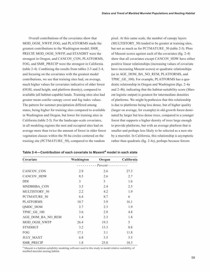
59
Status and Trend of Marbled Murrelet Populations and Nesting Habitat
Overall contributions of the covariates show that MOD_OGSI_NWFP, FOG, and PLATFORMS made the greatest contributions to the Washington model; SMR_PRECIP, MOD_OGSI_NWFP, and STANDHT were the strongest in Oregon, and CANCOV_CON, PLATFORMS, FOG, and SMR_PRECIP were the strongest in California (table 2-4). Combining the results from tables 2-3 and 2-4, and focusing on the covariates with the greatest model contributions, we see that training sites had, on average, much higher values for covariates indicative of older forest (OGSI, stand height, and platform density), compared to available (all habitat-capable) lands. Training sites also had greater mean conifer canopy cover and fog index values. The pattern for summer precipitation differed among states, being higher for training sites compared to available in Washington and Oregon, but lower for training sites in California (table 2-3). For the landscape-scale covariates, in all modeling regions the nest and occupied sites had on average more than twice the amount of forest in older forest vegetation classes within the 50-ha circles centered on the training site (PCTMATURE_50), compared to the random
pixel. At this same scale, the number of canopy layers (MULTISTORY_50) tended to be greater at training sites, but not as much as for PCTMATURE_50 (table 2-3). Plots of Maxent scores against each of the covariates (fig. 2-4) show that all covariates except CANCOV_HDW have either positive linear relationships (increasing values of covariate have increasing Maxent scores) or quadratic relationships (as in AGE_DOM_BA_NO_REM, PLATFORMS, and TPHC_GE_100). For example, PLATFORMS has a qua-dratic relationship in Oregon and Washington (figs. 2-4a and 2-4b), indicating that the habitat-suitability score (Max-ent logistic output) is greatest for intermediate densities of platforms. We might hypothesize that this relationship is due to platforms being less dense, but of higher quality (larger on average, for example) in old-growth forest domi-nated by larger but less dense trees, compared to a younger forest that supports a higher density of trees large enough to provide platforms, but with an average platform that is smaller and perhaps less likely to be selected as a nest site by a murrelet. In California, this relationship is asymptotic rather than quadratic (fig. 2-4c), perhaps because forests
Table 2-4—Contribution of each covariate to Maxenta model in each state
Covariate Washington Oregon California
- - - - - - - - - - Percent - - - - - - - - - -
CANCOV_CON 2.9 2.6 27.3CANCOV_HDW 8.5 2.6 2.7DDI 3 3 1.6MNDBHBA_CON 3.5 2.4 2.5MULTISTORY_50 2.2 4.2 1.9PCTMATURE_50 6.4 8.7 6PLATFORMS 10.7 3.9 16.1QMDC_DOM 2.7 2.3 1.9TPHC_GE_100 3.6 2.9 4.8AGE_DOM_BA_NO_REM 1.4 2.3 1.8MOD_OGSI_NWFP 26.4 19.3 5STNDHGT 3.2 13.3 0.8FOG 17.1 3.1 11.8JULY_MAXT 6.8 3.5 5.5SMR_PRECIP 1.8 25.8 10.3a Maxent is a habitat-suitability modeling software used in this study to model relative suitability of marbled murrelet nesting habitat.

60
GENERAL TECHNICAL REPORT PNW-GTR-933
Figure 2-4—Response curves showing how each variable affects the habitat-suitability score in (A) Washington, (B) Oregon, and (C) California. The red lines indicate mean response across 25 replicated model runs; blue shapes represent 1 standard deviation above and below the mean. The curves show in relative terms how the habitat-suitability changes across the range of covariate values (horizontal axis) found within the modeling region, whereas all other covariates are kept at their average value in the modeling region.
A
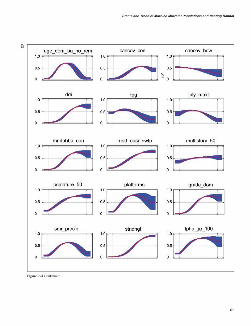
61
Status and Trend of Marbled Murrelet Populations and Nesting Habitat
Figure 2-4 Continued.
B

62
GENERAL TECHNICAL REPORT PNW-GTR-933
Figure 2-4 Continued.
C
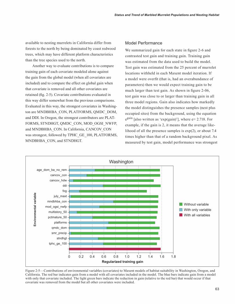
63
Status and Trend of Marbled Murrelet Populations and Nesting Habitat
age_dom_ba_no_rem
cancov_con
cancov_hdw
ddi
fog
july_maxt
mndbhba_con
mod_ogsi_nwfp
multistory_50
pctmature_50
platforms
qmdc_dom
smr_precip
stndhgt
tphc_ge_100
Envi
ronm
enta
l var
iabl
e
0 0.2 0.4 0.6 0.8 1.0 1.2 1.4 1.6 1.8Regularized training gain
Washington
Without variableWith only variableWith all variables
Figure 2-5—Contributions of environmental variables (covariates) to Maxent models of habitat suitability in Washington, Oregon, and California. The red bar indicates gain from a model with all covariates included in the model. The blue bars indicate gain from a model with only that covariate included. The light green bars indicate the reduction in gain (relative to the red bar) that would occur if that covariate was removed from the model but all other covariates were included.
available to nesting murrelets in California differ from forests to the north by being dominated by coast redwood trees, which may have different platform characteristics than the tree species used to the north.
Another way to evaluate contributions is to compare training gain of each covariate modeled alone against the gain from the global model (when all covariates are included) and to compare the effect on global gain when that covariate is removed and all other covariates are retained (fig. 2-5). Covariate contributions evaluated in this way differ somewhat from the previous comparisons. Evaluated in this way, the strongest covariates in Washing-ton are MNDBHBA_CON, PLATFORMS, QMDC_DOM, and DDI. In Oregon, the strongest contributors are PLAT-FORMS, STNDHGT, QMDC_CON, MOD_OGSI_NWFP, and MNDBHBA_CON. In California, CANCOV_CON was strongest, followed by TPHC_GE_100, PLATFORMS, MNDBHBA_CON, and STNDHGT.
Model PerformanceWe summarized gain for each state in figure 2-6 and contrasted test gain and training gain. Training gain was estimated from the data used to build the model. Test gain was estimated from the 25 percent of murrelet locations withheld in each Maxent model iteration. If a model were overfit (that is, had an overabundance of parameters) then we would expect training gain to be much larger than test gain. As shown in figure 2-06, test gain was close to or larger than training gain in all three model regions. Gain also indicates how markedly the model distinguishes the presence samples (nest plus occupied sites) from the background, using the equation egain [also written as ‘exp(gain)’], where e≈ 2.718. For example, if the gain is 2, it means that the average like-lihood of all the presence samples is exp(2), or about 7.4 times higher than that of a random background pixel. As measured by test gain, model performance was strongest
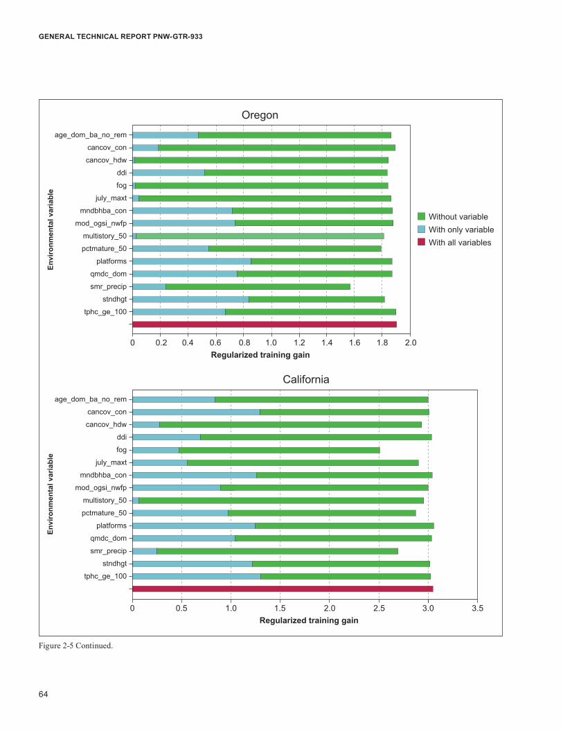
64
GENERAL TECHNICAL REPORT PNW-GTR-933
Figure 2-5 Continued.
Envi
ronm
enta
l var
iabl
e
0 0.2 0.4 0.6 0.8 1.0 1.2 1.4 1.6 1.8 2.0Regularized training gain
Oregon
Envi
ronm
enta
l var
iabl
e
0 0.5 1.0 1.5 2.0 2.5 3.0 3.5Regularized training gain
California
Without variableWith only variableWith all variables
age_dom_ba_no_rem
cancov_con
cancov_hdw
ddi
fog
july_maxt
mndbhba_con
mod_ogsi_nwfp
multistory_50
pctmature_50
platforms
qmdc_dom
smr_precip
stndhgt
tphc_ge_100
age_dom_ba_no_rem
cancov_con
cancov_hdw
ddi
fog
july_maxt
mndbhba_con
mod_ogsi_nwfp
multistory_50
pctmature_50
platforms
qmdc_dom
smr_precip
stndhgt
tphc_ge_100

65
Status and Trend of Marbled Murrelet Populations and Nesting Habitat
in California [gain = 3.065, and exp(3.065) = 21.4], indicating a much stronger distinction between murrelet sites and the background area in that state compared with the other states. Test gains were lower in Oregon (gain = 1.634, exp(1.634) = 5.1) and Washington (gain = 1.469, exp(1.469) = 4.34). In all states, test gains were higher than in the NWFP 15-year analysis (Washington: 1.092, Oregon 1.041, California 2.976) (Raphael et al. 2011).
Test AUC values were ranked among the model regions in the same pattern as gain: AUC was greatest in the California model (AUC = 0.960) and lower in the models for Oregon (AUC = 0.892) and Washington (AUC = 0.874) (fig. 2-6). For all three models, the plot of P/E values against the mean habitat suitability of each class showed a monotonically increasing curve with high correlation value (Rs > 0.99; P < 0.001), indicative of strong model perfor-mance (fig. 2-3).
Habitat SuitabilityOur models estimated the suitability of conditions for murrelet occurrence at two points in time: the start of the NWFP (1993) and current (2012) (tables 2-5 through 2-8 and figs. 2-7 through 2-13). As summarized in figure 2-12, most land is classified in the lower suitability Classes 1 and 2, with successively fewer acres in the higher classes above our suitability threshold. The proportion of habi-tat-capable land that was above the threshold (in Classes 3 plus 4) at the start of the NWFP varied among model regions (states) and land ownerships. In Washington, 14.3 percent of all habitat-capable land was classified above the threshold in 1993; in Oregon and California 12.9 and 4.1 percent, respectively, were above the threshold in 1993 (table 2-8). The proportion in suitable classes was greater on federal lands than nonfederal in Washington (25.9 percent versus 8.8 percent) and Oregon (23.4 percent versus 6.7 percent), but lower in California (2.7 percent versus 4.7 percent), where relatively little habitat-capable area occurs on federal land (tables 2-5 through 2-8). Over all lands, we estimated a total of 2.53 million ac of higher suitability habitat in 1993 (12.2 percent of habitat-capable land; see table 2-8). Most of this nesting habitat (54 percent) was on federally reserved lands, but
Figure 2-6—Model performance and thresholds by model region (state), with 95-percent confidence intervals. See text for expla-nations of performance metrics. AUC = area under the curve statistics P/E = predicted/expected.
California
Regularizedtraining
gain
Testgain
TestAUC
P/E = 13.056 3.065 0.960 0.168
3.5
3.0
2.5
2.0
1.5
1.0
0.5
0
Regularizedtraining
gain
Testgain
TestAUC
P/E = 11.907 1.634 0.892 0.1840
Oregon2.5
2.0
1.5
1.0
0.5
0
0.2
0.4
0.6
0.8
1.0
1.2
1.4
1.6
1.8
Regularizedtraining
gain
Testgain
TestAUC
P/E = 1
Washington
1.586 1.469 0.874 0.214
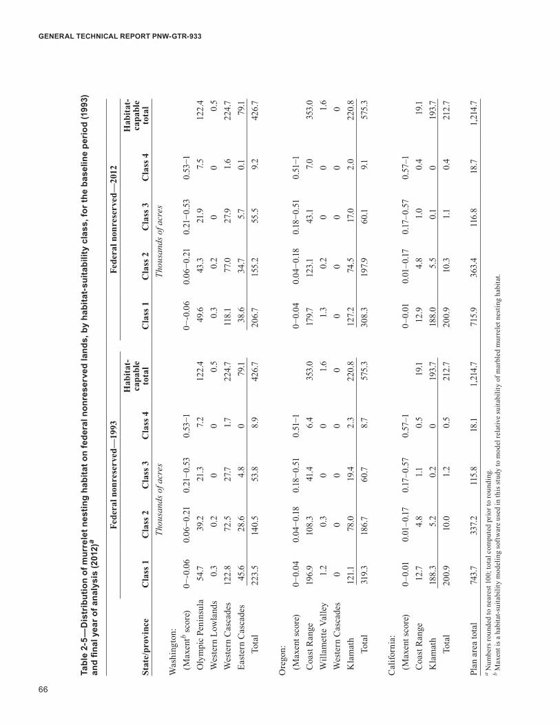
66
GENERAL TECHNICAL REPORT PNW-GTR-933
Tabl
e 2-
5—D
istr
ibut
ion
of m
urre
let n
estin
g ha
bita
t on
fede
ral n
onre
serv
ed la
nds,
by
habi
tat-
suita
bilit
y cl
ass,
for t
he b
asel
ine
peri
od (1
993)
an
d fin
al y
ear o
f ana
lysi
s (2
012)
a
Fede
ral n
onre
serv
ed—
1993
Fe
dera
l non
rese
rved
—20
12
Stat
e/pr
ovin
ceC
lass
1C
lass
2C
lass
3C
lass
4
Hab
itat-
capa
ble
tota
lC
lass
1C
lass
2C
lass
3C
lass
4
Hab
itat-
capa
ble
tota
lTh
ousa
nds o
f acr
esTh
ousa
nds o
f acr
esW
ashi
ngto
n:(M
axen
tb scor
e)0−
-0.0
60.
06−0
.21
0.21
−0.5
30.
53−1
0−-0
.06
0.06
−0.2
10.
21−0
.53
0.53
−1O
lym
pic
Peni
nsul
a54
.739
.221
.37.
212
2.4
49.6
43.3
21.9
7.5
122.
4W
este
rn L
owla
nds
0.3
0.2
00
0.5
0.3
0.2
00
0.5
Wes
tern
Cas
cade
s 12
2.8
72.5
27.7
1.722
4.7
118.
177
.027
.91.
622
4.7
East
ern
Cas
cade
s 45
.628
.64.
80
79.1
38.6
34.7
5.7
0.1
79.1
Tota
l22
3.5
140.
553
.88.
942
6.7
206.
715
5.2
55.5
9.2
426.
7
Ore
gon:
(Max
ent s
core
)0−
0.04
0.04
−0.18
0.18
−0.5
10.
51−1
0−0.
040.
04−0
.180.
18−0
.51
0.51
−1C
oast
Ran
ge19
6.9
108.
341
.46.
435
3.0
179.7
123.
143
.17.
035
3.0
Will
amet
te V
alle
y1.
20.
30
01.
61.
30.
20
01.
6W
este
rn C
asca
des
00
00
00
00
00
Kla
mat
h12
1.178
.019
.42.
322
0.8
127.
274
.517
.02.
022
0.8
Tota
l31
9.3
186.
760
.78.
757
5.3
308.
319
7.9
60.1
9.157
5.3
Cal
iforn
ia:
(Max
ent s
core
)0–
0.01
0.01
–0.17
0.17
–0.5
70.
57–1
0–0.
010.
01–0
.170.
17–0
.57
0.57
–1C
oast
Ran
ge12
.74.
81.1
0.5
19.1
12.9
4.8
1.0
0.4
19.1
Kla
mat
h18
8.3
5.2
0.2
019
3.7
188.
05.
50.
10
193.
7To
tal
200.
910
.01.
20.
521
2.7
200.
910
.31.1
0.4
212.
7
Pl
an a
rea
tota
l74
3.7
337.
211
5.8
18.1
1,21
4.7
715.
936
3.4
116.
818
.71,
214.
7a N
umbe
rs ro
unde
d to
nea
rest
100
; tot
al c
ompu
ted
prio
r to
roun
ding
. b M
axen
t is a
hab
itat-s
uita
bilit
y m
odel
ing
soft
war
e us
ed in
this
stud
y to
mod
el re
lativ
e su
itabi
lity
of m
arbl
ed m
urre
let n
estin
g ha
bita
t.
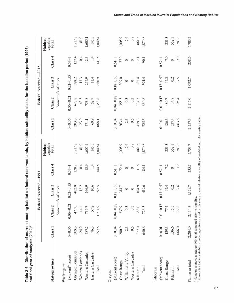
67
Status and Trend of Marbled Murrelet Populations and Nesting Habitat
Tabl
e 2-
6—D
istr
ibut
ion
of m
urre
let n
estin
g ha
bita
t on
fede
ral r
eser
ved
land
s, b
y ha
bita
t-su
itabi
lity
clas
s, fo
r the
bas
elin
e pe
riod
(199
3)
and
final
yea
r of a
naly
sis
(201
2)a
Fede
ral r
eser
ved—
1993
Fede
ral r
eser
ved—
2012
Stat
e/pr
ovin
ceC
lass
1C
lass
2C
lass
3C
lass
4
Hab
itat-
capa
ble
tota
lC
lass
1C
lass
2C
lass
3C
lass
4
Hab
itat-
capa
ble
tota
lTh
ousa
nds o
f acr
esTh
ousa
nds o
f acr
esW
ashi
ngto
n:(M
axen
tb scor
e)0−
0.06
0.06
−0.2
10.
21−0
.53
0.53
−10−
0.06
0.06
−0.2
10.
21−0
.53
0.53
−1O
lym
pic
Peni
nsul
a20
9.3
477.
040
2.8
128.
71,
217.
820
3.3
498.
838
8.2
127.
41,
217.
8W
este
rn L
owla
nds
24.2
44.1
12.2
0.4
81.0
23.9
43.5
13.3
0.4
81.0
Wes
tern
Cas
cade
s 58
7.773
6.7
266.
913
.91,
605.
157
1.175
3.8
267.
912
.31,
605.
1Ea
ster
n C
asca
des
76.3
57.2
10.6
1.4
145.
569
.962
.711
.41.
414
5.5
Tota
l89
7.5
1,31
4.9
692.
514
4.5
3,04
9.4
868.
11,
358.
868
0.9
141.
53,
049.
4
Ore
gon:
(Max
ent s
core
)0−
0.04
0.04
−0.18
0.18
−0.5
10.
51−1
0−0.
040.
04−0
.180.
18−0
.51
0.51
−1C
oast
Ran
ge28
0.9
337.
931
4.7
72.4
1,00
5.9
263.
435
5.5
309.
077
.91,
005.
9W
illam
ette
Val
ley
2.3
0.3
00
2.6
2.3
0.3
00
2.6
Wes
tern
Cas
cade
s0.
50.
30
00.
80.
50.
30
00.
8K
lam
ath
357.
038
8.0
104.
911
.686
1.5
459.
330
4.7
85.4
12.1
861.
5To
tal
640.
672
6.5
419.
684
.11,
870.
872
5.5
660.
839
4.4
90.1
1,87
0.8
Cal
iforn
ia:
(Max
ent s
core
)0−
0.01
0.01
−0.17
0.17
−0.5
70.
57−1
0−0
.01
0.01
−0.17
0.17
−0.5
70.
57−1
Coa
st R
ange
129.
377
.417
.47.
223
1.3
126.
380
.717
.37.
023
1.3
Kla
mat
h53
6.6
15.5
0.2
055
2.3
537.
414
.80.
20
552.
3To
tal
666.
092
.817
.67.
278
3.6
663.
695
.417
.57.
078
3.6
Plan
are
a to
tal
2,20
4.0
2,13
4.3
1,12
9.723
5.7
5,70
3.7
2,25
7.3
2,11
5.0
1,09
2.7
238.
65,
703.
7a N
umbe
rs ro
unde
d to
nea
rest
100
; tot
al c
ompu
ted
prio
r to
roun
ding
. b M
axen
t is a
hab
itat s
uita
bilit
y m
odel
ing
soft
war
e us
ed in
this
stud
y to
mod
el re
lativ
e su
itabi
lity
of m
arbl
ed m
urre
let n
estin
g ha
bita
t.
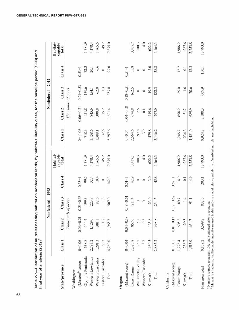
68
GENERAL TECHNICAL REPORT PNW-GTR-933
Tabl
e 2-
7—D
istr
ibut
ion
of m
urre
let n
estin
g ha
bita
t on
nonf
eder
al la
nds,
by
habi
tat-
suita
bilit
y cl
ass,
for t
he b
asel
ine
peri
od (1
993)
and
fin
al y
ear o
f ana
lysi
s (2
012)
a
Non
fede
ral—
1993
Non
fede
ral—
2012
Stat
e/pr
ovin
ceC
lass
1C
lass
2C
lass
3C
lass
4
Hab
itat-
capa
ble
tota
lC
lass
1C
lass
2C
lass
3C
lass
4
Hab
itat-
capa
ble
tota
lTh
ousa
nds o
f acr
esTh
ousa
nds o
f acr
esW
ashi
ngto
n:(M
axen
tb scor
e)0−
0.06
0.06
−0.2
10.
21−0
.53
0.53
−10−
-0.0
60.
06−0
.21
0.21
−0.5
30.
53−1
Oly
mpi
c Pe
nins
ula
638.
844
4.4
199.
399
.51,
381.
971
8.3
451.
813
9.6
72.3
1,38
1.9
Wes
tern
Low
land
s 2,
793.
21,
129.
022
3.8
32.4
4,17
8.4
3,15
8.6
845.
615
4.1
20.1
4,17
8.4
Wes
tern
Cas
cade
s 1,
291.
338
1.182
.610
.41,7
65.5
1,38
8.1
308.
862
.06.
61,7
65.5
East
ern
Cas
cade
s 36
.711
.21.
30
49.2
32.6
15.2
1.3
049
.2To
tal
4,76
0.0
1,96
5.7
507.
014
2.3
7,37
5.0
5,29
7.6
1,62
1.4
357.
099
.07,
375.
0
Ore
gon:
(Max
ent s
core
)0−
0.04
0.04
−0.18
0.18
−0.5
10.
51−1
0−0.
040.
04−0
.180.
18−0
.51
0.51
−1C
oast
Ran
ge2,
325.
885
7.6
211.
442
.93,
437.7
2,56
4.6
674.
816
2.5
35.8
3,43
7.7W
illam
ette
Val
ley
95.2
5.1
00
100.
397
.82.
50
010
0.3
Wes
tern
Cas
cade
s3.
70.
30
04.
03.
90.
10
04.
0K
lam
ath
460.
513
5.8
23.0
3.0
622.
247
9.8
119.
619
.93.
062
2.2
Tota
l2,
885.
299
8.8
234.
545
.84,
164.
33,
146.
279
7.0
182.
338
.84,
164.
3
Cal
iforn
ia:
(Max
ent s
core
)0−
0.01
0.01
−0.17
0.17
−0.5
70.
57−1
Coa
st R
ange
1,27
6.4
605.
389
.714
.91,
986.
21,
246.
765
8.2
69.0
12.2
1,98
6.2
Kla
mat
h23
6.7
29.5
1.4
0.1
267.
623
4.3
31.7
1.6
0.1
267.
6To
tal
1,51
3.0
634.
791
.114
.92,
253.
81,
481.
068
9.9
70.6
12.3
2,25
3.8
Plan
are
a to
tal
9,15
8.2
3,59
9.2
832.
520
3.1
13,7
93.0
9,92
4.7
3,10
8.3
609.
915
0.1
13,7
93.0
a Num
bers
roun
ded
to n
eare
st 1
00; t
otal
com
pute
d pr
ior t
o ro
undi
ng.
b Max
ent i
s a h
abita
t-sui
tabi
lity
mod
elin
g so
ftw
are
used
in th
is st
udy
to m
odel
rela
tive
suita
bilit
y of
mar
bled
mur
rele
t nes
ting
habi
tat.
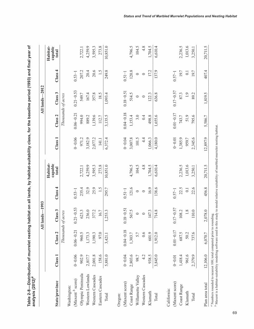
69
Status and Trend of Marbled Murrelet Populations and Nesting Habitat
Tabl
e 2-
8—D
istr
ibut
ion
of m
urre
let n
estin
g ha
bita
t on
all l
ands
, by
habi
tat-
suita
bilit
y cl
ass,
for t
he b
asel
ine
peri
od (1
993)
and
fina
l yea
r of
anal
ysis
(201
2)a
All
land
s—19
93A
ll la
nds—
2012
Stat
e/pr
ovin
ceC
lass
1C
lass
2C
lass
3C
lass
4
Hab
itat-
capa
ble
tota
lC
lass
1C
lass
2C
lass
3C
lass
4
Hab
itat-
capa
ble
tota
lTh
ousa
nds o
f acr
esTh
ousa
nds o
f acr
esW
ashi
ngto
n:(M
axen
t b scor
e)0−
0.06
0.06
−0.2
10.
21−0
.53
0.53
−10−
0.06
0.06
−0.2
10.
21−0
.53
0.53
−1 O
lym
pic
Peni
nsul
a90
2.9
960.
562
3.3
235.
42,
722.
197
1.2
994.
054
9.720
7.2
2,72
2.1
Wes
tern
Low
land
s 2,
817.7
1,17
3.3
236.
032
.94,
259.
93,
182.
988
9.2
167.
420
.44,
259.
9 W
este
rn C
asca
des
2,00
1.8
1,19
0.3
377.
225
.93,
595.
32,
077.
21,
139.
635
7.8
20.6
3,59
5.3
Eas
tern
Cas
cade
s 15
8.6
97.0
16.7
1.5
273.
814
1.111
2.7
18.5
1.5
273.
8
Tot
al5,
881.
03,
421.1
1,25
3.3
295.
710
,851
.06,
372.
43,
135.
51,
093.
424
9.8
10,8
51.0
Ore
gon:
(Max
ent s
core
)0−
0.04
0.04
−0.18
0.18
−0.5
10.
51−1
0−0.
040.
04−0
.180.
18−0
.51
0.51
−1 C
oast
Ran
ge2,
803.
61,
303.
756
7.5
121.
64,
796.
53,
007.
81,
153.
451
4.5
120.
84,
796.
5 W
illam
ette
Val
ley
98.7
5.7
00
104.
510
1.5
3.0
00
104.
5 W
este
rn C
asca
des
4.2
0.6
00
4.8
4.4
0.4
00
4.8
Kla
mat
h93
8.5
601.
914
7.3
16.9
1,704
.51,
066.
349
8.8
122.
317
.21,7
04.5
T
otal
3,84
5.0
1,91
2.0
714.
813
8.6
6,61
0.4
4,18
0.0
1,65
5.6
636.
813
7.9
6,61
0.4
Cal
iforn
ia:
(Max
ent s
core
)0−
0.01
0.01
−0.17
0.17
−0.5
70.
57−1
0−0
.01
0.01
−0.17
0.17
−0.5
70.
57−1
Coa
st R
ange
1,41
8.4
687.
510
8.2
22.5
2,23
6.5
1,38
5.9
743.
787
.319
.72,
236.
5 K
lam
ath
961.
650
.21.
80.
11,
013.
695
9.751
.91.
90.
11,
013.
6
Tot
al2,
379.
973
7.6
110.
022
.63,
250.
12,
345.
679
5.6
89.2
19.7
3,25
0.1
Plan
are
a to
tal
12,10
6.0
6,07
0.7
2,07
8.0
456.
820
,711.
512
,897
.95,
586.
71,
819.
540
7.4
20,71
1.5
a Num
bers
roun
ded
to n
eare
st 1
00; t
otal
com
pute
d pr
ior t
o ro
undi
ng.
b Max
ent i
s a h
abita
t-sui
tabi
lity
mod
elin
g so
ftw
are
used
in th
is st
udy
to m
odel
rela
tive
suita
bilit
y of
mar
bled
mur
rele
t nes
ting
habi
tat.

70
GENERAL TECHNICAL REPORT PNW-GTR-933
0 0
0.4
0.8
1.2
1.6
2.1
Washington Oregon California Nonfederal Federal:reserve
Federal:nonreserve
0.4
0.8
1.2
1.6
Acr
es o
f hab
itat (
thou
sand
s)
Acr
es o
f hab
itat (
thou
sand
s)
Acr
es o
f hab
itat (
thou
sand
s)
Acr
es o
f hab
itat (
thou
sand
s)
19932012
19932012
A B
C D
0
0.2
0.4
0.6
0.8
1.0
0
0.2
0.4
0.6
0.8
1.0
1 2 3 4 5Conservation zone
19932012
19932012
Was
hing
ton
Olym
pic
Peni
nsul
a
Was
hing
ton
Wes
tern
Low
land
s
Was
hing
ton
Wes
tern
Cas
cade
s
Was
hing
ton
East
ern
Casc
ades
Ore
gon
Coas
t Ran
ge
Ore
gon
Willa
met
te V
alle
y
Ore
gon
Wes
tern
Cas
cade
sO
rego
n Kl
amat
h
Califo
rnia
Coa
st R
ange
Califo
rnia
Kla
mat
h
Figure 2-7—Acres of higher suitability nesting habitat (Classes 3 and 4 combined) at start of the Northwest Forest Plan (1993) and 2012, by (A) state, (B) land use allocation, (C) physiographic province, and (D) conservation zone. Bars represent 95-percent confidence intervals computed across 25 replicated model runs.

71
Status and Trend of Marbled Murrelet Populations and Nesting Habitat
a substantial amount (41 percent) was on nonfederal land. On federal lands over the three-state region, 91 percent of above-threshold habitat fell within reserves, while 82 percent of all habitat-capable federal lands were within reserves. Among physiographic provinces, the largest amounts of above-threshold habitat on federal lands occurred in the Olympic Peninsula, Western Cascades of Washington, and Oregon Coast (tables 2-5 and 2-6; figs. 2-7c, 2-9, 2-10, and 2-11).
The highest suitability habitat (Class 4 only) was relatively scarce on the study area compared to Class 3 suitable habitat, and formed a greater percentage of habitat-capable lands on federal lands in all states (tables 2-5 and 2-6; figs. 2-9 through 2-11). Class 4 lands represented 4.4 and 1.9 percent of federal and nonfederal habitat-capable lands in Washington, respectively, 3.8 and 1.1 percent in Oregon, and 0.8 and 0.7 percent in California (based on data in tables 2-5 through 2-7).
50
0
-50
-100
-150
-200
-250Mea
n ch
ange
in h
ighe
r sui
tabi
lity
nest
ing
habi
tat (
thou
sand
s of
acr
es)
Mea
n ch
ange
in h
ighe
r sui
tabi
lity
nest
ing
habi
tat (
thou
sand
s of
acr
es)
Mea
n ch
ange
in h
ighe
r sui
tabi
lity
nest
ing
habi
tat (
thou
sand
s of
acr
es)
Washington Oregon CaliforniaState
20
0
-20
-40
-60
-80
-100
-120
Mea
n ch
ange
in h
ighe
st s
uita
bilit
yne
stin
g ha
bita
t (th
ousa
nds
of a
cres
)
Nonfederal Nonreserved ReservedLand use allocation
A B
C D0
-10
-20
-30
-40
-50
-60
Washington Oregon CaliforniaState
Wash.
Olympic
Pen
insula
Wash.
Wester
n Low
lands
Wash.
Wester
n Cas
cade
s
Wash.
Easter
n Cas
cade
s
Oregon
Coa
st Ran
ge
Califor
nia C
oast
Range
Oregon
Willa
mette V
alley
Oregon
Klam
ath
Califor
nia K
lamath
20
0
-20
-40
-60
-80
-100
-120
Figure 2-8—Mean change, in thousands of acres, of higher suitability nesting habitat (Classes 3 plus 4 combined) from 1993 to 2012 by (A) state, (B) land use allocation, and (C) physiographic province; (D) represents the mean change, in thousands of acres, of only the highest suitability habitat (Class 4) by state. Bars represent 95-percent confidence intervals computed based on the results of 25 repli-cated model runs per state model.

72
GENERAL TECHNICAL REPORT PNW-GTR-933
Habitat ChangeAs discussed above, we used a bookend approach to assess net change in the amount and distribution of habitat from the baseline (1993) to “current” conditions represented by 2012 data. We observed both losses (i.e., lands that were classified above our habitat-suitability threshold in 1993 but fell below the threshold in 2012) and gains (lands that were below the threshold in 1993 but above the threshold in 2012) (tables 2-9 and 2-10). Under the bookend approach, which considers net change after accounting for both gains and losses, we estimated that the net amount of
above-threshold, higher suitability habitat declined over all lands from 2.53 to 2.23 million ac (12.1-percent decline). Amount of habitat above the threshold on all lands declined in all three states, by 13.3, 9.2, and 17.8 percent in Washington, Oregon, and California, respectively (tables 2-5 through 2-8; figs. 2-7 and 2-13). As illustrated in figure 2-8a, total acres of higher suitability habitat declined by the greatest amount in Washington (215,000 ac), and by lesser amounts in Oregon (88,000 ac) and California (22,000 ac). Declines in all three states were statistically significant (matched-pair t-test, P < 0.01). At the scale of
British Columbia
British Columbia
Oregon
1
2
3 4
PacificOcean
o0 50Miles
0 80Kilometers
Marbled MurreletNesting Habitat
(2012)
Murrelet habitat suitability
Physiographic province
Below threshhold
Above threshhold
Habitat capable
Class 3 (moderately high suitability)Class 4 (highest suitability)
Not habitat capable
Northwest Forest Plan inland zones
Washington Olympic PeninsulaWashington Western LowlandsWashington Western CascadesWashington Eastern Cascades
1.2.3.4.
Figure 2-9—Habitat suitability map for Washington for the 2012 “bookend” year, the last year of the modeling period. Northwest Forest Plan inland zones are denoted as Zone 1 closer to the west coast and Zone 2 farther from the coast.
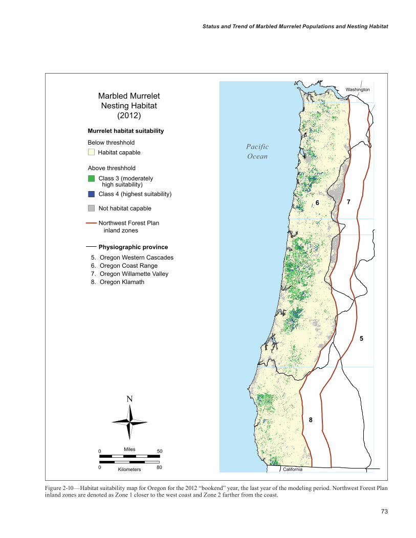
73
Status and Trend of Marbled Murrelet Populations and Nesting Habitat
Washington
7
California
5
8
6
PacificOcean
0 50Miles
0 80Kilometers
Marbled MurreletNesting Habitat
(2012)
Murrelet habitat suitability
Physiographic province
Below threshhold
Above threshhold
Habitat capable
Class 3 (moderately high suitability)Class 4 (highest suitability)
Not habitat capable
Northwest Forest Plan inland zones
Oregon Western CascadesOregon Coast RangeOregon Willamette ValleyOregon Klamath
5.6.7.8.
Figure 2-10—Habitat suitability map for Oregon for the 2012 “bookend” year, the last year of the modeling period. Northwest Forest Plan inland zones are denoted as Zone 1 closer to the west coast and Zone 2 farther from the coast.
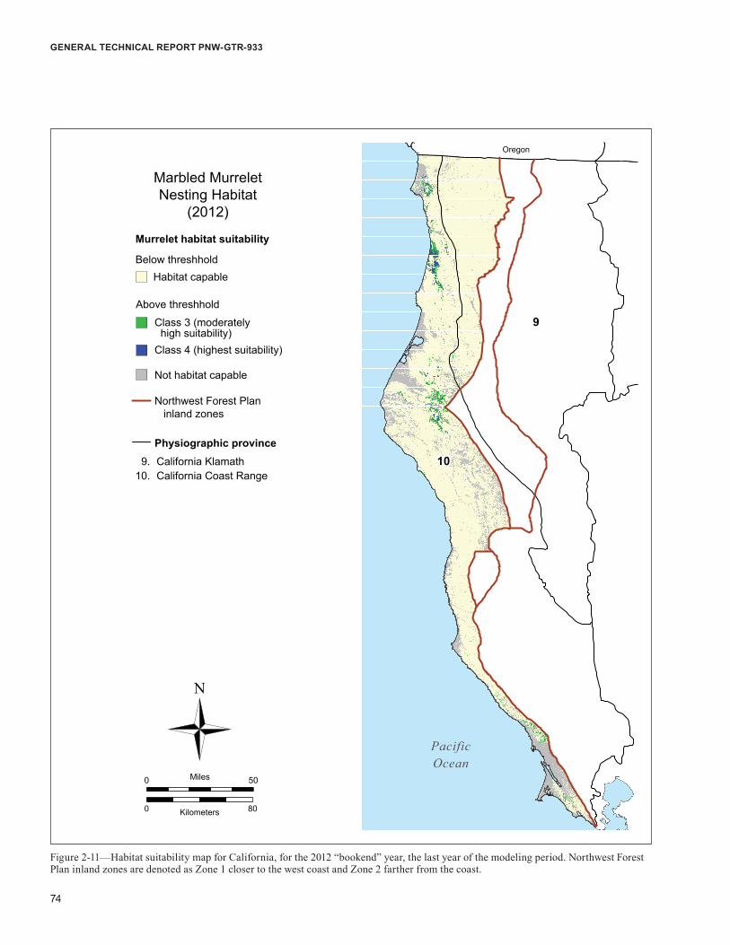
74
GENERAL TECHNICAL REPORT PNW-GTR-933
Oregon
9
10
PacificOcean
0 50Miles
0 80Kilometers
Marbled MurreletNesting Habitat
(2012)
Murrelet habitat suitability
Physiographic province
Below threshhold
Above threshhold
Habitat capable
Class 3 (moderately high suitability)Class 4 (highest suitability)
Not habitat capable
Northwest Forest Plan inland zones
California KlamathCalifornia Coast Range
9.10.
Figure 2-11—Habitat suitability map for California, for the 2012 “bookend” year, the last year of the modeling period. Northwest Forest Plan inland zones are denoted as Zone 1 closer to the west coast and Zone 2 farther from the coast.
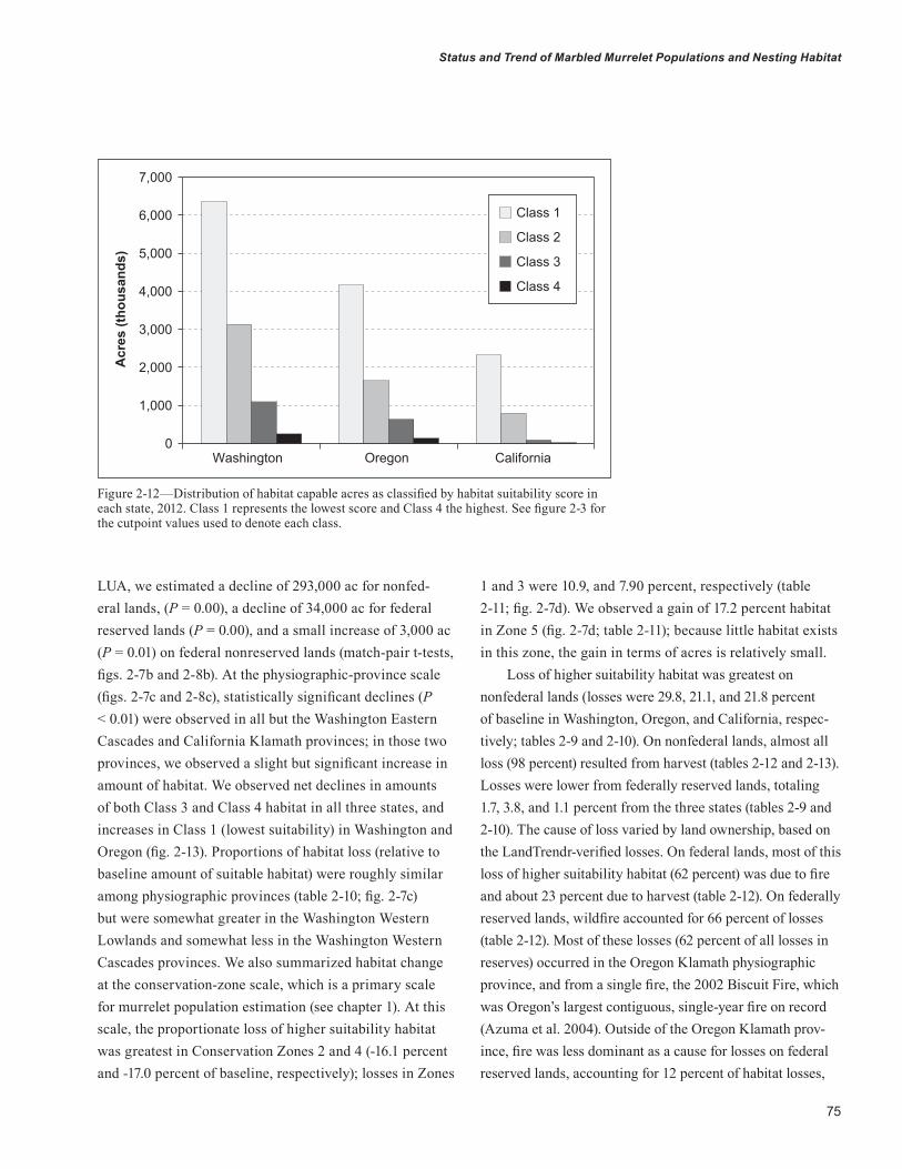
75
Status and Trend of Marbled Murrelet Populations and Nesting Habitat
LUA, we estimated a decline of 293,000 ac for nonfed-eral lands, (P = 0.00), a decline of 34,000 ac for federal reserved lands (P = 0.00), and a small increase of 3,000 ac (P = 0.01) on federal nonreserved lands (match-pair t-tests, figs. 2-7b and 2-8b). At the physiographic-province scale (figs. 2-7c and 2-8c), statistically significant declines (P < 0.01) were observed in all but the Washington Eastern Cascades and California Klamath provinces; in those two provinces, we observed a slight but significant increase in amount of habitat. We observed net declines in amounts of both Class 3 and Class 4 habitat in all three states, and increases in Class 1 (lowest suitability) in Washington and Oregon (fig. 2-13). Proportions of habitat loss (relative to baseline amount of suitable habitat) were roughly similar among physiographic provinces (table 2-10; fig. 2-7c) but were somewhat greater in the Washington Western Lowlands and somewhat less in the Washington Western Cascades provinces. We also summarized habitat change at the conservation-zone scale, which is a primary scale for murrelet population estimation (see chapter 1). At this scale, the proportionate loss of higher suitability habitat was greatest in Conservation Zones 2 and 4 (-16.1 percent and -17.0 percent of baseline, respectively); losses in Zones
1 and 3 were 10.9, and 7.90 percent, respectively (table 2-11; fig. 2-7d). We observed a gain of 17.2 percent habitat in Zone 5 (fig. 2-7d; table 2-11); because little habitat exists in this zone, the gain in terms of acres is relatively small.
Loss of higher suitability habitat was greatest on nonfederal lands (losses were 29.8, 21.1, and 21.8 percent of baseline in Washington, Oregon, and California, respec-tively; tables 2-9 and 2-10). On nonfederal lands, almost all loss (98 percent) resulted from harvest (tables 2-12 and 2-13). Losses were lower from federally reserved lands, totaling 1.7, 3.8, and 1.1 percent from the three states (tables 2-9 and 2-10). The cause of loss varied by land ownership, based on the LandTrendr-verified losses. On federal lands, most of this loss of higher suitability habitat (62 percent) was due to fire and about 23 percent due to harvest (table 2-12). On federally reserved lands, wildfire accounted for 66 percent of losses (table 2-12). Most of these losses (62 percent of all losses in reserves) occurred in the Oregon Klamath physiographic province, and from a single fire, the 2002 Biscuit Fire, which was Oregon’s largest contiguous, single-year fire on record (Azuma et al. 2004). Outside of the Oregon Klamath prov-ince, fire was less dominant as a cause for losses on federal reserved lands, accounting for 12 percent of habitat losses,
0
1,000
2,000
3,000
4,000
5,000
6,000
7,000
Washington Oregon California
Acr
es (t
hous
ands
)
Class 1
Class 2
Class 3
Class 4
Figure 2-12—Distribution of habitat capable acres as classified by habitat suitability score in each state, 2012. Class 1 represents the lowest score and Class 4 the highest. See figure 2-3 for the cutpoint values used to denote each class.

76
GENERAL TECHNICAL REPORT PNW-GTR-933
Washington
Oregon
California
Class 1 Class 2 Class 3 Class 4Habitat suitability class
Class 1 Class 2 Class 3 Class 4Habitat suitability class
Class 1 Class 2 Class 3 Class 4Habitat suitability class
0
500
1,000
1,500
2,000
2,500
3,000
3,500
4,000
4,500
0
500
1,000
1,500
2,000
2,500
3,000
0
1,000
2,000
3,000
4,000
5,000
6,000
7,000
Acr
es (t
hous
ands
)A
cres
(tho
usan
ds)
Acr
es (t
hous
ands
)
19932012
19932012
19932012
A
B
C
Figure 2-13—Acres of habitat within each habitat suitability class at the baseline (1993) and at the end of the modeling period (2012), by state. Higher suitability habitat includes class 3 (moderately high suitability) plus Class 4 (highest suitability). Values are the means from 25 replicated Maxent runs in each state.
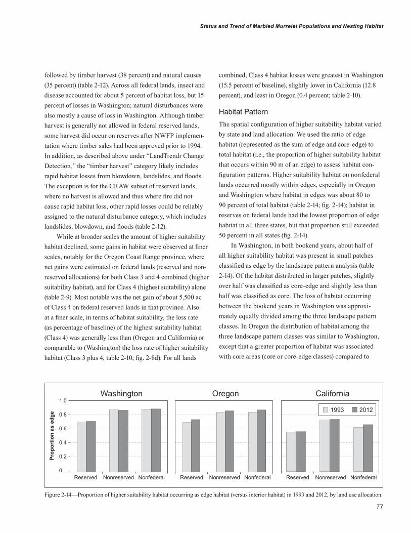
77
Status and Trend of Marbled Murrelet Populations and Nesting Habitat
followed by timber harvest (38 percent) and natural causes (35 percent) (table 2-12). Across all federal lands, insect and disease accounted for about 5 percent of habitat loss, but 15 percent of losses in Washington; natural disturbances were also mostly a cause of loss in Washington. Although timber harvest is generally not allowed in federal reserved lands, some harvest did occur on reserves after NWFP implemen-tation where timber sales had been approved prior to 1994. In addition, as described above under “LandTrendr Change Detection,” the “timber harvest” category likely includes rapid habitat losses from blowdown, landslides, and floods. The exception is for the CRAW subset of reserved lands, where no harvest is allowed and thus where fire did not cause rapid habitat loss, other rapid losses could be reliably assigned to the natural disturbance category, which includes landslides, blowdown, and floods (table 2-12).
While at broader scales the amount of higher suitability habitat declined, some gains in habitat were observed at finer scales, notably for the Oregon Coast Range province, where net gains were estimated on federal lands (reserved and non-reserved allocations) for both Class 3 and 4 combined (higher suitability habitat), and for Class 4 (highest suitability) alone (table 2-9). Most notable was the net gain of about 5,500 ac of Class 4 on federal reserved lands in that province. Also at a finer scale, in terms of habitat suitability, the loss rate (as percentage of baseline) of the highest suitability habitat (Class 4) was generally less than (Oregon and California) or comparable to (Washington) the loss rate of higher suitability habitat (Class 3 plus 4; table 2-10; fig. 2-8d). For all lands
combined, Class 4 habitat losses were greatest in Washington (15.5 percent of baseline), slightly lower in California (12.8 percent), and least in Oregon (0.4 percent; table 2-10).
Habitat PatternThe spatial configuration of higher suitability habitat varied by state and land allocation. We used the ratio of edge habitat (represented as the sum of edge and core-edge) to total habitat (i.e., the proportion of higher suitability habitat that occurs within 90 m of an edge) to assess habitat con-figuration patterns. Higher suitability habitat on nonfederal lands occurred mostly within edges, especially in Oregon and Washington where habitat in edges was about 80 to 90 percent of total habitat (table 2-14; fig. 2-14); habitat in reserves on federal lands had the lowest proportion of edge habitat in all three states, but that proportion still exceeded 50 percent in all states (fig. 2-14).
In Washington, in both bookend years, about half of all higher suitability habitat was present in small patches classified as edge by the landscape pattern analysis (table 2-14). Of the habitat distributed in larger patches, slightly over half was classified as core-edge and slightly less than half was classified as core. The loss of habitat occurring between the bookend years in Washington was approxi-mately equally divided among the three landscape pattern classes. In Oregon the distribution of habitat among the three landscape pattern classes was similar to Washington, except that a greater proportion of habitat was associated with core areas (core or core-edge classes) compared to
0
0.2
0.4
0.6
0.8
1.0
Reserved Nonreserved Nonfederal Reserved Nonreserved Nonfederal
Prop
ortio
n as
edg
e
Washington Oregon California
Reserved Nonreserved Nonfederal
1993 2012
Figure 2-14—Proportion of higher suitability habitat occurring as edge habitat (versus interior habitat) in 1993 and 2012, by land use allocation.

78
GENERAL TECHNICAL REPORT PNW-GTR-933
Tabl
e 2-
9—A
rea
of lo
ss, g
ain,
and
net
cha
nge
in m
arbl
ed m
urre
let h
ighe
r sui
tabi
lity
(Cla
sses
3 p
lus
4) n
estin
g ha
bita
t, an
d ne
t cha
nge
for
the
high
est s
uita
bilit
y (C
lass
4) n
estin
g ha
bita
t, fr
om 1
993
to 2
012,
by
fede
ral l
and
allo
catio
n
Fede
ral n
onre
serv
edFe
dera
l res
erve
dH
ighe
r su
itabi
lity
(Cla
sses
3 +
4)
Cla
ss 4
Hig
her
suita
bilit
y (C
lass
es 3
+ 4
)C
lass
4St
ate
and
prov
ince
Los
ses
Gai
nsN
et c
hang
eN
et c
hang
eL
osse
sG
ains
Net
cha
nge
Net
cha
nge
- - -
- Acr
es -
- - -
Acre
sPe
rcen
tAc
res
Perc
ent
- - -
- Acr
es -
- - -
Acre
sPe
rcen
tAc
res
Perc
ent
Was
hing
ton:
Oly
mpi
c Pe
nins
ula
4,85
75,
812
955
3.4
310
4.31
48,0
3232
,226
-15,
806
-3.0
-1,2
88-1
.00
Wes
tern
Low
land
s1
0-1
-6.2
00
3,65
84,
594
936
7.4
-79
-18.
09W
este
rn C
asca
des
4,93
35,
096
163
0.6
-34
-2.0
344
,071
43,5
96-4
75-0
.2-1
,523
-10.
98Ea
ster
n C
asca
des
739
1,69
395
419
.651
118.
041,
824
2,64
782
36.
9-3
9-2
.73
Was
hing
ton
tota
l10
,530
12,6
012,
071
3.3
327
3.68
97,5
8583
,063
-14,
522
-1.7
-2,9
30-2
.03
Ore
gon:
Coa
st R
ange
8,09
310
,464
2,37
15.
066
210
.40
42,8
8342
,729
-154
0.0
5,53
27.
64W
illam
ette
Val
ley
10
-1-7
.70
00
00
-50.
10
0W
este
rn C
asca
des
00
00
00
43
-1-5
.00
0K
lam
ath
8,72
06,
121
-2,5
99-1
2.0
-273
-11.
8641
,971
22,9
16-1
9,05
5-1
6.3
474
4.07
Ore
gon
tota
l16
,814
16,5
85-2
29-0
.338
94.
4984
,858
65,6
48-1
9,21
0-3
.86,
006
7.15
Cal
iforn
ia:
Coa
st R
ange
222
47-1
75-1
1.1-1
13-2
2.49
1,94
31,
686
-257
-1.0
-125
-1.74
Kla
mat
h70
22-4
8-2
5.1
1-3
1.25
8060
-20
-8.9
00
Cal
iforn
ia to
tal
292
69-2
23-1
2.7
-115
-22.
552,
023
1,746
-277
-1.1
-125
-1.74
Plan
are
a to
tal
27,6
3629
,255
1,61
91.
260
23.
3318
4,46
615
0,45
7-3
4,00
9-2
.52,
952
1.27

79
Status and Trend of Marbled Murrelet Populations and Nesting Habitat
Tabl
e 2-
10—
Are
a of
loss
, gai
n, a
nd n
et c
hang
e in
mar
bled
mur
rele
t hig
her s
uita
bilit
y (C
lass
es 3
plu
s 4)
nes
ting
habi
tat,
and
net c
hang
e fo
r the
hig
hest
sui
tabi
lity
(Cla
ss 4
) nes
ting
habi
tat,
from
199
3 to
201
2, fo
r non
fede
ral a
nd a
ll la
nds
Non
fede
ral
All
land
sH
ighe
r su
itabi
lity
(Cla
sses
3 +
4)
Cla
ss 4
Hig
her
suita
bilit
y (C
lass
es 3
+ 4
)C
lass
4St
ate
and
prov
ince
Los
ses
Gai
nsN
et c
hang
eN
et c
hang
eL
osse
sG
ains
Net
cha
nge
Net
cha
nge
- - -
- Acr
es -
- - -
Acre
sPe
rcen
tAc
res
Perc
ent
- - -
- Acr
es -
- - -
Acre
sPe
rcen
tAc
res
Perc
ent
Was
hing
ton:
Oly
mpi
c Pe
nins
ula
137,
349
50,3
98-8
6,95
1-2
9.1-2
7,187
-27.
3419
0,23
888
,436
-101
,802
-11.
9-2
8,16
5-1
2.0
Wes
tern
Low
land
s13
0,77
848
,785
-81,
993
-32.
0-1
2,35
0-3
8.09
134,
437
53,3
79-8
1,05
8-3
0.1
-12,
429
-37.
8W
este
rn C
asca
des
41,5
4717
,151
-24,
396
-26.
2-3
,782
-36.
3190
,551
65,8
43-2
4,70
8-6
.1-5
,339
-20.
6Ea
ster
n C
asca
des
657
693
362.
74
19.6
13,
220
5,03
31,
813
10.0
161.1
Was
hing
ton
tota
l31
0,33
111
7,02
7-1
93,3
04-2
9.8
-43,
314
-30.
4341
8,44
621
2,69
1-2
05,75
5-1
3.3
-45,
917
-15.
5O
rego
n:C
oast
Ran
ge12
0,23
664
,180
-56,
056
-22.
0-7
,061
-16.
4817
1,21
211
7,37
3-5
3,83
9-7
.8-8
67-0
.7W
illam
ette
Val
ley
165
-11
-66.
20
017
5-1
2-5
7.6
00
Wes
tern
Cas
cade
s2
0-2
-83.
30
06
3-3
-18.
10
0K
lam
ath
12,7
609,
673
-3,0
87-1
1.9
491.
6663
,451
38,71
0-2
4,74
1-1
5.1
250
1.5
Ore
gon
tota
l13
3,01
473
,858
-59,
156
-21.1
-7,0
12-1
5.30
234,
686
156,
091
-78,
595
-9.2
-617
-0.4
Cal
iforn
ia:
Coa
st R
ange
35,8
0112
,503
-23,
298
-22.
3-2
,633
-17.7
237
,966
14,2
36-2
3,73
0-1
8.2
-2,8
71-1
2.7
Kla
mat
h63
182
219
113
.0-1
1-1
6.72
781
904
123
6.6
-12
-17.
5C
alifo
rnia
tota
l36
,432
13,3
25-2
3,10
721
.8-2
,644
-17.7
238
,747
15,14
0-2
3,60
7-1
7.8
-2,8
83-1
2.8
Plan
are
a to
tal
479,7
7720
4,21
0-2
75,5
67-2
6.6
-52,
970
-26.
0869
1,87
938
3,92
2-3
07,9
57-1
2.1
-49,
416
-10.
8
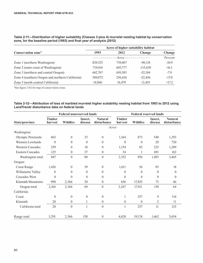
80
GENERAL TECHNICAL REPORT PNW-GTR-933
Table 2-11—Distribution of higher suitability (Classes 3 plus 4) murrelet nesting habitat by conservation zone, for the baseline period (1993) and final year of analysis (2012)
Acres of higher suitability habitatConservation zonea 1993 2012 Change Change
- - - - - - - - - - - - Acres - - - - - - - - - - - - - PercentZone 1 (northern Washington) 829,525 739,407 -90,118 -10.9Zone 2 (outer coast of Washington) 719,414 603,777 -115,638 -16.1Zone 3 (northern and central Oregon) 662,767 610,583 -52,184 -7.9Zone 4 (southern Oregon and northern California) 309,072 256,636 -52,436 -17.0Zone 5 (north-central California) 14,060 16,479 +2,419 +17.2aSee figure 2-02 for map of conservation zones.
Table 2-12—Attribution of loss of marbled murrelet higher suitability nesting habitat from 1993 to 2012 using LandTrendr disturbance data on federal lands
State/province
Federal nonreserved lands Federal reserved landsTimber harvest Wildfire
Insect, disease
Natural disturbance
Timber harvest Wildfire
Insect, disease
Natural disturbance
AcresWashington:
Olympic Peninsula 463 0 33 0 1,164 873 548 1,293Western Lowlands 0 0 0 0 0 0 29 720Western Cascades 259 0 18 0 1,154 82 225 1,289Eastern Cascades 125 0 37 0 34 1 691 163
Washington total 847 0 88 0 2,352 956 1,493 3,465Oregon:
Coast Range 1,426 0 39 0 1,611 56 85 18Willamette Valley 0 0 0 0 0 0 0 0Cascades West 0 0 0 0 0 0 0 0Klamath Mountains 990 2,366 30 0 656 17,855 73 46
Oregon total 2,416 2,366 69 0 2,267 17,911 158 64California:
Coast 8 0 0 0 1 257 9 114Klamath 20 0 1 0 0 0 2 11
California total 28 0 1 0 1 257 11 125
Range total 3,291 2,366 158 0 4,620 19,124 1,662 3,654
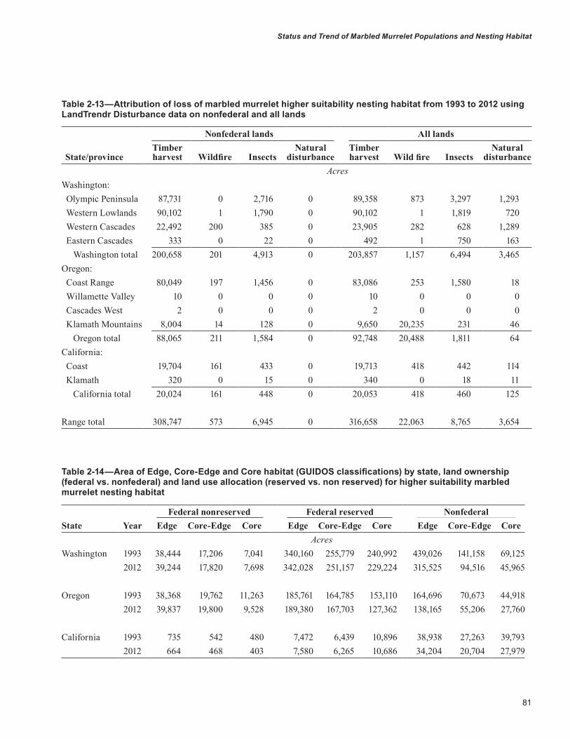
81
Status and Trend of Marbled Murrelet Populations and Nesting Habitat
Table 2-13—Attribution of loss of marbled murrelet higher suitability nesting habitat from 1993 to 2012 using LandTrendr Disturbance data on nonfederal and all lands
State/province
Nonfederal lands All landsTimber harvest Wildfire Insects
Natural disturbance
Timber harvest Wildfire Insects
Natural disturbance
AcresWashington: Olympic Peninsula 87,731 0 2,716 0 89,358 873 3,297 1,293 Western Lowlands 90,102 1 1,790 0 90,102 1 1,819 720 Western Cascades 22,492 200 385 0 23,905 282 628 1,289 Eastern Cascades 333 0 22 0 492 1 750 163 Washington total 200,658 201 4,913 0 203,857 1,157 6,494 3,465Oregon: Coast Range 80,049 197 1,456 0 83,086 253 1,580 18 Willamette Valley 10 0 0 0 10 0 0 0 Cascades West 2 0 0 0 2 0 0 0 Klamath Mountains 8,004 14 128 0 9,650 20,235 231 46 Oregon total 88,065 211 1,584 0 92,748 20,488 1,811 64California: Coast 19,704 161 433 0 19,713 418 442 114 Klamath 320 0 15 0 340 0 18 11 California total 20,024 161 448 0 20,053 418 460 125
Range total 308,747 573 6,945 0 316,658 22,063 8,765 3,654
Table 2-14—Area of Edge, Core-Edge and Core habitat (GUIDOS classifications) by state, land ownership (federal vs. nonfederal) and land use allocation (reserved vs. non reserved) for higher suitability marbled murrelet nesting habitat
State YearFederal nonreserved Federal reserved Nonfederal
Edge Core-Edge Core Edge Core-Edge Core Edge Core-Edge CoreAcres
Washington 1993 38,444 17,206 7,041 340,160 255,779 240,992 439,026 141,158 69,1252012 39,244 17,820 7,698 342,028 251,157 229,224 315,525 94,516 45,965
Oregon 1993 38,368 19,762 11,263 185,761 164,785 153,110 164,696 70,673 44,9182012 39,837 19,800 9,528 189,380 167,703 127,362 138,165 55,206 27,760
California 1993 735 542 480 7,472 6,439 10,896 38,938 27,263 39,7932012 664 468 403 7,580 6,265 10,686 34,204 20,704 27,979
82
GENERAL TECHNICAL REPORT PNW-GTR-933
edge. Habitat losses in Oregon were proportionately greatest from core habitat areas for all land uses, with small gains in the two edge classes on federal lands (table 2-14). In Cali-fornia, the limited amount of nesting habitat was distributed about equally among the three classes, and the loss between bookend years was mainly in core and core-edge habitat, with limited reductions in edge habitat.
Human DisturbanceModeled nesting habitat was strongly correlated with areas of low human footprint. In each of the three states and in both bookend years, over 95 percent of nesting habitat was in five lowest human footprint ranks, more than 80 percent was in three lowest human footprint ranks, and more than 50 percent was in the two lowest human footprint ranks. The most common human footprint rank of nesting habitat in all states was 2 (on a scale of 1 to 10, where 10 is the highest human modification). The mean human footprint rank (table 2-15) within the three landscape pattern classes was approximately equal in Oregon and California in both bookend years; however, in Washington, the human foot-print rank increased somewhat from core habitat to edge (table 2-15). Overall, the mean human footprint rank in all landscape pattern classes was lowest in Washington, highest in California, and intermediate in Oregon.
DiscussionSources of UncertaintyThis work represents a third update of a rangewide map of potential murrelet nesting habitat from consistent baseline vegetation information. We believe the effort has resulted in a more robust understanding of the current amount and distribution of nesting habitat (based on a model using satellite data) compared to the information available at the time of our earlier reports (Raphael et al. 2006, 2011). As in our previous efforts, there are a number of sources of uncertainty that should be recognized.
Vegetation mapping—First, there is uncertainty and error in the underlying GNN vegetation classification. We have previously discussed accuracy assessment information for the vegetation data (see “Methods” above). Error rates in the original vegetation attributes such as tree diameter and canopy cover differed among modeling regions, but on average, the accuracy assessments of the GNN covariates indicated moderate to moderately high accuracy in predicting those attributes, as indicated by correlation coefficients. However, at the scale of GNN modeling region, correlations between GNN predictions and ground-based measurements for pixels, province-scale sometimes fell below 0.5, indicating lower accuracy by the GNN model due to GNN model error in predicting that vegetation attribute within a GNN modeling region. Some of our covariates were derived from combina-tions of GNN covariates (such as PLATFORMS) and we do not have a measure of accuracy of these derived covariates. In general, we can assume that finer scale covariates (such as the count of stems in diameter classes) will be less accu-rate than more broadly defined covariates. Another derived covariate is PCTMATURE_50 and while we have an accuracy assessment for some of the GNN attributes, such as QMDA_DOM and CANCOV, used by GNN to classify pixels as large conifer, we do not know the accuracy of our estimate of the percentage of a 50-ha circle that is classified as large conifer.
Resolution is also a source of uncertainty. In general, finer resolution data, such as the 30-m resolution GNN data, will show more variation and detail than coarser resolution
Table 2-15—Mean human footprint rank (see text) of higher suitability murrelet nesting habitat in edge and core in 1993 and 2012
Habitat patternState Year Core Core-Edge Edge
Washington 1993 2.72 2.85 3.242012 2.63 2.79 3.20
Oregon 1993 3.60 3.63 3.582012 3.64 3.67 3.64
California 1993 3.93 3.88 3.622012 4.02 4.00 3.66
83
Status and Trend of Marbled Murrelet Populations and Nesting Habitat
data. Engler et al. (2004) found that models using higher resolution (finer scale) habitat predictors performed better than models using coarser resolution data (82-ft versus 1,640-ft resolution raster data). The lower model perfor-mances they observed at the 1,640-ft resolution (roughly 62 ac pixel size) were probably caused by a loss of information that is inevitable when aggregating environmental maps. This aggregation may, in some cases, hide important com-binations of habitat predictors that would be expressed with finer resolution data. Our method of computing a 9-pixel average for all covariates helped reduce the effect of errors at the single-pixel scale resulting from imagery noise, while retaining much of the fine-scale richness of the GNN data.
Errors in GNN attribute data also resulted in some model covariate values that did not match the actual vegetation on the ground. For example, we checked GNN attribute data against aerial imagery for murrelet nest and occupied sites used to train the model, and in some cases observed mismatches, where aerial photos showed old forest with large trees, but the GNN attributes for the site indi-cated forest with primarily small trees. This kind of error in the vegetation characteristic data could introduce error into the Maxent models, by training the models on a broader range of ecological conditions at murrelet location sites than actually occurs.
An underlying source of error is noise in the Landsat imagery used by GNN and LandTrendr. Individual Landsat images can have “impulse noise,” which is a general term for single-pixel spots that are not authentic imagery (USGS http://landsat.usgs.gov/science_an_impulsenoise.php). These can results in “salt and pepper” patterns in which individual pixels are misclassified. The LandTrendr procedure of using annual time-series to temporally normalize imagery reduces this error, but does not eliminate it.
Murrelet locations—We recognize three primary sources of uncertainty in our marbled murrelet database. First, for the occupied detection sample we assumed there were no false positives; that is, we assumed murrelets were correctly identified during surveys and that their behavior was correctly observed so that sites with occupied detections were not recorded in
error. Occupied detections were those that were believed to be associated with nesting (Evans Mack et al. 2003), but we cannot know if murrelets were actually nesting at all such detection sites. To the extent that our training sites included occupied sites, which were in fact unsuitable sites, our models could be less accurate by including attribute data from sites that were not actually used by nesting murrelets. Also, our sample of nest sites includes locations where downy young were observed on the ground, or egg fragments were located, and it is possible these signs were not correctly attributed to the actual nest tree or its proximity (especially in the case of egg fragments that could be carried off by predators like ravens). Thus, these sites may have less spatial accuracy than our sample of confirmed nest trees. Third, there is variation in forest attributes among the pixels that we delineated at murrelet locations. Some pixels within areas treated as species sites may not have been the exact locations used by the birds. To the extent that some pixels within 3 x 3-pixel neighborhood that contributed to averaged covariate values for pres-ence locations may have included unsuitable habitat, our description of mean vegetation conditions at the site may have greater variance than a more homogenous site of truly suitable habitat.
Forest changes could have occurred between the year when nesting or occupied behaviors were observed and 1993, the year of the GNN vegetation covariates used in the Maxent models. We reduced this potential source of error by using aerial imagery to confirm the presence of older forest at all training sites in 1993. However, subtler forest changes might have occurred, resulting in a difference between forest conditions at the time murrelets selected a site for nesting and 1993 forest conditions. A related temporal mismatch could occur if marbled murrelet nest selection behavior changed over time. Given the short time period involved in the present analysis, we believe an evolutionary change in nest selection behavior unlikely in a long-lived species. Behavioral changes or forest changes are a consideration for future analysis, particularly in the event of significant changes in forest or environmental attributes associated with climate change.
84
GENERAL TECHNICAL REPORT PNW-GTR-933
The allocation of murrelet location survey effort was not random with respect to the vegetation and physiographic covariates. Murrelet surveys were not conducted according to any planned survey design but, rather, some of the surveys in our database were done in advance of timber sales in forest that was judged likely to be murrelet habitat. As a result, there are likely biases in the distribution of survey effort and hence in the distribution of occupied sites in our dataset (Daw et al. 1998, Edwards et al. 2006, Scott et al. 2002). This could result in a bias that less survey effort was expended in younger forest types with scattered older trees, where the dominant forest is too young to harvest. However, radiotelemetry studies are not subject to this bias and have not found this forest type to be selected often by nesting murrelets (Baker et al. 2006, Manley et al., 2001, Raphael [n.d.], Zharikov et al. 2006). In addition, the standard survey protocol (Evans Mack et al. 2003) recom-mends surveys for any stand where potential nest platforms occur, so surveys do occur in younger stands. The filtering, screening and stratification we conducted on the initial set of occupied sites reduced but did not eliminate the potential for biases in the spatial distribution of training sites within the modeling regions.
Model uncertainty—Projecting model results from one set of environmental data to another set can create uncertainties. We found that the range of values in each of our covariates from the current period fell within the ranges of those covariates in the baseline period, which helps justify our method of projec-tion. However, projecting data in this way assumes that murrelets were selecting habitat conditions in the same way for each time period. If murrelets change habitat preferences in relation to changing environments, then our projections could be inaccurate. We have no evidence that habitat selection has changed.
As noted, our bookend method provides data on both habitat losses and habitat gains. Some of these gains may be due to the different sources of error and uncertainty we have discussed, just as some of the bookend losses may be due to error. Remote sensing approaches have demonstrated their ability to detect both losses and gains in forest cover
(Coops et al. 2010, Hais et al. 2009, Kennedy et al. 2007, Staus et al. 2002), but the ecological characteristics of good murrelet nesting habitat are more complex than simple forest cover. The satellite imagery used to develop GNN covariates, as well as our analytic methods, may be less effective at distinguishing real but gradual increases in hab-itat quality from false gains owing to background random noise, compared to its ability to detect habitat losses fre-quently due to substantial and usually abrupt loss or reduc-tion in forest canopy. For this reason, in a similar analysis for northern spotted owls (Strix occidentalis Caurina) (Davis 2011), the author questioned whether gains identified by bookend models were as reliable as losses of the owl’s complex nesting and roosting habitat, over a short period of analysis. While additional error may occur for projecting a model to a new dataset, versus the error associated with the original model, we used the exact same habitat models and model input sources for both 1993 and 2012, and losses and gains were determined by consistent criteria. However, it is possible that for short analysis periods, there could be more error associated with detecting gains across any suitability threshold value, versus detecting losses across that same threshold, because losses tend to have a stronger signal (greater average loss in suitability) than gains. If this were true, our methods would tend to overestimate gains, and as a consequence underestimate losses when using the “bookend” (net loss) method. We have assumed that model errors are not biased toward losses or gains, but this may be an area for future research. If classification errors occur as a consistent percentage of the pixels in a suitability class, then we might expect a bias toward false gains (more pixels erroneously classified as changing to higher suitability in 2012), versus errors in classifying changes from higher to lower suitability because most (88 percent over the entire NWFP area) of baseline habitat was classified as lower suitability (Class 1 or 2).
Because we performed 25 replicated model runs for each model region, we are able to portray some measure of uncertainty in our prediction of habitat suitability, and in our estimates of habitat change (see figs. 2-7 and 2-8). Doing so represents a major advance in the representation of habitat suitability. The magnitude of variation among
85
Status and Trend of Marbled Murrelet Populations and Nesting Habitat
model runs, represented by the 95-percent confidence interval around estimates, provides a useful way to judge model performance and helps interpret estimates of habitat suitability.
We used presence-only species distribution modeling methods because of the nature of the marbled murrelet nest location data that were available rangewide, notably the lack of adequate and well-distributed samples of absence locations. Given the newness of presence-only methods such as Maxent, caution has been advised in their use (Ahmed et al. 2015, Royle et al. 2012, Yackulic et al. 2013). We exercised caution through the development of our modeling and calibration procedures, during consideration and critical examination of data sources and of modeled relationships between species occurrence and environ-mental covariates, and took steps to minimize potential sampling bias, within the time and resources available for monitoring murrelet nesting habitat. In addition, we have provided information including response curves, model performance metrics, and other information that readers may use to critically evaluate our results.
Notwithstanding these potential errors, our models all had very good (if not excellent) classification skill as measured by the AUC and gain values) and also were well calibrated as evidenced by the P/E (AAF) plots and asso-ciated Spearman test results. The sources of uncertainty we mention should predispose the models to perform worse—not better. Nonetheless, even with the “deck stacked against” good models, good models were generated.
Interpretation of Model OutputWe have presented maps depicting relative suitability of nesting habitat for the murrelet at a resolution of 30 meters. Predicted suitability at a single pixel can be far less reliable than predicted suitability at a larger scale, where small- scale errors are smoothed out by using average suitability over the larger area. Such smoothing can also reduce the accuracy of some single pixels, but predictions at this scale more reliably match the larger scale patterns on the ground. Further, the GNN metadata specifically advises users that the most appropriate use of that data is across landscapes, counties, large watersheds, or ecoregions (areas much larger
than stands or patches). For these reasons, we strongly cau-tion users that estimates of amount of suitable habitat should be based on larger areas, such as for USGS hydrologic units (HUC) (Seaber et al. 1987) of size 6 or larger (that is, HUC codes of 6 or smaller), and not for individual sites or stands. In addition, using our maps to locate specific areas of suitable murrelet habitat on a specific ownership is inappro-priate at any scale, unless combined with ground-truthing or other form of verification.
Comparison With Previous EstimatesResults presented in this report differ from those reported earlier by Raphael et al. (2011). This should be expected, as many aspects of this analysis differ from the earlier work, apart from being based on different bookend years. First, we are now using an updated set of vegetation data (updated GNN models based on a larger sample of vegetation plots) and, for reasons of stronger model predictive accuracy, included correlated covariates in the 20-year models, which was not done previously. Second, for the current analyses, we used the same, and larger set of covariates for each of our three modeling regions, and excluded the Landsat tasseled cap variables (Wetness, Brightness, Greenness) that were included in our previous models. Third, we had a slightly larger set of murrelet locations available with which to train models. Last, we employed different, and we believe superior, criteria for separating habitat suitability Class 1 from Class 2, and Class 3 from Class 4. As a result of these differences, our new baseline estimate of higher suitability habitat over all lands (2.5 million ac) is less than our previous estimate of 3.8 million acres. Also, the current estimate of the highest suitability habitat (Class 4) over all lands (0.46 million ac) is less than our previous estimate of 1.7 million ac (Raphael et al. 2011), but the Class 4 difference was strongly influenced by our change to a new, and biologically based criterion for the division point between Class 3 and Class 4. In summary, the results in this report are the product of updated data, models, and methods and provide, we believe, the best available estimates of the status and trend of marbled murrelet nesting habitat in the NWFP area.

86
GENERAL TECHNICAL REPORT PNW-GTR-933
Implications of ResultsThe NWFP was designed, among its many objectives, to provide habitat conditions that support a viable and well-distributed population of marbled murrelets. The plan is a long-term strategy that is expected to reach its full potential after many decades when previously cutover forest stands within federal reserves mature and begin functioning as suitable habitat. In the short term, the objective is to conserve all remaining habitat, and to that end, the NWFP has conserved to date the large majority (greater than 97 percent) of suitable marbled murrelet nesting habitat that was present on the federal lands NWFP management at the inception of the plan in 1994. Some habitat loss did occur on federal lands, both reserved and nonreserved, during the period of analysis, owing to fire, harvest, and natural disturbances. While some future losses due to wildfire and natural disturbances are likely, harvest losses within federal reserves should drop or cease, with the completion of the “grandfathered” timber sales approved prior NWFP implementation, but harvested after 1993. Over 90 percent of currently higher suitability habitat on federal lands occurs within the various reserve LUAs, but whether this continues is highly dependent on future management and political decisions.
We used a bookend approach to assess gains and losses in higher suitability habitat. We cannot be certain that all gains are real, as some changes may be due to mapping error and other “noise” in the Landsat-based imagery that would cause erroneous estimates. While there is some uncertainty about gains and net change, we believe that a real loss in habitat has occurred from 1993 to 2012. Based on our bookend data, the rate of loss of higher suitability habitat on reserved lands has been about 2.5 percent over the 20-year period (owing mostly to fire, especially in Ore-gon) (table 2-12). However, rate of loss of higher suitability habitat has been about 10 times greater (26.6 percent) on nonfederal lands, owing mostly to timber harvest (table 2-13). Conservation of the threatened murrelet is not possi-ble if such losses continue at this rate into the future.
If the amount of higher suitability habitat for murrelets is to be maintained at its current level, and given that almost half of the higher suitability habitat is on nonfederal lands,
accomplishing this goal will require significant contri-butions from nonfederal lands. Over time, as habitat on federal reserved lands increases in quality, less reliance on nonfederal lands may be warranted. Thus, currently, there are limits on the extent to which the NWFP can protect remaining suitable habitat and prevent its ongoing loss.
We found that the highest suitability habitat (Class 4) comprised a relatively small proportion (about 20 percent) of all higher suitability nesting habitat (Classes 3 plus 4). Class 4 includes areas with suitability scores equaling or exceeding the average condition for the murrelet presence sites used to train our models. To the extent which mur-relets might preferentially nest in this highest suitability habitat, our estimates of the total amount of suitable habitat available to murrelets, as represented by Classes 3 plus 4, may be optimistic.
We estimated a loss of about 34,000 ac of higher suitability habitat (Classes 3 and 4) from federal reserves over the 20 years from 1993 to 2012 (table 2-6). If that rate continued for 50 years (through 2042), the total loss would be about 85,000 ac. There were also over 2 million ac of federally reserved lands in Class 2 condition (i.e., young forest, 37 percent of all habitat-capable reserved lands). Given time, much of this has the potential to develop into more suitable nesting habitat depending on site conditions, presence of older trees, future management and other factors. If 5 percent of the nearly 2 million Class 2 acres developed into higher suitability condition over the next 50 years, that would be more than enough, about 100,000 ac, to balance a loss of 85,000 ac. One must consider, though, that losses of our highest suitability habitat (Class 4) would not be balanced by gains in lower classes of suitability represented by acres that just cross over the habitat suit-ability threshold. In addition, it can take more than 100 years for Class 2 habitat to become Class 3 and more than 200 years to become Class 4. The development of stands with old-growth characteristics necessary for murrelets is expected to take at least 100 to 200 years from the time of regeneration (USFWS 1997). For the many younger stands in the murrelet range that were clear-cut harvested in the past century, the benefits of habitat development are far into the future. However, if management for late-successional
87
Status and Trend of Marbled Murrelet Populations and Nesting Habitat
and old-growth forests continues, projections show substan-tial increases of forest exceeding 150 years in age by 2050 on western federal lands (Mills and Zhou 2003). Shorter term gains in habitat quality may occur as older forest fills in around existing suitable habitat and reduces edge and fragmentation effects in existing habitat, prior to the older forest developing the large limbs, nest platforms, and other characteristics of murrelet nesting habitat.
Over the long run, it is not unreasonable to expect to see some net increase in total amount of higher suitability habitat; however in the short term, conservation of the higher suitability habitat (Classes 3 and 4) is essential. If losses of suitable habitat are reduced, old forest suitable for nesting is allowed to develop, and fragmentation of older forest is reduced throughout the reserved federal lands, then meeting murrelet population objectives will be more certain. Given declining murrelet population trends as well as habitat losses, in many areas, it is uncertain whether their popula-tions will persist to benefit from potential future increases in habitat suitability. This underscores the need to arrest the loss of suitable habitat on all lands, especially on nonfederal lands and in the relatively near term (3 to 5 decades).
AcknowledgmentsThis work would not have been possible without the assis-tance of a large number of people who contributed to the murrelet database and who developed the GNN vegetation datasets. Tom Bloxton helped update some of the murrelet observation databases. Steven Phillips and Ray Davis helped guide us through the use of Maxent software, and Ray provided a sounding board throughout our analyses. Heather Roberts, Matt Gregory, and Janet Ohmann provided GNN data; Warren Cohen, Robert Kennedy, and Zhiqiang Yang provided the LandTrendr data. Murrelet nest locations in Washington were provided by the Washington Depart-ment of Fish and Wildlife (Jane Jenkerson). Nest locations in Oregon were provided by Kim Nelson, the Bureau of Land Management, the U.S. Forest Service Region 6, and the Oregon Department of Forestry. Nest locations in California were provided by Richard Golightly and Stephen Sillett (Humboldt State University), the California Department of Fish and Wildlife (Esther Burkett), the U.S. Fish and Wild-
life Service, the Pacific Lumber Company (David Bigger and Sal Chinnici), and Redwood National and State Parks (Keith Bensen and Amber Transou). We thank Jim Baldwin and Andrew Yost for programming assistance. This paper benefited from comments by Tim Bean, Alan Burger, Ashley Steel, and Andrew Yost. Our work was funded by the USDA Forest Service Pacific Northwest Research Station and Pacific Northwest Region and by the U.S. Fish and Wildlife Service. The findings and conclusions in this article are those of the authors and do not necessarily represent the views of the U.S. Fish and Wildlife Service.
ReferencesAhmed, S.E.; McInerny, G.; O’Hara, K.; Harper, R.;
Salido, L.; Emmott, S.; Joppa, L.N. 2015. Scientists and software—surveying the species distribution modelling community. Diversity and Distributions. 21(3): 258–267.
Alegria, J.L.; Folliard, L.; Lint, J.; Madsen, S.; Webb, L. 2002. Southwest Oregon Inland Survey Assessment for marbled murrelets. Final report submitted to U.S. Fish and Wildlife Service. 39 p.
Azuma, D.L.; Donnegan, J.; Gedney, D. 2004. Southwest Oregon Biscuit Fire. Res. Pap. PNW-RP-560. Portland, OR: U.S. Department of Agriculture, Forest Service, Pacific Northwest Research Station. 32 p.
Baker, L.M.; Peery, M.Z.; Burkett, E.E.; Singer, S.W.; Suddjian, D.L.; Beissinger, S.R. 2006. Nesting habitat characteristics of the marbled murrelet in central California redwood forests. Journal of Wildlife Management. 70: 939–946.
Baldwin, J. 2015. Personal communication. Statistician unit leader, U.S. Department of Agriculture, Forest Service, Pacific Southwest Research Station, 800 Buchanan Street, West Annex Building, Albany, CA 94710.
Baldwin, R.A. 2009. Use of maximum entropy modeling in wildlife research. Entropy. 11: 854–866.
Boyce, M.S.; Vernier, P.R.; Nelson, S.E.; Schmiegelow, F.K.A. 2002. Evaluating resource selection functions. Ecological Modeling. 157: 281–300.

88
GENERAL TECHNICAL REPORT PNW-GTR-933
Burger, A.E. 2002. Conservation assessment of marbled murrelets in British Columbia, a review of the biology, habitat associations and conservation. Technical Report 387. Delta, British Columbia, Canada: Canadian Wildlife Service. 194 p.
Burger, A.E.; Ronconi, R.A.; Silvergieter, M.P.; Conroy, C.; Bahn, V.; Manley, I.A.; Cober, A.; Lank, D.B. 2010. Factors affecting the availability of thick epiphyte mats and other potential nest platforms for marbled murrelets in British Columbia. Canadian Journal of Forest Research. 40(4): 727–746.
Cohen, W.B.; Zhiqiang, Y.; Kennedy, R.E. 2010. Detecting trends in forest disturbance and recovery using yearly Landsat time series: 2. TimeSync tools for calibration and validation. Remote Sensing of Environment. 114: 2911–2924.
Coops, N.C.; Gillanders, S.N.; Wulder, M.A.; Gergel, S.E.; Nelson, T.; Goodwin, N.R. 2010. Assessing changes in forest fragmentation following infestation using time series Landsat imagery. Forest Ecology and Management. 259: 2355–2365.
Davis, R.; Lint, J. 2005. Habitat status and trend. In: Lint, J., tech. coord. Northwest Forest Plan—the first 10 years (1994–2003): status and trends of northern spotted owl populations and habitat. Gen. Tech. Rep. PNW-GTR-648. Portland, OR: U.S. Department of Agriculture, Forest Service, Pacific Northwest Research Station: 21–82. Chapter 3.
Davis, R.J.; Dugger, K.M.; Mohoric, S.; Evers, L.; Aney, W.C. 2011. Northwest Forest Plan—the first 15 years (1994–2008): status and trends of northern spotted owl populations and habitats. Gen. Tech. Rep. PNW-GTR-850. Portland, OR: U.S. Department of Agriculture, Forest Service, Pacific Northwest Research Station. 147 p.
Davis, R.J.; Ohmann, J.L.; Kennedy, R.E.; Cohen, W.B. 2015. Northwest Forest Plan—the first 20 years (1994—2013): status and trends of late-successional and old-growth forests. Gen. Tech. Rep. PNW-GTR-911. Portland, OR: U.S. Department of Agriculture, Forest Service, Pacific Northwest Research Station. 118 p.
Daw, S.K.; DeStefano, S.; Steidl, R.J. 1998. Does survey method bias the description of northern goshawk nest-site structure? Journal of Wildlife Management. 62: 1379–1384.
Edwards, T.C.; Cutler, D.R.; Zimmermann, N.E.; Geiser, L.; Moisen, G.G. 2006. Effects of sample survey design on the accuracy of classification tree models in species distribution models. Ecological Modelling. 199: 132–141.
Elith, J.; Graham, C.H.; Anderson, R.P.; Dudík, M.; Ferrier, S.; Guisan, A.; Hijmans, R.J.; Huettmann, F.; Leathwick, J.R.; Lehmann, A.; Li, J.; Lohmann, L.G.; Loiselle, B.A.; Manion, G.; Moritz, C.; Nakamura, M.; Nakazawa, Y.; Overton, J.M.; Peterson, A.T.; Phillips, S.J.; Richardson, K.S.; Scachetti-Pereira, R.; Schapire, R.E.; Soberón, J.; Williams, S.; Wisz, M.S.; Zimmermann, N.E. 2006. Novel methods improve prediction of species’ distributions from occurrence data. Ecography. 29: 129–151.
Elith, J.; Phillips, S.J.; Hastie, T.; Dudik, M.; Chee, Y.E.; Yates, C.J. 2011. A statistical explanation of MaxEnt for ecologists. Diversity and Distributions 17: 43–57.
Engler, R.; Guisan A.; Rechsteiner, L. 2004. An improved approach for predicting the distribution of rare and endangered species from occurrence and pseudo-absence data. Journal of Applied Ecology. 41: 263–274.
Environmental Research Systems Institute, Inc. [ESRI] c1982–2008. ArcInfo Workstation. Version 9.3. Redlands, CA.
89
Status and Trend of Marbled Murrelet Populations and Nesting Habitat
Environmental Research Systems Institute, Inc. [ESRI] c1999–2009. ArcGIS Desktop 9.3.1. Redlands, CA.
Evans Mack, D.; Ritchie, W.P.; Nelson, S.K.; Kuo-Harrison, E.; Harrison, P.; Hamer, T.E. 2003. Methods for surveying marbled murrelets in forests: a revised protocol for land management and research. Technical Publication Number 2: Pacific Seabird Group. 76 p. http://www.pacificseabirdgroup.org/publications/PSG_TechPub2_MAMU_ISP.pdf. (2 July 2015).
Fielding, A.H.; Bell, J.F. 1997. A review of methods for the assessment of prediction errors in conservation presence/absence models. Environmental Conservation. 24: 38–49.
Forest Ecosystem Management Assessment Team [FEMAT]. 1993. Forest ecosystem management: an ecological, economic, and social assessment. Portland, OR: U.S. Department of Agriculture; U.S. Department of the Interior [and others]. [Irregular pagination].
Franklin, J.F.; Spies, T.A. 1991. Ecological definitions of old-growth Douglas-fir forests. In: Ruggiero, L.F.; Aubry, K.B.; Carey, A.B.; Huff, M., tech. coords. Wildlife and vegetation of unmanaged Douglas-fir forests. Gen. Tech. Rep. PNW-GTR-285. Portland, OR: U.S. Department of Agriculture, Forest Service, Pacific Northwest Research Station: 61–69.
Genuer, R.; Poggi, J-M.; Tuleau-Malot, C. 2010. Variable selection using random forests. Pattern Recognition Letters. 31: 2225–2236.
Gray, A.N. 2003. Monitoring stand structure in mature coastal Douglas-fir forests: effect of plot size. Forest Ecology and Management. 175: 1–16.
Gray, A.N.; Monleon, V.J.; Spies, T.A. 2009. Characteristics of remnant old-growth forests in the northern Coast Range of Oregon and comparison to surrounding landscapes. Gen. Tech. Rep. PNW-GTR-790. Portland, OR: U.S. Department of Agriculture, Forest Service, Pacific Northwest Research Station. 45 p.
Gray, A.N.; Whittier, T.R. 2014. Change in carbon stocks on Pacific Northwest national forests and the role of disturbance, management, and growth. Forest Ecology and Management. 328: 167–178.
Greeley, W.B. 1925. The relation of geography to timber supply. Economic Geography. 1: 1–14.
Guisan, A.; Zimmermann, N.E. 2000. Predictive habitat distribution models in ecology. Ecological Modeling. 135: 147–186.
Hais,M.;Jonášovác,M.;Langhammerd,J.;Kučerac,T. 2009. Comparison of two types of forest disturbance using multitemporal Landsat TM/ETM+ imagery and field vegetation data. Remote Sensing of Environment. 113: 835–845.
Hamer, T.E.; Nelson, S.K. 1995. Characteristics of marbled murrelet nest trees and nesting stands. In: Ralph, C.J.; Hunt, G.L., Jr.; Raphael, M.G.; Piatt, J.F., eds. Ecology and conservation of the marbled murrelet. Gen. Tech. Rep. PSW-GTR-152. Albany, CA: U.S. Department of Agriculture, Forest Service, Pacific Southwest Research Station: 69–82.
Hebert, P.N.; Golightly, R.T. 2008. At-sea distribution and movements of nesting and non-nesting marbled murrelets Brachyramphus marmoratus in northern California. Marine Ornithology. 36: 99–105.
Hemstrom, M.; Spies, T.A.; Palmer, C.J.; Kiester, R.; Teply, J.; McDonald, P.; Warbington, R. 1998. Late-successional and old-growth forest effectiveness monitoring plan for the Northwest Forest Plan. Gen. Tech. Rep. PNW-GTR-438. Portland, OR: U.S. Department of Agriculture, Forest Service, Pacific Northwest Research Station. 37 p.
Henderson, J.A.; Lesher, R.D.; Peter, D.H.; Ringo, C.D. 2011. A landscape model for predicting potential natural vegetation of the Olympic Peninsula USA using boundary equations and newly developed environmental variables. Gen. Tech. Rep. PNW-GTR-841. Portland, OR: U.S. Department of Agriculture, Forest Service, Pacific Northwest Research Station. 35 p.

90
GENERAL TECHNICAL REPORT PNW-GTR-933
Hernandez, P.A.; Graham, C.H.; Master, L.L.; Albert, D.L. 2006. The effect of sample size and species characteristics on performance of different species distribution modeling methods. Ecography. 29: 773–785.
Herold, N.D.; Koeln, G.; Cunnigham, D. 2003. Mapping impervious surfaces and forest canopy using classification and regression tree (CART) analysis. In: Proceedings of the American Society for Photogrammetry and Remote Sensing 2003 annual conference. 7 p. http://nemo.uconn.edu/tools/impervious_surfaces/pdfs/Herold_etal_2003.pdf. (5 January 2011).
Hirzel, A.H.; Hausser, J.; Chessel, D.; Perrin, N. 2002. Ecological-niche factor analysis: How to compute habitat-suitability maps without absence data? Ecology. 83: 2007–2036.
Hirzel, A.H.; Le Lay, G.; Helfer, V.; Randin, C.; Guisan, A. 2006. Evaluating the ability of habitat suitability models to predict species presences. Ecological Modelling. 199: 142–152.
Huff, M.H.; Raphael, M.G.; Miller, S.L.; Nelson, S.K.; Baldwin, J., tech coords. 2006a. Northwest Forest Plan—the first 10 years (1994–2003): status and trends of populations and nesting habitat for the marbled murrelet. Gen. Tech. Rep. PNW-GTR-650. Portland, OR: U.S. Department of Agriculture, Forest Service, Pacific Northwest Research Station. 149 p.
Huff, M.H.; Raphael, M.G.; Miller, S.L.; Nelson, S.K.; Baldwin, J.; Young, R.D.; Brown, M.; Evans-Mack, D. 2006b. Estimating the amount of marbled murrelet nesting habitat on federal lands by using a systematic grid sampling strategy. In: Huff, M.H.; Raphael, M.G.; Miller, S.L.; Nelson, S.K.; Baldwin, J., tech. coords. Northwest Forest Plan—the first 10 years (1994–2003): status and trends of populations and nesting habitat for the marbled murrelet. Gen. Tech. Rep. PNW-GTR-650. Portland, OR: U.S. Department of Agriculture, Forest Service, Pacific Northwest Research Station: 61–95. Chapter 4.
Hunter, J.E.; Schmidt, K.N.; Stauffer, H.B.; Miller, S.L.; Ralph, C.J.; Roberts, L. 1998. Status of the marbled murrelet in the inner north coast ranges of California. Northwestern Naturalist 79: 92–103.
Kennedy, R.E.; Yang, Z.; Cohen, W.B. 2010. Detecting trends in forest disturbance and recovery using yearly Landsat time series: 1. LandTrendr temporal segmentation algorithms. Remote Sensing of Environment. 114: 2897–2910.
Kennedy, R.E.; Yang, Z.; Cohen, W.; Pfaff, E.; Braaten, J.; Nelson, P. 2012. Spatial and temporal patterns of forest disturbance and regrowth within the area of the Northwest Forest Plan. Remote Sensing of Environment. 122: 117–133.
Key, C.H.; Benson, N.C. 2006. Landscape assessment: remote sensing of severity, the normalized burn ratio. In: Lutes, D.C., ed. 2006. FIREMON: Fire effects monitoring and inventory system. Gen. Tech. Rep. RMRS-GTR-164-CD. Fort Collins, CO: U.S. Department of Agriculture, Forest Service, Rocky Mountain Research Station. 1 CD.
Madsen, S.; Evans, D.; Hamer, T.; Henson, P.; Miller, S.; Nelson, S.K.; Roby, D.; Stapanian, M. 1999. Marbled murrelet effectiveness monitoring plan for the Northwest Forest Plan. Gen. Tech. Rep. PNW-GTR-439. Portland, OR: U.S. Department of Agriculture, Forest Service, Pacific Northwest Research Station. 51 p.
Malt, J.; Lank, D. 2007. Temporal dynamics of edge effects on nest predation risk for the marbled murrelet. Biological Conservation. 140(1–2): 160–173.
Manley, I.; Harfenist, A.; Kaiser, G. 2001. Marbled murrelet telemetry study on Queen Charlotte Islands/Haida Gwaii. Unpublished report. On file with: British Columbia Ministry of Environment, Skeena Region, P.O. Box 5000, 3726 Alfred Ave., Smithers, BC V0J2N0.
Manley, I.A.; Nelson, S.K. 1999. Habitat characteristics associated with nest success and predation at marbled murrelet nest trees. Pacific Seabirds. 26: 40.
91
Status and Trend of Marbled Murrelet Populations and Nesting Habitat
Masek, J.G.; Huang, C.Q.; Wolfe, R.; Cohen, W.; Hall, F.; Kutler, J.; Nelson, P. 2008. North American forest disturbance mapped from a decadal Landsat record. Remote Sensing of Environment. 112: 2914–2926.
McComb, W.C.; McGrath, M.T.; Spies, T.A.; Vesely, D. 2002. Models for mapping potential habitat at landscape scales: an example using northern spotted owls. Forest Science. 48: 203–216.
McShane, C.; Hamer, T.; Carter, H.; Swartzman, G.; Friesen, V.; Ainley, D.; Tressler, R.; Nelson, K.; Burger, A.; Spear, L.; Mohagen, T.; Martin, R.; Henkel, L.; Prindle, K.; Strong, S.; Keany, J. 2004. Evaluation report for the 5-year status review of the marbled murrelet in Washington, Oregon, and California. Seattle, WA: EDAW, Inc. http://www.fws.gov/arcata/es/birds/mm/documents/mm5yr_rpt_final_web.pdf. (4 March 2016).
Merow, C.; Silander, J.A. 2014. A comparison of Maxlike and Maxent for modelling species distributions. Methods in Ecology and Evolution. 5: 215–225.
Merow, C.; Smith, J.J.; Silander, J.A. 2013. A practical guide to MaxEnt for modeling species’ distributions: what it does, and why inputs and settings matter. Ecography. 36: 1–12.
Meyer, C.B.; Miller, S.L. 2002. Use of fragmented landscapes by marbled murrelets for nesting in southern Oregon. Conservation Biology 16: 755–766.
Meyer, C.B.; Miller, S.L.; Ralph, C.J. 2002. Multi-scale landscape and seascape patterns associated with marbled murrelet areas on the U.S. west coast. Landscape Ecology 17: 95–115.
Miller, S.L; Ralph, C.J.; Raphael, M.G.; Strong, C.; Thompson, C.W.; Baldwin, J.; Huff, M.H.; Falxa, G.A. 2006. At-sea monitoring of marbled murrelet population status and trend in the Northwest Forest Plan area. In: Huff, M.H.; Raphael, M.G.; Miller, S.L.; Nelson, S.K.; Baldwin, J., tech. coords. Northwest Forest Plan—the first 10 years (1994–2003): status and trends of populations and nesting habitat for the marbled murrelet. Gen. Tech. Rep. PNW-GTR-650. Portland, OR: U.S. Department of Agriculture, Forest Service, Pacific Northwest Research Station: 31–60. Chapter 3.
Miller, S.L.; Raphael, M.G.; Falxa, G.A.; Strong, C.; Baldwin, J.; Bloxton, T.; Galleher, B.M.; Lance, M.; Lynch, D.; Pearson, S.F.; Ralph, C.J.; Young, R.D. 2012. Recent population decline of the marbled murrelet in the Pacific Northwest. Condor. 114: 771–781.
Mills, J.R.; Zhou, X. 2003. Projecting national forest inventories for the 2000 RPA timber assessment. Gen. Tech. Rep. PNW-GTR-568. Portland, OR, U.S. Department of Agriculture, Forest Service, Pacific Northwest Research Station. 58 p.
Moeur, M.; Spies, T.A.; Hemstrom, M.; Alegria, J.; Browning, J.; Cissel, J.; Cohen, W.B.; Demeo, T.E.; Healey, S.; Warbington, R. 2005. Northwest Forest Plan—the first 10 years (1994–2003): status and trend of late-successional and old-growth forest. Gen. Tech. Rep. PNW-GTR-646. Portland, OR: U.S. Department of Agriculture, Forest Service, Pacific Northwest Research Station. 142 p.
Moeur, M.; Ohmann, J.L.; Kennedy, R.E.; Cohen, W.B.; Gregory, M.J.; Yang, Z.; Roberts, H.M.; Spies, T.A.; Fiorella, M. 2011. Northwest Forest Plan—the first 15 years (1994–2008): status and trends of late-successional and old-growth forests. Gen. Tech. Rep. PNW-GTR-853. Portland, OR: U.S. Department of Agriculture, Forest Service, Pacific Northwest Research Station. 48 p.
Morrison, P.H. 1988. Old-growth forests in the Pacific Northwest: a status report. Washington, DC: The Wilderness Society. 46 p.
92
GENERAL TECHNICAL REPORT PNW-GTR-933
Nelson, S.K. 1997. Marbled murrelet (Brachyramphus marmoratus). In: Poole, A.; Gill, F., eds. The birds of North America, No. 276. http://bna.birds.cornell.edu/bna/species/276/articles/introduction. (17 June 2015).
Nelson, S.K. 2015. Unpublished data. On file with: Oregon State University, Department of Fisheries and Wildlife, Oregon Cooperative Fish and Wildlife Research Unit, 104 Nash Hall, Corvallis, OR 97331.
Nelson, S.K.; Huff, M.H.; Miller, S.L.; Raphael, M.G. 2006. Marbled murrelet biology: habitat relations and populations. In: Huff, M.H.; Raphael, M.G.; Miller, S.L.; Nelson, S.K.; Baldwin, J., tech. coords. Northwest Forest Plan—the first 10 years (1994–2003): status and trends of populations and nesting habitat for the marbled murrelet. Gen. Tech. Rep. PNW-GTR-650. Portland, OR: U.S. Department of Agriculture, Forest Service, Pacific Northwest Research Station: 9–30. Chapter 2.
Norheim, R.A. 1996. Is there an answer to mapping old growth? An examination of two projects conducted with remote sensing and GIS. Seattle, WA: University of Washington. 150 p. M.S. thesis.
Norheim, R.A. 1997. Dueling databases: examining the differences between two old growth mapping projects. 13th international symposium on computer-assisted cartography (Auto-Carto 13). http://staff.washington.edu/norheim/oldgrowth/dueling-db.html. (24 June 2015).
Ohmann, J.L.; Gregory, M.J. 2002. Predictive mapping of forest composition and structure with direct gradient analysis and nearest-neighbor imputation in coastal Oregon, U.S.A. Canadian Journal of Forest Research. 32: 725–741.
Ohmann, J.L.; Gregory, M.J.; Roberts, H.M. 2010. GNN “bookend” maps of forest vegetation for NWFP effectiveness monitoring. Unpublished report. On file with: U.S. Department of Agriculture, Forest Service, 1220 SW Third Ave., Portland, OR 97208-3623. 4 p.
Ohmann, J.L.; Gregory, M.J.; Roberts H.M. 2014. Scale considerations for integrating forest inventory plot data and satellite image data for regional forest mapping. Remote Sensing of Environment. 151: 3–15.
Phillips, S.J. [N.d.]. Maxent software for species habitat modeling. http//www.cs.princeton.edu/~schapire/maxent/. (15 January 2016)
Phillips, S.J.; Anderson, R.P.; Schapire, R.E. 2006. Maximum entropy modeling of species geographic distributions. Ecological Modelling. 190: 231–259.
Phillips, S.J.; Dudik, M. 2008. Modeling of species distributions with Maxent: new extensions and a comprehensive evaluation. Ecography. 31: 161–175.
Phillips, S.J.; Elith, J. 2013. On estimating probability of presence from use–availability or presence–background data. Ecology 94: 1409–1419.
PRISM Climate Group. 2012. Northwest Alliance for Computational Science and Engineering. Corvallis, OR: Oregon State University. http://prism.oregonstate.edu. (10 September 2013).
R Core Team. 2013. R: A language and environment for statistical computing. Vienna, Austria: R Foundation for Statistical Computing. http://www.R-project.org/. (19 August 2015).
Ralph, C.J.; Hunt, G.L., Jr.; Raphael, M.G.; Piatt, J.F. 1995. Ecology and conservation of the marbled murrelet in North America: an overview. In: Ralph, C.J.; Hunt, G.L., Jr.; Raphael, M.G.; Piatt, J.F., eds. Ecology and conservation of the marbled murrelet. Gen. Tech. Rep. PSW-GTR-152. Albany, CA: U.S. Department of Agriculture, Forest Service, Pacific Southwest Research Station: 3–22.
Raphael, M.G. [N.d.]. Unpublished data from Breeding Ecology of the marbled murrelet in Washington state study. On file with: U.S. Department of Agriculture, Forest Service, Pacific Northwest Research Station, Forestry Sciences Laboratory, 3625 93rd Ave SW, Olympia, WA 98512.
93
Status and Trend of Marbled Murrelet Populations and Nesting Habitat
Raphael, M.G.; Baldwin, J.; Falxa, G.A.; Huff, M.H.; Lance, M.; Miller, S.L.; Pearson, S.F.; Ralph, C.J.; Strong, C.; Thompson, C. 2007. Regional population monitoring of the marbled murrelet: field and analytical methods. Gen. Tech. Rep. PNW-GTR-716. Portland, OR: U.S. Department of Agriculture, Forest Service, Pacific Northwest Research Station. 70 p.
Raphael, M.G.; Falxa, G.A.; Dugger, K.M.; Galleher, B.M.; Lynch, D.; Miller, S.L.; Nelson, S.K.; Young, R.D. 2011. Northwest Forest Plan—the first 15 years (1994–2008): status and trend of nesting habitat for the marbled murrelet. Gen. Tech. Rep. PNW-GTR-848. Portland, OR: U.S. Department of Agriculture, Forest Service, Pacific Northwest Research Station. 52 p. http://www.fs.fed.us/pnw/pubs/pnw_gtr848.pdf. (2 July 2015).
Raphael, M.G.; Galleher, B.M.; Huff, M.H.; Miller, S.L.; Nelson, S.K.; Young, R.D. 2006. Spatially-explicit estimates of potential nesting habitat for the marbled murrelet. In: Huff, M.H.; Raphael, M.G.; Miller, S.L.; Nelson, S.K.; Baldwin, J., tech. coords. Northwest Forest Plan—the first 10 years (1994–2003): status and trends of populations and nesting habitat for the marbled murrelet. Gen. Tech. Rep. PNW-GTR-650. Portland, OR: U.S. Department of Agriculture, Forest Service, Pacific Northwest Research Station: 97–146. Chapter 5.
Raphael, M.G.; Mack, D.E.; Marzluff, J.M.; Luginbuhl, J.M. 2002. Effects of forest fragmentation on populations of the marbled murrelet. Studies in Avian Biology. 25: 222–236.
Raphael, M.G.; Young, J.A.; Galleher, B.M. 1995. A landscape-level analysis of marbled murrelet habitat in western Washington. In: Ralph, C.J.; Hunt, G.L., Jr.; Raphael, M.G.; Piatt, J., tech. coords. Ecology and conservation of the marbled murrelet. Gen. Tech. Rep., PSW-GTR-152. Albany, CA: U.S. Department of Agriculture, Forest Service, Pacific Southwest Research Station: 177–198.
Royle, J.A.; Richard B. Chandler, R.B.; Yackulic, C.; Nichols, J.D. 2012. Likelihood analysis of species occurrence probability from presence-only data for modelling species distributions. Methods in Ecology and Evolution. 3: 545–554.
Sawyer, J.O.; Sillett, S.C.; Libby, W.J.; Dawson, T.E.; Popenoe, J.H.; Largent, D.L.; Van Pelt, R.; Veirs, S.D., Jr.; Noss, R.F.; Thornburgh, D.A.; Del Tredici, P. 2000. Redwood trees, communities and ecosystems: a closer look. In: Noss, R.F., ed. The redwood forest: history, ecology, and conservation of the coast redwoods. Washington DC: Island Press: 81–118.
Scott,J.M.;Heglund,P.J.;Morrison,M.L.;Haufler,J.B.; Raphael, M.G.; Wall, W.A.; Samson, F.B., eds. 2002. Predicting species occurrences: issues of accuracy and scale. Washington, DC: Island Press. 840 p.
Seaber, P.R.; Kapinos, F.P.; Knapp, G.L. 1987. Hydrologic unit maps. Water-Supply Paper 2294. Reston, VA: U.S. Department of the Interior, Geological Survey. 63 p. http://water.usgs.gov/GIS/huc.html. (24 June 2015)
Spies, T.A.; Franklin, J.F. 1988. Old growth and forest dynamics in the Douglas-fir region of western Oregon and Washington. Natural Areas Journal. 8: 190–201.
Spies, T.A.; Johnson, K.N.; Burnett, K.M.; Ohmann, J.L.; McComb, B.C.; Reeves, G.H.; Bettinger, P.; Kline, J.D.; Garber-Yonts, B. 2007. Cumulative ecological and socioeconomic effects of forest policies in coastal Oregon. Ecological Applications. 17: 5–17.
Staus, N.L.; Strittholt, J.R.; DellaSala, D.A.; Robinson, R. 2002. Rate and pattern of forest disturbance in the Klamath-Siskiyou ecoregion, USA between 1972 and 1992. Landscape Ecology. 17: 455–470.
Thomas, J.W.; Franklin, J.F.; Gordon, J.; Johnson, K.N. 2006. The Northwest Forest Plan: origins, components, implementation experience, and suggestions for change. Conservation Biology. 20: 277–287.
94
GENERAL TECHNICAL REPORT PNW-GTR-933
U.S. Department of Agriculture, Forest Service [USDA FS]. 2008. Forest health protection aerial survey data. http:// www.fs.fed.us/r6/nr/fid/as/index.shtml. (4 January 2011).
U.S. Department of Agriculture, Forest Service; U.S. Department of the Interior, Bureau of Land Management [USDA and USDI]. 1994a. Final supplemental environmental impact statement on management of habitat for late-successional and old-growth forest related species within the range of the northern spotted owl (Northwest Forest Plan). Portland, OR. 2 vol.
U.S. Department of Agriculture, Forest Service; U.S. Department of the Interior, Bureau of Land Management [USDA and USDI]. 1994b. Record of decision for amendments to Forest Service and Bureau of Land Management planning documents within the range of the northern spotted owl. [Place of publication unknown]. 74 p. [plus attachment A: standards and guidelines].
U.S. Department of the Interior, Fish and Wildlife Service [USFWS]. 1997. Recovery plan for the threatened marbled murrelet (Brachyramphus marmoratus) in Washington, Oregon, and California. Portland, OR. 203 p.
Van Wagtendonk, J.W.; Root, R.R.; Key, C.H. 2004. Comparison of AVIRIS and Landsat ETM+ detection capabilities for burn severity. Remote Sensing of Environment. 92: 397–408.
Vogelmann, J.E.; Howard, S.M.; Yang, L.; Larson, C.R.; Wylie, B.K.; Van Driel, J.N. 2001. Completion of the 1990’s national land cover dataset for the conterminous United States. Photogrammetric Engineering and Remote Sensing. 67: 650–662.
Vogt, P. 2013. GUIDOS: tools for the assessment of pattern, connectivity, and fragmentation. Vienna, Austria: EGU General Assembly 2013: 13526.
Yackulic, C.B.; Chandler, R.; Zipkin, E.F.; Royle A.J; Nichols, J.D.; Campbell Grant, E.H.; Vera, S. 2013. Presence-only modelling using MAXENT: when can we trust the inferences? Methods in Ecology and Evolution. 4: 236–243.
Zharikov, Y.; Lank, D.B.; Huettmann, F.; Bradley, R.W.; Parker, N.; Yen, P.P.-W.; Mcfarlane-Tranquilla, L.A.; Cooke, F. 2006. Habitat selection and breeding success in a forest-nesting alcid, the marbled murrelet, in two landscapes with different degrees of forest fragmentation. Landscape Ecology. 21: 107–120.

95
Status and Trend of Marbled Murrelet Populations and Nesting Habitat
Chapter 3: Factors Influencing Status and Trend of Marbled Murrelet Populations: An Integrated PerspectiveMartin G. Raphael,1 Andrew J. Shirk,2 Gary A. Falxa,3 Deanna Lynch,4 S. Kim Nelson,5 Scott F. Pearson,6 Craig Strong,7 and Richard D. Young8
SummaryThe Northwest Forest Plan (NWFP) was implemented, in part, to provide habitat conditions that would contribute to the conservation and recovery of threatened species including the marbled murrelet (Brachyramphus marmoratus). Effective-ness monitoring of marbled murrelet populations and nesting habitat helps inform land managers whether this objective is being met. The murrelet depends upon the marine environ-ment to meet its foraging and roosting requirements and upon terrestrial forest to meet its nesting requirements. To assess the relative contributions of terrestrial and marine factors on murrelet population abundance and distribution, we synthe-sized data on the status and trend of murrelet populations, status and trend of inland nesting habitat, and status and trend of marine factors. Specifically, we initially examined the spatial and temporal correlations of marine and terrestrial factors with the spatial distribution and trend of murrelets. We then used a boosted regression tree analysis to investigate the contributions of a suite of marine and terrestrial factors to at-sea murrelet abundance. In both analyses, we found that numbers of murrelets are strongly correlated with amounts and pattern (large contiguous patches) of suitable nesting
habitat, and population trend is most strongly correlated with trend in nesting habitat, although marine factors may also contribute to this trend. Model results suggest that conservation of suitable nesting habitat is key to murrelet conservation. Conservation of habitat within reserves, as well as management actions that are designed to minimize loss of suitable habitat or improve quality of nesting habitat, will likely contribute to murrelet conservation and recovery.
IntroductionThe primary objective of the Marbled Murrelet Effec-tiveness Monitoring Program is to assess the degree to which land management under the NWFP is contributing to the NWFP goal of stabilizing and increasing murrelet populations by maintaining and increasing murrelet nesting habitat in the NWFP area (Madsen et al. 1999). This objective and goal were motivated by the original charter for the Forest Ecosystem Management Assessment Team (FEMAT) report that called for development of long-term management alternatives that would provide “maintenance and/or restoration of habitat conditions for…the marbled murrelet that will provide for viability” (FEMAT 1993:iv). The murrelet nests on forested lands but feeds, roosts, and spends the majority of its time in the marine environment. Forest managers can directly influence only the bird’s nesting habitat quantity and quality; the management of marine habitat, while important to murrelet conservation, is under the purview of management and regulatory bodies outside of the NWFP. Because the NWFP is a land-based forest ecosystem management program, the ultimate goal of the murrelet effectiveness monitoring program is to relate population trends to the amount and distribution of nesting habitat (Madsen et al. 1999). A long-term objective of the monitoring program is to “[e]xamine predictive relationships between marbled murrelets and nesting habitat conditions in the NWFP area so that trends in nesting habitat might eventually suffice as a surrogate for trends in murrelet populations” (Madsen et al. 1999).
1 Research wildlife biologist, U.S. Department of Agriculture, Forest Service, Pacific Northwest Research Station, 3625 93rd Ave. SW, Olympia WA 98512. 2 Ecologist, Climate Impacts Group, College of the Environment, University of Washington, Box 355674, Seattle, WA 98195. 3 Fish and wildlife biologist, U.S. Fish and Wildlife Service, Arcata Fish and Wildlife Office, 1655 Heindon Rd., Arcata, CA 95521. 4 Fish and wildlife biologist, U.S. Fish and Wildlife Service, Wash-ington Fish and Wildlife Office, Branch of Listing, 510 Desmond Dr., Suite 102, Lacey, WA 98503. 5 Research wildlife biologist, Oregon Cooperative Fish and Wildlife Research Unit, Oregon State University, Department of Fisheries and Wildlife, 104 Nash Hall, Corvallis, OR 97331. 6 Senior scientist, Wildlife Science Division, Washington Depart-ment of Fish and Wildlife, 1111 Washington St. SE, 5th Floor, Olympia, WA 98501. 7 Consultant researcher, Crescent Coastal Research, 7700 Bailey Road, Crescent City, CA 95531. 8 Geospatial information system analyst, U.S. Fish and Wildlife Service, Pacific Regional Office, Ecological Services, 911 NE 11th Avenue, Portland, OR 97232.

96
GENERAL TECHNICAL REPORT PNW-GTR-933
This chapter reports on initial steps toward the long-term objective of relating nesting habitat conditions to the distribution and trend of marbled murrelet populations at sea. It builds on the findings of the at-sea population monitoring (chapter 1) and of inland nesting habitat (chapter 2). Because of the potential for both marine and terrestrial influences on murrelet populations, we explored the relative contributions of both marine (foraging and survival) and terrestrial (nesting and fecundity) factors on murrelet abundance and distribution. This research is intended to help managers assess whether current management of nesting habitat on federal lands within the NWFP area is sufficient or needs to be modified, or if agencies also need to influence management of nonfederal lands and marine factors to stabilize and increase murrelet populations. This chapter provides a brief synthesis of the results of these initial steps plus the results of the population and habitat monitoring chapters in this report, as well as a discussion of management implications of those results.
MethodsUnivariate CorrelationsTo address the influences of marine and terrestrial factors on murrelet status and trend, we first examined potential associations between the distribution of murrelets at-sea and individual factors describing the adjacent marine and terrestrial environments during the nesting season (May to September). We did this by examining simple correlations between individual marine and terrestrial factors and murrelet populations in space and time. Our intent here was to conduct some data explorations to see if there might be relationships. For this exploratory work, we summarized estimates of higher suitability nesting habitat for 2012 obtained from the work reported in chapter 2. We also cal-culated the fragmentation of that nesting habitat by using the patch cohesion metric in Fragstats (McGarigal et al. 2012).
We hoped to assess the influence of the marbled mur-relet’s primary prey, forage fish, on murrelet populations. However, we found only one forage-fish dataset that occurs in our area of interest (Emmett 2014). To our knowledge, there are no other forage fish datasets available for the five conservation zones in the NWFP area (Conservation Zones
1 through 5 as defined by the marbled murrelet recovery plan [USFWS 1997]). For analysis of trends in the broader study area, we examined a set of readily available physical and biological ocean factors that have been used in similar multivariate analyses in other studies (e.g., Ainley and Hyrenbach 2010) that we felt might serve as proxies for murrelet prey. Sea surface temperature and chlorophyll con-centration are factors that affect marine productivity. Cooler waters are enriched with nutrients compared with warmer waters; chlorophyll A concentration is related to primary productivity. Our assumption is that cooler waters with enriched chlorophyll A should support higher prey biomass than warmer waters or waters with lower chlorophyll A. We obtained data from a season corresponding with murrelet breeding activity, and also from the previous winter, think-ing that there could be time lags between those factors and their ultimate influence on space use by murrelets.
We then summarized these data at several spatial lev-els: state (Washington, Oregon, California); Conservation Zones 1 through 5; and stratum (conservation zones broken down by coastal areas as described in Raphael et al. 2007, n = 9, fig. 3-1). The analyses reported here used two strata in each conservation zone except for Zone 1 (Strait of Juan de Fuca, San Juan Islands, and Puget Sound). We treated Conservation Zone 1 as a single stratum, rather than using the three strata used in population sampling (fig. 3-1). We did this because the complex geography of coastal waters and potential nesting habitat in Conservation Zone 1 allows birds from multiple at-sea strata to access nesting habitat throughout the zone. By comparison, in all other zones, the geography was that of a roughly linear band of coastal waters matched with a roughly linear band of potential nest-ing habitat inland. To assess the correlation between amount of nesting habitat with sampling strata and adjacent mur-relet population size, we first adjusted for stratum area by regressing amount of habitat and number of birds with total land area of each stratum. We then saved the residuals from these regressions and computed the correlation between residual murrelet abundance and residual habitat area.
In examining trends over time, we were able to obtain data on abundance of forage fish from two transects used to sample forage fish abundance (R. Emmett, 2014.), each in
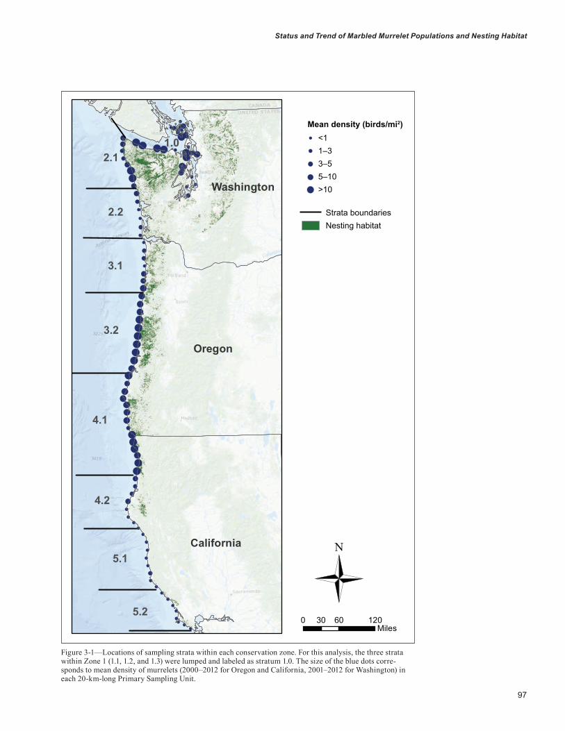
97
Status and Trend of Marbled Murrelet Populations and Nesting Habitat
1.02.1
2.2
3.1
4.1
4.2
5.1
5.2
3.2Oregon
California
Washington
0 60 12030Miles
Mean density (birds/mi2)<11–33–55–10>10
Strata boundariesNesting habitat
Figure 3-1—Locations of sampling strata within each conservation zone. For this analysis, the three strata within Zone 1 (1.1, 1.2, and 1.3) were lumped and labeled as stratum 1.0. The size of the blue dots corre-sponds to mean density of murrelets (2000–2012 for Oregon and California, 2001–2012 for Washington) in each 20-km-long Primary Sampling Unit.

98
GENERAL TECHNICAL REPORT PNW-GTR-933
proximity to two of our murrelet sampling strata; one near the southern part of Conservation Zone 2, and one near the northern end of Conservation Zone 3 (fig. 3-1). We com-pared annual estimates of murrelet abundance in each of these two strata to annual estimates of fish abundance over the available years 2003 to 2011.
Before doing correlations, we examined each factor for spatial and temporal autocorrelations. We found weak evidence of both spatial and temporal autocorrelation for some factors in at least one geographic area; therefore, p-values are not strictly interpretable. For that reason, we do not report p-values and describe the correlation coef-ficients as indicators of possible trends or indications of potential relationships.
Multivariate Model We then developed a quantitative, multivariate model with a goal to assess concurrently the relative strength of marine and terrestrial factors in predicting the spatial and temporal abundance of marbled murrelets. To better under-stand the combined influences of marine and terrestrial factors on marbled murrelet distribution and population trends at sea, we constructed a set of multivariate models that simultaneously account for each marine and terrestrial factor as well as their interactions in space and time. For this analysis, we used boosted regression tree (BRT) models, generally following methods detailed in Raphael et al. (2015) but with three changes. First, the analysis scale was expanded from 5-km nearshore segments to a sample unit comprising an entire primary sampling unit (PSU). Each PSU consisted of an approximately 20-km long coastal segment with both nearshore and offshore sampling areas (chapter 1 describes the sampling design). In Raphael et al. (2015), the analysis was performed at the scale of 5-km nearshore segments because those authors were interested in fine-scale habitat associations and identification of “hotspots” of murrelet abundance along the coast. This current analysis more closely matches the design of population sampling reported in chapter 1. Second, the analysis was extended to include data through 2012. Third, the environmental attribute for “distance to shore” was dropped because it is not relevant when the full
PSU is used as the sample unit (environmental attributes are shown in table 3-1). The sample size in this analysis totaled 1,099 PSU-year combinations; numbers of PSUs varied from 81 to 94 in any particular year depending on which PSUs were sampled each year.
We calculated all covariates annually from 2000–2012 for each PSU, except for Zones 1 and 2, where we used 2001–2012 because population data was not available for 2000. Covariates varied spatially (by PSU), temporally (by year), or both spatially and temporally (table 3-1). Covariates were also associated with either marine foraging habitat suitability or terrestrial nesting habitat suitability (table 3-1). While the habitat status and trend analysis (chapter 2) focused on habitat conditions for two “bookend” years (1993 and 2012), as described below we estimated the amount of suitable nesting habitat in each of the years from 2000 (or 2001) to 2012.
The first two marine covariates in table 3-1 were based on proximity to terrestrial features that may influence observed at-sea abundance of murrelets, presumably due to effects on foraging conditions. These included the distance (in kilometers) from the PSU center to the nearest major river (defined by a flow > 166 ft3/sec [4.7 m3/sec] based on USGS Enhanced River Reach Data 2.0 from 2003), and the predominant shoreline type. Shorelines were classified based on the Environmental Sensitivity Index (ESI) classi-fication system (NOAA 2002), which categorizes shorelines into 21 major classes. We simplified these into 11 classes and then calculated the majority shoreline type within each PSU boundary. This calculation resulted in eight types represented in our study area (table 3-2).
The next set of marine covariates in table 3-1 was based on oceanographic conditions that may influence prey availability (primarily forage fish) and therefore murrelet abundance at sea. Because foraging conditions within each PSU are likely to be influenced by marine conditions at broader scales, we calculated the remaining marine covari-ates that vary spatially based on the mean or sum (depend-ing on the covariate) of values within a 10-km moving window. We then extracted the mean values of the moving window result within each PSU (i.e., the mean of all moving window centers that fell within the PSU).
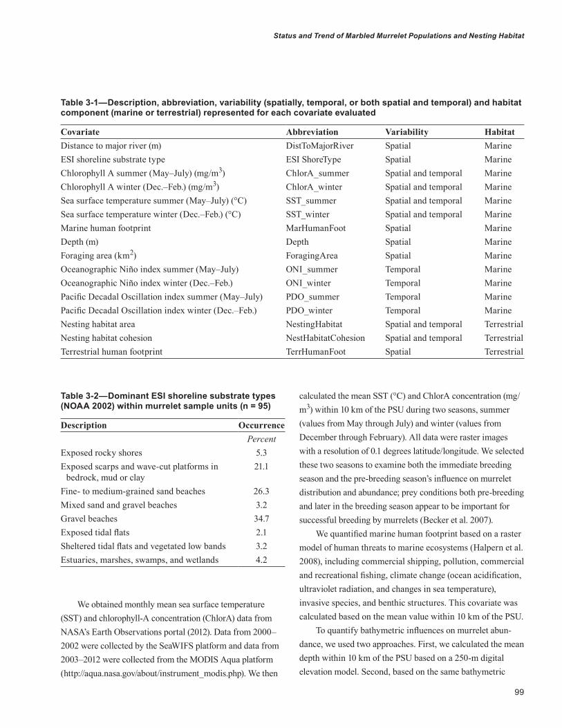
99
Status and Trend of Marbled Murrelet Populations and Nesting Habitat
We obtained monthly mean sea surface temperature (SST) and chlorophyll-A concentration (ChlorA) data from NASA’s Earth Observations portal (2012). Data from 2000–2002 were collected by the SeaWIFS platform and data from 2003–2012 were collected from the MODIS Aqua platform (http://aqua.nasa.gov/about/instrument_modis.php). We then
calculated the mean SST (°C) and ChlorA concentration (mg/m3) within 10 km of the PSU during two seasons, summer (values from May through July) and winter (values from December through February). All data were raster images with a resolution of 0.1 degrees latitude/longitude. We selected these two seasons to examine both the immediate breeding season and the pre-breeding season’s influence on murrelet distribution and abundance; prey conditions both pre-breeding and later in the breeding season appear to be important for successful breeding by murrelets (Becker et al. 2007).
We quantified marine human footprint based on a raster model of human threats to marine ecosystems (Halpern et al. 2008), including commercial shipping, pollution, commercial and recreational fishing, climate change (ocean acidification, ultraviolet radiation, and changes in sea temperature), invasive species, and benthic structures. This covariate was calculated based on the mean value within 10 km of the PSU.
To quantify bathymetric influences on murrelet abun-dance, we used two approaches. First, we calculated the mean depth within 10 km of the PSU based on a 250-m digital elevation model. Second, based on the same bathymetric
Table 3-1—Description, abbreviation, variability (spatially, temporal, or both spatial and temporal) and habitat component (marine or terrestrial) represented for each covariate evaluated
Covariate Abbreviation Variability HabitatDistance to major river (m) DistToMajorRiver Spatial MarineESI shoreline substrate type ESI ShoreType Spatial MarineChlorophyll A summer (May–July) (mg/m3) ChlorA_summer Spatial and temporal MarineChlorophyll A winter (Dec.–Feb.) (mg/m3) ChlorA_winter Spatial and temporal MarineSea surface temperature summer (May–July) (°C) SST_summer Spatial and temporal MarineSea surface temperature winter (Dec.–Feb.) (°C) SST_winter Spatial and temporal MarineMarine human footprint MarHumanFoot Spatial MarineDepth (m) Depth Spatial MarineForaging area (km2) ForagingArea Spatial MarineOceanographic Niño index summer (May–July) ONI_summer Temporal MarineOceanographic Niño index winter (Dec.–Feb.) ONI_winter Temporal MarinePacific Decadal Oscillation index summer (May–July) PDO_summer Temporal MarinePacific Decadal Oscillation index winter (Dec.–Feb.) PDO_winter Temporal MarineNesting habitat area NestingHabitat Spatial and temporal TerrestrialNesting habitat cohesion NestHabitatCohesion Spatial and temporal TerrestrialTerrestrial human footprint TerrHumanFoot Spatial Terrestrial
Table 3-2—Dominant ESI shoreline substrate types (NOAA 2002) within murrelet sample units (n = 95)
Description OccurrencePercent
Exposed rocky shores 5.3Exposed scarps and wave-cut platforms in
bedrock, mud or clay21.1
Fine- to medium-grained sand beaches 26.3Mixed sand and gravel beaches 3.2Gravel beaches 34.7Exposed tidal flats 2.1Sheltered tidal flats and vegetated low bands 3.2Estuaries, marshes, swamps, and wetlands 4.2
100
GENERAL TECHNICAL REPORT PNW-GTR-933
data, we summed the area (km2) of depths suitable for foraging within 10 km of the PSU, hereafter referred to as “foraging area.” Suitable foraging depths were based on a threshold (<25 m deep, except for the San Juan Islands and northern Puget Sound, for which the threshold was <40 m); the thresholds were based on natural breaks observed in the plots of murrelet abundance versus depth.
The last four marine covariates were indices of broader Pacific Ocean conditions, including the Pacific Decadal Oscillation (PDO) (Mantua et al. 1997) and the El Niño Southern Oscillation (ENSO) (Trenberth 1997). The PDO index (JISAO 2012) is based on variation in North Pacific SST from 1900 to the present. The Oceanic Niño Index (ONI), a measure of the state of the ENSO, is based on variation in equatorial Pacific SST (NOAA 2012b). Both indices are calculated on a monthly basis, which we then averaged for two seasons, summer (values from May through July, representing conditions during the central murrelet nesting season) and winter (values from December through February, representing the period preceding nesting).
To quantify the terrestrial habitat influences on at-sea marbled murrelet abundance, we calculated three covariates that quantified the amount and fragmentation of nesting habitat as well as degradation by human modifica-tion. Because murrelets can commute up to at least 80 km from foraging to nesting sites (Hébert and Golightly 2008; Nelson 1997; Raphael and Bloxton, unpublished data) we calculated each of these terrestrial covariates within an 80-km moving window. We then calculated the mean of the moving window result within each PSU (i.e., all moving window centers that fell within the PSU bound-ary). Although our main study area did not extend north of Washington state, in some areas of Washington the 80-km window included terrestrial habitat in British Columbia, Canada. We quantified terrestrial nesting habitat based on a marbled murrelet nesting habitat spatial model produced for the U.S. portion of our study area (chapter 2). This model classified nesting habitat into four classes where Classes 1 and 2 were lower suitability and Classes 3 and 4 were higher suitability. For our analysis, we converted the suitability map into a binary model and defined the
combination of Classes 3 and 4 as higher suitability nesting habitat. For British Columbia terrestrial areas, we defined nesting habitat based on areas designated by the Ministry of Forests, Lands, and Natural Resource Oper-ations as Old Growth Management areas (FLNRO 2012). Temporal variation in higher suitability nesting habitat was represented by modeling habitat changes between 2000 and 2012. We did this by overlaying annual locations of forest disturbance (e.g., timber harvest, fire, windthrow) obtained from the LandTrendR files as described in chapter 2. At each year, we then reclassified any habitat within the disturbed area for that year from higher to lower suitabil-ity. We also calculated the fragmentation of nesting habitat using the patch cohesion metric in Fragstats (McGarigal et al. 2012) within an 80-km radius moving window. Finally, we calculated the mean terrestrial human footprint within an 80-km moving window based on a model of anthropogenic landscape modifications (including human habitation), roads, railroads, irrigation canals, power lines, linear feature densities, agricultural land, campgrounds, highway rest stops, landfills, oil and gas development, and human-induced fires (Leu et al. 2008).
We used boosted regression trees with a Poisson loss function to explore the relationship between murrelet at-sea abundance and our suite of marine and terrestrial covari-ates. Boosted regression tree (BRT) is a machine-learning approach combining regression trees with a boosting pro-cedure that adds new trees to the model fit to the residuals of the prior trees (Elith et al. 2008). The BRT prediction is optimized based on two main parameters, the learning rate and tree complexity. The learning rate, also called shrink-age rate, determines the contribution of each new tree added to the model, while tree complexity determines the number of nodes per tree. Following recommendations of Elith et al. (2008), we used a learning rate of 0.01 and a tree complexity of 5 throughout our analysis. The optimal number of trees was selected based on training the model to one half of the data and then assessing the fit of the model to the remaining half. When new trees began to reduce the fit of the model to the test data, no new trees were added. Final model parame-ters were derived from an ensemble of all trees weighted by the learning rate.

101
Status and Trend of Marbled Murrelet Populations and Nesting Habitat
Because our sample units were contiguous 20-km segments of coastal waters, they might exhibit spatial autocorrelation; spatial autocorrelation occurs when the covariate values of two sample units are related to their distance apart. To account for spatial autocorrelation in the BRT model residuals, we calculated a residual autocovariate term (RAC), as in Crase et al. (2012), by plotting the residuals from the BRT model to raster grid cells representing each survey segment, calculating the mean residual within a 25-km moving window, and then extracting the moving window result for each PSU grid cell. We then refit the BRT model as before but including the RAC term.
We assessed variable importance based on the number of times a variable was used for splitting weighted by the squared loss of deviance resulting from each split, averaged over all trees; deviance measures the loss in predictive performance resulting from a suboptimal model, thus reducing deviance represents improved model fit. The result was scaled such that the sum of all variable impor-tance scores added to 1, allowing them to be interpreted as percent contributions to the final model. We assessed model performance using a tenfold cross-validation pro-cedure which involved training the model on ten random subsets (90 percent of the full data and then evaluating the model predictions against the portion of the data withheld (10 percent) from the model. All BRT models were fit in R (version 3.0) (R Development Core Team 2012) using the “dismo” package for species distribution modeling (Hij-mans et al. 2012).
We ran three models. The first was based on the entire set of PSUs covering Zones 1 through 5. Because marine productivity is driven by tides and freshwater inputs in Zone 1 and by coastal upwelling in the other four zones, we also ran separate boosted regression models for the 30 PSUs in Zone 1 and the remaining 51 to 64 PSUs (depending on year) in Zones 2 through 5. Thus, the sample size ranged from a low of 30 PSUs for the Zone 1 model, to 94 for the model including all five zones.
ResultsSpatial Correlations As previously reported by Raphael (2006) and Raphael et al. (2011), we found that nearshore abundance of murrelets within the nine geographic sampling strata is correlated with the amount of higher suitability nesting habitat (after accounting for land area) in the adjacent terrestrial environment (partial r = 0.57, r2 = 0.324, fig. 3-2). If we focus on the highest habitat suitability class, (Class 4 as defined in chapter 2), we also found a positive correlation with murrelet abundance, but that correlation was weaker than that for all higher suitability habitat (r2 = 0.137, fig. 3-2). In both cases, there is considerable unexplained variation. We note that stratum 3.2 (central Oregon coast) has a much greater abundance of murrelets relative to amount of adjacent nesting habitat, and we see that stratum 2.2 (southern Washington coast) has a much lower abun-dance of murrelets (fig. 3-2). Other factors, perhaps marine conditions or geographic variation in the relationship between murrelet numbers and amount of nesting habitat, could contribute to these unexplained sources of variation. Cohesion (an index of habitat pattern where higher values indicate more contiguous and less fragmented habitat) is strongly and positively correlated with murrelet abundance within strata (fig. 3-3).
As noted above, we would have preferred to assess the influence of spatial variation in abundance of murrelet pri-mary prey, forage fish, on murrelet populations. However, such data do not exist for our entire study area. Instead, we examined a set of ocean indicators that might serve as proxies to murrelet prey. We also examined variation in murrelet abundance in relation to dominant environmental sensitivity index (ESI) shoreline substrate (table 3-2; fig. 3-4). Murrelet abundance was greater offshore of fine- to medium-grained sand beaches (substrate 3) and was also greater offshore of estuaries and marshes (substrate 10) when compared to other substrates. Correlations of mur-relet abundance with sea-surface temperature and concen-tration of chlorophyll A were weak at the state scale and also at the stratum scale (summer chlorophyll, r = -0.08; winter chlorophyll, r = 0.46; summer SST, r = 0.06; winter SST, r = -0.46; forage area, r = -0.28).
102
GENERAL TECHNICAL REPORT PNW-GTR-933
3.0
2.0
1.0
0
Mur
rele
t abu
ndan
ce (t
hous
ands
) res
idua
l
Highest suitability habitat (thousands of acres) residual-50 0 50 100 150
5.2
5.1
4.2
2.2
3.1
1.0
2.14.1
R2 Linear = 0.137
B
4.2
2.2
3.1
5.1
2.14.1
A3.0
2.0
1.0
0
-1.0
-2.0
-3.0
-1.0
-2.0
-3.0
Mur
rele
t abu
ndan
ce (t
hous
ands
) res
idua
l
Higher suitability habitat (thousands of acres) residual
R2 Linear = 0.324
5.21.0
3.2
-2 -1 1 2 30
3.2
Figure 3-2—Relationship between residual mean abundance of marbled murrelets sampled at sea and residual amount of higher suitability nesting habitat (suitability Classes 3 plus 4; top figure) and residual amount of highest suitability habitat (suitability Class 4; lower figure) within geographic strata (as denoted by numbers above each point), after accounting for land area of each stratum. See chapters 1 and 2 for sources of data and figure 3-1 for locations of strata.
103
Status and Trend of Marbled Murrelet Populations and Nesting Habitat
Mar
bled
mur
rele
t abu
ndan
ce
600
500
400
300
200
100
0
Rocky
shore
Expos
ed sc
arp
Fine-gr
ain be
ach
Medium
-grain
beac
h
Gravel
beac
h
Expos
ed tid
al fla
t
Shelte
red tid
al fla
t
Estuary
or m
arsh
Shore type
10,000
8,000
6.000
4,000
2,000
0
Mea
n ab
unda
nce
Habitat cohesion60 70 80 90 100
5.1 5.2
2.2
3.1
4.2
2.1
4.1
3.2
1
Figure 3-3—Relationship between mean abundance of marbled murrelets sampled at sea and cohesion of higher suitability nesting habitat within geographic strata (numbers above points, see fig. 3-1 for locations). See chapters 1 and 2 for sources of data.
Figure 3-4—Mean abundance (± 95 percent confidence interval) of marbled murrelets from 2000 to 2012 (2001 to 2012 for Zones 1 and 2) by dominant environmental sensitivity index shoreline substrate type (NOAA 2002) in each sample unit. Prevalence of shore types is given in table 3-2.
104
GENERAL TECHNICAL REPORT PNW-GTR-933
Temporal Correlations As we report in chapter 1, murrelet populations are declining in Washington, stable in Oregon, and stable in California, where there is a nonsignificant but positive population trend slope. In chapter 2, we report that relative change in the amount of higher suitability nesting habitat from 1993 to 2012 follows the same ranking, with the greatest decline in Washington, intermediate amount of decline in Oregon, and the smallest decline in California. At the scale of geographic strata, we found a weak positive correlation between change in numbers of murrelets from 2000 to 2012 and loss of higher suitability nesting habitat from 1993 to 2012 (fig. 3-5, r2 = 0.21) indicating that when nesting habitat decreases so do estimates of murrelet pop-ulation abundance. We note, however, that there is much unexplained variation in this relationship. For example, stratum 1.0 (Puget Sound) and 2.2 (southern Washington coast) have similar habitat losses but very different murrelet losses (fig. 3-5). We found a stronger relationship if we restrict the comparison to the highest suitability habitat (Class 4, r2 = 0.52). These results, although weak, are consistent with our spatial results showing a correla-tion between murrelet abundance and amount of habitat in each stratum. We note that at the zone scale, the strongest correlation we observed between changes in murrelet abundance and amount of higher suitability nesting habitat was in Zone 2 (rs = -0.915), the zone where murrelet abundance has declined at the greatest rate (table 3-3; see chapter 1). We emphasize, again, that these correlations do not necessarily establish cause-effect relationships but they do support the hypothesis that nesting habitat may be the factor limiting population stabilization and recovery.
To examine possible correlations between temporal change in marine factors and murrelet abundance, we summarized data within each conservation zone and then calculated Spearman rank correlations within each conservation zone (table 3-3). We observed evidence of negative correlations (table 3-3) of murrelet abundance with summer chlorophyll (rs = -0.608) and winter chlorophyll (rs = -0.600) in Zone 1 (Puget Sound). We found positive
correlations with summer chlorophyll (rs = 0.588) and with summer SST (rs = 0.576) in Zone 2 (outer coast of Wash-ington). In Zone 3 (Oregon from the Washington border south to Coos Bay), we observed a negative correlation with summer chlorophyll (rs = -0.478). We found no correlations in zones 4 and 5.
We found little influence of our indirect measures of ocean productivity on murrelet distribution and abundance. However, for the two localities (fig. 3-6) where we have time series for both forage fish and murrelet data, there is a potential positive relationship (for stratum 2.2, r2 = 0.64; for stratum 3.1, r2 = 0.44) (fig. 3-7). This potential relationship would suggest that our indirect measures do a poor job of predicting forage fish abundance and distribution, but this possibility needs additional investigation.
We also explored the relationship of ENSO and PDO phases to sea surface temperature, chlorophyll A concentration (as a measure of primary productivity), forage fish abundance, and marbled murrelet at-sea abundance in two areas (near the mouth of Willapa Bay, Washington, and just south of the Columbia River mouth in Oregon) (fig. 3-6) where forage fish data were available during the years of our surveys. Since 2000, when at-sea surveys began, there has been one strong El Niño (2009–2010) and two strong La Niña events (2007–2008 and 2010–2011), most apparent during the winter (fig. 3-8). During this same period, the PDO transitioned from a warm phase prior to 2007, to a cool phase after 2007. Thus, the PDO and ENSO phases were both cool during the La Niña events in 2007–2008 and 2010–2011, but opposed during the 2009–2010 El Niño. Surprisingly, the expectation of cooler sea surface temperature, higher primary productivity, and greater forage fish abundance during these cool-phase years was not met in our two forage fish data locations. Both of these stations were located near major estuaries and the Columbia River plume, so ocean conditions and forage fish abundance may have been inf luenced by inputs (e.g., sediments and nutrients) from these estuarine systems (Zamon et al. 2014).

105
Status and Trend of Marbled Murrelet Populations and Nesting Habitat
1.0
0
-1.0
-2.0
-3.0
Mur
rele
t pop
ulat
ion
chan
ge (t
hous
ands
), 20
00 to
201
2
Change in highest suitability habitat (thousands of acres), 1993 to 2012
-25.0 -20.0 010.0 5.0
1.0
R2 Linear = 0.521
B
2.2
A
Change in higher suitability habitat (thousands of acres), 1993 to 2012
R2 Linear = 0.205
-100 -80 -40 -20 0 20-60
3.2 4.1
4.2
2.1
1.0
3.1
5.15.2
2.22.1
3.2
3.1
4.1
4.2 5.1
5.2
-15.0 -5.0
1.0
0
-1.0
-2.0
-3.0
Mur
rele
t pop
ulat
ion
chan
ge (t
hous
ands
), 20
00 to
201
2
Figure 3-5—Relationship between changes in murrelet numbers (year 2000 or 2001 to 2012) and losses of higher suitability nesting habitat (upper figure) and losses of highest suitability nesting habitat (lower figure) from year 1993 to 2012. Each point represents a geographic sampling stratum as labeled by numbers above the points (see fig. 3-10 for locations of each stratum).
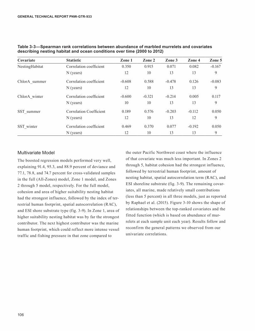
106
GENERAL TECHNICAL REPORT PNW-GTR-933
Multivariate Model The boosted regression models performed very well, explaining 91.4, 95.3, and 88.9 percent of deviance and 77.1, 78.8, and 74.7 percent for cross-validated samples in the full (All-Zones) model, Zone 1 model, and Zones 2 through 5 model, respectively. For the full model, cohesion and area of higher suitability nesting habitat had the strongest inf luence, followed by the index of ter-restrial human footprint, spatial autocorrelation (RAC), and ESI shore substrate type (fig. 3-9). In Zone 1, area of higher suitability nesting habitat was by far the strongest contributor. The next highest contributor was the marine human footprint, which could ref lect more intense vessel traffic and fishing pressure in that zone compared to
the outer Pacific Northwest coast where the inf luence of that covariate was much less important. In Zones 2 through 5, habitat cohesion had the strongest inf luence, followed by terrestrial human footprint, amount of nesting habitat, spatial autocorrelation term (RAC), and ESI shoreline substrate (fig. 3-9). The remaining covar-iates, all marine, made relatively small contributions (less than 5 percent) in all three models, just as reported by Raphael et al. (2015). Figure 3-10 shows the shape of relationships between the top-ranked covariates and the fitted function (which is based on abundance of mur-relets at each sample unit each year). Results follow and reconfirm the general patterns we observed from our univariate correlations.
Table 3-3—Spearman rank correlations between abundance of marbled murrelets and covariates describing nesting habitat and ocean conditions over time (2000 to 2012)
Covariate Statistic Zone 1 Zone 2 Zone 3 Zone 4 Zone 5NestingHabitat Correlation coefficient 0.350 0.915 0.071 0.082 -0.167
N (years) 12 10 13 13 9
ChlorA_summer Correlation coefficient -0.608 0.588 -0.478 0.126 -0.083N (years) 12 10 13 13 9
ChlorA_winter Correlation coefficient -0.600 -0.321 -0.214 0.005 0.117N (years) 10 10 13 13 9
SST_summer Correlation Coefficient 0.189 0.576 -0.203 -0.112 0.050N (years) 12 10 13 12 9
SST_winter Correlation coefficient 0.469 0.370 0.077 -0.192 0.050N (years) 12 10 13 13 9

107
Status and Trend of Marbled Murrelet Populations and Nesting Habitat
##
##
##
##
##
##
##
## ##
##
##
##
##
##
## ##
##
##
##
##
##
##
###
##
##
##
##
##
##
##
##
##
##
##
##
##
##
##
##
##
##
##
##
##
##
##
##
##
##
##
##
##
##
##
##
##
##
##
##
##
##
##
##
##
##
##
##
##
#
##
#
##
#
##
##
##
#
## ##
#
##
##
##
##
##
#
##
##
##
##
## ## ## ## ## ### WIL5WIL9
2.2.12
3.1.1
CR4CR9
# Forage fish station
PSU buffers
PSUs
0 10 205km
Figure 3-6—Location of forage fish survey stations (red triangles) offshore of Willapa Bay (WIL), Washington, and the Columbia River (CR), Oregon. The primary sampling units (PSU) where murrelet at-sea surveys were conducted are boxed in red. The outer black dashed line represents the 20-km buffer used to calculate sea surface temperature and chlorophyll A concentration.

108
GENERAL TECHNICAL REPORT PNW-GTR-933
Figure 3-7—Comparison of trends in forage fish abundance and marbled murrelet abundance in waters near Willapa Bay, Washington (Stratum 2.2) and south of the Columbia River mouth, Oregon (Stratum 3.1), years 2003 to 2011. Years presented are those for which forage fish abundance data were available.
1614121086420
SST
Sea surface temperature
Oceanic Niño Index Pacific Decadal Oscillation Index
Chlorophyll A
WinterSummer
Year20
0220
0320
0420
0520
0820
0920
1020
11
Year
2006
2007
14121086420
Chl
orA
Year
WinterSummer
2.01.51.00.5
00.5
-1.0-1.5-2.0
ON
I
2.52.01.51.00.5
00.5
-1.0-1.5-2.0
PDO
WinterSummer
2002
2003
2004
2005
2008
2009
2010
2011
2006
2007
2005
Year20
0220
0320
0420
0520
0820
0920
1020
1120
0620
07
2002
2003
2004
2005
2008
2009
2010
2011
2006
2007
2002
2003
2004
2005
2008
2009
2010
2011
2006
2007
WinterSummer
A B
C D
Figure 3-8—(A) Sea surface temperature (SST); (B) chlorophyll A concentration (ChlorA); (C) Oceanic Niño Index (ON); and (D) Pacific Decadal Oscillation (PDO) trends in winter (blue line) and summer (orange line) from 2003 through 2011. SST and ChlorA values were based on data from zones proximate to the forage fish sampling stations in figure 3-6.
Zone.Stratum 2.2
Zone.Stratum 3.1Zone.Stratum 2.2
Zone.Stratum 3.1
Mar
bled
mur
rele
t abu
ndan
ce
Marbled murrelet trend Forage fish trend
Tota
l for
age
fish
Year Year2002
1,600
1,400
1,200
1,000
800
600
400
200
0
180,000
160,000
140,000
120,000
100,000
80,000
60,000
40,000
20,000
02003 2004 2005 2006 2007 2008 201120102009 2002 2003 2004 2005 2006 2007 2008 201120102009

109
Status and Trend of Marbled Murrelet Populations and Nesting Habitat
0 10 20 30 40 50 60
RAC
ONI_winter
ESI ShoreType
ONI_summer
ForagingArea
DistToMajorRiver
Depth
PDO_winter
SST_winter
ChlorA_winter
PDO_summer
ChlorA_summer
SST_summer
TerrHumanFoot
NestHabitatCohesion
MarHumanFoot
NestingHabitat
Percentage of contribution
Varia
ble
PSU Scale
All zonesZone 1Zones 2–5
Figure 3-9—Relative influence of marine and terrestrial covariates in boosted regression models of marbled murrelet abundance in 20-km sample units within all zones, within Puget Sound (Zone 1) and along the Pacific Northwest Coast (Zones 2 through 5). See table 3-1 for information about each covariate, except for the residual autocovariate (RAC), which is described in the “Methods” section of chapter 3.
110
GENERAL TECHNICAL REPORT PNW-GTR-933
Figure 3-10—Response curves (fitted function based on marbled murrelet abundance) for the top five covariates (based on contribution to fitted models) depicted in figure 3-9. Models are based on all sample units (left column), sample units in Puget Sound only (Zone 1, center column), and sample units from the outer coast (Zones 2 through 5, right column). See table 3-1 for information about each covariate, except for the residual autocovariate (RAC), which is described in the “Methods” section of chapter 3.
111
Status and Trend of Marbled Murrelet Populations and Nesting Habitat
DiscussionSpatial VariationThe univariate correlations we observed between murrelet abundance and terrestrial or marine factors suggest that terrestrial factors had somewhat stronger relationships, but that marine factors might be responsi-ble for some of the unexplained variation. Although the correlations we observed do not establish a cause-effect relationship, they suggest that proximity of higher suitability nesting habitat inf luences the number of murrelets that occur in the ocean adjacent to that habitat during the breeding season. If true, the amount and pattern of higher suitability nesting habitat might set the carrying capacity for murrelets and that, in turn, would suggest that management focused on conserving and restoring murrelet nesting habitat will contribute to murrelet conservation.
We conclude from these correlations that, among individual variables, the amount and pattern of higher suit-ability nesting habitat seems to have the strongest influence on murrelet abundance at the sampling stratum scale. This information fits with our knowledge about the ecology of the murrelet and the need for nesting birds to remain near nesting habitat (Burger and Waterhouse 2009). With the exception of marine human footprint, none of the marine variables we were able to measure appear to be strongly correlated with murrelet abundance. We caution though, that these results do not mean that the marine environment is not important to murrelets. The fact that our set of marine variables do not correlate with spatial trends in murrelet abundance could be the result of a lack of relationship or because our chosen set of marine variables or their scaling poorly represent aspects of the marine environment impor-tant to murrelets.
Temporal VariationWe found that annual variation in murrelet numbers is more strongly correlated with trend in amount of nesting habitat than trend in ocean indicators. The lack of a consistent relationship between ocean factors and murrelet populations is somewhat surprising. We know that forage fish are the primary food resource for marbled murrelets, particularly
during the breeding season (Nelson 1997). Other research suggests that murrelets change their foraging patterns in response to oceanographic changes (Peery et al. 2009). The fact that we did not see a relationship between ocean pro-ductivity and murrelet populations, may be caused, in part, by our use of indirect measures of productivity (chlorophyll A and SST) as surrogates of murrelet prey populations in our analyses.
For the limited portion of our study where temporal trend in forage fish abundance was available, we did observe a positive relationship between fish abundance and murrelet density over time. This potential relationship with forage fish is not surprising given the often strong positive relationship between forage fish abundance and the abundance of fish-eating birds (e.g., Durant et al. 2009, Furness and Tasker 2000). Murrelets likely evolved in an environment that experienced considerable environmental variability that, in turn, led to fluctuations in prey abun-dance and distribution. However, chronic food scarcity can compromise long-term breeding success (Cury et al. 2011) and can also reduce adult survival in seabirds (Kitaysky et al. 2010). Long-term changes in survival and fecundity would lead to changes in the murrelet population trajectory. There is some information indicating long-term decline in murrelet diet quality in portions of its range (Becker and Beissinger 2006, Gutowsky et al. 2009, Norris et al. 2007), and effects of prey changes on murrelet reproductive success (Becker et al. 2007). Consequently, because of this potential relationship between murrelets and their prey, we recommend attempting to gain a better understanding of the relationship between critical murrelet prey resources and murrelet populations.
Our results indicate that sea surface temperature and chlorophyll A concentration may influence year-to-year changes in murrelet abundance but in a more complex man-ner than our preliminary correlations could detect, at least in zones 1, 2, and 3. The signs of marine correlations did not match our expectations in zones 1 and 3. We expected a positive correlation with chlorophyll concentration and murrelet abundance because we hypothesized that higher concentration of chlorophyll would indicate higher pro-ductivity and hence better foraging conditions and greater
112
GENERAL TECHNICAL REPORT PNW-GTR-933
numbers of murrelets. Instead, we found negative cor-relations in these two zones. Marine productivity in Zone 1 may be driven more by tidal flow, currents, freshwater inputs, and estuaries than upwelling, which may explain the unexpected results in that zone. Zone 3, however, resides in an upwelling system (part of the California Current System) and we are unable to explain the negative correla-tion in that zone. It is probable that our scale or time-frame in these correlation analyses did not capture effects of the marine productivity parameters on murrelet abundance in Zone 3. In addition, forage fish are likely to move some-what independently of chlorophyll A distributions, so this isn’t necessarily surprising given that marbled murrelets are really using habitat that is quite inshore compared to where the majority of upwelling effects are measured (e.g., upwelling-driving chlorophyll A dynamics close to shore where most murrelets occur may not have been accurately captured by the chlorophyll and SST covariates).
Population responses by marbled murrelets to either marine or terrestrial factors are confounded by the mur-relet’s long life span, with an estimated generation time of 10 years (Burger 2002, McShane et al. 2004), and low annual reproductive output. Consequently, there is likely to be a lag between seasonal changes in marine factors (unless they are very dramatic changes reducing murrelet survival) and changes in murrelet populations. Interestingly, there seems to be a decline in murrelet abundance and distribution in response to contemporaneous loss of nesting habitat. One would expect a long-lived species like the murrelet to exhibit a lag in population response to declining habitat; birds would persist in the marine environment until they eventu-ally die. Strong (2003), for example, suggested that declines observed in the 1990s along the Oregon coast might have resulted from losses of habitat stemming from logging in the 1980s or earlier. It is possible that murrelets might move out of an area adjacent to nesting habitat once that habitat is lost and that could explain the relationships we observed, but we have no direct evidence to support that possibility.
Despite the lack of a strong link between the PDO/ENSO phase and sea surface temperature, chlorophyll A, or forage fish abundance, we still observed a strong correlation between forage fish and marbled murrelet abundance in
these same locations (fig. 3-7). Moreover, the decrease in murrelet and forage fish abundance prior to 2007–2008 fol-lowed by an increase after 2007–2008 corresponds to a shift from a warm to cool phase of the PDO. This correlation is consistent with the observation that abundance of other diving seabirds in the California Current System is sensitive to the PDO phase (Ainley and Hyrenbach 2010).
Multivariate ModelWhen we considered the combined influence of both marine and terrestrial influences on the spatial and temporal abun-dance of murrelets, amount and pattern of higher suitability nesting habitat seemed to have the greatest contribution in explaining variation in murrelet abundance within our study area. We found, however, that human influences, both marine (Zone 1) and terrestrial (Zones 2 through 5) were also important. These results reinforce the idea that forest habitat features are limiting factors in murrelet abundance and recovery, but this hypothesis will require further investigation to establish cause-effect relationships.
Effects of ClimateMurrelet nesting habitat and foraging success along the Pacific coast are sensitive to climate variability (Becker et al. 2007), and climate may be contributing to the trends we have observed in murrelet abundance. The trend toward warmer, drier summers along the Pacific coast has favored increased fire frequency and intensity (Littell et al. 2009). This change may be contributing to nesting habitat loss by fire. Although timber harvest was the leading cause of nesting habitat loss on nonfederal lands and all lands combined, more than 60 percent of the habitat losses on federal lands rangewide from 1993 to 2012 were due to wildfire (owing mostly to one fire event, the 2002 Biscuit Fire in southwestern Oregon) (table 2-12). Drier summers also reduce epiphyte growth on branches, thereby degrading the suitability of platforms for nesting (Malt and Lank 2007). During winter, the trend toward increased winter precipitation and more severe storm events has increased the frequency of flooding, landslides, and windthrow (Dale et al. 2001). Warmer winter temperatures and drought stress have also increased the prevalence of tree insect and disease outbreaks. Together, climate-influenced
113
Status and Trend of Marbled Murrelet Populations and Nesting Habitat
factors (wildfire, insects/disease, and natural disturbances) contributed to the rangewide loss of nearly 27,000 ac of higher suitability nesting habitat between 1993 and 2012, compared to losses of less than 8,000 ac from timber harvest on federal lands (table 2-12). Climate change may already be decreasing the quality and quantity of marbled murrelet nesting habitat, and projections for continuation or even acceleration of current climate trends raises the potential for even greater impacts in the future.
In addition to influencing the quality and abundance of nesting habitat, climate variability also has a profound influence on the foraging success of seabirds, including the marbled murrelet (Grémillet and Boulinier 2009). The Cali-fornia Current System, encompassing the entire U.S. Pacific coast (including zones 2 through 5 but excluding inland marine waters such as zone 1), has experienced a warming trend over the past 50 years. This warming is driving a shift from cool, productive sub-arctic ocean conditions toward a warm subtropical marine environment that is less productive (Di Lorenzo et al. 2005). On top of this long-term warming trend, two other sources of climate variability in the Pacific Ocean exert a strong influence on the productivity of coastal waters where the murrelet forages. The El Niño Southern Oscillation (ENSO) is a pattern of sea surface temperature anomalies in the equatorial Pacific that occurs over shorter time scales (every 3 to 7 years and lasting 9 to 18 months (Mestas-Nunez and Miller 2006). During the warm phase (El Niño), upwelling is weaker and sea surface temperature is warmer in the California Current System. Conversely, the cool phase (La Niña) is associated with greater upwelling and cooler sea surface temperature. These shifts in the intensity of upwelling influence nutrient availability in coastal waters, and therefore ENSO phases have profound effects on primary productivity depending on their intensity, with cascading effects at higher trophic levels (Thayer and Sydeman 2007). El Niño events have been associated with poor seabird survival and recruitment throughout the eastern Pacific (Bertram et al. 2005, Hodder and Graybill 1985). At longer time scales (15 to 30 years), the Pacific Decadal Oscillation (PDO) reflects a pattern of sea surface temperature anomalies in the north Pacific (Mestas-Nunez and Miller 2006). Similar to the ENSO cycle, the warm
(positive) phase of the PDO results in weak upwelling in the California Current System and warmer sea surface tempera-ture, while a negative PDO drives strong upwelling and cool sea surface temperature (Mantua et al. 1997). The effects of the ENSO and PDO cycles on upwelling, sea surface tem-perature, and primary productivity are additive. However, some species respond more strongly to either the ENSO or PDO phases, but not both (Black et al. 2011, Sydeman et al. 2009). In addition, the local effect of these broad regional ocean trends is highly modified by undersea topography (which affects the strength and pattern of upwelling), complex trophic interactions, species migrations tracking suitable water temperatures and prey, and food web impacts from commercial fisheries harvest (Doney et al. 2012).
Management Implications Our finding that amount and distribution of higher suit-ability nesting habitat are the primary factors influencing abundance and trend of murrelet populations suggests that land managers should focus particular attention on forest practices that will conserve and restore that habitat. Maintaining the system of late-successional reserves contin-ues to be critical to conservation and restoration of marbled murrelet nesting habitat on federal lands. But even on those reserved lands there are risks to murrelet habitat. Fire and other natural disturbances are already the main cause of nesting habitat loss on federal lands. As described above, climate changes will likely result in loss of existing murrelet habitat owing to increased fire frequency and severity along with increased severity of storms resulting in increased windthrow. During the first 20 years of the NWFP, we documented fire as the main cause of nesting habitat loss on federal lands. Given this finding, predictions of increased fire risk in the future, and the value of higher suitability nesting habitat, which takes a long time to replace, man-agement plans may want to prioritize protection of nesting habitat in reserves, including NWFP late-successional reserves, wilderness, and National Parks.
In chapter 2, we found that a relatively high proportion (typically two-thirds or more) of suitable nesting habitat occurs as small patches (lacking interior forest conditions that are more than 90 m from a patch edge) or as edges of

114
GENERAL TECHNICAL REPORT PNW-GTR-933
larger habitat patches. In this chapter, we found that nesting habitat cohesion, which is the inverse of habitat fragmenta-tion, is a strong predictor of murrelet abundance and trends. This result is not surprising because murrelets prefer larger patches, which also tend to have fewer nest predators (Malt and Lank 2007, Raphael et al. 2002). A key feature of the NWFP is a network of late-successional reserves that have the management objective of protecting and enhancing late-successional forest ecosystems, which serve as habitat for late-successional forest species, including the murrelet. These reserves contain both older and younger forests, and over time, as more mature habitat develops around existing older forest in reserves, patch size should increase, and fragmentation and the prevalence of edges should decrease within reserves. However, it can take many decades for murrelet nesting habitat to develop, and in the short term, protection of existing habitat will continue to be critical to minimize habitat losses, both within and outside of late-successional reserves.
Near-term murrelet conservation should also consider habitat loss caused by windthrow. Windthrow is a natural phenomenon and an important process in coastal forests of the Pacific Northwest, but it can be highly influenced by human activities. Clearcut or heavy thinning harvests can increase the amount of windthrow on the landscape dramatically. This effect depends on complex interactions between biotic (e.g., forest age and condition) and abiotic (e.g., slope and aspect) factors operating at different spatial and temporal scales (Sinton et al. 2000). Portions of forests can also be lost to windthrow after lighter thinning, but the magnitude of the effect depends on factors including topography and tree height-to-diameter ratios (Harrington et al. 2005, Roberts et al. 2007, Wilson and Puettmann 2007). Thus, thinning operations may accelerate the creation of forest conditions suitable to murrelet nesting in the long term (e.g., Maguire et al. 1994), but have short term negative impacts to murrelets to consider in management decisions (McShane et al. 2004).
Forest practices, natural forest disturbance, and the interaction between these factors can increase the amount of forest edge. Increased edge resulting from forest fragmentation appears to have negative effects on mur-
relets. Malt and Lank (2007) found that murrelet nest sites at timber harvest edges had lower moss abundance than interior and natural-edge nest sites (stream corridors and avalanche chutes) owing to stronger winds, higher temper-ature variability, and lower moisture retention. Moss is an important nest substrate on large branches for murrelets in much of the NWFP area, therefore management actions adjacent to suitable murrelet nesting habitat can have implications for murrelets. Another negative impact to murrelets associated with edges, especially those that occur between clearcuts or large openings and forests, is increased nest depredation rates (Marzluff and Neatherlin 2006, Marzluff et al. 2004, Masselink 2001). This is especially true when edges are near human development such as campgrounds (Marzluff and Neatherlin 2006) or include berry-producing plants such as elderberry (Sam-bucus sp.) (Masselink 2001).
One conservation measure that is commonly used to minimize negative effects of forest edges is to provide forested buffers (USFWS 1997). The murrelet recovery plan includes as a short-term recovery action maintaining and enhancing buffer habitat around occupied nesting habitat, and suggests minimum buffer widths of 300 to 600 ft in this situation (USFWS 1997). Buffers around suitable nesting habitat (whether determined to be occupied or not) would help reduce fragmentation, risk of windthrow loss, and potentially reduce nest predation risk (USFWS 1997). Buffers are particularly important in the near term while larger blocks of habitat develop on reserved lands. The details of such buffers are beyond the scope of this report. However, if not already accomplished, development and implementation of forest man-agement practices that protect (short term) and develop (long term) suitable murrelet nesting habitat on NWFP lands within the murrelet range would be beneficial. For such practices, minimizing short-term impacts, such as by avoiding harvest of suitable nesting habitat, providing buffers around suitable nesting habitat to minimize edge effects of management actions (such as from thinning or clearcuts), and minimizing fragmentation of suitable habitat, will likely improve the status of this threatened species.
As described in chapter 2, a substantial amount of suitable nesting habitat occurs on state and private lands.

115
Status and Trend of Marbled Murrelet Populations and Nesting Habitat
The loss of habitat on those lands is occurring at a much more rapid rate than on federal lands. Because of the strong relationship between murrelet populations and nesting habitat and because recovery of murrelet populations will likely require contributions of nesting habitat on state and private lands, at least in the short term (as discussed in the murrelet recovery plan), there is a need for incentives for private forest landowners to avoid fragmentation and loss of high-quality nesting habitat and to maintain blocks of interior nesting habitat on the landscape as well as buffers adjacent to suitable habitat on federal and state lands.
Another conservation measure worthy of additional investigation is the management of potential nest pred-ators. In central California (outside the NWFP area), an aggressive program to deter nest predation has been enacted to try and improve marbled murrelet nesting success (Henry and Peery 2010). Similar programs in fragmented or in suitable nesting habitat near human populations or campgrounds may prove beneficial. We emphasize that this is a conservation measure of which we have little understanding as to its population-level effectiveness. Consequently, predator management actions should be conducted in a research framework so that their effectiveness can be evaluated.
Summary ConclusionsOur most prominent finding in combining results of chapters 1 and 2 into multivariate models is the strong relationship between stands of cohesive and higher suit-ability nesting habitat and the distribution and trends of murrelets at sea. Areas of greatest habitat loss over the time series tended to be the areas with greatest murrelet decline. Habitat loss occurred in all zones, with greater loss documented in Washington, where the steepest declines in murrelet populations occurred. Though we found no prom-inent effects of marine factors on murrelet distribution and population trend in this analysis, our analyses were limited by the unavailability of direct measures of murrelet prey abundance, and selection of appropriate marine parameters and temporal frames remains a complex problem that war-rants further investigation. We did a preliminary analysis on a number of factors that did not appear to have direct links
to murrelet abundance, but we did find what appears to be a promising relationship between temporal trends in murrelet abundance with forage fish abundance, and that this may indicate an important marine causal factor in nesting success that remains to be quantified (e.g., Ainley et al. 2015). Incorporating fish sampling with ongoing population surveys at sea would be a good next step to further explore this relationship.
Several points bear repeating: (1) loss of higher suitability habitat has been relatively low on federal land compared to nonfederal land since creation of the North-west Forest Plan; (2) marbled murrelet declines are not related to the small loss of higher suitability habitat on federal lands, but could be related to the lack of buffers and heavy thinning adjacent to murrelet habitat in the late-successional reserves; and (3) there appears to be a strong relationship between murrelet population declines and the large loss of higher suitability habitat on nonfederal land, especially in Zone 2.
Among the factors we investigated, nesting habitat factors were the best predictors of marbled murrelet population distribution and trends at sea. However, there was unexplained variance, which implies that habitat monitoring alone is not sufficient at this time to predict murrelet population trends. Also, given the breadth of forest types within the study area, the relationship between murrelets numbers and nesting habitat conditions may vary geographically. Therefore, population monitoring continues to be an essential element of measuring the effectiveness of murrelet conservation and restoration efforts, while the monitoring program continues to evaluate predictive models relating murrelet population distribution and trends to terrestrial nesting habitat and marine conditions. The primary hypothesis emerging from our work is that marbled murrelet distribution and trend in the breeding season is largely determined by amount and trend of suitable nesting habitat. If this is true, and if amounts of habitat increase in the future as currently unsuitable habitat matures within federal reserves, then we should see a concomitant increase in murrelet population size. This will be an important test of our hypothesis, and continued monitoring is needed to complete this test.
116
GENERAL TECHNICAL REPORT PNW-GTR-933
AcknowledgmentsThis work was conducted under the auspices of the North-west Forest Plan Effectiveness Monitoring Program, and we are indebted to that program for support. We thank the U.S. Fish and Wildlife Service, the Washington Depart-ment of Fish and Wildlife, and the Forest Service’s Pacific Northwest Research Station for financial support. We thank Robert Emmett and John Fields of NOAA Fisheries for forage fish data. We also thank Ashley Steel, Mark Huff, Douglas Bertram, and Jeanette Zamon for reviews of an earlier draft. The findings and conclusions in this article are those of the authors and do not necessarily represent the views of the U.S. Fish and Wildlife Service.
ReferencesAinley, D.G.; Adams, P.B.; Jahncke, J. 2015. California
current system: predators and the preyscape. Journal of Marine Systems. 146: 1–2.
Ainley, D.G.; Hyrenbach, D.K. 2010. Top-down and bottom-up factors affecting seabird population trends in the California current system (1985–2006). Progress in Oceanography. 84: 242–254.
Becker, B.H.; Beissinger, S.R. 2006. Centennial decline in the trophic level of an endangered seabird after fisheries decline. Conservation Biology. 20: 470–479.
Becker, B.H.; Peery, M.Z.; Beissinger, S.R. 2007. Ocean climate and prey availability affect the trophic level and reproductive success of the marbled murrelet, an endangered seabird. Marine Ecology Progress Series. 329: 267–279.
Bertram, D.F.; Harfenist, A.; Smith, B.D. 2005. Ocean climate and El Niño impacts on survival of Cassin’s Auklets from upwelling and downwelling domains of British Columbia. Canadian Journal of Fisheries and Aquatic Sciences. 62: 2841–2853.
Black, B.A.; Schroeder, I.D.; Sydeman, W.J.; Bograd, S.J.; Wells, B.K.; Schwing, F.B. 2011. Winter and summer upwelling modes and their biological importance in the California Current Ecosystem. Global Change Biology. 17: 2536–2545.
Burger, A.E. 2002. Conservation assessment of marbled murrelets in British Columbia, a review of the biology, populations, habitat associations, and conservation. Technical Report 387. Delta, British Columbia, Canada: Canadian Wildlife Service. 194 p.
Burger, A.E.; Waterhouse, F.L. 2009. Relationships between habitat area, habitat quality, and populations of nesting marbled murrelets. BC Journal of Ecosystems and Management. 10: 101–112.
Crase, B.; Liedloff, A.C.; Wintle, B.A. 2012. A new method for dealing with residual spatial autocorrelation in species distribution models. Ecography. 35: 879–888.
Cury, P.M.; Boyd, I.L.; Bonhommeau, S.; Anker-Nilssen T. and others. 2011. Global seabird response to forage fish depletion one-third for the birds. Science. 334: 1703–1706.
Dale, V. H.; Joyce, L.A.; McNulty, S.; Neilson, R.P.; Ayres, M.P.; Flannigan, M.D.; Hanson, P.J.; Irland, L.C.; Lugo, A.E.; Peterson, C.J.; Simberloff, D.; Swanson, F.J.; Stocks, B.J.; Wotton, M. 2001. Climate change and forest disturbances: climate change can affect forests by altering the frequency, intensity, duration, and timing of fire, drought, introduced species, insect and pathogen outbreaks, hurricanes, windstorms, ice storms, or landslides. BioScience. 51: 723–734.
Di Lorenzo, E.; Miller, A. J.; Schneider, N.; McWilliams, J. C. 2005. The warming of the California Current System: dynamics and ecosystem implications. Journal of Physical Oceanography. 35: 336–362.
Doney, S.C.; Ruckelshaus, M.; Duffy, J.E.; Barry, J.P.; Chan, F.; English, C.A.; Talley, L.D. 2012. Climate change impacts on marine ecosystems. Annual Review of Marine Science. 4: 11–37.
117
Status and Trend of Marbled Murrelet Populations and Nesting Habitat
Durant J.M.; Hjermann, D.Ø.; Frederiksen, M.; Charrassin, J.B.; Le Maho, Y.; Sabarros, P.S.; Crawford, R.J.M.; Stenseth, N.C. 2009. Pros and cons of using seabirds as ecological indicators. Climate Research. 39: 115–129.
Elith J.; Leathwick, J.R.; Hastie, T. 2008. A working guide to boosted regression trees. Journal of Animal Ecology. 77: 802–813.
Emmett, R.L. 2014. Personal communication. Research scientist, National Oceanographic and Atmospheric Administration, Northwest Fisheries Science Center, 2030 SE Marine Science Drive. Newport, OR 97365. [email protected].
Forests, Lands, and Natural Resources Operations [FLNRO]. 2012. Old growth management areas. Victoria, British Columbia, Canada: Government of British Columbia. https://apps.gov.bc.ca/pub/geometadata/home.do. (22 May 2012).
Forest Ecosystem Management Assessment Team [FEMAT]. 1993. Forest ecosystem management: an ecological, economic, and social assessment. Portland, OR: U.S. Department of Agriculture; U.S. Department of the Interior [and others]. [Irregular pagination].
Furness, R.W.; Tasker, M.L. 2000. Seabird-fishery interactions: quantifying the sensitivity of seabirds to reductions in sandeel abundance, and identification of key areas for sensitive seabirds in the North Sea. Marine Ecology Progress Series. 202: 253–264.
Grémillet, D.; Boulinier, T. 2009. Spatial ecology and conservation of seabirds facing global climate change: a review. Marine Ecology Progress Series. 391: 121–137.
Gutowsky S.; Janssen, M.H.; Arcese, P.; Kyser, T.K. and others. 2009. Concurrent declines in nestling diet quality and reproductive success of a threatened seabird over 150 years. Endangered Species Research. 9: 247–254.
Halpern, B.S.; Walbridge, S.; Selkoe, K.A.; Kappel, C.V.; Micheli, F.; D’Agrosa, C.; Bruno, J.F.; Kasey K.S.; Ebert, C.; Fox, H.E.; Fujita, R.; Heinemann, D.; Lenihan, H.S.; Madin, E.M.P.; Perry, M.T.; Selig, E.R.; Spalding, M.; Steneck, R.; Watson R. 2008. A global map of human impact on marine ecosystems. Science. 319: 948–952.
Harrington, C.A.; Roberts, S.D.; Brodie, L.C. 2005. Tree and understory responses to variable density thinning in western Washington. In: Peterson, C.E.; Maguire, D.A., eds. Balancing ecosystem values. Gen. Tech. Rep. PNW GTR-635. Portland, OR: U.S. Department of Agriculture, Forest Service, Pacific Northwest Research Station: 97–106.
Hébert, P.N.; Golightly, R.T. 2008. At-sea distribution and movements of nesting and non-nesting marbled murrelets Brachyramphus marmoratus in Northern California. Marine Ornithology. 36: 99–105.
Henry, R.M.; Peery, M.Z. 2010. Recovering marbled murrelets via corvid management: A population viability analysis approach. Biological Conservation. 143: 2414–2424.
Hijmans, R. J.; Phillips, S.J.; Leathwick, J.R.; Elith J. 2012. R package ‘dismo’: Species distribution modeling. Version 0.7-23.
Hodder, J.; Graybill, M.R. 1985. Reproduction and survival of seabirds in Oregon during the 1982–1983 El Niño. Condor. 87: 535–541.
JISAO 2012. PDO index. Seattle, WA: University of Washington, Joint Institute for the Study of the Atmosphere and Ocean. http://jisao.washington.edu/pdo/PDO.latest. (15 January 2012).
Kitaysky, A.S.; Piatt, J.F.; Hatch; S.A.; Kitaiskaia, A.V.; Benowitz-Fredericks, Z.M., and others. 2010. Food availability and population processes: severity of nutritional stress during reproduction predicts survival of long-lived seabirds. Functional Ecology. 24: 625–637.
118
GENERAL TECHNICAL REPORT PNW-GTR-933
Leu, M.; Hanser, S.E.; Knick, S.T. 2008. The human footprint in the west: a large-scale analysis of anthropogenic impacts. Ecological Applications. 18: 1119–1139.
Littell, J.S.; McKenzie D; Peterson D.L.; Westerling, A.L. 2009. Climate and wildfire area burned in western U.S. ecoprovinces, 1916–2003. Ecological Applications. 19: 1003–1021.
Madsen, S.; Evans-Mack, D.; Hamer, T.; Henson, P.; Miller, S.; Nelson, S.K.; Roby, D.; Stapanian M. 1999. Marbled murrelet effectiveness monitoring plan for the Northwest Forest Plan. Gen. Tech. Rep. PNW-GTR-439. U.S. Department of Agriculture, Forest Service, Pacific Northwest Research Station, Portland, OR. 51 p.
Maguire, D.A.; Moeur, M.; Bennett, W.S. 1994. Models for describing basal diameter and vertical distribution of primary branches in young Douglas-fir. Forest Ecology and Management. 63: 23–55
Malt, J.; Lank, D. 2007. Temporal dynamics of edge effects on nest predation risk for the marbled murrelet. Biological Conservation. 140: 160–173.
Mantua, N.J.; Hare, S.R.; Zhang, Y.; Wallace, J.M.; Francis, R.C. 1997. A Pacific interdecadal climate oscillation with impacts on salmon production. Bulletin of the American Meteorological Society. 78: 1069–1079.
Marzluff, J.M.; Millspaugh, J.J.; Hurvitz, P.; Handcock, M.S. 2004. Relating resources to a probabilistic measure of space use: forest fragments and Steller’s Jays. Ecology. 85: 1411–1427.
Marzluff, J. M.; Neatherlin, E. 2006. Corvid responses to human settlements and campgrounds: causes, consequences, and challenges for conservation. Biological Conservation. 130: 301–314.
Masselink, M.N.M. 2001. Responses of Steller’s Jays to forest fragmentation on southwest Vancouver Island and potential impacts on marbled murrelets. Victoria, BC: University of Victoria, Department of Biology: 138 p. M.S. thesis.
McGarigal, K.; Cushman, S.A.; Ene, E. 2012. FRAGSTATS v4: Spatial pattern analysis program for categorical and continuous maps. Amherst, MA: University of Massachusetts, Landscape Ecology Lab. http://www.umass.edu/landeco/research/fragstats/fragstats.html. (1 July 2015).
McShane, C.; Hamer, T.; Carter, H.R.; Swartzman, G.; Friesen, V.; Ainley, D.; Tressler, G.; Nelson, S.K.; Burger, A.; Spear, L.; Mohagen, T.; Martin, R.; Henkel, L.; Prindle, K.; Strong, C.; Keany, J. 2004. Evaluation report for the 5-year status review of the marbled murrelet in Washington, Oregon, and California. Seattle, WA: EDAW Inc. http://www.fws.gov/arcata/es/birds/MM/documents/mm5yr_rpt_final_web.pdf. (1 July 2015).
Mestas-Nuñez, A. M; Miller, A. J. 2006. Interdecadal variability and climate change in the eastern tropical Pacific: a review. Progress in Oceanography. 69: 267–284.
NASA Earth Observations Portal. 2012. http://neo.sci.gsfc.nasa.gov/?pg=2&datasetId=MY1DMM_CHLORA&group=12. (1 July 2015).
Nelson, S.K. 1997. Marbled murrelet (Brachyramphus marmoratus). In: Poole, A.; Gill, F., eds. Birds of North America, No. 276. Philadelphia, PA: Academy of Natural Sciences; Washington, DC: American Ornithologists Union. 32 p.
Norris, D.R.; Arcese, P.; Preikshot, D.; Bertram, D.F.; Kyser, T.K. 2007. Diet reconstruction and historic population dynamics in a threatened seabird. Journal of Applied Ecology. 44: 875–884.

119
Status and Trend of Marbled Murrelet Populations and Nesting Habitat
Peery, M.Z.; Newman, S.H.; Storlazzi, C.D.; Beissinger, S.R. 2009. Meeting reproductive demands in a dynamic upwelling system: Foraging strategies of a pursuit-diving seabird, the marbled murrelet. Condor. 111: 120–134.
R Development Core Team. 2012. R: a language and environment for statistical computing. Vienna, Austria: R Foundation for Statistical Computing. http://www.R-project.org. (1 July 2015).Raphael, M.G. 2006. Conservation of the Marbled Murrelet under the Northwest Forest Plan. Conservation Biology. 20: 297–305.
Raphael, M.G.; Baldwin, J.; Falxa, G.A.; Huff, M.H.; Lance, M.; Miller, S.L.; Pearson, S.F.; Ralph, C.J.; Strong, C.; Thompson, C. 2007. Regional population monitoring of the marbled murrelet: field and analytical methods. Gen. Tech. Rep. PNW-GTR-716. Portland, OR: U.S. Department of Agriculture, Forest Service, Pacific Northwest Research Station. 70 p. http://www.fs.fed.us/pnw/pubs/pnw_gtr716.pdf. (24 June 2015).
Raphael, M.G.; Evans-Mack, D.; Marzluff, J.M.; Luginbuhl, J.M. 2002. Effects of forest fragmentation on populations of the marbled murrelet. Studies in Avian Biology. 25: 221–235.
Raphael, M.G.; Falxa, G.A.; Dugger, K.M.; Galleher, B.M.; Lynch, D.; Miller, S.L.; Nelson, S.K.; Young, R.D. 2011. Status and trend of nesting habitat for the marbled murrelet under the Northwest Forest Plan. Gen. Tech. Rep. PNW-GTR-848. Portland, OR: U.S. Department of Agriculture, Forest Service, Pacific Northwest Research Station. 52 p.
Raphael, M.G.; Shirk, A.J.; Falxa, G.A.; Pearson, S.F. 2015. Habitat associations of marbled murrelets during the nesting season in nearshore waters along the Washington to California coast. Journal of Marine Systems. 146: 17–25.
Roberts, S.D.; Harrington, C.A.; Buermeyer, K.R. 2007. Does variable-density thinning increase wind damage in conifer stands on the Olympic Peninsula? Western Journal of Applied Forestry. 22: 285–296.
Sinton D.S.; Jones, J.A.; Ohmann, J.L.; Swanson, F.J. 2000. Windthrow disturbance, forest composition, and structure in the Bull Run Basin, Oregon. Ecology. 81: 2539–2556.
Strong, C.S. 2003. Decline of the marbled murrelet population on the central Oregon coast during the 1990s. Northwestern Naturalist. 84: 31–37.
Sydeman, W.J.; Mills, K.L.; Santora, J.A.; Thompson, S.A.; Bertram, D.F.; Morgan, K.H.; Wells, B.K.; Hipfner, J.M.; Wolf, S.G. 2009. Seabirds and climate in the California Current—a synthesis of change. CalCOFI Reports. 50: 82–104.
Thayer, J.A.; Sydeman, W.J. 2007. Spatio-temporal variability in prey harvest and reproductive ecology of a piscivorous seabird, Cerorhinka monocerata, in an upwelling system. Marine Ecology Progress Series. 329: 253–265.
Trenberth, K.E. 1997. The definition of El Niño. Bulletin of the American Meteorological Society. 78: 2771–2777.
U.S. Department of Commerce, National Oceanographic and Atmospheric Administration [NOAA]. 2002. Environmental sensitivity index guidelines, version 3.0. NOAA Technical Memorandum NOS ORCA 115. Seattle, WA: Hazardous Materials Response and Assessment Division. 79 p.
U.S. Department of Commerce, National Oceanographic and Atmospheric Administration [NOAA]. 2012a. Cold & warm episodes by season. Camp Springs, MD: NOAA National Centers for Environmental Prediction, Climate Prediction Center. http://www.cpc.ncep.noaa.gov/products/analysis_monitoring/ensostuff/ensoyears.shtml. (15 January 2012).
120
GENERAL TECHNICAL REPORT PNW-GTR-933
U.S. Department of Commerce, National Oceanographic and Atmospheric Administration [NOAA]. 2012b. Ocean ecosystem indicators. Seattle, WA: Northwest Fisheries Science Center, Estuarine and Ocean Ecology Program. http://www.nwfsc.noaa.gov/research/divisions/fe/estuarine/oeip/index.cfm. (1 July 2015).
U.S. Department of the Interior, Fish and Wildlife Service [USFWS]. 1997. Recovery plan for the threatened marbled murrelet (Brachyramphus marmoratus) in Washington, Oregon, and California. Portland, OR. 203 p.
Wilson, D.S.; Puettmann, K.J. 2007. Density management and biodiversity in young Douglas-fir forests: Challenges of managing across scales. Forest Ecology and Management. 246: 123–134.
Zamon, J.E.; Phillips, E.M.; Guy, T.J. 2014. Marine bird aggregations associated with the tidally-driven plume and plume fronts of the Columbia River. Deep Sea Research Part II: Topical Studies in Oceanography. 107: 85–95.
121
Status and Trend of Marbled Murrelet Populations and Nesting Habitat
Appendix 1: Power Analysis
IntroductionBecause one objective of our monitoring is to detect a change over time, it is desirable to have the statistical power to detect a decline in a time frame that allows managers to respond by altering land management strategies. We conducted a new power analysis for this report by using the larger set of available data to determine the sampling design’s power to detect a decline for each conservation zone and for all conservation zones combined. This replaces previous power analyses by Miller et al. (2006) and Falxa et al. (2011), which were based on 2000–2003 and 2001–2009 data, respectively. The reason for conducting this analysis is to assess power associated with a reduced sampling effort from 2014 forward. This assumption reflects a decision among agency managers, discussed below, to reduce sampling frequency to every other year effective in 2014.
MethodsOur method for calculating power combines those described by Hogg and Craig (1995) and Draper and Smith (1998), and used monitoring data from 2001 through 2013.
As noted above, for this power analysis we assumed that conservation zones will be surveyed every other year such that surveys will now be made in even years for two of the conser-vation zones (Conservation Zones 1 and 3), in odd years for Conservation Zones 2 and 4, and every 4 years in Conservation Zone 5. To approximate the power to detect linear trends (in the log of the density) we assumed the full complement of existing surveys up to 2013 for Conservation Zones 2, 4, and 5 and up to 2014 for Conservation Zones 1 and 3. Then we assumed surveys only in every other year except for Conservation Zone 5, for which surveys in every 4 years were considered.
We estimated the power to detect annual rates of population change of 1, 2, 3, 4, and 5 percent. We did this by simulating data from a regression of the surveyed years using the slope associated with annual declines of 1, 2, 3, 4, and 5 percent and the estimated root mean square error from the data collected so far, through 2013. There were 1,000 simulations per conservation zone, annual change, and year combination. The estimated power curves were smoothed in an attempt to obtain more accurate power results by regressing the inverse normal distribution
function of the power estimates and the year. The predicted values were used to display the power curves (fig. A-1).
Results
Figure A-1—The following charts (figs. A-1a through A-1f) represent the power to detect population declines at annual rates of change ranging from 1 to 5 percent. Power estimates assumed the use of data from annual sampling to date (since 2000–2001), and assumes sampling in every other year from 2014 on. The exception is Conservation Zone 5, which is based on only those years actually sampled through 2013, and on sampling every 4 years from 2014 on.
2020 2030 2040 2050 20600
0.2
0.4
0.6
0.8
1.0All zones
Year
Pow
er
A
2020 2030 2040 2050 2060
0
0.2
0.4
0.6
0.8
1.0Zone 1
Year
Pow
er
Annual change-5%-4%-3%-2%-1%
B
122
GENERAL TECHNICAL REPORT PNW-GTR-933
Figure A-1 (continued)—The following charts (figs. A-1a through A-1f) represent the power to detect population declines at annual rates of change ranging from 1 to 5 percent. Power estimates assumed the use of data from annual sampling to date (since 2000–2001), and assumes sampling in every other year from 2014 on. The exception is Conservation Zone 5, which is based on only those years actually sampled through 2013, and on sampling every 4 years from 2014 on.
2020 2030 2040 2050 20600
0.2
0.4
0.6
0.8
1.0
Year
Pow
er
Zone 2C
Annual change-5%-4%-3%-2%-1%
2020 2030 2040 2050 20600
0.2
0.4
0.6
0.8
1.0
Year
Pow
er
Zone 3D
Annual change-5%-4%-3%-2%-1%
2020 2030 2040 2050 20600
0.2
0.4
0.6
0.8
1.0
Year
Pow
er
Zone 4E
Annual change-5%-4%-3%-2%-1%
2020 2030 2040 2050 2060
0
0.2
0.4
0.6
0.8
1.0
Year
Pow
er
Zone 5F
Annual change-5%-4%-3%
-2%-1%
123
Status and Trend of Marbled Murrelet Populations and Nesting Habitat
Power to Detect TrendsOur measure for assessing the effectiveness of the monitor-ing design is its power to detect changes in the mean density and the resulting mean total population of marbled mur-relets over time. Tables A-1 and A-2 present the estimated years when sampling will be sufficient to detect a trend in a population declining at various rates of annual population decrease for two levels of power: 0.80 and 0.95. These power numbers measure the ability of the sampling design to detect a significant trend, if one exists. For example, if we use a power level of 0.80 and for a rate of decline of 3 percent per year, the power analysis results would estimate
the number of years of sampling required to detect a real 3-percent decline, with an 80-percent probability of detect-ing that trend (equals the probability of correctly rejecting the null hypothesis).
For the population of the five conservation zones combined, the power analysis estimated that by 2013 enough years had been sampled to detect an annual decrease of 3 per-cent with greater than 95-percent power, and that an annual decrease of 2 percent could be detected with about 5 more years of sampling (through 2018) at 95-percent power (table A-2). Sampling through 2024 would be required to detect an annual decrease of 1 percent at the scale of the combined
Table A-1—Estimates of the year when 80-percent or greater power will be achieved to detect various rates of annual decrease in the NWFP marbled murrelet population, based on data from surveys starting in 2000/2001
Annual rate of decrease
Conservation ZoneAll 1 2 3 4 5
Year when 80-percent power achievedPercent1 2024 2040 2049 2034 2031 >20592 A 2026 2031 2020 2021 20513 A 2020 2023 A A 20394 A 2016 2019 A A 20315 A A 2017 A A 2027As described in the text, the power analysis assumed that, starting in 2014, Conservation Zones 1 through 4 are sampled every other year and Zone 5 is sampled every 4 years. Reported for all conservation zones combined and by individual conservation zone. An “A” in a cell indicates that this level of power has already been achieved. A decline can have been detected already, even if 80-percent power has not been reached, such as for Conservation Zone 2. See text for details.
Table A-2—This table is similar to table A-1, but reports the year when 95 percent or greater power will be achieved to detect various percentages of annual decrease in the NWFP murrelet population, for all conservation zones combined and by individual zone
Annual rate of decrease
Conservation ZoneAll 1 2 3 4 5
Year when 95-percent power achievedPercent1 2028 2048 2059 2042 2039 >20592 2018 2030 2037 2024 2023 >20593 A 2024 2029 2018 2017 20474 A 2020 2023 A A 20395 A 2016 2021 A A 2035An “A” in a cell indicates that this level of power has already been achieved.
124
GENERAL TECHNICAL REPORT PNW-GTR-933
conservation zones with 80-percent power; sampling through 2028 would increase the power to 95 percent. At the single-conservation-zone scale, the decrease we could detect with monitoring to date differs among the five conservation zones. Power is fairly similar for Conservation Zones 3 and 4 in which sampling to date is sufficient to detect annual decreases of 3 percent or greater with at least 80-percent power, and a decrease of 4 percent or greater with about 95-percent power. In Conservation Zones 1 and 2, where interannual variability has been slightly greater, statistical power is slightly higher for sampling to date, being sufficient by 2017 to detect annual declines since 2001 of 5 percent with 80-percent power (table A-1); we note that a significant decline has already been detected for Conservation Zone 2, at an estimate annual rate of about 7 percent per year. The number of years required to detect a trend is highest for Conservation Zone 5.
ReferencesFalxa, G.; Baldwin, J.; Lynch, D., Miller, S.L.; Nelson,
S.K.; Pearson, S.F.; Raphael, M.G.; Strong, C.; Bloxton, T.; Galleher, B.; Hogoboom, B.; Lance, M.; Young, R. 2011. Marbled murrelet effectiveness monitoring, Northwest Forest Plan: 2009 and 2010 summary report. 26 p. http://www.reo.gov/monitoring/reports/murrelet/mamu_2009-2010_em_annual%20monitoring%20report.pdf. (19 June 2015).
Draper, N.R.; Smith, H. 1998. Applied regression analysis, 3rd ed. New York: John Wiley and Sons. 706 p.
Hogg, R.V.; Craig, A.T. 1995. Introduction to mathematical statistics, 5th ed. Englewood Cliffs, NJ: Prentice-Hall. 564 p.
Miller, S.L; Ralph, C.J.; Raphael, M.G.; Strong, C.; Thompson, C.W.; Baldwin, J.; Huff, M.H.; Falxa, G.A. 2006. At-sea monitoring of marbled murrelet population status and trend in the Northwest Forest Plan area. In: Huff, M.H.; Raphael, M.G.; Miller, S.L.; Nelson, S.K.; Baldwin, J., tech. coords. Northwest Forest Plan—the first 10 years (1994–2003): status and trends of populations and nesting habitat for the marbled murrelet. Gen. Tech. Rep. PNW-GTR-650. Portland, OR: US. Department of Agriculture, Forest Service, Pacific Northwest Research Station: 31–60. Chapter 3.

125
Status and Trend of Marbled Murrelet Populations and Nesting Habitat
Appendix 2: Field Audit Form
Checklist for Field AuditMarbled Murrelet Long-Term Monitoring Surveys
Name of Auditor Date / /
Field Crew (name or location) Survey Vessel
Time Begin End
Was each crewmember observed as a: Survey observer Boat operator
If not, was the observer/navigator configuration different from the previous audit?
Is the track line of the transect:
Being recorded by GPS and downloaded each day?
Paused during forays off the transect line and between segment start and end points?
Did observers:
Scan with greater effort close to the transect line?
Record distances at first detection?
Record all murrelet groups detected, regardless of distance from the line?
Record flying murrelets?
Communicate with each other on groups close to the line?
Alert each other to murrelet groups to minimize missed detections?
Define group size consistent with each other and with protocol definition?
Are distance trials:
Conducted in sets of 5, with all 5 estimates within 15%?
Up to date (completed every 3 days)?
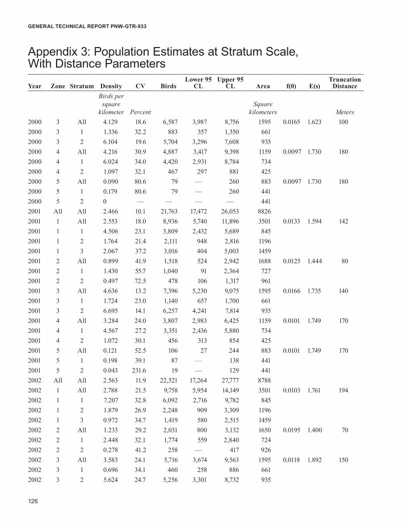
126
GENERAL TECHNICAL REPORT PNW-GTR-933
Appendix 3: Population Estimates at Stratum Scale, With Distance Parameters
Year Zone Stratum Density CV BirdsLower 95
CLUpper 95
CL Area f(0) E(s)Truncation
DistanceBirds per
square kilometer Percent
Square kilometers Meters
2000 3 All 4.129 18.6 6,587 3,987 8,756 1595 0.0165 1.623 1002000 3 1 1.336 32.2 883 357 1,350 6612000 3 2 6.104 19.6 5,704 3,296 7,608 9352000 4 All 4.216 30.9 4,887 3,417 9,398 1159 0.0097 1.730 1802000 4 1 6.024 34.0 4,420 2,931 8,784 7342000 4 2 1.097 32.1 467 297 881 4252000 5 All 0.090 80.6 79 — 260 883 0.0097 1.730 1802000 5 1 0.179 80.6 79 — 260 4412000 5 2 0 — — — — 4412001 All All 2.466 10.1 21,763 17,472 26,053 88262001 1 All 2.553 18.0 8,936 5,740 11,896 3501 0.0133 1.594 1422001 1 1 4.506 23.1 3,809 2,432 5,689 8452001 1 2 1.764 21.4 2,111 948 2,816 11962001 1 3 2.067 37.2 3,016 404 5,003 14592001 2 All 0.899 41.9 1,518 524 2,942 1688 0.0125 1.444 802001 2 1 1.430 55.7 1,040 91 2,364 7272001 2 2 0.497 72.5 478 106 1,317 9612001 3 All 4.636 13.2 7,396 5,230 9,075 1595 0.0166 1.735 1402001 3 1 1.724 23.0 1,140 657 1,700 6612001 3 2 6.695 14.1 6,257 4,241 7,814 9352001 4 All 3.284 24.0 3,807 2,983 6,425 1159 0.0101 1.749 1702001 4 1 4.567 27.2 3,351 2,436 5,880 7342001 4 2 1.072 30.1 456 313 854 4252001 5 All 0.121 52.5 106 27 244 883 0.0101 1.749 1702001 5 1 0.198 39.1 87 — 138 4412001 5 2 0.043 231.6 19 — 129 4412002 All All 2.563 11.9 22,521 17,264 27,777 87882002 1 All 2.788 21.5 9,758 5,954 14,149 3501 0.0103 1.761 1942002 1 1 7.207 32.8 6,092 2,716 9,782 8452002 1 2 1.879 26.9 2,248 909 3,309 11962002 1 3 0.972 34.7 1,419 580 2,515 14592002 2 All 1.233 29.2 2,031 800 3,132 1650 0.0195 1.400 702002 2 1 2.448 32.1 1,774 559 2,840 7242002 2 2 0.278 41.2 258 — 417 9262002 3 All 3.583 24.1 5,716 3,674 9,563 1595 0.0118 1.892 1502002 3 1 0.696 34.1 460 258 886 6612002 3 2 5.624 24.7 5,256 3,301 8,732 935
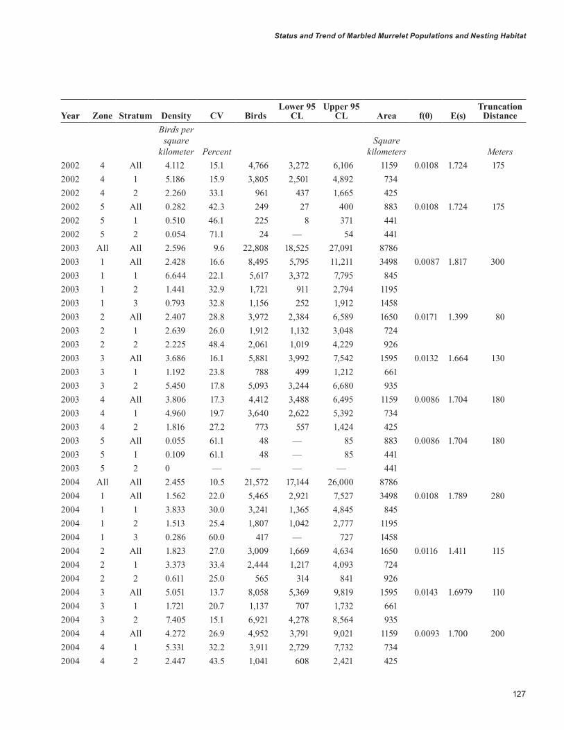
127
Status and Trend of Marbled Murrelet Populations and Nesting Habitat
Year Zone Stratum Density CV BirdsLower 95
CLUpper 95
CL Area f(0) E(s)Truncation
DistanceBirds per
square kilometer Percent
Square kilometers Meters
2002 4 All 4.112 15.1 4,766 3,272 6,106 1159 0.0108 1.724 1752002 4 1 5.186 15.9 3,805 2,501 4,892 7342002 4 2 2.260 33.1 961 437 1,665 4252002 5 All 0.282 42.3 249 27 400 883 0.0108 1.724 1752002 5 1 0.510 46.1 225 8 371 4412002 5 2 0.054 71.1 24 — 54 4412003 All All 2.596 9.6 22,808 18,525 27,091 87862003 1 All 2.428 16.6 8,495 5,795 11,211 3498 0.0087 1.817 3002003 1 1 6.644 22.1 5,617 3,372 7,795 8452003 1 2 1.441 32.9 1,721 911 2,794 11952003 1 3 0.793 32.8 1,156 252 1,912 14582003 2 All 2.407 28.8 3,972 2,384 6,589 1650 0.0171 1.399 802003 2 1 2.639 26.0 1,912 1,132 3,048 7242003 2 2 2.225 48.4 2,061 1,019 4,229 9262003 3 All 3.686 16.1 5,881 3,992 7,542 1595 0.0132 1.664 1302003 3 1 1.192 23.8 788 499 1,212 6612003 3 2 5.450 17.8 5,093 3,244 6,680 9352003 4 All 3.806 17.3 4,412 3,488 6,495 1159 0.0086 1.704 1802003 4 1 4.960 19.7 3,640 2,622 5,392 7342003 4 2 1.816 27.2 773 557 1,424 4252003 5 All 0.055 61.1 48 — 85 883 0.0086 1.704 1802003 5 1 0.109 61.1 48 — 85 4412003 5 2 0 — — — — 4412004 All All 2.455 10.5 21,572 17,144 26,000 87862004 1 All 1.562 22.0 5,465 2,921 7,527 3498 0.0108 1.789 2802004 1 1 3.833 30.0 3,241 1,365 4,845 8452004 1 2 1.513 25.4 1,807 1,042 2,777 11952004 1 3 0.286 60.0 417 — 727 14582004 2 All 1.823 27.0 3,009 1,669 4,634 1650 0.0116 1.411 1152004 2 1 3.373 33.4 2,444 1,217 4,093 7242004 2 2 0.611 25.0 565 314 841 9262004 3 All 5.051 13.7 8,058 5,369 9,819 1595 0.0143 1.6979 1102004 3 1 1.721 20.7 1,137 707 1,732 6612004 3 2 7.405 15.1 6,921 4,278 8,564 9352004 4 All 4.272 26.9 4,952 3,791 9,021 1159 0.0093 1.700 2002004 4 1 5.331 32.2 3,911 2,729 7,732 7342004 4 2 2.447 43.5 1,041 608 2,421 425

128
GENERAL TECHNICAL REPORT PNW-GTR-933
Year Zone Stratum Density CV BirdsLower 95
CLUpper 95
CL Area f(0) E(s)Truncation
DistanceBirds per
square kilometer Percent
Square kilometers Meters
2004 5 All 0.099 60.5 88 18 214 883 0.0093 1.700 2002004 5 1 0.091 64.5 40 — 104 4412004 5 2 0.107 93.6 47 — 137 4412005 All All 2.300 10.7 20,209 15,976 24,442 87852005 1 All 2.275 20.5 7,956 4,900 11,288 3497 0.0156 1.758 1502005 1 1 2.501 37.7 2,114 698 3,661 8452005 1 2 2.426 25.4 2,895 1,186 4,210 11942005 1 3 2.021 30.1 2,947 1,198 5,019 14582005 2 All 1.561 20.4 2,576 1,675 3,729 1650 0.0136 1.4184 1302005 2 1 2.785 19.1 2,018 1,233 2,764 7242005 2 2 0.603 56.7 558 166 1,461 9262005 3 All 3.669 16.9 5,854 3,580 7,447 1595 0.0127 1.841 1502005 3 1 0.808 32.2 534 269 962 6612005 3 2 5.693 17.8 5,320 3,156 6,760 9352005 4 All 3.169 23.6 3,673 2,740 6,095 1159 0.0108 1.518 1702005 4 1 4.487 25.5 3,292 2,329 5,562 7342005 4 2 0.895 42.1 381 243 901 4252005 5 All 0.169 31.8 149 69 251 883 0.0108 1.518 1702005 5 1 0.141 48.1 62 8 121 4412005 5 2 0.197 39.7 87 36 156 4412006 All All 2.080 8.2 18,275 15,336 21,214 87852006 1 All 1.687 18.1 5,899 4,211 8,242 3497 0.0138 1.765 1392006 1 1 2.760 16.3 2,333 1,628 3,182 8452006 1 2 1.418 24.9 1,693 777 2,551 11942006 1 3 1.284 40.4 1,873 595 3,440 14582006 2 All 1.455 18.0 2,381 1,702 3,433 1650 0.0130 1.5678 1072006 2 1 2.261 19.9 1,638 1,038 2,372 7242006 2 2 0.802 34.0 743 380 1,344 9262006 3 All 3.731 12.7 5,953 4,546 7,617 1595 0.0114 1.814 1452006 3 1 1.034 29.6 684 352 1,070 6612006 3 2 5.638 14.1 5,269 3,886 6,827 9352006 4 All 3.410 14.9 3,953 3,164 5,525 1159 0.0106 1.622 1502006 4 1 4.821 15.5 3,538 2,698 4,894 7342006 4 2 0.977 47.8 416 209 981 4252006 5 All Interpolated 89 35 150 883 0.0106 1.622 1502006 5 1 Interpolated 69 4 85 4412006 5 2 Interpolated 65 18 103 441
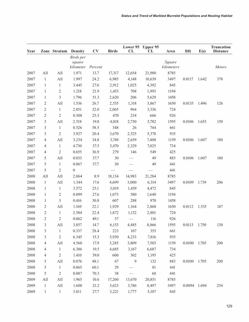
129
Status and Trend of Marbled Murrelet Populations and Nesting Habitat
Year Zone Stratum Density CV BirdsLower 95
CLUpper 95
CL Area f(0) E(s)Truncation
DistanceBirds per
square kilometer Percent
Square kilometers Meters
2007 All All 1.971 13.7 17,317 12,654 21,980 87852007 1 All 1.997 24.2 6,985 4,148 10,639 3497 0.0117 1.642 3782007 1 1 3.445 27.6 2,912 1,025 4,392 8452007 1 2 1.218 21.9 1,453 708 1,993 11942007 1 3 1.796 51.3 2,620 206 5,629 14582007 2 All 1.536 26.7 2,535 1,318 3,867 1650 0.0135 1.496 1262007 2 1 2.851 32.0 2,065 964 3,336 7242007 2 2 0.508 25.5 470 234 666 9262007 3 All 2.518 19.8 4,018 2,730 5,782 1595 0.0106 1.653 1502007 3 1 0.526 58.5 348 26 744 6612007 3 2 3.927 20.4 3,670 2,525 5,378 9352007 4 All 3.234 34.8 3,749 2,659 7,400 1159 0.0106 1.607 1802007 4 1 4.730 37.5 3,470 2,329 7,025 7342007 4 2 0.655 36.9 279 146 549 4252007 5 All 0.033 37.7 30 — 49 883 0.0106 1.607 1802007 5 1 0.067 37.7 30 — 49 4412007 5 2 0 — — — 4412008 All All 2.064 8.9 18,134 14,983 21,284 87852008 1 All 1.344 17.6 4,699 3,000 6,314 3497 0.0109 1.739 2062008 1 1 3.572 25.1 3,019 1,439 4,472 8452008 1 2 0.899 27.6 1,073 580 1,640 11942008 1 3 0.416 30.8 607 288 970 14582008 2 All 1.169 22.1 1,929 1,164 2,868 1650 0.0112 1.535 1872008 2 1 2.584 22.4 1,872 1,132 2,801 7242008 2 2 0.062 49.1 57 — 116 9262008 3 All 3.857 14.7 6,153 4,485 8,066 1595 0.0113 1.750 1302008 3 1 0.337 28.4 223 107 353 6612008 3 2 6.345 15.3 5,930 4,233 7,816 9352008 4 All 4.560 17.9 5,285 3,809 7,503 1159 0.0100 1.705 2002008 4 1 6.386 19.5 4,685 3,167 6,687 7342008 4 2 1.410 39.0 600 302 1,195 4252008 5 All 0.076 48.1 67 9 132 883 0.0100 1.705 2002008 5 1 0.065 60.1 29 — 81 4412008 5 2 0.087 70.3 38 — 68 4412009 All All 1.965 10.6 17,260 13,670 20,851 87852009 1 All 1.608 21.2 5,623 3,786 8,497 3497 0.0094 1.694 2542009 1 1 3.811 27.7 3,221 1,777 5,107 845
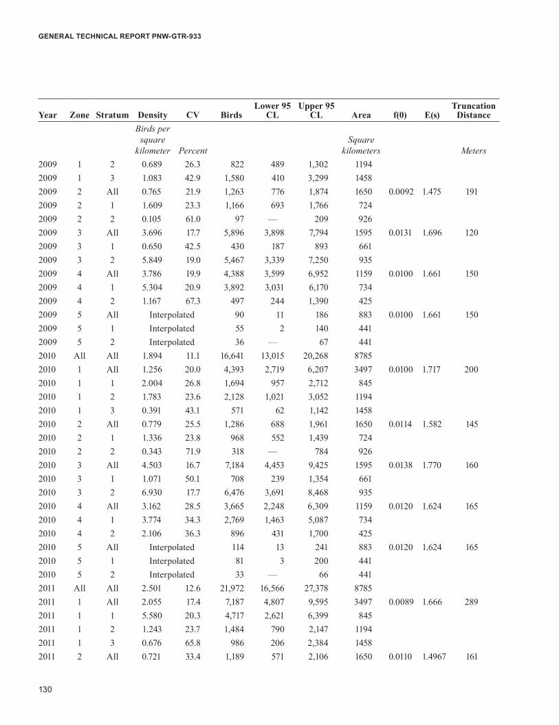
130
GENERAL TECHNICAL REPORT PNW-GTR-933
Year Zone Stratum Density CV BirdsLower 95
CLUpper 95
CL Area f(0) E(s)Truncation
DistanceBirds per
square kilometer Percent
Square kilometers Meters
2009 1 2 0.689 26.3 822 489 1,302 11942009 1 3 1.083 42.9 1,580 410 3,299 14582009 2 All 0.765 21.9 1,263 776 1,874 1650 0.0092 1.475 1912009 2 1 1.609 23.3 1,166 693 1,766 7242009 2 2 0.105 61.0 97 — 209 9262009 3 All 3.696 17.7 5,896 3,898 7,794 1595 0.0131 1.696 1202009 3 1 0.650 42.5 430 187 893 6612009 3 2 5.849 19.0 5,467 3,339 7,250 9352009 4 All 3.786 19.9 4,388 3,599 6,952 1159 0.0100 1.661 1502009 4 1 5.304 20.9 3,892 3,031 6,170 7342009 4 2 1.167 67.3 497 244 1,390 4252009 5 All Interpolated 90 11 186 883 0.0100 1.661 1502009 5 1 Interpolated 55 2 140 4412009 5 2 Interpolated 36 — 67 4412010 All All 1.894 11.1 16,641 13,015 20,268 87852010 1 All 1.256 20.0 4,393 2,719 6,207 3497 0.0100 1.717 2002010 1 1 2.004 26.8 1,694 957 2,712 8452010 1 2 1.783 23.6 2,128 1,021 3,052 11942010 1 3 0.391 43.1 571 62 1,142 14582010 2 All 0.779 25.5 1,286 688 1,961 1650 0.0114 1.582 1452010 2 1 1.336 23.8 968 552 1,439 7242010 2 2 0.343 71.9 318 — 784 9262010 3 All 4.503 16.7 7,184 4,453 9,425 1595 0.0138 1.770 1602010 3 1 1.071 50.1 708 239 1,354 6612010 3 2 6.930 17.7 6,476 3,691 8,468 9352010 4 All 3.162 28.5 3,665 2,248 6,309 1159 0.0120 1.624 1652010 4 1 3.774 34.3 2,769 1,463 5,087 7342010 4 2 2.106 36.3 896 431 1,700 4252010 5 All Interpolated 114 13 241 883 0.0120 1.624 1652010 5 1 Interpolated 81 3 200 4412010 5 2 Interpolated 33 — 66 4412011 All All 2.501 12.6 21,972 16,566 27,378 87852011 1 All 2.055 17.4 7,187 4,807 9,595 3497 0.0089 1.666 2892011 1 1 5.580 20.3 4,717 2,621 6,399 8452011 1 2 1.243 23.7 1,484 790 2,147 11942011 1 3 0.676 65.8 986 206 2,384 14582011 2 All 0.721 33.4 1,189 571 2,106 1650 0.0110 1.4967 161

131
Status and Trend of Marbled Murrelet Populations and Nesting Habitat
Year Zone Stratum Density CV BirdsLower 95
CLUpper 95
CL Area f(0) E(s)Truncation
DistanceBirds per
square kilometer Percent
Square kilometers Meters
2011 2 1 1.314 30.8 952 400 1,572 7242011 2 2 0.256 102.0 237 38 772 9262011 3 All 4.661 16.3 7,436 5,067 9,746 1595 0.0126 1.678 1202011 3 1 0.980 38.6 648 343 1,455 6612011 3 2 7.264 17.4 6,788 4,304 9,054 9352011 4 All 5.196 34.9 6,023 2,782 10,263 1159 0.0122 1.644 1452011 4 1 6.724 42.2 4,933 1,643 8,767 7342011 4 2 2.561 47.3 1,090 592 2,472 4252011 5 All 0.155 53.0 137 16 295 883 0.0122 1.644 1452011 5 1 0.243 64.8 107 5 259 4412011 5 2 0.068 78.8 30 — 66 4412012 All All 2.396 11.4 21,052 16,369 25,736 87852012 1 All 2.414 20.7 8,442 5,090 12,006 3497 0.0109 1.847 1642012 1 1 7.166 24.4 6,056 3,289 8,823 8452012 1 2 1.507 30.4 1,799 812 2,892 11942012 1 3 0.402 48.1 587 168 1,227 14582012 2 All 0.719 33.5 1,186 564 2,360 1650 0.0132 1.485 1062012 2 1 1.178 29.2 853 325 1,289 7242012 2 2 0.360 89.9 333 — 1,459 9262012 3 All 3.986 15.5 6,359 4,136 8,058 1595 0.0112 1.765 1862012 3 1 0.895 34.9 591 227 1,042 6612012 3 2 6.172 15.9 5,768 3,775 7,330 9352012 4 All 4.279 24.9 4,960 3,414 8,011 1159 0.0107 1.652 1402012 4 1 6.050 27.6 4,439 2,916 7,497 7342012 4 2 1.225 39.6 521 166 940 4252012 5 All Interpolated 104 10 206 883 0.0107 1.652 1402012 5 1 Interpolated 89 5 189 4412012 5 2 Interpolated 15 — 33 4412013 All All 2.238 11.1 19,662 15,398 23,927 87852013 1 All 1.257 27.9 4,395 2,298 6,954 3497 0.0109 1.695 1372013 1 1 2.379 31.4 2,010 861 3,253 8452013 1 2 0.657 20.1 784 508 1,124 11942013 1 3 1.097 64.4 1,600 381 3,717 14582013 2 All 0.770 18.5 1,271 950 1,858 1650 0.0117 1.569 1322013 2 1 1.605 19.0 1,163 854 1,722 7242013 2 2 0.117 59.3 108 — 274 9262013 3 All 4.939 16.3 7,880 5,450 10,361 1595 0.0112 1.637 160

132
GENERAL TECHNICAL REPORT PNW-GTR-933
Year Zone Stratum Density CV BirdsLower 95
CLUpper 95
CL Area f(0) E(s)Truncation
DistanceBirds per
square kilometer Percent
Square kilometers Meters
2013 3 1 0.991 43.8 655 151 1,226 6612013 3 2 7.731 17.8 7,225 4,707 9,667 9352013 4 All 5.216 20.5 6,046 4,531 9,282 1159 0.0128 1.607 1462013 4 1 7.384 21.8 5,418 3,939 8,516 7342013 4 2 1.477 36.7 629 279 1,184 4252013 5 All 0.080 45.4 71 5 118 883 0.0128 1.607 1462013 5 1 0.160 45.4 71 5 118 4412013 5 2 0 — — — 441CV = coefficient of variation; CL = confidence limit


Pacific Northwest Research Station
Website http://www.fs.fed.us/pnw/Telephone (503) 808–2592Publication requests (503) 808–2138FAX (503) 808–2130E-mail [email protected] address Publications Distribution Pacific Northwest Research Station P.O. Box 3890 Portland, OR 97208–3890
U.S. Department of Agriculture Pacific Northwest Research Station 1220 SW 3rd Ave. P.O. Box 3890 Portland, OR 97208–3890
Official Business Penalty for Private Use, $300