Nonparametric models of financial leverage decisions

Joao A. Bastosa∗ Joaquim J. S. Ramalhob†

aCEMAPRE, School of Economics and Management (ISEG),

Technical University of Lisbon, Portugal

bDepartment of Economics and CEFAGE,

University of Evora, Portugal

Abstract

This paper investigates the properties of nonparametric decision tree models in the anal-

ysis of financial leverage decisions. This approach presents two appealing features: the

relationship between leverage ratios and the explanatory variables is not predetermined

but is derived according to information provided by the data, and the models respect the

bounded and fractional nature of leverage ratios. The analysis shows that tree models sug-

gest relationships between explanatory variables and the relative amount of issued debt that

parametric models fail to capture. Furthermore, the significant relationships found by tree

models are in most cases in accordance with the effects predicted by the pecking-order the-

ory. The results also show that two-part tree models can accommodate better the distinct

effects of explanatory variables on the decision to issue debt and on the amount of debt

issued by firms that do resort to debt.

JEL Classification: C14, C35, G32.

Keywords: Capital structure; Fractional regression; Decision tree; Two-part model.

This version: April 2011

∗E-mail address: jbastos@iseg.utl.pt†E-mail address: jsr@uevora.pt

1

1 Introduction

One important issue in the corporate finance literature is the analysis of the factors that affect

firms’ capital structure decisions. To measure the financial leverage of firms, it is typically

used some ratio of debt to capital assets, which, by definition, is observed only on the unit

interval [0,1]. Given the bounded and fractional nature of the variable of interest, it has been

recently advocated by several authors (e.g., Cook et al., 2008; Ramalho and Silva, 2009) that the

regression analysis of leverage ratios should be carried out using Papke and Wooldridge (1996)

fractional regression model, which was specifically developed for modeling proportions. Because

many firms usually have null leverage ratios, Ramalho and Silva (2009) suggested also the use

of two-part models to explain financial leverage decisions. In such models, first, a binary choice

model is used to explain the probability of a firm raising debt; then, a fractional regression

model is employed to explain the relative amount of debt issued by firms that do use debt.

Conceptually, it is clear that fractional regression models (or their two-part variants) are

more suitable to model leverage ratios than the linear or tobit models that traditionally were

used in capital structure empirical studies. For example, an obvious problem with the appli-

cation of linear or (censored-at-zero) tobit models in this context is that the predicted values

of leverage ratios are not constrained to the unit interval. However, a crucial assumption in

the use of fractional (or binary) regression models is the correct specification of the conditional

expectation of the response variable. As found by Ramalho et al. (2011), using an incorrect

functional form for that expectation may lead to distorted results in the assessment of the sta-

tistical relevance of explanatory variables and in the estimation of partial affects. To deal with

this issue, Ramalho et al. (2011) proposed various specification tests for assessing the condi-

tional mean assumption underlying fractional regression models, which are also valid for testing

the binary specifications used in two-part models. Nevertheless, because in some cases it may

be complicated to find a suitable parametric model, it would be interesting the development of

econometric models that do not require a priori the choice of a functional form for the condi-

tional mean of the response variable but take into account the fractional or binary nature of

the dependent variable. This may be accomplished with nonparametric models, in which the

relationship between the variable of interest and explanatory variables is not predetermined by

the researcher but is derived from information provided by the data.

This paper investigates the ability of nonparametric decision trees (Breiman at al., 1984;

Quinlan, 1986) to model both the decision to issue debt and the decision on the relative amount

of debt to be issued by those firms which resort to debt. Decision trees are one of the sim-

plest techniques of pattern recognition. They possess the valuable capability of tackling both

classification and regression problems. Therefore, decision trees can simultaneously model both

the firm’s decision to issue debt or not (the classification problem) and the amount of debt to

be issued (the regression problem). Decision trees derive their predictive power by recursively

partitioning the original data set into smaller mutually exclusive subsets using a greedy search

algorithm. Starting from the root node, all observations are routed down the tree according

to the values of the attributes tested in successive nodes and terminate their path in some

2

terminal node. In classification problems, an observation is classified according to the most

prevalent class in the terminal node where it terminates its path. In regression problems, the

value predicted for the response variable of an observation is given by the average value of the

response variable for all observations contained in its terminal node. This feature is crucial:

because predicted values are averages of actual values, when the response variable is bounded

to the unit interval [0,1], predicted values will inevitably be also bounded between 0 and 1, as

in standard fractional regression models.

In the finance literature, decision trees are not an unfamiliar tool for modeling proportions,

especially when the aim is forecasting. For instance, Bastos (2010) showed that regression trees

are a competitive technique with respect to parametric fractional regression models in predicting

the fraction of a defaulted loan that is recovered by a bank in a bankruptcy resolution process.

This paper shows that decision tree models may be also a competitive technique when the main

interest is studying the statistical relevance of a set of explanatory variables, as is typical in

capital structure empirical studies. In fact, in addition to not requiring the specification of a

functional form for the conditional mean of the response variable, decision tree models have

another important advantage over parametric models: each explanatory variable is allowed to

affect in different ways firms assigned to different terminal nodes. This implies, for example,

that: (i) some variables may be relevant to explain the financial leverage decisions of some firms

but not of others; and (ii) some variables may have a positive impact on the response variable for

some firms and negative for others. In contrast, in the parametric framework similar results are

only possible, and only to some extent, if the empirical researcher is able to include appropriate

dummy variables and interaction variables in the regression equation. To illustrate and evaluate

the application of decision tree models in this context, this paper uses the data set of Ramalho

and Silva (2009) and compares their performance with that of the two-part logistic regression

model employed by those authors.

This paper is organized as follows. Section 2 briefly reviews some capital structure theories

and parametric two-part fractional regression models. Section 3 discusses the decision tree

models. Section 4 is dedicated to the empirical application. Finally, Section 5 presents some

concluding remarks.

2 Framework

Since the main purpose of this study is to understand how decision tree models may be used

to explain both the probability of a firm using debt and the relative amount of debt that is

issued, this paper focus on the use of two-part models in the analysis of the determinants of

financial leverage decisions. This section first reviews some theoretical arguments that justify

the employment of those models in capital structure empirical studies. Then, it briefly describes

the main characteristics of the parametric two-part fractional regression models that will be used

as benchmark in the evaluation of the performance of the two-part decision tree models.

3

2.1 Capital structure theories: one-part versus two-part models

Up to date, most capital structure empirical studies have used ‘one-part’ models to explain

leverage ratios, which follows directly from the fact that most capital structure theories provide

a single explanation for all possible values of leverage ratios, including the value zero. This

is the case, for example, of the most popular explanations of capital structure decisions, the

trade-off and the pecking-order theories. The trade-off theory claims that firms set a target

level for their debt-equity ratio that balances the tax advantages of additional debt against the

costs of possible financial distress and bankruptcy. From this value optimization problem, it

may result for leverage ratios any value in the unit interval, including zero. The pecking-order

theory, on the other hand, argues that, due to information asymmetries between firms’ managers

and potential outside financiers, firms tend to adopt a perfect hierarchical order of financing:

first, they use internal funds (retained earnings); in case external financing is needed, they issue

low-risk debt; only as a last resort, when the firm exhausts its ability to issue safe debt, are new

shares issued. Hence, the firm leverage at each moment merely reflects its external financing

requirements, which may be null or any positive amount. For details on both theories, see inter

alia the recent survey by Frank and Goyal (2008).

In contrast to these traditional approaches, Kurshev and Strebulaev (2007) and Strebulaev

and Yang (2007) have recently argued that zero-leverage behavior is a persistent phenomenon

and that standard capital structure theories are unable to provide a reasonable explanation

for it. In particular, they found that while larger firms are more likely to have some debt,

conditional on having some debt, larger firms are less levered, that is, firm size seems to affect

in an inverse way the participation and amount debt decisions. According to these authors, the

opposite effects of firm size on leverage may be explained by the presence of fixed costs of external

financing, and the consequent infrequent refinancing of firms, since smaller firms are much more

affected in relative terms than larger firms. Thus: (i) small firms choose higher leverage at

the moment of refinancing to compensate for less frequent rebalancing, which explains why,

conditional on having debt, they are more levered than large firms; (ii) as they wait longer

times between refinancings, small firms, on average, have lower levels of leverage; and (iii) in

each moment, there is a mass of firms opting for no leverage, since small firms may find it

optimal to postpone their debt issuances until their fortunes improve substantially relative to

the costs of issuance. Clearly, in this framework, a two-part fractional regression model may be

the best option for modeling leverage ratios, since the variable size (and others) is allowed to

influence each decision in a different fashion.

2.2 Parametric two-part fractional regression model

Let y be the variable of interest (i.e., the leverage ratio), with 0 ≤ y < 1, x be the vector of

explanatory variables and z be a binary indicator that takes the values of unity and zero for

4

firms that use debt and firms that have null leverage ratios, respectively. Then,

z =

{1 for 0 < y < 1

0 for y = 0(1)

The parametric two-part model proposed for explaining firms’ capital structure decisions has

two components: one binary and the other fractional. The binary component (the first part)

of the two-part model comprises a standard binary choice model to explain the probability of a

firm choosing to use debt or not:

Pr (z = 1|x) = F (xβ1P ) , (2)

where β1P is a vector of coefficients and F (·) is a cumulative distribution function (e.g. that

defining logit or probit models). The fractional component (the second part) of the model

contemplates only the sub-sample of firms that do use debt and estimates the relative amount

of debt issued by them:

E (y|x, y ∈ ]0, 1[) = M (xβ2P ) , (3)

where M (·) is some nonlinear function satisfying 0 < M (·) < 1, and β2P is another vector of

coefficients. Clearly, one may consider for M (·) the same specifications as those for F (·) in the

binary component of the model.

The overall conditional mean of y can be written as

E (y|x) = Pr (z = 1|x) · E (y|x, y ∈ ]0, 1[)

= F (xβ1P ) ·M (xβ2P ) . (4)

As β1P and β2P are not required to be the same, the two-part model allows the explanatory

variables to influence in independent ways the firm’s choice of using or not using debt and the

firm’s choice of debt proportion. For simplicity, it is assumed that the same covariates appear

in both components of the model, but this assumption can be relaxed and, in fact, should be if

there are obvious exclusion restrictions. See Ramalho et al. (2011) for details on the estimation

of two-part models for fractional data.

The crucial assumption for estimating both β1P and β2P consistently is the correct formal-

ization of E (y|x), which, in turn, requires that both Pr (z = 1|x) and E (y|x, y ∈ ]0, 1[) are

properly specified. In this paper, the results produced by decision tree models are compared

with those obtained in Ramalho and Silva (2009), where a logistic specification was adopted for

both components of the two-part model:

E (y|x) = exβ1P

1 + exβ1P

exβ2P

1 + exβ2P. (5)

5

3 Decision tree models

As mentioned in the introductory section, decision trees are nonparametric and nonlinear pre-

dictive models in which the original data set is recursively partitioned into smaller mutually

exclusive subsets using a greedy search algorithm. Tree models are represented by a sequence of

logical if-then-else tests on the attributes of the observations. Decision trees can be employed

in both classification and regression problems and, therefore, can model both the firm’s decision

to issue debt or not and the amount of debt to be issued.

3.1 Classification trees

Suppose one has a set of observations (i.e., firms) described by a vector of attributes x, and that

these observations belong to each of two classes (i.e., firms that issue debt and firms that don’t).

The goal of a classification tree is to separate as well as possible the observations that belong to

one class from those that belong to the other through a sequence of binary splits of the data.1

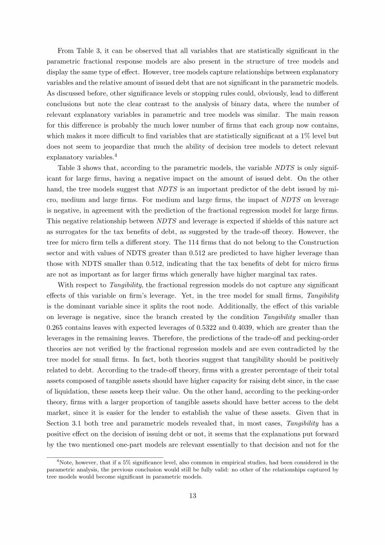
The algorithm begins with a root node containing all observations. Then, the algorithm loops

over all possible binary splits in order to find the attribute xi, i = 1, ..., N , and corresponding

cut-off value ci which gives the best separation into one side having mostly observations from

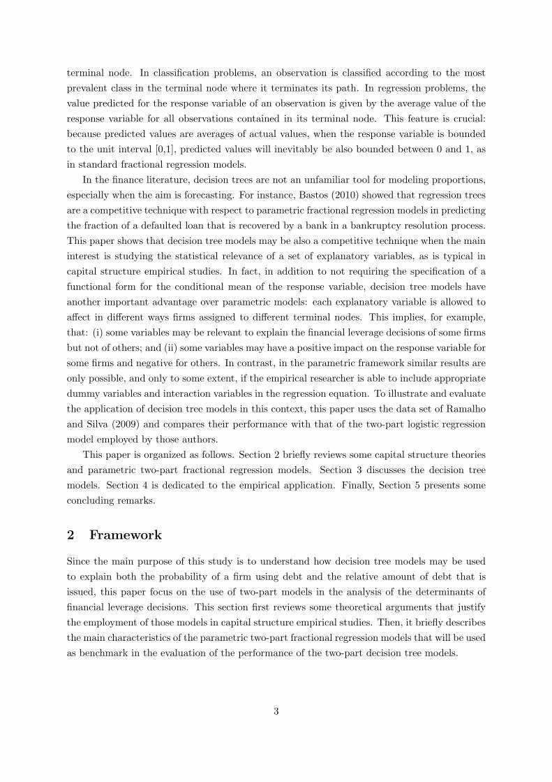
one class and the other mostly observations from the other. For example, Figure 1 represents

a hypothetical classification tree in which the best separation is achieved when the data in the

root node is split between observations having attribute xi ≤ ci and those having xi > ci. This

procedure is then repeated for the new daughter nodes until no further improvement in class

separation is achieved or a stopping criterion is satisfied. Unsplit terminal nodes are referred

by the figurative term of leaves, and are depicted by rectangles in the schemes representing

decision trees.

Figure 1 about here

How are the optimal attribute and cut-off value defined? Denote by p the number of obser-

vations of one class and by n the number observations of the other class contained in a given

node. The entropy E(p, q) of that node is defined as

E(p, q) = − p

p+ nlog2

(p

p+ n

)− n

p+ nlog2

(n

p+ n

). (6)

Now, suppose that a given binary split of the data leaves p1 and n1 observations of each class in

one daughter node, and p2 and n2 observations of each class in the other. The optimal splitting

attribute and corresponding cut-off value are those that maximize the information gain

gain = E(p, q)− p1 + n1

p+ nE(p1, q1)−

p2 + n2

p+ nE(p2, q2). (7)

1Classification trees are not restricted to binary splits. That is, at each step the data can be divided in threeor more subsets. For computational convenience the models developed in this study are constructed using onlybinary divisions.

6

Positive information gains result in reductions of entropy. Since the entropy characterizes the

diversity of the population in a node, maximizing the information gain results in daughter nodes

that are more homogeneous than the parent nodes.

Starting from the root node, all observations are routed down the tree according to the

values of the attributes tested in successive nodes and, inevitably, terminate their path in a

leaf. In the end, observations are classified according to the most prevalent class in the leaf

where they terminated their path. The growth process usually results in trees that are quite

large and not easily interpretable. Furthermore, these trees will overfit the data, giving good

classification accuracies on the data employed in the growth process but poor accuracies on new

data. Improved accuracies on unobserved data can be obtained by “pruning” the tree after the

basic growth process. The pruning procedure examines each node of the tree, starting at the

bottom. An estimate of the expected classification accuracy that will be experienced at each

node for unobserved data is evaluated. If the accuracy of a subtree is smaller than the accuracy

of the parent node, then the parent node is pruned to a leaf. This process is repeated until

pruning no longer improves the accuracy.2

3.2 Regression trees

Regression trees are conceptually similar to classification trees, but now the target is not a

discrete set of classes but a numeric variable (i.e., leverage ratio). In the construction of a

regression tree, one searches over all possible binary splits of all available attributes for the

one which will minimize the intra-subset variation of the target variable in the newly created

daughter nodes. That is, in each daughter node the target variable will be more homogeneous

than in the parent node. Again, the procedure is repeated recursively for new daughter nodes

until no further reduction in the variation of the target variable is achievable. The decrease in

the variance of the target variable is measured by the standard deviation reduction,

SDR = s(T )− m(T1)

m(T )s(T1)−

m(T2)

m(T )s(T2), (8)

where T is the set of observations in the parent node, and T1 and T2 are the set of observations in

the daughter nodes that result from splitting the parent node according to the optimal attribute

and cut-off value. The operatorsm(·) and s(·) represent the sample mean and standard deviation

of the target variable in the set. The predictions of the model are given by the average value

of the target variable for the set of observations in each leaf. Note that predicted values for

target variables bounded to the unit interval will inevitably be bounded to the unit interval.

Therefore, regression trees are particularly appropriate for modeling leverage ratios.

In order to avoid overfitting the data and reduce the error of the model on unobserved data,

regression trees are also pruned after the growth process. The pruning procedure is analogous

to that of classification trees. First, an estimate of the expected variance of the target variable

2A comprehensive description of the tree growth and pruning algorithms is beyond the scope of this paper.The reader is referred to Witten and Frank (2005) for technical details of the algorithms employed here.

7

that will be experienced at each node for unobserved data is evaluated. Then, if the variance of

a subtree is greater than the variance of the parent node, the parent node is pruned to a leaf.

This process is repeated until pruning no longer improves the error.

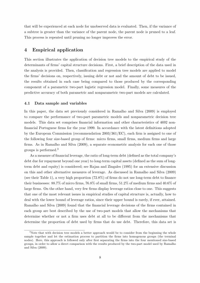
4 Empirical application

This section illustrates the application of decision tree models to the empirical study of the

determinants of firms’ capital structure decisions. First, a brief description of the data used in

the analysis is provided. Then, classification and regression tree models are applied to model

the firms’ decisions on, respectively, issuing debt or not and the amount of debt to be issued,

the results obtained in each case being compared to those produced by the corresponding

component of a parametric two-part logistic regression model. Finally, some measures of the

predictive accuracy of both parametric and nonparametric two-part models are calculated.

4.1 Data sample and variables

In this paper, the data set previously considered in Ramalho and Silva (2009) is employed

to compare the performance of two-part parametric models and nonparametric decision tree

models. This data set comprises financial information and other characteristics of 4692 non-

financial Portuguese firms for the year 1999. In accordance with the latest definitions adopted

by the European Commission (recommendation 2003/361/EC), each firm is assigned to one of

the following four size-based group of firms: micro firms, small firms, medium firms and large

firms. As in Ramalho and Silva (2009), a separate econometric analysis for each one of those

groups is performed.3

As a measure of financial leverage, the ratio of long-term debt (defined as the total company’s

debt due for repayment beyond one year) to long-term capital assets (defined as the sum of long-

term debt and equity) is considered; see Rajan and Zingales (1995) for an extensive discussion

on this and other alternative measures of leverage. As discussed in Ramalho and Silva (2009)

(see their Table 1), a very high proportion (72.8%) of firms do not use long-term debt to finance

their businesses: 88.7% of micro firms, 76.8% of small firms, 51.2% of medium firms and 40.6% of

large firms. On the other hand, very few firms display leverage ratios close to one. This suggests

that one of the most relevant issues in empirical studies of capital structure is, actually, how to

deal with the lower bound of leverage ratios, since their upper bound is rarely, if ever, attained.

Ramalho and Silva (2009) found that the financial leverage decisions of the firms contained in

each group are best described by the use of two-part models that allow the mechanisms that

determine whether or not a firm uses debt at all to be different from the mechanisms that

determine the proportion of debt used by firms that do use debt. Therefore, this data set is

3Note that with decision tree models a better approach would be to consider from the beginning the wholesample together and let the estimation process to partition the firms into homogenous groups (the terminalnodes). Here, this approach is followed only after first separating the firms into the four mentioned size-basedgroups, in order to allow a direct comparison with the results produced by the two-part model used by Ramalhoand Silva (2009).

8

particularly appropriate for the purposes of this paper, since, in order to exemplify the ability

of tree models in both classification and regression problems, the two sequential decisions made

by firms have to be modeled separately.

In all alternative regression models estimated next, the same explanatory variables as those

employed by Ramalho and Silva (2009) are contemplated: Non-debt tax shields (NDTS ), mea-

sured by the ratio between depreciation and earnings before interest, taxes and depreciation;

Tangibility, the proportion of tangible assets and inventories in total assets; Size, the natural

logarithm of sales; Profitability, the ratio between earnings before interest and taxes and total

assets; Growth, the yearly percentage change in total assets; Age, the number of years since

the foundation of the firm; Liquidity, the sum of cash and marketable securities, divided by

current assets; and four activity sector dummies: i) Manufacturing ; ii) Construction; iii) Trade

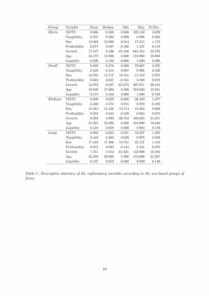
(wholesale and retail); and iv) Transport and Communication. Table 1 reports the descriptive

statistics of the explanatory variables according to the four size-based groups of firms considered

in this analysis.

Table 1 about here

The variables in Table 1 are some of the most common explanatory variables used in capital

structure empirical studies, both in one-part and two-part models. According to one-part

models, some of those variables are expected to have a positive impact on leverage ratios (e.g.

Profitability and Liquidity, in the case of the trade-off theory; Growth, in the case of the pecking-

order theory; and Tangibility and Size, in both cases), while other are expected to have a negative

effect (e.g. NDTS and Growth, in the former theory; and Profitability, Age and Liquidity, in

the latter); see inter alia Frank and Goyal (2008) for an explanation of these effects. Regarding

two-part models, each factor is allowed to influence in distinct manners each decision, the focus

so far being on the distinct effects of Size on the decisions to use debt or not, and on the amount

of debt issued, as described in Section 2.1.

4.2 Modeling the decision to issue debt

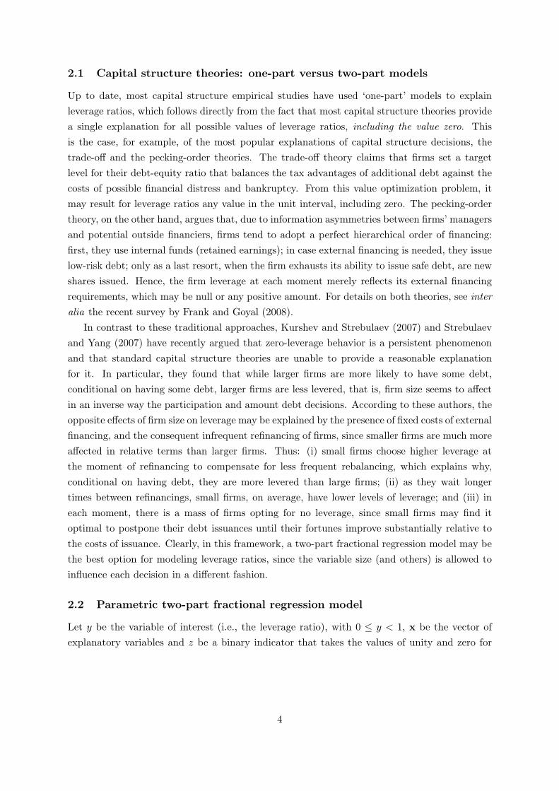
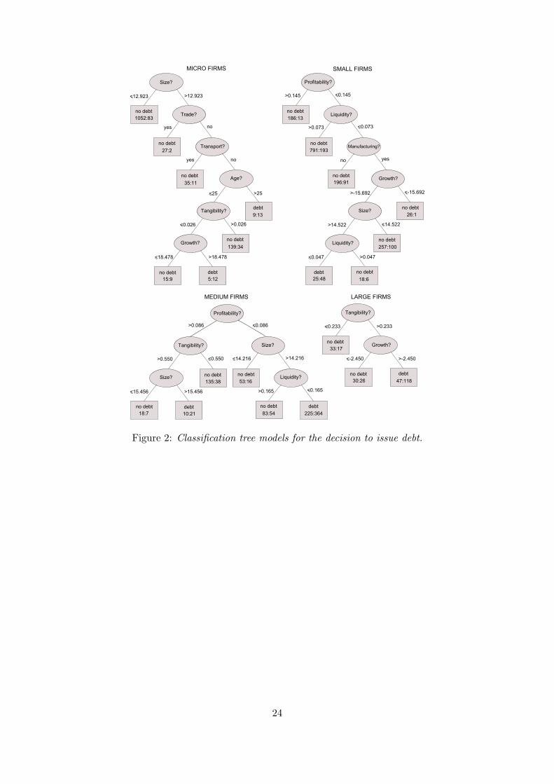
In this section, the models for the decision to issue debt are analyzed. In Figure 2, one can

find the classification tree models for the four sized-based groups of firms. The labels n : p on

the bottom of the leaves represent the numbers n and p of unleveraged and leveraged firms,

respectively, that terminated their paths in the leaves. As mentioned in Section 3.1, a leaf is

tagged according to the most prevalent class in it: if n > p the label “no debt” is given to the

leaf, otherwise the label “debt” is given.

Figure 2 about here

In Figure 2, it can be observed that the tree structure for micro and small firms is more

complex than that for medium and, mainly, large firms. This is possibly related to the smaller

number of larger firms in the sample but it may be also interpreted as a natural consequence of

the more rigorous analysis from potential lenders to which smaller firms are typically subject.

9

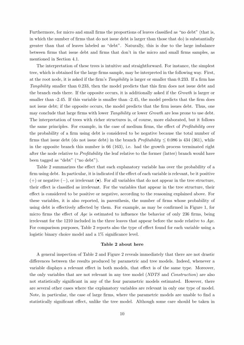
Furthermore, for micro and small firms the proportions of leaves classified as “no debt” (that is,

in which the number of firms that do not issue debt is larger than those that do) is substantially

greater than that of leaves labeled as “debt”. Naturally, this is due to the large imbalance

between firms that issue debt and firms that don’t in the micro and small firms samples, as

mentioned in Section 4.1.

The interpretation of these trees is intuitive and straightforward. For instance, the simplest

tree, which is obtained for the large firms sample, may be interpreted in the following way. First,

at the root node, it is asked if the firm’s Tangibility is larger or smaller than 0.233. If a firm has

Tangibility smaller than 0.233, then the model predicts that this firm does not issue debt and

the branch ends there. If the opposite occurs, it is additionally asked if the Growth is larger or

smaller than -2.45. If this variable is smaller than -2.45, the model predicts that the firm does

not issue debt; if the opposite occurs, the model predicts that the firm issues debt. Thus, one

may conclude that large firms with lower Tangibility or lower Growth are less prone to use debt.

The interpretation of trees with richer structures is, of course, more elaborated, but it follows

the same principles. For example, in the case of medium firms, the effect of Profitability over

the probability of a firm using debt is considered to be negative because the total number of

firms that issue debt (do not issue debt) in the branch Profitability ≤ 0.086 is 434 (361), while

in the opposite branch this number is 66 (163), i.e. had the growth process terminated right

after the node relative to Profitability the leaf relative to the former (latter) branch would have

been tagged as “debt” (“no debt”).

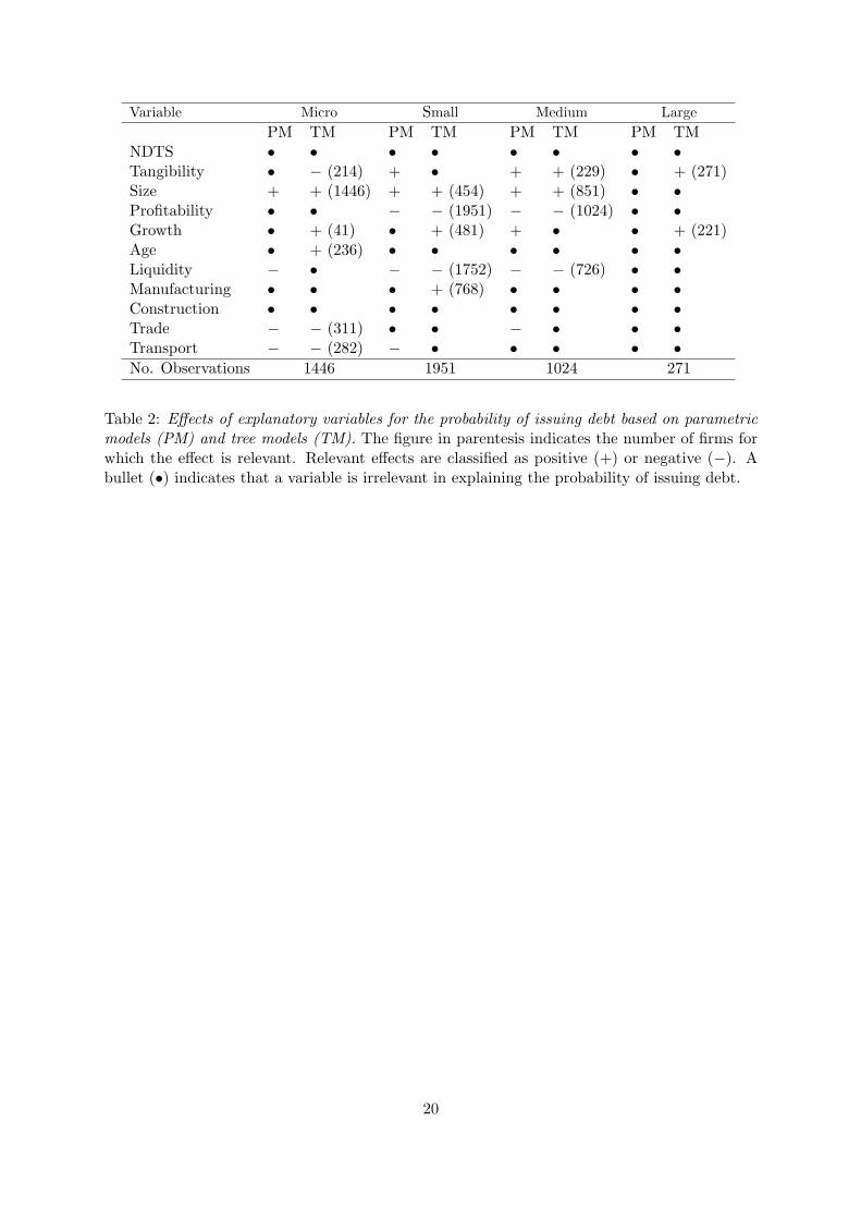
Table 2 summarizes the effect that each explanatory variable has over the probability of a

firm using debt. In particular, it is indicated if the effect of each variable is relevant, be it positive

(+) or negative (−), or irrelevant (•). For all variables that do not appear in the tree structure,

their effect is classified as irrelevant. For the variables that appear in the tree structure, their

effect is considered to be positive or negative, according to the reasoning explained above. For

these variables, it is also reported, in parenthesis, the number of firms whose probability of

using debt is effectively affected by them. For example, as may be confirmed in Figure 1, for

micro firms the effect of Age is estimated to influence the behavior of only 236 firms, being

irrelevant for the 1210 included in the three leaves that appear before the node relative to Age.

For comparison purposes, Table 2 reports also the type of effect found for each variable using a

logistic binary choice model and a 1% significance level.

Table 2 about here

A general inspection of Table 2 and Figure 2 reveals immediately that there are not drastic

differences between the results produced by parametric and tree models. Indeed, whenever a

variable displays a relevant effect in both models, that effect is of the same type. Moreover,

the only variables that are not relevant in any tree model (NDTS and Construction) are also

not statistically significant in any of the four parametric models estimated. However, there

are several other cases where the explanatory variables are relevant in only one type of model.

Note, in particular, the case of large firms, where the parametric models are unable to find a

statistically significant effect, unlike the tree model. Although some care should be taken in

10

the interpretation of these differences, since the criteria (significance level or stopping criterion)

to decide which variables are relevant are not directly comparable across models, note that,

overall, for the four size-based groups of firms, tree and parametric models give rise to a similar

number of relevant explanatory variables (17 and 15, respectively) but only in ten cases there

are coincidence of findings.

As predicted by the trade-off and pecking-order theories, the parametric binary model indi-

cates that Tangibility has a significant positive effect on the resort to debt by small and medium

firms. This result is corroborated by the tree model for medium and large firms. Interestingly,

Tangibility also participates in the tree for micro firms but, in this case, it has a negative im-

pact on the decision to issue debt, since the condition Tangibility > 0.026 leads to a “no debt”

leaf. However, note that this negative effect applies only to 14.8% of the micro firms sample,

namely those that are relatively young (Age ≤ 25), are not in the Trade or Transport sectors

and have Size greater than 12.923. This illustrates clearly one of the main advantages of using

decision tree models: the possibility of detecting automatically effects which are relevant only

for a specific group of firms. In this particular case, the negative effect of Tangibility may be

accounted for the fact that the most important form of collateral for many micro firms are

personal guarantees that allow the bank to collect the debt against personal assets pledged by

the owner, which implies that Tangibility is likely to be capturing the effects of other factors.

With regard to Size, both parametric and tree models suggest a positive relationship between

this variable and the use of debt for micro, small and medium firms, as predicted by all the three

capital structure theories mentioned in Section 2.1. The fact that the positive effect of Size is

particularly relevant for smaller firms is reinforced by the analysis of the tree for micro firms:

since it splits the root node of the tree, Size is the most relevant variable for explaining the

probability of a firm using debt, influencing the behavior of all the 1446 micro firms contained in

the sample. Actually, revealing explicitly in any analysis which is the most relevant explanatory

variable is clearly another nice feature of decision tree models.

With respect to Profitability and Liquidity, the parametric models indicate that these vari-

ables are negatively related to the decision to use debt for micro (only Liquidity), small and

medium firms. The trees for small and medium firms substantiate this observation and, in

addition, show that: (i) Profitability is the most relevant variable for explaining the decision

of these firms to resort or not to debt; and (ii) Liquidity is also a very important factor, in-

fluencing the decision of 89.8% of small firms and 70.9% of medium firms. Thus, for small

and medium firms both estimation techniques support strongly the pecking-order theory and

provide evidence against the trade-off theory.

The parametric binary models indicate that Growth has a significant positive impact on the

decision to use debt for medium firms, while the classification trees for micro, small and large

firms suggest that smaller values of Growth lead some firms to the decision of not resorting to

debt. Although the results produced by each technique are not in accordance with each other,

and clearly Growth is not the most relevant variable for any group, overall it seems that both

models partially validate the pecking-order theory and provide evidence against the trade-off

11

theory.

The nonparametric method also reveals that the age of micro firms has a positive impact on

the decision to issue debt, provided that they are not that “micro” (Size > 12.923 - the mean

of Size in the micro firms group is 12.063, see Table 1) and do not operate in the Trade or

Transport sectors. For these specific firms, it may seem that the pecking-order theory does not

fully apply, since in that framework it is commonly argued that older firms tend to accumulate

retained earnings and, thus, require less external finance. However, it turns out that it is possible

to explain the positive effect that Age has on the probability of a micro firm issuing debt using

information asymmetry arguments of the type also usually considered by the pecking-order

theory. Indeed, most micro firms, particularly the younger ones, are characterized by severe

informational opacity. Thus, older micro firms of a reasonable size may be more prone to use

debt because they tend to display less opaqueness on the quality of their management and the

value of their assets, implicating that lenders trust them more.

Overall, the results obtained in this section support the pecking-order theory in detriment

of the trade-off theory. The effect found for the variable Size is also in accordance with that

predicted by the two-part theory. In general, the conclusions achieved by Ramalho and Silva

(2009) using parametric models were corroborated and reinforced by the nonparametric decision

tree models, namely the very special relevancy that the variables Size for micro firms and

Profitability and Liquidity for small and medium firms have on the decision to use debt or not.

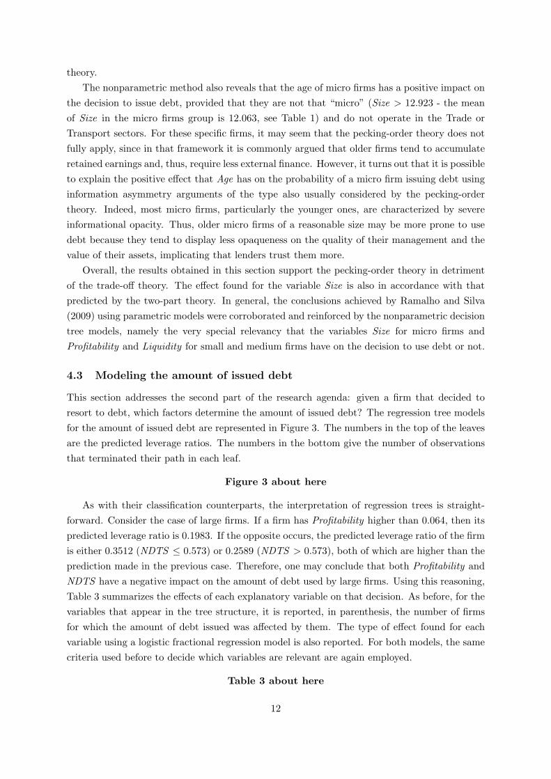
4.3 Modeling the amount of issued debt

This section addresses the second part of the research agenda: given a firm that decided to

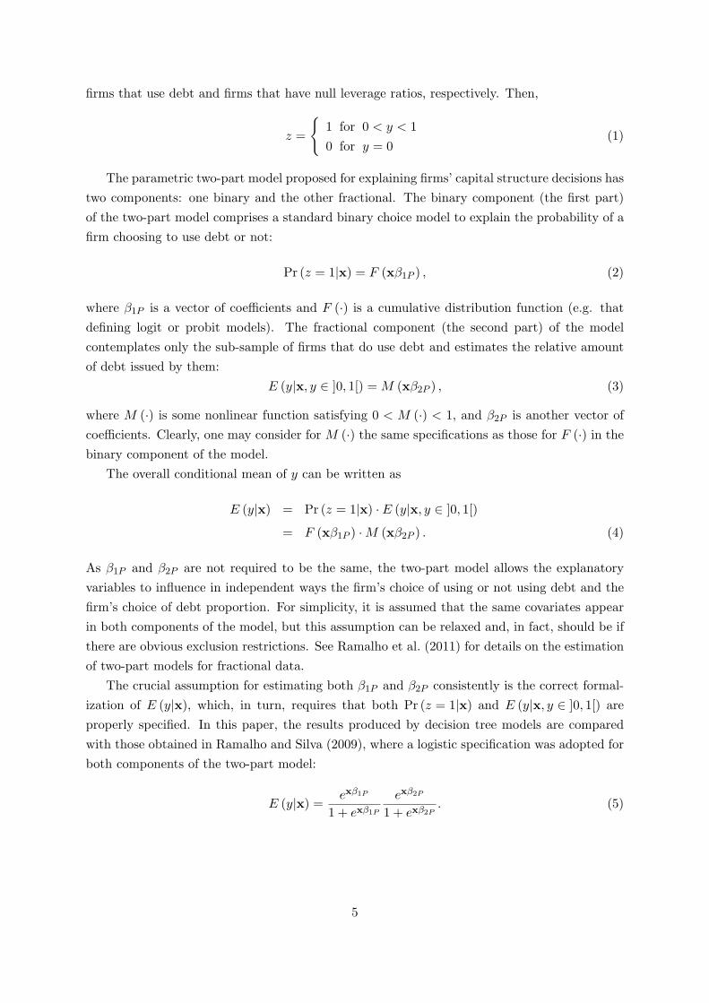
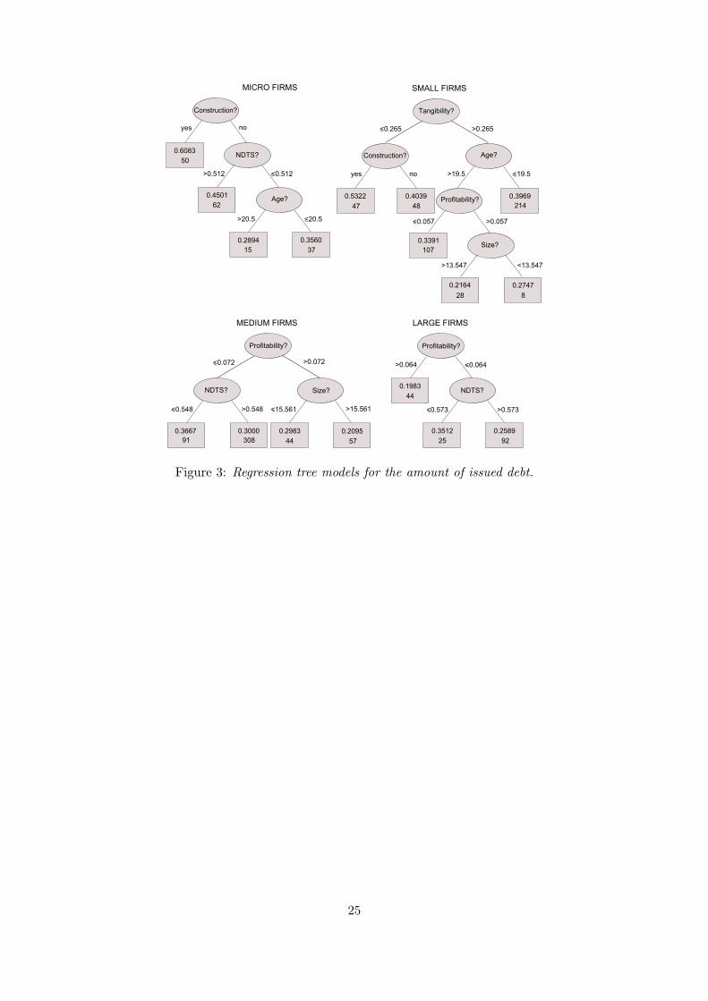
resort to debt, which factors determine the amount of issued debt? The regression tree models

for the amount of issued debt are represented in Figure 3. The numbers in the top of the leaves

are the predicted leverage ratios. The numbers in the bottom give the number of observations

that terminated their path in each leaf.

Figure 3 about here

As with their classification counterparts, the interpretation of regression trees is straight-

forward. Consider the case of large firms. If a firm has Profitability higher than 0.064, then its

predicted leverage ratio is 0.1983. If the opposite occurs, the predicted leverage ratio of the firm

is either 0.3512 (NDTS ≤ 0.573) or 0.2589 (NDTS > 0.573), both of which are higher than the

prediction made in the previous case. Therefore, one may conclude that both Profitability and

NDTS have a negative impact on the amount of debt used by large firms. Using this reasoning,

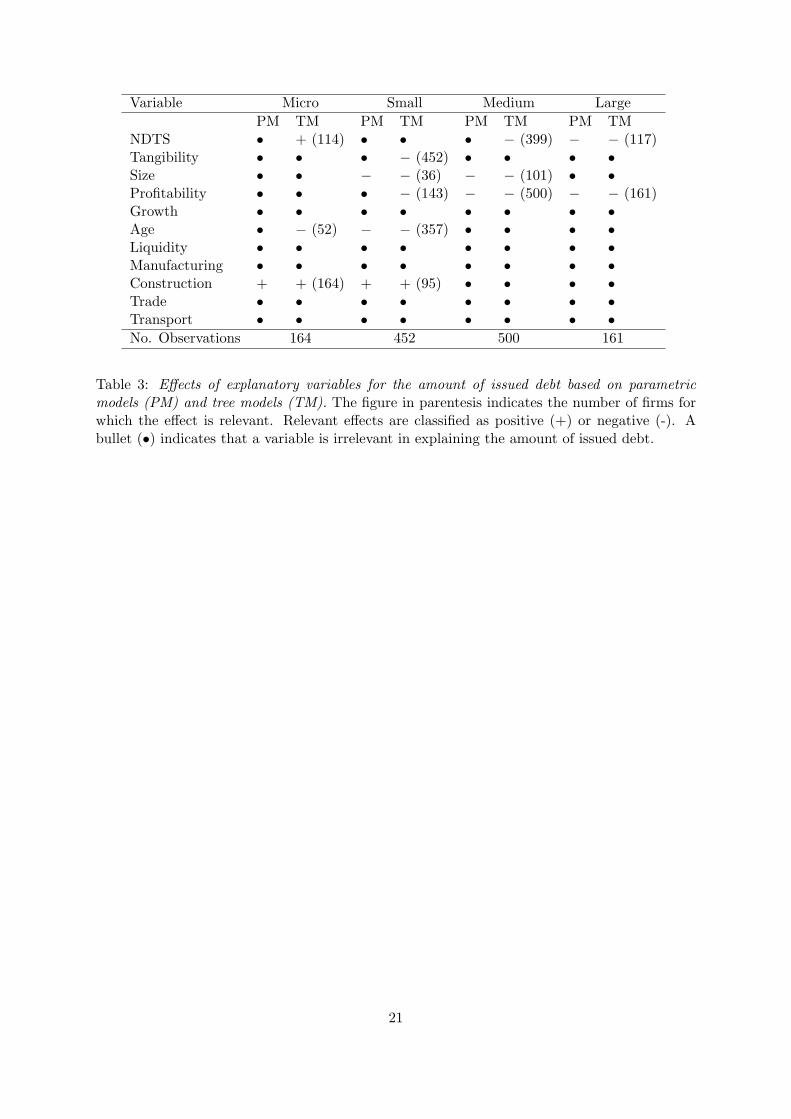
Table 3 summarizes the effects of each explanatory variable on that decision. As before, for the

variables that appear in the tree structure, it is reported, in parenthesis, the number of firms

for which the amount of debt issued was affected by them. The type of effect found for each

variable using a logistic fractional regression model is also reported. For both models, the same

criteria used before to decide which variables are relevant are again employed.

Table 3 about here

12

From Table 3, it can be observed that all variables that are statistically significant in the

parametric fractional response models are also present in the structure of tree models and

display the same type of effect. However, tree models capture relationships between explanatory

variables and the relative amount of issued debt that are not significant in the parametric models.

As discussed before, other significance levels or stopping rules could, obviously, lead to different

conclusions but note the clear contrast to the analysis of binary data, where the number of

relevant explanatory variables in parametric and tree models was similar. The main reason

for this difference is probably the much lower number of firms that each group now contains,

which makes it more difficult to find variables that are statistically significant at a 1% level but

does not seem to jeopardize that much the ability of decision tree models to detect relevant

explanatory variables.4

Table 3 shows that, according to the parametric models, the variable NDTS is only signif-

icant for large firms, having a negative impact on the amount of issued debt. On the other

hand, the tree models suggest that NDTS is an important predictor of the debt issued by mi-

cro, medium and large firms. For medium and large firms, the impact of NDTS on leverage

is negative, in agreement with the prediction of the fractional regression model for large firms.

This negative relationship between NDTS and leverage is expected if shields of this nature act

as surrogates for the tax benefits of debt, as suggested by the trade-off theory. However, the

tree for micro firm tells a different story. The 114 firms that do not belong to the Construction

sector and with values of NDTS greater than 0.512 are predicted to have higher leverage than

those with NDTS smaller than 0.512, indicating that the tax benefits of debt for micro firms

are not as important as for larger firms which generally have higher marginal tax rates.

With respect to Tangibility, the fractional regression models do not capture any significant

effects of this variable on firm’s leverage. Yet, in the tree model for small firms, Tangibility

is the dominant variable since it splits the root node. Additionally, the effect of this variable

on leverage is negative, since the branch created by the condition Tangibility smaller than

0.265 contains leaves with expected leverages of 0.5322 and 0.4039, which are greater than the

leverages in the remaining leaves. Therefore, the predictions of the trade-off and pecking-order

theories are not verified by the fractional regression models and are even contradicted by the

tree model for small firms. In fact, both theories suggest that tangibility should be positively

related to debt. According to the trade-off theory, firms with a greater percentage of their total

assets composed of tangible assets should have higher capacity for raising debt since, in the case

of liquidation, these assets keep their value. On the other hand, according to the pecking-order

theory, firms with a larger proportion of tangible assets should have better access to the debt

market, since it is easier for the lender to establish the value of these assets. Given that in

Section 3.1 both tree and parametric models revealed that, in most cases, Tangibility has a

positive effect on the decision of issuing debt or not, it seems that the explanations put forward

by the two mentioned one-part models are relevant essentially to that decision and not for the

4Note, however, that if a 5% significance level, also common in empirical studies, had been considered in theparametric analysis, the previous conclusion would still be fully valid: no other of the relationships captured bytree models would become significant in parametric models.

13

amount of debt issued.

The parametric models indicate that Size has a relevant negative impact on leverage for

small and medium firms, which is corroborated by the tree models. Because, Size is positively

related to the probability of a firm issuing debt, these results provide evidence in favor of a two-

part theory, in which the effects of firm size on the decision to issue debt and on the amount of

issued debt are opposite, as discussed in Section 2.1.

According to both modeling techniques, Profitability is significant and negatively related

to the amount of issued debt for medium and large firms. The tree models further suggest

that Profitability is relevant and negatively related to leverage for small firms as well. Also of

note is that Profitability is the dominant variable in the tree structure for medium and large

firms, since the condition on it is applied to all firms in these groups. This result corroborates

the pecking-order theory, since firms with greater profitability may have larger availability of

internal capital and lower necessities of external funds. On the other hand, it provides evidence

against the trade-off theory, since larger profitabilities may increase the tax advantages of using

debt.

Both parametric and non-parametric models indicate that variables Growth and Liquidity

do not affect the amount of issued debt. Note that according to the trade-off theory: i) Growth

should be negatively related to debt, since financial distress is more costly for firms with large

expected growth prospects; and ii) Liquidity should be positively related to debt since the

inability to meet debt servicing requirements that arise from short term liquidity problem is an

important factor in the instigation of bankruptcy proceedings. On the other hand, the pecking-

order theory suggests that: i) Growth should be positively related to debt, since firms with more

investment opportunities borrow more as their probability of outrunning internally generated

funds is increased; and ii) Liquidity should be negatively related to debt, since they will tend to

create liquid reserves from retained earnings in order to finance future investment. Therefore,

these variables fail to validate both theories.

With respect to the age of firms, the fractional regressions indicate that this variable is

only significant for small firms, having a negative impact on leverage. The tree models provide

further evidence for this effect for micro firms. These results suggest that older firms tend to

accumulate retained earnings and require less external finance, as anticipated by the pecking-

order theory. However, given that Age is positively related to the probability of a micro firm

using debt, only a two-part theory can accommodate the opposite effects that this variable has

on the two decisions made by micro firms. Finally, with respect to the activity sector dummies,

both parametric and tree models suggest that the Construction sector is positively related to

leverage for micro and small firms. Interestingly, for micro firms, Construction is the most

important variable in the tree structure since it splits the root node.

4.4 Predictive accuracy

The discussion in the previous sections shows that the parametric two-part models and the

nonparametric decision trees present many divergencies with respect to which variables are

14

important in financial leverage decisions. Therefore, at this point it is natural to ask which of

the alternative modeling techniques gives better predictive accuracy. The predictive accuracy

of the models is assessed using two widespread measures: the root mean squared error (RMSE)

and the mean absolute error (MAE). These are defined as

RMSE =

√√√√ 1

n

n∑i=1

(yi − yi)2 and MAE =1

n

n∑i=1

|yi − yi| , (9)

where yi and yi are the actual and predicted values of observation i, respectively, and n is

the number of observations in the sample. Models with lower RMSE and MAE have smaller

differences between actual and predicted values and predict actual values more accurately.

However, RMSE gives higher weights to large errors and, therefore, this measure may be more

appropriate when these are particularly undesirable. In the models for the decision to issue debt,

the actual values yi are defined as 1 for firms that issue debt and as 0 for firms that don’t. In the

parametric binary models, the predicted values are the scores given by the logistic regression;

in the nonparametric classification trees, the predicted values are the class probabilities at each

leaf (i.e., the number of firms that issue debt divided by the total number of firms).

Because the developed models may overfit the data, resulting in over-optimistic estimates

of the predictive accuracy, the RMSE and RAE must also be assessed on samples that are

independent from those used in building the models. In order to develop models with a large

fraction of the available data and evaluate the predictive accuracy with the complete data set,

a 10-fold cross-validation is implemented. In this approach, the original sample is partitioned

into 10 subsamples of approximately equal size. Of the 10 subsamples, a single subsample is

retained for measuring the accuracy of the model (the test set) and the remaining 9 subsamples

are used for building the model. This is repeated 10 times, with each of the 10 subsamples used

exactly once as test data. Then, the errors from the 10 folds can be averaged or combined in

other way to produce a single estimate of the prediction error.

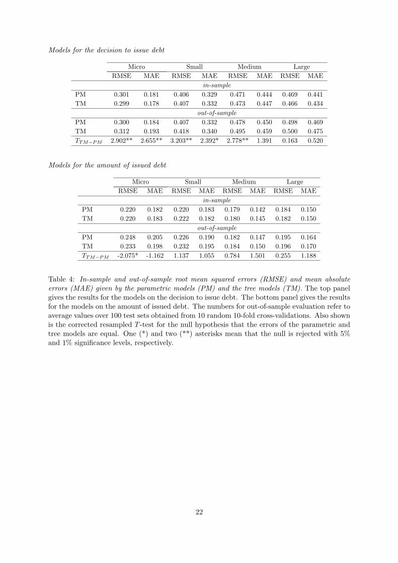
Table 4 shows in-sample and out-of-sample errors of the values predicted by the parametric

models and the tree models. The out-of-sample errors correspond to average values over 100

test sets obtained from 10 random 10-fold cross validations. The corrected resampled T -test

(Nadeau and Bengio, 2003) for the null hypothesis that the prediction errors of the parametric

and tree models are equal is also shown.5 The top panel of Table 4 shows the errors given by

the models for the decision to issue debt. As anticipated, in-sample errors are typically smaller

than out-of-sample errors since the models overfit the data, giving over-optimistic estimates of

the predictive accuracy. Therefore, the models not only fit the “true” relationship between the

5Denote by ε(1)i and ε

(2)i the prediction errors in test set i given by models 1 and 2, respectively, and let

N denote the total number of test sets. The corrected resampled test for the null hypothesis that the mean

errors m(1) = 1N

∑i ε

(1)i and m(2) = 1

N

∑i ε

(2)i are equal is given by T = (m(1) − m(2))/

√(1N

+ q)S, where

S = Var(ε(1) − ε(2)) and q is the ratio between the number of observations in the test set and the numberof observations in the set used for building the models. Here, because 10 random 10-fold cross-validations aregenerated, q = 0.1/0.9 and N = 100. The corrected resampled T -test follows a Student’s t-distribution withN − 1 degrees of freedom.

15

response variable and the explanatory variables but also capture the idiosyncrasies (“noise”)

contained on the data employed in their estimation. Classification tree models exhibit lower

in-sample errors for micro and large firms, while the parametric binary models show better

in-sample accuracies for small and medium firms. On the other hand, the classification trees

have worse out-of-sample errors across the four size-based groups of firms, suggesting that

these models may have lower generalization performance on new data. In terms of RMSE, the

predictive advantage of the parametric models is statistically significant for micro, small and

medium firms, while in terms of MAE it is so for micro and small firm. For large firms, the

differences in errors may be due to sampling variation and the models may have comparable

accuracy.

Table 4 about here

The bottom panel of Table 4 shows the errors given by the models for the amount of issued

debt. Again, the differences between in-sample and out-of-sample errors suggest that both

models overfit the data. The cross-validation suggests that the tree models have better out-of-

sample predictive accuracy, in terms of both RMSE and MAE, for micro firms. On the other

hand, the fractional regression models have lower RMSE and MAE for small, medium and large

firms. The out-of-sample predictive advantage of the tree model over the fractional regression

for micro firms is statistically significant in terms of RMSE at 5% level. On the other hand, the

remaining differences in out-of-sample errors are not statistically significant.

5 Conclusions

This paper analyzes nonparametric decision tree models of financial leverage decisions taken by

micro, small, medium and large sized firms. The study is motivated by the fact that the structure

of these models is not predetermined, as in a parametric approach, but is derived according to

information provided by the data. Also, decision tree predictions are naturally bounded to

the unit interval, respecting the fractional nature of leverage ratios. These appealing features

allowed competing capital structure theories to be tested without making any assumptions with

respect to the conditional expectation of leverage ratios, for the first time in the corporate

finance literature.

This analysis found that parametric two-part models and nonparametric decision trees ex-

hibit several divergencies with respect to which variables are important in financial leverage

decisions. In particular, concerning the decision to issue debt, five instances were identified in

which partial effects are statistically significant in parametric models and absent in tree models.

In seven other cases one finds effects in the tree structures that are not statistically significant

in the parametric models. However, when a variable is significant according to both techniques,

the direction of the partial effect is the same. With respect to decision on the relative amount of

debt to be issued by those firms that do resort to debt, there are five instances in which effects

are identified in the tree models but are not significant in the parametric models. On the other

16

hand, one cannot find significant effects in the parametric models that are not present in the

tree models. This result is rather meaningful, since the tree models for the amount of issued

debt have predictive accuracies comparable to those of the parametric model. Furthermore,

the tree model for micro firms even bestows a statistically significant predictive advantage with

respect to the parametric model.

Overall, the significant relationships found by the tree models are in most cases in accordance

with the effects predicted by the pecking-order theory. Nevertheless, a two-part model can

accommodate better the combined results for the decisions to issue debt and on the amount of

issued debt, since for some groups of firms variables Size and Age have opposite effects on the

two levels of the tree models, while other variables have significant effects only on one of the

two financial leverage decisions analyzed in the paper. This research suggest that an interesting

avenue for future research is the development of a two-part pecking-order theory. For example,

such theory would accommodate straightforwardly the distinct effects of the firm’s age on the

two decisions that was found for micro firms.

References

Bastos, J.A., 2010. Forecasting bank loans loss-given-default. Journal of Banking & Finance 34,

2510-2517.

Breiman, L., Friedman, J.H., Olshen, R.A., Stone, C.J., 1984. Classification and regression

trees. Wadworth International Group, Belmont, California.

Cook, D.O., Kieschnick, R., McCullough, B.D., 2008. Regression analysis of proportions in

finance with self selection. Journal of Empirical Finance 15, 860-867.

Frank, M.Z., Goyal, V.K., 2008. Trade-off and pecking order theories of debt. In: Eckbo, B.E.,

(Ed.), Handbook of Corporate Finance - Empirical Corporate Finance, Elsevier, Amsterdam,

135-202.

Kurshev, A., Strebulaev, I.A., 2007. Firm size and capital structure (Mimeo).

Nadeau, C., Bengio, Y., 2003. Inference for the Generalization Error. Machine Learning 52,

239-281.

Papke, L.E., Wooldridge, J.M., 1996. Econometric methods for fractional response variables

with an application to 401(K) plan participation rates. Journal of Applied Econometrics 11,

619-632.

Quinlan, J.R., 1986. Induction of decision trees. Machine Learning 1, 81-106.

Rajan, R.J., Zingales, L., 1995. What do we know about capital structure? Some evidence from

international data. Journal of Finance 50, 1421-1460.

17

Ramalho, J.J.S. and Silva, J.V., 2009. A two-part fractional regression model for the financial

decisions of micro, small, medium and large firms. Quantitative Finance 9, 621-636.

Ramalho, E.A., J.J.S. Ramalho, Murteira, J.M.R., 2011. Alternative estimating and testing

empirical strategies for fractional regression models. Journal of Economic Surveys, 25(1),

19-68.

Strebulaev, I.A., Yang, B., 2007. The mystery of zero-leverage firms (Mimeo).

Witten, I.H., Frank, E., 2005. Data mining: practical machine learning tools and techniques.

Morgan Kaufmann Publishers.

18

Group Variable Mean Median Min Max St.Dev.

Micro NDTS 0.866 0.503 0.000 102.149 4.039

Tangibility 0.355 0.322 0.000 0.998 0.263

Size 12.063 12.080 6.014 17.215 1.173

Profitability 0.075 0.047 -0.486 1.527 0.118

Growth 17.547 6.436 -81.248 681.354 50.472

Age 16.172 12.000 6.000 110.000 10.003

Liquidity 0.296 0.192 0.000 1.000 0.290

Small NDTS 0.802 0.576 0.000 79.867 2.370

Tangibility 0.420 0.414 0.001 0.996 0.226

Size 13.765 13.715 10.101 17.410 0.972

Profitability 0.062 0.047 -0.161 0.590 0.078

Growth 12.979 6.637 -61.675 267.671 29.444

Age 19.820 17.000 6.000 210.000 13.561

Liquidity 0.175 0.103 0.000 1.000 0.193

Medium NDTS 0.809 0.629 0.000 26.450 1.477

Tangibility 0.466 0.474 0.015 0.979 0.192

Size 15.464 15.446 12.714 18.403 0.909

Profitability 0.055 0.042 -0.109 0.984 0.073

Growth 9.294 4.990 -38.752 188.035 21.671

Age 27.331 22.000 6.000 184.000 18.640

Liquidity 0.124 0.059 0.000 0.963 0.159

Large NDTS 0.902 0.623 0.031 16.327 1.485

Tangibility 0.443 0.462 0.028 0.978 0.203

Size 17.445 17.406 14.741 22.121 1.152

Profitability 0.051 0.035 -0.134 0.441 0.070

Growth 7.451 5.013 -61.621 132.908 18.284

Age 34.203 29.000 5.000 154.000 24.287

Liquidity 0.107 0.053 0.000 0.899 0.140

Table 1: Descriptive statistics of the explanatory variables according to the size-based groups offirms.

19

Variable Micro Small Medium Large

PM TM PM TM PM TM PM TMNDTS • • • • • • • •Tangibility • − (214) + • + + (229) • + (271)Size + + (1446) + + (454) + + (851) • •Profitability • • − − (1951) − − (1024) • •Growth • + (41) • + (481) + • • + (221)Age • + (236) • • • • • •Liquidity − • − − (1752) − − (726) • •Manufacturing • • • + (768) • • • •Construction • • • • • • • •Trade − − (311) • • − • • •Transport − − (282) − • • • • •No. Observations 1446 1951 1024 271

Table 2: Effects of explanatory variables for the probability of issuing debt based on parametricmodels (PM) and tree models (TM). The figure in parentesis indicates the number of firms forwhich the effect is relevant. Relevant effects are classified as positive (+) or negative (−). Abullet (•) indicates that a variable is irrelevant in explaining the probability of issuing debt.

20

Variable Micro Small Medium Large

PM TM PM TM PM TM PM TMNDTS • + (114) • • • − (399) − − (117)Tangibility • • • − (452) • • • •Size • • − − (36) − − (101) • •Profitability • • • − (143) − − (500) − − (161)Growth • • • • • • • •Age • − (52) − − (357) • • • •Liquidity • • • • • • • •Manufacturing • • • • • • • •Construction + + (164) + + (95) • • • •Trade • • • • • • • •Transport • • • • • • • •No. Observations 164 452 500 161

Table 3: Effects of explanatory variables for the amount of issued debt based on parametricmodels (PM) and tree models (TM). The figure in parentesis indicates the number of firms forwhich the effect is relevant. Relevant effects are classified as positive (+) or negative (-). Abullet (•) indicates that a variable is irrelevant in explaining the amount of issued debt.

21

Models for the decision to issue debt

Micro Small Medium Large

RMSE MAE RMSE MAE RMSE MAE RMSE MAE

in-sample

PM 0.301 0.181 0.406 0.329 0.471 0.444 0.469 0.441

TM 0.299 0.178 0.407 0.332 0.473 0.447 0.466 0.434

out-of-sample

PM 0.300 0.184 0.407 0.332 0.478 0.450 0.498 0.469

TM 0.312 0.193 0.418 0.340 0.495 0.459 0.500 0.475

TTM−PM 2.902** 2.655** 3.203** 2.392* 2.778** 1.391 0.163 0.520

Models for the amount of issued debt

Micro Small Medium Large

RMSE MAE RMSE MAE RMSE MAE RMSE MAE

in-sample

PM 0.220 0.182 0.220 0.183 0.179 0.142 0.184 0.150

TM 0.220 0.183 0.222 0.182 0.180 0.145 0.182 0.150

out-of-sample

PM 0.248 0.205 0.226 0.190 0.182 0.147 0.195 0.164

TM 0.233 0.198 0.232 0.195 0.184 0.150 0.196 0.170

TTM−PM -2.075* -1.162 1.137 1.055 0.784 1.501 0.255 1.188

Table 4: In-sample and out-of-sample root mean squared errors (RMSE) and mean absoluteerrors (MAE) given by the parametric models (PM) and the tree models (TM). The top panelgives the results for the models on the decision to issue debt. The bottom panel gives the resultsfor the models on the amount of issued debt. The numbers for out-of-sample evaluation refer toaverage values over 100 test sets obtained from 10 random 10-fold cross-validations. Also shownis the corrected resampled T -test for the null hypothesis that the errors of the parametric andtree models are equal. One (*) and two (**) asterisks mean that the null is rejected with 5%and 1% significance levels, respectively.

22

root node

x < c x > ciii i

x < c jj x < ckkx > cj j x > ck k

Figure 1: Simple scheme of a decision tree model. The model is represented by a sequence oflogical if-then-else tests on the attributes of the observations. The terminal nodes, denoted byleaves, are depicted by rectangles.

23

<0.233 >0.233

<-2.450 >-2.450

no debt

no debt debt

Tangibility?

Growth?

MICRO FIRMS SMALL FIRMS

no debt

no debt

no debt

no debt

no debt

debt

debt debt

no debt

no debt

no debt

no debt

no debt

no debt

noyes

yes no no yes

Size?

Size?

Size?

Growth?

Growth?

Liquidity?

Liquidity?

Liquidity?

Age?

Tangibility?

Trade?

Transport?

Profitability?

Manufacturing?

no debt

no debt debt

LARGE FIRMS

>12.923<12.923

<25

<0.026

<18.478

<0.145

<0.073

<-15.692

<14.522

<0.047

<0.086

<14.216

<0.165

>25

>0.026

>18.478

>0.073

>0.145

>-15.692

>14.522

>0.047

>0.086

>14.216

>0.165

1052:83

35:11

139:34

27:2

9:13

225:364

15:9

53:16

83:54

5:12

186:13

791:193

196:91

26:1

257:100

18:625:48

33:17

30:26 47:118135:38

Profitability?

Tangibility?

<0.550>0.550

MEDIUM FIRMS

no debt

18:7

Size?

no debt

<15.456 >15.456

10:21

debt

Figure 2: Classification tree models for the decision to issue debt.

24

Construction?

Tangibility?Construction?

NDTS?

Age?

Age?

Profitability?

Size?

Profitability?

NDTS? Size?

Profitability?

NDTS?

0.6083

0.4501

0.2894 0.3560

yes no

>0.512

>20.5 <20.5

<0.512 yes no >19.5 <19.5

<0.057 >0.057

>13.547 <13.547

0.5322 0.4039 0.3969

0.3391

0.2164 0.2747

<0.072 >0.072

<0.548 >0.548 <15.561 >15.561

<0.064>0.064

<0.573 >0.573

0.3667 0.3000 0.2983 0.2095

0.1983

0.3512 0.2589

MICRO FIRMS SMALL FIRMS

MEDIUM FIRMS LARGE FIRMS

62

50

15 37

47 48 214

107

28 8

44

25 92574430891

<0.265 >0.265

Figure 3: Regression tree models for the amount of issued debt.

25