Embed Size (px)
Citation preview

The financial conglomerate discount: Insights
from stock return skewness
September 9, 2018
Abstract
The value of financial conglomerates is often discounted than comparable combi-nations of stand-alone firms. This article explores the hypothesis that expected stockreturns contribute significantly to determine this puzzle. In order to approximate thefuture returns, we measure the skewness of stock returns. The main finding is thatdiversified banks are largely discounted when their stock returns are less skewed thancomparable undiversified firms. This evidence is line with the argument that businessdiversification destroys upside potential, to the extent that investors expect to receivehigher returns from diversified banks than from comparables. The outcomes inte-grate the existing interpretation for the financial conglomerate discount by drawingattention on the role of expected returns for corporate valuation.
Keywords: financial conglomerates; discount; expected returns; skewness
JEL classification: G21; G32
1 Introduction and review of the literature
The corporate value of financial conglomerates is frequently observed to be discounted in
respect to the aggregate value of comparable portfolios of stand-alone firms. This fact is
known in the literature as the “financial conglomerate discount” and is seen as a puzzle,
which has not received yet an exhaustive interpretation. In fact, this evidence brings to
the conclusion that corporate value would increase if conglomerates got dismantled. In
other words, business diversification would destroy value to banking corporations.1
1Some articles refer to this issue as the“diversification discount” rather than “conglomerate discount,”so to emphasize the perverse effect of business diversification for corporate valuation. Throughout thispaper, when we quote papers on this subject, we will not make a distinction between the two headings andwill use the term “financial conglomerate discount.”Maksimovic and Phillips (2013) provide an overviewof the literature dealing with the conglomerate discount inside non-financial industries. However, theempirical evidence is still quite mixed, as for example Campa and Kedia (2002) and Villalonga (2004)obtain results that do not confirm the existence of the conglomerate discount.
1
Among others, Laeven and Levine (2007) show that diversified banks that engage
into lending and non-lending services are discounted compared to undiversified banks.
The authors do not identify the causal factors, but they suggest that the discount would
arise from agency conflicts that would be especially severe inside large diversified banks.
Schmid and Walter (2009) reveals the existence of a persistent conglomerate discount for
several types of corporate structures taken by large and diversified financial intermedi-
aries. Van Lelyveld and Knot (2009) show that the discount attached to bank-insurance
conglomerates is correlated to their size, risk profile, and the familiarity of investors with
the conglomerate business model. Stiroh and Rumble (2006) contend that one “dark side”
of diversification inside financial holding companies (FHCs) is to increase their exposure
to volatile activities, with consequences for the firm value through missed investment
opportunities and increased costs.2
The banking literature on this topic is quite limited. The articles cited above agree in
documenting the existence of the conglomerate discount, but they do not study exhaus-
tively the determinants for such puzzle. The previous articles that analyze non-financial
conglomerates have mainly explained the so-called “cash flow portion” of the discount
by showing that business diversification reduces cash flows introducing distortions like
capital mis-allocation (Lang et al., 1994; Berger and Ofek, 1995) and agency problems
(Lins and Servaes, 1999; Denis et al., 1997). However, there would be also the “expected
return portion” to consider (Lamont and Polk, 2001). In fact, assessing corporate value
requires to discount the future cash flows at an opportunity rate that reflects the risk of
the investment.3 Expected returns - likewise cash flows - are key elements for corporate
valuation. Few papers in the literature hint that investors may not be able to fairly assess
conglomerates. Van Lelyveld and Knot (2009) argue that irrational investors end up to
mis-price complex and opaque conglomerates, in line with the discussion in Hadlock et al.
(1999). Saunders and Walter (2012) maintain that both universal banks and financial
conglomerates bear discounts that origin from capital mis-allocation as well as portfolio-
2The question whether financial conglomerates on average trade at a discount remains not solvedentirely, since there is evidence that diversification improves the performance of financial conglomerates,as for example Baele et al. (2007) and Elsas et al. (2010).
3The discounted cash flow methodology is explained in more depth from Ross et al. (2011), amongothers.
2
selection effects, due to investors that are not able to “take the view” of complex corporate
structures while they prefer to remain undiversified. The above papers corroborate the
idea that it would be meaningful to investigate expected returns in order to understand
more precisely the valuation of financial conglomerates. Nonetheless, until now we could
not find empirical research that corroborates this claim. Instead, the aim of this article
is to provide quantitative evidence for the argument that we can interpret the financial
conglomerate puzzle by casting attention on the role of expected returns for corporate
valuation.
We analyze banks in the United States during 2005-2017 and use the skewness of
stock returns in order to identify bank expected returns, thereby following the stream of
research that argues that stock return skewness reveals information on future expected
performance.4 The argument is that stocks with right-tailed returns have higher proba-
bility of benefiting from huge gains than of suffering from huge losses, therefore investors,
ceteris paribus, prefer assets with positive skewness and demand higher expected returns
to negatively skewed stocks in order to compensate the risk of bad performance. We fol-
low the approach of Lang et al. (1994) and Berger and Ofek (1995), among others, that is
known as “chop shop.” This methodology requires that we construct for each diversified
bank of the sample a comparable combination of stand-alone firms. The main idea is to
compare the value of the bank to the value of the mimicking portfolio of firms. The dif-
ference between the two quantities approximates the size of the discount attached to the
conglomerate; i.e. the bank is asserted as discounted if it has lower value than its mim-
icking portfolio. Corporate value is measured primarily with Tobins’q, see Laeven and
Levine (2007). Instrumental variable regressions show that the value of diversified banks
is substantially lower than the value of comparable undiversified firms when their expected
returns are higher than the returns of the comparables. This evidence is in line with the
hypothesis that business diversification subtracts upside potential. As a consequence of
4The seminal papers advancing the hypothesis that skewness and expected returns are inversely relatedare Arditti (1967) and Scott and Horvath (1980). The empirical evidence remains though mixed. Forexample, Brunnermeier et al. (2007) and Barberis and Huang (2008) provide a theoretical framework thatjustifies the link between skewness and expected returns. Among others, the correlation between skewnessand expected returns is negative in the articles of Mitton and Vorkink (2007), Bali and Murray (2013) andConrad et al. (2013), while it is positive in the articles of Stilger et al. (2016) and Bali et al. (2017).
3
the worse prospects, investors demand higher returns from diversified banks rather than
from comparable combinations of single-segment firms. In fact, investors will hold finan-
cial conglomerates only if they get a discount, otherwise they will remain undiversified
and buy separately the conglomerate units.
The results are robust to the computation of both sample-based skewness (Mitton and
Vorkink, 2007, 2010; Boyer et al., 2010; Del Viva et al., 2017), as well as option-implied
skewness (Malz, 2014). The main advantage of using option-implied moments is that they
are forward-looking quantities, i.e they are more consistent with the concept of expected
returns (Chang et al., 2013; Conrad et al., 2013). We further verify the link between
skewness and realized (i.e. ex-post) stock returns. In fact, under the rational expectation
hypothesis, on average the realized ex-post stock returns correspond to the ex-ante required
returns. In our sample realized returns and skewness correlate negatively, implying that
rational investors accept lower expected returns for right-skewed stocks. Furthermore,
additional asset pricing tests detect that bank stock returns entail a premium for negative
skewness.
The set of outcomes confirm that a substantial share of the financial conglomerate dis-
count is driven by interactions arising between business diversification and future returns.
This statement adds to the current wisdom that frictions within the cash flow management
of large corporations are the main responsible for the driver of conglomerate discount
The article proceeds as follows. Section 2 introduces the sample and the main variables
that we use in the analysis. Section 3 performs empirical tests in order to verify the
hypothesis that diversified banks trade at a discount compared to portfolios of stand-
alone firms because of differences in the expected returns explained by skewness-based
measures. Section 4 conducts robustness tests. Section 5 concludes.
2 Sample and variables
2.1 Sample
S&P Global Market Intelligence Platform provides quarterly accounting and market based
data for financial companies classified as “bank” in the United States during the time
4
span 2005q1-2017q4. The series of monthly stock prices are downloaded from Thomson
Reuters Datastream. Table 1 reports descriptive statistics for the variables of the empirical
analysis. The goal is to illustrate that expected returns contribute significantly to the
discount attached to diversified banks.
2.2 Excess value
The vast majority of the literature studies the conglomerate discount implementing the so-
called “chop-shop” approach, initiated by LeBaron and Speidell (1987), Lang et al. (1994),
and Berger and Ofek (1995). The idea is to replicate the conglomerate by constructing
a portfolio of stand-alone firms in such a way that the conglomerate and the portfolio
offer a similar degree of business diversification. If a conglomerate is worth less than
the comparable portfolio, then we identify the conglomerate as discounted. This finding
implies that value would increase if the conglomerate got dismantled, namely when the
units are independent and do not form a unique corporation.
We cannot apply the “chop-shop” approach straightforward to our banks, because in
the database we cannot find their number of divisions or segments. To deal with this
issue, we follow Laeven and Levine (2007), who analyze data of financial conglomerates.
For each firm j we define the excess value as the difference between the Tobin’s q and the
imputed “activity adjusted” Tobin’s q.5 Tobin’s q is the sum of common equity market
value, book value of preferred shares, and book value of total debt divided by book value
of total assets. Using Tobin’s q has the important advantage that we can compare value
across firms without needing to adjust for risk or leverage, as motivated by Lang et al.
(1994) and Laeven and Levine (2007).
We define the Tobin’s q imputed to bank j as the value attached to a portfolio made by
a specialized commercial bank and a specialized investment bank. The weight of the two
firms inside the portfolio is proportional to the loans-to-assets ratio α of the conglomerate
5Lang et al. (1994) and Berger and Ofek (1995) are the seminal papers that find evidence for theconglomerate discount by testing the Tobin’s q of firms. More recently Laeven and Levine (2007) usesTobin’s q to analyze financial conglomerates. Mitton and Vorkink (2010) analyzes the company excessvalue by taking the natural logarithm of Tobin’s q. Given that inside our sample the distribution of thevariable for Tobin’s q is not very highly skewed, we prefer to report the regression results obtained as usingthe point value of Tobin’s q. Our results do not change qualitatively when we use the log-value.
5
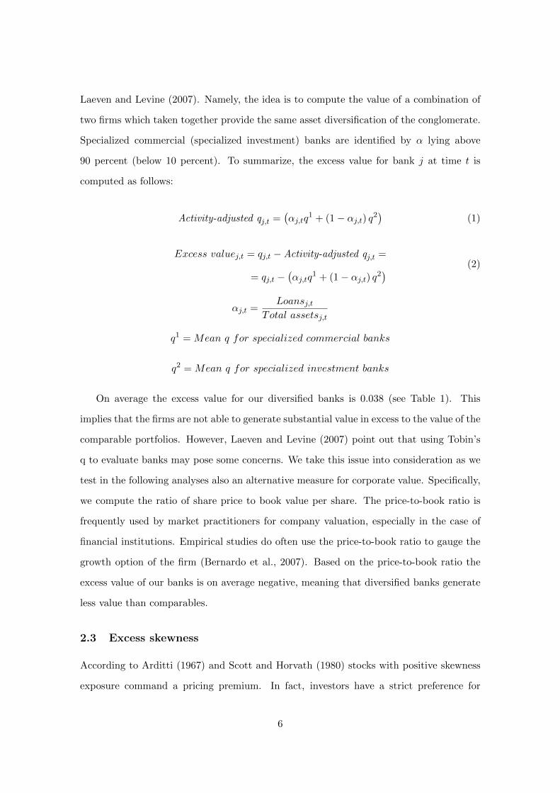
Laeven and Levine (2007). Namely, the idea is to compute the value of a combination of
two firms which taken together provide the same asset diversification of the conglomerate.
Specialized commercial (specialized investment) banks are identified by α lying above
90 percent (below 10 percent). To summarize, the excess value for bank j at time t is
computed as follows:
Activity-adjusted qj,t =(αj,tq
1 + (1− αj,t) q2)
(1)
Excess valuej,t = qj,t −Activity-adjusted qj,t =
= qj,t −(αj,tq
1 + (1− αj,t) q2) (2)
αj,t =Loansj,t
Total assetsj,t
q1 = Mean q for specialized commercial banks
q2 = Mean q for specialized investment banks
On average the excess value for our diversified banks is 0.038 (see Table 1). This
implies that the firms are not able to generate substantial value in excess to the value of the
comparable portfolios. However, Laeven and Levine (2007) point out that using Tobin’s
q to evaluate banks may pose some concerns. We take this issue into consideration as we
test in the following analyses also an alternative measure for corporate value. Specifically,
we compute the ratio of share price to book value per share. The price-to-book ratio is
frequently used by market practitioners for company valuation, especially in the case of
financial institutions. Empirical studies do often use the price-to-book ratio to gauge the
growth option of the firm (Bernardo et al., 2007). Based on the price-to-book ratio the
excess value of our banks is on average negative, meaning that diversified banks generate
less value than comparables.
2.3 Excess skewness
According to Arditti (1967) and Scott and Horvath (1980) stocks with positive skewness
exposure command a pricing premium. In fact, investors have a strict preference for
6
positive skewness. When stock returns are positively skewed, the distribution has more
mass for large positive outcomes than for large negative outcomes, meaning that it is more
likely that the firm will benefit from positive gains than suffering losses. The consequence is
that investors will pay a premium for assets entailing positive return skewness. In contrast,
negative skewness indicates a high probability of shortfalls. Investors will incur downside
potential only for a pricing discount, in order to be compensated by higher expected
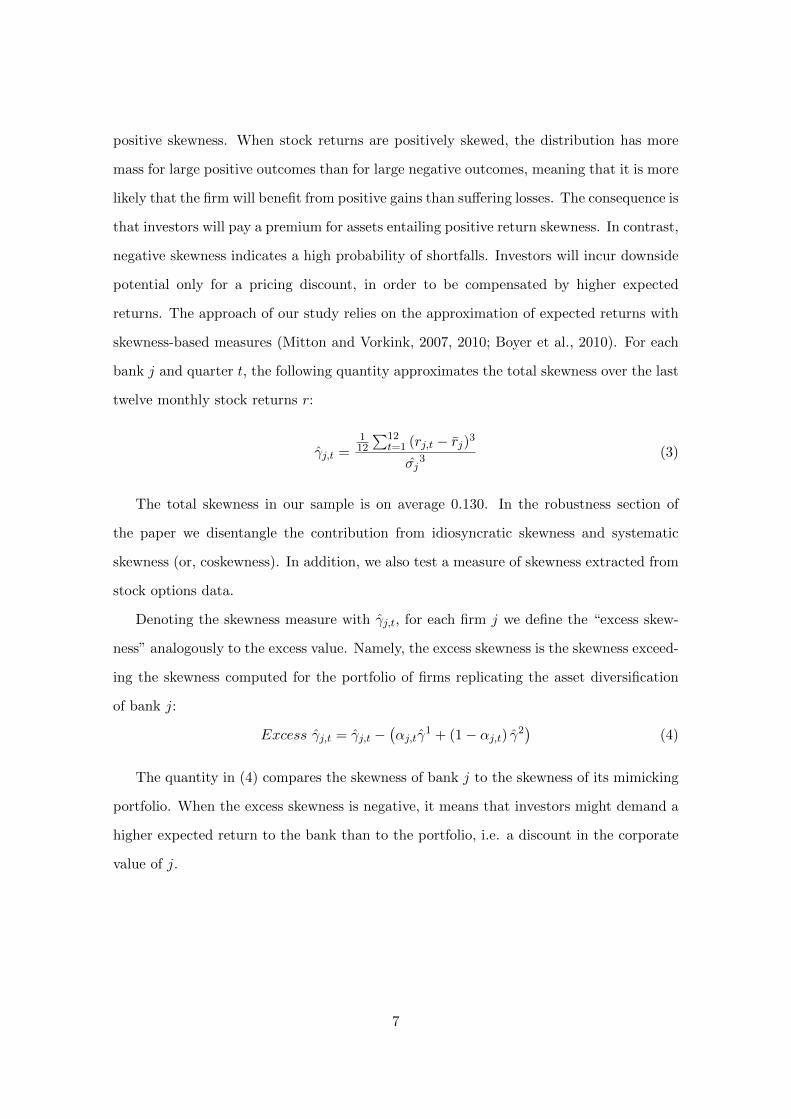
returns. The approach of our study relies on the approximation of expected returns with
skewness-based measures (Mitton and Vorkink, 2007, 2010; Boyer et al., 2010). For each
bank j and quarter t, the following quantity approximates the total skewness over the last
twelve monthly stock returns r:
γj,t =112
∑12t=1 (rj,t − rj)3
σj3 (3)
The total skewness in our sample is on average 0.130. In the robustness section of
the paper we disentangle the contribution from idiosyncratic skewness and systematic
skewness (or, coskewness). In addition, we also test a measure of skewness extracted from
stock options data.
Denoting the skewness measure with γj,t, for each firm j we define the “excess skew-
ness” analogously to the excess value. Namely, the excess skewness is the skewness exceed-
ing the skewness computed for the portfolio of firms replicating the asset diversification
of bank j:
Excess γj,t = γj,t −(αj,tγ
1 + (1− αj,t) γ2)
(4)
The quantity in (4) compares the skewness of bank j to the skewness of its mimicking
portfolio. When the excess skewness is negative, it means that investors might demand a
higher expected return to the bank than to the portfolio, i.e. a discount in the corporate
value of j.
7
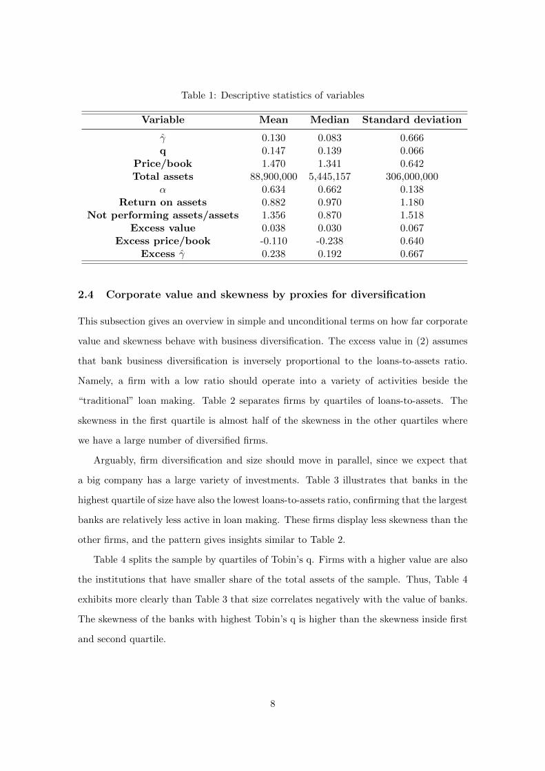
Table 1: Descriptive statistics of variables
Variable Mean Median Standard deviation
γ 0.130 0.083 0.666q 0.147 0.139 0.066
Price/book 1.470 1.341 0.642Total assets 88,900,000 5,445,157 306,000,000
α 0.634 0.662 0.138Return on assets 0.882 0.970 1.180
Not performing assets/assets 1.356 0.870 1.518Excess value 0.038 0.030 0.067
Excess price/book -0.110 -0.238 0.640Excess γ 0.238 0.192 0.667
2.4 Corporate value and skewness by proxies for diversification
This subsection gives an overview in simple and unconditional terms on how far corporate
value and skewness behave with business diversification. The excess value in (2) assumes
that bank business diversification is inversely proportional to the loans-to-assets ratio.
Namely, a firm with a low ratio should operate into a variety of activities beside the
“traditional” loan making. Table 2 separates firms by quartiles of loans-to-assets. The
skewness in the first quartile is almost half of the skewness in the other quartiles where
we have a large number of diversified firms.
Arguably, firm diversification and size should move in parallel, since we expect that
a big company has a large variety of investments. Table 3 illustrates that banks in the
highest quartile of size have also the lowest loans-to-assets ratio, confirming that the largest
banks are relatively less active in loan making. These firms display less skewness than the
other firms, and the pattern gives insights similar to Table 2.
Table 4 splits the sample by quartiles of Tobin’s q. Firms with a higher value are also
the institutions that have smaller share of the total assets of the sample. Thus, Table 4
exhibits more clearly than Table 3 that size correlates negatively with the value of banks.
The skewness of the banks with highest Tobin’s q is higher than the skewness inside first
and second quartile.
8
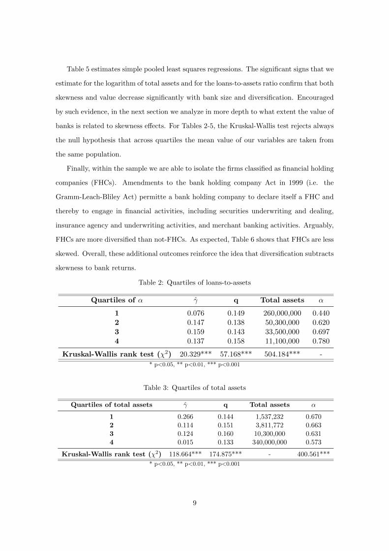
Table 5 estimates simple pooled least squares regressions. The significant signs that we
estimate for the logarithm of total assets and for the loans-to-assets ratio confirm that both
skewness and value decrease significantly with bank size and diversification. Encouraged
by such evidence, in the next section we analyze in more depth to what extent the value of
banks is related to skewness effects. For Tables 2-5, the Kruskal-Wallis test rejects always
the null hypothesis that across quartiles the mean value of our variables are taken from
the same population.
Finally, within the sample we are able to isolate the firms classified as financial holding
companies (FHCs). Amendments to the bank holding company Act in 1999 (i.e. the
Gramm-Leach-Bliley Act) permitte a bank holding company to declare itself a FHC and
thereby to engage in financial activities, including securities underwriting and dealing,
insurance agency and underwriting activities, and merchant banking activities. Arguably,
FHCs are more diversified than not-FHCs. As expected, Table 6 shows that FHCs are less
skewed. Overall, these additional outcomes reinforce the idea that diversification subtracts
skewness to bank returns.
Table 2: Quartiles of loans-to-assets
Quartiles of α γ q Total assets α
1 0.076 0.149 260,000,000 0.4402 0.147 0.138 50,300,000 0.6203 0.159 0.143 33,500,000 0.6974 0.137 0.158 11,100,000 0.780
Kruskal-Wallis rank test (χ2) 20.329*** 57.168*** 504.184*** -
* p<0.05, ** p<0.01, *** p<0.001
Table 3: Quartiles of total assets
Quartiles of total assets γ q Total assets α
1 0.266 0.144 1,537,232 0.6702 0.114 0.151 3,811,772 0.6633 0.124 0.160 10,300,000 0.6314 0.015 0.133 340,000,000 0.573
Kruskal-Wallis rank test (χ2) 118.664*** 174.875*** - 400.561***
* p<0.05, ** p<0.01, *** p<0.001
9
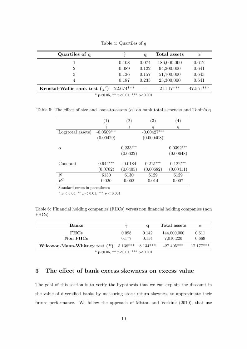
Table 4: Quartiles of q
Quartiles of q γ q Total assets α
1 0.108 0.074 186,000,000 0.6122 0.089 0.122 94,300,000 0.6413 0.136 0.157 51,700,000 0.6434 0.187 0.235 23,300,000 0.641
Kruskal-Wallis rank test (χ2) 22.674*** - 21.117*** 47.551***
* p<0.05, ** p<0.01, *** p<0.001
Table 5: The effect of size and loans-to-assets (α) on bank total skewness and Tobin’s q
(1) (2) (3) (4)γ γ q q
Log(total assets) -0.0509∗∗∗ -0.00427∗∗∗
(0.00429) (0.000408)
α 0.233∗∗∗ 0.0392∗∗∗
(0.0622) (0.00648)
Constant 0.944∗∗∗ -0.0184 0.215∗∗∗ 0.122∗∗∗
(0.0702) (0.0405) (0.00682) (0.00411)
N 6130 6130 6129 6129R2 0.020 0.002 0.014 0.007
Standard errors in parentheses∗ p < 0.05, ∗∗ p < 0.01, ∗∗∗ p < 0.001
Table 6: Financial holding companies (FHCs) versus non financial holding companies (nonFHCs)
Banks γ q Total assets α
FHCs 0.098 0.142 144,000,000 0.611Non FHCs 0.177 0.154 7,010,220 0.669
Wilcoxon-Mann-Whitney test (F ) 5.138*** 8.134*** -27.405*** 17.177***
* p<0.05, ** p<0.01, *** p<0.001
3 The effect of bank excess skewness on excess value
The goal of this section is to verify the hypothesis that we can explain the discount in
the value of diversified banks by measuring stock return skewness to approximate their
future performance. We follow the approach of Mitton and Vorkink (2010), that use
10

instrumental variable regressions to relate firm excess value to excess skewness. More
precisely, we estimate the following panel regression model in two steps:
Excess valuej,t = β0 + β1Excess skewness∗j,t + θXj,t+ νt+ υj+ εj,t (5)
where the excess value of bank j for quarter t is regressed on the excess skewness for
the same quarter. Xj,t is the vector of instruments that includes the logarithm of total
assets, the return-on-assets, and the ratio of not performing assets over assets. νt and υj
capture time and bank fixed effects, as they control for potential time-invariant and firm-
specific characteristics that could bias the outcomes. The error term of the regression is
denoted with εj,t. The excess skewness∗j,t is the series of values predicted by a preliminary
estimation where the excess skewness for quarter t is made regress on the t− 1 skewness
and stock return Mitton and Vorkink (2010):
Excess skewnessj,t = α0 + α1Skewnessj,t−1 + α2rj,t−1 + τ t+ψj+ωj,t (6)
The linear prediction from the fitted model (6) provides the excess skewness at t as
predicted on the base of the t−1 variables. This prediction enters as explanatory variable
into (5).
Table 7 shows that the estimated coefficient β1 is positive and significant. The magni-
tude of this effect is higher for the price-to-book ratio. This evidence confirms the working
argument that the value of diversified banks is more largely discounted as long as their
expected returns increase, i.e. our outcomes for banks are in line with Mitton and Vorkink
(2010) for non-financial firms.
11

Table 7: The effect of excess skewness on bank excess value
(1) (2)Excess value Excess price/book
Excess γ 0.0108∗∗∗ 0.129∗∗∗
(0.00124) (0.0115)
Log(total assets) -0.0147∗∗∗ -0.314∗∗∗
(0.00157) (0.0146)
Return on assets 0.00785∗∗∗ 0.0409∗∗∗
(0.000487) (0.00455)
Not performing assets/assets -0.0180∗∗∗ -0.205∗∗∗
(0.000478) (0.00447)
Constant 0.286∗∗∗ 5.031∗∗∗
(0.0248) (0.231)
Bank fixed effects Yes Yes
Time fixed effects Yes Yes
N 5434 5432R2 0.292 0.353
Standard errors in parentheses∗ p < 0.05, ∗∗ p < 0.01, ∗∗∗ p < 0.001
4 Robustness Tests
4.1 Idiosyncratic skewness and coskewness
Total skewness can be decomposed into idiosyncratic skewness and coskewness (or, system-
atic skewness). In principle, both components should matter for asset pricing, although
there is no clear evidence if one of the two is predominant.6. Coskewness measures the
amount of covariance with the squared market return that a security’s returns adds to
the investor’s portfolio. Positive coskewness tells whether both the stock and the market
portfolio undergo extreme positive deviations at the same time. According to the seminal
paper of Kraus and Litzenberger (1976), market valuations incorporate only coskewness.
6Boyer et al. (2010) show that stock returns are negatively correlated with expected idiosyncraticskewness, in line with the theories in Mitton and Vorkink (2007), Brunnermeier et al. (2007), Barberis andHuang (2008), Brunnermeier and Parker (2005)
12
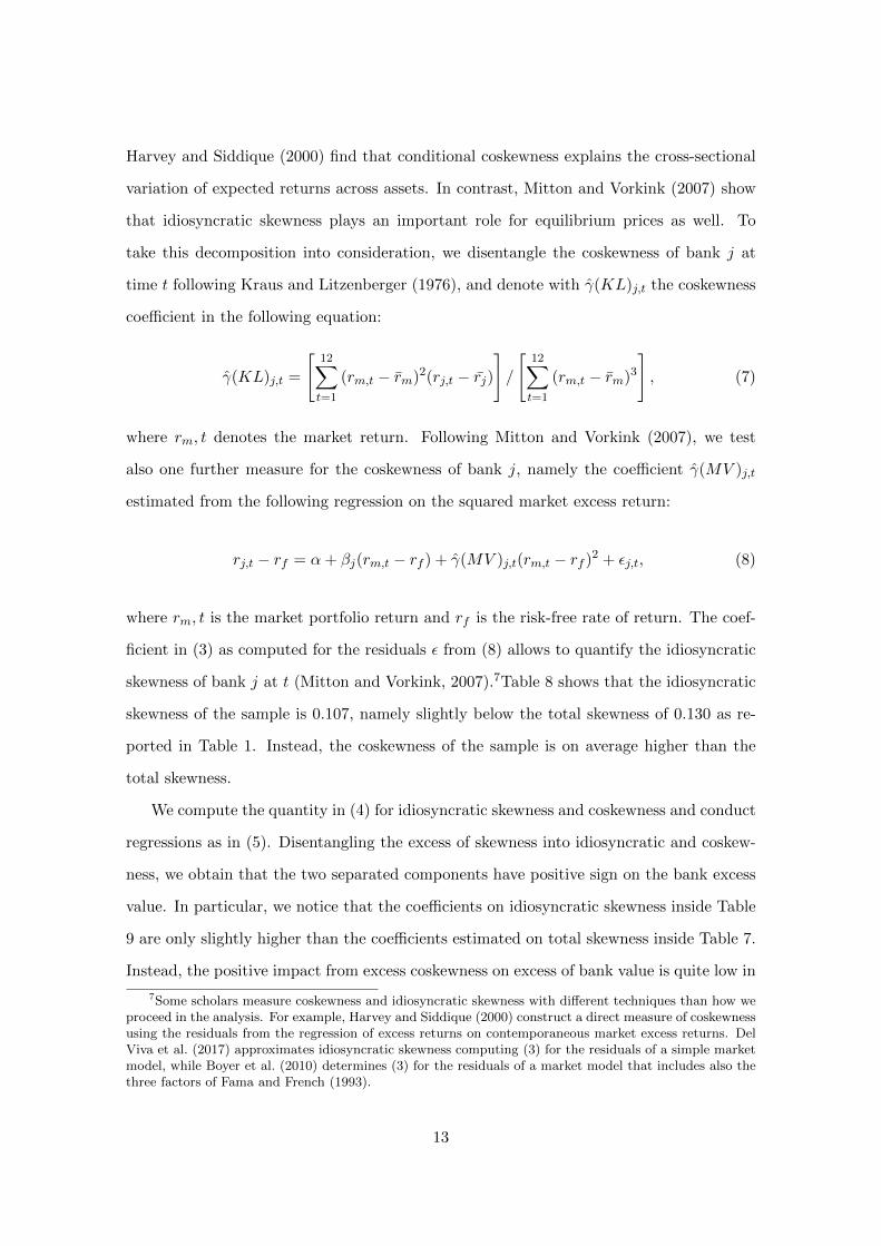
Harvey and Siddique (2000) find that conditional coskewness explains the cross-sectional
variation of expected returns across assets. In contrast, Mitton and Vorkink (2007) show
that idiosyncratic skewness plays an important role for equilibrium prices as well. To
take this decomposition into consideration, we disentangle the coskewness of bank j at
time t following Kraus and Litzenberger (1976), and denote with γ(KL)j,t the coskewness
coefficient in the following equation:
γ(KL)j,t =
[12∑t=1
(rm,t − rm)2(rj,t − rj)
]/
[12∑t=1
(rm,t − rm)3
], (7)
where rm, t denotes the market return. Following Mitton and Vorkink (2007), we test
also one further measure for the coskewness of bank j, namely the coefficient γ(MV )j,t
estimated from the following regression on the squared market excess return:
rj,t − rf = α+ βj(rm,t − rf ) + γ(MV )j,t(rm,t − rf )2 + εj,t, (8)
where rm, t is the market portfolio return and rf is the risk-free rate of return. The coef-
ficient in (3) as computed for the residuals ε from (8) allows to quantify the idiosyncratic
skewness of bank j at t (Mitton and Vorkink, 2007).7Table 8 shows that the idiosyncratic
skewness of the sample is 0.107, namely slightly below the total skewness of 0.130 as re-
ported in Table 1. Instead, the coskewness of the sample is on average higher than the
total skewness.
We compute the quantity in (4) for idiosyncratic skewness and coskewness and conduct
regressions as in (5). Disentangling the excess of skewness into idiosyncratic and coskew-
ness, we obtain that the two separated components have positive sign on the bank excess
value. In particular, we notice that the coefficients on idiosyncratic skewness inside Table
9 are only slightly higher than the coefficients estimated on total skewness inside Table 7.
Instead, the positive impact from excess coskewness on excess of bank value is quite low in
7Some scholars measure coskewness and idiosyncratic skewness with different techniques than how weproceed in the analysis. For example, Harvey and Siddique (2000) construct a direct measure of coskewnessusing the residuals from the regression of excess returns on contemporaneous market excess returns. DelViva et al. (2017) approximates idiosyncratic skewness computing (3) for the residuals of a simple marketmodel, while Boyer et al. (2010) determines (3) for the residuals of a market model that includes also thethree factors of Fama and French (1993).
13

absolute terms, although still statistically significant. The conclusion is that the baseline
results that we get for total skewness are mainly driven by idiosyncratic skewness.
Table 8: Descriptive statistics of variables for idiosyncratic skewness and coskewness (KLand MV)
Variable Mean Median
γ(idiosyncratic) 0.107 0.092γ(KL) 1.237 1.030γ(MV ) 0.793 -0.175
Excess γ(idiosyncratic) 0.100 0.084Excess γ(KL) 0.104 0.065Excess γ(MV ) 2.388 0.606
Table 9: The effect of excess idiosyncratic skewness on bank excess value
(1) (2)Excess value Excess price/book
Excess γ(idiosyncratic) 0.0140∗∗∗ 0.173∗∗∗
(0.00193) (0.0181)
Log(total assets) -0.0134∗∗∗ -0.298∗∗∗
(0.00160) (0.0149)
Return on assets 0.00790∗∗∗ 0.0415∗∗∗
(0.000493) (0.00462)
Not performing assets/assets -0.0178∗∗∗ -0.203∗∗∗
(0.000483) (0.00453)
Constant 0.266∗∗∗ 4.784∗∗∗
(0.0253) (0.237)
Bank fixed effects Yes Yes
Time fixed effects Yes Yes
N 5434 5432R2 0.276 0.332
Standard errors in parentheses∗ p < 0.05, ∗∗ p < 0.01, ∗∗∗ p < 0.001
14
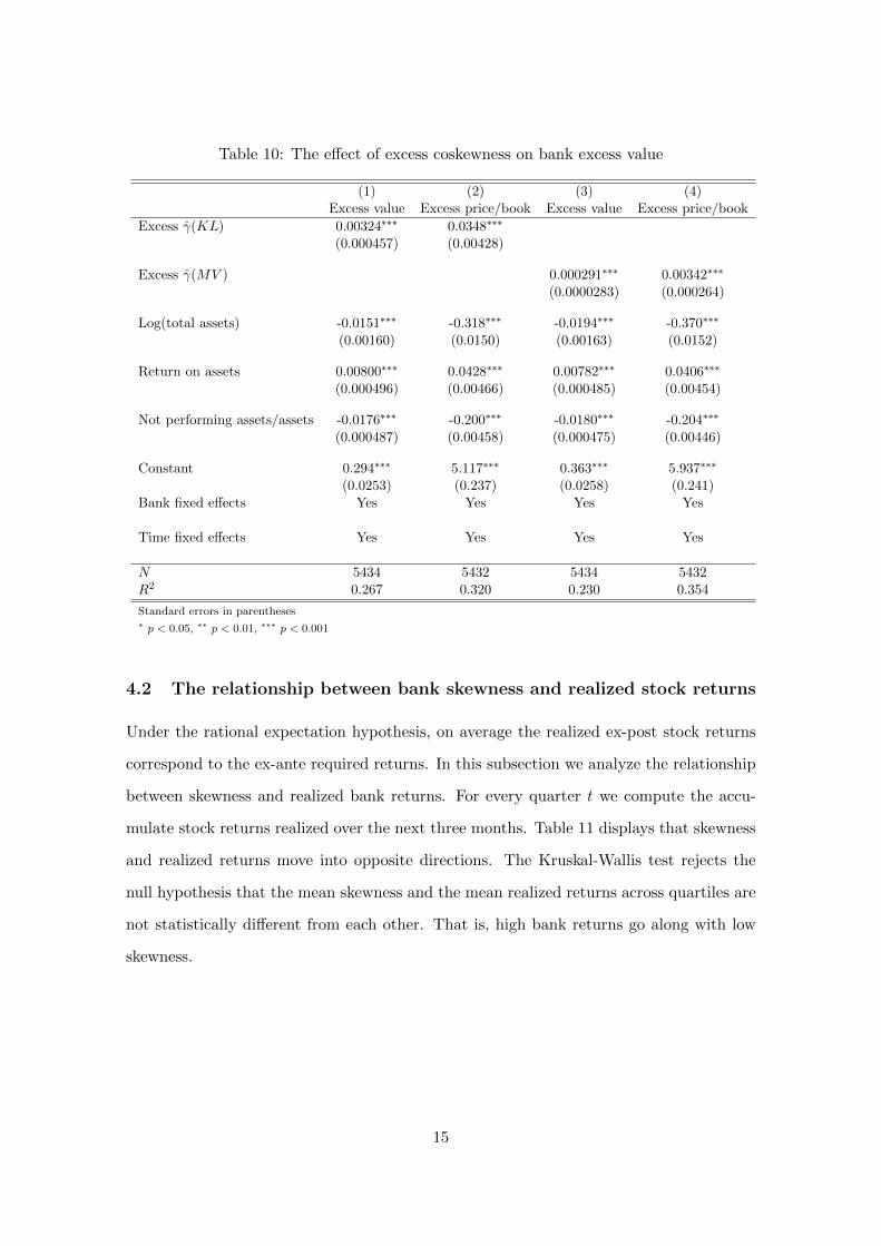
Table 10: The effect of excess coskewness on bank excess value
(1) (2) (3) (4)Excess value Excess price/book Excess value Excess price/book
Excess γ(KL) 0.00324∗∗∗ 0.0348∗∗∗
(0.000457) (0.00428)
Excess γ(MV ) 0.000291∗∗∗ 0.00342∗∗∗
(0.0000283) (0.000264)
Log(total assets) -0.0151∗∗∗ -0.318∗∗∗ -0.0194∗∗∗ -0.370∗∗∗
(0.00160) (0.0150) (0.00163) (0.0152)
Return on assets 0.00800∗∗∗ 0.0428∗∗∗ 0.00782∗∗∗ 0.0406∗∗∗
(0.000496) (0.00466) (0.000485) (0.00454)
Not performing assets/assets -0.0176∗∗∗ -0.200∗∗∗ -0.0180∗∗∗ -0.204∗∗∗
(0.000487) (0.00458) (0.000475) (0.00446)
Constant 0.294∗∗∗ 5.117∗∗∗ 0.363∗∗∗ 5.937∗∗∗
(0.0253) (0.237) (0.0258) (0.241)Bank fixed effects Yes Yes Yes Yes
Time fixed effects Yes Yes Yes Yes
N 5434 5432 5434 5432R2 0.267 0.320 0.230 0.354
Standard errors in parentheses∗ p < 0.05, ∗∗ p < 0.01, ∗∗∗ p < 0.001
4.2 The relationship between bank skewness and realized stock returns
Under the rational expectation hypothesis, on average the realized ex-post stock returns
correspond to the ex-ante required returns. In this subsection we analyze the relationship
between skewness and realized bank returns. For every quarter t we compute the accu-
mulate stock returns realized over the next three months. Table 11 displays that skewness
and realized returns move into opposite directions. The Kruskal-Wallis test rejects the
null hypothesis that the mean skewness and the mean realized returns across quartiles are
not statistically different from each other. That is, high bank returns go along with low
skewness.
15
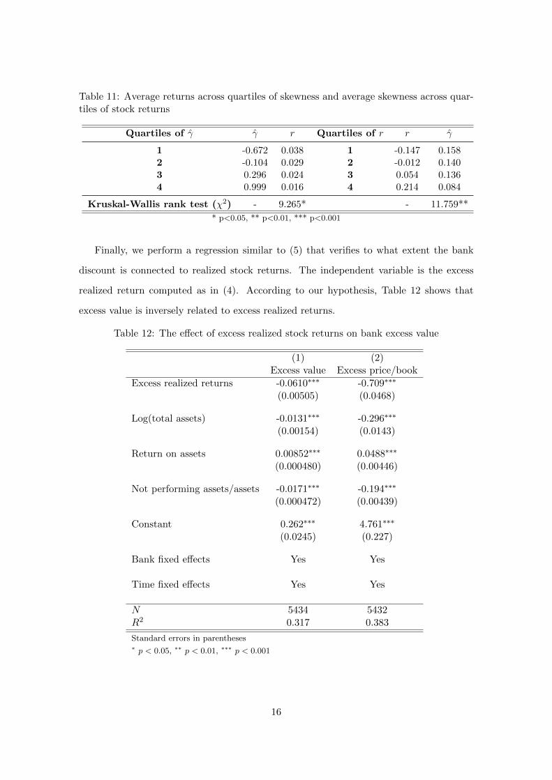
Table 11: Average returns across quartiles of skewness and average skewness across quar-tiles of stock returns
Quartiles of γ γ r Quartiles of r r γ
1 -0.672 0.038 1 -0.147 0.1582 -0.104 0.029 2 -0.012 0.1403 0.296 0.024 3 0.054 0.1364 0.999 0.016 4 0.214 0.084
Kruskal-Wallis rank test (χ2) - 9.265* - 11.759**
* p<0.05, ** p<0.01, *** p<0.001
Finally, we perform a regression similar to (5) that verifies to what extent the bank
discount is connected to realized stock returns. The independent variable is the excess
realized return computed as in (4). According to our hypothesis, Table 12 shows that
excess value is inversely related to excess realized returns.
Table 12: The effect of excess realized stock returns on bank excess value
(1) (2)Excess value Excess price/book
Excess realized returns -0.0610∗∗∗ -0.709∗∗∗
(0.00505) (0.0468)
Log(total assets) -0.0131∗∗∗ -0.296∗∗∗
(0.00154) (0.0143)
Return on assets 0.00852∗∗∗ 0.0488∗∗∗
(0.000480) (0.00446)
Not performing assets/assets -0.0171∗∗∗ -0.194∗∗∗
(0.000472) (0.00439)
Constant 0.262∗∗∗ 4.761∗∗∗
(0.0245) (0.227)
Bank fixed effects Yes Yes
Time fixed effects Yes Yes
N 5434 5432R2 0.317 0.383
Standard errors in parentheses∗ p < 0.05, ∗∗ p < 0.01, ∗∗∗ p < 0.001
16
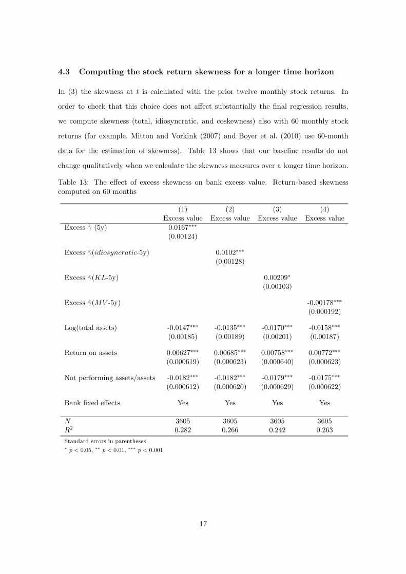
4.3 Computing the stock return skewness for a longer time horizon
In (3) the skewness at t is calculated with the prior twelve monthly stock returns. In
order to check that this choice does not affect substantially the final regression results,
we compute skewness (total, idiosyncratic, and coskewness) also with 60 monthly stock
returns (for example, Mitton and Vorkink (2007) and Boyer et al. (2010) use 60-month
data for the estimation of skewness). Table 13 shows that our baseline results do not
change qualitatively when we calculate the skewness measures over a longer time horizon.
Table 13: The effect of excess skewness on bank excess value. Return-based skewnesscomputed on 60 months
(1) (2) (3) (4)Excess value Excess value Excess value Excess value
Excess γ (5y) 0.0167∗∗∗
(0.00124)
Excess γ(idiosyncratic-5y) 0.0102∗∗∗
(0.00128)
Excess γ(KL-5y) 0.00209∗
(0.00103)
Excess γ(MV -5y) -0.00178∗∗∗
(0.000192)
Log(total assets) -0.0147∗∗∗ -0.0135∗∗∗ -0.0170∗∗∗ -0.0158∗∗∗
(0.00185) (0.00189) (0.00201) (0.00187)
Return on assets 0.00627∗∗∗ 0.00685∗∗∗ 0.00758∗∗∗ 0.00772∗∗∗
(0.000619) (0.000623) (0.000640) (0.000623)
Not performing assets/assets -0.0182∗∗∗ -0.0182∗∗∗ -0.0179∗∗∗ -0.0175∗∗∗
(0.000612) (0.000620) (0.000629) (0.000622)
Bank fixed effects Yes Yes Yes Yes
N 3605 3605 3605 3605R2 0.282 0.266 0.242 0.263
Standard errors in parentheses∗ p < 0.05, ∗∗ p < 0.01, ∗∗∗ p < 0.001
17

4.4 Asset pricing tests
The goal of this subsection is to verify the hypothesis that stock returns of diversified
banks incorporate a premium for negative skewness. To deal with this task we conduct a
number of asset-pricing tests.8 In the first place we analyze the pricing errors from different
models. More specifically, we compare a standard three-factor Fama-French model (see
Fama and French, 1993) to a model that includes a fourth factor for skewness (Harvey and
Siddique, 2000).9 The magnitude of the pricing error is assessed computing the F-statistic
of Gibbons et al. (1989). For this exercise we specify the following four-factor model for
the time series of returns exceeding the risk free rate rf :10
rj,t − rf = α+ β1rMKT,t + β2rSMB,t + β3rHML,t + β4γj,t + εt (9)
Table 14 reports the estimates from (9). We notice that excess returns are sensitive to the
market return, plus size and market-to-book factors. The negative sign on the regressor
measuring skewness suggests that the return premium is negative for stocks with positive
skewness. According to the test developed by Gibbons et al. (1989) the two models fit
the observed returns, since for both models we cannot reject the null hypothesis that the
pricing error is equal to zero. We obtain consistent results when we conduct the procedure
of Fama and MacBeth (1973) in Table 15. Fama and MacBeth (1973) develop a two-
step regression to test whether certain factors are able to describe stock returns, with the
ultimate goal to find the premium from exposure to these factors. The negative sign on
skewness that we observe in Table 15 indicates that a unit exposure to skewness over time
decreases the expected risk premium at the five percent level of significance.
8Amaya et al. (2015) compute realized moments for equity returns. They show that strategies basedon buying stocks in the lowest realized skewness decile while selling stocks in the highest realized skewnessdecile generates substantial returns.
9The details on how the Fama and French (1993) factors are calculated can be found at http://mba.
tuck.dartmouth.edu/pages/faculty/ken.french/Data_Library/f-f_factors.html.10F ∼ (N, T-N-1), where T is the number of observations and N is the number of explanatory variables.
18

Table 14: Regression models for bank return in excess to the risk-free rate
(1) (2)r − rf r − rf
rMKT 0.402∗∗∗ 0.405∗∗∗
(0.0299) (0.0299)
rSMB 0.149∗ 0.144∗
(0.0647) (0.0647)
rHML -0.522∗∗∗ -0.521∗∗∗
(0.0378) (0.0377)
γ -0.0123∗∗∗
(0.00298)
Constant 0.0155∗∗∗ 0.0170∗∗∗
(0.00208) (0.00211)
N 6130 6130R2 0.051 0.054F -test 60.065∗∗∗ 69.788∗∗∗
Standard errors in parentheses∗ p < 0.05, ∗∗ p < 0.01, ∗∗∗ p < 0.001
Table 15: Second step of the asset pricing test developed by Fama and MacBeth (1973)
(1) (2)r − rf r − rf
rMKT 0.00189∗ 0.00219∗
(0.000899) (0.000896)
rSMB 0.0101∗∗∗ 0.0106∗∗∗
(0.00102) (0.00104)
rHML 0.00207 0.000258(0.00275) (0.00282)
γ -0.0225∗
(0.00991)
Constant 0.0238∗∗∗ 0.0223∗∗∗
(0.00202) (0.00210)
N 147 147R2 0.425 0.445
Standard errors in parentheses∗ p < 0.05, ∗∗ p < 0.01, ∗∗∗ p < 0.001
19
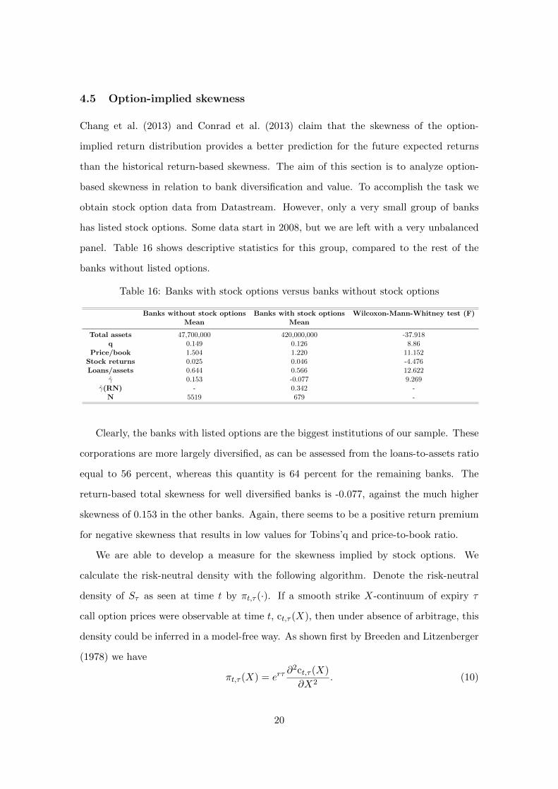
4.5 Option-implied skewness
Chang et al. (2013) and Conrad et al. (2013) claim that the skewness of the option-
implied return distribution provides a better prediction for the future expected returns
than the historical return-based skewness. The aim of this section is to analyze option-
based skewness in relation to bank diversification and value. To accomplish the task we
obtain stock option data from Datastream. However, only a very small group of banks
has listed stock options. Some data start in 2008, but we are left with a very unbalanced
panel. Table 16 shows descriptive statistics for this group, compared to the rest of the
banks without listed options.
Table 16: Banks with stock options versus banks without stock options
Banks without stock options Banks with stock options Wilcoxon-Mann-Whitney test (F)Mean Mean
Total assets 47,700,000 420,000,000 -37.918q 0.149 0.126 8.86
Price/book 1.504 1.220 11.152Stock returns 0.025 0.046 -4.476Loans/assets 0.644 0.566 12.622
γ 0.153 -0.077 9.269γ(RN) - 0.342 -
N 5519 679 -
Clearly, the banks with listed options are the biggest institutions of our sample. These
corporations are more largely diversified, as can be assessed from the loans-to-assets ratio
equal to 56 percent, whereas this quantity is 64 percent for the remaining banks. The
return-based total skewness for well diversified banks is -0.077, against the much higher
skewness of 0.153 in the other banks. Again, there seems to be a positive return premium
for negative skewness that results in low values for Tobins’q and price-to-book ratio.
We are able to develop a measure for the skewness implied by stock options. We
calculate the risk-neutral density with the following algorithm. Denote the risk-neutral
density of Sτ as seen at time t by πt,τ (·). If a smooth strike X-continuum of expiry τ
call option prices were observable at time t, ct,τ (X), then under absence of arbitrage, this
density could be inferred in a model-free way. As shown first by Breeden and Litzenberger
(1978) we have
πt,τ (X) = erτ∂2ct,τ (X)
∂X2. (10)
20

In reality, only a discrete set of strikes are available, which means that a considerable
amount of smoothing and curve fitting is needed before equation (10) can be used to
produce sensible numbers. Figlewski (2010, Section 2) provides a taxonomy of methods
that are used for this purpose. We prefer to use the non-parametric clamped spline
approach from Malz (2014), which is designed to avoid arbitrage opportunities that may
arise for other non-parametric approaches. In line with all other techniques, the procedure
requires data of reasonably good quality on the Black-Scholes implied volatility smile.
The volatility smile changes over time and with different tenors, resulting in the so-called
volatility surface σ(t,X, τ). The volatility surface translates into the market price of
European call options:
c(t,X, τ) = BS (St, X, τ, σ(t,X, τ), rt, qt) , (11)
with rt and qt the continuously compounded interest rate and cash dividend yield of the
underlying asset. We focus here on a single tenor τ , rather than the entire surface. The
technique can be summarized in three steps:
1. Interpolate and extrapolate the volatility smile using a cubic spline function that
is clumped at the endpoints. This corresponds to the assumption, that for very
deep out-of-the-money options the implied volatility is the same and equal to the
furthest strikes in the input data. Clamping the interpolated smile ensures the call
valuation function to be monotonic and convex in the exercise price, avoiding in this
way violations of no-arbitrage restrictions.
2. In order to calculate option prices, we use (11) by taking interpolated implied volatil-
ities as arguments.
3. Numerically difference the call valuation function with respect to the exercise price
in order to approximate the density function πt,τ (X). Therefore, the exercise-space
is discretized with a step size ∆:
πt,τ (X) ≈ ertτ 1
∆2[c (t,X + ∆, τ) + c (t,X −∆, τ)− 2c (t,X, τ)] . (12)
21
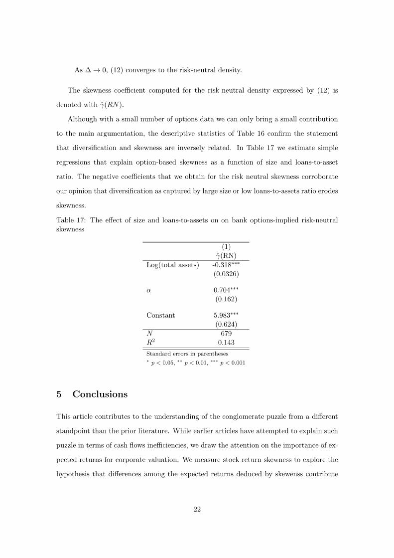
As ∆→ 0, (12) converges to the risk-neutral density.
The skewness coefficient computed for the risk-neutral density expressed by (12) is
denoted with γ(RN).
Although with a small number of options data we can only bring a small contribution
to the main argumentation, the descriptive statistics of Table 16 confirm the statement
that diversification and skewness are inversely related. In Table 17 we estimate simple
regressions that explain option-based skewness as a function of size and loans-to-asset
ratio. The negative coefficients that we obtain for the risk neutral skewness corroborate
our opinion that diversification as captured by large size or low loans-to-assets ratio erodes
skewness.
Table 17: The effect of size and loans-to-assets on on bank options-implied risk-neutralskewness
(1)γ(RN)
Log(total assets) -0.318∗∗∗
(0.0326)
α 0.704∗∗∗
(0.162)
Constant 5.983∗∗∗
(0.624)
N 679R2 0.143
Standard errors in parentheses∗ p < 0.05, ∗∗ p < 0.01, ∗∗∗ p < 0.001
5 Conclusions
This article contributes to the understanding of the conglomerate puzzle from a different
standpoint than the prior literature. While earlier articles have attempted to explain such
puzzle in terms of cash flows inefficiencies, we draw the attention on the importance of ex-
pected returns for corporate valuation. We measure stock return skewness to explore the
hypothesis that differences among the expected returns deduced by skewenss contribute
22
to determine the value discount of financial conglomerates in respect to comparable undi-
versified firms.
The empirical outcomes corroborate the argument that business diversification reduces
the upside potential of banks’ equity, i.e. it increases the likelihood to underperform. As
long as low skewness command high return premiums for the future, then the results lead
to the conclusion that investors demand high returns from diversified banks in order to
compensate the lack of good prospects. Thus, the financial conglomerate discount would
reflect equityholders’ expectations against the disruptive consequences for corporate value
that follow increasing business diversification.
Finally, by proposing to use skewness for the identification of future returns, we il-
lustrate that methodologies developed in the asset pricing research can be employed in
synergy with the corporate financial literature to address jointly the study of company
valuation.
23

References
Amaya, D., Christoffersen, P., Jacobs, K., and Vasquez, A. (2015). Does realized skewness
predict the cross-section of equity returns? Journal of Financial Economics, 118(1):135–
167.
Arditti, F. D. (1967). Risk and the required return on equity. The Journal of Finance,
22(1):19–36.
Baele, L., De Jonghe, O., and Vander Vennet, R. (2007). Does the stock market value
bank diversification? Journal of Banking and Finance, 31(7):1999–2023.
Bali, T. G., Hu, J., and Murray, S. (2017). Option implied volatility, skewness, and
kurtosis and the cross-section of expected stock returns. Georgetown McDonough School
of Business Research Paper.
Bali, T. G. and Murray, S. (2013). Does risk-neutral skewness predict the cross-section
of equity option portfolio returns? Journal of Financial and Quantitative Analysis,
48(4):1145–1171.
Barberis, N. and Huang, M. (2008). Stocks as lotteries: The implications of probability
weighting for security prices. American Economic Review, 98(5):2066–2100.
Berger, P. L. and Ofek, E. (1995). Diversifications effect on firm value. Journal of Financial
Economics, 37(1):39–65.
Bernardo, A. E., Chowdhry, B., and Goyal, A. (2007). Growth options, beta, and the cost
of capital. Financial Management, 36(2):1–13.
Boyer, B., Mitton, T., and Vorkink, K. (2010). Expected idiosyncratic skewness. Review
of Financial Studies, 23(1):170–202.
Breeden, D. T. and Litzenberger, R. (1978). Prices of state-contingent claims implicit in
option prices. Journal of Business, 51(4):621–651.
Brunnermeier, M. K., Gollier, C., and Parker, J. A. (2007). Optimal beliefs, asset prices,
and the preference for skewed returns. American Economic Review, 97(2):159–165.
24

Brunnermeier, M. K. and Parker, J. A. (2005). Optimal expectations. American Economic
Review, 95(4):1092–1118.
Campa, J. M. and Kedia, S. (2002). Explaining the diversification discount. The Journal
of Finance, 57(4):1731–1762.
Chang, B. Y., Christoffersen, P., and Jacobs, K. (2013). Market skewness risk and the
cross section of stock returns. Journal of Financial Economics, 107(1):46–68.
Conrad, J., Dittmar, R. F., and Ghysels, E. (2013). Ex Ante Skewness and Expected
Stock Returns. The Journal of Finance, 68(1):85–124.
Del Viva, L., Kasanen, E., and Trigeorgis, L. (2017). Real options, idiosyncratic skewness,
and diversification. Journal of Financial and Quantitative Analysis, 52(01):215–241.
Denis, D. J., Denis, D. K., and Sarin, A. (1997). Agency problems, equity ownership, and
corporate diversification. The Journal of Finance, 52(1):135–160.
Elsas, R., Hackethal, A., and Holzhauser, M. (2010). The anatomy of bank diversification.
Journal of Banking and Finance, 34(6):1274–1287.
Fama, E. F. and French, K. R. (1993). Common risk factors in the returns on stocks and
bonds. Journal of Financial Economics, 33(1):3–56.
Fama, E. F. and MacBeth, J. D. (1973). Risk, return, and equilibrium: Empirical tests.
Journal of Political Economy, 81(3):607–636.
Figlewski, S. (2010). Estimating the implied risk neutral density for the U.S. market
portfolio. In Volatility and Time Series Econometrics: Essays in Honor of Robert F.
Engle. Bollerslev, T., Russel, J., and Watson, M. Oxford University Press.
Gibbons, M. R., Ross, S. A., and Shanken, J. (1989). A test of the efficiency of a given
portfolio. Econometrica: Journal of the Econometric Society, pages 1121–1152.
Hadlock, C., Houston, J., and Ryngaert, M. (1999). The role of managerial incentives in
bank acquisitions. Journal of Banking & Finance, 23(2-4):221–249.
25

Harvey, C. R. and Siddique, A. (2000). Conditional skewness in asset pricing tests. The
Journal of Finance, 55(3):1263–1295.
Kraus, A. and Litzenberger, R. H. (1976). Skewness preference and the valuation of risk
assets. The Journal of Finance, 31(4):1085–1100.
Laeven, L. and Levine, R. (2007). Is there a diversification discount in financial conglom-
erates? Journal of Financial Economics, 85(2):331–367.
Lamont, O. A. and Polk, C. (2001). The diversification discount: Cash flows versus returns.
The Journal of Finance, 56(5):1693–1721.
Lang, L. H. P., Stulz, R. M., and Stulz, R. M. (1994). Tobin’s q, corporate diversification,
and firm performance. Source Journal of Political Economy, 102(6):1248–1280.
LeBaron, D. and Speidell, L. S. (1987). Why are the parts worth more than the sum¿‘chop
shop,” a corporate valuation model. In Conference Series Proceedings, volume 31, pages
78–101. Federal Reserve Bank of Boston.
Lins, K. and Servaes, H. (1999). International evidence on the value of corporate diversi-
fication. The Journal of Finance, 54(6):2215–2239.
Maksimovic, V. and Phillips, G. M. (2013). Conglomerate firms, internal capital markets,
and the theory of the firm. Annual Review of Financial Economics, 5(1):225–244.
Malz, A. M. (2014). A simple and reliable way to compute option-based risk-neutral
distributions. Federal Reserve Bank of New York Staff Report No. 677.
Mitton, T. and Vorkink, K. (2007). Equilibrium underdiversification and the preference
for skewness. Review of Financial Studies, 20(4):1255–1288.
Mitton, T. and Vorkink, K. (2010). Why do firms with diversification discounts have higher
expected returns? Journal of Financial and Quantitative Analysis, 45(06):1367–1390.
Ross, S. A., Westerfield, R. W., Jaffe, J. F., and Jordan, B. D. (2011). Core Principles
and Applications of Corporate Finance. McGraw-Hill/Irwin.
26

Saunders, A. and Walter, I. (2012). Financial architecture, systemic risk, and universal
banking. Financial Markets and Portfolio Management, 26(1):39–59.
Schmid, M. M. and Walter, I. (2009). Do financial conglomerates create or destroy eco-
nomic value? Journal of Financial Intermediation, 18(2):193–216.
Scott, R. C. and Horvath, P. A. (1980). On the direction of performance for moments of
higher order than the variance. The Journal of Finance, 35(4):915–919.
Stilger, P. S., Kostakis, A., and Poon, S.-H. (2016). What does risk-neutral skewness tell
us about future stock returns? Management Science, 63(6):1814–1834.
Stiroh, K. J. and Rumble, A. (2006). The dark side of diversification: The case of US
financial holding companies. Journal of Banking and Finance, 30(8):2131–2161.
Van Lelyveld, I. and Knot, K. (2009). Do financial conglomerates create or destroy value?
Evidence for the EU. Journal of Banking and Finance, 33(12):2312–2321.
Villalonga, B. (2004). Diversification discount or premium? New evidence from the busi-
ness information tracking series. The Journal of Finance, 59(2):479–506.
27