Statistics and Its Interface Volume 5 (2012) 221–236

Nonparametric estimation of the dependence of aspatial point process on spatial covariates

Adrian Baddeley∗, Ya-Mei Chang, Yong Song and Rolf Turner

In the statistical analysis of spatial point patterns, it isoften important to investigate whether the point patterndepends on spatial covariates. This paper describes non-parametric (kernel and local likelihood) methods for esti-mating the effect of spatial covariates on the point processintensity. Variance estimates and confidence intervals areprovided in the case of a Poisson point process. Techniquesare demonstrated with simulated examples and with appli-cations to exploration geology and forest ecology.

AMS 2000 subject classifications: Primary 62H11,62G07; secondary 62M30.Keywords and phrases: Confidence intervals, Densityestimation, Kernel smoothing, Local likelihood, Logistic re-gression, Point process intensity, Poisson point process, [Ge-ological] prospectivity mapping, Spatial covariates, Relativedistributions, Resource selection function, Weighted distri-bution.

1. INTRODUCTION

A common problem in the statistical analysis of spatialpoint patterns is to investigate the dependence of the pointpattern on spatial covariates. Applications include spatialepidemiology (e.g. disease risk as a function of environmen-tal exposure), spatial ecology (e.g. habitat preferences of or-ganisms), exploration geology (e.g. prospectivity of mineraldeposits predicted from survey data) and seismology.

Parametric models for this dependence, i.e. spatial pointprocess models which include an effect due to spatial co-variates, have been fitted to spatial point pattern data sincethe 1970’s [1, 7, 15, 19, 26, 29, 60]. Formal hypothesis testsfor the dependence of a point process on a spatial covariatefunction, under parametric assumptions, were developed in[11, 23, 48, 56, 66].

Nonparametric estimation of the effect of a spatial co-variate on a spatial point process has received less attentionuntil recently. An exception is the special case of spatial rela-tive risk or spatial residual risk where the covariates are theCartesian coordinates [12, 13, 25, 38, 43, 44] and/or the timecoordinate [28, 57]. Nonparametric estimation is importanthere because simple parametric models are inappropriate,and the sample size is large.

∗Corresponding author.

In this paper we consider spatial point process modelsthat depend on one or more spatial covariates with continu-ous numerical values. We assume the point process intensityis a function of the covariates, and study nonparametric esti-mators of this function. Our estimators are rescaled versionsof several existing kernel estimators for a probability densityfrom biased sample data [30, 42] and their analogues usinglocal likelihood density estimation [39, 49, 50]. Related ker-nel estimators were proposed in [33, 34].

Suppose the dataset is a finite set y of points in somed-dimensional space representing the locations and/or oc-currence times of events. Additionally we have the valuesX(u) of a spatial covariate (real- or vector-valued) at everyspatial location u. We model y as a realisation of a spatialpoint process Y (often, but not necessarily, assumed to be aPoisson process) with intensity function λ(u) depending onX(u),

(1) λ(u) = ρ(X(u))

where ρ is a function to be determined. This paper proposesnonparametric estimators of ρ.

In ecological applications where the points are the loca-tions of individual organisms, ρ is a resource selection func-tion [53] reflecting preference for particular environmentalconditions x. In geological applications where the points arethe locations of valuable mineral deposits, ρ is an index ofthe prospectivity [14] or predicted frequency of undiscovereddeposits as a function of geological and geochemical covari-ates x.

The simplest and most popular parametric model for de-pendence of Y on X is the loglinear model

(2) λ(u) = exp(β�X(u))

where β is a parameter vector. In applied literature thereappears to be frequent confusion between the parametricloglinear model (2) and the nonparametric general relation-ship (1).

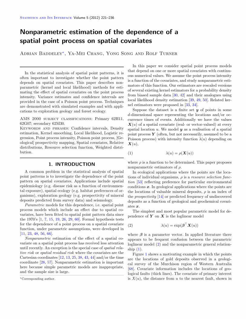
Figure 1 shows a motivating example in which the pointsare the locations of gold deposits observed in a geologi-cal survey of the Murchison region of Western Australia[68]. Covariate information includes the locations of geo-logical faults (thick lines). The covariate of primary interestis X(u), the distance from u to the nearest fault, shown in

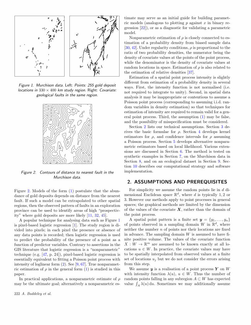
Figure 1. Murchison data. Left: Points: 255 gold depositlocations in 330× 400 km study region. Right: Covariate:

geological faults in the same region.

Figure 2. Contours of distance to nearest fault in theMurchison data.

Figure 2. Models of the form (1) postulate that the abun-dance of gold deposits depends on distance from the nearestfault. If such a model can be extrapolated to other spatialregions, then the observed pattern of faults in an explorationprovince can be used to identify areas of high “prospectiv-ity” where gold deposits are more likely [11, 32, 45].

A popular technique for analysing data such as Figure 1is pixel-based logistic regression [1]. The study region is di-vided into pixels; in each pixel the presence or absence ofany data points is recorded; then logistic regression is usedto predict the probability of the presence of a point as afunction of predictor variables. Contrary to assertions in theGIS literature that logistic regression is a “nonparametric”technique (e.g. [47, p. 24]), pixel-based logistic regression isessentially equivalent to fitting a Poisson point process withintensity of loglinear form (2). See [9, 67]. True nonparamet-ric estimation of ρ in the general form (1) is studied in thispaper.

In practical applications, a nonparametric estimate of ρmay be the ultimate goal; alternatively a nonparametric es-

timate may serve as an initial guide for building paramet-ric models (analogous to plotting p against x in binary re-gression [22]), or as a diagnostic for validating a parametricmodel.

Nonparametric estimation of ρ is closely connected to es-timation of a probability density from biased sample data[30, 42]. Under regularity conditions, ρ is proportional to theratio of two probability densities, the numerator being thedensity of covariate values at the points of the point process,while the denominator is the density of covariate values atrandom locations in space. Estimation of ρ is also related tothe estimation of relative densities [37].

Estimation of a spatial point process intensity is slightlydifferent from estimation of a probability density in severalways. First, the intensity function is not normalised (i.e.not required to integrate to unity). Second, in spatial dataanalysis it may be inappropriate or contentious to assume aPoisson point process (corresponding to assuming i.i.d. ran-dom variables in density estimation) so that techniques forestimation of intensity are required to remain valid for a gen-eral point process. Third, the assumption (1) may be false,and the possibility of misspecification must be considered.

Section 2 lists our technical assumptions. Section 3 de-rives the basic formulae for ρ. Section 4 develops kernelestimators for ρ, and confidence intervals for ρ assuminga Poisson process. Section 5 develops alternative nonpara-metric estimators based on local likelihood. Various exten-sions are discussed in Section 6. The method is tested onsynthetic examples in Section 7, on the Murchison data inSection 8, and on an ecological dataset in Section 9. Sec-tion 10 describes our computational strategy and softwareimplementation.

2. ASSUMPTIONS AND PREREQUISITES

For simplicity we assume the random points lie in d di-mensional Euclidean space R

d, where d is typically 1, 2 or3. However our methods apply to point processes in generalspaces; the graphical methods are limited by the dimensionof the values of the covariate X, rather than the domain ofthe point process.

A spatial point pattern is a finite set y = {y1, . . . , yn}of points observed in a sampling domain W in R

d, whereneither the number n of points nor their locations are fixedin advance. The sampling domain W is assumed to have fi-nite positive volume. The values of the covariate functionX : W → R

m are assumed to be known exactly at all lo-cations u ∈ W . In practice, the covariate values may haveto be spatially interpolated from observed values at a finiteset of locations uj but we do not consider the errors arisingfrom this step.

We assume y is a realisation of a point process Y on Wwith intensity function λ(u), u ∈ W . Thus the number ofrandom points falling in any subregion A ⊂ W has expectedvalue

∫Aλ(u) du. Sometimes we may additionally assume

222 A. Baddeley et al.

Y is a Poisson process. Processes with a singular intensitymeasure, such as earthquake epicentres concentrated alonga geological fault, can be dealt with using a singular baselinemeasure as explained in Section 6.1.

Throughout the paper we use the following two facts.Suppose Y is any point process inW with intensity functionλ(u), and h : W → R is a real function. Then we haveCampbell’s formula

(3) E

[∑i

h(yi)

]=

∫W

h(u)λ(u) du

provided∫W

|h(u)|λ(u) du < ∞. Additionally if Y is a Pois-son process,

(4) var[∑i

h(yi)] =

∫W

h(u)2λ(u) du

provided the right-hand side is finite [24, p. 188].

3. THEORY FOR A REAL COVARIATE

In this section we consider a single, real-valued covariatefunction X on W , i.e. a function X : W → R. Let

(5) G(x) =1

|W |

∫W

1{X(u) ≤ x} du

be the spatial cumulative distribution function of X, where|W | denotes the d-dimensional volume of the window W .Equivalently G(x) = P{X(U) ≤ x} is the c.d.f. of the valueX(U) at a uniformly distributed random point U in W .Assume G has derivative g; a sufficient condition is that Xbe differentiable with nonzero gradient (see Appendix A.1).It will be convenient to consider the unnormalised versionsG∗(x) = |W |G(x) and g∗(x) = |W |g(x).

We assume G∗ is known exactly, or to a very high accu-racy. This is true when X is a spatial coordinate, or whenX values are known on a very fine pixel grid, and G∗ is wellapproximated numerically.

Suppose Y is a point process inW with intensity functionof the form (1) for some function ρ. Then [24, p. 22], [59, p.17] the values xi = X(yi) constitute a point process on R

with intensity function

(6) f∗(x) = ρ(x)g∗(x), x ∈ R.

This is the pivotal relationship between the observations xi

and the target function ρ. The expected number of pointsin Y is

μ =

∫W

λ(u) du =

∫W

ρ(X(u)) du =

∫ ∞

−∞ρ(x)g∗(x) dx.

Conditional on the number n of data points, the valuesx1, . . . , xn are exchangeable, with marginal probability den-sity f(x) = f∗(x)/μ. If Y is a Poisson process on W , then

the values xi constitute a Poisson process on R, and areconditionally i.i.d. random variables given n. Hence

(7) ρ(x) =f∗(x)

g∗(x)= κ

f(x)

g(x)

where κ = μ/|W | is the average intensity. Apart from a scalefactor, ρ is a relative probability density for the distributionof the values xi = X(yi) relative to the distribution thatwould be obtained if the process Y had constant intensityon W . For practical interpretation of results, it is importantthat the values of ρ(x) are intensities, expressed in unitswith dimension length−d.

If (1) does not hold, the formulae in this section remaintrue when ρ(x) is replaced by ρ(x), a weighted average valueof λ(u) over the contour {u ∈ W : X(u) = x}. See Ap-pendix A.2. This issue of misspecification does not arise fordensity estimation in one-dimensional space.

4. KERNEL ESTIMATORS OF ρ

Kernel smoothing is the simplest nonparametric methodin this context, with advantages that include theoreticaltractability, superior computational speed and reliability,and disadvantages including bias. In large datasets, rapidcomputation is important and the bias of the kernel estima-tor is tolerable for appropriate choices of bandwidth. Kernelestimation of the intensity of a Poisson process is discussedin [46, section 6.2, pp 236–250] including the optimal rateof convergence.

Equation (6) shows that estimation of ρ is closely relatedto estimating a probability density from a biased sample.Jones [42] described two kernel estimators for this problem,and El Barmi and Simonoff [30] a third kernel estimatorbased on the probability integral transformation.

In our context the analogues of Jones’ estimators of ρfrom the observed values xi = X(yi) are the “ratio” form

(8) ρR(x) =1

g∗(x)

∑i

k(xi − x)

and the “reweighted” form

(9) ρW(x) =∑i

1

g∗(xi)k(xi − x)

while the analogue of El Barmi and Simonoff’s “transforma-tion” estimator is

(10) ρT(x) =1

|W |∑i

k(G(xi)−G(x)).

Here k is a smoothing kernel on the real line, and again Gis the spatial c.d.f. (5).

Guan [33] proposed a kernel estimator that is similar tothe ratio form (8). It is discussed below.

Nonparametric estimation of the dependence of a spatial point process on spatial covariates 223

The rationale for the ratio form (8) is the plug-in principleapplied to (7), since

(11) ρR(x) =f∗(x)

g∗(x)= κ

f(x)

g(x)

where κ = n/|W | is the usual unbiased estimator of κ (andthe MLE if Y is Poisson),

(12) f(x) =1

n

∑i

k(xi − x)

is the usual fixed-bandwidth kernel estimator of the density

f , and f∗(x) = nf(x) is the corresponding unnormalisedkernel estimator of f∗(x). The rationale for the reweightedform (9) is that the random measure with masses 1/g∗(xi) atthe points xi has intensity ρ(x), by an application of (3). Thetransformation estimator (10) is justified by the fact thatthe values ti = G(xi) have intensity q(t) = |W | ρ(G−1(t))on [0, 1] (see Appendix A.4).

In the context of density estimation, Jones [42] showedthat neither the ratio nor the reweighting estimator is uni-formly optimal, but that the reweighting estimator has bet-ter performance overall. A similar statement is likely to holdin this context. The transformation estimator ρT is a simple,fast and appropriate form of variable-bandwidth smoothinginsofar as it depends on the covariate values but is otherwisenot adaptive to features of the point process. It is likely toimprove the accuracy of ρ(x) for values x where data arescarce, and may also improve bandwidth selection. The es-timator ρT could also be edge-corrected at the endpoints 0and 1 using standard techniques.

Computational implementation and performance are dis-cussed in Section 10.

Assuming (1) holds, the expectation of ρR(x) is, by (3),

E[ρR(x)] =1

g∗(x)

∫W

k(X(u)− x)λ(u) du(13)

=

∫ ∞

−∞k(x′ − x)ρ(x′)

g∗(x′)

g∗(x)dx′

where the last expression is obtained by a change of vari-ables from u to x′ = X(u). Similarly the reweighting andtransformation estimators have expectation

E[ρW(x)] =

∫ ∞

−∞k(x′ − x)ρ(x′) dx′(14)

E[ρT(x)] =

∫ 1

0

k(t−G(x))ρ(G−1(t)) dt.(15)

The kernel estimators are biased, as usual (e.g. [17]) withbias controlled by the kernel bandwidth and the regularityof ρ and g∗ (with the exception that the regularity of g∗

does not affect the bias of ρW). A proof for ρR is given inAppendix A.3.

Guan [33] proposed a kernel estimator that is similarto the ratio form (8) except that g∗(x) is replaced by∫W

k(X(u)−x) du, a kernel smoothed counterpart of g∗(x),using the same kernel k for the numerator f∗(x) and denom-inator g∗(x). However, the numerator and denominator arebased on datasets of different sizes, and this strategy willtypically lead to over-smoothing of the denominator g∗(x).Calculations similar to those in Appendix A.3 show thatGuan’s estimator typically has greater bias than ρR(x).

Bandwidth selection can be performed using existingmethods for bandwidth selection in density estimation, be-cause of the close connection between the two problems.Silverman’s rule of thumb using the fifth root of the numberof points [64, eq. (3.31), p. 48] performed well in our exam-ples. Cross-validation methods [61, 63] tended to produceunacceptably small bandwidths.

To construct approximate confidence intervals, we assumeadditionally that Y is a Poisson process. Since the values xi

constitute a Poisson process with intensity f∗, the varianceof ρR(x) for fixed x is, by (4),

var[ρR(x)] = g∗(x)−2

∫W

k(x−X(u))2λ(u) du(16)

= g∗(x)−2

∫ ∞

−∞k(x− x′)2ρ(x′)g∗(x′) dx′

Similarly

var[ρW(x)] =

∫ ∞

−∞k(x− x′)2

ρ(x′)

g∗(x′)dx′(17)

var[ρT(x)] =1

|W |

∫ 1

0

k(t−G(x))2ρ(G−1(t)) dt.(18)

In particular if k is the Gaussian kernel k(v) = kσ(v) =(σ√2π)−1 exp(−v2/(2σ2)) then kσ(v)

2 = αkτ (v) where τ =σ/

√2 and α = 1/(2σ

√π) = 1/(2τ

√2π), so that pointwise

unbiased estimators of the variances (16)–(18) are, by (3),

vR(x) = αg∗(x)−2∑i

kτ (xi − x)(19)

vW (x) = α∑i

kτ (xi − x)

g∗(xi)2(20)

vT (x) = α|W |−2∑i

kτ (ti −G(x))(21)

where again xi = X(yi) and ti = G(xi). This calculationassumes g∗ (or equivalently G) is fixed and known.

For small bandwidths the variances of the three kernelestimators behave as

(22) var[ρ(x)] ∼ ρ(x)

g∗(x)

as intuitively expected: g∗(x) plays the role of the “samplesize” for estimation of ρ(x) at small bandwidths. Estimator

224 A. Baddeley et al.

variance var[ρ(x)] decreases with sample size g∗(x), but in-creases with intensity ρ(x), due to the variance propertiesof the Poisson process.

The kernel estimators (8)–(10) of ρ(x) are asymptoticallynormal under large-sample conditions, e.g. [46, p. 240]. How-ever, confidence intervals for ρ(x) with good small-sampleproperties are difficult to construct, because the natural esti-mators of variance (19)–(21) have strong positive correlationwith the estimators ρ(x) themselves. This parallels the well-known difficulty in constructing confidence intervals for aprobability density based on kernel estimates [16, 35, 36, 40].

In density estimation, the theoretically optimal band-width for constructing confidence intervals is typicallysmaller than the optimal bandwidth for point estimation.However, this insight did not deliver any practical bene-fit in our experiments, because confidence bands obtainedusing smaller bandwidths were typically too irregular. Ac-cordingly we propose constructing confidence intervals in thenaive form ρ(x)± z

√v(x) from the estimators (8)–(10) and

variance estimators (19)–(21), where z is the 100(1−α/2)%critical value of the standard normal distribution.

The assumption of a Poisson point process is not essen-tial. For a general point process, the variance of the ker-nel estimators can be expressed in terms of the intensityand pair correlation function of the point process, using thesecond order Campbell formula, e.g. [6, 33]. If the pointprocess is regular (negatively associated) then the Poissonassumption leads to overestimates of the variance of ρ, andconservative confidence intervals. Concern arises when thepoint process is believed to be clustered (positively associ-ated) so that the variance is underestimated by (19)–(21).In this case, a more accurate variance estimate could be ob-tained by estimating the pair correlation function, providedwe are willing to impose additional model assumptions, suchas second-order reweighted stationarity [5] or a Cox processmodel [54]. However, explicit model assumptions do not sitwell with the nonparametric approach, and may be diffi-cult to verify, especially in the case of clustered patterns[10]. Alternatively, bootstrap confidence intervals might beobtained by spatial resampling [52]. Further discussion isbeyond the scope of the present paper.

5. ALTERNATIVE NONPARAMETRICESTIMATORS

Alternatives to kernel estimation of ρ include splinesmoothing, locally weighted regression [18] and local like-lihood density estimation [39, 49, 50].

The appropriate counterparts of the kernel estimators(8)–(10) can be determined by expressing these estimatorsas multiples of the fixed-bandwidth kernel density estimatorf(x) = (1/n)

∑i k(xi −x), and then replacing f by another

nonparametric density estimator.Let f(x | x1, . . . , xn) denote a nonparametric estimator

of the probability density based on observations xi, and

f(x | x1, . . . , xn;w1, . . . , wn) the corresponding estimatorwhen observations xi have prior weights wi. Then the coun-terparts of the estimators (8)–(10) are

ρR(x) =κ

g(x)f(x | x1, . . . , xn)(23)

ρW(x) = (∑i

wi) f(x | x1, . . . , xn; w1, . . . , wn)(24)

ρT(x) = κ f(G(x) | G(x1), . . . , G(xn))(25)

where wi = 1/g∗(xi) and κ = n/|W |.The variance of the estimators (23)–(25) depends on

the choice of nonparametric density estimator f . Here weconsider the case of local likelihood density estimation[39, 49, 50] and assume Y is a Poisson process.

The local likelihood density estimator f is asymptoticallynormal in large samples. A normal approximation to log f ismore accurate and more natural. Estimators of the varianceof log f are implemented in open-source software such as thelocfit package [51].

Noting that all the estimators ρ are of the form ρ(x) =

Mf(x), we have

var log ρ(x) = var logM+var log f(x)+2cov(logM, log f(x)).

Using the delta method we may approximate var logM ≈(varM)/(EM)2 and

cov(logM, log f(x)) ≈ cov(M, f(x))

EM Ef≈ E(ρ(x)− ρ(x))

ρ(x),

the relative bias of ρ(x), essentially equivalent to the relative

bias of f(x). Estimates of this quantity are available fromthe local likelihood procedure.

For the ratio form (23) the scale factor is M = κ/g(x) =n/g∗(x) so that var logM = var logN ≈ E(N)/(E(N))2 =1/E(N).

For the reweighting estimator (24) we have M =∑i 1/g

∗(xi) so that

EM =

∫W

1

g∗(X(u))λ(u)du

=

∫1

g∗(x)ρ(x)g∗(x)dx =

∫ρ(x)dx

and

varM =

∫W

1

g∗(X(u))2λ(u)du

=

∫1

g∗(x)2ρ(x)g∗(x)dx =

∫ρ(x)

g∗(x)dx.

For the transformation estimator (25) we have M = κ soagain var logM = var logN ≈ E(N)/(E(N))2 = 1/E(N).

These calculations yield approximations to the varianceof log ρ(x), which can be used to construct asymptotically

Nonparametric estimation of the dependence of a spatial point process on spatial covariates 225

valid confidence intervals for ρ(x) based on the asymptoticnormal distribution for log ρ(x). The finite-sample prop-erties of these confidence intervals are likely to be bet-ter than those of the confidence intervals for kernel es-timates described in the previous section, because of theabovementioned problems with variance estimation for ker-nel smoothers.

6. EXTENSIONS

6.1 Relative risk model

Still assuming a real-valued covariateX, consider the gen-eralization of (1) to

(26) λ(u) = ρ(X(u))B(u)

where B(u) is a fixed and known function, serving as a base-line. For example, in applications to spatial epidemiology,B(u) could be the spatially-varying density of the underly-ing population of susceptible individuals, and ρ(X(u)) therelative risk of the events represented by the point process,expressed as a probability or rate relative to the susceptiblepopulation, and depending on an explanatory “risk factor”X [26, 27]. Alternatively B(u) may be an artificial baselinewhich serves to stabilise estimator variability. The theory ofSection 3 can be adapted to this model, yielding the basicidentity

(27) ρ(x) =f∗(x)

g∗B(x)= κB

f(x)

gB(x)

where g∗B is the derivative of the B-weighted spatial c.d.f.of X

(28) G∗B(x) =

∫W

1{X(u) ≤ x}B(u) du

and κB = μ/∫W

B(u) du is the usual unbiased estimator(and MLE in the Poisson case) of the constant κ in theconstant relative risk model λ(u) = κB(u).

The estimators proposed in Sections 4 and 5 can be ap-plied simply by replacing g, g∗, G,G∗ by their B-weightedcounterparts gB , g

∗B , GB , G

∗B respectively. Properties of ρ

described in Sections 4 and 5 and Appendix A.3 also ap-ply mutatis mutandis. Thus, for example, the B-weightedanalogue of (8) is

(29) ρR,B(x) =1

g∗B(x)

∑i

k(xi − x).

The practical interpretation of the relative risk (or “residualrisk”) term ρ(x) in this Section is slightly different from thatof the absolute intensity ρ(x) in previous Sections. Typicallythe baseline function B(u) is a valid intensity function. Inthat case, the relative risk ρ(x) is dimensionless, and the

constant value ρ(x) ≡ 1 corresponds to the baseline or nullmodel λ(u) = B(u).

In many applications, the baseline B(u) would also beestimated from data. Variance estimation and interval esti-mation of ρ(x) then depend on the distribution of the esti-mator B(u) and on the joint distribution of the observationsxi with B(·). Examples of this analysis arise in case-controlstudies in spatial epidemiology [38, 43, 44].

Alternatively the baseline intensity function B(u) maybe replaced by a baseline intensity measure. Then (28) isreplaced by an integral with respect to the baseline measure,and similarly for gB , g

∗B , GB . This accommodates situations

where the point process intensity is singular, for example,where points are concentrated on a curve.

6.2 Vector covariate

Now consider an m-dimensional vector-valued covariatefunction X(u) = (X1(u), . . . , Xm(u)). Multivariate densityestimation from weighted samples was discussed in [2].

The approach described above can be applied providedthe spatial distribution of X is absolutely continuous onR

m. The counterpart of G∗ is the unnormalised joint c.d.f.

G∗(x1, . . . , xm) =

∫W

1{X1(u) ≤ x1, . . . , Xm(u) ≤ xm} du.

The ratio estimator (8) and reweighting estimator (9), andtheir counterparts (23)–(24) for relative/residual risk (Sec-tion 6.1), can be applied directly to anm-dimensional vectorcovariate function X using an m-dimensional kernel k. Thevariance formulae (16)–(17) generalise immediately by re-placing one-dimensional bym-dimensional integration, sincethey are derived from (4).

Absolute continuity of the distribution of X implies, inparticular, that the image X(W ) = {X(u) : u ∈ W}must not be contained in any lower-dimensional subset ofR

m. This excludes algebraically dependent covariates suchas polynomials (i.e. where Xi(u) = Z(u)i is the ith term ina polynomial in a real-valued covariate Z).

Polynomials are a special case of the separable model

(30) λ(u) = ρ1(X1(u)) . . . ρm(Xm(u))A(u)

where ρj are functions to be estimated, and A(u) is a knownfunction serving as a baseline. When attention is focusedon one of the functions ρj , holding others fixed, (30) col-lapses to a model of the form (26). The technique of sec-tion 6.1 applies, and ρj can be estimated by the analogue of(29). The appropriate variance calculations depend on themethod used to estimate the reference function B.

If covariates are high-dimensional and if prior informationis lacking, it becomes important to reduce dimensionality.Dimension reduction techniques for spatial point processeswere proposed in [34].

226 A. Baddeley et al.

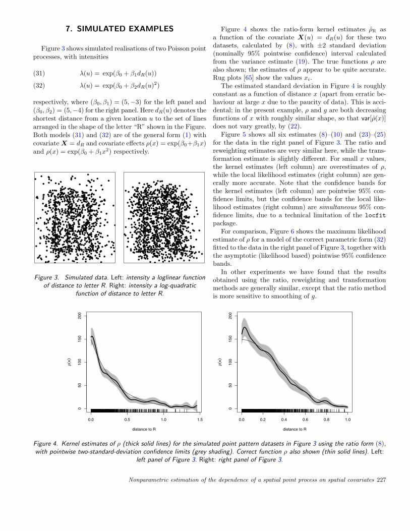
7. SIMULATED EXAMPLES

Figure 3 shows simulated realisations of two Poisson pointprocesses, with intensities

λ(u) = exp(β0 + β1dR(u))(31)

λ(u) = exp(β0 + β2dR(u)2)(32)

respectively, where (β0, β1) = (5,−3) for the left panel and(β0, β2) = (5,−4) for the right panel. Here dR(u) denotes theshortest distance from a given location u to the set of linesarranged in the shape of the letter “R” shown in the Figure.Both models (31) and (32) are of the general form (1) withcovariate X = dR and covariate effects ρ(x) = exp(β0+β1x)and ρ(x) = exp(β0 + β1x

2) respectively.

Figure 3. Simulated data. Left: intensity a loglinear functionof distance to letter R. Right: intensity a log-quadratic

function of distance to letter R.

Figure 4 shows the ratio-form kernel estimates ρR asa function of the covariate X(u) = dR(u) for these twodatasets, calculated by (8), with ±2 standard deviation(nominally 95% pointwise confidence) interval calculatedfrom the variance estimate (19). The true functions ρ arealso shown; the estimates of ρ appear to be quite accurate.Rug plots [65] show the values xi.

The estimated standard deviation in Figure 4 is roughlyconstant as a function of distance x (apart from erratic be-haviour at large x due to the paucity of data). This is acci-dental; in the present example, ρ and g are both decreasingfunctions of x with roughly similar shape, so that var[ρ(x)]does not vary greatly, by (22).

Figure 5 shows all six estimates (8)–(10) and (23)–(25)for the data in the right panel of Figure 3. The ratio andreweighting estimates are very similar here, while the trans-formation estimate is slightly different. For small x values,the kernel estimates (left column) are overestimates of ρ,while the local likelihood estimates (right column) are gen-erally more accurate. Note that the confidence bands forthe kernel estimates (left column) are pointwise 95% con-fidence limits, but the confidence bands for the local like-lihood estimates (right column) are simultaneous 95% con-fidence limits, due to a technical limitation of the locfit

package.For comparison, Figure 6 shows the maximum likelihood

estimate of ρ for a model of the correct parametric form (32)fitted to the data in the right panel of Figure 3, together withthe asymptotic (likelihood based) pointwise 95% confidencebands.

In other experiments we have found that the resultsobtained using the ratio, reweighting and transformationmethods are generally similar, except that the ratio methodis more sensitive to smoothing of g.

Figure 4. Kernel estimates of ρ (thick solid lines) for the simulated point pattern datasets in Figure 3 using the ratio form (8),with pointwise two-standard-deviation confidence limits (grey shading). Correct function ρ also shown (thin solid lines). Left:

left panel of Figure 3. Right: right panel of Figure 3.

Nonparametric estimation of the dependence of a spatial point process on spatial covariates 227

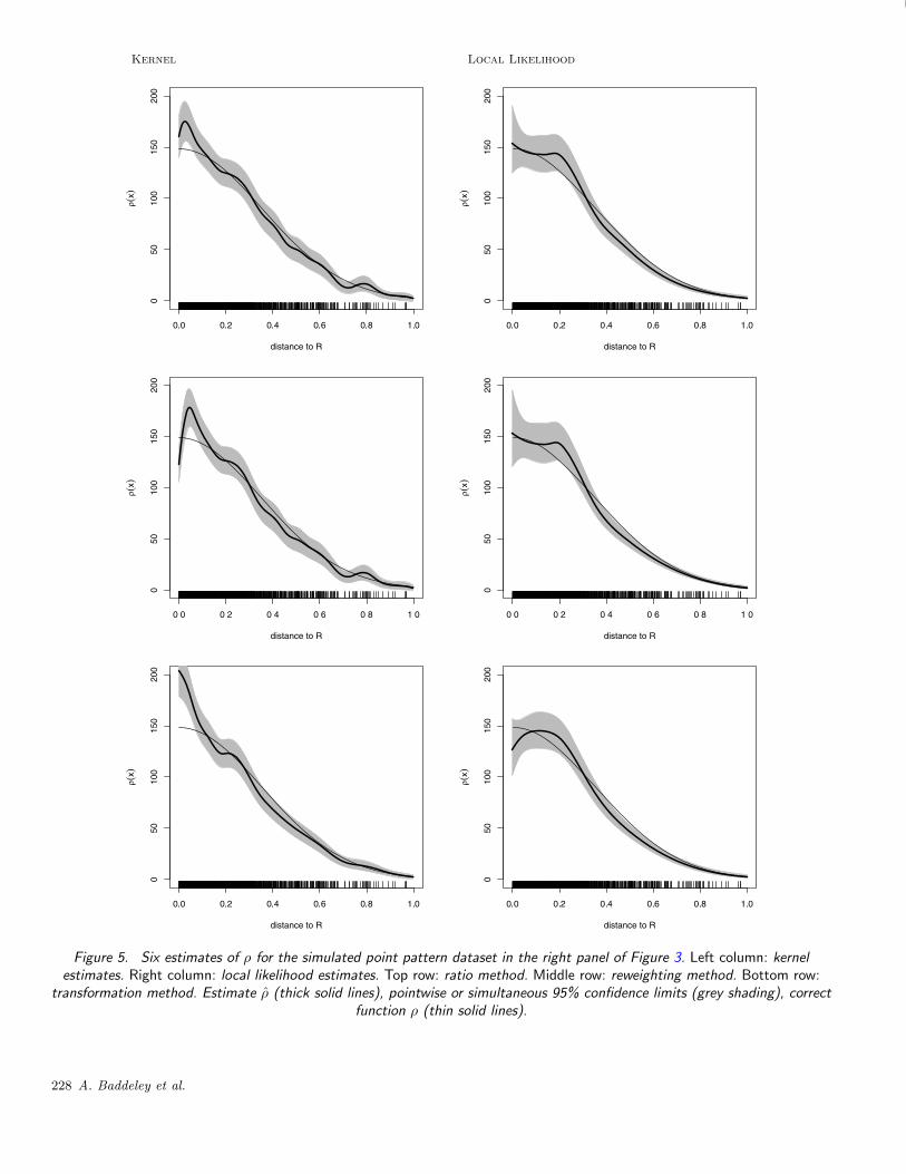
Figure 5. Six estimates of ρ for the simulated point pattern dataset in the right panel of Figure 3. Left column: kernelestimates. Right column: local likelihood estimates. Top row: ratio method. Middle row: reweighting method. Bottom row:

transformation method. Estimate ρ (thick solid lines), pointwise or simultaneous 95% confidence limits (grey shading), correctfunction ρ (thin solid lines).

228 A. Baddeley et al.

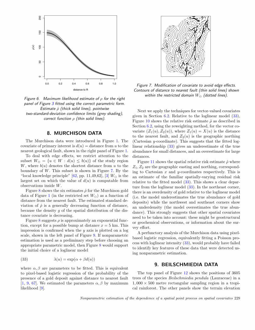
Figure 6. Maximum likelihood estimate of ρ for the rightpanel of Figure 3 fitted using the correct parametric form.

Estimate ρ (thick solid lines), pointwisetwo-standard-deviation confidence limits (grey shading),

correct function ρ (thin solid lines).

8. MURCHISON DATA

The Murchison data were introduced in Figure 1. Thecovariate of primary interest is d(u) = distance from u to thenearest geological fault, shown in the right panel of Figure 1.

To deal with edge effects, we restrict attention to thesubset W� = {u ∈ W : d(u) ≤ b(u)} of the study regionW , where b(u) denotes the shortest distance from u to theboundary of W . This subset is shown in Figure 7. By the“local knowledge principle” [62, pp. 11,49,62], [3] W� is thelargest set on which the value of d(u) is computable fromobservations inside W .

Figure 8 shows the six estimates ρ for the Murchison golddata of Figure 1 (in the restricted set W�) as a function ofdistance from the nearest fault. The estimated standard de-viation of ρ is a generally decreasing function of distance,because the density g of the spatial distribution of the dis-tance covariate is decreasing.

Figure 8 suggests ρ is approximately an exponential func-tion, except for a possible bump at distance x = 5 km. Thisimpression is confirmed when the y axis is plotted on a logscale, shown in the left panel of Figure 9. If nonparametricestimation is used as a preliminary step before choosing anappropriate parametric model, then Figure 8 would supportthe initial choice of a loglinear model

(33) λ(u) = exp(α+ βd(u))

where α, β are parameters to be fitted. This is equivalentto pixel-based logistic regression of the probability of thepresence of a gold deposit against distance to nearest fault[1, 9, 67]. We estimated the parameters α, β by maximumlikelihood [9].

Figure 7. Modification of covariate to avoid edge effects.Contours of distance to nearest fault (thin solid lines) shown

within the restricted domain W� (dotted lines).

Next we apply the techniques for vector-valued covariatesgiven in Section 6.2. Relative to the loglinear model (33),Figure 10 shows the relative risk estimate ρ as described inSection 6.2, using the reweighting method, for the vector co-variate (Z1(u), Z2(u)), where Z1(u) = X(u) is the distanceto the nearest fault, and Z2(u) is the geographic northing(Cartesian y-coordinate). This suggests that the fitted log-linear relationship (33) gives an underestimate of the trueabundance for small distances, and an overestimate for largedistances.

Figure 11 shows the spatial relative risk estimate ρ whereZ1, Z2 are the geographic easting and northing, correspond-ing to Cartesian x and y-coordinates respectively. This isan estimate of the familiar spatially-varying residual riskrelative to the fitted model (33). This shows a clear depar-ture from the loglinear model (33). In the northeast corner,there is an overdensity of gold relative to the loglinear model(i.e. the model underestimates the true abundance of golddeposits) while the northwest and southeast corners showan underdensity (the model overestimates the true abun-dance). This strongly suggests that other spatial covariatesneed to be taken into account: these might be geostructuralor geochemical observations, or information about the sur-vey effort.

A perfunctory analysis of the Murchison data using pixel-based logistic regression, equivalently fitting a Poisson pro-cess with loglinear intensity (33), would probably have failedto identify key features of these data that were detected us-ing nonparametric estimation.

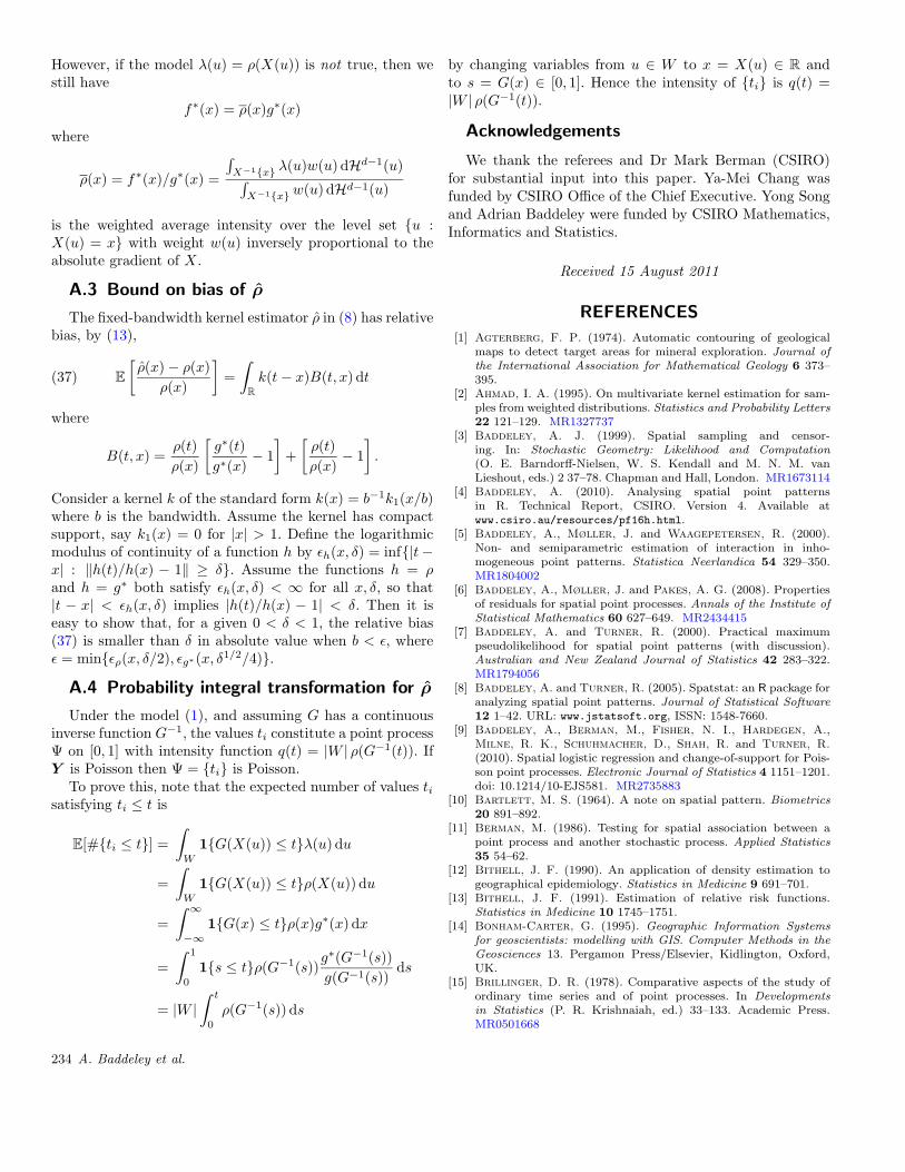
9. BEILSCHMIEDIA DATA

The top panel of Figure 12 shows the positions of 3605trees of the species Beilschmiedia pendula (Lauraceae) in a1, 000 × 500 metre rectangular sampling region in a tropi-cal rainforest. The other panels show the terrain elevation

Nonparametric estimation of the dependence of a spatial point process on spatial covariates 229

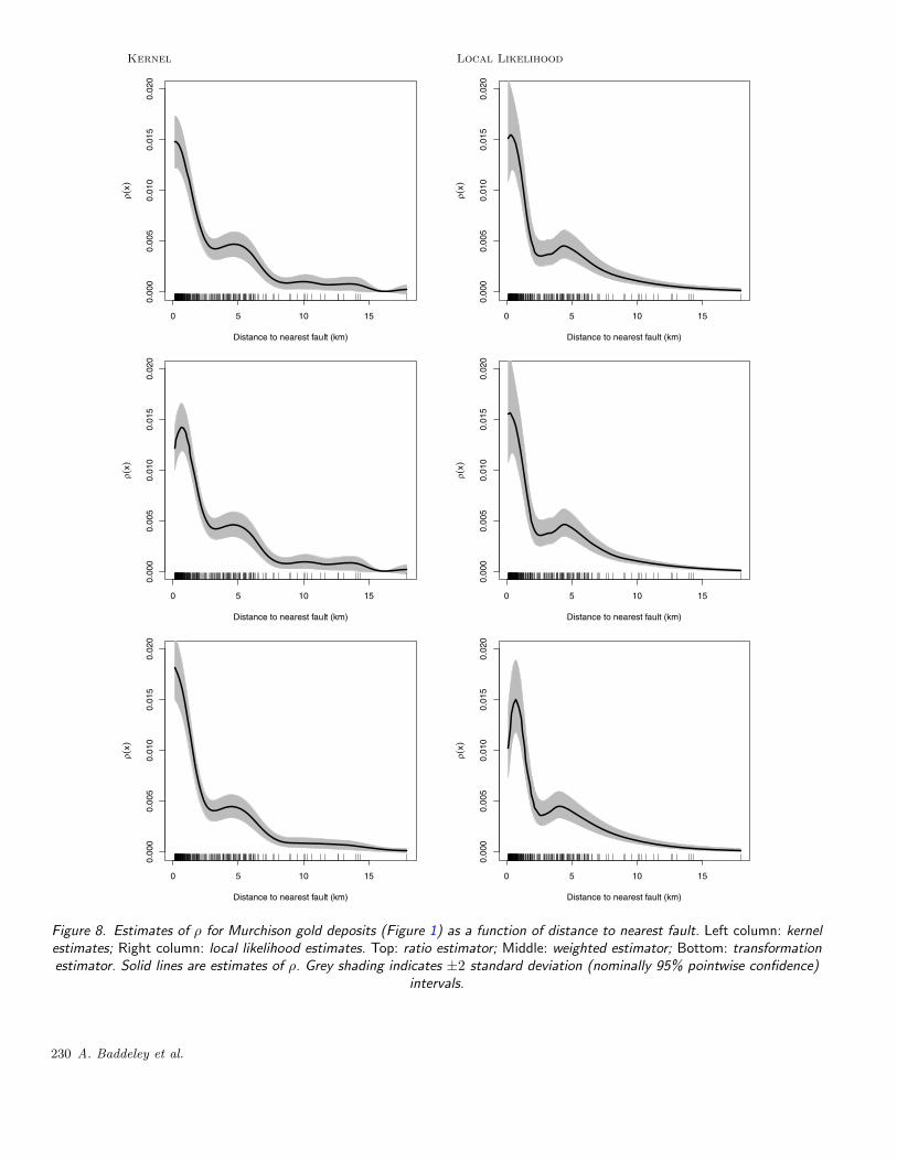
Figure 8. Estimates of ρ for Murchison gold deposits (Figure 1) as a function of distance to nearest fault. Left column: kernelestimates; Right column: local likelihood estimates. Top: ratio estimator; Middle: weighted estimator; Bottom: transformationestimator. Solid lines are estimates of ρ. Grey shading indicates ±2 standard deviation (nominally 95% pointwise confidence)

intervals.

230 A. Baddeley et al.

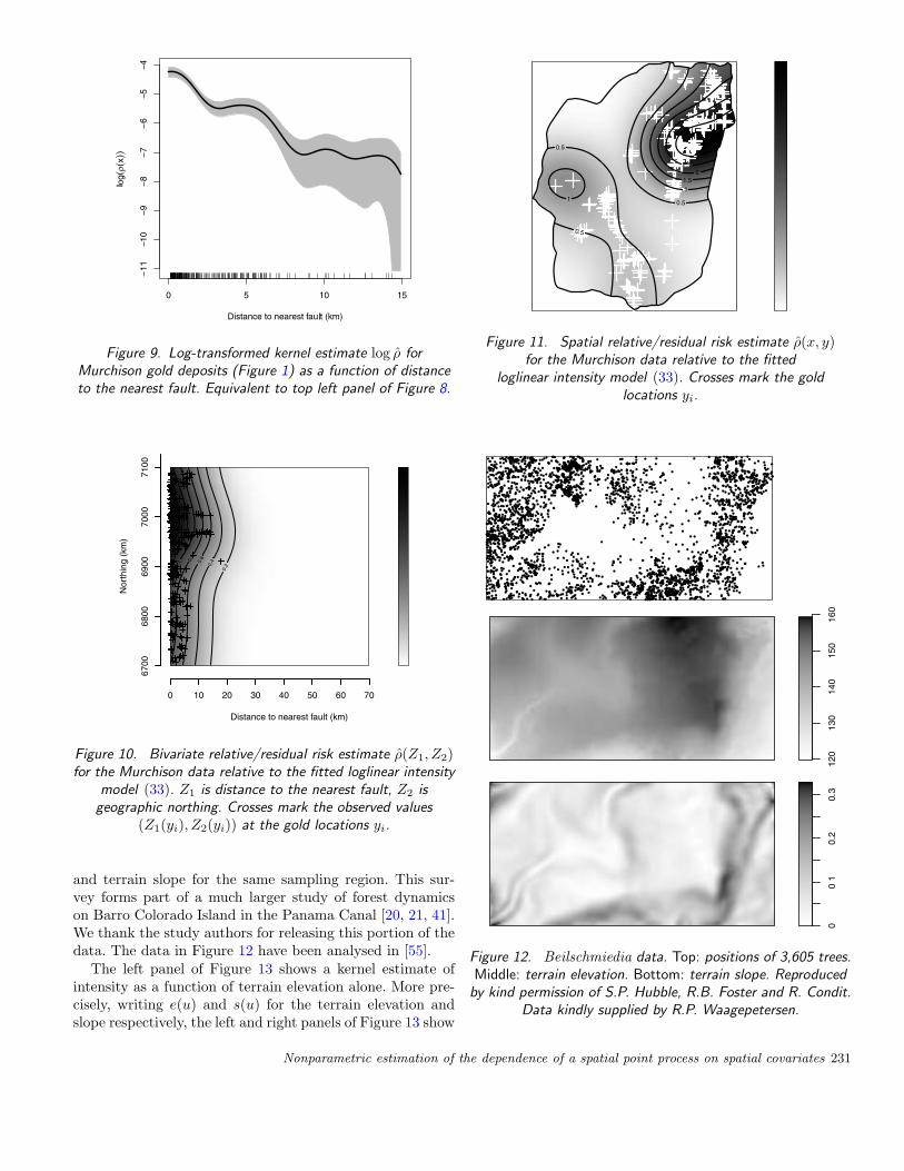
Figure 9. Log-transformed kernel estimate log ρ forMurchison gold deposits (Figure 1) as a function of distanceto the nearest fault. Equivalent to top left panel of Figure 8.

Figure 10. Bivariate relative/residual risk estimate ρ(Z1, Z2)for the Murchison data relative to the fitted loglinear intensity

model (33). Z1 is distance to the nearest fault, Z2 isgeographic northing. Crosses mark the observed values

(Z1(yi), Z2(yi)) at the gold locations yi.

and terrain slope for the same sampling region. This sur-vey forms part of a much larger study of forest dynamicson Barro Colorado Island in the Panama Canal [20, 21, 41].We thank the study authors for releasing this portion of thedata. The data in Figure 12 have been analysed in [55].

The left panel of Figure 13 shows a kernel estimate ofintensity as a function of terrain elevation alone. More pre-cisely, writing e(u) and s(u) for the terrain elevation andslope respectively, the left and right panels of Figure 13 show

Figure 11. Spatial relative/residual risk estimate ρ(x, y)for the Murchison data relative to the fitted

loglinear intensity model (33). Crosses mark the goldlocations yi.

Figure 12. Beilschmiedia data. Top: positions of 3,605 trees.Middle: terrain elevation. Bottom: terrain slope. Reproducedby kind permission of S.P. Hubble, R.B. Foster and R. Condit.

Data kindly supplied by R.P. Waagepetersen.

Nonparametric estimation of the dependence of a spatial point process on spatial covariates 231

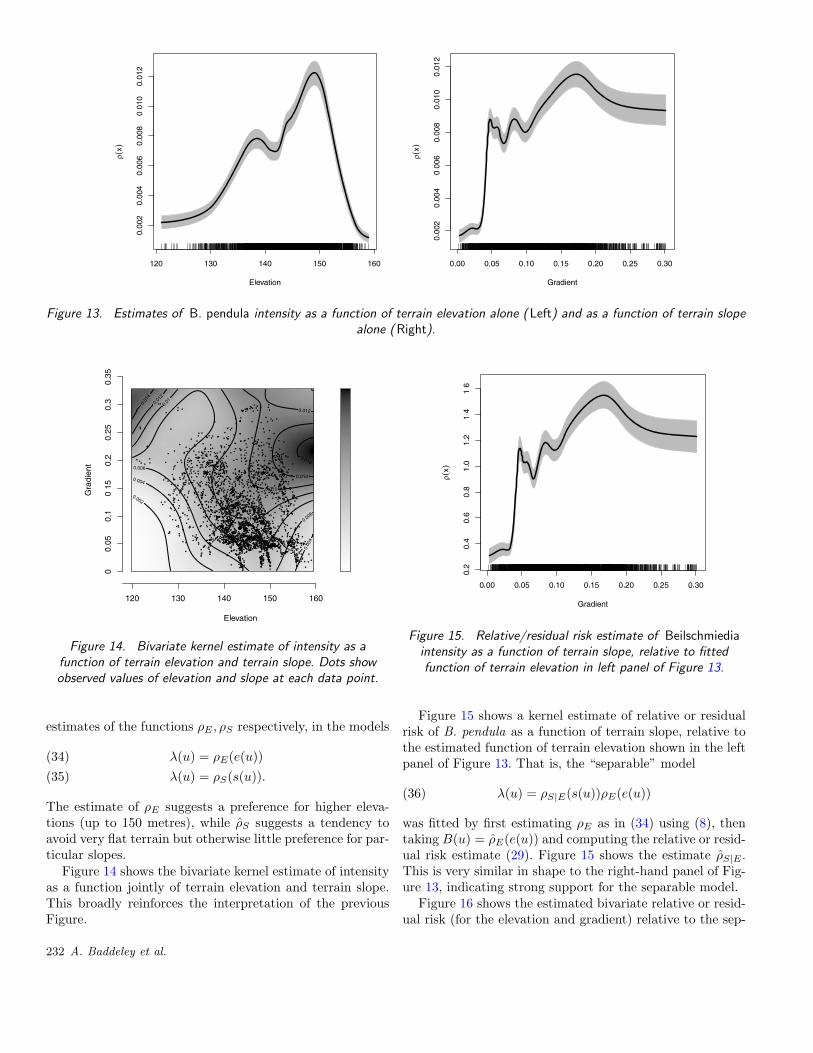
Figure 13. Estimates of B. pendula intensity as a function of terrain elevation alone (Left) and as a function of terrain slopealone (Right).

Figure 14. Bivariate kernel estimate of intensity as afunction of terrain elevation and terrain slope. Dots showobserved values of elevation and slope at each data point.

estimates of the functions ρE , ρS respectively, in the models

λ(u) = ρE(e(u))(34)

λ(u) = ρS(s(u)).(35)

The estimate of ρE suggests a preference for higher eleva-tions (up to 150 metres), while ρS suggests a tendency toavoid very flat terrain but otherwise little preference for par-ticular slopes.

Figure 14 shows the bivariate kernel estimate of intensityas a function jointly of terrain elevation and terrain slope.This broadly reinforces the interpretation of the previousFigure.

Figure 15. Relative/residual risk estimate of Beilschmiediaintensity as a function of terrain slope, relative to fittedfunction of terrain elevation in left panel of Figure 13.

Figure 15 shows a kernel estimate of relative or residualrisk of B. pendula as a function of terrain slope, relative tothe estimated function of terrain elevation shown in the leftpanel of Figure 13. That is, the “separable” model

(36) λ(u) = ρS|E(s(u))ρE(e(u))

was fitted by first estimating ρE as in (34) using (8), thentaking B(u) = ρE(e(u)) and computing the relative or resid-ual risk estimate (29). Figure 15 shows the estimate ρS|E .This is very similar in shape to the right-hand panel of Fig-ure 13, indicating strong support for the separable model.

Figure 16 shows the estimated bivariate relative or resid-ual risk (for the elevation and gradient) relative to the sep-

232 A. Baddeley et al.

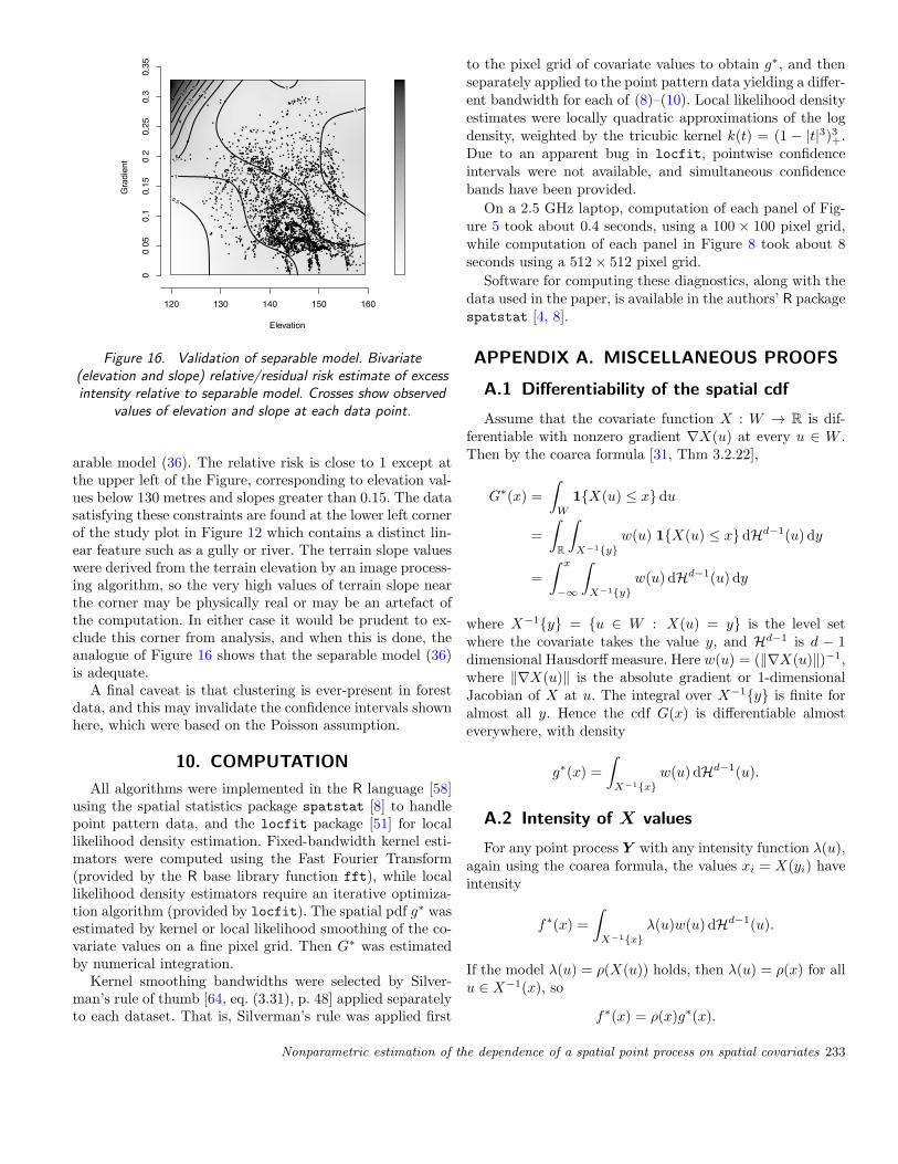
Figure 16. Validation of separable model. Bivariate(elevation and slope) relative/residual risk estimate of excessintensity relative to separable model. Crosses show observed

values of elevation and slope at each data point.

arable model (36). The relative risk is close to 1 except atthe upper left of the Figure, corresponding to elevation val-ues below 130 metres and slopes greater than 0.15. The datasatisfying these constraints are found at the lower left cornerof the study plot in Figure 12 which contains a distinct lin-ear feature such as a gully or river. The terrain slope valueswere derived from the terrain elevation by an image process-ing algorithm, so the very high values of terrain slope nearthe corner may be physically real or may be an artefact ofthe computation. In either case it would be prudent to ex-clude this corner from analysis, and when this is done, theanalogue of Figure 16 shows that the separable model (36)is adequate.

A final caveat is that clustering is ever-present in forestdata, and this may invalidate the confidence intervals shownhere, which were based on the Poisson assumption.

10. COMPUTATION

All algorithms were implemented in the R language [58]using the spatial statistics package spatstat [8] to handlepoint pattern data, and the locfit package [51] for locallikelihood density estimation. Fixed-bandwidth kernel esti-mators were computed using the Fast Fourier Transform(provided by the R base library function fft), while locallikelihood density estimators require an iterative optimiza-tion algorithm (provided by locfit). The spatial pdf g∗ wasestimated by kernel or local likelihood smoothing of the co-variate values on a fine pixel grid. Then G∗ was estimatedby numerical integration.

Kernel smoothing bandwidths were selected by Silver-man’s rule of thumb [64, eq. (3.31), p. 48] applied separatelyto each dataset. That is, Silverman’s rule was applied first

to the pixel grid of covariate values to obtain g∗, and thenseparately applied to the point pattern data yielding a differ-ent bandwidth for each of (8)–(10). Local likelihood densityestimates were locally quadratic approximations of the logdensity, weighted by the tricubic kernel k(t) = (1 − |t|3)3+.Due to an apparent bug in locfit, pointwise confidenceintervals were not available, and simultaneous confidencebands have been provided.

On a 2.5 GHz laptop, computation of each panel of Fig-ure 5 took about 0.4 seconds, using a 100 × 100 pixel grid,while computation of each panel in Figure 8 took about 8seconds using a 512× 512 pixel grid.

Software for computing these diagnostics, along with thedata used in the paper, is available in the authors’ R packagespatstat [4, 8].

APPENDIX A. MISCELLANEOUS PROOFS

A.1 Differentiability of the spatial cdf

Assume that the covariate function X : W → R is dif-ferentiable with nonzero gradient ∇X(u) at every u ∈ W .Then by the coarea formula [31, Thm 3.2.22],

G∗(x) =

∫W

1{X(u) ≤ x} du

=

∫R

∫X−1{y}

w(u) 1{X(u) ≤ x} dHd−1(u) dy

=

∫ x

−∞

∫X−1{y}

w(u) dHd−1(u) dy

where X−1{y} = {u ∈ W : X(u) = y} is the level setwhere the covariate takes the value y, and Hd−1 is d − 1dimensional Hausdorff measure. Here w(u) = (‖∇X(u)‖)−1,where ‖∇X(u)‖ is the absolute gradient or 1-dimensionalJacobian of X at u. The integral over X−1{y} is finite foralmost all y. Hence the cdf G(x) is differentiable almosteverywhere, with density

g∗(x) =

∫X−1{x}

w(u) dHd−1(u).

A.2 Intensity of X values

For any point process Y with any intensity function λ(u),again using the coarea formula, the values xi = X(yi) haveintensity

f∗(x) =

∫X−1{x}

λ(u)w(u) dHd−1(u).

If the model λ(u) = ρ(X(u)) holds, then λ(u) = ρ(x) for allu ∈ X−1(x), so

f∗(x) = ρ(x)g∗(x).

Nonparametric estimation of the dependence of a spatial point process on spatial covariates 233

However, if the model λ(u) = ρ(X(u)) is not true, then westill have

f∗(x) = ρ(x)g∗(x)

where

ρ(x) = f∗(x)/g∗(x) =

∫X−1{x} λ(u)w(u) dHd−1(u)∫

X−1{x} w(u) dHd−1(u)

is the weighted average intensity over the level set {u :X(u) = x} with weight w(u) inversely proportional to theabsolute gradient of X.

A.3 Bound on bias of ρ

The fixed-bandwidth kernel estimator ρ in (8) has relativebias, by (13),

(37) E

[ρ(x)− ρ(x)

ρ(x)

]=

∫R

k(t− x)B(t, x) dt

where

B(t, x) =ρ(t)

ρ(x)

[g∗(t)

g∗(x)− 1

]+

[ρ(t)

ρ(x)− 1

].

Consider a kernel k of the standard form k(x) = b−1k1(x/b)where b is the bandwidth. Assume the kernel has compactsupport, say k1(x) = 0 for |x| > 1. Define the logarithmicmodulus of continuity of a function h by εh(x, δ) = inf{|t−x| : ‖h(t)/h(x) − 1‖ ≥ δ}. Assume the functions h = ρand h = g∗ both satisfy εh(x, δ) < ∞ for all x, δ, so that|t − x| < εh(x, δ) implies |h(t)/h(x) − 1| < δ. Then it iseasy to show that, for a given 0 < δ < 1, the relative bias(37) is smaller than δ in absolute value when b < ε, whereε = min{ερ(x, δ/2), εg∗(x, δ1/2/4)}.

A.4 Probability integral transformation for ρ

Under the model (1), and assuming G has a continuousinverse function G−1, the values ti constitute a point processΨ on [0, 1] with intensity function q(t) = |W | ρ(G−1(t)). IfY is Poisson then Ψ = {ti} is Poisson.

To prove this, note that the expected number of values tisatisfying ti ≤ t is

E[#{ti ≤ t}] =∫W

1{G(X(u)) ≤ t}λ(u) du

=

∫W

1{G(X(u)) ≤ t}ρ(X(u)) du

=

∫ ∞

−∞1{G(x) ≤ t}ρ(x)g∗(x) dx

=

∫ 1

0

1{s ≤ t}ρ(G−1(s))g∗(G−1(s))

g(G−1(s))ds

= |W |∫ t

0

ρ(G−1(s)) ds

by changing variables from u ∈ W to x = X(u) ∈ R andto s = G(x) ∈ [0, 1]. Hence the intensity of {ti} is q(t) =|W | ρ(G−1(t)).

Acknowledgements

We thank the referees and Dr Mark Berman (CSIRO)for substantial input into this paper. Ya-Mei Chang wasfunded by CSIRO Office of the Chief Executive. Yong Songand Adrian Baddeley were funded by CSIRO Mathematics,Informatics and Statistics.

Received 15 August 2011

REFERENCES

[1] Agterberg, F. P. (1974). Automatic contouring of geologicalmaps to detect target areas for mineral exploration. Journal ofthe International Association for Mathematical Geology 6 373–395.

[2] Ahmad, I. A. (1995). On multivariate kernel estimation for sam-ples from weighted distributions. Statistics and Probability Letters22 121–129. MR1327737

[3] Baddeley, A. J. (1999). Spatial sampling and censor-ing. In: Stochastic Geometry: Likelihood and Computation(O. E. Barndorff-Nielsen, W. S. Kendall and M. N. M. vanLieshout, eds.) 2 37–78. Chapman and Hall, London. MR1673114

[4] Baddeley, A. (2010). Analysing spatial point patternsin R. Technical Report, CSIRO. Version 4. Available atwww.csiro.au/resources/pf16h.html.

[5] Baddeley, A., Møller, J. and Waagepetersen, R. (2000).Non- and semiparametric estimation of interaction in inho-mogeneous point patterns. Statistica Neerlandica 54 329–350.MR1804002

[6] Baddeley, A., Møller, J. and Pakes, A. G. (2008). Propertiesof residuals for spatial point processes. Annals of the Institute ofStatistical Mathematics 60 627–649. MR2434415

[7] Baddeley, A. and Turner, R. (2000). Practical maximumpseudolikelihood for spatial point patterns (with discussion).Australian and New Zealand Journal of Statistics 42 283–322.MR1794056

[8] Baddeley, A. and Turner, R. (2005). Spatstat: an R package foranalyzing spatial point patterns. Journal of Statistical Software12 1–42. URL: www.jstatsoft.org, ISSN: 1548-7660.

[9] Baddeley, A., Berman, M., Fisher, N. I., Hardegen, A.,Milne, R. K., Schuhmacher, D., Shah, R. and Turner, R.

(2010). Spatial logistic regression and change-of-support for Pois-son point processes. Electronic Journal of Statistics 4 1151–1201.doi: 10.1214/10-EJS581. MR2735883

[10] Bartlett, M. S. (1964). A note on spatial pattern. Biometrics20 891–892.

[11] Berman, M. (1986). Testing for spatial association between apoint process and another stochastic process. Applied Statistics35 54–62.

[12] Bithell, J. F. (1990). An application of density estimation togeographical epidemiology. Statistics in Medicine 9 691–701.

[13] Bithell, J. F. (1991). Estimation of relative risk functions.Statistics in Medicine 10 1745–1751.

[14] Bonham-Carter, G. (1995). Geographic Information Systemsfor geoscientists: modelling with GIS. Computer Methods in theGeosciences 13. Pergamon Press/Elsevier, Kidlington, Oxford,UK.

[15] Brillinger, D. R. (1978). Comparative aspects of the study ofordinary time series and of point processes. In Developmentsin Statistics (P. R. Krishnaiah, ed.) 33–133. Academic Press.MR0501668

234 A. Baddeley et al.

[16] Chen, S. X. (1996). Empirical likelihood confidence intervalsfor nonparametric density estimation. Biometrika 83 329–341.MR1439787

[17] Chu, C. K. and Marron, J. S. (1991). Choosing a kernel regres-sion estimator. Statistical Science 6 404-436. MR1146907

[18] Cleveland, W. S. (1979). Robust locally weighted regression andsmoothing scatterplots. Journal of the American Statistical As-sociation 74 829–836. MR0556476

[19] Clyde, M. and Strauss, D. (1991). Logistic regression for spatialpair-potential models. In Spatial Statistics and Imaging, (A. Pos-solo, ed.). Lecture Notes – Monograph Series 20 II 14–30. Insti-tute of Mathematical Statistics ISBN 0-940600-27-7. MR1195558

[20] Condit, R. (1998). Tropical Forest Census Plots. Springer Verlag.[21] Condit, R., Hubbell, S. P. and Foster, R. B. (1996). Changes

in tree species abundance in a neotropical forest: impact ofclimate change. Journal of Tropical Ecology 12 231–256.

[22] Copas, J. B. (1983). Plotting p against x. Applied Statistics 3225–31. MR0713965

[23] Cox, D. R. (1972). The statistical analysis of dependencies inpoint processes. In Stochastic Point Processes (P. A. W. Lewis,ed.) 55–66. Wiley, New York. MR0375705

[24] Daley, D. J. and Vere-Jones, D. (1988). An Introductionto the Theory of Point Processes. Springer Verlag, New York.MR0950166

[25] Diggle, P. J. (1985). A kernel method for smoothing pointprocess data. Journal of the Royal Statistical Society, Series C(Applied Statistics) 34 138–147.

[26] Diggle, P. J. (1990). A point process modelling approachto raised incidence of a rare phenomenon in the vicinity of aprespecified point. Journal of the Royal Statistical Society, SeriesA 153 349–362.

[27] Diggle, P. J. and Rowlingson, B. (1994). A conditionalapproach to point process modelling of elevated risk. Journal ofthe Royal Statistical Society, Series A (Statistics in Society) 157433–440.

[28] Diggle, P. J., Rowlingson, B. and Su, T. L. (2005). Point pro-cess methodology for on-line spatio-temporal disease surveillance.Environmetrics 16 423–434. MR2147534

[29] Diggle, P., Morris, S., Elliott, P. and Shaddick, G. (1997).Regression modelling of disease risk in relation to point sources.Journal of the Royal Statistical Society, Series A 160 491–505.

[30] El Barmi, H. and Simonoff, J. S. (2000). Transformationbased density estimation for weighted distributions. Journal ofNonparametric Statistics 12 861–878. MR1802580

[31] Federer, H. (1969). Geometric Measure Theory. SpringerVerlag, Heidelberg. MR0257325

[32] Groves, D. I., Goldfarb, R. J., Knox-Robinson, C. M.,Ojala, J., Gardoll, S., Yun, G. Y. and Holyland, P. (2000).Late-kinematic timing of orogenic gold deposits and significancefor computer-based exploration techniques with emphasis on theYilgarn Block, Western Australia. Ore Geology Reviews 17 1–38.

[33] Guan, Y. (2008). On consistent nonparametric intensity estima-tion for inhomogeneous spatial point processes. Journal of theAmerican Statistical Association 103 1238–1247. MR2528839

[34] Guan, Y. and Wang, H. (2010). Sufficient dimension reductionfor spatial point processes directed by Gaussian random fields.Journal of the Royal Statistical Society, Series B 72 367–387.MR2758117

[35] Hall, P. (1992). The effect of bias estimation on coverageaccuracy of bootstrap confidence intervals for a probabilitydensity. Annals of Statistics 20 675–694. MR1165587

[36] Hall, P. (2002). The bootstrap and Edgeworth expansion.Springer.

[37] Handcock, M. S. and Morris, M. (1999). Relative DistributionMethods in the Social Sciences. Springer-Verlag, New York.MR2000e:91112 MR1705294

[38] Hazelton, M. L. and Davies, T. M. (2009). Inference basedon kernel estimates of the relative risk function in geographicalepidemiology. Biometrical Journal 51 98–109. MR2667514

[39] Hjort, N. L. and Jones, M. C. (1996). Locally parametricdensity estimation. Ann. Statist. 24 1619–1649. MR1416653

[40] Horowitz, J. L. (2001). The bootstrap. In Handbook of Econo-metrics, (J. J. Heckman and E. Leamer, eds.) 5 3159–3228.North-Holland, Amsterdam.

[41] Hubbell, S. P. and Foster, R. B. (1983). Diversity of canopytrees in a neotropical forest and implications for conservation. InTropical Rain Forest: Ecology and Management (S. L. Sutton,T. C. Whitmore and A. C. Chadwick, eds.) 25–41. BlackwellScientific Publications, Oxford.

[42] Jones, M. C. (1991). Kernel density estimation for length-biaseddata. Biometrika 78 511–519. MR1130919

[43] Kelsall, J. E. and Diggle, P. J. (1995a). Kernel estimation ofrelative risk. Bernoulli 1 3–16. MR1354453

[44] Kelsall, J. E. and Diggle, P. J. (1995b). Non-parametricestimation of spatial variation in relative risk. Statistics inMedicine 14 2335–2342.

[45] Knox-Robinson, C. M. and Groves, D. I. (1997). Gold prospec-tivity mapping using a geographic information system (GIS),with examples from the Yilgarn Block of Western Australia.Chronique de la Recherche Miniere 529 127–138.

[46] Kutoyants, Y. A. (1998). Statistical Inference for SpatialPoisson Processes. Lecture Notes in Statistics 134. Springer,New York. MR1644620

[47] Kvamme, K. L. (2006). There and back again: revisiting arche-ological locational modeling. In GIS and Archaeological SiteModelling (M. W. Mehrer and K. L. Wescott, eds.) 3–40.CRC Press.

[48] Lawson, A. B. (1993). On the analysis of mortality eventsaround a prespecified fixed point. Journal of the Royal StatisticalSociety, Series A 156 363–377.

[49] Loader, C. (1996). Local likelihood and density estimation.Ann. Statist. 24 1602–1618. MR1416652

[50] Loader, C. (1999). Local Regression and Likelihood. Springer,New York. MR1704236

[51] Loader, C. (2010). locfit: Local Regression, Likelihood andDensity Estimation. R package version 1.5-6.

[52] Loh, J. M. (2008). A fast and valid spatial bootstrap forcorrelation functions. Astrophysical Journal 681 726–734.

[53] Manly, B. J. F., McDonald, L. L. and Thomas, D. L. (1993).Resource Selection by Animals: Statistical Design and Analysisfor Field Studies. Chapman and Hall, London.

[54] Møller, J. and Waagepetersen, R. P. (2004). StatisticalInference and Simulation for Spatial Point Processes. Chapmanand Hall/CRC, Boca Raton. MR2004226

[55] Møller, J. and Waagepetersen, R. P. (2007). Modern spa-tial point process modelling and inference (with discussion).Scandinavian Journal of Statistics 34 643–711. MR2396935

[56] Morton-Jones, A. J., Diggle, P. J. and Elliott, P. (1999).Investigation of excess environmental risk around putativesources: Stone’s test with covariate adjustment. Statistics inMedicine 18 189–197.

[57] Ogata, Y. (2001). Increased probability of large earthquakesnear aftershock regions with relative quiescence. Journal ofGeophysical Research 106 8729–8744. MR1915525

[58] R Development Core Team, (2009). R: A language and en-vironment for statistical computing R Foundation for StatisticalComputing, Vienna, Austria ISBN 3-900051-07-0.

[59] Reiss, R. D. (1993). A Course on Point Processes. Springer.MR1199815

[60] Ripley, B. D. (1981). Spatial Statistics. John Wiley and Sons,New York. MR0624436

[61] Scott, D. W. (1992). Multivariate Density Estimation. Theory,Practice and Visualization. Wiley, New York. MR1191168

[62] Serra, J. (1982). Image Analysis and Mathematical Morphology.Academic Press, London. MR0753649

[63] Sheather, S. J. and Jones, M. C. (1991). A reliable data-basedmethod for kernel density estimation. Journal of the RoyalStatistical Society, Series B 53 683–690. MR1125725

Nonparametric estimation of the dependence of a spatial point process on spatial covariates 235

[64] Silverman, B. W. (1986). Density Estimation for Statistics andData Analysis. Chapman and Hall, London. MR0848134

[65] Tufte, E. R. (1983). The Visual Display of QuantitativeInformation, First ed. Graphics Press.

[66] Waller, L., Turnbull, B., Clark, L. C. and Nasca, P. (1992).Chronic Disease Surveillance and testing of clustering of diseaseand exposure: Application to leukaemia incidence and TCE-contaminated dumpsites in upstate New York. Environmetrics 3281–300.

[67] Warton, D. I. and Shepherd, L. C. (2010). Poisson pointprocess models solve the “pseudo-absence problem” for presence-only data in ecology. Annals of Applied Statistics 4 1383–1402.MR2758333

[68] Watkins, K. P. and Hickman, A. H. (1990). Geological evolutionand mineralization of the Murchison Province, Western AustraliaBulletin report No. 137, Geological Survey of Western Australia.Published by Department of Mines, Western Australia, 1990.Available online from Department of Industry and Resources,State Government of Western Australia, www.doir.wa.gov.au.

Adrian BaddeleyCSIRO MathematicsInformatics and StatisticsFloreat, PerthWestern Australia

School of Mathematics & StatisticsUniversity of Western AustraliaAustraliaE-mail address: Adrian.Baddeley@csiro.au

Ya-Mei ChangDepartment of StatisticsTamkang UniversityTaiwanE-mail address: yamei628@gmail.com

Yong SongCSIRO Land and Water HighettMelbourneAustraliaE-mail address: Yong.Song@csiro.au

Rolf TurnerDepartment of StatisticsUniversity of AucklandAucklandNew ZealandE-mail address: r.turner@auckland.ac.nz

236 A. Baddeley et al.