METHODS AND APPLICATIONS OF ANALYSIS. (C) 2000 International Press …intlpress.com/site/pub/files/_fulltext/journals/maa/2000/... · 2016-02-19 · METHODS AND APPLICATIONS OF ANALYSIS

METHODS AND APPLICATIONS OF ANALYSIS. (C) 2000 International Press Vol. 7, No. 3, pp. 511-554, September 2000 008

SELECTIVE DECAY FOR GEOPHYSICAL FLOWS*

ANDREW MAJDAt, SANG-YEUN SHIM*, AND XIAOMING WANG§

1. Introduction. The emergence and persistence of large scale structure is a common phenomena to many geophysical flows. A well-known example of such large scale coherent structure is the big red spot on Jupiter. One way of predicting the emergence of such large scale structures is to invoke empirical equilibrium statistical mechanics where one postulates some maximum entropy principle and then calculates the most probable state. The equilibrium statistical theory usually utilizes a few conserved quantities of the underlying (inviscid) dynamics (see the references in Majda and Holen (1998), Majda, Embid and Wang (1999)). In this paper we intend to explain the emergence of large scale structure using the so-called selective decay theory based on the so-called quasi-geostrophic equations with dissipation, and discuss its limitations.

Early numerical investigation of the evolution of coherent structures for freely decaying two dimensional Navier-Stokes flows indicated that the enstrophy decays much more rapidly than the energy (see for instance the work of Matthaeus et al (1991) and Montgomery et al (1993)). This suggests that one might find a suitable intermediate time scale over which the energy changes slightly so as to be regarded as nearly conserved, while the enstrophy sweeps down much more sharply. This lead physicists to hypothesize the following selective principle to characterize the large time asymptotic states of the flow.

Physicist's Selective Decay Principle for Two Dimensional Navier-Stokes Flows: After a long time, solutions of the two-dimensional incompressible Navier- Stokes equations approach those states which minimize the enstrophy for a given energy.

The appeal of such principle is that it reduces the calculation of the asymptotic states of the Navier-Stokes system to a simpler problem in the calculus of variations.

The purpose of this paper is to consider extensions and applications of this selective decay principle to geophysical flows, and also study the limitation of its applica- bility. Throughout this paper we will emphasize geophysical effects, more specifically we will study the impact of the (3 effect, stratification, F-plane, and various types of dissipation including Ekmann drag, Newtonian viscosity and hyper-viscosity, and anisotropic diffusion in the vertical direction.

The paper is organized as follows A In section 2 we introduce the basic equations for geophysical flows under inves-

tigation in this paper. They include barotropic quasi-geostrophic equations (or the one layer model) with F-plane and /3-effect, continuously stratified quasi-geostrophic equations and the two layer equations (with a derivation using two mode vertical Galerkin truncation of the continuously stratified model).

*Received October 27, 1999. tCourant Institute of Mathematical Sciences, New York University, 251 Mercer St., New York,

NY 10012, USA ([email protected]). ^Courant Institute of Mathematical Sciences, New York University, 251 Mercer St., New York,

NY 10012, USA. ^Department of Mathematics, Iowa State University, 400 Carver Hall, Ames, IA 50010, USA.

511

512 A. MAJDA, S.-Y. SHIM, AND X. WANG

B In section 3 we study the one layer model and prove that a similar selective decay principle holds either under the presence of Newtonian viscosity or hyper-viscosity, or in the presence of Ekmann drag and F-plane. The effect of hyper-viscosity is to enhance the selective decay process, and the effect of /? plane is to generate Rossby waves in the final states. The mathematical proof follows from the work of Foias and Saut 1984 on Navier-Stokes equations with some technical complications. We also present some numerical results illustrating many facets of the selective phenomena. For instance the numerics demonstrate that while the selective decay states are the same as with /? = 0, nonzero (3 strongly influences the geometric nature of selective decay states by creating zonal shear flows along the z-axis.

C In section 4 we study the continuously stratified models. First we remark that vertically anisotropic diffusivity is natural under appropriate physical circumstances (see Embid and Majda (1998)) for continuously stratified flow. For this kind of continuously stratified flows we have mixed results on the validity of the selective decay principle. More precisely we have

— Failure of the selective decay principle with anisotropic diffusion. The failure is illustrated with an explicit example.

- Success of the selective decay principle with isotropic diffusion. The proof is a simple modification of our proof for the barotropic quasi- geostrophic models.

D In the last section (section 5), we study the selective decay phenomena for flows on the sphere based on the one layer model on the sphere. We establish the validity of a selective decay principle for this model. Due to the special geometry of the sphere, we establish special exact nonlinear dynamics for initial data involving superpositions from the first two eigenspaces. This fact leads naturally to two versions of selective decay.

2. The Basic Equations for Geophysical Flows. In this section we recall several mathematical models suitable for mid-latitude large scale motion of the atmosphere and oceans. The equations that we introduce are quasi-geostrophic equations which models the large scale fluctuation of the geophysical flows away from the geostrophic balance (balance between the Coriolis force and the pressure gradient). Two types of models will be introduced. One is the single layer model with F and (3 plane effects. This is the simplest model. The other is the continuously stratified quasi-geostrophic equations. We then derive the two layer model as the two mode vertical Galerkin truncation of the continuously stratified model. The interested reader should consult the book of J. Pedlosky (1979) for more physical background.

2.1. Single Layer Model with F-plane and ^-effect. The single layer model is the simplest model among all quasi-geostrophic models that has the potential of capturing the large scale motion. For F — 0 it is simply the one mode (the barotropic mode, or the ^-independent mode) vertical Galerkin truncation of the continuously stratified model. It is also called the barotropic quasi-geostrophic equations (for F = 0) and takes the form

(2.1) ^M+^ + J(Â^)=2)(A)^

SELECTIVE DECAY FOR GEOPHYSICAL fLOWS 513

where

k

(2.2) P(A):=^(-Ay, dÔ, i=i

is the dissipation operator, x is the longitude direction and y is the latitude direction, P is the beta-plane approximation of the sphere geometry in mid-latitude, F — l-^- is the square of the ratio of the geometric length scale L to the Rossby deformation radius R (see the book of Pedlosky 1979 for more details),

(2-3) J(f,9) = V±f-V9,

is the Jacobian of the two functions / and g. In the dissipation operator, j = 1 represents Ekmann drag, cfe is the inverse of the Reynolds number related to the classical Newtonian viscosity, and j > 3 are hyper-viscosities. Hyper-viscosities have no direct physical background. However they are frequently used in numerical simulations of various geophysical fluid flows where there is uncertainty regarding the small scale dissipative process.

For the sake of simplicity, we will assume fully periodic geometry, i.e.,

(2.4) i;{x + 27r, y) = ^(x, y + 27r) = ip(x, y),

or flow on a two dimensional torus T2 = [0,27r] x [0,27r]. We will also impose the zero average assumption

(2.5) / ipdxdy = 0. JT

2

It is easy to check that this zero average condition is preserved under the one layer quasi-geostrophic dynamics (2.1). Hence it makes sense to talk about flows with zero average.

The interested reader is referred to the book of Pedlosky (1979) for a formal derivation of this one layer model with F ^ 0 from the rotating shallow water equation, and for more physical background.

Alternatively, the barotropic model with F = 0 can be viewed as the one mode vertical Galerkin truncation of the continuously stratified quasi-geostrophic model that we shall introduce in the next subsection.

2.2. The Continuously Stratified Quasi-geostrophic Model. In this subsection we introduce the continuously stratified quasi-geostrophic equations. In the continuously stratified, model, the stream-function ip depends not only on the longitude x and latitude y but also the height z.

Once again we will assume fully periodic geometry in the domain

[0,27r] x [0,27r] x [O,27r0]

with period 27r in x and y and period ^ in z for the sake of simplicity. We also impose the zero horizontal average constraint, i.e.,

(2.7) / ilj{x,y,z,t)dxdy = §. ./[0,27r]x [0,27r]


It is easy to check, via taking the horizontal average of the equation (2.6), that this constraint is preserved under the continuously stratified quasi-geostrophic dynamics (2.6). This zero horizontal average constraint eliminates those stream function with trivial (zero) velocity field.

The continuously stratified model can be derived from the rotating Boussinesq equations using Ertel's theorem (see for instance Pedlosky (1979)) and the idea of Charney, as the asymptotic limit of fast rotation (Rossby number = Ro = e « 1) and strong stratification (Froude number small) and the balance between rotation and stratification (F = 0(1)), and utilizing the /?-plane approximation. The interested reader is referred to the book of Pedlosky (1979) for a formal derivation, and the recent work of Embid and Majda (1998) for a rigorous justification. Indeed, Embid and Majda (1998) proved that the viscous dissipation operator should take the form

(2.8) ^ = iA^ + lF2d^ where

A3 = A + ^

is the three dimensional Laplacian. The Reynolds number

PbUL Re =

»

is the relative strength of inertial term with respect to the viscosity term, with Pb,U, I/,/i being the reference density scale, typical velocity, typical length and the Newtonian viscosity of the fluids respectively. The Prandtl number

PbD

is the relative strength of the kinematic viscosity with respect to the thermal diffusivity D.

Fr

Ro

is the ratio of the Froude number Fr and the Rossby number Ro with the Froude number measuring the relative strength of stratification defined as

U Fr = .

LN

The Froude number is the ratio of the buoyancy time scale Tn = TV-1 (iV is the constant buoyancy frequency, or the Brunt-Vaisala frequency) and the eddy turn over time scale Te — L/U, and the Rossby number

U R°=Lf

is the ratio of the rotation time scale Tr = Z-1 and the eddy turn over time scale. In another word, F is the relative strength of stratification with respect to the rotation.


Alternatively we may propose the following higher order dissipation operator to incorporate hyper-viscosity

3=1

One important point for this continuously stratified model with dissipation is the anisotropic diffusivity in space. We will see in section 4 that the validity of the selective decay principle for this continuously stratified model depends on whether this anisotropic property is there, more precisely we will show the validity of selective decay if we have isotropic diffusivity and failure of the selective principle in other cases. The anisotropic diffusivity comes naturally from the nature of the physical problem. In general we have

Pr^l.

For instance we have for salt water, Pr ~ 200. The interested reader is referred to the work of Embid and Majda (1998) for more details.

Next we are interested in deriving the one and two layer models as the one and two mode vertical Galerkin truncation of this continuously stratified model.

2.3. Derivation of the One Layer Model. In order to derive the one layer model we propose the following one mode vertical truncation of the continuously stratified model:

(2.9) il>(x,y,z,t)=il>b(x,y,t).

Substitute this into the continuously stratified model (2.6) we deduce

« '-& + '%+ >l*-*H-fc'* which is exactly the barotropic quasi-geostrophic model (2.1) with infinite Rossby deformation radius (or F = 0) and the dissipation consists of Newtonian viscosity only.

2.4. Derivation of the Two-Layer Model. Next we derive the two-layer quasi-geostrophic equations by taking a two mode vertical Galerkin truncation of the continuously stratified model (2.6). Such models are prominent in studies of the dynamics of the atmosphere and ocean (see Pedlovsky's book). The intuition behind is that the z independent vertical mode gives the barotropic mode and thus we need a vertical shear to incorporate the baroclinic mode associated with the transport of heat. For simplicity in exposition, we neglect diffusion in the derivation below.

Without loss of generality we assume 0 = 1 and we approximate the stream function ip with the first two modes in the vertical Fourier expansion

(2.11) ilj(x,y,z,t)= ^b(x,y,t) + ipt(x,y,t)y/2smz.

Substitute this into the continuously stratified model (2.6) and notice for the Jacobian we have

J(il), Aip + F2-Q^) = J&b + iptV2smz,Aipb + (Aipt - F2^t)V2smz)

= J(V>6, AVfc) + y/2sinz(J(^, A^) + Jtyb, Mt - F2^t))

+2sm2zJ(ipt,Aijt-F2ipt).


The projection of the right hand side onto the first two vertical Fourier bases {1, V2smz} yields, following components for each modes:

(2.12) -AV6 + J(il>b, Ail>b) + J(tj>t, Aipt - F2^t) + d—ipb = 0,

(2.13) -(A^ - F2^t) + Jfa, Aipb) + J(^, A^ - F2^t) + /?—^ = 0.

These two equations can be reorganized (addition and subtraction) to the following form

(2.14) ^(A(V'6 + i>t) - F2^) + J{il>b + Vt, A(^ + Vt) - F2^t)

(2.15) di^b - ^) + F2^ + J^ - i>u A(V6 - ^) + F2^t)

+{3—(ipb-i>t) = 0.

The well-known (inviscid) two-layer model then follows once we define the stream function ^ for each layer as follows

(2.16) . tyi = ifrb + ifru fa = ifrb - ifru

and the two layer model takes the form

(2.17) ^(Aî - F'^ - fo) + Jtyu Aî - F'^ - fo)) + /3 A^ = o,

(2.18) -(AV2 + F'(Vi - V2)) + J(^2, AV2 + ^(Vi - ^2)) + /3^V2 = 0,

where

F2

Since our derivation is different from the classical approach of considering two layers of homogeneous fluids superimposed on each other (see for instance Pedlosky (1979) and Gill (1982)), we need to check if F' = —- can be interpreted as the rotational Froude number. For this purpose we recall the the square of the buoyancy frequency N (or the Brunt-Vaisala frequency), can be approximated as

(2.i9) A^-^-^f1. Pbdz pL/2

We then deduce

F2 f2 f2pL (2.20)

2 2Ar2 gfa-pi)'

This implies that F* = ^- can be interpreted as the rotational Froude number. This ends the derivation of the two layer model.

It is easily observed that ipb is the barotropic component of the stream functions since it is the average of the stream functions in the two layers, and ipt is the baroclinic component of the stream functions since it is the difference of the stream functions in the two layers.


3. Selective Decay for the Simplest Geophysical Model. In this section we study the selective decay phenomena associated with the simplest geophysical model, namely the one layer model (2.1) or the barotropic quasi-geostrophic model, both analytically and numerically. We prove rigorously that the selective decay principle remains valid for this simple model. However the presence of geophysical effects greatly alters the long time dynamics. More precisely we will show that

1 The presence of hyper-viscosity enhances the selective decay process. 2 The presence of the /?-plane approximation generates Rossby waves. More

precisely, for non-zero /?, the long time dynamics is the superposition of a zonal flow and Rossby waves. This is in contrast to the case when there is no (5 effect and the long time dynamics are steady states only. Elementary numerical simulations show that non-zero (5 can lead to highly anisotropic behavior in selective decay through the emergence of jets and shear flows primarily along the x-axis.

3 When there is a non-trivial F-plane effect, i.e. F ^ 0, then Ekmann drag has the selective decay effect. This is in contrast to normal fluid flows where zero order dissipation has no selective decay effect (see for instance Majda and Holen (1998)).

In the first subsection we will state our theorem and present a rigorous proof. Then in the second subsection we present out numerical results illustrating many facets of this selective decay phenomena.

3.1. Statement and Proof of the Selective Decay Principle for the One Layer Model. The purpose of this subsection is to derive and prove the selective decay principle for our one layer model (2.1).

Recall that the physicists' selective decay principle suggests that the long time behavior of the system are those states which minimize the enstrophy with given energy. For conciseness we refer to such a critical point of the enstrophy at constant energy as a selective decay state. We do not know a priori that selective decay states, so defined, are bona fide solutions to or invariant under the underlying equations. At the moment, a selective decay state is just a velocity or vorticity profile satisfying the variational principle. The selective decay hypothesis is that arbitrary initial velocity fields somehow approach the flow configuration of a selective decay state in the long time limit. It is hard to imagine the selective decay principle being valid unless the selective decay states turned out to be invariant under the dynamics of the one layer quasi-geostrophic equations (2.1). More precisely, we are interested in asking if under time evolution via the one layer quasi-geostrophic equations a selective decay state continues to minimize the enstrophy at its energy level at later times. Such a property will at least render the Selective Decay Principle meaningful. If such selective states are invariant under the one layer quasi-geostrophic dynamics, we then need to check if an arbitrary solution converges to some selective state. This is the key part of the selective decay principle. We also need to explain the numerical fact that all flows converge to the largest coherent structure allowed by the geometry. This is most likely to be explained using a stability argument. We also need to identify the geophysical effects (in our case it is the beta plane, F plane and the artificial hyper-viscosity) since we are interested in geophysical applications. To summaries, we have the following issues

• Invariance. This is the one that makes the selective decay state meaningful • Convergence. This is needed to justify the the selective decay principle. • Stability. This is useful in interpreting the numerical results which indicates


all flows converge to some ground states. • /3-plane effect, hyper-viscosity and F-plane effect. This is useful since we

would like to identify the geophysical effects. For the case of Navier-Stokes equations (no beta-plane, no F-plane, no hyper-

viscosity) the selective decay phenomena were studied by Matthaeus et al (1991), Montgomery et al (1993), A. Majda and M. Holen (1998), C. Foias and J-C. Saut (1984) among others. In particular, the work of Foias and Saut rigorously established the validity of the selective decay principle for two dimensional Navier-Stokes flows. Our proof in this section will be a modification of their original work.

Next we proceed to compute the selective decay states. The computation is a simple application of the Lagrange multiplier method. First we recall that the total kinetic energy E and the total enstrophy £ is defines as

(3.1) E^l-j{\VH?+F^) = -l-j^q

(3.2) £=\Jq2' Q = A^-F^

where the integration is over the torus T2 = [0,27r] x [0,27r]. The variational problem we have is to minimize £ with the following energy

constraint:

(3.3) JS(^) = E'

According to the Lagrange multiplier method we deduce the following simultaneous functional relations

(3.4) Efa) = E',

(3-5) î*-=v**- The derivatives of the quadratic energy and enstrophy functionals are

(3.6) ^ = _A^ + ^>

(3.7) g = (A - F) V

Hence we end up with a simultaneous system

(3.8) Ety*) = E',

(3.9) (A - F)>* = -A(A - F)il>*.

This implies that the stream function V* for the selective decay state must satisfy

(3.10) £(V*) = E1,

(3.11) -A^ = (A-F)V*.

Hence it must be one of the eigenfunctions of the Laplace operator. It is interesting to notice that such eigenvalue-eigenfunction problems also emerge

in the classical energy-enstrophy statistical mechanics in predicting the most probable


states (see for instance D. Montgomery and G. Joyce (1974), A. Majda and M. Holen (1998) and Majda, Embid and Wang (1999) among others).

The eigenfunctions of the Laplacian in the periodic setting can be easily calculated as the generalized Taylor vortices:

(3.12) il>j= ][] A^'t + cc

|£|2=Ai

where Aj = |£;|2, k G Z2 are the eigenvalues. Recall that

(3.13) e(rj>i) = (Aj + F)E(il>j),

hence we may conclude 1. The ground states are the actual minimizers of the enstrophy with given

energy. Other Taylor vortices are saddle points. 2. All flows will approach a Taylor vortex of the lowest eigenvalue A = A*

permitted by the symmetries if the physicists' selective decay principle is true.

Of course these statements still need to be verified. We check the first issue for selective decay states, i.e., the invariance of these

states under the barotropic quasi-geostrophic dynamics. The first thing we notice is that the nonlinear term drops out for selective decay

states, i.e.,

J(^, Aif;) - 0

since

A?/; = -Ajip.

Hence we end up with a linear equation

dt dx (-Ai-^ + z^^HW

The solutions can be computed easily as

ik-x ik\t A _. 4.pi _ A+F (3.14) ^(t) = J2 M0)6 7^TFe

provided

(3.15) tf(0)= ][] ^(O)e^

iSlÂ,-

It is then reasonable to speculate, based on this representation, that • The (3 plane generates dispersive Rossby waves • The Rossby waves degenerate into generalized Taylor vortices at vanishing /3

effect • For Ekmann drag where P(-Aj) = ofoAj, there are equal decay rates for all

wave numbers for F = 0 but rather weak selective decay effects for F ^ 0.


Of course these statements still need to be verified.

Since we are studying freely decaying flows, it is natural to study the normalized (in H1) stream function

(3.16) m= m

wmo' Since the numerical results suggest the consistently more rapid decay of the en-

strophy over the energy, we introduce the generalized Dirichlet quotient A(t):

(3.17) AW = ||

We now state our selective decay principle for barotropic quasi-geostrophic flows with arbitrary geophysical parameters

THEOREM 1 (Math Form). Assume the existence of Newtonian viscosity or hyper- viscosity,i.e.,

k

(3.18) YldJ>0

i=2

or the presence of a non-trivial F-plane approximation and Ekmann drag, i.e.,

(3.19) di > 0, F > 0

the following selective decay principle holds for the one layer model (2.1): For arbitrary initial data, the generalized Dirichlet quotient A(£) monotonically decreases to Aj +F for an eigenvalue Aj of the Laplace operator, i.e.

(3.20) lim A(t) = Aj + F.

There exists a solution rjj(t) of the linearized barotropic quasi-geostrophic equation with motion restricted to the jth energy shell (this implies that it is a superposition of a zonal flow and Rossby waves) such that

(3.21) V$(t)-Vr)j(t) 0 as t —)• oo.

The Rossby waves degenerate into generalized Taylor vortices in the absence of the geophysical (5 plane effect.

We first present a proof of the decay of the generalized Dirichlet quotient. The original proof of the decay of Dirichlet quotient in the presence of hyper-viscosity is due to Z.P. Xin (1998) and the original proof of the decay of the Dirichlet quotient for two dimensional Navier-Stokes flow is due to Matthaeus et al (1980). Here we incorporate more geophysical effects and we present an alternative proof.

LEMMA 1.

(3.22) ^ = _il(^^^g^w||(_A)^^_Mt)(_A)^^

^ ) 3=1 1=0


where

(3.23) A, = "-*?"%

is the Dirichlet quotient for the velocity field v = V1"^, and

(-A)^||§ (3.24) A^ =

is the Dirichlet quotient for the stream function. In particular, —^- < 0 with equality obtained only for the selective decay states.

It seems worthwhile to point out two simple consequences of this lemma • Hyper-viscosity enhances selective decay process, • Ekmann damping di has no selective decay effect unless there is a non-trivial

F-plane effect. For the proof of this lemma we recall the definition of fractional powers of the

Laplacian. Let

(3.25) V' = EV ik-x

k

we then define

(3.26) (-A)^ = X) E AfAje***, / \k\2=Ai

(3.27) (-A + F)> = 5^ ]r (Az+FJMge**'*. ' \k\2=Ai

It is easy to see that the energy and enstrophy are conserved in the case without damping. In the general case with damping we have

d (3.28) -E = Y/dj\\(-Ay/^\\l,

k

(3.29) ±£ = J2 dill(-A + F)^(-Ay^\\l.

We then deduce the equation satisfied by the generalized Dirichlet quotient:

(3 30) ^ - I (W) {6-60) dt - dt\E{t)) 1 -m)E{t) - £{t)E{t))

E2(t) k

-^r)(T/dj\\(-A + F)i(-A)h\\l\\(-^ + F)h\\l

k

-Wi-A + FMl^TdM-^hWl) 3=1


k

E2(t) ^dM-^+FfH-^mu-^+F^ni

-||(-A + F)^||g||(-A)iV||§) k

-W77TE^((ll(-A)^^lo+i;,|l(-A)^llo)(ll(-A)^ll^+i;,|iV'll^) E W ^

-(II - A^||§ + 2F||(-A)^||g + F2||V^)||(-A)iv€) k

x; ^(iK-Aj^viigiK-Aj^Hg - ii - AîigiK-Ajmig

+F(||(-A)îVIIÎIV'll^ - ||(-A)^||§||(-A)^||§)). We observe (this is the key part of the proof of this lemma) that for j > 1 and

arbitrary constant C,

(3.31) ||(-A)^VIIo - C|l(-A)Mlo - IK-A)^ - Ct-A^llg +2C((-A)i*1V,(-A)ii1^)

-c^K-A^nl-cu-îni = ||(-A)i*i^-(7(-A)^||§

+2C((-A)^,(-A)^)

-CÎK-AJÎlg-CIK-A)^!!? = ||(-A)i*1V-C(-A)iii^||§

+C(||(-A)^||§-C||(-A)ii1VII§),

and

(3.32) H-A^llg-A.WIK-AjMlÔ,

and

(3.33) ||(-A)Mo-A*(t)IHI§ = 0.

Thus

(3.34) IK-A)i*iVIIÎI(-A)"V||^ - || - AVC||(-A)Mlo = IK-A^VIIgaK-A^llg - A,(i)||(-A)^||2)

= ||(-A)Ml§EA«(*)ll(-A)i±*=i^ -At,(t)(-A)i=^^||g, 1=0

and

(3.35) ||(-A)i*iVll^llV'll^ - ll(-Ai&)||§||(-A)M|3 = IHI§(ll(-A)i*1VII§-A^(t)ll(-A)^||g)

gEA^WIK-A)4^^ -A4i)(-A)i^VII^ /=0


This completes the proof of the lemma. Notice that

(3 36) m = 11A^ + 2F11(-A)^|l^ + F2ll^llg

\\(-A)iiP\\2o + F\mt

__||A^||§ + F||(-A)l#g

\\(-A)H\\l+F\mi > Ai+F

+ F

by Poincare inequality. With this and the lemma in hand, we deduce the following

1- MT - 0' ^dt — ^ ^ and only if tfj ^ one 0f the selective decay states, and A(£) = Aj + F for all succeeding times.

2. A(*) >A1+F = l + F. 3. Hence

lim A(t) =A* > Ai +F t—too

must exist. Our goal now is to prove that this limit A* must be the sum of an eigenvalue Aj

of the Laplacian and F. We consider the case F ^ 0 only. The case F = 0 is much simpler.

For this purpose we notice that the Lemma and the lower bound on the generalized Dirichlet quotient implies that

(3-37) jTI^lMlK-A^-M-A)^

+F£0 Sll-A)* - A,,* < co.

Thanks to interpolation inequality, we have

'"-AMIS (3.38) A„ =

>

-A)Mlg -A)M|§

A,/

Thus

(3.39) A(t)= 1^118 +F||(-A)M|8 ii(-A)mi§+FiHi§ A^ + F

1 + F/A^ + F

> ^ + F +F

= A^, + F.

This together with Poincare inequality implies the following bound on A^

(3.40) Ai < A^(t) < A(*) - F < A(0) - F.


Likewise we have the following bound for A,,,

(3.41) Ai < Av(t)

= (A(t)-F)(l + F/A^)-F

<(A(0)-F)(l + F/Ai)-F.

With these in hand we deduce

II(-A)MIS_ ll(-A)Ml^ VO.t.&j

E2(t)

mo / i\

(\\(-A)h\\i+F\\m2

\\(-*)h\\t "(||(-A)Ml3 + ^ll(-A)MlS/Ai)2

A?

and

(3.43)

(Ai+F)2-

IIV'II^

> II(-A)MI3 (\\(-A)H\\2o + F\\(-A)h\\2o/Ai)2

Af 1

>

(Ai+FÂ^

Af 1 (Ai + F)2 (A(0) - F)2

by (3.40). We now define

(3.44) 5 = inf inf maxflAj - A„(t)|, |Aj - A^^)!}. * j

We would like to show that 5 = 0. It is easy to see that either

(3.45) ||(-A)^-M-A)m|g^ -A)^||. 2

110

or

(3 46) ||(-A)^-A^ (3-46) j^Hg > •

When this combined with (3.42) and (3.43) we have

(3.47) jT MÎ|,(_A)l^M_A)m|.+F jT M|||(-A)Â^||2

r* Af ||(-A)SV>-AP(-A)^||§ F ||(-A)^-A^||§ -J0 (Ax+F)^ ||(-A)i^||§ +(A(0)-F)2 ||^||§ ;

F A2 Z*00

^^^'(AM^F1?^:^^ 62-


Since the improper integral converges, we must have

(3.48) 5 = 0.

This implies there exists sequences {tk} and {Ajk} such that

(3.49) Ajk -Av(tk)-*0,

(3.50) Ajk -A^)->0.

Since Av(t),A^(t) are uniformly bounded, thanks to (3.41) and (3.40), we may choose a subsequence still denoted {tk} and {Ajk} such that

(3.51) Ajk -4 A,-.

Hence

Ai + F 1 + F/Aj^

= Aj + F.

Since A(t) is monotonic, the whole sequence converges.

We now proceed to prove the main part of our theorem. In order to prove our theorem we assume Newtonian viscosity for simplicity in exposition i.e.

(3.53) d2 = Re'1 > 0, and dj = 0 Vj £ 2

and infinite Rossby deformation radius, i.e.,

(3.54) F = 0.

Our intuition is that the motion is concentrated on the jth energy shell. To verify our intuition it is useful to introduce the following projection operators

• PAJ • projection onto the jth energy shell; • QA

- • projection onto the lower modes;

3

• QA+: projection onto the higher modes.

The normalized flow is

* IIW'llo'

Our main theorem is now equivalent to the combination of the following three properties

• Decay of the lower modes

QA-^(*)->0 in H1

• Decay of the higher modes

QA+#)->0 in H1


• Linear dynamics on the jth energy shell, i.e., there exists ^ (solution to the linear barotropic quasi-geostrophic equation) such that

PAMQ-rijW-tO in H1

To start with, we recall the well-known optimal (initial data dependent!) decay estimates for energy and enstrophy.

Indeed, thanks to the energy equation

(3.55) l±\m\\l + vMt)\\l = ~||tr(t)||§ + i/A(t)||ir(t)||§ = 0,

we have

(3.56) ^lll^Wllo + ^HÎIÔ.

Since A(t) is non-increasing and the limit is Aj (F — 0!), we have

(3.57) |Kt)||o < \\v{to)\\oe-v^(i-to)■

Thus the enstrophy is bounded by

(3.58) ||a;(i)||o < ||w(io)||oe-^(f-<o),

since

(3.59) IK*)llo = A(t)ll«(*)llo < A(toMto)||§e-2,'A'<t-*''>

= ||w(to)||§e-2,'A^t-t'').

A lower bound on the energy decay rate can be derived as well. In deed, since the Dirichlet quotient is non-increasing we have, thanks to the energy equation,

(3.60) \jt\\v{t)\\l + ^{h)\W)\\l > 0, V t > t0

Hence we have

(3.61) Hi)||2 > lltrftOllge-2"^")'*-*0), V t > to

We may also derive a decay rate for VA^. For this purpose we multiply the barotropic quasi-geostrophic equation (2.1) by -A2^ and integrate over T2.

Notice for the nonlinear term we have

(3.62) | f Jty, Ait)A2V| < ||W>||L~IIVÂVHollA2V||o

^cUVVlllllVÂÎllllAÎI2

<c||V^||l||AV.||of||AV||l

<^||AVllg + c||V^*)||Sl|A^t)||S

< ^||A2V||^ + c\\Vtl,(h)\\t\\W(to)\\le-10,'Wt-to)


where we employed classical Sobolev imbedding, Agmon inequality, interpolation inequality, Holder inequality and our decay estimates on the energy (3.57) and enstrophy (3.58). Thus we deduce

(3.63) |||VA^||§ + i/||AVll§ < c||V^(ô)||4ol|A^(ô)||^-10^^).

Notice, by interpolation inequality, we have

(3-64) ||AV||2>||V^||2i!j^jP

> ||VAÎI2^M -l|VA*llol|Vifli8

= A(t)||VAV»||§ > A^-HVA^Hg.

Utilizing this estimate in (3.63) we deduce

(3.65) |||VAV>||2 + ^HVAtfllg < c||V^(*o)|l3l|A^(to)||ge-10''A^t-*'')

Applying a Gronwall type inequality we deduce

(3.66) HVAVWIIJi < e-^^-'^HVAVô)!^ + c||VV(io)||^||AV(io)||^-^('-t°)

This is the decay rate that, we will use in the sequel.

In order to carry out our three tasks regarding the normalized stream function it is useful to recall the equation satisfied by the normalized (in H1) stream function tp. It is easy to check that

(3.67) Â#) +P^ + \W)\\oJ$, AVO - ^2i> - vA(t)A$(t) = 0.

We notice that the nonlinear effect decays as the time evolves for this normalized problem. However we have the destabilizing term i>A(t)Aip(t).

We start the process with the simplest task among the three, namely the decay of higher modes. This is intuitively clear since we anticipate that higher modes decay faster if the nonlinear effect is negligible.


(3.68) \Jj$,A$)QA+$\ = \Jj$,QA+i>)W\

< UWiMiv^+ySiMiAîio

< c||V^llJ||VVilli||V-LQÎIO*IIV-LQA+^H* x||A^lo 3 3

<C||V^||O||V^||HI||A^||O

< cA(t).

Hence we have (since A(£) is uniformly bounded),

(3.69) l-^\\VQx^\\l + i/||AQA+^||§ - vAmVQ^Wl < cA(t)||tr(t)||o.


Thanks to Poincare inequality, we have

(3-70) l|AQAt^llo>Ai+i||VQA+$lS. 3 3

Utilizing this in (3.69) we deduce

(3.71) ~||VQA^||§ + i/(Ai+1 -A(t))||VgA^||§ ^ce-^C-*").

Now we take £o large enough so that

(3.72) A(t)<-(Aj+1+Aj), V t>to

we have

(3.73) ^||VQA^||g + i/(Aj+1-Ai)||VQA+^||g<Ce-'A^t-*«>)> V *>*«,.

This further implies, by a Gronwall type inequality,

(3.74)3

This proves the decay of the higher modes. We now proceed with the proof of the decay of the lower modes. This is less

obvious. We employ here a Lyapunov-Perron type technique which is frequently used in the study of long time behavior of dynamical systems (see for instance J. Hale (1988) and R. Temam (1997) among many others)


(3.75) \J J$,^)Q^\<ck{t)

just as in the case of higher modes (3.68). Hence we deduce

(3.76) \±\\VQ^nl + i/||AQA-« - I/A(t)||vgAr ^||§ > -cAWPWHo Z (It 3 3 3

Thanks to a reversed Poincare inequality on the range of QA- we have 3

(3-77) IIAQÎIÂ^xllVQÎIJj.

We then deduce

(3-78) ^HVQA^HO > "(AW - Aj-imQ^Wl - ce-^-'o) 2 _ -vA.jtf-to) > uiAj - Aj-^WVQ^^ - ce

or

(3.79) jt(e-2''{A>-Ai-l)t\\VQA-m\\l) > -ce-"^'-2^-^.


Integrating this inequality from t to T (T > t > to) we obtain

(3.80) e-^'-A'-^llVQ^Cnilg

i

or equivalently

(3.81) e-2''^-^-»)(r-t)||VgA-^(T)||§>1|VQA-^(t)||g-Ce-'A^ 3 3

Letting T approach infinity (||VT/S||O = 1) we get

(3.82) WVQ^mWl^ce-"^.

This proves the decay of lower modes. We now concentrate on the dynamics on the jth energy shell. For convenience we introduce the notation

(3.83) ^j = PAjip

We notice that ipj satisfies the equation

(3.84) -A,- J^J + p^ + PAi Jty, AVO = vAty

or equivalently

!*-£g+'M,=.-*. (3.85) — fy - f--~f + v/Ljipj = e-^'V.

where

(3.86) / = ^_pA.j(V,!A^.

The equation can be written in the following form

It is easy to see that / satisfies the following estimate

li/Wllo^ce^'IIVÎUcollVA^Ho

< oe^*!!A^||o(l + log |^|)*IIVAV>||o

< cc^*||A^||o(l + log -f^ê-^*'2

<c(A{0)-Aj)it$e-''Ait'2

where we applied the Brezis-Gallouet (1980)inequality , the optimal decay rate for the enstrophy (3.58) and the lower bound on the decay rate for energy (3.61). This estimate implies that

feL1.


To better understand the situation, we invoke the Fourier series representation. Let

|A|2=Ai

/= E /; |fcP=Ai

ik-x k^

We then have

(3-88) ^-^ + ^ = e-^4,

which is equivalent to

(3.89) .i^-^v.,^-^.;..

This suggest that we make a mode dependent phase shift and introduce the following new variable

(3.90) *= E Âi" ^tj'k-Z

The new variable satisfies the equation

(3.91) d *

with

(3.92) g(t)= Y, e Ai

|fc|2=Ai

*&*■*.

We notice that

(3.93) gel1,

since

(3.94) \\g{t)\\n = ||/(*)||o.

This implies that the long time behavior of the shifted problem can be characterized in the following way. Let

poo

(3.95) <t>oo = Mto)+ / g(')ds, Jto

we have the convergence of the shifted problem as

(3.96) \\<l>j(t)-<l>oo\\o<cth-vA^2.


To translate the result back to our original variable we assume that ôo has the representation

(3-97) 4>co= £ t^j |fc|2=A;

and we define

m** (3.98) w) = E e Ai 'Lr^'"'

Notice that £j solves the linearized one layer inviscid equation

and satisfies

(3.100) (I-PAJÔ,

and

(3.101) ||V^(t)||o = llVVoollo-

Thus we have the following convergence result

(3.102) He^'ViW - SMU < cth-'^2

which further implies

(3.103) e^||V^mo -+ /nn ||V^(t)\\o - ||V0oo||o,

or

(3.104) e^^HVÎIo = 1^00110 + 0(1).

To complete the proof of our main theorem it remains to prove

(*m*\ || îW îW || vn (3-105J .. , ... T7=-—17- o -+ U, IIV^WHo HVôollo since all norms on E^ are equivalent and we already have the decay of the higher modes (3.74) and the decay of the lower modes (3.82). Our estimates of the decay of motion off the jth energy shell (3.74 and 3.82) imply

(3.106) ||V^||o = ||V^||o + i.o.t.

where Lo.t. represents lower order terms. Thus

||V^(t)||o .e^'UV^Ho HWoollo'

This completes the proof of the main theorem with

(3-108) Vj = ,,v% ■■ • IIV'Poollo


Thus the only thing left is to study the stability of the ground energy shell and the instability of higher energy shells. The stability of the ground energy shell and the instability of the higher eigenstates is a well-known result (see for instance Majda, Embid and Wang (1999)). The basic idea to prove the instability of the ^h energy shell for j > 1 is to consider a small perturbation from the ground energy shell. No matter how small the perturbation is, the generalized Dirichlet quotient will be less than Aj + F and hence the corresponding selective decay states must live on lower energy shells.

3.2. Numerical Study of Geophysical Effects in Selective Decay. In this subsection we present various numerical simulations which verify our selective decay principle and illustrate interesting facets of the selective decay process with geophysical effects. In particular we will see that even though the selective decay states are the same with or without the /3-plane, ft often strongly influences the geometric nature of selective decay states.

The numerical method used here for the simulations is a standard pseudo-spectral method used by Majda and Holen (1997), Grote and Majda (1998). For the nonlinear term (Jacobian), the code computes v — V1-^ and VA^ in Fourier space with an exponential filter for de-aliasing high frequencies, and then computes the nonlinear product v-VAi/j = J{ip, Aip) in physical space. An explicit fourth-order Runge-Kutta method with adaptive time stepping is utilized for the time evolution. The resolution of the numerical grid is 64 x 64. The reader is referred to the work of Majda and Holen (1997) or Grote and Majda (1998) for more details on the numerical method.

3.2.1. Measure of Anisotropy. We are particularly interested in the ^-effect. It seems that (3 often changes the geometric feature of the long time asymptotic dynamics. In order to give a quantitative measurement of the anisotropy in the flow, we recall the Rhines (1975) measure of anisotropy which is defined as

II 112 11^112

(3 109) n = ™ = 9v

(i ' M8 + M8 living- For R = 1, we have a purely zonal flow along the x-axis.

3.2.2. Three Numerical Examples. In this subsection we describe three types of numerical simulations. For all our numerical simulation, there will be no F-plane, nor hyper-viscosity or Ekmann drag. We assume Newtonian viscosity only. The Reynolds number of the problem is then defined as

^ LmaxltTI (3.110) Re = —l-1

«2

where L is the typical length which is 27r in our case. We use cfe = 0.01 which yields an initial Reynolds number, Re = 200 for the results below.

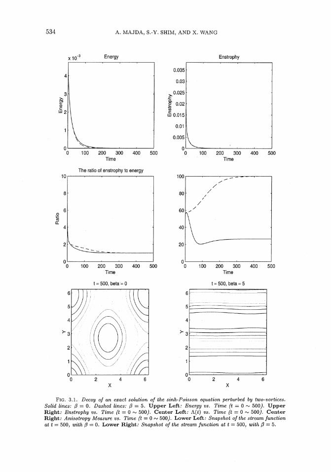
The initial data for the first simulation is a perturbation by two vortices of a special steady state solution to the inviscid problem with no /?-plane. These steady states are solutions of the so-called sinh-Poisson equation. For more detailed discus- sion about these solutions to the sinh-Poisson equation, the reader is referred to the original work of Ting, Chen and Lee (1987), or Majda and Holen (1998), or Grote and Majda (1998) or the book of Majda, Embid and Wang (1999). More specifically the initial data takes the form

2

(3.111) A^(f,0) =CJO =UJC,I + ÂA(|f-£i|),


where

(««> w>-{(1-(},,,;£:^ and

TT

(3.113) xi = (7r,7r),f2 = (T^71

")

(3.114) i4i =5, A2 = -5

(3.115) r = TT/IO

where c<;c?i is the vorticity of the sinh-Poisson solution. The initial Reynolds number is about 260. Figure 3.1 illustrates the numerical results on energy, enstrophy and Dirichlet quotient decay, Rhines measure for anisotropy and selective decay states with and without /?. We emphasize the difference in the measure of anisotropy and the difference in the geometric feature of the decay states. For the case with ft = 5 we observe complete anisotropy with zonal flow in the limit in contrast to /? = 0.

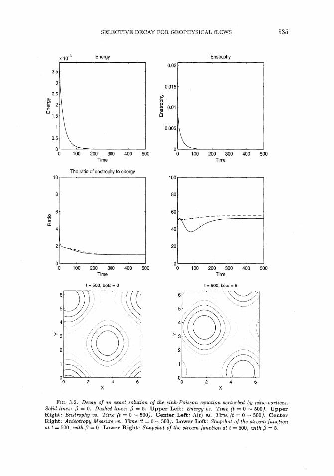
The initial data for the second simulation is a perturbation by nine random vortices of the same solution to the sinh-Poisson equation. The random vortices are of the same form and same magnitudes with random location and random radius. The initial Reynolds number is about 179. Figure 3.2 illustrates the numerical results on energy, enstrophy and Dirichlet quotient decay, Rhines measure for anisotropy and selective decay states with and without /?. This times the selective decay states with /? looks like horizontal translation of the selective decay states without /?, and for these initial data, the selective decay state shows no effect of /?.

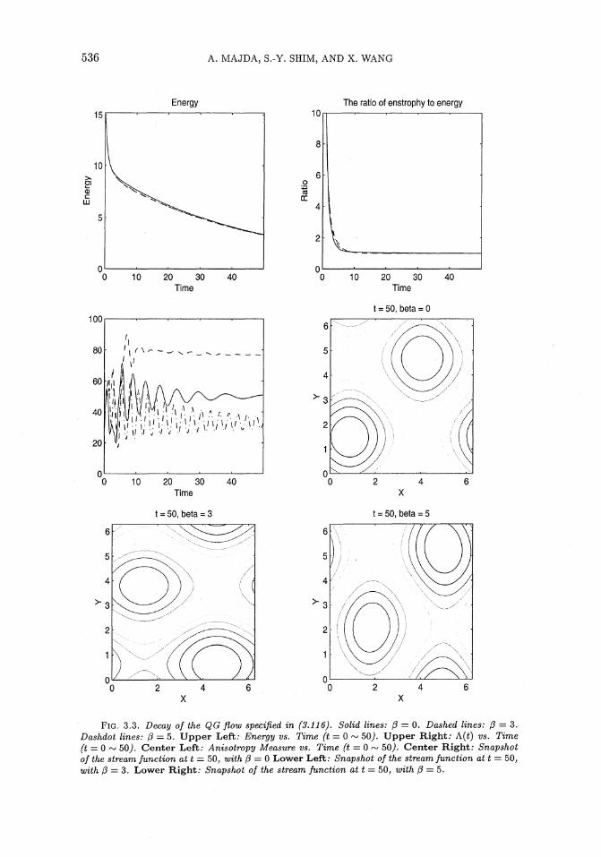
The initial data for the third simulation is the following stream function used by Rhines (1975)

(3.116) ^(£, 0) = cos(a; + 0.3) + 0.9 sm(3(y + 1.8) + 2x)

+0.87sin(4(x - 0.7) + {y 4- 0.4) + 0.815)

+0.8 sin(5(z - 4.3) + 0.333) + 0.7 sm(7y + 0.111)

Note that the various modes superimposed here result in a broad spectrum of the stream function. The initial Reynolds number is about 8046. Figure 3.3 illustrates the numerical results on the decay of energy, Dirichlet quotient (the difference in enstrophy decay is almost indistinguishable), Rhines measure of anisotropy for different f3 and the difference in geometric nature of the selective decay states for different values of /3. For /? = 3, the final state is roughly 75% zonal flow and has a large zonal jet. The cases with (3 — 0 and /? = 5 are more isotropic. These results point to very subtle development of zonal jets in the final state.

4. Selective Decay for Stratified Flows. The purpose of this section is to study the selective decay phenomena associated with stratified flows using either the continuously stratified model (2.6) or the two layer model (2.18). The situation with the continuously stratified model is quite subtle. In fact the validity of the selective decay principle depends on whether we have anisotropic diffusivity. In the case of isotropic diffusivity, the selective decay principle remains valid while for the


xKT Energy Enstrophy

0 100 200 300 400 500 Time

The ratio of enstrophy to energy

0 100 200 300 400 500 Time

t = 500, beta = 0

100 200 300 400 500 Time

uu - 1 1 ^ _!■ -- 1

/ 80

/ / / /

/ 60 /

40

X 20

n

0 100 200 300 400 500 Time

t = 500, beta = 5

2 4 X

FIG. 3.1. Decay of an exact solution of the sinh-Poisson equation perturbed by two-vortices. Solid lines: {3 = 0. Dashed lines: P = 5. Upper Left: Energy vs. Time (t = 0 ~ 500,). Upper Right: Enstrophy vs. Time (t — 0 ~ 500,). Center Left: A(t) vs. Time (t = 0 ~ 500). Center Right: Anisotropy Measure vs. Time (t = 0 ~ 500/ Lower Left: Snapshot of the stream function at t = 500, with (5 = 0. Lower Right: Snapshot of the stream function at t = 500, with {3 — 5.


x10"3 Energy

3.5

3

2.5

C

1.5

1

0.5

n

Enstrophy

100 200 300 400 500 Time

The ratio of enstrophy to energy

0 100 200 300 400 500 Time

t = 500, beta = 0

100 200 300 400 500 Time

0 100 200 300 400 500 Time

t = 500, beta = 5

FIG. 3.2. Decay of an exact solution of the sinh-Poisson equation perturbed by nine-vortices. Solid lines: /3 = 0. Dashed lines: 0 = 5. Upper Left: Energy vs. Time (t = 0 ~ 500/ Upper Right; Enstrophy vs. Time (t = 0 ~ 500/ Center Left: A(t) vs. Time (t = 0 ~ 500/ Center Right: Anisotropy Measure vs. Time (t = 0 ~ 500/ Lower Left: Snapshot of the stream function at t = 500, with (3 = 0. Lower Right: Snapshot of the stream function at t = 500, with (3 = 5.


Energy The ratio of enstrophy to energy

10 20 30 40 Time

10 20 30 40 Time

100

20

60

i-1

h 4U Kirii': I 't :\ 'I •' :\ ,.

';/'■ /^ • !• r- A

!;!;';\/"VV^^-'VvV^

0 10 20 30 40 Time

t = 50, beta = 0

t = 50, beta = 3 t = 50, beta = 5

FIG. 3.3. Decay of the QG flow specified in (3.116). Solid lines: (3 = 0. Dashed lines: (3 = 3. Dashdot lines: (3 = 5. Upper Left: Energy vs. Time (t = 0 ~ 50). Upper Right; A(t) vs. Time (t = 0 ~ 50). Center Left: Anisotropy Measure vs. Time (t = 0 ~ 50). Center Right: Snapshot of the stream function at t = 50, with (3 = 0 Lower Left; Snapshot of the stream function at t = 50, with (3 = 3. Lower Right; Snapshot of the stream function at t = 50, with (3 = 5.

|2


anisotropic diffusivity case we have an explicit counter-example indicating the failure of the selective decay principle. For the two layer problem, the selective decay principle is never valid and it is also illustrated via explicit counter-examples.

Recall that the energy for the continuously stratified model is defined as

(4.1) jB=iy(|v^|2 + JF2|^|2),

and the corresponding enstrophy is defined as

(4.2) e=1„J\Alp + F2^1pf

The generalized Dirichlet quotient is defined as

(«) A«) = ||.

We have the following theorem

THEOREM 2. Selective decay of the continuously stratified quasi- geostrophic flows For the continuously stratified quasi-geostrophic equations (2.6) the following are true

(A) Selective decay with special parameter //

(4.4) Pr = F2 = 1,

then the selective decay principle holds. More precisely, the generalized Dirichlet quotient monotonically decreases to some eigenvalue of the three dimensional Laplacian and all flows approach asymptotically to the superposition of Rossby waves and a steady state zonal flow.

(B) Failure of selective decay with anisotropic vertical diffusion //

(4.5) Pr • F2 £ 1

then the selective decay principle fails. More precisely , we can build explicit counter-examples consisting of superposition of a Rossby wave and a vertical shear such that the generalized Dirichlet quotient increases as time evolves.

(G) Failure of selective decay for two layer model For the two layer quasi- geostrophic model (2.18), the selective decay principle fails for all geophysical parameters F ^ 0.

In the special case of exact balance of stratification and rotation i.e., F — 1 the theorem leads to

COROLLARY 1. In the special case of exact balance of stratification and rotation, i.e.

(4.6) F = 1

the necessary and sufficient condition for the validity of the selective decay principle for the continuously stratified quasi-geostrophic flows (2.6) is

(4.7) Pr = 1,


or the kinematic viscosity equals to the thermal diffusivity.

We separate the proof of the theorem into two parts. In subsection 4.1 we con- struct explicit counter-examples illustrating the failure of the selective decay principle for the continuously stratified quasi-geostrophic model with anisotropic diffusivity (4.5). We also present an explicit counter-example illustrating the failure of the selective decay principle for the two layer model. In section 4.3 we sketch the proof of the selective decay with isotropic diffusion.

4.1. Counter-examples to Selective Decay with Vertical Anisotropic Diffusivity. We consider a counter-example taking the form of a Rossby wave plus a vertical shear, namely

(4.8) ip(x, z, t) = e-At sm(lx + 0t/l) + coe'31 sin(fcz/0)

With this ansatz, we see that

(4.9) A^ + F2|^ = -l2e-Atsm{lx + pt/l) - (^)2F2coe-Bt sin(]fez/0),

and

(4.10) J(Â^ + F2 J^/OÔ.

Thus for this special ansatz, the continuously stratified quasi-geostrophic equation (2.6) with dissipation operator in (2.8) takes the form

(4.11) Al2e-At sm(lx + 0t/l) + B(^)2F2coe-Bt sm(kz/Q)

-l(3e-At cos(lx + pt/l) + I0e-At cos(lx + 0t/l)

= -^r(l4e-At sm(lx + pt/l) + (^)4CoPr-1F2e-Bt sin(Jfez/0)). Re K)

This implies

Al2=Re-1l4,

B(^)2F2=Re-1(^)4Pr-1F2.

This is equivalent to

(4.12) A = l2/Re;

(4.13) B = (t)2/(Re-Pr).

We thus conclude that the ansatz (4.8) gives exact solution to the continuously stratified quasi-geostrophic equations (2.6) with arbitrary choice of/, k and the special choice of A,B given by (4.12) and (4.13).

Now for this chosen ansatz we compute the energy, enstrophy, generalized Dirich- let quotient and its dynamics.

d2

(4.14) 2S{t) = Ji&iP + F2^)2

= [(-Pe-At siniix + ^/i) _ ^jtiê-Bt sin ^)

= h^Qil'e-^ +c2F\^)ie-2Bt)


(4.15) 2E(t) = - JÂ^ + F2^)

= - f{e-At sm(lx + fit/I) + coe-Bt sin ^)

(-/2e-Ai sm{lx + dt/l) - c0JF2(|)2

e-B' sin ~)

= h^Q{l2e-2Ai + c2F2(i)2e-2B()

and hence

(4-16) A(t) = 4 E _l4e-2M+clF4(±)4e-2m

- l2e-2At+c2F2^2e-2Bt

= l2 l + c2(Ek)ie-2(B~A)t

l + c2(^)2e-2(B-^ ,1 +f2f

= ZJ ;l + ^(w)4e'2(B"A)f

den

where

(4.17) den = 1 + cl{ê-2(B-A)t

Hence

^"U^npr-Hh2 - '2)((S)2 - i)«2(A-B)t den2RexlQ' v v0' MV/e

_ 2/ C0 ,Ffc,2, fc IW^S2 1\ 2(^-.B)t denêWe^ l02;2Fr ;u/0; ;

Under the anisotropic vertical difFusivity assumption (4.5) we either have

(4.19) FPr* > 1

or

(4.20) FPr* < 1.

Since we have the freedom of choosing I and k, we can choose these two integers so that their rational ratio is approximately,

(4.21)

This implies

(422) m^PrPrhF'

(4-23) {Ehf^pr\R

k2

e2i2 Pri F

k2 1


When these estimates are combined with (4.18) and either (4.19) or (4.20) we have

(4.24) JtA^>0-

Hence the selective decay principle fails here.

4.2. Counter-examples to selective decay for the two layer model with arbitrary parameters. In this subsection we present a counter-example to selective decay for the two layer model (2.18) with arbitrary parameters with the same diffusivity from (2) acting on each layer. The example we have in mind is the superposition of a barotropic Rossby wave and a baroclinic Rossby wave of the form

(4.25) </>i = e~At sin(z + fit) + e-23' cos(£ + fit),

(4.26) </>2 = e"A* sm(x + fit) - e'31 cos(z + fit)

with the constants A, B given by k

(4.27) A = YJdj, J=I

(4-28) B = E2Î-

It is easy to check that this is an exact solution to the two layer model (2.18). The sin part of the solution is the barotropic component and the cos part of the solution is the baroclinic component.

The energy and enstrophy of the flow can be calculated easily as

(4.29) E(t) = \{e-2At + (1 + 2F)e-2Bt) x 47r2,

(4.30) £{t) = \(e-2At + (1 + 2F2)e-2Bt) x 47r2.

Thus the generalized Dirichlet quotient takes the form

e-2At + (1 + 2F2)e-2Bt

- e-2At + (l + 2F)e-2Bt

el+(l+2.F2)e-2<B-A"

= 1 + (1 + 2F)e-2(B-^t

Hence we deduce, via direct differentiation,

d 2F{2F + l)2{A-B)e2^-^ ^■6Z) dt [) ~ (1 + (1 + 2F)e-2(s-A)t)2

Since

(4-33) A-B = ^FTlJ2d^>0

3=1

we conclude that selective decay fails for F > 0. The physical mechanism behind this failure of selective decay is again

the anisotropy of diffusivity. Notice for the barotropic part ^(V>i +^2) the dissipation rate is A while for the baroclinic part |(î - ^2) the dissipation rate is B.


4.3. Proof of Selective Decay with Special Parameters. In this subsection we give a sketch of the proof of the validity of the selective decay principle for the continuously stratified quasi-geostrophic model (2.6) with special choice of parameters given in (4.4). We will give a proof of the decay of the generalized Dirichlet quotient only. The fine detail of convergence and long time behavior can be derived in pretty much the same fashion as in subsection 3.1. We omit the details here.

For the special choice of parameters (4.4) we have

(4.34) E = ±j\V3ip\2,

(4.35) £=i||A3V|2.

The time evolution of energy and enstrophy are given by

(4.36) ^(i) = -JRe-1||A3^||^

(4.37) |5(t) = -iJe-1||(-A3)Mlo-

Thus

d k' d £(t)

1 -X^m - m^-rn)) E(tydt w wete

1 "'(-A3)^-A(t)(-A3)^llg E(t)ReKUK *' r wv OJ2

+A(*)(||A3^||2-A(*)||(-A3)^||2))

:(||(-A3)i^-AW(-A3)^). E{t)ReyuK *' * wv OJ2

This proves the decay of the Dirichlet quotient under the assumption on special parameters (4.4). The case with hyper-viscosity can be treated in pretty much the same way as in the proof of Lemma 1.

4.4. Ground States. We now focus on computing the ground states since these are the long time behavior of the continuously stratified model under this special parameter choice and generic initial data.

It is easy to see that the eigenvalues of the three dimensional Laplacian takes the form

(4.39) kl + kl + 02/c!, kl + kl> 0,

where kj are integers. The non-degenerate condition k\ + k^ > 0 is to ensure that we do not have a flow with zero velocity field. This is also equivalent to impose the zero mean in the horizontal (#, y) average. Of course the zero horizontal mean is preserved


under the dynamics of the continuously stratified quasi-geostrophic equation (2.6). It is then easy to see that the first eigen value is

(4.40) Ai = 1,

and the ground energy shell has the base

(4.41) sin x, cos x, sin y, cos y.

This is the same situation as for the one layer model (2.1). Thus the long time dynamics of the continuously stratified quasi-geostrophic equations with dissipation and special choice of parameters (4-4) is independent of the vertical direction. In fact the long time dynamics coincides with that of the one layer model, i.e., a superposition of a zonal flow and two Rossby waves.

5. Selective Decay for Flows on Sphere. In this section we study the selective decay phenomena related to the barotropic quasi-geostrophic equation, or the one layer model on sphere. The study of flows on sphere is of great importance due to the geometry of the earth and other planets.

5.1. The Basic Equation and Some Useful Calculus on Sphere. In this subsection we introduce the barotropic quasi-geostrophic equations (one layer model) on sphere. We also recall some useful calculus formulas on sphere for the purpose of the understanding the proof of our theorems below.

We first recall the basic dynamic equations, the barotropic quasi-geostrophic equations on the unit sphere S2 in surface spherical coordinates 0, 0, with 0 being the longitude and 0 being the latitude

(5.1) ^ + JW>, A^ -I- 2fi sinfl) - P(-A)^,

where if; is the stream function, A is the Laplace operator on scalars on the unit sphere,

k

(5.3) 2>(-A) = £<*,■(-A)', ^>0, 3=1

(5.4) q = Ail; + 2fLsm0

is the potential vorticity. The barotropic quasi-geostrophic equations on the unit sphere can be written in

terms of the potential vorticity

^ + J(^q)=V(-A)ij.

It is easy to see that the mean of the stream function Js2 ip does not play any role in the dynamic equations. Hence without loss of generality we may assume that the stream function has zero mean, i.e.

(5.5) [ rl> = 0. s2


Thus we may recover the stream function from the vorticity UJ or the potential vorticity q by solving the Laplace equation

Aif) = LJ = q — 2fl sin 9,

together with the zero mean condition on ip. We also notice that

(5.6) JOMin0) = ||,

and hence we may rewrite the basic dynamic equation as

(5.7) ^ + j(V,iAV,) + 2fi^=P(-A)</>.

This form of the barotropic quasi-geostrophic equation on the unit sphere is very much the same as the one in the flat geometry case introduced in section 2.1 except the horizontal independent variable x is replaced by the longitude variable </>. Thus we could expect similar behaviors of solutions for the two different cases. In particular we are able to prove that the selective decay principle remains valid for barotropic quasi-geostrophic flows on sphere. However due to the difference in symmetry groups, we will also witness difference in solution behaviors. In particular there is very special nonlinear dynamics on the subspace spanned by the first two eigenspaces as we indicate in section 5.2.

5.1.1. Common Differential Operators and Integration by Parts For- mulas on the Sphere. For the sake of convenience we list here some of the commonly used differential operators and integration by parts formulas on the sphere. These are standard materials and can be found in any standard textbook on differential geometry.

The surface element on a sphere with radius a is

(5.8) ds = a2cosed(f)d6.

At each point of the space (outside 9 = —7r/2 or 7r/2), we define the usual local orthonormal system, {e^, ee}, corresponding to increasing values of </> and 0. We define ft = er as the unit vector corresponding to the increasing values of the radius.

Let ip be a scalar field on S2 and v = vê^ -f veee be a tangent vector field on S2. We recall several common differential operators and integration by parts formulas on the sphere. The gradient operator on scalar field is defined as

5.9 W> = grad </> = -ê0 + -^^. a cos 0 ocj) a 80

The perpendicular gradient operator, or the curl operator on A scalar field is defined as

(5.10) V^ = curl ^ = VV> x ft = -jê^ ^757^. a 80 a cos 0 ocf)

The divergence operator on vector field is defined as

V5-11) div v = V • i; = --~f + ^ . a cos 0 ocj) a cos 0 00


(5.12) curl v = div (v x n) = -jr- ^-^Z "• acosv ocp a cos 6 ov

The Laplacian operator on scalar field is defined as

(5.13) A^ = div grad ^ = - curl curl ^ = —2 ^{ ^^TT + ^(cos6,^•)}• a2 cos 8 cos 6 a</>2 a^ a^

We recall here one of the alternative definitions of Av, i.e. the Laplacian operator for tangential vector fields on the unit sphere

(5.14) Av = grad div v— curl curl v

-/A 2sinfl dve v^ ^ f 2sin<9 dv^ VQ

~ i * a?cos>e dcj) a2cos2ê0 + i *a2cos20 d(j) a^cosÔ^9'

We also recall Stokes formulas

(5.15) / div v ipds = — / v- Vilids, Js2 Js2

(5.16) / curl v ifids —I v- curl ipds, Js2 Js2

(5.17) - / Aip'ipds = - / Â^rfs = / V^ • V^^5, Js2 Js2 Js2

(5.18) -/ Av-$ds= / (Vif-V^+-o-tf-i7)ds.

5.1.2. Eigenfunctions of the Laplacian operator and the Legendre functions. As in the flat geometry case, the Laplace operator will play an important role in studying the behavior of solutions to the barotropic quasi-geostrophic equations on the unit sphere (5.1). For the doubly periodic domain we have witnessed that the eigenfunctions of the Laplacian operator, the trigonometric functions, played an essential role in our analysis of the behavior of solutions. For spherical geometry, the trigonometric functions are replaced by the following Legendre functions

(I _ ^2\f Am+nM _ z2\n (5-19) Pnm(Z) = [-^J d

[zn+m ) , for 0 < m < n.

These functions enjoy the following orthogonal property:

2 (n+ 771)!. (5.20) / Pnm(z)Pntm(z)dz =

2n + l (n-ra)!

The eigenfunctions of the Laplacian operator on the unit sphere can be repre- sented using the Legendre functions. Indeed the eigenvalues must be in the set

(5.21) {-n(n + l) | n G Z+}


and for each eigenvalue — n(n + 1) the associated eigenfunctions are

(5.22) Pnm(sm9) exp(im^), for 0 < m < n.

or their normalized form

(5.23) Ynrn = A^nmPnm(sin^) exp(im^),

where

_,(2n + l)(n-H)!a ivnm-t ■47r(n + |m|)! ; »

or their real valued form (not normalized)

(5.24) wn = Pn(sin0),

(5.25) Wanm = Pnm(sin^) cos(m0);

(5.26) ^nm = Pnm(sin0) sin(m^);

for 1 < m < n. Roughly speaking, these functions will replace the trigonometric functions in this

spherical geometry.

5.2. Exact Nonlinear Dynamics on the First Two Eigenspaces. In this section we present the exact nonlinear dynamics of the barotropic quasi-geostrophic equations on sphere with dissipation (5.1) on the first two eigenspaces, i.e. all eigenfunctions corresponding to the eigenvalues -2 and -6.

Due to the special geometry of the sphere, the dynamics on the first eigenspace (corresponding to -2) is independent of the motion of higher eigenspaces. The first two eigenspaces form an invariant subspace of the whole dynamics. We recall the exact dynamics here and leave the proof in the Appendix.

For exact solutions which span the first two eigenspaces, this will delineate some special structure of solutions with spherical geometry and also yield two natural versions of selective decay.

5.2.1. Independent Dynamics on the First Eigenspace. We recall (see subsection 5.1.2) that the first eigenspace (corresponding to the eigenvalue -2) has a basis of the form

(5.27) wi = sin 9

(5.28) Wall = cos 6 COS (j),

(5.29) Wbn — cos6sm(p.

The dynamics on the first eigenspace is given by

(5.30) dai 3 v^ . oi

3=1

(5.31)

(5.32)

546

for

A. MAJDA, S.-Y. SHIM, AND X. WANG

ift = alWl+all'Wan+bllWbn+'lp, = ai(t)sm9+aii(t)cos6cos(l)+bii(t) cos8sin(j)+1/1' (5.33) with

(5.34) Ip' _L Wx , Ip' ± Wall, i/)' -L ^611 •

The solutions can be written out explicitly as

l(*) = ai(0)c-*^1di2i*j (5.35) Gil

011W = (aii(O) cos(m) 4- 6ii(0) sin(nt))e 8- ^=1 dj23\ (5.36)

(5.37) ftnW = (-aii(O) sin(m) + bnfi) cos(fi*))e"* ^-^ dj23t

Thus the projection onto the first eigenspace of the stream function takes the form

(5.38) e~^ £;=i di2,t(ai(0) sintf + aii(O) cosl9(cos(nt) cos^ - sin(fit) sin^)

+611 (0) cos ^(sin(n^) cos (f> + cos(fl£) sin </>))

+011 (0) cos 9 cos(ftt + </>) + bn (0) cos 0 sin(fi* + 0))

and the associated velocity field takes the form

(5.39) E:=1^ (ai(O)(cos0,O) 4-aii(0)(- sini9cos(0^ + 0), - sin(ni + 0))

+611 (0)(- sin 19 sin(n^ + 0), cos(^ + (/>))).

This implies that the velocity field we have is a zonal flow plus two Rossby waves. These Rossby waves travel in the opposite direction to the earth's rotation with the same velocity magnitude as the rotation.

Since the dynamics on the ground energy shell is independent of motion on higher energy shells, we see that the space spanned by all eigenspaces except the first one is invariant under the barotropic quasi-geostrophic dynamics (5.1).

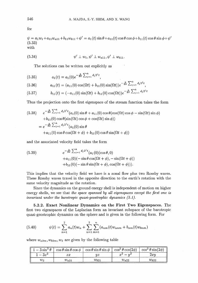
5.2.2. Exact Nonlinear Dynamics on the First Two Eigenspaces. The first two eigenspaces of the Laplacian form an invariant subspace of the barotropic quasi-geostrophic dynamics on the sphere and is given in the following form. For

2 2 n

(5.40) 1p(t) = ^ anifiWu + XI S (anm WWanm + bnrn{t)whnm) n—1 n=l 77i=l

where Wa2m,'Wb2m,W2 are given by the following table

l-3sin2<9 cos 9 sin 9 cos (j) cos 9 sin 9 sin (j) cos2 9 cos (20) cos2<9sin(20) 1-Sz2 zx yz sa-l/* 2xy

W2 Wa21 Wb21 Wa22 Wb22


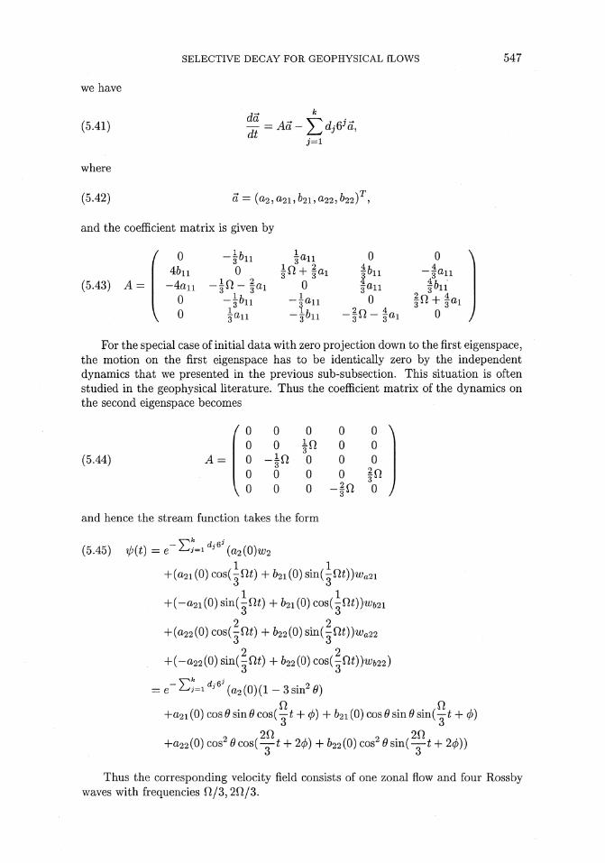
we have

(5.41) 7-> K

where

(5.42) o = (02,021,621, a22,b22)T,

and the coefficient matrix is given by

(5.43) A =

( 0 4&ii

-4aii 0

V 0

-5611 0

-ift-fai -i&n |aii

3aii |n + |oi

0 — gfflll

-j6ll

0 LI

3-aii f6»

3^ roi

0 — 3ai1

I&11 ffi + fo!

0 /

For the special case of initial data with zero projection down to the first eigenspace, the motion on the first eigenspace has to be identically zero by the independent dynamics that we presented in the previous sub-subsection. This situation is often studied in the geophysical literature. Thus the coefficient matrix of the dynamics on the second eigenspace becomes

/ 0 0 0 0

(5.44) A =

0

0 -|ft 0 0 0

V 0 0

0 0 0

0 0 2

2

0 \ 0 0

3" 0 -ffi 0 /

and hence the stream function takes the form

(5.45) ^(t) = eT £*-» dj'6J (O2(0)w;2

+(021(0) cos(-m) + &2i(0)sin(-Oi))wa2i

+(-021(0) sin(-m) + 621(0) cos(-fii))w62i

+(022(0) cos(-nt) + 622(0) sin(-m)K22

2 2 + (-022(0) Sin(-nt) + 622(0) COS(-fit))«'622)

= e- Ej=id^ (a2(0)(l - 3 sin2 0)

+021(0) cos#sin#cos(—t + (/>) + 621(0) cos0sin0sin(—t + </>)

-f 022(0) cos2 <9 cos(—t + 20) + 622 (0) cos2 (9 sin(—* + 20))

Thus the corresponding velocity field consists of one zonal flow and four Rossby waves with frequencies fi/3,20/3.


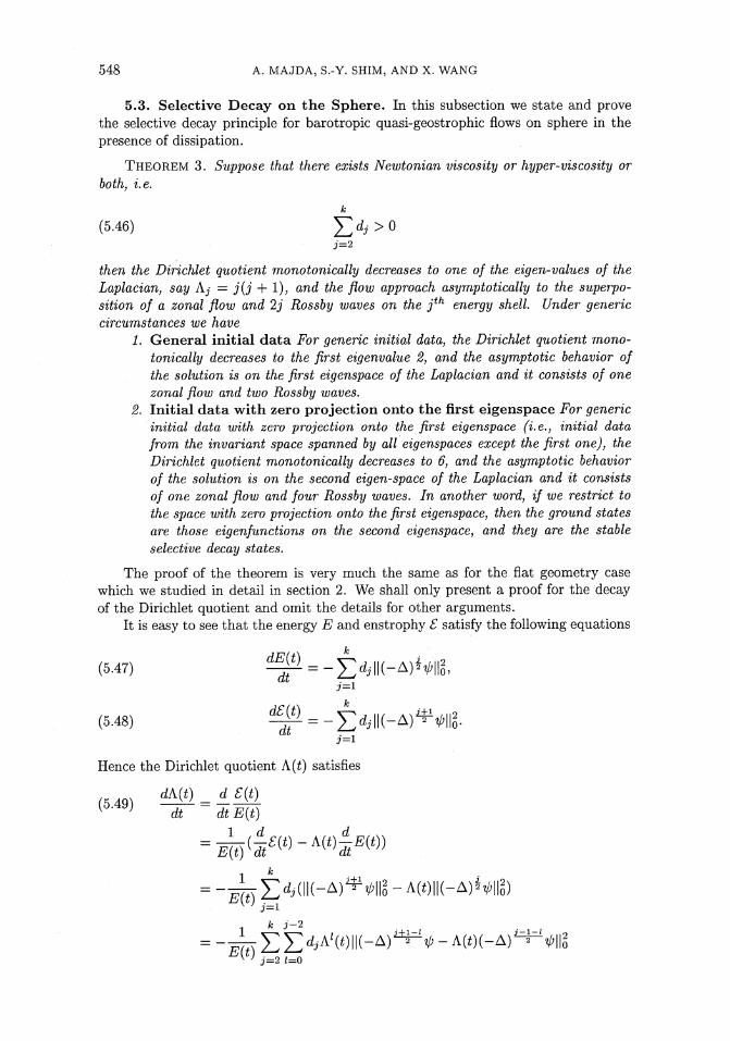
5.3. Selective Decay on the Sphere. In this subsection we state and prove the selective decay principle for barotropic quasi-geostrophic flows on sphere in the presence of dissipation.

THEOREM 3. Suppose that there exists Newtonian viscosity or hyper-viscosity or both, i.e.

k

(5.46) E^>0

i=2

then the Dirichlet quotient monotonically decreases to one of the eigen-values of the Laplacian, say Aj — j(j + 1), and the flow approach asymptotically to the superposition of a zonal flow and 2j Rossby waves on the jth energy shell. Under generic circumstances we have

1. General initial data For generic initial data, the Dirichlet quotient monotonically decreases to the first eigenvalue 2, and the asymptotic behavior of the solution is on the first eigenspace of the Laplacian and it consists of one zonal flow and two Rossby waves.

2. Initial data with zero projection onto the first eigenspace For generic initial data with zero projection onto the first eigenspace (i.e., initial data from the invariant space spanned by all eigenspaces except the first one), the Dirichlet quotient monotonically decreases to 6, and the asymptotic behavior of the solution is on the second eigenspace of the Laplacian and it consists of one zonal flow and four Rossby waves. In another word, if we restrict to the space with zero projection onto the first eigenspace, then the ground states are those eigenfunctions on the second eigenspace, and they are the stable selective decay states.

The proof of the theorem is very much the same as for the flat geometry case which we studied in detail in section 2. We shall only present a proof for the decay of the Dirichlet quotient and omit the details for other arguments.

It is easy to see that the energy E and enstrophy £ satisfy the following equations

(5.47) « = _2di||(_A)MlS.

d£(t)

dt . ,

(5.48) ^ =-Em-^^wi

Hence the Dirichlet quotient A(t) satisfies

dA(t) d £{t) (5.49)

dt dt E{t) 1 -{±£(t)-k(t)±-E{t))

E{tydt w v ' dt

-l^£^(ll(-A)^l§-A(t)||(-A)Ml§) m î k 7—2

££diA'(t)||(-A)iti=iV-A(«)(-A)i=î^||g *(«)££


where we have used the same recursive argument (3.32) with C = A(£) as in the proof of Lemma 1.

This completes the proof of the decay of the Dirichlet quotient.

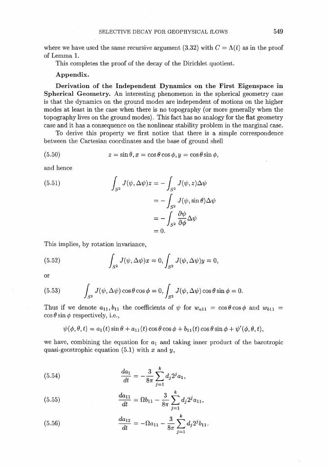
Appendix.

Derivation of the Independent Dynamics on the First Eigenspace in Spherical Geometry. An interesting phenomenon in the spherical geometry case is that the dynamics on the ground modes are independent of motions on the higher modes at least in the case when there is no topography (or more generally when the topography lives on the ground modes). This fact has no analogy for the flat geometry case and it has a consequence on the nonlinear stability problem in the marginal case.

To derive this property we first notice that there is a simple correspondence between the Cartesian coordinates and the base of ground shell

(5.50) z = sin 0, x = cos 6 cos 0, y = cos 8 sin </>,

and hence

(5.51) / J(ip,Aip)z = - [ J{ip,z)Aip Js2 Js2

= - / Jft/ssinflJA^ Js2

= - [ w Js2 Is2 OQ

= 0.

This implies, by rotation invariance,

(5.52) [ Jty, A</0* = 0, / Jty, A^)y = 0, Js2 Js2

or

(5.53) / J(^, Aip) cos 6 cos </> = 0, / J(^, A^) cos 6 sin </> = 0. Js2 Js2

Thus if we denote an,feu the coefficients of ip for Waii = cos9cos0 and Wbn — cos6sin (f) respectively, i.e.,

il){<j),0,t) = ai(£)sin0 4- aii(t)cos0cos0 + bnCOcosflsin^ + ^'^fl,*),

we have, combining the equation for ai and taking inner product of the barotropic quasi-geostrophic equation (5.1) with x and y,

(5.54)

(5.55)

(5.56)

dai

dt

dan dt

= nbll-—yjdj2:>all,

dau dt

= -001!- —);diy'6i1


This implies that the motion on the ground states is independent of motion on higher energy shells, and it consists of a zonal flow and two Rossby waves.

This is in contrast to the flat geometry case where we have the first energy shell an invariant subspace of the dynamics. However if the initial data contains modes outside the ground energy shell future dynamics on the ground energy shell will have interaction with higher modes in the flat geometry case.

Derivation of the Exact Nonlinear Dynamics on the First Two Eigen- spaces in Spherical Geometry. It is known that each energy shell (eigenspace), i.e., all eigenfunctions associated with one fixed eigenvalue of the Laplacian operator, is invariant under the barotropic quasi-geostrophic equation without forcing in the flat geometry since the Jacobian drops out in this special case. This is also true for the sphere geometry. Moreover we are able to deduce more invariance due to the special sphere geometry of the sphere. We observe from the computation above that the interaction (through the nonlinear convection term) of z — sin # with other eigenfunctions is to make a rotation of 90° around the z axis combined with a scalar multiplication. Similar results hold for x — cos 9 cos (f) and y = cos 9 sin 0. This is easily generalized to eigenfunctions corresponding to higher eigenvalues (An,n > 2). And if we consider the dynamics on the space spanned by all eigenfunctions corresponding to the eigenvalues Ai and An (for fixed n), we will see that this form an exact nonlinear dynamics of the full quasi-geostrophic equations in the absence of topography. These exact dynamics exhibit periodic and possible quasi-periodic motions. This phenomena is not present for the flat geometry even if we make the analogy between the ground shell motion in the spherical geometry case to the large mean motion in the flat geometry case. Notice we always have nonlinear dynamics on the first two shells for the spherical geometry case while we have nonlinear dynamics for the flat geometry case only if there is nontrivial topography.

To derive the exact dynamics on the first eight eigenfunctions, or the first two shells, we start with the following simple observation

bnm-) (5.57) J(Wanm, z) = -mwb7]

(5.58) J(wbnm,z) = mWanm,

(5.59) J(wn,z) = 0.

Denoting

(5.60) Wn = span{wn,wanm,w&nm,l <m < n},

the nth energy shell, or the nth eigenspace, we have

(5.61) J(^n, Z) e Wn, if ^n € Wn.

Thanks to the rotation symmetry, the same result holds with z replaced by x or y, i.e.,

(5.62) J(^n, X) G Wn, J(^n, V) e Wn, if ^n G Wn.

This implies

(5.63) JW>n,0l) € Wn, if ^n € Wn, </>l € Wi.

Now let

(5.64) ^ = ^1+^^ Wi+Wn,


with î G Wi^n E Wn, we have

(5.65) J(^, A^) = J(î + ^n, -2î - n(n + l)^n)

= -n(n + l)J(î,^n) - 2J(ipn,ipi)

= (n(n + l)-2)J(^n,î)

This proves that the dynamics on Wi + Wn is an exact dynamics for the original equation (in the absence of topography).

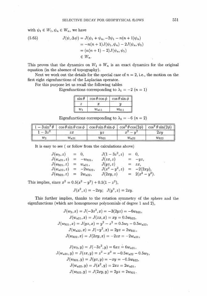
Next we work out the details for the special case of n = 2, i.e., the motion on the first eight eigenfunctions of the Laplacian operator.

For this purpose let us recall the following tables Eigenfunctions corresponding to Ai = -2 (n = 1)

sin0 cos 6 cos cj) cos 9 sin <f) z X y

W! Wall Wbll

Eigenfunctions corresponding to A2 = — 6 (n = 2)

l-3sin20 cos 8 sin 9 cos 0 cos ^ sin ^ sin 0 cos2^cos(20) cos2 6> sin(20) l-3z2 zx y* x'-y* 2xy

W2 Wa21 ^621 /Wa22 ^622

It is easy to see ( or follow from the calculations above)

J(w2,z) =0, J(l-Sz2,z) = 0, «/(tya2i,^) = -W&21, J(zx,z) = -yz, J{Wb21,z) = Wa21, J{yZ,z) = ^X, J(â22,^) = -2w;6225 J(x2-y2,z) = -2(2x2/), J(wb22,z) = 2iya22, J(2xy,z) = 2(a;2-2/2).

This implies, since x2 = 0.5(a:2 - y2) + 0.5(1 - z2),

J(x2,2) = -2a:t/; J(2/2, *) = 2xy.

This further implies, thanks to the rotation symmetry of the sphere and the eigenfunctions (which are homogeneous polynomials of degree 1 and 2),

J(w2,x) = J(-32;2,x) = -S(2yz) = -6W&21,

J(wa2i,x) = J(zx,x) = xy = Q.5wb22,

J(wb2i,x) = J{yz,x) — y1 - z2 = 0.5u;2 - 0.5'â22,

«/(wo22,a?) = J(-y2,x) = 2yz = 2wb2i,

J('Wb22,x) = J(2xy,x) = -2zx = -2w02i,

J{w2,y) = J(-3z2,y) = 6xz = 6iy02i,

J{'Wa2i,y) = J{zx,y) - z2 - X2 - -0.5^22 - 0.5^2,

J{wb2i,y) = J{yz,y) = -xy = -0.5^22,

J(Wa22,y) - J(x2,y) = 2X2 = 2â21,

J(wb22:y) = J(2xy)y) = 2yz = 2w62i.


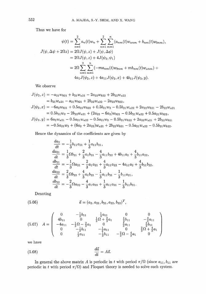
Thus we have for

^W - Yl anitfWn + X! XI (anm{t)wanm + bnm(t)wbnm), n=l n=l m=l

J(</>, A^ + 20^) = 20 J(^, ^) + J(^, A^)

= 2fiJ(^,z) + 4J(^2,^1) 2 n

= 2fi 5Z 5Z (-manm(t)wbnrn + mbnrn(t)wanm) + n=l m=l

4aiJ(^2,^) +4aiiJ(V>2,z) +46iiJ(^2,2/).

We observe

J{^2,Z) = -^21^621 + 621ô21 - 2a22W&22 + 2622'â22

= b2lWa21 - a<2l'Wb21 + 2622â22 " 2a22^&223

J(lp2,x) = -6a2^621 + 0.5a2llf;622 + 0.5&21W2 - 0.5621â22 + 2a22^621 - 2622'â21

= 0.5621^2 - 2&22â21 + (2a22 - 6a2)w&21 - 0.5621^22 + 0.5021^622,

J{^2,y) = 6a2Wa21 — 0.5a21â22 - 0.5a2lU>2 — 0.56211^622 + 2a22â21 + 2b22Wb21

= -0.5a2iif;2 + (602 4- 2a22)w;a2i + 2&22W&21 - 0.5a2iWa22 - 0.5621^622.

Hence the dynamics of the coefRcients are given by

da2 1 1 -rr - -^hiî + -aii&2i, at 6 0

da2i 12 4 4 —— = -ftfoi + oai&2i - oaii622 + 46iia2 + -611022,

—— = --S2a2i - -01021 + -011022 - 4aiia2 + 0^11^22, at o o o o

â22 2 4 1 1 -^7- = o J^22 + oal&22 - oall621 " o&lla2l5

^22 20 4 a.1 ^ 7, —rr = -oâ22 - oaia22 + -aiia2i - -O11O21. at 3 6 6 0

Denoting

(5.66) a = (a2,a2i, 621,0^22,622)T,

(5.67) A =

we have

(5.68)

/ 0 4&ii

-4aii 0 0 V

0 ■in-fax

|oii

3O11

in + fd 0

-|aii

-hn

da — = Aa. dt

0

3all 0

|6ii ffi + fo!

In general the above matrix A is periodic in t with period ir/Ct (since an, 611 are periodic in t with period TT/O) and Floquet theory is needed to solve such system.


Acknowledgments. Andrew Majda is partially supported by NSF grants DMS- 9625795 and DMS-9972865, ARO grant DAAG55-98-1-0129, and ONR grant N00014- 96-0043. Wang acknowledges the partial support of a Faculty Development Fund from the Iowa State University. The decay of the Dirichlet quotient in the case without F-plane but with hyper-viscosities was first discovered by Zhou-Pin Xin.

REFERENCES

[1] H. BREZIS AND T. GALLOUET, 1980, Nonlinear Schrodinger evolution equations, Nonlinear Anal., TMA, 4, pp. 677-681.

[2] P. CONSTANTIN AND C. FOIAS, 1988, Navier-Stokes Equations, Chicago University Press, Chicago.

[3] O. EMBID AND A. MAJDA, 1998, Low Froude number limiting dynamics for stably stratified flow with small or finite Rossby numbers, Geophys. Astrophys. Fluid Dynamics, 87, pp. 1-50.

[4] C. FOIAS AND SAUT, 1984, Asymptotic behaviour, as t —>■ oo of solutions of Navier-Stokes equations and non-linear spectral manifolds, Indiana Univ. Math. J., 33, pp. 459-477.

[5] C. FOIAS AND R. TEMAM, 1989, Gevrey class regularity for the solutions of the Navier-Stokes equations, J. Funct. Anal., 87, pp. 359-369.

[6] A. E. GILL, 1982, Atmosphere-Ocean Dynamics, Academic Press, New York. [7] M. GROTE AND A. MAJDA, 1997, Crude closure dynamics through large scale statistical theory,

Physics of Fluids, 9, pp. 3431-3442. [8] J. HALE, 1988, Asymptotic Behavior of Dissipative Systems, Mathematical Surveys and Mono-

graphs, vol. 25, AMS, Providence. [9] A. MAJDA AND A. BERTOZZI, 1999, Vorticity and the Mathematical Theory of Incompressible

Flow, Cambridge University Press, Cambridge, England, To appear. [10] A. MAJDA, P. EMBID, AND X. WANG, 1999, Nonlinear Dynamics and Statistical Theory for

Basic Geophysical Flows, in preparation, based on lectures by A. Majda at the Courant Institute in 1995, 1997, 1998.

[11] A. MAJDA AND M. HOLEN, 1998, Dissipation, topography, and statistical theories for large scale coherent structure, CPAM, vol. L, pp. 1183-1234.

[12] W. H. MATTHAEUS AND D. MONTGOMERY, 1980, Selective decay hypothesis at high mechanical and magnetic Reynolds numbers, Annals New York Academy of Sciences, pp. 203-222.

[13] W. H. MATTHAEUS, W. T. STRIBLING, D. MARTINEZ, S. OUGHTON, AND D. MONTGOMERY,

1991, Decaying two-dimensional Navier-Stokes turbulence at very long times, Physica D, 51, pp. 531-538.

[14] D. MONTGOMERY, X. SHAN, AND W. H. MATTHAEUS, 1993, Navier-Stokes relaxation to sinh- Poisson states at finite Reynolds numbers, Phys. Fluids A, 5:9, pp. 2207-2216.

[15] D. MONTGOMERY AND G. JOYCE, 1974, Statistical mechanics of negative temperature states, Phys. Fluids, 17, pp. 1139-1145.

[16] J. PEDLOSKY, 1979, Geophysical Fluid Dynamics, Springer-Verlag, Berlin and New York. [17] P. RHINES, 1975, Waves and turbulence on a (5-plane, J. Fluid Mech., 69, pp. 417-443. [18] S.-Y. SHIM, 1999, Ph. D Thesis (Supervised by A. Majda), CIMS, NYU. [19] R. TEMAM, 1997, Infinite Dimensional Dynamical Systems in Mechanics and Physics, 2nd

Edition, Springer-Verlag, New York. [20] A. C. TING, H. H. CHEN, AND Y. C. LEE, 1987, Exact solutions of a nonlinear boundary value

problem: the vortices of the two-dimensional Sinh-Poisson equation, Physica D, 26, pp. 37-66.


Documents

METHODS AND APPLICATIONS OF ANALYSIS. (C) 2000 International Press …intlpress.com/site/pub/files/_fulltext/journals/maa/2000/... · 2016-02-19 · METHODS AND APPLICATIONS OF ANALYSIS