Statistics and Its Interface Volume 3 (2010) 377–397

A review on singular spectrum analysis foreconomic and financial time series

Hossein Hassani∗

and Dimitrios Thomakos

In recent years Singular Spectrum Analysis (SSA), a rel-atively novel but powerful technique in time series analysis,has been developed and applied to many practical problemsacross different fields. In this paper we review recent devel-opments in the theoretical and methodological aspects of theSSA from the perspective of analyzing and forecasting eco-nomic and financial time series, and also represent some newresults. In particular, we (a) show what are the implicationsof SSA for the, frequently invoked, unit root hypothesis ofeconomic and financial times series; (b) introduce two newversions of SSA, based on the minimum variance estimatorand based on perturbation theory; (c) discuss the conceptof causality in the context of SSA; and (d) provide a varietyof simulation results and real world applications, along withcomparisons with other existing methodologies.

AMS 2000 subject classifications: 92C55, 94A12.Keywords and phrases: Singular spectrum analysis,Cointegration, Economic/Finacial Time Series, Filtering,Forecasting, Smoothing, Unit root, Causality.

1. INTRODUCTION

Econometric methods have been widely used to model,smooth and forecast the evolution of all kinds of economicand financial time series, such as quarterly and annual na-tional account data sets like real Gross Domestic Product,inflation or unemployment, stock indices, interest rates etc.Econometric methods and models for such series are accom-panied by a huge literature (which we cannot possibly reviewhere) but in many instances have failed to produce statisti-cally accurate, and economically meaningful, forecasts.

There are several reasons that a classical model does nothave a good performance for modelling and forecasting eco-nomic and financial series. The most prominent are (a) theirpronounced non-stationarity, in the mean and also in thevariance, and (b) the frequent structural breaks that theypresent. Both these features can be traced to a number offactors, such as measurement noise, exogenous shocks, tech-nological change, policy changes, changes in consumer pref-erences, news and announcements etc. Many econometricmodels used for forecasting have problems dealing with these∗Corresponding author.

features, at least simultaneously, and a number of techniqueshave been developed to address them. Such techniques in-clude applications of Kalman-filter like procedures withtime-varying coefficients, semi and non-parametric models,models with allowance for unit root non-stationarity, modelswith cointegration, intercept corrections and many others.It is evident that the assumptions of stationarity, linearityand normality are, in many cases, poor approximations tothe real world data that we are given in economics and fi-nance.

Moreover, many structural econometric and time seriesmodels devised for forecasting macroeconomic time seriesare based on restrictive assumptions of normality and lin-earity of the observed data. The methods that do not de-pend on these assumptions could be very useful for mod-elling and forecasting economics data. On the other handclassical methods of forecasting such as ARIMA type mod-els are based on the assumption such as stationarity of theseries and normality of residuals (see, for example, [1, 2]and references therein). We should note that other distribu-tional assumptions, beyond normality, are frequently foundin the context of financial time series but they are made onempirical grounds and are many times ad hoc.

Furthermore, it is well known that noise can seriouslylimit accuracy of time series prediction. In general, thereare two main approaches for forecasting noisy time series.According to the first one, we ignore the presence of noiseand fit a forecasting model directly from noisy data hopingto extract the underlying deterministic dynamics. Accordingto the second approach, which is often more effective thanthe first one, we start with filtering the noisy time series inorder to reduce the noise level and then forecast the newdata points (see, for example, [3, 4] and references therein).There are several linear and nonlinear noise reduction meth-ods such as ARMA model, local projective, singular valuedecomposition (SVD) and simple nonlinear filtering. It iscurrently accepted that SVD-based methods are very effec-tive for the noise reduction in deterministic time series andcorrespondingly for forecasting [4].

Additionally, some of the previous research have consid-ered economic and financial time series as deterministic, lin-ear dynamical systems. In this case, the linear models canbe used for modelling and forecasting. However, it has beenshown that most of the financial time series are nonlinear(see, for example, [3–6]); in these cases, we should use nonlin-

ear methods. Having a method that works well for both lin-ear and nonlinear, stationary and non-stationary time seriesis ideal for modelling and forecasting. The Singular Spec-trum Analysis (SSA) technique meets all conditions statedabove. The SSA technique is a nonparametric technique oftime series analysis incorporating the elements of classicaltime series analysis, multivariate statistics, multivariate ge-ometry, dynamical systems and signal processing [7]. Notealso that SSA naturally incorporates the filtering of the se-ries and the SVD.

It is worth mentioning that methods such as SSA thathave been proposed outside economics and have been shownto be successful in forecasting, do make assumptions aboutthe presence of deterministic dynamics (possibly buried innoise) that can be extracted and forecasted with relativeaccuracy. Such assumptions cannot really stand in the con-text of economic dynamics, which are driven by a variety ofrandom factors and rarely have deterministic components inthem (possibly apart from seasonality). However, this doesnot preclude from asking the question as to whether thesemethods can be successfully applied to economic and finan-cial time series. To understand why SSA can be a potenttool for such a series, we need to understand the featuresthat these series exhibit. The purpose of this paper is toreview some of the recent developments on, the relativelynovel, but powerful methodology of SSA, and discuss re-sults associated with SSA from the perspective of analyzingeconomic and financial time series.

The rest of the paper is structured as follows: in section2 we provide a literature review on SSA, its methodologyand applications; in section 3 we go over the generic SSAmethodology, univariate and multivariate, and list a varietyof associated references; in section 4 we go over some mod-ifications that apply to SSA when we have time series withstochastic trends and discuss the implications for modelingand forecasting and also a cointegration problem; in section5 we consider SSA-based causality measures; the SSA tech-nique based on the minimum variance estimator and basedon the perturbation theory are considered in sections 6 and7; the problem of signal extraction and smoothing are con-sidered in section 8; in section 9 we present a variety of realworld examples from forecasting point of view; finally, insection 10 we offer some concluding remarks and directionsfor future research.

2. LITERATURE REVIEW

The appearance of SSA is usually associated with thepublication of papers by Broomhead and King [8]. A thor-ough description of the theoretical and practical foundationsof the SSA technique (with many examples) can be foundin [7, 9].

The basic SSA method consists of two complementarystages: decomposition and reconstruction; both stages in-clude two separate steps. At the first stage we decompose

the series and at the second stage we reconstruct the orig-inal series and use the reconstructed series for forecastingnew data points. There are different ways of modifying SSAleading to different versions such as SSA with single anddouble centering, Toeplitz SSA, and sequential SSA [7].

Another important feature of SSA is that it can be usedfor analyzing relatively short series. It has been shown thatSSA works very well for short time series as well as for longtime series in forecasting macro-economics data [10].

It is worth noting that although some probabilistic andstatistical concepts are employed in the SSA-based methods,we do not have to make any statistical assumptions such asstationarity of the series or normality of the residuals. SSA isa very useful tool which can be used for solving the followingproblems: finding trends of different resolution; smoothing;extraction of seasonality components; simultaneous extrac-tion of cycles with small and large periods; extraction ofperiodicities with varying amplitudes; simultaneous extrac-tion of complex trends and periodicities; finding structurein short time series.

Solving all these problems correspond to the so-called ba-sic capabilities of SSA. In addition, the method has severalextensions. First, the multivariate version of the methodpermits the simultaneous expansion of several time series;see, for example [9]. Second, the SSA ideas lead to severalforecasting procedures for time series; see [7, 9]. The sameideas are also used in [7] and [11] for change-point detec-tion in time series. For comparison with classical methods,ARIMA, ARAR algorithm and Holt-Winter, see [12] and[13]. The SSA has also been used for signal extraction andforecasting of the UK tourism income. The results showedthat SSA outperforms SARIMA and time-varying parame-ter State Space models in terms of several forecasting accu-racy criteria [14].

Two new versions of SSA, based on the minimum varianceestimator and based on the perturbation theory, have beenintroduced in [15, 16]. These versions of SSA often yieldmore accurate reconstructing and forecasting results thanthe basic SSA.

In the area of nonlinear time series analysis, SSA wasconsidered as a technique that could compete with morestandard methods. The SSA technique has been used as afiltering method in [17]. A family of the causality test basedon the multivariate SSA technique has been introduced in[18]. An important feature of the multivariate version ofSSA is that it can be used for several time series with var-ied series length. For example, SSA has been used (univari-ate and multivariate) for forecasting the Index of IndustrialProduction which is one of the most widely scrutinised andintensively studied of all economic time series for the U.K[19]. The index is revised several times before a final figureis published which makes a set of the series with differentseries length. The SSA technique has also been used for fore-casting exchange rate series [20, 21].

There is substantial previous literature that dealt with fil-tering and smoothing of non-stationary (including unit root)

378 H. Hassani and D. Thomakos

processes in economics (and of course other fields) but itsfocus was that of trend (“signal”) extraction and smoothingbased on mainly cyclical (e.g. business cycles) considera-tions and was related to the extraction of components ofcertain frequencies. Thomakos [22, 24] has a line of researchwhere he derives several new results of SSA-based analysisunder the assumptions of time series that have a unit rootand cointegration. His work expands that of Phillips [25–27]on smoothing and trend extraction for unit root processes.Thomakos [22, 24] derives asymptotically optimal linear fil-ters for smoothing and trend extraction for unit root pro-cesses and their m-period differences and also suggests amethod for selecting the degree of smoothing based on dataconsiderations. Related work on smoothing economic timeseries has been considered in [28–32].

The SSA technique has also been used to model the re-alized volatility and logarithmic standard deviations of twoimportant futures return series in [33]. Furthermore, SSAwas used in forecasting price movement in Forex and pre-dicting market behaviour in [34–36].

3. GENERIC SSA METHODOLOGY

3.1 Univariate SSA

The SSA technique is a decomposition-based approachand its usefulness lies in extracting information from the(auto)covariance structure of a time series. In the originalformulation of SSA it was assumed that the time series un-der analysis has a deterministic component (such as a trendand/or a seasonal) with noise superimposed and that thedeterministic component can be successfully extracted fromthe noise. This formulation is not, of course, confined toSSA; the decomposition-based approach to time series anal-ysis is very old. What SSA brings into the picture, thatidentify it as a novel method, is that it accounts for the(auto)covariance structure of the time series without impos-ing a parametric model for it: it is thus a non-parametric,and from a practical perspective a model-free, approach fortime series analysis.

The decomposition of the time series into components isfollowed by a step called reconstruction via the process ofdiagonal averaging. Both the decomposition and reconstruc-tion/diagonal average steps have some optimality charac-teristics in terms of matrix operations. It is important tonote that these characteristics are independent of the truedata generating process. We next go over the generic SSAmethodology for a single time series.

3.1.1 Stage 1: Reconstruction

Step 1: Embedding & the trajectory matrix

Consider a univariate stochastic processes {Yt}t∈Zand

suppose that a realization of size N from this process isavailable YN = [y1, y2, . . . , yN ]. The single parameter of theembedding is the window length L, an integer such that

2 ≤ L ≤ N . Embedding can be regarded as a mappingoperation that transfers a one-dimensional time series YN

into the multidimensional series X1, . . . , XK with vectors

(1) Xi = [yi, yi+1, xi+2, . . . , yi+L−1]T

for i = 1, 2, . . . , K where K = N−L+1. These vectors grouptogether L time-adjacent observations and are supposed todescribe the local state of the underlying process. VectorsXi are called L-lagged vectors (or, simply, lagged vectors).The result of this step is the trajectory matrix

(2) X = [X1, . . . , XK ] = (xij)L,Ki,j=1 .

Note that the trajectory matrix X is a Hankel matrix,which means that all the elements along the diagonal i+j =const are equal.

Besides the application in SSA, the trajectory matrix canbe used to unify a number of common time series procedures,such as filtering and autoregressive modeling. For example,let β denote any known, fixed (L × 1) vector and considerthe following:

• For L = 2 and β = [−1, 1] we can obtain the firstdifferences of the realization as βX.

• For any L ≥ 2 and β = [1/L, 1/L, . . . , 1/L] we canobtain a L-order moving average for the realization asβX.

• For autoregressive modeling let β∗ denote the parame-ter vector and E denote the vector of innovations. WriteXT β∗ = E and define the (L×1) and (L×L) restrictionmatrices:

(3) R =

⎡⎢⎢⎢⎣00...1

⎤⎥⎥⎥⎦ , Q =

⎡⎣ IL−1

0TL−1

⎤⎦so that the restricted parameter vector β is written asβ∗ = R − Qβ. Then, the least-squares problem for es-timating β is given by:

(4) minβ

ET E = (R − Qβ)T XXT (R − Qβ)

with solution β = (QT XXT Q)−1QT XXT R.

Step 2: Singular Value Decomposition (SVD)

The second step, the SVD step, makes the singular valuedecomposition of the trajectory matrix X and representsit as a sum of rank-one bi-orthogonal elementary matri-ces. Denote by λ1, . . . , λL the eigenvalues of S = XXT

in decreasing order of magnitude (λ1 ≥ · · ·λL ≥ 0). Setd = max(i, such thatλi > 0) = rank X. If we denoteVi = XT Ui/

√λi, then the SVD of the trajectory matrix

can be written as:

(5) X = X1 + · · · + Xd,

SSA, economic and financial time series: A review 379

where Xi =√

λiUiViT (i = 1, . . . , d). The matrices Xi have

rank 1; therefore they are elementary matrices, Ui (in SSAliterature they are called ‘factor empirical orthogonal func-tions’ or simply EOFs) and Vi (often called ‘principal com-ponents’) stand for the left and right eigenvectors of the tra-jectory matrix. The collection (

√λi, Ui, Vi) is called the i-th

eigentriple of the matrix X,√

λi (i = 1, . . . , d) are the sin-gular values of the matrix X and the set {

√λi}d

i=1 is calledthe spectrum of the matrix X. If all the eigenvalues havemultiplicity one, then the expansion (5) is uniquely defined.

SVD (5) is optimal in the sense that among all the ma-trices X(r) of rank r < d, the matrix

∑ri=1 Xi provides

the best approximation to the trajectory matrix X, so that‖X − X(r)‖ is minimum. Note that ‖X‖2 =

∑di=1 λi and

‖Xi‖2 = λi for i = 1, . . . , d. Thus, we can consider theratio �i = λi/

∑di=1 λi as the characteristic of the contri-

bution of the matrix Xi to expansion (5). Consequently,�1:r =

∑ri=1 λi/

∑di=1 λi, the sum of the first r ratios, is the

characteristic of the optimal approximation of the trajectorymatrix by the matrices of rank r .

3.1.2 Stage 2: Reconstruction

Step 1: Grouping

The grouping step corresponds to splitting the elemen-tary matrices Xi into several groups and summing the ma-trices within each group. Let I = {i1, . . . , ip} be a groupof indices i1, . . . , ip. Then the matrix XI corresponding tothe group I is defined as XI = Xi1 + · · · + Xip . The splitof the set of indices J = 1, . . . , d into the disjoint subsetsI1, . . . , Im corresponds to the representation

(6) X = XI1 + · · · + XIm .

The procedure of choosing the sets I1, . . . , Im is called theeigentriple grouping.

Step 2: Diagonal averaging

Diagonal averaging transfers each matrix XI into a timeseries, which is an additive component of the initial seriesYN . If zij stands for an element of a matrix Z, then thet-th term of the resulting series is obtained by averaging zij

over all i, j such that t = i + j − 1. This procedure is calleddiagonal averaging, or Hankelization of the matrix Z, HZ.

3.2 Forecasting

An important advantage of SSA is that it allows, upon re-construction of the series under study, to produce forecastsfor either the individual components of the series and/or thereconstructed series itself. This is useful if ones want to makepredictions about, for example, the deterministic/trendingcomponent of the series without taking into account thevariability due to other sources. Below we give a short de-scription of the h-step ahead predictor based on the SSAmethod. The SSA can be applied in forecasting the time

series that approximately satisfy linear recurrent formulae(LRF):

(7) yi+d =d∑

k=1

αkyi+d−k, 1 ≤ i ≤ N − d

of some dimension d with the coefficients α1, . . . , αd. Itshould be noted that d = rankX= rank XXT (the order ofthe SVD decomposition of the trajectory matrix X). Animportant property of the SSA decomposition is that, if theoriginal time series YN satisfies the LRF (7), then for anyN and L there are at most d nonzero singular values in theSVD of the trajectory matrix X; therefore, even if the win-dow length L and K = N −L+1 are larger than d, we onlyneed at most d matrices Xi to reconstruct the series. Let usnow formally describe the algorithm for the SSA forecastingmethod. The SSA forecasting algorithm, as proposed in [7],is as follows:

1. Consider a time series YN = (y1, . . . , yN ) with lengthN .

2. Fix the window length L.3. Consider the linear space Lr ⊂ RL of dimension r < L.

It is assumed that eL /∈ Lr, where eL = (0, 0, . . . , 1) ∈RL.

4. Construct the trajectory matrix X = [X1, . . . , XK ] ofthe time series YN .

5. EOF step; construct vectors Ui (i = 1, . . . , r) form theSVD of X. Note that Ui is an orthonormal basis in Lr.

6. Orthogonal projection step; estimate matrix X = [X1 :· · · : XK ] =

∑ri=1 UiU

Ti X. The vector Xi is the orthog-

onal projection of Xi onto the space Lr.7. Hankellization step; construct matrix X = HX = [X1 :

· · · : XK ] is the result of the Hankellization of the ma-trix X.

8. Set v2 = π21 + · · · + π2

r , where πi is the last componentof the vector Ui (i = 1, . . . , r). For any vector U ∈ RL

denote by U� ∈ RL−1 the vector consisting of the firstL − 1 components of the vector U . Moreover, assumethat eL /∈ Lr. This implies that Lr is not a verticalspace. Therefore, v2 < 1.

9. Determine vector A = (α1, . . . , αL−1):

A =1

1 − v2

r∑i=1

πiU�i .

It can be proved that the last component yL of anyvector Y = (y1, . . . , yL)T ∈ Lr is a linear combinationof the first yL−1 components, i.e.

yL = α1yL−1 + · · · + αL−1y1,

and this does not depend on the choice of a basisU1, . . . , Ur in the linear space Lr.

380 H. Hassani and D. Thomakos

10. The h-step ahead forecasting procedure. In the abovenotations, define the time series YN+h = (y1, . . . , yN+h)by the formula

(8) yi =

⎧⎪⎨⎪⎩yi for i = 1, . . . , NL−1∑j=1

αjyi−j for i = N + 1, . . . , N + h

where yi (i = 1, . . . , N) are the reconstructed series.Thus, yN+1, . . . , yN+h form the h terms of the SSA re-current forecast.

3.3 Multivariate singular spectrum analysis

The use of MSSA for multivariate time series was pro-posed theoretically in the context of nonlinear dynamics in[8]. There are numerous examples of successful applicationof MSSA (see, for example, [9, 18–20], and [39]). Multivari-ate (or multichannel) SSA is an extension of the standardSSA to the case of multivariate time series.

Assume that we have an M -variate time series(y(1)

j , . . . , y(M)j ), where j = 1, . . . , N and let L be window

length. Similar to univariate version, we can define the tra-jectory matrices X(i) (i = 1, . . . ,M) of the one-dimensionaltime series {y(i)

j } (i = 1, . . . , M). The trajectory matrix Xcan then be defined as X = (X(1) . . .X(M))T . Now, it isstraightforward to expand the univariate approach of SSAto the multivariate domain. The other stages of MSSA aresimilar to the stages of the univariate SSA; the main differ-ence is in the structure of the trajectory matrix X and itsapproximation; these matrices are now block-Hankel ratherthan simply Hankel.

4. SSA & STOCHASTIC TRENDS

4.1 Theoretical results

As noted in the introduction, many economic and finan-cial time series are assumed to have stochastic trends, i.e.non-stationary characteristics both in the mean and in thevariance. The presence of such stochastic trends has longbeen acknowledged and there is a vast amount of literaturethat deals with the problems that their presence creates foreconometric modeling. Here we are going to see what are theimplications for SSA modeling and forecasting when thereis such a stochastic trend presence in the series. See [22] fora complete presentation on this topic.

Consider then a stochastic process {yt} with a stochastictrend (or a unit root), that is:

(9) yt = yt−1 + ηt → yt =t∑

j=1

ηj

with y0 = 0 and ηt a sequence of stationary and ergodicrandom variables, with mean zero and variance σ2

η. A real-ization YN = [y1, y2, . . . , yN ] is again available for this pro-cess. What are the implications of the unit root assumption

for the resulting decomposition and minimum norm approx-imation? As in the related literature, all results given hereare asymptotic, i.e. as N → ∞.

It can be shown, see [22], that the matrix of sample(auto)covariances S converges to a simple stochastic ma-trix whose decomposition is known, but only when appro-priately scaled. To see this consider the following. Assumefor simplicity that ηt forms a sequence of i.i.d. random vari-ables, although all results continue to hold for ηt obeyingmixing conditions. If we denote by M(L) the sample cross-moment of order L, M(L) = N−1

∑Nt=L+1 ytyt−L, we seek

the asymptotic limit of M(L). The required limit is obtainedfrom known results as follows [23]. First, rewrite M(L) as:

M(L) =1

2N

N∑t=L+1

y2t +

12N

N∑t=L+1

y2t−L−

12N

N∑t=L+1

(yt−yt−L)2

and then note that both the first and second term on theright-hand side of the above equation converge when scaledby N to the following stochastic integral:

12N2

N∑t=L+1

y2t +

12N2

N∑t=L+1

y2t−L ⇒ σ2

η

∫ 1

0

W (r)2dr

where W (r) denotes standard Brownian motion and ⇒ sig-nifies weak convergence in the appropriate space. Since thelast term on the right-hand side of the above equation con-verges in probability to a constant we have that, for all L,

N−1M(L) ⇒ σ2η

∫ 1

0

W (r)2dr.

If the stochastic process has an added drift then the aboveresults change as follows. Let yt = μ + yt−1 + ηt → μt +∑t

j=1 ηj with μ �= 0. As before expand M(L) as:

M(L) =μ2

N

N∑t=L+1

t2 − μ2L

N

N∑t=L+1

t +μ

N

N∑t=L+1

tϕt−L

+μ

N

N∑t=L+1

tϕt −μL

N

N∑t=L+1

ϕt +1N

N∑t=L+1

ϕtϕt−L

where ϕt =∑t

j=1 ηj and note that the leading term is oforder O(N2). But upon scaling by N2 all other terms vanishand we obtain that N−2M(L) ⇒ μ2/3. We can summarizethe above in the following propositions:

Proposition 1. Under the assumptions of equation(9) we have that the matrix N−2S of scaled-by-N2

(auto)covariances M(L), its eigenvalues and eigenvectorsobey the following:

1. N−2S ⇒ σ2ηJL,L

∫ 1

0W (r)2dr, where W (r) is standard

Brownian motion and JL,L is a (L×L) matrix of ones.

SSA, economic and financial time series: A review 381

2. λ1 ⇒ σ2ηL∫ 1

0W (r)2dr, λj ⇒ 0, for 2 ≤ j ≤ L, and

�1 = �1:1 ⇒ 1.3. U1 ⇒ JL/

√L, where JL is a (L × 1) vector of ones.

The theoretical implications of the above proposition arestraightforward. If the series under study exhibits stochas-tic trends, in the form of a unit root, then SSA appliedto it simplifies considerably as there is only one significanteigenvalue and the corresponding eigenvector takes on a verysimple form.1

Proposition 2. If the stochastic process of equation (9)contains a non-zero drift term μ �= 0 the the above resultsare modified as follows:

1. N−2S ⇒ μ2

3 JL,L

2. λ1 ⇒ Lμ2/3, λj ⇒ 0, for 2 ≤ j ≤ L, and �1 = �1:1 ⇒ 1.3. U1 ⇒ JL/

√L, where JL is a (L × 1) vector of ones.

4. Let λ1 denote the estimator of the first eigenvalue ofN−2S. It follows that a consistent estimator for μ isgiven by: μL =

√3λ1/L ⇒ μ

Note that what is important for the application of theSSA-based filter is that the eigenvector corresponding to theleading eigenvalue is the same in both propositions, namelyU1 = JL/

√L. Since the application of the SSA-based fil-

ter depends only on the limit eigenvector, and not on theeigenvalue, we immediately ascertain that the presence ofthe drift is irrelevant for successful smoothing.

There are practical implications as well. The form thatthe leading eigenvector takes implies that we can obtainexplicit expressions for the reconstructed series and examinethe properties of the resulting weights. This is importantsince, as we will now illustrate, it provides an SSA-basedjustification for the use of moving averages in economic andfinancial data. In fact, after doing some algebra we can arriveat the following form for the reconstructed series:

ys =

⎧⎪⎪⎪⎪⎪⎪⎪⎪⎪⎪⎨⎪⎪⎪⎪⎪⎪⎪⎪⎪⎪⎩

1sL

s∑j=1

L+(j−1)∑t=j

yt, s ≤ L − 1

1L2

L∑j=1

s+(j−1)∑t=s−L+j

yt, L ≤ s ≤ N − L + 1

1(N − s + 1)L

N∑j=s

j∑t=j−L+1

yt, s > N − L + 1

The reconstructed series takes the form of a symmetricmoving average with weights that decline (increase) linearlyfrom the center value of the average, the weights summing-up to one. In addition, it automatically takes care of the endof the series so that the first smoothed value is a forwardmoving average and the last smoothed value is a backward

1Note that this leading eigenvector is the same one appearing in manytypes of orthogonal transforms, such as the discrete cosine transform,see [40].

moving average. For the middle part of the series, i.e. forL ≤ s ≤ n − L + 1 we can show that we have:

(10) ys =1L2

L−1∑j=−L+1

(L−|j|)ys+j , for L ≤ s ≤ N−L+1

and, furthermore, this average is the solution to the localoptimization problem:

(11) ys = argminμs

L+1∑j=−L+1

fj(ys+j − μs)2

where fj is the frequency of occurrence of each ys+j in theaverage.

4.2 Connection with signal extractionproblems

Many signal extraction problems are formulated as hav-ing two components: a signal in the form of a stochastictrend and an observable series given as the signal plus addednoise. Clearly this framework can be handled by the SSAmethodology described in the previous section and, more-over, one does not need to estimate any coefficients in doingso. This is important for economic and financial data thatare plagued by structural breaks.

As an illustration, consider a simple example: the randomwalk plus noise model (also known as local level model). Letyt denote the observable stochastic process and let xt denotethe unobservable signal, which has a unit root. They areassumed to be related by the following state space model:

yt = xt + εt(12)

xt = xt−1 + ηt

where εt ∼ i.i.d.(0, σ2ε ) is the observational noise and where

ηt ∼ i.i.d.(0, σ2η) is the signal noise, with εt independent of

ηs for all (t, s). The properties of this model depend on the“signal-to-noise” ratio q = σ2

η/σ2ε : as q → 0 the signal is

buried in noise and is difficult to recover; as q → ∞ themodel collapses to the standard unit root model of equation(9). Accurate MSE extraction of the signal component re-quires estimation (via the Kalman filter) of the two varianceparameters and then fixed point smoothing. Is the methodproposed in this paper capable of separating the signal fromthe noise in this set-up? To examine this, let us constructthe relevant trajectory matrices and the corresponding au-tocovariance matrices. Denoting the trajectory matrices instandard fashion as Xy, Xx and Xε and the correspondingmatrices of sample (auto)covariances as Sj for j = y, x, ε weimmediately obtain:

Xy = Xx + Xε(13)

Sy = Sx + Sε + Sx,ε + Sε,x

382 H. Hassani and D. Thomakos

where Sx,ε,Sε,x are the cross-covariances between the sig-nal and the noise trajectories. Under the rest of the as-sumptions of equation (12), and using standard results (see[22]), we have that asymptotically N−1Sε ⇒ σ2

ε IL andN−1Sε,x(L) ⇒ χ, where χ is a stochastic matrix. However,since Sx does not converge unless scaled by N−2 we end uphaving N−2Sε ⇒ 0L,L, N−2Sx,ε ⇒ 0L,L and therefore:

(14) N−2Sy ≈ N−2Sx ⇒ σ2ηJL,L

∫ 1

0

W (r)2dr

exactly as in Proposition 1. This result is of practical signif-icance for the case of a unit root process which is contami-nated with noise. Using SSA, we can extract the underlyingnon-stationary signal directly, at least asymptotically. Com-bining previous results on stationary SSA with the resultsfrom the previous sections we can also select L, the degreeof smoothing appropriately: as q → 0 then L → N/2 withN → ∞; as q → ∞ then L = o(N), e.g. L =

√N .

For comparison with the SSA approach, we reproduce be-low McElroy’s [41] matrix-based formulas for Kalman fixedpoint smoothing for the local level model. Letting Δ denotethe (N ×N −1) matrix with -1 on its principal diagonal and1 in its first lower diagonal and YN = [y1, y2, . . . , yN ] denotethe (1×N) vector of observations we have that the (N ×N)matrix of optimal smoothing coefficients is given by:

(15) F N (σ2ε , σ2

η) ≡ F N = (ΔΔT q + IN )−1

so that the optimal MSE signal estimate is given by YN =E [X|Y ] = YNF N .

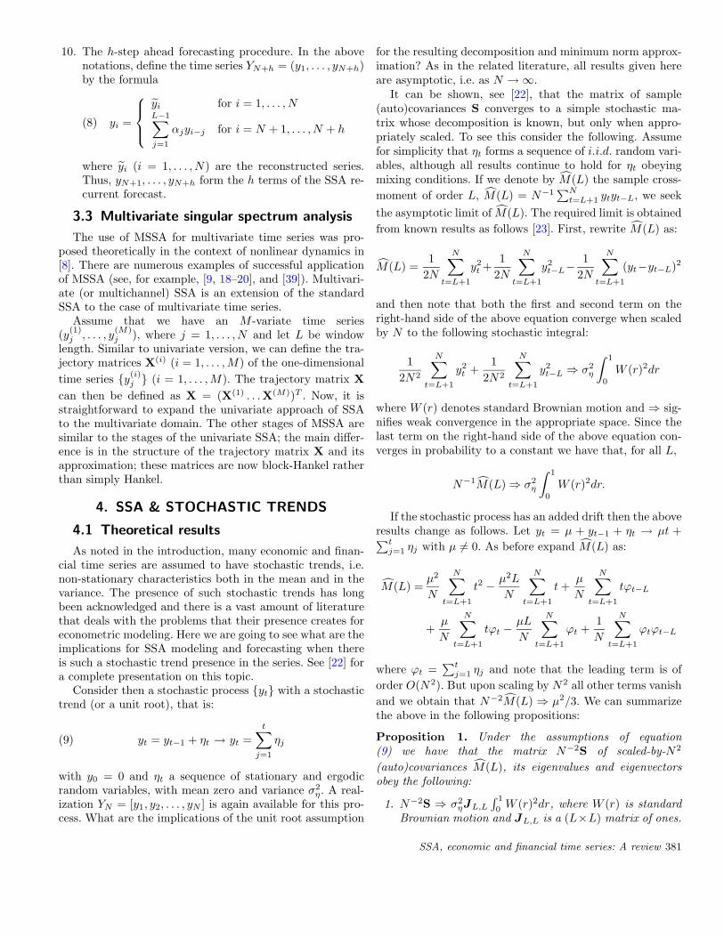
Figure 1 illustrates the above using a sample realizationfrom equation (12) with both εt and ηt being normally dis-tributed and q = 1%, the noise variance being 100 timesgreater than the signal variance, and with L =

√N as be-

fore. The lower panel of the figure shows the true signaland the two smoothed series, the one based on SSA andthe other on the application of fixed point smoothing (withthe parameters estimated). It is clear from the figure thatthe non-parametric SSA smoother performs on par with theparametric fixed point smoother. We further explore theperformance of the proposed methodology in the contextof signal extraction in the simulation section.

In the signal extraction framework one can accommodatea comparison between the SSA method and the Hodrick-Prescott [28] HP-filter that is used frequently in trend ex-traction and smoothing in economics. It can be shown, seefor example [42] and [43], that the HP filter can be derivedfrom a signal extraction model similar to equation (12), butthe signal process yt has two instead of one unit roots, i.e.(1 − B)2yt = ηt, with B being the backshift operator. Thefiltered values can be computed using exactly the same for-mula as in equation (15) before, with Δ being defined as(N × N − 2) with −2 on its principal diagonal and 1’s onthe first upper and lower diagonals. Several methods havebeen proposed in [42] and [43] to consistently estimate σ2

η,σ2

ε and q from the data.

Figure 1. Sample realization from a local level model, signaland smooth series.

4.3 Cointegration & other developments

A natural extension of the material in the previous sec-tions is to consider multiple series with stochastic trendsand perform MSSA on them. This has not been extensivelyconsidered, although [22] has provided a thorough treatmentof the bivariate case that includes SSA-based estimation ofthe cointegration coefficient and SSA-based smoothing ofthe common stochastic trends. There is, however, room foradditional work on this topic using MSSA techniques.

Furthermore, one can define and use a number of relatedpredictors for the reconstructed component of the leadingeigenvalue, for both the univariate case and the multivariatecase. For the univariate case in particular, it can be shownthat the predictor of the smoothed reconstructed componentcoincides with a simple backward moving average — this isuseful as it fully justifies (on SSA grounds) the use of movingaverages as trend predictors in financial time series.

Finally, in related work by Thomakos [24] the problemof SSA-based smoothing of the m-period differences from aprocess with a stochastic trend is studied extensively. Thatis, one considers the differences yt − yt−m of the model inequation (9). This is a non-trivial exercise with theoreti-cal and practical significance. In the theoretical front it isshown that SSA applied to these differences coincides witha version of the discrete cosine transform. In the practicalfront, we have that such differences appear all the time inempirical analysis of economic and financial time series: forexample, annual inflation is defined as the 12-month differ-ence of the (log of) monthly prices; or, consider overlapping

SSA, economic and financial time series: A review 383

multiperiod returns of a financial asset that are obtained bysuch differencing as monthly (20-day) returns obtained bydifferencing of daily prices.

5. SSA-BASED CAUSALITY TESTS

A question that frequently arises in time series analysisis whether one economic variable can help in predicting an-other economic variable. One way to address this questionwas proposed by Granger in [44] where he formalized thecausality concept as follows: process X does not cause pro-cess Y if (and only if) the capability to predict the seriesY based on the histories of all observables is unaffected bythe omission of X’s history (see also [45]). Testing causality,in the Granger sense, involves using F -tests to test whetherlagged information on one variable, say X, provides any sta-tistically significant information about another variable, sayY , in the presence of lagged Y . If not, then “Y does notGranger-cause X.”

Criteria for Granger causality typically have been real-ized in the framework of multivariate Gaussian statisticsvia vector autoregressive (VAR) models. It is worth men-tioning that the linear Granger causality is not a causalityin the broad meaning of the word. It just considers linearprediction and time-lagged dependence between two timeseries. The definition of Granger causality does not includea possibility of an instantaneous dependence between thetwo series. It is not rare when instantaneous dependencebetween two time series can be easily revealed, but sincethe causality can go either way, one usually does not testfor instantaneous dependence. In this paper, we introducedseveral criteria based on the SSA technique to test for theinstantaneous causality.

The general aim of the SSA-based causality tests is toassess the degree of association between two arbitrary timeseries (these associations are often called causal relationshipsas they might be caused by the genuine causality) based onthe observation of these time series. We develop new testsand criteria which will be based on the forecasting accuracyand predictability of the direction of change of the SSA tech-nique. For similarity and dissimilarity between SSA basedtests and Granger Causality tests, and empirical results see[18] and [46].

5.1 Causality criteria based on forecastingaccuracy

The first criterion we use here is based on the out-of-sample forecasting, which is very common in the frameworkof Granger causality. The question behind Granger causalityis whether forecasts of one variable can be improved usingthe history of another variable. Here, we compare the fore-casted value obtained by the univariate procedure, SSA, andby the multivariate one, MSSA. If the forecasting errors us-ing MSSA are significantly smaller than the forecasting er-rors of the univariate SSA, we then conclude that there is acasual relationship between these series.

Let us consider in more detail the procedure of construct-ing a vector of forecasting error for an out-of-sample test.In the first step we divide the series XN = (x1, . . . , xN ) intotwo separate subseries XR and XF : XT = (XR, XF ), whereXR = (x1, . . . , xR) and XF = (xR+1, . . . , xN ). The subseriesXR is used in the reconstruction step to provide the noise-free series XR. The noise-free series XR is then used forforecasting the subseries XF with the help of the recursiveh-step ahead forecast with SSA and MSSA. The forecastedpoints XF = (xR+1, . . . , xN ) are then used for computingthe forecasting error, and the vector (xR+2, . . . , xN ) is fore-casted using the new subseries (x1, . . . , xR+1). This proce-dure is continued recursively up to the end of series, yieldingthe series of h-step-ahead forecasts for univariate and mul-tivariate SSA. Therefore, the two vectors of h-step-aheadforecasts obtained can be used in examining the association(or order h) between the two series. Let us now consider aformal procedure of constructing a criterion of SSA causalityof order h between two arbitrary time series.

Let XT = (x1, . . . , xN ) and YT = (y1, . . . , yN ) denote twodifferent time series of length N . Set the window lengths Lcommon for both series. Using the embedding terminology,we construct the trajectory matrices X = [X1, . . . , XK ] andY = [Y1, . . . , YK ] for the series XN and YN .

Consider an arbitrary loss function L. In economet-rics, the loss function L is usually selected as the meansquare error. Let us first assume that the aim is to fore-cast the series XT h-step ahead. Thus, the aim is to min-imize L(XK+h − XK+h), where the vector XK+h is an es-timate, obtained using a forecasting algorithm, of the vec-tor XK+h = (xK+h, . . . , xT+h). The vector XK+h can beforecasted using either univariate SSA or MSSA. Let usfirst consider the univariate approach. Define ΔXK+h

≡L(XK+h−XK+h), where XK+h is obtained using univariateSSA; that is, the estimate XK+h is obtained only from thevectors [X1, . . . , XK ].

Let XN = (x1, . . . , xN ) and YN+d = (y1, . . . , yN+d) de-note two different time series to be considered simultane-ously and consider the same window length L for both se-ries. Here d is an integer, not necessary non-negative. Now,we forecast xN+1, . . . , xN+h using the information providedby the series YN+d and XN . Next, compute the statisticΔXK+h|YK+d

≡ L(XK+h − XK+h), where XK+h is an esti-mate of XK+h obtained using MSSA. This means that wesimultaneously use vectors [X1, . . . , XK ] and [Y1, . . . , YK+d]in forecasting the vector XK+h. Now, define the criterionF

(h,d)X|Y = ΔXK+h|YK+d

/ΔXK+hcorresponding to the h step

ahead forecast of the series XT in the presence of the se-ries YT+d. Note that d is any given integer (even negative).For example, F

(h,0)X|Y means that d = 0 and that we use the

series XN and YN simultaneously (with zero lag). The cri-terion F

(h,0)X|Y can be used in evaluating the instantaneous

causality.If F

(h,d)X|Y is small, then having information obtained from

the series Y helps us to have a better forecast of the series X.

384 H. Hassani and D. Thomakos

This means there is a relationship between series X and Yof order h according to this criterion. In fact, this measureof association shows that there is much more informationabout the future values of series X contained in the bivari-ate time series (X, Y ) than in the series X alone. If F

(h,d)X|Y

is very small, then the predictions using the multivariateversion are much more accurate than the predictions by theunivariate SSA. If F

(h,d)X|Y < 1, then we conclude that the in-

formation provided by the series Y can be regarded as usefulor supportive for forecasting the series X. Alternatively, ifthe values of F

(h,d)X|Y ≥ 1, then either there is no detectable

association between X and Y or the performance of the uni-variate SSA is better than of the MSSA (this may happen,for example, when the series Y has structural breaks misdi-recting the forecasts of X).

To assess which series is more supportive in forecasting,we need to consider another criteria. We obtain F

(h,d)Y |X in a

similar manner. Now, these measures tell us whether usingextra information about time series YN+d (or XN+d) sup-ports XN (or YN ) in h-step forecasting. If F

(h,d)Y |X < F

(h,d)X|Y ,

we then conclude that X is more supportive to Y than Y

to X. Otherwise, if F(h,d)X|Y < F

(h,d)Y |X , we conclude that Y is

more supportive to X than X to Y .Let us now consider a definition for a feedback system ac-

cording to the above criteria. If F(h,d)Y |X < 1 and F

(h,d)X|Y < 1,

we then conclude that there is a feedback between series Xand Y . We shall call it F-feedback (forecasting feedback)which means that the use of a multivariate system improvesthe forecasting for both series. For a F-feedback system, Xand Y are mutually supportive. To check if the discrepancybetween the two forecasting procedures are statistically sig-nificant, one can employ the test performed in [18] and [46].

5.2 Direction of change based criteria

The direction of change criterion shows the proportionof forecasts that correctly predict the direction of the se-ries movement. For the forecasts obtained using only XN

(univariate case), let ZXi take the value 1 if the forecastobservations correctly predicts the direction of change and0 otherwise. Then ZX =

∑ni=1 ZXi/n shows the proportion

of forecasts that correctly predict the direction of the se-ries movement (in forecasting n data points). The Moivre-Laplace central limit theorem implies that, for large sam-ples, the test statistic 2(ZX −0.5)n1/2 is approximately dis-tributed as standard normal. When ZX is significantly largerthan 0.5, then the forecast is said to have the ability to pre-dict the direction of change. Alternatively, if ZX is signifi-cantly smaller than 0.5, the forecast tends to give the wrongdirection of change.

For the multivariate case, let ZX|Y,i takes a value 1 if theforecast series correctly predicts the direction of change ofthe series X having information about the series Y and 0otherwise. Then, we define the following criterion: D

(h,d)X|Y =

ZX/ZX|Y , where h and d have the same interpretation as forF

(h,d)X|Y . The criterion D

(h,d)X|Y characterizes the improvement

we are getting from the information contained in YT+h (orXT+h) for forecasting the direction of change in the h stepahead forecast.

If D(h,d)X|Y < 1, then having information about the series

Y helps us to have a better prediction of the direction ofchange for the series X. Alternatively, if D

(h,d)X|Y > 1, then

the univariate SSA is better than the multivariate version.To find out which series is more supportive in predict-

ing the direction of change, we consider the following cri-terion. We compute D

(h,d)Y |X in a similar manner. Now, if

D(h,d)Y |X < D

(h,d)X|Y , then we conclude that that X is more sup-

portive (with respect to predicting the direction) to Y thanY to X. Similar to the consideration of the forecasting accu-racy criterion, we can define a feedback system based on thecriterion characterizing the predictability of the direction ofchange. To test the significance of the values of D

(h,d)X|Y , we

use the test developed in [18] and [46].

6. SSA BASED ON THE MINIMUMVARIANCE ESTIMATOR

The SSA algorithms that have been considered in litera-ture are based on the standard SVD and the least squares(LS) estimate (see, for example, [7] and references therein).The LS estimator projects the noisy time series onto theperturbed signal (noise + signal) subspace. Therefore, thereconstructed series using LS estimator has the lowest possi-ble (zero) signal distortion and the highest possible residualnoise level. Moreover, the disadvantage of LS is that the per-formance of the LS estimator is crucially dependent on theestimation of the signal rank r. That is, selecting singularvalues in LS is a binary approach. To overcome this prob-lem, Hassani [15] considered an alternative method which isbased on the minimum variance (MV) estimator. The MVestimator is the optimal linear estimator, which gives theminimum total residual power [47, 48].

Consider a noisy vector YN of length N . Consider againthe signal-plus-noise series without any assumptions aboutthe nature of the signal:

(16) YN = XN + EN ;

here XN represents the signal component and EN the noisecomponent and, as before, we can write the correspondingtrajectory matrices as:

(17) Sy = Sx + Se,

The SVD of the matrix Sy can be written as:

(18) Sy = UΣVT = [Ux Ue][

Σx 00 Σe

] [VT

x

VTe

]SSA, economic and financial time series: A review 385

where Ux ∈ RL×r, Σx ∈ R

r×r and Vx ∈ RK×r. We can

also represent SVD of the Hankel matrix of the signal Sx

as:

(19) Sx = [Ux Ux][

Σx 00 0

] [VT

x

VTx

]It is clear that the Hankel matrix Sx can not be recon-

structed exactly if it is perturbed by noise. To remove theeffect of the noise term, we assume that the vector spaceof the noisy time series (signal) can be split in mutuallyorthogonal noise and signal + noise subspaces. The compo-nents in the noise subspace are suppressed or even removedcompletely. Therefore, one can reconstruct the noise freeseries from signal+noise subspace by choosing the weight.Thus, by adapting the weights of the different singular com-ponents, an estimate of the Hankel matrix Sx, which corre-sponds to a noise-reduced series, can be achieved:

(20) Sx = U(WΣ)VT ,

where W is the diagonal matrix containing the weights.Now, the problem is choosing the weight matrix W.

Let us now consider the weight matrix W based on theLS and MV estimates. The LS and MV estimates can bedefined based on the weight matrix Wr×r as follows:

SxLS = Ux(WLSΣx)VTx(21)

SxMV = Ux(WMV Σx)VTx

where

WLS = Ir×r(22)WMV = diag

((1 − σ2

noise

λ21

), . . . ,

(1 − σ2

noise

λ2r

))7. SSA BASED ON THE PERTURBATION

THEORY

As appears from LS and MV estimate, the singular valuesare different, but the left and right singular vector of the LSand MV estimates are the same and both contain noise term.It is clear that we can obtain a better reconstructed series ifwe remove the noise term from these matrices. Let us definethe following matrices:

Ux = Ux + δUx

Vx = Vx + δVx(23)

Σx = Σx + δΣx

Therefore, the ideal situation is that we remove the noiseterms δUx, δΣx, and δVx. Note that in minimum varianceestimator, we tried to remove δΣx, and in basic SSA wekept all these noisy terms in SVD expansion. An approxi-mation of Ux, Σx and Vx, up to second order perturbation

Table 1. Matrices GU , GΣ and GV for different estimator

Estimation Method GU GΣ GV

Least Square I I IMinimum Variance I WMV I

Perturbation Theory PU PΣ PV

theorem, has been introduced in [16]. We do not provide themathematical formula here and refer the interested readerto [16]. In general, an estimation of signal matrix can berepresented as follows:

(24) Sx = (GUUx)(GΣΣx)(GV VTx )

where matrices GU , GΣ and GV , based on the least square,minimum variance and perturbation theory, are representedin Table 1 where I is an identity matrix, WMV was intro-duced in (22), and matrices PU , PΣ and PV are obtainedup to second order perturbation theory.

Let us now examine the capability of the SSA techniquebased on the perturbation theory (SSAPT ), in reconstruct-ing and forecasting simple simulated sinusoidal series:

S012 = β0 + β1Y1 + β2Y2 + β3Y3 + εt

S01 = β0 + β1Y1 + β2Y2 + εt(25)

S1 = β1Y1 + β2Y2 + εt

where Y1 = Sin(2tπ/12), Y2 = Sin(2tπ/7), Y3 =Sin(2tπ/5), and εt is a white noise series. In total 300 datawere generated and we added different normally distributednoise to each point of the original series. The simulationwas repeated 1,000 times. Note that usually every harmoniccomponent with a different frequency produces two eigen-triples with close singular values (except for frequency 0.5which provides one eigentriples with saw-tooth singular vec-tor). For example, one needs to select the first five eigenval-ues for reconstruction of the series S012, and the first threefor the series S01. It should be noted that we need to con-sider one eigentriple for the intercept, which is the first onein this particular example. To calculate the precision we usethe ratio of Root Mean Square Error (RRMSE): Note that,if RRMSE < 1, then SSAPT procedure outperforms alter-native prediction method. Alternatively, RRMSE > 1 wouldindicate that the performance of the corresponding SSAPT

procedure is worse than the predictions of the competingmethod.

Let us now consider the effect of noise reduction with re-spect to different window length L which is the single param-eter in decomposition stage. Certainly, the improper choiceof L would imply an inferior decomposition. It should benoted that variations in L may influence the separability fea-tures when applying SSA, specifically the orthogonality and

386 H. Hassani and D. Thomakos

Figure 2. The value of RRMSE in reconstructing of noisyseries S012 for different window length.

Figure 3. The value of RRMSE in reconstructing of noisyseries S01 for different window length.

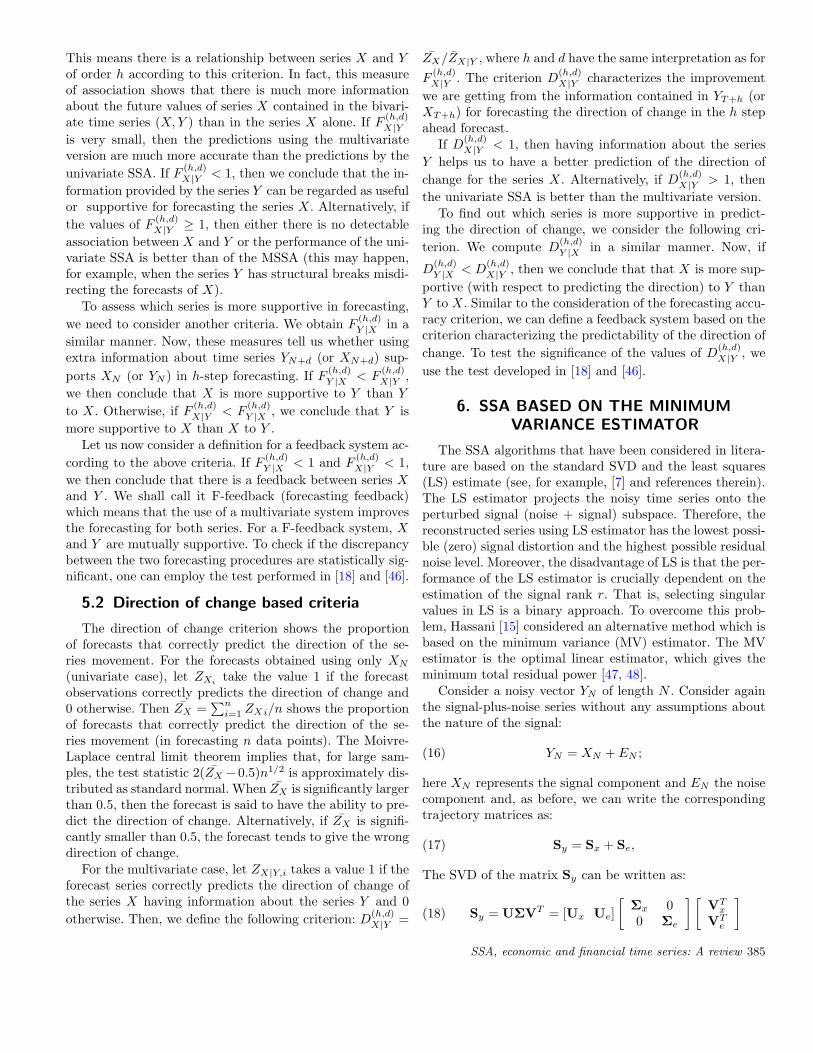
closeness of the singular values. Here we consider L between10 and 70 which is approximately N/3 (here N = 200).

Figures 2–4 show the RRMSE of reconstructed series fordifferent simulated series. As it appears from these figures,SSAPT has a better performance in reconstruction noisyseries, particulary for small window length. The performanceof both methods are similar for a large window length.

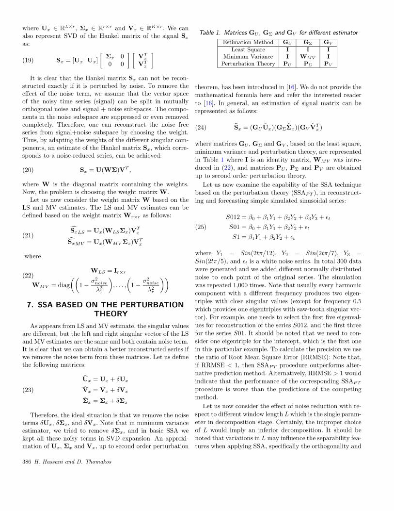
As the figures show, RRMSE tends to 1 as the windowlength increases confirming that both methods have simi-lar performance for a large window length. The graphs alsoshow that there is a gradual increase in RRMSE with win-dow length. For example for window length 10, the perfor-mance of SSAPT is up to 15% better than SSALS in recon-struction noisy series S01. However, there is not a significantdiscrepancy between the performance of SSAPT and SSALS

for window length greater than 50.Note that the minimum value of RMSE for both SSAPT

and SSALS occurs for a large window length. Let us, forexample, consider the RMSE of SSAPT and SSALS in re-constructing S012 in more detail. Figure 5 shows the RMSE

Figure 4. The value of RRMSE in reconstructing of noisyseries S1 for different window length.

Figure 5. The value of RMSE in reconstructing of noisy sinfor different window length using SSAPT (dashed line) and

SSALS (thick line).

of SSAPT and SSALS . As it can be seen from the figure,there is a gradual decrease in RMSE with window length.In fact, the maximum accuracy in reconstruction, using bothmethods, occurs for a large window length. The figure alsoshows that the RMSE of SSAPT is smaller than those ob-tained using SSALS . Moreover, the figure indicates that thediscrepancy between SSAPT and SSALS reduces as windowlength increases.

8. SMOOTHING & SIGNAL EXTRACTION

8.1 Simulations results

In this section we present some simulation results on theperformance of the SSA-based smoother in the context ofthe signal extraction problem. The data generating processis the local level model of equation (12) with different valuesfor the signal-to-noise ratio q and different assumptions onthe distribution of ηt. For a sample size of N = 250 observa-

SSA, economic and financial time series: A review 387

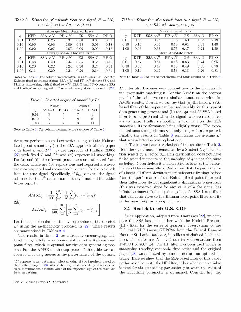
Table 2. Dispersion of residuals from true signal, N = 250,εt ∼ K(0, σ2

ε ) and ηt ∼ K(0, σ2η)

Average Mean Squared Error

q KFP SSA-√

N PP-√

N ES SSA-O PP-O0.01 0.22 0.25 0.31 0.50 0.80 0.320.10 0.06 0.08 0.09 0.15 0.09 0.181.00 0.02 0.07 0.07 0.06 0.03 0.17

Average Mean Absolute Error

q KFP SSA-√

N PP-√

N ES SSA-O PP-O0.01 0.38 0.40 0.44 0.55 0.68 0.450.10 0.20 0.22 0.24 0.30 0.24 0.331.00 0.11 0.20 0.21 0.20 0.14 0.31

Notes to Table 2. The column nomenclature is as follows: KFP denotesKalman fixed point smoothing; SSA-

√N and PP-

√N denote SSA and

Phillips’ smoothing with L fixed to√

N ; SSA-O and PP-O denote SSAand Phillips’ smoothing with L∗ selected via equation proposed in [22].

Table 3. Selected degree of smoothing L∗

N=250 N=500q SSA-O PP-O SSA-O PP-O

0.01 6 7 7 90.10 6 7 8 101.00 6 8 8 11

Note to Table 3. For column nomenclature see note of Table 2.

tions, we perform a signal extraction using: (a) the Kalmanfixed point smoother; (b) the SSA approach of this paperwith fixed L and L∗2; (c) the approach of Phillips (2005)[27] with fixed L and L∗; and (d) exponential smoothing.For (a) and (d) the relevant parameters are estimated fromthe data. There are 500 replications and reported are aver-age mean-squared and mean-absolute errors for the residualsfrom the true signal. Specifically, if yt,ij denotes the signalestimate for the ith replication for the jth method the tablesbelow report:

AMSEj =1

500

500∑i=1

[1N

N∑t=1

(yt,i − yt,ij)2]

,

(26)

AMAEj =1

500

500∑i=1

[1N

N∑t=1

|yt,i − yt,ij |]

For the same simulations the average value of the selectedL∗ using the methodology proposed in [22]. These resultsare summarized in Tables 2–4.

The results in Table 2 are extremely encouraging. Thefixed L =

√N filter is very competitive to the Kalman fixed

point filter, which is optimal for the data generating pro-cess. For the AMSE on the top panel of the table we canobserve that as q increases the performance of the optimal2L∗ represents an ‘optimally’ selected value of the threshold based onthe methodology in [38] where the degree of smoothing is selected soas to minimize the absolute value of the expected sign of the residualsfrom smoothing.

Table 4. Dispersion of residuals from true signal, N = 250,εt ∼ K(0, σ2

ε ) and ηt ∼ t(2)ση

Mean Squared Error

q KFP SSA-√

N PP-√

N ES SSA-O PP-O0.01 0.58 0.93 1.13 1.50 1.03 2.180.10 0.16 0.63 0.68 0.61 0.31 1.401.00 0.03 0.68 0.75 0.47 0.24 1.59

Mean Absolute Error

q KFP SSA-√

N PP-√

N ES SSA-O PP-O0.01 0.57 0.61 0.68 0.83 0.74 0.950.10 0.30 0.49 0.53 0.49 0.35 0.781.00 0.14 0.49 0.53 0.33 0.26 0.81

Note to Table 4. Column nomenclature and table entries as in Table 2.

L∗ filter also becomes very competitive to the Kalman fil-ter, eventually matching it. For the AMAE on the bottompanel of the table we see a similar situation as with theAMSE results. Overall we can say that (a) the fixed L SSA-based filter of this paper can be used reliably for this type ofdata generating process; and (b) the optimal L∗ SSA-basedfilter is to be preferred when the signal-to-noise ratio is rel-atively large. Phillip’s smoother is trailing after the SSAsmoother, its performance being slightly worse. The expo-nential smoother performs well only for q = 1, as expected.Finally, the results in Table 3 summarize the average L∗

that was selected across replications.In Table 4 we have a variation of the results in Table 2.

Here the signal noise is generated by a Student t(2) distribu-tion scaled by a factor ση. This distribution does not havefinite second moments so the meaning of q is not the sameas before. Nevertheless it is instructive to look at the perfor-mance of the various filters. We can see that the performanceof almost all filters deviates more substantially than beforefrom the performance of the Kalman fixed point filter andtheir differences do not significantly diminish as q increases(this was expected since for any value of q the signal hasinfinite variance). It is only the optimal L∗ SSA-based filterthat can come close to the Kalman fixed point filter and itsperformance improves as q increases.

8.2 Real data set: U.S. GDP

As an application, adapted from Thomakos [22], we com-pare the SSA-based smoother with the Hodrick-Prescott(HP) filter for the series of quarterly observations of theU.S. real GDP (series GDPC96 from the Federal ReserveBank of St. Louis Database, in billions of chained 2,000 dol-lars). The series has N = 244 quarterly observations from1947:Q1 to 2007:Q4. The HP filter has been used widely insmoothing trending economic time series and the originalpaper [28] was followed by much literature on optimal fil-tering. Here we show that the SSA-based filter of this paperperforms on par with the HP filter, either when a naive valueis used for the smoothing parameter q or when the value ofthe smoothing parameter is optimized. Consider first the

388 H. Hassani and D. Thomakos

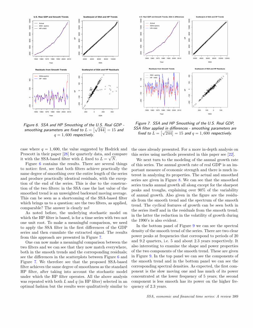
Figure 6. SSA and HP Smoothing of the U.S. Real GDP -smoothing parameters are fixed to L =

[√244]

= 15 andq = 1, 600 respectively.

case where q = 1, 600, the value suggested by Hodrick andPrescott in their paper [28] for quarterly data, and compareit with the SSA-based filter with L fixed to L =

√N .

Figure 6 contains the results. There are several thingsto notice: first, see that both filters achieve practically thesame degree of smoothing over the entire length of the seriesand produce practically identical residuals, with the excep-tion of the end of the series. This is due to the construc-tion of the two filters: in the SSA case the last value of thesmoothed trend is an unweighted backward moving average.This can be seen as a shortcoming of the SSA-based filterwhich brings us to a question: are the two filters, as applied,comparable? The answer is clearly no!

As noted before, the underlying stochastic model onwhich the HP filter is based, is for a time series with two notone unit root. To make a meaningful comparison, we needto apply the SSA filter in the first differences of the GDPseries and then cumulate the extracted signal. The resultsfrom this approach are presented in Figure 7.

One can now make a meaningful comparison between thetwo filters and we can see that they now match everywhere,both in the smooth trends and the corresponding residuals;see the differences in the scatterplots between Figure 6 andFigure 7. We therefore see that the proposed SSA-basedfilter achieves the same degree of smoothness as the standardHP filter, after taking into account the stochastic modelunder which the HP filter operates. All the above analysiswas repeated with both L and q (in HP filter) selected in anoptimal fashion but the results were qualitatively similar to

Figure 7. SSA and HP Smoothing of the U.S. Real GDP,SSA filter applied in differences - smoothing parameters are

fixed to L =[√

244]

= 15 and q = 1, 600 respectively.

the ones already presented. For a more in-depth analysis onthis series using methods presented in this paper see [22].

We next turn to the modeling of the annual growth rateof this series. The annual growth rate of real GDP is an im-portant measure of economic strength and there is much in-terest in analyzing its properties. The actual and smoothedseries are given in Figure 8. We can see that the smoothedseries tracks annual growth all along except for the sharpestpeaks and troughs, explaining over 90% of the variabilityof annual growth. Also given in the figure are the residu-als from the smooth trend and the spectrum of the smoothtrend. The cyclical features of growth can be seen both inthe series itself and in the residuals from the smooth trend;in the latter the reduction in the volatility of growth duringthe 1990’s is also evident.

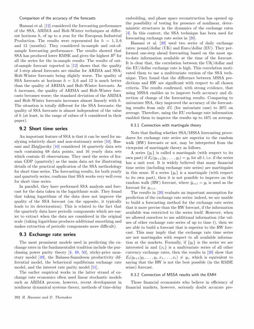
In the bottom panel of Figure 9 we can see the spectraldensity of the smooth trend of the series. There are two clearpower peaks at frequencies that correspond to periods of 20and 9.2 quarters, i.e. 5 and about 2.3 years respectively. Italso interesting to examine the shape and power propertiesof the two components of the smooth trend. These are givenin Figure 9. In the top panel we can see the components ofthe smooth trend and in the bottom panel we can see thecorresponding spectral densities. As expected, the first com-ponent is the slow moving one and has much of its powerconcentrated at the lower frequency of 5 years; the secondcomponent is less smooth has its power on the higher fre-quency of 2.3 years.

SSA, economic and financial time series: A review 389

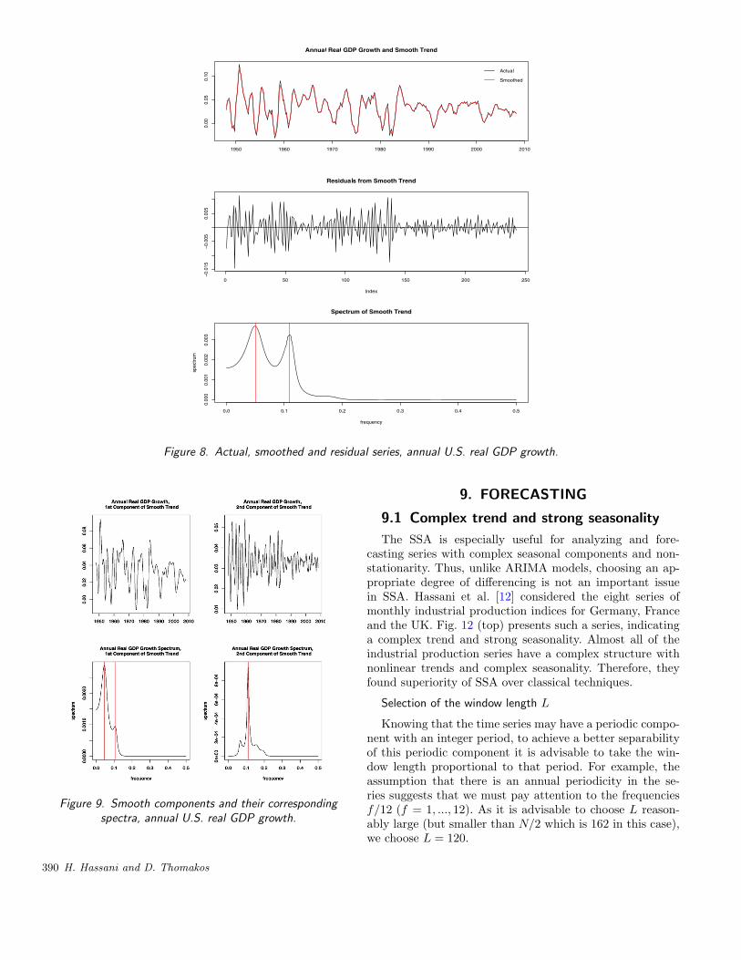
Figure 8. Actual, smoothed and residual series, annual U.S. real GDP growth.

Figure 9. Smooth components and their correspondingspectra, annual U.S. real GDP growth.

9. FORECASTING

9.1 Complex trend and strong seasonality

The SSA is especially useful for analyzing and fore-casting series with complex seasonal components and non-stationarity. Thus, unlike ARIMA models, choosing an ap-propriate degree of differencing is not an important issuein SSA. Hassani et al. [12] considered the eight series ofmonthly industrial production indices for Germany, Franceand the UK. Fig. 12 (top) presents such a series, indicatinga complex trend and strong seasonality. Almost all of theindustrial production series have a complex structure withnonlinear trends and complex seasonality. Therefore, theyfound superiority of SSA over classical techniques.

Selection of the window length L

Knowing that the time series may have a periodic compo-nent with an integer period, to achieve a better separabilityof this periodic component it is advisable to take the win-dow length proportional to that period. For example, theassumption that there is an annual periodicity in the se-ries suggests that we must pay attention to the frequenciesf/12 (f = 1, ..., 12). As it is advisable to choose L reason-ably large (but smaller than N/2 which is 162 in this case),we choose L = 120.

390 H. Hassani and D. Thomakos

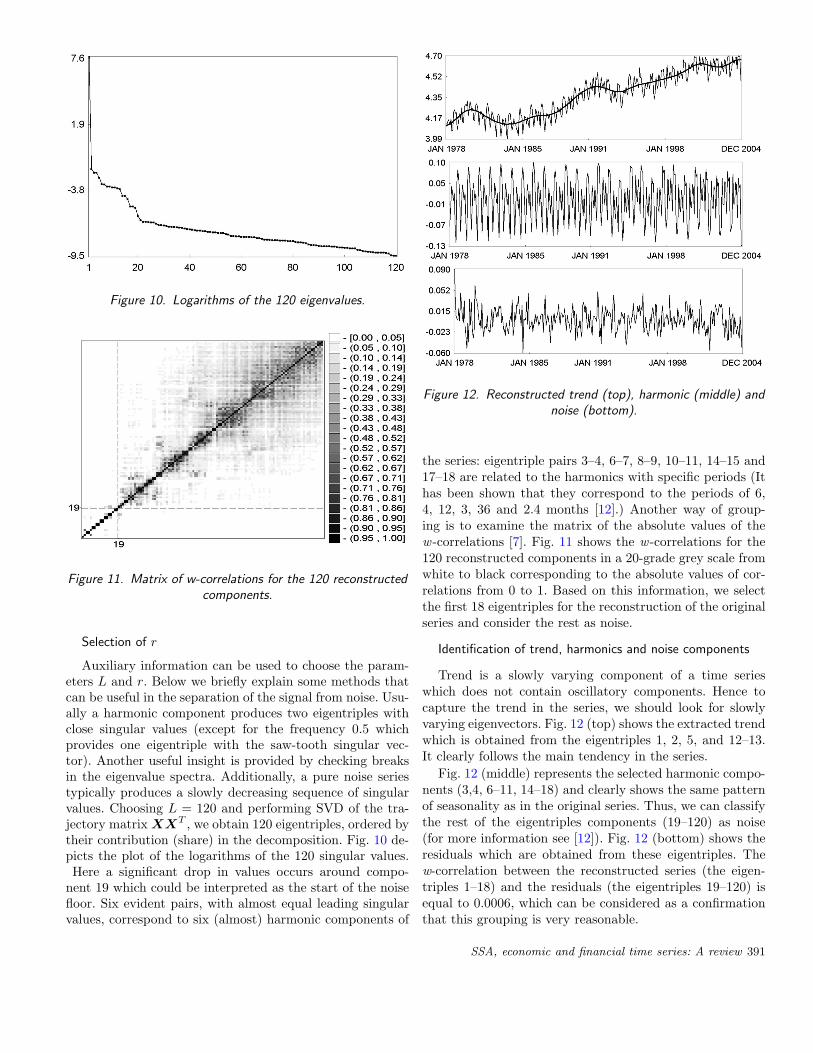
Figure 10. Logarithms of the 120 eigenvalues.

Figure 11. Matrix of w-correlations for the 120 reconstructedcomponents.

Selection of r

Auxiliary information can be used to choose the param-eters L and r. Below we briefly explain some methods thatcan be useful in the separation of the signal from noise. Usu-ally a harmonic component produces two eigentriples withclose singular values (except for the frequency 0.5 whichprovides one eigentriple with the saw-tooth singular vec-tor). Another useful insight is provided by checking breaksin the eigenvalue spectra. Additionally, a pure noise seriestypically produces a slowly decreasing sequence of singularvalues. Choosing L = 120 and performing SVD of the tra-jectory matrix XXT , we obtain 120 eigentriples, ordered bytheir contribution (share) in the decomposition. Fig. 10 de-picts the plot of the logarithms of the 120 singular values.Here a significant drop in values occurs around compo-

nent 19 which could be interpreted as the start of the noisefloor. Six evident pairs, with almost equal leading singularvalues, correspond to six (almost) harmonic components of

Figure 12. Reconstructed trend (top), harmonic (middle) andnoise (bottom).

the series: eigentriple pairs 3–4, 6–7, 8–9, 10–11, 14–15 and17–18 are related to the harmonics with specific periods (Ithas been shown that they correspond to the periods of 6,4, 12, 3, 36 and 2.4 months [12].) Another way of group-ing is to examine the matrix of the absolute values of thew -correlations [7]. Fig. 11 shows the w -correlations for the120 reconstructed components in a 20-grade grey scale fromwhite to black corresponding to the absolute values of cor-relations from 0 to 1. Based on this information, we selectthe first 18 eigentriples for the reconstruction of the originalseries and consider the rest as noise.

Identification of trend, harmonics and noise components

Trend is a slowly varying component of a time serieswhich does not contain oscillatory components. Hence tocapture the trend in the series, we should look for slowlyvarying eigenvectors. Fig. 12 (top) shows the extracted trendwhich is obtained from the eigentriples 1, 2, 5, and 12–13.It clearly follows the main tendency in the series.

Fig. 12 (middle) represents the selected harmonic compo-nents (3,4, 6–11, 14–18) and clearly shows the same patternof seasonality as in the original series. Thus, we can classifythe rest of the eigentriples components (19–120) as noise(for more information see [12]). Fig. 12 (bottom) shows theresiduals which are obtained from these eigentriples. Thew-correlation between the reconstructed series (the eigen-triples 1–18) and the residuals (the eigentriples 19–120) isequal to 0.0006, which can be considered as a confirmationthat this grouping is very reasonable.

SSA, economic and financial time series: A review 391

Comparison of the accuracy of the forecasts

Hassani et al. [12] considered the forecasting performanceof the SSA, ARIMA and Holt-Winter techniques at differ-ent horizons h, of up to a year for the European IndustrialProduction. The results were represented for h = 1, 3, 6and 12 (months). They considered in-sample and out-of-sample forecasting performance. The results showed thatSSA has produced lower RMSE and gives the highest R2 forall the series for the in-sample results. The results of out-of-sample forecast reported in [12] shows that the qualityof 1-step ahead forecasts are similar for ARIMA and SSA;Holt-Winter forecasts being slightly worse. The quality ofSSA forecasts at horizons h = 3, 6 and 12 is much betterthan the quality of ARIMA and Holt-Winter forecasts. Ash increases, the quality of ARIMA and Holt-Winter fore-casts becomes worse; the standard deviation of the ARIMAand Holt-Winter forecasts increases almost linearly with h.The situation is totally different for the SSA forecasts: thequality of SSA forecasts is almost independent of the valueof h (at least, in the range of values of h considered in theirpaper).

9.2 Short time series

An important feature of SSA is that it can be used for an-alyzing relatively short and non-stationary series [10]. Has-sani and Zhigljavsky [10] considered 16 quarterly data setseach containing 68 data points, and 16 yearly data setswhich contain 45 observations. They used the series of Ira-nian GDP (quarterly) as the main data set for illustratingdetails of the practical application of the SSA methodologyfor short time series. The forecasting results, for both yearlyand quarterly series, confirms that SSA works very well evenfor short time series.

In parallel, they have performed SSA analysis and fore-cast for the data taken in the logarithmic scale. They foundthat taking logarithms of the data does not improve thequality of the SSA forecast (on the opposite, it typicallyleads to its deterioration). This is related to the fact thatthe quarterly data have periodic components which are eas-ier to extract when the data are considered in the originalscale (taking logarithms produces additional smoothing andmakes extraction of periodic components more difficult).

9.3 Exchange rate series

The most prominent models used in predicting the ex-change rates in the fundamentalist tradition include the pur-chasing power parity theory [4, 49, 50], sticky-price mon-etary model [49], the Balassa-Samuleson productivity dif-ferential model, the behavioral equilibrium exchange ratemodel, and the interest rate parity model [51].

The earlier empirical works in the latter strand of ex-change rate economics often used linear stochastic modelssuch as ARIMA process, however, recent development innonlinear dynamical systems theory, methods of time-delay

embedding, and phase space reconstruction has opened upthe possibility of testing for presence of nonlinear, deter-ministic structures in the dynamics of the exchange rates[4]. In this context, the SSA technique has been used forforecasting exchange rate series in [20].

Hassani et al. [20] used two series of daily exchangerates: pound/dollar (UK) and Euro/dollar (EU). They per-formed one-step ahead forecasting based on the most up-to-date information available at the time of the forecast.It is clear that, the correlation between the UK/dollar andthe EU/dollar exchange rate is high. This correlation moti-vated them to use a multivariate version of the SSA tech-nique. They found that the difference between MSSA pre-dictions and RW are significant with respect to all chosencriteria. The results confirmed, with strong evidence, thatusing MSSA enables us to improve both accuracy and di-rection of change of the forecasting results. Comparing tounivariate SSA, they improved the accuracy of the forecast-ing results from only 4% (for univariate case) to 20% onaverage. Therefore, using the EU exchange rate informationenabled them to improve the results up to 16% on average.

9.3.1 Connection with martingale theory

Note that finding whether SSA/MSSA forecasting proce-dures for exchange rate series are superior to the randomwalk (RW) forecasts or not, may be interpreted from theviewpoint of martingale theory as follows.

A series {yt} is called a martingale (with respect to itsown past) if Et(yt+1|y1, . . . , yt) = yt for all t, i.e. if the serieshas a unit root. It is widely believed that many financialtime series (including exchange rate series) are martingalesin this sense. If a series {yt} is a martingale (with respectto its own past), then it is not possible to improve on therandom walk (RW) forecast, where yt+1 = yt is used as theforecast for yt+1.

The results in [20] evaluate an important assumption forprediction of the exchange rate series: indeed, we are unableto build a forecasting method for the exchange rate seriesthat is more precise than the RW forecast, if the informationavailable was restricted to the series itself. However, whenwe allowed ourselves to use additional information (the val-ues of other exchange rate series of up to time t), then weare able to build a forecast that is superior to the RW fore-cast. This may imply that the exchange rate time seriesare not martingales with respect to all available informa-tion at the markets. Formally, if {yt} is the series we areinterested in and {xt} is a multivariate series of all othercurrency exchange rates, then the results in [20] show thatEt(yt+1|y1, . . . , yt, x1, . . . , xt) �= yt, which is equivalent tosaying that the RW is not the best possible (in the RMSEsense) forecast.

9.3.2 Connection of MSSA results with the EMH

Those financial economists who believe in efficiency offinancial markets, however, seriously doubt accurate pre-

392 H. Hassani and D. Thomakos

dictability of the financial asset prices. Efficient Market Hy-pothesis (EMH) in its weak form implies that the returns offinancial asset prices are white noise processes consisting ofindependent, identically distributed random variables. Thewhite noise nature of the returns implies that the series atlevel follows a random walk model and is unpredictable.

In spite of the popularity of EMH, mostly in the aca-demic circles, a vast literature dealing with predictions ofthe financial asset prices exists. Reviewing the empiricalexchange rate economics literature one could discern twostrands of research in the field that closely follow fundamen-talist and chartist (technical analyst and its rough coun-terpart in academia time series analysts) that prevails inprediction of equity prices in the stock markets. In the con-text of exchange rate economics, the fundamentalists believethat the money supply, the price level, national income, in-terest rates, productivity, and other relevant economic vari-ables determine exchange rates. The empirical results of thepresent study are instructive in examining the efficient mar-ket hypothesis controversy. Accordingly, we first present for-mal discussions of the martingale games, random walk pro-cesses, their relationship with the EMH, and then we elab-orate on the implications of our findings for the EMH.

A stochastic process xt follows a martingale if

(27) Et(yt+1|Ωt) = yt

where Ωt is the information set at time t that includes yt

also. Equation (27) implies that if yt follows a martingalethe best forecast of yt+1 is yt, given the information set Ωt.

The implication of the fair game model (27) in financialeconomics is that the returns of the asset price yt are un-predictable, given the information set Ωt. Accordingly, theinformation set Ωt is fully reflected in the asset price, andthis is known as the EMH3.

Note that one may restrict the information set Ωt only tothe asset’s past price history, making alternative represen-tation of (27) as

(28) E(yt+1|yt, yt−1, . . .) = yt

What are the implications of the MSSA forecasting re-sults for the EMH? Based on the results of random walkpredictions, which are based only on the past price his-tory, we conclude that the currency markets are efficient.However, the results based on MSSA which are obtained byincluding other information, i.e. EU/dollar exchange rate,clearly point to inadequacy of the random walk in modelingexchange rate for predictions. Moreover, the superior resultsobtained from the direction of change criterion, also provideadditional support for the view that currency markets maynot be efficient in the sense discussed above (for further in-formation see [20]).3We are using EMH in a generic sense, to avoid further discussion ofthe types of efficient market hypothesis which is not germane to theissue here.

9.4 Inflation rate series

In recent years a number of comparative studies of in-flation forecasting methods resulted in two major insightsabout inflation forecasting methods and inflation rate inthe United States. First, the studies are inconclusive aboutthe superiority of the competing forecasting methods. Forexample, Stock and Watson [52] documents that Phillipscurve-based models tend to have the most accurate fore-cast of the inflation in the United States up to 1996. WhileAtkeson and Ohanian [53] contradicts the conclusion aboutthe relative forecasting accuracy of the Phillips curve-basedmodels and shows that a naive random walk model has asuperior predictive capability. Given that the dynamics ofthe U.S. economy has gone through many variations due topolicy and structural changes during the time period underconsideration, one needs to make certain that the methodof prediction is not sensitive to the dynamical variations.Therefore, SSA can be considered as a suitable techniquefor the forecasting US inflation rate.

9.4.1 Forecasting US inflation rate based on the CPI-all andCPI-core series

Let us now consider several U.S. price indexes in out-of-sample, h-step-ahead moving prediction exercises. Theseindices including consumer price index with and withouthighly volatile food and energy items, CPI-all and CPI-core,respectively as well as real-time quarterly chain-weightedGDP price index. Specifically, we used monthly CPI-all andCPI-core data for the period JAN 1986 – DEC 2006. Wedo not report inflation forecasting based on GDP price in-dex here (the results can be found in [16]). We use movingh-step-ahead prediction, which means that we include allavailable information for the predictions.

The MSSA has been used for forecasting inflation ratebased on the CPI-all and CPI-core series over the periodJan-1986 to Dec-1996 that was used as the training set data[16]. The forecasting results indicate that MSSA outper-forms the random walk predictions in both one and 3-stepahead forecasts. Additionally, the test results for the nullhypothesis of whether the percentages of the direction ofchanges are greater than the pure chance (50%) shows thatall results are statistically significant and higher than a 50%chance. The important result is that MSSA predicts direc-tion of change for 3-step as accurately as it can predict 1-step ahead. This confirms that we are able to capture thehidden dynamic in the inflation series using MSSA which isnot usually captured by other classical methods. The resultsobtained below can be considered as a confirmation for thisconclusion.

9.4.2 Comparison with the other methods

Comparative study is somewhat difficult, since data,methods, forecasting horizons and error criteria are not uni-

SSA, economic and financial time series: A review 393

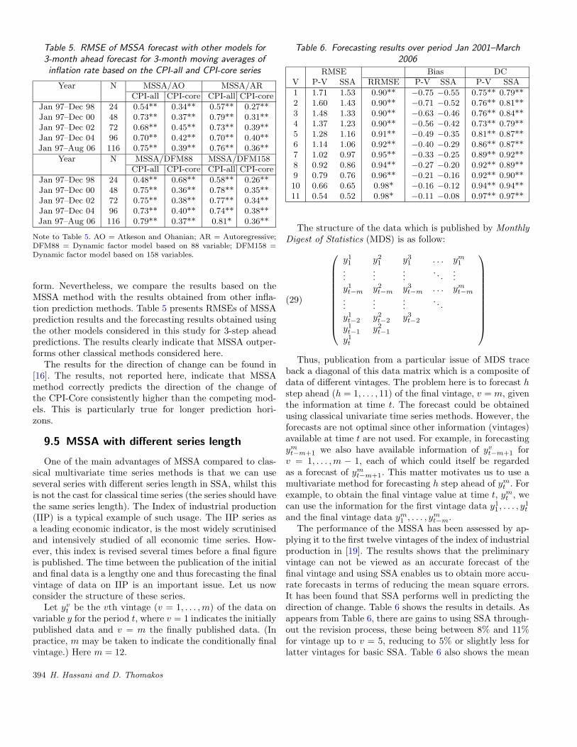
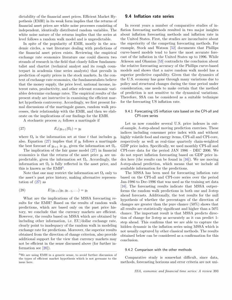
Table 5. RMSE of MSSA forecast with other models for3-month ahead forecast for 3-month moving averages ofinflation rate based on the CPI-all and CPI-core series

Year N MSSA/AO MSSA/ARCPI-all CPI-core CPI-all CPI-core

Jan 97–Dec 98 24 0.54** 0.34** 0.57** 0.27**Jan 97–Dec 00 48 0.73** 0.37** 0.79** 0.31**Jan 97–Dec 02 72 0.68** 0.45** 0.73** 0.39**Jan 97–Dec 04 96 0.70** 0.42** 0.70** 0.40**Jan 97–Aug 06 116 0.75** 0.39** 0.76** 0.36**

Year N MSSA/DFM88 MSSA/DFM158CPI-all CPI-core CPI-all CPI-core

Jan 97–Dec 98 24 0.48** 0.68** 0.58** 0.26**Jan 97–Dec 00 48 0.75** 0.36** 0.78** 0.35**Jan 97–Dec 02 72 0.75** 0.38** 0.77** 0.34**Jan 97–Dec 04 96 0.73** 0.40** 0.74** 0.38**Jan 97–Aug 06 116 0.79** 0.37** 0.81* 0.36**

Note to Table 5. AO = Atkeson and Ohanian; AR = Autoregressive;DFM88 = Dynamic factor model based on 88 variable; DFM158 =Dynamic factor model based on 158 variables.

form. Nevertheless, we compare the results based on theMSSA method with the results obtained from other infla-tion prediction methods. Table 5 presents RMSEs of MSSAprediction results and the forecasting results obtained usingthe other models considered in this study for 3-step aheadpredictions. The results clearly indicate that MSSA outper-forms other classical methods considered here.

The results for the direction of change can be found in[16]. The results, not reported here, indicate that MSSAmethod correctly predicts the direction of the change ofthe CPI-Core consistently higher than the competing mod-els. This is particularly true for longer prediction hori-zons.

9.5 MSSA with different series length

One of the main advantages of MSSA compared to clas-sical multivariate time series methods is that we can useseveral series with different series length in SSA, whilst thisis not the cast for classical time series (the series should havethe same series length). The Index of industrial production(IIP) is a typical example of such usage. The IIP series asa leading economic indicator, is the most widely scrutinisedand intensively studied of all economic time series. How-ever, this index is revised several times before a final figureis published. The time between the publication of the initialand final data is a lengthy one and thus forecasting the finalvintage of data on IIP is an important issue. Let us nowconsider the structure of these series.

Let yvt be the vth vintage (v = 1, . . . ,m) of the data on

variable y for the period t, where v = 1 indicates the initiallypublished data and v = m the finally published data. (Inpractice, m may be taken to indicate the conditionally finalvintage.) Here m = 12.

Table 6. Forecasting results over period Jan 2001–March2006

RMSE Bias DCV P-V SSA RRMSE P-V SSA P-V SSA

1 1.71 1.53 0.90** −0.75 −0.55 0.75** 0.79**2 1.60 1.43 0.90** −0.71 −0.52 0.76** 0.81**3 1.48 1.33 0.90** −0.63 −0.46 0.76** 0.84**4 1.37 1.23 0.90** −0.56 −0.42 0.73** 0.79**5 1.28 1.16 0.91** −0.49 −0.35 0.81** 0.87**6 1.14 1.06 0.92** −0.40 −0.29 0.86** 0.87**7 1.02 0.97 0.95** −0.33 −0.25 0.89** 0.92**8 0.92 0.86 0.94** −0.27 −0.20 0.92** 0.89**9 0.79 0.76 0.96** −0.21 −0.16 0.92** 0.90**10 0.66 0.65 0.98* −0.16 −0.12 0.94** 0.94**11 0.54 0.52 0.98* −0.11 −0.08 0.97** 0.97**

The structure of the data which is published by MonthlyDigest of Statistics (MDS) is as follow:

(29)

⎛⎜⎜⎜⎜⎜⎜⎜⎜⎜⎜⎝

y11 y2

1 y31 . . . ym

1...

......

. . ....

y1t−m y2

t−m y3t−m . . . ym

t−m...

......

. . .y1

t−2 y2t−2 y3

t−2

y1t−1 y2

t−1

y1t

⎞⎟⎟⎟⎟⎟⎟⎟⎟⎟⎟⎠Thus, publication from a particular issue of MDS trace

back a diagonal of this data matrix which is a composite ofdata of different vintages. The problem here is to forecast hstep ahead (h = 1, . . . , 11) of the final vintage, v = m, giventhe information at time t. The forecast could be obtainedusing classical univariate time series methods. However, theforecasts are not optimal since other information (vintages)available at time t are not used. For example, in forecastingym

t−m+1 we also have available information of yvt−m+1 for

v = 1, . . . ,m − 1, each of which could itself be regardedas a forecast of ym

t−m+1. This matter motivates us to use amultivariate method for forecasting h step ahead of ym

t . Forexample, to obtain the final vintage value at time t, ym

t , wecan use the information for the first vintage data y1

1 , . . . , y1t

and the final vintage data ym1 , . . . , ym

t−m.The performance of the MSSA has been assessed by ap-

plying it to the first twelve vintages of the index of industrialproduction in [19]. The results shows that the preliminaryvintage can not be viewed as an accurate forecast of thefinal vintage and using SSA enables us to obtain more accu-rate forecasts in terms of reducing the mean square errors.It has been found that SSA performs well in predicting thedirection of change. Table 6 shows the results in details. Asappears from Table 6, there are gains to using SSA through-out the revision process, these being between 8% and 11%for vintage up to v = 5, reducing to 5% or slightly less forlatter vintages for basic SSA. Table 6 also shows the mean

394 H. Hassani and D. Thomakos

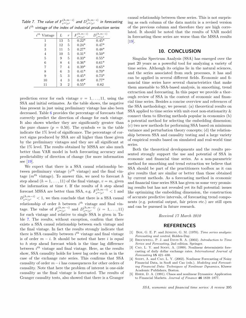
Table 7. The value of F(h,m−i)vm|vi and D

(h,m−i)vm|vi in forecasting

of ith vintage of the index of industrial production series

ith Vintage L r F(h,m−i)

vm|vi D(h,m−i)

vm|vi

1 13 5 0.22* 0.45*2 12 5 0.24* 0.47*3 11 5 0.27* 0.48*4 10 5 0.31* 0.50*5 9 5 0.33* 0.55*6 8 4 0.36* 0.61*7 7 4 0.39* 0.65*8 6 3 0.41* 0.70*9 5 3 0.45* 0.73*10 4 3 0.49* 0.77*11 3 2 0.55* 0.82

prediction error for each vintage v = 1, . . . , 11, using theSSA and initial estimates. As the table shows, the negativebias present in just using preliminary vintage has also beendecreased. Table 6 provides the percentage of forecasts thatcorrectly predict the direction of change for each vintage.It also shows whether they are significantly greater thanthe pure chance (p = 0.50). The symbols ∗∗ in the tableindicate the 1% level of significance. The percentage of cor-rect signs produced by SSA are all higher than those givenby the preliminary vintages and they are all significant atthe 1% level. The results obtained by MSSA are also muchbetter than VAR model in both forecasting accuracy andpredictability of direction of change (for more informationsee [19].

We expect that there is a SSA causal relationship be-tween preliminary vintage (vth vintage) and the final vin-tage (mth vintage). To answer this, we need to forecast hstep ahead (h = 1, . . . , 11) of the final vintage, v = m, giventhe information at time t. If the results of h step aheadforecast MSSA are better than SSA, e.g. F

(h,m−i)vm|vi < 1 and

D(h,m−i)vm|vi < 1, we then conclude that there is a SSA causal

relationship of order h between ith vintage and final vin-tage. The value of F

(h,m−i)vm|vi and D

(h,m−i)vm|vi (i = 1, . . . , 11)

for each vintage and relative to single SSA is given in Ta-ble 7. The results, without exception, confirm that thereexists a SSA causal relationship between each vintage andthe final vintage. In fact the results strongly indicate thatthere is SSA causality between ith vintage and final vintageis of order m − i. It should be noted that here i is equalto h step ahead forecast which is the time lag differencebetween ith vintage and final vintage. Here, as the resultsshow, SSA causality holds for lower lag order such as in thecase of the exchange rate series. This confirms that SSAcausality of order m− i has consequences for other orders ofcausality. Note that here the problem of interest is one-sidecausality as the final vintage is forecasted. The results ofGranger causality tests, also showed that there is a Granger

causal relationship between these series. This is not surpris-ing as each column of the data matrix is a revised versionof the previous column and therefore they are high corre-lated. It should be noted that the results of VAR modelin forecasting these series are worse than the MSSA results[19].

10. CONCLUSION

Singular Spectrum Analysis (SSA) has emerged over thepast 20 years as a powerful tool for analyzing a variety oftime series. Although its origins lie in the natural sciences,and the series associated from such processes, it has andcan be applied in several different fields. Economic and fi-nancial time series have several characteristics that makethem amenable to SSA-based analysis, in smoothing, trendextraction and forecasting. In this paper we provide a thor-ough review of SSA in the context of economic and finan-cial time series. Besides a concise overview and references ofthe SSA methodology, we present: (a) theoretical results onSSA applied to time series with unit-root non-stationarity &connect them to filtering methods popular in economics (b)a potential method for selecting the embedding dimension;(c) two new methods for performing SSA based on minimumvariance and perturbation theory concepts; (d) the relation-ship between SSA and causality testing and a large varietyof empirical results based on simulated and real-world timeseries.

Both the theoretical developments and the results pre-sented strongly support the use and potential of SSA ineconomic and financial time series. As a non-parametricmethod for smoothing and trend extraction we believe thatSSA should be part of the practitioners toolbox as it cangive results that are similar or better than those obtainedby current methods. As a forecasting method in economicand financial time series SSA has given us some very promis-ing results but has not revealed yet its full potential: issueslike optimizing the embedding dimension, the constructionof accurate predictive intervals, of forecasting trend compo-nents (e.g. potential output, fair prices etc.) are still openand can be pursued in future research.

Received 17 March 2010

REFERENCES[1] Box, G. E. P. and Jenkins, G. M. (1970). Time series analysis:

Forecasting and control, Holden-Day.[2] Brockwell, P. J. and Davis R. A. (2002). Introduction to Time

Series and Forecasting, 2nd edition. Springer.[3] Cao, L. Y. and Soofi, A. (1999). Nonlinear deterministic fore-

casting of daily dollar exchange rates. International Journal ofForecasting 15 421–430.

[4] Soofi, A. and Cao, L. Y. (2002). Nonlinear Forecasting of NoisyFinancial Data, in Soofi and Cao (eds.). Modeling and Forecast-ing Financial Data: Techniques of Nonlinear Dynamics, KluwerAcademic Publishers, Boston.

[5] Hsieh, D. A. (1991). Chaos and nonlinear Dynamics: Applicationto Financial Markets. Journal of Finance 46 1839–1877.

SSA, economic and financial time series: A review 395

[6] Scheinkman, J. and LeBaron, B. (1989). Nonlinear Dynamicsand Stock Returns. Journal of Business 62 311–337.

[7] Golyandina, N., Nekrutkin, V., and Zhigljavsky, A. (2001).Analysis of Time Series Structure: SSA and related techniques,Chapman & Hall/CRC, New York - London.

[8] Broomhead, D. S. and King, G. (1986). Extracting qualitativedynamics from experimental data Physica D 20 217–236.

[9] Danilov, D. and Zhigljavsky, A. (1997) (Eds.). Principal Com-ponents of Time Series: the ‘Caterpillar’ method, University ofSt. Petersburg, St. Petersburg. (In Russian.).

[10] Hassani, H. and Zhigljavsky, A. (2009). Singular SpectrumAnalysis: Methodology and Application to Economics Data. Jour-nal of System Science and Complexity 22 372–394.

[11] Moskvina, V. G. and Zhigljavsky, A. (2003). An algorithmbased on singular spectrum analysis for change-point detection.Communication in Statistics - Simulation and Computation 32319–352.

[12] Hassani, H., Heravi, S., and Zhigljavsky, A. (2009). Fore-casting European Industrial Production with Singular SpectrumAnalysis. International Journal of Forecasting 25 103–118.

[13] Hassani, H. (2007). Singular Spectrum Analysis: Methodologyand Comparison. Journal of Data Science 5 239–257.

[14] Beneki, C., Eeckels, B., and Leon, C. (2009). Signal Extrac-tion and Forecasting of the UK Tourism Income Time Series.A Singular Spectrum Analysis Approach. http://mpra.ub.uni-muenchen.de/18354/

[15] Hassani, H. (2009). Singular Spectrum Analysis based on theMinimum Variance Estimator. Nonlinear Analysis: Real WorldApplication 11 2065–2077.

[16] Hassani, H. (2009). Development of the theoretical and method-ological aspects of the singular spectrum analysis and its applica-tion for analysis and forecasting of economics data, PHD Thesis,Cardiff University.

[17] Hassani, H., Dionisio, A., and Ghodsi, M. (2010). The effect ofnoise reduction in measuring the linear and nonlinear dependencyof financial markets. Nonlinear Analysis: Real World Applications11 492–502.

[18] Hassani, H., Zhigljavsky, A., Patterson, K., and Soofi, A.

(2010). A Comprehensive Causality Test Based on the SingularSpectrum Analysis. Causality in Science, Oxford University press,Forthcoming.

[19] Patterson, K., Hassani, H., Heravi, S., and Zhigljavsky, A.

(2010). Forecasting the final vintage of the industrial productionseries. Journal of Applied Statistics, Forthcoming.

[20] Hassani, H., Soofi, A., and Zhigljavsky, A. (2009). PredictingDaily Exchange Rate with Singular Spectrum Analysis. NonlinearAnalysis: Real World Applications 11 2023–2034.

[21] Lisi, F. and Medio A. (1997). Is a random walk the best exchangerate predictor? International Journal of Forecasting 13 255–267.

[22] Thomakos, D. D. (2008). Optimal Linear Filtering, Smooth-ing and Trend Extraction for Processes with Unit Rootsand Cointegration. working paper, available at at SSRN:http://ssrn.com/abstract=1113331.

[23] Fuller, W. (1995). Time Series Analysis, 2nd edition, New York:John Wiley.

[24] Thomakos, D. D. (2008). Optimal Linear Filtering, Smooth-ing and Trend Extraction of m-Period Differences of Pro-cesses with a Unit Root, working paper, available at SSRN:http://ssrn.com/abstract=1295982

[25] Phillips, P. C. B. (1996). Spurious Regression Unmasked, CFDP1135.

[26] Phillips, P. C. B. (1998). Econometric Analysis of Fisher’s Equa-tion, CFDP 1180.

[27] Phillips, P. C. B. (2005). Challenges of Trending Time SeriesEconometrics. Mathematics and Computers in Simulation 68401–416.

[28] Hodrick, R. and Prescott E. C. (1997). Postwar U.S. BusinessCycles: An Empirical Investigation. Journal of Money, Credit andBanking 29 1–16.

[29] King, R. G. and Rebelo, S. T. (1993). Low Frequency Filteringand Business Cycles. Journal of Economic Dynamics and Control17 207–232.

[30] Baxter, M. and King, R. G. (1999). Measuring Business-cycles:Approximate Band-pass Filters for Economic Time Series”. Re-view of Economics and Statistics 81 575–593.

[31] Christiano, L. and Fitzgerald, T. (2003). The Band Pass Fil-ter. International Economic Review 44 435–465.

[32] Pollock, D. S. G. (2000). Trend Estimation and De-trending viaRational Square-wave Filters. Journal of Econometrics 99 317–334.

[33] Thomakos, D., Wang, T., and Wille, L. (2002). Modeling dailyrealized futures volatility using singular spectrum analysis. Phys-ica A 312 505–519.

[34] Drogobetskii, S. (2005). Singular Spectrum Analysis Of PriceMovement In Forex. Stocks & Commodities 23 24–27.

[35] Drogobetskii, S. (2005). Singular Spectrum Analysis Of PriceMovement In Forex (Part 2). Stocks & Commodities 23 44–48.

[36] Drogobetskii, S. and Smolynsky, V. (2008). Forecasting Sin-gular Spectrum Analysis. Stocks & Commodities 26 38–40.

[37] Buchstaber, V. M. (1994). Time Series Analysis and Grassmani-ans, in S. Gindikin (Ed.). Applied Problems of Radon TransformsAMS TransactionsSeries 2, 162 AMS, Providence, RI.

[38] Thomakos, D. D. (2009). Median-Unbiased Optimal Smooth-ing and Trend Extraction. Journal of Modern Applied StatisticalMethods, Forthcoming.

[39] Plaut, G. and Vautard, R. (1994). Spells of low-frequency os-cillations and weather regimes in the Northern Hemisphere. J.Atmos. Sci. 51 210-236.

[40] Britanak, V., Yip, P. C., and Rao, K. R. (2006). Discrete Co-sine and Sine Transforms: General Properties, Fast Algorithmsand Integer Approximations, Academic Press.

[41] McElroy, T. (2005). Matrix Formulas for Nonstationary SignalExtraction, SRD Research Report No. RRS2005-04, U.S. CensusBureau.

[42] Schlicht, E. (2005). Estimating the Smoothing Parameter in theSo-called Hodrick-Prescott Filter. Journal of the Japan StatisticalSociety 35 99–119.

[43] Dermoune, A., Djehiche, B., and Rahmania, N. (2008). A Con-sistent Estimator of the Smoothing Parameter in the Hodrick-Prescott Filter. Journal of the Japan Statistical Society 38 225–241.

[44] Granger, C. W. J. (1969). Investigating causal relations byeconometric models and cross-spectral methods. Econometrica 37424–438.

[45] Granger, C. W. J. (1980). Testing for causality: A personal view-point. Journal of Economic Dynamics and Control 2 329–352.

[46] Zhigljavsky, A., Hassani, H., and Heravi, H. (2009). Fore-casting European Industrial Production with Multivariate Sin-gular Spectrum Analysis, International Institute of Forecast-ers, 2008–2009 SAS/IIF Grant, http://forecasters.org/pdfs/SAS-Report.pdf

[47] Van Huffel, S. (1993). Enhanced resolution based on minimumvariance estimation and exponential data modeling. Signal Pro-cessing 33 333–355.

[48] De Moor, B. (1993). The singular value decomposition and longand short spaces on noisy matrices. IEEE Transaction on SignalProcessing 41 2826–2838.

[49] Frankel, J. A. (1979). On the mark: a theory of floating ex-change rates based on real interest differentials. American Eco-nomic review 69 610–622.

[50] Corbae, D. and Ouliaris, S. (1988). Cointegration and tests ofpurchasing power parity. Review of Economics and Statistics 70508–511.

[51] Chinn, M. D. (1997). Paper pushers or paper money? Empiri-cal assessment of fiscal and monetary models of exchange ratedetermination. Journal of Policy Modeling 19 51–78

[52] Stock, J. and Watson, M. W. (1999). Forecasting inflation.Journal of Monetary Economics 44 293–335.

396 H. Hassani and D. Thomakos

[53] Atkeson, A. and Ohanian, L. E. (2001). Are Phillips curvesuseful for forecasting inflation?, Federal Reserve Bank of Min-neapolis. Quarterly Review 25 2–11.

[54] Gavin, W. T. and Kliesen, K. L. (2006). Forecasting inflationand output: Comparing data-rich models with simple rules. Re-search Division, Federal Reserve Bank of St. Louis, Working Pa-per Series, 2006–054B.

Hossein HassaniCardiff School of MathematicsCardiff UniversityCardiff, UK, CF24 4AGE-mail address: hassanih@cf.ac.uk

Dimitrios ThomakosDepartment of EconomicsSchool of Management and EconomicsUniversity of Peloponnese TripolisGreeceE-mail address: thomakos@uop.gr

SSA, economic and financial time series: A review 397