Nonparametric Estimation and Testing of the Symmetric IPV

Framework with Unknown Number of Bidders

Kyoo il Kim�

Michigan State UniversityJoonsuk Lee

Federal Trade Commission

November 2014

Abstract

Exploiting rich data on ascending auctions we estimate the distribution of bidders�valuations

nonparametrically under the symmetric independent private values (IPV) framework and test

the validity of the IPV assumption. We show the testability of the symmetric IPV when the

number of potential bidders is unknown. We then develop a nonparametric test of such valuation

paradigm. Unlike previous work on ascending auctions, our estimation and testing methods use

more information from observed losing bids by virtue of the rich structure of our data. We �nd

that the hypothesis of IPV is arguably supported with our data after controlling for observed

auction heterogeneity.

Keywords: Used-car auctions, Ascending auctions, Unknown number of bidders, Nonpara-

metric testing of valuations, SNP density estimation

JEL Classi�cation: L1, L8, C1

�We are grateful to Dan Ackerberg, Pat Bajari, Sushil Bikhchandani, Jinyong Hahn, Joe Ostroy, John Riley, Jean-Laurent Rosenthal, Unjy Song, Mo Xiao and Bill Zame for helpful comments. Special thanks to Ho-Soon Hwang andHyun-Do Shin for allowing us to access the invaluable data. All remaining errors are ours. This paper was supportedby Center for Economic Research of Korea (CERK) by Sungkyunkwan University (SKKU) and Korea EconomicResearch Institute (KERI). Please note that an earlier version of this paper had been circulated with the title �AStructural Analysis of Wholesale Used-car Auctions: Nonparametric Estimation and Testing of Dealers�Valuationswith Unknown Number of Bidders�. We changed it to the current title following a referee�s suggestion. Correspondingauthor: Kyoo il Kim, Department of Economics, Michigan State University, Marshall-Adams Hall, 486 W Circle DrRm 110, East Lansing, MI 48824, Tel: +1 517 353 9008, E-mail: kyookim@msu.edu.

1

1 Introduction

Ascending-price auctions, or English auctions, are one of the oldest trading mechanisms that have

been used for selling a variety of goods ranging from �sh to airwaves. Wholesale used-car markets

are among those that have utilized ascending auctions for trading inventories among dealers. In

this paper, we exploit a new, rich data set on a wholesale used-car auction to study the latent

demand structure of the auction with a structural econometric model. The structural approach to

study auctions assumes that bidders use equilibrium bidding strategies, which are predicted from

game-theoretic models, and tries to recover bidders� private information from observables. The

most fundamental issue of structural auction models is estimating the unobserved distribution of

bidders�willingness to pay from the observed bidding data.1

We treat our data as a collection of independent, single-object, ascending auctions. So we are

not studying any feature of multi-object or multi-unit auctions in this paper though there might

be some substitutability and path-dependency in the auctions we study. To reduce the complexity

of our analysis, we defer those aspects to future study. Also, to deal with the heterogeneity in the

objects of our auctions, we �rst assume there is no unobserved heterogeneity in our data and then

control for the observed heterogeneity in the estimation stage (See e.g. Krasnokutskaya (2011) and

Hu, McAdams, and Shum (2013) for a novel nonparametric approach regarding unobserved auction

heterogeneity).

In our model, there are symmetric, risk-neutral bidders while the number of potential bidders is

unknown. Game-theoretic models of bidders�valuations can be classi�ed according to informational

structures.2 We �rst assume that the information structure of our model follows the symmetric

independent private-values (hereafter IPV) paradigm and then we develop a new nonparametric test

with unknown number of potential bidders to check the validity of the symmetric IPV assumption

after we obtain our estimates of the distribution under the IPV paradigm. This extends the

testability of the symmetric IPV of Athey and Haile (2002) that assumes the number of potential

bidders is known to the case when the number is unknown. We �nd that the null hypothesis of

symmetric IPV is supported in our sample and therefore our estimation result under the assumption

remains a valid approximation of the underlying distribution of dealers�valuations.

To deal with the problem of unknown number of potential bidders, we build on the methodology

provided in Song (2005) for the nonparametric identi�cation and estimation of the distribution when

the number of potential bidders of ascending auctions is unknown in an IPV setting. Unlike previous

1Paarsch (1992) �rst conducted a structural analysis of auction models. He adopted a parametric approachto distinguish between independent private-values and pure common-values models. For the �rst-price sealed-bidauctions, Guerre, Perrigne, Vuong (2000) provided an in�uential nonparametric identi�cation and estimation results,which was extended by Li, Perrigne, and Vuong (2000, 2002), Campo, Perrigne, and Vuong (2003), and Guerre,Perrigne, Vuong (2009).See Hendricks and Paarsch (1995) and La¤ont (1997) for surveys of the early empirical works. For a survey of

more recent works see Athey and Haile (2005).2Valuations can be either from the private-values paradigm or the common-values paradigm. Private-values are

the cases where a bidder�s valuation depends only on her own private information while common-values refer to all theother general cases. IPV is a special case of private-values where all bidders have independent private information.

2

work on ascending auctions, the rich structure of our data, especially the absence of jump bidding,

enables us to utilize more information from observed losing bids for estimation and testing. This is

an important advantage of our data compared to any other existing studies of ascending auctions.

Our key idea is that because any pair of order statistics can identify the value distribution, three

or more order statistics can identify two or more value distributions and under the symmetric IPV,

these value distributions should be identical. Therefore, testing the symmetric IPV is equivalent

to testing the similarity of value distributions obtained from di¤erent pairs of order statistics.

There has been considerable research on the �rst-price sealed-bid auctions in the structural

analysis literature; however, there are not as many on ascending auctions. One of the possible

reasons for this scarcity is the discrepancy between the theoretical model of ascending auctions,

especially the model of Milgrom and Weber (1982), and the way real-world ascending auctions are

conducted. Another important reason preventing structural analysis of ascending auctions is the

di¢ culty of getting a rich and complete data set that records ascending auctions. Given these

di¢ culties, our paper contributes to the empirical auctions literature by providing a new data set

that is free from both problems and by conducting a sound structural analysis.

Milgrom and Weber (1982) (hereafter MW) described ascending auctions as a button auction,

an auction with full observability of bidders�actions and, more importantly, with the irrevocable

exits assumption, an assumption that a bidder is not allowed to place a bid at any higher price once

she drops out at a lower price. This assumption signi�cantly restricts each bidder�s strategy space

and makes the auction game easier to analyze. Without this assumption for modeling ascending

auctions one would have to consider dynamic features allowing bidders to update their information

and therefore valuations continuously and to re-optimize during an auction. After MW, the button

auction assumption was widely accepted by almost all the following studies on ascending auctions,

both theoretical and empirical, because of its elegant simplicity.3

However, in almost all the real-world ascending auctions, we do not observe irrevocable exits.

Haile and Tamer (2003) (hereafter HT) conducted an empirical study of ascending auctions without

specifying such details as irrevocable exits. In their nonparametric analysis of ascending auctions

with IPV, HT adopted an incomplete modelling approach with relaxing the button auction as-

sumption and imposing only two axiomatic assumptions on bidding behavior. The �rst assumption

of HT is that bidders do not bid more than they are willing to pay and their second assumption

is that bidders do not allow an opponent to win at a price they are able to beat. With these two

assumptions and known statistical properties of order statistics, HT estimated upper and lower

bounds of the underlying distribution function.

The reason HT could only estimate bounds and could not make an exact interpretation of losing

bids is because they relaxed the button auction assumption and allowed free forms of ascending

auctions. Athey and Haile (2002) noted the di¢ culty of interpreting losing bids saying �In oral �open

3There are few exceptions, e.g. Harstad and Rothkopf (2000) and Izmalkov (2003) in the theoretical literatureand Haile and Tamer (2003) in the empirical literature. Also see Bikhchandani and Riley (1991, 1993) for extensivediscussions of modeling ascending auctions.

3

outcry�auctions we may lack con�dence in the interpretation of losing bids below the transaction

price even when they are observed.�4 Our main di¤erence from HT is that we are able to provide a

stronger interpretation of observed losing bids. Within ascending auctions, there are a few variants

that di¤er in the exact way the auction is conducted. Among those variants, the distinction between

one in which bidders call prices and one in which an auctioneer raises prices has very important

theoretical and empirical implications. The former is what Athey and Haile called as �open outcry�

auctions and the latter is what we are going to exploit with our data. The main di¤erence is that

the former allows jumps in prices but the latter does not allow those jumps.

It is well known in the literature (e.g. La¤ont and Vuong 1996) that it is empirically di¢ cult

to distinguish between private-values and common-values without additional assumptions (e.g.

parametric valuations, exogenous variations in the auction participations, availability of ex-post

data on valuations).5 A few attempts to develop tests on valuations in these lines include the

followings. Hong and Shum (2003) estimated and tested general private-values and common-values

models in ascending auctions with a certain parametric modeling assumption using a quantile

estimation method. Hendricks, Pinkse, and Porter (2003) developed a test based on data of the

winning bids and the ex-post values in �rst-price sealed-bid auctions. Athey and Levin (2001)

also used an ex-post data to test the existence of common values in �rst-price sealed-bid auctions.

Haile, Hong, and Shum (2003) developed a new nonparametric test for common-values in �rst-price

sealed-bid auctions using Guerre, Perrigne, Vuong (2000)�s two-stage estimation method but their

test requires exogenous variations in number of potential bidders.

Our paper contributes to this literature by showing the testability of the symmetric IPV even

when the numbers of potential bidders are unknown and they can also vary across di¤erent auctions.

Then, we develop a formal nonparametric test of the symmetric IPV by comparing distributions of

valuations implied by two or more pairs of order statistics.

In a closely related paper to ours, Roberts (2013) proposes a novel approach of using variation

in reserve prices (which we do not exploit in our paper) to control for the unobserved heterogeneity.

He uses a control variate method as Matzkin (2003) and recovers the unobserved heterogeneity in

an auxiliary step under a set of identi�cation conditions including (i) the unobserved heterogeneity

is uni-variate and independent of observed heterogeneity, (ii) the reserve pricing function is strictly

increasing in the unobserved heterogeneity, and (iii) the same reserve pricing function is used for all

auctions. These assumptions, however, can be arguably restrictive. He then recovers the distribu-

tion of valuations via the inverse mapping of the distribution of order statistics, being conditioned

on both the observed and unobserved heterogeneity (which is recovered in the auxiliary step, so

is observed). In this step he assumes the number of observed bidders is identical to the number

4Bikhchandani, Haile, and Riley (2002) also show there are generally multiple equilibria even with symmetry inascending auctions. Therefore one should be careful in interpreting observed bidding data; however, they show thatwith private values and weak dominance, there exists uniqueness.

5La¤ont and Vuong (1996) show that observed bids from �rst-price auctions could be equally well rationalizedby a common value model as well as an a¢ liated private values model. This insight generally extends to ascendingauctions (see e.g. discussions in Hong and Shum 2003).

4

of potential bidders. As compared to Roberts (2013), in our approach we allow that the number

of observed bidders can di¤er from that of potential bidders. But instead we make a potentially

restrictive assumption that the reserve prices can be approximated by some deterministic functions

of the observed auction heterogeneity (while the functions can di¤er across auctions), so the reserve

prices may not provide additional information on the auction heterogeneity. This assumption al-

lows us to su¢ ciently control the auction heterogeneity only by the observed one. Lastly our focus

is more on testing of the symmetric IPV framework without parametric assumptions.

The remainder of this paper is organized as follows. In the next section we provide some

background on the wholesale used-car auctions for which we develop our empirical model and

nonparametric testing. We then describe the data and give summary statistics in Section 3. Section

4 and 5 present the empirical model and our empirical strategy that includes identi�cation and

estimation. We develop our new nonparametric test in Section 6. We provide the empirical results

in Section 7 and Section 8 discusses the implications and extensions of the results. Section 9

concludes. Mathematical proofs and technical details are gathered in Appendix.

2 Wholesale Used-car Auctions

Any trade in wholesale used-car auctions is intrinsically intended for a future resale of the car.

Used-car dealers participate in wholesale auctions to manage their inventories in response to either

immediate demand on hand or anticipated demand in the future. The supply of used-car is generally

considered not so elastic but the demand side is at least as elastic as the demand for new cars. In

the wholesale used-car auctions, some bidders are general dealers who do business in almost every

model; however, others may specialize in some speci�c types of cars. Also, some bidders are from

large dealers, while many others are from small dealerships.6

For dealers, there exists at least two di¤erent situations about the latent demand structure.

First, a dealer may have a speci�c demand, i.e. a pre-order, from a �nal buyer on hand. This can

happen when a dealer gets an order for a speci�c used-car but does not have one in stock or when

a consumer looks up the item list of an auction and asks a dealer to buy a speci�c car for her. The

item list is publicly available on the auction house�s website 3-4 days prior to each auction day and

these kinds of delegated biddings seem to be not uncommon from casual observations. We call this

as �demand-on-hand� situation. In this case, we make a conjecture that a dealer already knows

how much money she can make if she gets the car and sells it to the consumer. Second, though a

dealer does not have any speci�c demand on hand, but she anticipates some demand for a car in

the auction in near future. We call this as �anticipated-demand�situation. In this case, we make a

conjecture that a dealer is not so certain and less con�dent about her anticipation of future market

condition and has some incentives to �nd out other dealers�opinions about it.

The auction data comes from an o­ ine auction house located in Suwon, Korea. Suwon is located

within an hour drive south of Seoul, the capital of Korea. It opened in May 2000 and it is the �rst

6This suggests that there may exist asymmetry among bidders, which we do not study in this paper.

5

fully-computerized wholesale used-car auction house in Korea. The auction house engages only in

the wholesale auctions and it has held wholesale used-car auctions once a week since its opening.

The auction house mainly plays the role of an intermediary as many auction houses do. While

sellers can be anyone, both individuals and �rms, who wants to sell her own car through the auction,

only a used-car dealer who is registered as a member of the auction house can participate in the

auction as a buyer. At the beginning, the number of total memberships was around 250, and now

it has grown to about 350 and the set of the members is a relatively stable group of dealers, which

makes the data from this auction more reliable to conduct meaningful analyses than those from

online auctions in general.

Roughly, about a half of the members come to the auction each week. 600-1000 cars are

auctioned on a single auction day and 40-50 percent of those cars are actually sold through the

auctions, which implies that a typical dealer who comes to the auction house on an auction day gets

2-4 cars/week on average. Bidders, i.e. dealers, in the auction have resale markets and, therefore,

we can view this as if they try to win these used-cars only to resell them to the �nal consumers or,

rarely, to other dealers.

The auction house generates its revenue by collecting fees from both a seller and a buyer when

a car is sold through the auction. The fee is 2.2% of the transaction price, both for the seller and

the buyer. The auction house also collects a �xed fee, about 50 US dollars, from a seller when the

seller consigns her car to the auction house. The auction house�s objective should be long-term

pro�t maximization. Since there exists repeated relationship between dealers and the house, it may

be important for the house to build favorable reputation. There also exists a competition among

three similar wholesale used-car auction houses in Korea. In this paper, we ignore any e¤ect from

the competition and consider the auction house as a single monopolist for simplicity.

3 Data

3.1 Description of the Data

The auction design itself is an interesting and unique variant of ascending auctions. There is a

reserve price set by an original seller with consultations from the auction house. An auction starts

from an opening bid, which is somewhere below the reserve price. The opening bids are made

public on the auction house�s website two or three days before an auction day. After an auction

starts, the current price of the auction increases by a small, �xed increment, about 30 US dollars

for all price ranges, whenever there are two or more bidders at the price who press their buttons

beneath their desks in the auction hall. When the current price is below the reserve price, there

only need to be one bidder to press the button for an auction to continue.

In the auction hall, there are big screens in front that display pictures and key descriptions of a

car being auctioned. The current price is also displayed and updated real-time. Next to the screens,

there are two important indicators for information disclosure. One of them resembles a tra¢ c light

6

with green, amber, and red lights, and the other is a sign that turns on when the current price rises

above the reserve price, which means that the reserve price is made public once the current price

reaches the level.

The three-colored lights indicate the number of bids at the current price. The green light signals

three or more bids, yellow means two bids, and red indicates that there is only one bid at the current

price while the current price is above the reserve price. When the current price is below the reserve

price, they are indicating two or more, one, and zero bids respectively. This indicator is needed

because, unlike the usual open out-cry ascending auctions, the bidders in this auction do not see

who are pressing their buttons and therefore do not know how many bidders are placing their bids

at the current price. With the colored lights, bidders only get somewhat incomplete information

on the number of current bidders and they never observe the identities of the current bidders.

There is a short length of a single time interval, such that all the bids made in the same interval

are considered as made at the same price. A bidder can indicate her willingness to buy at the

current price by pressing her button at any time she wants, i.e. exit and reentry are freely allowed.

The auction ends when three seconds have passed after there remains only one active bid at the

current price. When an auction ends at the price above the reserve price, the item goes to the

bidder who presses last, but when it ends at the price below the reserve price, the item is not sold.

Our data set consists of 59 weekly auctions from a period between October 2001 and December

2002. While all kinds of used-cars including passenger cars, buses, trucks, and other special-purpose

vehicles, are auctioned in the auction house during the period, we select only passenger cars to

ensure a minimum heterogeneity of the objects in the auction. For those 59 weekly auctions, there

were 28334 passenger-car auctions. However, we use only data from those auctions where a car is

sold and there exist at least four bidders above the reserve price in an auction. After we apply this

criteria, we have 5184 cars, 18.3% of all the passenger-cars auctioned. Although this step restricts

our sample from the original data set, we do this because we need at least four meaningful bids,

which means they should be above the reserve price, to conduct a nonparametric test we develop

later and we think our analysis remains meaningful since what are important in generating most of

the revenue for the auction house are those cars for which there are at least four bidders above the

reserve price. In the estimation stage of our econometric analysis of the sample, we are forced to

forgo additional cars out of those 5184 auctions because of the ties among the second, third, and

fourth highest bids. We never observe the �rst highest bids in ascending auctions.

We remove the total of 1358 cars and we use the �nal sample of 3826 auctions.7 Among those,

1676 cars are from the maker Hyundai, the biggest Korean carmaker, 1186 cars are from the maker

Daewoo, now owned by General Motors, and the remaining 964 cars are from the other makers

like Kia, Ssangyong, and Samsung while most of them are from Kia, which merged with Hyundai

in 1999. The market shares of major car makers in the sample are presented in Table 1 and some

important summary statistics of the sample are provided in Table 2.

7The second-highest bid and the third-highest bid are tied in 842 auctions. In 624 auctions, the third-highest bidand the fourth-highest bid are tied, and for 108 auctions the second-, third-, and fourth-highest bids are all tied.

7

Available data includes the detailed bid-level, button-pressing log data for every auction. Auc-

tion covariates, very detailed characteristics of cars auctioned, are also available. The covariates

include each car�s make, model, production date, engine-size, mileage, rating - the auction house

inspects each car and gives a 10-0 scaled rating to each car, which can be viewed as a summary

statistic of the car�s exterior and mechanical condition, transmission-type, fuel-type, color, options,

purpose, body-type etc. We also observe the opening bids and the reserve prices of all auctions.

Some bidder-speci�c covariates such as identities, locations, �members since�date are also available.

The date of title change is available for each car sold, which may be used as a proxy for the resale

date in a future study. Last, we only observe the information on �who�come to the auction house

at �what time�of an auction day for a very rough estimate on the potential set of bidders.

Here is a descriptive snapshot of a typical auction day, September 4th, 2002. A total of 567

cars were auctioned on that day, 386 cars of which were passenger cars and the remaining 181 were

full-size vans, trucks, buses, etc. Since this auction day was the �rst week of the month, there was

relatively a small number of cars (the number of cars auctioned was greatest in the last auctions of

the month) 248 cars (43 percent) were sold through the auction and, among those unsold, at least

72 cars sold afterwards through post-auction bargaining,8 or re-auctioning next week, etc. The log

data shows that the �rst auction of the day started at 13:19 PM and the last auction of the day

ended at 16:19 PM. It only took 19 seconds per auction and 43 seconds per transaction. 152 ID

cards (132 dealers since some dealers have multiple IDs) were recorded as entered the house. On

average each ID placed bids for 7.82 auctions during the day. There were 98 bidders who won at

least one car but 40 bidders did not win a single car. On average, each bidder won 1.8 cars and

there are three bidders who won more than 10 cars. Among 386 passenger cars, there were at

least one bid in 218 auctions. Among those 218 auctions, 170 cars were successfully sold through

auctions.

3.2 Interpretation of Losing Bids

As we brie�y mentioned in the introduction, a strong interpretation of losing bids in our data is one

of the main strong points of this study that distinguishes it from other work on ascending auctions.

Our basic idea is that with the assumption of IPV and with some institutional features of this

auction such as a �xed discrete increments of prices raised by an auctioneer, we are able to make

strong interpretations of losing bids above the reserve price and therefore identify the corresponding

order statistics of valuations from observed bids.

We do this based on the equilibrium implications of the auction game in the spirit of Haile and

Tamer (2003). So, in the end, without imposing the button auction model explicitly, we can treat

some observed bids as if they come from a button auction. Then, we use this information from

observed bids to estimate the exact underlying distribution of valuations. Within the private values

paradigm, in ascending auctions without irrevocable exits, the last price at which each bidder shows

8We do not study this post-auction bargaining. Larsen (2012) studies the e¢ ciency of the post-auction bargainingin the wholesale used-car auctions in the US.

8

her willingness to win (i.e. each bidder�s �nal exit price) can be directly interpreted as her private

value, and with symmetry, as relevant order statistics because it is a weakly dominant strategy

(also a strictly dominant strategy with high probabilities) for a bidder to place a bid at the highest

price she can a¤ord.9 Here, we assume there is no �real�cost associated with each bidding action,

i.e. an additional button pressing requires a bidder to consume zero or negligible additional amount

of energy, given that the bidder is interested in a car being auctioned.

The basic setup in our auction game model is that we have a collection of single-object ascending

auctions with all symmetric, risk-neutral bidders. The number of potential bidders is never observed

to any bidders nor an econometrician. For the information structure, we assume independent private

values (IPV), which means a bidder�s bidding strategy does not depend on any other bidder�s

action or private information, i.e. an ascending auction with exogenous rise of prices with �xed

discrete increments with no jump. Therefore, with IPV, the fact that any bidder has very limited

observability of other current bidders�identities or bidding activities does not complicate a bidder�s

bidding strategy.

Within this setting, while it is obviously a weakly dominant strategy for a bidder to press her

bidding button until the last moment she can a¤ord to do so, it does not necessarily guarantee

that a bidder�s actual observed last press corresponds to the bidder�s true maximum willingness

to pay. A strictly positive potential bene�t from pressing at the last price a bidder can a¤ord will

ensure that our strong interpretation of losing bids is a close approximation to the truth. Such

a chance for a strictly positive bene�t can be present when there exists a possibility that all the

other remaining bidders simultaneously exit at the price, at which a bidder is considering to press

her button. When the auction price rises continuously as in Milgrom and Weber (1982)�s button

auction, with continuous distribution of valuations, the probability of such event is zero at any

price; however, when price rises in a discrete manner with a minimum increment as in the auction

we study, this is not a measure-zero event, especially for the higher bidders like the second-, third-,

and fourth-highest bidders as well as the winner.10

4 Empirical Model and Identi�cation

This section describes the basic set-up of an IPV model we analyze. Consider a Wholesale Used-Car

Auction (hereafter, WUCA) of a single object with the number of risk-neutral potential bidders,

N � 2, drawn from pn = Pr(N = n). Each potential bidder i has the valuation V i, which is

independently drawn from the absolutely continuous distribution F (�) with support V = [v; v].

Each bidder knows only his valuation but the distribution F (�) and the distribution pn are common9 In common values model, this is not the case and the analysis is much more complicated because a bidder may try

not to press her button unless it is absolutely necessary because of strategic consideration to conceal her information.See Riley (1988) and Bikhchandani and Riley (1991, 1993).10More precisely, for this argument, we need to model the auction game such that each bidder can only press the

button at any price simultaneously and at most once and that the auction stops when only one bidder presses herbutton at a price. Although this is not an exact design of the real auction we study, we think this modeling is a closeapproximation of the real auction.

9

knowledge. By the design of WUCA, we can treat it as a button auction if we disregard the

minimum increment. The minimum increment (about 30 dollars) in WUCA is small relative to the

average car value (around 3,000 dollars) sold in WUCA, which is about one percent of the average

car value.

Hence, in what follows, we simply disregard the existence of the minimum increment in WUCA

to make our discussion simple and we consider a bound estimation approach that is robust to the

minimum increment in Section 8.2. Suppose we observe the number of potential bidders and any

ith order statistic of the valuation (identical to ith order statistic of the bids). Then we can identify

the distribution of valuations from the cumulative density function (CDF) of the ith order statistic

as done in the previous literature (See e.g. Athey and Haile (2002) for this result. Also see Arnold

et al. (1992) and David (1981) for extensive statistical treatments on order statistics).

De�ne the CDF of the ith order statistic of the sample size n as

G(i:n)(v) � H(F (v); i : n) = n!

(i� 1)!(n� i)!

Z F (v)

0ti�1(1� t)n�idt

Then, we obtain the distribution of the valuations F (�) from

F (v) = H�1(G(i:n)(v); i : n).

However, in the auction we consider, we do not know the exact number of potential bidders in

a given auction and the number of potential bidders varies over di¤erent auctions. Nonetheless we

can still identify the distribution of valuations F (�) following the methodology proposed by Song(2005), since we observe several order statistics in a given auction. Song (2005) showed that an

arbitrary absolutely continuous distribution F (�) is nonparametrically identi�ed from observations

of any pair of order statistics from an i.i.d. sample, even when the sample size n is unknown and

stochastic.

The key idea is that we can interpret the density of the kth1 highest value eV conditional on the

kth2 highest value V as the density of the (k2�k1)th order statistic from a sample of size (k2�1) thatfollows F (�). To see this denote the probability density function (PDF) of the ith order statistic ofthe n sample as g(i:n)(v)

g(i:n)(v) =n!

(i� 1)!(n� i)! [F (v)]i�1[1� F (v)]n�if(v) (1)

and the joint density of the ith and the jth order statistics of the n sample for n � j > i � 1 as

g(i;j:n)(ev; v)g(i;j:n)(ev; v) = n![F (v)]i�1[F (ev)� F (v)]j�i�1[1� F (ev)]n�jf(v)f(ev)

(i� 1)!(j � i� 1)!(n� j)! Ifev>vg.

10

Then, the density of eV conditional on V , denoted by pk1jk2(evjV = v) can be writtenpk1jk2(evjv) = g(n�k2+1;n�k1+1:n)(ev; v)

g(n�k2+1:n)(v)(2)

=(k2 � 1)!

(k2 � k1 � 1)!(k1 � 1)!(F (ev)� F (v))k2�k1�1(1� F (ev))k1�1f(ev)

(1� F (v))k2�1 Ifev�vg=

(k2 � 1)!(k2 � k1 � 1)!(k1 � 1)!

((1� F (v))F (evjv))k2�k1�1�((1� F (v))(1� F (evjv)))k1�1f(evjv)(1� F (v))

(1� F (v))k2�1 Ifev�vg=

(k2 � 1)!(k2 � 1� k1)!(k2 � 1� (k2 � k1))!

F (evjv)k2�1�k1(1� F (evjv))k1�1f(evjv)Ifev�vg� g(k2�k1:k2�1)(evjv);

where f(evjv)(g(�)(evjv)) denotes the truncated density of f(�)(g(�)(�)) truncated at v from below

and F (evjv) denotes the truncated distribution of F (�) truncated at v from below.11 In the above

pk1jk2(evjv) is nonparametrically identi�ed directly from the bidding data and thus g(k2�k1:k2�1)(evjv)is identi�ed. Then we can interpret g(k2�k1:k2�1)(evjv) as the probability density function g(i:n)(�)of the ith order statistic of the n sample with n = k2 � 1 and i = k2 � k1, further noting thatlimv!v pk1jk2(evjv) = limv!v g(k2�k1:k2�1)(evjv) = g(k2�k1:k2�1)(ev).

Then, identi�cation of the distribution of valuations F (�) is straightforward by Theorem 1 in

Athey and Haile (2002) stating that the parent distribution is identi�ed whenever the distribution

of any order statistic (here k2 � k1) with a known sample size (here k2 � 1) is identi�ed.

4.1 Observed Auction Heterogeneity

In practice, the valuation of objects sold in WUCA (as in other auctions) varies according to several

observed characteristics such as car type, make, mileage, year, and etc. We want to control the

e¤ect of these observables on the individual valuation. For this purpose, we assume the following

form of the valuation Vti � Vi(Xt) as

lnVti = l(Xt) + Vti; (3)

where l(�) is a nonparametric or parametric function of Xt, Xt is a vector of observable character-istics of the auction t = 1; : : : ; T , and i denotes the bidder i. We assume that Vti is independent of

Xt. Thus, we assume the multiplicatively separable structure of the value function in level, which

is preserved by equilibrium bidding. This strategy of imposing separability in the valuations, which

simpli�es the equilibrium bidding function is due to Haile, Hong, and Shum (2003). Ignoring the

11To be precise, f(evjv) = f(ev)1�F (v) , F (evjv) = F (ev)�F (v)

1�F (v) , and g(k2�k1:k2�1)(evjv) = g(k2�k1:k2�1)(ev)1�G(k2�k1:k2�1)(v) :

11

minimal increment, we then have

lnB(Vti) = l(Xt) + b(Vti);

where B(Vti) is a bidding function of a bidder i with observed heterogeneity Xt of the auction tand b(Vti) is a bidding function of a pseudo auction with the homogeneous objects. Thus, under

the IPV assumption, we have B(V) = V and b(V ) = V which we will name as a pseudo bid or

valuation.

In our empirical approach we use a parametric speci�cation of l(�) and focus on the �exiblenonparametric estimation of the distribution of V denoted by F (�). We let

lnVti = X 0t� + Vti (4)

for a dim(Xt)� 1 parameter �. In Appendix B, we consider a nonparametric extension of l(�).

5 Estimation

To estimate the distribution of valuations we build on the semi-nonparametric (SNP) estimation

procedure developed by Gallant and Nychka (1987) and Coppejans and Gallant (2002). In partic-

ular, we implement a particular sieve estimation of the unknown density function of the valuations

using a Hermite series. First, we approximate the function space, F containing the true distrib-

ution of valuations with a sieve space of the Hermite series, denoted by FT . Once we set up theobjective function based on a Hermite series approximation of the unknown density function, then

the estimation procedure becomes a �nite dimensional parametric problem. In particular, we use

the (pseudo) maximum likelihood methods. What remains is to specify the particular rate in which

a sieve space FT - de�ned below - gets closer to F achieving the consistency of the estimator. We

will specify several regularity conditions for this in Appendix E.

Since we observe at least the second-, third- and fourth-highest bids in each auction of WUCA.

We can estimate several di¤erent versions of the distributions of valuations F (�), because each pairof order statistics can identify the parent distribution as we discuss in the previous section. Here,

we use two pairs of order statistics (second-, fourth-) and (third-, fourth-) highest bids and obtain

two di¤erent estimates of F (�), which provides us an opportunity to test the hypothesis that WUCAis the IPV. This testable implication comes from the fact that under the IPV, value of F (�) impliedby the distributions of di¤erent order statistics must be identical for all valuations (For detailed

discussion, see Athey and Haile 2002).

Once we do not reject the assumption of the IPV, then we can combine several order statistics

to recover F (�). This version of estimator can be more e¢ cient than the version that uses a pair oforder statistics only in the sense that we are using more information.

12

5.1 Estimation of the Distribution of Valuations

In this section, to simplify the discussion, we assume that there is no observed heterogeneity in the

auction. In other words, we impose lnVti = Vti, i.e. l(�) � 0. We also let the mean of Vti equal tozero and the variance equal to one. We can do this without loss of generality because we can always

standardize the data before the estimation and also the SNP estimator is the scale- and location-

invariant. In the actual estimation, we estimate the mean and the variance with other parameters.

We focus on the estimation of the distribution of valuations using the second- and fourth-highest

bids. Let (eVt; Vt) denote the second- and fourth-highest pseudo-bids (or valuations) for each auctiont and (evt; vt) denote their realizations. We assume T observations of the auctions are available asthe data. Let vm = min

tvt and vM = max

tevt.12 Noting that F (v) for v < vm or v > vM cannot be

recovered solely form the data, we impose v = vm � � and v = vM + � for some small positive � 13

and let F �(�) � F (�jv; v) (i.e. we let V = [v; v]) as the model primitive of interest, where F (�jv; v)denotes the truncated distribution of F (�) from below at v and from above at v as

F �(v) � F (vjv; v) = F (v)� F (v)F (v)� F (v) and hence f

�(v) � f(vjv; v) = f(v)

F (v)� F (v) : (5)

Then, we obtain the density of eVi conditional on Vi denoted by p2j4(evijVi = vi) from (2) as

p2j4(evjV = v) = 6(F �(ev)� F �(v))(1� F �(ev))f�(ev)(1� F �(v))3 for v > ev > v > v: (6)

To estimate the unknown function f�(z) (hence, F �(z) =R zv f

�(v)dv), we �rst approximate f(z)

with a member of FT , denoted by f(K), up to the order K(T ) - we will suppress the argument Tin K(T ) unless noted otherwise:

FT = ff(K) : f(z; �) =�PK

j=1 #jHj(z)�2+ �0�(z); � 2 �T g (7)

�T =n� = (#1; : : : ; #K(T )) :

PK(T )j=1 #2j + �0 = 1

ofor a small positive constant �0 and the standard normal pdf �(z) where the Hermite series Hj(z)

12Note that vm is a consistent estimator of the lower bound of V under no binding reserve price and a consistentestimator of the reserve price under the binding case. Similarly vM is a consistent estimator of the upper bound ofV.13This is useful for implementing our estimation. For example, in (9), we need this restriction. Otherwise, for

vt = v = vM with a non-negligible measure, (9) is not de�ned by construction. As an alternative, we may letV = [vm; vM ] and consider a trimmed (pseudo) MLE by trimming out those observations of v < vm+� and v > vM��.In Appendix we derive our asymptotic results with a trimming device in case one may want to use this trimming inthe estimation, although it is not necessary. Note that this is a separate issue from handling of outliers. Outliersshould be eliminated before the estimation if it is necessary.

13

is de�ned recursively as

H1(z) = (p2�)�1=2e�z

2=4;

H2(z) = (p2�)�1=2ze�z

2=4;

Hj(z) = [zHj�1(z)�pj � 1Hj�2(z)]=

pj; for j � 3.

(8)

This FT is the sieve space considered originally in Gallant and Nychka (1987), which can approxi-mate space of continuous density functions when K(T ) ! 1 as T ! 1. Then, we construct thesingle observation likelihood function based on f(K)(�) instead of the true f(�) using (6):

L(f(K); evt; vt) = 6(F �(K)(evt)� F �(K)(vt))(1� F �(K)(evt))f�(K)(evt)(1� F �(K)(vt))3

; (9)

where f�(K)(�) =f(K)(v)

F(K)(v)�F(K)(v), F(K)(v) =

R v�1 f(K)(z)dz, and F

�(K)(v) =

R v�1 f

�(K)(z)dz. Noting

that (9) is a parametric likelihood function for a given value of K, one can estimate f(K)(�) withf(�) as the maximum likelihood estimator:

f(z) =�PK

j=1b#jHj(z)�2 + �0�(z); where (10)

b� =�b#1; : : : ; b#K� = argmax

�2�T

1

T

PTt=1 lnL(f(K); evt; vt)

or equivalently bf = argmaxf(K)2FT

1

T

TXt=1

lnL(f(K); evt; vt).Note that actually a pseudo-valuation evt or vt is de�ned as the residual in (4) - or approximatedin the nonparametric case as the residual in Appendix B (29). Thus, we have additional set of

parameters � in (4) to estimate together with b� and our SNP density estimator of the valuationsis de�ned by

f(z) =�PK

j=1b#jHj(z)�2 + �0�(z); (11)

where

(b�;b�) = argmax�;�2�T lnL(f(K); evt = ln eVt �X 0t�; vt = lnVt �X 0

t�)

and (eVt;Vt) denote the second- and fourth-highest bids or valuations.One may be concerned about the fact that we implicitly assume the support of the values is

(�1;1) in the SNP density where the true support is [v; v]. This turns out to be not a concernaccording to Kim (2007). He uses a truncated version of the Hermite polynomials to resolve this

issue and shows that there exists an one-to-one mapping between the function space of the original

Hermite polynomials and its truncated version. These issues are handled in Appendix D and E in

details. In Appendix E we study the consistency and the convergence rate of the SNP estimator.

14

Finally, from (5), we obtain the consistent estimators of f�(�) and F �(�), respectively as

bf�(v) = bf(v)bF (v)� bF (v) and bF �(v) = bF (v)� bF (v)bF (v)� bF (v)where bF (v) = R v�1 bf(z)dz.

In what follows we will denote the conditional density identi�ed from the second- and fourth-

highest bids by f2j4 and its estimator by bf2j4 for comparison with other density functions obtainedfrom other pairs of order statistics. Similarly we can also identify and estimate f�(�) using the pairof third- and fourth-highest bids. First, denote (eeV t; Vt) to be the third- and fourth-highest pseudo-bids for each auction t and let (eevt; vt) denote their realizations, respectively. Then, we obtain theconditional density

p3j4(eevjV = v) = 3(1� F �(eev))2f�(eev)(1� F �(v))3 for v > eev > v > v (12)

from (2). Denote the estimate of f�(�) based on (12) as f3j4(�):

bf3j4 = bf(v)bF (v)� bF (v) for bf = argmaxf(K)2FT

1

T

TXt=1

ln3(1� F �(K)(eevt))2f�(K)(eevt)

(1� F �(K)(vt))3. (13)

The SNP density estimators using other pairs of order statistics (e.g. the second highest and the

third highest bids) can be similarly obtained by constructing required likelihood functions from (2).

Note that the approximation precision of the SNP density depends on the choice of smoothing

parameter K. We can pick the optimal length of series following the Coppejans and Gallant

(2002)�s method, which is a cross-validation strategy as often used in Kernel density estimations.

See Appendix C for detailed discussion on how to choose the optimal K in our estimation.

5.2 Two-Step Estimation

Though the estimation procedure considered in the previous section can be implemented in one-

step, one may prefer a two-step estimation method as follows, so that one can avoid the computa-

tional burden involved in estimating l(�) and f(�) simultaneously. We also consider nonparametricestimation of l(�). In this case, a two-step procedure will be more useful.

In the two-step approach, �rst we estimate the following �rst-stage regression:

lnVti = X 0t� + Vti

to obtain the pseudo-valuations. Then, we construct the residuals for each order statistics as

bvti = lnVti �X 0tb�:

15

In the second step, based on the estimated pseudo values vti, we estimate f(�) as (10) or (13) in theprevious section. Note that the convergence rate of b� to � (including mean and variance estimatesof the valuations), which is typically the parametric rate, will be faster than that of bf to f . Evenfor the fully nonparametric case, this is true if a consistent estimator of l(�) converges to l(�) fasterthan bf(�) to f(�). Thus, this two-step method will not a¤ect the convergence rate of the SNPdensity estimator. This further justi�es the use of the two-step estimation.

The consistency and the convergence rates of this two-step estimator are provided in Appendix

E (Theorem E.1).

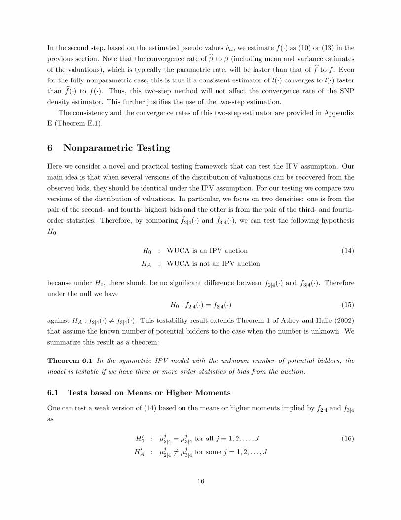
6 Nonparametric Testing

Here we consider a novel and practical testing framework that can test the IPV assumption. Our

main idea is that when several versions of the distribution of valuations can be recovered from the

observed bids, they should be identical under the IPV assumption. For our testing we compare two

versions of the distribution of valuations. In particular, we focus on two densities: one is from the

pair of the second- and fourth- highest bids and the other is from the pair of the third- and fourth-

order statistics. Therefore, by comparing f2j4(�) and f3j4(�), we can test the following hypothesisH0

H0 : WUCA is an IPV auction (14)

HA : WUCA is not an IPV auction

because under H0, there should be no signi�cant di¤erence between f2j4(�) and f3j4(�). Thereforeunder the null we have

H0 : f2j4(�) = f3j4(�) (15)

against HA : f2j4(�) 6= f3j4(�). This testability result extends Theorem 1 of Athey and Haile (2002)

that assume the known number of potential bidders to the case when the number is unknown. We

summarize this result as a theorem:

Theorem 6.1 In the symmetric IPV model with the unknown number of potential bidders, the

model is testable if we have three or more order statistics of bids from the auction.

6.1 Tests based on Means or Higher Moments

One can test a weak version of (14) based on the means or higher moments implied by f2j4 and f3j4as

H 00 : �j2j4 = �

j3j4 for all j = 1; 2; : : : ; J (16)

H 0A : �j2j4 6= �

j3j4 for some j = 1; 2; : : : ; J

16

where �j2j4 =R vv v

jf2j4(v)dv and �j3j4 =

R vv v

jf3j4(v)dv, since (14) implies (16). One can compare

estimates of several moments implied by f2j4 and f3j4 and test for the signi�cance of di¤erence in

each pair of moments by constructing standardized test statistics. A di¢ culty of implementing

this approach will be to re�ect into the test statistics the fact that one uses pre-estimated density

functions f2j4 and f3j4 to estimate the moments.

6.2 Comparison of Densities Using the Pseudo Kullback-Leibler DivergenceMeasure

We are interested in testing the equivalence of two densities f2j4 and f3j4 where these densities

are estimated from (11) and (13), respectively using the SNP density estimation. One measure to

compare f2j4 and f3j4 will be the integrated squared error given by Is(f2j4(z),f3j4(z)) =RV(f2j4(z)�

f3j4(z))2dz. Under the null we have Is(f2j4(z),f3j4(z)) = 0. Li (1996) develops a test statistic

of this sort when both densities are estimated using a kernel method. Other useful measures for

the distance of two density functions are the Kullback-Leibler (KL) information distance and the

Hellinger metric. For testing of (e.g.) serial independence using densities, it is well known that test

statistics based on these two measures have better small sample properties than those based on a

squared distance in terms of a second order asymptotic theory. The KL measure is entertained in

Ullah and Singh (1989), Robinson (1991), and Hong and White (2005) when they test the a¢ nity

of two densities. The KL measure is de�ned by

IKL =

ZV

�ln f2j4(z)� ln f3j4(z)

�f2j4(z)dz (17)

or IKL =RV�ln f3j4(z)� ln f2j4(z)

�f3j4(z)dz, which is equally zero under the null and has positive

values under the alternative (see Kullback and Leibler 1951). One could construct a test statistic

using a sample analogue of (17):

IKL( bf2j4; bf3j4) = ZV(ln bf2j4(z)� ln bf3j4(z))d bF2j4(z).

Now suppose fevtgTt=1 in the data are the second-highest order statistics. Then, one may expectRV(ln

bf2j4(z)� ln bf3j4(z))d bF2j4(z) � 1T

PTt=1

�ln bf2j4(evt)� ln bf3j4(evt)� but this is not true because evt

follows the distribution of the second-highest order statistic, not that of valuations F2j4. We can,

however, argue that1

T

PTt=1

�ln bf2j4(evt)� ln bf3j4(evt)�

is still useful in terms of comparing two densities because under the null the following object equals

to zero ZV

�ln f2j4(z)� ln f3j4(z)

�g(n�1:n)(z)dz (18)

17

where g(n�1:n)(z) is the density of the second-highest order statistic of the n sample.14 Note that

(18) is not a distance measure since it can take negative values but still can serve as a divergence

measure.

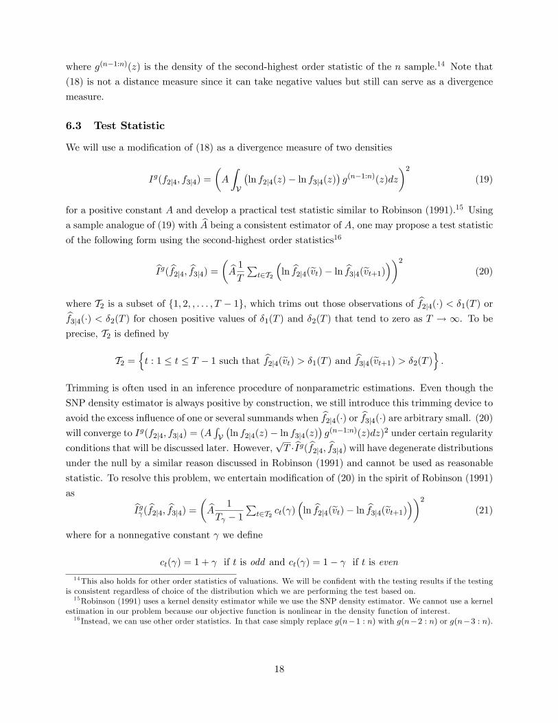
6.3 Test Statistic

We will use a modi�cation of (18) as a divergence measure of two densities

Ig(f2j4; f3j4) =

�A

ZV

�ln f2j4(z)� ln f3j4(z)

�g(n�1:n)(z)dz

�2(19)

for a positive constant A and develop a practical test statistic similar to Robinson (1991).15 Using

a sample analogue of (19) with bA being a consistent estimator of A, one may propose a test statisticof the following form using the second-highest order statistics16

bIg( bf2j4; bf3j4) = � bA 1T Pt2T2

�ln bf2j4(evt)� ln bf3j4(evt+1)��2 (20)

where T2 is a subset of f1; 2; ; : : : ; T � 1g, which trims out those observations of bf2j4(�) < �1(T ) orbf3j4(�) < �2(T ) for chosen positive values of �1(T ) and �2(T ) that tend to zero as T ! 1. To beprecise, T2 is de�ned by

T2 =nt : 1 � t � T � 1 such that bf2j4(evt) > �1(T ) and bf3j4(evt+1) > �2(T )o .

Trimming is often used in an inference procedure of nonparametric estimations. Even though the

SNP density estimator is always positive by construction, we still introduce this trimming device to

avoid the excess in�uence of one or several summands when bf2j4(�) or bf3j4(�) are arbitrary small. (20)will converge to Ig(f2j4; f3j4) = (A

RV�ln f2j4(z)� ln f3j4(z)

�g(n�1:n)(z)dz)2 under certain regularity

conditions that will be discussed later. However,pT �bIg( bf2j4; bf3j4) will have degenerate distributions

under the null by a similar reason discussed in Robinson (1991) and cannot be used as reasonable

statistic. To resolve this problem, we entertain modi�cation of (20) in the spirit of Robinson (1991)

as bIg ( bf2j4; bf3j4) = � bA 1

T � 1Pt2T2 ct( )

�ln bf2j4(evt)� ln bf3j4(evt+1)��2 (21)

where for a nonnegative constant we de�ne

ct( ) = 1 + if t is odd and ct( ) = 1� if t is even

14This also holds for other order statistics of valuations. We will be con�dent with the testing results if the testingis consistent regardless of choice of the distribution which we are performing the test based on.15Robinson (1991) uses a kernel density estimator while we use the SNP density estimator. We cannot use a kernel

estimation in our problem because our objective function is nonlinear in the density function of interest.16 Instead, we can use other order statistics. In that case simply replace g(n�1 : n) with g(n�2 : n) or g(n�3 : n).

18

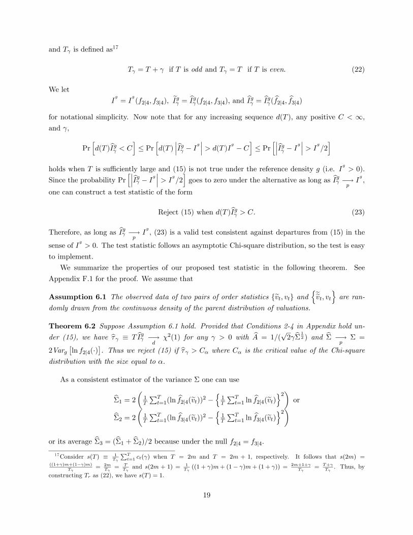
and T is de�ned as17

T = T + if T is odd and T = T if T is even. (22)

We let

Ig= I

g(f2j4; f3j4); eIg = bIg (f2j4; f3j4), and bIg = bIg ( bf2j4; bf3j4)

for notational simplicity. Now note that for any increasing sequence d(T ), any positive C < 1,and ,

Prhd(T )bIg < Ci � Pr hd(T ) ���bIg � Ig ��� > d(T )Ig � Ci � Pr h���bIg � Ig ��� > Ig=2i

holds when T is su¢ ciently large and (15) is not true under the reference density g (i.e. Ig> 0).

Since the probability Prh���bIg � Ig ��� > Ig=2i goes to zero under the alternative as long as bIg �!

pIg,

one can construct a test statistic of the form

Reject (15) when d(T )bIg > C. (23)

Therefore, as long as bIg �!pIg, (23) is a valid test consistent against departures from (15) in the

sense of Ig> 0. The test statistic follows an asymptotic Chi-square distribution, so the test is easy

to implement.

We summarize the properties of our proposed test statistic in the following theorem. See

Appendix F.1 for the proof. We assume that

Assumption 6.1 The observed data of two pairs of order statistics fevt; vtg and neevt; vto are ran-domly drawn from the continuous density of the parent distribution of valuations.

Theorem 6.2 Suppose Assumption 6.1 hold. Provided that Conditions 2-4 in Appendix hold un-der (15), we have b� � T bIg �!

d�2(1) for any > 0 with bA = 1=(

p2 b� 1

2 ) and b� �!p� =

2Varg�ln f2j4(�)

�. Thus we reject (15) if b� > C� where C� is the critical value of the Chi-square

distribution with the size equal to �.

As a consistent estimator of the variance � one can use

b�1 = 2� 1T

PTt=1(ln

bf2j4(evt))2 � n 1T PTt=1 ln

bf2j4(evt)o2� or

b�2 = 2� 1T

PTt=1(ln

bf3j4(evt))2 � n 1T PTt=1 ln

bf3j4(evt)o2�or its average b�3 = (b�1 + b�2)=2 because under the null f2j4 = f3j4.17Consider s(T ) � 1

T

PTt=1 ct( ) when T = 2m and T = 2m + 1, respectively. It follows that s(2m) =

((1+ )m+(1� )m)T

= 2mT

= TT

and s(2m + 1) = 1T ((1 + )m+ (1� )m+ (1 + )) = 2m+1+

T = T+

T . Thus, by

constructing Tr as (22), we have s(T ) = 1.

19

To implement the proposed test we need to pick a value for . Even though the test is valid

for any choice of > 0 asymptotically, it is not necessarily true for �nite samples (see Robinson

1991). The testing result could be sensitive to the choice of . Robinson (1991) suggests taking

between 0 and 1. He argues that the power of the test is inversely related with the value of but

one should not take too small for which the asymptotic normal approximation breaks down (i.e.

the statistic does not have a standard asymptotic distribution).

7 Empirical Results

7.1 Monte Carlo Experiments

In this section, we perform several Monte Carlo experiments to illustrate the validity of our esti-

mation strategy. We generate arti�cial data of T = 1000 auctions using the following design. The

number of potential bidders, fNig, are drawn from a Binomial distribution with (n; p) = (50; 0:1)

for each auction (t = 1; : : : ; T ). Nt potential bidders are assumed to value the object according to:

lnVti = �1X1t + �2X2t + �3X3t + Vti; (24)

where �1 = 1, �2 = �1, �3 = 0:5, X1t � N(0; 1), X2t � Exp(1), X3t = X1t � X2t + 1, andVti � Gamma(9; 3).18 X�t�s represent the observed auction heterogeneity and Vti is bidder i�s

private information in auction t, whose distribution is of our primary interest. To consider the case

of binding reserve prices, we also generate the reserve prices as

lnRt = �1X1t + �2X2t + �3X3t + �t;

where �t � Gamma(9; 3) � 2. Note that by construction Vti and Rt are independent conditionalon X�t�s. An arti�cial bidder bids only when Vti is greater than Rt. Here we assume our imaginaryresearcher does not know the presence of potential bidders with valuations below Rt. Thus, in

each experiment, she has a data set of X�t�s, and the second-, the third-, and the fourth-highest

bids among observed bids. Auctions with fewer than four actual bidders are dropped. Hence, our

researcher has the sample size less than T = 1000 (on average T = 680 with 50 repetitions). Our

researcher estimates �1, �2, �3 and f(�) (pdf of Vti) by varying the approximation order (K) of theSNP estimator, from 0 to 7 without knowing the speci�cation of the distribution of Vti in (24). Weused the two-step estimation approach to reduce the computational burden. Among K between

0 to 7, we report estimation results with K = 6 because it performs best in this Monte Carlo

experiments.

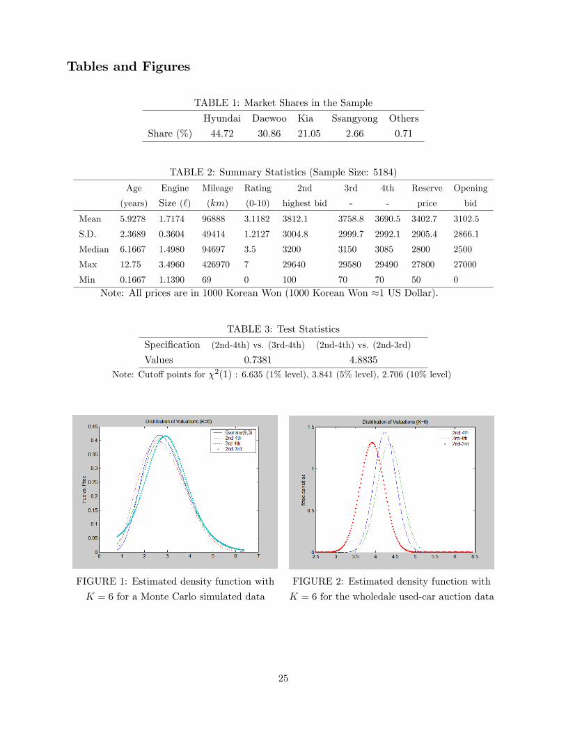
Figure 1 illustrates a performance of the estimator. By construction of our MC design, the

three versions of density function estimates for valuations should not be statistically di¤erent from

each other (one is based on the pair of (2nd; 4th) order statistics and others are based on the pair

18Note that for V � Gamma(9; 3), E(V ) = 3 and V ar(V ) = 1.

20

of (3rd; 4th) and (2nd; 3rd).)

7.2 Estimation Results

We discuss estimation and testing results using the real auction data. In the �rst stage regression

obtaining the function of the observed heterogeneity l(x), we used a linear speci�cation to minimize

the computational burden of the SNP density estimation. We use the following covariates: X1 is

the vector of dummy variables indicating the car make such as Hyundai, Daewoo, Kia or Others;

X2 is the age; X3 is the engine size; X4 is the mileage; X5 is the rating by the auction house; X6 is

the dummy for the transmission type; X7 is the dummy for the fuel type; X8 is the dummy for the

popular colors; X9 and X10 are the dummy variables for the options. Table 2 presents summary

statistics for some of these covariates and several order statistics over the reserve price.

We estimate l(x) separately for each car make such that l(x) = lm(x) = x0�(m) where m denotes

the car make and obtain the estimate of pseudo valuations as residuals. Table A1 provides the �rst-

stage estimates with the linear speci�cation. The signs for the coe¢ cient of age, transmission, engine

size, and rating variables look reasonable and the coe¢ cients are signi�cant, while the interpretation

of coe¢ cient signs for the fuel type, mileage, colors, options, and title remaining is not so clear.

Based on the estimated pseudo valuations, in the second step, we estimate the distribution of

valuations using three di¤erent pairs of order statistics (2nd; 4th), (3rd; 4th), and (2nd; 3rd). Figure 2

illustrates the estimated density function of valuations using the linear estimation in the �rst stage.

With these three nonparametric estimates of the distribution, we conduct our nonparametric test of

the IPV. Testing results using our test statistics de�ned in (21) are rather mixed depending on which

distributions we compare but overall it does support the IPV. When we compare the estimated

distribution of valuations using (2nd; 4th) vs. (3rd; 4th) order statistics, clearly we do not reject

the IPV even under the 10% signi�cance level. However, when the estimated distributions using

(2nd; 4th) vs. (2nd; 3rd) order statistics are compared, we reject the IPV under the 5% signi�cance

while do not reject under the 1% level. Values for the test statistic are provided in Table 3.

As we note in Figure 2 and Table 3, the estimated distribution using the pair of the 2nd- and the

3rd-highest order statistics is quite di¤erent from the others. Moreover, we note that the estimation

results using the pair of (2nd; 3rd) order statistics are substantially varying over di¤erent settings

(e.g. using di¤erent approximation order K and di¤erent initial values for estimation). Examining

the bidding data, we �nd that the number of observations for which di¤erences between the 2nd-

and the 3rd-highest order statistics are small is much larger, compared to other pairs of order

statistics, which may have contributed to the numerical instability in �nite samples.19 Note that

by construction of the conditional density pk1jk2(evjv) in (2), identi�cation of the distribution ofvaluations becomes stronger when the di¤erences between order statistics are larger. We therefore

conclude that the testing results based on the estimated distributions using (2nd; 4th) vs. (3rd; 4th)

19The di¤erence between the 2nd- and the 3rd-highest order statistics was not larger than 30 US dollars in 3,045observations out of the total 5,184 observations while such observation counts were 1,688 for the 3nd- and the 4rd-highest order statistics and were 441 for the 2nd- and the 4rd-highest order statistics.

21

order statistics are more reliable, which clearly support the IPV. Note, however, that a high value of

the test statistic comparing the estimated distributions from (2nd; 4th) vs. (2nd; 3rd) order statistics

illustrates the power of our proposed test. Table 4 reports additional testing results by varying the

approximation order K in the SNP density and also the testing parameter .20

8 Discussions and Implications

8.1 Discussion of the Testing Result

In this section, we discuss the result of our IPV test. With our estimates, we do not reject the null

hypothesis of IPV in our auction. We can interpret this result as an evidence of no informational

dependency among bidders about the valuations of observed characteristics of a used-car and no

e¤ect of any unobserved (to an econometrician) characteristics on valuations. Our conjecture is

that this situation may arise because each dealer operates in her own local market and there is no

interdependency among those markets, or when a dealer has a speci�c demand (order) from a �nal

buyer on hand. This can happen when a dealer gets an order for a speci�c used-car but does not

have one in stock or when a consumer looks up the item list of an auction and asks a dealer to buy

a speci�c car for her.

If the assumption of IPV were rejected, it could have been due to a violation of the independence

assumption or a violation of the private value assumption. This could happen when a dealer does

not have a speci�c demand on hand, but she anticipates some demand in near future from the

analysis of the overall performance of the national market since every used-car won in the auction

is to be resold to a �nal consumer. In this case, a dealer may have some incentives to �nd out other

dealers�opinions about the prospect of the national market. With our data, we �nd no evidence

to support this hypothesis.

8.2 Bounds Estimation

We have disregarded the minimum increment of around 30 dollars in WUCA. In this section, we

discuss how to obtain the bounds of the distribution of valuations incorporating the minimum

increment. The bounds considered here is much simpler than those considered in Haile and Tamer

(2003), since in WUCA any order statistic of valuations other than the �rst highest one is bounded

as

b(i:n) � v(i:n) � b(i:n) +�; for all i = 1; : : : ; n� 1; (25)

where (i : n) denotes the ith order statistic out of the n sample and � depicts the minimum

increment. By the �rst-order stochastic dominance, noting Gb(i:n)+�(v) = Gb(i:n)(v � �), (25)implies

Gb(i:n)(v) � Gv(i:n)(v) � Gb(i:n)(v ��);20Table 3 is the case with = 1=2. We found similar results with di¤erent values of unless it is too small (see

Table 4).

22

where G�(�) denotes the distribution of the order statistics. Then, using the identi�cation methoddiscussed in Section 4, we have

Fb(v) � Fv(v) � Fb(v ��) �= Fb(v)� fb(v)�;

where Fb(�) and fb(�) are the CDF and PDF, respectively, of valuations based on observed bids. Thelast weak equality comes from the �rst-order Taylor series expansion. Therefore, we can estimate

the bounds of Fv(v) as

Fb(v) � Fv(v) � Fb(v)� fb(v)�;

where fb(�) the SNP estimator based on the certain observed order statistics of bids, Fb(x) =R xmin(b) fb(v)dv and min(b) is the minimum among the observed bids considered.

8.3 Combining Several Order Statistics

Once we show the several versions of estimates for the distribution of valuations are statistically

not di¤erent each other, we may obtain a more e¢ cient estimate by combining them. One way

to do this is to consider the joint density function of two or more order statistics conditional on a

certain order statistic. Suppose we have the kth1 , kth2 , and k

th3 -highest order statistics, which are the

(n � k1 � 1)th, (n � k2 � 1)th, (n � k3 � 1)th order statistics respectively (1 � k1 < k2 < k3 � n).Denote the joint density of these three order statistics as ~g(k1;k2;k3:n)(�) - we use this notation ~g(�)

to distinguish it from g(�) so that ki denotes the kthi highest order statistics:

~g(k1;k2;k3:n)(ev;eev; v) = n!

(n� k3)!(k3 � k2 � 1)!(k2 � k1 � 1)!(k1 � 1)!�F (v)n�k3f(v)[F (eev)� F (v)]k3�k2�1f(eev)[F (ev)� F (eev)]k2�k1�1f(ev)[1� F (ev)]k1�1;

where eV denotes the kth1 -, eeV denotes the kth2 -, and V denotes the kth3 -highest order statistics. Usingthis joint density function together with the marginal density (1), we obtain the conditional joint

density of the kth1 and the kth2 -highest order statistics conditional on the kth3 -highest statistics as

p(k1;k2)jk3(ev;eevjv)= (k3�1)!

(k3�k2�1)!(k2�k1�1)!(k1�1)![F (eev)�F (v)]k3�k2�1f(eev)[F (ev)�F (eev)]k2�k1�1f(ev)[1�F (ev)]k1�1

[1�F (v)]k3�1

= (k3�1)!(k3�k2�1)!(k2�k1�1)!(k1�1)! [(1� F (v))F (

eevjv)]k3�k2�1� f(eevjv)(1� F (v))[(F (evjv)� F (eevjv))(1� F (v))]k2�k1�1 � f(evjv)(1�F (v))[(1�F (evjv))(1�F (v))]k1�1

[1�F (v)]k3�1

= (k3�1)!(k3�k2�1)!(k2�k1�1)!(k1�1)!F (

eevjv)k3�k2�1f(eevjv)� [F (evjv)� F (eevjv)](k3�k1)�(k3�k2)�1f(evjv)[1� F (evjv)](k3�1)�(k3�k1)

= g(k3�k1;k3�k2:k3�1)(ev;eevjv);(26)

23

where F (�jv) and f(�jv)(g(�jv)) are the truncated CDF and PDF�s truncated at v respectively. Thelast equality comes from the joint density of the j-th and i-th order statistics (n � j > i � 1),

g(j;i:n)(a; b) =n![F (b)]i�1[F (a)� F (b)]j�i�1[1� F (a)]n�jf(b)f(a)

(i� 1)!(j � i� 1)!(n� j)! Ifa>bg

where a and b are the j-th and i-th order statistics, respectively by letting j = k3� k1, i = k3� k2,and n = k3 � 1. Therefore we can interpret p(k1;k2)jk3(�) as the joint density of (k3 � k1)th and(k3 � k2)th order statistics from a sample of size equal to (k3 � 1). When (k1; k2; k3) = (2; 3; 4),

(26) becomes

p(2;3)j4(ev;eevjv) = 6f(eev)f(ev)[1� F (ev)][1� F (v)]�3: (27)

Based on (27), one can estimate the distribution of valuations f(�) similarly with the methodproposed in Section 5.1. The resulting estimator will be more e¢ cient than bf2j4(�) or f3j4(�) in thesense that it uses more information.

9 Conclusions

In this paper we developed a practical nonparametric test of symmetric IPV in ascending auctions

when the number of potential bidders is unknown. Our key idea for testing is that because any

pair of order statistics can identify the value distribution, three or more order statistics can identify

two or more value distributions and under the symmetric IPV, those value distributions should

be identical. Therefore, testing the symmetric IPV is equivalent to testing the similarity of value

distributions obtained from di¤erent pairs of order statistics. This extends the testability of the

symmetric IPV of Athey and Haile (2002) that assume the known number of potential bidders to

the case when the number is unknown.

Using the proposed methods we conducted a structural analysis of ascending-price auctions

using a new data set on a wholesale used-car auction, in which there is no jump bidding. Exploiting

the data, we estimated the distribution of bidders�valuations nonparametrically within the IPV

paradigm. We can implement our test because the data enables us to exploit information from

observed losing bids. We �nd that the null hypothesis of symmetric IPV is arguably supported

with our data after controlling for observed auction heterogeneity. The richness of our data has

allowed us to conduct a structural analysis that bridges the gap between theoretical models based

on Milgrom and Weber (1982) and real-world ascending-price auctions.

In this paper, we have considered the auction as a collection of isolated single-object auctions. In

future work, we will look at the data more closely in the alternative environments. For example, we

will examine intra-day dynamics of auctions with daily budget constraints for bidders, or possible

complementarity and substitutability in a multi-object auction environment. Another possibility

is to consider an asymmetric IPV paradigm noting that information of winning bidders�identities

is available in the data.

24

Tables and Figures

TABLE 1: Market Shares in the Sample

Hyundai Daewoo Kia Ssangyong Others

Share (%) 44:72 30:86 21:05 2:66 0:71

TABLE 2: Summary Statistics (Sample Size: 5184)

Age Engine Mileage Rating 2nd 3rd 4th Reserve Opening

(years) Size (`) (km) (0-10) highest bid - - price bid

Mean 5.9278 1.7174 96888 3.1182 3812.1 3758.8 3690.5 3402.7 3102.5

S.D. 2.3689 0.3604 49414 1.2127 3004.8 2999.7 2992.1 2905.4 2866.1

Median 6.1667 1.4980 94697 3.5 3200 3150 3085 2800 2500

Max 12.75 3.4960 426970 7 29640 29580 29490 27800 27000

Min 0.1667 1.1390 69 0 100 70 70 50 0

Note: All prices are in 1000 Korean Won (1000 Korean Won �1 US Dollar).

TABLE 3: Test Statistics

Speci�cation (2nd-4th) vs. (3rd-4th) (2nd-4th) vs. (2nd-3rd)

Values 0:7381 4:8835

Note: Cuto¤ points for �2(1) : 6.635 (1% level), 3.841 (5% level), 2.706 (10% level)

FIGURE 1: Estimated density function with

K = 6 for a Monte Carlo simulated data

FIGURE 2: Estimated density function with

K = 6 for the wholedale used-car auction data

25

TABLE 4: Test Statistics Comparing Distributions of Valuations from (2nd-4th) vs. (3rd-4th)

Speci�cation of the SNP K=0 K=2 K=4 K=6

Testing para ( )

= 0:2 1.5971 1.7245 1.6610 1.3494

= 0:4 0.9703 1.0098 0.9845 0.8273

= 0:5 0.8635 0.8897 0.8703 0.7381

= 0:6 0.7958 0.8138 0.7981 0.6814

= 0:8 0.7151 0.7237 0.7122 0.6138Note: Cuto¤ points for �2(1) : 6.635 (1% level), 3.841 (5% level), 2.706 (10% level)

References

[1] Ai, C. and X. Chen (2003), �E¢ cient Estimation of Models With Conditional Moment Re-strictions Containing Unknown Functions,�Econometrica, v71, No.6, 1795-1843.

[2] Arnold, B., Balakrishnan, N., and Nagaraja, H. (1992), A First Course in Order Statistics.(New York: John Wiley & Sons.)

[3] Athey, S. and Haile, P. (2002), �Identi�cation of Standard Auction Models,�Econometrica,70(6), 2107-2140.

[4] Athey, S. and Haile, P. (2005), �Nonparametric Approaches to Auctions,� forthcoming in J.Heckman and E. Leamer, eds., Handbook of Econometrics, Vol. 6, Elsevier.

[5] Athey, S. and Levin, J. (2001), �Information and Competition in U.S. Forest Service TimberAuctions,�Journal of Political Economy, 109, 375-417.

[6] Bikhchandani, S., Haile, P. and Riley, J. (2002), �Symmetric Separating Equilibria in EnglishAuctions,�Games and Economic Behavior, 38, 19-27.

[7] Bikhchandani, S. and Riley, J. (1991), �Equilibria in Open Common Value Auctions,�Journalof Economic Theory, 53, 101-130.

[8] Bikhchandani, S. and Riley, J. (1993), �Equilibria in Open Auctions,�mimeo, UCLA.

[9] Campo, S., Perrigne, I., and Vuong, Q. (2003) �Asymmetry in First-Price Auctions WithA¢ liated Private Values,�Journal of Applied Econometrics, 18, 179-207.

[10] Chen, X. (2007), �Large Sample Sieve Estimation of Semi-Nonparametric Models,�Handbookof Econometrics, V.6.

[11] Coppejans, M. and Gallant, A. R. (2002), �Cross-validated SNP density estimates,�Journalof Econometrics, 110, 27-65.

[12] David, H. A. (1981), Order Statistics. Second Edition. (New York: John Wiley & Sons.)

26

[13] Fenton V. M. and Gallant, A. R. (1996), �Convergence Rates of SNP Density Estimators,�Econometrica, 64, 719-727.

[14] Gallant, A. R. and Nychka, D. (1987), �Semi-nonparametric Maximum Likelihood Estima-tion,�Econometrica, 55, 363-390.

[15] Gallant, A. R. and G. Souza (1991), �On the Asymptotic Normality of Fourier Flexible FormEstimates,�Journal of Econometrics, 50, 329-353.

[16] Guerre, E., Perrigne, I., and Vuong, Q. (2000), �Optimal Nonparametric Estimation of First-Price Auctions,�Econometrica, 68, 525-574.

[17] Guerre, E., Perrigne, I., and Vuong, Q. (2009), �Nonparametric Identi�cation of Risk Aversionin First-Price Auctions Under Exclusion Restrictions,�Econometrica, 77(4), 1193-1228.

[18] Haile, P., Hong, H., and Shum, M. (2003), �Nonparametric Tests for Common Values in First-Price Sealed-Bid Auctions,�NBER Working Paper No. 10105.

[19] Haile, P. and Tamer, E. (2003), �Inference with an Incomplete Model of English Auctions,�Journal of Political Economy, 111(1), 1-51.

[20] Hansen, B. (2004), �Nonparametric Conditional Density Estimation,�Working paper, Univer-sity of Wisconsin-Madison.

[21] Harstad, R. and Rothkopf, M. (2000), �An �Alternating Recognition�Model of English Auc-tions,�Management Science, 46, 1-12.

[22] Hendricks, K. and Paarsch, H. (1995), �A Survey of Recent Empirical Work concerning Auc-tions,�Canadian Journal of Economics, 28, 403-426.

[23] Hendricks, K., Pinkse, J., and Porter, R. (2003), �Empirical Implications of Equilibrium Bid-ding in First-Price, Symmetric, Common Value Auctions,�Review of Economic Studies, 70(1),115-146.

[24] Hoe¤ding, W. (1963), �Probability Inequalities for Sums of Bounded Random Variables,�Journal of the American Statistical Association, 58, 13-30.

[25] Hong, H., and Shum, M. (2003), �Econometric Models of Asymmetric Ascending Auctions,�Journal of Econometrics, 112, 327-358.

[26] Hong, Y.-M. and White, H. (2005), �Asymptotic Distribution Theory for an Entropy-BasedMeasure of Serial Dependence,�Econometrica, 73, 837-902.

[27] Hu, Y., D. McAdams, and M. Shum (2013), �Identi�cation of First-Price Auction Models withNon-Separable Unobserved Heterogeneity,�Journal of Econometrics, 174(2), 186-193.

[28] Izmalkov, S. (2003), �English Auctions with Reentry,�mimeo, MIT.

[29] Krasnokutskaya, E. (2011), �Identi�cation and Estimation of Auction Models with UnobservedHeterogeneity,�Review of Economic Studies, 78(1), 293-327.

[30] Kim, K. (2007), �Uniform Convergence Rate of the SNP Density Estimator and Testing forSimilarity of Two Unknown Densities,�Econometrics Journal, 10(1), 1-34.

27

[31] Kullback, S. and Leibler, R.A. (1951), �On Information and Su¢ ciency,�Ann. Math. Stat.,22, 79-86.

[32] La¤ont and Vuong (1996)

[33] La¤ont, J.-J. (1997), �Game Theory and Empirical Economics: The Case of Auction Data,�European Economic Review, 41, 1-35.

[34] Larsen, B. (2012), �The E¢ ciency of Dynamic, Post-Auction Bargaining: Evidence fromWholesale Used-Auto Auctions,�MIT job market paper.

[35] Li, Q. (1996), �Nonparametric Testing of Closeness between Two Unknown Distribution Func-tions,�Econometric Reviews, 15, 261-274.

[36] Li, T., Perrigne, I., and Vuong, Q. (2000), �Conditionally Independent Private Information inOCS Wildcat Auctions,�Journal of Econometrics, 98, 129-161.

[37] Li, T., Perrigne, I., and Vuong, Q. (2002), �Structural Estimation of the A¢ liated PrivateValue Auction Model,�RAND Journal of Economics, 33, 171-193.

[38] Lorentz, G. (1986), Approximation of Functions, New York: Chelsea Publishing Company.

[39] Matzkin, R. (2003), �Nonparametric Estimation of Nonadditive Random Functions,�Econo-metrica, 71(5), 1339-1375.

[40] Milgrom, P. and Weber, R. (1982), �A Theory of Auctions and Competitive Bidding,�Econo-metrica, 50, 1089-1122.

[41] Myerson, R. (1981), �Optimal Auction Design,�Math. Operations Res., 6, 58-73.

[42] Newey, W. (1997), �Convergence Rates and Asymptotic Normality for Series Estimators,�Journal of Econometrics, 79, 147-168.

[43] Newey, W., J. Powell and F. Vella (1999), �Nonparametric Estimation of Triangular Simulta-neous Equations Models,�Econometrica, 67, 565-603.

[44] Paarsch, H. (1992), �Deciding Between the Common and Private Value Paradigms in EmpiricalModels of Auctions,�Journal of Econometrics, 51, 191-215.

[45] Riley, J. (1988), �Ex Post Information in Auctions,�Review of Economic Studies, 55, 409-429.

[46] Roberts, J (2013), �Unobserved Heterogeneity and Reserve Prices in Auctions,� forthcomingin RAND Journal of Economics.

[47] Robinson, P. M. (1991), �Consistent Nonparametric Entropy-Based Testing,�Review of Eco-nomic Studies, 58, 437-453.

[48] Song, U. (2005), �Nonparametric Estimation of an eBay Auction Model with an UnknownNumber of Bidders,� Economics Department Discussion Paper 05-14, University of BritishColumbia.

[49] Ullah, A. and Singh, R.S. (1989), �Estimation of a Probability Density Function with Applica-tions to Nonparametric Inference in Econometrics,�in B. Raj (ed.) Advances in Econometricsand Modelling, Kluwer Academic Press, Holland.

28

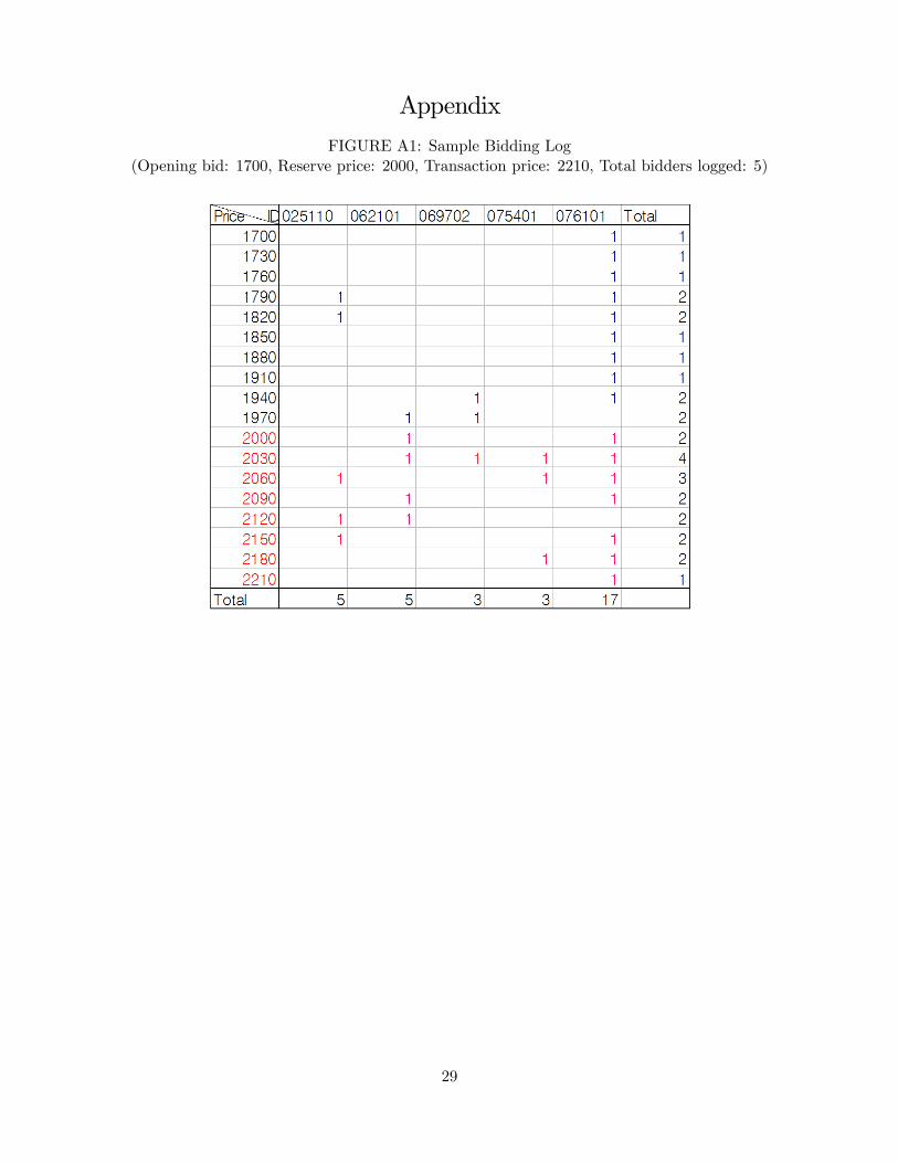
Appendix

FIGURE A1: Sample Bidding Log(Opening bid: 1700, Reserve price: 2000, Transaction price: 2210, Total bidders logged: 5)

29

TABLE A1: First-Stage Estimation Results (Linear model)

Maker Covariate Estimate Standard ErrorHyundai Intercept 5.2247 0.0945(T=1676) Age -0.2439 0.0058

Engine Size (l) 0.7760 0.0367Mileage (104km) 0.0004 0.0022Rating 0.1241 0.0082Automatic 0.2874 0.0192Gasoline 0.0155 0.0381Popular Colors 0.0567 0.0184Best Options 0.2441 0.0316Better Options 0.1178 0.0210

Daewoo Intercept 5.2821 0.0991(T=1186) Age -0.3369 0.0062

Engine Size (l) 0.9470 0.0479Mileage (104km) -0.0108 0.0027Rating 0.0508 0.0101Automatic 0.2430 0.0215Gasoline 0.3306 0.0374Popular Colors -0.0551 0.0191Best Options 0.1344 0.0299Better Options 0.0244 0.0218

Kia & etc. Intercept 5.2698 0.1082(T=964) Age -0.2234 0.0070

Engine Size (l) 0.5731 0.0390Mileage (104km) 0.0054 0.0026Rating 0.1004 0.0111Automatic 0.3347 0.0247Gasoline -0.1943 0.0414Popular Colors 0.0278 0.0225Best Options 0.3947 0.0424Better Options 0.2062 0.0273

A Normalized Hermite Polynomials

Here are examples of the normalized Hermite polynomials that we use to approximate the densityof valuations. These are generated by the recursive system in (8). Note that

R1�1H

2j dz = 1 andR1

�1HjHkdz = 0; j 6= k by construction.

H1 =14p2�e

� 14z2 , H2 = z

4p2�e� 14z2

H3 =1

2 4p2�

�z2p2�

p2�e�

14z2 , H4 = 1

6 4p2�

�z3p6� 3z

p6�e�

14z2

H5 =1

12 4p2�

�3p6� 6z2

p6 + z4

p6�e�

14z2

H6 =1

60 4p2�

�15z

p30� 10z3

p30 + z5

p30�e�

14z2

H7 =1

60 4p2�

�45z2

p5� 15

p5� 15z4

p5 + z6

p5�e�

14z2 :

30

B Nonparametric Extension: the Observed Heterogeneity

In the main text we have assumed that l(�) belongs to a parametric family. Here we consider anonparametric speci�cation of l(�). We can approximate the unknown function l(Xt) in (3) usinga sieve such as power series or splines (see e.g. Chen 2007). We approximate the function space Lcontaining the true l(�) with the following power series sieve space LT

LT = fl(X)jl(X) = Rk1(T )(X)0� for all � satisfying klk� 1 � c1g;

where Rk1(X) is a triangular array of some basis polynomials with the length of k1. Here k � k� denotes the Hölder norm:

jjgjj� = supxjg(x)j+ max

a1+a2+:::adx= supx 6=x0

jrag(x)�rag(x0)j(jjx� x0jjE) �

<1;

where rag(x) � @a1+a2+:::adx

@xa11 :::@x

adxdx

g(x) with the largest integer smaller than . The Hölder ball (with

radius c) � c (X ) is de�ned accordingly as

� c (X ) � fg 2 � (X ) : jjgjj� � c <1g

and we take the function space L �� 1c1 (X ). Functions in � c (X ) can be approximated well by

various sieves such as power series, Fourier series, splines, and wavelets.The functions in LT is getting dense as T !1 but not that fast, i.e. k1 !1 as T !1 but

k1=T ! 0. Then, according to Theorem 8, p.90 in Lorentz (1986), there exists a �k1 such that forRk1(x) on the compact set X (the support of X) and a constant c121

supx2X

jl(x)�Rk1(x)0�k1 j < c1k1� [ 1]

dx ; (28)

where [s] is the largest integer less than s and dx is the dimension of X. Thus, we approximate thepseudo-value Vti in (3) as

Vti = lnVti � lk1(Xt); (29)

where lk1(x) = Rk1(x)0�k1 .

Speci�cally, we consider the following polynomial basis considered by Newey, Powell, and Vella(1999). First let � = (�1; : : : ; �dx)

0 denote a vector of nonnegative integers with the norm j�j =Pdxj=1 �j , and let x

� �Qdxj=1(xj)

�j . For a sequence f�(k)g1k=1 of distinct vectors, we construct atensor-product power series sieve as Rk1(x) = (x�(1); : : : ; x�(k1))0. Then, replacing each power x� bythe product of orthonormal univariate polynomials of the same order, we may reduce collinearity.Note that the approximation precision depends on the choice of smoothing parameter k1. Wediscuss how to pick the optimal length of series k�1 in Appendix C.

C Choosing the optimal approximation parameters

Instead of using the Leave-one-out method for cross-validation, we will partition the data into Pgroups, making the size of each group as equal as possible and use the Leave-one partition-outmethod. We do this because it will be computationally too expensive to use the Leave-one-out

21We often suppress the argument T in k1(T ), unless otherwise noted.

31

method, when the sample size is large. We let Tp denote the set of the data indices that belongsto the pth group such that Tp \ Tp0 = � for p 6= p0 and [Pp=1Tp = f1; 2; : : : ; Tg.

C.1 Choosing K�

Coppejans and Gallant (2002) employ a cross-validation method based on the ISE (IntegratedSquared Error) criteria. Let h(x) be a density and h(x) be its estimator. Then the ISE is de�nedby

ISE(h) =Zh2(x)dx� 2

Zh(x)h(x)dx+

Zh(x)2dx =M(1) � 2M(2) +M(3):

We present our approach in terms of �tting p2j4(evjv). We �nd the optimal K� by minimizing anapproximation of the ISE. To approximate the ISE in terms of p2j4(evjv), we use the cross-validationstrategy with the data partitioned into P groups. We �rst approximate M(1) with

cM(1)(K) =

Z(pK2j4(evjv))2d(ev; v) � Z

6(F(K)(ev)� F(K)(v))(F(K)(v)� F(K)(ev))f(K)(ev)

(F(K)(v)� F(K)(v))3

!2d(ev; v);

where f(K)(�) denotes the SNP estimate with the length of the series equal to K and F(K)(z) =R z�1 f(K)(t)dt. For M(2), we consider

cM(2)(K) =1T

PPp=1

Pt2Tp p

p;K2j4 (evtjvt)

� 1T

PPp=1

Pt2Tp

6(Fp;(K)(evt)�Fp;(K)(vt))(Fp;(K)(v)�Fp;(K)(evt))fp;(K)(evt)(Fp;(K)(v)�Fp;(K)(xt))3

;

where fp;(K)(�) denotes the SNP estimate obtained from the sample excluding pth group with the

length of the series K and Fp;(K)(z) =R z�1 fp;(K)(v)dv. Noting M(3) is not a function of K, we

pick K� by minimizing the approximated ISE such that

K� = argminK

cM(1)(K)� 2cM(2)(K).

C.2 Choosing k�1We can use a sample version of the Mean Squared Error criterion for the cross-validation as

SMSE(l) =1

T

PTt=1[l(Xt)� l(Xt)]

2;

where l(�) = Rk1(�)0�. We use the Leave-one partition-out method to reduce the computationalburden. Namely, we estimate the function l(�) from the sample after deleting the pth group withthe length of the series equal to k1 and denote this as lp;k1(�). In the next step, we choose k�1 byminimizing the SMSE such that 22

k�1 = argmink1

1

T

PPp=1

Pt2Tp [lnVt � lp;k1(Xt)]

2 (30)

22Here we can �nd k�1 for particular order statistics or �nd one for over all observed bids. In the latter case, wetake the sum of the minimand in (30) over all observed bids.

32

noting that

SMSE(l) =1

T

PTt=1[l(Xt)� l(Xt)]

2

=1

T

TPt=1[l(Xt)� lnVt]2 + 2

1

T

TPt=1[l(Xt)� lnVt][lnVt � l(Xt)] +

1

T

TPt=1[lnVt � l(Xt)]2 (31)

where the second term of (31) has the mean of zero (assuming E[VtjXt] = 0) and the third term of(31) does not depend on k1.

D Alternative Characterization of the SNP Estimator

We consider an alternative characterization of the SNP density using the speci�cation proposedin Kim (2007) where a truncated version of the SNP density estimator with a compact supportis developed, which turns out to be convenient for deriving the large sample theories. Instead ofde�ning the true density as (5), we follow Kim (2007)�s speci�cation by denoting the true densityas

f(z) = h2f (z)e�z2=2 + �0�(z)=

ZV�(z)dz

where V denotes the support of z. Kim (2007) uses a truncated version of Hermite polynomials toapproximate a density function f with a compact support as

FT =�f : f(z; �) =

�PKj=1 #jwjK(z)

�2+ �0�(z)=

ZV�(z)dz; � 2 �T

�; (32)

where �T =n� = (#1; : : : ; #K(T )) :

PK(T )j=1 #2j + �0 = 1

oand fwjK(z)g are de�ned below following

Kim (2007). First we de�ne wjK(z) = Hj(z)=qR

V H2j (z)dx that is bounded by

supz2V;j�K

jwjK(z)j � supz2V

jHj(z)j =

sminj�K

ZVH2j (v)dv < C

eHfor some constant C < 1, because

RV H

2j (z)dz is bounded away from zero for all j and jHj(z)j <eH uniformly over z and j. Denoting WK(z) = (w1K(z); : : : ; wKK(z))

0, further de�ne QW =RVW

K(z)W

K(z)0dz and its symmetric matrix square root as Q�1=2

W. Now let

WK(z) � (w1K(z); : : : ; wKK(z))0 � Q�1=2WWK(z): (33)

Then by construction, we haveRVW

K(z)WK(z)0 = IK . These truncated and transformed Hermitepolynomials are orthonormalZ

Vw2jK(z)dz = 1;

ZVwjK(z)wkK(z)dz = 0; j 6= k

from which the conditionPK(n)j=1 #

2j + �0 = 1 follows since for any f in FT , we have

RV fdz = 1.

Now de�ne �(K) = supz2V WK(z)

using a matrix norm kAk =ptr(A0A) for a matrix A, which

is the Euclidian norm for a vector. Then, we have �(K) = O(pK) as shown in Lemma G.1. If the

33

range of V are su¢ ciently large, thenRV H

2j (z)dz � 1 and QW � IK and hence wjK � Hj which

implies

supz2V WK(z)

� supz2VqPKj=1H

2j �

pK eH2 = O

�pK�:

The SNP density estimator is now written as (e.g.)

bf2j4 = argmaxf2FT

1

T

PTt=1 lnL(f ; evt; vt) (34)

� argmaxf2FT

1

T

PTt=1 ln

6(F (evt)� F (vt))(1� F (evt))f(evt)(1� F (vt))3

where we de�ne F (z) =R zv f(z)dz. The above maximization problem can be written equivalently

bf2j4 = f(�;b�K) 2 FT ;b�K = argmax�2�T

1

T

TXt=1

lnL(f(�;b�K); evt; vt).E Large Sample Theory of the SNP Density Estimator

First we show the one-to-one mapping between functions in FT and FT de�ned by (7) and (32),respectively. Based on this equivalence, our asymptotic analyses will be on density functions inFT .

E.1 Relationship between FT and FT

Consider a speci�cation of the SNP density estimator with unbounded support as in FT ,

f(z; �) = (H(K)(z)0�)2 + �0�(z)

where H(K)(z) = (H1(z);H2(z); : : : ;HK(z)) and Hj(z)�s are the Hermite polynomials constructedrecursively. Now consider a truncated version of the density on a truncated compact support V,

f(z; �) =(H(K)(z)0�)2 + �0�(z)R

V(H(K)(z)0�)2dz + �0

RV �(z)dz

:

Let B be a K � K matrix whose elements are bij�s where bii =qR

V Hi(z)2dz for i = 1; : : : ;K

and bij = 0 for i 6= j. Recall that WJ(z) = B�1H(K)(z), QW =

RVW

K(z)W

K(z)0dz, and

WK(z) = Q�1=2W

WK(z) = Q

�1=2W

B�1H(K)(z). Using those notations, we obtain

f(z; �) =(H(K)(z)0�)2 + �0�(z)R

V(H(K)(z)0�)2dz + �0

RV �(z)dz

=�0H(K)(z)H(K)(z)0� + �0�(z)

�0RV H

(K)(z)H(K)(z)0dz� + �0RV �(z)dz

=�0BQ

1=2

WQ�1=2W

B�1H(K)(z)H(K)(z)0B�1Q�1=2W

Q1=2

WB� + �0�(z)

�0BRV B

�1H(K)(z)H(K)(z)0B�1dzB� + �0RV �(z)dz

=�0BQ

1=2

WWK(z)WK(z)0Q

1=2

WB� + �0�(z)

�0BRVW

K(z)W

K(z)0dzB� + �0

RV �(z)dz

=�0BQ

1=2

WWK(z)WK(z)0Q

1=2

WB� + �0�(z)

�0BQ1=2

WQ1=2

WB� + �0

RV �(z)dz

:

34

Now let e� = Q1=2WB� and �0 = e�0= RV �(z)dz. Then, we obtain

f(z; �) =e�0WK(z)WK(z)0e� +e�0�(z)= RV �(z)dze�0e� +e�0 =

�W J(z)0e��2 +e�0�(z)=Z

V�(z)dz (35)

by restricting e�0e� + e�0 = 1 such that e� 2 �T . Note that (35) coincides with the speci�cation weconsider in Fn of (32). This illustrates why the proposed SNP estimator is a truncated version ofthe original SNP estimator with unbounded support. We also note that the relationship betweenthe (truncated) parameters of the original density and the (truncated) parameters of the proposedspeci�cation is explicit as e� = Q1=2

WB�.

E.2 Convergence Rate of the First Stage

We develop the convergence rate result when l(�) is nonparametrically speci�ed, which nests theparametric case. Here we impose the following regularity conditions. De�ne the matrix normkAk =

ptrace(A0A) for a matrix A.

Assumption E.1 f(Vt; Xt); : : : ; (VT ; XT )g are i.i.d. for all observed bids and Var(VtjX) is boundedfor all observed bids.

Assumption E.2 (i) the smallest and the largest eigenvalue of E[Rk1(X)Rk1(X)0] are boundedaway from zero uniformly in k1; (ii) there is a sequence of constants �0(k1) s.t. supx2X

Rk1(x) ��0(k1) and k1 = k1(T ) such that �0(k1)

2k1=T ! 0 as T !1.

Under Assumption E.1 and E.2 (which are variations of Assumption 1 and 2 in Newey (1997)),we obtain the convergence rate of l(�) = Rk1(�)0� to l(�) in the sup-norm by Theorem 1 of Newey(1997), because (28) implies Assumption 3 in Newey (1997) for the polynomial series approximation.Theorem 1 in Newey (1997) states that

supx2X

���l(x)� l(x)��� = Op(�0(k1))[pk1=pT + k� [ 1]dx

1 ]:

Noting �0(k1) � O(k1) for power series sieves, we have

supx2X

���l(x)� l(x)��� = maxnOp(k3=21 =pT ); Op(k

1�[ 1]=dx1 )

o= Op

�Tmaxf3{=2�1=2;(1�[ 1]=dx){g

�(36)

with k1 = O(T{) and 0 < { < 13 .

The convergence rate result of (36) implies that by choosing a proper {, we can make surethat the convergence rate of the second step density estimator will not be a¤ected by the �rst stepestimation. Comparing (36) and (49) - the result we obtain later in Section E.3, we �nd that it is

required that for any small � > 0,maxfT 3{=2�1=2;T (1�[ 1]=dx){gmaxfT�1=2+�=2+� ;K(T )�s=2g ! 0 to ensure that the convergence

rate of the second step density estimator is not a¤ected by the �rst step estimation. Moreover, theasymptotic distributions of the second step density estimator or its functional is not a¤ected by the�rst estimation step, which makes our discussion much easier. This is noted also in Hansen (2004)when he derives the asymptotic distribution of the two-step density estimator which contains theestimates of the conditional mean in the �rst step. This result will be immediately obtained if we

35

consider a parametric speci�cation of observed auction heterogeneities since we will achieve thepT

consistency for those �nite dimensional parameters.Based on this result we can obtain the convergence rate of the SNP density estimator as being

abstract from the �rst stage.

E.3 Consistency and Convergence Rate of the SNP Estimator

We derive the convergence rate of the SNP density estimator obtained from any pair of orderstatistics. Denote (qt; rt) to be a pair of k1-th and k2- th highest order statistics. We derive theconvergence rate of the SNP density estimator when the data f(qt; rt)gTt=1 are from the true values(after removing the observed heterogeneity part), not estimated ones from the �rst step estimationdue to the reason described in the previous section. First, we construct the single observationLikelihood function

L(f ; qt; rt) =(k2 � 1)!

(k2 � k1 � 1)!(k1 � 1)!(F (qt)� F (rt))k2�k1�1(1� F (qt))k1�1f(qt)

(1� F (rt))k2�1(37)

where f 2 FT and F (z) =R zv f(v)dv. Then the SNP density estimator

bf is obtained by solvingbf = argmax

f2FT

1

T

PTt=1 lnL(f(�; �); qt; rt) (38)

or equivalently bf = f(z;b�K) 2 FT , b�K = argmax�2�T

1T

PTt=1 lnL(f(�; �); qt; rt).

From now on, we will denote the true density function, by f0(�). To establish the convergencerate, we need the following assumptions

Assumption E.3 The observed data of a pair of order statistics f(qt; rt)g are randomly drawnfrom the continuous density of the parent distribution f0(�).

Assumption E.4 (i) f0(z) is s-times continuously di¤erentiable with s � 3, (ii) f0(z) is uniformlybounded from above and bounded away from zero on its compact support V, (iii) f(z) has the formof f0(z) = h2f0(z)e

�z2=2 + �0�(z)=RV �(z)dz for arbitrary small positive number �0.

Note that di¤erently from Fenton and Gallant (1996) and Coppejans and Gallant (2002), wedo not require a tail condition since we impose the compact truncated support.

Now recall that we denote (qt; rt) to be a pair of k1-th and k2- th highest order statistics(k1 < k2). We derive the convergence rate of the SNP density estimator when the data f(qt; rt)gTt=1are from the true residual values (after removing the observed heterogeneity part). Though we usea particular sieve here, we derive the convergence rate results for a general sieve that satis�es someconditions.

First we derive the approximation order rate of the true density using the SNP density approx-imation in FT . According to Theorem 8, p.90, in Lorentz (1986), we can approximate a v-timescontinuously di¤erentiable function h such that there exists a K-vector K that satis�es

supz2Z

��h(z)�RK(z)0 K�� = O(K� vdz ) (39)

where Z � RdZ is the compact support of z and RK(z) is a triangular array of polynomials. Nownote f0(z) = h2f0(z)e

�z2=2+ �0�(z)R

V �(z)dzand assume hf0(z) (and hence f0(z)) is s-times continuously

36

di¤erentiable. Denote a K-vector �K = (#1K ; : : : ; #KK)0. Then, there exists a �K such that

supz2V

���hf0(z)� ez2=4WK(z)0�K

��� = O(K�s) (40)

by (39) noting hf0(z) is s-times continuously di¤erentiable over z 2 V , V is compact, andnez

2=4wjK(z)oare linear combinations of power series. (40) implies that

supz2V

���hf0(z)e�z2=4 �WK(z)0�K

��� � supz2V

e�z2=4 sup

z2V

���hf0(z)� ez2=4WK(z)0�K

��� = O(K�s) (41)

from supz e�z2=4 � 1. Now we show that for f(z; �K) 2 FT , supz2V jf(z)� f(z; �K)j = O (�(K)K�s).

First, note (41) implies

WK(z)0�K �O(K�s) � hf0(z)e�z2=4 �WK(z)0�K +O(K

�s)

from which it follows that�WK(z)0�K �O(K�s)

�2 � �WK(z)0�K�2 � h2f0(z)e

�x2=2 ��WK(z)0�K

�2(42)

��WK(z)0�K +O(K

�s)�2 � �WK(z)0�K

�2assuming WK(z)0�K is positive without loss of generality. Now, note that

supz2V

��WK(z)0��� � sup

z2V

WK(z) k�k = O (�(K)) (43)

by the Cauchy-Schwarz inequality and from k�k2 < 1 for any � 2 �T by construction. Now applyingthe mean value theorem to the upper bound of (42), we have

supz2V

����WK(z)0�K +O(K�s)�2 � �WK(z)0�K

�2��� = supz2V ���2WK(z)0�K +O(K�s)�O(K�s)

��� supz2V

��2WK(z)0�K��O(K�s) +O(K�2s) = O(�(K)K�s)

where the last result is from (43). Similarly for the lower bound, we obtain

supz2V

����WK(z)0�K �O(K�s)�2 � �WK(z)0�K

�2��� = O(�(K)K�s).

From (42), it follows that supz2V���h2f0(z)e�z2=2 � �WK(z)0�K

�2��� = O(�(K)K�s) and hence

supz2V

jf0(z)� f(z; �K)j = O��(K)K�s� .

Now to establish the convergence rate of the SNP estimator we de�ne a pseudo true density func-tion. We also introduce a trimming device �(qt; rt) (an indicator function) that excludes thoseobservations near the lower and the upper bounds of the support qt; rt � v� " and qt; rt � v+ " incase one may want to use the trimming in the SNP density estimation. We denote this trimmedsupport as V" = [v + "; v � "]. The pseudo true density is given by

f�K(z) =�WK(z)0��K

�2+ �0�(z)=

ZV�(z)dz

37

such that for L(f(�; �); qt; rt) de�ned in (37) we have

��K � argmax�

E [�(qt; rt) lnL(f(�; �); qt; rt)] (44)

while the estimator solves b�K = argmax� 1T PTt=1 �(qt; rt) lnL(f(�; �); qt; rt) from (38).

Further de�ne Q (�) = E [�(qt; rt) lnL(f(�; �); qt; rt)]. Also let �min (B) denote the smallesteigenvalue of a matrix B. Then, we impose the following high-level condition that requires theobjective function is locally concave at least around the pseudo true value.

Condition 1 We have (i) �min��12@2Q(�)@�@�0

�� C1 > 0 for � 2 �T if k� � ��Kk = o(�(K)�2) or (ii)

�min

��12@2Q(�)@�@�0

�� C2 � �(K)�2 � k� � ��Kk

�1 otherwise.

This condition needs to be veri�ed for each example of Q (�), which could be di¢ cult since Q(�)is a highly nonlinear function of �. Kim (2007) shows this condition is satis�ed for the SNP densityestimation with compact support.

Lemma E.1 Suppose Assumption E.4 and Condition 1 hold. Then for the �K in (40), we havek�K � ��Kk = O

�K�s=2� and

supv2V"

jf0(z)� f�K(z)j = O��(K)2K�s=2

�: (45)

Proofs of lemmas and technical derivations are gathered in Section G. Lemma E.1 establishesthe distance between the true density and the pseudo true density.

Next we derive the stochastic order of b�K � ��K . De�ne the sample objective function bQT (�) =

1T

PTt=1 �(qt; rt) lnL(f(�; �); qt; rt). Then we have

sup�2�T

��� bQT (�)�Q(�)��� = op �T�1=2+�=2+�� (46)

for all su¢ ciently small � > 0 as shown in Lemma G.6 later in Section G. Now for k� � ��Kk � o(�T ),we also have

supk����Kk�o(�T );�2�T

��� bQT (�)� bQT (��K)� (Q(�)�Q(��K))��� = op ��TT�1=2+�=2+�� (47)

as shown in Lemma G.7 later. From (46) and (47), it follows that

Lemma E.2 Suppose Assumption E.4 and Condition 1 hold and suppose �(K)2KT ! 0. Then for

K(T ) = O (T�), we have b�K � ��K = op �T�1=2+�=2+��.

Combining Lemma E.1 and E.2, we obtain the convergence rate of the SNP density estimatorto the pseudo true density function as

supz2V"

��� bf(z)� f�K(z)��� = supz2V" ����WK(z)0(b�K � ��K)��WK(z)0(b�K + ��K)����� C1

�supz2V

WK(z) �2 b�K � ��K = O ��(K)2� op �T�1=2+�=2+�� (48)

38

since k�k2 < 1 for any � 2 �T . Finally, by (45) and (48) we obtain the convergence rate of theSNP density to the true density as

supz2V"

��� bf(z)� f0(z)��� � supz2V"

��� bf(z)� f�K(z)���+ supz2V"

jf�K(z)� f0(z)j

= O��(K)2

�op

�T�1=2+�=2+�

�+O

��(K)2K�s=2

�.

We summarize the result in Theorem E.1.

Theorem E.1 Suppose Assumptions E.3-E.4 and Condition 1 hold and suppose �(K)2K=T ! 0.Then, for K = O(T�) with � < 1=3, we have

supz2V"

��� bf(z)� f0(z)��� = O ��(K)2� op �T�1=2+�=2+��+O ��(K)2K�s=2�

(49)

for arbitrary small positive constant �.

F Asymptotics for Test Statistics

F.1 Proof of Theorem 6.2

Recall that Ig= I

g(f2j4; f3j4); eIg = bIg (f2j4; f3j4), and bIg = bIg ( bf2j4; bf3j4). To prove Theorem 6.2,

�rst we show the following lemma that establishes the conditions for bIg �!pIg. We let Eg[�] denote

an expectation operator that takes expectation with respect to a density g. In the main discussion,we have let g(�) = g(n�1:n)(�) for the test but g(�) could be a pdf of any other distribution for thevalidity of the test as long as the speci�ed conditions in lemmas are satis�ed.

Lemma F.1 Suppose Assumption E.3 is satis�ed. Further suppose (i) f2j4 and f3j4 are continuous,(ii) Eg

���ln f2j4��� <1 and Eg���ln f3j4��� <1, (iii) 1

T�1PT�1t=1 Pr(t =2 T2) = o(1). Suppose (iv)

1

T � 1Pt2T2

ct( ) ln� bf2j4(evt)=f2j4(evt)� �!

p0 and

1

T � 1Pt2T2

ct( ) ln� bf3j4(evt+1)=f3j4(evt+1)� �!

p0:

Then we have bIg �!pIg.

Proof. Note that

1T �1

Pt2T2 ct( ) ln f2j4(evt)

= 1T �1

Pt odd(1 + ) ln f2j4(evt) + 1

T �1Pt even(1� ) ln f2j4(evt) +Op � 1

T�1PT�1t=1 Pr(t =2 T2)

�= 1

2(1 + )Eg�ln f2j4(evt)�+ op(1) + 1

2(1� )Eg�ln f2j4(evt)�+ op(1) + op(1)

= Eg�ln f2j4(evt)�+ op(1)

by the law of large numbers under the condition (i) and by the condition (ii) and since fevtgTt=1 areiid. Similarly we have

1

T � 1Pt2T2 ct( ) ln f3j4(evt+1) = Eg[ln f3j4(evt+1)] + op(1)

39

and thus noting bA �!pA, by the Slutsky theorem

eIg �!p Ig

(50)

since Ig(f2j4; f3j4) can be expressed as Ig(f2j4; f3j4) =

�A � Eg[ln f2j4(evt)� ln f3j4(evt)]�2. The condi-

tion (iv) implies bIg �eIg �!p0 applying the Slutsky theorem. Combining this with (50), we concludebIg �!

pIg.

Now we prove Theorem 6.2. We impose the following three conditions similar to Kim (2007).

Condition 2Pt2T2

ct( ) ln� bf2j4(evt)=f2j4(evt)� = op �pT� and P

t2T2ct( ) ln

� bf3j4(evt+1)=f3j4(evt+1)� =op

�pT�.

Condition 3 1T�1

PT�1t=1 Pr(t =2 T2) = o

�T�1=2

�.

Condition 4 Eg�j ln f2j4(evt)j2� <1 and Eg

�j ln f3j4(evt)j2� <1.

Condition 2 only requires the SNP density estimator converge to the true one and the estimationerror be negligible such that we can replace the estimated density with the true one in the asymptoticexpansion of the test statistic. Condition 3 imposes that T2 the set of indices after we removeobservations having very small densities grows large enough such that the trimming does nota¤ect the asymptotic results. Condition 4 imposes bounded second moments of the log densities.We further discuss and verify these conditions in Section F.2 for our SNP density estimators ofvaluations.

Considering the powers of the proposed test, we may want to achieve the largest possible orderof d(T ) while letting d(T )bIg preserve the some limiting distributions under the null. In what follows,we show that we can achieve this with d(T ) = O (T ). Suppose Condition 2 holds, then it followsimmediately that bIg � eIg = op �1=pT�for all � 0. This implies that the asymptotic distribution of T bIg will be identical to that of T eIg under the null, which means the e¤ect of nonparametric estimation is negligible. Now consider,under the null f2j4 = f3j4

1T �1

Pt2T2 ct( )

�ln f2j4(evt)� ln f3j4(evt+1)�

= 2 T �1

Pt2Q

�ln f2j4(evt)� ln f2j4(evt+1)�+ 1+

T �1 ln f2j4(ev1)� cmaxQ+1( )T �1 ln f2j4(evmaxQ+1)

+Op

�1

T�1PT�1t=1 Pr(t =2 T2)

� (51)

where Q = ft : 1 � t � T � 1; t eveng. Now suppose Conditions 4 hold. Then, under the null wehave

1pT=2

Pt2Q

�ln f2j4(evt+1)� ln f2j4(evt)� �!

dN(0;�) and (52)

1pT=2

Pt2Q

�ln f3j4(evt+1)� ln f3j4(evt)� �!

dN(0;�)

40

where � � Egh�ln f2j4(evt+1)� ln f2j4(evt)�2i which is equal to 2Varg[ln f2j4(�)] by the Lindberg-Levy

central limit theorem. Under the null Egh�ln f3j4(evt+1)� ln f3j4(evt)�2i is identical to �. Therefore

from (51) and (52), we conclude that under Conditions 2-4,

pT

1

T � 1Pt2T2 ct( )

�ln bf2j4(evt)� ln bf3j4(evt+1)�

=pT

1

T � 1Pt2T2 ct( )

�ln f2j4(evt)� ln f3j4(evt+1)� �!

dN(0; 2 2�)

for any > 0 noting f2j4 = f3j4 under the null. Finally, for any b� = �+ op(1), we conclude thatpT

1

T � 1Pt2T2 ct( )

�ln bf2j4(evt)� ln bf3j4(evt+1)� =p2 b� 1

2 �!dN(0; 1)

and hence T bIg2 �!d�2(1) with A = 1=(

p2 �

12 ) and bA = 1=(p2 b� 1

2 ). Possible candidates of b� areb�1 = 2� 1

T

PTt=1(ln

bf2j4(evt))2 � n 1T PTt=1 ln

bf2j4(evt)o2� or

b�2 = 2� 1T

PTt=1(ln

bf3j4(evt))2 � n 1T PTt=1 ln

bf3j4(evt)o2�or its average b�3 = (b�1 + b�2)=2. All of these are consistent under Condition 4 and under theconditions (iii) and (iv) of Lemma F.1.

F.2 Primitive Conditions for the SNP Estimators

In this section, we show that all the conditions in Lemma F.1 and Theorem 6.2 are satis�ed for theSNP density estimators of (34). Here we should note that Lemma F.1 holds whether or not thenull (f2j4 = f3j4) is true while Theorem 6.2 is required to hold only under the null.

To simplify notation we are being abstract from the trimming device, which does not changeour fundamental argument to obtain results below. We start with conditions for Lemma F.1. First,note the condition (i) is directly assumed and the condition (ii) in Lemma F.1 immediately holdsince f2j4 and f3j4 are continuous and V is compact. The condition (iii) of Lemma F.1 is veri�edas follows. For �1(T ) and �2(T ) that are positive numbers tending to zero as T !1, consider

PT�1t=1 Pr(t =2 T2)

�PT�1t=1 Pr

� bf2j4(evt) � �1(T ) or bf3j4(evt+1) � �2(T )��T�1Pt=1

Pr�j bf2j4(evt)� f2j4(evt)j+ �1(T ) � f2j4(evt) or j bf3j4(evt+1)� f3j4(evt+1)j+ �2(T ) � f3j4(evt+1)�

�T�1Pt=1

Pr

0B@ supz2V

��� bf2j4(z)� f2j4(z)���+ �1(T ) � f2j4(evt)or sup

z2V

��� bf3j4(z)� f3j4(z)���+ �2(T ) � f3j4(evt+1)1CA

(53)

and hence as long as supz2V��� bf2j4(z)� f2j4(z)��� = op(1), supz2V ��� bf3j4(z)� f3j4(z)��� = op(1), �1(T ) =

o(1), and �2(T ) = o(1), we have 1T�1

PT�1t=1 Pr(t =2 T2) = op(1) since f2j4 and f3j4 are bounded away

41

from zero. Therefore, under � � 1=3�2�=3 and s > 2, the condition (iii) of Lemma F.1 holds fromTheorem E.1.

The condition (iv) of Lemma F.1 is easily established from the uniform convergence rate result.Using jln(1 + a)j � 2 jaj in a neighborhood of a = 0, consider��� 1

T �1Pt2T2 ct( ) ln

� bf2j4(evt)=f2j4(evt)����� (1 + ) supz2V

���ln bf2j4(z)� ln f2j4(z)��� � (1 + ) supz2V 2 ����f2j4(z)� bf2j4(z)bf2j4(z)����

= O��(K)2

�op�T�1=2+�=2+�

�+O

��(K)2K�s=2�

from Theorem E.1 and bf1(�) is bounded away from zero. Thus, 1T �1

Pt2T2

ct( ) ln� bf2j4(evt)=f2j4(evt)� =

op(1) under � � 1=3� 2�=3 and s > 2 with K = O(T�) noting �(K) = O�pK�. Similarly we can

show 1T �1

Pt2T2 ct( ) ln(

bf3j4(evt+1)=f3j4(evt+1)) = op(1) under � � 1=3� 2�=3 and s > 2:Now we establish the conditions for Theorem 6.2. Again Condition 4 immediately holds since

f2j4 and f3j4 are assumed to be continuous and V is compact. Next, we show Condition 3. From(53) and the Markov inequality, we have

1T�1

PT�1t=1 Pr(t =2 T2)

� supz2V�

1f2j4(z)�

�1

T�1PT�1t=1 Eg

h��� bf2j4(evt)� f2j4(evt) + �1(T )����i+supz2V

�1

f3j4(z)�

�1

T�1PT�1t=1 Eg

h��� bf3j4(evt+1)� f3j4(evt+1) + �2(T )����iand hence 1

T�1PT�1t=1 Pr(t =2 T2) = op(1=

pT ) as long as

supz2V

��� bf2j4(z)� f2j4(z)���� = op(T�1=2), supz2V

��� bf3j4(z)� f3j4(z)���� = op(T�1=2); (54)

�1(T )� = o(1=

pT ), and �2(T )� = o(1=

pT ) noting f2j4(�) and f3j4(�) are bounded away from zero.

Notesupz2V

��� bf2j4(z)� f2j4(z)���� = op �T (�1=2+3�=2+�)��+O �T (1�s=2)��� andsupz2V

��� bf3j4(z)� f3j4(z)���� = op �T (�1=2+3�=2+�)��+O �T (1�s=2)���from Theorem E.1 and �(K) = O

�pK�letting K = O (T�). In particular, we choose � = 4

and hence (54) holds under � � 1=4 � 2�=3 and s � 2 + 1=4�. �1(T )� = o(1=pT ) and �2(T )� =

o(1=pT ) hold under �1(T ) = o(T�

18 ) and �2(T ) = o(T�

18 ). Therefore, under � � 1=4� 2�=3, s �

2+1=4�, �1(T ) = o(T�18 ), and �2(T ) = o(T�

18 ), we �nally have 1

T�1PT�1t=1 Pr(t =2 T2) = o

�1=pT�.

Condition 2 remains to be veri�ed. One can verify this condition for speci�c examples similarlywith Kim (2007).

G Technical Lemmas and Proofs

In this section we prove Lemma E.1 and Lemma E.2 that we used to prove the convergence rateresults in Theorem E.1. We start with showing a series of lemmas that are useful to prove LemmaE.1 and Lemma E.2. Let C;C1; C2; : : : denote generic constants.

42

G.1 Bound of the Truncated Hermite Series

Lemma G.1 Suppose WK(z) is given by (33). Then, supv2V WK(v)

= �(K) = O(pK):Proof. Without loss of generality, we can impose V to be symmetric around zero such that v+v = 0by a normalization. Then, the claim follows from Kim (2007).

G.2 Uniform Law of Large Numbers

Here we establish a uniform convergence with rate as

sup�2�T

��� bQT (�)�Q(�)��� = op �T�1=2+�=2+��following Lemma 2 in Fenton and Gallant (1996) where bQT (�) = 1

T

PTt=1 �(qt; rt) lnL(f(�; �); qt; rt)

and Q(�) = E[�(qt; rt) lnL(f(�; �); qt; rt)].

Lemma G.2 (Lemma 2 in Fenton and Gallant (1996)) Let f�T g be a sequence of compact subsetsof a metric space (�; �). Let fsTt(�) : � 2 �; t = 1; : : : ; T ; T = 1; : : :g be a sequence of real valuedrandom variables de�ned over a complete probability space (;A; P ). Suppose that there are se-quences of positive numbers fdT g and fMT g such that for each �o in �T and for all � in �T (�o) =f� 2 �T : �(�; �o) < dT g, we have jsTt(�)� sTt(�o)j � 1

TMT�(�; �o). Let GT (�) be the smallest

number of open balls of radius � necessary to cover �T . If sup�2�T

Pn���PT

t=1 (sTt(�)� E [sTt(�)])��� > �o �

�T (�), then for all su¢ ciently small " > 0 and all su¢ ciently large T ,

Pnsup�2�T

���PTt=1 (sTt(�)� E [sTt(�)])

��� > "MTdT

o� GT ("dT =3) �T ("MTdT =3) :

First denote a set � c that contains (qt; rt)�s that survive the trimming device �(�). Now de-�ne sTt(�) = 1

T �(qt; rt) lnL(f(�; �); qt; rt). Then, we have bQT (�) = PTt=1 sTt(�) and Q(�) =PT

t=1E [sTt(�)]. To entertain Lemma G.2 in what follows, three Lemmas G.3-G.5 are veri�ed.

Lemma G.3 Suppose Assumption E.4 holds. Then, jsTt(�)� sTt(�o)j � C 1T �(K(T ))

2 k� � �ok.

Proof. We write

eL(f(�; �); qt; rt) = �(qt; rt)(F (qt; �)� F (rt; �))k2�k1�1(1� F (qt; �))k1�1f(qt; �)(1� F (rt; �))k2�1

where we denote F (z; �) =R zv f(v; �)dv.

Now note if 0 < c � a � b, then jln a� ln bj � ja� bj =c. Since f(z; �) is bounded awayfrom zero for all � 2 �T and z 2 V, F (rt; �) and F (qt; �) are bounded away from one (sincemaxtrt < max

tqt � v � � for qt; rt 2 � c), and qt > rt for all t, we have 0 < C � eL(f(�; �); qt; rt) for

all qt; rt 2 � c. It follows that

jsTt(�)� sTt(�o)j ����eL(f(�; �); qt; rt)� eL(f(�; �o); qt; rt)��� =TC.

Consider ���eL(f(�; �); qt; rt)� eL(f(�; �o); qt; rt)��� � C1 jf(qt; �)� f(qt; �o)j= C1

��WK(qt)0� +WK(qt)

0�o�� ��WK(qt)

0� �WK(qt)0�o��

� C1 supz2V WK(z)

(k�k+ k�ok) supz2V WK(z) k� � �ok � C2�(K)2 k� � �ok

43

where the �rst inequality is obtained since F (rt; �) is bounded above from one, 0 < F (qt; �) �F (rt; �) < 1, and 0 < F (qt; �) < 1 for all (qt; rt) 2 � c. The last inequality is obtained from k�k < 1for all � 2 �T and supz2V

WK(z) = �(K). It follows that

jsTt(�)� sTt(�o)j � C2�(K)2 k� � �ok =T .

Lemma G.4 Suppose Assumption E.4 holds and �(K) = O�K��. Then,

Prn���PT

t=1 (sTt(�)� E [sTt(�)])��� > �o � 2 exp��2�2.T � 1T 2� lnK(T ) + 1

T C�2�

.

Proof. We have 0 < C1 � f(z; �) < C2K2�+�0�(0)R

V �(z)dzby construction and since f(z; �) is bounded

away from zero. Moreover 0 < F (qt; �) < 1, 0 < F (rt; �) < 1, and 0 < F (qt; �) � F (rt; �) < 1 forall (qt; rt) 2 � c. Thus it follows that 1

T C3 < sTt(�) <1T 2� lnK + 1

T C4 for su¢ ciently largeK and for all (qt; rt) 2 � c. Hoe¤ding�s (1963) inequality implies that Pr (jY1 + : : :+ YT j � �) �2 exp

��2�2=

PTt=1(bt � at)2

�for independent random variables centered zero with ranges at �

Yt � bt. Applying this inequality, we obtain the result.

Lemma G.5 (Lemma 6 in Fenton and Gallant (1996)) The number of open balls of radius �required to cover �T is bounded by 2K(T )(2=� + 1)K(T )�1.Proof. Lemma 1 of Gallant and Souza (1991) shows that the number of radius-� balls needed tocover the surface of a unit sphere in Rp is bounded by 2p(2=� + 1)p�1. Noting dim(�T ) = K(T ),the result follows immediately.

Applying the results of Lemma G.3-G.5, �nally we obtain

Lemma G.6 Let K(T ) = C � T� with 0 < � < 1 and suppose Assumption E.4 holds. Then,sup�2�T

��� bQT (�)�Q(�)��� = op �T�1=2+�=2+��.Proof. Let MT = C1O

�K2�

�= C2T

2��, dn = 1C1T�(2��1)��� , and �(�; �o) = k� � �ok. Then from

Lemma G.2, we have

Pr

(sup�2�T

���PTt=1 (sTt(�)� E [sTt(�)])

��� > "T���)� 4C � T�(6C1" T

(2��1)�+� + 1)T��1 exp

��2�"T���

3

�2=T�1T 2� lnK(T ) +

1T C2

�2�applying Lemma G.3, Lemma G.4, and Lemma G.5.

Note 4C � T�(6C1" T(2��1)�+�

+ 1)T��1 is dominated by C3T�T ((2��1)�+�)(T

��1) for su¢ ciently

large T and note T�1T 2� lnK(T ) +

1T C2

�2is dominated by T

�1T 2� lnK(T )

�2. Thus, we simplify

Pr

(sup�2�T

���PTt=1 (sTt(�)� E [sTt(�)])

��� > "T���)� C4 exp

�ln�T�T ((2��1)�+�)(T

��1)�� 2"2

9 T2��2�+1= (2� lnK(T ))2

�= C4 exp

�� lnT + ((2� � 1)�+ �) (T� � 1) lnT � 2"2

9 T2��2�+1= (2� lnK(T ))2

�

44

for su¢ ciently large T . As long as 2��2�+1 > �, 2"29 T2��2�+1= (2� lnK(T ))2 dominates � lnT +

((2� � 1)�+ �) (T� � 1) lnT and hence we conclude

Pr

(sup�2�T

���PTt=1 (sTt(�)� E [sTt(�)])

��� > "T���) = o(1)provided that �+12 > � > �. By taking � = 1

2 +12�� � (the best possible rate), we have

sup�2�T

��� bQT (�)�Q(�)��� = sup�2�T

���PTt=1 (sTt(�)� E [sTt(�)])

��� = op(T� 12+ 12�+�)

for all su¢ ciently small � > 0.

Lemma G.7 Suppose (i) Assumption E.4 holds and (ii) �(K)2KT ! 0. Let �T = T��� with � <

�� � 1=2� �=2� �. Thensupk����Kk�o(�T );�2�T

��� bQT (�)� bQT (��K)� (Q(�)�Q(��K))��� = op ��TT�1=2+�=2+��.Proof. In the following proof we treat �0 = 0 to simplify discussions since we can pick �0 arbitrarysmall but still we need to impose that f(�; �) 2 FT is bounded away from zero.

Now applying the mean value theorem for � that lies between � and ��K , we can write

bQT (�)� bQT (��K)� (Q(�)�Q(��K)) = bQT (�)�Q(�)� � bQT (��K)�Q(��K)�=�@( bQT (�)�Q(�))=@�0� (� � ��K) . (55)

Now consider for any e� such that e� � ��K � o(�T ),@ bQT (e�)=@� � @Q(e�)=@�

= � (k1 � 1) 1

T

TPt=1�(qt; rt)

f(qt;e�)1� F (qt;e�) @f(qt;

e�)@�

� E"�(qt; rt)

f(qt;e�)1� F (qt;e�) @f(qt;

e�)@�

#!(56)

+

1

T

TPt=1�(qt; rt)

1

f(qt;e�) @f(qt;e�)

@�� E

"�(qt; rt)

1

f(qt;e�) @f(qt;e�)

@�

#!(57)

+(k2 � 1) 1

T

TPt=1

�(qt; rt)f(rt;e�)1� F (rt;e�) @f(rt;e�)

@�� E

"�(qt; rt)

f(rt;e�)1� F (rt;e�) @f(rt;

e�)@�

#!: (58)

We �rst bound (56). Note @f(qt;�)@� = 2WK(qt)W

K(qt)0� and de�ne

MTt = �(qt; rt)f(qt;e�)

1� F (qt;e�)WK(qt)WK(qt)

0e� � E "�(qt; rt) f(qt;e�)1� F (qt;e�)WK(qt)W

K(qt)0e�# :

Considering thatMTt is a triangular array of i.i.d random variables with mean zero, we bound (56)as follows. First consider

Var [MTt] = E�MTtM

0Tt

�� E

24�(qt; rt) f(qt;e�)1� F (qt;e�)

!2 �WK(qt)

0e��2WK(qt)WK(qt)

0

35 : (59)

45

The right hand side of (59) is bounded by

E

��(qt; rt)

f(qt;e�)4(1�F (qt;e�))2WK(qt)W

K(qt)0�

� supz2V"�

f(z;e�)4(1�F (z;e�))2

�supz2V g

(n�k1�1:n)(z)RVW

K(z)WK(z)0dz

� C1 ��supz2V"

���f(z;e�)� f0(z)���4 + supz2V f0(z)4� IKsince 1 � F (z;e�) is bounded away from zero uniformly over z 2 V" and since g(n�k1�1:n)(z)is bounded away from above uniformly over z 2 V". Finally note supz2V"

���f(z;e�)� f0(z)��� �supz2V"

���f(z;e�)� f(z; ��K)��� + supz2V" jf(z; ��K)� f0(z)j = O��(K)2

� �o(�T ) +O(K

�s=2)�by (45)

and e� � ��K � o(�T ) and hence we have

Var [MTt] � C2�(K)8�o(�4T ) +O

�K�2s�� IK + C3IK � C4IK

under �(K)8�o(�4T ) +O

�K�2s�� = o(1) which holds as long as s > 2 and �4�� + 4� < 0. Now

noteE� PT

t=1MTt=pT � �ptr (Var [LTt]) �pC4tr (IK) = O(pK)

and hence (56) is Op�p

K=T�from the Markov inequality. Similarly we can show that (58) is also

Op

�pK=T

�.

Now we bound (57). De�ne LTt =��(qt; rt)

WK(qt)WK(qt)0e�f(qt;e�) � E

��(qt; rt)

WK(qt)WK(qt)0e�f(qt;e�)

��.

Then, we can rewrite (57) as 2 1TPTt=1 LTt. Noting again LTt is a triangular array of i.i.d random

variables with mean zero, we bound (57) as follows. Consider

Var [LTt] = E [LTtL0Tt] � E"�(qt; rt)

�WK(qt)0e�f(qt;e�)

�2WK(qt)W

K(qt)0

#= E

��(qt; rt)

1

f(qt;e�)WK(qt)WK(qt)

0�� supz2V"

g(n�k1�1:n)(z)

f(z;e�)RVW

K(z)WK(z)0dz � C1IK

since g(n�k1�1:n)(z) is bounded from above and f(z;e�) is bounded from below uniformly over z 2 V".It follows that

E� PT

t=1 LTt=pT � �ptr (Var [LTt]) �pC1tr (IK) = O(pK):

Thus, we bound (57) as Op�p

K=T�from the Markov inequality. We conclude @ bQT (e�)=@� � @Q(e�)=@� = Op �pK=T�

46

under s > 2 and �4�� + 4� < 0. Thus, noting Op�p

K=T�= op

�T�1=2+�=2+�

�for K = T� and

su¢ ciently small �, we have

supk����Kk�o(�T );�2�T��� bQT (�)� bQT (��K)� (Q(�)�Q(��K))���

� supk����Kk�o(�T );�2�T @( bQT (�)�Q(�))=@� supk����Kk�o(�T );�2�T k� � ��Kk

= op��TT

�1=2+�=2+��from (55) applying the Cauchy-Schwarz inequality.

G.3 Proof of Lemma E.1

Proof. In the following proof, we treat �0 = 0 to simplify discussions since we can pick �0 arbitrarysmall but still we need to impose that f(�; �) 2 FT is bounded away from zero.

Now de�ne Q0 = E [�(qt; rt) lnL(f0; qt; rt)] and recall that ��K = argmax�2�T

Q(�). Consider

argmin�2�T

Q0 �Q(�) = argmax�2�T

Q(�)

which implies that among the parametric family ff (z; �) : � = (#1; : : : ; #K)g ; Q(��K) will have theminimum distance to Q0 noting for all � 2 �T , Q(�) � Q0 from the information inequality (seeGallant and Nychka (1987, p.484)). First, we show that

Q0 �Q(�K) = O(K�s): (60)

De�ne F (z; �K) =R zv f(v; �K)dv and consider

jQ0 �Q(�K)j � E��(qt; rt)

����ln L(f0; qt; rt)

L(f(�; �); qt; rt)

������ E

��(qt; rt)

����ln f0(qt)

f(qt; �K)

�����+ E �(k1 � 1) �(qt; rt) ����ln 1� F0(qt)1� F (qt; �K)

����� (61)

+E

�(k2 � 1) �(qt; rt)

����ln 1� F0(rt)1� F (rt; �K)

�����by the triangular inequality. We bound the three terms in (61) in turns.

(i) Bound of the �rst term in (61)Now denoting a random variable Z to follow the distribution with the density f0 with the

support V and using jln(1 + a)j � 2 jaj in a neighborhood of a = 0, consider

Eh�(qt; rt)

���ln f0(qt)f(qt;�K)

���i � E h2 ��� f0(qt)f(qt;�K)

� 1���i

= 2RV

1f(z;�K)

jf0(z)� f(z; �K)j g(n�k1+1:n)(z)dz

= 2RVg(n�k1+1:n)(z)

f(z;�K)

pf0(z)pf0(z)

���hf0(z)e�z2=4 +WK(z)0�K

��� ���hf0(z)e�z2=4 �WK(z)0�K

��� dz� 2 supz2V

g(n�k1+1:n)(z)pf0(z)

f(z;�K)supz2V

���hf0(z)e�z2=4 �WK(z)0�K

���E " ���hf0 (Z)e�Z2=4���+jWK(Z)0�Kjpf0(Z)

#.

47

Note

Eh���hf0(Z)e�Z2=4��� =pf0(Z)i �rE hh2f0(Z)e�Z2=2=f0(Z)i < 1 (62)

since 0 < h2f0(z)=f0(z) < 1 for all z 2 V by construction and note

Eh��WK(Z)0�K

�� =pf0(Z)i �qE ��0KWK(Z)WK(Z)0�K=f0(Z)�=q�0K�K = k�Kk < 1 (63)

since k�Kk2 < 1. Also note supz2Vg(n�k1+1:n)(z)

pf0(z)

f(z;�K)< 1 since g(n�k1+1:n)(�) and f0(�) are

bounded from above and since f(z; �K) is bounded away from zero. From (41), it follows that

E [jln (f0(qt)=f(qt; �K))j] = O�K�s� and similarly E [jln (f0(rt)=f(rt; �K))j] = O �K�s� .

(ii) Bound of the second term in (61)For some 0 < � < 1, note

E[jF0(qt)� F (qt; �K)j] = Eh���R qtv f0(z)� f(z; �K)dz���i

� E [(qt � v) jf0(�qt + (1� �)v)� f(�qt + (1� �)v; �K)j]� (v � v)E [jf0(�qt + (1� �)v)� f(�qt + (1� �)v; �K)j] ;

where the last inequality is from v > qt > v. Using the change of variable z = �qt + (1� �)v, note

E [jf0(�qt + (1� �)v)� f(�qt + (1� �)v; �K)j]

� supz2V���hf0(z)e�z2=4 �WK(z)0�K

��� R v�(1��)(v�v)v1�g

(n�k1+1:n)(z)pf0(z)

���hf0 (z)e�z2=4+WK(z)0�K���p

f0(z)dz

� supz2V���hf0(z)e�z2=4 �WK(z)0�K

��� R vv 1�g

(n�k1+1:n)(z)pf0(z)

���hf0 (z)e�z2=4+WK(z)0�K���p

f0(z)dz

where the second inequality is from (1� �)(v � v) > 0. Note

R vv1�g

(n�k1+1:n)(z)pf0(z)

���hf0 (z)e�z2=4+WK(z)0�K���p

f0(z)dz

< supz2V

1�g

(n�k1+1:n)(z)pf0(z)Ef0

" ���hf0 (Z)e�Z2=4���+jWK(Z)0�Kjpf0(Z)

#<1

by (62) and (63) and henceE[jF0(qt)� F (qt; �K)j] = O(K�s): (64)

Now using jln(1 + a)j � 2 jaj in a neighborhood of a = 0, note

Eh�(qt; rt)

���ln 1�F0(qt)1�F (qt;�K)

���i � 2E h�(qt; rt) ���F (qt;�K)�F0(qt)1�F (qt;�K)

���i� C � E[�(qt; rt) jF0(qt)� F (qt; �K)j]

since F (qt; �K) < 1 and hence from (64), we bound the second term of (61) to be O(K�s).(iii) Bound of the third term in (61)Similarly with the second term of (61), we can show that the third term to be O(K�s).

48

From these results (i)-(iii), we conclude jQ0 �Q(�K)j = O (K�s). It follows that

0 � Q(��K)�Q(�K) � Q(��K)�Q0 + C1K�s � C1K�s (65)

where the �rst inequality is by de�nition of ��K = argmax�2�T

Q(�), the second inequality is by (60), and

the last inequality is since Q(��K) � Q0 from the information inequality (see Gallant and Nychka(1987, p.484)). Now using the second order Taylor expansion where e� lies between a � 2 �T and��K , we have

Q(��K)�Q(�)= �@Q

@�0(��K)(� � ��K)� 1

2(� � ��K)

0 @2Q(e�)@�@�0

(� � ��K) = �12(� � �

�K)

0 @2Q(e�)@�@�0

(� � ��K)(66)

since @Q@� (�

�K) = 0 by F.O.C of (44). Picking � to be �K , from (66) and Condition 1, we conclude

Q(��K)�Q(�K) � C4 k�K � ��Kk2 if k��K � �Kk = o

��(K)�2

�Q(��K)�Q(�K) � O

��(K)�2

�k�K � ��Kk � O

��(K)�4

�otherwise (67)

since Q(��K)�Q(�K) � �min��12@2Q(e�)@�@�0

�k�K � ��Kk

2. However, the case of (67) contradicts to (65)

if s > 2, which means (65) implies k��K � �Kk = o��(K)�2

�under s > 2 and hence

Q(��K)�Q(�K) � C4 k�K � ��Kk2 .

Together with (65), it implies C1K�s � Q(��K)�Q(�K) � C4 k�K � ��Kk2 and hence under s > 2

k�K � ��Kk = O�K�s=2

�(68)

as claimed in Lemma E.1. Finally note k�K � ��Kk = o��(K)�2

�as long as (68) holds under s > 2.

Now consider

supz2V" jf(z; �K)� f(z; ��K)j � supz2V"

�WK(z)0�K�2 � �WK(z)0��K

�2 � supz2V"

WK(z)0�K �WK(z)0��K supz2V" WK(z)0�K +W

K(z)0��K

� supz2V WK(z)

k�K � ��Kk supz2V WK(z) (k�Kk+ k��Kk) = O ��(K)2K�s=2�

from the Cauchy-Schwarz inequality, (68), supz2V WK(z)

� �(K), and k�k2 < 1 for any � 2 �T .It follows that

supz2V" jf0(z)� f�K(z)j � supz2V" jf0(z)� f(z; �K)j+ supz2V" jf(z; �K)� f(z; ��K)j

� O (�(K)K�s) +O��(K)2K�s=2� = O ��(K)2K�s=2� .

G.4 Proof of Lemma E.2

Proof. Similarly with Kim (2007), we can show b�K � ��K = op(T

��) = op(T�1=2+�=2+�). The

idea - a similar proof strategy used in Ai and Chen (2003) for a sieve minimum distance estimation- is that an improvement in the convergence rate contributed iteratively by the local curvature ofbQT (�) around ��K can be achieved up to the uniform convergence rate of bQT (�) to Q(�) and hence

49

we can obtain the convergence rate of the SNP density estimator up to op(T�1=2+�=2+�), whichis the uniform convergence rate we derived in Section G.2 (Lemma G.6). A formal proof followsbelow.

From Condition 1 and (66), similarly with (67), we note that

Q(��K)�Q(�) � C1 � k� � ��Kk2 if k� � ��Kk = o

��(K)�2

�(69)

Q(��K)�Q(�) � C2 � �(K)�2 k� � ��Kk otherwise.

Denote � = 1=2� �=2� � and �0T = o(T��). We derive the convergence rate in two cases: one iswhen �0T has the equal or a smaller order than o

��(K)�4

�and the other case is when �0T has a

larger order than o��(K)�4

�.

1) When �0T has equal or smaller order than o��(K)�4

�, which holds under � < 1=5:

Now let �0T =p2�0T . For any c such that C1c

2 > 1, it follows

Pr� b�K � ��K � c�0T�

� Pr�supk����Kk�c�0T ;�2�T

bQT (�) � bQT (��K)�� Pr

�sup�2�T

��� bQT (�)�Q(�)��� > �0T�+ Pr

�nsup�2�T

��� bQT (�)�Q(�)��� � �0To \ nsupk����Kk�c�0T ;�2�T bQT (�) � bQT (��K)o�� Pr

�sup�2�T

��� bQT (�)�Q(�)��� > �0T�+ Pr�supk����Kk�c�0T ;�2�T Q(�) � Q(��K)� 2�0T�= P1 + P2:

(70)

Now note P1 ! 0 by Lemma G.6. Now we show P2 ! 0. This holds since Q(�) has its maximumat ��K . To be precise, note

Q(��K)�Q(�) � C1 k� � ��Kk2 � 2C1c2�0T

and hence

supk����Kk�c�0T ;�2�T Q(�)�Q(��K) � �2C1c2�0T if k� � ��Kk = o

��(K)�2

�supk����Kk�c�0T ;�2�T Q(�)�Q(�

�K) < �C3�(K)�4 otherwise.

Therefore, as long as C1c2 > 1 and �(K)4�0T ! 0, we have P2 ! 0. �(K)4�0T ! 0 holds under� < 1=5. Thus, we have proved jjb�K � ��K jj = op(T��=2).

Now we re�ne the convergence rate by exploiting the local curvature of bQT (�) around ��K . Let�1T = n

���0T = o�n�(�+�=2)

�and �1T =

p�1T = o

�T�(�=2+�=4)

�. For any c such that C1c2 > 1,

50

we have23

Pr� b�K � ��K � c�1T�

� Pr�sup�0T�k����Kk�c�1T ;�2�T

bQT (�) � bQT (��K)�� Pr

�sup�0T�k����Kk�c�1T ;�2�T

��� bQT (�)� bQT (��K)� (Q(�)�Q(��K))��� > �1T�+ Pr

0@ nsup�0T�k����Kk�c�1T ;�2�T

��� bQT (�)� bQT (��K)� (Q(�)�Q(��K))��� � �1To\nsup�0T�k����Kk�c�1T ;�2�T

bQT (�) � bQT (��K)o1A

� Pr�sup�0T�k����Kk�c�1T ;�2�T

��� bQT (�)� bQT (��K)� (Q(�)�Q(��K))��� > �1T�+ Pr

�sup�0T�k����Kk�c�1T ;�2�T Q(�) � Q(�

�K)� �1T

�= P3 + P4

(71)

where P3 ! 0 from Lemma G.7 and P4 ! 0 similarly with P2 noting

sup�0T�k����Kk�c�1T ;�2�T Q(�)�Q(��K) � �C1c2�1T

by (69) and since k� � ��Kk = o��(K)�2

�for any � such that �0T � k� � ��Kk � c�1T under � < 1

5 .

This shows that b�K � ��K = op(T

�(�=2+�=4)). Repeating this re�nement for in�nite number of

times, we obtain b�K � ��K = op(T�(�=2+�=4+�=8+:::)) = op(T��) = op(T�1=2+�=2+�)under � < 1=5.

2) Now we consider when �0T has larger order than o��(K)�4

�(which holds under � � 1

5):Let e�0T = o ��(K)�2�T � for � > 0. Then, from (70), we have

Pr� b�K � ��K � ce�0T�

� Pr�sup�2�T

��� bQT (�)�Q(�)��� > �0T�+ Pr�supk����Kk�ce�0T ;�2�T Q(�) � Q(��K)� 2�0T�= P1 + P2:

Again note P1 ! 0 from Lemma G.6. Now we show P2 ! 0. Note from (69),

supk����Kk�ce�0T ;�2�T Q(�)�Q(��K) � �C2�(K)�2 k� � ��Kk � �o��(K)�4

�T �

since k� � ��Kk > o��(K)�2

�for any � such that k� � ��Kk � ce�0T . It follows that P2 ! 0 as long

23Note sup�0T�k����Kk�c�1T ;�2�T��� bQT (�)� bQT (��K)� (Q(�)�Q(��K))��� � �1T implies, for any � such that �0T �

k� � ��Kk � c�1T ,

� �1T � sup�0T�k����Kk�c�1T ;�2�T (Q(�)�Q(��K))

� bQT (�)� bQT (��K) � �1T + sup�0T�k����Kk�c�1T ;�2�T (Q(�)�Q(��K))and hence we obtainsup�0T�k����Kk�c�1T ;�2�T

bQT (�)� bQT (��K) � �1T + sup�0T�k����Kk�c�1T ;�2�T (Q(�)�Q(��K)). Therefore,Pr�sup�0T�k����Kk�c�1T ;�2�T

bQT (�)� bQT (��K) > 0� � Pr�sup�0T�k����Kk�c�1T ;�2�T Q(�) � Q(�

�K)� �1T

�, from

which we obtain the third inequality.

51

as �(K)4T���0T ! 0, which holds under

� > 5�=2� 1=2 + � (72)

and hence the convergence rate will be op (�0T ) = op�T��+�

�. Now we re�ne the convergence rate

by exploiting the local curvature of bQT (�) around ��K again. Let e�1T = T��e�0T = o �T�((���)+�)�and e�1T =pe�1T = o �T�((���)=2+�=2)�. Then, from (71), we have

Pr� b�K � ��K � ce�1T�

� Pr�supe�0T�k����Kk�ce�1T ;�2�T

��� bQT (�)� bQT (��K)� (Q(�)�Q(��K))��� > e�1T�+ Pr

�sup�0T�k����Kk�c�1T ;�2�T Q(�) � Q(�

�K)� e�1T�

= P3 + P41

(73)

where P3 ! 0 from Lemma G.7. Now we show P41 ! 0 similarly with P2. Here again we need toconsider two cases:

2-1) When e�1T has equal or smaller order than o ��(K)�2�, which holds under � � 12 �

32�� �

and hence from � > � and (72) it requires 1=5 � � < 1=4. Under this case, note

supe�0T�k����Kk�ce�1T ;�2�T Q(�)�Q(��K) � �C1 k� � ��Kk

2 � �C1c2e�21T = �C1c2e�1Tif k� � ��Kk = o

��(K)�2

�supe�0T�k����Kk�ce�1T ;�2�T Q(�)�Q(��K) � �C2�(K)�2 k� � ��Kk � �C2�(K)�4 otherwise

by (69) and hence P41 ! 0 under C1c2 > 1 and �(K)4e�1T = �(K)4e�1TT��e�0T = �(K)2o �T��T ��!0, which holds under � � 1=2� 3�=2� �. Repeating this re�nement for in�nite times (noting thatfor any � such that e�1T � k� � ��Kk, we have k� � ��Kk = o ��(K)�2�), we obtain

b�K � ��K = op(T��limL!1

�PL

l=1�=2l+(���)=L

��) = op(T

��)

and hence the e¤ect of �0T�s having larger order than o��(K)�4

�disappears ( (���)L goes to zero as

L goes to in�nity). This makes sense because the iterated convergence rate improvement using thelocal curvature will dominate the convergence rate from the uniform convergence.

2-2) When e�1T has bigger order than o ��(K)�2�, which holds under � > 1=2 � 3�=2 � � and1=4 � � < 1=3:

In this case, we let e�1T = e�0TnT� for some > 0 and hence we require � > . From (73), wenote

Pr� b�K � ��K � ce�1T�

� Pr�supe�0T�k����Kk�ce�1T ;�2�T

��� bQT (�)� bQT (��K)� (Q(�)�Q(��K))��� > e�1T�+ Pr

�supe�0T�k����Kk�ce�1T ;�2�T Q(�) � Q(��K)� e�1T�

= P3 + P42:

We have seen that P3 goes to zero since e�1T = T��e�0T and by Lemma G.7. Now we verify P42 goes tozero. From (69), to have P42 ! 0, we require that �(K)�2e�1T have a bigger order than e�1T and hencewe need < 1=2� 3�=2� �. Now we improve the convergence rate again using the local curvature

52

by de�ning e�2T = T��e�1T = o �T�((���+ )+�)� and e�2T = pe�2T = o �T�((���+ )=2+�=2)�. Then,similarly as before, at the end, we will obtain jjb�K � ��K jj = op(T

��) as long as e�2T has equal orsmaller order than o

��(K)�2

�. The complicating case is again when e�2T has a bigger order than

o��(K)�2

�, which happens when �� > 1=2�3�=2�� but applying the same argument as before,

we will obtain the same convergence rate of jjb�K � ��K jj = op(T��) as long as � < 1=3. Combiningthese results, we conclude that under � < 1=3, we have

jjb�K � ��K jj = op(T��) = op(T�1=2+�=2+�).This result is intuitive in the sense that ignoring �, we obtain o(� (K)�2) = o(T��) = T�1=3 at� = 1=3 and hence when � � 1=3, there is no room to improve the convergence rate using the localcurvature.

53