Embed Size (px)
Citation preview

Nonlinear Dispersive Waves
The field of nonlinear dispersive waves has developed enormously since the work ofStokes, Boussinesq, and Korteweg and de Vries (KdV) in the nineteenth century. In the1960s researchers developed effective asymptotic methods for deriving nonlinear waveequations, such as the KdV equation, governing a broad class of physical phenomena.These equations admit special solutions including those commonly known as solitons.
This book describes the underlying approximation techniques and methods forfinding solutions to these and other equations, such as the nonlinear Schrodinger,sine–Gordon, Kadomtsev–Petviashvili and Burgers equations. The concepts andmethods covered include wave dispersion, asymptotic analysis, perturbation theory,the method of multiple scales, deep and shallow water waves, nonlinear opticsincluding fiber optic communications, mode-locked lasers and dispersion-managedwave phenomena. Most chapters feature exercise sets, making the book suitable foradvanced courses or for self-directed learning. Graduate students and researchers willfind this an excellent entry to a thriving area at the intersection of appliedmathematics, engineering and physical science.
mark j . ablowitz is Professor of Applied Mathematics at the University ofColorado at Boulder.
Cambridge Texts in Applied Mathematics
All titles listed below can be obtained from good booksellers or from CambridgeUniversity Press. For a complete series listing, visit
www.cambridge.org/mathematics
Complex Variables: Introduction and Applications (2nd Edition)MARK J. ABLOWITZ & ATHANASSIOS S. FOKAS
ScalingG. I. R. BARENBLATT
Hydrodynamic InstabilitiesFRANCOIS CHARRU
Introduction to Hydrodynamic StabilityP. G. DRAZIN
A First Course in Continuum MechanicsOSCAR GONZALEZ & ANDREW M. STUART
Applied Solid MechanicsPETER HOWELL, GREGORY KOZYREFF & JOHN OCKENDON
Practical Applied Mathematics: Modelling, Analysis, ApproximationSAM HOWISON
A First Course in the Numerical Analysis of Differential Equations (2nd Edition)ARIEH ISERLES
Iterative Methods in Combinatorial OptimizationLAP-CHI LAU, R. RAVI & MOHIT SINGH
A First Course in Combinatorial OptimizationJON LEE
Finite Volume Methods for Hyperbolic ProblemsRANDALL J. LEVEQUE
An Introduction to Parallel and Vector Scientific Computation
RONALD W. SHONKWILER & LEW LEFTON

Nonlinear Dispersive WavesAsymptotic Analysis and Solitons
MARK J. ABLOWITZUniversity of Colorado, Boulder

cambr idge un ivers i ty press
Cambridge, New York, Melbourne, Madrid, Cape Town,Singapore, Sao Paulo, Delhi, Tokyo, Mexico City
Cambridge University PressThe Edinburgh Building, Cambridge CB2 8RU, UK
Published in the United States of America by Cambridge University Press, New York
www.cambridge.orgInformation on this title: www.cambridge.org/9781107012547
c©M. J. Ablowitz 2011
This publication is in copyright. Subject to statutory exceptionand to the provisions of relevant collective licensing agreements,no reproduction of any part may take place without the written
permission of Cambridge University Press.
First published 2011
Printed in the United Kingdom at the University Press, Cambridge
A catalogue record for this publication is available from the British Library
Library of Congress Cataloguing in Publication dataAblowitz, Mark J.
Nonlinear dispersive waves : asymptotic analysis and solitons /Mark J. Ablowitz.p. cm. – (Cambridge texts in applied mathematics ; 47)
Includes bibliographical references and index.ISBN 978-1-107-01254-7 (hardback) – ISBN 978-1-107-66410-4 (pbk.)1. Wave equation. 2. Nonlinear waves. 3. Solitons. 4. Asymptotic
expansions. I. Title. II. Series.QC174.26.W28A264 2011
530.15′5355–dc232011023918
ISBN 978-1-107-01254-7 HardbackISBN 978-1-107-66410-4 Paperback
Cambridge University Press has no responsibility for the persistence oraccuracy of URLs for external or third-party internet websites referred to
in this publication, and does not guarantee that any content on suchwebsites is, or will remain, accurate or appropriate.
Contents
Preface page ixAcknowledgements xiv
PART I FUNDAMENTALS AND BASICAPPLICATIONS 1
1 Introduction 31.1 Solitons: Historical remarks 11Exercises 14
2 Linear and nonlinear wave equations 172.1 Fourier transform method 172.2 Terminology: Dispersive and non-dispersive equations 192.3 Parseval’s theorem 222.4 Conservation laws 222.5 Multidimensional dispersive equations 232.6 Characteristics for first-order equations 242.7 Shock waves and the Rankine–Hugoniot conditions 272.8 Second-order equations: Vibrating string equation 332.9 Linear wave equation 352.10 Characteristics of second-order equations 372.11 Classification and well-posedness of PDEs 38Exercises 42
3 Asymptotic analysis of wave equations: Properties andanalysis of Fourier-type integrals 453.1 Method of stationary phase 463.2 Linear free Schrodinger equation 483.3 Group velocity 51
v
vi Contents
3.4 Linear KdV equation 543.5 Discrete equations 613.6 Burgers’ equation and its solution: Cole–Hopf
transformation 683.7 Burgers’ equation on the semi-infinite interval 71Exercises 73
4 Perturbation analysis 754.1 Failure of regular perturbation analysis 764.2 Stokes–Poincare frequency-shift method 784.3 Method of multiple scales: Linear example 814.4 Method of multiple scales: Nonlinear example 844.5 Method of multiple scales: Linear and nonlinear
pendulum 86Exercises 96
5 Water waves and KdV-type equations 985.1 Euler and water wave equations 995.2 Linear waves 1035.3 Non-dimensionalization 1055.4 Shallow-water theory 1065.5 Solitary wave solutions 118Exercises 128
6 Nonlinear Schrodinger models and water waves 1306.1 NLS from Klein–Gordon 1306.2 NLS from KdV 1336.3 Simplified model for the linear problem and
“universality” 1386.4 NLS from deep-water waves 1416.5 Deep-water theory: NLS equation 1486.6 Some properties of the NLS equation 1526.7 Higher-order corrections to the NLS equation 1566.8 Multidimensional water waves 158Exercises 167
7 Nonlinear Schrodinger models in nonlinear optics 1697.1 Maxwell equations 1697.2 Polarization 1717.3 Derivation of the NLS equation 1747.4 Magnetic spin waves 182Exercises 185
Contents vii
PART II INTEGRABILITY AND SOLITONS 187
8 Solitons and integrable equations 1898.1 Traveling wave solutions of the KdV equation 1898.2 Solitons and the KdV equation 1928.3 The Miura transformation and conservation laws
for the KdV equation 1938.4 Time-independent Schrodinger equation and a
compatible linear system 1978.5 Lax pairs 1988.6 Linear scattering problems and associated nonlinear
evolution equations 1998.7 More general classes of nonlinear evolution equations 205Exercises 210
9 The inverse scattering transform for the Korteweg–deVries (KdV) equation 2149.1 Direct scattering problem for the time-independent
Schrodinger equation 2159.2 Scattering data 2199.3 The inverse problem 2229.4 The time dependence of the scattering data 2249.5 The Gel’fand–Levitan–Marchenko integral equation 2259.6 Outline of the inverse scattering transform
for the KdV equation 2279.7 Soliton solutions of the KdV equation 2289.8 Special initial potentials 2329.9 Conserved quantities and conservation laws 2359.10 Outline of the IST for a general evolution system –
including the nonlinear Schrodinger equation withvanishing boundary conditions 239
Exercises 256
PART III APPLICATIONS OF NONLINEARWAVES IN OPTICS 259
10 Communications 26110.1 Communications 26110.2 Multiple-scale analysis of the NLS equation 26910.3 Dispersion-management 27410.4 Multiple-scale analysis of DM 277

viii Contents
10.5 Quasilinear transmission 29810.6 WDM and soliton collisions 30310.7 Classical soliton frequency and timing shifts 30610.8 Characteristics of DM soliton collisions 30910.9 DM soliton frequency and timing shifts 310
11 Mode-locked lasers 31311.1 Mode-locked lasers 31411.2 Power-energy-saturation equation 317
References 334Index 345
Preface
The field of nonlinear dispersive waves has developed rapidly over the past50 years. Its roots go back to the work of Stokes in 1847, Boussinesq inthe 1870s and Korteweg and de Vries (KdV) in 1895, all of whom stud-ied water wave problems. In the early 1960s researchers developed effectiveasymptotic methods, such as the method of multiple scales, that allow one toobtain nonlinear wave equations such as the KdV equation and the nonlinearSchrodinger (NLS) equation, as leading-order asymptotic equations governinga broad class of physical phenomena. Indeed, we now know that both the KdVand NLS equations are “universal” models. It can be shown that KdV-typeequations arise whenever we have weakly dispersive and weakly nonlinearsystems as the governing system. On the other hand, NLS equations arise fromquasi-monochromatic and weakly nonlinear systems.
The discovery of solitons associated with the KdV equation in 1965 byZabusky and Kruskal was a major development. They employed a synergis-tic approach: computational methods and analytical insight. This was soonfollowed by a remarkable publication in 1967 by Gardner, Greene, Kruskaland Miura that described the analytical method of solution to the KdV equa-tion, with rapidly decaying initial data. They employed concepts of direct andinverse scattering in the solution of the KdV equation that was perceived byresearchers then as nothing short of astonishing. It was the first time such ahigher-order nonlinear dispersive wave equation (the KdV equation is thirdorder in space and first order in time) was “solved” or linearized; moreoverit was shown how solitons were related to discrete eigenvalues of the time-independent Schrodinger scattering problem. The question of whether this wasa single event, i.e., special only to the KdV equation, was answered just afew years later. In 1971 Zakharov and Shabat, using ideas developed by Laxin 1968, obtained the method of solution to the NLS equation with rapidlydecaying data. Their solution method also used direct and inverse scattering.
ix
x Preface
In 1973–1974 Ablowitz, Kaup, Newell and Segur showed that the methodsused to solve the KdV and NLS equations applied to a class of nonlinear waveequations including physically important equations such as the modified KdVand sine–Gordon equations. They also showed that the technique was a naturalgeneralization of the linear method of Fourier transforms. They termed the pro-cedure the inverse scattering transform or IST. Subsequently researchers havefound wide classes of equations, including numerous physically interestingnonlinear wave equations, solvable by IST, including higher-order PDEs in onespace and one time dimension, multidimensional systems, discrete systems –i.e., differential–difference and partial difference equations and even singu-lar integral equations. Solutions to the periodic initial value problem, directmethods to obtain soliton solutions, conservation laws, Hamiltonian struc-tures associated with these equations, and much more, have been obtained.The development of IST has also motivated researchers to study many of theseand related equations by functional analytic methods in order to establish local,and whenever feasible, global existence of solutions to the relevant initial valueproblems.
On the other hand, whenever physicists and engineers need to study a spe-cific class of nonlinear wave equations, they invariably consider and frequentlyemploy direct numerical simulation. This has the advantage of being applica-ble to a wide class of systems and is often readily carried out. But for complexmultidimensional physical problems it can be extremely difficult or essentiallyimpossible to carry out direct simulations. For example, researchers in opticalcommunication rely on asymptotic reductions of Maxwell’s equations (withnonlinear polarization terms) to fundamental NLS models because the scales ofthe dynamics differ enormously: indeed by many orders of magnitude (1015).Once an asymptotic model is developed, direct numerical methods are usuallyfeasible. However, to obtain general information related to specific classes ofsolutions, such as solitons or solitary waves, one often finds that an analyticallybased approach is highly desirable. Otherwise covering a range of interestingparameter values becomes a long and arduous chore.
This book aims to put into perspective concepts and asymptotic methodsthat researchers have found useful both for deriving important reduced asymp-totic equations from physically significant models as well as for analyzing theasymptotic equations and solutions under perturbations.
Part I contains Chapters 1–7; here the fundamental aspects and basicapplications of nonlinear waves and asymptotic analysis are discussed. Alsoincluded is some discussion of linear waves in order to help set ideas and con-cepts regarding nonlinear waves. Part II consists of Chapters 8 and 9. Here,
Preface xi
the notion of exact solvability or integrability via associated linear compatiblesystems and the method of the inverse scattering transform (IST) is described.Each of the Chapters 1–9 has exercises that can be used for homework prob-lems or may be considered by the reader as encouraging additional practiceand thought. Part III contains applications of nonlinear waves. The material isby and large more recent in nature than Parts I and II. However, the mathemat-ical methods and asymptotic analysis are similar to what has been developedearlier. In most respects the reader will not find the work technically difficult.Indeed the concepts often follow naturally and expand the scope and breadthof our understanding of nonlinear wave phenomena.
A more detailed outline of this book is as follows.Chapter 1 introduces the Korteweg–de Vries equation and the soliton con-
cept from a historical perspective via the system of anharmonic oscillatorsoriginally studied by Fermi, Pasta and Ulam (FPU) in 1955. Kruskal andZabusky (1965) showed how the KdV equation resulted from the FPU problemand they discussed why the soliton concept of “elastic interaction” explains therecurrence of initial states observed by FPU. In recent years many researchershave adopted the term soliton when they refer to a localized wave, and notnecessarily one that maintains its speed/amplitude upon interaction. We willoften use the more general notion when discussing physical problems. Thischapter also gives additional historical background and examples.
Chapter 2 briefly discusses linear waves, the notion of dispersive and non-dispersive wave systems, the technique of Fourier transforms, the method ofcharacteristics and well-posedness.
Chapter 3 employs asymptotic methods of integrals to analyze the long-time asymptotic solution of linear dispersive wave systems. For the linear KdVequation it is shown that the long-time solution has three regions: exponentialdecay that matches to an Airy function connection region that in turn matchesto a region with decaying oscillations. It is also shown how to extend Fourieranalysis to linear differential–difference evolution systems.
Chapter 4 introduces perturbation methods, in particular the method of mul-tiple scales and variants such as the Stokes–Poincare frequency shift, in thecontext of ordinary differential equations. Linear and nonlinear equations areinvestigated including the nonlinear pendulum with slowly varying drivingfrequency.
In Chapter 5 the equations of water waves are introduced. In the limit ofweak nonlinearity and long waves, i.e., shallow water, the KdV equation isderived. The extension to multidimensions of KdV, called the Kadomtsev–Petviashvili (KP) equation, is also discussed.
xii Preface
Nonlinear Schrodinger models are described in Chapter 6. The NLS equa-tion is first derived from a model nonlinear Klein equation. Derivations of NLSequations from water waves in deep water with weak nonlinearity are outlinedand some of the properties of NLS equations are described.
Chapter 7 introduces Maxwell’s equations with nonlinear polarization termssuch as those that arise in the context of nonlinear optics. The derivation of theNLS equation in bulk media is outlined. A brief discussion of how the NLSequation arises in the context of ferromagnetics is also included.
Although the primary focus of this book is directed towards physical prob-lems and methods, the notion of integrable equations and solitons is stillextremely useful, especially as a guide. In Chapters 8 and 9 some backgroundinformation is given about these interesting systems. Chapter 8 shows how theKorteweg–de Vries (KdV), nonlinear Schrodinger (NLS), mKdV, sine–Gordonand other equations can be viewed as a compatibility condition of two lin-ear equations: a linear scattering problem and associated linear time evolutionequation under “isospectrality” (constancy of eigenvalues). In Chapter 9 thedescription of how one can obtain a linearization of these equations is given.It is shown how the solitons are related to eigenvalues of the linear scatteringproblem. The method is referred to as the inverse scattering transform (IST).
In Chapters 10 and 11 two applications of nonlinear optics are discussed:optical communications and mode-locked lasers. These areas are closelyrelated and NLS equations play a central role.
In communications, NLS equations supplemented with rapidly varying coef-ficients that take into account damping, gain and dispersion variation is therelevant physically interesting asymptotic system. The latter is associated withthe technology of dispersion-management (DM), i.e., the fusing together ofoptical fibers of substantially different, opposite in sign, dispersion coeffi-cients. Dispersion-management, which is now used in commercial systems,significantly reduces penalties due to noise and multi-pulse interactions inwavelength division multiplexed (WDM) systems. WDM is the technologyof the simultaneous transmission of pulses centered in widely separated fre-quency “windows”. The analysis of these NLS systems centrally involvesasymptotic analysis, in particular the technique of multiple scales. A key equa-tion associated with DM systems is derived by the multiple-scales method. Itis a non-local NLS-type equation that is referred to as the DMNLS equation.For these DM systems special solutions such as dispersion-managed solitonscan be obtained and interaction phenomena are discussed.
The study of mode-locked lasers involves the study of NLS equations withsaturable gain, filtering and loss terms. In many cases use of dispersion-management is useful. A well-known model, called the master equation,
Preface xiii
Taylor-expands the saturable power terms in the loss. It is found that keep-ing the full saturable loss model leads to mode-locking over wide parameterregimes for constant as well as dispersion-managed models. This equation pro-vides insight to the phenomena that can occur. Localized modes and strings ofsolitons are found in the anomalous and normal dispersive regimes.
Acknowledgements
These notes were developed originally for the course on Nonlinear Waves(APPM 7300) at the University of Colorado, taught by M.J. Ablowitz. Thenotes were written during the 2003–2004 academic year with important con-tributions and help from Drs C. Ahrens, M. Hoefer, B. Ilan and Y. Zhu.Sincere thanks are also due to Douglas Baldwin who carefully read and helpedimprove the manuscript. The author is deeply thankful to Dr. T.P. Horikis whoimproved and enhanced the first draft of the notes during the 2006–2007 and2007–2008 academic years, and for his major efforts during the spring 2010semester. Appreciation is due to the National Science Foundation and the AirForce Office of Scientific Research (AFOSR) who have supported the researchthat forms the underpinnings of this book. Deep thanks are due to Dr. ArjeNachman, Program Director AFOSR, for his vital and continuing support.
xiv

PART I
FUNDAMENTALS AND BASICAPPLICATIONS

1Introduction
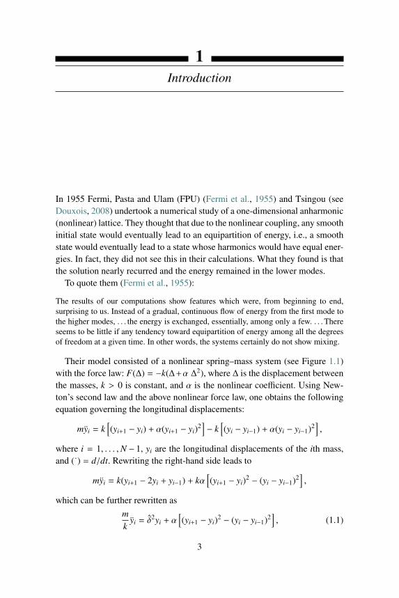
In 1955 Fermi, Pasta and Ulam (FPU) (Fermi et al., 1955) and Tsingou (seeDouxois, 2008) undertook a numerical study of a one-dimensional anharmonic(nonlinear) lattice. They thought that due to the nonlinear coupling, any smoothinitial state would eventually lead to an equipartition of energy, i.e., a smoothstate would eventually lead to a state whose harmonics would have equal ener-gies. In fact, they did not see this in their calculations. What they found is thatthe solution nearly recurred and the energy remained in the lower modes.
To quote them (Fermi et al., 1955):
The results of our computations show features which were, from beginning to end,surprising to us. Instead of a gradual, continuous flow of energy from the first mode tothe higher modes, . . . the energy is exchanged, essentially, among only a few. . . . Thereseems to be little if any tendency toward equipartition of energy among all the degreesof freedom at a given time. In other words, the systems certainly do not show mixing.
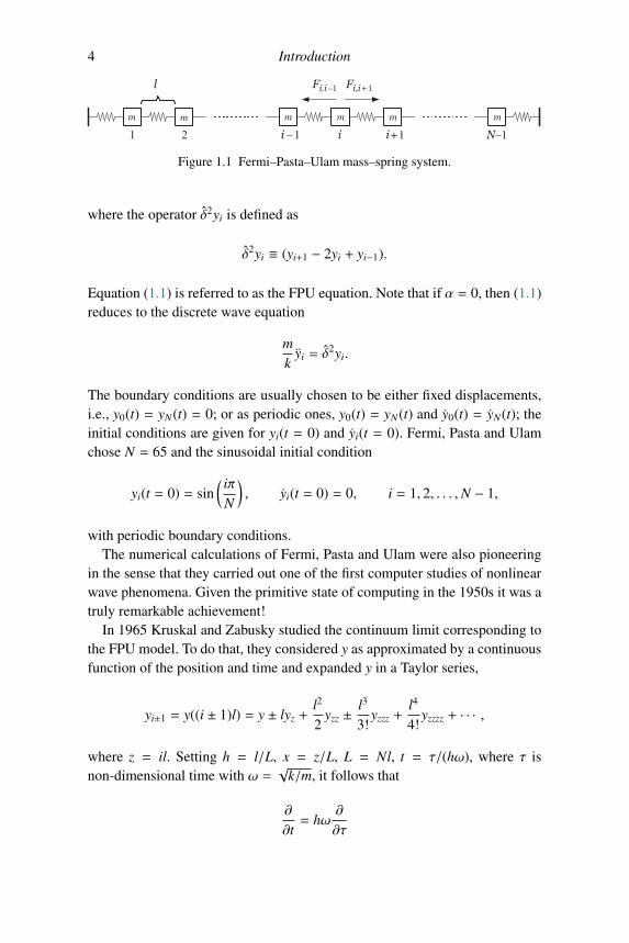
Their model consisted of a nonlinear spring–mass system (see Figure 1.1)with the force law: F(Δ) = −k(Δ+α Δ2), where Δ is the displacement betweenthe masses, k > 0 is constant, and α is the nonlinear coefficient. Using New-ton’s second law and the above nonlinear force law, one obtains the followingequation governing the longitudinal displacements:
myi = k[(yi+1 − yi) + α(yi+1 − yi)
2]− k[(yi − yi−1) + α(yi − yi−1)2
],
where i = 1, . . . ,N − 1, yi are the longitudinal displacements of the ith mass,and (˙) = d/dt. Rewriting the right-hand side leads to
myi = k(yi+1 − 2yi + yi−1) + kα[(yi+1 − yi)
2 − (yi − yi−1)2],
which can be further rewritten as
mk
yi = δ2yi + α
[(yi+1 − yi)
2 − (yi − yi−1)2], (1.1)
3
4 Introduction
i – 11 2 i i + 1 N–1
l
m mmmmm
Fi,i –1 Fi,i + 1
Figure 1.1 Fermi–Pasta–Ulam mass–spring system.
where the operator δ2yi is defined as
δ2yi ≡ (yi+1 − 2yi + yi−1).
Equation (1.1) is referred to as the FPU equation. Note that if α = 0, then (1.1)reduces to the discrete wave equation
mk
yi = δ2yi.
The boundary conditions are usually chosen to be either fixed displacements,i.e., y0(t) = yN(t) = 0; or as periodic ones, y0(t) = yN(t) and y0(t) = yN(t); theinitial conditions are given for yi(t = 0) and yi(t = 0). Fermi, Pasta and Ulamchose N = 65 and the sinusoidal initial condition
yi(t = 0) = sin( iπ
N
), yi(t = 0) = 0, i = 1, 2, . . . ,N − 1,
with periodic boundary conditions.The numerical calculations of Fermi, Pasta and Ulam were also pioneering
in the sense that they carried out one of the first computer studies of nonlinearwave phenomena. Given the primitive state of computing in the 1950s it was atruly remarkable achievement!
In 1965 Kruskal and Zabusky studied the continuum limit corresponding tothe FPU model. To do that, they considered y as approximated by a continuousfunction of the position and time and expanded y in a Taylor series,
yi±1 = y((i ± 1)l) = y ± lyz +l2
2yzz ± l3
3!yzzz +
l4
4!yzzzz + · · · ,
where z = il. Setting h = l/L, x = z/L, L = Nl, t = τ/(hω), where τ isnon-dimensional time with ω =
√k/m, it follows that
∂
∂t= hω
∂
∂τ
Introduction 5
and using the Taylor series on (1.1) leads to the continuous equation
h2yττ = h2yxx +h4
12yxxxx+α
⎡⎢⎢⎢⎢⎢⎣(hyx +h2
2yxx + . . .
)2−(hyx − h2
2yxx + . . .
)2⎤⎥⎥⎥⎥⎥⎦ .Hence, to leading order, the continuous limit is given by
yττ = yxx +h2
12yxxxx + εyxyxx + · · · , (1.2)
where ε = 2αh and the higher-order terms are neglected. This equation wasderived by Boussinesq in the context of shallow-water waves in 1871 and 1872(Boussinesq, 1871, 1872)!
There are four cases to consider:(a) When h2 � 1 and |ε| � 1 (read as h2 and |ε| are both much less than 1),
both the nonlinear term and higher-order derivative term (referred to as thedispersive term) are negligible. Then equation (1.2) reduces to the linearwave equation
yττ = yxx.
(b) In the small-amplitude limit where h2/12 � |ε| (or where α → 0 in theFPU model), the nonlinear term is negligible and the correction to (1.2) isgoverned by the higher-order linear dispersive wave equation
yττ = yxx +h2
12yxxxx.
(c) If h2/12 � |ε|, then the yxxxx term is negligible and (1.2) yields
yττ = yxx + εyxyxx,
which has, as can be shown from further analysis or indicated by numer-ical simulation, breaking or multi-valued solutions in finite time. Whenbreaking occurs one must use (1.2) as a more physical model.
(d) In the case of “maximal balance” where h2/12 ≈ |ε| � 1, the waveequation is governed by a different equation.
This case of maximal balance is the most interesting case and we will nowanalyze it in detail.
Let us look for a solution y of the form1
y ∼ Φ(X,T ; ε), X = x − τ, T =ετ
2.
1 Later in the book we will see “why”.
6 Introduction
It follows that
∂
∂τ= − ∂
∂X+ε
2∂
∂T,
∂2
∂τ2=
(∂
∂τ
)2=
∂2
∂X2− ε ∂
∂X∂T+ε2
4∂2
∂T 2,
∂
∂x=
∂
∂X.
Substituting these relations into the continuum limit, (1.2) yields[∂2Φ
∂X2− ε ∂Φ
∂X∂T+ε2
4∂2Φ
∂T 2
]=∂2Φ
∂X2+
h2
12∂4Φ
∂X4+ ε
∂Φ
∂X∂2Φ
∂X2.
Calling u = ∂Φ/∂X and dropping the O(ε2) terms, leads to the equation studiedby Zabusky and Kruskal (1965) and Kruskal (1965)
uT + uuX + δ2uXXX = 0, (1.3)
where δ2 = h2/12ε and u(X, 0) is the given initial condition. It is importantto note that (1.3) is the well-known (nonlinear) Korteweg–de Vries (KdV)equation. It should be remarked that Boussinesq derived (1.3) and otherapproximate long-wave equations for water waves [e.g., (1.2)] (Boussinesq,1871, 1872, 1877). Korteweg and de Vries investigated (1.3) in consider-able detail and found periodic “cnoidal” wave solutions in the context oflong (or shallow) water waves (Korteweg and de Vries, 1895). Before theearly 1960s, the KdV equation was primarily of interest only to researchersstudying water waves. The KdV equation was not of wide interest to mathe-maticians during the first half of the twentieth century, since most studies atthe time tended to concentrate on linear second-order equations, whereas (1.3)is nonlinear and third order.
Kruskal and Zabusky considered the KdV equation (1.3) with periodic initialvalues. They initially took δ2 small with u(X, 0) = cos(πX). When δ = 0 onegets the so-called inviscid Burgers equation,
uT + uuX = 0,
which leads to breaking or a multi-valued solution or shock formation in finitetime. The inviscid Burgers equation is discussed further in Chapter 2.
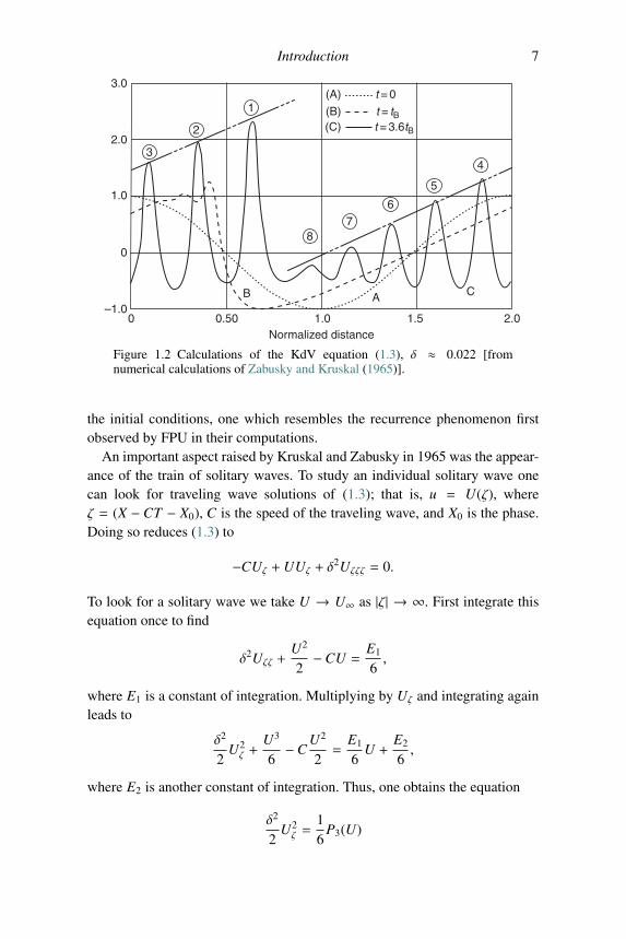
When δ2 � 1, a sharp gradient appears at a finite time, which we denoteby t = tB, together with “wiggles” (see the dashed line in Figure 1.2). Whent � tB, the solution develops many oscillations that eventually separate into atrain of solitary-type waves. Each solitary wave is localized in space (see thesolid line in Figure 1.2). Subsequently, under further propagation, the solitarywaves interact and the solution eventually returns to a state that is similar to
Introduction 7
3.0
2.03
1.0
0
–1.00 0.50 1.0 1.5 2.0
Normalized distance
AB C
2
1(A) t = 0
(B) t = tB(C) t = 3.6tB
7
6
5
4
8
Figure 1.2 Calculations of the KdV equation (1.3), δ ≈ 0.022 [fromnumerical calculations of Zabusky and Kruskal (1965)].
the initial conditions, one which resembles the recurrence phenomenon firstobserved by FPU in their computations.
An important aspect raised by Kruskal and Zabusky in 1965 was the appear-ance of the train of solitary waves. To study an individual solitary wave onecan look for traveling wave solutions of (1.3); that is, u = U(ζ), whereζ = (X − CT − X0), C is the speed of the traveling wave, and X0 is the phase.Doing so reduces (1.3) to
−CUζ + UUζ + δ2Uζζζ = 0.
To look for a solitary wave we take U → U∞ as |ζ | → ∞. First integrate thisequation once to find
δ2Uζζ +U2
2−CU =
E1
6,
where E1 is a constant of integration. Multiplying by Uζ and integrating againleads to
δ2
2U2ζ +
U3
6−C
U2
2=
E1
6U +
E2
6,
where E2 is another constant of integration. Thus, one obtains the equation
δ2
2U2ζ =
16
P3(U)
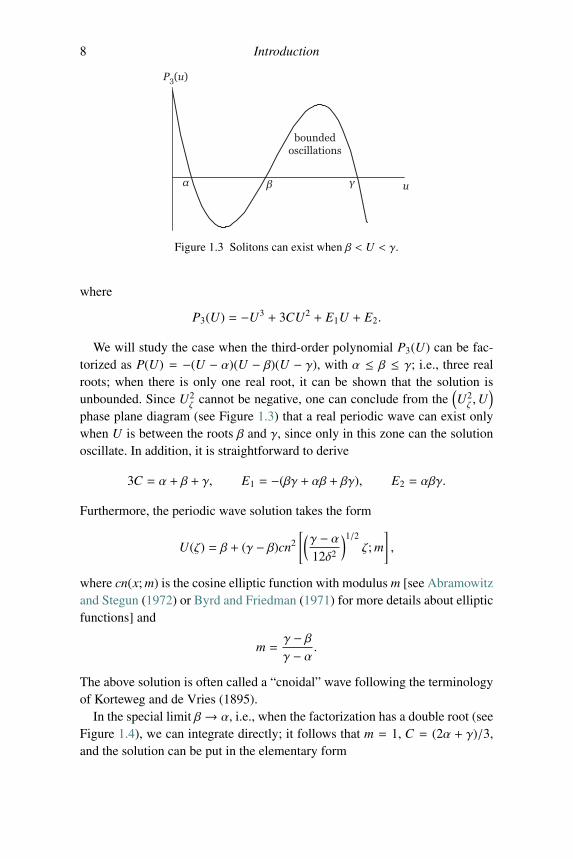
8 Introduction
u
P3(u)
boundedoscillations
α β γ
Figure 1.3 Solitons can exist when β < U < γ.
where
P3(U) = −U3 + 3CU2 + E1U + E2.
We will study the case when the third-order polynomial P3(U) can be fac-torized as P(U) = −(U − α)(U − β)(U − γ), with α ≤ β ≤ γ; i.e., three realroots; when there is only one real root, it can be shown that the solution isunbounded. Since U2
ζ cannot be negative, one can conclude from the(U2ζ ,U)
phase plane diagram (see Figure 1.3) that a real periodic wave can exist onlywhen U is between the roots β and γ, since only in this zone can the solutionoscillate. In addition, it is straightforward to derive
3C = α + β + γ, E1 = −(βγ + αβ + βγ), E2 = αβγ.
Furthermore, the periodic wave solution takes the form
U(ζ) = β + (γ − β)cn2
[(γ − α12δ2
)1/2ζ; m
],
where cn(x; m) is the cosine elliptic function with modulus m [see Abramowitzand Stegun (1972) or Byrd and Friedman (1971) for more details about ellipticfunctions] and
m =γ − βγ − α.
The above solution is often called a “cnoidal” wave following the terminologyof Korteweg and de Vries (1895).
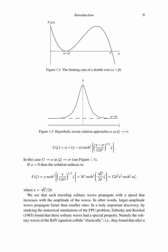
In the special limit β→ α, i.e., when the factorization has a double root (seeFigure 1.4), we can integrate directly; it follows that m = 1, C = (2α + γ)/3,and the solution can be put in the elementary form
Introduction 9
u
P3(u)
α = β γ
Figure 1.4 The limiting case of a double root (α = β).
u
u→α
ζ
Figure 1.5 Hyperbolic secant solution approaches α as |ζ| → ∞.
U(ζ) = α + (γ − α) sech2
[(γ − α12δ2
)1/2ζ
].
In this case U → α as |ζ | → ∞ (see Figure 1.5).If α = 0 then the solution reduces to
U(ζ) = γ sech2
[(γ
12δ2
)1/2ζ
]= 3C sech2
⎛⎜⎜⎜⎜⎝ √C2δ
ζ
⎞⎟⎟⎟⎟⎠ = 12δ2κ2 sech2 κζ,
where κ =√
C/2δ.We see that such traveling solitary waves propagate with a speed that
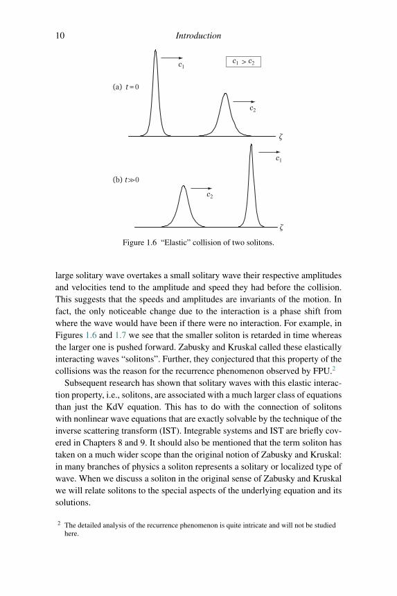
increases with the amplitude of the waves. In other words, larger-amplitudewaves propagate faster than smaller ones. In a truly important discovery, bystudying the numerical simulations of the FPU problem, Zabusky and Kruskal(1965) found that these solitary waves had a special property. Namely the soli-tary waves of the KdV equation collide “elastically”; i.e., they found that after a
10 Introduction
ζ
(a) t = 0
c1
c2
c1 > c2
c1
c2
(b) tà0
ζ
Figure 1.6 “Elastic” collision of two solitons.
large solitary wave overtakes a small solitary wave their respective amplitudesand velocities tend to the amplitude and speed they had before the collision.This suggests that the speeds and amplitudes are invariants of the motion. Infact, the only noticeable change due to the interaction is a phase shift fromwhere the wave would have been if there were no interaction. For example, inFigures 1.6 and 1.7 we see that the smaller soliton is retarded in time whereasthe larger one is pushed forward. Zabusky and Kruskal called these elasticallyinteracting waves “solitons”. Further, they conjectured that this property of thecollisions was the reason for the recurrence phenomenon observed by FPU.2
Subsequent research has shown that solitary waves with this elastic interac-tion property, i.e., solitons, are associated with a much larger class of equationsthan just the KdV equation. This has to do with the connection of solitonswith nonlinear wave equations that are exactly solvable by the technique of theinverse scattering transform (IST). Integrable systems and IST are briefly cov-ered in Chapters 8 and 9. It should also be mentioned that the term soliton hastaken on a much wider scope than the original notion of Zabusky and Kruskal:in many branches of physics a soliton represents a solitary or localized type ofwave. When we discuss a soliton in the original sense of Zabusky and Kruskalwe will relate solitons to the special aspects of the underlying equation and itssolutions.
2 The detailed analysis of the recurrence phenomenon is quite intricate and will not be studiedhere.
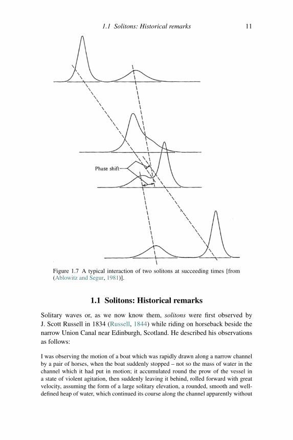
1.1 Solitons: Historical remarks 11
Figure 1.7 A typical interaction of two solitons at succeeding times [from(Ablowitz and Segur, 1981)].
1.1 Solitons: Historical remarks
Solitary waves or, as we now know them, solitons were first observed byJ. Scott Russell in 1834 (Russell, 1844) while riding on horseback beside thenarrow Union Canal near Edinburgh, Scotland. He described his observationsas follows:
I was observing the motion of a boat which was rapidly drawn along a narrow channelby a pair of horses, when the boat suddenly stopped – not so the mass of water in thechannel which it had put in motion; it accumulated round the prow of the vessel ina state of violent agitation, then suddenly leaving it behind, rolled forward with greatvelocity, assuming the form of a large solitary elevation, a rounded, smooth and well-defined heap of water, which continued its course along the channel apparently without
12 Introduction
change of form or diminution of speed. I followed it on horseback, and overtook itstill rolling on at a rate of some eight or nine miles an hour, preserving its originalfigure some thirty feet long and a foot to a foot and a half in height. Its height graduallydiminished, and after a chase of one or two miles I lost it in the windings of the channel.Such, in the month of August 1834, was my first chance interview with that rare andbeautiful phenomenon which I have called the Wave of Translation . . .
Subsequently, Russell carried out experiments in a laboratory wave tank tostudy this phenomenon more carefully. He later called the solitary wave theGreat Primary Wave of Translation. Russell’s work on the wave of translationwas the first detailed study of these localized waves. Included among Russell’sresults are the following:• he observed solitary waves, which are long, shallow-water waves of perma-
nent form, hence he deduced that they exist;• the speed of propagation, c, of a solitary wave in a channel of uniform depth
h is given by c2 = c20(1 + A/h), c2
0 = gh, where A is the maximum ampli-tude of the wave, h is the mean level above a rigid bottom and g is thegravitational constant.Russell’s results provoked considerable discussion and controversy. Airy, a
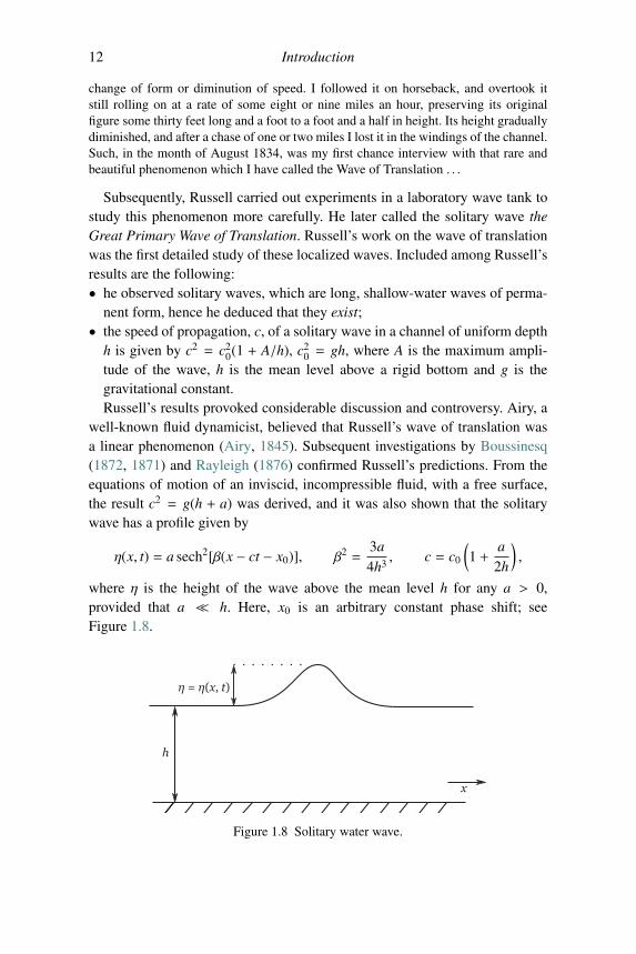
well-known fluid dynamicist, believed that Russell’s wave of translation wasa linear phenomenon (Airy, 1845). Subsequent investigations by Boussinesq(1872, 1871) and Rayleigh (1876) confirmed Russell’s predictions. From theequations of motion of an inviscid, incompressible fluid, with a free surface,the result c2 = g(h + a) was derived, and it was also shown that the solitarywave has a profile given by
η(x, t) = a sech2[β(x − ct − x0)], β2 =3a4h3
, c = c0
(1 +
a2h
),
where η is the height of the wave above the mean level h for any a > 0,provided that a � h. Here, x0 is an arbitrary constant phase shift; seeFigure 1.8.
h
η = η(x, t)
x
Figure 1.8 Solitary water wave.
1.1 Solitons: Historical remarks 13
Understanding was further advanced by Korteweg and de Vries (1895).They derived a nonlinear evolution equation governing long, one-dimensional,small-amplitude, surface gravity waves propagating in shallow water, nowknown as the KdV equation (in dimensional form):
1c0
∂η
∂t+∂η
∂x+
32hη∂η
∂x+
h2
2
(13− T
)∂3η
∂x3= 0, (1.4)
where η is the surface elevation of the wave, h is the equilibrium level, g isthe gravitational constant of acceleration, c0 =
√gh, T = T/ρgh2, T is the
surface tension and ρ is the density (the terms “long” and “small” are meant incomparison to the depth of the channel, see Chapter 5).
Korteweg and de Vries showed (1.4) has traveling wave solutions, includ-ing periodic Jacobian elliptic (cosine) function solutions that they termed“cnoidal” functions, and a special case of a cnoidal function (when the ellip-tic modulus tends to unity) is a solitary wave solution. Equation (1.4) may bebrought into non-dimensional form by making the transformation
σ =13− T , t′ = βt, x′ =
1h
(x − c0t),
β =c0σ
2h, η = 2hσu.
Hence, we obtain (after dropping the primes)
ut + 6uux + uxxx = 0. (1.5)
This dimensionless equation is usually referred to as the KdV equation. Wenote that any constant coefficient may be placed in front of any of the threeterms by a suitable scaling of the independent and dependent variables.
Despite this derivation of the KdV equation in 1895, it was not until 1960that new applications of it were discovered. Gardner and Morikawa (1960)rediscovered the KdV equation in the study of collision-free hydromagneticwaves. Subsequently the KdV equation has arisen in a number of other phys-ical contexts, including stratified internal waves, ion-acoustic waves, plasmaphysics, lattice dynamics, etc. Actually the KdV equation is “universal” in thesense that it always arises when the governing equation has weak quadraticnonlinearity and weak dispersion. See also Benney and Luke (1964), Benney(1966a,b), Gardner and Su (1969) and Taniuti and Wei (1968).
As mentioned above, it has been known since the work of Korteweg and deVries that the KdV equation (1.5) possesses the solitary wave solution
u(x, t) = 2κ2 sech2{κ(x − 4κ2t − δ0)
}, (1.6)
14 Introduction
where κ and δ0 are constants. Note that the velocity of this wave, 4κ2, is pro-portional to the amplitude, 2κ2; therefore taller waves travel faster than shorterones. In dimensional variables the soliton with κ = kh, δ0 = 0, takes the form
η = 2Ah sech2[k(x − c0
(1 +
A2
)t)], A = 2σk2,
which agrees with Russell’s observations mentioned above.As discussed earlier, Zabusky and Kruskal (1965) discovered that these soli-
tary wave solutions have the remarkable property that the interaction of twosolitary wave solutions is elastic, and called the waves solitons.
Finally, we mention that there are numerous useful texts that discuss non-linear waves in the context of physically significant problems. The readeris encouraged to consult these references: Phillips (1977); Rabinovich andTrubetskov (1989); Whitham (1974); Lighthill (1978); Infeld and Rowlands(2000); Ostrovsky and Potapov (1986); see also the essay by Miles (1981).
Exercises
1.1 Following the methods described in this chapter, derive a generalizedKdV equation from the FPU problem when the spring force law isgiven by
F(Δ) = −k(Δ + αΔ3),
where Δ is the displacement between masses and k, α are constants.1.2 Given the modified KdV (mKdV) equation
ut + 6u2ux + uxxx = 0,
reduce the problem to an ODE by investigating traveling wave solutionsof the form: u = U(x − ct).(a) Express the bounded periodic solution in terms of Jacobi elliptic
functions.(b) Find all bounded solitary wave solutions.
1.3 Consider the sine–Gordon (SG) equation given by
utt − uxx + sin u = 0.
(a) Use the transformation u = U(x−ct), where c is a constant, to reducethe SG equation to a second-order ODE.
(b) Find a first-order ODE by integrating once.
Exercises 15
(c) Make the transformation U = 2 tan−1 w (inverse tan function), andsolve the equation for w to find all bounded, real periodic solutionsfor w and therefore U. Express the solution in terms of Jacobi ellipticfunctions. (Hint: See Chapter 4.)
(d) Use the above to find all bounded wave solutions U that tend to zeroat −∞ and 2π at +∞. These are called kink solutions; they turn outto be solitons.
1.4 Consider the KdV equation
ut + 6uux + uxxx = 0.
(a) Make the transformation x→ klx, t → kmt, u→ knu, k � 0, and findl, m, n so that the KdV equation is invariant under the transformation.
(b) Make the transformation u = t−2/3 f (v), v = xt−1/3, f = 2(log F)′′.Find an equation for the similarity solution f and an equation for F;then obtain a rational solution to the KdV equation. (See Section 3.2for a discussion of self-similar/similarity solutions.)
1.5 Find the bounded traveling wave solution to the generalized KdV
ut + (n + 1)(n + 2)unux + uxxx = 0
where n = 1, 2, . . ..1.6 Consider the modified KdV (mKdV) equation
ut − 6u2ux + uxxx = 0.
(a) Make the transformation x → alx, t → amt, u → anu and find l, m,n, so that the equation is invariant under the transformation.
(b) Introduce u(x, t) = (3t)−1/3 f (ξ), ξ = x(3t)−1/3 to reduce the mKdVequation to the following ODE
f ′′ = ξ f + 2 f 3 + α
where α is constant. The equation for f is called the second Painleveequation, cf. Ablowitz and Segur (1981).
1.7 Show that a solitary wave solution of the Boussinesq equation,
utt − uxx + 3(u2)xx − uxxxx = 0,
is u(x, t) = a sech2[b(x − ct) + d], for suitable relations between theconstants a, b, c, and d. Verify that the Boussinesq solitary wave canpropagate in either direction.
1.8 Find the bounded traveling wave solution to the equation
utt = uxx + uxuxx + uxxxx.
16 Introduction
Hint: Set ξ = x − ct, integrate twice with respect to ξ, and use uξ = q(u)to solve the resulting equation.
1.9 Consider the sine–Gordon equation
uxx − utt = sin u.
(a) Using the transformation χ = γ(x − vt), τ = γ(t − vx) write theequation in terms of the new coordinates χ, τ; find γ in terms of v,−1 < v < 1 so that the equation is invariant under the transformation.
(b) Consider the transformation ξ = (x + t)/2, η = (x − t)/2. Find theequation in terms of the new coordinates ξ, η. Show that this equationhas a self-similar solution of the form u(ξ, η) = f (z), z = ξη. Thenfind an equation for w = exp(i f ). The equation for w is related to thethird Painleve equation, cf. Ablowitz and Segur (1981). (See Section3.2 for a discussion of self-similar/similarity solutions.)
1.10 Seek a similarity solution of the Klein–Gordon equation,
utt − uxx = u3,
in the form u(x, t) = tm f (xtn) for suitable values of m and n. Show thatf (z), z = x/t satisfies the equation (z2 − 1) f ′′ + 4z f ′ + 2 f = f 3. (SeeSection 3.2 for a discussion of self-similar/similarity solutions.)
2Linear and nonlinear wave equations
In Chapter 1 we saw how the KdV equation can be derived from the FPUproblem. We also mentioned that the KdV equation was originally derived forweakly nonlinear water waves in the limit of long or shallow water waves.Researchers have subsequently found that the KdV equation is “universal” inthe sense that it arises whenever we have a weakly dispersive and a weaklyquadratic nonlinear system. Thus the KdV equation has also been derived fromother physical models, such as internal waves, ocean waves, plasma physics,waves in elastic media, etc. In later chapters we will analyze water waves indepth, but first we will discuss some basic aspects of waves.
Broadly speaking, the study of wave propagation is the study of how signalsor disturbances or, more generally, information is transmitted (cf. Bleistein,1984). In this chapter we begin with a study of “dispersive waves” and wewill introduce the notion of phase and group velocity. We will then brieflydiscuss: the linear wave equation, the concept of characteristics, shock wavesin scalar first-order partial differential equations (PDEs), traveling waves of theviscous Burgers equation, classification of second-order quasilinear PDEs, andthe concept of the well-posedness of PDEs.
2.1 Fourier transform method
Consider a PDE in evolution form, first order in time, and in one spatialdimension,
ut = F[u, ux, uxx, . . . ],
where F is, say, a polynomial function of its arguments. We will consider theinitial value problem on |x| < ∞ and assume u → 0 sufficiently rapidly as|x| → ∞ with u(x, 0) = u0(x) given. To begin with, suppose we consider thelinear homogeneous case, i.e.,
17
18 Linear and nonlinear wave equations
ut =
N∑j=0
a j(x, t)u jx,
where ujx ≡ ∂ ju/∂x j and a j(x, t) are prescribed coefficients. When the a j areconstants,
ut =
N∑j=0
a ju jx, (2.1)
and u0(x) decays fast enough, then we can use the method of Fourier transformsto solve this equation. Before we do that, however, let us recall some basic factsabout Fourier transforms (cf. Ablowitz and Fokas, 2003).
The function u(x, t) can be expressed using the (spatial) Fourier transform as
u(x, t) =1
2π
∫b(k, t)eikx dk, (2.2)
where it is assumed that u is smooth and |u| → 0 as |x| → ∞ sufficientlyrapidly; also, unless otherwise specified,
∫represents an integral from −∞ to
+∞ in this chapter. For our purposes it suffices to require that u ∈ L1⋂
L2,meaning that
∫ |u| dx and∫ |u|2 dx are both finite. Substituting (2.2) into (2.1),
assuming the interchange of derivatives and integral, leads to∫eikx{bt − b
N∑j=0
(ik) ja j
}dk = 0.
It follows that
bt = bN∑
j=0
(ik) ja j,
or that
bt = −iω(k)b,
with
−iω(k) =N∑
j=0
(ik) ja j. (2.3)
We call ω(k), which we assume is real, the dispersion relation correspondingto (2.1). For example, if N = 3, then ω(k) = ia0 − ka1 − ik2a2 + k3a3 and ω(k)is real if a1, a3 are real and a0, a2 are pure imaginary. We can solve this ODEto get
b(k, t) = b0(k)e−iω(k)t,
2.2 Terminology: Dispersive and non-dispersive equations 19
where b0(k) ≡ b(k, 0). From this one obtains
u(x, t) =1
2π
∫b0(k)ei[kx−ω(k)t] dk.
Hence b0(k) plays the role of a weight function, which depends on the initialconditions according to the inverse Fourier transform:
b0(k) =∫
u(x, 0)e−ikx dx.
Strictly speaking, we now have an “algorithm” in terms of integrals forsolving our problem for u(x, t).
Note that, in retrospect, we can also obtain this relation by substituting
u(x, t) =1
2π
∫b0(k)ei[kx−ω(k)t] dk
into the PDE.There is, in fact, an alternative method for obtaining the dispersion relation.
It is based on the observation that in this case one can substitute us = ei[kx−ω(k)t]
into the PDE and replace the time and spatial derivatives by
∂t → −iω, ∂x → ik.
Then (2.3) follows from (2.1) directly.
2.2 Terminology: Dispersive and non-dispersive equations
Let us define and then explain the terminology that is frequently used in con-junction with these wave problems and Fourier transforms: k is usually calledthe wavenumber, ω is the frequency, k and ω real, and θ ≡ kx − ω(k)t is thephase in the exponent or simply the phase.
The temporal period (or period for short) is denoted by
T ≡ 2πω.
The meaning of the period is that whenever t → t + nT , where n is an inte-ger, then the phase remains the same modulo 2π and therefore eiθ remainsunchanged. Similarly, we call λ = 2π/k the wavelength and note that when-ever x → x + nλ the phase remains the same modulo 2π and therefore eiθ
remains unchanged. Furthermore, we call
c(k) ≡ ω(k)k
20 Linear and nonlinear wave equations
the phase velocity, since θ = k(x − c(k)t). There is also the notion of groupvelocity vg(k) ≡ ω′(k); i.e., the speed of a slowly varying group of waves. Wewill discuss its importance later.
An equation in one space and one time dimension is said to be dispersivewhenω(k) is real-valued andω′′(k) � 0. The meaning of dispersion will be fur-ther elucidated when we discuss the long time asymptotics of these equations.Consider the first-order linear equation
ut − a1ux = 0, (2.4)
where a1 � 0, real and constant. We see that
−iω = ika1,
which gives the linear dispersion relation
ω(k) = −a1k.
In this case ω′′(k) ≡ 0, which means the PDE is non-dispersive.Now let us look at the first-order constant coefficient equation (2.1). In this
case the dispersion relation (2.3) shows that if all the a j are real, then ω is realif and only if all the even powers of k (or even values of the index j) vanish;i.e., aj = 0 for j = 2, 4, 6, . . . . In that case it follows from (2.3) that ω(k) is anodd function of k, in which case the dispersion relation takes the general form
ω(k) = −N∑
j=0
(−1) ja2 j+1k2 j+1.
A further example is the linearized KdV equation given by
ut + uxxx = 0, (2.5)
i.e., (1.5) without the nonlinear term. By substituting us = ei[kx−ω(k)t] oneobtains its dispersion relation,
ω(k) = −k3.
Thus ω is real and ω′′ = −6k � 0, which means that this is a dispersiveequation.
We can use Fourier transforms to solve this equation. As indicated above,using the Fourier transform, u(x, t) can be expressed as
u(x, t) =1
2π
∫b(k, t)eikx dk,
2.2 Terminology: Dispersive and non-dispersive equations 21
and for the linearized KdV equation (2.5) one finds that bt = ik3b hence
u(x, t) =1
2π
∫b0(k)ei(kx+k3t) dk.
However, by itself this is not a particularly insightful solution, since one cannotevaluate this integral explicitly. Often having an integral formula alone doesnot give useful qualitative information. Similarly, we usually cannot explicitlyevaluate the integrals corresponding to most linear dispersive equations. This isexactly the place where asymptotics of integrals plays an extremely importantrole: it will allow us to approximate the integrals with simple, understandableexpressions. This will be a recurring theme in this book: namely, analyticalmethods can yield solutions that are inconvenient or uninformative and asymp-totics can be used to obtain valuable information about these problems. Laterwe will briefly discuss the long-time asymptotic analysis of the linearized KdVequation.
In so far as we are dealing with dispersive equations, we have seen thatrequiring ω(k) to be real implies that ω(k) is odd. If in addition, u(x, t) is real,this knowledge can be encoded into b0(k) as follows. We have that
u∗(x, t) =1
2π
∫b∗0(k)e−i[kx−ω(k)t] dk,
where u∗ denotes the complex conjugate of u. Calling k′ = −k yields
u∗(x, t) = − 12π
∫ −∞
∞b∗0(−k′)e−i[−k′x−ω(−k′)t] dk′
=1
2π
∫ ∞
−∞b∗0(−k′)e−i[−k′x−ω(−k′)t] dk′.
Then if we require that u is real-valued then u(x, t) = u∗(x, t). In addition,ω(−k′) = −ω(k). Combined, one obtains that
12π
∫b0(k)ei[kx−ω(k)t] dk =
12π
∫b∗0(−k′)ei[k′x−ω(k′)t] dk′.
This identity is satisfied for all (x, t) if and only if
b∗0(k) = b0(−k).
Note that we cannot apply the Fourier transform method for the nonlinearproblem, sometimes called the inviscid Burgers equation,
ut + uux = 0,
because of the nonlinear product. We study the solution of this equation byusing the method of characteristics; this is briefly discussed later in this chapter.
22 Linear and nonlinear wave equations
We also note that for some problems, us = exp(i(kx −ω(k)t)) yields an ω(k)that is not purely real. For example, for the so-called heat or diffusion equation
ut = uxx,
we find ω(k) = −ik2. The Fourier transform method works as before giving
u(x, t) =1
2π
∫ ∞
−∞b0(k)eikx−k2t dk.
We see that the solution decays, i.e., the solution diffuses with increasing t.
2.3 Parseval’s theorem
The L2-norm of a function f (x) is defined by
‖ f ‖22 ≡∫| f (x)|2 dx.
Let f (k) be the Fourier transform of f (x). Parseval’s theorem [see e.g.,Ablowitz and Fokas (2003)] states that
‖ f (x)‖22 =1
2π‖ f (k)‖22.
In many cases the L2-norm of the solutions of PDEs has the meaning of energy(i.e., is proportional to the energy in physical units). The physical meaningassociated with Parseval’s relation is that the energy in physical space is equalto the energy in frequency (or sometimes called spectral or Fourier) space.Moreover, we know that when ω is real-valued then∫
|u(x, t)|2 dx =1
2π
∫|b0(k)|2 dk = constant.
Hence, it follows from Parseval’s theorem that energy is conserved in lin-ear dispersive equations. While it is possible to prove this result using directintegration methods, we get it “for free” in linear PDEs using Parseval’stheorem.
2.4 Conservation laws
We saw above how Parseval’s theorem is used to prove energy conservation.However, there may be other conserved quantities. These often play a veryuseful role in the analysis of problems, as we will see later.
2.5 Multidimensional dispersive equations 23
A conservation law (or relation) has the general form
∂
∂tT (x, t) +
∂
∂xF(x, t) = 0;
we call T the density of the conserved quantity, and F the flux. Let us integratethis relation from x = −∞ to x = ∞:
∂
∂t
∫T dx + F(x, t)
∣∣∣∣∣x→+∞x→−∞
= 0.
The second term is zero, since we assume that F decays at infinity, whichleads to
∂
∂t
∫T dx = 0,
i.e.,∫
T dx = constant.For example, let us study the conservation laws for the linearized KdV
equation:
ut + uxxx = 0.
This equation is already in the form of a conservation law, with T1 = u andF1 = uxx; that is,
∫u dx is conserved. This, however, is only one of many
conservation laws corresponding to (2.5). Another example is energy conser-vation. Using Parseval’s theorem, we have already proven that linear dispersiveequations with constant coefficients satisfy energy conservation. Since (2.5) issolvable by Fourier transforms we know from Parseval’s theorem that energyis conserved. An alternative way of seeing this is by multiplying (2.5) by u andintegrating with respect to x. It can be checked that this leads to
∂
∂t
(12
u2)+∂
∂x
(uuxx − 1
2u2
x
)= 0,
from which it follows that∫ |u|2 dx = constant.
2.5 Multidimensional dispersive equations
So far we have focused on dispersive equations in one spatial dimension. Themethod of Fourier transforms can be generalized to solve constant coefficientmultidimensional equations, where a typical solution takes the form:
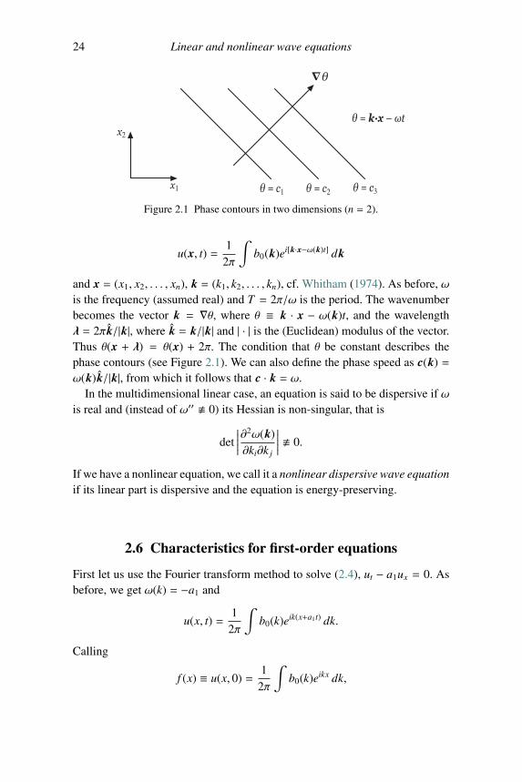
24 Linear and nonlinear wave equations
Figure 2.1 Phase contours in two dimensions (n = 2).
u(x, t) =1
2π
∫b0(k)ei[k·x−ω(k)t] dk
and x = (x1, x2, . . . , xn), k = (k1, k2, . . . , kn), cf. Whitham (1974). As before, ωis the frequency (assumed real) and T = 2π/ω is the period. The wavenumberbecomes the vector k = ∇θ, where θ ≡ k · x − ω(k)t, and the wavelengthλ = 2πk/|k|, where k = k/|k| and | · | is the (Euclidean) modulus of the vector.Thus θ(x + λ) = θ(x) + 2π. The condition that θ be constant describes thephase contours (see Figure 2.1). We can also define the phase speed as c(k) =ω(k)k/|k|, from which it follows that c · k = ω.
In the multidimensional linear case, an equation is said to be dispersive if ωis real and (instead of ω′′ � 0) its Hessian is non-singular, that is
det∣∣∣∣∣∂2ω(k)∂ki∂k j
∣∣∣∣∣ � 0.
If we have a nonlinear equation, we call it a nonlinear dispersive wave equationif its linear part is dispersive and the equation is energy-preserving.
2.6 Characteristics for first-order equations
First let us use the Fourier transform method to solve (2.4), ut − a1ux = 0. Asbefore, we get ω(k) = −a1 and
u(x, t) =1
2π
∫b0(k)eik(x+a1t) dk.
Calling
f (x) ≡ u(x, 0) =1
2π
∫b0(k)eikx dk,
2.6 Characteristics for first-order equations 25
we observe that u(x, t) = f (x + a1t). This solution can be checked directly bysubstitution into the PDE.
We can also solve (2.4) using the so-called method of characteristics. Wecan think of the left-hand side of (2.4) as a total derivative that is expandedaccording to the chain rule. That is,
dudt=∂u∂t+
dxdt∂u∂x= 0. (2.6)
It follows from (2.6) that du/dt = 0 along the curves dx/dt = −a1, or, saiddifferently, that u = c2, a constant, along the curves x + a1t = c1. Thus for theinitial value problem u(x, t = 0) = f (x), at any point x = ξ we can identifythe constant c2 with f (ξ) and c1 with ξ. Hence the solution to the initial valueproblem is given by
u = f (x + a1t).
Alternatively, from (2.4) and (2.6) (solving for du), we can write the abovein the succinct form
dt1=
dx−a1=
du0.
These equations imply that
t =−1a1
x +c1
a1, u = c2,
where c1 and c2 are constants. Hence
x + a1t = c1, u = c2.
For first-order PDEs the solution has one arbitrary function degree of freedomand the constants are related by this function. In this case c2 = g(c1), where gis an arbitrary function, leads to
u = g(x + a1t).
As above, suppose we specify the initial condition u(x, 0) = f (x). Then if wetake c1 = ξ, so that t = 0 corresponds to the point x = ξ on the initial data, thisthen implies that u(ξ, t) = g(ξ) = f (ξ); now in general, along ξ = x + a1t, thatagrees with the solution obtained by Fourier transforms. The meaning of ξ isthat of a characteristic curve (a line in this case) in the (x, t)-plane, along whichthe solution is non-unique; in other words, along a characteristic ξ, the solutioncan be specified arbitrarily. Moreover as we move from one characteristic, sayξ1, to another, say ξ2, the solution can change abruptly.
26 Linear and nonlinear wave equations
The method of characteristics also applies to quasilinear first-order equa-tions. For example, let us consider the inviscid Burgers equation mentionedearlier:
ut + uux = 0. (2.7)
From (2.7) we have that du/dt = 0 along the curves dx/dt = u, or, said differ-ently, that u = c2, a constant, along the curves x − ut = c1. Hence an implicitsolution is given by
u = f (x − ut).
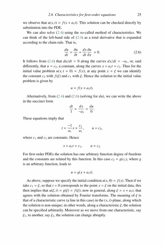
Alternatively, if we specify the initial condition u(x, 0) = f (x), with f (x) asmooth function of x, and we take c1 = ξ so that corresponding to t = 0 isa point x = ξ on the initial data, this then means that u(x, t) = f (ξ) alongx = ξ + f (ξ)t. The latter equation implies that ξ is a function of time, i.e., ξ =ξ(x, t), which in turn leads to the solution u = u(x, t). If we have a “hump-like”initial condition such as u(x, 0) = sech2 x then either points at the top of thecurve, e.g., the maximum, “move” faster than the points of lower amplitude andeventually break, or a multi-valued solution occurs. The breaking time followsfrom x = ξ + f (ξ)t. Taking the derivative of this equation yields ∂ξ/∂x = ξx
and ξt:
ξx =1
f ′(ξ)t + 1, ξt = − f (ξ)
f ′(ξ)t + 1(2.8)
and the breaking time is given by t = tB = 1/max(− f ′). This is the breakingtime, depicted in Figure 1.2, that is associated with the KdV equation (dashedline) in Chapter 1.
Thus the solution to (2.7) can be written in the form
u = u(ξ(x, t)).
Prior to the breaking time t = tB the solution is single valued. So we can verifythat the solution (2.8) satisfies the equation:
ut = u′(ξ)ξt
ux = u′(ξ)ξx
and using (2.7) and (2.8)
ut + uux = − f (ξ)f ′(ξ)t + 1
+f (ξ)
f ′(ξ)t + 1= 0.
In the exercises, other first-order equations are studied by the method ofcharacteristics.
2.7 Shock waves and the Rankine–Hugoniot conditions 27
u
x (a) (b) (c)
t = 0 t = tB t > tB
Figure 2.2 The solution of (2.7) at different times.
u
x
(a)
ξ = 0 ξ = xIxI xx = 0
(b)t
x = f(ξ)t + ξ
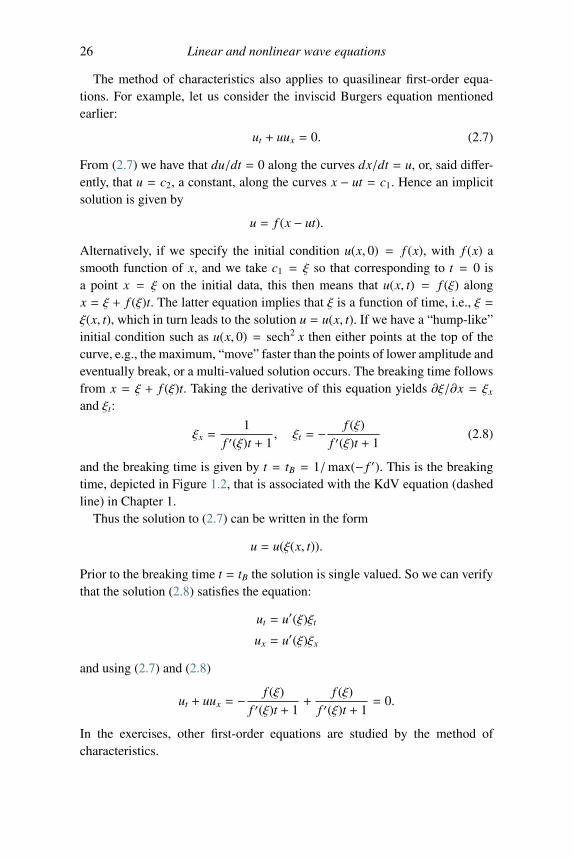
Figure 2.3 (a) A typical function u(ξ, 0) = f (ξ). (b) Characteristics associ-ated with points ξ = 0, ξ = xI that intersect at t = tB. The point xI is theinflection point of f (ξ).
In Figure 2.2 is shown a typical case and we can formally find the solu-tion for values t > tB ignoring the singularities and triple-valued solution.The value of time t, when characteristics first intersect, is denoted by tB – seeFigure 2.3.
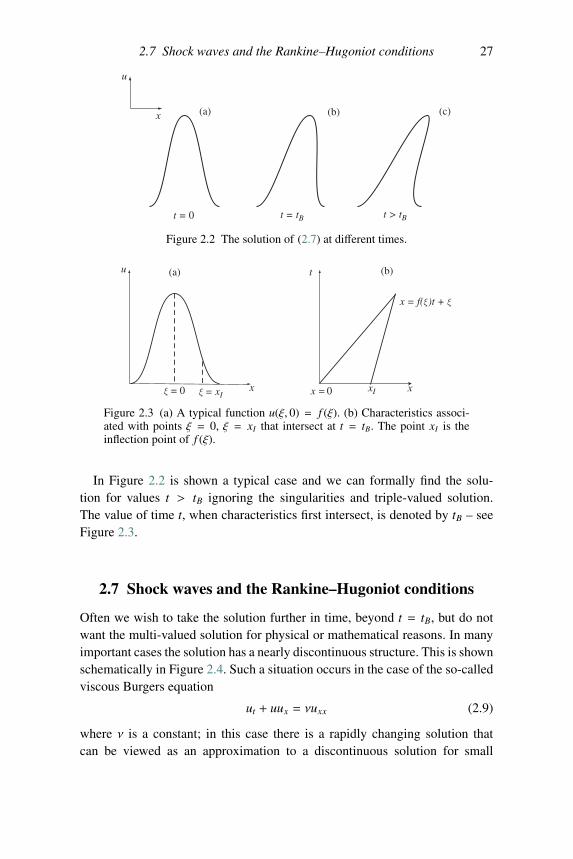
2.7 Shock waves and the Rankine–Hugoniot conditions
Often we wish to take the solution further in time, beyond t = tB, but do notwant the multi-valued solution for physical or mathematical reasons. In manyimportant cases the solution has a nearly discontinuous structure. This is shownschematically in Figure 2.4. Such a situation occurs in the case of the so-calledviscous Burgers equation
ut + uux = νuxx (2.9)
where ν is a constant; in this case there is a rapidly changing solution thatcan be viewed as an approximation to a discontinuous solution for small
28 Linear and nonlinear wave equations
u
x (a) (b) (c)
t = 0 t = tB t > tB
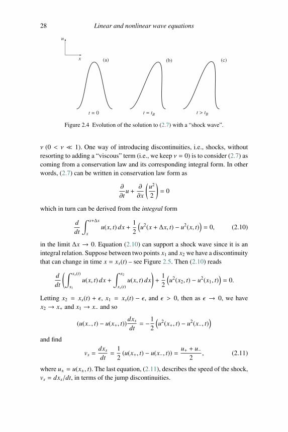
Figure 2.4 Evolution of the solution to (2.7) with a “shock wave”.
ν (0 < ν � 1). One way of introducing discontinuities, i.e., shocks, withoutresorting to adding a “viscous” term (i.e., we keep ν = 0) is to consider (2.7) ascoming from a conservation law and its corresponding integral form. In otherwords, (2.7) can be written in conservation law form as
∂
∂tu +
∂
∂x
(u2
2
)= 0
which in turn can be derived from the integral form
ddt
∫ x+Δx
xu(x, t) dx +
12
(u2(x + Δx, t) − u2(x, t)
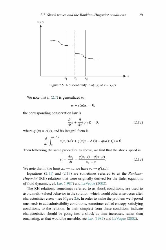
)= 0, (2.10)
in the limit Δx → 0. Equation (2.10) can support a shock wave since it is anintegral relation. Suppose between two points x1 and x2 we have a discontinuitythat can change in time x = xs(t) – see Figure 2.5. Then (2.10) reads
ddt
(∫ xs(t)
x1
u(x, t) dx +∫ x2
xs(t)u(x, t) dx
)+
12
(u2(x2, t) − u2(x1, t)
)= 0.
Letting x2 = xs(t) + ε, x1 = xs(t) − ε, and ε > 0, then as ε → 0, we havex2 → x+ and x1 → x− and so
(u(x−, t) − u(x+, t))dxs
dt= −1
2
(u2(x+, t) − u2(x−, t)
)and find
vs =dxs
dt=
12
(u(x+, t) − u(x−, t)) =u+ + u−
2, (2.11)
where u± = u(x±, t). The last equation, (2.11), describes the speed of the shock,vs = dxs/dt, in terms of the jump discontinuities.
2.7 Shock waves and the Rankine–Hugoniot conditions 29
u(x,t)
xx1 x2xs
Figure 2.5 A discontinuity in u(x, t) at x = xs(t).
We note that if (2.7) is generalized to
ut + c(u)ux = 0,
the corresponding conservation law is
∂
∂tu +
∂
∂x(q(u)) = 0, (2.12)
where q′(u) = c(u), and its integral form is
ddt
∫ x+Δx
xu(x, t) dx + q(u(x + Δx)) − q(u(x, t)) = 0.
Then following the same procedure as above, we find that the shock speed is
vs =dxs
dt=
q(x+, t) − q(x−, t)u+ − u−
. (2.13)
We note that in the limit x+ → x− we have vs → q′(x+).Equations (2.11) and (2.13) are sometimes referred to as the Rankine–
Hugoniot (RH) relations that were originally derived for the Euler equationsof fluid dynamics, cf. Lax (1987) and LeVeque (2002).
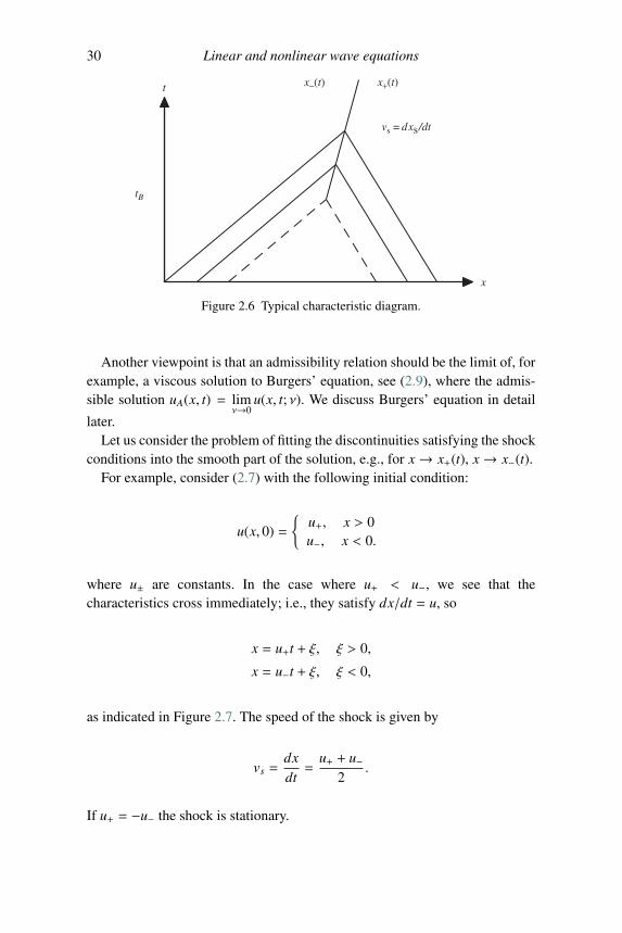
The RH relations, sometimes referred to as shock conditions, are used toavoid multi-valued behavior in the solution, which would otherwise occur aftercharacteristics cross – see Figure 2.6. In order to make the problem well-posedone needs to add admissibility conditions, sometimes called entropy-satisfyingconditions, to the relation. In their simplest form these conditions indicatecharacteristics should be going into a shock as time increases, rather thanemanating, as that would be unstable, see Lax (1987) and LeVeque (2002).
30 Linear and nonlinear wave equations
t
x
tB
x−(t) x+(t)
vs = d xs /dt
Figure 2.6 Typical characteristic diagram.
Another viewpoint is that an admissibility relation should be the limit of, forexample, a viscous solution to Burgers’ equation, see (2.9), where the admis-sible solution uA(x, t) = lim
ν→0u(x, t; ν). We discuss Burgers’ equation in detail
later.Let us consider the problem of fitting the discontinuities satisfying the shock
conditions into the smooth part of the solution, e.g., for x→ x+(t), x→ x−(t).For example, consider (2.7) with the following initial condition:
u(x, 0) =
{u+, x > 0u−, x < 0.
where u± are constants. In the case where u+ < u−, we see that thecharacteristics cross immediately; i.e., they satisfy dx/dt = u, so
x = u+t + ξ, ξ > 0,
x = u−t + ξ, ξ < 0,
as indicated in Figure 2.7. The speed of the shock is given by
vs =dxdt=
u+ + u−2
.
If u+ = −u− the shock is stationary.
2.7 Shock waves and the Rankine–Hugoniot conditions 31
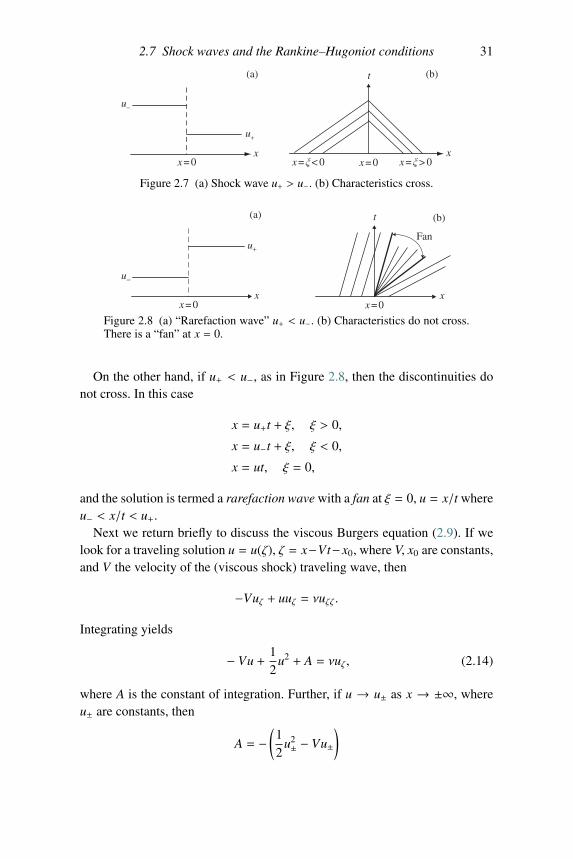
Figure 2.7 (a) Shock wave u+ > u−. (b) Characteristics cross.
Figure 2.8 (a) “Rarefaction wave” u+ < u−. (b) Characteristics do not cross.There is a “fan” at x = 0.
On the other hand, if u+ < u−, as in Figure 2.8, then the discontinuities donot cross. In this case
x = u+t + ξ, ξ > 0,
x = u−t + ξ, ξ < 0,
x = ut, ξ = 0,
and the solution is termed a rarefaction wave with a fan at ξ = 0, u = x/t whereu− < x/t < u+.
Next we return briefly to discuss the viscous Burgers equation (2.9). If welook for a traveling solution u = u(ζ), ζ = x−Vt−x0, where V, x0 are constants,and V the velocity of the (viscous shock) traveling wave, then
−Vuζ + uuζ = νuζζ .
Integrating yields
− Vu +12
u2 + A = νuζ , (2.14)
where A is the constant of integration. Further, if u → u± as x → ±∞, whereu± are constants, then
A = −(
12
u2± − Vu±
)
32 Linear and nonlinear wave equations
and by eliminating the constant A, we find
V =12
u2+ − u2−
u+ − u−=
12
(u+ + u−),
which is the same as the shock wave speed found earlier for the inviscidBurgers equation. Indeed, if we replace Burgers’ equation by the generalization
ut + (q(u))x = νuxx,
then the corresponding traveling wave u = u(ζ) would have its speed satisfy
V =q(u+) − q(u−)
u+ − u−
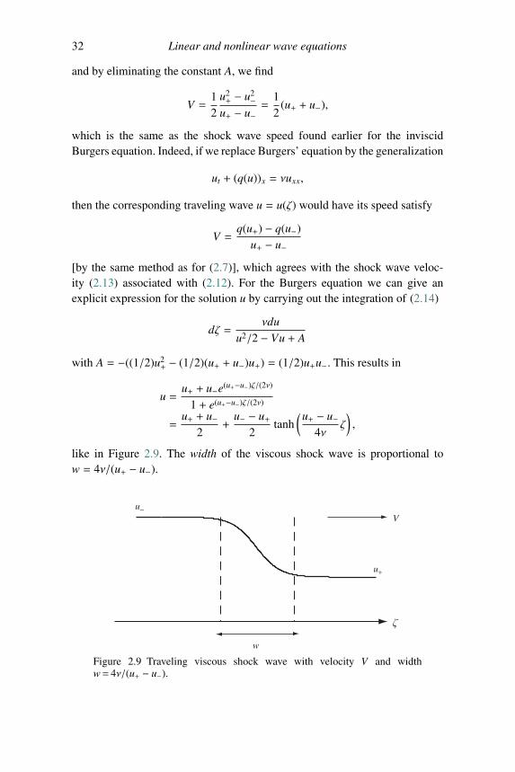
[by the same method as for (2.7)], which agrees with the shock wave veloc-ity (2.13) associated with (2.12). For the Burgers equation we can give anexplicit expression for the solution u by carrying out the integration of (2.14)
dζ =νdu
u2/2 − Vu + A
with A = −((1/2)u2+ − (1/2)(u+ + u−)u+) = (1/2)u+u−. This results in
u =u+ + u−e(u+−u−)ζ/(2ν)
1 + e(u+−u−)ζ/(2ν)
=u+ + u−
2+
u− − u+2
tanh(u+ − u−
4νζ),
like in Figure 2.9. The width of the viscous shock wave is proportional tow = 4ν/(u+ − u−).
u−
u+
w
V
Figure 2.9 Traveling viscous shock wave with velocity V and widthw= 4ν/(u+ − u−).
2.8 Second-order equations: Vibrating string equation 33
2.8 Second-order equations: Vibrating string equation
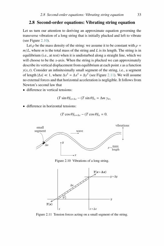
Let us turn our attention to deriving an approximate equation governing thetransverse vibration of a long string that is initially plucked and left to vibrate(see Figure 2.10).
Let ρ be the mass density of the string: we assume it to be constant with ρ =m/L, where m is the total mass of the string and L is its length. The string is inequilibrium (i.e., at rest) when it is undisturbed along a straight line, which wewill choose to be the x-axis. When the string is plucked we can approximatelydescribe its vertical displacement from equilibrium at each point x as a functiony(x, t). Consider an infinitesimally small segment of the string, i.e., a segmentof length |Δs| � 1, where Δs2 = Δx2 + Δy2 (see Figure 2.11). We will assumeno external forces and that horizontal acceleration is negligible. It follows fromNewton’s second law that• difference in vertical tensions:
(T sin θ)|x+Δx − (T sin θ)|x = Δm ytt,
• difference in horizontal tensions:
(T cos θ)|x+Δx − (T cos θ)|x = 0.
Figure 2.10 Vibrations of a long string.
Figure 2.11 Tension forces acting on a small segment of the string.
34 Linear and nonlinear wave equations
In the limit |Δx| → 0 we assume that y = y(x, t); then one has (in that limit)
sin θ =ΔyΔs=
Δy√(Δx)2 + (Δy)2
→ yx√1 + y2
x
,
cos θ =ΔxΔs→ 1√
1 + y2x
.
Hence with these assumptions, in this limit, and using dm = ρds, Newton’sequations become (
ρdsdx
)ytt − ∂
∂x
(T
yx√1 + y2
x
)= 0,
∂
∂x
(T
1√1 + y2
x
)= 0.
From the second equation we get that T = T0
√1 + y2
x , T0 constant and, usingds/dx =
√1 + y2
x, the first equation yields
ytt =T0
ρ√
1 + y2x
yxx. (2.15)
This is a nonlinear equation governing the vibrations of the string. If weconsider small-amplitude vibrations (i.e., |yx| � 1) and so neglect y2
x in thedenominator of the right-hand side we obtain, as an approximation, the linearwave equation,
ytt − c2yxx = 0,
where c2 = T0/ρ is the wave speed (speed of sound). However, we can approx-imate (2.15) by assuming that |yx| is small but without neglecting it completely.That can be done by taking the first correction term from a Taylor series of thedenominator:
1√1 + y2
x
≈ 11 + y2
x/2≈ 1 − 1
2y2
x.
Doing so leads to the nonlinear equation
ytt = c2yxx
(1 − 1
2y2
x
),
which is more amenable to analysis than (2.15), but still retains some of itsnonlinearity. It is interesting that this equation is a cubic nonlinear versionof (1.2) when ε � h2/12. Note: if yx becomes large (e.g., a “shock” is formed),then we need to go back to (2.15) and reconsider our assumptions.
2.9 Linear wave equation 35
2.9 Linear wave equation
Consider the linear wave equation
utt − c2uxx = 0,
where c = constant with the initial conditions u(x, 0) = f (x) and ut(x, 0) =g(x). Below we derive the solution of this equation given by D’Alembert.
It is helpful to change to the coordinate system
ξ = x − ct, η = x + ct.
Thus, from the chain rule we have that
∂x =12
(∂ξ + ∂η), ∂t =12c
(−∂ξ + ∂η)
and the equation transforms into[(∂ξ + ∂η)
2 − (−∂ξ + ∂η)2]u = 0.
Simplifying leads to
4uξη = 0.
The latter equation can be integrated with respect to ξ to give
uη = F(η),
where F is an arbitrary function. Integrating once more gives
u(ξ, η) = F(η) +G(ξ) = F(x + ct) +G(x − ct).
This is the general solution of the wave equation. It remains to incorporate theinitial data. We have that
u(x, 0) = F(x) +G(x) = f (x),
ut(x, 0) = cF′(x) − cG′(x) = g(x).
Differentiating the first equation leads to
f ′(x) = F′(x) +G′(x),
g(x) = cF′(x) − cG′(x).
By addition and subtraction of these equations one gets that
F′ =12
(f ′ +
gc
), G′ =
12
(f ′ − g
c
).
36 Linear and nonlinear wave equations
It follows that
F(x) =12
f (x) +12c
∫ x
0g(ζ) dζ + c1,
G(x) =12
f (x) − 12c
∫ x
0g(ζ) dζ + c2,
where c1, c2 are constants. Hence,
u(x, t) =12
[f (x + ct) + f (x − ct)
]+
12c
∫ x+ct
x−ctg(ζ) dζ + c3, c3 = c1 + c2.
Since u(x, 0) = f (x) it follows that c3 = 0 and that
u(x, t) =12
[f (x + ct) + f (x − ct)
]+
12c
∫ x+ct
x−ctg(ζ) dζ.
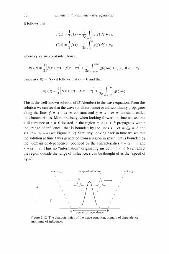
This is the well-known solution of D’Alembert to the wave equation. From thissolution we can see that the wave (or disturbance) or a discontinuity propagatesalong the lines ξ = x + ct = constant and η = x − ct = constant, calledthe characteristics. More precisely, when looking forward in time we see thata disturbance at t = 0 located in the region a < x < b propagates withinthe “range of influence” that is bounded by the lines x − ct = ξR = b andx + ct = ηL = a (see Figure 2.12). Similarly, looking back in time we see thatthe solution at time t was generated from a region in space that is bounded bythe “domain of dependence” bounded by the characteristics x − ct = a andx + ct = b. Thus no “information” originating inside a < x < b can affectthe region outside the range of influence; c can be thought of as the “speed oflight”.
Figure 2.12 The characteristics of the wave equation; domain of dependenceand range of influence.
2.10 Characteristics of second-order equations 37
2.10 Characteristics of second-order equations
We already encountered the method of characteristics in Section 2.6 for thecase of first-order equations (in the evolution variable t). The notion of charac-teristics, however, can be extended to higher-order equations, as we just saw inD’Alembert’s solution to the wave equation. Loosely speaking, characteristicsare those curves along which discontinuities can propagate. A more formal def-inition for characteristics is that they are those curves along which the Cauchyproblem does not have a unique solution. For second-order quasilinear PDEsthe Cauchy problem is given by
Auxx + Buxy +Cuyy = D, (2.16)
where we assume that A, B, C, and D are real functions of u, ux, uy, x, andy and the boundary values are given on a curve C in the (x, y)-plane in termsof u or ∂u/∂n (the latter being the normal derivative of u with respect to thecurve C).
We will not go into the formal derivation of the equations for the charac-teristics, which can be found in many PDE textbooks (see, e.g., Garabedian,1984). A quick method for deriving these equations can be accomplished bykeeping in mind the basic property of a characteristic – a curve along whichdiscontinuities can propagate, cf. Whitham (1974). One assumes that u has asmall discontinuous perturbation of the form
u = Us + εΘ(ν(x, y))Vs, (2.17)
where Us,Vs are smooth functions, ε is small, and
Θ(ν) =
{0, ν < 01, ν > 0
is the Heaviside function (sometimes denoted by H(ν)). Here ν(x, y) = constantare the characteristic curves to be found. We recall that Θ′(ν) = δ(ν), i.e.,the derivative of a Heaviside function is the Dirac delta function (cf. Lighthill1958). Roughly speaking, δ is less smooth than Θ and near ν = 0 is takento be “much larger” than Θ, which is less smooth than Us, etc. In turn, δ′ ismore singular (much larger) than δ near ν = 0, etc. When we substitute (2.17)into (2.16) we keep the highest-order terms, which are those terms that mul-tiply δ′, and neglect the less singular terms that multiply δ, Θ, and Us. Thisgives us (
Aν2x + Bνxνy +Cν2
y
)εδ′Vs + l.o.t. = 0,
38 Linear and nonlinear wave equations
(here l.o.t., lower-order terms, means terms that are less singular) or
Aν2x + Bνxνy +Cν2
y = 0. (2.18)
Since ν(x, y) = constant are the characteristics, we have that dν = νxdx+νydy =0 and therefore
dydx= −νx
νy.
Combined with (2.18), we obtain
Adydx
2
− Bdydx+C = 0 (2.19)
as the equation for the characteristic y = y(x).
2.11 Classification and well-posedness of PDEs
Based on the types of solutions to (2.19), it is possible to classify quasilinearPDEs in two independent variables. Letting λ ≡ dy/dx, we have the followingclassification (recall A, B,C are assumed real):• Hyperbolic: Two, real roots λ1 and λ2;• Parabolic: Two, real repeated roots λ1 = λ2; and• Elliptic: Two, complex conjugate roots λ1 and λ2 = λ
∗1.
The terminology comes from an analogy between the quadratic form (2.18)and the quadratic form for a plane conic section (Courant and Hilbert, 1989).
Some prototypical examples are:
(a) The wave equation: utt−c2uxx = 0 (note the interchange of variables x→ t,y→ x). Here A = 1, B = 0, C = −c2. Thus (2.19) gives(
dxdt
)2− c2 = 0,
which implies the characteristics are given by x ± ct = constant. There aretwo, real solutions. Therefore, the wave equation is hyperbolic.
(b) The heat equation: ut−uxx = 0 (in this example, y→ t). Here A = −1, B =0, C = 0. Thus (2.19) gives (
dtdx
)2= 0,
which implies the characteristics are given by t = constant. There are two,repeated real solutions. Therefore, the heat equation is parabolic.
2.11 Classification and well-posedness of PDEs 39
(c) The potential equation (often called Laplace’s equation): uxx + uyy = 0.Here A = 1, B = 0, C = 1. Thus (2.19) gives(
dydx
)2+ 1 = 0,
which implies the characteristics are given by y = ±ix + constant. Thereare two, complex solutions. Therefore, the potential equation is elliptic.
That the potential equation is elliptic suggests that we can specify “initial”data on any real curve and obtain a unique solution. However, we will see indoing this that something goes seriously wrong. This leads us to the conceptof well-posedness. To this end, consider the problem
uyy + uxx = 0,
u(x, 0) = f (x),
uy(x, 0) = g(x),
and look for solutions of the form us = exp[i(kx − ω(k)y)
]. This leads to the
dispersion relation ω = ±ik. We then have the formal solution
u(x, y) =1
2π
∫b+(k, 0) exp(ikx) exp(ky) dk
+1
2π
∫b−(k, 0) exp(ikx) exp(−ky) dk,
where b+ and b− are determined from the initial data. In general, these integralsdo not converge. To make them converge we need to require that b±(k) decaysfaster than any exponential, which generally speaking is not physically reason-able. The “problem” is that the dispersion relation growth rate, ω(k) = ±ik, isunbounded and imaginary.
Now suppose we consider the following initial data on y = 0: f (x) = 0 andg(x) = gk(x) = sin(kx)/k, where k is a positive integer. Using separation ofvariables, we find, for each value of k, the solution is
uk(x, y) =[A0 cosh(ky) + B0 sinh(ky)
]sin(kx),
where A0 and B0 are constants to be determined. Using uk(x, 0) = 0, we findthat A0 = 0. And
∂uk
∂y(x, 0) =
sin(kx)k
= B0k sin(kx)
implies B0 = 1/k2. Thus, the solution is
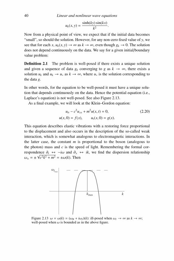
40 Linear and nonlinear wave equations
uk(x, y) =sinh(ky) sin(kx)
k2.
Now from a physical point of view, we expect that if the initial data becomes“small”, so should the solution. However, for any non-zero fixed value of y, wesee that for each x, uk(x, y)→ ∞ as k → ∞, even though gk → 0. The solutiondoes not depend continuously on the data. We say for a given initial/boundaryvalue problem:
Definition 2.1 The problem is well-posed if there exists a unique solutionand given a sequence of data gk converging to g as k → ∞, there exists asolution uk and uk → u∗ as k → ∞, where u∗ is the solution corresponding tothe data g.
In other words, for the equation to be well-posed it must have a unique solu-tion that depends continuously on the data. Hence the potential equation (i.e.,Laplace’s equation) is not well-posed. See also Figure 2.13.
As a final example, we will look at the Klein–Gordon equation:
utt − c2uxx + m2u(x, t) = 0, (2.20)
u(x, 0) = f (x), ut(x, 0) = g(x).
This equation describes elastic vibrations with a restoring force proportionalto the displacement and also occurs in the description of the so-called weakinteraction, which is somewhat analogous to electromagnetic interactions. Inthe latter case, the constant m is proportional to the boson (analogous tothe photon) mass and c is the speed of light. Remembering the formal cor-respondence ∂t ↔ −iω and ∂x ↔ ik, we find the dispersion relationshipω± = ±
√c2k2 + m2 = ±ω(k). Then
Figure 2.13 ω = ω(k) = (ωR + iωI)(k): ill-posed when ωI → ∞ as k → ∞;well-posed when ω is bounded as in the above figure.

2.11 Classification and well-posedness of PDEs 41
u(x, t) =1
2π
∫b+(k, 0) exp
⎡⎢⎢⎢⎢⎢⎣i(kx + ck
√1 +(mck
)2t
⎤⎥⎥⎥⎥⎥⎦ dk
+1
2π
∫b−(k, 0) exp
⎡⎢⎢⎢⎢⎢⎣i(kx − ck
√1 +(mck
)2t
⎤⎥⎥⎥⎥⎥⎦ dk, (2.21)
where b+ and b− will be determined from the initial data. We have
f (x) =1
2π
[∫b+(k) exp(ikx)dk +
∫b−(k) exp(ikx) dk
](2.22a)
g(x) =i
2π
[∫b+(k)ω(k) exp(ikx) dk −
∫b−(k)ω(k) exp(ikx) dk
]. (2.22b)
Let
f (k) ≡∫
f (x) exp(−ikx) dx,
g(k) ≡∫
g(x) exp(−ikx) dx;
then (2.22) implies that
f = b+ + b−,−igω= b+ − b−.
Solving this system and substituting back into (2.21), we find that
u(x, t) =1
4π
∫ (f (k) − ig(k)
ω(k)
)exp [i(kx + ω(k)t] dk
+1
4π
∫ (f (k) +
ig(k)ω(k)
)exp [i(kx − ω(k)t] dk.
As an example, for the specific initial data u(x, 0) = δ(x), where δ(x) is theDirac delta function, we have ut(x, 0) = 0, and so f (k) = 1 and g(k) = 0. Thus,
u(x, t) =1
2π
∫eikx cos [ω(k)t] dk,
which due to sin(kx) being an odd function simplifies to
u(x, t) =1
2π
∫cos(kx) cos [ω(k)t] dk.
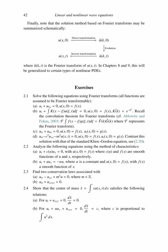
42 Linear and nonlinear wave equations
Finally, note that the solution method based on Fourier transforms may besummarized schematically:
u(x, 0)Direct transformation−−−−−−−−−−−−−−−→ u(k, 0)⏐⏐⏐⏐⏐*Evolution
u(x, t)Inverse transformation←−−−−−−−−−−−−−−− u(k, t)
.
where u(k, t) is the Fourier transform of u(x, t). In Chapters 8 and 9, this willbe generalized to certain types of nonlinear PDEs.
Exercises
2.1 Solve the following equations using Fourier transforms (all functions areassumed to be Fourier transformable):(a) ut + u5x = 0, u(x, 0) = f (x).(b) ut +
∫K(x − ξ)u(ξ, t)dξ = 0, u(x, 0) = f (x), ˆK(k) = e−k2
. Recallthe convolution theorem for Fourier transforms (cf. Ablowitz andFokas, 2003: F ∫ f (x − ξ)g(ξ, t)dξ = F(k)G(k) where F representsthe Fourier transform).
(c) utt + u4x = 0, u(x, 0) = f (x), ut(x, 0) = g(x).(d) utt−c2uxx−m2u(x, t) = 0, u(x, 0) = f (x), ut(x, 0) = g(x). Contrast this
solution with that of the standard Klien–Gordon equation, see (2.20).2.2 Analyze the following equations using the method of characteristics:
(a) ut + c(u)ux = 0, with u(x, 0) = f (x) where c(u) and f (x) are smoothfunctions of u and x, respectively.
(b) ut + uux = −αu, where α is a constant and u(x, 0) = f (x), with f (x)a smooth function of x.
2.3 Find two conservation laws associated with(a) utt − uxx + m2u = 0, where m ∈ R.(b) utt + uxxxx = 0.
2.4 Show that the center of mass x =∫
xu(x, t) dx satisfies the following
relations:
(a) For ut + uxxx = 0,dxdt= 0.
(b) For ut + uux + uxxx = 0,dxdt= c, where c is proportional to∫
u2 dx.
Exercises 43
2.5 Use D’Alembert’s solution to solve the initial value problem of the waveequation on the semi-infinite line
utt − c2uxx = 0,
c constant, where u(x, 0) = f (x), ut(x, 0) = g(x), x > 0 and either(a) u(0, t) = h(t) or(b) ut(0, t) = h(t).
2.6 Consider the PDE
utt − uxx + σuxxxx = 0,
whereσ = ±1. Determine for which values ofσ that the equation is well-posed and solve the Cauchy problem for the case where the equation iswell-posed.
2.7 Consider the equation
ut + uux = 0,
with initial condition u(0, x) = cos(πx).(a) Find the (implicit) solution of the equation.(b) Show that u(x, t) has a point t = tB where ux is infinite. Find tB.(c) Describe the solution beyond t = 1/π.
2.8 (a) Solve the Cauchy problem
ux + uuy = 1, u(0, y) = ay,
where a is a non-zero constant.(b) Find the solution of the equation in part (a) with the data
x = 2t, y = t2, u(0, t2) = t.
Hint: The following forms are equivalent:
dx1=
dyu=
du1
anddxds= 1,
dyds= u,
duds= 1.
2.9 Consider the equation
ut + uux = 1, −∞ < x < ∞, t > 0.
(a) Find the general solution.(b) Discuss the solution corresponding to: u = 1
2 t when t2 = 4x.(c) Discuss the solution corresponding to: u = t when t2 = 2x.
44 Linear and nonlinear wave equations
2.10 Solve the equation
ut + uux = 0, −∞ < x < ∞, t > 0,
subject to the initial data
u(x, 0) =
⎧⎪⎪⎪⎪⎪⎨⎪⎪⎪⎪⎪⎩0, x ≤ 0
x/a, 0 < x < a
1, x ≥ a.
Examine the solution as a→ 0.2.11 Find the the solution of the equation
yux − xuy = 0,
corresponding to the data u(x, 0)= f (x). Explain what happens if we giveu(x(s), y(s))= f (s) along the curve defined by {s : x2(s) + y2(s)= a2}.
2.12 Find the solution to the initial value problem
ut + u3ux = 0,
u(x, 0) = f (x).
Find the solution when f (x) = x1/3 and discuss its behavior as t → ∞.2.13 Use the traveling wave coordinate ξ = x − ct to reduce the PDE
ut − uxx =
{u, 0 ≤ u ≤ 1/20, 1/2 ≤ u ≤ 1.
to an ODE. Solve the ODE subject to the boundary conditions u(−∞) = 1and u(+∞) = 0. Discuss the solution for c = 2 and c � 2.
3Asymptotic analysis of wave equations: Properties and
analysis of Fourier-type integrals
In the previous chapter we constructed the solution of equations using Fouriertransforms. This yields integrals that depend on parameters describing spaceand time variation. When used with asymptotic analysis the Fourier methodbecomes extremely powerful. Long-time asymptotic evaluation of integralsyields the notion of group velocity and the structure of the solution. In thischapter, we apply these techniques to the linear Schrodinger equation, the lin-ear KdV equation, discrete equations, and to the Burgers equation, which isreduced to the heat equation via the Hopf–Cole transformation.
Consider the asymptotic behavior of Fourier integrals resulting from the useof Fourier transforms (see Chapter 2). These integrals take the form
u(x, t) =1
2π
∫u(k) exp [i(kx − ω(k)t)] dk (3.1)
in the limit as t → ∞ with χ ≡ x/t held fixed, i.e., we will study approxima-tions to (3.1) for large times and for large distances from the origin. We canrewrite this integral in a slightly more general form by defining φ(k) ≡ kχ − ω(for simplicity of notation here we suppress the dependence on χ in φ) andconsidering integrals of the form
I(t) =∫ b
au(k) exp
[iφ(k)t
]dk, (3.2)
where we assume φ(k) is smooth on −∞ ≤ a < b ≤ ∞. First, by the Riemann–Lebesgue lemma (cf. Ablowitz and Fokas, 2003), provided u(k) ∈ L1(a, b), wehave
limt→∞ I(t) = 0.
But this does not provide any additional qualitative information. Insight canbe obtained if we assume that both u(k) and φ(k) are sufficiently smooth. Ifφ′(k) � 0 in [a, b], then we can rewrite (3.2) as
45
46 Asymptotic analysis of wave equations∫ b
a
u(k)iφ′(k)t
ddk
eiφ(k)tdk;
then integrating by parts gives
I(t) = eiφ(k)t u(k)iφ′(k)t
∣∣∣∣∣∣ba
−∫ b
aexp[iφ(k)t
] ddk
(u(k)
iφ′(k)t
)dk.
Repeating the process we can show that the second term is of order 1/t2.1 Thus,we have
I(t) = i
[u(a)eiφ(a)t
φ′(a)− u(b)eiφ(b)t
φ′(b)
]1t+ O(1/t2).
If u(k) and φ′(k) are C∞ (i.e., infinitely differentiable) functions, then we maycontinue to integrate by parts to get the asymptotic expansion
I(t) ∼∞∑
n=1
cn(t)tn
,
where the cn are bounded functions. Notice that if u ∈ L1(−∞,∞), then
lima→−∞ u(a) = lim
b→∞u(b) = 0.
Therefore, if φ′(k) � 0 for all k and if both u(k), φ(k) ∈ C∞, then we have
u(x, t) = o(t−n), n = 1, 2, 3, . . . , (3.3)
i.e., u goes to zero faster than any power of t.It is more common, however, that there exists a point or points where
φ′(c) = 0. The technique used to analyze this case is called the method ofstationary phase, which was originally developed by Kelvin (cf. Jeffreys andJeffreys, 1956; Ablowitz and Fokas, 2003). We will explore this technique now.
3.1 Method of stationary phase
When considering the Fourier integral (3.2), we wish to determine the long-time asymptotic behavior of I(t). As our previous analysis shows, intuitively,for large values of t, there is very rapid oscillation, leading to cancellation. But,the oscillation is less rapid near points where φ′(k) = 0 and the cancellationwill not be as complete. We will call a point, k, where φ′(k) = 0, a stationarypoint.
1 We say that u = O(t−n) if limt→∞ |u|tn = constant and u = o(t−n) if limt→∞ |u|tn = 0. See alsoSection 3.2 for the definitions of big “O”, little “o” and asymptotic expansions.
3.1 Method of stationary phase 47
Suppose there is a so-called stationary point c, a < c < b, such that φ′(c) = 0,φ′′(c) � 0 and u(c) exists and is non-zero. In addition, suppose u(k) and φ(k)are sufficiently smooth. Then we expect that the dominant contribution to (3.2)should come from a neighborhood of c, i.e., the leading asymptotic term is
I(t) ∼∫ c+ε
c−εu(c) exp
[i
(φ(c) +
φ′′(c)2
(k − c)2
)t
]dk, (3.4)
= u(c) exp(iφ(c)t)∫ c+ε
c−εexp
[iφ′′(c)
2(k − c)2t
]dk,
where ε is small. Let
ξ2 =|φ′′(c)|
2(k − c)2t, μ ≡ sgn(φ′′(c)).
Then (3.4) becomes
I(t) ∼√
2t|φ′′(c)| u(c) exp(iφ(c)t)
∫ ε
√t|φ′′(c)|
2
−ε√
t|φ′′(c)|2
exp(iμξ2) dξ.
For |φ′′(c)| = O(1), extending the limits of integration from −∞ to ∞, i.e., wetake ε
√t → ∞, yields the dominant term. The integral∫ ∞
−∞exp(iμξ2) dξ =
√π exp
(iμπ
4
),
is well known, hence
I(t) ∼ u(c)
√2π
t|φ′′(c)| exp(iφ(c)t + iμ
π
4
). (3.5)
If we are considering Fourier transforms, we have φ(k) = kχ − ω(k), forwhich φ′(k) = 0 implies
χ =xt= ω′(k0) (3.6)
for a stationary point k0. Or, assuming ω′ has an inverse, k0 = (ω′)−1(x/t) ≡k0(x/t). In addition, if we are working with a dispersive PDE, then bydefinition, except at special points, φ′′(k) � 0. Substituting this into (3.5),
u(x, t) ∼ u(k0)√2πt|φ′′(k0)| exp
(iφ(k0)t + iμ
π
4
), (3.7)
which can be rewritten as
u(x, t) ∼ A(x/t)√t
exp (iφ(k0)t) , (3.8)
48 Asymptotic analysis of wave equations
where A(x/t)/√
t is the decaying in time, slowly varying, complex amplitude.This decay rate, O(1/
√t), is slow, especially when compared to those cases
when the solution decays exponentially or as O(1/tn) for n large. Note thatdimensionally, ω′ corresponds to a speed. Stationary phase has shown that theleading-order contribution comes from a region moving with speed ω′, whichis termed the group velocity. This is the velocity of a slowly varying packet ofwaves. We will see later that this is also the speed at which energy propagates.
Example 3.1 Linear KdV equation: ut + uxxx = 0. The dispersion relation isω = −k3 and so φ(k) = kx/t + k3. Thus, the stationary points, satisfying (3.6),occur at k0 = ±√−x/(3t) so long as x/t < 0. Note that we might expectsomething interesting to happen as x/t → 0, since φ′(k) vanishes there andimplies a higher-order stationary point. We also expect different behavior whenx/t > 0 since k0 becomes imaginary there.
Example 3.2 Free-particle Schrodinger equation: iψt + ψxx = 0, |x| < ∞,ψ(x, 0) = f (x), and ψ→ 0 as |x| → ∞. This is a fundamental equation in quan-tum mechanics. The wavefunction, ψ, has the interpretation that |ψ(x, t)|2dx isthe probability of finding a particle in dx, a small region about x at time t.The dispersion relation ω = k2 shows that the stationary point satisfying (3.6)occurs at k0 = x/(2t).
3.2 Linear free Schrodinger equation
Now we will consider a specific example of the method of stationary phase asapplied to the linear free Schrodinger equation
iut + uxx = 0. (3.9)
First assume a wave solution of the form us = ei(kx−ω(k)t), substitute it into theequation and derive the dispersion relation
ω(k) = k2.
Notice that ω is real and ω′′(k) = 2 � 0 and hence solutions to (3.9) are in thedispersive wave regime. Thus the solution, via Fourier transforms, is
u(x, t) =1
2π
∫u0(k)ei(kx−k2t) dk,
where u0(k) is the Fourier transform of the initial condition u(x, 0) = u0(x). Asbefore, to apply the method of stationary phase, we rewrite the exponential inthe Fourier integral the following way
3.2 Linear free Schrodinger equation 49
u(x, t) =1
2π
∫u0(k)eiφ(k)t dk,
where φ(k) = kχ − k2 with χ = x/t. The dominant contribution to the integraloccurs at a stationary point k0 when φ′(k0) = 0; k0 = x/(2t) in this case. Notingthat sgn(φ′′(k0)) = −1, the asymptotic estimate for u(x, t) using (3.7) is
u(x, t) =u0
(x2t
)√
4πtexp
(i( x2t
)2t − i
π
4
)+ o
(1√
t
). (3.10)
A more detailed analysis, using the higher-order terms arising from the Taylorseries of u(k) and φ(k) near k = k0, shows that if u0(k) ∈ C∞ then we have themore general result
u(x, t) ∼ 1√4πt
exp
(i( x2t
)2t − i
π
4
) ⎡⎢⎢⎢⎢⎢⎣u0( x2t ) +
∞∑n=1
gn( x2t )
(4it)n
⎤⎥⎥⎥⎥⎥⎦ ,where gn(y) are related to the higher derivatives of u0 (see Ablowitz and Segur,1981).
Definition 3.3 The function I(t) has an asymptotic expansion around t = t0(Ablowitz and Fokas, 2003) in terms of an ordered asymptotic sequence{δ j(t)} if(a) δ j+1(t) � δ j(t), as t → t0, j = 1, 2, . . . , n, and(b) I(t) =
∑nj=1 a jδ j(t) + Rn(t) where the remainder Rn(t) = o(δn(t)) or
limt→t0
∣∣∣∣∣Rn(t)δn(t)
∣∣∣∣∣ = 0.
The notation δ j+1(t) � δ j(t), means
limt→t0
∣∣∣∣∣∣δ j+1(t)
δ j(t)
∣∣∣∣∣∣ = 0.
We also write
I(t) ∼n∑
j=1
a jδ j(t),
which says I(t) has the asymptotic expansion given on the right-hand side ofthe symbol “∼”. Notice that if n = ∞, then we mean Rn(t) = o(δn(t)) for all n.Asymptotic series expansions may not (usually do not) converge.
The asymptotic solution (3.10) can be viewed as a “slowly varying” sim-ilarity or self-similar solution. In general, a similarity solution takes theform
50 Asymptotic analysis of wave equations
u(x, t) =1tp
f( xtq
), (3.11)
for suitable constants p and q. This important concept describes phenomenain terms of a reduced number of variables, when time and space are suitablyrescaled. Similarity solutions find important applications in many areas of sci-ence. One well-known example is that of G.I. Taylor who in the 1940s founda self-similar solution to the problem of determining the shock-wave radiusand speed after an (nuclear) explosion (Taylor, 1950). He found that the frontof an approximately spherical blast wave is described self-similarly with theindependent variables scaled according to a two-fifths law, r/t2/5, where r isthe radial distance from the origin.
We determine the similarity solution to the linear Schrodinger equation byassuming the form (3.11) and inserting it into (3.9); i.e., we assume the ansatz
usim(x, t) =1tp
f (η) where η =xtq
. Then we find the relation
f ′′
tp+2q− i
(p f
tp+1+
qη f ′
tp+1
)= 0.
In order to keep all the powers of t the same, we require 2q = 1 but p canbe arbitrary. In general, linear equations do not determine both p and q butnonlinear equations usually fix both. For linear equations, p is fixed by addi-tional information; e.g., initial values or side conditions. For the linear freeSchrodinger equation we take p = 1/2, motivated by our previous analysiswith the stationary phase technique. Then our equation takes the form
f ′′ − i2
(η f ′ + f ) = 0,
which we can integrate directly to obtain
f ′ − i2η f = c1, c1 const.
Introducing the integrating factor e−iη2/4, we integrate this equation to find
f (η) = c1
∫ei(η2−(η′)2)/4dη′ + c2eiη2/4, c2 const.
If c1 = 0, we have the similarity solution
usim(x, t) =c2√
texp
(i4
( xt
)2t
)=
c2√4πt
exp(iη2 − iπ/4
),
where η =x
2√
t, c2 =
c2√4π
e−iπ/4.
3.3 Group velocity 51
By identifying the “constant of integration” c2, with the slowly varying func-tion u0(x/t), we can write the asymptotic solution, obtained earlier via themethod of stationary phase, (3.10), as
u(x, t) ∼ u0(x/(2t))usim(x, t) =u0(x/(2t))√
4πtei(x/(2t))2te−iπ/4. (3.12)
In the argument of the first term u0, the spatial coordinate, x, is scaled by 1/2tbut in the second term (eix2/(4t) = ei(x/(2
√t))2
), x is scaled by 1/√
t. For largevalues of t, the first term varies in x much more slowly than the second term.We refer to this as a slowly varying similarity solution. In a sense usim(x, t)is an “attractor” for this linear problem. Slowly varying similarity solutionsarise frequently – even for certain nonlinear problems such as the nonlinearSchrodinger equation
iut + uxx ± |u|2u = 0,
e.g., see Ablowitz and Segur (1981).
3.3 Group velocity
Recall that the “group velocity”, defined to be ω′(k), enters into the method ofstationary phase through the solution of the equation φ′(k) = 0; i.e., through thestationary points. We have seen that, for linear problems, the dominant termsin the solution come from the region near the stationary points. The energy canbe shown to be transported by the group velocity. Next we describe this usinga different asymptotic procedure.
Frequently we look directly for slowly varying wave groups in order toapproximate the solution; see Whitham (1974). Suppose we consider, basedon our stationary phase result, that the solution to a linear dispersive waveproblem [e.g., the linear Schrodinger equation (3.9)] is of the form
u(x, t) ∼ A(x, t)eiθ(x,t), t � 1, (3.13)
A(x, t) =1√
tg(x/t),
θ(x, t) = (k0(x/t)x/t − ω(k0(x/t)))t = φ(x/t)t,
where g and φ are slowly varying. That is,
∂g∂x=
1t
g′(
xt
)� 1 and
∂g∂t= − x
t2g′(
xt
)� 1;
52 Asymptotic analysis of wave equations
also∂φ
∂x� 1 and
∂φ
∂t� 1. Notice that θ is rapidly varying. To generalize the
notion of wavenumber and frequency as defined in Section 2.2, we take
∂θ
∂x= φ′(x/t) = k0 (3.14)
∂θ
∂t= φ(x/t) − (x/t)φ′(x/t) = k0x/t − ω(k0) − k0x/t = −ω(k0), (3.15)
where we used (3.13). So we can define the slowly varying wavenumber andfrequency by the above relations. The ansatz (3.13) with a rapidly varyingphase (or the real part in cases where the solution u is real) for wave-like prob-lems is sometimes called the WKB approximation (after Wentzel–Kramer–Brillouin) for wave problems. Many linear problems we see naturally havesolutions of the WKB type. In fact there exists a wide range of nonlinearproblems that admit generalizations of such rapidly varying phase solutions.In Chapter 4 we will study ODEs where such rapidly varying phase methods(i.e., WKB methods) are useful.
From relations (3.14) and (3.15), we find that (dropping the subscript on k)
kt =∂2θ
∂t∂x=
∂2θ
∂x∂t= −ωx (3.16a)
kt + ωx = 0 (3.16b)
kt + ω′(k)kx = 0. (3.16c)
Equation (3.16b), which follows from (3.16a), is the so-called conservation ofwave equation. Assumingω = ω(k), equation (3.16c) is a first-order hyperbolicPDE that, as we have seen, can be solved via the method of characteristics. Itfollows (see Chapter 2) that k(x, t) is constant along group lines (curves) inthe (x, t)-plane defined by dx/dt = ω′(k(x, t)) for any slowly varying wavepacket.
Now we will show that the energy in the asymptotic solution to (3.13) prop-agates with the group velocity. Recall that the energy in the solution of a PDEis proportional to the L2-norm in space. We will limit ourselves to the interval[x1(t), x2(t)] as the region of integration to find the energy in a wave packet.For this approximation, we have
Q(t) =∫ x2(t)
x1(t)|A|2 dx.
3.3 Group velocity 53
Differentiating this quantity with respect to t we find
dQdt=
∫ x2(t)
x1(t)
∂
∂t|A|2 dx + |A|2(x2)
dx2
dt− |A|2(x1)
dx1
dt
=
∫ x2(t)
x1(t)
{∂
∂t|A|2 + ∂
∂x(|A|2ω′(k))
}dx, (3.17)
where we used the characteristic curvesdx2
dt= ω′(k2) and
dx1
dt= ω′(k1) with
k remaining constant along them.Notice in our notation that A = g(x/t)/
√t is associated with the long-time
asymptotic result (3.7)–(3.8). So let us substitute this into the expression forQ(t) to get
Q(t) =∫ x2(t)
x1(t)
1t
∣∣∣∣g ( xt
)∣∣∣∣2 dx.
Now make the change of variable u = x/t and, along with the relations from
the characteristic curves,dx2
dt= ω′(k2) and
dx1
dt= ω′(k1), we have
Q(t) =∫ ω′(k2)+c2/t
ω′(k1)+c1/t|g(u)|2du,
where c1, c2 are constants, and that for t � 1 is asymptotically constant intime. Thus to leading order the quantity Q(t) is conserved, i.e., dQ/dt = 0.Thus returning to (3.17), since x1, x2 are arbitrary, we find the conservationequation
∂
∂t|A|2 + ∂
∂x(ω′(k)|A|2) = 0. (3.18)
The energy density, |A|2, shows that the group velocity ω′(k), associated withthe energy flux term ω′(k)|A|2, is the velocity with which the energy is trans-ported. We also note that this equation is of the same form as the conservationof mass equation from fluid dynamics
∂ρ
∂t+∂
∂x(uρ) = 0,
which is discussed later in this book. Here, ρ is the fluid density and u is thevelocity of the fluid.
Another way to derive (3.18) is directly from the PDE itself. For the linearfree Schrodinger equation, using
u∗(iut + uxx) = 0,
u(−iu∗t + u∗xx
)= 0,
54 Asymptotic analysis of wave equations
where u∗ is the complex conjugate, and then subtracting these two equations,we find
i(utu∗ + uu∗t
)+ u∗uxx − uu∗xx = 0,
i∂
∂t|u|2 + ∂
∂x(u∗ux − uu∗x
)= 0,
∂
∂tT +
∂
∂xF = 0,
which we have seen is a conservation law with density T and flux F. Assumingu = Aeiθ, we have T = |A|2, as the conserved energy, and the term F is
F = −i(u∗ux − uu∗x
),
= −i(A∗e−iθ(iAθx + Ax)eiθ − Aeiθ (−iA∗θx + A∗x
)e−iθ).
Recall that A is slowly varying so |Ax| =∣∣∣A∗x∣∣∣ � 1; dropping these terms and
substituting the generalized wavenumber relation (3.14), θx ∼ k and ω′ ∼ 2k,the flux turns out to be, at leading order for t � 1,
F = 2k|A|2 = ω′(k)|A|2.Thus we have again found (3.18) for large time.
3.4 Linear KdV equation
The linear Korteweg–de Vries (KdV) equation (which models the unidirec-tional propagation of small-amplitude long water waves or shallow-waterwaves) is given by
ut + uxxx = 0. (3.19)
In this section we will use multiple levels of asymptotics, the method ofstationary phase as discussed before, the method of steepest descent, andself-similarity, to find the long-time behavior of the solution. There are threeasymptotic regions to consider:• x/t < 0;• x/t > 0;• x/t → 0.The asymptotic solutions found in each of these regions will be “connected”via the Airy function, which is the relevant self-similar solution for thisproblem.
3.4 Linear KdV equation 55
The Fourier solution to (3.19) is given by
u(x, t) =1
2π
∫u0(k)ei(kx−ω(k)t) dk.
Substituting this into (3.19), the dispersion relation is found to be ω(k) = −k3,which implies
u(x, t) =1
2π
∫u0(k)ei(kx+k3t) dk.
By the convolution theorem, see Ablowitz and Fokas (2003) this can also bewritten in the form
u(x, t) =1
(3t)1/3
∫Ai
(x − x′
(3t)1/3
)u0(x′) dx′,
where Ai denotes the the Airy function; see (3.22)–(3.23).
3.4.1 Stationary phase, x/t < 0
The method of stationary phase uses the Fourier integral in the form
u(x, t) =1
2π
∫u0(k)eiφ(k)t dk,
where φ = kχ + k3 and χ = x/t. The important quantities are φ′ = χ + 3k2 = 0,
k0± = ±√−x
3t, and φ′′ = 6k. Stationary phase is applied only for real stationary
points. In this case, when x/t < 0, k0± = ±√|x/(3t)| are real.
Since we have two stationary points, we add the contributions from both ofthem to form our asymptotic estimate. Recalling that the general form of thestationary phase result is
u(x, t) ∼∑
j
u0(k0 j)√2πt|φ′′(k0 j)|
eiφ(k0 j)t+iμ jπ/4,
where the sum is over all stationary points, we have, in our particular case,
φ(k0±) = ∓2∣∣∣∣∣ x3t
∣∣∣∣∣3/2 ,φ′′(k0±) = ±2
√3
√∣∣∣∣∣ xt∣∣∣∣∣,
μ± = sgn(φ′′(k0±)) = ±1,
u(x, t) ∼
∣∣∣∣∣u0
(√∣∣∣ x3t
∣∣∣)∣∣∣∣∣√πt∣∣∣ 3x
t
∣∣∣1/4 cos[2∣∣∣ x
3t
∣∣∣3/2 t − π4 − ψ0
(√∣∣∣ x3t
∣∣∣)] , (3.20)
56 Asymptotic analysis of wave equations
where we define u0(k) ≡ |u0(k)|eiψ0(k) and use the relation u0(k) = u∗0(−k).Equation (3.20) is the leading asymptotic estimate for t � 1, when x/t < 0.
3.4.2 Steepest descent, x/t > 0
In this section we introduce the asymptotic method of steepest descent byworking through an example with the linear KdV equation (3.19). The steep-est descent technique is similar to that of stationary phase except we define ourFourier integral with complex-valued φ as follows
I(t) =∫
Cf (z)etφ(z) dz,
where C is, in general, a specified contour, which for Fourier integrals is(−∞,∞). In contrast, the stationary phase method uses the exponential in theform eiφ(k)t where φ(k) ∈ R and the contour C is the interval (−∞,∞). We areinterested in the long-time asymptotic behavior, t � 1. We can find the dom-inant contribution to I(t) whenever we can deform (by Cauchy’s theorem ifdeformations are allowed) on to a new contour C′ called the steepest descentcontour, defined to be the contour where φ(z) has a constant imaginary part:Im φ(χ) = constant. The theory of complex variables then shows that Re{φ}has its most rapid change along the steepest descent path (Ablowitz and Fokas,2003; Erdelyi, 1956; Copson, 1965; Bleistein and Handelsman, 1986). Hence,this asymptotic scheme will incorporate contributions from points along thesteepest descent contour with the most rapid change, namely at saddle points,φ′(z0) = 0 corresponding to a local maxima. The method takes the followinggeneral steps:(a) Find the saddle points φ′(z0) = 0; they can be complex.(b) Use Cauchy’s theorem to deform the contour C to C′, the steepest descent
contour through a saddle point z0. The steepest descent contour is definedby Im{φ(z)} = Im{φ(z0)}. Use Taylor series to expand about the sad-dle point and keep only the low-order terms when finding the dominantcontribution.
Let us now study the asymptotic solution for the KdV equation (3.19) withx/t > 0. The Fourier solution takes the form
u(x, t) =1
2π
∫C
u0(k)etφ(k) dk
where φ(k)= i(k x / t + k3) and C is the real axis: −∞< k<∞. In this regime,x/t > 0, φ′(k) � 0 for all k ∈ C, and we can perform integration by parts,as in (3.3), to prove that u(x, t) ∼ o(t−n) for all n. But this does not give usthe exact rate of decay, though we expect it is exponential. Steepest descent
3.4 Linear KdV equation 57
gives the exponential rate of decay under suitable assumptions. First we findthe saddle points: φ′(k) = i(x/t + 3k2) = 0 implies that we have two saddle
points, k± = ±i√
x3t .
Next, we determine the steepest descent contour: we wish to find the curvesdefined by the relations Im{φ(k) − φ(k±)} = 0 and choose one that “makessense”, namely that the integral will converge along our choice of contour. Inpractice, one can expand φ(k) in a Taylor series near a saddle point, keep thesecond-order terms, and use them to determine the steepest descent contour. Inour case, this gives
Im{φ(k) − φ(k±)} = Im
{φ′′(k±)
2(k − k±)2
}= Im
{∓3(
x3t
)1/2r2±e2iθ±
}= 0
where we have defined k − k± = r±eiθ± .
Let us first look at the case k+: We wish to make Im{−3(
x3t
)1/2r2e2iθ
}= 0
for all x/t > 0. This requires that Im{e2iθ} = 0 or sin(2θ) = 0. This is true whenθ = 0, π/2, π, 3π/2, 2π, . . . In order to choose a specific contour, we mustget a convergent result when integrating along this contour. In particular, weneed Re
{−3(x/3t)1/2r2e2iθ
}< 0 or − cos(2θ) < 0 so that we have a decaying
exponential. Therefore, we choose θ = 0, π.Now, for the k− case, the choices for θ are the same as before, namely
Im{φ(k) − φ(k−)} = 0 when θ = 0, π/2, π, 3π/2, 2π, . . . But this time, theconvergent integral relation for the real part requires that cos(2θ) < 0, so θ
must be π/2 or 3π/2. We can rule out these choices by considering the contour
that passes through the point k− = −i√
x3t . Starting at −∞, it is impossible to
pass through the point k− with local angle π/2 or 3π/2 and continue on to +∞.There is a “turn” at k− that sends the contour down to −i∞ and we cannot reach+∞ as required.
Our contour locally (near k+) follows the curve C′ ={reiθ ∈ C
∣∣∣∣∣ reiθ =
k − i√
x3t , k ∈ (−∞,∞)
}. Of the two possible choices for θ, we take θ= 0 so
that we have a positively oriented contour. In order to satisfy Cauchy’s theo-rem, we must smoothly transition from −∞ up to the curve defined near k+ andthen back down to +∞. This is not a problem for us as we are only interestedin what happens on the contour near k+.
Now that we have found our steepest descent contour, we evaluate theFourier integral along this contour using Cauchy’s theorem. Assuming no polesbetween the contours C and C′, we deform the contour C to C′ and find the
58 Asymptotic analysis of wave equations
asymptotic estimate, with the dominant contribution from the saddle point k+,to be
u(x, t) ∼ 12π
∫C′
u0(k+)etφ(k+)et2 φ′′(k+)(z−k+)2
dz,
=1
2πu0
(i√
x3t
)e−2
( x3t
)3/2t∫ ∞
−∞e−3
√x3t r2t dr,
=
u0
(i√
x3t
)2π√
t(
3xt
)1/4 e−2( x
3t
)3/2t∫ ∞
−∞e−s2
ds,
=
u0
(i√
x3t
)2√πt(
3xt
)1/4 e−2( x
3t
)3/2t. (3.21)
In going from the first line to the second line, we made the change of variable
z− k+ = r. From the second line to the third, the substitution r = s/√
3t(
x3t
)1/2was made. The last line results from the evaluation of the Gaussian integral∫
e−s2ds =
√π. We also assumed that u0(k) is analytically extendable in the
upper half-plane. If u0(k) had poles between C and C′, then these contribu-tions would need to be included; indeed they would be larger than the steepestdescent contribution.
3.4.3 Similarity solution, x/t → 0
Motivated by the formulas (3.20) and (3.21), let us look for a similarity solutionof the linear KdV equation (3.19) with the form
usim(x, t) =1
(3t)pf(
x(3t)q
).
Substituting this ansatz into (3.19) and calling η = x/(3t)q, we obtain theequation
f ′′′
(3t)p+3q− 1
(3t)p+1(3p f + 3qη f ′) = 0.
To obtain an ODE independent of t requires q = 1/3; for a linear problem; p isfree and is fixed depending on additional (e.g., initial) conditions. The aboveasymptotic analysis to the IVP implies (based on asymptotic matching of thesolution – see below) that p = 1/3 as well. Integrating the above equation oncegives
f ′′ − η f = c1 = 0, (3.22)
3.4 Linear KdV equation 59
where we take f → 0 as η → ∞. This equation is known as Airy’s equation.The bounded solution to this ODE is a well-known special function of mathe-matical physics and is denoted by Ai(η) (up to a multiplicative constant), whichhas the integral representation (Ablowitz and Fokas, 2003)
Ai(η) =1
2π
∫ ∞
−∞ei(sη+s3/3) ds. (3.23)
As with the linear Schrodinger equation (3.12), we can now write the self-similar asymptotic solution to the linear KdV equation as
u(x, t) ∼ u0(0)usim(x, t) =u0(0)(3t)1/3
Ai(
x(3t)1/3
).
An alternative, and in this case improved, way of doing this is starting with theFourier integral solution of this equation (as we have done before)
u(x, t) =1
2π
∫u0(k)ei(kx+k3t) dk
and changing the integration variable to s defined by k = s/(3t)1/3. This gives
u(x, t) =1
2π(3t)1/3
∫u0
( s
(3t)1/3
)exp
{i
(sx
(3t)1/3+
s3
3
)}ds.
Note that when x/(3t)1/3 = O(1) (recall x/t is small) the exponent is not rapidlyvarying. We assume u(k) is smooth. Therefore, as t → ∞ we can expand u0
inside the integral in a Taylor series, which gives
u(x, t) =u0(0)
2π(3t)1/3
∫ei(sη+s3/3) ds +
u′0(0)
2π(3t)2/3
∫sei(sη+s3/3) ds + · · · ,
where η = x/(3t)1/3. Using
Ai′(η) =1
2π
∫ ∞
−∞isei(sη+s3/3)ds,
we arrive at the asymptotic expansion for x/(3t)1/3 = O(1),
u(x, t) ∼ u0(0) Ai(η)(3t)1/3
− iu′0(0)Ai′(η)
(3t)2/3+ · · · . (3.24)
3.4.4 Matched asymptotic expansion
We have succeeded in determining the asymptotic behavior of the solution tothe linear KdV equation (3.19) in three different regions: x/t < 0, x/t →0, and x/t > 0. Each region required a different asymptotic technique. Now
60 Asymptotic analysis of wave equations
we will see how the Airy function matches the seemingly disparate solutionstogether.
Either applying the method of steepest descent directly on the integral solu-tion (3.23) of the Airy equation (Ablowitz and Fokas, 2003) or consulting areference such as the Handbook of Mathematical Functions (Abramowitz andStegun, 1972) reveals that
Ai(η) ∼ e−23 η
3/2
2√πη1/4
as η→ +∞,
Ai(η) ∼cos(
23η
3/2 − π/4)
√π|η|1/4 as η→ −∞.
Then we rewrite (3.20) and (3.21) in the following form:
u(x, t) ∼
∣∣∣∣∣u0
(i(
x3t
)1/2)∣∣∣∣∣2√π
e− 2
3
(x
(3t)1/3
)3/2(3t)1/3
(x
(3t)1/3
)1/4 , xt> 0
u(x, t) ∼
∣∣∣∣∣u0
(∣∣∣ x3t
∣∣∣1/2)∣∣∣∣∣√π
cos(
23
∣∣∣∣ x(3t)1/3
∣∣∣∣3/2 − π4 − ψ0
(∣∣∣ x3t
∣∣∣1/2))(3t)1/3
∣∣∣∣ x(3t)1/3
∣∣∣∣1/4 ,xt< 0.
Comparing the previous two sets of equations, we will see that this can beinterpreted as a slowly varying similarity solution involving the Airy functionthat matches the asymptotic behavior in all three regions. Calling η = x/(3t)1/3,we see that the regime x/t < 0, η → −∞, exhibits oscillatory behavior anddecays like |η|−1/4 just like the Airy function. When x/t > 0, η → ∞, we have
exponential decay that behaves like e−23 η
3/2
/η1/4. We further notice that theformulas (3.20) and (3.21) are valid for x/t = O(1) and |η| � 1. As x/t → 0,they match to the solution (3.24), which is valid for η = O(1). We also notethat further analysis shows that there is a uniform asymptotic expansion that isvalid for all three regions of
(x/(3t)1/3
):
u(x, t) ∼ u0(k0) + u0(−k0)2(3t)1/3
Ai(η) − u0(k0) − u0(−k0)2ik0(3t)2/3
Ai′(η) + . . . ,
where k0 =√−x/(3t) (see Figure 3.1). There is, in fact, a systematic method
of finding uniform asymptotic expansions (Chester et al., 1957).
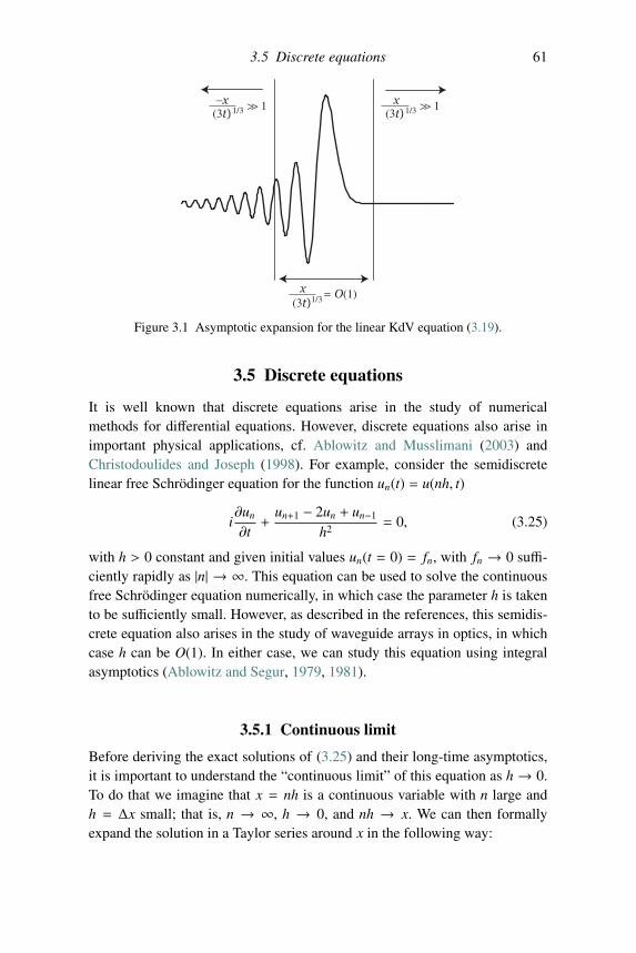
3.5 Discrete equations 61
x(3t)1/3 = O(1)
à 1x(3t)1/3à 1−x
(3t)1/3
Figure 3.1 Asymptotic expansion for the linear KdV equation (3.19).
3.5 Discrete equations
It is well known that discrete equations arise in the study of numericalmethods for differential equations. However, discrete equations also arise inimportant physical applications, cf. Ablowitz and Musslimani (2003) andChristodoulides and Joseph (1998). For example, consider the semidiscretelinear free Schrodinger equation for the function un(t) = u(nh, t)
i∂un
∂t+
un+1 − 2un + un−1
h2= 0, (3.25)
with h > 0 constant and given initial values un(t = 0) = fn, with fn → 0 suffi-ciently rapidly as |n| → ∞. This equation can be used to solve the continuousfree Schrodinger equation numerically, in which case the parameter h is takento be sufficiently small. However, as described in the references, this semidis-crete equation also arises in the study of waveguide arrays in optics, in whichcase h can be O(1). In either case, we can study this equation using integralasymptotics (Ablowitz and Segur, 1979, 1981).
3.5.1 Continuous limit
Before deriving the exact solutions of (3.25) and their long-time asymptotics,it is important to understand the “continuous limit” of this equation as h → 0.To do that we imagine that x = nh is a continuous variable with n large andh = Δx small; that is, n → ∞, h → 0, and nh → x. We can then formallyexpand the solution in a Taylor series around x in the following way:
62 Asymptotic analysis of wave equations
un±1(t) = u(nh ± h, t) = u(x ± h, t),
≈ u(x, t) ± hux(x, t) +h2
2uxx(x, t) + · · · .
Substituting this expansion into (3.25) and keeping O(1) terms leads to thecontinuous free Schrodinger equation,
iut + uxx = O(h2).
The initial conditions can be approximated in a similar manner, i.e., if un(t =0) = fn then in the continuous limit u(x, 0) = f (x).
3.5.2 Discrete dispersion relation
In analogy to the continuous case, we can find wave solutions to (3.25) thatserve as the basic building blocks for the solution. Similar to the constant coef-ficient continuous case, we can look for wave solutions (or special solutions)in the form
uns(t) = Zne−iωt,
where Z = eikh. Note that in the continuous limit i.e., as nh → x, we haveZn = eiknh → eikx, so this solution becomes ei(kx−ωt), i.e., the continuouswave solution. Substituting uns into (3.25) leads to the discrete dispersionrelation
ω +Z − 2 + 1/Z
h2= 0.
It is convenient to use Euler’s formula (Z + 1/Z)/2 = cos(kh) to rewrite thedispersion relation as
ω(k) =2[1 − cos(kh)]
h2. (3.26)
This is the dispersion relation for (3.25). Taking the continuous limit h → 0,k = O(1) fixed, and using a Taylor expansion leads to
ω(k) = k2,
which is exactly the dispersion relation for the continuous Schrodinger equa-tion. But it is important to note that the dispersion relations for the discrete andcontinuous problems are markedly different for large values of k.
3.5 Discrete equations 63
3.5.3 Z transforms and discrete Fourier transforms
The next step in the analysis is to represent the general solution as an integralof the special (wave) solutions, in analogy to the Fourier transform. This kindof representation is sometimes referred to as the Z transform. To understand itbetter, let us recall some properties of the Fourier transform. In the continuouscase, recall we have the pair
u(x) =1
2π
∫ ∞
−∞u(k)eikx dk,
u(k) =∫ ∞
−∞u(x)e−ikx dx.
Substituting the second into the first and interchanging the integrals yields
u(x) =1
2π
∫ ∞
−∞
[ ∫ ∞
−∞u(x′)e−ikx′ dx′
]eikx dk,
=1
2π
∫ ∞
−∞u(x′)
( ∫ ∞
−∞eik(x−x′) dk
)dx′,
=
∫ ∞
−∞u(x′)δ(x − x′) dx′,
= u(x), (3.27)
where we have used that the delta function satisfies
δ(x) =1
2π
∫ ∞
−∞eikx dk;
see Ablowitz and Fokas (2003) for more details.Now, the Z transform (ZT) and its inverse (IZT) are given by
un =1
2πi
∮C
u(z)zn−1 dz, (3.28)
u(z) =∞∑
m=−∞umz−m, (3.29)
where the contour C is the unit circle in the complex domain. In analogywith the Fourier transform (FT) pair, we substitute (3.29) into (3.28) and usecomplex analysis to get that
64 Asymptotic analysis of wave equations
un =1
2πi
∮C
[ ∞∑m=−∞
umz−m]zn−1 dz
=
∞∑m=−∞
um1
2πi
∮C
zn−m−1 dz
=
∞∑m=−∞
umδn,m = un, (3.30)
where the Kronecker delta δn,m is 1 when n = m and zero otherwise. Here
we have relied on the fact that1
2πi
∮zα dz, α integer, is equal to 1 only for a
simple pole, i.e., α = −1, and is otherwise equal to zero. Equation (3.30) usingcomplex analysis is the analog to (3.27) for the ZT.
In discrete problems it is convenient to put the ZT in a “Fourier dress”. Wecan do that by substituting z with k according to z = eikh. Since the contourof integration is the (counterclockwise) unit circle, k ranges from −π/h to π/hand z goes from −1 to 1. Thus, the ZT is transformed into the discrete Fouriertransform (DFT)
un =1
2πi
∫ π/h
−π/hu(z)eik(nh−h)iheikh dk =
h2π
∫ π/h
−π/hu(z)eiknh dk, (3.31)
using z(k) = eikh. In the continuous limit as h→ 0, we have hu(z) = hu(eikh)→u(k), nh→ x, un = u(nh)→ u(x) and we get the continuous FT
u(x) =1
2π
∫ ∞
−∞u(k)eikx dk.
For the IZT there is a corresponding inverse DFT (IDFT), which can also beobtained using z(k) = eikh:
hu(z) = h∞∑
m=−∞umz−m =
∞∑m=−∞
u(mh)e−i(mh)kh,
or, with mh → x, and noting that the Riemann sum tends to an integral withh = Δx:
u(k) =∫ ∞
−∞u(x)e−ixk dx.
Thus, in the continuous limit one obtains the continuous IFT.
3.5 Discrete equations 65
3.5.4 Asymptotics of the discrete Schrodinger equation
Using the DFT (3.31) replacing u(z) by u(z, t) = u0(z)e−iωt on the semidiscretelinear free Schrodinger equation (3.25) leads to the solution represented as
un(t) =h
2π
∫ π/h
−π/hu0(eikh)eiknhe−iω(k)t dk,
where from (3.26) we have that ω(k) = 2[1 − cos(kh)]/h2 and the initialcondition is u0(eikh) =
∑∞m=−∞ um(0)e−ikmh. Therefore, we get that
un(t) =h
2π
∫ π/h
−π/hu0(eikh)eiφ(k)t dk,
where
φ(k) = kχn − 2[1 − cos(kh)]h2
and χn = nh/t. Using the method of stationary phase we have that
φ′(k) =nht− 2 sin(kh)
h= 0,
from which the stationary points, k0, satisfy
sin(k0h) =nh2
2t. (3.32)
Note that the group velocity for the discrete equation is
vg = ω′(k) = 2 sin(kh)/h→ 2k
as h → 0 (k fixed), which is the group velocity corresponding to the contin-uous Schrodinger equation. In contrast to the continuous case, where vg(k) isunbounded, in the discrete case we now have that the group velocity is bounded
|vg| =∣∣∣∣∣2 sin(kh)
h
∣∣∣∣∣ ≤ 2h, (3.33)
where equality holds only when kh = ±π/2 (the degenerate case). This meansthat in contrast to the continuous Schrodinger equation, where information cantravel with an arbitrarily large speed, in the semidiscrete Schrodinger equationinformation can travel at most with a finite speed. This is typical in discreteequations. Only in the continuous limit h → 0, k fixed, does vg becomeunbounded.
We can further obtain that
−φ′′(k) = 2 cos(kh).
66 Asymptotic analysis of wave equations
Using (3.32) gives that at the stationary points
−φ′′(k0) = 2 cos(k0h),
= ±2√
1 − sin2(k0h),
= ±2
√1 −(− nh2
2t
)2,
= ±√
(2t)2 − (nh2)2
t.
Thus, using the stationary phase method, we obtain that
un(t) ∼∑
k0
hu0(k0)eiφ(k0)t+iμπ/4√2πt|φ′′(k0)| ,
where μ = sgn(φ′′(k0)). Note also that from (3.32), k0 is a function of n andfrom (3.32) there are generically two values of k0 for each n. Note that in thedegenerate case kh = ±π/2, or (nh)2 = (2t)2, one gets that φ′′ = 0, whichmeans that we need to take higher-order terms in the stationary phase method.
There are three regions that, in principle, can be studied: |nh2/2t| < 1,|nh2/2t| > 1, and near nh2/2t = ±1. The first, which is the most importantregion in this problem, is obtained by the stationary phase method given above.It gives rise to oscillations decaying like O(1/
√t). The “outside” region has
exponential decay (similar to the KdV equation as x/t → 0 and x/t > 0). Thematching region has the somewhat slower O(t−1/3) decay rate (this correspondsto kh ≈ π/2).
This discrete problem has behavior that is similar to the Klein–Gordonequation studied in Chapter 2,
utt − uxx + m2u = 0,
where the dispersion relation is given by ω(k) =√
k2 + m2 and the groupvelocity is bounded,
|vg| = |ω′(k)| =∣∣∣∣∣ k√
k2 + m2
∣∣∣∣∣ ≤ 1,
cf. equation (3.33).In a similar way one can also study the asymptotic analysis of the solution
to the doubly discrete Schrodinger equation,
ium+1
n − um−1n
Δt+
umn+1 − 2um
n + umn−1
h2= 0,
but we leave this as an exercise to the interested reader (see Exercise 3.5).
3.5 Discrete equations 67
3.5.5 Fully discrete wave equation and the CFL condition
Consider the wave equation
utt = c2uxx,
where c is a constant. Suppose we want to solve this equation using a standardsecond-order explicit centered finite-difference scheme, i.e.,
um+1n − 2um
n + um−1n
Δt2= c2
(umn+1 − 2um
n + umn−1
Δx2
), (3.34)
where Δx > 0,Δt > 0 are constant and umn = u(nΔx,mΔt). When using the
scheme (3.34), we are faced with the problem of numerical stability/instability.We can use the ZT in order to understand the origin of this issue as follows.Let us define the special (wave) solutions
umn s = ZnΩm,
where Z = eikh and Ω = e−iωt. Note that as in the continuous limit, substitutingum
n s into the scheme above leads to the “dispersion relation”
Ω − 2 +1Ω
Δt2= c2
Z − 2 +1Z
Δx2.
It is convenient to define
p =ΔtΔx
c
and rewrite the dispersion relation as a quadratic polynomial in Ω (or in Z) as
Ω2 −[2 + p2
(Z − 2 +
1Z
)]Ω + 1 = 0. (3.35)
In this way it is easier to spot the features of the dispersion relation. Indeed,since this relation is quadratic in Ω it has two roots Ω1,2 and can be written as
(Ω −Ω1)(Ω −Ω2) = Ω2 − (Ω1 + Ω2)Ω + Ω1Ω2 = 0.
Thus the sum of the two roots must be equal to the square brackets in (3.35)and the product of the two roots must be equal to 1. Hence, there are twocases to consider: either one root is greater than 1 and the other smaller, i.e.,|Ω1| < 1 and |Ω2| > 1 (the distinct-real root case), or both roots are equal to 1in magnitude. Defining b = 1+ p2(Z −2+1/Z)/2 = 1+ p2[cos(kh)−1], whereZ = eikh, we see that the discriminant, Δ, of (3.35) is given by Δ/4 = b2 − 1.Hence when |b| > 1 there are two distinct real-valued solutions and when|b| < 1 there are two complex roots. The double-root case corresponds to b = 1or kh = ±π/2.
68 Asymptotic analysis of wave equations
When |b| > 1 the solutions are unstable, because one of the roots is largerthan 1. From a numerical perspective this results in massively unstable growth,or “numerical ill-posedness”; note, the growth rate becomes arbitrarily large asΔt → 0,m → ∞ for fixed mΔt. The condition for stability |b| ≤ 1 correspondsto |1+ p2[cos(kΔx)− 1]| ≤ 1, which is satisfied by −2 ≤ p2[cos(kΔx)− 1] ≤ 0,or we can guarantee this inequality for all k if p2 ≤ 1, i.e.,
0 ≤ ΔtΔx
c ≤ 1 or 0 ≤ ΔtΔx≤ 1
c.
This condition was first discovered and named after Courant, Friedrichs, andLewy (Courant et al., 1928) and is often referred to as the CFL condition.
3.6 Burgers’ equation and its solution: Cole–Hopftransformation
In this section we study the solution of the viscous Burgers equation
ut + uux = νuxx, (3.36)
where ν is a constant, with the initial condition
u(x, 0) = f (x),
where f (x) is a sufficiently decaying function as |x| → ∞ and t > 0. It isconvenient to transform (3.36) using u = ∂ψ/∂x to get
ψt +12ψ2
x = νψxx,
where we assume ψ→ constant as |x| → ∞. Now let
ψ(x, t) = −2ν log φ(x, t), (3.37)
so
u(x, t) = −2νφx
φ(x, t), (3.38)
which is called the Cole–Hopf transformation (Cole, 1951; Hopf, 1950). Thisyields
(−2ν)φt
φ+
12
(−2ν)2
(φx
φ
)2= ν(−2ν)
⎡⎢⎢⎢⎢⎢⎣φxx
φ−(φx
φ
)2⎤⎥⎥⎥⎥⎥⎦ ,which simplifies to
φt = νφxx, (3.39)
the linear heat equation!
3.6 Burgers’ equation and its solution: Cole–Hopf transformation 69
Later in this book we will discuss the linearization and complete solution ofsome other important equations, such as the KdV equation, by the method ofthe inverse scattering transform (IST).
For Burgers’ equation, the solution is obtained by solving (3.39) and trans-forming back to u(x, t) via (3.38). To solve (3.39) we need the initial dataφ(x, 0), which are found from
−2νφx
φ(x, 0) = f (x)
or
φ(x, 0) = h(x) = C exp
(− 1
2ν
∫ x
0f (x′) dx′
). (3.40)
The constant C does not appear in (3.37) so without loss of generality we takeC = 1.
The solution to the heat equation with φ(x, 0) = h(x) can be obtained fromthe fundamental solution or Green’s function G(x, t):
φ(x, t) =∫ ∞
−∞h(x′)G(x − x′, t) dx′,
where it is well known that
G(x, t) =1√4πν
e−x2/4νt. (3.41)
We note that G(x, t) satisfies
Gt = νGxx,
G(x, 0) = δ(x).
Further, G(x, t) can be obtained by Fourier transforms
G(x, t) =1
2π
∫ ∞
−∞G(k, t)eikx dk,
G(k, t) =∫ ∞
−∞G(x, t)e−ikx dx.
Then
Gt = −νk2G
and with G(k, 0) = 1 we have
G(x, t) =1
2π
∫ ∞
−∞eikx−k2νt dk. (3.42)
The integral equation (3.42) can be evaluated by completing the square
G(x, t) = e−x2/4νt 12π
∫ ∞
−∞e−(k− x
2νt )2
dk =e−x2/4νt
2√πνt
,
70 Asymptotic analysis of wave equations
which yields (3.41). Thus the solution to the heat equation is
φ(x, t) =1√4πνt
∫ ∞
−∞h(x′)e−(x−x′)2/4νt dx′,
with φ(x, 0) = h(x) given by (3.40). Then the solution of the Burgers equationtakes the form
u(x, t) = −2νφx
φ=
∫ ∞−∞
x−x′t h(x′)e−(x−x′)2/4νt dx′∫ ∞
−∞ h(x′)e−(x−x′)2/4νt dx′
or using (3.40)
u(x, t) =
∫ ∞−∞
x−x′t e−Γ(x,t,x′)/2ν dx′∫ ∞
−∞ e−Γ(x,t,x′)/2ν dx′, (3.43)
with
Γ(x, t, x′) =(x − x′)2
2t+
∫ x′
0f (ζ) dζ.
In principle we can determine the solution at any time t by carrying out thequadrature in (3.43). But for general integrable functions f (x) the task is stillformidable and little qualitative information is obtained from (3.43) by itself.However, in the limit ν→ 0 we can recover valuable information. When ν→ 0we can use Laplace’s method (see Ablowitz and Fokas, 2003) to determine theleading-order contributions of the integral. We note that the minimum (in x′)of Γ(x, t, x′)/2ν, determined from
∂Γ
∂x′= Γ′(x′) = f (x′) − x − x′
t= 0,
gives the dominant contribution. An integral of the form
I(ν) =∫ ∞
−∞g(x′)e−Γ(x,t,x′)/2ν dx′,
can be evaluated as ν→ 0 by expanding Γ near its minimum x′ = ξ,
Γ(x, t, x′) = Γ(x, t, ξ) +12
(x′ − ξ)2Γ′′(x, t, ξ) + . . . ,
and
I(ν) ∼ν→0
√4πν
Γ′′(x, t, x′)e−Γ(x,t,ξ)/2ν.
Thus the solution u(x, t) from (3.43) is given, as ν→ 0, by
u(x, t) ∼x−ξ
t e−Γ(x,t,ξ)/2ν√
4πνΓ′′(x,t,ξ)
e−Γ(x,t,ξ)/2ν√
4πνΓ′′(x,t,ξ)
3.7 Burgers’ equation on the semi-infinite interval 71
or
u(x, t) ∼ x − ξt= f (ξ).
We recall that this is the exact solution to the inviscid Burgers equation
ut + uux = 0,
with u(x, 0) = f (x) in Section 2.6; we found u(x, t) = f (ξ) along x = ξ + f (ξ)tin regions where the solution is smooth. We remark that shocks can occur whenthere are multiple minima of equal value to Γ(x, t, ν), but we will not go intofurther details of that solution here.
3.7 Burgers’ equation on the semi-infinite interval
In this section we will discuss Burgers’ equation, (3.36), on the semi-infiniteinterval [0,∞).2 We assume u(x, t) → 0 rapidly as x → ∞ and at x = 0 themixed boundary condition
α(t)u(0, t) + β(t)ux(0, t) = γ(t), (3.44)
where α, β, γ are prescribed functions of t and we take for convenienceu(x, 0) = 0. It will be helpful to employ the Dirichlet–Neumann (DN) rela-tionship (often termed the DN map) associated with the heat equation (3.39)
φx(0, t) = − 1√νπ
∫ t
0
φτ(0, τ)√t − τ ,
= − 1√ν
D1/2t φ0(t), (3.45)
where φ0(t) = φ(0, t) and the “half-derivative” is defined as
D1/2t φ0(t) =
1√π
∫ t
0
φτ(0, τ)√t − τ .
Thus if we know φ(0, t) associated with (3.39) then (3.45) determines φx(0, t).Equation (3.45) can be found in many ways, e.g., via Laplace transforms(Ablowitz and Fokas, 2003): define the Laplace transform of φ(x, t) as
Φ(x, s) = L{φ} =∫ ∞
0φ(x, t)e−st dt;
then (3.39) implies
νΦxx − sΦ + 1 = 0,2 The analysis here follows the work of M. Hoefer developed for the “Nonlinear Waves” course
taught by M.J. Ablowitz in 2003.
72 Asymptotic analysis of wave equations
where we take φ(x, 0) = 1 with no loss of generality. Thus
Φ(x, s) = A(s)e−√
st x +
1s,
where we omitted the exponentially growing part. Then using (3.39) at x = 0,
Φxx(0, s) = L{
1νφt(0, t)
},
implies
A(s) =1√νsL {φt(0, t)} .
Hence
Φx(0, s) = − 1√νsL {φt(0, t)}
or by taking the inverse Laplace transform, using the convolution theorem, andL{1/√s} = 1/
√πt, we find (3.45).
The boundary condition (3.44) is converted to
α(t)φx
φ(0, t) + β(t)
[φxx
φ︸︷︷︸1νφtφ
−(φx
φ
)2](0, t) +
γ(t)2ν= 0
via the Hopf–Cole transformation (3.38). Or calling φ0(t) = φ(0, t) andusing (3.45) we have
α(t)D1/2
t φ0
φ0− β(t)√
ν
⎡⎢⎢⎢⎢⎢⎢⎣φ0t
φ0−⎛⎜⎜⎜⎜⎝D1/2
t φ0
φ0
⎞⎟⎟⎟⎟⎠2⎤⎥⎥⎥⎥⎥⎥⎦ (0, t) − γ(t)
2√ν= 0. (3.46)
We see that, in general, (3.46) is a nonlinear equation. However, in the caseof Dirichlet boundary conditions for Burgers’ equation, β(t) = 0, we findfrom (3.46) a linear integral equation of the Abel type for φ0:
D1/2t φ0 =
g(t)
2√νφ0,
where g(t) = γ(t)/α(t). Using D1/2t D1/2
t φ0(t) = φ0(t) − 1, i.e.,
1√π
∫ t
0
dτ1√t − τ1
· 1√π
∫ t
0
φ0,τ2 dτ2√t − τ2
=1π
∫ t
0dτ2 φ0,τ2
∫ t
τ2
dτ1√t − τ1
√τ1 − τ2︸���������������������︷︷���������������������︸
=π
= φ0(t) − 1
Exercises 73
(recall φ0(0) = 1), we have
φ0(t) = 1 +1
2√νπ
∫ t
0
g(t′)φ0(t′)√t − t′
dt′, (3.47)
which is an inhomogeneous weakly singular linear integral equation. Thisequation was obtained by a different procedure by Calogero and DeLillo(1989). Note, solving (3.47) gives φ(0, t), which combined with (3.40) allowsBurgers’ equation to be linearized via (3.39) with the Cole–Hopf transfor-mation (3.38). However, in general, the Hopf–Cole transformation does notlinearize the equation. Rather, we see that one has a nonlinear integral equa-tion (3.46) to study; but the number of variables has been reduced, from(x, t) to t.
Exercises
3.1 Analyze the long-time asymptotic solution of(a) iut + u4x = 0,(b) ut + u5x = 0, and(c) utt − uxx + m2u = 0,m > 0 constant.
3.2 Consider the equation
ut + cux = 0,
with c > 0 constant and u(x, 0) = f (x). Show that the solution is u =f (x − ct) and that this does not decay as t → ∞. Reconcile this with theRiemann–Lesbegue lemma.
3.3 Consider the linear KdV equation
ut + uxxx = 0.
Use the asymptotic analysis discussed in this chapter to analyze thebehavior of the energy inside each of the three asymptotic regions ast → ∞. At what speed does each propagate?
3.4 For the differential–difference, free Schrodinger equation,
i∂un
∂t+
un+1 − 2un + un−1
h2= 0,
with h > 0 constant, find the long-time solution in the regions |nh2/2t| >1 and near nh2/2t = ±1.
3.5 Consider the partial-difference equation,
ium+1
n − um−1n
Δt+
umn+1 − 2um
n + umn−1
Δx2= 0,
74 Asymptotic analysis of wave equations
with Δx > 0,Δt > 0 constant, assuming umn = u(n,m) and u(n, 0) and
u(n, 1) are given as initial conditions. Investigate the “long-time”, i.e.,m � 1, asymptotic solution.
3.6 Find a nonlinear PDE that is third order in space, first order in time thatis linearized by the Cole–Hopf transformation.
3.7 Use the Fourier transform method to solve the boundary value problem
uxx + uyy = −x exp(−x2),
u(x, 0) = 0,
−∞ < x < ∞, 0 < y < ∞,where u and its derivative vanish as y→ ∞. Hint: It is convenient to usethe inverse Fourier transform result: F −1
{1k f (k) dk
}=∫
f (x) dx.3.8 Solve the inhomogeneous partial differential equation
uxt = −ω sin(ωt), t > 0,
u(x, 0) = x, u(0, t) = 0.
3.9 Find the solution to Burgers’ equation (3.36) on the semi-infinite interval0 < x < ∞ with u(x, 0) = f (x) where f (x) decays rapidly as |x| → ∞and u(0, t) = g(t).
3.10 Solve the linear one-dimensional linear Schrodinger equation withquadratic potential (the “simple harmonic oscillator”)
iut = uxx − V0x2u,
with V0 > 0 constant and u(x, 0) = f (x) where f (x) decays rapidly as|x| → ∞. In what sense is the “ground state” (i.e., the lowest eigenvalue)the most important solution in the long-time limit? Hint: Use separationof variables.
4Perturbation analysis
In terms of the methods of asymptotic analysis, so far we have studied integralasymptotics associated with Fourier integrals that represent solutions of linearPDEs. Now, suppose we want to study physical problems like the propagationof waves in the ocean, or the propagation of light in optical fibers; the generalequations obtained from first principles in these cases are the Euler or Navier–Stokes equations governing fluid motion on a free surface and Maxwell’selectromagnetic (optical wave) equations with nonlinear induced polarizationterms. These equations are too difficult to handle using linear methods or,in most situations, by direct numerical simulation. Loosely speaking, thesephysical equations describe “too much”.
Mathematical complications often arise when one has widely separatedscales in the problem, e.g., the wavelength of a typical ocean wave is smallcompared to the ocean’s depth and the wavelength of light in a fiber is muchsmaller than the fiber’s length or transmission distance. For example, the typ-ical wavelength of light in an optical fiber is of the order of 10−6 m, whereasthe length (distance) of an undersea telecommunications fiber is of the order of10,000 km or 107 m, i.e., 13 orders of magnitude larger than the wavelength!Therefore, if we were to try solving the original equations numerically – andresolve both the smallest scales as well as keep the largest ones – we wouldrequire vast amounts of computer time and memory.
Yet it is imperative to retain some of the features from all of these scales,otherwise only limited information can be obtained. Therefore, before we canstudy the solutions of the governing equations we must first obtain useful andmanageable equations. For that we need to simplify the general equations,while retaining the essential phenomena we want to study. This is the roleof perturbation analysis and the reason why perturbation analysis often plays adecisive role in the physical sciences.
75
76 Perturbation analysis
In this chapter we will introduce some of the perturbation methods that willbe used later in physical problems. The reader can find numerous referenceson perturbation techniques, cf. Bender and Orszag (1999), Cole (1968), andKevorkian and Cole (1981). An early paper with many insightful principles ofasymptotic analysis (“asymptotology”) is Kruskal (1963). We will begin withsimpler “model” problems (ODEs) before discussing more complex physicalproblems.
4.1 Failure of regular perturbation analysis
Consider the ODEd2ydt2+ y = εy, (4.1)
where ε is a small (constant) parameter, i.e., |ε| � 1. Suppose we try to expandthe solution as
y = y0 + εy1 + ε2y2 + · · · ,
where the y j, j = 0, 1, 2, . . . , are assumed to be O(1) functions that are to befound. This is usually called regular perturbation analysis, because it is thesimplest and nothing out of the ordinary is used. Substituting this expansioninto (4.1) leads to an infinite number of equations, i.e., a perturbation seriesof equations. We group terms according to their power of ε. To O(1), i.e., forthose terms that have no ε before them, we get
O(1) : y0,tt + y0 = 0.
This is called the leading-order equation. Its solution, assumed to be real, calledthe leading-order solution, is conveniently given by
y0(t) = A0eit + A∗0e−it = A0eit + c.c.,
where A0 is a complex constant and c.c. denotes the complex conjugate ofthe terms to its left. Clearly, this solution does not have any ε in it, i.e., itcompletely disregards the εy term in (4.1). However, it may still be relativelyclose to the exact solution, because |ε| � 1. Two questions naturally arise:(a) How can we improve the approximation?(b) Is the solution we obtained a good approximation of the exact solution?
We can try to improve the approximation by going to the next order of theperturbation series, i.e., equating the terms that multiply ε1. This leads to
y1,tt + y1 = y0.
4.1 Failure of regular perturbation analysis 77
Since we already found y0, this is an equation for y1, the next order in theperturbation series (called the O(ε) correction). Substituting in the y0 abovegives
O(ε) : y1,tt + y1 = A0eit + c.c. (4.2)
Ignoring unimportant homogeneous solutions, the above equation has a solu-tion of the form
y1(t) = A1teit + c.c.,
where A1 is a constant, and substituting it into (4.2) leads to the condition
2i A1 = A0.
Therefore, we get that
y1(t) = − it2
A0eit + c.c.,
where we will omit additional terms due to the homogeneous solution. We cancontinue in a similar manner to obtain y2: the equation for y2 is found to be
y2,tt + y2 = y1;
we can guess a solution of the form y2 = A2t2eit + A3teit + c.c. and we obtain
8A2 = −A0, 8A3 = −iA0.
Using the first condition, 2iA1 = A0, we arrive at
y2 = −(
t2
8+ i
t8
)A0eit + c.c.
Let us inspect the solution we have so far obtained:
y = y0 + εy1 + ε2y2,
= (A0eit + c.c.) − ε( it
2A0eit + c.c.
)− ε2
((t2
8+ i
t8
)A0eit + c.c.
), (4.3)
= A0
(1 − ε it
2− ε2
(t2
8+
it8
) )eit + c.c. (4.4)
It is not difficult to convince ourselves that if we continue in the same fashionto include higher-order terms we will be adding higher-order monomials of tinside the parentheses. So long as t is O(1), our approximate solution should bequite close to the exact one. However, when t becomes large a problem ariseswith our solution. Indeed, when t = O(1/ε) the terms (εt)n inside the bracketsare of O(1), hence our formal solution is not asymptotic (i.e., the remainderof any finite number of terms is not smaller than the previous terms). It must
78 Perturbation analysis
be realized at this stage that this problem is not a feature of the exact solutionitself. Indeed, it is straightforward to obtain the exact solution of the linearequation (4.1):
yexact(t) = Aei√
1−ε t + c.c., (4.5)
where A is an arbitrary constant. This solution is finite and infinitely differ-entiable for any value of t. Moreover, from the binomial expansion
√1 − ε =
1 − ε/2 − ε2/8 + · · · and by further expanding the exponential we find theapproximation above; i.e., (4.4).
The failure is therefore on the part of the method we used. Inspecting thesolution (4.4) we see that the problem arises when t = O(1/ε) because theterms inside the parentheses become of the same order when t = O(1/ε).Hence the perturbation method breaks down because the higher-order termsare not small, violating our assumption. The violation is due to the terms thatgrow arbitrarily large with t. Such terms are referred to as “secular” or “res-onant”. Thus tneit is a secular term for any n > 1. If we trace our steps backwe see that the secular terms arise because the right-hand side of the non-homogeneous equations we obtain are in the kernels of the left-hand sides,e.g., in (4.2) the left-hand side Aeit is a solution of the homogeneous equationfor y1. This problem is inevitable when using the regular perturbation methodas outlined above. So how can we resolve it? This is where so-called “singular”perturbation methods enter the picture.
4.2 Stokes–Poincare frequency-shift method
We would like to find an approximate solution to (4.1) that is valid for large val-ues of t, e.g., up to t = O(1/ε). One perturbative approach is what we will callthe Stokes–Poincare or frequency-shift method; the essential ideas go back toStokes (see Chapter 5) and later Poincare. Although it does not work in everycase, it is often the most efficient method at hand. The idea of the frequency-shift method is explained below using (4.1) as an example. We define a newtime variable τ = ωt, where ω is called the “frequency”. Since d/dt = ωd/dτ,the equation takes the form
ω2 d2ydτ2+ y = εy.
We now expand the solution as before
y = y0 + εy1 + ε2y2 + · · · ,
4.2 Stokes–Poincare frequency-shift method 79
but also expand ω perturbatively as
ω = 1 + εω1 + ε2ω2 + · · · .
Substituting these expansions into the ODE and collecting the same powers ofε gives the leading-order equation
O(1) : y0,ττ + y0 = 0,
which is the same as we got using regular perturbation analysis. The leading-order solution is therefore
y0(τ) = Aeiτ + c.c.
The next-order equation is given by
O(ε) : y1,ττ + y1 = −2ω1y0,ττ + y0.
This equation has a term containing ω1, which is a modification of the regularperturbation analysis. Substituting the leading-order solution into the right-hand side leads to
y1,ττ + y1 = (1 + 2ω1)Aeiτ + c.c.
By choosing ω1 = −1/2, we eliminate the right-hand side and therefore avoidthe secular term in the solution. Without loss of generality, we choose the trivialhomogeneous solution, i.e., y1 = 0 (since we can “incorporate them” in theleading-order solution). We can continue in this fashion to obtain ω2; the next-order equation is given by
y2,ττ + y2 = −(2ω2 + ω
21
)y0,ττ + y1 − 2ω1y1.
Using y1 = 0 gives
y2,ττ + y2 = −(2ω2 + ω
21
)y0,ττ,
and choosing ω2 = −ω21/2 = −1/8 eliminates the secular terms; finally, we
choose y2 = 0.Let us inspect our approximate solution: the only non-zero part of y is y0,
but it contains ω to order O(ε2):
y(t) = Aeiτ + c.c. = Aeiωt + c.c.
= Aei(1+εω1+ε2ω2+··· )t + c.c. = Ae
i[1− ε
2− ε2
8 +···]t+ c.c.
80 Perturbation analysis
Hence we expect the solution to be valid for t = O(1/ε2). To verify this, let usexpand the square-root in the exact solution (4.5) in powers of ε:
yexact(t) = Aei√
1−ε t + c.c. = Aei[1− ε
2− ε2
8 +O(ε3)]
t+ c.c.,
so our exact and approximate solution agree to the first three terms in the expo-nent. Note that the remainder term in the exponent is O(ε3t), which is smallfor t = o(1/ε3). Furthermore, the approximate solution can be made validfor larger values of t by finding a sufficient number of terms in the frequencyexpansion. Note that the higher-order homogeneous solutions are chosen aszero (i.e, yk = 0 for k ≥ 1) and the higher non-homogeneities only change theamplitude, not the frequency, of the leading-order solution.
This example demonstrates the ease and efficiency of the frequency-shiftmethod. Unfortunately this method does not always work. For example, let usconsider the equation with a damping term
d2ydt2+ y = −εdy
dt
and repeat the analysis using the frequency-shift method. Defining τ = ωt asbefore leads to the equation
ω2 d2ydτ2+ y = −εωdy
dτ.
Expanding the solution and ω in powers of ε we get
(1 + εω1 + ε2ω2 + · · · )2 d2y
dτ2+ y = −ε(1 + εω1 + ε
2ω2 + · · · ) dydτ.
The leading-order solution is found to be
y0(τ) = Aeiτ + c.c.
The next-order equation is then
O(ε) : y1,ττ + y1 = −2ω1y0,ττ − y0,τ.
Substituting the leading-order solution into the right-hand side gives that
y1,ττ + y1 = 2ω1(Aeiτ + c.c.) − (iAeiτ + c.c.)
= (2ω1 − i)Aeiτ + (2ω1 + i)A∗e−iτ.
It may appear at first glance that we can avoid the secularity by choosing ω1 =
i/2; however, this is not so, because that only eliminates the terms that multiplyeiτ. Indeed, to eliminate the terms that multiply e−iτ we would need to chooseω1 = −i/2. In other words, we cannot choose ω1 consistently to eliminate allthe secular terms. Without eliminating the secular terms we are back to the
4.3 Method of multiple scales: Linear example 81
original problem, i.e., the solution will not be valid for t ∼ O(1/ε). Anothermethod is required.
The frequency-shift method usually works for conservative systems. Theaddition of the damping term results in a non-conservative (non-energyconserving) problem.
4.3 Method of multiple scales: Linear example
Since the frequency-shift method works in some cases but not in others, weintroduce the method of multiple scales, cf. Bender and Orszag (1999), Cole(1968) and Kevorkian and Cole (1981). The method of multiple scales has itsroots in the method of averaging, which have “rapid phases” and the otherterms are “slowly varying”, cf. Krylov and Bogoliubov (1949), Bogoliubovand Mitropolsky (1961); see also Sanders et al. (2009a).
The method of multiple scales is much more robust than the frequency-shiftmethod. It works for a wide range of problems and, in particular, for the prob-lems we will tackle here and for many problems that arise in nonlinear waves,as we will see later in this book. The idea is to introduce fast and slow vari-ables into the equation. Let us consider the damped example above, where thefrequency-shift method failed,
d2ydt2+ y = −εdy
dt. (4.6)
We can introduce the slow variable T = εt and consider y to be a functionof two variables: the “slow” variable T and the “fast” one t. We can thendenote y as
y = y(t,T ; ε),
where the ε is added here in order to stress that we will expand the solutionsin powers of ε. To be precise, we introduce two variables t = t and T = εt,however, we will omit the “∼” from t hereafter for notational convenience.
Using the chain rule for differentiation gives
dydt→ ∂y
∂t+ ε
∂y∂T
or in operator form
ddt→ ∂
∂t+ ε
∂
∂T
82 Perturbation analysis
and the equation is transformed into(∂
∂t+ ε
∂
∂T
)2y + y = −ε
(∂
∂t+ ε
∂
∂T
)y,
or
ytt + 2εytT + ε2yTT + y = −ε(yt + εyT ). (4.7)
It is important to note here that we have transformed an ODE into a PDE! Thus,formally, we have complicated the problem by this transformation, but thiscomplication is valuable, as we will now see. We now expand the solution as
y = y0 + εy1 + ε2y2 + · · · ,
substitute into the PDE (4.7), and collect like powers of ε. This leads to theleading-order equation
O(1) : y0,tt + y0 = 0.
Strictly speaking, this is a PDE since y depends on T as well. So the generalsolution is given by
y0(t,T ) = A(T )eit + c.c.,
where A(T ) is an arbitrary function of T . The next-order equation is foundto be
O(ε) : y1,tt + y1 = −2y0,tT − y0t.
Substituting the leading-order solution into the right-hand side gives that
y1,tt + y1 = −i(2AT + A)eit + c.c. (4.8)
As in the frequency-shift method, we would like to eliminate the secular terms.So we require that
2AT + A = 0. (4.9)
This ODE for A(T ) gives
A(T ) = A0e−T/2, (4.10)
where A0 is constant.Now we can choose the homogeneous solution y1 = 0, as in the frequency-
shift method. So far, our approximate solution is
y(t,T ) ∼ A(T )eit + c.c. = A0eit−T/2 + c.c.
In terms of the original variable t, this reads
y(t) ∼ A0eit−εt/2 + c.c. = A0e(i− ε2 )t + c.c. (4.11)
4.3 Method of multiple scales: Linear example 83
We can continue to obtain higher orders by allowing A(T ) to vary pertur-batively, in such a way as to avoid secular terms in the expansion of yk fork ≥ 1. Our method is to expand the equation for A(T ) without including addi-tional time-scales. Finding higher-order terms in the equation governing theslowly varying amplitude is usually what one desires in physical problems.However, care must be taken here, as we will see below. In the example above,we perturb (4.9) as
2AT + A = εr1 + ε2r2 + · · · . (4.12)
Substituting this into (4.8) shows that
y1,tt + y1 = −i(2AT + A)eit + c.c. = −iεr1eit + c.c.︸�����������︷︷�����������︸εR1
+O(ε2). (4.13)
Notice that there is an O(ε) residual term on the right-hand side. That termmust be added to the right-hand side of the next-order equation. When doingso we can choose y1 = 0 in this case (but see the next example!). Therefore,the O(ε2) equation corresponding to (4.7) is
y2,tt + y2 = −y0,TT − y0,T − 2y1,tT − y1,t − R1,
= −(ATT + AT )eit − ir1eit + c.c.,
where we have used y1 = 0 and R1 = (−ir1eit + c.c.), the coefficient of theO(ε) residual term from (4.13). In order to eliminate the secular terms in thisequation one requires that
r1 = i(ATT + AT ).
Substituting r1 in (4.12) leads to
(2AT + A) = iε(ATT + AT ). (4.14)
This is a higher-order equation, which at first glance may be a concern. Themethod for solving this equation, for ε � 1, is to solve (4.14) recursively;i.e., replace the ATT term with lower-order derivatives of A by using the equa-tion itself, while maintaining O(ε) accuracy. Let us see how that works in thisexample. Equation (4.14) implies that
AT = −12
A + O(ε). (4.15)
Differentiating with respect to T and using (4.15) to replace AT gives
ATT = −12
AT + O(ε) = −12
[− 1
2A + O(ε)
]+ O(ε) =
14
A + O(ε).
84 Perturbation analysis
We can now substitute ATT using this equation and substitute AT using (4.15)in (4.14) to find
(2AT + A) = −iε[14
A + O(ε) − 12
A + O(ε)].
Simplifying leads to the equation
AT = −12
(1 +
iε4
)A + O(ε2),
whose solution to O(ε) is
A(T ) = A(0)e−(12+
iε8 )T .
The above equation is a higher-order improvement of (4.10). Substituting A(T )and using T = εt in (4.11) gives
y ∼ A(0)e(1−ε2/8)ite−εt/2 + c.c. (4.16)
This approximate solution is valid for times t = O(1/ε2).We can now compare our result to the exact solution that can be found by
substituting ys = ert into (4.6). Doing so gives r2 + εr + 1 = 0 and therefore
yexact(t) = A(0)e(− ε
2+i2
√4−ε2
)t + c.c.
If we now expand the exponent in the exact solution in powers of ε, we find thatit agrees with the exponent in (4.16) to O(ε2), which is the order of accuracywe kept in the perturbation analysis:
−ε2+
i2
√4 − ε2 = −ε
2+ i
(1 − ε
2
8
)+ O(ε3).
This agrees with our approximate solution in (4.16).
4.4 Method of multiple scales: Nonlinear example
Below we give an example of using the method of multiple scales for thenonlinear ODE
d2ydt2+ y − εy3 = 0.
The first steps are similar to the previous example. We set T = εt and obtainthe equation
ytt + y + ε(2ytT − y3) + ε2yTT = 0.
4.4 Method of multiple scales: Nonlinear example 85
The leading-order equation and solution are the same as in the previousexample,
y0(t,T ) = A(T )eit + c.c.
The next-order equation is
O(ε) : y1,tt + y1 = −2y0,tT − y30.
Substituting the leading-order solution in the right-hand side and expandingthe nonlinear term leads to
y1,tt + y1 = −(2iAT eit + c.c.) + (Aeit + A∗e−it)3
= −(2iAT eit + c.c.) + (A3e3it + 3A2A∗eit + c.c.)
= −(2iAT − 3|A|2A)eit︸�������������������︷︷�������������������︸secular
+ A3e3it︸︷︷︸non-secular
+ c.c.
It is important to distinguish the terms that multiply eit from those that multiplye3it, because the former is a secular term, i.e., it satisfies the homogeneoussolution for y1, whereas the second one does not. Therefore, we must removethe secular terms, which multiply eit, but keep the non-secular terms, whichmultiply e3it, in the equation for y1 – the non-secular term results in a boundedcontribution to y1. To remove secularity, we require that
2iAT = 3|A|2A (4.17)
and the equation for y1 becomes
y1,tt + y1 = A3e3it + c.c. (4.18)
The solution of the (complex-valued) ODE (4.17) can be found by noting that|A|2 is a conserved quantity in time. One way to see this is by multiplying (4.17)by A∗, subtracting the complex conjugate, and integrating:
2iAT A∗ + 2iA∗T A = 3|A|2AA∗ − 3|A|2A∗A
and therefore i(|A|2)T = 0. Hence |A|2(T ) = |A|2(0) = |A0|2, where A0 is ourarbitrary constant. Using this conservation relation we can rewrite (4.17) as
2iAT = 3|A0|2A.
This is now a linear equation for A and its solution is given by
A(T ) = A0e−3i2 |A0 |2T = A0e−
3i2 |A0 |2εt.
86 Perturbation analysis
Note A(T ) depends on T = εt, so we can assume that A(T ) is constant whenintegrating the equation for y1 in (4.18). Assuming that y1 = Be3it + c.c. givesB = −A3/8, which is bounded, and therefore
y1(t) = −18
A3(T )e3it + c.c. + O(ε) = −18
A30e−
9i2 |A0 |2εte3it + c.c. + O(ε).
Finally, the perturbed solution we find is
y(t) = A0e(1− 3ε2 |A0 |2)it + εy1(t) + c.c.,
= A0e(1− 3ε2 |A0 |2)it − ε
8A3
0e−9i2 |A0 |2εte3it + c.c.
Inspecting our solution we note that the second term (the one multiplied byε) plays a minor role compared with the first term, since the amplitude of thesecond term is bounded and so remains O(ε) small relative to the first term forall values of t. We therefore focus our attention on the first term: its effectivefrequency is given by
Ω = 1 − 3ε2|A0|2. (4.19)
Therefore, when ε > 0, the additional frequency contribution decreases withamplitude |A0| (beyond the linear solution) and the period of oscillationsincreases (since T = 2π/Ω). This is sometimes called a “soft spring”, in anal-ogy with a spring whose period is elongated compared with a linear spring.Conversely, when ε < 0 the frequency increases and the period of oscillationsdecreases. This is called a “hard spring”.
Since the equation is conservative and there is only a (nonlinear) frequencyshift, this problem can also be done by the frequency-shift method. This is leftas an exercise.
4.5 Method of multiple scales: Linear and nonlinearpendulum
For our final application of multiple scales to ODEs, we will look at a nonlinearpendulum with a slowly varying length; see Figure 4.1. Newton’s second lawof motion gives
mly + mg sin(y) = 0
as the equation of motion, where m is the pendulum mass, g the gravitationalconstant of acceleration, and l the slowly varying length. This implies that
y + ρ2(εt) sin(y) = 0, (4.20)
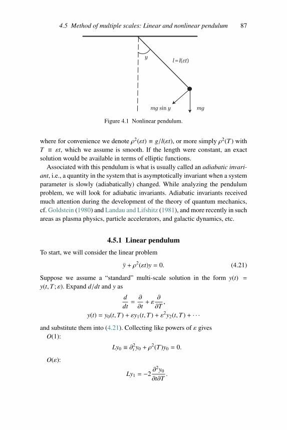
4.5 Method of multiple scales: Linear and nonlinear pendulum 87
Figure 4.1 Nonlinear pendulum.
where for convenience we denote ρ2(εt) ≡ g/l(εt), or more simply ρ2(T ) withT ≡ εt, which we assume is smooth. If the length were constant, an exactsolution would be available in terms of elliptic functions.
Associated with this pendulum is what is usually called an adiabatic invari-ant, i.e., a quantity in the system that is asymptotically invariant when a systemparameter is slowly (adiabatically) changed. While analyzing the pendulumproblem, we will look for adiabatic invariants. Adiabatic invariants receivedmuch attention during the development of the theory of quantum mechanics,cf. Goldstein (1980) and Landau and Lifshitz (1981), and more recently in suchareas as plasma physics, particle accelerators, and galactic dynamics, etc.
4.5.1 Linear pendulum
To start, we will consider the linear problem
y + ρ2(εt)y = 0. (4.21)
Suppose we assume a “standard” multi-scale solution in the form y(t) =y(t,T ; ε). Expand d/dt and y as
ddt=∂
∂t+ ε
∂
∂T,
y(t) = y0(t,T ) + εy1(t,T ) + ε2y2(t,T ) + · · ·and substitute them into (4.21). Collecting like powers of ε gives
O(1):
Ly0 ≡ ∂2t y0 + ρ
2(T )y0 = 0.
O(ε):
Ly1 = −2∂2y0
∂t∂T.
88 Perturbation analysis
The leading-order solution is
y0 = A(T ) exp(iρt) + c.c.
Notice that
∂T y0 = (AT + itρT ) exp(iρt) + c.c.
grows as t → ∞; i.e., it is secular! The problem is that we chose the wrong fasttime-scale. We modify the fast scale in y as follows:
y(t) = y(Θ(t), T ; ε),
where Θt = ω(εt) and ω will be chosen so that the leading-order solution is notsecular. Expand d/dt as
ddt= Θt
∂
∂Θ+ ε
∂
∂T= ω(T )
∂
∂Θ+ ε
∂
∂T.
A little care must be taken in calculating d2/dt2, since ω is a function of theslow variable: we get
d2
dt2=
(ω(T )
∂
∂Θ+ ε
∂
∂T
) (ω(T )
∂
∂Θ+ ε
∂
∂T
)= ω2 ∂2
∂Θ2+ ε
[2ω
∂2
∂Θ∂T+ ωT
∂
∂Θ
]+ ε2 ∂2
∂T 2. (4.22)
Substituting this into (4.21) and expanding y = y0 + εy1 + · · · we get the firsttwo equations
O(1):
ω2(T )∂2y0
∂Θ2+ ρ2(T )y0 = 0.
O(ε):
ω2(T )∂2y1
∂Θ2+ ρ2(T )y1 = −
(ωT
∂y0
∂Θ+ 2ω
∂2y0
∂T∂Θ
).
The leading-order solution is
y0 = A(T ) exp(iρ
ωΘ
)+ c.c.
To prevent secularity at this order we require that
∂y0
∂T= (AT + i(ρ/ω)T θA)ei(ρ/ω)θ
is bounded in θ. Hence we must take ω/ρ to be constant in order to removethe secular term. The choice of constant does not affect the final result, so
4.5 Method of multiple scales: Linear and nonlinear pendulum 89
for convenience we take ω = ρ. The order ε equation then becomes, aftersubstituting in the expression for y0,
ρ2(T )
(∂2y1
∂Θ2+ y1
)= −
(iρT AeiΘ + 2iATρeiΘ + c.c.
).
To remove secular terms, we require
2ρAT + AρT = 0,
2ρA∗T + A∗ρT = 0.
Multiplying the first equation by A∗, the second by A, and then adding, we findthat
∂
∂T
(ρ|A|2
)= 0 ⇒ ρ(T )|A(T )|2 = ρ(0)|A(0)|2 = E
ρ,
where E = ρ2A2 is related to the unperturbed energy E = y2/2 + ρ2y2/2,from (4.21); thus ρ(T )|A(T )|2 = E/ρ is constant in time. This is usually calledthe adiabatic invariant. Notice that ρ(T )|A(T )|2 is constant on the same time-scale as the length is being varied. Also, using separation of variables on theequation for AT ,
AT
A=−ρT
2ρ⇒ log(Aρ1/2) = constant ⇒ A(T ) =
C
ρ1/2(T )
where C is constant. Since ω = ρ,
Θ(t) =∫ t
0ρ(εt′) dt′ =
1ε
∫ εt
0ρ(s) ds.
The leading-order solution is then
y(t) ∼ C√ρ(εt)
exp
{iε
∫ εt
0ρ(s) ds
}+ c.c.
Alternatively, we can arrive at the same approximate solution using the so-called WKB method,1 cf. Bender and Orszag (1999). Instead of introducingmultiple time-scales, let T = εt and simply change variables in (4.21) to get
ε2 d2ydT 2+ ρ2(T )y(T ) = 0.
1 The WKB method is named after Wentzel, Kramers and Brillouin who used the methodextensively. However, these ideas were used by others including Jeffries and so is sometimesreferred to as the WKBJ method.
90 Perturbation analysis
If ρ were constant, the solution would be y = eiρ/ε + c.c. This suggests thatwe look for a solution in the form y ∼ eiφ(T ;ε)/ε + c.c. Using this ansatz, wefind
−φ2T + iεφTT + ρ
2 = 0.
We now expand φ as φ = φ0 + εφ1 + ε2φ2 + · · · to get the leading-order
equation
∂φ0
∂T= ±ρ(T )⇒ φ0 = ±
∫ T
0ρ(s) ds + μ0,
where μ0 is the constant of integration. The O(ε) equation is −2φ0Tφ1T +
iφ0TT = 0, so
∂φ1
∂T=
i2φ0TT
φ0T=
i2∂
∂Tlog |φ0T |,
which gives
φ1 =i2
log |φ0T | = i2
log(ρ).
Thus, in terms of the original variables:
y(t) ∼ exp[i (φ0 + εφ1) /ε
],
= exp
[iε
(∫ εt
0ρ(s) ds + μ0
)− 1
2log(ρ(εt))
]+ c.c.
Setting C = exp(iμ0/ε),
y(t) ∼ C√ρ(εt)
exp
[iε
∫ εt
0ρ(s) ds
]+ c.c.,
which is identical to the multiple-scales result.
4.5.2 Nonlinear pendulum
Now we will analyze the nonlinear equation, (4.20),
d2ydt2+ ρ2(T ) sin(y) = 0.
These and more general problems were analyzed by Kuzmak (1959), see alsoLuke (1966). We will see that this problem is considerably more complicatedthan the linear problem: multiple scales are required. As in the linear problem,
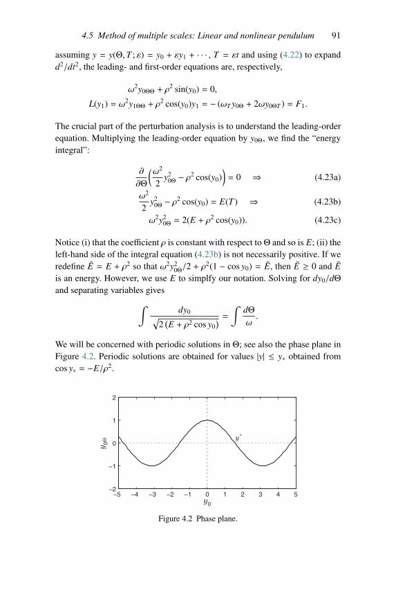
4.5 Method of multiple scales: Linear and nonlinear pendulum 91
assuming y = y(Θ,T ; ε) = y0 + εy1 + · · · , T = εt and using (4.22) to expandd2/dt2, the leading- and first-order equations are, respectively,
ω2y0ΘΘ + ρ2 sin(y0) = 0,
L(y1) = ω2y1ΘΘ + ρ2 cos(y0)y1 = − (ωT y0Θ + 2ωy0ΘT ) = F1.
The crucial part of the perturbation analysis is to understand the leading-orderequation. Multiplying the leading-order equation by y0Θ, we find the “energyintegral”:
∂
∂Θ
(ω2
2y2
0Θ − ρ2 cos(y0))= 0 ⇒ (4.23a)
ω2
2y2
0Θ − ρ2 cos(y0) = E(T ) ⇒ (4.23b)
ω2y20Θ = 2(E + ρ2 cos(y0)). (4.23c)
Notice (i) that the coefficient ρ is constant with respect to Θ and so is E; (ii) theleft-hand side of the integral equation (4.23b) is not necessarily positive. If weredefine E = E + ρ2 so that ω2y2
0Θ/2 + ρ2(1 − cos y0) = E, then E ≥ 0 and E
is an energy. However, we use E to simplfy our notation. Solving for dy0/dΘand separating variables gives∫
dy0√2(E + ρ2 cos y0
) = ∫ dΘω.
We will be concerned with periodic solutions in Θ; see also the phase plane inFigure 4.2. Periodic solutions are obtained for values |y| ≤ y∗ obtained fromcos y∗ = −E/ρ2.
−5 0 5−4 −3 −2 −1 1 2 3 4−2
−1
0
1
2
y0
y 0Θ
y*
Figure 4.2 Phase plane.
92 Perturbation analysis
The period of motion, P, is
P = ω∮
dy0√2(E + ρ2 cos y0
) ,where the loop integral is taken over one period of motion. Since cos(y0) iseven and symmetric, we can also calculate the period from
P = 4ω∫ y∗
0
dy0√2(E + ρ2 cos y0
) . (4.24)
Since the motion is periodic, for any integer n
y0(Θ + nP,T ) = y0(Θ, T ).
At this stage P is a function of T , thus
∂y0(Θ + nP,T )∂T
= n∂P∂T
∂y0(Θ, T )∂Θ
+∂y0(Θ, T )
∂T. (4.25)
For a well-ordered perturbation expansion, the first derivative∂y0(Θ + nP,T )/∂T must be bounded. However, from (4.25), ∂y0(Θ + nP,T )/∂T → ∞ as n → ∞. We can eliminate this divergence if we set ∂P/∂T = 0,i.e., we require the period to be constant. The choice of constant does notaffect the final result, so we can take P = 2π and then we have from (4.24),
ω = ω(E) =π
2∫ y∗
0
dy0√2(E + ρ2 cos y0
) . (4.26)
To find out how E varies, we must go to the next-order equation, namely,
Ly1 =[ω2∂2
Θ + ρ2(T ) cos(y0)
]y1 = F1 = − (ωT y0Θ + 2ωy0ΘT ) . (4.27)
We will not actually solve the O(ε) equation here, but instead we only need toderive a so-called solvability condition using a Fredholm alternative. We startby examining the homogeneous equation adjoint to (4.27): L∗W = 0, where L∗
is the adjoint to the operator L, with respect to the inner product
〈Ly,W〉 =∫ 2π
0(Ly) W dΘ = 〈y, L∗W〉;
integration by parts shows that L = L∗, i.e., the operator L is self-adjoint. Nowconsider
Ly1 =[ω2∂2
Θ + ρ2(T ) cos(y0)
]y1 = F1,
L∗W = LW = 0,
4.5 Method of multiple scales: Linear and nonlinear pendulum 93
where W is the periodic solution of the adjoint equation. There is another, non-periodic solution to the adjoint problem (obtained later for completeness); butsince we are only interested in periodic solutions, we do not need to considerit in the secularity analysis. Multiply the first equation by W, the second by y1,and subtract to find
ω2 ∂
∂Θ(Wy1Θ −WΘy1) = WF1.
Integrating this over one period and using the periodicity of the solution y1
gives ∫ 2π
0WF1 dΘ = 0 (4.28)
as a necessary condition for a periodic solution of the O(ε) equation to exist.This orthogonality condition must hold for the periodic solution, W, of thehomogeneous problem, which we will now determine. Operate on the leading-order equation with ∂/∂Θ to find
ω2y0ΘΘΘ + ρ2 cos(y0)y0Θ = 0,
i.e., y0Θ is a solution of LW = 0; hence we set W1 = y0Θ. This is the periodic,homogeneous solution. To find the non-periodic homogeneous solution operateon the leading-order equation with ∂/∂E to find
Ly0E = ω2y0EΘΘ + ρ
2 cos(y0)y0E = −(ω2)Ey0ΘΘ.
On the other hand, for any constant α,
L(αΘy0Θ) = ω2 ∂2
∂Θ2(αΘy0Θ) + ρ2 cos(y0)αΘy0Θ
= α[2ω2y0ΘΘ + Θ
(ω2y0ΘΘΘ + ρ
2 cos(y0)y0Θ
)].
The term in parentheses vanishes and we have
L(αΘy0Θ) = 2αω2y0ΘΘ.
Hence for the combination, y0E + αΘy0Θ:
L(y0E + αΘy0Θ) = L(y0E) + L(αΘy0Θ)
= −(ω2)
Ey0ΘΘ + 2αω2y0ΘΘ.
Thus, if we set α = ωE/ω,
L(y0E + αΘy0Θ) = 0
94 Perturbation analysis
and we have the second solution:
W2 = y0E +ωE
ωΘy0Θ,
cf. Luke (1966). This solution, however, is not generally periodic since ωE � 0in the nonlinear problem. We therefore need only one homogeneous solutionW1 in the Fredholm alternative (4.28). But the non-periodic solutions are usefulif one wishes to find the higher-order solutions. The solution y1 to Ly1 = F1
can be obtained by using the method of variation of parameters. The solvabilitycondition (4.28) now becomes ∫ 2π
0
∂y0
∂ΘF1 dΘ = 0,∫ 2π
0
∂y0
∂Θ(ωT y0Θ + 2ωy0ΘT ) dΘ = 0,
∂
∂T
∫ 2π
0ω
(∂y0
∂Θ
)2dΘ = 0.
We have therefore found an adiabatic invariant for this nonlinear problem:
A(T ) ≡ ω(T )∫ 2π
0
(∂y0
∂Θ
)2dΘ = A(0).
The invariant can also be written as
A(0) = ω(T )∫ 2π
0
(∂y0
∂Θ
)2dΘ = ω(T )
∮ (∂y0
∂Θ
)2 dy0dy0
dΘ
,
A(0) = 4ω(T )∫ y∗
0
∂y0
∂Θdy0,
= 4∫ y∗
0
√2(E + ρ2 cos(y0)
)dy0 ≡ F(E, ρ2). (4.29)
Thus E ≡ E(T ) is a function of ρ ≡ ρ(T ) in terms of the constA(0). Recall that(4.26) gives us ω ≡ ω(E(T )), in particular this leads to the convenient formula
ω = π/∂
∂EF(E, ρ2).
Hence the solution of the problem is determined in principle; i.e., these rela-tions give E = E(ρ(T )) = E(T ) and ω = ω(E(ρ(T ))) = ω(T ). So, we havedetermined the leading-order solution: y ∼ y0(Θ, E(T ), ω(T )).
4.5 Method of multiple scales: Linear and nonlinear pendulum 95
As an aside, the leading-problem can be solved explicitly in terms of ellip-tic functions. For completeness we now outline the method to do this. First,consider (
dudx
)2= P(u),
where P is a polynomial. If P is of second degree, we can express the solutionof the above equation in terms of trigonometric functions. If P is of third orfourth degree, the solution can be expressed in terms of elliptic functions (Byrdand Friedman, 1971).
Now recall the energy integral:
ω2
2y2
0Θ = E(T ) + ρ2 cos(y0).
To show that y0 can be related to elliptic problems, let z = tan(y0/2) so
dz/dy0 =12
sec2(y0/2). Then
dy0
dΘ=
dy0
dzdzdΘ= 2 cos2(y0/2)
dzdΘ
.
Using
cos(y0/2) =1√
1 + z2,
cos(y0) = 2 cos(y0/2)2 − 1 =1 − z2
1 + z2,
we substitute these results into the energy integral yielding
4ω2
2(1 + z2)2
(dzdΘ
)2=
(E + ρ2 1 − z2
1 + z2
),
and hence
2ω2
(dzdΘ
)2= (1 + z2)2E + ρ2(1 − z2)(1 + z2).
The right-hand side is a fourth-order polynomial and thus the solutions areelliptic functions. One can also transform the above integrals for ω and E intostandard elliptic integrals, see Exercise 4.6.
96 Perturbation analysis
Exercises
4.1 (a) Obtain the nonlinear change in the frequency given by (4.19) byapplying the frequency-shift method to the equation
d2ydt2+ y − εy3 = 0, |ε| � 1.
(b) Use the multiple-scales method to find the leading-order approxima-tion to the solution of
d2ydt2+ y − ε
(y3 +
dydt
)= 0, 0 < ε � 1.
(c) Find the next-order (first-order) approximation, valid for times t =o(1/ε2), to the solution of part (b).
4.2 Apply both the frequency-shift method and the method of multiple scales(|ε| � 1) to find the solution of:
(a)dAdt− iA + εA = 0,
(b)dAdt− iA + ε|A|2A = 0.
4.3 Use the method of multiple scales (|ε| � 1) to find an approximation tothe periodic solutions of:
(a)d4ydt4− y − εy = 0,
(b)d4ydt4− y − εy3 = 0.
4.4 Use the WKB method to find the leading-order approximation to thesolutions of
d4ydt4− ρ4(εt)y = 0, |ε| � 1.
4.5 Use the multiple-scale method to find:(a) the adiabatic invariant and leading-order solution of
d2ydt2− ρ2(εt)(y + y3) = 0, |ε| � 1;
(b) the leading-order approximation to the solution of
d2ydt2− ρ2(εt)(y + y3) = ε
dydt, 0 < ε � 1.
4.6 Considerd2ydt2+ ω2 sin y = 0,
where ω > 0 is a constant.
Exercises 97
(a) Find the energy integral by multiplying the equation with dy/dt andintegrating.
(b) Let y = 2 tan−1(z) (inverse tan-function) and find an equation for z.Solve the equation in terms of the Jacobi elliptic functions.
(c) Use part (b) to find all bounded solutions y.4.7 Suppose we are given
d2ydt2+ ρ2(εt) sin(y) = ε
dydt, 0 < ε � 1
Find the leading-order solution and contrast it with the asymptoticsolution for the pendulum discussed in Section 4.5.
5Water waves and KdV-type equations
Fluid dynamics is concerned with behavior on scales that are large comparedto the distance between the molecules that they consist of. Physical quanti-ties, such as mass, velocity, energy, etc., are usually regarded as being spreadcontinuously throughout the region of consideration; this is often termed thecontinuum assumption and continuum derivations are based on conservationprinciples. From these concepts, the equations of fluid dynamics are derived inmany books, cf. Batchelor (1967).
A microscopic description of fluids is provided by the Boltzmann equa-tion. When the average distance between collisions of the fluid moleculesbecomes small relative to the macroscopic dimensions of the fluid, the Boltz-mann equation can be simplified to the fluid equations (Chapman and Cowling,1970).
In this chapter, we focus on the most important results derived fromconservation laws and, in particular, how they relate to water waves.
We will use ρ = ρ(x, t) to denote the fluid mass density, v = v(x, t) is thefluid velocity, P is the pressure, F is a given external force, and ν∗ is the kine-matic viscosity that is due to frictional forces. In vector notation, the relevantequations of fluid dynamics we will consider are:• conservation of mass:
∂ρ
∂t+ ∇ · (ρv) = 0,
• conservation of momentum:
ρ
[∂v∂t+ (v · ∇) v
]= F − ∇P + ν∗Δv,
where Δ ≡ ∇2, is the Laplacian.1 We omit the equation of energy that describesthe temperature (T ) variation of the fluid, so an equation of state, such as
1 In three-dimensional Cartesian coordinates, the Laplacian is Δ ≡ ∂2/∂x2 + ∂2/∂y2 + ∂2/∂z2.
98
5.1 Euler and water wave equations 99
P = P(ρ,T ), is added to close the system of equations. These equations corre-spond to the first three moments of the Boltzmann equation. When ρ = ρ0 isconstant, the first equation then describes an incompressible fluid: ∇ · v = 0,also called the divergence equation. The divergence and the momentum equa-tions are often called the incompressible Navier–Stokes equations. The energyequation is not necessary to close this system of equations, which (in threedimensions) are four equations in four unknowns: v = (u, v,w) and P.
In this chapter, we will consider the free surface water wave problem,which (interior to the fluid) is the inviscid reduction (ν∗ = 0) of the aboveequations; these equations are called the Euler equations. Supplemented withappropriate boundary conditions, we have the Euler equations with a free sur-face. We will derive the shallow-water or long wave limit of this system anddiscuss certain approximate equations: the Korteweg–de Vries (KdV) equa-tion in 1 + 1 dimensions2 and the Kadomtsev–Petviashvili (KP) equation in2 + 1 dimensions.
5.1 Euler and water wave equations
For our discussion of water waves, we will use the above incompressibleNavier–Stokes description with constant density ρ = ρ0 and we will assumean ideal fluid: that is, a fluid with zero viscosity (ν∗ = 0). Thus, an ideal,incompressible fluid is described by the following Euler equations:
∇ · v = 0,
∂v∂t+ (v · ∇) v =
1ρ0
(F − ∇P) .
Suppose now that the external force is conservative, i.e., we can writeF = −∇U, for some scalar potential U. We can then write the momentumequation as
∂v∂t+ (v · ∇) v = −∇
(U + Pρ0
).
Using the vector identity
(v · ∇) v =12∇ (v · v) − v × (∇ × v) ,
gives
∂v∂t− v × (∇ × v) = −∇
(12
v · v + U + Pρ0
). (5.1)
2 The notation “n + 1 dimensions” means there are n space dimensions and one time dimension.
100 Water waves and KdV-type equations
Now define the vorticity to beω ≡ ∇×v, which is a local measure of the degree
to which the fluid is spinning; more precisely,12||∇ × v|| (note that ||v||2 = v · v)
is the angular speed of an infinitesimal fluid element. Taking the curl of the lastequation and noting that the curl of a gradient vanishes,
∂ω
∂t− ∇ × (v × ω) = 0.
Finally, using the vector identity ∇ × (F × G) = (G · ∇) F − (F · ∇) G +(∇ · G) F − (∇ · F) G for vector functions F and G and recalling that thedivergence of the curl vanishes, we arrive at the so-called vorticity equation:
∂ω
∂t= (ω · ∇)v − (v · ∇)ω or (5.2a)
DωDt= ω · ∇v, (5.2b)
where we have used the notation
DDt=∂
∂t+ (v · ∇)
to signify the so-called convective or material derivative that moves with thefluid particle (v = (u, v,w)). Hence ω = 0 is a solution; moreover, from (5.2b),it can be proven that if the vorticity is initially zero, then (if the solutionexists) it is zero for all times. Such a flow is called irrotational. Physically,in an ideal fluid there is no mechanism that will produce “local rotation” if thefluid is initially irrotational. Often it is a good approximation to assume thata fluid is irrotational, with viscosity effects occurring only in thin regions ofthe fluid flow called boundary layers. In this chapter, we will consider waterwaves and will assume that the flow is irrotational. In such circumstances, it isconvenient to introduce a velocity potential v = ∇φ. Notice that the vorticityequation (5.2b) is trivially satisfied since
∇ × (∇φ) = 0.
The Euler equations inside the fluid region can now also be simplified:
∇ · v = ∇ · ∇φ = Δφ = 0,
which is Laplace’s equation; it is to be satisfied internal to the fluid, −h < z <η(x, y, t), where we denote the height of the fluid free surface above the meanlevel z = 0 to be η(x, y, t) and the bottom of the fluid is at z = −h. See Figure 5.1on page 103.
Next we discuss the boundary conditions that lead to complications; i.e.,an unknown free surface and nonlinearities. We assume a flat, impenetrable
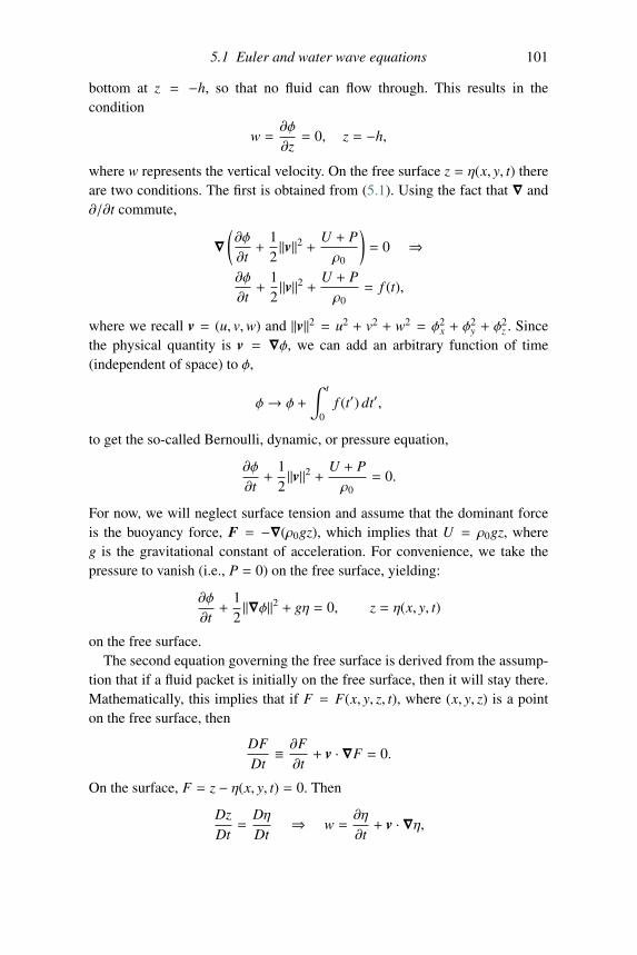
5.1 Euler and water wave equations 101
bottom at z = −h, so that no fluid can flow through. This results in thecondition
w =∂φ
∂z= 0, z = −h,
where w represents the vertical velocity. On the free surface z = η(x, y, t) thereare two conditions. The first is obtained from (5.1). Using the fact that ∇ and∂/∂t commute,
∇(∂φ
∂t+
12||v||2 + U + P
ρ0
)= 0 ⇒
∂φ
∂t+
12||v||2 + U + P
ρ0= f (t),
where we recall v = (u, v,w) and ||v||2 = u2 + v2 + w2 = φ2x + φ
2y + φ
2z . Since
the physical quantity is v = ∇φ, we can add an arbitrary function of time(independent of space) to φ,
φ→ φ +
∫ t
0f (t′) dt′,
to get the so-called Bernoulli, dynamic, or pressure equation,
∂φ
∂t+
12||v||2 + U + P
ρ0= 0.
For now, we will neglect surface tension and assume that the dominant forceis the buoyancy force, F = −∇(ρ0gz), which implies that U = ρ0gz, whereg is the gravitational constant of acceleration. For convenience, we take thepressure to vanish (i.e., P = 0) on the free surface, yielding:
∂φ
∂t+
12||∇φ||2 + gη = 0, z = η(x, y, t)
on the free surface.The second equation governing the free surface is derived from the assump-
tion that if a fluid packet is initially on the free surface, then it will stay there.Mathematically, this implies that if F = F(x, y, z, t), where (x, y, z) is a pointon the free surface, then
DFDt≡ ∂F∂t+ v · ∇F = 0.
On the surface, F = z − η(x, y, t) = 0. Then
DzDt=
DηDt
⇒ w =∂η
∂t+ v · ∇η,
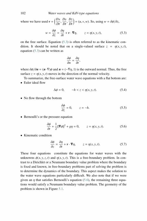
102 Water waves and KdV-type equations
where we have used v =(Dx
Dt,
DyDt,
DzDt
)= (u, v,w). So, using w = ∂φ/∂z,
w =∂φ
∂z=∂η
∂t+ v · ∇η, z = η(x, y, t), (5.3)
on the free surface. Equation (5.3) is often referred to as the kinematic con-dition. It should be noted that on a single-valued surface z = η(x, y, t),equation (5.3) can be written as
∂φ
∂n=∂η
∂t,
where ∂φ/∂n = (n·∇)φ and n = (−∇η, 1) is the outward normal. Thus, the freesurface z = η(x, y, t) moves in the direction of the normal velocity.
To summarize, the free-surface water wave equations with a flat bottom are:• Euler ideal flow
Δφ = 0, −h < z < η(x, y, t). (5.4)
• No flow through the bottom
∂φ
∂z= 0, z = −h. (5.5)
• Bernoulli’s or the pressure equation
∂φ
∂t+
12||∇φ||2 + gη = 0, z = η(x, y, t). (5.6)
• Kinematic condition
∂φ
∂z=∂η
∂t+ v · ∇η, z = η(x, y, t). (5.7)
These four equations constitute the equations for water waves with theunknowns φ(x, y, z, t) and η(x, y, t). This is a free-boundary problem. In con-trast to a Dirichlet or a Neumann boundary value problem where the boundaryis fixed and known, in free-boundary problems part of solving the problem isto determine the dynamics of the boundary. This aspect makes the solution tothe water wave equations particularly difficult. We also note that if we weregiven an η that satisfies Bernoulli’s equation (5.6), the remaining three equa-tions would satisfy a Neumann boundary value problem. The geometry of theproblem is shown in Figure 5.1.
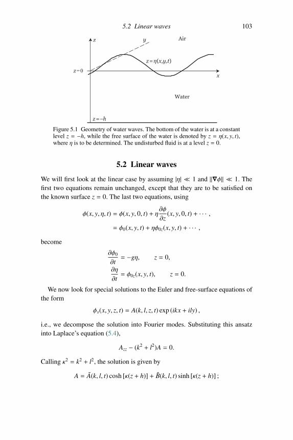
5.2 Linear waves 103
Figure 5.1 Geometry of water waves. The bottom of the water is at a constantlevel z = −h, while the free surface of the water is denoted by z = η(x, y, t),where η is to be determined. The undisturbed fluid is at a level z = 0.
5.2 Linear waves
We will first look at the linear case by assuming |η| � 1 and ||∇φ|| � 1. Thefirst two equations remain unchanged, except that they are to be satisfied onthe known surface z = 0. The last two equations, using
φ(x, y, η, t) = φ(x, y, 0, t) + η∂φ
∂z(x, y, 0, t) + · · · ,
= φ0(x, y, t) + ηφ0z(x, y, t) + · · · ,become
∂φ0
∂t= −gη, z = 0,
∂η
∂t= φ0z(x, y, t), z = 0.
We now look for special solutions to the Euler and free-surface equations ofthe form
φs(x, y, z, t) = A(k, l, z, t) exp (ikx + ily) ,
i.e., we decompose the solution into Fourier modes. Substituting this ansatzinto Laplace’s equation (5.4),
Azz − (k2 + l2)A = 0.
Calling κ2 = k2 + l2, the solution is given by
A = A(k, l, t) cosh [κ(z + h)] + B(k, l, t) sinh [κ(z + h)] ;
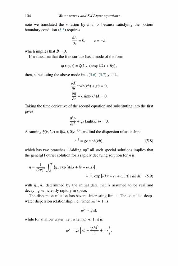
104 Water waves and KdV-type equations
note we translated the solution by h units because satisfying the bottomboundary condition (5.5) requires
∂A∂z= 0, z = −h,
which implies that B = 0.If we assume that the free surface has a mode of the form
η(x, y, t) = η(k, l, t) exp (ikx + ily) ,
then, substituting the above mode into (5.6)–(5.7) yields,
∂A∂t
cosh(κh) + gη = 0,
∂η
∂t− κ sinh(κh)A = 0.
Taking the time derivative of the second equation and substituting into the firstgives
∂2η
∂t2+ gκ tanh(κh)η = 0.
Assuming η(k, l, t) = η(k, l, 0)e−iωt, we find the dispersion relationship:
ω2 = gκ tanh(κh), (5.8)
which has two branches. “Adding up” all such special solutions implies thatthe general Fourier solution for a rapidly decaying solution for η is
η =1
(2π)2
� {η+ exp
[i(kx + ly − ω+t)
]+ η− exp
[i(kx + ly + ω−t)
]}dk dl, (5.9)
with η+, η− determined by the initial data that is assumed to be real anddecaying sufficiently rapidly in space.
The dispersion relation has several interesting limits. The so-called deep-water dispersion relationship, i.e., when κh � 1, is
ω2 � g|κ|,while for shallow water, i.e., when κh � 1, it is
ω2 � gκ
(κh − (κh)3
3+ · · ·
).
5.3 Non-dimensionalization 105
The leading term in the shallow-water dispersion relationship is ω2 � ghκ2.Alternatively, as discussed in earlier chapters, we have that to leading orderthe amplitude η satisfies the wave equation,
ηtt − c20ηxx = 0,
with a propagation speed c20 = gh. We will come back to this point when we
discuss the KdV equation later in this chapter.
5.3 Non-dimensionalization
To analyze the full equations, we will first non-dimensionalize them. By doingthis, it will be easier to compare the “size” of each term. This is convenientsince we will then be working with “pure” or dimensionless numbers. Forexample, a velocity can be large if measured in units of, say, microns per sec-ond but in units of light-years per hour it would be small. Indeed small or largein terms of coefficients in an equation are relative concepts and are meaningfulonly in a comparative sense. By studying non-dimensional equations we canmore easily decide which terms are negligible.
For shallow-water waves it is convenient to use the following non-dimensionalization:
x = λxx′, y = λyy′, z = hz′,
t =λx
c0t′, η = aη′, φ =
λxgac0
φ′,
where c0 =√
gh is the shallow-water wave speed, λx, λy are typical wave-lengths of the initial data (in the x or y direction), and a is the maximum ortypical amplitude of the initial data. The primed variables are dimensionless.For Laplace’s equation:
1λ2
xφ′x′x′ +
1λ2
yφ′y′y′ +
1h2φ′z′z′ = 0.
For the sake of notational simplicity, we will drop the primed notation so that
φzz +
(hλx
)2φxx +
(hλy
)2φyy = 0, −1 < z <
aηh.
The no-flow condition becomes
∂φ
∂z= 0, z = −1.
106 Water waves and KdV-type equations
Bernoulli’s equation becomes
φt +a
2h
⎡⎢⎢⎢⎢⎢⎣φ2x +
(λx
λy
)2φ2
y +
(λx
h
)2φ2
z
⎤⎥⎥⎥⎥⎥⎦ + η = 0, z =aηh.
And the kinematic condition becomes
ηt +ah
⎡⎢⎢⎢⎢⎢⎣φxηx +
(λx
λy
)2φyηy
⎤⎥⎥⎥⎥⎥⎦ = (λx
h
)2φz, z =
aηh.
Now we define the dimensionless parameters ε ≡ a/h, δ ≡ λx/λy, andμ ≡ h/λx: ε is a measure of the nonlinearity, or amplitude, of the wave; μis a measure of the depth relative to the characteristic wavelength, sometimescalled the dispersion parameter; and δ measures the size of the transverse vari-ations. In summary, the dimensionless equations for water waves propagatingover a flat bottom are• Euler ideal flow, Laplace’s equation
φzz + μ2φxx + μ
2δ2φyy = 0, −1 < z < εη.
• No flow through the bottom
∂φ
∂z= 0, z = −1.
• Bernoulli’s or the pressure equation
φt +ε
2
[φ2
x + δ2φ2
y +1μ2φ2
z
]+ η = 0, z = εη.
• Kinematic condition:
μ2[ηt + ε
(φxηx + δ
2φyηy
)]= φz, z = εη.
We note that the linear, or small-amplitude, case arises when ε� 1, μ∼O(1).Then the above equations reduce, by dropping terms of order ε, to the linearequations that are equivalent to those we analyzed earlier, i.e.,
φt + η = 0, z = 0,
μ2ηt = φz, z = 0,
but now in non-dimensional form.
5.4 Shallow-water theory
We will make some simplifying assumptions about the sizes of ε, μ, and δ inorder to obtain some interesting limiting equations:
5.4 Shallow-water theory 107
• We will consider shallow water waves (sometimes called long water waves).This regime corresponds to small depth relative to the water wavelength. Inour system of parameters, this corresponds to μ = h/λx � 1.
• We will also assume that the wavelength in the transverse direction is muchlarger than the propagation wavelength, so δ = λx/λy � 1.
• As before in the linear regime, we assume small-amplitude waves |ε| =a/h � 1. Recall that a similar assumption was made the Fermi–Pasta–Ulam(FPU) problem involving coupled nonlinear springs studied in Chapter 1.
• We will make the assumption of “maximal balance” (the small terms, i.e.,nonlinearity and dispersion, are of the same order) as was made in the con-tinuum approximation of the FPU problem to the Boussinesq model in orderto derive the KdV equation. We will do the same thing now by assumingmaximal balance with ε = μ2. This reflects a balance of weak nonlinearityand weak dispersion.
5.4.1 Neglecting transverse variations
First, we will consider the special case of no transverse waves and later wewill incorporate them into our model. Let us rewrite the fluid equations withthe simplifying assumptions ε = μ2 – this is our “maximal balance” assump-tion. Let us also consider the one-dimensional case, i.e., we remove the termsinvolving derivatives with respect to y. The four equations then become
εφxx + φzz = 0, −1 < z < εη (5.10a)
φz = 0, z = −1 (5.10b)
φt +ε
2(φ2
x +1εφ2
z ) + η = 0, z = εη (5.10c)
ε(ηt+εφxηx) = φz, z = εη. (5.10d)
These are coupled, nonlinear partial differential equations in φ and η witha free boundary, and are very difficult to solve exactly. We will use perturba-tion theory to obtain equations that are more tractable. We will asymptoticallyexpand φ as
φ = φ0 + εφ1 + ε2φ2 + · · · .
Substituting this expansion into (5.10a) gives
φ0zz + ε(φ0xx + φ1zz) + ε2(φ1xx + φ2zz) + · · · = 0.
108 Water waves and KdV-type equations
Equating terms with like powers of ε, we find that φ0zz = 0. This implies thatφ0 = A + B(z + 1), where A, B are functions of x, t. But the boundary condi-tion (5.10b) forces B = 0. Hence the leading-order solution for the velocitypotential is independent of z,
φ0 = A(x, t).
Proceeding to the next order in ε, we see that φ1zz = −Axx. Again using theboundary condition (5.10b),
φ1 = −Axx(z + 1)2/2.
As before, we absorb any homogeneous solutions that arise in higher-orderterms into the leading-order term (that is φ0). Similarly we find φ2 = Axxxx(z +1)4/4!. Thus, we have the approximation
φ = A − ε2
Axx(z + 1)2 +ε2
4!Axxxx(z + 1)4 + · · · , (5.11)
which is valid on the interval −1 < z < εη, in particular, right up to the freeboundary εη. This expansion can be carried out to any order in ε, but the firstthree terms are sufficient for our purpose.
Substituting (5.11) into Bernoulli’s equation (5.10c) along the free boundaryz = εη gives
At − ε2 Axxt(1 + εη)2 +ε2
4!Axxxxt(1 + εη)4 + · · ·
+ε
2
(Ax − ε2 Axxx(1 + εη)2 + · · ·
)2+
12
(−εAxx(1 + εη) + · · · )2 + η = 0.
Retaining only the first two terms leads to
η = −At +ε
2
(Axxt − A2
x
)+ · · · . (5.12)
Now let us do the same thing for the kinematic equation (5.10d). Substitutingin our expansion for φ and retaining the two lowest-order terms gives
εηt + ε2ηxAx = −εAxx(1 + εη) +
ε2
3!Axxxx + · · · . (5.13)
We wish to decouple the system of equations involving A and η. Since wehave an expression for η in terms of A, we substitute (5.12) into (5.13) andretain only the two lowest-order terms:
5.4 Shallow-water theory 109
ε(−Att +
ε
2(Axxtt − 2AxAxt) + ε
2(−AxtAx))
= −εAxx(1 − εAt) +ε2
3!Axxxx + · · · .
Dividing through by ε and keeping order ε terms gives
Att − Axx = ε(Axxtt
2− Axxxx
6− 2AxAxt − AxxAt
). (5.14)
Within this approximation, this equation is asymptotically the same as the oneBoussinesq derived in 1871, cf. Ablowitz and Segur (1981). Another form,equally valid up to order ε, is derived by noting that on the left-hand sideof (5.14) we have Att = Axx + O(ε). Then, in particular, we can take two xderivatives to obtain Axxtt = Axxxx + O(ε). Now we replace the Axxtt/2 term inthe above Boussinesq model to get
Att − Axx = ε(Axxxx
3− 2AxAxt − AxxAt
), (5.15)
which is still valid up to O(ε).Now we will make a remark about the linearized model. We have seen that
there are various ways to write the equation; for example,
Att − Axx = ε
(12
Axxtt − 16
Axxxx
)(5.16)
Att − Axx =ε
3Axxxx. (5.17)
But only one of these two gives rise to a well-posed problem. We can see thisfrom their dispersion relations: assume a wave solution A(x, t) = exp(i(kx−ωt))and substitute it into (5.16) (or recalling the correspondences k → −i∂x andω→ i∂t), then
−ω2 + k2 = ε
(ω2k2
2− k4
6
)=⇒ ω2 =
k2 + εk4/61 + εk2/2
.
Note ω2 > 0 and for very large k, ω2 ∼ k2/3 . If we substitute this back intoour wave solution, then we see that A(x, t) = exp(i(kx ± kt/
√3)) is bounded
for all time. But, if we do the same for (5.17), we get
−ω2 + k2 = εk4
3.
The large k limit of ω in this case is ω± ∼ ±i√εk2/
√3. Substituting the
negative root of ω into the wave solution we end up with
A(x, t) ∼ exp(ikx) exp(√
ε3 k2t).
110 Water waves and KdV-type equations
This solution blows up arbitrarily fast as k → ∞ so we do not have a conver-gent Fourier integral solution for “reasonable” (non-analytic) initial data (seealso the earlier discussion of well-posedness). If we wish to do numerical cal-culations then (5.16) is preferred as it is well-posed, as opposed to (5.17). Theill-posedness of (5.17) is due to the long-wave approximation. This is a com-mon difficulty associated with long-wave expansions; see also the discussionin Benjamin et al. (1972).
Nevertheless since there is still a small parameter, ε, in the equation, we canand should do further asymptotics on these equations. This will also removethe ill-posedness and is done in the next section.
First we make another remark about different Boussinesq models. We havederived an approximate equation for the leading term in the expansion of thevelocity potential φ (5.14) or (5.15). Combined with (5.11) it determines thevelocity potential, accurate to O(ε). We can also determine an equation forthe wave amplitude η. First we take an x derivative of (5.12) and then use thesubstitution u = Ax in (5.12)–(5.13) to find
Bernoulli: ηx = −ut +ε
2(uxxt − 2uux) + · · · , (5.18)
Kinematic: ηt = −ux + ε(−ηxu − ηux +
uxxx
6
)+ · · · . (5.19)
This is called the coupled Boussinesq model for η and u.On the other hand, by differentiating (5.19) with respect to t, and by
differentiating (5.18) with respect to x, we get
ηtt − ηxx = ε (−ηxtu − ηxut − ηtux − ηuxt
+uxxxt
6− uxxxt
2+
(u2)xx
2
)+ O(ε).
Now we use the relations ux = −ηt + O(ε) and ut = −ηx + O(ε) from thekinematic and Bernoulli equations, respectively, and make the replacement u =− ∫ x
−∞ ηt dx′. Hence we find
ηtt − ηxx = ε
[13ηxxxx + ηxt
∫ x
−∞ηt dx′ + η2
x + η2t
+ ηηxx +12∂2
∂x2
(∫ x
−∞ηt dx′
)2⎤⎥⎥⎥⎥⎥⎦ (5.20)
5.4 Shallow-water theory 111
= ε
[ηxxxx
3+∂
∂x
(ηt
∫ x
−∞ηt dx′ + ηηx
)+
12∂2
∂x2
(∫ x
−∞ηt dx′
)2⎤⎥⎥⎥⎥⎥⎦= ε
⎡⎢⎢⎢⎢⎢⎣ηxxxx
3+∂2
∂x2
⎛⎜⎜⎜⎜⎜⎝η2
2+
(∫ x
−∞ηt dx′
)2⎞⎟⎟⎟⎟⎟⎠⎤⎥⎥⎥⎥⎥⎦ . (5.21)
The last equation (5.21) is the Boussinesq model for the wave amplitude.If we omit the non-local term (which can be done via a suitable transfor-mation) (5.21) is reduced to the Boussinesq model discussed in Chapter 1[see (1.2), where η = yx].
5.4.2 Multiple-scale derivation of the KdV equation
Now let us return to the Boussinesq model for the velocity potential equa-tion (5.15) to do further asymptotics
Att − Axx = ε(Axxxx
3− 2AxAxt − AxxAt
). (5.22)
Assume an asymptotic expansion for A:
A = A0 + εA1 + · · · ;
substituting this expansion into (5.22) gives
A0tt + εA1tt − A0xx − εA1xx + O(ε2) = ε(A0xxxx
3−
−2A0xA0xt − A0xxA0t + O(ε)).
Equating the leading-order terms yields the wave equation: A0tt −A0xx = 0. Wesolved this equation earlier and found A0(x, t) = F(x − t) + G(x + t) where Fand G are determined by the initial conditions. Anticipating secular terms thatwill need to be removed in the next-order equation, we employ multiple scales;i.e., A0 = A0(ξ, ζ, T ):
A0 = F(ξ, T ) +G(ζ,T ),
where
ξ = x − t, ζ = x + t, T = εt.
These new variables imply
∂t = −∂ξ + ∂ζ + ε∂T and ∂x = ∂ξ + ∂ζ.
112 Water waves and KdV-type equations
Substituting the expressions for the differential operators into (5.22) leads to
((−∂ξ + ∂ζ + ε∂T )2 − (∂ξ + ∂ζ)2)A =
ε
((∂ξ + ∂ζ)4
3A − 2(∂ξ + ∂ζ)A(∂ξ + ∂ζ)(−∂ξ + ∂ζ + ε∂T )A
− (∂ξ + ∂ζ)2A(−∂ξ + ∂ζ + ε∂T )A
). (5.23)
First we will assume unidirectional waves and only work with the right-moving wave. So A0 = F(ξ, T ) for now. Substituting
A = A0 + εA1 + · · ·into (5.23) and keeping all the O(ε) terms we get
−4A1ξζ = 2FξT +13
Fξξξξ + 3FξξFξ.
This equation can be integrated directly to give
A1 ∼ −14
(2FT +
13
Fξξξ +32
F2ξ
)ζ + · · · ,
remembering that we absorb homogeneous terms in the A0 solution. In orderto remove secular terms, in particular the ζ term, we require that
2FT +13
Fξξξ +32
F2ξ = 0;
or, if we take a derivative with respect to ξ and make the substitution U = Fξ
then we have the Korteweg–de Vries equation
2UT +13 Uξξξ + 3UUξ = 0.
Next we discuss the more general case of waves moving to the left and right;hence A0 = F(ξ, T ) +G(ζ,T ), and we get the following expression for A1
− 4A1ξζ = 2(FξT −GζT ) +13
(Fξξξξ + +Gζζζζ)
+ 3(FξFξξ +13
FξξGζ − 13
GζζFξ −GζGζζ).
When we integrate this expression, secular terms arise from the pieces that arefunctions of ξ or ζ alone, not both. Removal of the secular terms implies thefollowing two equations
2FξT +13
Fξξξξ + 3FξξFξ = 0
−2GζT +13
Gζζζζ − 3GζζGζ = 0,
5.4 Shallow-water theory 113
which are two uncoupled KdV equations. Simplifying things a bit, we canrewrite the above two equations in terms of U = Fξ and V = Gζ :
2UT +13
Uξξξ + 3UUξ = 0 (5.24)
2VT − 13
Vζζζ + 3VVζ = 0. (5.25)
The solution A1 can be obtained by integrating the remaining terms. Since weare only interested in the leading-order asymptotic solution we need not solvefor A1.
Hence we have the following conclusion: asymptotic analysis of the fluidequations under shallow-water conditions has given rise to two Korteweg–deVries (KdV) equations, (5.24) and (5.25), for the right- and left-going waves.Given rapidly decaying initial conditions, we can solve these two PDEs forU and V by the inverse scattering transform (IST). The KdV equation hasbeen studied intensely and its IST solution is described in Chapter 9. Keepingonly the leading-order terms, we have an approximate solution for the velocitypotential
φ(x, z, t) ∼ A0(x, t) = F(x − t, εt) +G(x + t, εt),
=
∫ x−t
−∞U(ξ′, εt) dξ′ +
∫ x+t
−∞V(ζ′, εt) dζ′,
or for the velocity
u = φx = Fx +Gx + · · · = U + V + · · · .Using the Bernoulli equation (5.12), we have an approximate solution for
the wave amplitude of the free boundary
η(x, t) ∼ −A0t(x, t) ∼ Fξ(ξ, T ) −Gζ(ζ,T ) = U(x − t, εt) − V(x + t, εt).
Thus the wave amplitude η has right- and left-going waves that satisfy the KdVequation. Alternatively, we can derive the KdV equation directly by performingan asymptotic expansion in the η equation (5.21) though we will not do thathere. One can also proceed to obtain higher-order terms and corrections tothe KdV equation, though there is much more in the way of details that arerequired. We will not discuss this here.
5.4.3 Dimensional equations
In the previous section, we made our fluid equations non-dimensional forthe purpose of determining what terms are “small” in our approximation
114 Water waves and KdV-type equations
of shallow-water waves. Now that we have approximate equations (5.24)and (5.25), valid to leading order, we wish to understand the results indimensional units. We will now transform back to a dimensional equationfor (5.24).
Recall that we made two changes of variable. We first changed coordinatesx, t, η into primed coordinates x′, t′, η′ (though we immediately dropped theprimes). Then the independent variable substitutions ξ = x′ − t′ and T = εt′
were made. First, we remove the ξ and T dependence. Notice that
∂
∂t′U(ξ, T ) = −Uξ + εUT
∂
∂x′U(ξ, T ) = Uξ.
The above two expressions imply that ∂T = (∂t′ + ∂x′)/ε. Making the abovesubstitutions into (5.24), we get
2(Ut′ + Ux′ ) + ε
(13
Ux′x′x′ + 3UUx′
)= 0.
If we neglect left-traveling waves, V , then we have η′ ∼ U. Recalling our
original non-dimensionalization x = λxx′, t =λx
c0t′, ε = a/h and η = aη′, we
use ∂x′ = λx∂x and ∂t′ =λx
c0∂t to transform the previous expression in U to
2
(λx
c0
ηt
a+ λx
ηx
a
)+ ε
(λ3
x
3aηxxx +
3λx
a2ηηx
)= 0⇒
2
(ηt
c0+ ηx
)+
ah
(λ2
x
3ηxxx +
3aηηx
)= 0.
From maximal balance, we used ε = a/h = (h/λx)2 so we can simplify thenon-dimensional KdV equation (5.24) to the dimensional form
1c0ηt + ηx +
h2
6ηxxx +
32hηηx = 0, (5.26)
where c0 =√
gh, g is the gravitational constant of acceleration and h is thewater depth. This equation was derived by Korteweg and de Vries (1895).
Let us consider the linear part of (5.26)
1c0ηt + ηx +
h2
6ηxxx = 0.
5.4 Shallow-water theory 115
We will interpret the above equation in terms of the dispersion relation forwater waves [see (5.8)], noting κ2 = k2 + l2 with l = 0, so κ = k:
ω2 = gk tanh(kh) = gk
[kh − 1
3(kh)3 + · · ·
].
In shallow-water waves, kh � 1 so if we retain only the leading-order term inthe Taylor series expansion above, we have
ω = ±k√
gh = ±kc0.
This is the dispersion relation for the linear wave equation and c0 is the wavespeed. Retaining the next term in the Taylor series of tanh(kh) gives
ω ∼ ±k√
gh(1 − 13 (kh)2)
∼ ±k√
gh(1 − 16 (kh)2)
= ±(kc0 − 16 c0h2k3).
Now, we wish to see what linear PDE gives rise to the above dispersionrelation. Taking the positive root, replacing ω with i∂t and k with −i∂x, we find
i∂tη = c0(−i∂x)η − 16 c0h2(−i∂x)3η⇒
1c0ηt + ηx +
h2
6ηxxx = 0.
This is exactly the dimensional linear KdV equation (5.26)! To get thenonlinear term we used the multiple-scales method.
5.4.4 Adding surface tension
The model equations (5.4) through (5.7) do not take into account the effectsof surface tension. Actually only Bernoulli’s equation (5.10c) is affected bysurface tension. The modification is due to an additional pressure term fromsurface tension effects involving the curvature at the surface. We will not gothrough the derivation here: rather we will just state the result. First, recallBernoulli’s equation used so far
φt +12|∇φ|2 + gη = 0, (5.27)
116 Water waves and KdV-type equations
on z = η. Adding the surface tension term gives (cf. Lamb 1945 or Ablowitzand Segur 1981)
φt +12 |∇φ|2 + gη =
Tρ∇ ·⎛⎜⎜⎜⎜⎜⎝ ∇η√
1 + |∇η|2⎞⎟⎟⎟⎟⎟⎠
=Tρ
(ηxx
(1 + η2
y
)+ ηyy
(1 + η2
x
)− 2ηxyηxηy
)(1 + η2
x + η2y
) 32
(5.28)
on z = η where T is the surface tension coefficient. Retaining dimensions andkeeping linear terms that will affect the previous result to O(ε), we have:
φt +12|∇φ|2 + gη − T
ρ(ηxx + ηyy) = 0 z = η. (5.29)
Using (5.29) and the same asymptotic procedure as before, the correspondingleading-order asymptotic equation for the free surface is found to be
1c0ηt + ηx + γηxxx +
32hηηx = 0. (5.30)
The only difference between this equation and (5.26) is the coefficient γ of thethird-derivative term. This term incorporates the surface tension
γ =h2
6− T
2ρg=
h2
6
(1 − 3T
ρgh2
)=
h2
6(1 − 3T )
T =Tρgh2
.
Note (5.30) was also derived by Korteweg and deVries [see Chapter 1, equa-tion (1.4)], and we can see that, depending on the relative sizes of theparameters (in particular T < 1/3 or T > 1/3 ), γ will be positive or nega-tive. This affects the types of solutions and behavior allowed by the equationand is discussed later. In particular, when we include transverse waves, we willdiscover the Kadomtsev–Petviashvili (KP) equation.
5.4.5 Including transverse waves: The KP equations
Our investigation so far has been for waves in shallow water without transversemodulations. We will now relax our assumptions and include weak transversevariation.
First, let us look at the dispersion relation for water waves. Using thesame ideas as previously [see the discussion leading to (5.8)] the reader can
5.4 Shallow-water theory 117
verify that the dispersion relation in multidimensions (two space, one time) isgiven by
ω2 =
(gκ +
Tρκ3
)tanh(κh), (5.31)
where κ2 = k2 + l2; here k, l are the wavenumbers that correspond to the x- andy-directions, respectively. Recall that the wavelengths of a wave solution in theform αei(kx+ly−ωt) are λx = 2π/k and λy = 2π/l. We further assume that (recallour earlier definitions of scales)
δ =λx
λy=
lk� 1.
The above relation says that the wavelength in the y-direction is much largerthan the wavelength in the x-direction. This is what is referred to as weaktransverse variation.
We now derive the linear PDE associated with the dispersion relation (5.31)with weak transverse variation. Since we are still in the shallow-water regime,we have |hk| ∝ |h/λx| � 1 and we assume that κh = kh
√1 + l2/k2 � 1. Then
we expand the hyperbolic tangent term in a Taylor series to find
ω2 ≈(gκ +
Tρκ3
) (κh − 1
3(κh)3
)+ · · ·
= ghκ2
(1 +
Tgρκ2
) (1 − 1
3(κh)2
)+ · · ·
ω =√
gh k
(1 +
l2
k2
) 12(1 +
Tgρ
k2 + O(l2)
) 12
×(1 − 1
3(hk)2 + O(l2)
) 12.
Use of the binomial expansion and assuming |l/κ| � 1 and the maximalbalance relation l2 ∼ O(k4), we end up with (c0 =
√gh),
ωk ≈ c0
(k2 + k4
(T
2gρ− 1
6 h2
)+ 1
2 l2 + O(k6)
).
Now we can write down the linear PDE associated with this dispersion relationusing ω→ i∂t, k → −i∂x:
1c0ηtx + ηxx +
12ηyy +
h2
6(1 − 3T )ηxxxx = 0,
where we recall T = T/ρgh2. This is the linear Kadomtsev–Petviashvili (KP)equation. To derive the full nonlinear version, we must resort to multiple scales
118 Water waves and KdV-type equations
(Ablowitz and Segur, 1979, 1981). Though we will not do that here, if we takea hint from our work on the KdV equation, we can expect that the nonlinearpart of our equation will not change when we add in slow transverse (y) depen-dence. This is true and the full KP equation, first derived in 1970 (Kadomtsevand Petviashvili, 1970), in dimensional form is
∂x
(1c0ηt + ηx +
32hηηx + γηxxx
)+
12ηyy = 0, or
1c0ηt + ηx +
32hηηx + γηxxx = −1
2
∫ x
−∞ηyy dx′,
(5.32)
where γ =h2
6(1− 3T ). Usually in water waves surface tension is small and we
have T < 1/3 which gives rise to the so-called KPII equation
1c0ηxt + ηxx +
32h
(ηηx)x +h2
6ηxxxx = −1
2ηyy.
The equation termed the KPI equation arises when T = T/ρgh2 > 1/3;i.e., when surface tension effects are large. Alternatively, we can rescale theequation into non-dimensional form
∂x(ut + 6uux + uxxx) + 3σuyy = 0, (5.33)
where σ has the following meaning• σ = +1 =⇒ KPII: typical water waves, small surface tension,• σ = −1 =⇒ KPI: water waves, large surface tension.We note that if ηyy = 0 in (5.32) and we rescale, the resulting KP equation canbe reduced to the KdV equation in standard form
ut ± 6uux + uxxx = 0. (5.34)
The “+” corresponds to T < 1/3 whereas the “–” arises when T > 1/3.
5.5 Solitary wave solutions
As discussed in Chapter 1, the KdV and KP equations admit special, exactsolutions known as solitary waves. We also mentioned in Chapter 1 that asolitary wave was noted by John Scott Russell in 1834 when he observed awave detach itself from the front of a boat brought to rest. This wave evolvedinto a localized rounded hump of water that Russell termed the Great Wave ofTranslation. He followed this solitary wave on horseback as it moved along theUnion Canal between Edinburgh and Glasgow. He noted that it hardly changed
5.5 Solitary wave solutions 119
its shape or lost speed for over two miles; see Russell (1844); Ablowitz andSegur (1981); Remoissenet (1999) and www.ma.hw.uk/solitons. Today, scien-tists often use the term soliton instead of solitary wave for localized solutionsof many equations despite the fact that the original definition of a solitonreflected the fact that two solitary waves interacted elastically.
5.5.1 A soliton in dimensional form for KdV
Recall from above that the KdV equation in standard, non-dimensionalform, (5.34), can be written
ut ± 6uux + uxxx = 0, and ± when γ ≷ 0,
where
γ =h2
6(1 − 3T ).
A soliton solution admitted by the non-dimensional equation (5.34) is given by
u(x, t) = ±2β2 sech2(β(x ∓ 4β2t − x0)). (5.35)
Notice that the speed of the wave, c = 4β2, is twice the amplitude of the wave.Also, the “+” corresponds to γ > 0 that is physically a positive elevation wavetraveling on the surface like the one first observed by Russell. The “–” caseresults from γ < 0 and corresponds to a dip in the surface of the water. In fact,an experiment done only recently with high surface tension produced just sucha “depression” wave (Falcon et al., 2002).
The solitary wave or soliton solution equation (5.35) is in non-dimensionalform. We can convert this solution of the non-dimensional equation (5.34)directly to a solution of the dimensional equation (5.26). We will only con-sider here γ > 0; we leave it as an exercise to find the dimensional solitonwhen γ < 0. First consider (5.24) in the form
2U′T ′ +13
U′ξ′ξ′ξ′ + 3U′U′ξ′ ,
where we denote all variables with a prime. We will rescale the variablesappropriately. Assume the following transformation of coordinates
ξ′ = l1ξ, T ′ = l2T, U′ = l3U.
Then (5.24) becomes
2l2
UT +1
3l31Uξξξ + 3
l3l1
UUξ = 0.
120 Water waves and KdV-type equations
If we multiply the whole equation by l1/l3 then we get
2l1l2l3
UT +1
3l21l3Uξξξ + 3UUξ = 0.
To get (5.24) into standard form, (5.34), we set
2l1l2l3=
12
and1
3l21l3=
12.
One solution is (l1, l2, l3) = (1, 6, 2/3). Now our soliton solution takes the form
U′(ξ, T ) =4β2
3sech2
(β(ξ − 2
3β2T − x0)
).
Next use, ξ′ = x′ − t′ and T ′ = εt′ to find
U′(x′, t′) =4β2
3sech2
(β(x′ − (1 + 2
3β2ε)t′ − x0
).
The dimensional solution employs the following change of variables
η = aU′, x = λxx′, t =λx
c0t′.
Substituting this into our solution, we have
η(x, t) =4β2a
3sech2
(β
(xλx−(1 + 2
3β2ε) c0
λxt − x0
λx
)).
Now we use the relations a/h = ε, μ = h/λx, and μ2 = ε to write down thedimensional solution to the KdV equation in the form
η
h= 4
3εβ2 sech2
(β
h
√ε(x − (1 + 2
3β2ε)c0t − x0)
).
Note that both β and ε are non-dimensional numbers, and ε is related to thesize of a typical wave amplitude. Recall that a = |ηmax| and c2
0 = gh. The
excess speed beyond the long wave speed is2β2
3c0ε. Russell observed this as
well! Later, in 1871, Boussinesq found this relationship from the more generalpoint of view of weakly nonlinear waves moving in two directions. Boussinesqalso found KdV-type equations (Boussinesq, 1877). Korteweg and de Vriesfound this result in 1895 concentrating on unidirectional water waves. Theyalso found a class of periodic solutions in terms of elliptic functions and calledthem “cnoidal” functions (see also the discussion in Chapter 1).
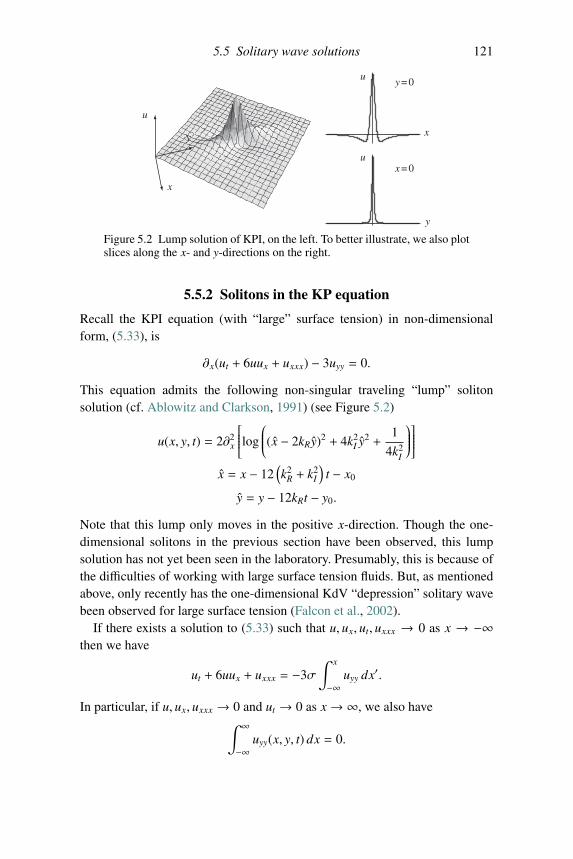
5.5 Solitary wave solutions 121
y = 0
x = 0
u
u
y
x
u
x
y
Figure 5.2 Lump solution of KPI, on the left. To better illustrate, we also plotslices along the x- and y-directions on the right.
5.5.2 Solitons in the KP equation
Recall the KPI equation (with “large” surface tension) in non-dimensionalform, (5.33), is
∂x(ut + 6uux + uxxx) − 3uyy = 0.
This equation admits the following non-singular traveling “lump” solitonsolution (cf. Ablowitz and Clarkson, 1991) (see Figure 5.2)
u(x, y, t) = 2∂2x
⎡⎢⎢⎢⎢⎣log
⎛⎜⎜⎜⎜⎝(x − 2kRy)2 + 4k2I y2 +
1
4k2I
⎞⎟⎟⎟⎟⎠⎤⎥⎥⎥⎥⎦x = x − 12
(k2
R + k2I
)t − x0
y = y − 12kRt − y0.
Note that this lump only moves in the positive x-direction. Though the one-dimensional solitons in the previous section have been observed, this lumpsolution has not yet been seen in the laboratory. Presumably, this is because ofthe difficulties of working with large surface tension fluids. But, as mentionedabove, only recently has the one-dimensional KdV “depression” solitary wavebeen observed for large surface tension (Falcon et al., 2002).
If there exists a solution to (5.33) such that u, ux, ut, uxxx → 0 as x → −∞then we have
ut + 6uux + uxxx = −3σ∫ x
−∞uyy dx′.
In particular, if u, ux, uxxx → 0 and ut → 0 as x→ ∞, we also have∫ ∞
−∞uyy(x, y, t) dx = 0.
122 Water waves and KdV-type equations
But if we give a general initial condition u(x, y, t = 0) = u0(x, y), it need notsatisfy this constraint at the initial instant. For the linearized version of theKP equation, one can show (Ablowitz and Villarroel, 1991) that if the initialcondition satisfies ∫ ∞
−∞u0(x, y) dx � 0,
nevertheless the solution obeys∫ ∞
−∞u(x, y, t) dx = 0, for all t � 0
and the function ∂u/∂t is discontinuous at t = 0. Ablowitz and Wang (1997)show why KP models of water waves lead to such constraints asymptoticallyand how a two-dimensional Boussinesq equation has an “initial value layer”that “smooths” the discontinuity in
∫uyy(x, y, t) dx.
5.5.3 KdV and related models
Suppose we consider the KdV equation in the form
ut + ux + ε(uxxx + αuux) = 0 (5.36)
where α is constant. First look at the linear problem and assume the wavesolution u ∼ exp(i(kx − ωt). The dispersion relation is then
ω = k − εk3,
which, for |k| � 1, implies ω ∼ −εk3. In particular, note that ω → −∞, whichcan present some numerical difficulties. One way around this issue is to use therelation ut = −ux + O(ε) to alter the equation slightly (Benjamin et al., 1972)
ut + ux + ε(−uxxt + αuux) = 0. (5.37)
Note that (5.36)–(5.37) are asymptotically equivalent to O(ε). But for large k,the dispersion relation for the linear problem is now
ω =k
1 + εk2∼ 1εk
for |k � 1. Numerically, (5.37) has some advantages over (5.36). But, we stillhave a “small” parameter, ε, in both equations so they are not asymptoticallyreduced. Alternatively, if we use the following transformation in (5.36), asindicated by multiple-scale asymptotics,
ξ = x − t, T = εt,
∂x = ∂ξ, ∂t = −∂ξ + ε∂T ,
5.5 Solitary wave solutions 123
then we get the equation
uT + uξξξ + αuuξ = 0, (5.38)
which has no direct dependence on the small parameter ε. Equation (5.38)is also useful for numerical computation since T = O(1) corresponds to t =O(1/ε).
Finally, recall the Fermi–Pasta–Ulam (FPU) model of nonlinear coupledsprings,
myi = k(yi+1 + yi−1 − 2yi) + α((yi+1 − yi)2 − (yi − yi−1)2) (5.39)
discussed in Chapter 1. In the continuum limit, use yi+1 = y(x) + hy′(x) +h2y′′(x)/2 + · · · , x = ih, to find
ω2ytt − h2yxx =h4
12yxxxx + 2αh3yxyxx + · · · ,
where we have used a dot to denoteddt
. Making the following substitutions
t = τ/hω, ω2 = k/m, ε = 2αh, and δ2ε = h2/12, where the last two equalitiesarise from the stipulation of maximal balance, we have
yττ − yxx = ε(δ2yxxxx + yxyxx). (5.40)
This is a Boussinesq-type equation and is also known to be integrable(Ablowitz and Segur, 1981; Ablowitz and Clarkson, 1991). The term integrablehas several interpretations. We will use the notion that if we can exactly lin-earize (as opposed to solving the equation via a perturbation expansion) theequation then we consider the equation to be integrable (see Chapters 8 and 9).Linearization or direct methods when applied to an integrable equation allowus to find wide classes of solutions.
Performing asymptotic analysis, in particular multiple scales on (5.40) withthe expansion
y ∼ y0 + εy1 + · · ·y0 = φ(X; T ), X = x − τ, T = ετ,
we find that, after removing secular terms (see also Chapter 1),
2φXT + φXφXX + δ2φXXXX = 0.
Or, if we make the substitution φX = u then we end up with the integrable KdVequation
uT +12 uuX +
δ2
2uXXX = 0.
124 Water waves and KdV-type equations
Another lattice equation, called the Toda lattice that is known to beintegrable, is given by
myi = ek(yi+1−yi) − ek(yi−yi−1).
If we expand the exponential and keep quadratic nonlinear terms, we getthe FPU model (5.39), which in turn asymptotically yields the KdV equa-tion. This further shows that the KdV equation (5.34) arises widely in appliedmathematics and the FPU problem itself is very “close” to being integrable.
5.5.4 Non-local system and the Benney–Luke equations
In a related development, a recent reformulation (see Ablowitz et al., 2006) ofthe fully nonlinear water wave equations with surface tension leads to twoequations for two unknowns: η and q = q(x, y, t) = φ(x, y, η(x, y, t)). Theequations are given by the following “simple looking” system∫ ∞
−∞
∫ ∞
−∞dxdyei(kx+ly)
(iηt cosh[κ(η + h)]
+1κ
(k, l) · ∇q sinh[κ(η + h)
])= 0 (I)
qt +12|∇q|2 + gη − (ηt + ∇q · ∇η)2
2(1 + |∇η|2)= σ∇ ·
⎛⎜⎜⎜⎜⎜⎝ ∇η√1 + |∇η|2
⎞⎟⎟⎟⎟⎟⎠ (II)
where (k, l)·∇q = kqx+lqy, κ2 = k2+l2, σ = T/ρwhere T is the surface tension
and ρ is the density; here η and derivatives of q are assumed to decay rapidlyat infinity. The first of the above two equations is non-local and is written in a“spectral” form.
The non-local equation satisfies the Laplace equation, the kinematic condi-tion and the bottom boundary condition. The second equation is Bernoulli’sequation rewritten in terms of the new variable q. These variables were intro-duced by Zakharov (1968) in his study of the Hamiltonian formulation of thewater wave problem. Subsequently they were used by Craig and co-workers(Craig and Sulem, 1993; Craig and Groves, 1994) in their discussion of theDirichlet–Neumann (DN) map methods in water waves. In this regard wenote:
ηt = φz − ∇φ · ∇η = ∇φ · �nwhere �n = (−∇η, 1) is the normal on y − η = 0. Thus finding q(x, y, t), η(x, y, t)yields ηt, which in turn leads to the normal derivative ∂φ/∂n; hence the DN
5.5 Solitary wave solutions 125
map is contained in the solution of the non-local system (I–II). Also, solvingequations (I)–(II) for η, q reduces to solving the remaining water wave equa-tion, Laplace’s equation (5.4), which is a linear problem due to the now fixedboundary conditions.
The non-local equation can be derived from Laplace’s equation, the kine-matic condition and the bottom boundary condition via Green’s identity (cf.Haut and Ablowitz, 2009). The essential ideas are outlined below. We alsomention that the reader will find valuable discussions of non-local systemswith auxiliary parameters in Fokas (2008). Fokas has made numerous impor-tant contributions in the study of such non-local nonlinear equations. We definean associated potential ψ(x, y, z) satisfying
Δψ(x, y, z) = 0, in D, ψy(x, y, z = −h) = 0. (5.41)
Then, from Green’s identity,
0 =∫
D(η)((Δψ) φ − (Δφ)ψ) dV
=
∫∂D(η)
(φ(∇ψ · n) − ψ(∇φ · n)) dS
where dV , dS are the volume and surface elements respectively, and n is theunit normal. It then follows that∫
ψ(x, y, η)ηt dxdy =∫
q(ψz(x, η) − ∇x,yψ(x, y, η) · ∇η
)dx dy, (5.42)
where we have used ηt = ∇φ ·�n, �n = (−∇η, 1) on the free surface as well as thebottom boundary condition and the condition |η| decaying at infinity.
We assume a solution of (5.41) can be written in the form
ψ(x, y, z) =∫
ξ(k, l)ψk,l(x, y, z)dkdl, ψk,l = ei(kx+ly) cosh[κ(z + h)].
Inserting ψk,l(x, y, z) into (5.42) yields∫R2
ei(kx+ly) cosh(κ(η + h)ηt dxdy
=
∫R2
q(ei(kx+ly)κ sinh(κ(η + h) − iei(kx+ly) cosh(κ(η + h) (k · ∇) η
)dx dy.
(5.43)
126 Water waves and KdV-type equations
Then, using
ei(kx+ly)κ sinh(κ(η + h) − iei(kx+ly) cosh(κ(η + h) ((k, l) · ∇) η
= −i∇ ·(eikx sinh(κ(η + h)
κ(k, l)
)in (5.43) and integrating by parts yields the non-local equation (I).
The second equation is essentially a change of variables. Differentiatingq(x, y, t) = φ(x, y, η(x, y, t), t) leads to
qx + φx + φzηx, qy = φy + φzηy.
These equations and
ηt + ∇φ · ∇η = φy
yield φx, φy, φz in terms of derivatives of η, q. Then from Bernoulli’s equationwith surface tension included, (5.28), we obtain equation (II).
If |η|, |∇q| are small then equations (I) and (II) simplify to the linearizedwater wave equations. Calling the Fourier transform η =
∫dx dyei(kx+ly)η,
and similarly for the derivatives of q, we find from equations (I) and (II)respectively
iηt cosh κh +k · ∇qκ
sinh κh = 0
qt + (g + σκ2)η = 0.
Then from these two equations we get
ηtt = −(gκ + σκ3) tanh κh η
which is the linearized water wave equation for η in Fourier space.We also remark that one can find integral relations by taking k, l → 0 in
equations (I) and (II) above. The first three, corresponding to powers k0, l0,k, l, are given by
∂
∂t
∫ ∞
−∞
∫ ∞
−∞dx dy η(x, y, t) = 0 (Mass)
∂
∂t
∫ ∞
−∞
∫ ∞
−∞dx dy(xη) =
∫ ∞
−∞
∫ ∞
−∞dx dy qx(η + h) (COMx)
∂
∂t
∫ ∞
−∞
∫ ∞
−∞dx dy(yη) =
∫ ∞
−∞
∫ ∞
−∞dx dy qy(η + h) (COMy).
They correspond to conservation of mass and the motion of the center of massin x, y respectively. The right-hand sides of (COMx, y) are related to the x, y-momentum respectively. Higher powers of k, l lead to “virial” type identities.
5.5 Solitary wave solutions 127
From the above system (I) and (II), one can also derive both deep- andshallow-water approximations to the water wave equations. In deep water, non-linear Schrodinger equation (NLS) systems result (see Ablowitz et al., 2006;Ablowitz and Haut, 2009b). In shallow water the Benney–Luke (BL) equa-tion (Benney and Luke, 1964), properly modified to take into account surfacetension, can be obtained.
To do this it is convenient to make all variables non-dimensional:
x′1 =x1
λ, x′2 = γ
x2
λ, t′ =
c0
λt , aη′ = η , q′ =
aλgc0
q , σ′ =σ
gh2
where c0 =√
gh and λ, a are the characteristic horizontal length and ampli-tude, and γ is a non-dimensional transverse length parameter. The equations
are written in terms of non-dimensional variables ε = a/h � 1, small-amplitude, μ = h/λ � 1 long waves; γ � 1, slow transverse variation.Dropping ′ we find∫
dxdyei(kx+ly)
(iηt cosh[κμ(1 + εη)] + sinh[κμ(1 + εη)]
(k, l) · ∇qκμ
)= 0 (5.44)
where (k, l) · ∇ = kqx + γ2lqy, κ2 = k2 + γ2l2.
In (5.44) we use
cosh[κμ(1 + εη)] ∼ 1 +μ2
2κ2, sinh[κμ(1 + εη)] ∼ μκ + μ
3
6κ3 + εμηκ.
Then, after inverse Fourier transforming, and with (k, l) → (i∂x, i∂y) we findfrom equations (I) and (II)(
1 − μ2
2Δ
)ηt +
(Δ − μ
2
6Δ2
)q + ε
(∇η · ∇q
)+ εηΔq = 0 (Ia)
η = −qt − ε2 |∇q|2 + σμ2Δη (IIa)
where Δ = ∂2x + δ
2∂2y , ∇η · ∇q = ηxqx + δ
2ηyqy, |∇q|2 =(q2
x + δ2q2
y
), and
σ = σ − 1/3.Eliminating the variable η we find, when ε, μ, δ � 1, the Benney–Luke (BL)
equation with surface tension included:
qtt − Δq + σμ2Δ2q + ε(∂t |∇q|2 + qtΔq) = 0, (5.45)
where σ = σ − 1/3. Alternatively, one can derive the BL system from theclassical water wave equations via asymptotic expansions as we have donepreviously for the Boussinesq models. The equations look somewhat differ-ent due to different representations of the velocity potential (see also theexercises).
128 Water waves and KdV-type equations
We remark that if we take the maximal balance ε = μ2 = δ2 then using mul-tiple scales the BL equation can be reduced to the unidirectional KP equation,which we have shown can be further reduced to the KdV equation if there isno transverse variation. Namely letting ξ = x − t, T = εt/2, w = qξ we find theKP equation in the form
∂ξ(wT − σwξξξ + 3(wwξ)) + wyy = 0.
Hence the non-local system (I)–(II) contains the well-known integrable waterwave reductions. We also note that higher-order asymptotic expansions of soli-tary waves and lumps can be obtained from equations (I) and (II) using thesame non-dimensionalization as we used for the BL equation. These expan-sions yield solitary waves close to their maximal amplitude (Ablowitz andHaut, 2009a, 2010)
Exercises
5.1 Derive the KP equation, with surface tension included, from the Benney–Luke (BL) equation (5.45): i.e., letting w = qξ, ε = μ2 = δ2, find
wTξ +(1/3 − T
)wξξξξ + wyy + (3wwξ)ξ = 0 (KP)
where T = εt, T = T/ρgh2, which is the well-known Kadomtsev–Petviashvili (KP) equation.
5.2 From the non-dimensional KP equation derived in Exercise 5.1, showthat the equation in dimensional form is given by
1c0ηxt +
32h
(ηηx)x + γηxxxx = −12ηyy
where γ = h2
6 (1 − 3T ).5.3 Find the dimensional form of a soliton solution to the KdV equation
when T > 1/3, i.e., γ < 0.5.4 Derive the equivalent BL equation for the velocity potential φ(x, y, 0, t)
from the classical water wave equations with surface tension included.5.5 Rewrite the lump solution given in this section in dimensional form.5.6 Given the “Boussinesq” model
utt − Δu + Δ2u + ||∇u||2 = 0,
make suitable assumptions about the size of terms, then rescale, andderive a corresponding KP-type equation.
Exercises 129
5.7 Given a “modified Boussinesq” model
utt − Δu + Δ2u + ||∇u||2+n = 0
with n a positive integer, make suitable assumptions about the size ofterms, then rescale, and derive a corresponding “modified KP”-typeequation.
5.8 Beginning with (5.22) assume right-going waves and obtain the KdVequation with a higher-order correction.
6Nonlinear Schrodinger models and water waves
A different asymptotic regime will be investigated in this chapter. Since nonlin-ear, dispersive, energy-preserving systems generically give rise to the nonlinearSchrodinger (NLS) equation, it is important to study this situation. In thischapter first the NLS equation will be derived from a nonlinear Klein–Gordonand the KdV equation. Then a discussion of how the NLS equation arisesin the limit of deep water will be undertaken. A number of results associ-ated with NLS-type equations, including Benney–Roskes/Davey–Stewartsonsystems, will also be obtained and analyzed.
6.1 NLS from Klein–Gordon
We start with the so-called “u-4” model, which arises in theoretical physics, orthe nonlinear Klein–Gordon (KG) equation – with two choices of sign for thecubic nonlinear term:
utt − uxx + u ∓ u3 = 0. (6.1)
Note, by multiplying the equation with ut we obtain the conservation ofenergy law
∂t
(u2
t + u2x + u2 ∓ u4/2
)− ∂x(2uxut) = 0
and hence the equation has a conserved density T1 = u2t + u2
x + u2 ∓ u4/2.Note the “potential” is proportional to V(u) = u2 ∓ u4/2, hence the term “u-4”model is used. We assume a real solution to (6.1) with a “rapid” phase andslowly varying functions of x, t:
u(x, t) = u(θ, X,T ; ε); X = εx, T = εt, θ = kx − ωt, |ε| � 1,
130
6.1 NLS from Klein–Gordon 131
where the dispersion relation for the linear problem in (6.1) is ω2 = 1 + k2.Based on the form of assumed solution the following operators are introducedin the asymptotic analysis:
∂t = −ω∂θ + ε∂T
∂x = k∂θ + ε∂X .
The weakly nonlinear asymptotic expansion
u = εu0 + ε2u1 + ε
3u2 + · · ·,and the differential operators are substituted into (6.1) leading to[
(−ω∂θ + ε∂T )2 − (k∂θ + ε∂X)2]
u + u ∓ u3 = 0
or [(ω2 − k2)∂2
θ − ε(2ω∂θ∂T + 2k∂θ∂X)+ ε2(∂2
T − ∂2X
)](εu0 + ε
2u1 + · · · )++ (εu0 + ε
2u1 + · · · ) ∓ (εu0 + ε2u1 + · · · )3 = 0.
We will find the equations up to O(ε3); the first two are:
3O(ε) : (ω2 − k2)∂2θu0 + u0 = 0
⇒ u0 = Aeiθ + c.c.
O(ε2) : (ω2 − k2)∂2θu1 + u1 = (2ωiAT + 2kiAX)eiθ + c.c.
where c.c. denotes the complex conjugate. Note: throughout the discussion wewill use the dispersion relation ω2 − k2 = 1. In order to remove secular terms,we require that the coefficient on the right-hand side of the O(ε2) equationbe zero. This leads to an equation for A(X,T ) that, to go to higher order, wemodify by using the asymptotic expansion
2i(ωAT + kAX) = εg1 + ε2g2 + · · · . (6.2)
The quantity A(X,T ) is often called the slowly varying envelope of the wave.As usual, we absorb the homogeneous solutions into u0 so u1 = 0. Now let uslook at the next-order equation
O(ε3) : (ω2 − k2)∂2θu2 + u2 = −(ATT − AXX)eiθ + c.c.
± (Aeiθ + A∗e−iθ)3 + g1eiθ + c.c.
In order to remove secular terms, we eliminate the coefficient of eiθ. Thisimplies
g1 = (ATT − AXX) ∓ 3A2A∗.
132 Nonlinear Schrodinger models and water waves
Combining the above relation with the asymptotic expansion in (6.2) we have
2iω(AT + ω′(k)AX) = ε(ATT − AXX ∓ 3|A|2A), (6.3)
where we used the dispersion relation to find ω′(k) = k/ω. After removing thesecular terms, we can solve the O(ε3) equation for u2 giving
u2 = ∓18
A3e3iθ + c.c.
Note, in (6.3), we can transform the equation for A and remove the ε (groupvelocity) term. To do this, we change the coordinate system so that we aremoving with the group velocity ω′(k) – sometimes this is called the group-velocity frame:
ξ = X − ω′(k)T ∂T = −ω′(k)∂ξ + ε∂τ
τ = εT = ε2t ∂X = ∂ξ.
Now, we use (6.3) to find
2iω(−ω′Aξ + εAτ + ω′Aξ) = ε((ω′)2Aξξ − Aξξ ∓ 3|A|2A) + O(ε2).
We can simplify this equation by using the dispersion relation as follows:ω′ = k/ω and
ω′′ =ω − ω′kω2
=1ω− kω′
ω2=
1ω
[1 − (ω′)2
],
to arrive at the nonlinear Schrodinger equation in canonical form:
iAτ +ω′′
2Aξξ ± 3
2ω|A|2A = 0. (6.4)
It is important to note that, like the derivation of the Korteweg–de Vriesequation in the previous chapter, the small parameter, ε, has disappeared fromthe leading-order NLS equation. The NLS equation is a maximally balancedasymptotic system.
The behavior of (6.4) depends on the plus or minus sign. The NLS equationwith a “+”, here
ω′′ =ω2 − k2
ω3=
1ω3,
so ω′′/ω > 0. The NLS with a “+” sign is said to be “focusing” and we willsee gives rise to “bright” solitons. Bright solitons have a localized shape anddecay at infinity. With a “−”, NLS is said to be “defocusing” and we willsee admits “dark” soliton solutions. Dark solitons have a constant amplitudeat infinity. The terminology “bright” and “dark” solitons is typically used in
6.2 NLS from KdV 133
nonlinear optics. We will discuss these solutions later, and nonlinear optics ina subsequent chapter.
In our derivation of NLS, we transformed our coordinate system to coincidewith the group velocity of the wave. An alternative form, useful in nonlinearoptics and called the retarded frame, is
t′ = T − 1ω′(k)
X ∂T = ∂t′
χ = εX ∂X = − 1ω′∂t′ + ε∂χ.
Next, we substitute the above relations into (6.3) to find
2iω
(At′ + ω
′[(−1ω′
)At′ + εAχ
])= ε
(At′t′ − 1
(ω′)2At′t′ ∓ 3|A|2A
).
Again we simplify this equation into a nonlinear Schrodinger equation
iAχ +ω′′
2(ω′)3At′t′ ± 3
2ωω′|A|2A = 0. (6.5)
Note that in the above equation, the “evolution” variable is χ and the “spatial”variable is t′.
6.2 NLS from KdV
We can also derive the NLS equation from the KdV equation asymptoti-cally for small amplitudes. To do that, we expand the solution of the KdVequation
ut + 6uux + uxxx = 0
as
u = εu0 + ε2u1 + ε
3u2 + · · · ,where for convenience the assumption of small amplitude is taken throughthe expansion of u rather than in the equation itself. Since the nonlinearterm, uux, is quadratic rather than cubic, it will turn out that the reductionto the NLS equation requires more work than in the KG equation. As wewill see, in this case one needs to remove secularity at one additional powerof ε, which in this case is O(ε3). Another difficulty is manifested by theneed to consider a mean term in the solution. Indeed, the equation to leadingorder is
u0,t + u0,xxx = 0,
134 Nonlinear Schrodinger models and water waves
whose real solution is given by
u0 = A(X,T )eiθ + c.c. + M(X,T ), (6.6)
where again T = εt and X = εx are the slow variables, θ = kx − ωt is the fastvariable, with the dispersion relation ω = −k3, and M(T, X) is a real, slowlyvarying, mean term, i.e., it corresponds to the coefficient of einθ with n = 0. Thequantity A(X,T ) is the slowly varying envelope of the rapidly varying wavecontribution. As we will see, in this case the mean term turns out to be O(ε),however, that is not always the case.1 Note that the addition of the complexconjugate (“c.c.”) in (6.6) corresponds to the first term and not to the meanterm, which is real-valued.
Substituting ∂t = −ω∂θ + ε∂T and ∂x = k∂θ + ε∂X in the KdV equationleads to
(−ω∂θ + ε∂T )u + 6u(k∂θ + ε∂X)u + (k∂θ + ε∂X)3u = 0.
Using the above expansion for the solution, u = εu0 + ε2u1 + ε
3u2 + · · ·gives
(−ω∂θ + ε∂T )(εu0 + ε2u1 + ε
3u2 + · · · )+ 6(εu0 + ε
2u1 + ε3u2 + · · · )(k∂θ + ε∂X)(εu0 + ε
2u1 + ε3u2 + · · · )
+ (k∂θ + ε∂X)3(εu0 + ε2u1 + ε
3u2 + · · · ) = 0.
The leading-order solution of Lu0 = 0, L defined below, is given by (6.6).We recall that the dispersion relation for the exponential term is given byω(k)=− k3. The O(ε2) equation is
Lu1 = −u0,T − 3k2u0,θθX − 6u0ku0,θ
= (−AT eiθ + c.c.) − MT + (3k2AXeiθ + c.c.)
− 6(Aeiθ + c.c.) + M)(Aikeiθ + c.c.),
where we have defined the linear operator (using ω = −k3),
Lu = k3(uθ + uθθθ).
Thus, we rewrite the O(ε) equation as
Lu1 = (−AT − ω′AX − 6iMkA)eiθ + c.c. − 6(ikA2e2iθ + c.c.) − MT ,
where we have used the dispersion relation, from which one gets thatω′(k)=− 3k2. In order to remove secular terms we note that such terms arise
1 For example, in finite-depth water waves the mean term is O(1) (Benney and Roskes, 1969;Ablowitz and Segur, 1981).
6.2 NLS from KdV 135
not only from the coefficients of eiθ, but also from the coefficients of “ei0θ = 1”(which correspond to a mean term). Therefore, according to our methodology,we require that
AT + ω′AX + 6iMkA = εg1 + ε
2g2 + · · · , (6.7)
MT = ε f1 + ε2 f2 + · · · (6.8)
and solve u1 for what remains, i.e., solve,
Lu1 = −6(ikA2e2iθ + c.c.).
The latter equation can be solved by letting u = αe2iθ + c.c., which givesthat α = A2/k2 and (omitting homogeneous terms as was done earlier forperturbations in ODE problems)
u1 =A2
k2e2iθ + c.c. = αe2iθ + c.c.,
where α = A2/k2. Inspecting equation (6.8) we see that M = O(ε). Thus, inretrospect, we could (or should) have introduced the mean term at the O(ε)solution, i.e., in u1. However, that will not change the result of the analysis,provided we work consistently.
Next we inspect the O(ε3) equation:
Lu2 + 6(u0ku1,θ + u0u0,X + u1ku0,θ) + 3k2u1,θθX + 3ku0,θXX + u1T
= − f1 − (g1eiθ + c.c.),
where the f1 and g1 terms arise from equations (6.7) and (6.8). Using (6.6) andthe fact that M = O(ε) we get that to leading order
Lu2 = −6(Aeiθ + c.c.)(2ikαe2iθ + c.c.) − 6(Aeiθ + c.c.)(AXeiθ + c.c.)−− 6(αe2iθ + c.c.)(ikAeiθ + c.c.) − 3k2[(2i)2αXe2iθ + c.c.]−− 3k(iAXXeiθ + c.c.) − f1 − (g1eiθ + c.c.) − (αT e2iθ + c.c.).
The reader is cautioned about the “i” terms. For example, note that (iAXXeiθ +
c.c.) = iAXXeiθ − iAXXe−iθ. Here we need to remove secularity of the eiθ
and mean terms in order to find the f1 and g1 terms. Using α = A2/k2 thisleads to
g1 = −3ikAXX − 6ikαA∗ = −3ikAXX − 6ik
A2A∗,
f1 = −6(AA∗X + c.c.) = −6(|A|2)X ,
136 Nonlinear Schrodinger models and water waves
where A∗ is the complex conjugate of A. Thus, from equations (6.7) and (6.8)using f1, g1, we obtain to leading order that
AT + ω′AX + 6iMkA = ε
(−3ikAXX − 6i
kA2A∗
), (6.9)
MT = −6ε(|A|2)X . (6.10)
As such, we have solved the problem of removing secularity at O(ε3). How-ever, in order to obtain the NLS equation one additional step is required. Wetransform to a moving reference frame, i.e., A(X,T ) = A(ξ, τ), where the newvariables are given by
ξ = X − ω′(k)T, τ = εT. (6.11)
Therefore, the derivatives transform according to
∂X = ∂ξ, ∂T = ε∂τ − ω′∂ξand equations (6.9) and (6.10) become
εAτ + 6iMkA = ε
(−3ikAξξ − 6i
kA2A∗
), (6.12)
εMτ − ω′Mξ = −6ε(|A|2)ξ. (6.13)
The latter equation can be simplified using M = O(ε), which leads to
−ω′Mξ = −6ε(|A|2)ξ + O(ε2),
whose (leading-order) solution is given by (omitting the integration constant)
M ∼ −2ε|A|2k2
,
where we have used ω′ = −3k2. Upon substituting the solution for M in (6.12)we have that
Aτ + 3ikAξξ +6ik
(−2|A|2)A +6ik|A|2A = 0.
Therefore, we arrive at the following defocusing NLS equation
iAτ − 3kAξξ +6k|A|2A = 0.
Using ω′′ = −6k leads to the canonical (or generic) form of the NLS equation,
iAτ +ω′′(k)
2Aξξ +
6k|A|2A = 0.
6.2 NLS from KdV 137
An alternative, more direct, and perhaps “faster”, way of obtaining the NLSequation from the KdV equation is described next (Ablowitz et al., 1990, whereit was used in the study of the KP equation and the associated boundary con-ditions). This method consists of making the ansatz (sometimes referred to asthe “quasi-monochromatic” assumption. This method can also be used for theKlein–Gordon model in Section 6.1.):
u0 = ε[A(T, X)eiθ + c.c. + M(X,T )
]+ ε2(αe2iθ + c.c.) + · · · ,
i.e., we add the O(ε2) second-harmonic term to the ansatz that has a fundamen-tal and a mean term. Below we outline the derivation. The KdV terms are thenrespectively given by
ut = ε[(Aik3 + εAT )eiθ + c.c.+ εMT
]+ ε2[(2ik3α+ εαT )e2iθ + c.c.
]+ · · · ,
6uux = 6ε[(Aeiθ + c.c. + M) + ε(αe2iθ + c.c.)
]ε[ (
(ikA + εAX)eiθ+
+c.c.)+ εMX + ε
((2ikα + εαX)e2iθ + c.c.
)]+ · · · ,
and
uxxx = ε{[
(ik + ε∂X)3 A]
eiθ + c.c. + ε3MXXX+
+ε2[(2ik + ε∂X)3 αe2iθ + c.c.
]}+ · · · .
We then set the coefficients of the eiθ and mean terms to zero. The remainingterms are the coefficients of e2iθ, which are also set to zero (similarly if we addterms einθ at higher order):
ε2(2ik3α + 6ikA2 − 8ik3α
)= 0.
This equation implies that α = A2/k2, i.e., the same as in the precedingderivation. Removing the secular mean term gives
MT + 6ε(|A|2)X + 6εMMX = 0.
As before, one obtains M = O(ε), from which it follows that to leading orderthe equation for M is
MT + 6ε(|A|2)X ∼ 0.
Then recalling the earlier change of variables, (6.11),
∂T = ε∂τ − ω′∂ξ, ∂X = ∂ξ
138 Nonlinear Schrodinger models and water waves
we find, after integration (and omitting the integration constant)
M ∼ −2ε|A|2k2
,
which agrees with what we found before. Next, removing the eiθ secular termsleads to
ε2(AT − 3k2AX + 6ikMA
)+ ε3
(3ikAXX + 12ikαA2A∗
− 6ikαA2A∗ + 6MAX
)= 0.
Note that the last term in the O(ε3) parentheses is negligible, since it is smallerby M = O(ε) than the other terms. Upon substituting the solution for M onearrives at the equation
AT − 3k2AX − 12iε|A|2k
A + ε(3ikAXX +
6ik|A|2A
)= 0.
Finally, transforming the coordinates to the moving-frame (6.11) leads to
Aτ + 3ikAξξ − 6ik|A|2A = 0,
and, using the dispersion relation ω′′ = −3k, results in the NLS equation incanonical form
iAτ +ω′′(k)
2Aξξ +
6k|A|2A = 0.
Note again, given the signs (i.e. the product of nonlinear and dispersive coeffi-cients), the above NLS equation is of defocusing type.
6.3 Simplified model for the linear problemand “universality”
It is noteworthy that in the derivations of the NLS equation from both the KGand KdV equations, the linear terms in the NLS equation turn out to be
iAτ +ω′′(k)
2Aξξ.
It might seem that the ω′′(k)/2 coefficient is a coincidence from these twodifferent derivations. However, as explained below, this is not the case. Infact, this coefficient will always arise in the derivation because it manifestsan inherent property of the slowly varying amplitude approximation ofa constant coefficient linearized dispersive equation, in the moving-framesystem.
6.3 Simplified model for the linear problem and “universality” 139
To see that concretely, let us recall the linear KdV equation
At = −Axxx,
whose dispersion relation is ω(k) = −k3. We can solve this equation explicitly(e.g., using Fourier transforms), by looking for wave solutions
A(x, t) = A(X,T )ei(kx−ωt) + c.c.
The slowly varying amplitude assumption corresponds to a superposition ofwaves of the form:
A(X,T ) = A0ei(εKx−εΩt) = A0ei(KX−ΩT ); A0 const.
This gives us
A(x, t) = A0ei(kx+εKx−ωt−εΩt) + c.c.
= A0ei(kx+KX−ωt−ΩT ) + c.c.,
where X = εx and T = εt. The quantities K and Ω are sometimes referredto as the sideband wavenumber and frequency, respectively, because theycorrespond to a small deviation from the central wavenumber k and centralfrequency ω. It is useful to look at these deviations from the point of view ofoperators, whereby Ω→ i∂T and K → −i∂X . Thus,
ωtot ∼ ω + εΩ→ ω + iε∂T .
Similarly,
ktot ∼ k + εK → k − iε∂X .
We can expand ω(k) in a Taylor series around the central wavenumber as
ωtot(k + εK) ∼ ω(k) + εKω′ + ε2K2ω′′
2.
Then using the operator K = −i∂X we have
ωtot(k − iε∂X) ∼ ω(k) − iεω′∂X − ε2ω′′
2∂XX .
Alternatively, if we use the operator Ω = i∂T this yields
ωtot(k)A = (ω + εΩ)A ∼ [ω(k) + iε∂T ]A ∼(ω(k) − iεω′∂X − ε2ω
′′
2∂2
XX
)A.
Then to leading order
iε(AT + ω′AX) + ε2ω
′′
2AXX = 0 (6.14)
140 Nonlinear Schrodinger models and water waves
and in the moving frame (“water waves variant”), ξ = X −ω′(k)T , τ = εT , thisequation transforms to
ε2(iAτ +
ω′′
2Aξξ
)= 0,
which is the linear Schrodinger equation with the canonical ω′′(k)/2coefficient.
If, however, the coordinates transform to the “optics variant” using the“retarded” frame, i.e., χ = εX and t′ = T − X/ω′, then equation (6.14)becomes
iε
(At′ + ω
′(− 1ω′
At′ + εAχ
))+ω′′
2ε2 1
(ω′)2At′t′ = 0,
which simplifies to
iAχ +ω′′
2(ω′)3At′t′ = 0; (6.15)
i.e., the “optical” variant of the linear Schrodinger equation has a canonicalω′′/2(ω′)3 coefficient in front of the dispersive term [see (6.5) for a typicalNLS equation]. The above interchange of coordinates from ξ = x−ω′(k)T , T =εt to t′ = T − x/ω′, χ = εx is also reflected in terms of the dispersion relation;namely, instead of considering ω = ω(k), let us consider k = k(ω). Then
d2kdω2
=d
dωdkdω=
dkdω
ddk
(1
dω/dk
)= − 1
ω′3
d2ω
dk2
so that (6.15) can be written as
iAχ − k′′
2At′t′ = 0.
On the other hand, suppose we consider rather general conservative nonlinearwave problems with leading quadratic or cubic nonlinearity. We have seen ear-lier that a multiple-scales analysis, or Stokes–Poincare frequency-shift analysis(see also Chapter 4), shows, omitting dispersive terms, a wave solution of theform
u(x, t) = εA(τ)ei(kx−ωt) + c.c.,
with τ = εt has A(τ) satisfying
i∂A∂τ+ n|A|2A = 0.
6.4 NLS from deep-water waves 141
The constant coefficient n depends on the particular equation studied. Puttingthe linear and nonlinear effects together implies that an NLS equation ofthe form
i∂A∂τ+ω′′
2∂2A∂ξ2+ n|A|2A = 0
is “natural”. Indeed, the NLS equation can be viewed as a “universal” equationas it generically governs the slowly varying envelope of a monochromatic wavetrain (see also Benney and Newell, 1967).
6.4 NLS from deep-water waves
In this section we discuss the derivation of the NLS equation from the Euler–Bernoulli equations in the limit of infinitely deep (1+1)-dimensional waterwaves, i.e.,
φxx + φzz = 0, −∞ < z < εη(x, t) (6.16)
φz = 0, z→ −∞ (6.17)
φt +ε
2
(φ2
x + φ2z
)+ gη = 0, z = εη (6.18)
ηt + εηxφx = φz, z = εη. (6.19)
There are major differences between this model and the shallow-watermodel discussed in Chapter 5 that require our attention. To begin with, equa-tions (6.16) and (6.17) are defined for z → −∞, as opposed to z = −1.In addition, the parameter μ = h/λx, which was taken to be very small forshallow-water waves, is not small in this case. In fact, taking h→ ∞ in this casewould imply μ→ ∞, which is not a suitable limit, so we will not use the param-eter μ (or the previous non-dimensional scaling). We will use (6.16)–(6.19) indimensional form and begin by only assuming that the nonlinear terms aresmall.
The idea of the derivation is as follows. We have already seen in the previoussection that the linear model always gives rise to the same linear Schrodingerequation. Since water waves have leading quadratic nonlinearity, general con-siderations mentioned earlier suggest that, for the nonlinear model, we expectto obtain the NLS equation in the form
iAτ +ω′′
2Aξξ + n|A|2A = 0,
142 Nonlinear Schrodinger models and water waves
where n is a coefficient (that may depend on ω(k) and its derivatives) that is yetto be found. Our goal is to obtain the dispersive and nonlinear coefficients. Thedispersive term is canonical so we will first find the Stokes frequency shift; i.e.,the coefficient n in the above equation.
6.4.1 Derivation of the frequency shift
Let us first notice that (6.18) and (6.19) are defined on the free surface,which creates difficulties in the analysis. Therefore, the first step is to approx-imate the boundary conditions using a Taylor expansion of z = εη aroundthe stationary limit (i.e., the fixed free surface), which is z = 0. Thus, onehas that
φt(t, x, εη) = φt(t, x, 0) + εηφtz(t, x, 0) +12
(εη)2φtzz(t, x, 0) + · · · ,
φx(t, x, εη) = φx(t, x, 0) + εηφxz(t, x, 0) +12
(εη)2φxzz(t, x, 0) + · · · ,
φz(t, x, εη) = φz(t, x, 0) + εηφzz(t, x, 0) +12
(εη)2φzzz(t, x, 0) + · · · .
Using multiple scales in the time variable (only!) and defining T = εt, we canrewrite (6.18) and (6.19) to O(ε2) as[
φt + εηφtz +12
(εη)2φtzz + ε(φT + εηφTz) + · · ·]
+ε
2
(φ2
x + φ2z + 2εηφxφxz + 2εηφzφzz + · · ·
)+ gη = 0, (6.20)
and
ηt + εηT + εηx(φx + εηφxz) + · · · = φz + εηφzz +12
(εη)2φzzz + · · · (6.21)
where all the functions in (6.20) and (6.21) are understood to be evaluated atz = 0 for all x.
Next we expand φ and η as
φ = φ(0) + εφ(1) + ε2φ(2) + · · · ,η = η(0) + εη(1) + ε2η(2) + · · · ,
substitute them into the equations, and study the corresponding equations atO(ε0), O(ε1), and O(ε2) .
6.4 NLS from deep-water waves 143
Leading order, O(ε0)From (6.16) one gets to leading order that
φ( j)xx + φ
( j)zz = 0,
i.e., this is Laplace’s equation (at every order of ε). Together with the boundarycondition
limz→−∞ φ
( j)z = 0
(also true at every order of ε). The solution is given by
φ( j) ∼∑
m
A( j)m (T )eimθ+m|k|z + c.c., (6.22)
where θ = kx − ωt and the summation2 is carried over m = 0, 1, 2, 3, . . . Notethat the choice of +m|k|z in the exponent assures that the solution is decayingas z approaches −∞. In addition, the summation over all possible modes isnecessary, since even if the initial conditions excite only a single mode, thenonlinearity will generate the other modes.
To describe the analysis, we will explicitly show (once) the perturbationterms in detail. Keeping up to O(ε2) terms in (6.20) and (6.21) on z = 0lead to[ (
φ(0)t + εφ
(1)t + ε
2φ(2)t
)+ ε(η(0) + εη(1))
(φ(0)
tz + εφ(1)tz
)+
12ε2η(0)2φ(0)
tzz
]+ ε(φ(0)
T + εφ(1)T + εη
(0)φ(0)Tz
)+
12ε[ (φ(0)
x + εφ(1)x
)2+ 2εη(0)φ(0)
x φ(0)xz
]+
12ε[ (φ(0)
z + εφ(1)z
)2+ 2εη(0)φ(0)
z φ(0)zz
]+ g(η(0) + εη(1) + ε2η(2)) = 0
and(η(0)
t + εη(1)t + ε
2η(2)t
)+ ε(η(0)
T + εη(1)T
)ε(η(0)
x + εη(1)x
) (φ(0)
x + εφ(1)x
)+ ε2η(0)η(0)
x φ(0)xz = φ
(0)z + εφ
(1)z + ε
2φ(2)z
+ ε(η(0) + εη(1)
) (φ(0)
zz + εφ(1)zz
)+
12ε2η(0)2φ(0)
zzz.
Below we study these equations up to O(ε2).At O(ε0) we obtain
φ(0)t + gη(0) = 0, (6.23)
η(0)t − φ(0)
z = 0. (6.24)
2 It will turn out that the mean term m = 0 is of low order.
144 Nonlinear Schrodinger models and water waves
It follows from (6.22), assuming only one harmonic at leading order (recallθ = kx − ωt),
φ(0) ∼ A1(T )eiθ+|k|z + c.c.
and that
η(0) = N1(T )eiθ + c.c.
and from (6.23) and (6.24) we get the system
−iωA1 + gN1 = 0, (6.25)
−iωN1 = |k|A1.
This is a linear system in A1 and N1 that can also be written in matrix form asfollows ( −iω g
−|k| −iω
) (A1
N1
)=
(00
).
The solution of this linear homogeneous system is unique if and only if itsdeterminant is zero, which leads to the dispersion relation
ω2(k) = g|k|. (6.26)
Note that this dispersion relation can be viewed as the formal limit as h → ∞of the more general dispersion relation (at any water depth),
ω2(k) = gk tanh(kh),
since tanh(x)→ sgn(x) as x→ ∞ and |k| = k · sgn(k).
First order, O(ε)The O(ε) equation corresponding to the system (6.23), (6.24) reads
φ(1)t + gη(1) = −
(η(0)φ(0)
tz + φ(0)T
)− 1
2
(φ(0)2
x + φ(0)2z
), (6.27)
η(1)t − φ(1)
z = −η(0)x φ(0)
x − η(0)T + η
(0)φ(0)zz . (6.28)
It follows from (6.25) that
A1 = − igω
N1.
6.4 NLS from deep-water waves 145
Using this relation and substituting the solution we found for φ(0) and η(0) into(6.27) and (6.28) leads to3
φ(1)t + gη(1) = g|k|N2
1 e2iθ − A1,T eiθ + c.c., (6.29)
η(1)t − φ(1)
z = −2igω
k2N21 e2iθ − N1,T eiθ + c.c. (6.30)
Removing the secular terms eiθ requires taking A1,T = N1,T = 0 at this order.But, as usual we expand
A1,T = ε f1 + ε2 f2 + · · ·
and
N1,T = εg1 + ε2g2 + · · · ,
in which case remaining terms in the equation lead us to a solution of the form
φ(1) = A2e2iθ+2|k|z + c.c.
and
η(1) = N2e2iθ + c.c.
Substituting this ansatz into (6.29) and (6.30) yields the system
−2iωA2 + gN2 = g|k|N21 ,
−2iωN2 − 2|k|A2 = −2igω
k2N21 .
This time we arrived at an inhomogeneous linear system for A2 and N2. Notethat its solution is unique on account of the fact that its determinant is non-zero:this follows from the dispersion relation (6.26). Using the dispersion relation,the solution is found to be
A2 = 0
and
N2 = |k|N21 .
Therefore,
φ(1) = 0
and
η(1) = |k|N21 e2iθ + c.c.
3 Note that the mean terms cancel in this case, which is the reason we need not have consideredthem in the expansion.
146 Nonlinear Schrodinger models and water waves
Second order, O(ε2)Now for the O(ε2) equation corresponding to (6.20) and (6.21):
φ(2)t + gη(2) = −η(1)φ(0)
tz − η(0)φ(1)tz −
12η(0)2φ(0)
tzz − ( f1eiθ + c.c.)
−[φ(0)
x φ(1)x + η
(0)φ(0)x φ(0)
xz + φ(0)z φ(1)
z + η(0)φ(0)
z φ(0)zz
]− φ(1)
T − η(0)φ(0)Tz ,
η(2)t − φ(2)
z = −(η(0)
x φ(1)x + η
(1)x φ(0)
x + η(0)η(0)
x φ(0)xz
)+ η(0)φ(1)
zz
+ η(1)φ(1)zz +
12η(0)2φ(0)
zzz − (g1eiθ + c.c.) − η(1)T .
Substituting φ(1) = 0 and taking into account the residual terms f1 and g1
after the removal of the previous secularities leads to the system
φ(2)t + gη(2) = −η(1)φ(0)
tz −(
f1eiθ + c.c.)− 1
2η(0)2φ(0)
tzz
−(η(0)φ(0)
x φ(0)xz + η
(0)φ(0)z φ(0)
zz
)− η(0)φ(0)
Tz
η(2)t − φ(2)
z = −(η(1)
x φ(0)x + η
(0)η(0)x φ(0)
xz
)−(g1eiθ + c.c.
)+ η(1)φ(0)
zz +12η(0)2φ(0)
zzz − η(1)T .
As always, we will remove secular terms and solve for the remaining equa-tions. In doing so we will substitute the previous solutions⎧⎪⎪⎪⎪⎪⎪⎨⎪⎪⎪⎪⎪⎪⎩
φ(0) = A1eiθ+|k|z + c.c.η(0) = N1eiθ + c.c.η(1) = |k|2N2
1 ei2θ + c.c.φ(1) = 0.
Thus, by substituting the previous solutions we arrive at
φ(2)t + gη(2) = (C1eiθ + c.c.) + (C2e2iθ + c.c. + (C3e3iθ + c.c.) +C0,
η(2)t − φ(2)
z = (D1eiθ + c.c.) + (D2e2iθ + c.c.) + (D3e3iθ + c.c.),
where the coefficients C1, C2, C3, C0, D1, D2, D3 depend on A1, N1, k and ω.Removal of secular terms requires that the coefficients of e±iθ be zero. To dothis, we will look for a solution of the form
φ(2) =(A(2)
1 eiθ+|k|z + A(2)2 e2iθ+|k|z + A3e3iθ+|k|z + c.c.
)+ A0,
η(2) =(N(2)
1 eiθ + N(2)2 e2iθ + N3e3iθ + c.c.
)+ N0
6.4 NLS from deep-water waves 147
and use the method of undetermined coefficients. In doing so we call f1 = A1,τ
and g1 = N1,τ, where τ = εT = ε2t. Therefore, using previous solutions andremoving the coefficients of e±iθ, we find the system
−iωA(2)1 + gN(2)
1 = −32
gk2|N1|2N1 − A1,τ, (6.31)
−iωN(2)1 − |k|A(2)
1 = −5i2ωk2|N1|2N1 − N1,τ. (6.32)
Using (6.31) in (6.32) one arrives at
A(2)1 =
giω
N(2)1 +
32iω
gk2|N1|2N1 +1iω
A1,τ
and
−iωN(2)1 −
g|k|iω
N(2)1 =
32iω|k|k2|N1|2N1 +
|k|iω
A1,τ − 5i2
k2ω|N1|2N1 − N1,τ.
Using A1 = − igω
N1 and ω2 = g|k| leads to
−2N1,τ − 4ik2ω|N1|2N1 = 0,
or
N1,τ = −2ik2ω|N1|2N1.
We have studied this type of equation before in Chapter 5 and have shown that|N1|2(τ) = |N1|2(0) and, therefore, that
N1(τ) = N1(0)e−2ik2ω|N1(0)|2τ.
Hence the original free-surface solution is given to leading order by
η = N1(0)eikx−2iω (1+2ε2k2 |N1(0)|2)t + c.c.,
or
η = a cos
[kx − ω
(1 +
ε2a2k2
2
)t
],
where a = 2|N1(0)|. The total frequency is therefore approximately given by
ωnew = ω(1 + 2ε2k2|N1(0)|2
)= ω
(1 +
ε2a2k2
2
).
The O(ε2) term, i.e., 2ε2ωk2|N1(0)|2, corresponds to the nonlinear frequencyshift.
148 Nonlinear Schrodinger models and water waves
Note that we can also derive an equation for A1. Indeed, using N1 =iωg
A1
gives that
A1,τ = −2ik2ω3
g2|A1|2A1.
Using ω2 = g|k| we get that
iA1,τ − 2k4
ω|A1|2A1 = 0. (6.33)
Similar to the derivation of N1, the solution of this equation is given by
A1(τ) = A1(0)e−2i k4
ω |A1(0)|2τ = A1(0)e−2ik2ω|N1(0)|2τ,
where in the last equation we have used A1 = − igω
N1. This shows that A1 and
N1 have the same nonlinear frequency shift.It is remarkable that Stokes obtained this nonlinear frequency shift in
1847 (Stokes, 1847)! While his derivation method (a variant of the “Stokes–Poincare” frequency-shift method we have described) was different from theone we use here in terms of multiple scales, and he used different nomenclature(sines and cosines instead of exponentials), he nevertheless obtained the sameresult to leading order, i.e.,
ωnew = ω
(1 +
ε2k2a2
2+ · · ·
),
where a = 2|N1(0)|.
6.5 Deep-water theory: NLS equation
In the previous section, we were concerned with deriving the nonlinear term ofthe NLS equation and thus allowed the slowly varying envelope A to dependonly on the slow time T = εt. Here, however, we outline the calculation whenslow temporal and spatial variations are included. Since the water wave equa-tions have an additional depth variable, z, we need to take some additional care.Therefore we discuss the calculation in some detail.
We will now use the structure of the water wave equations to suggest anansatz for our perturbative calculation. The equations we will consider are
φxx + φzz = 0, −∞ < z < εη (6.34a)
limz→−∞ φz = 0 (6.34b)
6.5 Deep-water theory: NLS equation 149
φt +ε
2
(φ2
x + φ2z
)+ gη = 0, z = εη (6.34c)
ηt + εηxφx = φz, z = εη, (6.34d)
i.e., the water wave equations in the deep-water limit. There are three dis-tinct steps in the calculation. First, because of the free boundary, we expandφ= φ(t, x, εη) for ε � 1:
φ = φ(t, x, 0) + εηφz(t, x, 0) +(εη)2
2φzz(t, x, 0) + · · · (6.35)
We similarly expand φt, φx, and φz. Then the free-surface equations (6.34c)and (6.34d) expanded around z = 0 take the form:[
φt + εηφtz +12
(εη)2φtzz
]+ε
2
(φ2
x + φ2z + 2εηφxφxz + 2εηφzφzz
)+ gη = 0,
and
ηt + εηx(φx + εηφxz) = φz + εηφzz +12
(εη)2φzzz.
Second, introduce slow temporal and spatial scales:
φ(t, x, z) = φ(t, x, z, T, X,Z; ε)
η(t, x) = φ(t, x, εη,T, X, ε),
where X = εx, Z = εz, and T = εt. Finally, because of the quadratic non-linearity, we expect second harmonics and mean terms to be generated. Thissuggests the ansatz
φ =(Aeiθ+|k|z + c.c.
)+ ε(A2e2iθ+2|k|z + c.c. + φ
)(6.36a)
η =(Beiθ + c.c.
)+ ε(B2e2iθ + c.c. + η
). (6.36b)
The coefficients A, A2 and φ depend on X, Z, and T while B, B2 and η dependon X,T . The rapid phase is given by θ = kx − ωt, with the dispersion rela-tion ω2 = g|k|. Substituting the ansatz for φ into Laplace’s equation (6.34a)we find
eiθ[2εk(iAX + sgn(k)AZ
)+ ε2 (AXX + AZZ) + · · ·
]= 0,
e0[φXX + φZZ
]= 0.
The first equation implies
AZ = −i sgn(k)AX − ε sgn(k)2k
(AXX + AZZ) + O(ε2)
= −i sgn(k)AX + O(ε).(6.37)
150 Nonlinear Schrodinger models and water waves
Taking the derivative of the above expression with respect to the slow variableZ gives
AZZ = −i sgn(k)AXZ + O(ε)
= −i sgn(k)(−i sgn(k))AXX + O(ε)
= −AXX + O(ε), (6.38)
where we differentiated (6.37) with respect to X and substituted the resultingexpression for AXZ to get the second line. Since the O(ε) term in (6.37) isproportional to AXX + AZZ , we can use (6.38) to obtain
AZ = −i sgn(k)AX + O(ε2).
Substituting our ansatz (6.36) into the Bernoulli equation (6.34c) and kine-matic equation (6.34d) with (6.35), we find, respectively,
eiθ{(− iωA+ gB) + εAT + ε
2[− iωk2A|B|2 + 4k2|k||A|2B++ 2k2|k|A2B∗
+i2ωk2B2A∗ + 4k2A2A∗ − iω|k|Aη + iω|k|B2A∗
−4iω|k|A2B∗]+ · · ·
}= 0, (6.39)
e2iθ
{A2 − ε4k2A
2|k|g(AT +
ω
2kAX
)+ · · ·
}= 0, (6.40)
e0
{φZ − ηT −
2ωkg
∂
∂X|A|2 + · · ·
}= 0, (6.41)
and
eiθ
{(−iωB − |k|A) + ε
[BT + i sgn(k)AX
]+ ε2
[k2|k|
2
(B2A∗ − 2|B|2A
)+k2 (B2A∗ − 2B∗A2) − k2ηA
]+ · · ·
}= 0, (6.42)
e2iθ
{B2 +
k2A2
g− ε2ik
gAAX + · · ·
}= 0, (6.43)
e0 {η + O(ε)} = 0. (6.44)
Note that we used the result AZ = −i sgn(k)AX found earlier. Using (6.44), wefind from (6.41) that
φZ =2ωk
g∂
∂X|A|2,
6.5 Deep-water theory: NLS equation 151
i.e., up to O(ε2) the mean velocity potential depends explicitly on |A|2. Wealso note that if A is independent of X these results agree with those from theprevious section. Setting the coefficients of each power of ε to zero in (6.39)and (6.42) we get to leading order
−iωA + gB = 0
−|k|A − iωB = 0,
which, since the dispersion relationship ω2 = g|k| is satisfied, has the non-
trivial solution B =iωg
A. From (6.39) – (6.44), we now have
B =iωg
A − εAT
g+ε2
[iωk2
gA|B|2 − 4
k2|k|g|A|2B
− iωk2
2gB2A∗ +
iω|k|k2
g2A2A∗
]+ O(ε3).
Substituting this into (6.42), and with (6.39)–(6.44), yields
2iω(AT + vgAX
)− ε(ATT + 4k4|A|2A
)+ O(ε2) = 0,
where we have defined the group velocity as vg = ω′(k) = ω/2k. From thisand (6.40), we see that A2 ∼ O(ε2). If we neglect the O(ε2) terms in the aboveequation and make the change of variables τ = εT , ξ = X − vgT , we get thefocusing NLS equation
iAτ +ω′′
2Aξξ − 2k4
ω|A|2A = 0. (6.45a)
With ω′′ = −v2g/ω, the above equation can be written as
iAτ −⎛⎜⎜⎜⎜⎜⎝ v2
g
2ωAξξ +
2k4
ω|A|2A
⎞⎟⎟⎟⎟⎟⎠ = 0, (6.45b)
which is the typical formulation of the focusing NLS equation found in waterwave theory. We also note that in terms of B, which is associated with the wave
elevation η, using A =giω
B, equation (6.45b) becomes
iBτ +ω′′
2Bξξ − 2k2ω|B|2B = 0.
We note the important point that the coefficient of the nonlinear term in (6.45b)agrees with the Stokes frequency shift discussed in the previous section. As
152 Nonlinear Schrodinger models and water waves
discussed earlier an alternative change of coordinates to a retarded time frameis to let t′ = T − X/vg and χ = εX. We then get
iAχ +ω′′
2(ω′)3At′t′ − 2k4
ωω′|A|2A = 0. (6.46)
This formulation is more commonly found in the context of nonlinear optics.This derivation of the NLS equation for deep-water waves was done in 1968
by Zakharov for deep water, including surface tension (Zakharov, 1968) andin the context of finite depth by Benney and Roskes (1969). It took morethan a century from Stokes’ (Stokes, 1847) initial discovery of the nonlinearfrequency shift until these NLS equations were derived.
We remark that this NLS equation is called the “focusing” NLS because thesigns of the dispersive and nonlinear terms are the same in (6.45b). To see thatin (6.46), we recall that ω2(k) = g|k| and therefore, for positive k, one gets thatω =
√gk, vg = ω′ =
√g/4k, and ω′′ = −√g/4k3/2 = −v2
g/ω; we also noteω′′
2(ω′)2= − 1
ω. These results imply that the coefficient of the second derivative
term and the nonlinear coefficient have the same sign. As we will see, thefocusing NLS equation admits “bright” soliton solutions, i.e., solutions thatare traveling localized “humps”.
6.6 Some properties of the NLS equation
Note that the linear operator in (6.45a) is
L = i∂τ +ω′′
2∂2ξ ,
and is what we expected to find from our earlier considerations (see Section6.3). Similarly, the nonlinear part:
iAτ − 2k4
ω|A|2A = 0,
is what we expected from the frequency shift analysis in Section 6.4.1; see
(6.33). We can rescale (6.45b) by ξ =vg√
2x, A = k2u, and τ = −2ω2t to get the
focusing NLS equation in standard form:
iut + uxx + 2|u|2u = 0. (6.47)
Remarkably, this equation can be solved exactly using the so-called inversescattering transform (Zakharov and Shabat, 1972); see also (Ablowitz et al.,2004b). One special solution is a “bright” soliton:
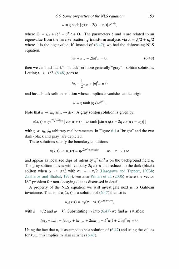
6.6 Some properties of the NLS equation 153
u = η sech[η (x + 2ξt − x0)
]e−iΘ,
where Θ = ξx + (ξ2 − η2)t + Θ0. The parameters ξ and η are related to aneigenvalue from the inverse scattering transform analysis via λ = ξ/2 + iη/2where λ is the eigenvalue. If, instead of (6.47), we had the defocusing NLSequation,
iut + uxx − 2|u|2u = 0, (6.48)
then we can find “dark” – “black” or more generally “gray” – soliton solutions.Letting t → −t/2, (6.48) goes to
iut − 12
uxx + |u|2u = 0
and has a black soliton solution whose amplitude vanishes at the origin
u = η tanh (ηx) eiη2t.
Note that u→ ±η as x→ ±∞. A gray soliton solution is given by
u(x, t) = ηe2iη2t+iψ0[
cosα + i sinα tanh[sinα η(x − 2η cosα t − x0)
] ]with η, α, x0, ψ0 arbitrary real parameters. In Figure 6.1 a “bright” and the twodark (black and gray) are depicted.
These solutions satisfy the boundary conditions
u(x, t)→ u±(t) = ηe2iη2t+iψ0±iα as x→ ±∞and appear as localized dips of intensity η2 sin2 α on the background field η.The gray soliton moves with velocity 2η cosα and reduces to the dark (black)soliton when α → π/2 with ψ0 = −π/2 (Hasegawa and Tappert, 1973b;Zakharov and Shabat, 1973); see also Prinari et al. (2006) where the vectorIST problem for non-decaying data is discussed in detail.
A property of the NLS equation we will investigate next is its Galileaninvariance. That is, if u1(x, t) is a solution of (6.47) then so is
u2(x, t) = u1(x − vt, t)ei(kx−ωt),
with k = v/2 and ω = k2. Substituting u2 into (6.47) we find u1 satisfies:
iu1,t + ωu1 − ivu1,x + (u1,xx + 2iku1,x − k2u1) + 2|u1|2u1 = 0.
Using the fact that u1 is assumed to be a solution of (6.47) and using the valuesfor k, ω, this implies u2 also satisfies (6.47).
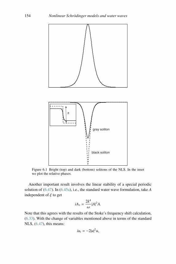
154 Nonlinear Schrodinger models and water waves
π
black soliton
gray soliton
Figure 6.1 Bright (top) and dark (bottom) solitons of the NLS. In the insetwe plot the relative phases.
Another important result involves the linear stability of a special periodicsolution of (6.47). In (6.45a), i.e., the standard water wave formulation, take Aindependent of ξ to get
iAτ =2k4
ω|A|2A.
Note that this agrees with the results of the Stoke’s frequency shift calculation,(6.33). With the change of variables mentioned above in terms of the standardNLS, (6.47), this means:
iut = −2|u|2u,
6.6 Some properties of the NLS equation 155
which has the plane wave solution u = ae2ia2t, a = u(0); for convenience takea real. We now perturb this solution: u = ae2ia2t(1 + ε(x, t)), where |ε| � 1.Substituting this into (6.47) and linearizing (i.e., assuming |ε| � 1) we find,
iεt + εxx + 2a2 (ε + ε∗) = 0.
We will consider the linearized problem on the periodic spatial domain 0 <
x < L. Thus, ε(x, t) has the Fourier expansion
ε(x, t) =∞∑−∞
εn(t)eiμn x,
where μn = 2πn/L. Note that ε−n(t) is not the complex conjugate of εn(t), sinceε is not necessarily real. Since the PDE is linear, it is sufficient to considerε = εn(t)eiμn x + ε−n(t)e−iμn x. Thus, with ε ′n ≡ ∂εn/∂t,
i(ε ′neiμn x + ε ′−ne−iμn x
)− μ2
n
(εneiμn x + ε−ne−iμn x
)+ 2a2
(εneiμn x + ε−ne−iμn x + ε ∗ne−iμn x + ε ∗−neiμn x
)= 0.
Setting to zero the coefficients of eiμn x and e−iμn x, we find, respectively,
iε ′n − μ2nεn + 2a2 (εn + ε
∗−n)= 0
iε ′−n − μ2nε−n + 2a2 (ε−n + ε
∗n)= 0.
Taking the conjugate of the last equation and multiplying it by −1, we have thesystem
i∂
∂t
(εn
ε ∗−n
)+
(2a2 − μ2
n 2a2
−2a2 −2a2 + μ2n
) (εn
ε ∗−n
)= 0,
to solve. Assuming a solution of the form(εn
ε ∗−n
)=
(α
β
)eiσnt,
we find
det
(2a2 − μ2
n − σn 2a2
−2a2 −2a2 + μ2n − σn
)= 0
must be true, hence with μ2n = (2nπ/L)2
σ2n =
(2πnL
)2 ⎡⎢⎢⎢⎢⎢⎣(2πnL
)2− 4a2
⎤⎥⎥⎥⎥⎥⎦ .
156 Nonlinear Schrodinger models and water waves
Thus, whenaLπ> n
the system is unstable, since σ2n < 0 leads to exponential growth. Note that
there are only a finite number of unstable modes. In the context of water waves,we have deduced the famous result by Benjamin and Feir (1967) that the Stokeswater wave is unstable. Later, Benney and Roskes (1969) (BR) showed thatall periodic wave solutions of the slowly varying envelope water wave equa-tions in 2 + 1 dimensions are unstable. The BR equations are also discussedbelow. We also remark that Zakharov and Rubenchik (1974) showed that soli-tons are unstable to weak transverse modulations, i.e., one-dimensional solitonsolutions of
iut + uxx + ε2uyy + 2|u|2u = 0
are unstable. (See Ablowitz and Segur, 1979 for further discussion.)
6.7 Higher-order corrections to the NLS equation
As mentioned earlier, the nonlinear Schrodinger equation was first derived in1968 in deep water with surface tension by Zakharov (1968) and its finite depthanalog in 1969 by Benney and Roskes (1969). It took some ten years until in1979 Dysthe (1979) derived, in the context of deep-water waves, the next-order correction to the NLS equation. We simply quote the (1+1)-dimensionalresult:
2iω(AT + vgAX
)− ε(v2
gAXX + 4k2|A|2A)
= ε2
(iω2
8k3AXXX + 2ik3A2A∗X− 12ik3|A|2AX + 2ωkφXA
). (6.49)
The mean term φX is unique to deep-water waves and arises from the quadraticnonlinearity in the water wave equations. The mean field satisfies
φXX + φZZ = 0, −∞ < z < 0,
with φZ → 0 as z→ −∞ and
φZ =2ωk
g∂
∂X|A|2, z = 0.
Non-dimensionalizing (6.49) by setting T ′ = ωT , X′ = kX, Z′ = kZ, η′ = kη,φ′= (2k2/ω)φ, u =
(2√
2k2/ω)
A, τ = −εT ′/8, and ξ = X′ − T ′/2, we get
6.7 Higher-order corrections to the NLS equation 157
iuτ + uξξ + 2|u|2u + ε( i2
uξξξ − 6i|u|2uξ + iu2u∗ξ + 2uH[|u|2]ξ)= 0, (6.50)
where
H[ f ] =1π−∫
f (u)u − x
du
is the so-called Hilbert transform. (The integral is understood in the principle-value sense.) Ablowitz, Hammack, Henderson, and Schober (Ablowitz et al.,2000a, 2001) showed that periodic solutions of (6.50) can actually be chaotic.Experimentally and analytically, a class of periodic solutions is found not tobe “repeatable”, while soliton solutions are repeatable.
To go from the term including φx in (6.49) to the Hilbert transform requiressome attention. The velocity potential satisfies Laplace’s equation:
φxx + φzz = 0.
In the Fourier domain, with φ =∫
φe−iξx dx, we find
φzz − ξ2φ = 0.
Using the boundary condition φz → 0 as z→ −∞, we get
φ(ξ, z) = C(ξ)e|ξ|z,
where C is to be determined. The factor C is fixed by the boundary condition
φz =2ωk
g∂
∂x|A|2,
on z = 0. Hence
C(ξ) =2iωk
gξ
|ξ|F (|A|2) =2iωk
gsgn(ξ)|F (|A|2)
where F represents the Fourier transform. Using a well-known result fromFourier transforms, F −1[sgnξF(ξ)] = H[ f (x)], where f is the inverse Fouriertransform of F and H[·] is the Hilbert transform (Ablowitz and Fokas, 2003)and noting thatH
[eiξx]= i sgn(ξ)eiξx, we have
φ =2ωk
gH[|A|2]
φx =2ωk
g∂
∂xH[|A|2].
158 Nonlinear Schrodinger models and water waves
6.8 Multidimensional water waves
For multidimensional water waves in finite depth with surface tension, thevelocity potential has the form
φ = ε(φ(X,Y,T ) +cosh(k(z + h))
cosh(kh)(A(X,Y,T )ei(kx−ωt) + c.c.)) + O(ε2),
where X = εx, Y = εy, T = εt and φ, A satisfy coupled nonlinear wave equa-tions. Benney and Roskes (1969) derived this system without surface tension.It was subsequently rederived by Davey and Stewartson (1974) who put thesystem in a simpler form. Later, Djordjevic and Redekopp (1977) includedsurface tension.
After non-dimensionalization and rescaling, the equations can be put intothe following form; we call it a Benney–Roskes (BR) system:
iAt + σ1Axx + Ayy = σ2|A|2A + AΦx
aΦxx + Φyy = −b(|A|2)x
σ1 = ±1, σ2 = ±1.
(6.51)
The parameters σ1, σ2, a, and b are dimensionless and depend on the dimen-sionless fluid depth and surface tension. Here we have presented it in arescaled, normalized form that helps in analyzing its behavior for differentchoices of σ1 and σ2. The quantity A is related to the slowly varying envelopeof the first harmonic of the potential velocity field andΦ is related to the slowlyvarying mean potential velocity field.
A special solution to (6.51) is the following self-similar solution
A =Λ
texp i
(σ1x2 + y2
4t+ σ2
Λ2
t+ B(t) + φ0
)Φ = −B′(t)x +C(t)y + D(t).
This is an analog of the similarity solution of the one-dimensional nonlinearSchrodinger (NLS) equation
iAt + Axx + σ|A|2A = 0
A =Λ
t1/2exp i
(x2
4t+ σΛ2 log(t) + φ0
).
Since the above similarity solution of NLS approximates the long-time solu-
tion of NLS without solitons in the region
∣∣∣∣∣∣ x√t
∣∣∣∣∣∣ ≤ O(1), it can be expected
that the similarity solution of the BR system is a candidate to approximatelong-time “radiative” solutions.
6.8 Multidimensional water waves 159
From the water wave equations in the limit kh→ 0 (the shallow-water limit)with suitable rescaling, cf. Ablowitz and Segur (1979), the BR system (6.51)reduces to
iAt − γAxx + Ayy = A(γ|A|2 + Φx)
γΦxx + Φyy = −2(|A|2)x, γ = sgn(
13 − T
)= ±1.
(6.52)
This is the so-called Davey–Stewartson (DS) equation. As we have mentioned,it describes multidimensional water waves in the slowly varying envelopeapproximation, with surface tension included, in the shallow-water limit. Here
the normalized surface tension is defined as T =T0
ρgh2, T0 being the surface
tension coefficient. This system, (6.52), is integrable (Ablowitz and Clarkson,1991) whereas the multidimensional deep-water limit
iAt + ∇2A + |A|2A = 0
is apparently not integrable. The concept of integrability is discussed in moredetail in Chapters 8 and 9 (cf. also Ablowitz and Clarkson 1991).
The DS equation (6.52) can be generalized by making the followingsubstitutions
φ = Φx, r = −σq∗ = −σA∗, σ = ±1
and we write
iqt − γqxx + qyy = q(φ − qr)
φxx + γφyy = 2(qr)xx.(6.53)
With q = A, γ = −1, and σ = 1, we get shallow-water waves with“large” surface tension, equation (6.52). It turns out that the generalized DSequation (GDS), (6.53), admits “localized” boundary induced pulse solutionswhen γ= 1 (Ablowitz and Clarkson, 1991) and weakly decaying “lump”-typesolutions when γ = −1 (Villarroel and Ablowitz, 2003).
6.8.1 Special solutions of the Davey–Stewartson equations
Consider the case where γ = −1 with σ = 1. Then the DS system (6.53)becomes
2iqt + qxx + qyy = 2(φ − qr)q
φxx − φyy = 2(qr)xx.(6.54)
We call this the DSI system. Note that the DSI system admits an interest-ing class of solutions, cf. Fokas and Santini (1989, 1990) and Ablowitz et al.
160 Nonlinear Schrodinger models and water waves
(2001a). In order to write down the pulse solution (also called a “dromion”),we will make a convenient rescaling and change of variable as follows:
Q = φ − qr.
Then the second equation in GDS system (6.54) becomes
Qxx − Qyy = (qr)xx + (qr)yy. (6.55)
Now we make the change of variable
ξ =x + y√
2, η =
x − y√2
∂x =1√2
(∂ξ + ∂η), ∂y =1√2
(∂ξ − ∂η)
to transform (6.55) to
2Qξη = (qr)ξξ + (qr)ηη. (6.56)
Finally, making the substitution
Q = −(U1 + U2),
and integrating with respect to ξ and η separates (6.56) into
U1 = u1(η) − 12
∫ ξ
−∞(qr)η dξ′, U2 = u2(ξ) − 1
2
∫ η
−∞(qr)ξ dη.
These two equations along with the transformed second equation in (6.54),
2iqt + qξξ + qηη + 2(U1 + U2)q = 0,
give rise to the following “dromion” solution
u1(η) = 2λ2R sech2(λR(η − η0)), η = η − 2λI t
u2(ξ) = 2μ2R sech2(μR(ξ − ξ0)), ξ = ξ − 2μI t
q =ρ√λRμReiθ
cosh(μR(ξ − ξ0)) cosh(λR(η − η0)) + (|ρ|/2)2e(λR(η−η0))eμR(ξ−ξ0)
θ = −(μI ξ + λI η) + (|μ|2 + |λ|2)t2− θ0
λ = λR + iλI , μ = μR + iμI constants.
where λR > 0, μR > 0, λ, μ, ρ are complex constants and ξ0, η0 arereal constants. See Figure 6.2 where a typical dromion is depicted (withλR = 1, μR = 1, λI = 0, μI = 0, ρ = 1).
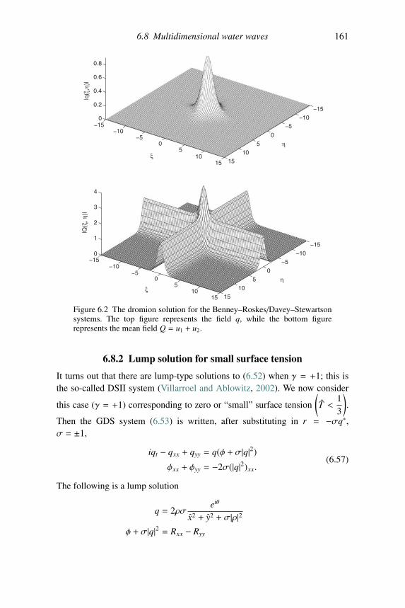
6.8 Multidimensional water waves 161
−15
−10
−5
0
5
10
15
−15−10
−50
510
15
0
1
2
3
4
η
ξ
|Q(ξ
, η)|
−15−10
−5
0
510
15
−15−10
−50
510
15
0
0.2
0.4
0.6
0.8
η
ξ
|q(ξ
,η)|
Figure 6.2 The dromion solution for the Benney–Roskes/Davey–Stewartsonsystems. The top figure represents the field q, while the bottom figurerepresents the mean field Q = u1 + u2.
6.8.2 Lump solution for small surface tension
It turns out that there are lump-type solutions to (6.52) when γ = +1; this isthe so-called DSII system (Villarroel and Ablowitz, 2002). We now consider
this case (γ = +1) corresponding to zero or “small” surface tension
(T <
13
).
Then the GDS system (6.53) is written, after substituting in r = −σq∗,σ = ±1,
iqt − qxx + qyy = q(φ + σ|q|2)
φxx + φyy = −2σ(|q|2)xx.(6.57)
The following is a lump solution
q = 2ρσeiθ
x2 + y2 + σ|ρ|2φ + σ|q|2 = Rxx − Ryy
162 Nonlinear Schrodinger models and water waves
R = log(x2 + y2 + σ|ρ|2) (6.58)
θ = ax − by + (b2 − a2)t − θ0
x = x + at − x0, y = y + bt − y0
k = 12 (a + ib) constant.
This solution is non-singular when σ = 1, but for σ = −1, the abovesolution is singular. Alternatively we have the interesting case of the darklump-type envelope hole solution (Satsuma and Ablowitz, 1979) whenσ=− 1.The case σ = 1 occurs in water waves; i.e., in this case, (6.57) can betransformed to the reduced water wave equation (6.52). But it has beenshown that the lump solution (6.58) is unstable (Pelinovsky and Sulem,2000).
We also note that Ablowitz et al. (1990) discussed the derivation of theintegrable equations (6.54) and (6.57) from the KPI and KPII equations,respectively.
6.8.3 Multidimensional problems and wave collapse
As mentioned earlier, in 1969 Benny and Roskes derived a (2+1)-dimensionalNLS-type equation for water waves (Benney and Roskes, 1969). In 1977Djordjevic and Redekopp extended their results by including surface tensioneffects (Djordjevic and Redekopp, 1977). To get these equations the velocitypotential expansion takes the form:
φ = ε(φ(X,Y,T ) +cosh [k(h + z)]
cosh kh
(A(X,Y,T )eiθ + c.c.
)) + O(ε2),
θ = kx − ωt, X = εx,Y = εy,T = εt
ω2 = gκ tanh(κh)(1 + T ),
κ2 = k2 + l2,
T =k2Tρg
.
In terms of the redefined functions: A = Ak2√gk
, Φ =k2√gkφ, and variables:
ξ = k(X − ω′T ), τ =√
gkε2t, η = εkY , we have that A, Φ satisfy the followingcoupled system
iAτ + λAξξ + μAηη = χ|A|2A + χ1AΦξ (6.59)
αΦξξ + Φηη = −β(|A|2)ξ. (6.60)
6.8 Multidimensional water waves 163
The parameters λ, μ, χ, χ1, α, and β depend on ω, k, T , and gh (see Ablowitzand Segur, 1979, 1981). As h→ ∞, (6.59) reduces to an NLS equation
iAτ + λ∞Aξξ + μ∞Aηη − χ∞|A|2A = 0,
where
λ∞ = −ω0
8ω
⎛⎜⎜⎜⎜⎝1 − 6T − 3T 2
1 + T
⎞⎟⎟⎟⎟⎠μ∞ =
ω0
4ω
(1 + 3T
)χ∞ =
ω0
4ω
⎡⎢⎢⎢⎢⎢⎢⎣ 8 + T + 2T 2(1 − 2T
) (1 + T
) ⎤⎥⎥⎥⎥⎥⎥⎦ω2
0 = gκ,
with λ∞ > 0, μ∞ > 0 and −ξ∞ > 0 for T large enough. This equa-tion has solutions that blow-up in finite time (Ablowitz and Segur, 1979).When T = 1/2, the expansion breaks down due to second harmonic resonance:ω2(2k) = [2ω(k)]2. However, when T = 0, i.e., when there is no surfacetension, some of the coefficients in the above equation change sign and wehave
(ω0ω> 0): λ∞ < 0, μ∞ > 0 and χ∞ > 0. To date no blow-up has been
found for the above NLS equation with the latter choices of signs.
Blow-upOne can verify that
iAt + ΔA + |A|2A = 0, x ∈ R2
has the conserved quantities
P(t) =∫|A|2 dx,
M(t) =∫
A∇A dx
H(t) =∫|∇A|2 − 1
2|A|4 dx,
i.e., mass (power), momentum, and energy (Hamiltonian) are conserved.Define
V(t) =∫|r|2|A|2 dx,
164 Nonlinear Schrodinger models and water waves
where |r|2 = x2 + y2. Then one can show that in two dimensions (Vlasov et al.,1970),
d2Vdt2= 8H.
This is often called the virial theorem. Integrating this equation, we get
V(t) = 4Ht2 + c1t + c0.
If the initial conditions are such that H < 0, then there exists a time t∗ when
limt→t∗
V(t) = 0
and for t > t∗, V(t) < 0. However, V is a positive quantity. Thus a singularityin the solution has occurred in finite time t = t∗. Combining this result with theconservation of mass and a bit more analysis, one can show that in fact∫
|∇A|2 dx
becomes infinite as t → t∗, which in turn implies that A also becomes infi-nite as t → t∗. For an extensive discussion of the NLS equation in one andmultidimensions, see Sulem and Sulem (1999).
The more general equation
iψt + Δdψ + |ψ|2σψ = 0, x ∈ Rd, (6.61)
where Δd is the d-dimensional Laplacian, has also been studied. There are threecases:• “supercritical”: σd > 2 blow-up occurs;• “critical”: σd = 2 blow-up can occur; collapse can be arrested with small
perturbations;• “subcritical”: σd < 2 global solutions exist.A special solution to (6.61) can be found by assuming a solution of the formψ = f (r)eiλt. In two dimensions, we find the nonlinear eigenvalue problem
1r∂
∂r
(r∂ f∂r
)+ f 3 − λ f = 0,
certain solutions to which are the so-called Townes modes. Asymptotically,f ∼ e−r/
√r, 1 � r (Fibich and Papanicolaou, 1999). Weinstein (1983) showed
that there is a critical energy (found from the Townes mode with the smallestenergy),
Ec =
∫|u|2dxdy = 2π
∫ ∞
0r f 2(r) dr � 2π(1.86) � 11.68.
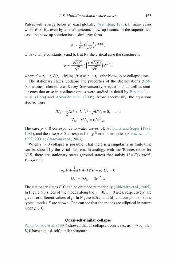
6.8 Multidimensional water waves 165
Pulses with energy below Ec exist globally (Weinstein, 1983). In many caseswhen E > Ec, even by a small amount, blow-up occurs. In the supercriticalcase, the blow-up solution has a similarity form
ψ ∼ 1t′α
f( rt′β)
eiλ ln t′ ,
with suitable constants α and β. But for the critical case the structure is
ψ ∼√
L(t′)√t′
f
(r√
L(t′)√t′
)eiφ(t′),
where t′ = tc − t, L(t) ∼ ln(ln(1/t′)) as t → tc is the blow-up or collapse time.The stationary states, collapse and properties of the BR equations (6.59)
(sometimes referred to as Davey–Stewartson-type equations) as well as simi-lar ones that arise in nonlinear optics were studied in detail by Papanicolaouet al. (1994) and Ablowitz et al. (2005). More specifically, the equationsstudied were
iUz +12ΔU + |U |2U − ρUVx = 0, and
Vxx + νVyy = (|U |2)x.
The case ρ < 0 corresponds to water waves, cf. Ablowitz and Segur (1979,1981), and the case ρ > 0 corresponds to χ(2) nonlinear optics (Ablowitz et al.,1997, 2001a; Crasovan et al., 2003).
When ν > 0 collapse is possible. That there is a singularity in finite timecan be shown by the virial theorem. In analogy with the Townes mode forNLS, there are stationary states (ground states) that satisfy U = F(x, y)eiμz,V =G(x, y)
−μF +12ΔF + |F|2F − ρFGx = 0
Gxx + νGyy = (|F|2)x.
The stationary states F,G can be obtained numerically (Ablowitz et al., 2005).In Figure 6.3 slices of the modes along the y = 0, x = 0 axes, respectively, aregiven for different values of ρ. In Figure 6.3(c) and (d) contour plots of sometypical modes F are shown. One can see that the modes are elliptical in naturewhen ρ � 0.
Quasi-self-similar collapsePapanicolaou et al. (1994) showed that as collapse occurs, i.e., as z→ zc, thenU,V have a quasi-self-similar structure:

166 Nonlinear Schrodinger models and water waves
−5 50
3
x|F
(x,y
= 0
)|
(a)
−5 50
3
y
|F(x
= 0
,y)|
(b)
x
y
(c)
−3 3−3
3
x
y
(d)
−3 3−3
3
Figure 6.3 F(x, y); ν = 0.5; top (a), (b): “slices”; bottom: contour plots; (c)ρ = −1, (d)ρ = 1.
−6 60
3
x
z = 0 L = 0.96
−6 60
3
x
z = 0.5 L = 0.56
−6 60
3
x
z = 0.94 L = 0.22
F(x,0)
L|u(Lx,0)|
−6 60
3
y−6 60
3
y−6 60
3
y
F(0,y)
L|u(0,Ly)|
Figure 6.4 Wave collapse to the stationary state as z→ zc.
U ∼ 1L(z)
F
(x
L(z),
yL(z)
), V ∼ 1
L(z)G
(x
L(z),
yL(z)
)where L → 0. Further, one finds from direct simulation (Ablowitzet al., 2005) that the stationary modes are good approximations ofcollapse profiles. By taking typical initial conditions (of Gaussiantype) that collapse, we find that the pulse structure is well approx-imated by the stationary modes in the neighborhood of the collapsepoint, where L(z)= F(0, 0)/U(0, 0, z)→ 0. In Figure 6.4 we compareL(z)|U(Lx, Ly)| with F(x, y) where L(z)= F(0, 0)/U(0, 0, z). As collapseoccurs, L(z)→ 0 for typical values (ν, ρ) = (0.5, 1). In Figure 6.4 we pro-vide snapshots of the solution compared to the stationary state F as the wave
Exercises 167
collapse begins to occur. Along the y = 0 axis (top) and the x = 0 axis (bottom)at the edges of the solution, radiation is seen. But the behavior at the center ofthe wave indicates that collapse is well approximated by the stationary state.
Finally, we mention that a similar, but more complicated blow-up or wavecollapse phenomenon occurs for the generalized KdV equation
ut + upux + uxxx = 0
when p ≥ 4 (Ablowitz and Segur, 1981; Merle, 2001; Angulo et al., 2002).
Exercises
6.1 Derive the NLS equation from the following nonlinear equations.(a) utt − uxx + sinu = 0 (sine–Gordon).(b) utt − uxx + uxxxx + (uux)x = 0 (Boussinesq-type).(c) ut + u2ux + uxxx = 0 (mKdV) .
6.2 Given the equation
iut − uxxxx + |u|2(n+1)u = 0
with n ≥ 1 an integer, substitute the mutli-scale and quasi-monochromatic assumption:
u ∼ μe(ikx−ωt)A(ε1x, ε2t),
where μ, ε1, and ε2 are all asymptotically small parameters, into theequation. Choose a maximal balance between the small parameters tofind a nonlinear Schrodinger-type wave equation for the slowly varyingenvelope A.
6.3 From the water wave equations with surface tension included, derive thedispersion relation
ω2 = gκ tanh(κh)(1 + T ), κ2 = k2 + l2, T =k2T0
ρg
in finite depth water waves with surface tension, where T0 is the surfacetension coefficient.
6.4 Beginning with the KP equation
∂x(ut + 6uux + uxxx) + 3σuyy = 0, σ = ±1
derive the integrable Davey–Stewartson equation by employing theslowly varying quasi-monochromatic wave expansion. Hint: seeAblowitz et al. (1990).
168 Nonlinear Schrodinger models and water waves
6.5 Suppose we are given a “modified KP” equation
∂x
(ut +
3n + 1
(u2(n+1))x + uxxx
)+ 3σuyy = 0, σ = ±1
where n ≥ 1, an integer. Following a similar analysis as in the previousexercise, derive a “modified” Davey–Stewartson equation by employingthe slowly varying quasi-monochromatic wave expansion.
6.6 Suppose we are given the “damped NLS” equation
iut + uxx + 2|u|2u = −iγu
where 0 < γ � 1. Use the integral relation involving mass (power)∫ |u|2dx to derive an approximate evolution equation for the slowlyvarying soliton amplitude η where the unperturbed soliton is given by
u = ηsech[η (x − x0)
]eiη2t+iθ0 .
Hint: see Ablowitz and Segur (1981). Various perturbation problemsinvolving related NLS-type equations are also discussed in Chapter 10.
6.7 Discuss the stability associated with the special solution
u = aei(kx−(k2−2σ|a|2)t)
where k, σ are constant, associated with the NLS equation
iut + uxx + 2σ|u|2u = 0
on the infinite interval.6.8 Given the two-dimensional NLS equation
iAt + ΔA + |A|2A = 0, x ∈ R2
and associated “Townes” mode A = f (r)eiλt, where r2 = x2 + y2, showthat the “virial” equation reduces to
d2Vdt2= 0
where V(t) =∫
(x2 + y2)|A|2 dx. Hint: see the appendix in Ablowitz et al.(2005).
7Nonlinear Schrodinger models in nonlinear optics
An important and rich area of application of nonlinear wave propagation is thefield of nonlinear optics. Asymptotic methods play an important role in thisfield. For example, since the scales are so disparate in Maxwell’s equations,long-distance transmission in fiber optic communications depends critically onasymptotic models. Hence the nonlinear Schrodinger (NLS) equation is cen-tral for understanding phenomena and detailed descriptions of the dynamics.In this chapter we will outline the derivation of the NLS equation for electro-magnetic wave propagation in bulk optical media. We also briefly discuss howthe NLS equation arises as a model of spin waves in magnetic media.
7.1 Maxwell equations
We begin by considering Maxwell’s equations for electromagnetic waves withno source charges or currents, cf. Landau et al. (1984) and Jackson (1998)
∇ × H =∂D∂t
(7.1a)
∇ × E = −∂B∂t
(7.1b)
∇ · D = 0 (7.1c)
∇ · B = 0 (7.1d)
where H is the magnetic field, E is the electromagnetic field, D is theelectromagnetic displacement and B is the magnetic induction.
We first consider non-magnetic media so there is no magnetization term inB. The magnetic induction B and magnetic field H are then related by
B = μ0H. (7.2)
169
170 Nonlinear Schrodinger models in nonlinear optics
The constant μ0 is the magnetic permeability of free space. We allow forinduced polarization of the media giving rise to the following relation
D = ε0(E + P), (7.3)
where ε0 is the electric permittivity of free space, a constant. When we applyan electric field E to an ideal dielectric material a response of the material canoccur and the material is said to become polarized. Typically in these materialsthe electrons are tightly bound to the nucleus and a displacement of theseelectrons occurs. The macroscopic effect (summing over all displacements)yields the induced polarization P.
Since we are working with non-magnetic media, we can reduce Maxwell’sequations to those involving only the electromagnetic field E and the polar-ization P. To that end, we take the curl of (7.1b) and use (7.2) and (7.1a)to find
∇ × (∇ × E) = − ∂∂t
(∇ × B)
= −μ0∂
∂t(∇ × H)
= −μ0∂2
∂t2D.
The vector identity
∇ × (∇ × E) = ∇(∇ · E) − ∇2E, (7.4)
is useful here. With this, along with relation (7.3), we find the followingequations for the electromagnetic field
∇2E − ∇(∇ · E) =1c2
∂2
∂t2(E + P(E))
∇ · (E + P(E)) = 0,(7.5)
where the constant c2 =1μ0ε0
is the square of the speed of light in a vacuum.
Notice that we have made explicit the connection between the polarization Pand the electromagnetic field E.
Before we investigate polarizable, non-magnetic media in detail, let us alsowrite down the dual equation for magnetic media without polarization (P = 0)satisfying
B = μ0(H + M(H)) (7.6)
where M is called the magnetization. We see that the magnetization vectorM plays a similar role to that of the polarization P, i.e., we are assuming
7.2 Polarization 171
that M = M(H). Namely, we assume that the magnetization is related tothe magnetic field. The magnetization can be permanent for ferromagneticmaterials (permanent magnets such as iron). Taking the curl of (7.1a) thenfor non-polarized media using D = ε0E gives
∇ × (∇ × H) =∂
∂t(∇ × D)
= ε0∂
∂t(∇ × E)
= −ε0∂2
∂t2B.
Using (7.4) and (7.6) gives
∇2H − ∇(∇ · H) =1c2
∂2
∂t2(H + M(H))
∇ · (H + M(H)) = 0.
Later, in Section 7.4 we will discuss one way M can be coupled to H.
7.2 Polarization
In homogeneous, non-magnetic media, matter responds to intense electromag-netic fields in a nonlinear manner. In order to model this, we use a well-knownrelationship between the polarization vector P and the electromagnetic field Ethat is a good approximation to a wide class of physically relevant media:
P(E) =∫
χ(1) ∗ E +∫
χ(2) ∗ EE +∫
χ(3) ∗ EEE. (7.7)
The above equation involves tensors, so the operation ∗ is a special type ofconvolution that will be defined below.
For notational purposes, we will write the polarization vector as follows:
P =
⎛⎜⎜⎜⎜⎜⎜⎜⎜⎜⎝Px
Py
Pz
⎞⎟⎟⎟⎟⎟⎟⎟⎟⎟⎠ ≡⎛⎜⎜⎜⎜⎜⎜⎜⎜⎜⎝
P1
P2
P3
⎞⎟⎟⎟⎟⎟⎟⎟⎟⎟⎠ .Notice that we can break up (7.7) into a linear and nonlinear part
P = PL + PNL.
In glass, and hence fiber optics, the quadratic term χ(2) is zero. This is cubicallynonlinear and is a so-called “centro-symmetric material”, cf. Agrawal (2001),Boyd (2003) and also Ablowitz et al. (1997, 2001a) and included references
172 Nonlinear Schrodinger models in nonlinear optics
for more information. We write the linear and nonlinear components of thepolarization vector, and explicitly define the convolution mentioned above, asfollows:
PL,i = (χ(1) ∗ E)i =
3∑j=1
∫ ∞
−∞χ(1)
i j (t − τ)E j(τ) dτ (7.8)
PNL,i =∑j,k,l
∫ ∞
−∞χ(3)
i jkl(t − τ1, t−τ2, t − τ3)E j(τ1)Ek(τ2)El(τ3) dτ1dτ2dτ3. (7.9)
In (7.9), the sums are over the indices {1, 2, 3} and the integration is overall of R3. The matrix χ(1) is called the linear susceptibility and the tensorχ(3) is the third-order susceptibility. If the material is “isotropic”, χ(1)
i j = 0,i� j (exhibiting properties with the same values when measured along axes inall directions), then the matrix χ(1) is diagonal. We will also usually identifysubscripts i = 1, 2, 3 as i = x, y, z. In cubically nonlinear or “Kerr” materials(such as glass), it turns out that the only important terms in the χ(3) tensorcorrespond to χ(3)
xxxx, which is equal to χ(3)yyyy and χ(3)
zzzz.From now on, we will suppress the superscript in χ when context makes
the choice clear. For example χ(1)xx = χxx and χ(3)
xxxx = χxxxx follow due to thenumber of entries in the subscript.
We can now pose the problem of determining the electromagnetic field E inKerr media as solving (7.5) subject to (7.8) and (7.9). Consider the asymptoticexpansion
E = εE(1) + ε2E(2) + ε3E(3) + · · · , |ε| � 1. (7.10)
Then, to leading order, we assume that the electromagnetic field is initiallypolarized along the x-axis; it propagates along the z-axis, and for simplicitywe assume no transverse y variations. So
E(1) =
⎛⎜⎜⎜⎜⎜⎜⎜⎜⎜⎝E(1)
x
00
⎞⎟⎟⎟⎟⎟⎟⎟⎟⎟⎠ , E(1)x = A(X,Z,T )eiθ + c.c., (7.11)
where θ = kz − ωt and the amplitude A is assumed to be slowly varying in thex, z, and t directions:
X = εx, Z = εz, T = εt.
In order to simplify the calculations, we assume E and hence A are independentof y (i.e., Y = εy). Derivatives are replaced as follows
7.2 Polarization 173
∂x = ε∂X
∂t = −ω∂θ + ε∂T
∂z = k∂θ + ε∂Z .
(7.12)
Substituting in the asymptotic expansion for E we note the importantsimplification that the assumption of slow variation has on the polarization P:
PL,x =
3∑j=1
∫ ∞
−∞χ(1)
x j (t − τ)E j(τ) dτ
= ε
∫ ∞
−∞χxx(t − τ)
(A(X,Z,T )ei(kz−ωτ) + c.c.
)dτ + O(ε2)
= ε
∫ ∞
−∞χxx(t − τ)eiω(t−τ)
(A(X,Z,T )ei(kz−ωt) + c.c.
)dτ + O(ε2).
Now make the substitution t − τ = u to get
PL,x = ε
∫ ∞
−∞χxx(u)eiωu
(A(X,Z, εt − εu)ei(kz−ωt) + c.c.
)du + O(ε2).
We expand the slowly varying amplitude A around the point εt
PL,x =ε
∫ ∞
−∞du χxx(u)eiωu×[(
1 − εu∂
∂T+
(εu)2
2∂2
∂T 2+ · · ·
)A(X,Z,T )ei(kz−ωt) + c.c.
]+ O(ε2).
Recall that the Fourier transform of χxx, written as χxx, and its derivatives are
χxx(ω) =∫ ∞
−∞χxx(u)eiωu du
χ′xx(ω) =∫ ∞
−∞iuχxx(u)eiωu du
χ′′xx(ω) =∫ ∞
−∞−u2χxx(u)eiωu du.
Then we can write the linear part of the polarization as
PL,x = ε
(χxx(ω) + χ′xx(ω)iε∂T − χ′′xx(ω)
(ε∂T )2
2+ · · ·
)(Aeiθ + c.c.) + O(ε2)
= εχxx(ω + iε∂T )(Aeiθ + c.c.) + O(ε2).
174 Nonlinear Schrodinger models in nonlinear optics
The last line is in a convenient notation where the term χxx(ω + iε∂T ) is anoperator that we can expand around ω to get the previous line.
In the nonlinear polarization equation (7.9), there will be interactions dueto the leading-order mode Aeiθ, for example, the nonlinear term includes E3
x ,which leads to terms such as A3e3iθ. Then we denote the corresponding linearpolarization term (containing interaction terms) as
PinteractionsL,x = χxx(ωm + iε∂T )(Bmeimθ + c.c.),
where ωm = mω and Bm contains the nonlinear terms generated by theinteraction (e.g. B3 = A3).
Similarly there are nonlinear polarization terms. For example, a typical termin the nonlinear polarization is
PNL,x = ε3χxxxx(ωm + iε∂T1 , ωn + iε∂T2 , ωl + iε∂T3 )
× Bm(T1)Bn(T2)Bl(T3)∣∣∣T1=T2=T3=T ei(m+n+l)θ + c.c.
(7.13)
All other terms are of smaller order O(ε4).
7.3 Derivation of the NLS equation
So far, we have derived expressions for the polarization with a cubic nonlin-earity (third-order susceptibility). Now we will use (7.5) to derive the NLSequation. This will give the leading-order equation for the slowly varyingamplitude of the x-component of the electromagnetic field Ex.
We begin the derivation of the NLS equation by showing that Ez � Ex.Recall (7.1c) with (7.3),
∇ · (E + P) = 0.
Since there is no y dependence, we get
∂x(Ex + Px) + ∂z(Ez + Pz) = 0. (7.14)
We assume
Ex = εA(X,Z,T )eiθ + c.c. + O(ε2)
Ez = εAz(X,Z,T )eiθ + c.c. + O(ε2),(7.15)
where as before c.c. denotes the complex conjugate of the preceding term. Afurther note on notation. Because the x-component of the electromagnetic fieldEx appears so often, we label its slowly varying amplitude with A, whereas
7.3 Derivation of the NLS equation 175
for the z-component of the E-field, Ez, we label the slowly varying amplitudewith Az (note: Az does not mean derivative with respect to z).
Substituting the derivatives (7.12) into (7.14) we find
(k∂θ + ε∂Z)(Ez + Pz) = −ε∂X(Ex + Px),
which, when we use the ansatz (7.15), yields
ε(k∂θ + ε∂Z)(Aze
iθ + c.c. + χzz(ω + iε∂T )(Azeiθ + c.c.)
)= −ε∂X
(εAeiθ + c.c. + χxx(ω + iε∂T )(εAeiθ + c.c.)
)+ · · · .
The leading-order equation is
εikAz(1 + χzz(ω)) = −ε2 ∂A∂X
(1 + χxx(ω)) implying
Az = −ε 1 + χxx(ω)ik(1 + χzz(ω))
∂A∂X
=−εik∂A∂X= AX , if χxx = χzz.
Assuming ∂A/∂X is O(1), this implies Az = O(ε), which implies Ez = O(ε2).While we used the divergence equation in (7.5) with (7.3) to calculate thisrelationship, we could have proved the same result with the z-component ofthe dynamic equation in (7.5). We also claim that from the dynamic equationof motion in (7.5), if we had studied the y-component, then it would havefollowed that Ey = O(ε3). Also, PNL,z = O(ε4), which is obtained from thesymmetry of the third-order susceptibility tensor χ(3) since χzxxx = 0, etc. (e.g.,for glass).
Now we will use the dynamic equation in (7.5) to investigate the behavior ofthe x-component of the electromagnetic field via multiple scales. The dynamicequation (7.5) becomes
∇2Ex − ∂
∂x
(∂Ex
∂x+∂Ez
∂z
)=
1c2
∂2
∂t2(Ex + Px). (7.16)
The asymptotic expansions for Ex and Ez take the form
Ex = ε(Aeiθ + c.c.) + ε2E(2)x + ε
3E(3)x + · · ·
Ez = ε2(Aze
iθ + c.c.) + ε3E(2)z + · · · .
(7.17)
176 Nonlinear Schrodinger models in nonlinear optics
The polarization in the x-direction depends on the linear and nonlinear polar-ization terms, PL,x and PNL,x, but the nonlinear term comes in at O(ε3) due tothe cubic nonlinearity. Explicitly, we have
Px = ε(χxx(ω) + χ′xx(ω)iε∂T − χ′′xx(ω)2
ε2∂2T + · · · )(Aeiθ + c.c.) + PNL,x. (7.18)
Expanding the derivatives and using (7.12) in (7.16) gives((k∂θ + ε∂Z)2 + ε2∂2
X
)Ex − ε∂X
(ε∂XEx + (k∂θ + ε∂Z)Ez
)=
1c2
(−ω∂θ + ε∂T )2(Ex + PL,x + PNL,x). (7.19)
The leading-order equation is
O(ε) :
(−k2 +
(ω
c
)2)A = −
(ω
c
)2χxx(ω)A.
Since we assume A � 0 the above equation determines the dispersion relation;namely solving for k(ω) we find the dispersion relation
k2 =
(ω
c
)2(1 + χxx(ω))
k(ω) =ω
c(1 + χxx(ω))1/2
≡ ω
cn0(ω).
(7.20)
The term n0(ω) is called the linear index of refraction; if it were constant thenc/n0 would be the “effective speed of light”. The slowly varying amplitudeA(X,Z,T ) is still free and will be determined by going to higher order andremoving secular terms.
From (7.19) and the asymptotic expansions for Ex and PL,x in (7.17)and (7.18) (the nonlinear polarization term, PNL,x, does not come in until thenext order), we find
O(ε2) :
(k2 −
(ω
c
)2)∂2θE(2)
x =
[−2ik∂Z A − 2iω
c2(1 + χxx(ω))∂T A
−(ω
c
)2iχ′xx(ω)∂T A
]eiθ.
To remove secularities, we must equate the terms in brackets to zero. This canbe written as
2k∂A∂Z+
(2ωc2
(1 + χxx(ω)) +(ω
c
)2χ′xx(ω)
)∂A∂T= 0. (7.21)
7.3 Derivation of the NLS equation 177
Notice that if we differentiate the dispersion relation (7.20) with respect to ωwe find
2kk′ =2ωc2
(1 + χxx(ω)) +(ω
c
)2χ′xx(ω).
This means that we can rewrite (7.21) in terms of the group velocityvg = 1/k′(ω):
∂A∂Z+
1vg
∂A∂T= 0. (7.22)
This is a first-order equation that can be solved by the method of characteristicsgiving, to this order, A = A(T − z/vg). To obtain a more accurate equation forthe slowly varying amplitude A, we will now remove secular terms at the nextorder and obtain the nonlinear Schrodinger (NLS) equation.
As before, we perturb (7.22)
2ik
(∂A∂Z+
1vg
∂A∂T
)= ε f1 + ε
2 f2 + · · · .
Using this and (7.19) to O(ε3) and then, as we have discussed in earlierchapters, choosing f1 to remove secular terms, we find after some calculation
O(ε3) : 2ik
(∂A∂Z+ k′(ω)
∂A∂T
)+ε
[∂2
X + ∂2Z −
1c2
(1 + χxx(ω) + 2ωχ′xx(ω) +
12ω2χ′′xx(ω)
)∂2
T
]A
+3ε(ω
c
)2χxxxx(ω,ω,−ω)|A|2A = 0. (7.23)
We now see in (7.23) a term due to the nonlinear polarization PNL,x i.e.,the term with χxxxx(ω,ω,−ω). In fact, there are three choices for m, n, p inthe leading-order term for the nonlinear polarization [recall (7.13)] that giverise to the exponential eiθ (the coefficient of eiθ is the only term that inducessecularity). Namely, two of these integers are +1 and the other one is −1. Inthe bulk media we are working in, the third-order susceptibility tensor is thesame in all cases. This means
χxxxx(ω,ω,−ω) + χxxxx(ω,−ω,ω) + χxxxx(−ω,ω, ω)
= 3χxxxx(ω,ω,−ω)
≡ 3χxxxx(ω).
Let us investigate the coefficient of ATT due to the linear polarization. If wedifferentiate the dispersion relation (7.20) two times with respect to ω we getthe following result
178 Nonlinear Schrodinger models in nonlinear optics
k′2 + kk′′ =1c2
(1 + χxx(ω) + 2ωχ′xx(ω) + 1
2ω2χ′′xx(ω)
).
Then we can conveniently rewrite the linear polarization term as
ε[∂2
X + ∂2Z − (k′2 + kk′′)∂2
T
]A.
Now, make the following change of variable
ξ = T − k′(ω)Z, Z′ = εZ
∂Z = −k′∂ξ + ε∂Z′ , ∂T = ∂ξ.
Substituting this into the third-order equation (7.23), we find
2ik∂A∂Z′+∂2A∂X2
− kk′′∂2A∂ξ2+ 2kν|A|2A = 0. (7.24)
Here we took
ν =3(ω/c)2χxxxx(ω)
2k. (7.25)
It is useful to note that had we included variation in the y-direction, then theterm ∂2A/∂Y2 would be added to (7.24) and we would have found
2ik∂A∂Z′+ ∇2A − kk′′
∂2A∂ξ2+ 2kν|A|2A = 0, (7.26)
where
∇2A =∂2A∂X2+∂2A∂Y2
.
If there is no variation in the X-direction then we get the (1 + 1)-dimensional(one space dimension and one time dimension) nonlinear Schrodinger (NLS)equation describing the slowly varying wave amplitude A of an electromag-netic wave in cubically nonlinear bulk media
i∂A∂Z+
(−k′′(ω)2
)∂2A∂ξ2+ ν|A|2A = 0, (7.27)
where we have removed the prime from Z′ for convenience. If k′′ < 0 then wespeak of anomalous dispersion. The NLS equation is then called “focusing”and gives rise to “bright” soliton solutions as discussed in Chapter 6 (note:ν > 0 and k > 0, χxxxx > 0). If k′′ > 0 then the system is said to have normaldispersion and the NLS equation is called “defocusing”. This equation thenadmits “dark” soliton solutions (see also Chapter 6).
7.3 Derivation of the NLS equation 179
Next we remark about the coefficient of nonlinearity ν defined in (7.25).The previous derivation of the NLS equation was for electromagnetic waves inbulk optical media. In the field of optical communications, one is interested inwaves propagating down narrow fibers. Perhaps surprisingly, the NLS arisesagain in exactly the same form as (7.27) with only a small change in the valueof ν:
νeff =ν
Aeff=
3(ω/c)2χxxxx(ω)2kAeff
;
thus ν only changes from its vacuum value by an additional factor in thedenominator. Here, Aeff corresponds to the effective cross-sectional area ofthe fiber; see Hasegawa and Kodama (1995) and Agrawal (2001) for moreinformation.
We often write ν in a slightly different way,
ν =ω
cn2(ω),
so that the nonlinear index of refraction n2 is
n2(ω) =3ω2kc
χxxxx(ω).
We can relate the linear and quadratic indices of refraction (n0(ω) and n2(ω))to the Stokes frequency shift as follows. We assume the wave amplitude hasthe following ansatz
A(Z, ξ) = A(Z)e−ikZ ,
called a CW or continuous wave, i.e., this is the electromagnetic analog of aStokes water wave. Substituting this into (7.27) gives
−i∂A∂Z= kA + ν|A|2A
=ω
c(n0 + n2|A|2)A.
(7.28)
If we multiply (7.28) by A∗ then add that to the conjugate of (7.28) multipliedby A, we see that
∂
∂Z|A|2 = 0 ⇒ |A(Z)|2 = |A(0)|2.
180 Nonlinear Schrodinger models in nonlinear optics
Now we can solve (7.28) directly to find
A(Z) = A(0) exp(iω
c(n0 + n2|A(0)|2)Z
).
The additional “nonlinear” frequency shift is n2|A(0)|2. This term is oftenreferred to as self-phase-modulation. Hence the wavenumber, k, is now afunction of the initial amplitude and the frequency
k(ω, |A(0)|) = ω
c(n0 + n2|A(0)|2).
In the literature, the index of refraction combining both the linear andquadratically nonlinear indices is often written in terms of the initial electricfield E
n(ω, E(0)) = n0(ω) + n2(ω)|Ex(0)|2.Since we assumed the form
Ex(0) = ε(A(0)eiθ + c.c.) = ε(A(0)e−iωt + c.c.) = 2ε|A(0)| cos(ωt + φ0),
for the electric field, we see that
|A(0)| = |Ex(0)|2
⇒ n2 =n2
4.
Including quadratic nonlinear media; NLS with mean termsWe will briefly discuss the effects of including a non-zero quadratic nonlinearpolarization. This implies that the second-order susceptibility tensor χ(2) in thenonlinear polarization is non-zero.
Recall the definition of the nonlinear polarization for quadratic and cubicmedia is written schematically as,
PNL(E) =∫
χ(2) : EE +∫
χ(3)...EEE + . . .
where the symbols “:” and “...” represent tensor notation. The ith component of
the quadratic term in the nonlinear polarization is written
P(2)NL,i =
∑j,k
∫ ∞
−∞χi jk(t − τ1, t − τ2)E j(τ1)Ek(τ2) dτ1dτ2.
In the derivation of the nonlinear Schrodinger equation with cubic nonlinear-ity, the nonlinear terms entered the calculation at third order. The multi-scaleprocedure for χ(2) � 0 follows the same lines as before:
7.3 Derivation of the NLS equation 181
E = εE(1) + ε2E(2) + ε3E(3) + · · ·
E(1) =
⎛⎜⎜⎜⎜⎜⎜⎜⎜⎜⎝E(1)
x
00
⎞⎟⎟⎟⎟⎟⎟⎟⎟⎟⎠E(1)
x = A(X,Y,Z,T )eiθ + c.c.,
see (7.10) and (7.11); to be general, we allow the amplitude A to depend onX = εx,Y = εy,Z = εz and T = εt. The new terms of interest due to thequadratic nonlinearity are (Ablowitz et al., 1997, 2001a):
E(2)x = 4
(ω
c
)2 χxxx
Δ(ω)
(A2e2iθ + c.c.
)+ φx
E(2)y = φy
E(2)z = i
n2x
kn2z
∂A∂X
eiθ + c.c. + φz
n2x = 1 + χxx(ω), n2
z = 1 + χzz(ω), k =ω
cnx(ω)
Δ(ω) = (2k(ω))2 − (k(2ω))2 � 0.
We assume that χyy = χxx. Notice the inclusion of “mean” terms φx, φy, φz.If |Δ(ω)| � 1 then second harmonic resonance generation occurs (Agrawal,2002). We will assume Δ(ω) � 0 and Δ(ω) is not small.
In our derivation of NLS for cubic media, the only term at third order thatgave rise to secularity was eiθ. Now, at third order, we have two sources forsecularity, eiθ and the mean term ei0 (see also the derivation of NLS from KdVin Chapter 6). Removing these secular terms in the usual way as before leadsto the following equations:
O(ε3) : eiθ → 2ik∂Z A +(∂2
X + ∂2Y − kk′′∂2
ξ
)A
+ (M1|A|2 + M0φx)A = 0 (7.29)
ei0 →(αx∂
2X + ∂
2Y + sx∂
2ξ
)φx −
(N1∂
2ξ − N2∂
2X
)|A|2 = 0. (7.30)
In this, the change of variable, ξ = T − k′(ω)Z, was made and the followingdefinitions used:
M0 = 2(ω
c
)2χxxx(ω, 0), M1 = 3
(ω
c
)2χxxxx(ω,ω,−ω)
+8(ω/c)4χxxx(2ω,−ω)χxxx(ω,ω)
Δ(ω),
182 Nonlinear Schrodinger models in nonlinear optics
N1 =2c2χxxx(ω,−ω), N2 =
c2N1
1 + χxx(ω),
αx =1 + χxx(ω)1 + χzz(ω)
, sx = k′(ω)2 − 1 + χxx(ω)c2
.
There are several things to notice. First, if χxxx = 0 then N1 = N2 =
M0 = 0, M1 = 2(ω/c)2χxxx(ω,−ω). Thus (7.29) reduces to the nonlinearSchrodinger equation obtained earlier for cubic media. Since (7.29) of NLS-type but includes a mean term φx we call it NLS with mean (NLSM). Wemust solve these coupled equations (7.29) and (7.30) for φx and A. It turns out,when χxx = χyy, that the mean terms φy, φz decouple from the φx equationand they can be solved in terms of φx and A (Ablowitz et al., 1997, 2001a).These equations, (7.29) and (7.30), are a three-dimensional generalization ofthe Benney–Roskes (BR) type equations which we discussed in our study ofmulti-dimensional water waves in Chapter 6. Moreover, when A is independentof time, t, i.e., independent of ξ, then (7.29) and (7.30) are (2+ 1)-dimensionaland reduce to the BR form discussed in Section 6.8 and wave collapse ispossible (see also Ablowitz et al., 2005).
7.4 Magnetic spin waves
In this section, we will briefly discuss a problem involving magnetic materials.As discussed in Section 7.1, in this case, we neglect the polarization, P = 0,but we do include magnetization M(H).
The typical situation is schematically depicted in Figure 7.1 Kalinikos et al.,1997; Chen et al., 1994; Tsankov et al., 1994; Patton et al., 1999; Kalinikoset al., 2000; Wu et al., 2004, and references therein). Consider a slab ofmagnetic material with magnetization Ms of thickness d. Suppose an exter-nal magnetic field Gs is applied from above and below the slab. We wish todetermine an equation for the magnetic field H inside the slab. The imposedmagnetic field Gs induces a magnetization m inside the material. The totalmagnetization inside the slab is taken to be
M = Ms + m.
We write the magnetic fields inside and outside the slab as
H = Hs + h, G = Gs + g.
A relation between the steady state values of the internal and external fields aswell as the magnetization, Hs, Gs, and Ms, will be determined by the boundary
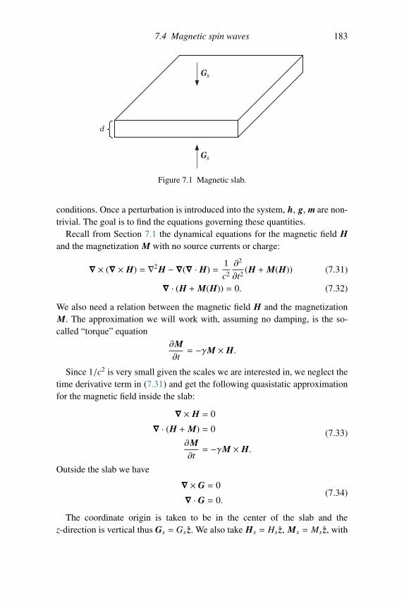
7.4 Magnetic spin waves 183
d
Gs
Gs
Figure 7.1 Magnetic slab.
conditions. Once a perturbation is introduced into the system, h, g, m are non-trivial. The goal is to find the equations governing these quantities.
Recall from Section 7.1 the dynamical equations for the magnetic field Hand the magnetization M with no source currents or charge:
∇ × (∇ × H) = ∇2H − ∇(∇ · H) =1c2
∂2
∂t2(H + M(H)) (7.31)
∇ · (H + M(H)) = 0. (7.32)
We also need a relation between the magnetic field H and the magnetizationM. The approximation we will work with, assuming no damping, is the so-called “torque” equation
∂M∂t= −γM × H.
Since 1/c2 is very small given the scales we are interested in, we neglect thetime derivative term in (7.31) and get the following quasistatic approximationfor the magnetic field inside the slab:
∇ × H = 0
∇ · (H + M) = 0
∂M∂t= −γM × H.
(7.33)
Outside the slab we have
∇ × G = 0
∇ · G = 0.(7.34)
The coordinate origin is taken to be in the center of the slab and thez-direction is vertical thus Gs = Gs z. We also take Hs = Hs z, Ms = Ms z, with
184 Nonlinear Schrodinger models in nonlinear optics
Gs, Hs, Ms all constant. The boundary conditions (since we have no sources)are derived from the continuity of the induction and magnetic fields that canbe written as
Hx = Gx, Hy = Gy, Hs + Ms = Gs all at z = ±d2.
It is convenient to introduce the scalar potentials ψ and φ as
h = ∇ψ,g = ∇φ.
Thus (7.33) and (7.34) can be reduced to
∂m∂t= −γ(Ms × h + m× Hs + m× h)
∇2ψ + ∇ · m = 0 (inside slab)
∇2φ = 0 (outside slab).
(7.35)
Suppose we assume a quasi-monochromatic wave expansion for thepotentials:
φ = ε(φ(1)eiθ + c.c.) + ε2(φ(0) + φ(2)e2iθ + c.c.) + · · ·
ψ = ε(ψ(1)eiθ + c.c.) + ε2(ψ(0) + ψ(2)e2iθ + c.c.) + · · ·
m = ε
⎛⎜⎜⎜⎜⎜⎜⎜⎜⎜⎝m(1)
1
m(1)20
⎞⎟⎟⎟⎟⎟⎟⎟⎟⎟⎠ (eiθ + c.c.) + · · · .
where θ = kx − ωt and φ( j), ψ( j), m( j) are slowly varying functions of x, t andare independent of y; i.e., φ( j) = φ( j)(X,T ), X = εx, T = εt, etc.
The first of (7.35) show that m(1)1 and m(1)
2 satisfy
−iωm(1)1 = −ωHm(2)
1 − iωm(2)1 = −ikωMψ
(1) + ωHm(1)1
where ωM = γMs, ωH = γHs. Hence
m(1)1 = χ1ikψ(1), m(1)
2 = −χ2kψ(1),
where
χ1 =ωHωM
ω2H − ω2
, χ2 =ωMω
ω2H − ω2
.
Exercises 185
To satisfy the latter two equations in (7.35) we find
φ(1) = A(X,T )e−k(|z|− d2 ) cos(k1d/2)
ψ(1) = A(X,T ) cos(k1z),
with
k21 = k2(1 + χ1).
Using continuity of the vertical fields, hz + mz = gz or ∂zψ = ∂zφ at z=± d/2,we find the dispersion relation
(1 + χ1)1/2 = cot(k1d/2),
which implicitly determines ω = ω(k). Finally we remark that at higher orderin the perturbation expansion, from a detailed calculation, an NLS equation forA = A(X,T ) is determined. For thin films (d � 1), the equation is found to be(see Zvezdin and Popkov, 1983)
i(AT + vgAX) + ε
(ω′′(k)
2AXX + n|A|2A
)= 0,
where n is a suitable function of k, γ, Hs, and Ms.
Exercises
7.1 (a) Derive the NLS equation (7.23) filling in the steps in the derivation.(b) Obtain an NLS equation in electromagnetic “bulk” media when
the slowly varying amplitude A in ( 7.15) is independent of T ;here the longitudinal direction plays the role of the the temporalvariable.
(c) Obtain the NLS equation in these (bulk) media when the slowlyvarying amplitude A in (7.15) is a function of X, Y , Z, T . Whathappens when A is independent of T?
7.2 (a) Derive the “NLSM system (7.29)–(7.30) by filling in the steps in thederivation.
(b) Derive time-independent systems similar to those discussed byAblowitz et al. (2005) (see also Chapter 6) by assuming the ampli-tude is steady; i.e., has no time dependence.
7.3 Assume quasi-monchromatic waves in both transverse dimensions andobtain a vector NLSM system in quadratic (χ(2) � 0) nonlinear opticalmedia. Hint: see Ablowitz et al. (1997, 2001a).
186 Nonlinear Schrodinger models in nonlinear optics
7.4 Use (7.35), and the assumed form of solution in that subsection, to obtainthe linear dispersion relation of a wave eikx−ωt) propagating in a ferro-magnetic strip of width d (like that depicted in Figure 7.1) but now withthe external magnetic field aligned along the:(a) x-axis;(b) y-axis.

PART II
INTEGRABILITY AND SOLITONS

8Solitons and integrable equations
In this chapter we begin by finding traveling wave solutions. We then discussthe so-called Miura transformation that is used to find an infinite num-ber of conservation laws and the associated linear scattering problem, thetime-independent Schrodinger scattering problem, for the Korteweg–de Vries(KdV) equation. Lax pairs and an expansion method that shows how com-patible linear problems are related to other nonlinear evolution equations aredescribed. An evolution operator, sometimes referred to as a recursion oper-ator, is also included. This operator can be used to find general classes ofintegrable nonlinear evolution equations. We point out that there are a num-ber of texts that discuss these matters (Ablowitz and Segur, 1981; Novikovet al., 1984; Calogero and Degasperis, 1982; Dodd et al., 1984; Faddeev andTakhtajan, 1987); we often follow closely the analytical development Ablowitzand Clarkson (1991).
8.1 Traveling wave solutions of the KdV equation
We begin with the Korteweg–de Vries equation in non-dimensional form
ut + 6uux + uxxx = 0. (8.1)
For the dimensional form of the equation we refer the reader to Chapter 1.An important property of the KdV equation is the existence of traveling wavesolutions, including solitary wave solutions. The solutions are written in termsof elementary or elliptic functions. Since a discussion of this topic appears inChapter 1 we will sometimes call on those results here.
A traveling wave solution of a PDE in one space, one time dimension, suchas the KdV equation, where t ∈ R, x ∈ R are temporal and spatial variablesand u ∈ R the dependent variable, has the form
189
190 Solitons and integrable equations
u(x, t) = w(x −Ct) = w(z). (8.2)
A solitary wave is a special traveling wave solution, which is bounded and hasconstant asymptotic states as z→ ∓∞.
To obtain traveling wave solutions of the KdV equation (8.1), we seek asolution in the form (8.2) that yields a third-order ordinary differential equationfor w
d3wdz3+ 6w
dwdz−C
dwdz= 0.
Integrating this once gives
d2wdz2+ 3w2 −Cw = E1, (8.3)
with E1 an arbitrary constant. Multiplying (8.3) by dw/dz and integrating againyields
12
(dwdz
)2= f (w) = −(w3 −Cw2/2 − E1w − E2), (8.4)
with E2 another arbitrary constant. We are interested in obtaining real, boundedsolutions for the KdV equation (8.1), so we require that f (w) ≥ 0. This leadsus to study the zeros of f (w). There are two cases to consider: when f (w) hasonly one real zero or when f (w) has three real zeros.
If f (w) has only one real zero, say w = α, so that f (w) = −(w − α)3, we canintegrate directly to find that
u(x, t) = w(x −Ct) = α − 2(x − 6αt − x0)2
.
So there are no bounded solutions in this case.On the other hand, if f (w) has three real zeros, which we take without loss
of generality to satisfy α ≤ β ≤ γ, then
f (w) = −(w − α)(w − β)(w − γ), (8.5)
where γ = 2(α + β + γ), E1 = −2(αβ + βγ + γα), E2 = 2αβγ.Suppose α, β, γ are distinct; then the solution of the KdV equation may
be expressed in terms of the Jacobian elliptic function cn(z; m) (see alsoChapter 1)
u(x, t) = w(x −Ct)= β + (γ − β) cn2{[
12 (γ − α)
]1/2[x −Ct − x0] ; m
},
(8.6)
8.1 Traveling wave solutions of the KdV equation 191
with
C = 2(α + β + γ), m =γ − βγ − α, where 0 < m < 1, (8.7)
x0 is a constant and m denotes the modulus of the Jacobian elliptic function.These solutions of the KdV equation were originally found by Korteweg andde Vries; in fact they called these solutions cnoidal waves. Since cn(z; m) hasperiod [z] = 4K(m) where K is the complete elliptic integral of the first kind,we have that the period of u(x, t) is [x] = L = 2K(m)/
(12 (γ − α)
).
Noting that cn(z; m) = cos(z) + O(m) for m � 1 (β→ γ), it follows that
u(x, t) = w(x −Ct) ∼ 12 (β + γ) +
γ − β2
cos {2κ[x −Ct − x0]} ,
where κ2 = 12 (γ − α), C ≈ 2(α − 2β). Thus when γ → β we have the limiting
case of a sinusoidal wave.Next suppose in (8.6), (8.7) we take the limit β → α (i.e., m → 1), with
β � γ; then since cn(z; 1) = sech(z) it reduces to the solitary wave solution
u(x, t) = w(x −Ct) = β + 2κ2 sech2{κ[x − (4κ2 + 6βu0)t + δ0]
}(8.8)
where κ2 = 12 (γ − β).
It then follows that the speed of the wave relative to the uniform state u0
is related to the amplitude: bigger solitary waves move faster than smallerones. Note, if β = 0 (α = 0), then the wave speed is twice the amplitude.It is also clear that the amplitude 2κ2 is independent of the uniform back-ground β. Finally the width of the solitary wave is inversely proportional toκ; hence narrower solitary waves are taller and faster. We note that these soli-tary waves are consistent with the observations of J. Scott Russell mentioned inChapter 1.
If α < β = γ, then the solution of (8.6) is given by
u(x, t) = w(x −Ct),
= β − (β − α) sec2{[
12 (β − α)
]1/2[x − 2(α + 2β)t − x0]
}[this can be obtained by using (8.5) and directly integrating], where x0
is a constant. This solution is unbounded unless α = β in which caseu = u0 = β.
192 Solitons and integrable equations
8.2 Solitons and the KdV equation
As discussed in Chapter 1, the physical model that motivated the recentdiscoveries associated with the KdV equation (1.5) was a problem of a one-dimensional anharmonic lattice of equal masses coupled by nonlinear stringsthat remarkably was studied numerically by Fermi, Pasta and Ulam (FPU).
The FPU model consisted of identical masses, m, connected by nonlinearsprings with the force law F(Δ) = −k(Δ + αΔp), with k > 0, α being springconstants:
md2yn
dt2= k[yn+1 − yn + α(yn+1 − yn)p] − k[yn − yn−1 + α(yn − yn−1)p]
= k(yn+1 − 2yn + yn−1) + kα[(yn+1 − yn)p − (yn − yn−1)p](8.9)
for n = 1, 2, . . . ,N − 1, with y0 = 0 = yN and initial condition yn(0) =sin(nπ/N), yn,t(0) = 0.
In 1965, Zabusky and Kruskal transformed the differential-difference equa-tion (8.9) to a continuum model and studied the case p = 2. Calling the lengthbetween springs h, t = ωt (with ω =
√K/m), x = x/h with x = nh and
expanding yn±1 in a Taylor series, then (dropping the tildes) (8.9) reduces to
ytt = yxx + εyxyxx +1
12 h2yxxxx + O(εh2, h4), (8.10)
where ε = 2αh. They found (see Chapter 1) an asymptotic reduction by lookingfor a solution of the form (unidirectional waves)
y(x, t) ∼ φ(ξ, τ), ξ = x − t, τ = 12εt,
whereupon (8.10), with u = φξ, and ignoring small terms, where δ2 = h2/12ε,reduces to the KdV equation [with different coefficients from (8.1)]
uτ + uuξ + δ2uξξξ = 0. (8.11)
It is also noted that when the force law is taken as F(Δ) = −k(Δ + αΔp) withp = 3 then, after rescaling, one obtains the modified KdV (mKdV) equation(see also the next section)
uτ + u2uξ + δ2uξξξ = 0.
We saw earlier that the KdV equation possesses a solitary wave solution;see (8.8). Although solitary wave solutions of the KdV equation had beenwell known for a long time, it was not until Zabusky and Kruskal, in 1965,did extensive numerical studies for the KdV equation (8.11) that the remark-able properties of the solitary waves associated with the KdV equation were
8.3 Miura transformation and conservation laws 193
discovered. Zabusky and Kruskal considered the initial value problem for theKdV equation (8.11) with (δ2 � 1) the initial condition
u(ξ, 0) = cos(πξ), 0 ≤ ξ ≤ 2,
where u, uξ, uξξ are periodic on [0, 2] for all t. As also described in Chapter1, they found that after a short time the wave steepens and almost produces ashock, but the dispersive term δ2uxxx then becomes significant and a balancebetween the nonlinear and dispersion terms ensues. Later the solution devel-ops a train of (eight) well-defined waves, each like a solitary wave (i.e., sech2
functions), with the faster (taller) waves catching up and overtaking the slower(smaller) waves.
From this they observed that when two solitary waves with different wavespeeds are initially well separated, with the larger one to the left (the wavesare traveling from left to right), then the faster, taller wave catches up andsubsequently overlaps the slower, smaller one; the waves interact nonlinearly.After the interaction, they found that the waves separate, with the larger onein front and slower one behind, but both having regained the same amplitudesthey had before the interactions, the only effect of the interaction being a phaseshift; that is, the centers of the waves are at different positions than where theywould have been had there been no interaction. Thus they deduced that thesenonlinear solitary waves essentially interacted elastically. Making the analogywith particles, Zabusky and Kruskal called these special waves solitons.
Mathematically speaking, a soliton is a solitary wave that asymptoticallypreserves its shape and velocity upon nonlinear interaction with other solitarywaves, or more generally, with another (arbitrary) localized disturbance.
In the physics literature the term soliton is often meant to be a solitary wavewithout the elastic property. When dealing with physical problems in order tobe consistent with what is currently accepted, we frequently refer to solitonsin the latter sense (i.e., solitary waves without the elastic property).
Kruskal and Zabusky’s remarkable numerical discovery demanded an ana-lytical explanation and a detailed mathematical study of the KdV equation.However the KdV equation is nonlinear and at that time no general method ofsolution for nonlinear equations existed.
8.3 The Miura transformation and conservation lawsfor the KdV equation
We have seen that the KdV equation arises in the description of physicallyinteresting phenomena; however interest in this nonlinear evolution equation
194 Solitons and integrable equations
is also due to the fact that analytical developments have led researchers toconsider the KdV equation to be an integrable or sometimes referred to asan exactly solvable equation. This terminology is a consequence of the factthat the initial value problem corresponding to appropriate data (e.g., rapidlydecaying initial data) for the KdV equation can be “solved exactly”, or moreprecisely, linearized by a method that employs inverse scattering. The inversescattering method was discovered by Gardner, Greene, Kruskal and Miura(1967) as a means for solving the initial value problem for the KdV equationon the infinite line, for initial values that decay sufficiently rapidly at infin-ity. Subsequently this method has been significantly enhanced and extendedby many researchers and is usually termed the inverse scattering transform(IST) (cf. Ablowitz and Segur, 1981; Ablowitz and Clarkson, 1991; Ablowitzet al., 2004b). We also note that Lax and Levermore (1983a,b,c) and Venakides(1985) have reinvestigated (8.11) with δ small; that leads to an understandingof the weak limit of KdV.
The KdV equation has several other remarkable properties beyond the exis-tence of solitons (discussed earlier), including the possession of an infinitenumber of polynomial conservation laws. Discovering this was important inthe development of the general method of solution for the KdV equation.
Associated with a partial differential equation denoted by
F[x, t; u(x, t)] = 0, (8.12)
where t ∈ R, x ∈ R are temporal and spatial variables and u(x, t) ∈ R thedependent variable (in the argument of F additional partial derivatives of u areunderstood) may be a conservation law; that is, an equation of the form
∂tTi + ∂xXi = 0, (8.13)
that is satisfied for all solutions of (8.12). Here Ti(x, t; u), called the conserveddensity, and Xi(x, t; u), the associated flux, are, in general, functions of x, t, uand the partial derivatives of u – see also Chapter 2.
If additionally, u → 0 as |x| → ∞ sufficiently rapidly, then by integrat-ing (8.13) we get
ddt
∫ ∞
−∞Ti(x, t; u) dx = 0
in which case ∫ ∞
−∞Ti(x, t; u) dx = ci,
where ci, constant, is called the conserved quantity.
8.3 Miura transformation and conservation laws 195
For the KdV equation (1.5), the first three conservation laws are
(u)t + (3u2 + uxx)x = 0,
(u2)t +(4u3 + 2uuxx − u2
x
)x= 0,(
u3 − 12 u2
x
)t+(
92 u4 + 3u2uxx − 6uu2
x − uxuxxx +12 u2
xx
)x= 0.
The first two of these correspond to conservation of mass (or sometimesmomentum) and energy, respectively. The third is related to the Hamiltonian(Whitham, 1965). The fourth and fifth conservation laws for the KdV equa-tion were found by Kruskal and Zabusky. Subsequently some additional oneswere discovered by Miura and it was conjectured that there was an infinitenumber.
After studying these conservation laws of the KdV equation and those asso-ciated with another equation, the so-called modified KdV (mKdV) equationthat we write as
mt − 6m2mx + mxxx = 0, (8.14)
Miura (1968) discovered that with a solution m of (8.14), then u given by
u = −m2 − mx, (8.15)
is a solution of the KdV equation (8.1). Equation (8.15) is known as the Miuratransformation. Direct substitution of (8.15) into (1.5) yields
ut + 6uux + uxxx = −(m2 + mx
)t+ 6(m2 + mx
) (m2 + mx
)x−(m2 + mx
)xxx
= − (2mmt + mxt) + 6(m2 + mx
)(2mmx + mxx)
− (2mmxxx + 6mxmxx + mxxxx)
= −(mxt − 6m2mxx − 12mm2
x + vxxxx
)− (2mmt − 12m3mx + 2mmxxx)
= −(2m + ∂x)(mt − 6m2mx + mxxx)
= −(2m + ∂x)(mt − 6m2mx + mxxx
).
Note that every solution of the mKdV equation (8.14) leads, via Miura’s trans-formation (8.15), to a solution of the KdV equation, but the converse is nottrue; i.e., not every solution of the KdV equation can be obtained from a solu-tion of the mKdV equation – see, for example, Ablowitz, Kruskal and Segur(1979). Miura’s transformation leads to many other important results relatedto the KdV equation. Initially it formed the basis of a proof that the KdV andmKdV equations have an infinite number of conserved densities (Miura et al.,1968), which is outlined below. Importantly, Miura’s transformation (8.15) was
196 Solitons and integrable equations
also critical in the development of the inverse scattering method or inversescattering transform (IST) for solving the initial value problem for the KdVequation (8.1) – details are in the next chapter.
To show that the KdV equation admits an infinite number of conservationlaws, define a variable w by the relation
u = w − εwx − ε2w2, (8.16)
which is a generalization of Miura’s transformation (8.15).1 Then the equiva-lent relation is
ut + 6uux + uxxx =(1 − ε∂x − 2ε2w
)(wt + 6(w − ε2w2)wx + wxxx).
Therefore u, as defined by (8.16), is a solution of the KdV equation providedthat w is a solution of
wt + 6(w − ε2w2)wx + wxxx = wt + ∂x(3w2 − 2w3 + wxx) = 0. (8.17)
Since the KdV equation does not contain ε, then its solution u depends onlyupon x and t. However w, a solution of (8.17), depends on x, t and ε. Since εis arbitrary we can seek a formal power series solution of (8.16), in the form
w(x, t; ε) =∞∑
n=0
wn(x, t)εn. (8.18)
The equation (8.17) is in conservation form, thus∫ ∞
−∞w(x, t; ε) dx = constant,
and so ∫ ∞
−∞wn(x, t) dx = constant,
for each n = 0, 1, 2, . . . . Substituting (8.18) into (8.16), equating coefficientsof powers of ε and solving recursively gives
w0 = u,
w1 = w0,x = ux,
w2 = w1,x + w20 = uxx + u2,
w3 = w2,x + 2w0w1 = uxxx + 4uux = (uxx + 2u2)x ,
w4 = w3,x + 2w0w2 + w21 = uxxxx + 6uuxx + 5u2
x + 2u3,
(8.19)
1 Taking m = εw − 1/ε and performing a Galilean transformation.
8.4 Time-independent Schrodinger equation 197
etc. Continuing to all powers of ε gives an infinite number of conserveddensities. The corresponding conservation laws may be found by substitut-ing (8.18)–(8.19) into (8.17) and equating coefficients of powers of ε. Wefurther note that odd powers of ε are trivial since they are exact derivatives. Sothe even powers give the non-trivial conservation laws for the KdV equation.
8.4 Time-independent Schrodinger equation and acompatible linear system
The Miura transformation (8.15) may be viewed as a Riccati equation for min terms of u. It is well known that it may be linearized by the transformationm = vx/v, which yields
u + m2 + mx = u +v2
x
v2+
(vxx
v− v2
x
v2
)= 0,
and so u = −vxx/v or
vxx + uv = 0. (8.20)
This is reminiscent of the Cole–Hopf transformation (see Section 3.6). How-ever, (8.20) does not yield an explicit linearization for the KdV equation. Muchmore must be done. Since the KdV equation is Galilean invariant – that is, it isinvariant under the transformation
(x, t, u(x, t))→ (x − 6λt, t, u(x, t) + λ) ,
where λ is some constant – then it is natural to consider
Lv := vxx + u(x, t)v = λv. (8.21)
This equation is the time-independent Schrodinger equation that has beenextensively studied by mathematicians and physicists; we note that here t playsthe role of a parameter and u(x, t) the potential.
The associated time dependence of the eigenfunctions of (8.21) is given by
vt = (γ + ux)v − (4λ + 2u)vx, (8.22)
where γ is an arbitrary constant. This form is different from the original onefound by Gardner, Greene, Kruskal and Miura (1967); see also Gardner et al.(1974): it is simpler and leads to the same results. Then if λ = λ(t) from (8.21)and (8.22) we obtain
vtxx =[(γ + ux)(λ − u) + uxxx + 6uux
]v − (4λ + 2u)(λ − u)vx,
vxxt =[(λ − u)(γ + ux) − ut + λt
]v − (λ − u)(4λ + 2u)vx.
198 Solitons and integrable equations
Therefore (8.21) and (8.22) are compatible, i.e., vxxt = vtxx, if λt = 0 and usatisfies the KdV equation (1.5). Similarly, if (1.5) is satisfied, then necessarilythe eigenvalues must be time independent (i.e., λt = 0).
It turns out that the eigenvalues and the behavior of the eigenfunctionsof the scattering problem (8.21) as |x| → ∞, determine the scattering data,S (λ, t), which in turn depends upon the potential u(x, t). The direct scatteringproblem is to map the potential into the scattering data. The time evolutionequation (8.22) takes initial scattering data S (λ, t = 0) to data at any timet, i.e., to S (λ, t). The inverse scattering problem is to reconstruct the poten-tial from the scattering data. The details of the solution method of the KdVequation (8.1) are described in the next chapter.
8.5 Lax pairs
Recall that the operators associated with the KdV equation are
Lv = vxx + u(x, t)v = λv,
vt =Mv = (ux + γ)v − (2u + 4λ)vx,
where γ is an arbitrary constant parameter and λ is a spectral parameter thatis constant (λt = 0). We found that these equations are compatible (i.e., vxxt =
vtxx) provided that u satisfies the KdV equation (8.1).Lax (1968) put the inverse scattering method for solving the KdV equation
into a more general framework that subsequently paved the way to gener-alizations of the technique as a method for solving other partial differentialequations. Consider two operators L and M, where L is the operator of thespectral problem andM is the operator governing the associated time evolutionof the eigenfunctions
Lv = λv, (8.23)
vt =Mv. (8.24)
Now take ∂/∂t of (8.23), giving
Ltv +Lvt = λtv + λvt;
hence using (8.24)
Ltv +LMv = λtv + λMv,
= λtv +Mλv,
= λtv +MLv.
8.6 Linear scattering problems 199
Therefore we obtain
[Lt + (LM−ML)] v = λtv,
and hence in order to solve for non-trivial eigenfunctions v(x, t)
Lt + [L,M] = 0, (8.25)
where
[L,M] := LM−ML,if and only if λt = 0. Equation (8.25) is sometime called Lax’s equation andL, M are called the Lax pair. Furthermore, (8.25) contains a nonlinear evolu-tion equation for suitably chosen L andM. For example, if we take [suitablyreplacing λ by ∂2
x + u in (8.24)]
L = ∂2
∂x2+ u, (8.26)
M = γ − 3ux − 6u∂
∂x− 4
∂3
∂x3, (8.27)
then L andM satisfy (8.25) and u satisfies the KdV equation (8.1). Therefore,the KdV equation may be thought of as the compatibility condition of the twolinear operators given by (8.26), (8.27). As we will see below, there is a generalclass of equations that are associated with the Schrodinger operator (8.26).
8.6 Linear scattering problems and associated nonlinearevolution equations
Following the development of the method of inverse scattering for the KdVequation by Gardner, Greene, Kruskal and Miura (1967), it was then of consid-erable interest to determine whether the method would be applicable to otherphysically important nonlinear evolution equations. The method was thoughtto possibly only apply to one physically important equation; perhaps it wasanalogous to the Cole–Hopf transformation (Cole, 1951; Hopf, 1950) thatlinearizes Burgers’ equation (see Chapter 3)
ut + 2uux − uxx = 0.
Namely, if we make the transformation u = −φx/φ, then φ(x, t) satisfies thelinear heat equation φt − φxx = 0. [We remark that Forsyth (1906) first pointedout the relationship between Burgers’ equation and the linear heat equa-tion]. But Burgers’ equation is the only known physically significant equationlinearizable by the above transformation.
200 Solitons and integrable equations
However, Zakharov and Shabat (1972) proved that the method wasindeed more general. They extended Lax’s method and related the nonlinearSchrodinger equation
iut + uxx + κu2u∗ = 0, (8.28)
where ∗ denotes the complex conjugate and κ is a constant, to a certain linearscattering problem or Lax pairs where nowL andM are 2×2 matrix operators.Using these operators, Zakharov and Shabat were able to solve (8.28), giveninitial data u(x, 0) = f (x), assuming that f (x) decays sufficiently rapidly as|x| → ∞. Shortly thereafter, Wadati (1974) found the method of solution forthe modified KdV equation
ut − 6u2ux + uxxx = 0, (8.29)
and Ablowitz, Kaup, Newell and Segur (1973a), motivated by some importantobservations by Kruskal, solved the sine–Gordon equation:
uxt = sin u. (8.30)
Ablowitz, Kaup, Newell and Segur (1973b, 1974) then developed a generalprocedure, which showed that the initial value problem for a remarkably largeclass of physically interesting nonlinear evolution equations could be solved bythis method. There is also an analogy between the Fourier transform methodfor solving the initial value problem for linear evolution equations and theinverse scattering method. This analogy motivated the term: inverse scatteringtransform (IST) (Ablowitz et al., 1974) for the new method.
8.6.1 Compatible equations
Next we outline a convenient method for finding “integrable” equations.Consider two linear equations
vx = Xv, vt = Tv, (8.31)
where v is an n-dimensional vector and X and T are n×n matrices. If we requirethat (8.31) are compatible – that is, requiring that vxt = vtx – then X and T mustsatisfy
Xt − Tx + [X,T] = 0. (8.32)
Equation (8.32) and Lax’s equation (8.26), (8.27) are similar; equation (8.31)is somewhat more general as it allows more general eigenvalue dependenceother than Lv = λv.
8.6 Linear scattering problems 201
The method is sometimes referred to as the AKNS method (Ablowitz et al.,1974). As an example, consider the 2 × 2 scattering problem [this is a general-ization of the Lax pair studied by Zakharov and Shabat (1972)] given by (withthe eigenvalue denoted as k)
v1,x = −ikv1 + q(x, t)v2,
v2,x = ikv2 + r(x, t)v1,(8.33)
with the linear time dependence given by
v1,t = Av1 + Bv2,
v2,t = Cv1 + Dv2,(8.34)
where A, B, C and D are scalar functions of q(x, t), r(x, t), and their derivatives,and k. In terms of X and T, we specify that
X =
(−ik qr ik
), T =
(A BC D
).
Note that if there were any x-derivatives on the right-hand side of (8.34)then they could be eliminated by use of (8.33). Furthermore, when r = −1,then (8.33) reduces to the Schrodinger scattering problem
v2,xx + (k2 + q)v2 = 0. (8.35)
It is interesting to note that physically interesting nonlinear evolution equationsarise from this procedure when either r = −1 or r = q∗ (or r = q if q is real).
This method provides an elementary technique that allows us to find nonlin-ear evolution equations. The compatibility of (8.33)–(8.34) – that is, requiringthat v j,xt = v j,tx, for j = 1, 2 – and the assumption that the eigenvalue k is time-independent – that is, dk/dt = 0 – imposes a set of conditions that A, B, C andD must satisfy. Sometimes the nonlinear evolution equations obtained this wayare referred to as isospectral flows. Namely,
v1,xt = −ikv1,t + qtv2 + qv2,t,
= −ik(Av1 + Bv2) + qtv2 + q(Cv1 + Dv2),
v1,tx = Axv1 + Av1,x + Bxv2 + Bv2,x,
= Axv1 + A(−ikv1 + qv2) + Bxv2 + B(ikv2 + rv1).
Hence by equating the coefficients of v1 and v2, we obtain
Ax = qC − rB,
Bx + 2ikB = qt − (A − D)q,(8.36)
202 Solitons and integrable equations
respectively. Similarly
v2,xt = ikv2,t + rtv1 + rv1,t,
= ik(Cv1 + Dv2) + rtv1 + a(A1 + Bv2),
v2,tx = Cxv1 +Cv1,x + Dxv2 + Dv2,x,
= Cxv1 +C(−ikv1 + qv2) + Dxv2 + D(ikv2 + rv1),
and equating the coefficients of v1 and v2 we obtain
Cx − 2ikC = rt + (A − D)r,
(−D)x = qC − rB.(8.37)
Therefore, from (8.36), without loss of generality, we may assume D = −A,and hence it is seen that A, B and C necessarily satisfy the compatibilityconditions
Ax = qC − rB,
Bx + 2ikB = qt − 2Aq,
Cx − 2ikC = rt + 2Ar.
(8.38)
We next solve (8.38) for A, B and C, thus ensuring that (8.33) and (8.34) arecompatible. In general, this can only be done if another condition (on r and q)is satisfied, this condition being the evolution equation. Since k, the eigenvalue,is a free parameter, we may find solvable evolution equations by seeking finitepower series expansions for A, B and C:
A =n∑
j=0
Ajkj, B =
n∑j=0
Bjkj, C =
n∑j=0
C jkj. (8.39)
Substituting (8.39) into (8.38) and equating coefficients of powers of k, weobtain 3n+5 equations. There are 3n+3 unknowns, Aj, Bj, C j, j = 0, 1, . . . , n,and so we also obtain two nonlinear evolution equations for r and q. Now letus consider some examples.
Example 8.1 n = 2. Suppose that A, B and C are quadratic polynomials,that is
A = A2k2 + A1k + A0,
B = B2k2 + B1k + B0,
C = C2k2 +C1k +C0.
(8.40)
Substitute (8.40) into (8.38) and equate powers of k. The coefficients of k3
immediately give B2 = C2 = 0. At order k2, we obtain A2 = a, a constant(we could have allowed a to be a function of time, but for simplicity we donot do so), B1 = iaq, C1 = iar. At order k1, we obtain A1 = b, constant, and
8.6 Linear scattering problems 203
for simplicity we set b = 0 (if b � 0 then a more general evolution equationis obtained); then B0 = − 1
2 aqx and C0 =12 arx. Finally, at order k0, we obtain
A0 =12 arq + c, with c a constant (again for simplicity we set c = 0). Therefore
we obtain the following evolution equations
− 12 aqxx = qt − aq2r,12 arxx = rt + aqr2.
(8.41)
If in (8.41) we set r = ∓q∗ and a = 2i, then we obtain the nonlinear Schrodingerequation
iqt = qxx ± 2q2q∗. (8.42)
for both focusing (+) and defocusing (−) cases. In summary, setting r = ∓q∗,we find that
A = 2ik2 ∓ iqq∗,
B = 2qk + iqx,
C = ±2q∗k ∓ iq∗x
(8.43)
satisfy (8.38) provided that q(x, t) satisfies the nonlinear Schrodinger equa-tion (8.42).
Example 8.2 n = 3. If we substitute the following third-order polynomi-als in k
A = a3k3 + a2k2 + 12 (a3qr + a1)k + 1
2 a2qr − 14 ia3(qrx − rqx) + a0,
B = ia3qk2 +(ia2q − 1
2 a3qx
)k +[ia1q − 1
2 a2qx +14 ia3(2q2r − qxx)
],
C = ia3rk2 +(ia2r + 1
2 a3rx
)k +[ia1r + 1
2 a2rx +14 ia3(2r2q − rxx)
],
into (8.38), with a3, a2, a1 and a0 constants, then we find that q(x, t) and r(x, t)satisfy the evolution equations
qt +14 ia3(qxxx − 6qrqx) + 1
2 a2(qxx − 2q2r) − ia1qx − 2a0q = 0,
rt +14 ia3(rxxx − 6qrrx) − 1
2 a2(rxx − 2qr2) − ia1rx + 2a0r = 0.(8.44)
For special choices of the constants a3, a2, a1 and a0 in (8.44) we find phys-ically interesting evolution equations. If a0 = a1 = a2 = 0, a3 = −4i andr = −1, then we obtain the KdV equation
qt + 6qqx + qxxx = 0.
If a0 = a1 = a2 = 0, a3 = −4i and r = q, then we obtain the mKdV equation
qt − 6q2qx + qxxx = 0.
[Note that if a0 = a1 = a3 = 0, a2 = −2i and r = −q∗, then we obtain thenonlinear Schrodinger equation (8.42).]
204 Solitons and integrable equations
We can also consider expansions of A, B and C in inverse powers of k.
Example 8.3 n = −1. Suppose that
A =a(x, t)
k, B =
b(x, t)k
, C =c(x, t)
k;
then the compatibility conditions (8.38) are satisfied if
ax =i2 (qr)t, qxt = −4iaq, rxt = −4iar.
Special cases of these are
(i)
a = 14 i cos u, b = −c = 1
4 i sin u, q = −r = − 12 ux :
then u satisfies the sine–Gordon equation
uxt = sin u.
(ii)
a = 14 i cosh u, b = −c = − 1
4 i sinh u, q = r = 12 ux,
where u satisfies the sinh–Gordon equation:
uxt = sinh u.
These examples only show a few of the many nonlinear evolution equationsthat may be obtained by this procedure. We saw above that when r = −1, thescattering problem (8.33) reduced to the Schrodinger equation (8.35). In thiscase we can take an alternative associated time dependence
vt = Av + Bvx.
By requiring that this and (λ = k2)
vxx + (λ + q)v = 0
are compatible and assuming that dλ/dt = 0, yields equations for A and Banalogous to (8.38), then by expanding in powers of λ, we obtain a generalclass of equations.
8.7 More general classes of nonlinear evolution equations 205
8.7 More general classes of nonlinear evolution equations
A natural question is: what is a general class of “solvable” nonlinear evolutionequations? Here we use the 2 × 2 scattering problem
v1,x = −ikv1 + q(x, t)v2, (8.45a)
v2,x = −ikv2 + r(x, t)v1, (8.45b)
to investigate this issue. Ablowitz, Kaup, Newell and Segur (1974) answeredthis question by considering the equations (8.45) associated with the functionsA, B and C in (8.34). Under certain restrictions, a relation was found that givesa class of solvable nonlinear equations. This relationship depends upon the dis-persion relation of the linearized form of the nonlinear equations and a certainintegro-differential operator. Suppose that q and r vanish sufficiently rapidly as|x| → ∞: then a general evolution equation can be shown to be(
r−q
)t
+ 2A0(L)
(rq
)= 0 (8.46a)
where A0(k) = lim|x|→∞ A(x, t, k) (we may think of A0(k) as the ratio of twoentire functions), and L is the integro-differential operator given by
L =12i
(∂x − 2r(I−q) 2r(I−r)−2q(I−q) −∂x + 2q(I−r)
), (8.46b)
where ∂x ≡ ∂/∂x and
(I− f )(x) ≡∫ x
−∞f (y)dy. (8.46c)
Note that L operates on (r, q), and I− operates both on the functions immedi-ately to its right and also on the functions to which L is applied. Equation (8.46)may be written in matrix form
σ3ut + 2A0(L)u = 0,
where
σ3 =
(1 00 −1
), u =
(rq
).
It is significant that A0(k) is closely related to the dispersion relation of theassociated linearized problem. If f (x) and g(x) vanish sufficiently rapidly as|x| → ∞, then in the limit |x| → −∞,
f (x)(I−g)(x) ≡ f (x)∫ x
−∞g(y)dy→ 0,
206 Solitons and integrable equations
and so for infinitesimal q and r, we have that L is the diagonal differentialoperator
L =12i
∂
∂x
(1 00 −1
).
Hence in this limit (8.46) yields
rt + 2A0
(−1
2i∂x
)r = 0,
−qt + 2A0
(12
i∂x
)q = 0.
The above equations are linear (decoupled) partial differential equations solv-able by Fourier transform methods. Substituting the wave solutions r(x, t) =exp(i(kx −ωr(2k)t)), q(x, t) = exp(i(kx −ωq(−2k)t)), into the above equations,we obtain the relationship
A0(k) =12
iωr(2k) = −12
iωq(−2k). (8.47)
Therefore a general evolution equation is given by(r−q
)= −iω(2L)
(rq
)(8.48)
with ωr(k) = ω(k); in matrix form this equation takes the form
σ3ut + iω(2L)u = 0.
Hence, the form of the nonlinear evolution equation is characterized bythe dispersion relation of its associated linearized equations and an integro-differential operator; further details can be found in Ablowitz et al. (1974).
For the nonlinear Schrodinger equation
iqt = qxx ± 2q2q∗, (8.49)
the associated linear equation is
iqt = qxx.
Therefore the dispersion relation is ωq(k) = −k2, and so from (8.47), A0(k) isgiven by
A0(k) = 2ik2. (8.50)
The evolution is obtained from either (8.46) or (8.48); therefore we have(r−q
)t
= −4iL2
(rq
)= −2L
(rx
qx
)= i
(rxx − 2r2qqxx − 2q2r
).
8.7 More general classes of nonlinear evolution equations 207
When r = ∓q∗, both of these equations are equivalent to the nonlinearSchrodinger equation (8.49). Note that (8.50) is in agreement with (8.41) witha = 2i (that is lim|x|→∞ A = 2ik2, since lim|x|→∞ r(x, t) = 0). This explainsa posteriori why the expansion of A, B and C in powers of k are related soclosely to the dispersion relation. Indeed, now in retrospect, the fact that thenonlinear Schrodinger equation is related to (8.50) implies that an expansionstarting at k2 will be a judicious choice. Similarly, the modified KdV equationand sine–Gordon equation can be obtained from the operator equation (8.48)using the dispersion relations ω(k) = −k3 and ω(k) = k−1, respectively. Thesedispersion relations suggest expansions commencing in powers of k3 and k−1,respectively, that indeed we saw to be the case in the earlier section.
The derivation of (8.48) required that q and r tend to 0 as |x| → 0 andtherefore we cannot simply set r = −1 in order to obtain the equivalent resultfor the Schrodinger scattering problem
vxx + (k2 + q)v = 0. (8.51)
However the essential ideas are similar and Ablowitz, Kaup, Newell and Segur(1974) also showed that a general evolution equation in this case is
qt + γ(L)qx = 0, (8.52a)
where
L ≡ −14∂2
x − q +12
qxI+, (8.52b)
I+ f (x) ≡∫ ∞
xf (y)dy. (8.52c)
γ(k2) =ω(2k)
2k, (8.52d)
with ∂x = ∂/∂x and ω(k), is the dispersion relation of the associated linearequation with q = exp(i(kx − ω(k)t)).
For the KdV equation
qt + 6qqx + qxxx = 0,
the associated linear equation is
qt + qxxx = 0.
Therefore ω(k) = −k3 and so γ(k2) = −4k2, thus γ(L) = −4L. Hence (8.52)yields
qt − 4Lqx = 0,
208 Solitons and integrable equations
thus
qt − 4
(−1
4∂2
x − q +12
qxI+
)qx = 0,
which is the KdV equation!Associated with the operator L there is a hierarchy of equations (sometimes
referred to as the Lenard hierarchy) given by
ut + Lkux = 0, k = 1, 2, . . .
The first two subsequent higher-order equations in the KdV hierarchy are givenby
ut − 14
(u5x + 10uu3x + 20uxuxx + 30u2ux
)= 0,
ut +1
16(u7x + 14uu5x + 42uxu4x + 70uxxu3x + 70u2u3x
+280uuxuxx + 70u3x + 140u3nx
)= 0
where unx = ∂nu/∂xn.
In the above we studied two different scattering problems, namely theclassical time-independent Scrodinger equation
vxx + (u + k2)v = 0, (8.53)
which can be used to linearize the KdV equation, and the 2 × 2 scatteringproblem
vx = k
( −i 00 i
)v +(
0 qr 0
)v, (8.54)
which can linearize the nonlinear Schrodinger, mKdV and Sine–Gordon equa-tions. While (8.53) can be interpreted as a special case of (8.54), from thepoint of view of possible generalizations, however, we regard them as differentscattering problems.
There have been numerous applications and generalizations of this methodonly a few of which we will discuss below. One generalization includes thatof Wadati et al. (1979a,b) (see also Shimizu and Wadati, 1980; Ishimori, 1981,1982; Wadati and Sogo, 1983; Konno and Jeffrey, 1983). For example, insteadof (8.33), suppose we consider the scattering problem
v1,x = − f (k)v1 + g(k)q(x, t)v2,
v2,x = f (k)v2 + g(k)r(x, t)v1,(8.55)
8.7 More general classes of nonlinear evolution equations 209
where f (k) and g(k) are polynomial functions of the eigenvalue k, and the timedependence is given (as previously) by
v1,t = Av1 + Bv2,
v2,t = Cv1 + Dv2.(8.56)
The compatibility of (8.55) and (8.56) requires that A, B, C, D satisfy linearequations that generalize equations (8.36)–(8.38).
As earlier, expanding A, B, C, f and g in finite power series expansionsin k (where the expansions for f and g have constant coefficients), then oneobtains a variety of physically interesting evolution equations (cf. Ablowitzand Clarkson, 1991, for further details).
Extensions to higher-order scattering problems have been considered by sev-eral authors. There are two important classes of one-dimensional linear scat-tering problems, associated with the solvable nonlinear evolution equations:scalar and systems of equations. Some generalizations are now mentioned.
Ablowitz and Haberman (1975) studied an N × N matrix generalization ofthe scattering problem (8.54):
∂v∂x= ikJv +Qv, (8.57a)
where the matrix of potentials Q(x) ∈ MN(C) (the space of N × N matricesover C) with Qii = 0, J = diag(J2, J2, . . . , JN), where Ji � J j for i � j,i, j = 1, 2, . . . ,N, and v(x, t) is an N-dimensional vector eigenfunction. In thiscase, to obtain evolution equations, the associated time dependence is chosento be
∂v∂t= Tv, (8.57b)
where T is also an N × N matrix. The compatibility of (8.57) yields
Tx = Qt + ik[J,T] + [Q,T].
In the same way for the 2 × 2 case discussed earlier in the chapter, associatednonlinear evolution equations may be found by assuming an expansion for Tin powers or inverse powers of the eigenvalue k
T =n∑
j=0
k jT j. (8.58)
Ablowitz and Haberman showed that this scattering problem can be used tosolve several physically interesting equations such as the three-wave inter-action equations in one spatial dimension (with N = 3 and n = 1) and the
210 Solitons and integrable equations
Boussinesq equation (with N = 3 and n = 2). The associated recursion oper-ators have been obtained by various authors, cf. Newell (1978) and Fokas andAnderson (1982). The inverse problem associated with the scattering prob-lem (8.57) in the general N × N case has been rigorously studied by Bealsand Coifman (1984, 1985), Caudrey (1982), Mikhailov (1979, 1981) and Zhou(1989).
The following Nth order generalization of the scattering problem (8.53) wasconsidered by Gel’fand and Dickii (1977)
dNvdxN+
N∑j=2
u j(x)dN− jvdxN− j
= λv, (8.59)
where uj(x) are considered as potentials; they investigated many of the alge-braic properties of the nonlinear evolution equations solvable through thisscattering problem. The general inverse problem associated with this scatter-ing problem is treated in detail in the monograph of Beals, Deift, and Tomei(1988).
The scattering problems (8.53) and (8.54), and their generalizations (8.59)and (8.57), are only some of the examples of scattering problems used inconnection with the solution of nonlinear partial differential equations in(1+1)-dimensions; i.e., one spatial and one temporal dimension. The reader canfind many more interesting scattering problems related to integrable systems inthe literature (Camassa and Holm, 1993a; Konopelchenko, 1993; Rogers andSchief, 2002; Matveev and Salle, 1991; Dickey, 2003; Newell, 1985).
Exercises
8.1 Use (8.17) to find two conserved quantities additional to (8.19); i.e., w5
and w6. Then also obtain the conserved fluxes.8.2 Use the method explained in Section 8.6 associated with (8.33)–(8.34)
to find the nonlinear evolution equation corresponding to
A = a4k4 + a3k3 + a2k2 + a1k + a0.
Show that this agrees with the nonlinear equations obtained via theoperator approach in Section 8.7, i.e., equations (8.46a)–(8.48).
8.3 Use the pair of equations
vxx + (λ + q)v = 0
vt = Av + Bvx
Exercises 211
and the method of Section 8.6 to find an “integrable” nonlinear evolutionequation of order 5 in space, i.e., of the form ut + uxxxxx + · · · = 0. Showthat this agrees with the the nonlinear equations obtained via the operatorapproach in Section 8.7, i.e., equation (8.52).
8.4 Suppose we wish to find a real integrable equation associated with (8.51)having a dispersion relation
ω =1
1 + k2.
Find this equation via (8.52).8.5 Consider the scattering problem (8.57a) of order 3 × 3 with time depen-
dence (8.57) with T given by (8.58) with n = 1. Find the nonlinearevolution equation. Hint: see Ablowitz and Haberman (1975). Extendthis to scattering problems of order N × N.
8.6 Consider the KdV equation
ut + 6uux + uxxx = 0.
(a) Show that u(x, t) = −2k2 csech2[k(x − 4k2t)] is a singular solution.(b) Obtain the rational solution u(x, t) = −2/x2 by letting k → 0.(c) Show that the singular solution can also be obtained from the clas-
sical soliton solution u(x, t) = 2k2 sech2[k(x − 4k2t) − x0] by settingexp(2x0) = −1.
8.7 Show that the concentric KdV equation
ut +12t
u + 6uux + uxxx = 0
has the following conservation laws:
(i)∫ ∞
−∞
√tu dx = constant,
(ii)∫ ∞
−∞tu2 dx = constant,
(iii)∫ ∞
−∞
(√txu − 6t3/2u2
)dx = constant.
8.8 Consider the KP equation
(ut + 6uux + uxxx) + 3σuyy = 0
where σ = ±1. Show that the KP equation has the conserved quantities:
(i) I1 =
∫ ∞
−∞
∫ ∞
−∞u dxdy = constant;
(ii) I2 =
∫ ∞
−∞
∫ ∞
−∞u2 dxdy = constant;
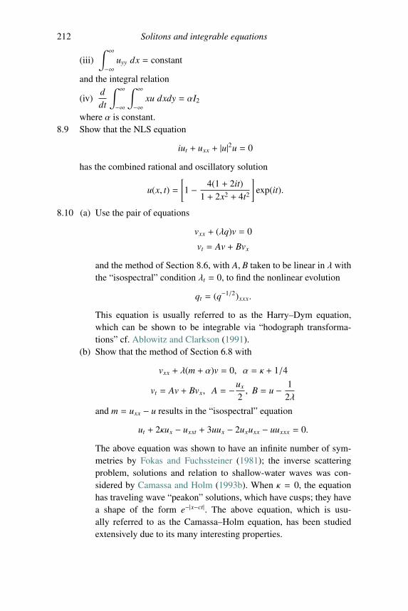
212 Solitons and integrable equations
(iii)∫ ∞
−∞uyy dx = constant
and the integral relation
(iv)ddt
∫ ∞
−∞
∫ ∞
−∞xu dxdy = αI2
where α is constant.8.9 Show that the NLS equation
iut + uxx + |u|2u = 0
has the combined rational and oscillatory solution
u(x, t) =
[1 − 4(1 + 2it)
1 + 2x2 + 4t2
]exp(it).
8.10 (a) Use the pair of equations
vxx + (λq)v = 0
vt = Av + Bvx
and the method of Section 8.6, with A, B taken to be linear in λ withthe “isospectral” condition λt = 0, to find the nonlinear evolution
qt = (q−1/2)xxx.
This equation is usually referred to as the Harry–Dym equation,which can be shown to be integrable via “hodograph transforma-tions” cf. Ablowitz and Clarkson (1991).
(b) Show that the method of Section 6.8 with
vxx + λ(m + α)v = 0, α = κ + 1/4
vt = Av + Bvx, A = −ux
2, B = u − 1
2λ
and m = uxx − u results in the “isospectral” equation
ut + 2κux − uxxt + 3uux − 2uxuxx − uuxxx = 0.
The above equation was shown to have an infinite number of sym-metries by Fokas and Fuchssteiner (1981); the inverse scatteringproblem, solutions and relation to shallow-water waves was con-sidered by Camassa and Holm (1993b). When κ = 0, the equationhas traveling wave “peakon” solutions, which have cusps; they havea shape of the form e−|x−ct|. The above equation, which is usu-ally referred to as the Camassa–Holm equation, has been studiedextensively due to its many interesting properties.
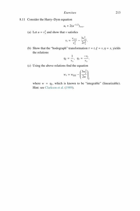
Exercises 213
8.11 Consider the Harry–Dym equation
ut + 2(u−1/2)xxx.
(a) Let u = v2x and show that v satisfies
vt =vxxx
v3x− 3v2
xx
2v4x.
(b) Show that the “hodograph” transformation τ = t, ξ = v, η = x, yieldsthe relations
ηξ =1vx, ητ =
−vt
vx.
(c) Using the above relations find the equation
wτ = wξξξ −⎛⎜⎜⎜⎜⎜⎝3w2
ξ
2w
⎞⎟⎟⎟⎟⎟⎠ξ
where w = ηξ, which is known to be “integrable” (linearizable).Hint: see Clarkson et al. (1989).
9The inverse scattering transform for the Korteweg–de
Vries (KdV) equation
We have seen in the previous chapter that the Korteweg–de Vries (KdV)equation is the result of compatibility between
vxx + (λ + u(x, t))v = 0 (9.1)
and
vt = (γ + ux)v + (4λ + 2u)vx, (9.2)
where γ is constant. More precisely, the equality of the mixed derivatives vxxt =
vtxx with λt = 0 (“isospectrality”) leads to the KdV equation
ut + 6uux + uxxx = 0. (9.3)
In the main part of this chapter we will use the above compatibility relationsin order to carry out the inverse scattering transform (IST) for the KdV equa-tion on the infinite interval. This includes a basic description of the direct andinverse problems of the time-independent Schrodinger equation and the timeevolution of the scattering data. Special soliton solutions as well as the scatter-ing data for a delta function and box potential are given. Also included are thederivation of the conserved quantities/conservation laws of the KdV equationfrom IST. Finally, as an extension, the IST associated with the second-orderscattering system and associated time (8.33)–(8.34), discussed in the previouschapter, is carried out.
For (9.1), the eigenvalues and the behavior of the eigenfunctions as |x| → ∞determine what we call the scattering data S (λ, t) at any time t, which dependsupon the potential u(x, t). The direct scattering problem maps the potential intothe scattering data. The inverse scattering problem reconstructs the potentialu(x, t) from the scattering data S (λ, t). The initial value problem for the KdVequation is analyzed as follows. At t = 0 we give initial data u(x, 0) whichwe assumes decays sufficiently rapidly at infinity. The initial data is mapped to
214
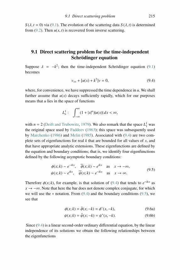
9.1 Direct scattering problem 215
S (λ, t = 0) via (9.1). The evolution of the scattering data S (λ, t) is determinedfrom (9.2). Then u(x, t) is recovered from inverse scattering.
9.1 Direct scattering problem for the time-independentSchrodinger equation
Suppose λ = −k2; then the time-independent Schrodinger equation (9.1)becomes
vxx +{u(x) + k2}v = 0, (9.4)
where, for convenience, we have suppressed the time dependence in u. We shallfurther assume that u(x) decays sufficiently rapidly, which for our purposesmeans that u lies in the space of functions
L1n :
∫ ∞
−∞(1 + |x|n)|u(x)| dx < ∞,
with n = 2 (Deift and Trubowitz, 1979). We also remark that the space L11 was
the original space used by Faddeev (1963); this space was subsequently usedby Marchenko (1986) and Melin (1985). Associated with (9.4) are two com-plete sets of eigenfunctions for real k that are bounded for all values of x, andthat have appropriate analytic extensions. These eigenfunctions are defined bythe equation and boundary conditions; that is, we identify four eigenfunctionsdefined by the following asymptotic boundary conditions:
φ(x; k) ∼ e−ikx, φ(x; k) ∼ eikx as x→ −∞,ψ(x; k) ∼ eikx, ψ(x; k) ∼ e−ikx as x→ ∞. (9.5)
Therefore φ(x; k), for example, is that solution of (9.4) that tends to e−ikx asx→ −∞. Note that here the bar does not denote complex conjugate, for whichwe will use the ∗ notation. From (9.4) and the boundary conditions (9.5), wesee that
φ(x; k) = φ(x;−k) = φ∗(x,−k), (9.6a)
ψ(x; k) = ψ(x;−k) = ψ∗(x,−k). (9.6b)
Since (9.4) is a linear second-order ordinary differential equation, by the linearindependence of its solutions we obtain the following relationships betweenthe eigenfunctions
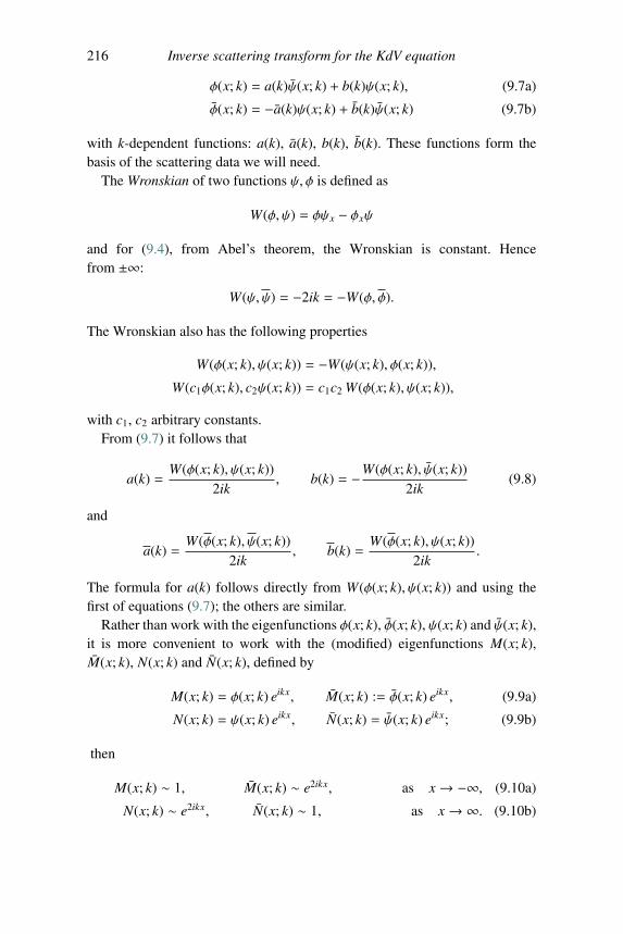
216 Inverse scattering transform for the KdV equation
φ(x; k) = a(k)ψ(x; k) + b(k)ψ(x; k), (9.7a)
φ(x; k) = −a(k)ψ(x; k) + b(k)ψ(x; k) (9.7b)
with k-dependent functions: a(k), a(k), b(k), b(k). These functions form thebasis of the scattering data we will need.
The Wronskian of two functions ψ, φ is defined as
W(φ, ψ) = φψx − φxψ
and for (9.4), from Abel’s theorem, the Wronskian is constant. Hencefrom ±∞:
W(ψ, ψ) = −2ik = −W(φ, φ).
The Wronskian also has the following properties
W(φ(x; k), ψ(x; k)) = −W(ψ(x; k), φ(x; k)),
W(c1φ(x; k), c2ψ(x; k)) = c1c2 W(φ(x; k), ψ(x; k)),
with c1, c2 arbitrary constants.From (9.7) it follows that
a(k) =W(φ(x; k), ψ(x; k))
2ik, b(k) = −W(φ(x; k), ψ(x; k))
2ik(9.8)
and
a(k) =W(φ(x; k), ψ(x; k))
2ik, b(k) =
W(φ(x; k), ψ(x; k))2ik
.
The formula for a(k) follows directly from W(φ(x; k), ψ(x; k)) and using thefirst of equations (9.7); the others are similar.
Rather than work with the eigenfunctions φ(x; k), φ(x; k), ψ(x; k) and ψ(x; k),it is more convenient to work with the (modified) eigenfunctions M(x; k),M(x; k), N(x; k) and N(x; k), defined by
M(x; k) = φ(x; k) eikx, M(x; k) := φ(x; k) eikx, (9.9a)
N(x; k) = ψ(x; k) eikx, N(x; k) = ψ(x; k) eikx; (9.9b)
then
M(x; k) ∼ 1, M(x; k) ∼ e2ikx, as x→ −∞, (9.10a)
N(x; k) ∼ e2ikx, N(x; k) ∼ 1, as x→ ∞. (9.10b)
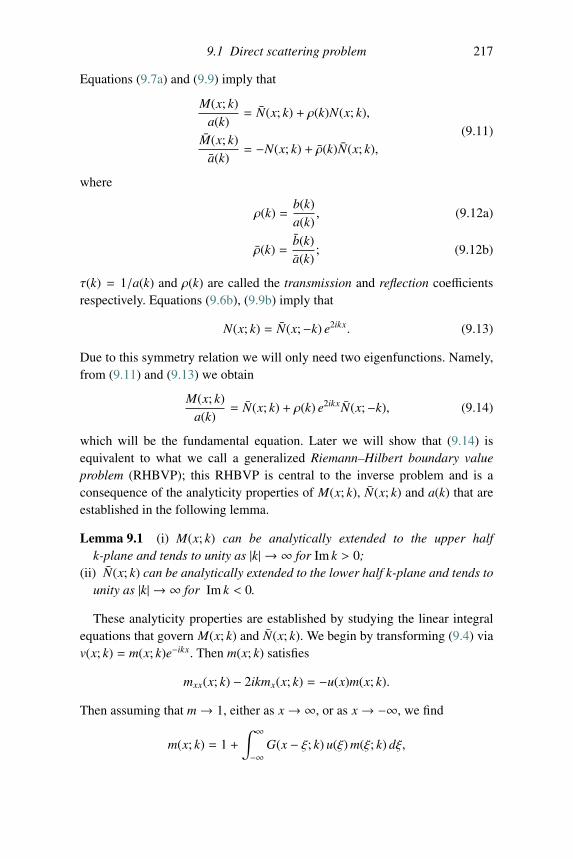
9.1 Direct scattering problem 217
Equations (9.7a) and (9.9) imply that
M(x; k)a(k)
= N(x; k) + ρ(k)N(x; k),
M(x; k)a(k)
= −N(x; k) + ρ(k)N(x; k),(9.11)
where
ρ(k) =b(k)a(k)
, (9.12a)
ρ(k) =b(k)a(k)
; (9.12b)
τ(k) = 1/a(k) and ρ(k) are called the transmission and reflection coefficientsrespectively. Equations (9.6b), (9.9b) imply that
N(x; k) = N(x;−k) e2ikx. (9.13)
Due to this symmetry relation we will only need two eigenfunctions. Namely,from (9.11) and (9.13) we obtain
M(x; k)a(k)
= N(x; k) + ρ(k) e2ikxN(x;−k), (9.14)
which will be the fundamental equation. Later we will show that (9.14) isequivalent to what we call a generalized Riemann–Hilbert boundary valueproblem (RHBVP); this RHBVP is central to the inverse problem and is aconsequence of the analyticity properties of M(x; k), N(x; k) and a(k) that areestablished in the following lemma.
Lemma 9.1 (i) M(x; k) can be analytically extended to the upper halfk-plane and tends to unity as |k| → ∞ for Im k > 0;
(ii) N(x; k) can be analytically extended to the lower half k-plane and tends tounity as |k| → ∞ for Im k < 0.
These analyticity properties are established by studying the linear integralequations that govern M(x; k) and N(x; k). We begin by transforming (9.4) viav(x; k) = m(x; k)e−ikx. Then m(x; k) satisfies
mxx(x; k) − 2ikmx(x; k) = −u(x)m(x; k).
Then assuming that m→ 1, either as x→ ∞, or as x→ −∞, we find
m(x; k) = 1 +∫ ∞
−∞G(x − ξ; k) u(ξ) m(ξ; k) dξ,
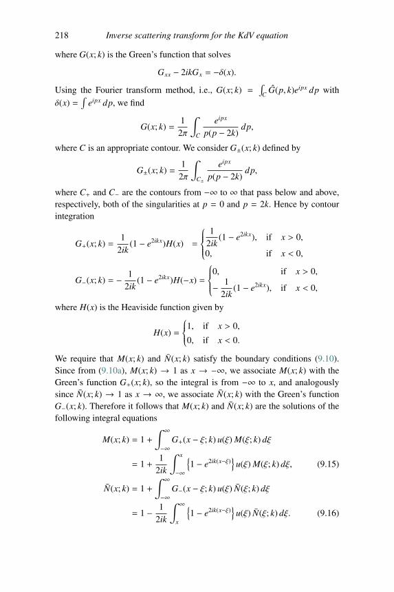
218 Inverse scattering transform for the KdV equation
where G(x; k) is the Green’s function that solves
Gxx − 2ikGx = −δ(x).
Using the Fourier transform method, i.e., G(x; k) =∫
CG(p, k)eipx dp with
δ(x) =∫
eipx dp, we find
G(x; k) =1
2π
∫C
eipx
p(p − 2k)dp,
where C is an appropriate contour. We consider G±(x; k) defined by
G±(x; k) =1
2π
∫C±
eipx
p(p − 2k)dp,
where C+ and C− are the contours from −∞ to ∞ that pass below and above,respectively, both of the singularities at p = 0 and p = 2k. Hence by contourintegration
G+(x; k) =1
2ik(1 − e2ikx)H(x) =
⎧⎪⎪⎪⎨⎪⎪⎪⎩1
2ik(1 − e2ikx), if x > 0,
0, if x < 0,
G−(x; k) = − 12ik
(1 − e2ikx)H(−x) =
⎧⎪⎪⎪⎨⎪⎪⎪⎩0, if x > 0,
− 12ik
(1 − e2ikx), if x < 0,
where H(x) is the Heaviside function given by
H(x) =
⎧⎪⎪⎨⎪⎪⎩1, if x > 0,
0, if x < 0.
We require that M(x; k) and N(x; k) satisfy the boundary conditions (9.10).Since from (9.10a), M(x; k) → 1 as x → −∞, we associate M(x; k) with theGreen’s function G+(x; k), so the integral is from −∞ to x, and analogouslysince N(x; k) → 1 as x → ∞, we associate N(x; k) with the Green’s functionG−(x; k). Therefore it follows that M(x; k) and N(x; k) are the solutions of thefollowing integral equations
M(x; k) = 1 +∫ ∞
−∞G+(x − ξ; k) u(ξ) M(ξ; k) dξ
= 1 +1
2ik
∫ x
−∞
{1 − e2ik(x−ξ)} u(ξ) M(ξ; k) dξ, (9.15)
N(x; k) = 1 +∫ ∞
−∞G−(x − ξ; k) u(ξ) N(ξ; k) dξ
= 1 − 12ik
∫ ∞
x
{1 − e2ik(x−ξ)} u(ξ) N(ξ; k) dξ. (9.16)
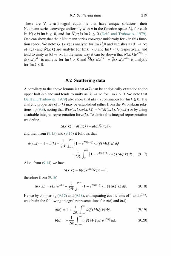
9.2 Scattering data 219
These are Volterra integral equations that have unique solutions; theirNeumann series converge uniformly with u in the function space L1
2, for eachk: M(x; k) Im k ≥ 0, and for N(x; k) Im k ≤ 0 (Deift and Trubowitz, 1979).One can show that their Neumann series converge uniformly for u in this func-tion space. We note: G±(x; k) is analytic for Im k >
<0 and vanishes as |k| → ∞;
M(x; k) and N(x; k) are analytic for Im k > 0 and Im k < 0 respectively, andtend to unity as |k| → ∞. In the same way it can be shown that N(x; k)e−2ikx =
ψ(x; k)eikx is analytic for Im k > 0 and M(x; k)e2ikx = ψ(x; k)e−ikx is analyticfor Im k < 0.
9.2 Scattering data
A corollary to the above lemma is that a(k) can be analytically extended to theupper half k-plane and tends to unity as |k| → ∞ for Im k > 0. We note thatDeift and Trubowitz (1979) also show that a(k) is continuous for Im k ≥ 0. Theanalytic properties of a(k) may be established either from the Wronskian rela-tionship (9.8), noting that W(φ(x; k), ψ(x; k)) = W(M(x; k),N(x; k)) or by usinga suitable integral representation for a(k). To derive this integral representationwe define
Δ(x; k) = M(x; k) − a(k)N(x; k),
and then from (9.15) and (9.16) it follows that
Δ(x; k) = 1 − a(k) +1
2ik
∫ ∞
−∞
{1 − e2ik(x−ξ)} u(ξ) M(ξ; k) dξ
− 12ik
∫ ∞
x
{1 − e2ik(x−ξ)} u(ξ)Δ(ξ; k) dξ. (9.17)
Also, from (9.14) we have
Δ(x; k) = b(k) e2ikxN(x;−k);
therefore from (9.16)
Δ(x; k) = b(k) e2ikx − 12ik
∫ ∞
x
{1 − e2ik(x−ξ)} u(ξ)Δ(ξ; k) dξ. (9.18)
Hence by comparing (9.17) and (9.18), and equating coefficients of 1 and e2ikx,we obtain the following integral representations for a(k) and b(k):
a(k) = 1 +1
2ik
∫ ∞
−∞u(ξ) M(ξ; k) dξ, (9.19)
b(k) = − 12ik
∫ ∞
−∞u(ξ) M(ξ; k) e−2ikξ dξ. (9.20)
220 Inverse scattering transform for the KdV equation
From these integral representations it follows that a(k) is analytic for Im k > 0,and tends to unity as |k| → ∞, while b(k) cannot, in general, be continuedanalytically off the real k-axis. Furthermore, since M(x; k) → 1 as κ → ∞,then it follows from (9.19) that a(k) → 1 as κ (for Im k > 0). Similarly it canbe shown that a(k) can be analytically extended to the lower half k-plane andtends to unity as |k| → ∞ for Im k < 0.
The functions a(k), a(k), b(k), b(k) satisfy the condition
a(k)a(k) + b(k)b(k) = −1. (9.21)
This follows from the Wronskian and its relations:
W(φ(x; k), φ(x; k)) = W(a(k)ψ(x; k) + b(k)ψ(x; k),
− a(k)ψ(x; k) + b(k)ψ(x; k))
={a(k)a(k) + b(k)b(k)
}W(ψ(x; k), ψ(x; k)),
with W(φ(x; k), φ(x; k)) = 2ik = −W(ψ(x; k), ψ(x; k)). From the definitions ofthe reflection and transmission coefficients, we see that τ(k) and ρ(k) satisfy
|ρ(k)|2 + |τ(k)|2 = 1.
Using (9.4)–(9.7) and their complex conjugates we have the symmetry condi-tions
a(k) = −a(−k) = −a∗(k∗),
b(k) = b(−k) = b∗(k∗),(9.22)
where a∗(k∗), b∗(k∗) are the complex conjugates of a(k), b(k), respectively.The zeros of a(k) play an important role in the inverse problem; they are
poles in the generalized Riemann–Hilbert problem obtained from (9.14). Wenote the following: the function a(k) can have a finite number of zeros atk1, k2, . . . , kN , where k j = iκ j, κ j ∈ R, j = 1, 2, . . . ,N# (i.e., they all lie onthe imaginary axis), in the upper half k-plane.
First we see that from equations (9.21), (9.22) that
|a(k)|2 − |b(k)|2 = 1,
for k ∈ R; hence a(k) � 0 for k ∈ R. Recall that φ(x; k), ψ(x; k) and ψ(x; k) aresolutions of the Schrodinger equation (9.4) satisfying the boundary conditions
φ(x; k) ∼ e−ikx, as x→ −∞,ψ(x; k) ∼ eikx, as x→ ∞,ψ(x; k) ∼ e−ikx, as x→ ∞,
(9.23)
9.2 Scattering data 221
together with the relationship
φ(x; k) = a(k)ψ(x; k) + b(k)ψ(x; k). (9.24)
From (9.8) it follows that
W(φ(x; k), ψ(x; k)) = φ(x; k)ψx(x; k) − φx(x; k)ψ(x; k) = 2ika(k).
Thus at any zero k j of a(k), we have that φ(x; k), ψ(x; k) are linearly indepen-dent. In order to have a rapidly decaying state; i.e., a bound state where φ(x; k j)is in L2(R), we must have that Im k j > 0.
The eigenfunction φ(x; k) and its complex conjugate φ∗(x; k∗) satisfy theequations
φxx +{u(x) + k2
}φ = 0,
φ∗xx +{u(x) + (k∗)2
}φ∗ = 0,
(9.25)
respectively. Hence
∂
∂xW(φ, φ∗) +
[(k∗)2 − k2
]φφ∗ = 0,
which implies [(k∗)2 − k2
] ∫ ∞
−∞|φ(x; k)|2 dx = 0 (9.26)
since φ and its derivatives vanish as x→ ±∞. Further, calling k j = ξ j + η j, we
see by taking the real part of (9.26):(k∗j)2 − k2
j = −2ξ jη j = 0, any zero of amust be purely imaginary; i.e., Re k j = ξ j = 0.
To show that a(k) has only a finite number of zeros, we note that a → 1 as|k| → ∞; furthermore, it is shown by Deift and Trubowitz (1979) that a(k) iscontinuous for Im k ≥ 0. Hence there can be no cluster points of zeros of a(k)either in the upper half k-plane or on the real k-axis and so necessarily a(k) canpossess only a finite number of zeros.
We can also show that the zeros of a(k) are simple by studying the derivativeda/dk with respect to k: but we will not do this here (see Deift and Trubowitz,1979).
Hence, as long as u ∈ L12, M(x; k)/a(k) is a meromorphic function in the
upper half k-plane with a finite number of simple poles at k = iκ1, iκ2, . . . , iκN#.
Then set
M(x; k)a(k)
= μ+(x; k) +N#∑j=1
Aj(x)
k − iκ j, (9.27)
222 Inverse scattering transform for the KdV equation
where μ+(x; k) is analytic in the upper half k-plane. Integrating (9.27) aroundiκ j and using (9.14) and the fact that at a discrete eigenvalue M,N areproportional, M(x; iκ j) = b jN(x; iκ j), shows that
Aj(x) = C jN(x;−iκ j) exp(−2κ j x),
where C j = b j/a′j. Hence from (9.14) we obtain
μ+(x; k) = N(x; k) −N#∑j=1
C j
k − iκ jexp(−2κ j x)N(x;−iκ j)
+ ρ(k) exp(2ikx)N(x;−k). (9.28)
Furthermore, μ+(x; k)→ 1 as κ → 1, for Im k > 0.
9.3 The inverse problem
Equation (9.28) defines a Riemann–Hilbert problem (cf. Ablowitz and Fokas,2003) in terms of the scattering data S (λ) =
{(κ j,C j)N#
j=1, ρ(k), a(k)}. We will
use the following.Consider the P± projection operator defined by
(P± f )(k) =1
2πi
∫ ∞
−∞f (ζ)
ζ − (k ± i0)dζ = lim
ε↓0
{1
2πi
∫ ∞
−∞f (ζ)
ζ − (k ± iε)dζ
}.
(9.29)Suppose that f±(k) is analytic in the upper/lower half k-plane and f±(k)→ 0 as|k| → ∞ (for Im k >
<0). Then
(P± f∓)(k) = 0,
(P± f±)(k) = ± f±(k).
These results follow from contour integration.To explain the ideas most easily, we first assume that there are no poles;
that is, a(k) � 0. Then (9.28) reduces to (9.14), because M(x; k)/a(k) = μ+.In (9.14) unity from both N and M/a and operating on (9.14) with P− andusing the analytic properties of M, N and a yields
P−[(
M(x; k)a(k)
− 1
)]= P−
[(N(x; k) − 1) + ρ(k)e2ikxN(x;−k)
].
This implies
0 =(N(x; k) − 1
)+
12πi
∫ ∞
−∞ρ(ζ) e2iζx N(x;−ζ)
ζ − (k − i0)dζ.
9.3 The inverse problem 223
Then employing the symmetry: N(x; k) = e2ikxN(x;−k) and N(x;−k) =e−2ikxN(x; k), it follows that
N(x; k) = 1 +1
2πi
∫ ∞
−∞ρ(ζ) N(x; ζ)ζ − (k − i0)
dζ,
N(x; k) = e2ikx
{1 +
12πi
∫ ∞
−∞ρ(ζ) N(x; ζ)ζ + k + i0
dζ
}.
(9.30)
As k → ∞, equation (9.30a) shows that
N(x; k) ∼ 1 − 12πi
1k
∫ ∞
−∞ρ(ζ) N(x; ζ) dζ, (9.31)
From the integral equation for N(x; k), equation (9.16), using the Riemann–Lebesgue lemma, we also see that as κ → ∞
N(x; k) ∼ 1 − 12ik
∫ ∞
xu(ξ) dξ. (9.32)
Therefore, by comparing (9.31) and (9.32), it follows that the potential can bereconstructed from
u(x) = − ∂∂x
{1π
∫ ∞
−∞ρ(ζ) N(x; ζ) dζ
}. (9.33)
For the case when a(k) has zeros, one can extend the above result. Supposethat
a(iκ j) = 0, κ j ∈ R, j = 1, 2, . . . ,N#;
then define
Mj(x) = M(x; iκ j),
Nj(x) = exp(−2κ j x)N(x;−iκ j),
for j = 1, 2, . . . ,N#. In (9.28) subtracting unity from both μ+(x, k) andN(x; k) and applying the P− projection operator (9.29) to (9.28), recallingthat N(x; k) = e2ikxN(x;−k) and carrying out the contour integration of simplepoles, we find the following integral equations
N(x; k) = e2ikx
⎧⎪⎪⎪⎨⎪⎪⎪⎩1 −N#∑j=1
C jNj(x)
k + iκ j+
12πi
∫ ∞
−∞ρ(ζ) N(x; ζ)ζ + k + i0
dζ
⎫⎪⎪⎪⎬⎪⎪⎪⎭ , (9.34)
Np(x) = exp(−2κpx)
⎧⎪⎪⎪⎨⎪⎪⎪⎩1 + iN#∑j=1
C jNj(x)
κp + κ j+
12πi
∫ ∞
−∞ρ(ζ) N(x; ζ)ζ + iκp
dζ
⎫⎪⎪⎪⎬⎪⎪⎪⎭ ,(9.35)
224 Inverse scattering transform for the KdV equation
for p = 1, 2, . . .N#, with the potential reconstructed from [following the samemethod that led to (9.33)]
u(x) =∂
∂x
⎧⎪⎪⎪⎨⎪⎪⎪⎩2iN#∑j=1
C jNj(x) − 1π
∫ ∞
−∞ρ(k) N(x; k) dk
⎫⎪⎪⎪⎬⎪⎪⎪⎭ . (9.36)
Existence and uniqueness of solutions to equations such as (9.34)–(9.36) isgiven by Beals et al. (1988). We also note that the above integral equa-tions (9.34) and (9.35) can be transformed to Gel’fand–Levitan–Marchenkointegral equations, see Section 9.5 below, from which one can also deduce theexistence and uniqueness of solutions (cf. Marchenko, 1986).
9.4 The time dependence of the scattering data
In this section we will find out how the scattering data evolves. The time evo-lution of the scattering data may be obtained by analyzing the asymptoticbehavior of the associated time evolution operator, which as we have seenearlier for the KdV equation is
vt = (ux + γ)v + (4k2 − 2u)vx,
with γ a constant. If we let v = φ(x; k) and make the transformation
φ(x, t; k) = M(x, t; k) e−ikx,
M then satisfies
Mt = (γ − 4ik3 + ux + 2iku)M + (4k2 − 2u)Mx. (9.37)
Recall that from (9.11)
M(x, t; k) = a(k, t)N(x, t; k) + b(k, t)N(x, t;−k),
where ρ(k, t) = b(k, t)/a(k, t). From (9.10) the asymptotic behavior of M(x, t; k)is given by
M(x, t; k)→ 1, as x→ −∞,M(x, t; k)→ a(k, t) + b(k, t) e2ikx, as x→ ∞.
By using using the fact that u→ 0 rapidly as x→ ±∞ and the above equationit follows from (9.37) that
γ − 4ik3 = 0, x→ −∞at + bt e2ikx = 8ik3b e2ikx, x→ +∞,
9.5 The Gel’fand–Levitan–Marchenko integral equation 225
and by equating coefficients of e0, e2ikx we find
at = 0, bt = 8ik3b. (9.38)
Solving (9.38) yields
a(k, t) = a(k, 0), b(k, t) = b(k, 0) exp(8ik3t), (9.39)
and so
ρ(k, t) ≡ b(k, t)a(k, t)
= ρ(k, 0) exp(8ik3t).
Since a(k, t) does not evolve in time, the discrete eigenvalues, which are thezeros of a(k) that are finite in number, simple, and lie on the imaginary axis,satisfy
k j = iκ j = constant, j = 1, 2, . . . ,N#.
Since the eigenvalues are constant in time, we say this is an “isospectral flow”.Similarly we find that the time dependence of the C j(t) is given by
C j(t) = C j(0) exp(8ik3
j t)= C j(0) exp
(8κ3
j t). (9.40)
9.5 The Gel’fand–Levitan–Marchenko integral equation
The Gel’fand–Levitan–Marchenko integral equation may be derived from theabove formulation. We assume a “triangular” kernel K(x, s; t) (see also below)such that
N(x, t; k) = e2ikx
{1 +∫ ∞
xK(x, s; t) eik(s−x) ds
}, (9.41)
where K(x, s; t) is assumed to decay rapidly as x and s → ∞. Substitut-ing (9.41) into (9.34)–(9.35) and taking the Fourier transform, i.e., operatingwith
12π
∫ ∞
−∞dk eik(x−y), for y > x
we find that
K(x, y; t) + F(x + y; t) +∫ ∞
xK(x, s; t) F(s + y; t) ds = 0, y > x, (9.42)
where
F(x; t) =N#∑j=1
−iC j(0) exp(8κ3
j t − κ j x)+
12π
∫ ∞
−∞ρ(k, t) eikx dk. (9.43)
226 Inverse scattering transform for the KdV equation
Substituting (9.41) into (9.36) we have
u(x, t) = 2∂
∂xK(x, x; t). (9.44)
Thus we have shown that the Gel’fand–Levitan–Marchenko equation (9.42)arises from the integral equations that result from the Riemann–Hilbertboundary value problem.
We can also show that K(x, s, t) satisfies a PDE in x, s; i.e., it is independentof k. Using (9.41), then from
N = eikxψ
we have
ψ = eikx +
∫ ∞
xK(x, s, t)eiks ds.
We wish to use this in
ψxx + (u(x, t) + k2)ψ = 0 (9.45)
so we calculate
ψx = ikeikx − K(x, x, t)eikx +
∫ ∞
xKx(x, s, t)eiks ds
and
ψxx = −k2eikx − ddx
K(x, x, t)eikx
− ikK(x, x, t)eikx +
∫ ∞
xKxx(x, s, t)eiks ds − Kx(x, x, t)eikx.
Part of the third term in (9.45) becomes after integrating by parts
k2∫ ∞
xK(x, s, t)eiks ds = −
∫ ∞
xK(x, s, t)
∂2
∂s2eiks ds
= K(x, x, t)ikeikx +
∫ ∞
x
∂K∂s
∂
∂seiks ds
= −ikK(x, x, t)eikx − ∂K∂s
(x, x, t)eikx
−∫ ∞
x
∂2K∂s2
eiks ds.
9.6 Outline of the inverse scattering transform for the KdV equation 227
Then using all of the above in (9.45) gives
− ddx
K(x, x, t)eikx +
∫ ∞
x
∂2
∂x2K(x, s, t)eiks ds − ∂
∂xK(x, s = x, t)eikx
+ ueikx +
∫ ∞
xu(x)K(x, s, t)eiks ds − ∂K
∂s(x, x, t)eikx
−∫ ∞
x
∂2K∂s2
(x, s, t)eiks ds = 0
which in turn leads to∫ ∞
x[(Kxx − Kss) − uK(x, s, t)]eikx ds
+
⎡⎢⎢⎢⎢⎢⎢⎢⎢⎢⎢⎢⎢⎢⎢⎢⎢⎣−ddx
K(x, x, t)− ∂∂x
K(x, s = x, t) − ∂
∂sK(x, x, t)︸������������������������������������︷︷������������������������������������︸
− ddx K(x,x,t)
+u
⎤⎥⎥⎥⎥⎥⎥⎥⎥⎥⎥⎥⎥⎥⎥⎥⎥⎦ eikx = 0
which for arbitrary kernels leads to
(Kxx − Kss) − u(x)K(x, s, t) = 0, u(x, t) = 2ddx
K(x, x, t), s > x
where t is a parameter and K(x, s; t) decays rapidly as x and s → ∞. SinceK satisfies the above system, which is a well-posed Goursat problem (Garabe-dian, 1984), this indicates the solution exists and is unique. Hence, this showsthat K(x, y, t) satisfies a wave-like PDE independent of k.
9.6 Outline of the inverse scattering transformfor the KdV equation
We have seen that associated with the KdV equation (9.3) is a linear scat-tering problem (9.1) and time-dependent equation (9.2). These equations arecompatible if the eigenvalues λ → iκ j, j = 1, . . .N#, are time-independent, orisospectral, i.e. κ j,t = 0.
The direct scattering problem maps a decaying potential (u ∈ L12) into the
scattering data. The inverse scattering problem reconstructs the potential fromthe scattering data. The time evolution equation tells us how the scattering dataevolves.
The solution of the KdV equation (9.3) proceeds as follows: at time t = 0,given u(x, 0) we solve the direct scattering problem. This involves solving theintegral equations (9.15)–(9.16) and using these results to obtain the scatteringdata (9.19)–(9.20). The scattering data needed are:
228 Inverse scattering transform for the KdV equation
S (k, 0) =
({κ j,C j(0)}N#
j=1, ρ(k, 0) ≡ b(k, 0)a(k, 0)
),
where κ j, j = 1, 2, . . . ,N#, are the locations of the zeros of a(k, 0) and C j(0),j = 1, 2, . . . ,N#, are often called the associated “normalization constants” thatwere also defined above.
Next we determine the time evolution of the scattering data using equations(9.39)–(9.40). This yields the scattering data at any time t:
S (k, t) =
({κ j,C j(t)}N#
j=1, ρ(k, t) ≡ b(k, t)a(k, t)
).
For the inverse problem, at time t, we solve either the integral equations forN(x, t) and reconstruct u(x, t) via (9.34)–(9.36) or solve the Gel’fand–Levitan–Marchenko equations for K(x, y, t) and reconstruct u(x, t) via (9.42)–(9.44).
This method is conceptually analogous to the Fourier transform method forsolving linear equations (discussed in Chapter 2), except however the stepof solving the inverse scattering problem requires one to solve a linear inte-gral equation (i.e., a Riemann–Hilbert boundary value problem) that addscomplications. Schematically the solution is given by
u(x, 0)direct scattering−−−−−−−−−−−→ S (k, 0) =
({κn,C j(0)}N#
j=1, ρ(k, 0), a(k, 0))
⏐⏐⏐⏐⏐*t: time evolution
u(x, t)inverse scattering←−−−−−−−−−−−− S (k, t) =
({κn,C j(t)}N#
j=1, ρ(k, t), a(k, t))
In the analogy of IST to the Fourier transform method for linear partial dif-ferential equations, the direct scattering problem and the scattering data playthe role of the Fourier transform and the inverse scattering problem the inverseFourier transform.
9.7 Soliton solutions of the KdV equation
In this section we will describe how the inverse scattering method can be usedto find soliton solutions of the Korteweg–de Vries equation (9.3).
9.7.1 The Riemann–Hilbert method
Pure soliton solutions may be obtained from (9.34)–(9.36) in the case whenρ(k, t) = 0 on the real k-axis. This is usually called a reflectionless potential.We assume a special form for ρ(k; t), namely
9.7 Soliton solutions of the KdV equation 229
ρ(k; t) =
⎧⎪⎪⎪⎪⎪⎪⎨⎪⎪⎪⎪⎪⎪⎩0, if k real,N#∑j=1
C j(0)
k − iκ jexp(8κ3
j t), if Im k > 0.
Then we obtain a linear algebraic system for the Nj(x, t)
Nj(x, t) −N#∑
m=1
iCm(0)κm + κ j
exp(−2κmx + 8κ3
mt)
Nm(x, t) = exp(−2κ j x), (9.46)
where j = 1, 2, . . . , N, Nj(x, t) := N(x; k = iκ j; t), and the potential u(x, t) isgiven by
u(x, t) = 2∂
∂x
⎧⎪⎪⎪⎨⎪⎪⎪⎩N#∑j=1
exp(8κ3
j t)
iC j(0)Nj(x, t)
⎫⎪⎪⎪⎬⎪⎪⎪⎭ .In the case of the one-soliton solution, the number of eigenvalues is N# = 1and (9.46) reduces to
N1(x, t) − iC1(0)2κ1
exp(−2κ1x + 8κ3
1t)
N1(x, t) = exp(−2κ1x),
and so
N1(x, t) =2κ1 exp(−2κ1x)
2κ1 − iC1(0) exp(−2κ1x + 8κ3
1t) .
Therefore
u(x, t) = 2∂
∂x
{exp(8κ3
1t)
iC1(0)N1(x, t)}
= 2∂
∂x
⎧⎪⎪⎪⎨⎪⎪⎪⎩ 2κ1iC1(0) exp(−2κ1x + 8κ3
1t)
2κ1 − iC1(0) exp(−2κ1x + 8κ3
1t)⎫⎪⎪⎪⎬⎪⎪⎪⎭
= 2∂
∂x
⎧⎪⎪⎪⎨⎪⎪⎪⎩ 2κ1iC1(0)
2κ1 exp(2κ1x − 8κ3
1t)− iC1(0)
⎫⎪⎪⎪⎬⎪⎪⎪⎭=
8κ21[
exp(κ1x − κ3
1t − κ1x1
)+ exp
(−κ1x + κ3
1t + κ1x1
)]2where we define −iC1(0) = 2κ1 exp(2κ1x1); hence we obtain the one-solitonsolution
230 Inverse scattering transform for the KdV equation
u(x, t) = 2κ21 sech2
{κ1
(x − 4κ2
1t − x1
)}.
In the case of the two-solution solution, we have to first solve a linear system
N1(x, t) +2∑
j=1
C j(0)
κ j + κ1exp(−2κ j x + 8κ3
j t)
Nj(x, t) = exp(−2κ1x),
N2(x, t) +2∑
j=1
C j(0)
κ j + κ2exp(−2κ j x + 8κ3
j t)
Nj(x, t) = exp(−2κ2x),
for N1(x, t) and N2(x, t). After some algebra, the two-soliton solution of theKdV equation is found to be
u(x, t) =4(κ2
2 − κ21
) [(κ2
2 − κ21
)+ κ2
1 cosh(2κ2ξ2) + κ22 cosh(2κ1ξ1)
][(κ2 − κ1) cosh(κ1ξ1 + κ2ξ2) + (κ2 + κ1) cosh(κ2ξ2 − κ1ξ1)
]2 ,where ξi = x − 4κ2
i t − xi, and Ci(0) = 2κi exp(2κi xi), for i = 1, 2.
9.7.2 Gel’fand–Levitan–Marchenko approach
Again we suppose that the potential u(x, 0) is reflectionless, ρ(k, 0) = 0, andthe time-independent Schrodinger equation (9.4) has N# discrete eigenvalueskn = iκn, n = 1, 2, . . . ,N#, such that 0 < κ1 < κ2 < · · · < κN# . To connect withthe standard approach, in the kernel F(x, t) in the Gel’fand–Levitan–Marc-henko equation (9.42)–(9.43) we take −iCn = c2
n. In this way the associatedeigenfunctions ψn(x), n = 1, 2, . . . ,N#, satisfy the normalization condition∫ ∞
−∞ψ2
n(x) dx = 1,
and the asymptotic limit as x → +∞, limx→+∞ ψn(x) exp(κnx) = cn(0), wherec j(0) are called the Gel’fand–Levitan–Marchenko normalization constants;and cn(t) = cn(0) exp
(4κ3
nt).
Then this is solvable by a separation of variables (cf. Kay and Moses, 1956;Gardner et al., 1974). Here we take
F(x; t) =N#∑
n=1
c2n(0) exp
(8κ3
nt − κnx),
9.7 Soliton solutions of the KdV equation 231
and so the Gel’fand–Levitan–Marchenko equation becomes
K(x, y; t) +N#∑
n=1
c2n(t) exp{−κn(x + y)}
+
∫ ∞
xK(x, s; t)
N∑n=1
c2n(t) exp{−κn(s + y)} ds = 0. (9.47)
Now we seek a solution of this equation in the form
K(x, y; t) =N#∑
n=1
Ln(x, t) exp(−κny),
and then the integral equation (9.47) reduces to a linear algebraic system
Ln(x, t) +N#∑
m=1
c2n(t)
κm + κnexp{−(κm + κn)x}Lm(x, t) + c2
n(t) exp(−κnx) = 0,
for n = 1, 2, . . . ,N#. We can, in principle, solve this linear system. We will goa little further.
If we let Ln(x, t) = −cn(t)wn(x, t), for n = 1, 2, . . . ,N#, this yields a systemthat can be written in the convenient form
(I + B)w = f, (9.48)
where w = (w1,w2, . . . ,wN# ), f = ( f1, f2, . . . , fN# ) with fn(x, t) =
cn(t) exp(−κnx) for n = 1, 2, . . . ,N#, I is the N# × N# identity matrix and Bis a symmetric, N# × N# matrix with entries
Bmn(x, t) =cm(t)cn(t)κm + κn
exp{−(κm + κn)x}, m, n = 1, 2, . . . ,N#.
The system (9.48) has a unique solution when B is positive definite. If weconsider the quadratic form
vTBv =N#∑
m=1
N#∑n=1
cm(t)cn(t)vmvn
κm + κnexp{−(κm + κn)x}
=
∫ ∞
x
⎡⎢⎢⎢⎢⎢⎢⎣ N#∑n=1
cn(t)vn exp(−κny)
⎤⎥⎥⎥⎥⎥⎥⎦2
dy,
where v = (v1, v2, . . . , vN# ), which is positive and vanishes only if v = 0; thenB is positive definite.
232 Inverse scattering transform for the KdV equation
If in the kernel, F(x, t), of the Gel’fand–Levitan–Marchenko equation(9.47), we take N# = 1 and define c2
1(0) = 2κ1 exp (2κ1x1), then we find theone-soliton solution
u(x, t) = 2κ21 sech2
{κ1
(x − 4κ2
1t − x1
)},
which is the same as derived from the RHBVP approach. The general N#-soliton case was analyzed in detail by Gardner et al. (1974).
9.8 Special initial potentials
In the previous sections we obtained pure soliton solutions for the KdV equa-tion corresponding to reflectionless potentials. However, more general choicesof the initial data u(x, 0) give rise to non-zero reflection coefficients; unfortu-nately, in this case it generally is not possible to solve the inverse equationsin explicit form. However, long-time asymptotic information can be obtained(Ablowitz and Segur, 1979; Deift and Zhou, 1992; Deift et al., 1994).
9.8.1 Delta function initial profile
As an example consider the delta function initial profile given by
u(x; 0) = Qδ(x),
where Q is constant and δ(x) is the Dirac delta function. We use theSchrodinger equation
vxx + (k2 + u(x, 0))v = 0
with the scattering definitions given by (9.23)–(9.24). So
φ(x; k) = e−ikx, for x < 0,
ψ(x; k) = eikx, for x > 0, and
ψ(x; k) = e−ikx, for x > 0.
Then requiring the function v to be continuous and satisfy the jump condition
[vx]0+0− + Qv(0) = 0,
and letting v(x, k) = φ(x; k) yields the following equations
a(k, 0) + b(k, 0) = 1
a(k, 0)(−ik) + b(k, 0)(ik) = −Q − ik.
Hence
a(k, 0) =2ik + Q
2ik= a(k, t) =
1τ(k, t)
, b(k, 0) =−Q2ik
, ρ(k, t) =−Q
2ik + Q.
9.8 Special initial potentials 233
Thus in this case, when Q > 0, there is a single discrete eigenvalue λ = −κ21,
where κ1 = Q/2. The reflection coefficient is non-zero and given by
ρ(k, 0) =−κ1
κ1 + ik,
and similarly we find C1(0) = iκ1. The time evolution follows as above; it isgiven by
κ1 = constant, C1(t) = iκ1 exp(8κ3
1t), ρ(k, t) =
−κ1 exp(8ik3t)κ1 + ik
.
9.8.2 Box initial profile
Here we outline how to find the data associated with a box profile at t = 0:
u(x, 0) =
⎧⎪⎪⎨⎪⎪⎩H2, |x| < L/2
0, |x| > L/2
where H, L > 0 are constant. Again, we use the Schrodinger equation
vxx + (k2 + u(x, 0))v = 0
with the scattering functions/coefficients satisfying (9.23)–(9.24).Since this is a linear, constant coefficient, second-order differential equation
we have
v(x) =
⎧⎪⎪⎪⎪⎪⎨⎪⎪⎪⎪⎪⎩Aeikx + Be−ikx, x < −L/2
Ceiλx + De−iλx, |x| < L/2
Eeikx + Fe−ikx, x > L/2
where λ ≡ √H2 + k2 and so
v′(x) =
⎧⎪⎪⎪⎪⎪⎨⎪⎪⎪⎪⎪⎩Aikeikx − Bike−ikx, x < −L/2
Ciλeiλx − Diλe−iλx, |x| < L/2
Eikeikx − Fike−ikx, x > L/2.
Let us first consider the case when A = 0 and B = 1; then, requiring v andvx to be continuous at x = ±L/2 implies
eikL/2 = Ce−iλL/2 + DeiλL/2,
−ikeikL/2 = Ciλe−iλL/2 − DiλeiλL/2,
EeikL/2 + Fe−ikL/2 = CeiλL/2 + De−iλL/2,
EikeikL/2 − Fike−ikL/2 = CiλeiλL/2 − Diλe−iλL/2.
234 Inverse scattering transform for the KdV equation
Solving for the constants C,D, E, F gives
C =λ − k
2λei(k+λ)L/2,
D =λ + k
2λei(k−λ)L/2,
E = −k2 − λ2
4kλ
(eiLλ − e−iLλ
),
F = −eiL(k−λ)
4kλ
{(k − λ)2e2iLλ − (k + λ)2
}.
We define the function φ ∼ e−ikx as x→ −∞, so
φ(x) ≡
⎧⎪⎪⎪⎪⎪⎪⎪⎪⎪⎨⎪⎪⎪⎪⎪⎪⎪⎪⎪⎩e−ikx, x < −L/2
eikL/2{cos [λ(L/2 + x)] − ik
λsin [λ(L/2 + x)]
}, |x| < L/2
e−ik(x−L) cos (λL)
− i sin(λL)2kλ
[e−ik(x−L)(λ2 + k2) − eikx(λ2 − k2)
], x > L/2.
Now, let us consider the case when A = 1 and B = 0; then solving for C, D,E, F by enforcing continuity of v and vx at x = ±L/2 gives
C =λ + k
2λei(k−λ)L/2,
D =λ − k
2λei(k+λ)L/2,
E = e−ikL
{cos (λL) + i
λ2 + k2
2kλsin (λL)
},
F = iλ2 − k2
2kλsin (λL) .
We then define φ ∼ e−ikx as x→ −∞ and find
φ(x) ≡
⎧⎪⎪⎪⎪⎪⎪⎪⎪⎪⎨⎪⎪⎪⎪⎪⎪⎪⎪⎪⎩eikx, x < −L/2
e−ikL/2{cos [λ(L/2 + x)] + ik
λsin [λ(L/2 + x)]
}, |x| < L/2
eik(x−L) cos (λL)
+i sin(λL)
2kλ
[eik(x−L)(λ2 + k2) − e−ikx(λ2 − k2)
], x > L/2.
Recall the eigenfunctions ψ, ψ have the asymptotic boundary conditions: ψ ∼eikx as x→ ∞ and ψ ∼ e−ikx as x→ ∞; we write:
φ(x) = a(k)ψ(x) + b(k)ψ(x) ∼ a(k)e−ikx + b(k)eikx,
9.9 Conserved quantities and conservation laws 235
as x→ ∞. By comparing coefficients we find that
a(k) = eikL
{cos(L√
H2 + k2)− i
H2 + 2k2
2k√
H2 + k2sin(L√
H2 + k2)},
b(k) =iH2
2k√
H2 + k2sin(L√
H2 + k2).
Since the zeros of a(k) are purely imaginary, let k = iκ where κ ∈ R. Then
a(iκ) = e−κL
{cos(L√
H2 − κ2)− H2 − 2κ2
2κ√
H2 − κ2sin(L√
H2 − κ2)}.
Thus, the zeros of a(iκ) occur when
tan(L√
H2 − κ2)=
2κ√
H2 − κ2
H2 − 2κ2.
Note that the right-hand side is a monotonically increasing function from[0,∞) on 0 ≤ κ < H/
√2 and from (−∞, 0] on H/
√2 < κ ≤ H, and that
tan(LH√
1 − κ2/H2)
has LH/π periods for κ between 0 and H. Thus, the num-ber of zeros of a(iκ) depends on the size of LH, such that there are n ∈ N zerosof a(iκ) for 0 < κ < H when
(n − 1)π < LH ≤ nπ.
Additionally, using the same reasoning as above, there are up to n zeros for−H < κ < 0 when LH < nπ. For |κ| > H, we can write
tanh(L√κ2 − H2
)=
2κ√κ2 − H2
H2 − 2κ2,
and it is seen that there are no zeros for κ > H. As earlier, the time depen-dence of the scattering data can be determined from a(k, t) = a(k, 0), b(k, t) =b(k, 0) exp(8ik3t), etc.
9.9 Conserved quantities and conservation laws
As mentioned in Chapter 8, one of the major developments in the study ofintegrable systems was the recognition that special equations, such as the KdVequation, have an infinite number of conserved quantities/conservation laws.These were derived by Gardner et al. (1967) by making use of the Miura trans-formation. That derivation can be found in Section 8.3. In this section we useIST to derive these results.
Recall from Lemma 9.1 that a(k) and M(x; k) = φ(x; k) exp(−ikx) are ana-lytic in the upper half k-plane and that a(k) has a finite number of simple zeros
236 Inverse scattering transform for the KdV equation
on the imaginary axis: {km = iKm}Nm=1, in the upper half k-plane and a(k) → 1as k → ∞. Moreover we have shown in Section 9.4 that a(k) is constant intime. We will use this fact to obtain the conserved densities.
We can relate log a(k) to the potential u and its derivatives. From (9.5)and (9.8) we have
a(k) =1
2ikW(φ, ψ)
=1
2ik(φψx − φxψ) = lim
x→+∞1
2ik
(φikeikx − φxeikx
).
Letting
φ = ep−ikx, p→ 0 as x→ −∞ (9.49)
yields
a(k) = limx→+∞ ep
(1 − px
2ik
)or
log a = limx→+∞ p + lim
x→+∞ log(1 − px
2ik
). (9.50)
Substituting (9.49) into
φxx + (k2 + u)φ = 0
and calling μ = px = ik +φx
φgives
μx + μ2 − 2ikμ + u = 0 (9.51)
which is a Ricatti equation for μ in terms of u. This equation has a seriessolution, in terms of inverse powers of k, of the form
μ =
∞∑n=1
μn
(2ik)n=μ1
2ik+
μ2
(2ik)2+
μ3
(2ik)3+ · · · , (9.52)
which yields a recursion relation for the μn. From (9.51) the first three termsare
μ1 = u, μ2 = ux, μ3 = u2 + uxx (9.53)
and in general μn satisfies
μn,x +
n−1∑q=1
μqμn−q − μn+1 = 0 (9.54)
9.9 Conserved quantities and conservation laws 237
which further yields μ4 = (2u2 + uxx)x, μ5 = μ4,x + (u2)xx + 2u3 − u2x, and so on.
From (9.53)–(9.54) we see that all of μn are polynomial functions of u and itsderivatives, i.e., μn = μn(u, ux, uxx, . . . ) and μn → 0 as x→ ∞. Hence,
limx→+∞ log
(1 − px
2ik
)= 0.
Then from (9.50) and (9.52),
log a = limx→+∞
∫ x
−∞px dx =
∫ ∞
−∞μ dx
=
∞∑n=1
1(2ik)n
∫ ∞
−∞μn(u, ux, uxx, . . .) dx =
∞∑n=1
Cn
(2ik)2, (9.55)
which implies we have an infinite number of conserved quantities
Cn =
∫ ∞
−∞μn(u, ux, uxx, . . .) dx.
The first three non-trivial conserved quantities are, from (9.53)–(9.54) (C2n aretrivial)
C1 =
∫ ∞
−∞u dx, C3 =
∫ ∞
−∞u2 dx, C5 =
∫ ∞
−∞
(2u3 − u2
x
)dx.
We can also use the large k expansion to retrieve the infinite number ofconservation laws
∂Tn
∂t+∂Fn
∂x= 0, n = 1, 2, 3, . . .
associated with the KdV equation. As discussed earlier there is an associatedlinear dependence with the Schrodinger scattering problem; that is,
φt = (ux + 4ik3)φ + (4k2 − 2u)φx. (9.56)
We note that the fixed boundary condition φ ∼ exp(−ikx) as x → −∞ is con-sistent with (9.56). Substituting φ = exp(p− ikx), μ = px into (9.56) and takinga derivative with respect to x yields after some manipulation
μt =∂
∂x[2iku + ux + (4k2 − 2u)μ].
Then the expansion (9.52) gives
∂μn
∂t+∂
∂x(μn+2 + 2uμn) = 0, n ≥ 1
238 Inverse scattering transform for the KdV equation
with the μ obtained from (9.53)–(9.54). Substitution of μn yields the infinitenumber of conservation laws. The first two non-trivial conservation laws are
∂
∂tu +
∂
∂x(uxx + 3u2) = 0
∂
∂t(u2 + uxx) +
∂
∂x
[uxxxx + 4(u2)xx + 4u3 − 3u2
x
]= 0.
Finally, we note that the conserved densities can also be computed in terms ofthe scattering data. This requires some complex analysis.
Consider the function
α(k) = a(k)N#∏
m=1
k − k∗mk − km
, (9.57)
where k∗m is the complex conjugate of km. This function is analytic in the upperhalf k-plane with no zeros and α(k)→ 1 as k → ∞. By the Schwarz reflectionprinciple (see Ablowitz and Fokas, 2003) the complex conjugate of (9.57)
α(k)∗ = a(k)∗N#∏
m=1
k − km
k − k∗m(9.58)
is analytic in the lower half k-plane with no zeros. Then by Cauchy’s integraltheorem for Im{k} > 0
logα(k) =1
2πi
∫ ∞
−∞logα(z)
z − kdz
0 =1
2πi
∫ ∞
−∞logα(z)∗
z − kdz.
Adding the above equations for Im{k} > 0 and using (9.57) and (9.58) gives
log a(k) = − 12πik
∫ ∞
−∞log aa∗
1 − z/kdz +
N#∑m=1
log
(1 − km/k1 − k∗m/k
).
Then expanding for large k gives
log a(k) = − 12πi
∞∑n=1
1kn
∫ ∞
−∞zn−1 log (aa∗(z)) dz
+
∞∑n=1
1kn
N#∑m=1
((k∗m)n − kn
m)
n=
∞∑n=1
Cn
(2ik)n.
9.10 Outline of the IST for a general evolution system 239
The right-hand side of the above equation is also obtained from (9.55); thus Cn
are the conserved densities now written in terms of scattering data. Recall,
1 −∣∣∣∣∣ba (k)
∣∣∣∣∣2 = 1 − |ρ(k)|2 = 1|a(k)|2 .
Thus we can write the non-trivial conserved densities in terms of the dataobtained from log a(k):
C2n+1 = (2i)2n+1
⎡⎢⎢⎢⎢⎢⎢⎣ 12πi
∫ ∞
−∞z2n log(1 − |ρ|2) dz +
N#∑m=1
(k∗m)2n+1 − k2n+1
m
2n + 1
⎤⎥⎥⎥⎥⎥⎥⎦ ,for n ≥ 1, or noting that km = iκm, κm > 0
C2n+1 =1π
∫ ∞
−∞(−1)n(2z)2n log(1 − |ρ(z)|2) dz +
22n + 1
N#∑m=1
(2κm)2n+1,
which gives the conserved densities in terms of the scattering data{ρ(z), κm|Nm=1}.
9.10 Outline of the IST for a general evolution system –including the nonlinear Schrodinger equation with
vanishing boundary conditions
In the previous sections of this chapter we concentrated on the IST for theKdV equation with vanishing boundary values. In this section we will discussthe main steps in the IST associated with the following compatible linear 2× 2system (Lax pair):
vx =
( −ik qr ik
)v, (9.59a)
and
vt =
(A BC −A
)v, (9.59b)
where v is a two-component vector, v(x, t) =(v(1)(x, t), v(2)(x, t)
)T.1 In Chap-
ter 8 we described how the compatibility of the above general linear systemyielded a class of nonlinear evolution equations. This class includes as specialcases the nonlinear Schrodinger (NLS), modified Korteweg–de Vries (mKdV)
1 Unless otherwise specified, superscripts (�) with � = 1, 2 denote the �th component of thecorresponding two-component vector and T denotes matrix transpose.
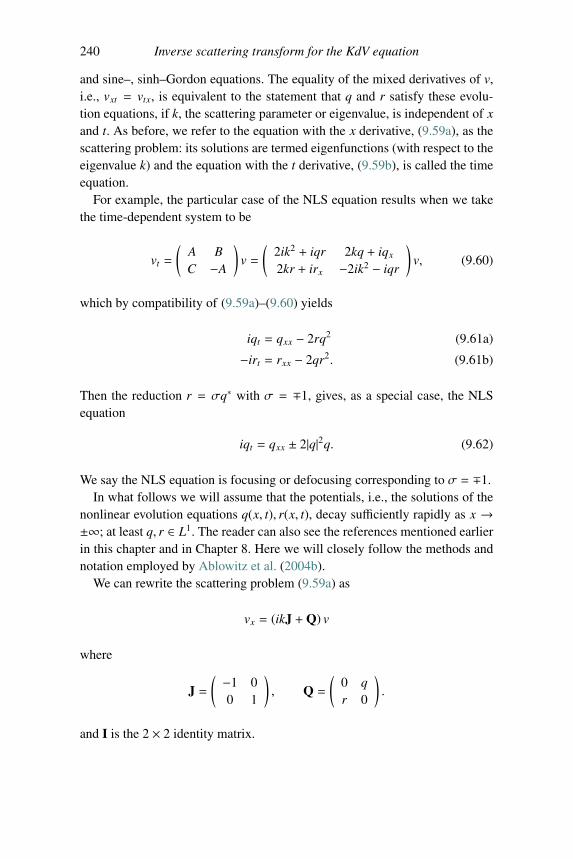
240 Inverse scattering transform for the KdV equation
and sine–, sinh–Gordon equations. The equality of the mixed derivatives of v,i.e., vxt = vtx, is equivalent to the statement that q and r satisfy these evolu-tion equations, if k, the scattering parameter or eigenvalue, is independent of xand t. As before, we refer to the equation with the x derivative, (9.59a), as thescattering problem: its solutions are termed eigenfunctions (with respect to theeigenvalue k) and the equation with the t derivative, (9.59b), is called the timeequation.
For example, the particular case of the NLS equation results when we takethe time-dependent system to be
vt =
(A BC −A
)v =
(2ik2 + iqr 2kq + iqx
2kr + irx −2ik2 − iqr
)v, (9.60)
which by compatibility of (9.59a)–(9.60) yields
iqt = qxx − 2rq2 (9.61a)
−irt = rxx − 2qr2. (9.61b)
Then the reduction r = σq∗ with σ = ∓1, gives, as a special case, the NLSequation
iqt = qxx ± 2|q|2q. (9.62)
We say the NLS equation is focusing or defocusing corresponding to σ = ∓1.In what follows we will assume that the potentials, i.e., the solutions of the
nonlinear evolution equations q(x, t), r(x, t), decay sufficiently rapidly as x →±∞; at least q, r ∈ L1. The reader can also see the references mentioned earlierin this chapter and in Chapter 8. Here we will closely follow the methods andnotation employed by Ablowitz et al. (2004b).
We can rewrite the scattering problem (9.59a) as
vx = (ikJ +Q) v
where
J =( −1 0
0 1
), Q =
(0 qr 0
).
and I is the 2 × 2 identity matrix.
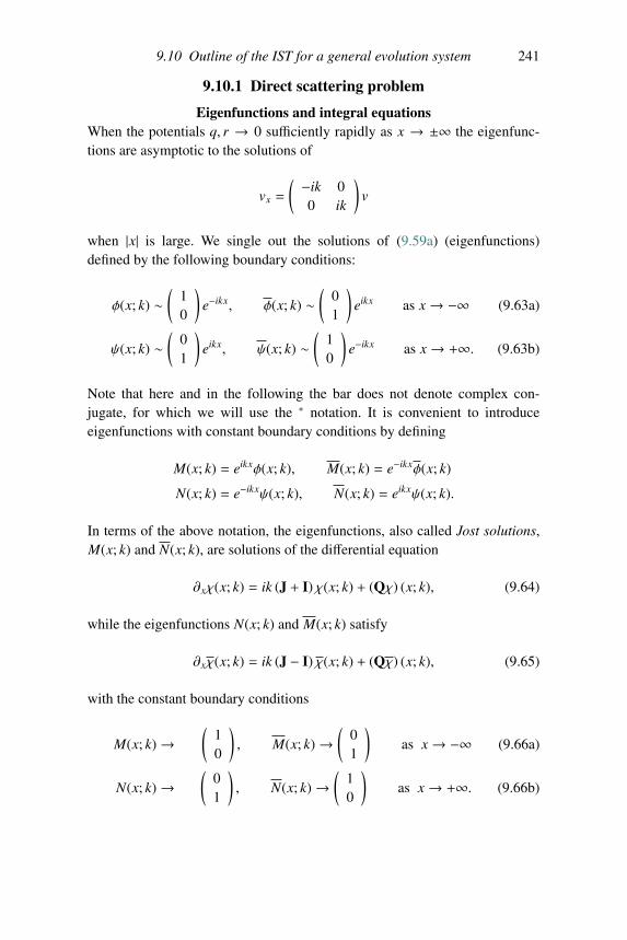
9.10 Outline of the IST for a general evolution system 241
9.10.1 Direct scattering problem
Eigenfunctions and integral equationsWhen the potentials q, r → 0 sufficiently rapidly as x → ±∞ the eigenfunc-tions are asymptotic to the solutions of
vx =
( −ik 00 ik
)v
when |x| is large. We single out the solutions of (9.59a) (eigenfunctions)defined by the following boundary conditions:
φ(x; k) ∼(
10
)e−ikx, φ(x; k) ∼
(01
)eikx as x→ −∞ (9.63a)
ψ(x; k) ∼(
01
)eikx, ψ(x; k) ∼
(10
)e−ikx as x→ +∞. (9.63b)
Note that here and in the following the bar does not denote complex con-jugate, for which we will use the ∗ notation. It is convenient to introduceeigenfunctions with constant boundary conditions by defining
M(x; k) = eikxφ(x; k), M(x; k) = e−ikxφ(x; k)
N(x; k) = e−ikxψ(x; k), N(x; k) = eikxψ(x; k).
In terms of the above notation, the eigenfunctions, also called Jost solutions,M(x; k) and N(x; k), are solutions of the differential equation
∂xχ(x; k) = ik (J + I) χ(x; k) + (Qχ) (x; k), (9.64)
while the eigenfunctions N(x; k) and M(x; k) satisfy
∂xχ(x; k) = ik (J − I) χ(x; k) + (Qχ) (x; k), (9.65)
with the constant boundary conditions
M(x; k)→(
10
), M(x; k)→
(01
)as x→ −∞ (9.66a)
N(x; k)→(
01
), N(x; k)→
(10
)as x→ +∞. (9.66b)
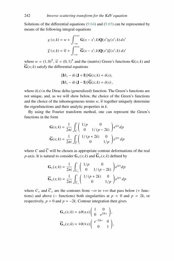
242 Inverse scattering transform for the KdV equation
Solutions of the differential equations (9.64) and (9.65) can be represented bymeans of the following integral equations
χ (x; k) = w +∫ +∞−∞
G(x − x′; k)Q(x′)χ(x′; k) dx′
χ (x; k) = w +∫ +∞−∞
G(x − x′; k)Q(x′)χ(x′; k) dx′
where w = (1, 0)T, w = (0, 1)T and the (matrix) Green’s functions G(x; k) andG(x; k) satisfy the differential equations
[I∂x − ik (J + I)] G(x; k) = δ(x),
[I∂x − ik (J − I)] G(x; k) = δ(x) ,
where δ(x) is the Dirac delta (generalized) function. The Green’s functions arenot unique, and, as we will show below, the choice of the Green’s functionsand the choice of the inhomogeneous terms w, w together uniquely determinethe eigenfunctions and their analytic properties in k.
By using the Fourier transform method, one can represent the Green’sfunctions in the form
G(x; k) =1
2πi
∫C
(1/p 0
0 1/ (p − 2k)
)eipxdp
G(x; k) =1
2πi
∫C
(1/ (p + 2k) 0
0 1/p
)eipx dp
where C and C will be chosen as appropriate contour deformations of the realp-axis. It is natural to consider G±(x; k) and G±(x; k) defined by
G±(x; k) =1
2πi
∫C±
(1/p 0
0 1/ (p − 2k)
)eipxdp
G±(x; k) =1
2πi
∫C±
(1/ (p + 2k) 0
0 1/p
)eipx dp
where C± and C± are the contours from −∞ to +∞ that pass below (+ func-tions) and above (− functions) both singularities at p = 0 and p = 2k, orrespectively, p = 0 and p = −2k. Contour integration then gives
G±(x; k) = ±θ(±x)
(1 00 e2ikx
),
G±(x; k) = ∓θ(∓x)
(e−2ikx 0
0 1
),
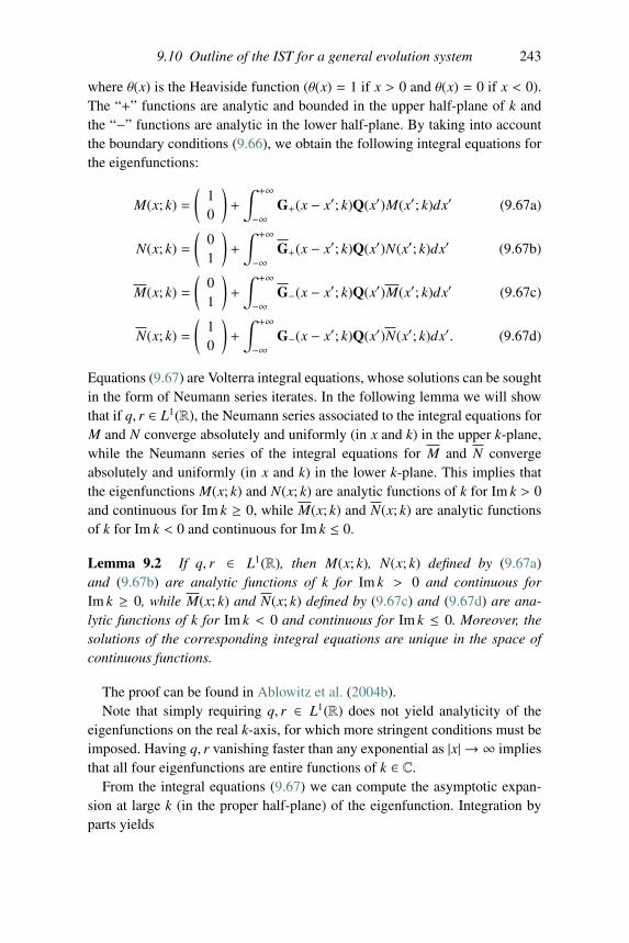
9.10 Outline of the IST for a general evolution system 243
where θ(x) is the Heaviside function (θ(x) = 1 if x > 0 and θ(x) = 0 if x < 0).The “+” functions are analytic and bounded in the upper half-plane of k andthe “−” functions are analytic in the lower half-plane. By taking into accountthe boundary conditions (9.66), we obtain the following integral equations forthe eigenfunctions:
M(x; k) =
(10
)+
∫ +∞−∞
G+(x − x′; k)Q(x′)M(x′; k)dx′ (9.67a)
N(x; k) =
(01
)+
∫ +∞−∞
G+(x − x′; k)Q(x′)N(x′; k)dx′ (9.67b)
M(x; k) =
(01
)+
∫ +∞−∞
G−(x − x′; k)Q(x′)M(x′; k)dx′ (9.67c)
N(x; k) =
(10
)+
∫ +∞−∞
G−(x − x′; k)Q(x′)N(x′; k)dx′. (9.67d)
Equations (9.67) are Volterra integral equations, whose solutions can be soughtin the form of Neumann series iterates. In the following lemma we will showthat if q, r ∈ L1(R), the Neumann series associated to the integral equations forM and N converge absolutely and uniformly (in x and k) in the upper k-plane,while the Neumann series of the integral equations for M and N convergeabsolutely and uniformly (in x and k) in the lower k-plane. This implies thatthe eigenfunctions M(x; k) and N(x; k) are analytic functions of k for Im k > 0and continuous for Im k ≥ 0, while M(x; k) and N(x; k) are analytic functionsof k for Im k < 0 and continuous for Im k ≤ 0.
Lemma 9.2 If q, r ∈ L1(R), then M(x; k), N(x; k) defined by (9.67a)and (9.67b) are analytic functions of k for Im k > 0 and continuous forIm k ≥ 0, while M(x; k) and N(x; k) defined by (9.67c) and (9.67d) are ana-lytic functions of k for Im k < 0 and continuous for Im k ≤ 0. Moreover, thesolutions of the corresponding integral equations are unique in the space ofcontinuous functions.
The proof can be found in Ablowitz et al. (2004b).Note that simply requiring q, r ∈ L1(R) does not yield analyticity of the
eigenfunctions on the real k-axis, for which more stringent conditions must beimposed. Having q, r vanishing faster than any exponential as |x| → ∞ impliesthat all four eigenfunctions are entire functions of k ∈ C.
From the integral equations (9.67) we can compute the asymptotic expan-sion at large k (in the proper half-plane) of the eigenfunction. Integration byparts yields
244 Inverse scattering transform for the KdV equation
M(x; k) =
(1 − 1
2ik
∫ x
−∞ q(x′)r(x′)dx′
− 12ik r(x)
)+ O(1/k2) (9.68a)
N(x; k) =
⎛⎜⎜⎜⎜⎝ 1 + 12ik
∫ +∞x
q(x′)r(x′)dx′
− 12ik r(x)
⎞⎟⎟⎟⎟⎠ + O(1/k2) (9.68b)
N(x; k) =
⎛⎜⎜⎜⎜⎝ 12ik q(x)
1 − 12ik
∫ +∞x
q(x′)r(x′)dx′
⎞⎟⎟⎟⎟⎠ + O(1/k2) (9.68c)
M(x; k) =
( 12ik q(x)
1 + 12ik
∫ x
−∞ q(x′)r(x′)dx′
)+ O(1/k2). (9.68d)
9.10.2 Scattering data
The two eigenfunctions with fixed boundary conditions as x → −∞ are lin-early independent, and the same holds for the two eigenfunctions with fixed
boundary conditions as x → +∞. Indeed, let u(x, k) =(u(1)(x, k), u(2)(x, k)
)Tand v(x, k) =
(v(1)(x, k), v(2)(x, k)
)Tbe any two solutions of (9.59a) and let us
define the Wronskian of u and v, W(u, v), as
W(u, v) = u(1)v(2) − u(2)v(1).
Using (9.59a) it can be verified that
ddx
W(u, v) = 0
where W(u, v) is a constant. Therefore, from the prescribed asymptotic behav-ior for the eigenfunctions, it follows that
W(φ, φ)= lim
x→−∞W(φ(x; k), φ(x; k)
)= 1
W(ψ, ψ)= lim
x→+∞W(ψ(x; k), ψ(x; k)
)= −1,
which shows that the solutions φ and φ are linearly independent, as are ψ andψ. As a consequence, we can express φ(x; k) and φ(x; k) as linear combina-tions of ψ(x; k) and ψ(x; k), or vice versa, with the coefficients of these linearcombinations depending on k only. Hence, the relations
φ(x; k) = b(k)ψ(x; k) + a(k)ψ(x; k) (9.69a)
φ(x; k) = a(k)ψ(x; k) + b(k)ψ(x; k) (9.69b)
hold for any k ∈ C such that the four eigenfunctions exist. In particular, (9.69)hold for Im k = 0 and define the scattering coefficients a(k), a(k), b(k), b(k) for
9.10 Outline of the IST for a general evolution system 245
k ∈ R. Comparing the asymptotics of W(φ, φ) as x → ±∞ with (9.69) showsthat the scattering data satisfy the following equation:
a(k)a(k) − b(k)b(k) = 1 ∀k ∈ R.The scattering coefficients can, in turn, be represented as Wronskians of theeigenfunctions. Indeed, from (9.69) it follows that
a(k) = W(φ, ψ), a(k) = W(ψ, φ) (9.70a)
b(k) = W(ψ, φ), b(k) = W(φ, ψ). (9.70b)
Therefore, if q, r ∈ L1(R), Lemma 9.2 and equations (9.70) imply that a(k)admit analytic continuation in the upper half k-plane, while a(k) can be analyt-ically continued in the lower half k-plane. In general, b(k) and b(k) cannot beextended off the real k-axis. It is also possible to obtain integral representationsfor the scattering coefficients in terms of the eigenfunctions, but we will not doso here.
Equation (9.69) can be written as
μ(x, k) = N(x; k) + ρ(k)e2ikxN(x; k) (9.71a)
μ(x, k) = N(x; k) + ρ(k)e−2ikxN(x; k), (9.71b)
where we introduced
μ(x, k) = M(x; k)/a(k), μ(x, k) = M(x; k)/a(k) (9.72)
and the reflection coefficients
ρ(k) = b(k)/a(k), ρ(k) = b(k)/a(k). (9.73)
Note that from the representation of the scattering data as Wronskians of theeigenfunctions and from the asymptotic expansions (9.68), it follows that
a(k) = 1 + O(1/k), a(k) = 1 + O(1/k)
in the proper half-plane, while b(k), b(k) are O(1/k) as |k| → ∞ on the realaxis. We further assume that a(k), a(k) are continuous for real k. Since a(k) isanalytic for Im k > 0, continuous for Im k = 0 and a(k)→ 1 for |k| → ∞, therecannot be a cluster point of zeros for Im k ≥ 0. Hence the number of zeros isfinite. Similarly for a(k).
Proper eigenvalues and norming constantsA proper (or discrete) eigenvalue of the scattering problem (9.59a) is a (com-plex) value of k corresponding to a bounded solution v(x, k) such that v(x, k)→0 as x → ±∞; usually one requires v ∈ L2(R) with respect to x. We also callsuch solutions bound states. When q = r∗ in (9.59a), the scattering problem is
246 Inverse scattering transform for the KdV equation
self-adjoint and there are no eigenvalues/bound states. So the only possibilityfor eigenvalues is when q = −r∗. We will see that these eigenvalues correspondto solitons that decay rapidly at infinity; sometimes called “bright” solitons.The so-called “dark” solitons, which tend to constant states at infinity, are con-tained in an extended theory (cf. Zakharov and Shabat, 1973; Prinari et al.,2006).
Suppose that k j = ξ j + iη j, with η j > 0, is such that a(k j) = 0. Thenfrom (9.70a) it follows that W(φ(x; k j), ψ(x; k j)) = 0 and therefore φ j(x) :=φ(x; k j) and ψ j(x) = ψ(x; k j) are linearly dependent; that is, there exists acomplex constant c j such that
φ j(x) = c jψ j(x).
Hence, by (9.63a) and (9.63b) it follows that
φ j(x) ∼(
10
)eη j x−iξ j x as x→ −∞
φ j(x) = c jψ j(x) ∼(
01
)e−η j x+iξ j x as x→ +∞.
Since we have strong decay for large |x|, it follows that k j is a propereigenvalue. On the other hand, if a(k) � 0 for Im k > 0, then solutions ofthe scattering problem blow up in one or both directions. We conclude thatthe proper eigenvalues in the region Im k > 0 are precisely the zeros of thescattering coefficient a(k). Similarly, the eigenvalues in the region Im k < 0are given by the zeros of a(k), and these zeros k j = ξ j + iη j are such that
φ(x; k j) = c jψ(x; k j) for some complex constant c j. The coefficients{c j
}Jj=1
and{c j
}Jj=1
are often called norming constants. In terms of the eigenfunctions,
the norming constants are defined by
Mj(x) = c j e2ik j xN j(x) , M j(x) = c j e−2ik j xN j(x) , (9.74)
where Mj(x) = M(x; k j), M j(x) = M(x; k j) and similarly for Nj(x) and N j(x).As we will see in the following, discrete eigenvalues and associated normingconstants are part of the scattering data (i.e., the data necessary to uniquelysolve the inverse problem and reconstruct q(x, t) and r(x, t)).
Note that if the potentials q, r are rapidly decaying, such that (9.69) can beextended off the real axis, then
c j = b(k j) for j = 1, . . . , J
c j = b(k j) for j = 1, . . . , J.
9.10 Outline of the IST for a general evolution system 247
Symmetry reductionsThe NLS equation is a special case of the system (9.61) under the symme-try reduction r = ±q∗. This symmetry in the potentials induces a symmetrybetween the eigenfunctions analytic in the upper k-plane and the ones ana-lytic in the lower k-plane. In turn, this symmetry of the eigenfunctions inducessymmetries in the scattering data.
Indeed, if v(x, k) =(v(1)(x, k), v(2)(x, k)
)Tsatisfies (9.59a) and r = ∓q∗, then
v(x, k) =(v(2)(x, k∗),∓v(1)(x, k∗)
)†(where † denotes conjugate transpose) also
satisfies the same (9.59a). Taking into account the boundary conditions (9.63),we get
ψ(x; k) =
(ψ(2)(x; k∗)∓ψ(1)(x; k∗)
)∗, φ(x; k) =
( ∓φ(2)(x; k∗)φ(1)(x; k∗)
)∗,
N(x; k) =
(N(2)(x; k∗)∓N(1)(x; k∗)
)∗, M(x; k) =
( ∓M(2)(x; k∗)M(1)(x; k∗)
)∗.
Then, from the Wronskian representations for the scattering data (9.70) therefollows
a(k) = a∗(k∗) , b(k) = ∓b∗(k∗) ,
which implies that k j is a zero of a(k) in the upper half k-plane if and only if k∗jis a zero of a(k) in the lower k-plane and vice versa. This means that the zerosof a(k) and a(k) come in pairs and the number of zeros of each is the same, i.e.,J = J. Hence when there are eigenvalues associated with the potential q, withq = −r∗, we have that
k j = k∗j , c j = ∓c∗j j = 1, . . . , J.
On the other hand, if we have the symmetry r = ∓q, with q real, then
v(x, k) =(v(2)(x,−k),∓v(1)(x,−k)
)Talso satisfies the same equation (9.59a).
Taking into account the boundary conditions (9.63), we get
ψ(x; k) =
(ψ(2)(x;−k)∓ψ(1)(x;−k)
), φ(x; k) =
( ∓φ(2)(x;−k)φ(1)(x;−k)
),
N(x; k) =
(N(2)(x;−k)∓N(1)(x;−k)
), M(x; k) =
( ∓M(2)(x;−k)M(1)(x;−k)
).
Then, from the Wronskian representations for the scattering data (9.70), therefollows
a(k) = a(−k) , b(k) = ∓b(−k) , (9.75)
which implies that k j is a zero of a(k) in the upper half k-plane if and only if−k j is a zero of a(k) in the lower k-plane, and vice versa. As a consequence,
248 Inverse scattering transform for the KdV equation
when r = −q, with q real, the zeros of a(k) and a(k) are paired, their number isthe same: J = J and
k j = −k j , c j = −c j j = 1, . . . , J. (9.76)
Thus if r = −q, with q real, both of the above symmetry conditions must holdand when k j is an eigenvalue so is −k∗j ; i.e., either the eigenvalues come inpairs, {k j,−k∗j}, or they lie on the imaginary axis.
9.10.3 Inverse scattering problem
The inverse problem consists of constructing a map from the scattering data,that is:
(i) the reflection coefficients ρ(k) and ρ(k) for k ∈ R, defined by (9.73);
(ii) the discrete eigenvalues{k j
}Jj=1
(zeros of the scattering coefficient a(k) in
the upper half plane of k) and{k j
}Jj=1
(zeros of the scattering coefficient
a(k) in the lower half plane of k);
(iii) the norming constants{c j
}Jj=1
and{c j
}Jj=1
, cf. (9.74); back to the potentials
q and r.First, we use these data to reconstruct the eigenfunctions (for instance, N(x; k)and N(x; k)), and then we recover the potentials from the large k asymptoticsof the eigenfunctions, cf. equations (9.68). Note that the inverse problem issolved at fixed t, and therefore the explicit time dependence is omitted. In fact,in the inverse problem both x and t are treated as parameters.
Riemann–Hilbert approachIn the previous section, we showed that the eigenfunctions N(x; k) and N(x; k)exist and are analytic in the regions Im k > 0 and Im k < 0, respectively, ifq, r ∈ L1(R). Similarly, under the same conditions on the potentials, the func-tions μ(x, k) and μ(x, k) introduced in (9.72) are meromorphic in the regionsIm k > 0 and Im k < 0, respectively, with poles at the zeros of a(k) anda(k). Therefore, in the inverse problem we assume these analyticity propertiesfor the unknown eigenfunctions (N(x; k) and N(x; k)) or modified eigenfunc-tions (μ(x, k) and μ(x, k)). With these assumptions, (9.71) can be consideredas the “jump” conditions of a Riemann–Hilbert problem. To recover the sec-tionally meromorphic functions from the scattering data, we will convert theRiemann–Hilbert problem into a system of linear integral equations.
Suppose that a(k) and a(k) have a finite number of simple zeros in the regions
Im k > 0 and Im k < 0, respectively, which we denote as{k j, Im k j > 0
}Jj=1
and
9.10 Outline of the IST for a general evolution system 249{k j, Im k j < 0
}Jj=1
. We will also assume that a(ξ) � 0 and a(ξ) � 0 for ξ ∈ R(i.e., a and a have no zeros on the real axis) and a(k) is continuous for Im k ≥ 0.
Let f (ζ), ζ ∈ R, be an integrable function and consider the projectionoperators
P±[ f ](k) =1
2πi
∫ +∞−∞
f (ζ)ζ − (k ± i0)
dζ.
If f+ (resp. f−) is analytic in the upper (resp. lower) k-plane and f±(k) → 0 as|k| → ∞ for Im k ≷ 0, then
P±[f±]= ± f±, P±
[f∓]= 0
[P± are referred to as projection operators into the upper/lower half k-planes].Let us now apply the projector P− to both sides of (9.71a) and P+ to bothsides of (9.71b). Note that μ(x, k) = M(x; k)/a(k) in (9.71a) does not decayfor large k; rather it tends to (1, 0)T. In addition it has poles at the zeros ofa(k). We subtract these contributions from both sides of (9.71a) and then takethe projector; similar statements apply to μ(x, k) in (9.71b). So, taking intoaccount the analyticity properties of N, N, μ, μ and the asymptotics (9.68) andusing (9.74), we obtain
N(x; k) =
⎛⎜⎜⎜⎜⎝ 10
⎞⎟⎟⎟⎟⎠ + J∑j=1
C je2ik j x
k − k jN j(x) +
12πi
∫ +∞−∞
ρ(ζ)e2iζx
ζ − (k − i0)N(x; ζ) dζ (9.77a)
N(x; k) =
⎛⎜⎜⎜⎜⎝ 01
⎞⎟⎟⎟⎟⎠ + J∑j=1
C je−2ik j x
k − k j
N j(x) − 12πi
∫ +∞−∞
ρ(ζ)e−2iζx
ζ − (k + i0)N(x; ζ) dζ, (9.77b)
where Nj(x) = N(x; k j), N j(x) = N(x; k j) and we introduced
C j =c j
a′(k j)for j = 1, . . . , J
C j =c j
a′(k j)for j = 1, . . . , J
with ′ denoting the derivative of a(k) and a(k) with respect to k. We see thatthe equations defining the inverse problem for N(x; k) and N(x; k) depend on
the extra terms{Nj(x)
}Jj=1
and{N j(x)
}Jj=1
. In order to close the system, we
evaluate (9.77a) at k = k j for j = 1, . . . , J and (9.77b) at k = k j for j = 1, . . . , J,thus obtaining
250 Inverse scattering transform for the KdV equation
N�(x) =
⎛⎜⎜⎜⎜⎝ 10
⎞⎟⎟⎟⎟⎠ + J∑j=1
C je2ik j x
k� − k j
N j(x) +1
2πi
∫ +∞−∞
ρ(ζ)e2iζx
ζ − k�N(x; ζ) dζ (9.78a)
Nj(x) =
⎛⎜⎜⎜⎜⎝ 01
⎞⎟⎟⎟⎟⎠ + J∑m=1
Cme−2ikm x
k j − km
N j(x) − 12πi
∫ +∞−∞
ρ(ζ)e−2iζx
ζ − k jN(x; ζ) dζ . (9.78b)
Equations (9.77) and (9.78) together constitute a linear algebraic – integralsystem of equations that, in principle, solve the inverse problem for theeigenfunctions N(x; k) and N(x; k).
By comparing the asymptotic expansions at large k of the right-hand sidesof (9.77) with the expansions (9.68), we obtain
r(x) = −2iJ∑
j=1
e2ik j xC jN(2)j (x) +
1π
∫ +∞−∞
ρ(ζ)e2iζxN(2)(x; ζ) dζ (9.79a)
q(x) = 2iJ∑
j=1
e−2ik j xC jN(1)j (x) +
1π
∫ +∞−∞
ρ(ζ)e−2iζxN(1)
(x; ζ)dζ (9.79b)
which reconstruct the potentials in terms of the scattering data and thus com-plete the formulation of the inverse problem (as before, the superscript (�)
denotes the �-component of the corresponding vector).We mention that the issue of establishing existence and uniqueness of
solutions for the equations of the inverse problem is usually carried out by con-verting the inverse problem into a set of Gelfand–Levitan–Marchenko integralequations – which is given next.
Gel’fand–Levitan–Marchenko integral equationsAs an alternative inverse procedure we provide a reconstruction for thepotentials by developing the Gel’fand–Levitan–Marchenko (GLM) integralequations, instead of using the projection operators (cf. Zakharov and Shabat,1972; Ablowitz and Segur, 1981). To do this we represent the eigenfunctionsin terms of triangular kernels
N(x; k) =
(01
)+
∫ +∞x
K(x, s)e−ik(x−s) ds, s > x, Im k > 0 (9.80)
N(x; k) =
(10
)+
∫ +∞x
K(x, s)eik(x−s) ds, s > x, Im k < 0. (9.81)
9.10 Outline of the IST for a general evolution system 251
Applying the operator 12π
∫ +∞−∞ dk e−ik(x−y) for y > x to (9.77a), we find
K(x, y) +
(01
)F(x + y) +
∫ +∞
xK(x, s)F(s + y) ds = 0 (9.82)
where
F(x) =1
2π
∫ +∞−∞
ρ(ξ)eiξx dξ − iJ∑
j=1
C jeik j x.
Analogously, operating on (9.77b) with 12π
∫ +∞−∞ dk eik(x−y) for y > x gives
K(x, y) +
(10
)F(x + y) +
∫ +∞x
K(x, s)F(s + y) ds = 0 (9.83)
where
F(x) =1
2π
∫ +∞−∞
ρ(ξ)e−iξx dξ + iJ∑
j=1
C je−ik j x.
Equations (9.82) and (9.83) constitute the Gel’fand–Levitan–Marchenko equa-tions.
Inserting the representations (9.80)–(9.81) for the eigenfunctions into (9.79)we obtain the reconstruction of the potentials in terms of the kernels of theGLM equations, i.e.,
q(x) = −2K(1)(x, x), r(x) = −2K(2)
(x, x) (9.84)
where, as usual, K( j) and K( j)
for j = 1, 2 denote the jth component of thevectors K and K respectively.
If the symmetry r = ∓q∗ holds, then, taking into account (9.75)–(9.76), onecan verify that
F(x) = ∓F∗(x)
and consequently
K(x, y) =
(K(2)(x, y)∓K(1)(x, y)
)∗.
In this case (9.82)–(9.83) solving the inverse problem reduce to
K(1)(x, y) = ±F∗(x + y) ∓∫ +∞
xds∫ +∞
xds′K(1)(x, s′)F(s + s′)F∗(y + s)
and the potentials are reconstructed by means of the first of (9.84). We alsonote that when r = ∓q with q real, then F(x) and K(1)(x, y) are real.
252 Inverse scattering transform for the KdV equation
9.10.4 Time evolution
We will now show how to determine the time dependence of the scattering data.Then, by the inverse transform we establish the solution q(x, t) and r(x, t).
The operator equation (9.59b) determines the evolution of the eigenfunc-tions, which can be written as
∂tv =
(A BC −A
)v (9.85)
where B,C → 0 as x → ±∞ (since q, r ∈ L1(R)). Then the time-dependenteigenfunctions must asymptotically satisfy the differential equation
∂tv =
(A0 00 −A0
)v as x→ ±∞ (9.86)
with
A0 = lim|x|→∞
A(x, k).
The system (9.86) has solutions that are linear combinations of
v+ =
(eA0t
0
), v− =
(0
e−A0t
).
However, such solutions are not compatible with the fixed boundary conditionsof the eigenfunctions, i.e., equations (9.63a)–(9.63b). Therefore, we definetime-dependent functions
Φ(x, t; k) = eA0tφ (x, t; k) , Φ(x, t; k) = e−A0tφ(x, t; k)
Ψ(x, t; k) = e−A0tψ (x, t; k) , Ψ(x, t; k) = eA0tψ(x, t; k)
to be solutions of the differential equation (9.85). Then the evolution for φ andφ becomes
∂tφ =
(A − A0 B
C −A − A0
)φ, ∂tφ =
(A + A0 B
C −A + A0
)φ, (9.87)
so that, taking into account (9.69) and evaluating (9.87) as x→ +∞, we obtain
∂ta = 0, ∂ta = 0
∂tb = −2A0b, ∂tb = 2A0b
or, explicitly,
a(k, t) = a(k, 0), a(k, t) = a(k, 0) (9.88a)
b(k, t) = b(k, 0)e−2A0(k)t, b(k, t) = b(k, 0)e2A0(k)t. (9.88b)
9.10 Outline of the IST for a general evolution system 253
From (9.88a) it follows that the discrete eigenvalues (i.e., the zeros of a anda) are constant as the solution evolves. Not only the number of eigenvalues,but also their locations are fixed. Thus, the eigenvalues are time-independentdiscrete states of the evolution. In fact, this time invariance is the underlyingmechanism of the elastic soliton interaction for the integrable soliton equa-tions. On the other hand, the evolution of the reflection coefficients (9.73) isgiven by
ρ(k, t) = ρ(k, 0)e−2A0(k)t, ρ(k, t) = ρ(k, 0)e2A0(k)t
and this also gives the evolution of the norming constants:
C j(t) = C j(0)e−2A0(k j)t, C j(t) = C j(0)e2A0(k j)t. (9.89)
The expressions for the evolution of the scattering data allow one to solve theinitial value problem for all of the solutions in the class associated with thescattering problem (9.59a). Namely we can solve (see the previous chapter fordetails) all the equations in the class given by the general evolution operator(
r−q
)t
+ 2A0(L)
(rq
)= 0, (9.90)
where A0(k) = lim|x|→∞ A(x, t, k) (here A0(k) may be the ratio of two entirefunctions), and L is the integro-differential operator given by
L =12i
(∂x − 2r(I−q) 2r(I−r)−2q(I−q) −∂x + 2q(I−r)
),
where ∂x ≡ ∂/∂x and
(I− f )(x) ≡∫ x
−∞f (y) dy. (9.91)
Note that L operates on (r, q), and I− operates both on the functions immedi-ately to its right and also on the functions to which L is applied.
Special cases are listed below:
• When A0 = 2ik2, r = ∓q∗ we obtain the solution of the NLS equation
iqt = qxx ± 2|q|2q
i.e., (9.62).• If A0 = −4ik3 when r = ∓q, q real we find the solution of the modified KdV
(mKdV) equation,
qt ± 6q2qx + qxxx = 0. (9.92)
254 Inverse scattering transform for the KdV equation
• If on the other hand r = ∓q∗ the solution of the complex mKdV equationresults:
qt ± 6|q|2qx + qxxx = 0.
• Finally, if A0 =i
4k and(i) q = −r = − 1
2 ux, we obtain the solution of the sine – Gordon equation
uxt = sin u; (9.93)
(ii) or, if q = r = 12 ux, then we can find the solution of the sinh–Gordon
equation
uxt = sinh u.
In summary the solution procedure is as follows:(i) The scattering data are calculated from the initial data q(x) = q(x, 0)
and r(x) = r(x, 0) according to the direct scattering method describedin Section 9.10.1.
(ii) The scattering data at a later time t > 0 are determined from (9.88)–(9.89).(iii) The solutions q(x, t) and r(x, t) are recovered from the scattering
data using inverse scattering using the reconstruction formulas viathe Riemann–Hilbert formulation (9.77)–(9.79) or Gel-fand–Levitan–Marchenko equations (9.82)–(9.83).
If we further require symmetry, r = ±q∗, as discussed in the above section onsymmetry reductions, we obtain the solution of the reduced evolution equation.
9.10.5 Soliton solutions
In the case where the scattering data comprise proper eigenvalues but ρ(k) =ρ(k) ≡ 0 for all k ∈ R (corresponding to the so-called reflectionless solutions),the algebraic-integral system (9.77) and (9.78) reduces to a linear algebraicsystem, namely
Nl(x) =
(10
)+
J∑j=1
C je2ik j xN j(x)
kl − k j
N j(x) =
(01
)+
J∑m=1
Cme−2ikm xNm(x)
k j − km
,
that can be solved in closed form. The one-soliton solution, in particular, isobtained for J = J = 1 (i.e., one single discrete eigenvalue k1 = ξ + iη and
9.10 Outline of the IST for a general evolution system 255
corresponding norming constant C1). In the relevant physical case, when thesymmetry r = −q∗ holds, using (9.75) and (9.76) in the above system, we get
N(1)1 (x) = − C1
k1 − k∗1e−2ik∗1 x
⎡⎢⎢⎢⎢⎢⎢⎢⎢⎣1 − |C1|2 e2i(k1−k∗1)x(k1 − k∗1
)2⎤⎥⎥⎥⎥⎥⎥⎥⎥⎦−1
,
N(2)1 (x) =
⎡⎢⎢⎢⎢⎢⎢⎢⎢⎣1 − |C1|2 e2i(k1−k∗1)x(k1 − k∗1
)2⎤⎥⎥⎥⎥⎥⎥⎥⎥⎦−1
,
where, as before, N1(x) =(N(1)
1 (x),N(2)1 (x)
)T. Then, if we set
k1 = ξ + iη, e2δ =|C1|2η
,
it follows from (9.79) that
q(x) = −2iηC∗1|C1|e
−2iξx sech (2ηx − 2δ) .
Taking into account the time dependence of C1 as given by (9.89), we find
q(x) = 2ηe−2iξx+2i Im A0(k1)t−iψ0 sech[2 (η(x − x0) + Re A0(k1)t)
],
where C1(0) = 2ηe2ηx0+i(ψ0+π/2).Thus when we take
(a) A0(k1) = 2ik21 = −4ξη + 2i(ξ2 − η2) where k1 = ξ + iη, r = −q∗ we get the
well-known bright soliton solution of the NLS equation
q(x, t) = 2ηe−2iξx+4i(ξ2−η2)t−iψ0 sech[2η (x − 4ξt − x0)
].
(b) A0(k1) = −4ik31 = −4η3 where k1 = iη, r = −q, real; recall that due to
symmetry all eigenvalues must come in pairs{k j,−k∗j
}hence with only
one eigenvalue Re k1 = ξ = 0. Then we get the bright soliton solution ofthe mKdV equation (9.92):
q(x, t) = 2η sech[2η(x − 4η2t − x0
)].
(c) A0(k1) = i4k =
14η where k1 = iη, r = −q = ux
2 , real; again due to symmetryRe k1 = ξ = 0. Then we get the soliton-kink solution of the sine–Gordonequation (9.93):
q(x, t) = −ux
2= −2η sech
[2η
(x +
14η
t − x0
)],
or in terms of u
u(x, t) = 4 tan−1 exp
[2η
(x +
14η
t − x0
)].
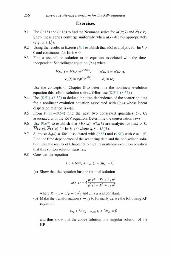
256 Inverse scattering transform for the KdV equation
Exercises
9.1 Use (9.15) and (9.16) to find the Neumann series for M(x; k) and N(x; k).Show these series converge uniformly when u(x) decays appropriately(e.g., u ∈ L1
2).9.2 Using the results in Exercise 9.1 establish that a(k) is analytic for Im k >
0 and continuous for Im k = 0.9.3 Find a one-soliton solution to an equation associated with the time-
independent Schrodinger equation (9.4) when
b(k, t) = b(k, 0)e−32ik5t, a(k, t) = a(k, 0),
c j(t) = c j(0)e32k5j t, k j = iκ j.
Use the concepts of Chapter 8 to determine the nonlinear evolutionequation this soliton solution solves. (Hint: use (8.51)–(8.52).)
9.4 Use (8.51)–(8.52) to deduce the time-dependence of the scattering datafor a nonlinear evolution equation associated with (9.4) whose lineardispersion relation is ω(k).
9.5 From (9.53)–(9.54) find the next two conserved quantities C7, C9
associated with the KdV equation. Determine the conservation laws.9.6 Use (9.67) to establish that M(x; k), N(x; k) are analytic for Im k > 0,
M(x; k), N(x; k) for Im k < 0 where q, r ∈ L1(R).9.7 Suppose A0(k) = 8ik4, associated with (9.85) and (9.90) with r = −q∗.
Find the time dependence of the scattering data and the one-soliton solu-tion. Use the results of Chapter 8 to find the nonlinear evolution equationthat this soliton solution satisfies.
9.8 Consider the equation
(ut + 6uux + uxxx)x − 3uyy = 0.
(a) Show that the equation has the rational solution
u(x, t) = 4p2y2 − X2 + 1/p2
p2y2 + X2 + 1/p2
where X = x + 1/p − 3p2t and p is a real constant.(b) Make the transformation y→ iy to formally derive the following KP
equation
(ut + 6uux + uxxx)x + 3uyy = 0
and thus show that the above solution is a singular solution of theKP.
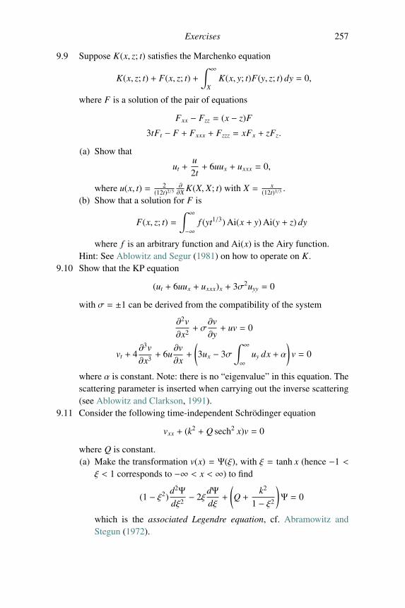
Exercises 257
9.9 Suppose K(x, z; t) satisfies the Marchenko equation
K(x, z; t) + F(x, z; t) +∫ ∞
XK(x, y; t)F(y, z; t) dy = 0,
where F is a solution of the pair of equations
Fxx − Fzz = (x − z)F
3tFt − F + Fxxx + Fzzz = xFx + zFz.
(a) Show that
ut +u2t+ 6uux + uxxx = 0,
where u(x, t) = 2(12t)2/3
∂∂X K(X, X; t) with X = x
(12t)1/3 .(b) Show that a solution for F is
F(x, z; t) =∫ ∞
−∞f (yt1/3) Ai(x + y) Ai(y + z) dy
where f is an arbitrary function and Ai(x) is the Airy function.Hint: See Ablowitz and Segur (1981) on how to operate on K.
9.10 Show that the KP equation
(ut + 6uux + uxxx)x + 3σ2uyy = 0
with σ = ±1 can be derived from the compatibility of the system
∂2v∂x2+ σ
∂v∂y+ uv = 0
vt + 4∂3v∂x3+ 6u
∂v∂x+
(3ux − 3σ
∫ ∞
∞uy dx + α
)v = 0
where α is constant. Note: there is no “eigenvalue” in this equation. Thescattering parameter is inserted when carrying out the inverse scattering(see Ablowitz and Clarkson, 1991).
9.11 Consider the following time-independent Schrodinger equation
vxx + (k2 + Q sech2 x)v = 0
where Q is constant.(a) Make the transformation v(x) = Ψ(ξ), with ξ = tanh x (hence −1 <
ξ < 1 corresponds to −∞ < x < ∞) to find
(1 − ξ2)d2Ψ
dξ2− 2ξ
dΨdξ+
(Q +
k2
1 − ξ2
)Ψ = 0
which is the associated Legendre equation, cf. Abramowitz andStegun (1972).
258 Inverse scattering transform for the KdV equation
(b) Show that there are eigenvalues k = iκ when
κ =
⎡⎢⎢⎢⎢⎢⎣(Q + 14
)1/2− m − 1
2
⎤⎥⎥⎥⎥⎥⎦ > 0,
where m = 0, 1, 2, . . . and therefore a necessary condition foreigenvalues is Q + 1
4 >14 .
(c) Show that when Q = N(N + 1),N = 1, 2, 3, . . ., the reflection coef-ficient vanishes, the discrete eigenvalues are given by κn = n, n =1, 2, 3, . . . ,N and the discrete eigenfunctions are proportional to theassociated Legendre function Pn
N(tanh x).9.12 Show that the solution to the Gel’fand–Levitan–Marchenko (GLM)
equation (9.42)–(9.43) with pure continuous spectra is unique. Hint: onemethod is to show the homogeneous equation has only the zero solution,hence by the Fredholm alternative, the solution to the GLM equation isunique. Then in the homogeneous equation let K(x, y) = 0, y < x andtake the Fourier transform.
PART III
APPLICATIONS OF NONLINEAR WAVES INOPTICS

10Communications
Nonlinear optics is the branch of optics that describes the behavior of lightin nonlinear media; such as, media in which the induced dielectric polariza-tion responds nonlinearly to the electric field of the light. This nonlinearityis typically observed at very high light intensities such as those provided bypulsed lasers. In this chapter, we focus on the application of high bit-ratecommunications. We will see that the nonlinear Schrodinger (NLS) equationand the dispersion-managed nonlinear Schrodinger (DMNLS) equation play acentral role.
10.1 Communications
In 1973 Hasegawa and Tappert (Hasegawa and Tappert, 1973a; Hasegawaand Kodama, 1995) showed that the nonlinear Schrodinger equation derivedin Chapter 7 [see (7.26), and the subsequent discussion] described the prop-agation of quasi-monochromatic pulses in optical fibers. Motivated by thefact that the NLS equation supports special stable, localized, soliton solu-tions, Mollenauer et al. (1980) demonstrated experimentally that solitonscan propagate in a real fiber. However, it was soon apparent that due tounavoidable damping in optical fibers, solitons lose most of their energyover relatively short distances. In the mid-1980s all-optical amplifiers (callederbium doped fiber amplifiers: EDFAs) were developed. However with suchamplifiers there is always some additional small amount of noise. Gordon andHaus (1986) (see also Elgin, 1985) showed that solitons suffered seriously fromthese noise effects. The frequency and temporal position of the soliton wassignificantly shifted over long distances, thereby limiting the available trans-mission distance and speed of soliton-based systems. Subsequently researchersbegan to seriously consider so-called wavelength division multiplexed (WDM)
261
262 Communications
communication systems in which many optical pulses are transmitted simul-taneously. The inevitable pulse interactions caused other serious problems,called four-wave mixing instabilities and collision-induced time shifts. In orderto alleviate these penalties, researchers began to study dispersion-managed(DM) transmission systems. A DM transmission line consists of fibers withdifferent types of dispersion fused together. The success of DM technologyhas already led to its use in commercial systems. In this chapter we discusssome of the important issues in the context of nonlinear waves and asymp-totic analysis. There are a number of texts that cover this topic, which theinterested reader can consult. These include Agrawal (2002, 2001), Hasegawaand Kodama (1995), Hasegawa and Matsumoto (2002), and Molleneauer andGordon (2006).
10.1.1 The normalized NLS equation
In Chapter 7 the NLS equation was derived for weakly nonlinear, quasi-monochromatic electromagnetic waves. It was also discussed how the NLSequation should be modified to apply to optical fibers. Using the assumptionfor electromagnetic fields in the x-direction
Ex = ε(A(Z,T )ei(kz−ωt) + cc) + O(ε2),
where Z = εz, T = εt, the NLS equation in optical fibers was found, in Chapter7 [see (7.27) and the equations following], to satisfy
i∂A∂z+
(−k′′(ω)
2
)∂2A∂T 2+ ν|A|2A = 0, (10.1)
with the nonlinear coefficient ν = νeff =n2ω
4cAeffwhere the retarded coordinate
frame is given by T = εt − Zvg= εt − k′Z, z = εZ with k =
ω
cn0, and the
nonlinear index of refraction is given by n = n0 + n2|Ex|2 = n0 + 4n2|A|2;vg = 1/k′(ω) is the group velocity and Aeff is the effective area of the fiber. Itis standard to introduce the following non-dimensional coordinates: z = z′z∗,T = t′t∗, and A =
√P∗u, where a subscript ∗ denotes a characteristic scale.
Usually, z∗ is taken as being proportional to the nonlinear length, the lengthover which a nonlinear phase change of one radian occurs, t∗ is taken as beingproportional to the pulse full width at half-maximum (FWHM), and P∗ is takenas the peak pulse power. With the use of this non-dimensionalization, (10.1)becomes
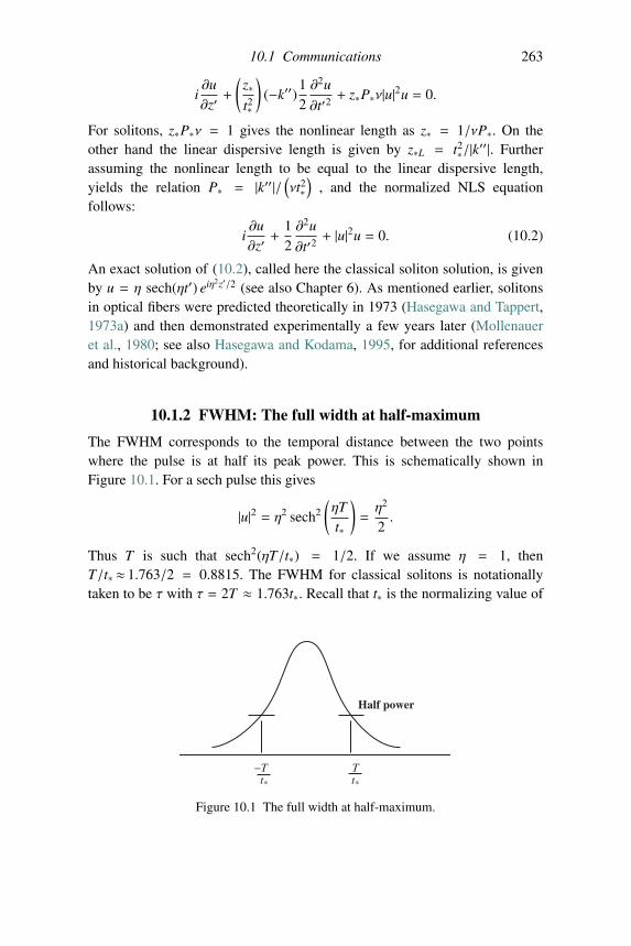
10.1 Communications 263
i∂u∂z′+
(z∗t2∗
)(−k′′)
12∂2u
∂t′2+ z∗P∗ν|u|2u = 0.
For solitons, z∗P∗ν = 1 gives the nonlinear length as z∗ = 1/νP∗. On theother hand the linear dispersive length is given by z∗L = t2∗/|k′′|. Furtherassuming the nonlinear length to be equal to the linear dispersive length,yields the relation P∗ = |k′′|/
(νt2∗)
, and the normalized NLS equationfollows:
i∂u∂z′+
12∂2u
∂t′2+ |u|2u = 0. (10.2)
An exact solution of (10.2), called here the classical soliton solution, is givenby u = η sech(ηt′) eiη2z′/2 (see also Chapter 6). As mentioned earlier, solitonsin optical fibers were predicted theoretically in 1973 (Hasegawa and Tappert,1973a) and then demonstrated experimentally a few years later (Mollenaueret al., 1980; see also Hasegawa and Kodama, 1995, for additional referencesand historical background).
10.1.2 FWHM: The full width at half-maximum
The FWHM corresponds to the temporal distance between the two pointswhere the pulse is at half its peak power. This is schematically shown inFigure 10.1. For a sech pulse this gives
|u|2 = η2 sech2
(ηTt∗
)=η2
2.
Thus T is such that sech2(ηT/t∗) = 1/2. If we assume η = 1, thenT/t∗ ≈ 1.763/2 = 0.8815. The FWHM for classical solitons is notationallytaken to be τ with τ = 2T ≈ 1.763t∗. Recall that t∗ is the normalizing value of
−Tt*
Tt*
Half power
Figure 10.1 The full width at half-maximum.
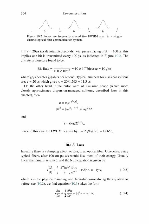
264 Communications
5τ 5τ 5τ
Figure 10.2 Pulses are frequently spaced five FWHM apart in a single-channel optical fiber communication system.
t. If τ = 20 ps (ps denotes picoseconds) with pulse spacing of 5τ = 100 ps, thisimplies one bit is transmitted every 100 ps, as indicated in Figure 10.2. Thebit-rate is therefore found to be:
Bit-Rate =1
100 × 10−12= 10 × 109 bits/sec = 10 gb/s
where gb/s denotes gigabits per second. Typical numbers for classical solitonsare: τ = 20 ps which gives t∗ = 20/1.763 = 11.3 ps.
On the other hand if the pulse were of Gaussian shape (which moreclosely approximates dispersion-managed solitons, described later in thischapter), then
u = u0e−t2/2t2∗ ,
|u|2 = |u0|2e−t2/t2∗ = |u0|2/2,and
t = (log 2)1/2t∗,
hence in this case the FWHM is given by τ = 2√
log 2t∗ = 1.665t∗.
10.1.3 Loss
In reality there is a damping effect, or loss, in an optical fiber. Otherwise, usingtypical fibers, after 100 km pulses would lose most of their energy. Usuallylinear damping is assumed, and the NLS equation is given by
i∂A∂z+
(−k′′(ω)
2
)∂2A∂T 2+ ν|A|2A = −iγA, (10.3)
where γ is the physical damping rate. Non-dimensionalizing the equation asbefore, see (10.2), we find equation (10.3) takes the form
i∂u∂z+
12∂2u∂t2+ |u|2u = −iΓu, (10.4)
10.1 Communications 265
where Γ = γz∗ and, for convenience, we drop the prime from the variables.We can deduce the rate at which the soliton amplitude decays. Multiplying theNLS equation, (10.4), by u∗ and its complex conjugate by u, we find:
iu∗∂u∂z+ u∗
12∂2u∂t2+ |u|4 = −iΓ|u|2
−iu∂u∗
∂z+ u
12∂2u∗
∂t2+ |u|4 = iΓ|u|2.
Noting
∂(uu∗)∂z
= u∗∂u∂z+ u
∂u∗
∂z
and
∂2u∂t2
u∗ − ∂2u∗
∂t2u =
∂
∂t
(u∗∂u∂t− u
∂u∗∂t
),
we get, by substituting the above equations,
i∂|u|2∂z
u∗ +12∂
∂t
(u∗∂u∂t− u
∂u∗∂t
)= −2Γ|u|2,
and hence integrating over the (infinite) domain of the soliton pulse,
∂
∂z
∫ ∞
−∞|u|2 dt = −2Γ
∫ ∞
−∞|u|2 dt. (10.5)
Substituting into (10.5) a classical soliton given by u = η sech(ηt) eiη2z/2,we find
∂
∂z
∫ ∞
−∞η2 sech2(ηt) dt = −2Γ
∫ ∞
−∞η2 sech2(ηt) dt.
This yields the equation governing the change in the soliton parameter,
∂η
∂z= −2Γη.
Thus u = u0e−2Γz and we say the soliton damping rate is 2Γ. This is verydifferent from the rate one would get if one had only a linear equation
i∂u∂z+
12∂2u∂t2= −iΓu,
i.e., if we neglect the nonlinear term in (10.4). In this case, if we takeu= Aeiωt + cc, i.e., we assume a linear periodic wave (sometimes called “CW”
266 Communications
or continuous wave), we find by the same procedure as above, integrating overa period of the linear wave T = 2π/ω:
∂
∂z
∫ 2πω
0|A|2 cos2(ωt) dt = −2Γ
∫ 2πω
0|A|2 cos2(ωt) dt
∂
∂z|A|2 = −2Γ|A|2
∂|A|∂z= −Γ|A|.
Thus for a linear wave (CW): |A| = |A(0)|e−Γz and therefore the amplitude ofa soliton decays at “twice the linear rate”; i.e., a soliton decays at twice thedamping rate as that of a linear (CW) wave.
10.1.4 Amplification
In practice, for sending signals over a long distance, in order to counteractthe damping, the optical field must be amplified. A method, first developed inthe mid-1980s, uses all-optical fibers (typically: “EDFAs”: erbium doped fiberamplifiers)
In order to derive the relevant equation we assume the amplifiers occur atdistinct locations zm = mza, m = 1, 2, . . ., down the fiber and are modeledas Dirac delta functions (G − 1)δ(z − zm), where G is the normalized gain.Here za denotes the normalized amplifier distance: za = �a/z∗, where �a isthe distance between the amplifiers in physical units. The NLS equation takesthe form:
i∂u∂z+
12∂2u∂t2+ |u|2u = i
⎛⎜⎜⎜⎜⎜⎝−Γ +∑m
(G − 1)δ(z − zm)
⎞⎟⎟⎟⎟⎟⎠ u.
This is usually termed a “lumped” model. Integrating from zn− = zn − δ tozn+ = zn + δ, where 0 < δ � 1 and assuming continuity of u and its temporalderivatives
i∫ zn+
zn−
∂u∂z
dz = i∫ zn+
zn−
⎛⎜⎜⎜⎜⎜⎝−Γ +∑m
(G − 1)δ(z − zm)
⎞⎟⎟⎟⎟⎟⎠ u dz
we find
u(zn+, t) − u(zn−, t) = (G − 1)u(zn−, t)
u(zn+, t) = Gu(zn−, t).
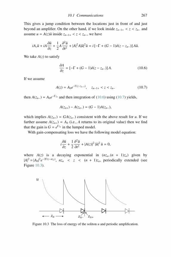
10.1 Communications 267
This gives a jump condition between the locations just in front of and justbeyond an amplifier. On the other hand, if we look inside zn−1+ < z < zn− andassume u = A(z)u inside zn−1+ < z < zn−, we have
iAzu + iA∂u∂z+
12
A∂2u∂t2+ |A|2A|u|2u = i [−Γ + (G − 1)δ(z − zn−)] Au.
We take A(z) to satisfy
∂A∂z= [−Γ + (G − 1)δ(z − zn−)] A. (10.6)
If we assume
A(z) = A0e−Γ(z−zn−1), zn−1+ < z < zn− (10.7)
then A(zn−) = A0e−Γza and then integration of (10.6) using (10.7) yields,
A(zn+) − A(zn−) = (G − 1)A(zn−),
which implies A(zn+) = GA(zn−) consistent with the above result for u. If wefurther assume A(zn+) = A0 (i.e., A returns to its original value) then we findthat the gain is G = eΓza in the lumped model.
With gain-compensating loss we have the following model equation:
i∂u∂z+
12∂2u∂t2+ |A(z)|2 |u|2 u = 0,
where A(z) is a decaying exponential in (nza, (n + 1)za) given by|A|2 = |A0|2e−2Γ(z−nza), nza < z < (n + 1)za, periodically extended (seeFigure 10.3).
u
za zn− zn+
Figure 10.3 The loss of energy of the soliton u and periodic amplification.
268 Communications
In this model u (unlike u) does not have delta functions in the equation anddoes not change discontinuously over one period. We choose |A|2 such that1za
∫ za
0|A|2 dz = 1; hence
1za|A0|2
∫ za
0e−2Γzdz =
|A0|2−2Γza
(e−2Γza − 1) = 1,
|A0|2 = 2Γza
1 − e2Γza.
Note that as za → 0 we have2Γza
1 − e2Γza→ 1.
For notational convenience, we now drop the tilde on u – but stress that the“true” normalized field is u = A(z)u, with A = A0e−Γ(z−zn) where nza < z <(n + 1)za periodically extended. Thus, in summary, our basic gain/loss modelis the “distributed” equation
i∂u∂z+
12∂2u∂t2+ g(z)|u|2u = 0, (10.8)
where g(z) = |A0|2e−2Γ(z−nza), nza < z < (n + 1)za, periodically extended. Noteagain that amplification occurs between zn− < z < zn+. We also see that the
average of g is given by 〈g〉 = 1za
∫ za
0g(z)dz = 1. This is important regarding
multi-scale theory; on average we will see that we get the unperturbed NLSequation, iuz +
12 utt + |u|2u = 0.
10.1.5 Some typical units: Classical solitons
Below we list some typical classical soliton parameter values and useful rela-tionships, where k = 2π/λ and ω/k = c (here, as is standard, k is wave number,ω is frequency etc.):
λ ∼ 1550 nm; c = 3 × 10⁸ m/s; D ∼ 0.5ps
nm · km;
k′′ = −λ2D
2πcps2
km= −0.65
ps2
km; ω = 1.2 × 10¹⁵ rad/s = 193 THz;
τFWHM � 20 ps; t∗ = 11.3 ps; ν =n2ω
4cAeff∼ 2.5
1W · km
; P∗ ∼ 2 mW;
z∗ ∼ 200 km =1νP∗=
1(2.5)(2 × 10⁻³)
=15× 103 = 200 km;
za ∼ 20 km200 km
∼ 0.1; γ = 0.051
km;
γdecibels = 4.343γ = 0.22dbkm
; Γ = γz∗ = 10.
10.2 Multiple-scale analysis of the NLS equation 269
10.2 Multiple-scale analysis of the NLS equation
We begin with (10.8),
i∂u∂z+
12∂2u∂t2+ g(z)|u|2u = 0.
We assume that g(z) is rapidly varying and denote it by g(z) = g(z/za), where0 < za � 1 is the “fast” scale and z∗ ∼ O(1) is the “slow” scale. Recall thatg(z) = A2
0e−2Γ(z−nza), where nza < z < (n + 1)za. Note that in terms of the “fast”scale za, this can be written
g(z) = A20e−2Γza
(z
za−n), n <
zza< (n + 1).
Typically za ∼ 0.1, Γ = 10 and we say that g(z) is rapidly varying on a scaleof length za. Next we assume a solution of the form u = u(ζ,Z, t; ε) whereζ = z/za,Z = z and ε = za as our small parameter. Using
∂
∂z→ ∂
∂Z+
1ε
∂
∂ζ,
we can write the NLS equation as
i
(∂u∂Z+
1ε
∂u∂ζ
)+
12∂2u∂t2+ g(ζ)|u|2u = 0.
Assuming the standard multiple-scale expansion
u = u0 + εu1 + ε2u2 + · · · ,
we find, to leading order, O(1/ε),
i∂u0
∂ζ= 0,
which implies u0 is independent of the fast scale ζ = z/ε; we write u0 = U(z, t).At the next order, O(1), we have
i∂u1
∂ζ+ i
∂u0
∂Z+
12∂2u0
∂t2+ g(ζ)|u0|2u0 = 0,
or
i∂u1
∂ζ= −
(i∂U∂Z+
12∂2U∂t2+ g(ζ)|U |2U
).
Therefore
u1 = i
(i∂U∂Z+
12∂2U∂t2+ 〈g〉|U |2U
)ζ +
∫ ζ
0
(g(ζ) − 〈g〉) dζ |U |2U.
270 Communications
Since g(ζ) is periodic with unit period, g(ζ) = 〈g〉 +∑n�0
gneinζ . We note that
g(ζ) − 〈g〉 has zero mean and hence is non-secular (i.e., it does not grow withζ). The first term, however, will grow without bound, i.e., this term is secular.To remove this secular term, we take, using 〈g〉 = 1,
i∂U∂Z+
12∂2U∂t2+ |U |2U = 0, (10.9)
with u ∼ U to first order, and we see that we regain the lossless NLS equa-tion. This approximation is sometimes called the “guiding center” in solitontheory – see Hasegawa and Kodama (1991a,b, 1995). An alternative multi-scale approach for classical solitons was employed later (Yang and Kath,1997). Equation (10.9) was obtained at the beginning of the classical solitonera. However soon it was understood that noise limited the distance of propa-gation. Explicitly, for typical amplifier models, noise-induced amplitude jitter(Gordon and Haus, 1986) can reduce propagation distance (in units describedearlier) from 10,000 km to about 4000–5000 km. Researchers developed toolsto deal with this problem (see Yang and Kath, 1997), examples being solitontransmission control and the use of filters (see, e.g., Molleneauer and Gordon,2006). But another serious problem was soon encountered. This is describedin the following section.
10.2.1 Multichannel communications: Wavelengthdivision multiplexing
In the mid-1990s communications systems were moving towards multichannelcommunications or “WDM”, standing for wavelength division multiplexing.WDM allows signals to be sent simultaneously in different frequency channels.In terms of the solution of the NLS equation we assume u, for a two-channelsystem, to be initially composed of two soliton solutions in two different chan-nels, u = u1 + u2 that is valid before any interaction occurs. Using classicalsolitons,
uj = η j sech[η j(t −Ω jz)
]eiΩ j t+i
(η2−Ω2
j
)z/2+iφ j ,
with Ω1 � Ω2; usually we take
u2 = sech(t −Ωz) eiΩt+i(1−Ω2)z/2,
u1 = sech(t + Ωz) e−iΩt+i(1−Ω2)z/2,
10.2 Multiple-scale analysis of the NLS equation 271
where for simplicity η1 = η2 = 1, Ω2 = −Ω1 = Ω and we assumeΩ � 1, because in practice the different frequencies are well separated. Onceinteraction begins we assume a solution of the form
u = u1 + u2 + u f , (10.10)
where u f is due to “four-wave mixing” and we assume |u f | � 1 becausesuch four-wave mixing terms generated by the interaction are small. Substi-tuting (10.10) into (10.8) we get
i∂u1
∂z+ i
∂u2
∂z+ i
∂u f
∂z+
12
(∂2u1
∂t2+∂2u2
∂t2+∂2u f
∂t2
)+
+g(z)(u1 + u2 + u f )2(u∗1 + u∗2 + u∗f ) = 0.
Since u1, u2 ∼O(1) and |uf |� 1, we can neglect the terms containing u f .Expanding we arrive at
(u1 + u2 + u f )2(u∗1 + u∗2 + u∗f
)=
= |u1|2u1 + |u2|2u2︸�������������︷︷�������������︸SPM
+ 2|u1|2u2 + 2|u2|2u1︸�����������������︷︷�����������������︸XPM
+ u21u∗2 + u2
2u∗1︸��������︷︷��������︸FWM
+O(u f ),
where SPM means “self-phase modulation”, XPM stands for “cross-phasemodulation” and FWM: “four-wave mixing”. Recall that the frequencies (orfrequency channels) of the solitons uj, j = 1, 2, are given by u1 ∼ e−iΩt andu2 ∼ eiΩt, giving
u21u∗2 ∼ e−3iΩt
u∗1u22 ∼ e+3iΩt.
The equation for the above FWM components (with frequencies ±3iΩt) is
i∂u f
∂z+
12
∂2u f
∂t2+ g(z)
(u2
1u∗2 + u22u∗1)= 0. (10.11)
On the other hand, the equation for u1 (sometimes called channel 1), which isforced by SPM and XPM terms, is
i∂u1
∂z+
12∂2u1
∂t2+ g(z)|u1|2u1 = −2g(z)|u2|2u1. (10.12)
272 Communications
The symmetric analog for channel 2 (u2) is
i∂u2
∂z+
12∂2u2
∂t2+ g(z)|u2|2u2 = −2g(z)|u1|2u2. (10.13)
Since |Ω2 − Ω1| � 1, the equations separate naturally from one another. Thisis most easily understood as separation of energy in Fourier space. Directnumerical simulations support this model.
10.2.2 Four-wave mixing
If we say u f = q + r, where q ∼ e3iΩt and r ∼ e−3iΩt, we can separate (10.11)into two parts:
iqz +12
qtt + g(z)u22u∗1 = 0
irz +12
rtt + g(z)u21u∗2 = 0.
Let us look at the equation for q:
iqz +12
qtt = −g(z)u22u∗1. (10.14)
A similar analysis can be done for r. Note that the right-hand side of (10.14) is
RHS = u22u∗1 = e+3iΩt− i
2Ω2z sech2(t −Ωz) sech(t + Ωz)eiz/2.
It is natural to assume q = F(z, t)e3iΩt−iΩ2z/2, where the rapidly varying phaseis separated out leaving the slowly varying function F(z, t). The equation forF(z, t) then satisfies a linear equation
i(Fz − i
2Ω2F
)+
12
(Ftt + 6iΩFt − 9Ω2F
)= −g(z)R(z, t),
where
R(z, t) = sech2(t −Ωz) sech(t + Ωz)eiz/2.
After simplification, F(z, t) now satisfies
iFz +12
Ftt + 3iΩFt − 4Ω2F = −g(z)R. (10.15)
(We remark that if we put ω f = 3Ω and k f =2Ω2
2 −Ω21
2=Ω2
2, then the phase
of u22u∗1 is ei(ω f t−k f z) and ω2
f /2 − k f = 9Ω2/2 −Ω2/2 = 4Ω2.)
10.2 Multiple-scale analysis of the NLS equation 273
We may now solve (10.15) using Fourier transforms (see also Ablowitzet al., 1996). However, a simple and useful model is obtained by assuming|Ftt |�Ω2F and |ΩFt | � Ω2F. In this case we have the following reducedmodel:
iFz − 4Ω2F = −g(z)R.
Letting R = Reiz/2 leads to
i∂
∂z
(Fe4iΩ2z
)= −g(z)Re4iΩ2z+iz/2. (10.16)
Near the point of collision of the solitons, i.e., at z = 0, there is a non-trivial contribution to F. We consider R as constant in this reduced model.Since g(z) is periodic with period za it can be expanded in a Fourier series,
g(z)=∞∑−∞
gne−2πinz/za , in which case the right-hand side of (10.16) is propor-
tional to
g(z)e4iΩ2z+iz/2 =
∞∑−∞
gneiz[4Ω2−2πn/za+12 ].
Then from (10.16), we see that there is an FWM resonance when
2πnza= 4Ω2 +
12, (10.17)
where n is an integer. We therefore have the growth of FWM termswhenever (10.17) is (nearly) satisfied. Otherwise F can be expected toremain small. Thus, given Ω and za, the nearest integer n is given byn= (4Ω2 + 1/2)za/2π. Using the typical numbers za = 0.1, Ω = 4,
n� (0.1)
(64.56.28
)� 1.03 gives n = 1 as the dominant FWM contribution.
See Figure 10.4 where numerical simulation of (10.1) (with typical param-eters) demonstrates the significant FWM growth for classical solitons. Formore information see Mamyshev and Mollenauer (1996) and Ablowitz et al.(1996).
To avoid the FWM growth/interactions (and noise effects) that createdsignificant penalties, researchers began to use “dispersion-management”described in the following section. Dispersion-management (DM) is character-ized by large varying local dispersion that changes sign. With such large localdispersion variation one expects strongly reduced FWM contribution, whichhas been analyzed in detail (see Ablowitz et al., 2003a).
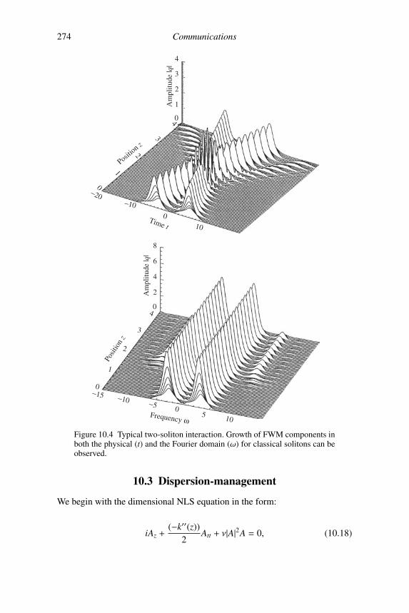
274 Communications
Am
plitu
de |q
|
Am
plitu
de |q
|
4
3
2
1
04
3
2
1
0
Position z
Posit
ion
z
−20
−15 −10 −5 0
0
1
2
3
4
Frequency ω5 10
−10
010
Time t
0
2
4
6
8
Figure 10.4 Typical two-soliton interaction. Growth of FWM components inboth the physical (t) and the Fourier domain (ω) for classical solitons can beobserved.
10.3 Dispersion-management
We begin with the dimensional NLS equation in the form:
iAz +(−k′′(z))
2Att + ν|A|2A = 0, (10.18)
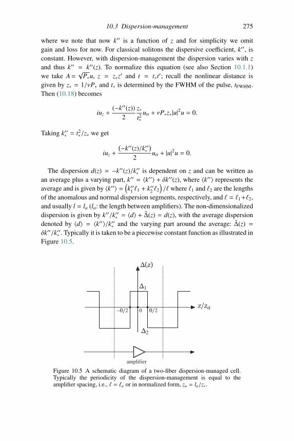
10.3 Dispersion-management 275
where we note that now k′′ is a function of z and for simplicity we omitgain and loss for now. For classical solitons the dispersive coefficient, k′′, isconstant. However, with dispersion-management the dispersion varies with zand thus k′′ = k′′(z). To normalize this equation (see also Section 10.1.1)we take A=
√P∗u, z = z∗z′ and t = t∗t′; recall the nonlinear distance is
given by z∗ = 1/νP∗ and t∗ is determined by the FWHM of the pulse, tFWHM.Then (10.18) becomes
iuz +(−k′′(z))
2z∗t2∗
utt + νP∗z∗|u|2u = 0.
Taking k′′∗ = t2∗/z∗ we get
iuz +
(−k′′(z)/k′′∗)
2utt + |u|2u = 0.
The dispersion d(z) = −k′′(z)/k′′∗ is dependent on z and can be written asan average plus a varying part, k′′ = 〈k′′〉 + δk′′(z), where 〈k′′〉 represents theaverage and is given by 〈k′′〉 =
(k′′1 �1 + k′′2 �2
)/� where �1 and �2 are the lengths
of the anomalous and normal dispersion segments, respectively, and � = �1+�2,and usually l = la (la: the length between amplifiers). The non-dimensionalizeddispersion is given by k′′/k′′∗ = 〈d〉 + Δ(z) = d(z), with the average dispersiondenoted by 〈d〉 = 〈k′′〉/k′′∗ and the varying part around the average: Δ(z) =δk′′/k′′∗ . Typically it is taken to be a piecewise constant function as illustrated inFigure 10.5.
Δ(z)
θ/2
amplifier
0z/za−θ/2
Δ2
Δ1
Figure 10.5 A schematic diagram of a two-fiber dispersion-managed cell.Typically the periodicity of the dispersion-management is equal to theamplifier spacing, i.e., � = �a or in normalized form, za = la/z∗.
276 Communications
The non-dimensionalized NLS equation is now
iuz +d(z)
2utt + |u|2u = 0.
Damping and amplification can be added, as before, which leads to ourfundamental model:
iuz +d(z)
2utt + g(z)|u|2u = 0. (10.19)
If d(z) does not change sign, we can simplify (10.19) by letting
z(z) =∫ z
0h(z′) dz′
so that ∂z = h(z)∂z, where h(z) is to be determined. Equation (10.19) thenbecomes
iuz +12
d(z)h(z)
utt +g(z)h(z)|u|2u = 0.
If fibers could be constructed so that h(z) = d(z) = g(z), then we would obtainthe classical NLS equation:
iuz +12
utt + |u|2u = 0.
This type of fiber is called “dispersion following the loss profile”.Unfortunately, it is very difficult to manufacture such fibers. An idea first
suggested in 1980 (Lin et al., 1980) that has become standard technology isto fuse together fibers that have large and different, but (nearly) constant, dis-persion characteristics. A two-step “dispersion-managed” transmission line ismodeled as follows:
d(z) = 〈d〉 + Δ(z/za)za
, 〈Δ〉 =∫ 1
0Δ(ζ) dζ = 0, ζ =
zza.
We quantify the parameters of a two-step map as illustrated in Figure 10.5. Thevariation of the dispersion is given by Δ(ζ),
Δ(ζ) =
⎧⎪⎪⎨⎪⎪⎩Δ1, 0 ≤ |ζ | < θ/2,Δ2, θ/2 < |ζ | < 1/2.
10.4 Multiple-scale analysis of DM 277
In this two-step map we usually parameterize Δ j, j = 1, 2, by
Δ1 =2sθ, Δ2 =
−2s1 − θ ,
where 〈Δ〉 = 0 and s is termed the map strength parameter, defined as
s =θΔ1 − (1 − θ)Δ2
4=
area enclosed byΔ4
. (10.20)
Note that 〈Δ〉 = θΔ1 + (1 − θ)Δ2 = 0, as it should be by its definition.Remarkably dispersion-management is also an important technology that is
used to produce ultra-short pulses in mode-locked lasers, such as in Ti:sapphirelasers (Ablowitz et al., 2004a; Quraishi et al., 2005; Ablowitz et al., 2008)discussed in the next chapter.
10.4 Multiple-scale analysis of DM
In this section we apply the method of multiple scales to (10.19) (see Ablowitzand Biondini, 1998):
iuz +12
(〈d〉 + Δ(ζ)
za
)utt + g(ζ)|u|2u = 0. (10.21)
In (10.21), let us call our small parameter za = ε, assume za ≡ ε � 1,
and define u = u(t, ζ,Z; ε), ζ = z/ε, and Z = z; hence,∂
∂z=
1ε
∂
∂ζ+
∂
∂Z.
Thus,
1ε
(i∂u∂ζ+
12Δ(ζ)
∂2u∂t2
)+ i
∂u∂Z+
12〈d〉 ∂
2u∂t2+ g(ζ)|u|2u = 0.
With a standard multiple-scales expansion u = u0 + εu1 + ε2u2 + · · · , we have
at leading order, O (1/ε),
i∂u0
∂ζ+Δ(ζ)
2∂2u0
∂t2= 0. (10.22)
We solve (10.22) using Fourier transforms, defined by (inverse transform)
u0(t, ζ,Z) ≡ 12π
∫ ∞
−∞u0(ω, ζ, Z)eiωt dω,
and (direct transform)
u0(ω, ζ, Z) = F {u0} ≡∫ ∞
−∞u0(t, ζ,Z)e−iωt dt.
278 Communications
Taking the Fourier transform of (10.22) and solving the resulting ODE,we find
∂u0
∂ζ− ω
2
2Δ(ζ)u0 = 0, (10.23a)
u0(ω, ζ, Z) = U(ω, Z)e−iω2C(ζ)/2, (10.23b)
where C(ζ) =∫ ζ
0Δ(ζ′) dζ′ is the integrated dispersion.
At the next order, O(1), we have
i∂u1
∂ζ+Δ(ζ)
2∂2u1
∂t2= F1, (10.24)
where
−F1 ≡ i∂u0
∂Z+
12〈d〉 ∂
2u0
∂t2+ g(ζ)|u0|2u0.
Again using the Fourier transform, (10.24) becomes
iu1ζ − ω2
2Δ(ζ)u1 = F1,
or
i∂
∂ζ
(u1eiω2C(ζ)/2
)= F1eiω2C(ζ)/2.
Hence [iu1eiω2C(ζ)/2
]ζ′=ζζ′=0=
∫ ζ
0F1eiω2C(ζ)/2 dζ.
Since C(ζ) is periodic in ζ and Δ has zero mean, u0 is also periodic in ζ. There-fore to remove secular terms we must have
⟨F1eiω2C(ζ)/2
⟩= 0. Thus we require
that ⟨F1eiω2C(ζ)/2
⟩=
∫ 1
0F1eiω2C(ζ)/2 dζ = 0,
or ∫ 1
0
(i∂u0
∂Z− 〈d〉
2ω2u0
)eiω2C(ζ)/2 dζ
+
∫ 1
0g(ζ)F
{|u0|2u0
}eiω2C(ζ)/2 dζ = 0.
Using (10.23b) we get the dispersion-managed NLS (DMNLS) equation:
i∂U∂Z− 〈d〉
2ω2U +
⟨g(ζ)F
{|u0|2 u0
}eiω2C(ζ)/2
⟩= 0. (10.25)
10.4 Multiple-scale analysis of DM 279
10.4.1 The DMNLS equation in convolution form
Equation (10.25) is useful numerically, but analytically it is often better totransform the nonlinear term to Fourier space. Using the Fourier transform
u0(t, ζ,Z) =1
2π
∫ ∞
−∞U(ω, Z)e−iω2C(ζ)/2eiωt dω (10.26)
in the nonlinear term in (10.25), we find, after interchanging integrals (seeSection 10.4.2 for a detailed discussion):
⟨g(ζ)F [|u0|2 u0]eiω2C(ζ)/2
⟩=
∫ ∞
−∞
∫ ∞
−∞r(ω1ω2)U(ω + ω1, z)
× U(ω + ω2, z)U∗(ω + ω1 + ω2, z) dω1dω2,
(10.27)
where
r(ω1ω2) =1
(2π)2
∫ 1
0g(ζ) exp
[iω1ω2C(ζ)
]dζ. (10.28)
If g(z) = 1, i.e., the lossless case, we find for the two-step map, depicted inFigure 10.5, that
r(x) =sin sx
(2π)2sx, (10.29)
where s is called the DM map strength [see (10.20)]. This leads to anotherrepresentation of the DMNLS equation in “convolution form”
iUZ − 〈d〉2 ω2U +∫ ∞
−∞
∫ ∞
−∞r(ω1ω2)U(ω + ω1, z)U(ω + ω2, z)
U∗(ω + ω1 + ω2, z) dω1 dω2 = 0, (10.30)
where r(ω1ω2) is given in (10.28) (Ablowitz and Biondini, 1998; Gabitov andTuritsyn, 1996).
The above DMNLS equation has a natural dual in the time domain. Tak-ing the inverse Fourier transform of (10.30) yields (see Section 10.4.2 fordetails)
iUZ +〈d〉2
Utt +
∫ ∞
−∞
∫ ∞
−∞R(t1, t2)U(t1)U(t2)U∗(t1 + t2 − t) dt1dt2 = 0,
(10.31)
280 Communications
where
R(t1, t2) =∫ ∞
−∞
∫ ∞
−∞r(ω1ω2)eiω1t2 eiω2t1 dω1 dω2.
Note that if Δ(z) → 0, we recover the classical NLS equation since it canbe shown that as s → 0, r → 1/(2π)2, R(t1, t2) → δ(t1)δ(t2), recalling thatδ(t) = 1
2π
∫eiωt dt. When g(z) = 1, the lossless case, we also find
R(t1, t2) =1
2πsCi
( |t1t2|s
)with
Ci(x) =∫ ∞
x
cos uu
du.
10.4.2 Detailed derivation
In this subsection we provide the details underlying the derivation of (10.27)and (10.31) as well as the special cases of (10.29) when g = 1. We start bywriting (10.27) explicitly:
I(ω) = I ≡⟨g(ζ)F
{|u0|2 u0
}eiω2C(ζ)/2
⟩=
∫ 1
0g(ζ)
∫ ∞
−∞dt
[1
2π
∫ ∞
−∞U(ω1,Z)e−iω2
1C(ζ)/2eiω1t dω1
]×[
12π
∫ ∞
−∞U(ω2,Z)e−iω2
2C(ζ)/2eiω2t dω2
]×[
12π
∫ ∞
−∞U∗(ω3,Z)eiω2
3C(ζ)/2e−iω3t dω3
]× e−iωteiω2C(ζ)/2 dζ.
Interchanging the order of integration and grouping the exponentials together,
I =∫ 1
0g(ζ)
∫ ∞
−∞
∫ ∞
−∞
∫ ∞
−∞
(1
2π
)2U(ω1,Z)U(ω2,Z)
× U∗(ω3,Z)e−i(ω21+ω
22−ω2
3−ω2)C(ζ)/2
× 12π
∫ ∞
−∞ei(ω1+ω2−ω3−ω)t dt dω1 dω2dω3 dζ.
Recall that the Dirac delta function can be written as
δ(ω′ − ω) =1
2π
∫ ∞
−∞ei(ω′−ω)t dt,
10.4 Multiple-scale analysis of DM 281
where ω′ = ω1 + ω2 − ω3. Thus, with ω3 = ω1 + ω2 − ω,
I =∫ 1
0g(ζ)
∫ ∞
−∞
∫ ∞
−∞
(1
2π
)2U(ω1,Z)U(ω2,Z)U∗(ω1 + ω2 − ω, Z)
× exp[−i((ω1 + ω2)ω − ω1ω2 − ω2
)C(ζ)
]dω1 dω2 dζ. (10.32)
A more symmetric form is obtained when we use
ω1 = ω + ω1
ω2 = ω + ω2
}⇒ ω1 + ω2 − ω = ω1 + ω2 + ω.
Note that −ω1ω2 + (ω1 + ω2)ω= − (ω+ ω1)(ω+ ω2)+ (ω1 + ω2 + ω)ω =−ω1ω2. Equation (10.32) can now be written, after dropping thetildes,
I =∫ 1
0g(ζ)
∫ ∞
−∞
∫ ∞
−∞U(ω1 + ω,Z)U(ω2 + ω,Z)
× U∗(ω1 + ω2 + ω,Z)
(1
2π
)2eiω1ω2C(ζ) dω1 dω2 dζ. (10.33)
We now define the DMNLS kernel r:
r(x) ≡ 1(2π)2
∫ 1
0g(ζ)eixC(ζ) dζ.
Then (10.33) becomes
I =∫ ∞
−∞
∫ ∞
−∞r(ω1ω2)U(ω1 + ω,Z)
× U(ω2 + ω,Z)U∗(ω1 + ω2 + ω, Z) dω1 dω2,
which is the third term in (10.30), i.e., (10.27).For the lossless case, i.e., g(ζ) = 1 and a two-step map, r(x), the analysis
can be considerably simplified. We now give details of this calculation. First,for a two-step map with C(0) = 0
C(ζ) =∫ ζ
0Δ(ζ′) dζ′ =
⎧⎪⎪⎪⎪⎪⎨⎪⎪⎪⎪⎪⎩Δ1ζ, 0 < ζ < θ/2
Δ2ζ +C1, θ/2 < ζ < 1 − θ/2Δ1ζ +C2, 1 − θ/2 < ζ < 1
C1 = Δ1θ/2 − Δ2θ/2 = (Δ1 − Δ2)θ/2
C2 = −Δ1,
282 Communications
where C1,2 are obtained by requiring continuity at ζ = θ/2, 1−θ/2, respectively.Recall that since 〈Δ〉 = 0, we have Δ1θ + Δ2(1 − θ) = 0. Thus,
I =∫ 1
0eixC(ζ) dζ
=
∫ θ/2
0eiΔ1ζx dζ +
∫ 1−θ/2
θ/2ei(Δ2ζ+C1)x dζ +
∫ 1
1−θ/2ei(Δ1ζ+C2)x dζ
I =eiΔ1θx/2 − 1
iΔ1x
+ eiC1 x
[eiΔ2(1−θ/2)x − eiΔ2θx/2
iΔ2x
]+ eiC2 x
[eiΔ1 x − eiΔ1(1−θ/2)x
iΔ1x
].
Using C1 = (Δ1 − Δ2)θ/2 and C2 + Δ1 = 0,
I =eiΔ1θx/2−e−iΔ1θ/2
iΔ1x+
ei(Δ2(1−θ/2)x+(Δ1−Δ2)θ/2)−ei(Δ2θx/2+(Δ1−Δ2)θ/2)
iΔ2x
I =eiΔ1(θ/2)x − e−iΔ1(θ/2)x
iΔ1x+
eiΔ2(1−θ)x+Δ1θ/2 − e−iΔ1(θ/2)x
iΔ2x.
Then using Δ2(1 − θ) = −Δ1θ, we get
I =eiΔ1(θ/2)x − e−iΔ1(θ/2)x
iΔ1x− eiΔ1(θ/2)x − e−iΔ1(θ/2)x
iΔ2x.
Setting s =Δ1θ − (1 − θ)Δ2
4, we have s =
Δ1θ
2and hence∫ 1
0eiC(ζ)x dζ =
1ix
[I =
eisx − e−isx
Δ1− eisx − e−isx
Δ2
]=
2 sin sxx
(1Δ1− 1Δ2
)=
2 sin sxx
(1Δ1+
1 − θθΔ1
)=
2 sin sxΔ1θx
=sin sx
sx;
thus when g = 1 ∫ 1
0eiC(ζ)x dζ =
sin sxsx
. (10.34)
Next we investigate the inverse Fourier transform of (10.30). Using
U =1
2π
∫ ∞
−∞Ueiωt dω
10.4 Multiple-scale analysis of DM 283
and taking the inverse Fourier transform of (10.30) gives
iUZ +〈d〉2
Utt + F −1⟨gF{|u0|2 u0
}eiω2C(ζ)/2
⟩= 0.
Now,
F −1⟨gF{|u0|2 u0
}eiω2C(ζ)/2
⟩=
∫ ∞
−∞eiωt
[∫ ∞
−∞
∫ ∞
−∞r(ω1ω2)U(ω1 + ω,Z)U(ω2 + ω, Z)
× U∗(ω1 + ω2 + ω,Z) dω1dω2
]dω
=
∫ ∞
−∞eiωt∫ ∞
−∞
∫ ∞
−∞r(ω1ω2)
[∫ ∞
−∞U(t1)e−i(ω1+ω)t1 dt1
]×[∫ ∞
−∞U(t2)e−i(ω2+ω)t2 dt2
]×[∫ ∞
−∞U∗(t3)ei(ω1+ω2+ω)t3 dt3
]dω1 dω2dω
=
∫ ∞
−∞
∫ ∞
−∞dω1dω2r(ω1ω2)
∫ ∞
−∞dt1U(t1) dt2
∫ ∞
−∞U(t2) dt3
×∫ ∞
−∞U∗(t3)eiω1(t3−t1)eiω2(t3−t2) 1
2π
∫ ∞
−∞eiω(t−t1−t2+t3) dω︸������������������������︷︷������������������������︸
use δ(t−t1−t2+t3)
=
∫ ∞
−∞
∫ ∞
−∞dω1dω2r(ω1ω2)
×∫ ∞
−∞
∫ ∞
−∞dt1 dt2U(t1)eiω1(t2−t)U(t2)eiω2(t1−t)U∗(t1 + t2 − t).
Thus,
F −1⟨gF{|u0|2 u0
}eiω2C(ζ)/2
⟩=
∫ ∞
−∞
∫ ∞
−∞R(t1, t2)U(t1)U(t2)U∗(t1 + t2 − t) dt1 dt2,
where
R(t1, t2) ≡∫ ∞
−∞
∫ ∞
−∞r(ω1ω2)eiω1(t2−t)eiω2(t1−t) dω1 dω2.
284 Communications
With t1 = t1 + t and t2 = t2 + t (and dropping the ∼) we have,
F −1⟨gF{|u0|2 u0
}eiω2C(ζ)/2
⟩=
∫ ∞
−∞
∫ ∞
−∞R(t1, t2)U(t + t1)U(t + t2)U∗(t + t1 + t2) dt1 dt2,
and
R(t1, t2) =∫ ∞
−∞
∫ ∞
−∞r(ω1ω2)eiω1t1+iω2t2 dω1 dω2, (10.35)
the last equality being obtained by interchanging the roles of ω1 and ω2, i.e.,ω1 → ω2 and ω2 → ω1.
The expression for R(t1, t2) can also be further simplified when g(ζ) = 1.From (10.34) and (10.35),
R(t1, t2) =1
(2π)2
∫ ∞
−∞
∫ ∞
−∞sin sω1ω2
sω1ω2eiω1t1+iω2t2 dω1 dω2.
Letting, ω1 = u1/t1, ω2 = u2/t2
R(t1, t2) =1
(2π)2
∫ ∞
−∞
∫ ∞
−∞sgn t1 sgn t2︸��������︷︷��������︸
sgn(t1t2)
sin(
su1u2t1t2
)su1u2
eiu1+iu2 du1 du2
=1
(2π)2s
∫ ∞
−∞
∫ ∞
−∞
sin(
u1u2γ
)u1u2
eiu1+iu2 du1 du2,
where γ =∣∣∣∣ t1t2
s
∣∣∣∣. Then
R(t1, t2) =1
(2π)2s
∫ ∞
−∞
∫ ∞
−∞
(eiu1u2/γ − e−iu1u2/γ
)2iu1u2
ei(u1+u2) du1 du2,
=1
2is(2π)2
∫ ∞
−∞
∫ ∞
−∞eiu1
u1
(eiu2(u1/γ+1) − e−iu2(u1/γ−1)
)u2
du1 du2.
Let us look at the second integral:
I =∫ ∞
−∞
(eiu2(u1/γ+1) − e−iu2(u1/γ−1)
)u2
du2.
Denoting the two terms as I1 and I2, respectively, and using contour integrationyields
I1 = −∫ ∞
−∞eiu2(u1/γ+1)
u2du2 = +iπ sgn
(u1
γ+ 1)
I2 = −∫ ∞
−∞eiu2(1−u1/γ)
u2du2 = +iπ sgn
(1 − u1
γ
),
10.4 Multiple-scale analysis of DM 285
where −∫ ∞−∞ denotes the Cauchy principal value integral. Thus we have
R(t1, t2) =iπ
2is (2π)2
∫ ∞
−∞eiu1
u1
[sgn
(u1
γ+ 1
)− sgn
(1 − u1
γ
)]du1
=1
(4πs) · 2[(−∫ ∞
−γeiu1
u1du1 − −
∫ −γ
−∞eiu1
u1du1
)−(−∫ γ
−∞eiu1
u1du1 − −
∫ ∞
γ
eiu1
u1du1
)]=
1(4πs) · 2
[−−∫ −γ
−∞e−iu1
u1du1 − −
∫ −γ
−∞eiu1
u1du1
+ −∫ ∞
γ
eiu1
u1du1 + −
∫ ∞
γ
e−iu1
u1du1
]=
14πs
[∫ ∞
γ
cos u1
u1du1 −
∫ −γ
−∞cos u1
u1du1
]=
12πs
∫ ∞
γ
cos u1
u1du1
=1
2πs
∫ ∞
1
cos γyy
dy ≡ 12πs
Ci
( |t1t2|s
).
where we used γ =∣∣∣∣∣ t1t2
s
∣∣∣∣∣.10.4.3 Dispersion-managed solitons
DM solitons are stationary solutions of the DMNLS equation, (10.30). We nowlook for solutions of the form
U(ω, Z) = eiλ2Z/2F(ω),
where the only z-dependence is a linearly evolving phase. With this substitu-tion, (10.30) becomes(
λ2 + 〈d〉ω2
2
)F(ω) −
∫ ∞
−∞
∫ ∞
−∞r(ω1ω2)F(ω + ω1)
× F(ω + ω2)F∗(ω + ω1 + ω2) dω1 dω2 = 0
or
F(ω) = − 2λ2 + 〈d〉ω2
∫ ∞
−∞
∫ ∞
−∞r(ω1ω2)F(ω + ω1)
× F(ω + ω2)F∗(ω + ω1 + ω2) dω1 dω2. (10.36)
286 Communications
Thus we wish to find fixed points of the integral equation (10.36). When r(x) isnot constant, obtaining closed-form solutions of this nonlinear integral equa-tion is difficult. However we can readily obtain numerical solutions for 〈d〉 > 0.Ablowitz and Biondini (1998) obtained numerical solutions using a fixed pointiteration technique similar to that originally introduced by Petviashvili (1976).Below we first discuss a modification of this method called spectral renormal-ization, which has proven to be useful in a variety of nonlinear problems whereobtaining localized solutions are of interest.
As we discussed earlier, another formulation of the non-local term is∫ ∞
−∞
∫ ∞
−∞r(ω1ω2)F(ω + ω1)F(ω + ω2)F∗(ω + ω1 + ω2) dω1 dω2 =
=⟨g(z)F
{|u0|2 u0
}eiω2C(ζ)/2 − iλ2Z/2
⟩which is useful in the numerical schemes mentioned below. It should also benoted from the multiple-scales perturbation expansion, that u0 is obtained bythe inverse Fourier transform of
u0(ω, ζ, Z) = F(ω)eiλ2Z/2e−iω2C(ζ)/2.
The naive iteration procedure is given by
F(m+1)(ω) =2
λ2 + 〈d〉ω2
⟨g(z)F
{|u0|2 u0
}(m)eiω2C(ζ)/2−iλ2Z/2
⟩≡ Im[F],
(10.37)
where m = 0, 1, 2, . . . and u(m)0 = Fm(ω)e−iω2C(ζ)/2. At m = 0, F(0)(ω) is taken
to be the inverse Fourier transform of a Gaussian or “sech”-type function.However, if we iterate (10.37) directly, the iteration generally diverges so werenormalize as follows.
In (10.37) we substitute F = μG. We then find the following iterationequations
Gn+1 = μ2nI[Gn]
with
μ2n =
(Gn, Gn)
(Gn, I[Gn])
where (Gn, In) ≡ ∫ G∗n, In
)dω and G0(t) can be a localized function, i.e., Gaus-
sian or sech profile. In either case, the iterations converge rapidly. More detailscan be found in Ablowitz and Musslimani (2005) and Ablowitz and Horikis(2009a).
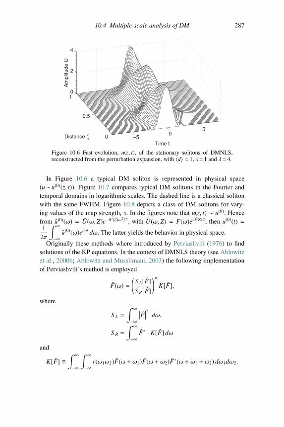
10.4 Multiple-scale analysis of DM 287
−50
50
0.5
10
2
4
Time tDistance ζ
Am
plitu
de U
Figure 10.6 Fast evolution, u(z, t), of the stationary solitons of DMNLS,reconstructed from the perturbation expansion, with 〈d〉 = 1, s= 1 and λ= 4.
In Figure 10.6 a typical DM soliton is represented in physical space(u∼ u(0)(z, t)). Figure 10.7 compares typical DM solitons in the Fourier andtemporal domains in logarithmic scales. The dashed line is a classical solitonwith the same FWHM. Figure 10.8 depicts a class of DM solitons for vary-ing values of the map strength, s. In the figures note that u(z, t) ∼ u(0). Hencefrom u(0)(ω) = U(ω, Z)e−iC(ζ)ω2/2, with U(ω, Z) = F(ω)eiλ2Z/2, then u(0)(t) =1
2π
∫ ∞
−∞u(0)(ω)eiωt dω. The latter yields the behavior in physical space.
Originally these methods where introduced by Petviashvili (1976) to findsolutions of the KP equations. In the context of DMNLS theory (see Ablowitzet al., 2000b; Ablowitz and Musslimani, 2003) the following implementationof Petviashvili’s method is employed
F(ω) =
(S L[F]
S R[F]
)p
K[F],
where
S L =
∫ ∞
−∞
∣∣∣F∣∣∣2 dω,
S R =
∫ ∞
−∞F∗ · K[F] dω
and
K[F] ≡∫ ∞
−∞
∫ ∞
−∞r(ω1ω2)F(ω + ω1)F(ω + ω2)F∗(ω + ω1 + ω2) dω1dω2.
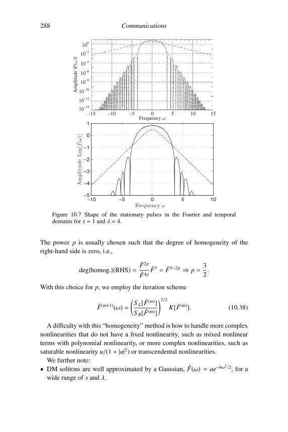
288 Communications
100
10–2
10–4
10–6A
mpl
itude
|F(ω
)|10–8
10–10
10–12
10–14
–15 –10 –5 0Frequency ω
5 10 15
−10 −5 0 5 10−5
−4
−3
−2
−1
0
1
Frequency
Am
plit
ude
Log
[f(ω
)]
ω
Figure 10.7 Shape of the stationary pulses in the Fourier and temporaldomains for s = 1 and λ = 4.
The power p is usually chosen such that the degree of homogeneity of theright-hand side is zero, i.e.,
deg{homog.}(RHS) =F2p
F4pF3 = F3−2p ⇒ p =
32.
With this choice for p, we employ the iteration scheme
F(m+1)(ω) =
(S L[F(m)]
S R[F(m)]
)3/2K[F(m)]. (10.38)
A difficulty with this “homogeneity” method is how to handle more complexnonlinearities that do not have a fixed nonlinearity, such as mixed nonlinearterms with polynomial nonlinearity, or more complex nonlinearities, such assaturable nonlinearity u/(1 + |u|2) or transcendental nonlinearities.
We further note:• DM solitons are well approximated by a Gaussian, F(ω) � ae−bω2/2, for a
wide range of s and λ.
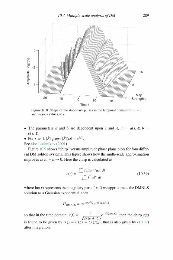
10.4 Multiple-scale analysis of DM 289
−20 −10 0 10 200
8
16
−4
−2
0
MapStrength s
Time t
Am
plitu
de L
og[f(
t)]
Figure 10.8 Shape of the stationary pulses in the temporal domain for λ = 1and various values of s.
• The parameters a and b are dependent upon s and λ, a = a(s, λ), b =b(s, λ).
• For s � 1, |F| grows |F|(ω) ∼ s1/2.See also Lushnikov (2001).
Figure 10.9 shows “chirp” versus amplitude phase plane plots for four differ-ent DM soliton systems. This figure shows how the multi-scale approximationimproves as za = ε→ 0. Here the chirp is calculated as
c(z) =
∫ ∞−∞ t Im {u∗ut} dt∫ ∞−∞ t2 |u|2 dt
, (10.39)
where Im(x) represents the imaginary part of x. If we approximate the DMNLSsolution as a Gaussian exponential, then
UDMNLS = ae−bω2/2e−iC(ζ)ω2/2,
so that in the time domain, u(t) =a√
2π(b + iC)e−t2/2(b+iC), then the chirp c(z)
is found to be given by c(z) = C(ζ) = C(z/za); that is also given by (10.39)after integration.
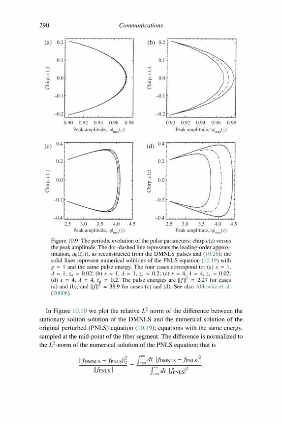
290 Communications
0.2
0.1
0.0
–0.1
–0.2
0.90
2.5–0.4
–0.2
0.0
Chi
rp, c
(z)
Chi
rp, c
(z)
0.2
0.1
0.0
–0.1
–0.2
Chi
rp, c
(z)
0.2
0.4(c)
–0.4
–0.2
0.0
Chi
rp, c
(z)
0.2
0.4(d)
(a) (b)
3.0 3.5 4.0 4.5
0.92 0.94 0.96 0.98Peak amplitude, |q|max(z)
0.90 0.92 0.94 0.96 0.98Peak amplitude, |q|max(z)
Peak amplitude, |q|max(z)2.5 3.0 3.5 4.0 4.5
Peak amplitude, |q|max(z)
Figure 10.9 The periodic evolution of the pulse parameters: chirp c(z) versusthe peak amplitude. The dot–dashed line represents the leading-order approx-imation, u0(ζ, t), as reconstructed from the DMNLS pulses and (10.26); thesolid lines represent numerical solitions of the PNLS equation (10.19) withg = 1 and the same pulse energy. The four cases correspond to: (a) s = 1,λ = 1, za = 0.02; (b) s = 1, λ = 1, za = 0.2; (c) s = 4, λ = 4, za = 0.02;(d) s = 4, λ = 4, za = 0.2. The pulse energies are ‖ f ‖2 = 2.27 for cases(a) and (b), and ‖ f ‖2 = 38.9 for cases (c) and (d). See also Ablowitz et al.(2000b).
In Figure 10.10 we plot the relative L2 norm of the difference between thestationary soliton solution of the DMNLS and the numerical solution of theoriginal perturbed (PNLS) equation (10.19); equations with the same energy,sampled at the mid-point of the fiber segment. The difference is normalized tothe L2-norm of the numerical solution of the PNLS equation; that is
‖ fDMNLS − fPNLS‖22‖ fPNLS‖ =
∫ ∞−∞ dt | fDMNLS − fPNLS|2∫ ∞
−∞ dt | fPNLS|2.
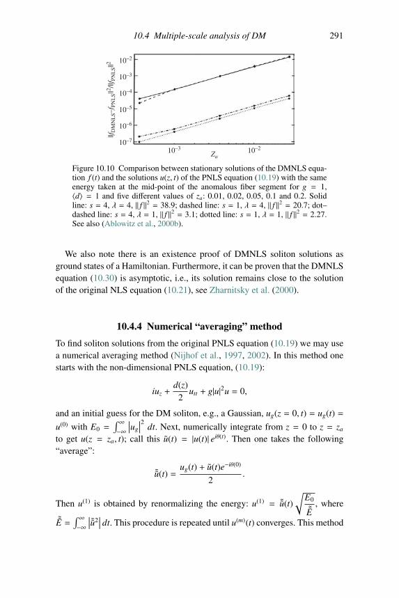
10.4 Multiple-scale analysis of DM 291
10–2
10–3
10–4
10–5
10–6
||fD
MN
LS–
f PN
LS|
|2 /||f P
NL
S||2
10–7
10–3 10–2Za
Figure 10.10 Comparison between stationary solutions of the DMNLS equa-tion f (t) and the solutions u(z, t) of the PNLS equation (10.19) with the sameenergy taken at the mid-point of the anomalous fiber segment for g = 1,〈d〉 = 1 and five different values of za: 0.01, 0.02, 0.05, 0.1 and 0.2. Solidline: s = 4, λ = 4, ‖ f ‖2 = 38.9; dashed line: s = 1, λ = 4, ‖ f ‖2 = 20.7; dot–dashed line: s = 4, λ = 1, ‖ f ‖2 = 3.1; dotted line: s = 1, λ = 1, ‖ f ‖2 = 2.27.See also (Ablowitz et al., 2000b).
We also note there is an existence proof of DMNLS soliton solutions asground states of a Hamiltonian. Furthermore, it can be proven that the DMNLSequation (10.30) is asymptotic, i.e., its solution remains close to the solutionof the original NLS equation (10.21), see Zharnitsky et al. (2000).
10.4.4 Numerical “averaging” method
To find soliton solutions from the original PNLS equation (10.19) we may usea numerical averaging method (Nijhof et al., 1997, 2002). In this method onestarts with the non-dimensional PNLS equation, (10.19):
iuz +d(z)
2utt + g|u|2u = 0,
and an initial guess for the DM soliton, e.g., a Gaussian, ug(z = 0, t) = ug(t) =
u(0) with E0 =∫ ∞−∞∣∣∣ug
∣∣∣2 dt. Next, numerically integrate from z = 0 to z = za
to get u(z = za, t); call this u(t) = |u(t)| eiθ(t). Then one takes the following“average”:
˜u(t) =ug(t) + u(t)e−iθ(0)
2.
Then u(1) is obtained by renormalizing the energy: u(1) = ˜u(t)
√E0
˜E, where
˜E =∫ ∞−∞∣∣∣ ˜u2∣∣∣ dt. This procedure is repeated until u(m)(t) converges. This method
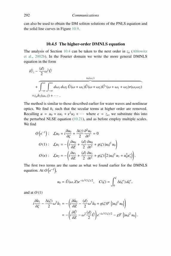
292 Communications
can also be used to obtain the DM soliton solutions of the PNLS equation andthe solid line curves in Figure 10.9.
10.4.5 The higher-order DMNLS equation
The analysis of Section 10.4 can be taken to the next order in za (Ablowitzet al., 2002b). In the Fourier domain we write the more general DMNLSequation in the form
iUz − 〈d〉2 ω2U
+
n0(ω,z)︷����������������������������������������������������������������������������������︸︸����������������������������������������������������������������������������������︷∫ ∞
−∞
∫ ∞
−∞dω1 dω2 U(ω + ω1)U(ω + ω2)U∗(ω + ω1 + ω2)r(ω1ω2)
=zan1(ω, z) + · · · .The method is similar to those described earlier for water waves and nonlinearoptics. We find n1 such that the secular terms at higher order are removed.Recalling u = u0 + εu1 + ε
2u2 + · · · where ε = za, we substitute this intothe perturbed NLSE equation (10.21), and as before employ multiple scales.We find
O(ε−1)
: Lu0 = i∂u0
∂ζ+Δ(z)
2∂2u0
∂t2= 0
O (1) : Lu1 = −(i∂u0
∂Z+〈d〉2∂u0
∂t2+ g(ζ) |u0|2 u0
)O (ε) : Lu2 = −
(i∂u1
∂Z+〈d〉2∂u1
∂t2+ g(ζ)
(2 |u0|2 u1 + u2
0u∗1)).
The first two terms are the same as what we found earlier for the DMNLSequation. At O
(ε−1),
u0 = U(ω, Z)e−iω2C(ζ)/2, C(ζ) =∫ ζ
0Δ(ζ′) dζ′,
and at O (1)
i∂u1
∂ζ− Δ(ζ)
2ω2u1 = −
(i∂u0
∂Z− 〈d〉
2ω2u0 + g(ζ)F
{|u0|2 u0
})= −
(i∂U∂Z− ω2 〈d〉
2U
)e−iω2C(ζ)/2 − gF
{|u0|2 u0
}.
10.4 Multiple-scale analysis of DM 293
Thus,
∂
∂ζ
(iu1eiC(ζ)ω2/2
)= −
(i∂U∂Z− ω2 〈d〉
2U
)− g(ζ)eiC(ζ)ω2/2F
{|u0|2 u0
}≡ F1.
To remove secular terms we enforce periodicity of the right-hand side, i.e., we
require⟨F1
⟩= 0, where
⟨F1
⟩=
∫ 1
0F1 dζ. This implies
i∂U∂Z− ω2 〈d〉
2U + n0(ω, Z) = 0,
with
n0(ω, Z) =⟨g(ζ)eiω2C(ζ)/2F
{|u0|2 u0
}⟩.
This is the DMNLS equation (10.25) that can be transformed to (10.30).We now take
i∂U∂Z− ω2 〈d〉
2U + n0(ω, Z) = εn1(ω, Z) + · · · . (10.40)
Once we obtain n1(ω, Z) then (10.40) will be the higher-order DMNLS equa-tion. However we need to solve for u1 since it will enter into the calculation forn1. Using an integrating factor in the O(1) equation, adding and subtracting amean term and using the DMNLS equation, we find
∂
∂ζ
(iu1eiC(ζ)ω2/2
)= −
[(i∂U∂Z− ω2 〈d〉
2U
)+⟨g(ζ)eiω2C(ζ)/2F
{|u0|2 u0
}⟩]− g(ζ)eiω2C(ζ)/2F
{|u0|2 u0
}+⟨g(ζ)eiω2C(ζ)/2F
{|u0|2 u0
}⟩iu1eiC(ζ)ω2/2 = −
∫ ζ
0g(ζ)eiω2C(ζ)/2F
{|u0|2 u0
}dζ
+ ζ⟨g(ζ)eiω2C(ζ)/2F
{|u0|2 u0
}⟩+ U1H(ω, Z).
Therefore,
u1eiC(ζ)ω2/2 =i∫ ζ
0g(ζ)eiω2C(ζ)/2F
{|u0|2 u0
}dζ
− iζ⟨g(ζ)eiω2C(ζ)/2F
{|u0|2 u0
}⟩− iU1H(ω, Z),
294 Communications
where U1H(ω, Z) is an integration “constant” to be determined. We choose
U1(ω, Z) such that⟨u1(ω, Z)eiC(ζ)ω2/2
⟩=
∫ 1
0u1eiC(ζ)ω2/2 dζ = 0. This is done
to ensure that u1 does not produce secular terms at next order. Therefore
U1H =
⟨∫ ζ
0g(ζ′)eiω2C(ζ′)/2F
{|u0|2 u0
}dζ′⟩− 1
2
⟨g(ζ)eiω2C(ζ)/2F
{|u0|2 u0
}⟩.
This fixes u1 and thus u1. Then u2 is given by
∂
∂ζ
(iu2eiC(ζ)ω2/2
)= −
{n1(ω, Z) + eiC(ζ)ω2/2
[i∂u1
∂Z−
− 〈d〉2ω2u1 + g(ζ)P1(ζ,Z, ω)
]}≡ F2,
where P1 = F{2 |u0|2 u1 + u2
0u∗1}. To eliminate secularities we require⟨
F2
⟩= 0. This condition determines n1 and we obtain the higher-order
DMNLS equation. Thus, since⟨u1eiC(ζ)ω2/2
⟩= 0, we have
n1 = −⟨g(ζ)eiω2C(ζ)/2P1(ω, Z)
⟩. (10.41)
With n0 and n1 we now have the higher-order DMNLS equation (10.40). Theform (10.41) is useful numerically. But as with the standard DMNLS theorywe also note that we can write n1 as a multiple integral in the Fourier domain.After manipulation we find,
n1 =−i
(2π)4
∫ ∞
−∞
∫ ∞
−∞
∫ ∞
−∞
∫ ∞
−∞dω1 dω2 dΩ1 dΩ2 r1(ω1ω2,Ω1Ω2){
2U(ω + ω1) × U∗(ω + ω1 + ω2)U(ω + ω2 + Ω1)U(ω + ω2 + Ω2)
× U∗(ω+ω2+Ω1+Ω2)− U(ω+ω1)U(ω+ω2)U∗(ω+ω1 +ω2 +Ω1)
× U(ω + ω1 + ω2 −Ω2)U(ω + ω1 + ω2 + Ω1 −Ω2)},
(10.42)
where the kernel is given by
r1(x, y) =
⟨g(ζ)K(ζ, x)
∫ ζ
0g(ζ′)K(ζ′, y) dζ′
⟩− 〈g(ζ)K(ζ, x)〉
⟨∫ ζ
0g(ζ′)K(ζ′, y) dζ′
⟩−⟨(ζ − 1
2 )g(ζ)K(ζ, x)⟩〈g(ζ)K(ζ, y)〉 ,
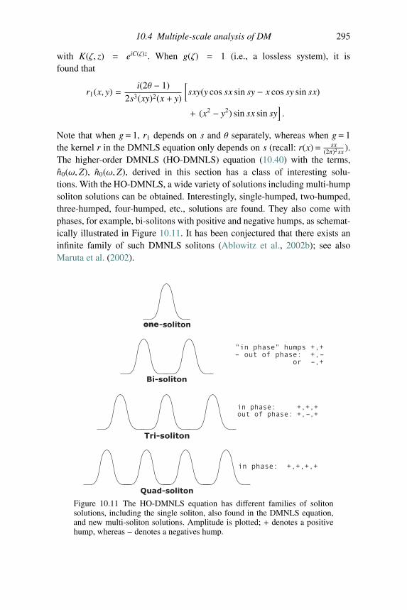
10.4 Multiple-scale analysis of DM 295
with K(ζ, z) = eiC(ζ)z. When g(ζ) = 1 (i.e., a lossless system), it isfound that
r1(x, y) =i(2θ − 1)
2s3(xy)2(x + y)
[sxy(y cos sx sin sy − x cos sy sin sx)
+ (x2 − y2) sin sx sin sy].
Note that when g= 1, r1 depends on s and θ separately, whereas when g= 1the kernel r in the DMNLS equation only depends on s (recall: r(x)= sx
(2π)2 sx ).The higher-order DMNLS (HO-DMNLS) equation (10.40) with the terms,n0(ω, Z), n0(ω, Z), derived in this section has a class of interesting solu-tions. With the HO-DMNLS, a wide variety of solutions including multi-humpsoliton solutions can be obtained. Interestingly, single-humped, two-humped,three-humped, four-humped, etc., solutions are found. They also come withphases, for example, bi-solitons with positive and negative humps, as schemat-ically illustrated in Figure 10.11. It has been conjectured that there exists aninfinite family of such DMNLS solitons (Ablowitz et al., 2002b); see alsoMaruta et al. (2002).
one
Figure 10.11 The HO-DMNLS equation has different families of solitonsolutions, including the single soliton, also found in the DMNLS equation,and new multi-soliton solutions. Amplitude is plotted; + denotes a positivehump, whereas − denotes a negatives hump.
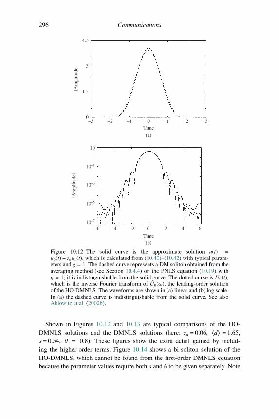
296 Communications
–3
–6 –4 –2 0 2 4 6
0
1.5
3
4.5
10
10–1
10–3
10–5
10–7
–2 –1 0Time
|Am
plitu
de|
|Am
plitu
de|
Time
(a)
(b)
1 2 3
Figure 10.12 The solid curve is the approximate solution u(t) =u0(t)+ zau1(t), which is calculated from (10.40)–(10.42) with typical param-eters and g = 1. The dashed curve represents a DM soliton obtained from theaveraging method (see Section 10.4.4) on the PNLS equation (10.19) withg = 1; it is indistinguishable from the solid curve. The dotted curve is U0(t),which is the inverse Fourier transform of U0(ω), the leading-order solutionof the HO-DMNLS. The waveforms are shown in (a) linear and (b) log scale.In (a) the dashed curve is indistinguishable from the solid curve. See alsoAblowitz et al. (2002b).
Shown in Figures 10.12 and 10.13 are typical comparisons of the HO-DMNLS solutions and the DMNLS solutions (here: za = 0.06, 〈d〉 = 1.65,s= 0.54, θ = 0.8). These figures show the extra detail gained by includ-ing the higher-order terms. Figure 10.14 shows a bi-soliton solution of theHO-DMNLS, which cannot be found from the first-order DMNLS equationbecause the parameter values require both s and θ to be given separately. Note
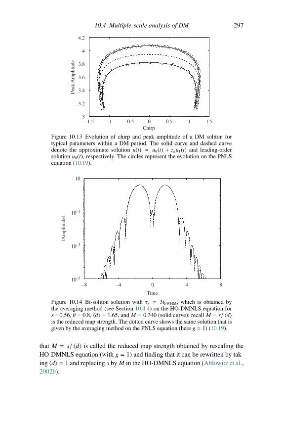
10.4 Multiple-scale analysis of DM 297
4.2
4
3.8
Peak
Am
plitu
de3.6
3.4
3.2
3–1.5 –1 –0.5 0 0.5 1 1.5
Chirp
Figure 10.13 Evolution of chirp and peak amplitude of a DM soliton fortypical parameters within a DM period. The solid curve and dashed curvedenote the approximate solution u(t) = u0(t) + zau1(t) and leading-ordersolution u0(t), respectively. The circles represent the evolution on the PNLSequation (10.19).
10
10–1
|Am
plitu
de|
10–3
10–5
–8 –4 0 4 8
Time
Figure 10.14 Bi-soliton solution with τs = 3tFWHM, which is obtained bythe averaging method (see Section 10.4.4) on the HO-DMNLS equation fors= 0.56, θ = 0.8, 〈d〉 = 1.65, and M = 0.340 (solid curve); recall M = s/ 〈d〉is the reduced map strength. The dotted curve shows the same solution that isgiven by the averaging method on the PNLS equation (here g = 1) (10.19).
that M = s/ 〈d〉 is called the reduced map strength obtained by rescaling theHO-DMNLS equation (with g = 1) and finding that it can be rewritten by tak-ing 〈d〉 = 1 and replacing s by M in the HO-DMNLS equation (Ablowitz et al.,2002b).
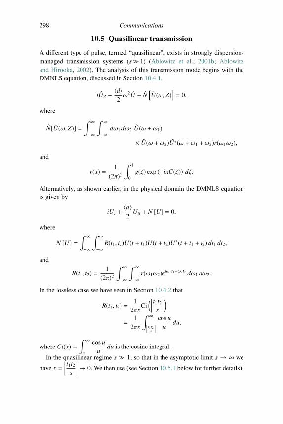
298 Communications
10.5 Quasilinear transmission
A different type of pulse, termed “quasilinear”, exists in strongly dispersion-managed transmission systems (s� 1) (Ablowitz et al., 2001b; Ablowitzand Hirooka, 2002). The analysis of this transmission mode begins with theDMNLS equation, discussed in Section 10.4.1,
iUZ − 〈d〉2 ω2U + N[U(ω, Z)
]= 0,
where
N[U(ω, Z)] =∫ ∞
−∞
∫ ∞
−∞dω1 dω2 U(ω + ω1)
× U(ω + ω2)U∗(ω + ω1 + ω2)r(ω1ω2),
and
r(x) =1
(2π)2
∫ 1
0g(ζ) exp (−ixC(ζ)) dζ.
Alternatively, as shown earlier, in the physical domain the DMNLS equationis given by
iUz +〈d〉2
Utt + N [U] = 0,
where
N [U] =∫ ∞
−∞
∫ ∞
−∞R(t1, t2)U(t + t1)U(t + t2)U∗(t + t1 + t2) dt1 dt2,
and
R(t1, t2) =1
(2π)2
∫ ∞
−∞
∫ ∞
−∞r(ω1ω2)eiω1t1+ω2t2 dω1 dω2.
In the lossless case we have seen in Section 10.4.2 that
R(t1, t2) =1
2πsCi(∣∣∣∣∣ t1t2
s
∣∣∣∣∣)=
12πs
∫ ∞∣∣∣∣ t1 t2s
∣∣∣∣cos u
udu,
where Ci(x) ≡∫ ∞
x
cos uu
du is the cosine integral.
In the quasilinear regime s � 1, so that in the asymptotic limit s → ∞ we
have x =∣∣∣∣∣ t1t2
s
∣∣∣∣∣→ 0. We then use (see Section 10.5.1 below for further details),
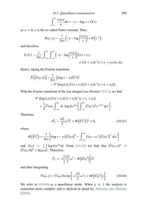
10.5 Quasilinear transmission 299∫ ∞
x
cos uu
du = −γ − log x + O(x)
as x→ 0; γ is the so-called Euler constant. Thus,
R(t1, t2) ∼ 12πs
(−γ − log
∣∣∣∣∣ t1t2s
∣∣∣∣∣) + O(s−1),
and therefore
N (U) ∼ 12πs
∫ ∞
−∞
∫ ∞
−∞
(−γ − log
∣∣∣∣∣ t1t2s
∣∣∣∣∣)U(t + t1)
× U(t + t2)U∗(t + t1 + t2) dt1 dt2.
Hence, taking the Fourier transform
N[U(ω, Z)
]∼ 1
2πs
{(log s − γ)|U |2U
− F {log |t1t2|U(t + t1)U(t + t2)U∗(t + t1 + t2)}}.
With the Fourier transform of the last integral (see Section 10.5.1), we find
F {log |t1t2|U(t + t1)U(t + t2)U∗(t + t1 + t2)}
=1π
U(ω)∫ ∞
−∞dt log |t| eiωt
[∫ ∞
−∞|U(ω′)|2e−iω′t dω′
].
Therefore
iUz − 〈d〉2 ω2U + Φ(|U |2)
U = 0, (10.43)
where
Φ(|U |2)=
12πs
[(log s − γ)
∣∣∣U(ω)∣∣∣2 − ∫ ∞
−∞f (ω − ω′) ∣∣∣U(ω′)
∣∣∣2 dω′]
and f (ω) = 1π
∫log |t| eiωtdt. From (10.43) we find that |U(ω, z)|2 =
|U(ω, 0)|2 = |u0(ω)|2. Therefore,
Uz = −i
[ 〈d〉2ω2 − Φ
(|U0|2
)]U,
and after integrating
U(ω, z) = U(ω, 0) exp
[−i〈d〉2ω2z + iΦ
(|U0|2
)z
]. (10.44)
We refer to (10.44) as a quasilinear mode. When g � 1 the analysis issomewhat more complex and is derived in detail by Ablowitz and Hirooka(2002).
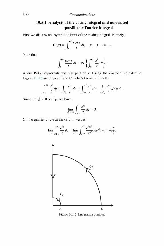
300 Communications
10.5.1 Analysis of the cosine integral and associatedquasilinear Fourier integral
First we discuss an asymptotic limit of the cosine integral. Namely,
Ci(x) =∫ ∞
x
cos tt
dt, as x→ 0 + .
Note that ∫ ∞
x
cos tt
dt = Re
{∫ ∞
x
eit
tdt
}.
where Re(x) represents the real part of x. Using the contour indicated inFigure 10.15 and appealing to Cauchy’s theorem (x > 0),∫ ∞
x
eit
tdt +
∫CR
eiz
zdz +
∫ ix
i∞eiz
zdz +
∫Cε
eiz
zdz = 0.
Since Im{z} > 0 on CR, we have
limR→∞
∫CR
eiz
zdz = 0.
On the quarter circle at the origin, we get
limε→0
∫Cε
eiz
zdz = lim
ε→0
∫ 0
π/2
eiεeiθ
εeiθiεeiθ dθ = −i
π
2.
Figure 10.15 Integration contour.
10.5 Quasilinear transmission 301
Therefore we have ∫ ∞
x
eit
tdt =
∫ i∞
ix
eiz
zdz + i
π
2
=
∫ ∞
x
e−y
ydy + i
π
2;
thus,
I ≡∫ ∞
x
cos tt
dt = �{∫ ∞
x
eit
tdt
}=
∫ ∞
x
e−y
ydy.
Now,
I =∫ ∞
x
(e−y
y− 1
y(y + 1)
)dy +
∫ ∞
x
1y(y + 1)
dy
=
∫ ∞
0
(e−y − 1
y+1
)y
dy +∫ x
0
(e−y − 1
y+1
)y
dy +∫ ∞
x
1y(y + 1)
dy.
Note that
e−y − 1y+1
y∼ e−y − (1 − y + y2 − · · · )
∼[1 − y +
y2
2− · · · − (1 − y + y2 − · · · )
]/y
∼ − y2+ · · · ,
showing the integral∫ ∞
0
e−y − 1y+1
ydy is convergent as y → 0 (the integral
clearly converges at the infinite upper limit) and it is well known that∫ ∞
0
(e−y − 1
y+1
)y
dy ≡ −γ,
where γ is the Euler constant γ � 0.57722. Also∫ x
0
(e−y − 1
y+1
)y
dy ∼x→0− x2
2+ · · ·
Similarly, ∫ ∞
x
1y(y + 1)
dy =∫ ∞
x
(1y− 1
y + 1
)dy
= log(1 + x) − log(x) ∼x→0
x − log x.
Putting this all together implies, as x→ 0+,
I ∼ −γ − log x + x + O(x2).
302 Communications
We now consider the Fourier integral
F =F{∫ ∞
−∞
∫ ∞
−∞log |t1t2|U(t + t1)U(t + t2)U∗(t + t1 + t2) dt1 dt2
}=
1(2π)3
∫ ∞
−∞e−iωt dt
∫ ∫dt1 dt2 log |t1t2|
[∫ ∞
−∞U(ω1)eiω1(t+t1) dω1
]×[∫ ∞
−∞U(ω2)eiω2(t+t2) dω2
] [∫ ∞
−∞U∗(ω3)e−iω3(t+t1+t2) dω3
].
Noting that the function is symmetric in t1, t2 and using∫
dt2 eiω2t2 e−iω3t2 =
2πδ(ω2 − ω3), we have
F =2
(2π)2
∫ ∞
−∞dt∫ ∞
−∞dt1 log |t1|∫ ∞
−∞
∫ ∞
−∞
∫ ∞
−∞dω1 dω2 dω3 ei(ω1−ω3)t1 U(ω1)U(ω2)U∗(ω3)
× δ(ω2 − ω3)ei(ω1+ω2−ω3−ω)t
=1
2π2
∫ ∞
−∞dt∫ ∞
−∞dt1 log |t1|
∫ ∞
−∞dω1dω3 U(ω1)U(ω3)U∗(ω3)
× ei(ω1−ω)tei(ω1−ω3)t1 .
Using∫ ∞−∞ dt ei(ω1−ω)t = 2πδ(ω1 − ω) implies
F =1π
∫ ∞
−∞dt1 log |t1|
∫ ∞
−∞dω3 U(ω)
∣∣∣U(ω3)∣∣∣2 ei(ω−ω3)t1 .
Or finally,
F = U(ω)∫ ∞
−∞
∣∣∣U(ω′)∣∣∣2 f (ω − ω′) dω′,
where f (x) is the generalized function,
f (x) =∫ ∞
−∞dt
log |t|π
eixt.
For calculation, it is preferable to use F in the form
F =1π
U(ω)∫ ∞
−∞dt log |t| eiωt
[∫ ∞
−∞
∣∣∣U(ω′)∣∣∣2 e−iω′t dω′
].
When a Gaussian shape is taken, |U(ω)| = αe−βω2, then the inner integral
decays rapidly as |t| → ∞.
10.6 WDM and soliton collisions 303
10.6 WDM and soliton collisions
As mentioned earlier, in a WDM system solitons are transmitted at many dif-ferent wavelengths, or frequencies; these different wavelengths are often called“channels”. Due to the dispersion in the fiber, solitons at different wavelengthstravel at different velocities. This leads to inevitable collisions between solitonsin different wavelength channels.
Considering the case of only two WDM channels, centered at the normalizedradial frequencies Ω1 and Ω2 we take two pulses u1 and u2 in channel 1 and 2respectively. The average frequency of the pulses can be calculated as
〈ω〉 = Im
{∫ ∞
−∞u∗j∂u j
∂tdt
}/Wj =
12πWj
∫ ∞
−∞ω|u j(ω)|2 dω, (10.45)
where u j(ω) is the Fourier transform of u(t), Wj =∫ ∞−∞ |uj(t)|2 dt, the energy of
pulse uj, and j ∈ {1, 2} is the channel number. The right-hand side of (10.45)is obtained by replacing u(t) by its Fourier transform.
In Section 10.2.1, we saw that the NLS equation with XPM contributions[see (10.12) and (10.13)] for channel 1 (u1) is
i∂u1
∂z+
12∂2u1
∂t2+ g(z)|u1|2u1 = −2g(z)|u2|2u1 (10.46)
and for channel 2 (u2) is
i∂u2
∂z+
12∂2u2
∂t2+ g(z)|u2|2u2 = −2g(z)|u1|2u2.
We assume the signals u1 and u2 have negligible overlap in the frequencydomain and that the FWM contribution is small. This assumption enables us toseparate the components at different frequencies in the original perturbed NLS(PNLS) equation; i.e., one considers each equation as being valid in separateregions of Fourier space.
Assuming Wj is constant, the change in average frequency can be foundfrom (10.45):
Wjddz
⟨ω j
⟩=∂
∂zIm
{∫ ∞
−∞
∂u j
∂tu∗j dt
},
= Im
⎧⎪⎨⎪⎩∫ ∞
−∞
⎛⎜⎜⎜⎜⎝∂2u j
∂t∂zu∗j +
∂u j
∂t
∂u∗j∂z
⎞⎟⎟⎟⎟⎠ dt
⎫⎪⎬⎪⎭ . (10.47)
The NLS equation for channel u1 with a perturbation F1 is
iu1z +d2
u1tt + g|u1|2u1 = F1.
304 Communications
Operating on the above equation with −iu∗1∂t and adding to the result iu1t timesthe complex conjugate of the above equation, we find
∂2u j
∂t∂zu∗j +
∂u j
∂t
∂u∗j∂z=
id2
(u∗1u1ttt − u1tu
∗1tt
)+ ig
(u∗1∂t(|u1|2u1) − |u1|2u∗1u1t
)+ i(u1tF
∗1 − u∗1F1t
).
Substituting this result into (10.47) and integrating the first two terms by parts(assuming u1 and its derivatives vanish at t = ±∞), we find
W1d 〈ω1〉
dz= Im
{∫ ∞
−∞i(F1u∗1t + F∗1u1t
)dt
}=
∫ ∞
−∞
(F1u∗1t + F∗1u1t
)dt.
If we take F1 = −2g(z)|u2|2u1 as indicated by (10.46), then
W1d 〈ω1〉
dz= 2g(z)
∫ ∞
−∞|u1|2∂t |u2|2 dt,
or more generally
d⟨ω j
⟩dz
=2g(z)Wj
∫ ∞
−∞|uj|2∂t |u3− j|2 dt, j = 1, 2. (10.48)
The frequency shift is found by integrating (10.48). Similarly, the timingshift may be found from the definition of the average position in time,
⟨t j
⟩,
j = 1, 2:
Wj
⟨t j
⟩=
∫ ∞
−∞t |uj|2 dt.
Thus, again assuming Wj is constant,
W1ddz〈t1〉 = ∂
∂z
(∫ ∞
−∞t |u1|2 dt
)=
∫ ∞
−∞t
(u∗1∂u1
∂z+∂u∗1∂z
u1
)dt
=
∫ ∞
−∞t
{u∗1
[id2
u1tt + ig(z)u21u∗1 − iF1
]}dt
+
∫ ∞
−∞t
{u1
[− id
2u∗1tt − ig(z)
(u∗1)2 u1 + iF∗1
]}dt
= − id2
∫ ∞
−∞
(u∗1u1t − u1u∗1t
)dt − i
∫ ∞
−∞t(u∗1F1 − u1F∗1
)dt.
10.6 WDM and soliton collisions 305
Recalling
Wj
⟨ω j
⟩= Im
{∫ ∞
−∞
∂u j
∂tu∗j dt
}=
12i
∫ ∞
−∞
⎛⎜⎜⎜⎜⎝∂u j
∂tu∗j −
∂u∗j∂t
u j
⎞⎟⎟⎟⎟⎠ dt,
we can write
W1ddz〈t1〉 = d(z)W1 〈ω1〉 − i
∫ ∞
−∞t(u∗1F1 − u1F∗1
)dt.
Using F1 = −2g(z) |u2|2 u1, the integral∫ ∞−∞ t
(u∗1F1 − u1F∗1
)dt = 0 and we
obtainddz〈t1〉 = d(z) 〈ω1〉 . (10.49)
The timing shift may be obtained by integrating (10.49) with respect to z.In the context of RZ (return to zero) soliton or quasilinear communications
systems it is useful to define the residual frequency shift as the relative fre-quency shift of the pulse at the end of the communications system. Usinga system starting at z = 0 and of length L, with this definition the residualfrequency shift of a pulse in channel j is given by
ΔΩ( j)res =
⟨ω j
⟩(L) − 〈ω〉 (0) =
∫ L
0
d⟨ω j
⟩dz
dz.
We are also interested in the relative timing shift at the end of the collisionprocess. The total timing shift, (10.49), yields
ddz
⟨t j
⟩(z) = d(z)
[⟨ω j
⟩(z) −
⟨ω j
⟩(0)]+ d(z)
⟨ω j
⟩(0)
= d(z)∫ z
0
d⟨ω j
⟩dz
dz + d(z)⟨ω j
⟩(0).
Defining d(z) =∫ z
0d(z′) dz′, and integrating the above equation from z = 0 to
z = L, ⟨t j
⟩(L) −
⟨t j
⟩(0) =
∫ L
0d(z)
∫ z
0
d 〈ω〉 j
dz′dz′ dz + d(L)
⟨ω j
⟩(0).
Note that⟨t j
⟩(0) + d(L)
⟨ω j
⟩(0) is invariant. We can also define the relative
timing shift as
Δt j(L) ≡⟨t j
⟩(L) −
⟨t j
⟩(0) − d(L)
⟨ω j
⟩(0) =
∫ L
0d(z)
∫ z
0
d 〈ω〉 j
dz′dz′ dz.
306 Communications
This can now be simplified by changing the order of integration:
Δt j(L) =∫ L
0d(z)
∫ z
0
d 〈ω〉 j
dz′dz′ dz (10.50)
=
∫ L
0
d 〈ω〉 j
dz′
∫ L
z′D(z) dz dz′
=
∫ L
0
d 〈ω〉 j
dz′[d(L) − d(z′)
]dz′
= d(L)∫ L
0
d 〈ω〉 j
dz′dz′ −
∫ L
0
d 〈ω〉 j
dz′d(z′) dz′
= d(L)ΔΩ( j)res −
∫ L
0
d 〈ω〉 j
dz′d(z′) dz′.
Thus, the relative timing shift can be written as the difference of two terms:
Δt j(L) = d(L)ΔΩ( j)res − Δt( j)
res,
where the so-called residual timing shift is
Δt( j)res ≡
∫ L
0
d 〈ω〉 j
dzd(z) dz.
10.7 Classical soliton frequency and timing shifts
In this section we obtain the frequency and time shift for classical solitons; seealso Mollenauer et al. (1991). Using the classical soliton shape
uj = η j sech[η j(t −Ω jz)] eiΩ j t+i(η2
j−Ω2)/2+iφ j ,
we substitute this into (10.48) to find
d⟨ω j
⟩dz
=g(z)η j
∫ ∞
−∞ddt
{η2
3− j sech2[η3− j
(t −Ω3− j(z − z0)
)]}× η2
j sech2[η j
(t −Ω j(z − z0)
)]dt.
Note that the classical soliton frequency is⟨ω j
⟩= Ω j. For |Ω j| � 1 we take
Ω j approximately being a constant within the integral. Then we can transformthe derivative in t to one in z:
dΩ j
dz=
g(z)η23− jη j
Ω3− j
∫ ∞
−∞ddz
{sech2
[η3− j
×(t −Ω3− j(z − z0)
)]}sech2
[η j
(t −Ω j(z − z0)
)]dt.
10.7 Classical soliton frequency and timing shifts 307
To simplify this integral we assume that the solitons are both of equal energy(amplitude) with η1 = η2 = η and we take a frame of reference whereΩ1 =−Ω2 = Ω. For an arbitrary frame of reference we may define Ω, withoutloss of generality, as half the frequency separation:
Ω ≡ 12
(Ω1 −Ω2).
With this substitution the average frequency change can be simplified to
dΩdz=
g(z)η3
2Ωddz
∫ ∞
−∞sech2 [η (t −Ω(z − z0))
]× sech2 [η (t + Ω(z − z0))
]dt.
Performing the integration in time analytically, we obtain an expression for thefrequency shift, ΔΩ = Ω(z) − Ω(−∞) (we take the “initial” frequency to begiven at large negative values of z that is taken to be −∞):
ΔΩ(z) =2η2
Ω
×∫ z
−∞g(z′)
ddz′
2ηΩ(z′ − z0) cosh 2ηΩ(z′ − z0) − sinh 2ηΩ(z′ − z0)
sinh3 2ηΩ(z′ − z0)dz′.
We can similarly calculate the timing shift. First we assume a constant dis-persion of d(z) = 1. Then we can calculate the residual timing shift byusing (10.50) (and integration by parts)
Δt(z) =∫ z
−∞ΔΩ(z′) dz′.
From these equations we can calculate the frequency and timing shifts for aclassical soliton collision. A typical collision is shown in Figure 10.16, wherethe propagating path is shown explicitly; the soliton is injected into the systemat z = 0 at a time position of t0 for u1 and −t0 for u2; they meet and collidewith a collision center of z0 and propagate onward until the end of the systemat z = L. The initial location of the solitons, t0, is related to the center ofcollision by
t0 = ΩDz0.
The frequency shift is shown in Figure 10.17a over the distance of the col-lision relative to its center, z0. The frequency shift is maximal at the center ofthe collision and returns to zero after the collision for the lossless case (g = 1).For the “lossy” case, g � 1 (i.e., with damping and amplification included
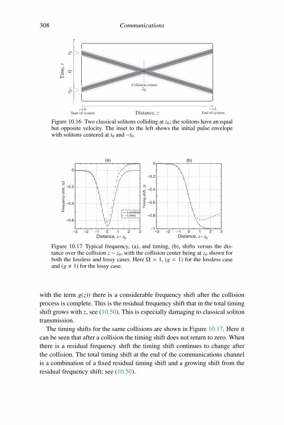
308 Communications
Distance, z
z0
z = 0 z = LStart of system
Collision center,
End of system
Tim
e, t
0t0
–t0
Figure 10.16 Two classical solitons colliding at z0; the solitons have an equalbut opposite velocity. The inset to the left shows the initial pulse envelopewith solitons centered at t0 and −t0.
–3 –2 –1 0 1 2 3Distance, z – z0 Distance, z – z0
–0.6
–0.4
–0.2
0
Freq
uenc
y sh
ift, Δ
Ω
LosslessLossy
–3 –2 –1 0 1 2 3–1
–0.8
–0.6
–0.4
–0.2
0
Tim
ing
shift
, Δt
(a) (b)
Figure 10.17 Typical frequency, (a), and timing, (b), shifts versus the dis-tance over the collision z − z0, with the collision center being at z0 shown forboth the lossless and lossy cases. Here Ω = 1, (g = 1) for the lossless caseand (g � 1) for the lossy case.
with the term g(z)) there is a considerable frequency shift after the collisionprocess is complete. This is the residual frequency shift that in the total timingshift grows with z, see (10.50). This is especially damaging to classical solitontransmission.
The timing shifts for the same collisions are shown in Figure 10.17. Here itcan be seen that after a collision the timing shift does not return to zero. Whenthere is a residual frequency shift the timing shift continues to change afterthe collision. The total timing shift at the end of the communications channelis a combination of a fixed residual timing shift and a growing shift from theresidual frequency shift; see (10.50).
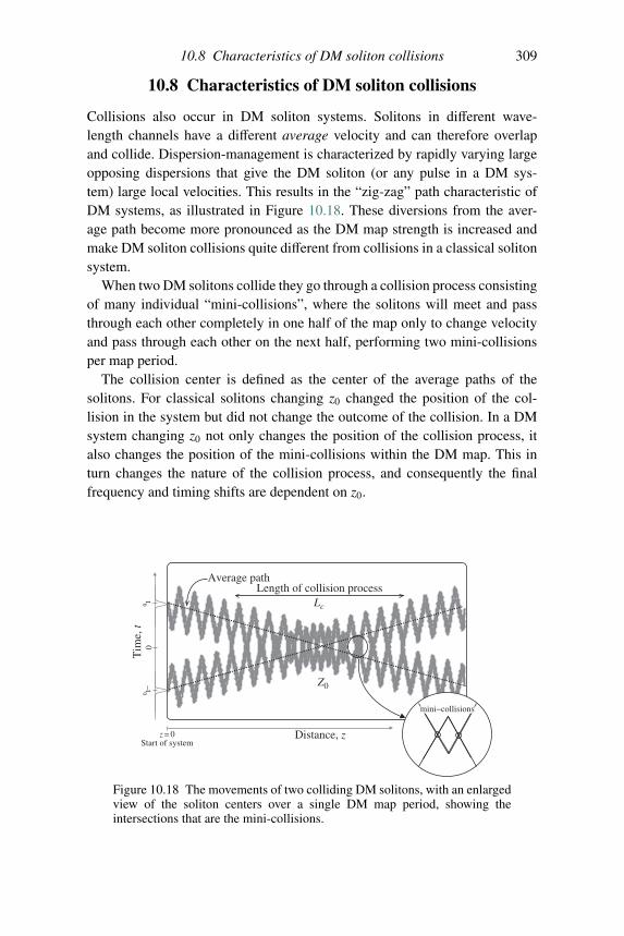
10.8 Characteristics of DM soliton collisions 309
10.8 Characteristics of DM soliton collisions
Collisions also occur in DM soliton systems. Solitons in different wave-length channels have a different average velocity and can therefore overlapand collide. Dispersion-management is characterized by rapidly varying largeopposing dispersions that give the DM soliton (or any pulse in a DM sys-tem) large local velocities. This results in the “zig-zag” path characteristic ofDM systems, as illustrated in Figure 10.18. These diversions from the aver-age path become more pronounced as the DM map strength is increased andmake DM soliton collisions quite different from collisions in a classical solitonsystem.
When two DM solitons collide they go through a collision process consistingof many individual “mini-collisions”, where the solitons will meet and passthrough each other completely in one half of the map only to change velocityand pass through each other on the next half, performing two mini-collisionsper map period.
The collision center is defined as the center of the average paths of thesolitons. For classical solitons changing z0 changed the position of the col-lision in the system but did not change the outcome of the collision. In a DMsystem changing z0 not only changes the position of the collision process, italso changes the position of the mini-collisions within the DM map. This inturn changes the nature of the collision process, and consequently the finalfrequency and timing shifts are dependent on z0.
Average path
Z0
Lc
Length of collision process
Distance, z
Tim
e, t
0t0
–t0
z = 0Start of system
mini−collisions
Figure 10.18 The movements of two colliding DM solitons, with an enlargedview of the soliton centers over a single DM map period, showing theintersections that are the mini-collisions.
310 Communications
As with classical soliton collisions the initial time displacement at the startof the channel can be calculated from the collision center, defined as
t0 = Ω j 〈d〉 z0,
with j ∈ {1, 2} indicating one of the two frequency channels.The center of a DM soliton satisfies t(n)
c − Ω jd(z) = 0 for t(n)c and z, with n ∈
{1, 2} indicating one of the two frequency channels. An approximate analyticalformula for a DM soliton is given in the next section; see (10.51). Using thiswe can find the locations of the mini-collisions, those values of z at which thecenters of both solitons are coincident, namely t(1)
c = t(2)c :
Ω1d(z) = Ω2d(z)
so that
d(z) = 0.
Therefore mini-collision locations are found from the solution of d(z) =〈d〉 (z − z0) + C(z) = 0, and are not influenced by the average frequencies ofeither soliton. The range of the chirp, C(z), is limited; it periodically oscillatesbetween min{C(z)} and max{C(z)}. As a consequence d(z) = 0 only has solu-tions over a limited domain, which corresponds to the extent of the collisionprocess. When 〈d〉 (z − z0) is larger or smaller than the range of C(z), there areno mini-collisions, and we can therefore estimate the extent of the collision as
−max{C(z)} < 〈d〉 (z − z0) < −min{C(z)}z0 − s/ 〈d〉 < z < z0 + s/ 〈d〉 ,
where max{C(z)} = −min{C(z)} = s = θΔ1/2. The length of the collisionLC = 2s/ 〈d〉 is the difference of the upper and lower collision limits, and wenotice that the larger the map strength the longer is the DM soliton’s collisionprocess.
10.9 DM soliton frequency and timing shifts
We have seen in Section 10.4 that u = Ue−iCω2/2. If we approximate U byU = αe−βω2/2, then a DM soliton can be approximated in physical space by
u1(z, t) =α√
2π(β + iC(z))exp
{− [t −Ω1d(z)]2
2[β + iC(z)]
}× exp
{ i2
[λ2z + 2Ω1t −Ω2
1d(z)]}, (10.51)
10.9 DM soliton frequency and timing shifts 311
where d(z) − 〈d〉 z0 =
∫ z
z0
d(z′) dz′ = (z − z0) 〈d〉 +C(z). Substituting the above
DM soliton representation for u1 and u2 into (10.48) we get
d⟨ω j
⟩dz
= − g(z)α jα3− jβ3− j
2π[β2
j +C2(z)]1/2 [
β23− j +C2(z)
]5/2×∫ ∞
−∞[t −Ω3− jd(z)] exp
⎧⎪⎪⎪⎨⎪⎪⎪⎩−β j[t −Ω jd(z)]2
2[β2
j +C2(z)] − β3− j[t −Ω3− jd(z)]2
2[β2
3− j +C2(z)]⎫⎪⎪⎪⎬⎪⎪⎪⎭ dt
for j = 1, 2. We further assume that the solitons in both channels have thesame shape; that is, α1 = α2 and β1 = β2. With this assumption and noting⟨ω j
⟩= Ω j, we obtain an analytic formula for DM soliton collision-induced
frequency shifts,
dΩ1
dz= (A/2)(Ω1 −Ω2)
d(z)g(z)B3(z)
exp
⎛⎜⎜⎜⎜⎜⎝−(β/2)
[d(z)B(z)
(Ω1 −Ω2)
]2⎞⎟⎟⎟⎟⎟⎠ , (10.52)
where dΩ1/dz = −dΩ2/dz and in order to simplify this and equations thatfollow, we use the following definitions:
A =4Wβ3/2
√2π
,
B2(z) = β2 +C2(z/za).
We remark that in the case of quasilinear pulses the only difference turnsout to be the definition of B(z); for quasilinear pulses, we use B2(z) =β2 + (d)2(z). Because the two-channel system is symmetric, we can, with-out loss of generality, define Ω = (Ω1 − Ω2)/2. The residual frequencyshift, ΔΩ(z) = Ω(z) − Ω(−∞), is obtained by integration of (10.52). Assum-ing Ω(z) is a slowly varying function (i.e., |dΩ/dz| � 1) which must bethe case for the validity of the perturbation method (and is verified a pos-teriori), we can treat Ω on the right-hand side of (10.52) as a constant,obtaining
ΔΩ(z) = AΩ∫ z
0
g(z)d(z)B3(z)
exp
⎡⎢⎢⎢⎢⎢⎣−2β
(d(z)B(z)Ω
)2⎤⎥⎥⎥⎥⎥⎦ dz. (10.53)
We can also obtain the timing shift from (10.50):
Δt(L) = d(L)ΔΩ(L) −∫ L
0
d 〈ω〉dz′
d(z′) dz′. (10.54)
312 Communications
Ablowitz et al. (2002a, 2003b), Docherty (2003), and Ahrens (2006) thedetails of various types of collisions describe. There it is shown that directnumerical computation of the NLS equation agrees with numerical evalu-ation of (10.53) and (10.54), which also agree with asymptotic evaluationof (10.53) and (10.54) by employing the asymptotic analysis of integrals usinga modification of the Laplace method.
11Mode-locked lasers
In the previous chapter we have seen that both constant dispersion anddispersion-managed solitons are important pulses in the study of long-distancetransmission/communications. It is noteworthy that experiments reveal thatsolitons or localized pulses are also present in mode-locked (ML) lasers.Femtosecond solid-state lasers, such as those based on the Ti:sapphire (Ti:S)gain medium, and fiber ring lasers have received considerable attention inthe field of ultra-fast science. In the past decade, following the discoveryof mode-locking, the improved performance of these lasers has led to theirwidespread use, cf. Cundiff et al. (2008). In most cases interest in ultra-shortpulse mode-locking has been in the net anomalous dispersive regime. Butmode-locking has also been demonstrated in fiber lasers operating in the nor-mal regime. Mode-locking operation has been achieved with relatively largepulse energies (Ilday et al., 2004b,a; Chong et al., 2008b).
In our investigations we have employed a distributive model, termed thepower-energy saturation (PES) equation (cf. Ablowitz et al., 2008; Ablowitzand Horikis, 2008, 2009b; Ablowitz et al., 2009c). This model goes beyondthe well-known master laser equation, cf. Haus (1975, 2000), in that it con-tains saturable power (intensity) terms; i.e., terms that saturate due to large fieldamplitudes. This equation has localized pulses that propagate and mode-lockin both an anomalous and a normally dispersive laser for both in the constantas well as dispersion-managed system. This is consistent with recent experi-mental observations (Ilday et al., 2004b; Chong et al., 2008a). We also notethat it has been shown that dispersion-managed models with saturable power(intensity) energy saturation terms are in good agreement with experimentalresults in Ti:sapphire lasers (Sanders et al., 2009b). Pulse formation in an ultra-short pulse laser is typically dominated by the interplay between dispersion andnonlinearity. Suitable gain media and an effective saturable absorber are essen-tial for initiating the mode-locking operation from intra-cavity background
313
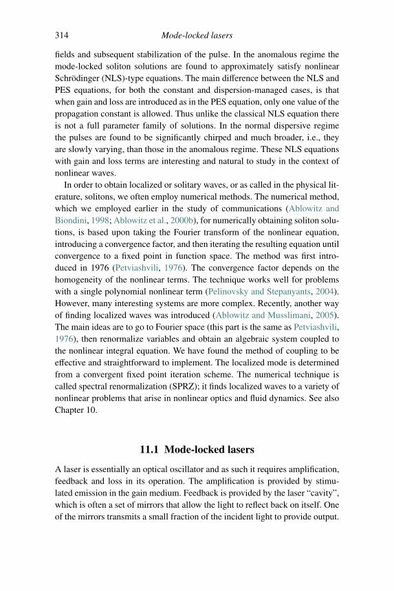
314 Mode-locked lasers
fields and subsequent stabilization of the pulse. In the anomalous regime themode-locked soliton solutions are found to approximately satisfy nonlinearSchrodinger (NLS)-type equations. The main difference between the NLS andPES equations, for both the constant and dispersion-managed cases, is thatwhen gain and loss are introduced as in the PES equation, only one value of thepropagation constant is allowed. Thus unlike the classical NLS equation thereis not a full parameter family of solutions. In the normal dispersive regimethe pulses are found to be significantly chirped and much broader, i.e., theyare slowly varying, than those in the anomalous regime. These NLS equationswith gain and loss terms are interesting and natural to study in the context ofnonlinear waves.
In order to obtain localized or solitary waves, or as called in the physical lit-erature, solitons, we often employ numerical methods. The numerical method,which we employed earlier in the study of communications (Ablowitz andBiondini, 1998; Ablowitz et al., 2000b), for numerically obtaining soliton solu-tions, is based upon taking the Fourier transform of the nonlinear equation,introducing a convergence factor, and then iterating the resulting equation untilconvergence to a fixed point in function space. The method was first intro-duced in 1976 (Petviashvili, 1976). The convergence factor depends on thehomogeneity of the nonlinear terms. The technique works well for problemswith a single polynomial nonlinear term (Pelinovsky and Stepanyants, 2004).However, many interesting systems are more complex. Recently, another wayof finding localized waves was introduced (Ablowitz and Musslimani, 2005).The main ideas are to go to Fourier space (this part is the same as Petviashvili,1976), then renormalize variables and obtain an algebraic system coupled tothe nonlinear integral equation. We have found the method of coupling to beeffective and straightforward to implement. The localized mode is determinedfrom a convergent fixed point iteration scheme. The numerical technique iscalled spectral renormalization (SPRZ); it finds localized waves to a variety ofnonlinear problems that arise in nonlinear optics and fluid dynamics. See alsoChapter 10.
11.1 Mode-locked lasers
A laser is essentially an optical oscillator and as such it requires amplification,feedback and loss in its operation. The amplification is provided by stimu-lated emission in the gain medium. Feedback is provided by the laser “cavity”,which is often a set of mirrors that allow the light to reflect back on itself. Oneof the mirrors transmits a small fraction of the incident light to provide output.

11.1 Mode-locked lasers 315
The loss that counteracts gain is due to a variety of factors such as a field cutoffor polarization effects, etc.
A mode-locked pulse refers to the description of how ultra-short pulses aregenerated by a laser. The formation of a mode means that the electromagneticfield is essentially unchanged after one round trip in the laser. This implies thatlasing occurs for those frequencies for which the cavity length is an integernumber of wavelengths. If multiple modes lase at the same time, then a shortpulse can be formed if the modes are also phase-locked; we say the laser ismode-locked, cf. Cundiff (2005). In terms of the mathematics of nonlinearwaves, mode-locking usually relates to specific pulse solutions admitted bythe underlying nonlinear equations.
A distinguishing feature of such a laser is the presence of an element inthe cavity that causes it to mode-lock. This can be an active or a passiveelement. Passive mode-locking has produced shorter pulses and has a saturableabsorber, i.e., one where the absorption saturates. In this case, higher intensityis less attenuated than a lower intensity.
An advantage of Ti:s lasers is their large-gain bandwidth, which is necessaryfor supporting ultra-short pulses (it is useful to think of this as the Fourierrelationship). The gain band is typically quoted as extending from 700 to1000 nm, although lasing can be achieved well beyond 1000 nm. The Ti:scrystal provides the essential mode-locking mechanism in these lasers. Thisis due to a strong cubic nonlinear index of refraction (the Kerr effect), whichis manifested as an increase of the index of refraction as the optical intensityincreases. Together with a correctly positioned effective aperture, the nonlin-ear Kerr-lens can act as a saturable absorber, i.e., high intensities are focusedand hence transmit fully through the aperture while low intensities experi-ence losses. Since short pulses produce higher peak powers, they experiencea lower loss that also favors a mode-locked operation. This mode-lockingmechanism has the advantage of being essentially instantaneous. However,it has the disadvantage of often being not self-starting; typically it requiresa critical misalignment from optimum continuous wave operation. Ti:s laserscan produce pulses on the order of a few femtoseconds. An application ofinterest is producing a very long string of equally spaced mode-locked pulses:this has the potential to be used as an “optical clock” where each tick of theclock corresponds to a pulse, cf. Cundiff (2005). A schematic diagram of atypical Ti:s laser system is given in Figure 11.1 with typical units: pulsewidth:τ = 10 fs = 10−14 s and repetition time: Tr = 10 ns = 1010 s or repetition fre-quency fr = 1
Tr = 100 MHz. In this setup the prism pair is used to compensatefor the net normal dispersion of the Ti:s crystal. In the crystal we have strongnonlinear effects, but in the prism the nonlinearity is very weak. So we assume
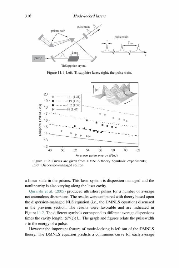
316 Mode-locked lasers
pulse trainprism pair
pump
2 mm
Ti:Sapphire crystal
Trep
t
τpulse train
Figure 11.1 Left: Ti:sapphire laser; right: the pulse train.
−−−−
Figure 11.2 Curves are given from DMNLS theory. Symbols: experiments;inset: Dispersion-managed soliton.
a linear state in the prisms. This laser system is dispersion-managed and thenonlinearity is also varying along the laser cavity.
Quraishi et al. (2005) produced ultrashort pulses for a number of averagenet anomalous dispersions. The results were compared with theory based uponthe dispersion-managed NLS equation (i.e., the DMNLS equation) discussedin the previous section. The results were favorable and are indicated inFigure 11.2. The different symbols correspond to different average dispersionstimes the cavity length: 〈k′′(z)〉 lm. The graph and figures relate the pulsewidthτ to the energy of a pulse.
However the important feature of mode-locking is left out of the DMNLStheory. The DMNLS equation predicts a continuous curve for each average
11.2 Power-energy-saturation equation 317
dispersion value. But the experiments indicate that there is not a continuouscurve, rather for each value of energy there is one mode-locked configuration.This is discussed next as part of the mathematical model.
11.2 Power-energy-saturation equation
The distributed model that we use to describe the propagation of pulses in alaser cavity is given in dimensionless form by
iuz +d(z)
2utt + n(z)|u|2u =
ig1 + E/E0
u +iτ
1 + E/E0utt − il
1 + P/P0u, (11.1)
where d(z), n(z) are the dispersion and coefficient of nonlinearity, each ofwhich vary rapidly in z, E(z) =
∫ ∞−∞ |u|2 dt is the pulse energy, E0 is related
to the saturation energy, P(z, t) = |u|2 is the instantaneous pulse power, P0
is related to the saturation power, and the parameters g, τ, l, are all positive,real constants. The first term on the right-hand side represents saturable gain,the second is spectral filtering and the third saturable loss that reflects the fastsaturable absorber: l
1+P/P0.
Notice that gain and filtering are saturated with energy while loss is saturatedwith power. The gain and filtering mechanisms are related to the energy of thepulse while the loss is related to the power (intensity) of the pulse. Saturationterms can be expected to prevent the pulse from reaching a singular state; i.e.,“infinite” energy or a blow-up in amplitude. Indeed, if blow-up were to occurthat would suggest that both the amplitude and the energy of the pulse wouldbecome large, which in turn, make the perturbing effects small thus reducingthe equation to the unperturbed NLS, which admits a stable, finite solution.
We refer to (11.1) as the power-energy-saturation equation or simply thePES equation. The right-hand side of (11.2) is what we will refer to as theperturbing contribution; it is denoted hereafter by R[u].
The PES model reflects many developments over the years. In order tomodel the effects of nonlinearity, dispersion, bandwidth limited gain, energysaturation and intensity discrimination in a laser cavity the so-called mas-ter equation was introduced, cf. Haus et al. (1992); Haus (2000). The masterequation is a generalization of the classical NLS equation, modified to containgain, filtering and loss terms; the normalized master equation, with dispersionmanagement included is given below.
iuz +d(z)
2utt + n(z)|u|2u =
ig1 + E/E0
u +iτ
1 + E/E0utt − i(l − β|u|2)u.
318 Mode-locked lasers
The master equation is obtained from the PES model by Taylor expanding thepower saturation term and putting β = l/P0. As with the PES model, gain andfiltering are saturated by energy (i.e., the time integral of the pulse power), butin the master equation the loss is converted into a linear and a cubic nonlin-ear term. For certain values of the parameters this equation exhibits a rangeof phenomena including: mode-locking evolution; pulses that disperse intoradiation; some that evolve to a non-localized quasiperiodic state; and somewhose amplitude grows rapidly (Kapitula et al., 2002). In the latter case, ifthe nonlinear gain is too high, the linear attenuation terms are unable to pre-vent the pulse from blowing up; i.e., the master mode-locking model breaksdown (Kutz, 2006). However, unlike what is observed in experiments, thereis only a small window of parameter space that allows for the generation ofstable mode-locked pulses. In particular, the model is highly sensitive to thenonlinear loss/gain parameter.
We have shown that the PES model yields mode-locking for wide rangesof the parameters (cf. Ablowitz et al., 2008; Ablowitz and Horikis, 2008,2009b; Ablowitz et al., 2009c). As mentioned above, this model is a dis-tributed equation. There are also interesting lumped models that have beenstudied (cf. Ilday et al., 2004b,a; Chong et al., 2008b); e.g., in some laser mod-els, loss is introduced in the form of fast saturable power absorbers that areplaced periodically. It has been found (Ablowitz and Horikis, 2009a), how-ever, that all features are essentially the same in both lumped and distributivemodels thus indicating that distributive models are very good descriptions ofmodes in mode-locked lasers. Lumped models reflect sharp changes in theparameters/coefficients due to corresponding elements in the system; mathe-matically these models are often dealt with by Dirac delta function transitions(see also Chapter 10). Mathematically it is also more convenient to workwith distributed models. We note that Haus (1975) derived models of fastsaturable absorbers in two-level media that are similar to the ones we arestudying here. However in order to obtain analytical results, Haus Taylor-expanded and therefore obtained the cubic nonlinear model of a fast saturableabsorber.
We also mention that to overcome the sensitivity inherent in the mas-ter equation, other types of terms, such as quintic terms, can be added tothe master equation in order to stabilize the solutions. This increases theparameter range for mode-locking somewhat (instabilities may still occur);but it also adds another parameter to the model. Cubic and quintic nonlinearmodels are based on Ginzburg–Landau-type (GL) equations (cf. Akhmedievand Ankiewicz, 1997). In fact, if the pulse energy is taken to be con-stant the master equation reduces to a GL-type system. In general, GL-type
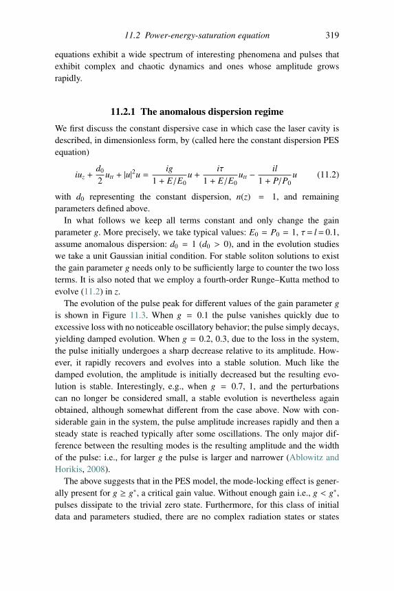
11.2 Power-energy-saturation equation 319
equations exhibit a wide spectrum of interesting phenomena and pulses thatexhibit complex and chaotic dynamics and ones whose amplitude growsrapidly.
11.2.1 The anomalous dispersion regime
We first discuss the constant dispersive case in which case the laser cavity isdescribed, in dimensionless form, by (called here the constant dispersion PESequation)
iuz +d0
2utt + |u|2u =
ig1 + E/E0
u +iτ
1 + E/E0utt − il
1 + P/P0u (11.2)
with d0 representing the constant dispersion, n(z) = 1, and remainingparameters defined above.
In what follows we keep all terms constant and only change the gainparameter g. More precisely, we take typical values: E0 = P0 = 1, τ= l= 0.1,assume anomalous dispersion: d0 = 1 (d0 > 0), and in the evolution studieswe take a unit Gaussian initial condition. For stable soliton solutions to existthe gain parameter g needs only to be sufficiently large to counter the two lossterms. It is also noted that we employ a fourth-order Runge–Kutta method toevolve (11.2) in z.
The evolution of the pulse peak for different values of the gain parameter gis shown in Figure 11.3. When g = 0.1 the pulse vanishes quickly due toexcessive loss with no noticeable oscillatory behavior; the pulse simply decays,yielding damped evolution. When g = 0.2, 0.3, due to the loss in the system,the pulse initially undergoes a sharp decrease relative to its amplitude. How-ever, it rapidly recovers and evolves into a stable solution. Much like thedamped evolution, the amplitude is initially decreased but the resulting evo-lution is stable. Interestingly, e.g., when g = 0.7, 1, and the perturbationscan no longer be considered small, a stable evolution is nevertheless againobtained, although somewhat different from the case above. Now with con-siderable gain in the system, the pulse amplitude increases rapidly and then asteady state is reached typically after some oscillations. The only major dif-ference between the resulting modes is the resulting amplitude and the widthof the pulse: i.e., for larger g the pulse is larger and narrower (Ablowitz andHorikis, 2008).
The above suggests that in the PES model, the mode-locking effect is gener-ally present for g ≥ g∗, a critical gain value. Without enough gain i.e., g < g∗,pulses dissipate to the trivial zero state. Furthermore, for this class of initialdata and parameters studied, there are no complex radiation states or states
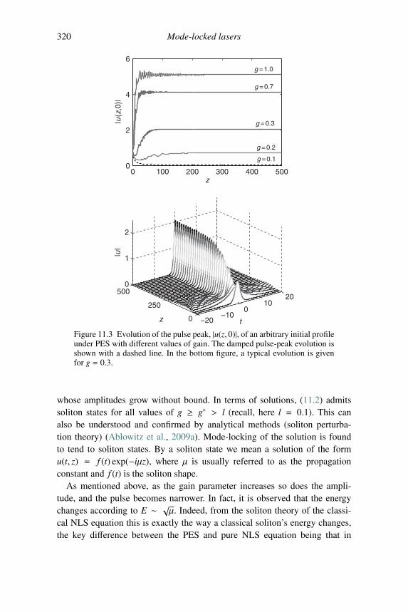
320 Mode-locked lasers
0 100 200 300 400 5000
2
4
6
z
|u(z
,0)|
g = 0.7
g = 0.3
g = 1.0
g = 0.2
g = 0.1
−20−10
010
20
0
250
5000
1
2
tz
|u|
Figure 11.3 Evolution of the pulse peak, |u(z, 0)|, of an arbitrary initial profileunder PES with different values of gain. The damped pulse-peak evolution isshown with a dashed line. In the bottom figure, a typical evolution is givenfor g = 0.3.
whose amplitudes grow without bound. In terms of solutions, (11.2) admitssoliton states for all values of g ≥ g∗ > l (recall, here l = 0.1). This canalso be understood and confirmed by analytical methods (soliton perturba-tion theory) (Ablowitz et al., 2009a). Mode-locking of the solution is foundto tend to soliton states. By a soliton state we mean a solution of the formu(t, z) = f (t) exp(−iμz), where μ is usually referred to as the propagationconstant and f (t) is the soliton shape.
As mentioned above, as the gain parameter increases so does the ampli-tude, and the pulse becomes narrower. In fact, it is observed that the energychanges according to E ∼ √μ. Indeed, from the soliton theory of the classi-cal NLS equation this is exactly the way a classical soliton’s energy changes,the key difference between the PES and pure NLS equation being that in
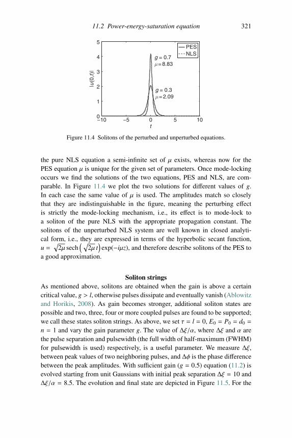
11.2 Power-energy-saturation equation 321
−10 −5 0 5 100
1
2
3
4
5
t
|u(0
,t)|
PESNLS
g = 0.7μ = 8.83
g = 0.3μ = 2.09
Figure 11.4 Solitons of the perturbed and unperturbed equations.
the pure NLS equation a semi-infinite set of μ exists, whereas now for thePES equation μ is unique for the given set of parameters. Once mode-lockingoccurs we find the solutions of the two equations, PES and NLS, are com-parable. In Figure 11.4 we plot the two solutions for different values of g.In each case the same value of μ is used. The amplitudes match so closelythat they are indistinguishable in the figure, meaning the perturbing effectis strictly the mode-locking mechanism, i.e., its effect is to mode-lock toa soliton of the pure NLS with the appropriate propagation constant. Thesolitons of the unperturbed NLS system are well known in closed analyti-cal form, i.e., they are expressed in terms of the hyperbolic secant function,u =
√2μ sech
( √2μ t)
exp(−iμz), and therefore describe solitons of the PES toa good approximation.
Soliton stringsAs mentioned above, solitons are obtained when the gain is above a certaincritical value, g > l, otherwise pulses dissipate and eventually vanish (Ablowitzand Horikis, 2008). As gain becomes stronger, additional soliton states arepossible and two, three, four or more coupled pulses are found to be supported;we call these states soliton strings. As above, we set τ = l = 0, E0 = P0 = d0 =
n = 1 and vary the gain parameter g. The value of Δξ/α, where Δξ and α arethe pulse separation and pulsewidth (the full width of half-maximum (FWHM)for pulsewidth is used) respectively, is a useful parameter. We measure Δξ,between peak values of two neighboring pulses, and Δφ is the phase differencebetween the peak amplitudes. With sufficient gain (g = 0.5) equation (11.2) isevolved starting from unit Gaussians with initial peak separation Δξ = 10 andΔξ/α = 8.5. The evolution and final state are depicted in Figure 11.5. For the
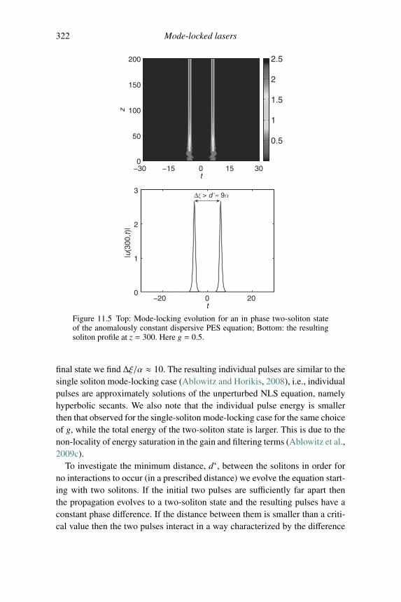
322 Mode-locked lasers
t
z
−15 0 15 30−30
50
100
150
200
0
0.5
1
1.5
2
2.5
−20 0 200
1
2
3
t
|u(3
00,t
)|
Δξ > d ∗≈ 9α
Figure 11.5 Top: Mode-locking evolution for an in phase two-soliton stateof the anomalously constant dispersive PES equation; Bottom: the resultingsoliton profile at z = 300. Here g = 0.5.
final state we find Δξ/α ≈ 10. The resulting individual pulses are similar to thesingle soliton mode-locking case (Ablowitz and Horikis, 2008), i.e., individualpulses are approximately solutions of the unperturbed NLS equation, namelyhyperbolic secants. We also note that the individual pulse energy is smallerthen that observed for the single-soliton mode-locking case for the same choiceof g, while the total energy of the two-soliton state is larger. This is due to thenon-locality of energy saturation in the gain and filtering terms (Ablowitz et al.,2009c).
To investigate the minimum distance, d∗, between the solitons in order forno interactions to occur (in a prescribed distance) we evolve the equation start-ing with two solitons. If the initial two pulses are sufficiently far apart thenthe propagation evolves to a two-soliton state and the resulting pulses have aconstant phase difference. If the distance between them is smaller than a criti-cal value then the two pulses interact in a way characterized by the difference
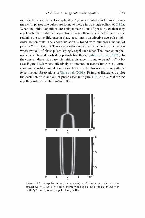
11.2 Power-energy-saturation equation 323
in phase between the peaks amplitudes: Δφ. When initial conditions are sym-metric (in phase) two pulses are found to merge into a single soliton of (11.2).When the initial conditions are antisymmetric (out of phase by π) then theyrepel each other until their separation is larger than this critical distance whileretaining the same difference in phase, resulting in an effective two-pulse high-order soliton state. The above situation is found with numerous individualpulses (N = 2, 3, 4, . . .). This situation does not occur in the pure NLS equationwhere two out-of-phase pulses strongly repel each other. The interaction phe-nomena can be is described by perturbation theory (Ablowitz et al., 2009a). Inthe constant dispersion case this critical distance is found to be Δξ = d∗ ≈ 9α(see Figure 11.5) where effectively no interaction occurs for z < z∗, corre-sponding to soliton initial conditions. Interestingly, this is consistent with theexperimental observations of Tang et al. (2001). To further illustrate, we plotthe evolution of in and out of phase cases in Figure 11.6. At z = 500 for therepelling solitons we find Δξ/α = 8.9.
−5 0 5 100
1
2
3
4
t−5 0 5 10
0
0
t
0
0.5
1
1.5
2
2.5
Figure 11.6 Two-pulse interaction when Δξ < d∗. Initial pulses (z = 0) inphase: Δφ = 0, Δξ/α ≈ 7 (top) merge while those out of phase by Δφ = πwith Δξ/α ≈ 6 (bottom) repel. Here g = 0.5.
324 Mode-locked lasers
11.2.2 Dispersion-managed PES equation
Next we will discuss the situation when we employ the dispersion-managedPES equation (11.1). As in the communications application in the previoussection, d(z) is large and both d(z) and n(z) are rapidly varying. We take
d(z) = d0 +Δ(z/za)
za, n(z) = n(z/za), 0 < za � 1
where Δ = Δ1 < 0, n = 1 inside the crystal; elsewhere Δ = Δ2 > 0, n = 0(linear). The analysis follows that in communications (see Chapter 10): weintroduce multiple scales ζ = z/za (short), Z = z (long), and expand the solu-tion in powers of za: u = u(0) + zau(1) + · · · , 0 < za � 1. At O(1/za) we have alinear equation:
iu(0)ζ +
Δ(ζ)2
u(0)tt = 0,
which we solve via Fourier transforms in t and find, in the Fourier domain, that
u(0) = U0(Z, ω) exp
[−iω2
2C(ζ)
], C(ζ) =
∫ ζ
0Δ(ζ′) dζ′,
where U0(Z, ω) is free at this stage. Proceeding to the next order we find aforced linear equation. In order to remove unbounded growth, i.e., removesecularities, we find an equation for U0 that is given below:
i∂U0
∂Z− d0
2ω2U0+∫ 1
0exp
[iω2
2C(ζ)
] (F{n(ζ)|u(0)|2u(0) − R[u(0)]
})dζ = 0, (11.3)
where F represents the Fourier transform; i.e., Fw(ω) = w =∫
w(t)e−iωt dt.This equation is referred to here as the DM-PES equation or simply the aver-aged equation. The strength of the dispersion-management is usually measuredby the map length, which we take in the normal and anomalous domains to beequal (θ = 1/2 in the notation of Chapter 10) and so s = |Δ1|/4; we take thedistance in the crystal to be the same as the distance in the prisms. The equationis a nonlinear integro-differential equation; as in the communications applica-tion it can be solved numerically. Similar to the constant dispersive case, ford0 > 0 we find mode-locking. Fixing the parameters as d0 = E0 = P0 = 1,za = τ = l = 0.1 and varying the gain, we find that with sufficient gain strengthmode-locking occurs. The mode-locking also depends on the strength of thedispersion-management: given a map strength, s, and where g∗ = g∗(s), wefind: for g < g∗, pulses damp; for g > g∗, mode-locking. In Figure 11.7 is atypical example of the evolution of a unit Gaussian with map strength s = 1.
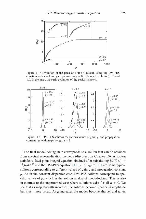
11.2 Power-energy-saturation equation 325
0 200 400 600 800 1000
5
10
15
20
Z
|U0|
g = 0.1
g = 0.3g = 1.0
g = 0.1g = 0.3
g = 1.0
0
Figure 11.7 Evolution of the peak of a unit Gaussian using the DM-PESequation with s = 1 and gain parameters g = 0.1 (damped evolution), 0.3 and1.0. In the inset, the early evolution of the peaks is shown.
−10 0 100
2
4
6
8
10
|U0|
s = 0.1
g = 0.3
μ = 17.10g = 0.7
μ = 44.0
μ = 1.55
g = 1.0
−10 0 100
2
4
6
8
10
t
s = 1.0
μ = 72
μ = 33
g = 1.0
μ = 0.66g = 0.3
g = 0.7
−50 0 500
0.5
1
1.5
2
2.5
s = 10
μ = 3.93g = 1.0
μ = 1.24g = 0.7
μ = 0.13g = 0.3
Figure 11.8 DM-PES solitons for various values of gain, g, and propagationconstant, μ, with map strength s = 1.
The final mode-locking state corresponds to a soliton that can be obtainedfrom spectral renormalization methods (discussed in Chapter 10). A solitonsatisfies a fixed point integral equation obtained after substituting U0(Z, ω) →U0(ω)eiμZ into the DM-PES equation (11.3). In Figure 11.8 are some typicalsolitons corresponding to different values of gain g and propagation constantμ. As in the constant dispersive case, DM-PES solitons correspond to spe-cific values of μ, which is the soliton analog of mode-locking. This is alsoin contrast to the unperturbed case where solutions exist for all μ > 0. Wesee that as map strength increases the solitons become smaller in amplitudebut much more broad. As μ increases the modes become sharper and taller.
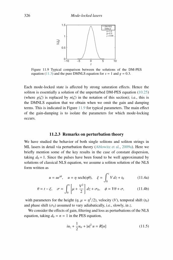
326 Mode-locked lasers
−10
1.5
1
0.5
0−5 0 5 10
t
DM-PESDMNLS
s = 1.0g = 0.3μ = 0.66
|U0|
Figure 11.9 Typical comparison between the solutions of the DM-PESequation (11.3) and the pure DMNLS equation for s = 1 and g = 0.3.
Each mode-locked state is affected by strong saturation effects. Hence thesoliton is essentially a solution of the unperturbed DM-PES equation (10.25)(where g(ζ) is replaced by n(ζ) in the notation of this section); i.e., this isthe DMNLS equation that we obtain when we omit the gain and dampingterms. This is indicated in Figure 11.9 for typical parameters. The main effectof the gain-damping is to isolate the parameters for which mode-lockingoccurs.
11.2.3 Remarks on perturbation theory
We have studied the behavior of both single solitons and soliton strings inML lasers in detail via perturbation theory (Ablowitz et al., 2009a). Here webriefly mention some of the key results in the case of constant dispersion,taking d0 = 1. Since the pulses have been found to be well approximated bysolutions of classical NLS equation, we assume a soliton solution of the NLSform written as
u = ueiφ, u = η sech(ηθ), ξ =
∫ z
0V dz + t0 (11.4a)
θ = t − ξ, σ =
∫ z
0
[μ +
V2
2
]dz + σ0, φ = Vθ + σ, (11.4b)
with parameters for the height (η, μ = η2/2), velocity (V), temporal shift (t0)and phase shift (σ0) assumed to vary adiabatically, i.e., slowly, in z.
We consider the effects of gain, filtering and loss as perturbations of the NLSequation, taking d0 = n = 1 in the PES equation,
iuz +12
utt + |u|2 u = R[u] (11.5)
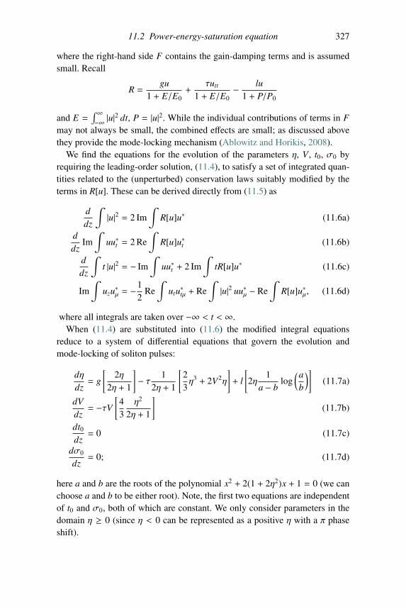
11.2 Power-energy-saturation equation 327
where the right-hand side F contains the gain-damping terms and is assumedsmall. Recall
R =gu
1 + E/E0+
τutt
1 + E/E0− lu
1 + P/P0
and E =∫ ∞−∞ |u|2 dt, P = |u|2. While the individual contributions of terms in F
may not always be small, the combined effects are small; as discussed abovethey provide the mode-locking mechanism (Ablowitz and Horikis, 2008).
We find the equations for the evolution of the parameters η, V , t0, σ0 byrequiring the leading-order solution, (11.4), to satisfy a set of integrated quan-tities related to the (unperturbed) conservation laws suitably modified by theterms in R[u]. These can be derived directly from (11.5) as
ddz
∫|u|2 = 2 Im
∫R[u]u∗ (11.6a)
ddz
Im∫
uu∗t = 2 Re∫
R[u]u∗t (11.6b)
ddz
∫t |u|2 = − Im
∫uu∗t + 2 Im
∫tR[u]u∗ (11.6c)
Im∫
uzu∗μ = −
12
Re∫
utu∗tμ + Re
∫|u|2 uu∗μ − Re
∫R[u]u∗μ, (11.6d)
where all integrals are taken over −∞ < t < ∞.When (11.4) are substituted into (11.6) the modified integral equations
reduce to a system of differential equations that govern the evolution andmode-locking of soliton pulses:
dηdz= g
[2η
2η + 1
]− τ 1
2η + 1
[23η3 + 2V2η
]+ l
[2η
1a − b
log(ab
)](11.7a)
dVdz= −τV
[43
η2
2η + 1
](11.7b)
dt0dz= 0 (11.7c)
dσ0
dz= 0; (11.7d)
here a and b are the roots of the polynomial x2 + 2(1 + 2η2)x + 1 = 0 (we canchoose a and b to be either root). Note, the first two equations are independentof t0 and σ0, both of which are constant. We only consider parameters in thedomain η ≥ 0 (since η < 0 can be represented as a positive η with a π phaseshift).
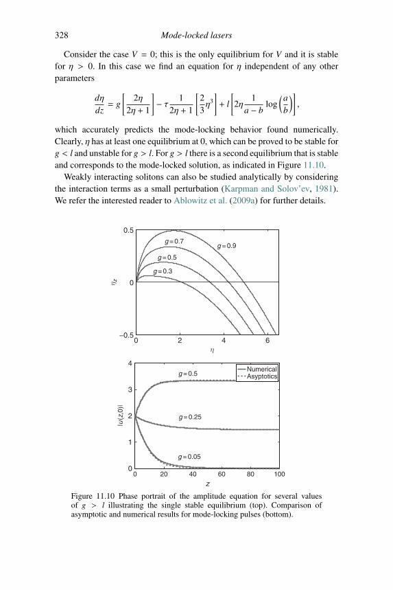
328 Mode-locked lasers
Consider the case V = 0; this is the only equilibrium for V and it is stablefor η > 0. In this case we find an equation for η independent of any otherparameters
dηdz= g
[2η
2η + 1
]− τ 1
2η + 1
[23η3
]+ l
[2η
1a − b
log(ab
)],
which accurately predicts the mode-locking behavior found numerically.Clearly, η has at least one equilibrium at 0, which can be proved to be stable forg < l and unstable for g > l. For g > l there is a second equilibrium that is stableand corresponds to the mode-locked solution, as indicated in Figure 11.10.
Weakly interacting solitons can also be studied analytically by consideringthe interaction terms as a small perturbation (Karpman and Solov’ev, 1981).We refer the interested reader to Ablowitz et al. (2009a) for further details.
0 2 4 6−0.5
0
0.5
η
η z
g = 0.3
g = 0.5
g = 0.7g = 0.9
0 20 40 60 80 1000
1
2
3
4
z
|u(z
,0)|
NumericalAsyptoticsg = 0.5
g = 0.25
g = 0.05
Figure 11.10 Phase portrait of the amplitude equation for several valuesof g > l illustrating the single stable equilibrium (top). Comparison ofasymptotic and numerical results for mode-locking pulses (bottom).
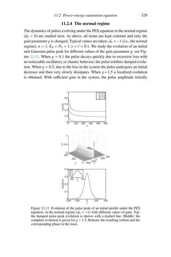
11.2 Power-energy-saturation equation 329
11.2.4 The normal regime
The dynamics of pulses evolving under the PES equation in the normal regime(d0 < 0) are studied next. As above, all terms are kept constant and only thegain parameter g is changed. Typical values are taken: d0 = −1 (i.e., the normalregime), n = 1, E0 = P0 = 1, τ = l = 0.1. We study the evolution of an initialunit Gaussian pulse peak for different values of the gain parameter g; see Fig-ure 11.11. When g = 0.1 the pulse decays quickly due to excessive loss withno noticeable oscillatory or chaotic behavior; the pulse exhibits damped evolu-tion. When g = 0.5, due to the loss in the system the pulse undergoes an initialdecrease and then very slowly dissipates. When g= 1.5 a localized evolutionis obtained. With sufficient gain in the system, the pulse amplitude initially
0 100 200 300 400 5000
0.2
0.4
0.6
0.8
1
z
|u(z
,0)|
g = 0.1g = 0.5g = 1.5
−5000
−250250
500
0
200
4000
0.5
1
tz
|u|
−500 0 500250−2500
0.1
0.2
0.3
0.4
t
|u(4
00,t
)| −500 0 5000
400
t
phas
e
Figure 11.11 Evolution of the pulse peak of an initial profile under the PESequation, in the normal regime (d0 = −1) with different values of gain. Top:the damped pulse-peak evolution is shown with a dashed line. Middle: thecomplete evolution is given for g = 1.5. Bottom: the resulting soliton and thecorresponding phase in the inset.
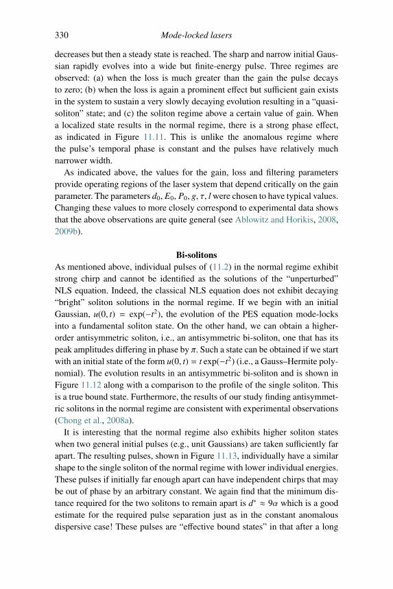
330 Mode-locked lasers
decreases but then a steady state is reached. The sharp and narrow initial Gaus-sian rapidly evolves into a wide but finite-energy pulse. Three regimes areobserved: (a) when the loss is much greater than the gain the pulse decaysto zero; (b) when the loss is again a prominent effect but sufficient gain existsin the system to sustain a very slowly decaying evolution resulting in a “quasi-soliton” state; and (c) the soliton regime above a certain value of gain. Whena localized state results in the normal regime, there is a strong phase effect,as indicated in Figure 11.11. This is unlike the anomalous regime wherethe pulse’s temporal phase is constant and the pulses have relatively muchnarrower width.
As indicated above, the values for the gain, loss and filtering parametersprovide operating regions of the laser system that depend critically on the gainparameter. The parameters d0, E0, P0, g, τ, l were chosen to have typical values.Changing these values to more closely correspond to experimental data showsthat the above observations are quite general (see Ablowitz and Horikis, 2008,2009b).
Bi-solitonsAs mentioned above, individual pulses of (11.2) in the normal regime exhibitstrong chirp and cannot be identified as the solutions of the “unperturbed”NLS equation. Indeed, the classical NLS equation does not exhibit decaying“bright” soliton solutions in the normal regime. If we begin with an initialGaussian, u(0, t) = exp(−t2), the evolution of the PES equation mode-locksinto a fundamental soliton state. On the other hand, we can obtain a higher-order antisymmetric soliton, i.e., an antisymmetric bi-soliton, one that has itspeak amplitudes differing in phase by π. Such a state can be obtained if we startwith an initial state of the form u(0, t) = t exp(−t2) (i.e., a Gauss–Hermite poly-nomial). The evolution results in an antisymmetric bi-soliton and is shown inFigure 11.12 along with a comparison to the profile of the single soliton. Thisis a true bound state. Furthermore, the results of our study finding antisymmet-ric solitons in the normal regime are consistent with experimental observations(Chong et al., 2008a).
It is interesting that the normal regime also exhibits higher soliton stateswhen two general initial pulses (e.g., unit Gaussians) are taken sufficiently farapart. The resulting pulses, shown in Figure 11.13, individually have a similarshape to the single soliton of the normal regime with lower individual energies.These pulses if initially far enough apart can have independent chirps that maybe out of phase by an arbitrary constant. We again find that the minimum dis-tance required for the two solitons to remain apart is d∗ ≈ 9α which is a goodestimate for the required pulse separation just as in the constant anomalousdispersive case! These pulses are “effective bound states” in that after a long
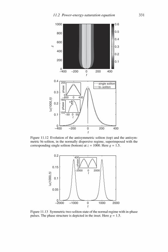
11.2 Power-energy-saturation equation 331
t
z
−200 0 200 400−400
200
400
600
800
1000
0
0.1
0.2
0.3
0.4
0.5
0.6
−400 −200 0 200 4000
0.1
0.2
0.3
0.4
t
|u(1
000,
t)| −400 0 400
0
200
phas
e
−50 0 50155
165
t
phas
e
single solitonbi−soliton
π
Figure 11.12 Evolution of the antisymmetric soliton (top) and the antisym-metric bi-soliton, in the normally dispersive regime, superimposed with thecorresponding single soliton (bottom) at z = 1000. Here g = 1.5.
−2000 −1000 0 1000 20000
0.05
0.1
0.15
0.2
t
|u(1
000,
t)| −2000 0 2000
0
400
t
phas
e
Figure 11.13 Symmetric two-soliton state of the normal regime with in-phasepulses. The phase structure is depicted in the inset. Here g = 1.5.
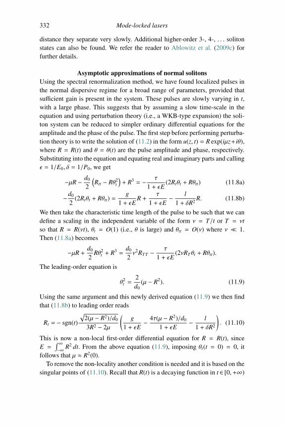
332 Mode-locked lasers
distance they separate very slowly. Additional higher-order 3-, 4-, . . . solitonstates can also be found. We refer the reader to Ablowitz et al. (2009c) forfurther details.
Asymptotic approximations of normal solitonsUsing the spectral renormalization method, we have found localized pulses inthe normal dispersive regime for a broad range of parameters, provided thatsufficient gain is present in the system. These pulses are slowly varying in t,with a large phase. This suggests that by assuming a slow time-scale in theequation and using perturbation theory (i.e., a WKB-type expansion) the soli-ton system can be reduced to simpler ordinary differential equations for theamplitude and the phase of the pulse. The first step before performing perturba-tion theory is to write the solution of (11.2) in the form u(z, t) = R exp(iμz+ iθ),where R = R(t) and θ = θ(t) are the pulse amplitude and phase, respectively.Substituting into the equation and equating real and imaginary parts and callingε = 1/E0, δ = 1/P0, we get
−μR − d0
2
(Rtt − Rθ2
t
)+ R3 = − τ
1 + εE(2Rtθt + Rθtt) (11.8a)
−d0
2(2Rtθt + Rθtt) =
g1 + εE
R +τ
1 + εE− l
1 + δR2R. (11.8b)
We then take the characteristic time length of the pulse to be such that we candefine a scaling in the independent variable of the form ν = T/t or T = νtso that R = R(νt), θt = O(1) (i.e., θ is large) and θtt = O(ν) where ν � 1.Then (11.8a) becomes
−μR +d0
2Rθ2
t + R3 =d0
2ν2RTT − τ
1 + εE(2νRT θt + Rθtt).
The leading-order equation is
θ2t =
2d0
(μ − R2). (11.9)
Using the same argument and this newly derived equation (11.9) we then findthat (11.8b) to leading order reads
Rt = − sgn(t)
√2(μ − R2)/d0
3R2 − 2μ
(g
1 + εE− 4τ(μ − R2)/d0
1 + εE− l
1 + δR2
). (11.10)
This is now a non-local first-order differential equation for R = R(t), sinceE =
∫ ∞−∞ R2 dt. From the above equation (11.9), imposing θt(t = 0) = 0, it
follows that μ ≈ R2(0).To remove the non-locality another condition is needed and it is based on the
singular points of (11.10). Recall that R(t) is a decaying function in t ∈ [0,+∞)
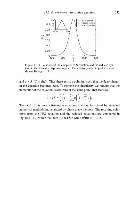
11.2 Power-energy-saturation equation 333
−400 −200 0 200 4000
0.05
0.1
0.15
0.2
0.25
0.3
t
R(t
)
PES equationreduced systemparabolic profile
−500 0 5000
200
t
θ(t)
Figure 11.14 Solutions of the complete PES equation and the reduced sys-tem, in the normally dispersive regime. The relative parabolic profile is alsoshown. Here g = 1.5.
and μ ≈ R2(0) ≥ R(t)2. Thus there exists a point in t such that the denominatorin the equation becomes zero. To remove the singularity we require that thenumerator of the equation is also zero at the same point; that leads to
1 + εE =1l
(g − 2τ
3d0μ
) (1 +
2δ3μ
).
Thus (11.10) is now a first-order equation that can be solved by standardnumerical methods and analyzed by phase plane methods. The resulting solu-tions from the PES equation and the reduced equations are compared inFigure 11.14. Notice that here μ = 0.1216 while R2(0) = 0.1218.
References
Ablowitz, M.J., Bakirtas, I., and Ilan, B. 2005. Wave collapse in nonlocal nonlinearSchrodinger systems. Physica D, 207, 230–253.
Ablowitz, M.J., and Biondini, G. 1998. Multiscale pulse dynamics in communicationsystems with strong dispersion-management. Opt. Lett., 23, 1668–1670.
Ablowitz, M.J., Biondini, G., Biswas, A., Docherty, A., Hirooka, T., and Chakravarty,S. 2002a. Collision-induced timing shifts in dispersion-managed soliton systems.Opt. Lett., 27, 318–320.
Ablowitz, M.J., Biondini, G., and Blair, S. 1997. Multi-dimensional pulse propagationin non-resonant χ(2) materials. Phys. Lett. A, 236, 520–524.
Ablowitz, M.J., Biondini, G., and Blair, S. 2001a. Nonlinear Schrodinger equationswith mean terms in non-resonant multi-dimensional quadratic materials. Phys.Rev. E, 63, 605–620.
Ablowitz, M.J., Biondini, G., Chakravarty, S., and Horne, R.L. 2003a. Four wavemixing in dispersion-managed return-to-zero systems. J. Opt. Soc. Am. B, 20,831–845.
Ablowitz, M.J., Biondini, G., Chakravarty, S., Jenkins, R.B., and Sauer, J.R. 1996.Four-wave mixing in wavelength-division-multiplexed soliton systems: dampingand amplification. Opt. Lett., 21, 1646–1648.
Ablowitz, M.J., Biondini, G., and Olson, E. 2000b. On the evolution and interactionof dispersion-managed solitons. In: Massive WDM and TDM Soliton Trans-mission Systems, edited by Akira Hasegawa. Kyoto, Japan: Kluwer Academic,pp. 362–367.
Ablowitz, M.J., and Clarkson, P.A. 1991. Solitons, Nonlinear Evolution Equations andInverse Scattering. Cambridge: Cambridge University Press.
Ablowitz, M.J., Docherty, A., and Hirooka, T. 2003b. Incomplete collisions instrongly dispersion-managed return-to-zero communication systems. Opt. Lett.,28, 1191–1193.
Ablowitz, M.J., and Fokas, A.S. 2003. Complex Variables: Introduction andApplications. Second edition. Cambridge: Cambridge University Press.
Ablowitz, M.J., Fokas, A.S., and Musslimani, Z. 2006. On a new nonlocal formulationof water waves. J. Fluid Mech., 562, 313–344.
Ablowitz, M.J., and Haberman, R. 1975. Resonantly coupled nonlinear evolutionequations. Phys. Rev. Lett., 38, 1185–1188.
334
References 335
Ablowitz, M.J., Hammack, J., Henderson, D., and Schober, C.M. 2000a. Modulatedperiodic waves in deep water. Phys. Rev. Lett., 84, 887–890.
Ablowitz, M.J., Hammack, J., Henderson, D., and Schober, C.M. 2001. Long timedynamics of the modulational instability of deep water waves. Physica D, 152,416–433.
Ablowitz, M.J., and Haut, T.S. 2009a. Asymptotic expansions for solitary gravity–capillary waves in two and three dimensions. Proc. R. Soc. Lond. A, 465,2725–2749.
Ablowitz, M.J., and Haut, T.S. 2009b. Coupled nonlinear Schrodinger equations frominterfacial fluids with a free surface. Theor. Math. Phys., 159, 689–697.
Ablowitz, M.J., and Haut, T.S. 2010. Asymptotic expansions for solitary gravity-capillary waves in two dimensions. J. Phys. Math Theor., 43, 434005.
Ablowitz, M.J., Hirooka, T., and Biondini, G. 2001b. Quasi-linear optical pulses instrongly dispersion-managed transmission systems. Opt. Lett., 26, 459–461.
Ablowitz, M.J., and Hirooka, T. 2002. Managing nonlinearity in strongly dispersion-managed optical pulse transmission. J. Opt. Soc. Am. B, 19, 425–439.
Ablowitz, M.J., Hirooka, T., and Inoue, T. 2002b. Higher order asymptotic analysisof dispersion-managed transmission systems: solitons and their characteristics.J. Opt. Soc. Am. B, 19, 2876–2885.
Ablowitz, M.J., and Horikis, T.P. 2008. Pulse dynamics and solitons in mode-lockedlasers. Phys. Rev. A, 78, 011802.
Ablowitz, M.J., and Horikis, T.P. 2009a. Solitons and spectral renormalization methodsin nonlinear optics. Eur. Phys. J. Special Topics, 173, 147–166.
Ablowitz, M.J., and Horikis, T.P. 2009b. Solitons in normally dispersive mode-lockedlasers. Phys. Rev. A, 79, 063845.
Ablowitz, M.J., Horikis, T.P., and Ilan, B. 2008. Solitons in dispersion-managed mode-locked lasers. Phys. Rev. A, 77, 033814.
Ablowitz, M.J., Horikis, T.P., and Nixon, S.D. 2009c. Soliton strings and interactionsin mode-locked lasers. Opt. Comm., 282, 4127–4135.
Ablowitz, M.J., Horikis, T.P., Nixon, S.D., and Zhu, Y. 2009a. Asymptotic analysis ofpulse dynamics in mode-locked lasers. Stud. Appl. Math., 122, 411–425.
Ablowitz, M.J., Ilan, B., and Cundiff, S.T. 2004a. Carrier-envelope phase slip ofultra-short dispersion-managed solitons. Opt. Lett., 29, 1818–1820.
Ablowitz, M.J., Kaup, D.J., Newell, A.C., and Segur, H. 1973a. Method for solvingsine–Gordon equation. Phys. Rev. Lett., 30, 1262–1264.
Ablowitz, M.J., Kaup, D.J., Newell, A.C., and Segur, H. 1973b. Nonlinear-evolutionequations of physical significance. Phys. Rev. Lett., 31, 125–127.
Ablowitz, M.J., Kaup, D.J., Newell, A.C., and Segur, H. 1974. Inverse scatter-ing transform—Fourier analysis for nonlinear problems. Stud. Appl. Math., 53,249–315.
Ablowitz, M.J., Kruskal, M.D., and Segur, H. 1979. A note on Miura’s transformation.J. Math. Phys., 20, 999–1003.
Ablowitz, M.J., Manakov, S.V., and Schultz, C.L. 1990. On the boundary conditions ofthe Davey–Stewartson equation. Phys. Lett. A, 148, 50–52.
Ablowitz, M.J., and Musslimani, Z. 2003. Discrete spatial solitions in a diffraction-managed nonlinear waveguide array: a unified approach. Physica D, 184,276–303.
336 References
Ablowitz, M.J., and Musslimani, Z. 2005. Spectral renormalization method for com-puting self-localized solutions to nonlinear systems. Opt. Lett., 30, 2140–2142.
Ablowitz, M.J., Nixon, S.D., and Zhu, Y. 2009b. Conical diffraction in honeycomblattices. Phys. Rev. A, 79, 053830.
Ablowitz, M.J., Prinari, B., and Trubatch, A.D. 2004b. Discrete and ContinuousNonlinear Schrodinger Systems. Cambridge: Cambridge University Press.
Ablowitz, M.J., and Segur, H. 1979. On the evolution of packets of water waves. J. FluidMech., 92, 691–715.
Ablowitz, M.J., and Segur, H. 1981a. Solitons and the Inverse Scattering Transform.Philadelphia: SIAM.
Ablowitz, M.J., and Villarroel, J. 1991. On the Kadomtsev–Petviashili equation andassociated constraints. Stud. Appl. Math., 85, 195–213.
Ablowitz, M.J., and Wang, X.P. 1997. Initial time layers in Kadomtsev–Petviashili typeequations. Stud. Appl. Math., 98, 121–137.
Abramowitz, M., and Stegun, I.R. 1972. Handbook of Mathematical Functions. Tenthedition. New York: Dover.
Agrawal, G.P. 2001. Nonlinear Fiber Optics. New York: Academic Press.Agrawal, G.P. 2002. Fiber-Optic Communication Systems. New York: Wiley-
Interscience.Ahrens, C. 2006. The asymptotic analysis of communications and wave collapse
problems in nonlinear optics. Ph.D. thesis, University of Colorado.Airy, G.B. 1845. Tides and waves. Encyc. Metrop., 192, 241–396.Akhmediev, N.N., and Ankiewicz, A. 1997. Solitons, Nonlinear Pulses and Beams.
London: Chapman & Hall.Akhmediev, N.N., Soto-Crespo, J.M., and Town, G. 2001. Pulsating solitons, chaotic
solitons, period doubling, and pulse coexistence in mode-locked lasers: ComplexGinzburg–Landau equation approach. Phys. Rev. E, 63, 056602.
Alfimov, G.L., Kevrekidis, P.G., Konotop, V.V., and Salerno, M. 2002. Wannierfunctions analysis of the nonlinear Schrodinger equation with a periodic potential.Phys. Rev. E, 66, 046608.
Angulo, J., Bona, J.L., Linares, F., and Scialom, F. 2002. Scaling, stability andsingularities for nonlinear, dispersive wave equations: the critical case. Nonlin-earity, 15, 759–786.
Batchelor, G.K. 1967. An Introduction to Fluid Dynamics. Cambridge: CambridgeUniversity Press.
Beals, R., and Coifman, R.R. 1984. Scattering and inverse scattering for 1st ordersystems. Comm. Pure Appl. Math., 37, 39–90.
Beals, R., and Coifman, R.R. 1985. Inverse scattering and evolution-equations. Comm.Pure Appl. Math., 38, 29–42.
Beals, R., Deift, P., and Tomei, C. 1988. Direct and Inverse Scattering on the Line.Providence, RI: AMS.
Bender, C.M., and Orszag, S.A. 1999. Advanced Mathematical Methods for Scientistsand Engineers. Berlin: Springer.
Benjamin, T.B., and Feir, J.F. 1967. The disintegration of wave trains on deep water.Part 1. Theory. J. Fluid Mech., 27, 417–430.
Benjamin, T.B., Bona, J.L., and Mahony, J.J. 1972. Model equations for long waves innonlinear dispersive systems. Phil. Trans. Roy. Soc. A, 227, 47–78.
References 337
Benney, D.J. 1966a. Long non-linear waves in fluid flows. J. Math. and Phys., 45,52–63.
Benney, D.J. 1966b. Long waves on liquid films. J. Math. and Phys., 45, 150–155.Benney, D.J., and Luke, J.C. 1964. Interactions of permanent waves of finite amplitude.
J. Math. Phys., 43, 309–313.Benney, D.J., and Newell, A.C. 1967. The propagation of nonlinear envelopes. J. Math.
and Phys., 46, 133–139.Benney, D.J., and Roskes, G.J. 1969. Wave instabilities. Stud. Appl. Math., 48, 377–385.Bleistein, N. 1984. Mathematical Methods for Wave Phenomena. New York: Academic
Press.Bleistein, N., and Handelsman, R.A. 1986. Asymptotic Expansions of Integrals.
New York: Dover.Bogoliubov, N.N., and Mitropolsky, Y.A. 1961. Asymptotic Methods in the Theory
of Non-linear Oscillations. Second edition. Russian monographs and texts onadvanced mathematics and physics, vol. 10. London: Taylor & Francis.
Boussinesq, J.M. 1871. Theorie de l’intumescence appelee onde solitaire ou de trans-lation se propageant dans un canal rectangulaire. Comptes Rendues, Acad. Sci.Paris, 72, 755–759.
Boussinesq, J.M. 1872. Theorie des ondes et des remous qui se propagent le long d’uncanal rectangulaire horizontal, en communiquant au liquide contenu dans ce canaldes vitesses sensiblemant parielles de la surface au fond. J. Math. Pures Appl.Ser. (2), 17, 55–108.
Boussinesq, J.M. 1877. Essai sur la theorie des eaux courantes. Memoires presente pardivers savantes a l’Acad. des Sci. Inst. NAT. France XXIII, 1–680.
Boyd, R.W. 2003. Nonlinear Optics. New York: Academic Press.Byrd, P.F., and Friedman, M.D. 1971. Handbook of Elliptic Integrals for Engineers and
Physicists. Berlin: Springer.Calogero, F., and Degasperis, A. 1982. Spectral Transform and Solitons. Amsterdam:
Elsevier.Calogero, F., and DeLillo, S. 1989. The Burgers equation on the semi-infinite and finite
intervals. Nonlinearity, 2, 37–43.Camassa, R., and Holm, D.D. 1993a. An integrable shallow water equation with peaked
solitons. Phys. Rev. Lett., 71, 1661–1664.Camassa, R., and Holm, D.D. 1993b. An integrable shallow water equation with peaked
solitons. Phys. Rev. Lett., 11, 1661–1664.Caudrey, P.J. 1982. The inverse problem for a general N ×N spectral equation. Physica
D, 6, 51–66.Chapman, S., and Cowling, T. 1970. Mathematical Theory of Nonuniform Gases.
Cambridge: Cambridge University Press.Chen, M., Tsankov, M.A., Nash, J.M., and Patton, C.E. 1994. Backward volume
wave microwave envelope solitons in yttrium iron garnet films. Phys. Rev. B, 49,12773–12790.
Chester, C., Friedman, B., and Ursell, F. 1957. An extension of the method of steepestdescents. Proc. Camb. Phil. Soc., 53, 599–611.
Chong, A., Renninger, W.H., and Wise, F.W. 2008a. Observation of antisymmetricdispersion-managed solitons in a mode-locked laser. Opt. Lett., 33, 1717–1719.
Chong, A., Renninger, W.H., and Wise, F.W. 2008b. Properties of normal-dispersionfemtosecond fiber lasers. J. Opt. Soc. Am. B, 25, 140–148.
338 References
Christodoulides, D.N., and Joseph, R.I. 1998. Discrete self-focusing in nonlinear arraysof coupled waveguides. Opt. Lett., 13(9), 794–796.
Clarkson, P.A., Fokas, A.S., and Ablowitz, M.J. 1989. Hodograph transformations oflinearizable partial differential equations. SIAM J. Appl. Math., 49, 1188–1209.
Cole, J.D. 1951. On a quasilinear parabolic equation occurring in aerodynamics. Quart.Appl. Math., 9, 225–236.
Cole, J.D. 1968. Perturbation Methods in Applied Mathematics. London: Ginn and Co.Copson, E.T. 1965. Asymptotic Expansions. Cambridge: Cambridge University Press.Courant, R., Friedrichs, K., and Lewy, H. 1928. On the partial differential equations of
mathematical physics. Math. Ann., 100, 32–74. English Translation, IBM Journal,11:215–234, 1967.
Courant, R., and Hilbert, D. 1989. Methods of Mathematical Physics. New York: JohnWiley.
Craig, W., and Groves, M.D. 1994. Hamiltonian long-wave approximations to thewater-wave problem. Wave Motion, 19, 367–389.
Craig, W., and Sulem, C. 1993. Numerical simulation of gravity-waves. J. Comp. Phys.,108, 73–83.
Crasovan, L.C., Torres, J.P., Mihalache, D., and Torner, L. 2003. Arresting wavecollapse by self-rectification. Phys. Rev. Lett., 9, 063904.
Cundiff, S.T. 2005. Soliton dynamics in mode-locked lasers. Lect. Notes Phys., 661,183–206.
Cundiff, S.T., Ye, J., and Hall, J. 2008. Rulers of light. Scientific American, April,74–81.
Davey, A., and Stewartson, K. 1974. On three dimensional packets of surface waves.Proc. Roy. Soc. London A, 338, 101–110.
Deift, P., and Trubowitz, E. 1979. Inverse scattering on the line. Comm. Pure Appl.Math., 32, 121–251.
Deift, P., Venakides, S., and Zhou, X. 1994. The collisionless shock region for the long-time behavior of solutions of the KdV equation. Comm. Pure Appl. Math., 47,199–206.
Deift, P., and Zhou, X. 1992. A steepest descent method for oscillatory Riemann–Hilbert problems. Bull. Amer. Math. Soc., 26, 119–123.
Dickey, L.A. 2003. Soliton Equations and Hamiltonian Systems. Singapore: WorldScientific.
Djordjevic, V.D., and Redekopp, L.G. 1977. On two-dimensional packets of capillary–gravity waves. J. Fluid Mech., 79, 703–714.
Docherty, A. 2003. Collision induced timing shifts in wavelength-division-multiplexedoptical fiber communications systems. Ph.D. thesis, University of New SouthWales.
Dodd, R.K., Eilbeck, J.C., Gibbon, J.D., and Morris, H.C. 1984. Solitons and NonlinearWave Equations. New York: Academic Press.
Douxois, T. 2008. Fermi–Pasta–Ulam and a mysterious lady, Physics Today, Jan. 2008,55–57.
Dysthe, K.B. 1979. Note on a modification to the nonlinear Schrodinger equation forapplication to deep water waves. Proc. Roy. Soc. London A, 369, 105–114.
Elgin, J.N. 1985. Inverse scattering theory with stochastic initial potentials. Phys.Lett. A, 110, 441–443.
Erdelyi, A. 1956. Asymptotic Expansions. New York: Dover.
References 339
Faddeev, L.D. 1963. The inverse problem in the quantum theory of scattering. J. Math.Phys., 4, 72–104.
Faddeev, L.D., and Takhtajan, L.A. 1987. Hamiltonian Methods in the Theory ofSolitons. Berlin: Springer.
Falcon, E., Laroche, C., and Fauve, S. 2002. Observation of depression solitary surfacewaves on a thin fluid layer. Phys. Rev. Lett., 89, 204501.
Fermi, E., Pasta, S., and Ulam, S. 1955. Studies of nonlinear problems, I. Tech. rept.Los Alamos Report LA1940. [Reproduced in ”Nonlinear Wave Motion,” proceed-ings, Potsdam, New York, 1972, ed. A.C. Newell, Lect. Appl. Math., 15, 143–156,A.M.S., Providence, RI, (1974).].
Fibich, G., and Papanicolaou, G. 1999. Self-focusing in the perturbed and unperturbednonlinear Schrodinger equation in critical dimension. SIAM J. App. Math., 60,183–240.
Fokas, A.S. 2008. A Unified Approach to Boundary Value Problems. Philadelphia:SIAM.
Fokas, A.S., and Anderson, R.L. 1982. On the use of isospectral eigenvalue problemsfor obtaining hereditary symmetries for Hamiltonian-systems. J. Math. Phys., 23,1066–1073.
Fokas, A.S., and Fuchssteiner, B. 1981. Symplectic structures, their Backlund transfor-mations and hereditary symmetries. Physica D, 4, 47–66.
Fokas, A.S., and Santini, P.M. 1989. Coherent structures in multidimensions. Phys. Rev.Lett., 63, 1329–1333.
Fokas, A.S., and Santini, P.M. 1990. Dromions and a boundary value problem for theDavey–Stewartson I equation. Physica D, 44, 99–130.
Forsyth, A.R. 1906. Theory of Differential Equations. Part IV—Partial DifferentialEquations. Cambridge: Cambridge University Press.
Gabitov, I.R., and Turitsyn, S.K. 1996. Averaged pulse dynamics in a cascadedtransmission system with passive dispersion compensation. Opt. Lett., 21,327–329.
Garabedian, P. 1984. Partial Differential Equations. New York: Chelsea.Gardner, C.S., Greene, J., Kruskal, M., and Miura, R.M. 1967. Method for solving the
Korteweg–de Vries equation. Phys. Rev. Lett., 19, 1095–1097.Gardner, C.S., and Su, C.S. 1969. The Korteweg–de Vries equation and generalizations.
III. J. Math. Phys., 10, 536–539.Gardner, C.S., Greene, J.M., Kruskal, M.D., and Miura, R.M. 1974. Korteweg–de Vries
and generalizations. VI. Methods for exact solution. Commun. Pure Appl. Math.,27, 97–133.
Gel’fand, I.M., and Dickii, L.A. 1977. Resolvants and Hamiltonian systems. Func.Anal. Appl., 11, 93–104.
Goldstein, H. 1980. Classical Mechanics. Reading, MA: Addison Wesley.Gordon, J.P., and Haus, H.A. 1986. Random walk of coherently amplified solitons in
optical fiber transmission. Opt. Lett., 11, 665–667.Hasegawa, A., and Kodama, Y. 1991a. Guiding-center soliton. Phys. Rev. Lett., 66,
161–164.Hasegawa, A., and Kodama, Y. 1991b. Guiding-center soliton in fibers with periodically
varying dispersion. Opt. Lett., 16, 1385–1387.
340 References
Hasegawa, A., and Kodama, Y. 1995. Solitons in Optical Communications. Oxford:Oxford University Press.
Hasegawa, A., and Matsumoto, M. 2002. Optical Solitons in Fibers. Berlin: Springer.Hasegawa, A., and Tappert, F. 1973a. Transmission of stationary nonlinear optical
pulses in dispersive dielectric fibres. I. Anomalous dispersion. Appl. Phys. Lett.,23, 142–144.
Hasegawa, A., and Tappert, F. 1973b. Transmission of stationary nonlinear opticalpulses in dispersive dielectric fibres. II. Normal dispersion. Appl. Phys. Lett., 23,171–172.
Haus, H.A. 1975. Theory of mode locking with a fast saturable absorber. J. Appl. Phys.,46, 3049–3058.
Haus, H.A. 2000. Mode-locking of lasers. IEEE J. Sel. Topics Q. Elec., 6, 1173–1185.Haus, H.A., Fujimoto, J.G., and Ippen, E.P. 1992. Analytic theory of additive pulse and
Kerr lens mode locking. IEEE J. Quant. Elec., 28, 2086–2096.Haut, T.S., and Ablowitz, M.J. 2009. A reformulation and applications of interfacial
fluids with a free surface. J. Fluid Mech., 631, 375–396.Hopf, E. 1950. The partial differential equation ut + uux = μuxx. Comm. Pure Appl.
Math., 3, 201–230.Ilday, F.O., Buckley, J.R., Clark, W.G., and Wise, F.W. 2004b. Self-similar evolution of
parabolic pulses in a laser. Phys. Rev. Lett., 92, 213901.Ilday, F.O., Wise, F.W., and Kaertner, F.X. 2004a. Possibility of self-similar pulse
evolution in a Ti:sapphire laser. Opt. Express, 12, 2731–2738.Infeld, E., and Rowlands, G. 2000. Nonlinear Waves, Solitons and Chaos. Cambridge:
Cambridge University Press.Ishimori, Y. 1981. On the modified Korteweg–deVries soliton and the loop soliton.
J. Phys. Soc. Jpn., 50, 2471–2472.Ishimori, Y. 1982. A relationship between the Ablowitz–Kaup–Newell–Segur and
Wadati–Konno–Ichikawa schemes of the inverse scattering method. J. Phys. Soc.Jpn., 51, 3036–3041.
Jackson, J.D. 1998. Classical Electrodynamics. New York: John Wiley.Jeffreys, H., and Jeffreys, B.S. 1956. Methods of Mathematical Physics. Cambridge:
Cambridge University Press.Kadomtsev, B.B., and Petviashvili, V.I. 1970. On the stability of solitary waves in
weakly dispersive media. Sov. Phys. Doklady, 15, 539–541.Kalinikos, B.A., Kovshikov, N.G., and Patton, C.E. 1997. Decay free microwave enve-
lope soliton pulse trains in yttrium iron garnet thin films. Phys. Rev. Lett., 78,2827–2830.
Kalinikos, B.A., Scott, M.M., and Patton, C.E. 2000. Self generation of fundamentaldark solitons in magnetic films. Phys. Rev. Lett., 84, 4697–4700.
Kapitula, T., Kutz, J.N., and Sandstede, B. 2002. Stability of pulses in the master mode-locking equation. J. Opt. Soc. Am. B, 19, 740–746.
Karpman, V.I., and Solov’ev, V.V. 1981. A perturbation theory for soliton systems.Physica D, 3, 142–164.
Kay, I., and Moses, H.E. 1956. Reflectionless transmission through dielectrics andscattering potentials. J. Appl. Phys., 27, 1503–1508.
Kevorkian, J., and Cole, J.D. 1981. Perturbation Methods in Applied Mathematics.Berlin: Springer.
References 341
Konno, K., and Jeffrey, A. 1983. Some remarkable properties of two loop solitonsolutions. J. Phys. Soc. Jpn., 52, 1–3.
Konopelchenko, B.G. 1993. Solitons in Multidimensions. Singapore: World Scientific.Korteweg, D., and de Vries, G. 1895. On the change of a form of long waves advancing
in a rectangular canal and a new type of long stationary waves. Phil. Mag., 5th
Series, 422–443.Kruskal, M.D. 1963. Asymptotology. In: Proceedings of Conference on Mathemati-
cal Models on Physical Sciences, edited by S. Drobot. Upper Saddle River, NJ:Prentice-Hall.
Kruskal, M.D. 1965. Asymptotology in numerical computation: Progress and planson the Fermi–Pasta–Ulam problem. In: IBM Scientific Computing Symposium onLarge-Scale Problems in Physics, pp. 43–62
Krylov, N.M., and Bogoliubov, N.N. 1949. Introduction to Non-Linear Mechanics.Annals of Mathematics Studies, vol. 11. Princeton: Princeton University Press.
Kutz, J.N. 2006. Mode-locked soliton lasers. SIAM Rev., 48, 629–678.Kuzmak, G.E. 1959. Asymptotic solutions of nonlinear second order differential
equations with variable coefficients. PMM, 23(3), 515–526.Lamb, H. 1945. Hydrodynamics. New York: Dover.Landau, L.D., and Lifshitz, L.M. 1981. Quantum Mechanics: Non-relativistic Theory.
London: Butterworth–Heinemann.Landau, L.D., Lifshitz, E.M., and Pitaevskii, L.P. 1984. Electrodynamics of Continuous
Media. London: Butterworth–Heinemann.Lax, P.D. 1968. Integrals of nonlinear equations of evolution and solitary waves.
Commun. Pure Appl. Math., 21, 467–490.Lax, P.D. 1987. Hyperbolic Systems of Conservation Laws and the Mathematical
Theory of Shock Waves. Philadelphia: SIAM.Lax, P.D., and Levermore, C.D. 1983a. The small dispersion limit of the Korteweg–de
Vries equation. III. Commun. Pure Appl. Math., 36, 809–829.Lax, P.D., and Levermore, C.D. 1983b. The small dispersion limit of the Korteweg–de
Vries equation. I. Commun. Pure Appl. Math., 36, 253–290.Lax, P.D., and Levermore, C.D. 1983c. The small dispersion limit of the Korteweg–de
Vries equation. II. Commun. Pure Appl. Math., 36, 571–593.LeVeque, R.J. 2002. Finite Volume Methods for Hyperbolic Problems. Cambridge:
Cambridge University Press.Lighthill, M.J. 1958. Introduction to Fourier Analysis and Generalized Functions.
Cambridge: Cambridge University Press.Lighthill, M.J. 1978. Waves in Fluids. Cambridge: Cambridge University Press.Lin, C., Kogelnik, H., and Cohen, L.G. 1980. Optical-pulse equalization of low-
dispersion transmission in single-mode fibers in the 1.3–1.7μm spectral region.Opt. Lett., 5, 476–478.
Luke, J.C. 1966. A perturbation method for nonlinear dispersive wave problems. Proc.R. Soc. Lond. A, 292, 403–412.
Lushnikov, P.M. 2001. dispersion-managed solitons in the strong dispersion map limit.Opt. Lett., 26, 1535–1537.
Mamyshev, P.V., and Mollenauer, L.F. 1996. Pseudo-phase-matched four-wave mix-ing in soliton wavelength-division multiplexing transmission. Opt. Lett., 21,396–398.
342 References
Marchenko, V.A. 1986. Sturm–Liouville Operators and Applications. Basel:Birkhauser.
Maruta, A., Inoue, T., Nonaka, Y., and Yoshika, Y. 2002. Bi-solitons propagating indispersion-managed transmission systems. IEEE J. Sel. Top. Quant. Electron., 8,640–650.
Matveev, V.B., and Salle, M.A. 1991. Darboux Transformations and Solitons. Berlin:Springer.
Melin, A. 1985. Operator methods for inverse scattering on the real line. Commun. Part.Diff. Eqns., 10, 677–766.
Merle, F. 2001. Existence of blow-up solutions in the energy space for the criticalgeneralized KdV equation. J. Amer. Math. Soc., 14, 555–578.
Mikhailov, A.V. 1979. Integrability of a two-dimensional generalization of the Todachain. Sov. Phys. JETP Lett., 30, 414–418.
Mikhailov, A.V. 1981. The reduction problem and the inverse scattering method.Physica D, 3, 73–117.
Miles, J.W. 1981. The Korteweg–de Vries equation: An historical essay. J. Fluid Mech.,106 (focus issue), 131–147.
Miura, R.M. 1968. Korteweg–de Vries equation and generalizations. I. A remarkableexplicit nonlinear transformation. J. Math. Phys., 9, 1202–1204.
Miura, R.M., Gardner, C.S., and Kruskal, M.D. 1968. Korteweg–de Vries equationsand generalizations. II. Existence of conservation laws and constants of motion.J. Math. Phys., 9, 1204–1209.
Mollenauer, L.F., Evangelides, S.G., and Gordon, J.P. 1991. Wavelength division multi-plexing with solitons in ultra-long distance transmission using lumped amplifiers.J. Lightwave Technol., 9, 362–367.
Molleneauer, L.F., and Gordon, J.P. 2006. Solitons in Optical Fibers: Fundamentalsand Applications to Telecommunications. New York: Academic Press.
Mollenauer, L.F., Stolen, R.H., and Gordon, J.P. 1980. Experimental observation ofpicosecond pulse narrowing and solitons in optical fibers. Phys. Rev. Lett., 45,1095–1098.
Newell, A.C. 1978. The general structure of integrable evolution equations. Proc. Roy.Soc. Lond. A., 365, 283–311.
Newell, A.C. 1985. Solitons in Mathematics and Physics. Philadelphia: SIAM.Nijhof, J.H.B., Doran, N.J., Forysiak, W., and Knox, F.M. 1997. Stable soliton-like
propagation in dispersion-managed systems with net anomalous, zero and normaldispersion. Electron. Lett., 33, 1726–1727.
Nijhof, J.H.B., Forysiak, W., and Doran, N.J. 2002. The averaging method for findingexactly periodic dispersion-managed solitons. IEEE J. Sel. Topics Q. Elec., 6,330–336.
Novikov, S.P., Manakov, S.V., Pitaevskii, L.P., and Zakharov, V.E. 1984. Theory ofSolitons: The Inverse Scattering Method. New York: Plenum.
Ostrovsky, L.A., and Potapov, A.S. 1986. Modulated Waves: Theory and Applications.Baltimore: The John Hopkins University Press.
Papanicolaou, G., Sulem, C., Sulem, P.L., and Wang, X.-P. 1994. The focusingsingularity of the Davey-Stewartson equations for gravity-capillary surface waves.Physica D, 72, 61–86.
References 343
Patton, C.E., Kabos, P., Xia, H., Kolodin, P.A., Zhang, H.Y., Staudinger, R., Kalinikos,B.A., and Kovshikov, N.G. 1999. Microwave magnetic envelope solitons in thinferrite films. J. Mag. Soc. Japan, 23, 605–610.
Pelinovsky, D.E., and Stepanyants, Y.A. 2004. Convergence of Petviashvili’s iterationmethod for numerical approximation of stationary solutions of nonlinear waveequations. SIAM J. Numer. Anal., 42, 1110–1127.
Pelinovsky, D.E., and Sulem, C. 2000. Spectral decomposition for the Dirac systemassociated to the DSII equation. Inverse Problems, 16, 59–74.
Petviashvili, V.I. 1976. Equation of an extraordinary soliton. Sov. J. Plasma Phys., 2,257–258.
Phillips, O.M. 1977. The Dynamics of the Upper Ocean. Cambridge: CambridgeUniversity Press.
Prinari, B., Ablowitz, M.J., and Biondini, G. 2006. Inverse scattering for the vectornonlinear Schrodinger equation with non-vanishing boundary conditions. J. Math.Phys., 47, 1–33.
Quraishi, Q., Cundiff, S.T., Ilan, B., and Ablowitz, M.J. 2005. Dynamics of nonlinearand dispersion-managed solitons. Phys. Rev. Lett., 94, 243904.
Rabinovich, M.I., and Trubetskov, D.I. 1989. Oscillations and Waves in Linear andNonlinear Systems. Dordsecht: Kluwer Academic.
Rayleigh, Lord. 1876. On waves. Phil. Mag., 1, 257–279.Remoissenet, M. 1999. Waves Called Solitons. Berlin: Springer.Rogers, C., and Schief, W.K. 2002. Backlund and Darboux Transformations.
Cambridge: Cambridge University Press.Russell, J.S. 1844. Report on Waves. In: Report of the 14th meeting of the British
Association for the Advancement of Science. London: John Murray, pp. 311–390.Sanders, J.A., Verhulst, F., and Murdock, J. 2009a. Averaging Methods in Nonlinear
Dynamical Systems. Berlin: Springer.Sanders, M.Y., Birge, J., Benedick, A., Crespo, H.M., and Kartner, F.X. 2009b. Dynam-
ics of dispersion-managed octave-spanning titanium: sapphire lasers. J. Opt. Soc.Am. B, 26, 743–749.
Satsuma, J., and Ablowitz, M.J. 1979. Two-dimensional lumps in nonlinear dispersivesystems. J. Math. Phys., 20, 1496–1503.
Shimizu, T., and Wadati, M. 1980. A new integrable nonlinear evolution equation. Prog.Theor. Phys., 63, 808–820.
Stokes, G.G. 1847. On the theory of oscillatory waves. Camb. Trans., 8, 441–473.Sulem, C., and Sulem, P. 1999. The Nonlinear Schrodinger Equation: Self-Focusing
and Wave Collapse. Berlin: Springer.Tang, D.Y., Man, W.S., Tam, H.Y., and Drummond, P.D. 2001. Observation of bound
states of solitons in a passively mode-locked fiber laser. Phys. Rev. A, 64, 033814.Taniuti, T., and Wei, C.C. 1968. Reductive perturbation method in nonlinear wave
propagation I. J. Phys. Soc. Japan, 24, 941–946.Taylor, G.I. 1950. The formation of a blast wave by a very intense explosion.
I. Theoretical Discussion. Proc. Roy. Soc. A, 201, 159–174.Tsankov, M.A., Chen, M., and Patton, C.E. 1994. Forward volume wave microwave
envelope solitons in yttrium iron garnet films-propagation, decay, and collision.J. Appl. Phys., 76, 4274–4289.
344 References
Venakides, S. 1985. The zero dispersion limit of the Korteweg–de Vries equationfor initial potentials with non-trivial reflection coefficient. Commun. Pure Appl.Math., 38, 125–155.
Villarroel, J., and Ablowitz, M.J. 2002. The Cauchy problem for the Kadomtsev–Petviashili II equation with nondecaying data along a line. Stud. Appl. Math, 109,151–162.
Villarroel, J., and Ablowitz, M.J. 2003. On the discrete spectrum of systems in the planeand the Davey-Stewartson II equation. SIAM J. Math. Anal., 34, 1253–1278.
Vlasov, S., Petrishchev, V., and Talanov, V. 1970. Averaged description of wave beamsin linear and nonlinear media. Radiophys. Quantum Electronics, 14, 1062.
Wadati, M. 1974. The modified Korteweg–de Vries equation. J. Phys. Soc. Jpn., 34,1289–1296.
Wadati, M., Konno, K., and Ichikawa, Y.-H. 1979a. A generalization of inversescattering method. J. Phys. Soc. Jpn., 46, 1965–1966.
Wadati, M., Konno, K., and Ichikawa, Y.H. 1979b. New integrable nonlinear evolutionequations. J. Phys. Soc. Jpn., 47, 1698–1700.
Wadati, M., and Sogo, K. 1983. Gauge transformations in soliton theory. J. Phys. Soc.Jpn., 52, 394–398.
Weinstein, M. 1983. Nonlinear Schrodinger equations and sharp interpolation esti-mates. Comm. Math. Phys., 87, 567–576.
Whitham, G.B. 1965. Non-linear dispersive waves. Proc. R. Soc. Lond. A, 6, 238–261.Whitham, G.B. 1974. Linear and Nonlinear Waves. New York: John Wiley.Wu, M., Kalinikos, B.A., and Patton, C.E. 2004. Generation of dark and bright spin
wave envelope soliton trains through self-modulational instability in magneticfilms. Phys. Rev. Lett., 93, 157207.
Yang, T., and Kath, W.L. 1997. Analysis of enhanced-power solitons in dispersion-managed optical fibers. Opt. Lett., 22, 985–987.
Zabusky, N.J., and Kruskal, M.D. 1965. Interactions of “solitons” in a collisionlessplasma and the recurrence of initial states. Phys. Rev. Lett., 15, 240–243.
Zakharov, V.E. 1968. Stability of periodic waves of finite amplitude on the surface of adeep fluid. Sov. Phys. J. Appl. Mech. Tech. Phys., 4, 190–194.
Zakharov, V.E., and Rubenchik, A.M. 1974. Instability of waveguides and solitons innonlinear media. Sov. Phys. JETP, 38, 494–500.
Zakharov, V.E., and Shabat, A. 1972. Exact theory of two-dimensional self-focusingand one-dimensional self-modulation of waves in a non-linear media. Sov. Phys.JETP, 34, 62–69.
Zakharov, V.E., and Shabat, A.B. 1973. Interaction between solitons in a stable medium.Sov. Phys. JETP, 37, 823–828.
Zharnitsky, V., Grenier, E., Turitsyn, S.K., Jones, C., and Hesthaven, J.S. 2000. Groundstates of dispersion-managed nonlinear Schrodinger equation. Phys. Rev. E, 62,7358–7364.
Zhou, X. 1989. Direct and inverse scattering transforms with arbitrary spectral singu-larities. Commun. Pure Appl. Math., 42, 95–938.
Zvezdin, A.K., and Popkov, A.F. 1983. Contribution to the nonlinear theory ofmagnetostatic spin waves. Sov. Phys. JETP., 51, 350–354.
Index
Abel integral equation, 72adiabatic invariant, 87, 89admissibility conditions, 29Airy function, 55, 59, 60Airy’s equation, 59AKNS method, 201anomalous dispersion, 314, 319associated flux, 194asymptotic expansion, 49asymptotic sequence, 49averaged equation, 324
Benney–Luke equation, 127KP equation, 128with surface tension, 127
Benney–Roskes equations, see BR equationsBernoulli equation, 101bi-soliton, 330blow-up, 163, 317bound state, 245Boussinesq equation, 5, 15, 109, 167, 210
linearized, 109Boussinesq model
coupled, 110BR equations, 158, 165, 182breaking time, 26Burgers’ equation, 30, 199
generalized, 32inviscid, 6, 21, 26, 32, 71linearized, 73semi-infinite interval, 71viscous, 27, 31, 68
Camassa–Holm equation, 212centro-symmetric material, 171CFL condition, 68
channel, wavelength, 303characteristics, 36, 37characteristics, method of, 25, 26chirp, 289, 314, 330cnoidal function, 13, 120cnoidal wave, 8Cole–Hopf transformation, 68, 197collison-induced time shift, 262conservation law, 23, 194conservation of wave equation, 52conserved density, 194convective derivative, 100convolution theorem, 42CW, 266CW wave, 179
D’Alembert’s solution to wave equation, 36,43
Davey–Stewartson (DS) equation, 159generalized, (GDS), 159
deep-water dispersion relationship, 104deep-water limit, 148density of a conserved quantity, 23direct scattering problem, 198, 214Dirichlet–Neumann map methods, 124Dirichlet–Neumann relationship, 71discrete eigenvalue, see eigenvalue, properdiscrete wave equation, 4dispersion
anomalous, 178normal, 178
dispersion following the loss profile, 276dispersion parameter, 106dispersion relation, 18
discrete, 62dispersive equation, 20
345
346 Index
linearmultidimensional, 24
nonlinear wave, 24DM, 275DM map strength, 279DM system, 262, 313DM-PES equation, 324DN map, see Dirichlet–Neumann relationshipdromion, 160, 161DS equation, see Davey–Stewartson equationDSI system, 159DSII system, 161
EDFA, 261, 266eigenvalue
proper, 245energy integral, 91entropy-satisfying conditions, see
admissibility conditionsEuler equations, 99
fan, 31fast variable, 81ferromagnetic, 171flux of a conserved quantity, 23four-wave mixing, 273four-wave mixing instability, 262Fourier transform, 18, 63
discrete, 64inverse discrete, 64
FPU (Fermi–Pasta–Ulam) model, 3FPU equation, 4FPU model, 123, 192FPU problem, 14, 107, 124Fredholm alternative, 92frequency, 19frequency-shift method, 78
failure of, 81FWHM, 262, 263FWM, 271
Gel’fand–Levitan–Marchenko (GLM)equation, 258
Gel’fand–Levitan–Marchenko (GLM) integralequations, 224, 225, 250
Gel’fand–Levitan–Marchenko normalizationconstants, 230
Ginzburg–Landau equation, 318group velocity, 20, 48, 51, 53
bounded, 65group-velocity frame, 132guiding center, 270
half-derivative, 71hard spring, 86Harry–Dym equation, 212Hilbert transform, 157hodograph transformation, 213
integrable equation, 123inverse Z transform, 63inverse scattering problem, 198, 214inverse scattering transform (IST), 10, 194,
200irrotational flow, 100isospectral equation, 212isospectral flow, 201, 225isotropic material, 172
Jost solutions, 241
Kadomtsev–Petviashvili equation, see KPequation
KdV equation, 6, 13, 15, 56, 112, 189, 193,203, 214
1 + 1 dimension, 99concentric, 211generalized, 14, 15
blow-up, 167integrable, 123linear, 54, 73, 139linearized, 20, 58
conservation law, 23modified, 14, 15, 167, 195, 200, 203, 253NLS equation, 133, 137solved by IST, 227
Kerr effect, 315Kerr material, 172kinematic condition, 102kink solutions, 15Klein–Gordon equation, 16, 40, 42, 66, 137
nonlinear, 130KP equation, 99, 116, 118, 137, 167, 211
Benney–Luke equation, 128linear, 117linearized, 122unidirectional, 128
KPI equation, 118, 162KPII equation, 118, 162
L2-norm, 22Laplace transform, 71Lax pair, 199, 239Lax’s equation, 199leading-order equation, 76
Index 347
leading-order solution, 76Legendre equation, associated, 257Lenard hierarchy, 208linear index of refraction, 176linear susceptibility, 172long-wave expansion, 110lump soliton, 121lump solution, 161lumped model, 266
magnetization, 170Marchenko equation, 257master equation, 317
normalized, 317material derivative, 100maximal balance, 107Maxwell’s equations, 169method of multiple scales
linear case, 81nonlinear case, 84
method of stationary phase, 46, 55method of steepest descent, 56Miura transformation, 195mode-locking, 315
Navier–Stokes equationsincompressible, 99
NLS equaitondeep-water waves, 152
NLS equation, 130, 132, 136, 138, 141, 156,169, 174, 177, 200, 203, 206, 212, 240,253, 261, 269
damped, 168deep water, 148defocusing, 132, 136, 178dispersion-managed, 278, 285, 316
convolution form, 279focusing, 132, 151, 178Galilean invariance, 153lossless, 270normalized, 263PES equation, relation to, 314vs PES equation, 321
NLS equation with mean (NLMS), 182NLS systems, 127nonlinear optics, 169, 261nonlinear Schrodinger equation, see NLS
equationnon-local equation, 124norming constant, 246numerical ill-posedness, 68
O(ε) correction, 77optics variant, 140
Painleve equationsecond, 15third, 16
Parseval’s theorem, 22pendulum
linear, 87nonlinear, 90
period, 19perturbing contribution, 317PES
dispersion-managed, 324PES equation, 314, 317
constant dispersion, 319vs NLS equation, 321
phase, 19phase contours, 24phase speed
multidimensional, 24phase velocity, 20polarization, 170power-energy-saturation equation, see PES
equationpropagation constant, 320pulse
quasilinear, 298
quasilinear mode, 299quasilinear pulse, 298quasimonochromatic assumption, 137
Rankine–Hugoniot relations, 29rarefaction wave, 31reduced map strength, 297reflection coefficients, 217, 245reflectionless potential, 228regular perturbation analysis, 76residual timing shift, 306resonant term, see secular termretarded frame, 133Riemann–Hilbert boundary value problem,
217Riemann–Hilbert problem, 248
satury power terms, 313scattering data, 198, 214scattering problem, 240Schrodinger equation, 48
differential–difference, 73doubly-discrete, 66

348 Index
linear, 48, 50, 51, 53linear, semi-discrete, 61semi-discrete, 65time-independent, 197, 215
Schrodinger scattering problem, 207second harmonic resonance, 181secular term, 78, 85self-phase-modulation, 180self-similar, 16, 49shallow-water dispersion relationship, 104shallow-water wave, 107shock conditions, see Rankine–Hugoniot
equationsshocks, 28sideband frequency, 139sideband wavenumber, 139similarity solution, 58
slowly varying, 51simple harmonic oscillator, 74sine-Gordon (SG) equation, 14, 16, 167, 200,
204, 254singular perturbation, 78sinh–Gordon equation, 204, 254slow variable, 81slowly varying envelope, 131soft spring, 86solitary, 6solitary wave, 14
elastic collision, 9train of, 7
soliton, 10, 11, 14, 119, 193bi-, 330black, 153bright, 132, 152, 178, 246dark, 132, 153, 178, 246dispersion-managed, 285gray, 153return-to-zero, 305
soliton collision, 307DM, 309
soliton instability, 156soliton shape, 320soliton state, 320soliton string, 321solvability condition, 92, 93spectral renormalization, 286, see SPRZ
methodSPM, 271SPRZ method, 314stationary point, 46steepest descent contour, 56Stokes’ water wave
instability, 156Stokes–Poincare frequency-shift method, 148Stokes–Poincare method, 78surface tension, 116susceptibility
linear, 172third-order, 172
third-order susceptibility, 172time equation, 240Toda lattice, 124torque equation, 183Townes modes, 164transmission coefficients, 217
u-4 model, 130universality, 141
vibrating string, 33virial equation, 168virial theorem, 164vorticity, 100vorticity equation, 100
water waveshallow, 107
water wave equations, 102non-dimensional, 106
water wavesdeep-water limit, 149multidimensional, 158
water waves variant, 140wave equation
conservation of, 52wavelength, 19
multidimensional, 24wavelength channel, 303wavenumber, 19
multidimensional, 24WDM, 270WDM system, 261weak transverse variation, 117well-posedness, 39, 40WKB approximation, 52WKB method, 89Wronskian, 216
XPM, 271
Z transform, 63Z transform, inverse, 63Zakharov variables, 124