Embed Size (px)
Citation preview
18th International Conference on Supersymmetry and Unification of Fundamental Interactions (SUSY10)
Physikalisches Institut, Bonn, GERMANY
24th August, 2010
Non-supersymmetric Extremal RN-AdS Black HolesNon-supersymmetric Extremal RN-AdS Black HolesNon-supersymmetric Extremal RN-AdS Black Holes
in N = 2 Gauged Supergravityin N = 2 Gauged Supergravityin N = 2 Gauged Supergravity
based on arXiv:1005.4607 [hep-th]
Tetsuji KIMURA (KEK, JAPAN)
Introduction
Introduction
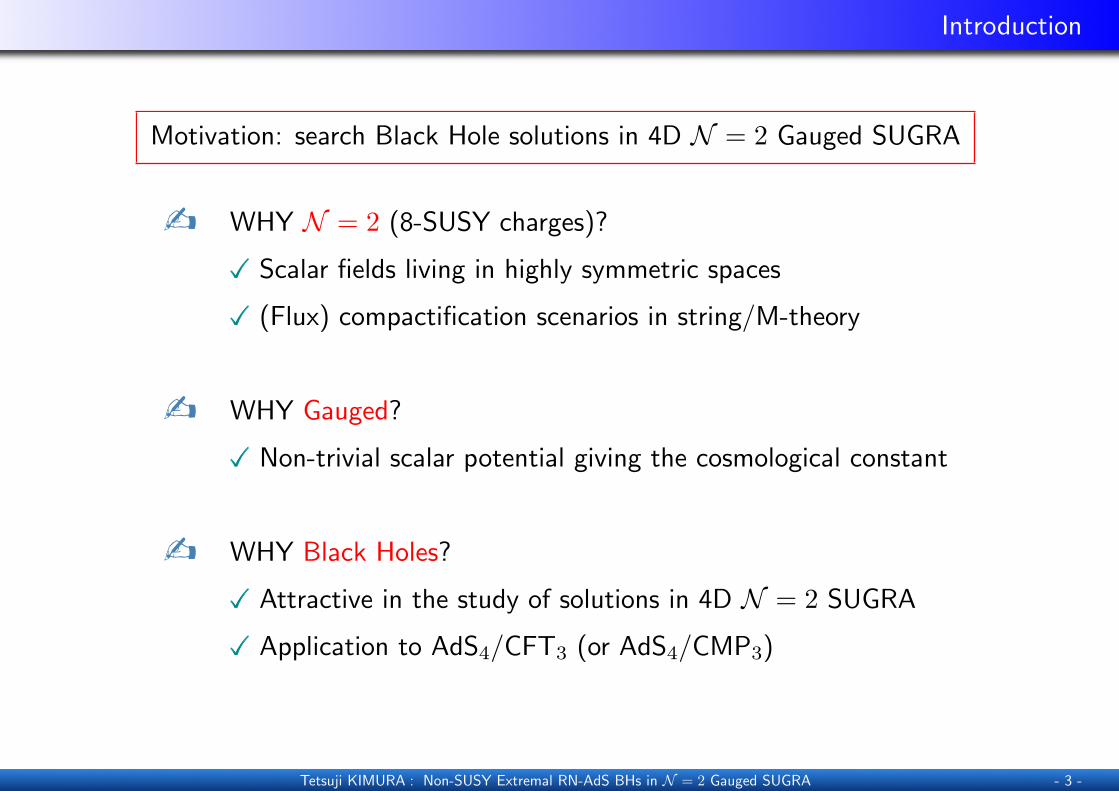
Motivation: search Black Hole solutions in 4D N = 2 Gauged SUGRA
b WHY N = 2 (8-SUSY charges)?
��� Scalar fields living in highly symmetric spaces
��� (Flux) compactification scenarios in string/M-theory
b WHY Gauged?
��� Non-trivial scalar potential giving the cosmological constant
b WHY Black Holes?
��� Attractive in the study of solutions in 4D N = 2 SUGRA
��� Application to AdS4/CFT3 (or AdS4/CMP3)
Tetsuji KIMURA : Non-SUSY Extremal RN-AdS BHs in N = 2 Gauged SUGRA - 3 -
Introduction
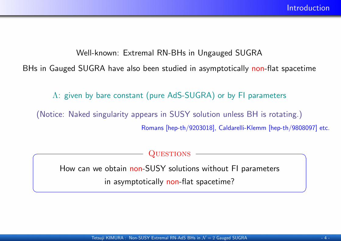
Well-known: Extremal RN-BHs in Ungauged SUGRA
BHs in Gauged SUGRA have also been studied in asymptotically non-flat spacetime
Λ: given by bare constant (pure AdS-SUGRA) or by FI parameters
(Notice: Naked singularity appears in SUSY solution unless BH is rotating.)
Romans [hep-th/9203018], Caldarelli-Klemm [hep-th/9808097] etc.
Questions� �How can we obtain non-SUSY solutions without FI parameters
in asymptotically non-flat spacetime?� �
Tetsuji KIMURA : Non-SUSY Extremal RN-AdS BHs in N = 2 Gauged SUGRA - 4 -
Contents
Introduction
N = 2 Gauged SUGRA
Effective Black Hole Potential
Attractor Equation
Single Modulus Model
Discussions
Contents
Introduction
N = 2 Gauged SUGRA
Effective Black Hole Potential
Attractor Equation
Single Modulus Model
Discussions
N = 2 Gauged SUGRA
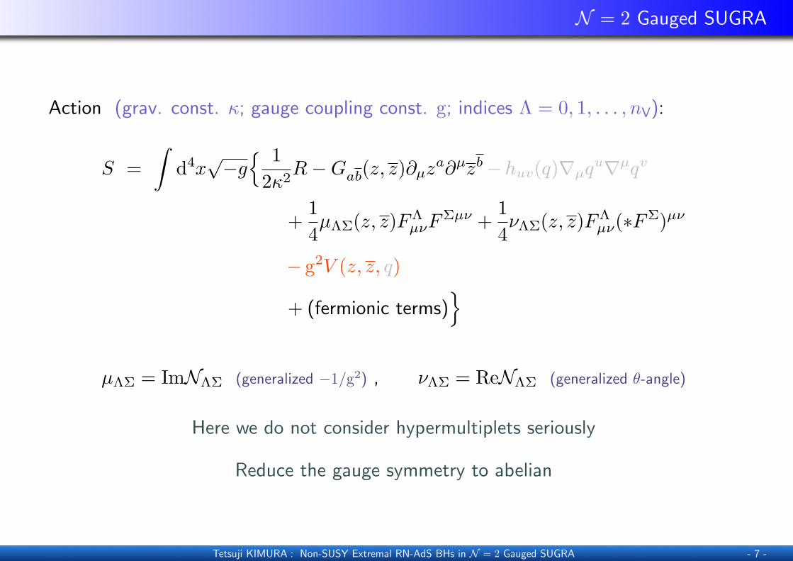
Action (grav. const. κ; gauge coupling const. g; indices Λ = 0, 1, . . . , nV):
S =∫
d4x√−g{ 1
2κ2R−Gab(z, z)∂µz
a∂µzb−huv(q)∇µqu∇µqv
+14µΛΣ(z, z)FΛ
µνFΣµν +
14νΛΣ(z, z)FΛ
µν(∗FΣ)µν
− g2V (z, z, q)
+ (fermionic terms)}
µΛΣ = ImNΛΣ (generalized −1/g2) , νΛΣ = ReNΛΣ (generalized θ-angle)
Here we do not consider hypermultiplets seriously
Reduce the gauge symmetry to abelian
Tetsuji KIMURA : Non-SUSY Extremal RN-AdS BHs in N = 2 Gauged SUGRA - 7 -
N = 2 Gauged SUGRA
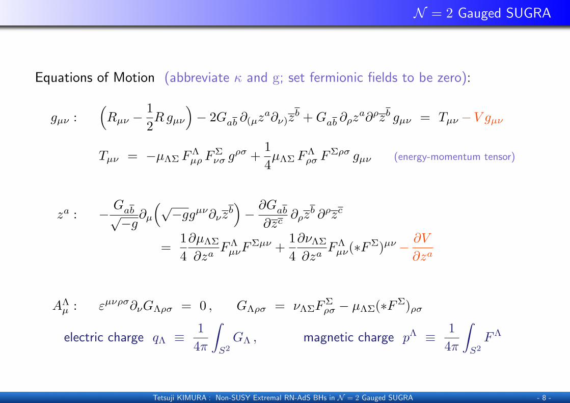
Equations of Motion (abbreviate κ and g; set fermionic fields to be zero):
gµν :(Rµν −
12Rgµν
)− 2Gab ∂(µz
a∂ν)zb +Gab ∂ρz
a∂ρzb gµν = Tµν −V gµν
Tµν = −µΛΣFΛµρF
Σνσ g
ρσ +14µΛΣF
Λρσ F
Σρσ gµν (energy-momentum tensor)
za : −Gab√−g
∂µ
(√−ggµν∂νz
b)−∂Gab
∂zc∂ρz
b ∂ρzc
=14∂µΛΣ
∂zaFΛ
µνFΣµν +
14∂νΛΣ
∂zaFΛ
µν(∗FΣ)µν − ∂V
∂za
AΛµ : εµνρσ∂νGΛρσ = 0 , GΛρσ = νΛΣF
Σρσ − µΛΣ(∗FΣ)ρσ
electric charge qΛ ≡14π
∫S2GΛ , magnetic charge pΛ ≡ 1
4π
∫S2FΛ
Tetsuji KIMURA : Non-SUSY Extremal RN-AdS BHs in N = 2 Gauged SUGRA - 8 -
Metric Ansatz
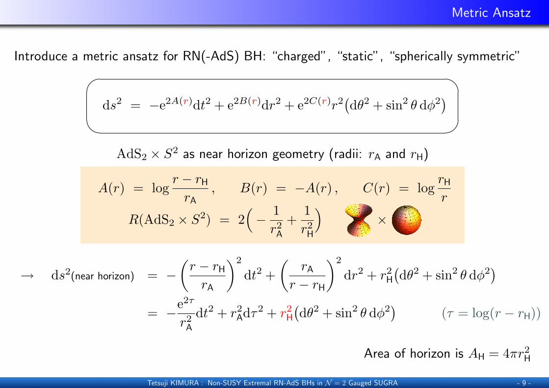
Introduce a metric ansatz for RN(-AdS) BH: “charged”, “static”, “spherically symmetric”
'
&
$
%ds2 = −e2A(r)dt2 + e2B(r)dr2 + e2C(r)r2
(dθ2 + sin2 θ dφ2
)AdS2 × S2 as near horizon geometry (radii: rA and rH)
A(r) = logr − rHrA
, B(r) = −A(r) , C(r) = logrHr
R(AdS2 × S2) = 2(− 1r2A
+1r2H
)×
→ ds2(near horizon) = −(r − rHrA
)2
dt2 +(
rAr − rH
)2
dr2 + r2H(dθ2 + sin2 θ dφ2
)= −e2τ
r2Adt2 + r2Adτ2 + r2H
(dθ2 + sin2 θ dφ2
)(τ = log(r − rH))
Area of horizon is AH = 4πr2H
Tetsuji KIMURA : Non-SUSY Extremal RN-AdS BHs in N = 2 Gauged SUGRA - 9 -
Metric Ansatz
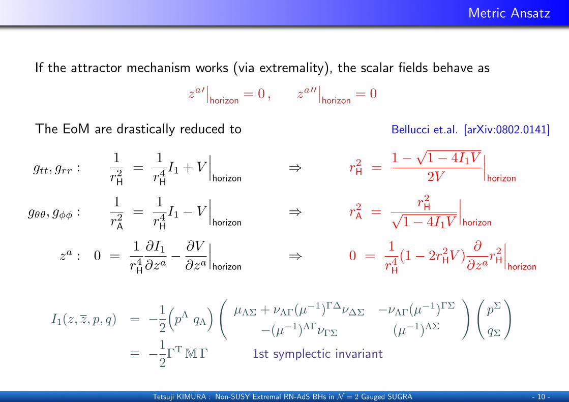
If the attractor mechanism works (via extremality), the scalar fields behave as
za′∣∣horizon
= 0 , za′′∣∣horizon
= 0
The EoM are drastically reduced to Bellucci et.al. [arXiv:0802.0141]
gtt, grr :1r2H
=1r4HI1 + V
∣∣∣horizon
⇒ r2H =1−√
1− 4I1V2V
∣∣∣horizon
gθθ, gφφ :1r2A
=1r4HI1 − V
∣∣∣horizon
⇒ r2A =r2H√
1− 4I1V
∣∣∣horizon
za : 0 =1r4H
∂I1∂za− ∂V
∂za
∣∣∣horizon
⇒ 0 =1r4H
(1− 2r2HV )∂
∂zar2H
∣∣∣horizon
I1(z, z, p, q) = −12
(pΛ qΛ
)( µΛΣ + νΛΓ(µ−1)Γ∆ν∆Σ −νΛΓ(µ−1)ΓΣ
−(µ−1)ΛΓνΓΣ (µ−1)ΛΣ
)(pΣ
qΣ
)≡ −1
2ΓT M Γ 1st symplectic invariant
Tetsuji KIMURA : Non-SUSY Extremal RN-AdS BHs in N = 2 Gauged SUGRA - 10 -
Effective Black Hole Potential
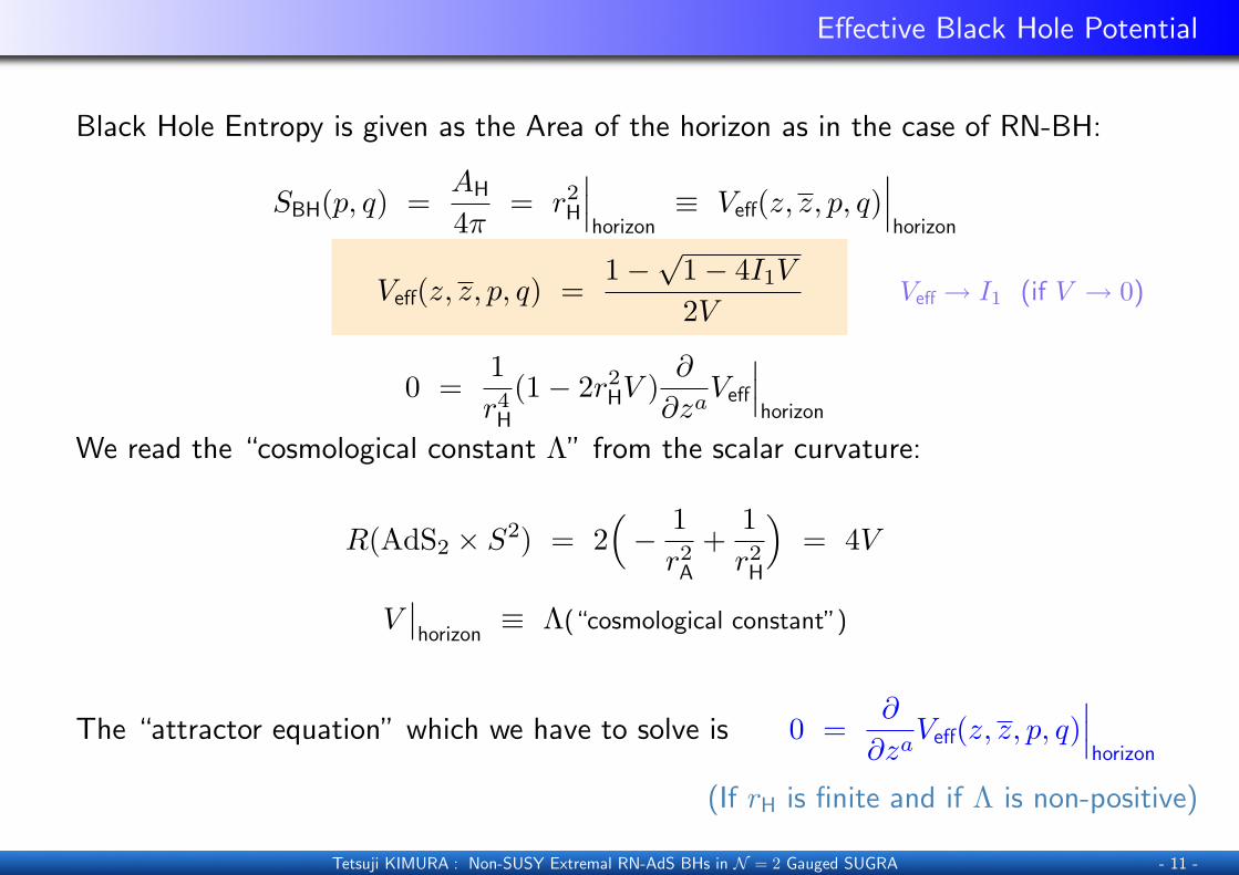
Black Hole Entropy is given as the Area of the horizon as in the case of RN-BH:
SBH(p, q) =AH
4π= r2H
∣∣∣horizon
≡ Veff(z, z, p, q)∣∣∣horizon
Veff(z, z, p, q) =1−√
1− 4I1V2V
Veff → I1 (if V → 0)
0 =1r4H
(1− 2r2HV )∂
∂zaVeff
∣∣∣horizon
We read the “cosmological constant Λ” from the scalar curvature:
R(AdS2 × S2) = 2(− 1r2A
+1r2H
)= 4V
V∣∣horizon
≡ Λ(“cosmological constant”)
The “attractor equation” which we have to solve is 0 =∂
∂zaVeff(z, z, p, q)
∣∣∣horizon
(If rH is finite and if Λ is non-positive)
Tetsuji KIMURA : Non-SUSY Extremal RN-AdS BHs in N = 2 Gauged SUGRA - 11 -
Effective Black Hole Potential
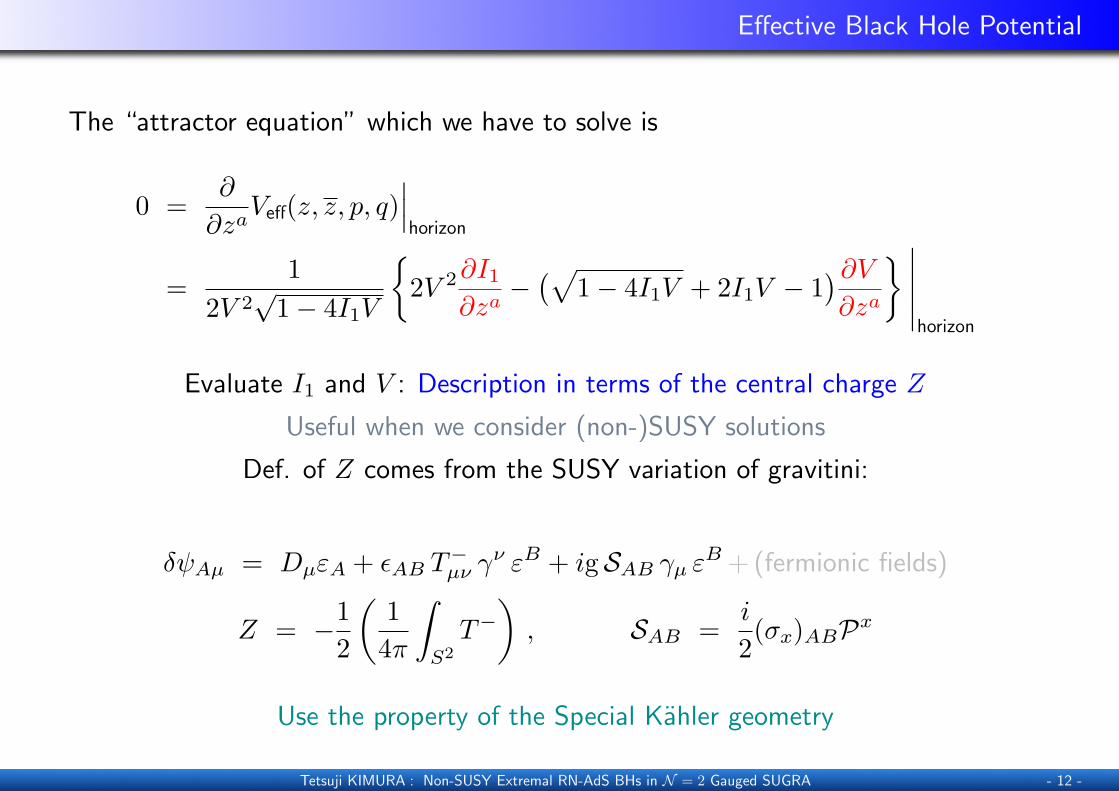
The “attractor equation” which we have to solve is
0 =∂
∂zaVeff(z, z, p, q)
∣∣∣horizon
=1
2V 2√
1− 4I1V
{2V 2∂I1
∂za−(√
1− 4I1V + 2I1V − 1)∂V∂za
} ∣∣∣∣∣horizon
Evaluate I1 and V : Description in terms of the central charge Z
Useful when we consider (non-)SUSY solutions
Def. of Z comes from the SUSY variation of gravitini:
δψAµ = DµεA + εAB T−µν γ
ν εB + igSAB γµ εB + (fermionic fields)
Z = −12
(14π
∫S2T−), SAB =
i
2(σx)ABPx
Use the property of the Special Kahler geometry
Tetsuji KIMURA : Non-SUSY Extremal RN-AdS BHs in N = 2 Gauged SUGRA - 12 -
Special Kahler Geometry
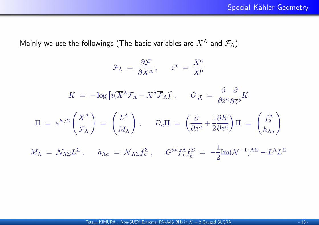
Mainly we use the followings (The basic variables are XΛ and FΛ):
FΛ =∂F∂XΛ
, za =Xa
X0
K = − log[i(XΛFΛ −XΛFΛ)
], Gab =
∂
∂za
∂
∂zbK
Π = eK/2
(XΛ
FΛ
)=
(LΛ
MΛ
), DaΠ =
(∂
∂za+
12∂K
∂za
)Π =
(fΛ
a
hΛa
)
MΛ = NΛΣLΣ , hΛa = NΛΣf
Σa , GabfΛ
a fΣb
= −12Im(N−1)ΛΣ − LΛLΣ
Tetsuji KIMURA : Non-SUSY Extremal RN-AdS BHs in N = 2 Gauged SUGRA - 13 -
Special Kahler Geometry
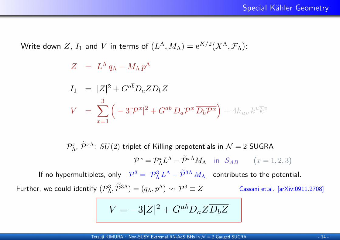
Write down Z, I1 and V in terms of (LΛ,MΛ) = eK/2(XΛ,FΛ):
Z = LΛ qΛ −MΛ pΛ
I1 = |Z|2 +GabDaZDbZ
V =3∑
x=1
(− 3|Px|2 +GabDaPxDbPx
)+ 4huv k
ukv
PxΛ, PxΛ: SU(2) triplet of Killing prepotentials in N = 2 SUGRA
Px = PxΛL
Λ − PxΛMΛ in SAB (x = 1, 2, 3)
If no hypermultiplets, only P3 = P3ΛL
Λ − P3ΛMΛ contributes to the potential.
Further, we could identify (P3Λ, P3Λ) = (qΛ, pΛ) P3 ≡ Z Cassani et.al. [arXiv:0911.2708]
V = −3|Z|2 +GabDaZDbZ
Tetsuji KIMURA : Non-SUSY Extremal RN-AdS BHs in N = 2 Gauged SUGRA - 14 -
Attractor Equation
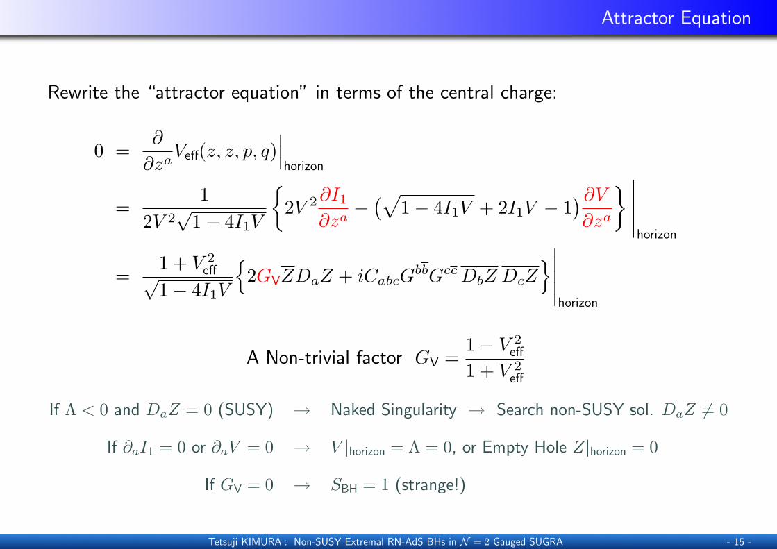
Rewrite the “attractor equation” in terms of the central charge:
0 =∂
∂zaVeff(z, z, p, q)
∣∣∣horizon
=1
2V 2√
1− 4I1V
{2V 2∂I1
∂za−(√
1− 4I1V + 2I1V − 1)∂V∂za
} ∣∣∣∣∣horizon
=1 + V 2
eff√1− 4I1V
{2GVZDaZ + iCabcG
bbGccDbZ DcZ}∣∣∣∣∣
horizon
A Non-trivial factor GV =1− V 2
eff
1 + V 2eff
If Λ < 0 and DaZ = 0 (SUSY) → Naked Singularity → Search non-SUSY sol. DaZ 6= 0
If ∂aI1 = 0 or ∂aV = 0 → V |horizon = Λ = 0, or Empty Hole Z|horizon = 0
If GV = 0 → SBH = 1 (strange!)
Tetsuji KIMURA : Non-SUSY Extremal RN-AdS BHs in N = 2 Gauged SUGRA - 15 -
Attractor Equation
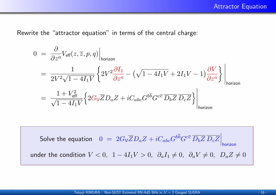
Rewrite the “attractor equation” in terms of the central charge:
0 =∂
∂zaVeff(z, z, p, q)
∣∣∣horizon
=1
2V 2√
1− 4I1V
{2V 2∂I1
∂za−(√
1− 4I1V + 2I1V − 1)∂V∂za
} ∣∣∣∣∣horizon
=1 + V 2
eff√1− 4I1V
{2GVZDaZ + iCabcG
bbGccDbZ DcZ}∣∣∣∣∣
horizon
Solve the equation 0 = 2GVZDaZ + iCabcGbbGccDbZ DcZ
∣∣∣horizon
under the condition V < 0, 1− 4I1V > 0, ∂aI1 6= 0, ∂aV 6= 0, DaZ 6= 0
Tetsuji KIMURA : Non-SUSY Extremal RN-AdS BHs in N = 2 Gauged SUGRA - 16 -
Contents
Introduction
N = 2 Gauged SUGRA
Effective Black Hole Potential
Attractor Equation
Single Modulus Model
Discussions
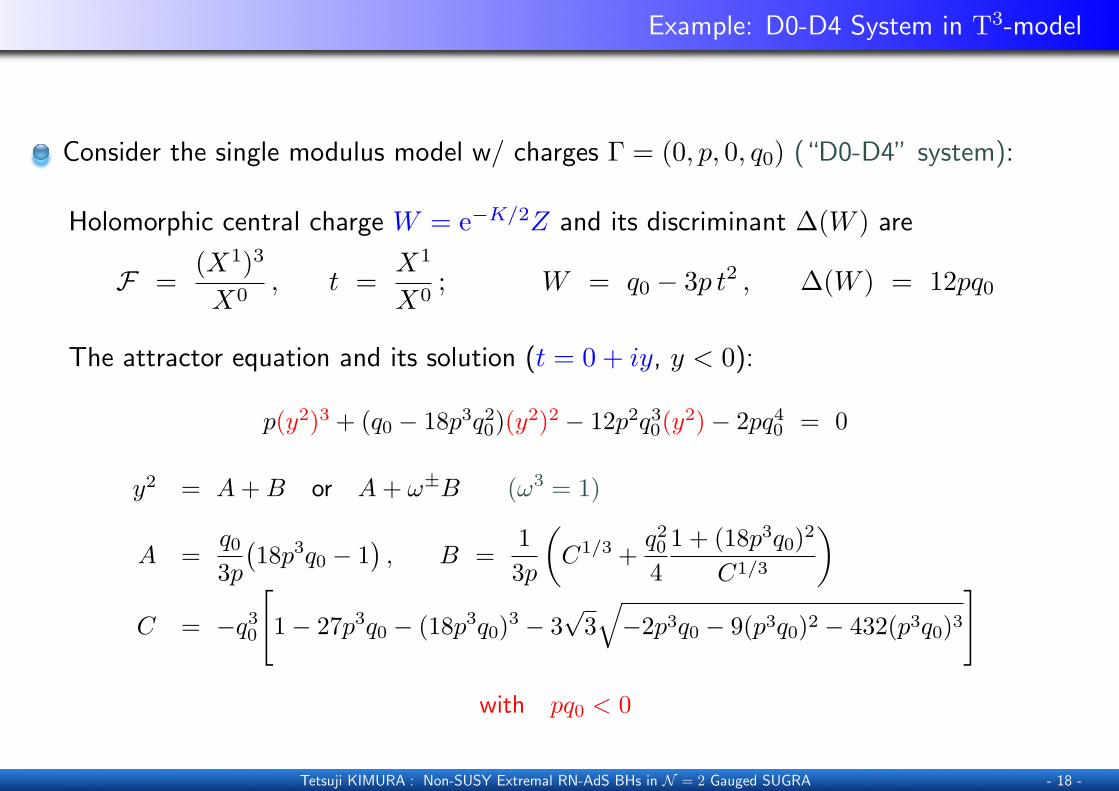
Example: D0-D4 System in T3-model
Consider the single modulus model w/ charges Γ = (0, p, 0, q0) (“D0-D4” system):
Holomorphic central charge W = e−K/2Z and its discriminant ∆(W ) are
F =(X1)3
X0, t =
X1
X0; W = q0 − 3p t2 , ∆(W ) = 12pq0
The attractor equation and its solution (t = 0 + iy, y < 0):
p(y2)3 + (q0 − 18p3q20)(y2)2 − 12p2q30(y
2)− 2pq40 = 0
y2 = A+B or A+ ω±B (ω3 = 1)
A =q03p(18p3q0 − 1
), B =
13p
(C1/3 +
q204
1 + (18p3q0)2
C1/3
)C = −q30
[1− 27p3q0 − (18p3q0)3 − 3
√3√−2p3q0 − 9(p3q0)2 − 432(p3q0)3
]
with pq0 < 0
Tetsuji KIMURA : Non-SUSY Extremal RN-AdS BHs in N = 2 Gauged SUGRA - 18 -
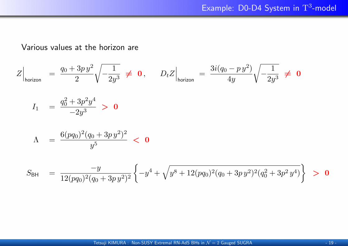
Example: D0-D4 System in T3-model
Various values at the horizon are
Z∣∣∣horizon
=q0 + 3p y2
2
√− 1
2y36= 0 , DtZ
∣∣∣horizon
=3i(q0 − p y2)
4y
√− 1
2y36= 0
I1 =q20 + 3p2y4
−2y3> 0
Λ =6(pq0)2(q0 + 3p y2)2
y5< 0
SBH =−y
12(pq0)2(q0 + 3p y2)2
{−y4 +
√y8 + 12(pq0)2(q0 + 3p y2)2(q20 + 3p2 y4)
}> 0
Tetsuji KIMURA : Non-SUSY Extremal RN-AdS BHs in N = 2 Gauged SUGRA - 19 -
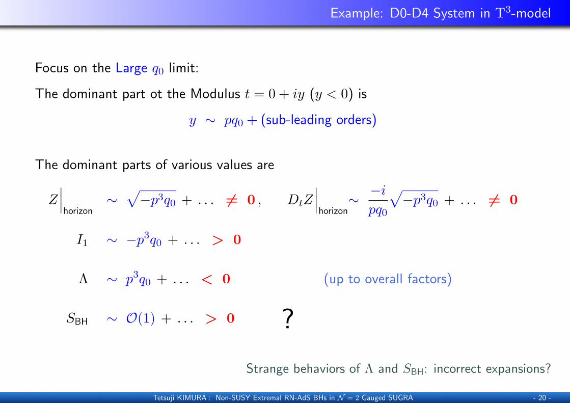
Example: D0-D4 System in T3-model
Focus on the Large q0 limit:
The dominant part ot the Modulus t = 0 + iy (y < 0) is
y ∼ pq0 + (sub-leading orders)
The dominant parts of various values are
Z∣∣∣horizon
∼√−p3q0 + . . . 6= 0 , DtZ
∣∣∣horizon
∼ −ipq0
√−p3q0 + . . . 6= 0
I1 ∼ −p3q0 + . . . > 0
Λ ∼ p3q0 + . . . < 0 (up to overall factors)
SBH ∼ O(1) + . . . > 0 ?
Strange behaviors of Λ and SBH: incorrect expansions?
Tetsuji KIMURA : Non-SUSY Extremal RN-AdS BHs in N = 2 Gauged SUGRA - 20 -
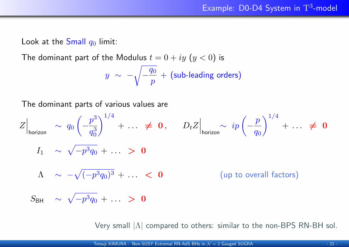
Example: D0-D4 System in T3-model
Look at the Small q0 limit:
The dominant part of the Modulus t = 0 + iy (y < 0) is
y ∼ −√−q0p
+ (sub-leading orders)
The dominant parts of various values are
Z∣∣∣horizon
∼ q0
(−p
3
q30
)1/4
+ . . . 6= 0 , DtZ∣∣∣horizon
∼ ip
(− pq0
)1/4
+ . . . 6= 0
I1 ∼√−p3q0 + . . . > 0
Λ ∼ −√
(−p3q0)3 + . . . < 0 (up to overall factors)
SBH ∼√−p3q0 + . . . > 0
Very small |Λ| compared to others: similar to the non-BPS RN-BH sol.
Tetsuji KIMURA : Non-SUSY Extremal RN-AdS BHs in N = 2 Gauged SUGRA - 21 -
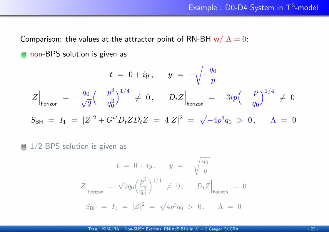
Example’: D0-D4 System in T3-model
Comparison: the values at the attractor point of RN-BH w/ Λ = 0:
non-BPS solution is given as
t = 0 + iy , y = −√−q0p
Z∣∣∣horizon
= − q0√2
(− p
3
q30
)1/4
6= 0 , DtZ∣∣∣horizon
= −3ip(− p
q0
)1/4
6= 0
SBH = I1 = |Z|2 +GttDtZDtZ = 4|Z|2 =√−4p3q0 > 0 , Λ = 0
1/2-BPS solution is given as
t = 0 + iy , y = −√q0p
Z∣∣∣horizon
=√
2q0( p3
q30
)1/4
6= 0 , DtZ∣∣∣horizon
= 0
SBH = I1 = |Z|2 =√
4p3q0 > 0 , Λ = 0
Tetsuji KIMURA : Non-SUSY Extremal RN-AdS BHs in N = 2 Gauged SUGRA - 22 -
Contents
Introduction
N = 2 Gauged SUGRA
Effective Black Hole Potential
Attractor Equation
Single Modulus Model
Discussions
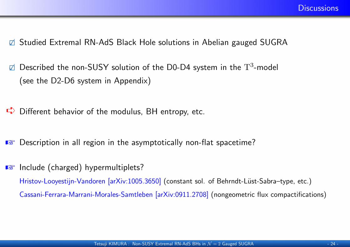
Discussions
2� Studied Extremal RN-AdS Black Hole solutions in Abelian gauged SUGRA
2� Described the non-SUSY solution of the D0-D4 system in the T3-model
(see the D2-D6 system in Appendix)
ê Different behavior of the modulus, BH entropy, etc.
Z Description in all region in the asymptotically non-flat spacetime?
Z Include (charged) hypermultiplets?
Hristov-Looyestijn-Vandoren [arXiv:1005.3650] (constant sol. of Behrndt-Lust-Sabra–type, etc.)
Cassani-Ferrara-Marrani-Morales-Samtleben [arXiv:0911.2708] (nongeometric flux compactifications)
Tetsuji KIMURA : Non-SUSY Extremal RN-AdS BHs in N = 2 Gauged SUGRA - 24 -

Fin

Appendix
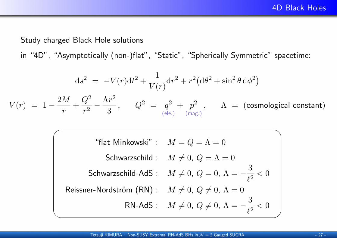
4D Black Holes
Study charged Black Hole solutions
in “4D”, “Asymptotically (non-)flat”, “Static”, “Spherically Symmetric” spacetime:
ds2 = −V (r)dt2 +1
V (r)dr2 + r2
(dθ2 + sin2 θ dφ2
)V (r) = 1− 2M
r+Q2
r2− Λr2
3, Q2 = q2
(ele.)
+ p2
(mag.)
, Λ = (cosmological constant)
'
&
$
%
“flat Minkowski” : M = Q = Λ = 0
Schwarzschild : M 6= 0, Q = Λ = 0
Schwarzschild-AdS : M 6= 0, Q = 0, Λ = − 3`2< 0
Reissner-Nordstrom (RN) : M 6= 0, Q 6= 0, Λ = 0
RN-AdS : M 6= 0, Q 6= 0, Λ = − 3`2< 0
Tetsuji KIMURA : Non-SUSY Extremal RN-AdS BHs in N = 2 Gauged SUGRA - 27 -
N = 2 Gauged SUGRA
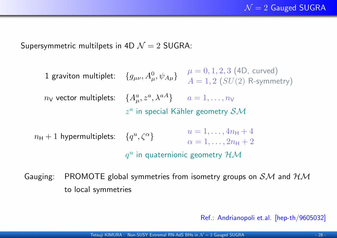
Supersymmetric multilpets in 4D N = 2 SUGRA:
1 graviton multiplet: {gµν, A0µ, ψAµ}
µ = 0, 1, 2, 3 (4D, curved)A = 1, 2 (SU(2) R-symmetry)
nV vector multiplets: {Aaµ, z
a, λaA} a = 1, . . . , nV
za in special Kahler geometry SM
nH + 1 hypermultiplets: {qu, ζα} u = 1, . . . , 4nH + 4α = 1, . . . , 2nH + 2
qu in quaternionic geometry HM
Gauging: PROMOTE global symmetries from isometry groups on SM and HMto local symmetries
Ref.: Andrianopoli et.al. [hep-th/9605032]
Tetsuji KIMURA : Non-SUSY Extremal RN-AdS BHs in N = 2 Gauged SUGRA - 28 -

Identity
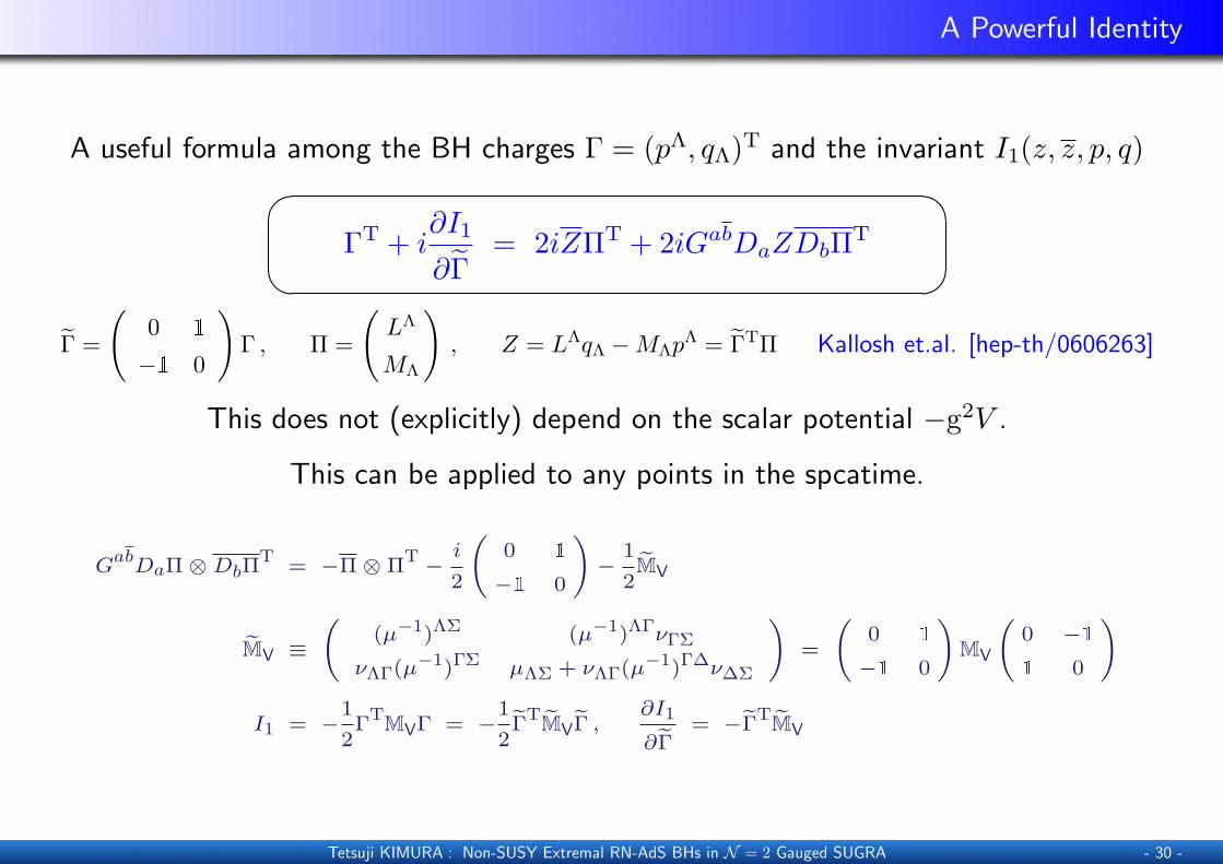
A Powerful Identity
A useful formula among the BH charges Γ = (pΛ, qΛ)T and the invariant I1(z, z, p, q)�
�
�
�ΓT + i
∂I1
∂Γ= 2iZΠT + 2iGabDaZDbΠT
Γ =
(0 1
−1 0
)Γ , Π =
(LΛ
MΛ
), Z = LΛqΛ −MΛp
Λ = ΓTΠ Kallosh et.al. [hep-th/0606263]
This does not (explicitly) depend on the scalar potential −g2V .
This can be applied to any points in the spcatime.
Gab
DaΠ ⊗ DbΠT
= −Π ⊗ ΠT −
i
2
0 1
−1 0
!
−1
2eMV
eMV ≡
(µ−1)ΛΣ (µ−1)ΛΓνΓΣ
νΛΓ(µ−1)ΓΣ µΛΣ + νΛΓ(µ−1)Γ∆ν∆Σ
!
=
0 1
−1 0
!
MV
0 −1
1 0
!
I1 = −1
2Γ
TMVΓ = −1
2eΓ
TeMVeΓ ,
∂I1
∂eΓ= −eΓT
eMV
Tetsuji KIMURA : Non-SUSY Extremal RN-AdS BHs in N = 2 Gauged SUGRA - 30 -
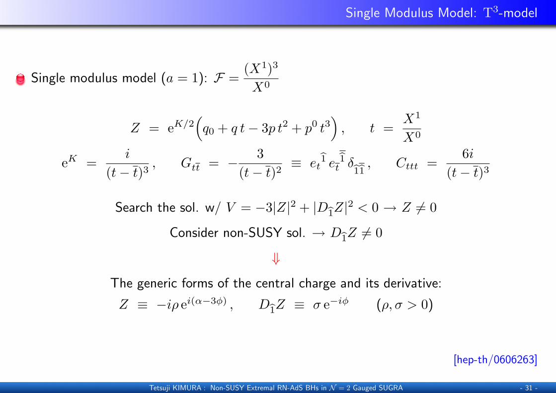
Single Modulus Model: T3-model
Single modulus model (a = 1): F =(X1)3
X0
Z = eK/2(q0 + q t− 3p t2 + p0 t3
), t =
X1
X0
eK =i
(t− t)3, Gtt = − 3
(t− t)2≡ et
b1 etb1 δb1b1, Cttt =
6i(t− t)3
Search the sol. w/ V = −3|Z|2 + |Db1Z|2 < 0 → Z 6= 0
Consider non-SUSY sol. → Db1Z 6= 0
⇓
The generic forms of the central charge and its derivative:
Z ≡ −iρ ei(α−3φ) , Db1Z ≡ σ e−iφ (ρ, σ > 0)
[hep-th/0606263]
Tetsuji KIMURA : Non-SUSY Extremal RN-AdS BHs in N = 2 Gauged SUGRA - 31 -
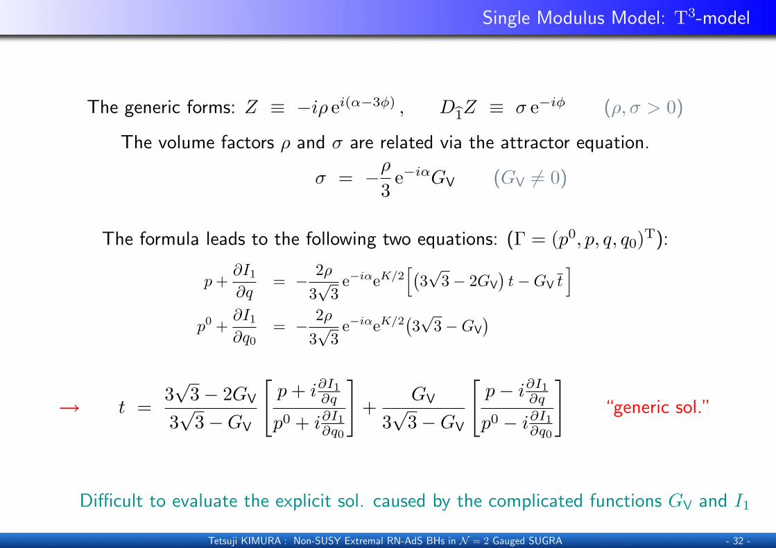
Single Modulus Model: T3-model
The generic forms: Z ≡ −iρ ei(α−3φ) , Db1Z ≡ σ e−iφ (ρ, σ > 0)
The volume factors ρ and σ are related via the attractor equation.
σ = −ρ3
e−iαGV (GV 6= 0)
The formula leads to the following two equations: (Γ = (p0, p, q, q0)T):
p+∂I1∂q
= − 2ρ3√
3e−iαeK/2
[(3√
3− 2GV
)t−GV t
]p0 +
∂I1∂q0
= − 2ρ3√
3e−iαeK/2
(3√
3−GV
)
→ t =3√
3− 2GV
3√
3−GV
[p+ i∂I1
∂q
p0 + i∂I1∂q0
]+
GV
3√
3−GV
[p− i∂I1
∂q
p0 − i∂I1∂q0
]“generic sol.”
Difficult to evaluate the explicit sol. caused by the complicated functions GV and I1
Tetsuji KIMURA : Non-SUSY Extremal RN-AdS BHs in N = 2 Gauged SUGRA - 32 -
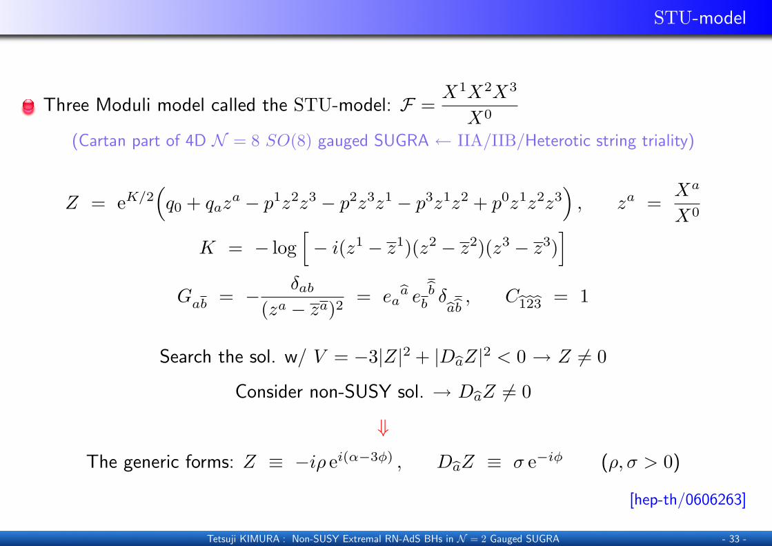
STU-model
Three Moduli model called the STU-model: F =X1X2X3
X0
(Cartan part of 4D N = 8 SO(8) gauged SUGRA ← IIA/IIB/Heterotic string triality)
Z = eK/2(q0 + qaz
a − p1z2z3 − p2z3z1 − p3z1z2 + p0z1z2z3), za =
Xa
X0
K = − log[− i(z1 − z1)(z2 − z2)(z3 − z3)
]Gab = − δab
(za − za)2= ea
ba eb
bb δbabb, C
b1b2b3 = 1
Search the sol. w/ V = −3|Z|2 + |DbaZ|2 < 0 → Z 6= 0
Consider non-SUSY sol. → DbaZ 6= 0
⇓
The generic forms: Z ≡ −iρ ei(α−3φ) , DbaZ ≡ σ e−iφ (ρ, σ > 0)
[hep-th/0606263]
Tetsuji KIMURA : Non-SUSY Extremal RN-AdS BHs in N = 2 Gauged SUGRA - 33 -
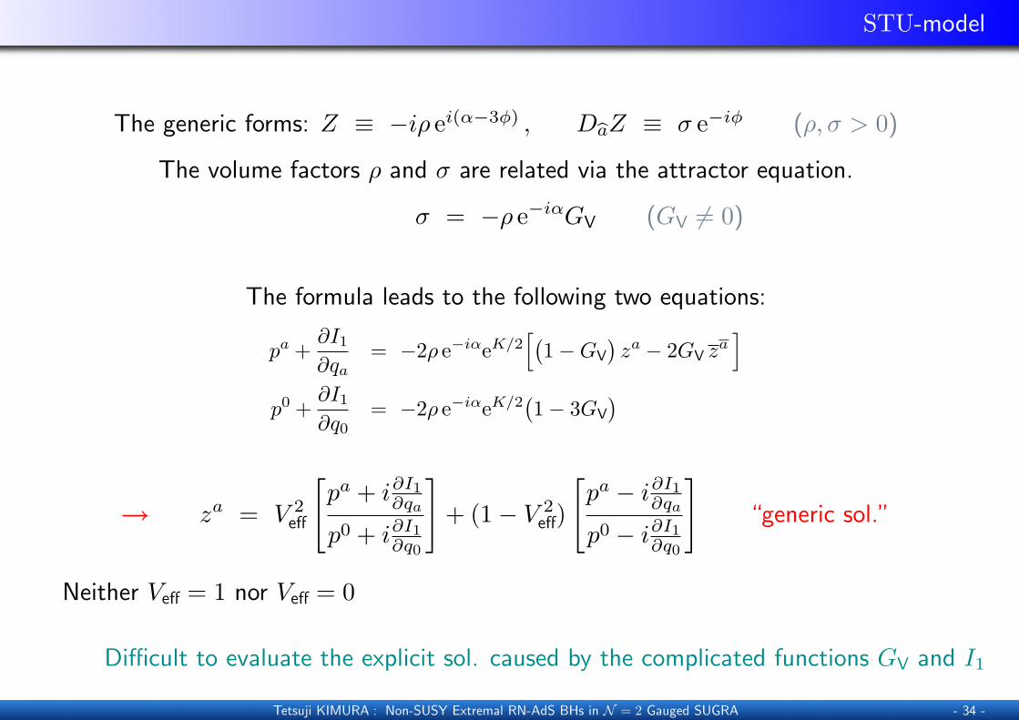
STU-model
The generic forms: Z ≡ −iρ ei(α−3φ) , DbaZ ≡ σ e−iφ (ρ, σ > 0)
The volume factors ρ and σ are related via the attractor equation.
σ = −ρ e−iαGV (GV 6= 0)
The formula leads to the following two equations:
pa +∂I1∂qa
= −2ρ e−iαeK/2[(
1−GV
)za − 2GV z
a]
p0 +∂I1∂q0
= −2ρ e−iαeK/2(1− 3GV
)
→ za = V 2eff
[pa + i∂I1
∂qa
p0 + i∂I1∂q0
]+ (1− V 2
eff)
[pa − i∂I1
∂qa
p0 − i∂I1∂q0
]“generic sol.”
Neither Veff = 1 nor Veff = 0
Difficult to evaluate the explicit sol. caused by the complicated functions GV and I1
Tetsuji KIMURA : Non-SUSY Extremal RN-AdS BHs in N = 2 Gauged SUGRA - 34 -
Another Example in T3-model
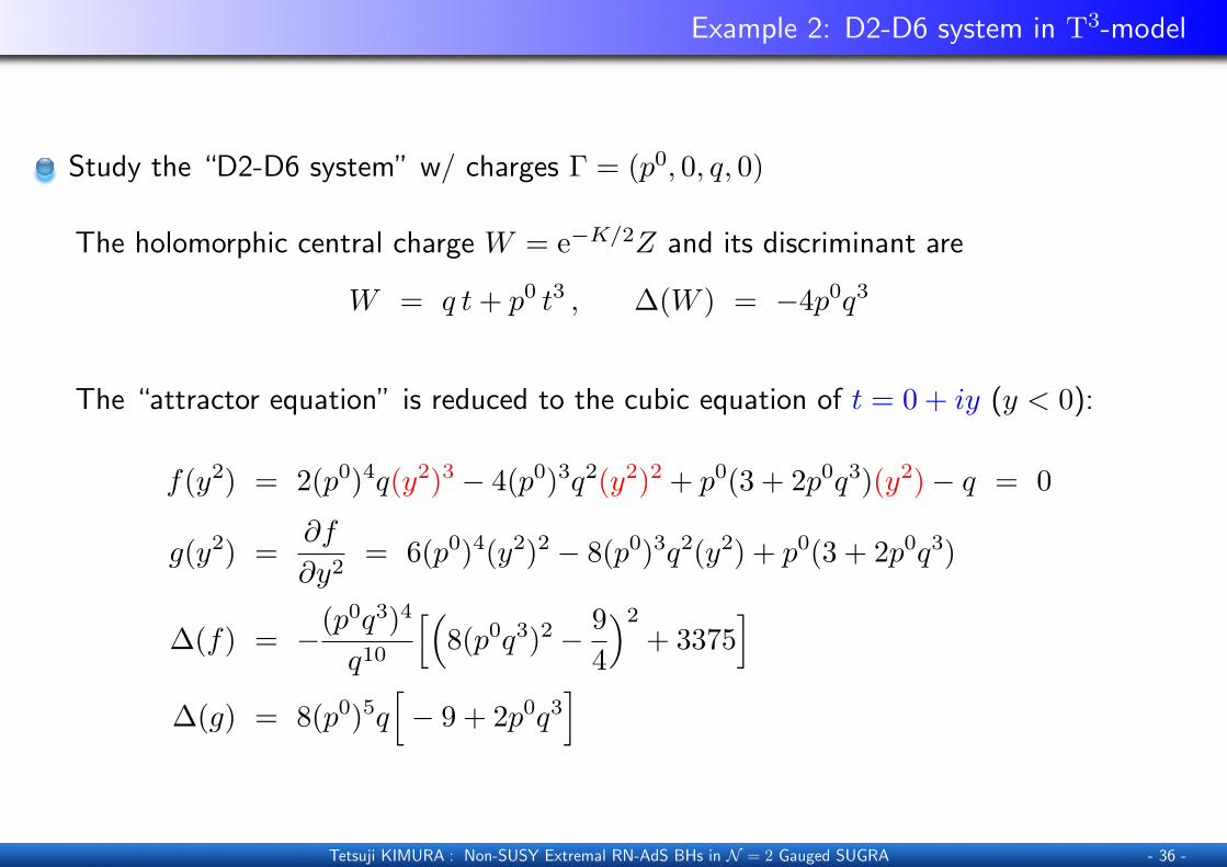
Example 2: D2-D6 system in T3-model
Study the “D2-D6 system” w/ charges Γ = (p0, 0, q, 0)
The holomorphic central charge W = e−K/2Z and its discriminant are
W = q t+ p0 t3 , ∆(W ) = −4p0q3
The “attractor equation” is reduced to the cubic equation of t = 0 + iy (y < 0):
f(y2) = 2(p0)4q(y2)3 − 4(p0)3q2(y2)2 + p0(3 + 2p0q3)(y2)− q = 0
g(y2) =∂f
∂y2= 6(p0)4(y2)2 − 8(p0)3q2(y2) + p0(3 + 2p0q3)
∆(f) = −(p0q3)4
q10
[(8(p0q3)2 − 9
4
)2
+ 3375]
∆(g) = 8(p0)5q[− 9 + 2p0q3
]
Tetsuji KIMURA : Non-SUSY Extremal RN-AdS BHs in N = 2 Gauged SUGRA - 36 -
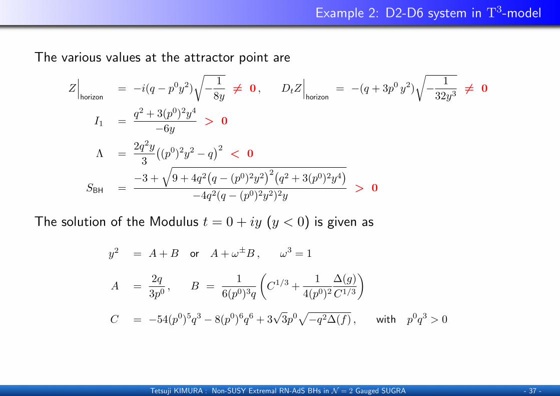
Example 2: D2-D6 system in T3-model
The various values at the attractor point are
Z∣∣∣horizon
= −i(q − p0y2)√− 1
8y6= 0 , DtZ
∣∣∣horizon
= −(q + 3p0 y2)√− 1
32y36= 0
I1 =q2 + 3(p0)2y4
−6y> 0
Λ =2q2y
3((p0)2y2 − q
)2< 0
SBH =−3 +
√9 + 4q2
(q − (p0)2y2
)2(q2 + 3(p0)2y4
)−4q2(q − (p0)2y2)2y
> 0
The solution of the Modulus t = 0 + iy (y < 0) is given as
y2 = A+B or A+ ω±B , ω3 = 1
A =2q3p0
, B =1
6(p0)3q
(C1/3 +
14(p0)2
∆(g)C1/3
)C = −54(p0)5q3 − 8(p0)6q6 + 3
√3p0√−q2∆(f) , with p0q3 > 0
Tetsuji KIMURA : Non-SUSY Extremal RN-AdS BHs in N = 2 Gauged SUGRA - 37 -
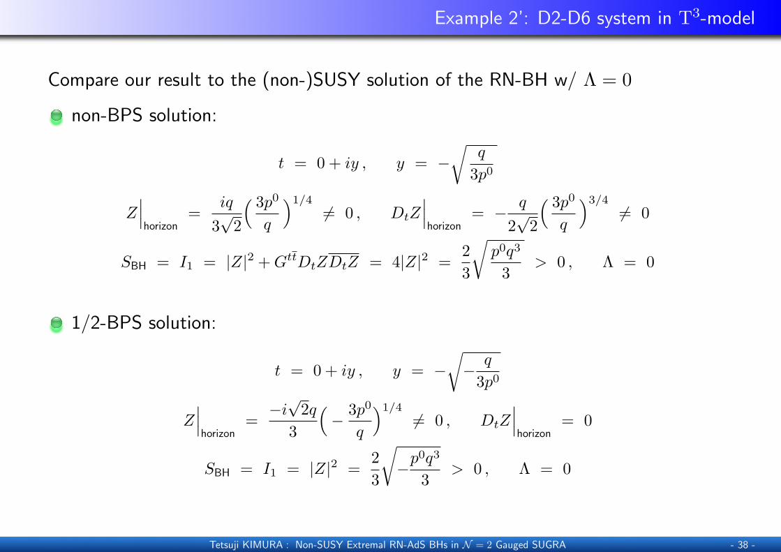
Example 2’: D2-D6 system in T3-model
Compare our result to the (non-)SUSY solution of the RN-BH w/ Λ = 0
non-BPS solution:
t = 0 + iy , y = −√
q
3p0
Z∣∣∣horizon
=iq
3√
2
( 3p0
q
)1/4
6= 0 , DtZ∣∣∣horizon
= − q
2√
2
( 3p0
q
)3/4
6= 0
SBH = I1 = |Z|2 +GttDtZDtZ = 4|Z|2 =23
√p0q3
3> 0 , Λ = 0
1/2-BPS solution:
t = 0 + iy , y = −√− q
3p0
Z∣∣∣horizon
=−i√
2q3
(− 3p0
q
)1/4
6= 0 , DtZ∣∣∣horizon
= 0
SBH = I1 = |Z|2 =23
√−p
0q3
3> 0 , Λ = 0
Tetsuji KIMURA : Non-SUSY Extremal RN-AdS BHs in N = 2 Gauged SUGRA - 38 -

Hypermultiplets
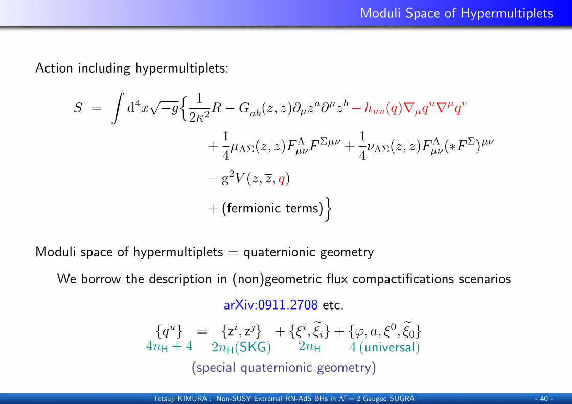
Moduli Space of Hypermultiplets
Action including hypermultiplets:
S =∫
d4x√−g{ 1
2κ2R−Gab(z, z)∂µz
a∂µzb−huv(q)∇µqu∇µqv
+14µΛΣ(z, z)FΛ
µνFΣµν +
14νΛΣ(z, z)FΛ
µν(∗FΣ)µν
− g2V (z, z, q)
+ (fermionic terms)}
Moduli space of hypermultiplets = quaternionic geometry
We borrow the description in (non)geometric flux compactifications scenarios
arXiv:0911.2708 etc.
{qu}4nH + 4
= {zi, z}2nH(SKG)
+ {ξi, ξi}2nH
+ {ϕ, a, ξ0, ξ0}4 (universal)
(special quaternionic geometry)
Tetsuji KIMURA : Non-SUSY Extremal RN-AdS BHs in N = 2 Gauged SUGRA - 40 -
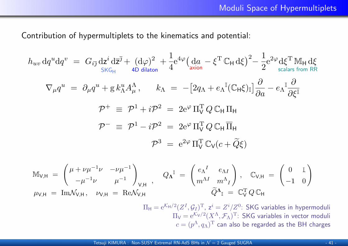
Moduli Space of Hypermultiplets
Contribution of hypermultiplets to the kinematics and potential:
huv dqudqv = Gi dzi dz +SKGH
(dϕ)24D dilaton
+14e4ϕ(
daaxion− ξT CH dξ
)2− 12e2ϕdξT MH dξ
scalars from RR
∇µqu = ∂µq
u + g kuΛA
Λµ , kΛ = −
[2qΛ + eΛ
I(CHξ)I] ∂∂a− eΛI ∂
∂ξI
P+ ≡ P1 + iP2 = 2eϕ ΠTV QCH ΠH
P− ≡ P1 − iP2 = 2eϕ ΠTV QCH ΠH
P3 = e2ϕ ΠTV CV(c+ Qξ)
MV,H =
(µ+ νµ−1ν −νµ−1
−µ−1ν µ−1
)V,H
µV,H = ImNV,H , νV,H = ReNV,H
,QΛ
I =
(eΛ
I eΛI
mΛI mΛI
), CV,H =
(0 1
−1 0
)QΛ
I = CTV QCH
ΠH = eKH/2(ZI,GI)T, zi = Zi/Z0: SKG variables in hypermoduli
ΠV = eKV/2(XΛ,FΛ)T: SKG variables in vector modulic = (pΛ, qΛ)T can also be regarded as the BH charges
Tetsuji KIMURA : Non-SUSY Extremal RN-AdS BHs in N = 2 Gauged SUGRA - 41 -
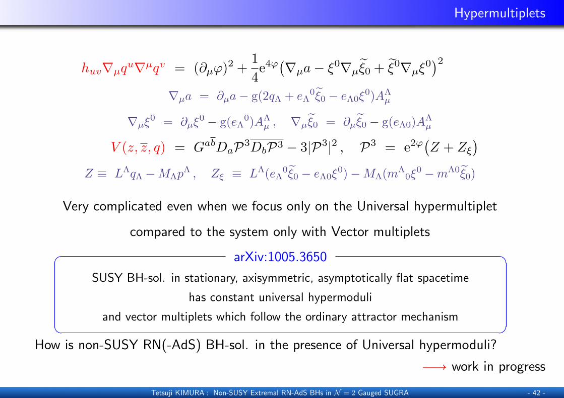
Hypermultiplets
huv∇µqu∇µqv = (∂µϕ)2 +
14e4ϕ(∇µa− ξ0∇µξ0 + ξ0∇µξ
0)2
∇µa = ∂µa− g(2qΛ + eΛ0ξ0 − eΛ0ξ
0)AΛµ
∇µξ0 = ∂µξ
0 − g(eΛ0)AΛµ , ∇µξ0 = ∂µξ0 − g(eΛ0)AΛ
µ
V (z, z, q) = GabDaP3DbP3 − 3|P3|2 , P3 = e2ϕ(Z + Zξ
)Z ≡ LΛqΛ −MΛp
Λ , Zξ ≡ LΛ(eΛ0ξ0 − eΛ0ξ0)−MΛ(mΛ
0ξ0 −mΛ0ξ0)
Very complicated even when we focus only on the Universal hypermultiplet
compared to the system only with Vector multiplets
arXiv:1005.3650� �SUSY BH-sol. in stationary, axisymmetric, asymptotically flat spacetime
has constant universal hypermoduli
and vector multiplets which follow the ordinary attractor mechanism� �How is non-SUSY RN(-AdS) BH-sol. in the presence of Universal hypermoduli?
−→ work in progress
Tetsuji KIMURA : Non-SUSY Extremal RN-AdS BHs in N = 2 Gauged SUGRA - 42 -