Embed Size (px)
Citation preview
The extremal process of super-Brownian motion
Yan-Xia Ren∗ Renming Song† and Rui Zhang‡
Abstract
In this paper, we establish limit theorems for the supremum of the support, denotedby Mt, of a supercritical super-Brownian motion {Xt, t ≥ 0} on R. We prove that thereexists an m(t) such that (Xt −m(t),Mt −m(t)) converges in law, and give some largedeviation results for Mt as t → ∞. We also prove that the limit of the extremalprocess Et := Xt − m(t) is a Poisson random measure with exponential intensity inwhich each atom is decorated by an independent copy of an auxiliary measure. Theseresults are analogues of the results for branching Brownian motions obtained in Arguinet al. (Probab. Theory Relat. Fields 157 (2013), 535–574), Aıdekon et al. (Probab.Theory Relat. Fields 157 (2013), 405–451) and Roberts (Ann. Probab. 41 (2013),3518–3541).
AMS Subject Classifications (2010): Primary 60J68, 60F05; Secondary 60G57, 60G70
Keywords and Phrases: Super-Brownian motion, extremal process, supremum of thesupport of super-Brownian motion, Poisson random measure, KPP equation.
1 Introduction
1.1 Super-Brownian motion
Let ψ be a function of the form:
ψ(λ) = −αλ+ βλ2 +
∫ ∞0
(e−λy − 1 + λy
)n(dy), λ ≥ 0,
where α ∈ R, β ≥ 0 and n is a σ-finite measure satisfying∫ ∞0
(y2 ∧ y)n(dy) <∞.
∗The research of this author is supported by NSFC (Grant No. 11671017 and 11731009) and LMEQF.†Research supported in part by a grant from the Simons Foundation (#429343, Renming Song).‡The corresponding author. The research of this author is supported by NSFC (Grant No. 11601354),
Beijing Municipal Natural Science Foundation(Grant No. 1202004), and Academy for MultidisciplinaryStudies, Capital Normal University
1
ψ is called a branching mechanism. We will always assume that limλ→∞ ψ(λ) = ∞. Let
{Bt,Px} be a standard Brownian motion, and Ex be the corresponding expectation. In this
paper we will consider a super-Brownian motion X on R with branching mechanism ψ.
Let B+(R) (resp. B+b (R)) be the space of non-negative (resp. non-negative bounded)
Borel measurable function on R, and let MF (R) be the space of finite measures on R,
equipped with the topology of weak convergence. A super-Brownian motion X with branch-
ing mechanism ψ is a Markov process taking values in MF (R). The existence of such
superprocesses is well-known, see, for instance, [17], [18] or [30]. For any µ ∈ MF (R), we
denote the law of X with initial configuration µ by Pµ, and the corresponding expectation
by Eµ. As usual, we use the notation: 〈φ, µ〉 :=∫R φ(x)µ(dx) and ‖µ‖ := 〈1, µ〉. Then for
all φ ∈ B+b (R) and µ ∈MF (E),
− logEµ(e−〈φ,Xt〉
)= 〈uφ(t, ·), µ〉, (1.1)
where uφ(t, x) is the unique positive solution to the equation
uφ(t, x) + Ex
∫ t
0
ψ(uφ(t− s, Bs))ds = Exφ(Bt). (1.2)
Note that the integral equation (1.2) is equivalent to the equation:
∂
∂tuφ(t, x)− 1
2
∂2
∂x2uφ(t, x) = −ψ(uφ(t, x)), t > 0, x ∈ R, (1.3)
with initial condition uφ(0, x) = φ(x). Moreover, limt→0 uφ(t, x) = φ(x), if φ is a nonnegative
bounded continuous function on R.
X is called a supercritical (critical, subcritical) super Brownian motion if α > 0 (= 0, < 0).
In this paper, we only deal with the supercritical case, that is α > 0.
1.2 Maximal position of super-Brownian motion
The maximal positionMt of branching-Brownian motions has been studied intensively. With-
out loss of generality, we assume in this subsection that the branching rate is 1, and the
offspring distribution {pk} satisfies p0 = 0 and the mean of the offspring distribution is 2.
Denote by Pδ0 the law of branching Brownian motion starting from one point located at 0.
In the seminal paper [35], Kolmogorov, Petrovskii and Piskounov proved that Mt/t →√
2
in probability, which implies that the leading order of Mt is√
2t. In [8], Bramson provided
a log correction to the leading order of Mt. He proved in [8] (see also [9]) that, under some
moment conditions, Pδ0(Mt − m(t) ≤ x) → 1 − w(x) as t → ∞ for all x ∈ R, where
m(t) =√
2t − 32√
2log t and w(x) is a traveling wave solution. In [27], Lalley and Sellke
gave a probabilistic representation of the traveling wave solution in terms of the limit of the
derivative martingale of branching Brownian motion. In [42], Roberts gave another proof of
Bramson’s result and also an almost sure fluctuation result of Mt. Large deviation results
for Mt were obtained by Chauvin and Rouault in [15, 16].
2
Beyond the behavior of the maximal displacement of branching Brownian motions, the
full statistics of the extremal configurations was studied in Arguin et al. [3, 4, 5] and Aıdekon
et al. [2]. Assume the particles alive at time t are ordered decreasingly: xt1 ≥ xt2 ≥ · · · ≥ xtn(t),
where n(t) is the number of particles alive at time t. It is clear that xt1 is the maximum
position Mt at time t. Arguin et al. [4, 5] studied the limit property of the extremal process
of branching Brownian motion, which is the random measure defined by
Et :=
n(t)∑j=1
δxtj−m(t).
Note that Et = Yt − m(t), where Yt is the measure corresponding to configuration of the
positions of the particles alive at time t. In [5], using the results of [9], Arguin et al. first
proved that Et converges in law, which implies the weak convergence of xtk, the kth max-
imal displacement for each fixed integer k ≥ 1, and then gave a rigorous characterization
of the limiting extremal process. It was proved in [5] that the limiting process is a (ran-
domly shifted) Poisson cluster process, where the positions of the clusters form a Poisson
point process with an exponential intensity measure. The law of the individual clusters is
characterized as a branching Brownian motion conditioned to perform unusually large dis-
placements. Almost at the same time, Aıdekon et al. [2] proved similar results using a totally
different method.
In the recent paper [10], Berestycki et al. studied the asymptotic behavior of the extremal
particles of branching Ornstein-Uhlenbeck processes. For inhomogeneous branching Brown-
ian motions, many papers discussed the growth rate of the maximal position, see Bocharov
and Harris [12, 13] and Bocharov [11] for the case with catalytic branching at the origin,
Shiozawa [44], Nishimori et al. [39], Lalley and Sellke [28, 29] for the case with some general
branching mechanisms. For branching random walks, we refer the readers to Hu et al. [22],
Aıdekon [1], Madaule [36] and Carmona et al. [14].
Unlike the case of branching Brownian motions or branching random walks, there are
very few results for the supremum of super-Brownian motions, see [34, 19]. Let Xt be the
super-Brownian motion in Subsection 1.1 and let Mt be the supremum of the support of Xt.
We will prove that, under some conditions, Pδ0(Mt −m(t) ≤ x) → e−w(x) as t → ∞ for all
x ∈ R, where m(t) :=√
2αt − 32√
2αlog t and w is a traveling wave solution. We also give
some large deviation results for Mt. In analogy to the case of branching Brownian motions,
we will call the random measure Et := Xt−m(t) the extremal process of the super-Brownian
motion X, which is simply the super-Brownian motion seen from the position m(t). We will
generalize the results in [5] to super-Brownian motions and study the limit of Et. We will
give the precise statements of our main results in Subsection 1.4.
Our proofs depend heavily on the convergence of solutions of the Kolmogorov-Petrovsky-
Piscounov (KPP) equation (1.3), with general initial conditions not necessarily bounded
between 0 and 1, to traveling wave solutions.
3
1.3 KPP equation related to super-Brownian motion
The classical KPP equation is a semilinear equation of the form
ut(t, x)− 1
2uxx(t, x) = f(u(t, x)), (t, x) ∈ (0,∞)× R. (1.4)
The KPP equation has been studied for many years analytically, see for example, Kolmogorov
et al. [35], Fisher [20], Aronson et al. [6], Bramson [9], Lau [26], Volpert et al. [45].
In [9], the nonlinear function f can be any function on [0, 1] satisfying
f ∈ C1[0, 1], f(0) = f(1) = 0, f(u) > 0 for u ∈ (0, 1);f ′(0) = 1, f ′(u) ≤ 1, for 0 < u ≤ 1,
(1.5)
and
1− f ′(u) = O(uρ) (as u→ 0) for some ρ > 0. (1.6)
Kolmogorov et al. [35] showed that under condition (1.5) and with Heaviside initial condition
u(0, x) = 1(−∞,0)(x), (1.4) has a unique solution u(t, x) satisfying
limt→∞
u(t,m(t) + x) = w(x), uniformly in x ∈ R, (1.7)
for some centering term m(t), where m(t) satisfies m(t) =√
2t + o(t) as t → ∞, and w
is a travelling wave solution, which is a function solving the ordinary differential equation12wxx +
√2wx + f(w) = 0, and satisfying 0 < w(x) < 1, limx→∞(x) = 0, limx→−∞w(x) = 1.
Bramson [9] improved the above result in two aspects: first the initial condition u(0, x) is a
general function between 0 and 1, not just the Heaviside initial condition u(0, x) = 1(−∞,0)(x);
secondly he proved that if in addition f satisfies (1.6) and the initial condition u(0, x) satisfy
some integrability condition, (1.7) holds with m(t) =√
2t− 32√
2log t. Note that, since 0 and
1 are two special solutions, it follows from the maximum principle that any solution of (1.4),
with initial condition bounded between 0 and 1, must be bounded between 0 and 1.
An interesting link between branching Brownian motion and partial differential equa-
tions was observed by McKean [38] (see also Ikeda, Nagasawa and Watanabe [23, 24, 25]):
u(t, x) := Pδ0(Mt > x) solves the KPP equation (1.4) with initial condition u(0, x) =
1(−∞,0)(x) and with f(u) = (1−u)−∑∞
k=0 pk(1−u)k, where {pk, k ≥ 0} is the offspring dis-
tribution and the branching rate is 1. Moreover, if p0 = 0,∑
k kpk = 2, and∑
k k1+ρpk <∞,
then f(u) satisfies conditions (1.5) and (1.6). In probabilistic language, (1.7) gives the con-
vergence in distribution for Mt−m(t). There are also some papers using branching Brownian
motions to study travelling wave solutions to the KPP equation, see [21, 33], for instance.
It follows from (1.3) that the super-Brownian motion X is related to the KPP equation
with f = −ψ. It is natural to use this relationship to investigate the maximal position
of super-Brownian motions. Let λ∗ be the largest root of the equation ψ(λ) = 0. Since
ψ′(0) = −α < 0, ψ(∞) = ∞, it follows from the strict convexity of ψ that λ∗ > 0 exists.
Note that 0 and λ∗ are two special solutions of (1.3). One might think that the role of 0 and
4
λ∗ for the KPP (1.3) corresponding to super-Brownian motions is similar that of 0 and 1 for
the KPP equation (1.4) corresponding to branching Brownian motions. However, for super-
Brownian motions we need to consider general non-negative solutions of the corresponding
KPP equation (1.3) with initial condition u(0, x) not necessarily bounded between 0 and
λ∗. In this paper, we will first generalize Bramson’s results in [9] to general non-negative
solutions of the KPP equation (1.3) associated with super-Brownian motions, with initial
conditions not necessarily bounded between 0 and λ∗, see (1.18) below for example. Let
uφ(t, x) be a non-negative solution to (1.3) with initial condition φ. In this paper, we will
prove that there also exists some function m(t) such that, for general initial condition φ,
uφ(t,m(t) + x) converges to some traveling wave solution. More precisely, we consider non-
increasing traveling wave solutions w with speed√
2α to the equation (1.3) such that
limx→∞
w(x) = 0, limx→−∞
w(x) = λ∗.
By a non-increasing traveling wave solution with speed√
2α to (1.3), we mean a non-negative
non-increasing function w such that w(x−√
2αt) is a solution to (1.3). Clearly, w satisfies
1
2wxx +
√2αwx − ψ(w) = 0.
We will give an exact asymptotic expression for m(t). We will then use these results to
study asymptotic properties of the supremum of the support and the extremal process of the
super-Brownian motion X.
1.4 Main results
We will assume that ψ satisfies the following two conditions:
(H1) There exists γ > 0 such that∫ ∞1
y(log y)2+γn(dy) <∞. (1.8)
(H2) ψ satisfies ∫ ∞ 1√∫ ξλ∗ψ(u)du
dξ <∞. (1.9)
Let R be the smallest closed set such that supp Xt ⊆ R, t ≥ 0. It is known (cf. [43])
that (H2) implies Grey’s condition ∫ ∞ 1
ψ(λ)dλ <∞ (1.10)
and that
Pµ(R is compact) = e−λ∗‖µ‖.
5
It is well known that {‖Xt‖} is a continuous state branching process and that, under condi-
tion (1.10),
Pµ(‖Xt‖ = 0) > 0 (1.11)
and limt→∞ Pµ(‖Xt‖ = 0) = e−λ∗‖µ‖. Denote S := {∀t ≥ 0, ‖Xt‖ > 0}.
For some of our results, we also need the following stronger assumption:
(H3) There exist ϑ ∈ (0, 1] and a > 0, b > 0 such that
ψ(λ) ≥ −aλ+ bλ1+ϑ, λ > 0.
Clearly, condition (H3) implies (H2). In particular, (H3) holds if β > 0. Actually, condition
(H3) is only used in proving Lemma 3.1.
Note that super-Brownian motions have been used to study traveling wave solutions to
the KPP equation (1.3), see [33, 34], for instance. For convenience, we write P := Pδ0 and
E := Eδ0 . Define, for t ≥ 0,
Zt := 〈(√
2αt− ·)e−√
2α(√
2αt−·), Xt〉.
It has been proven in [34] that {Zt, t ≥ 0} is a martingale, which is called the derivative
martingale, and that Zt has an almost sure non-negative limit Z∞ as t→∞. Furthermore,
Z∞ is almost surely positive on S if and only if∫ ∞1
y(log y)2n(dy) <∞. (1.12)
Clearly, (1.8) implies (1.12). Thus Z∞ is almost surely positive on S. The traveling wave
solution with speed√
2α to (1.3) is given by
w(x) = − logE[exp
{−cZ∞e−
√2αx}]
(1.13)
and
limx→∞
w(x)
xe−√
2αx= c. (1.14)
For more details, we refer our readers to [34, Theorems 2.4 and 2.6]. Under condition (1.12),
Z∞ = ∆(√
2α), where ∆(√
2α) is defined in [34, (40)]. The equation (1.14) follows from the
last equality in the proof of [34, Theorem 2.1 (iii) and (iv)].
Let Cc(R)(C+c (R)) be the class of all the (nonnegative) continuous functions with compact
support. LetMR(R) be the space of all the Radon measures on R equipped with the vague
topology, see [32, p.12]. Recall that for any random measures µt, µ ∈ MR(R), µt→µ in
distribution if and only if for any f ∈ Cc(R), 〈f, µt〉→〈f, µ〉 in distribution, see [32, Lemma
4.11]. It follows from [31, Corollary 4.5] that, for random measures µt, µ ∈ MR(R), µt→µin distribution is equivalent to 〈f, µt〉→〈f, µ〉 in distribution for any f ∈ C+
c (R).
6
For any z ∈ R and function f on R, we define the shift operator θzf by θzf(y) := f(y+z),
and for µ ∈ MR(R), we define Tzµ by∫f(y)Tzµ(dy) :=
∫f(y + z)µ(dy). Sometimes, we
also write Tzµ as µ + z. We define the rightmost point M(µ) of µ ∈ MR(R) by M(µ) :=
sup{x : µ(x,∞) > 0.}. Here we use the convention that sup ∅ = −∞. The supremum Mt of
the support of our super-Brownian motion Xt is simply M(Xt).
For any φ ∈ B+b (R), we define
Uφ(t, x) := − logE[
exp{−∫Rφ(y − x)Xt(dy)
}]; (1.15)
Vφ(t, x) := − logE[
exp{−∫Rφ(y − x)Xt(dy)
},Mt ≤ x
]; (1.16)
V (t, x) := − logP(Mt ≤ x). (1.17)
By the spatial homogeneity of X, we have Uφ(t, x) = uφ(t,−x), and thus Uφ(t, x) is the
unique positive solution to (1.3) with initial condition Uφ(0, x) = φ(−x).
By the Markov property of X, we have
Vφ(t+ r, x) = − logEδ−x[e−
∫φ(y)Xt+r(dy),Mt+r ≤ 0
]= lim
θ→∞− logEδ−x
[e−〈φ+θ1(0,∞),Xt+r〉
]= lim
θ→∞− logEδ−x
[e−〈uφ+θ1(0,∞)
(r),Xt〉]
= − logEδ−x[e−
∫R Vφ(r,−y),Xt(dy)
]= UVφ(r,−y)(t, x).
Thus, for any r > 0, (t, x)→ Vφ(t+ r, x) is a solution to (1.3) with initial condition Vφ(r, x).
Thus Vφ(t, x) is a solution to (1.3) with initial condition
Vφ(0, x) =
{φ(−x), x ≥ 0;∞, x < 0.
(1.18)
The constants introduced in the next result will be used in the statements of our main
results.
Proposition 1.1 Assume that φ ∈ B+(R) satisfies the following integrability condition at
−∞: ∫ ∞0
ye√
2αyφ(−y) dy <∞. (1.19)
(1) If (H1) and (H2) hold, and φ is bounded, then the limit
C(φ) = limr→∞
√2
π
∫ ∞0
Uφ(r,√
2αr + y)ye√
2αy dy
exists, C(θzφ) = C(φ)e√
2αz for all z ∈ R and
limt→∞
t3/2
32√
2αlog t
Uφ(t,√
2αt+ x) = C(φ)e−√
2αx, x ∈ R. (1.20)
If φ is non-trivial, then C(φ) ∈ (0,∞).
7
(2) If (H1) and (H3) hold, and if there exists x0 < 0 such that φ is bounded on (−∞, x0],
then (1.20) holds, and the limit
C(φ) := limr→∞
√2
π
∫ ∞0
Vφ(r,√
2αr + y)ye√
2αy dy ∈ (0,∞)
exists and
limt→∞
t3/2
32√
2αlog t
Vφ(t,√
2αt+ x) = C(φ)e−√
2αx, x ∈ R. (1.21)
It has been shown in [34] that Mt
t→√
2α, P(·|S)-a.s. Next, we give some large deviation
results for Mt.
Theorem 1.2 Under (H1) and (H3), the following hold:
(1)
limt→∞
t3/2
32√
2αlog t
P(Mt >√
2αt) = C0, (1.22)
where C0 is the constant C(φ) with φ = 0.
(2) For any δ > 0, the limit
C(δ) := limr→∞
√2
πδe−
12δ2r
∫ ∞0
V (r,√
2αr + y)ye(√
2α+δ)y dy ∈ (0,∞)
exists and
limt→∞
√te(δ2/2+
√2αδ)tP(Mt > (
√2α + δ)t) = C(δ). (1.23)
The analogue of the above results for branching Brownian motions were given in [15, 16].
In the remainder of this paper, we define
m(t) :=√
2αt− 3
2√
2αlog t. (1.24)
Theorem 1.3 Suppose that φ ∈ B+(R) satisfies the integrability condition (1.19) at −∞.
Let x(·) be a function on R satisfying limt→∞ x(t) = x ∈ R.
(1) If (H1) and (H2) hold, and φ is bounded, then
limt→∞
Uφ(t,m(t) + x(t)) = − logE[exp{−C(φ)Z∞e
−√
2αx}]. (1.25)
(2) If (H1) and (H3) hold, and if there exists x0 < 0 such that φ is bounded on (−∞, x0],
then (1.25) holds, and
limt→∞
Vφ(t,m(t) + x(t)) = − logE[exp{−C(φ)Z∞e
−√
2αx}].
8
Remark 1.4 In the case when the nonlinear function f satisfies (1.5) and (1.6), Bramson
[9] studied the uniform convergence of solutions of the KPP equation (1.4) to traveling wave
solutions. More precisely, under the integrability condition (1.19) at −∞ and another growth
condition of φ at +∞, he proved that u(t,m(t) + x) converge uniformly in x ∈ R, where
u(t, x) is the solution of the KPP equation (1.4) with initial condition u(0, x) = φ(−x). In
this paper, our condition on the nonlinear function −ψ is weaker, and we will not study
uniform convergence of solutions of (1.3) to traveling wave solutions.
Remark 1.5 Applying Theorem 1.3.(2) to φ = 0, we get that
limt→∞
P(Mt −m(t) ≤ x) = E(e−C0e−√2αxZ∞), x ∈ R. (1.26)
Using this, one can check that for any x ∈ R,
limt→∞
P(Mt −m(t) ≤ x|S) = limt→∞
P(Mt −m(t) ≤ x)− P(Sc)1− P(Sc)
= E(e−C0e−√2αxZ∞ |S).
Thus, Mt −m(t)|S converges in distribution to a random variable M∗.
Let H be the class of all the nonnegative bounded functions vanishing on (−∞, a) for
some a ∈ R. It is clear that the functions in H satisfy the integrability condition (1.19) at
−∞. In Lemma 3.3 below, we will prove that for any φ ∈ H, C(λφ) → 0, C(λφ) → C0
as λ → 0. Recall that, for any t > 0, Et = T−m(t)Xt is the extremal process of Xt. Then
Uφ(t,m(t)) = − logE[exp{−〈φ, Et〉}]. Using the above theorem, we get that, for any φ ∈ H,
(1) under (H1) and (H2), 〈φ, Et〉 converges in distribution;
(2) under (H1) and (H3), (〈φ, Et〉,Mt −m(t))|S jointly converges in distribution.
In Theorems 1.6 and 1.7, we will describe these limits.
In Proposition 3.4, we will prove that, conditioned on {Mt >√
2αt+z}, Xt−Mt converges
in distribution to a limit (independent of z) denoted by ∆. Let ∆i, i ≥ 1, be a sequence of
independent, identically distributed random variables with the same law as ∆. Given Z∞,
let∑∞
j=1 δej be a Poisson random measure with intensity C0Z∞√
2αe−√
2αx dx. Assume that
{∆i, i ≥ 1} and∑∞
j=1 δej are independent.
Theorem 1.6 Assume that (H1) and (H2) hold. Then, as t → ∞, Et converges in law to
a random Radon measure E∞ with Laplace transform
E[
exp{−∫φ(y)E∞(dy)
}]= E
[exp {−C(φ)Z∞}
], φ ∈ H. (1.27)
Moreover, if, in addition, (H3) holds, then
E∞d=∑j
Tej∆j.
9
For any t > 0, we define E∗t = Xt−m(t)− 1√2
logZ∞. Then we have the following result.
Theorem 1.7 Assume that (H1) and (H3) hold. Conditioned on S, (E∗t , Zt) converges
jointly in distribution to (E∗∞, Z∗∞), where Z∗∞ has the same law as Z∞ conditioned on S, E∗∞and Z∗∞ are independent, and the Laplace transform of E∗∞ is given by
E[exp{−〈φ, E∗∞〉}] = exp{−C(φ)}, φ ∈ C+c (R). (1.28)
Moreover,
E∗∞d=∑j
Te′j∆j, (1.29)
where∑
j δe′j is a Poisson random measure with intensity measure C0
√2αe−
√2αx dx, which
is independent of {∆j, j ≥ 1}.
Following the arguments in Hu and Shi [22] for branching random walks (see also Roberts
[42] for branching Brownian motions), together with Lemma 4.2 and 4.3 below, one can prove
some almost sure fluctuation results Mt. We will not pursue this in this paper.
Note that it suffices to prove the above results for the case α = 1 and λ∗ = 1. For the
general case, let v(t, x) = 1λ∗u(α−1t, α−1/2x). If u is a non-negtaive solution of (1.3), then,
v is a non-negative solution of (1.3) with ψ replaced by where ψ∗(x) = ψ(λ∗x)αλ∗
. It is clear
that −ψ∗ satisfies condition (1.5). Therefore, in the remainder of this paper, we assume that
α = 1 and λ∗ = 1.
The rest of the paper is organized as follows. In Section 2, we generalize some results
in [9] to the case when the nonlinear term satisfies a weaker condition and to general ini-
tial conditions. In Section 3.1, we give the proofs of the large deviation results, including
Proposition 1.1 and Theorem 1.2. In Section 3.2, we study the convergence of the extremal
process. In Section 4, we give the proof of Lemma 3.1.
2 Some results on the KPP equation (1.3)
It follows from the Feyman-Kac formula that, if u is a non-negative solution to (1.3), then,
for any 0 ≤ r < t,
u(t, x) = Ex
[u(r, Bt−r) exp
{∫ t−r
0
k(u(t− s, Bs)) ds}]
, (2.1)
where k(λ) = −ψ(λ)λ
. Recall that we always assume that α = 1 and λ∗ = 1. Note that k(λ)
is decreasing and k(λ) ≤ 1 for all λ > 0. We first give some basic results on non-negative
solutions u of the KPP equation (1.3) with initial conditions u(0, ·) not necessarily bounded
between 0 and 1.
10
Lemma 2.1 Assume that u(t, x) is a solution to (1.3) with initial condition u(0, ·) ∈ B+b (R)
satisfying the following integrability condition at ∞:∫ ∞0
ye√
2yu(0, y) dy <∞. (2.2)
Then for any t > 0, u(t, ·) also satisfies (2.2) and∫ ∞0
u(r,√
2r + y)ye√
2y dy <∞. (2.3)
Proof: By (2.1) with r = 0, we have that u(t, x) ≤ etEx(u(0, Bt)). Thus, it suffices to show
that Ex(u(0, Bt)) satisfies (2.2). Note that∫ ∞0
Ey(u(0, Bt))ye√
2y dy =
∫R
∫ ∞0
u(0, x+ y)ye√
2y dyP0(Bt ∈ dx)
=
∫R
∫ ∞x
u(0, y)(y − x)e√
2(y−x) dyP0(Bt ∈ dx).
If x > 0, we have ∫ ∞x
u(0, y)(y − x)e√
2(y−x) dy ≤∫ ∞
0
u(0, y)ye√
2y dy,
and if x ≤ 0, we have∫ ∞x
u(0, y)(y − x)e√
2(y−x) dy
=
∫ 0
x
u(0, y)(y − x)e√
2(y−x) dy +
∫ ∞0
u(0, y)(y − x)e√
2(y−x) dy
≤ ‖u0‖∞|x|e−x√
2 +
∫ ∞0
u(0, y)ye√
2y dye−x√
2 + |x|e−x√
2
∫ ∞0
u(0, y)e√
2y dy
≤ c(1 + |x|)e−x√
2.
Thus, ∫ ∞0
ye√
2yu(t, y) dy ≤ et∫ ∞
0
Ey(u(0, Bt))ye√
2y dy <∞.
Using a similar argument, we can get (2.3). The proof is now complete. 2
Lemma 2.2 (Maximum principle) Let v1(t, x) and v2(t, x) be non-negative functions sat-
isfying
∂
∂tv2(t, x)−1
2
∂2
∂x2v2(t, x)+ψ(v2(t, x)) ≥ ∂
∂tv1(t, x)−1
2
∂2
∂x2v1(t, x)+ψ(v1(t, x)), t > 0, x ∈ (a, b),
and
v1(0, x) ≤ v2(0, x), x ∈ (a, b),
where −∞ ≤ a < b ≤ ∞. Moreover, if a > −∞, we assume v1(t, a) ≤ v2(t, a) for all t > 0,
and if b <∞, we assume v1(t, b) ≤ v2(t, b) for all t > 0. Then we have that
v1(t, x) ≤ v2(t, x), t > 0, x ∈ (a, b).
11
Proof: The proof is a slight modification of the proof of [9, Proposition 3.1], using [41,
Theorem 3.4]. See also the proof of [7, Proposition 6.4]. We omit the details. 2
Lemma 2.3 Assume that u1, u2 and u3 are solutions to (1.3) with non-negative bounded
initial conditions.
(1) If for some c > 1, u1(0, ·) ≤ cu2(0, ·), then u1(t, x) ≤ cu2(t, x) for all (t, x) ∈ (0,∞)×R.
(2) If u3(0, ·) ≤ u1(0, ·)+u2(0, ·), then u3(t, x) ≤ u1(t, x)+u2(t, x) for all (t, x) ∈ (0,∞)×R.
Proof: (1) Let v(t, x) = cu2(t, x). Then
vt −1
2vxx = −cψ(u2) ≥ −ψ(v),
here we used the fact that ψ′(λ) is increasing. Applying the maximum principle in Lemma
2.2, we get that
u1(t, x) ≤ cu2(t, x), (t, x) ∈ (0,∞)× R.
(2) Let v(t, x) := u1(t, x) + u2(t, x). Since ψ′(λ) is increasing, for any θ > 0, the function
λ→ ψ(λ+ θ)−ψ(λ)−ψ(θ) is increasing, which implies that ψ(λ+ θ) ≥ ψ(λ) +ψ(θ). Then
vt −1
2vxx = −ψ(u1)− ψ(u2) ≥ −ψ(v).
Applying the maximum principle in Lemma 2.2, we get that u3(t, x) ≤ u1(t, x) + u2(t, x) for
all (t, x) ∈ (0,∞)× R. 2
For any λ < 1 and y > e2+γ, one can easily check that (λy ∧ 1) ≤ | log λ|−2−γ(log y)2+γ.
Thus, for any λ < 1,
0 ≤ 1 + ψ′(λ) = 2βλ+
∫ ∞0
y(1− e−λy)n(dy)
≤(
2β +
∫ e2+γ
0
y2n(dy))λ+ | log λ|−(2+γ)
∫ ∞e2+γ
y(log y)2+γn(dy) ≤ c1| log λ|−(2+γ),
where γ is the constant in (H1) and c1 > 0 is a constant. Thus (H1) implies
1 + ψ′(λ) ≤ c1| log λ|−(2+γ) for λ < 1. (2.4)
Since ψ′(λ) is increasing, we have −k(λ) = ψ(λ)/λ ≤ ψ′(λ). Thus
0 ≤ 1− k(λ) ≤ c1| log λ|−(2+γ), for λ < 1. (2.5)
In the remainder of this section, we will generalize [9, Proposition 8.3] to non-negative
solutions of (1.3) with initial conditions not necessarily bounded between 0 and 1. The main
idea of the proof is similar to that of [9]. For the KPP equation (1.3), −ψ plays the role of
f in [9]. Condition (1.6) is translated to the following condition on ψ:
1 + ψ′(λ) = O(λρ) as λ→ 0, for some ρ > 0. (2.6)
12
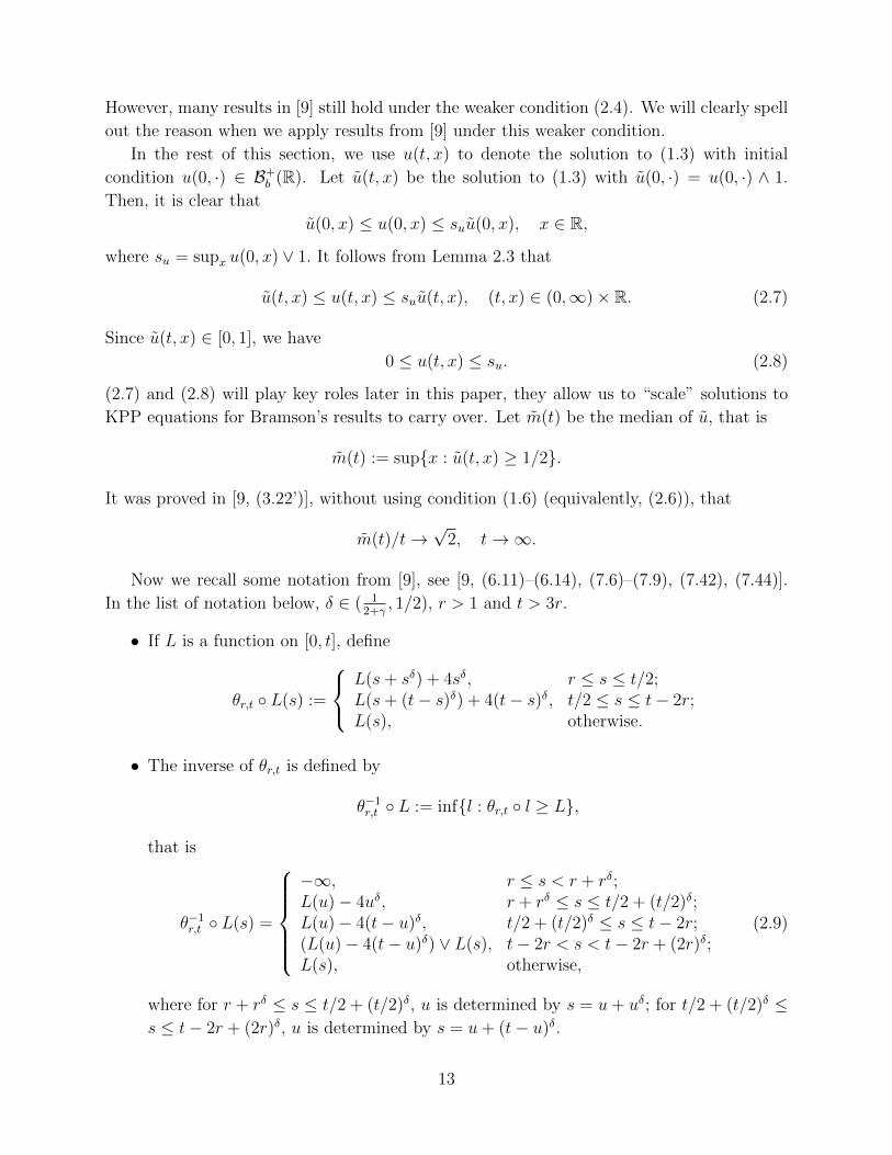
However, many results in [9] still hold under the weaker condition (2.4). We will clearly spell
out the reason when we apply results from [9] under this weaker condition.
In the rest of this section, we use u(t, x) to denote the solution to (1.3) with initial
condition u(0, ·) ∈ B+b (R). Let u(t, x) be the solution to (1.3) with u(0, ·) = u(0, ·) ∧ 1.
Then, it is clear that
u(0, x) ≤ u(0, x) ≤ suu(0, x), x ∈ R,
where su = supx u(0, x) ∨ 1. It follows from Lemma 2.3 that
u(t, x) ≤ u(t, x) ≤ suu(t, x), (t, x) ∈ (0,∞)× R. (2.7)
Since u(t, x) ∈ [0, 1], we have
0 ≤ u(t, x) ≤ su. (2.8)
(2.7) and (2.8) will play key roles later in this paper, they allow us to “scale” solutions to
KPP equations for Bramson’s results to carry over. Let m(t) be the median of u, that is
m(t) := sup{x : u(t, x) ≥ 1/2}.
It was proved in [9, (3.22’)], without using condition (1.6) (equivalently, (2.6)), that
m(t)/t→√
2, t→∞.
Now we recall some notation from [9], see [9, (6.11)–(6.14), (7.6)–(7.9), (7.42), (7.44)].
In the list of notation below, δ ∈ ( 12+γ
, 1/2), r > 1 and t > 3r.
• If L is a function on [0, t], define
θr,t ◦ L(s) :=
L(s+ sδ) + 4sδ, r ≤ s ≤ t/2;L(s+ (t− s)δ) + 4(t− s)δ, t/2 ≤ s ≤ t− 2r;L(s), otherwise.
• The inverse of θr,t is defined by
θ−1r,t ◦ L := inf{l : θr,t ◦ l ≥ L},
that is
θ−1r,t ◦ L(s) =
−∞, r ≤ s < r + rδ;L(u)− 4uδ, r + rδ ≤ s ≤ t/2 + (t/2)δ;L(u)− 4(t− u)δ, t/2 + (t/2)δ ≤ s ≤ t− 2r;(L(u)− 4(t− u)δ) ∨ L(s), t− 2r < s < t− 2r + (2r)δ;L(s), otherwise,
(2.9)
where for r + rδ ≤ s ≤ t/2 + (t/2)δ, u is determined by s = u+ uδ; for t/2 + (t/2)δ ≤s ≤ t− 2r + (2r)δ, u is determined by s = u+ (t− u)δ.
13
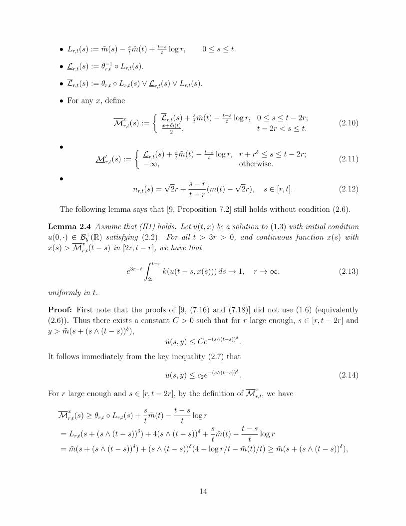
• Lr,t(s) := m(s)− stm(t) + t−s
tlog r, 0 ≤ s ≤ t.
• Lr,t(s) := θ−1r,t ◦ Lr,t(s).
• Lr,t(s) := θr,t ◦ Lr,t(s) ∨ Lr,t(s) ∨ Lr,t(s).
• For any x, define
Mx
r,t(s) :=
{Lr,t(s) + s
tm(t)− t−s
tlog r, 0 ≤ s ≤ t− 2r;
x+m(t)2
, t− 2r < s ≤ t.(2.10)
•M′
r,t(s) :=
{Lr,t(s) + s
tm(t)− t−s
tlog r, r + rδ ≤ s ≤ t− 2r;
−∞, otherwise.(2.11)
•nr,t(s) =
√2r +
s− rt− r
(m(t)−√
2r), s ∈ [r, t]. (2.12)
The following lemma says that [9, Proposition 7.2] still holds without condition (2.6).
Lemma 2.4 Assume that (H1) holds. Let u(t, x) be a solution to (1.3) with initial condition
u(0, ·) ∈ B+b (R) satisfying (2.2). For all t > 3r > 0, and continuous function x(s) with
x(s) >Mx
r,t(t− s) in [2r, t− r], we have that
e3r−t∫ t−r
2r
k(u(t− s, x(s))) ds→ 1, r →∞, (2.13)
uniformly in t.
Proof: First note that the proofs of [9, (7.16) and (7.18)] did not use (1.6) (equivalently
(2.6)). Thus there exists a constant C > 0 such that for r large enough, s ∈ [r, t − 2r] and
y > m(s+ (s ∧ (t− s))δ),u(s, y) ≤ Ce−(s∧(t−s))δ .
It follows immediately from the key inequality (2.7) that
u(s, y) ≤ c2e−(s∧(t−s))δ . (2.14)
For r large enough and s ∈ [r, t− 2r], by the definition of Mx
r,t, we have
Mx
r,t(s) ≥ θr,t ◦ Lr,t(s) +s
tm(t)− t− s
tlog r
= Lr,t(s+ (s ∧ (t− s))δ) + 4(s ∧ (t− s))δ +s
tm(t)− t− s
tlog r
= m(s+ (s ∧ (t− s))δ) + (s ∧ (t− s))δ(4− log r/t− m(t)/t) ≥ m(s+ (s ∧ (t− s))δ),
14
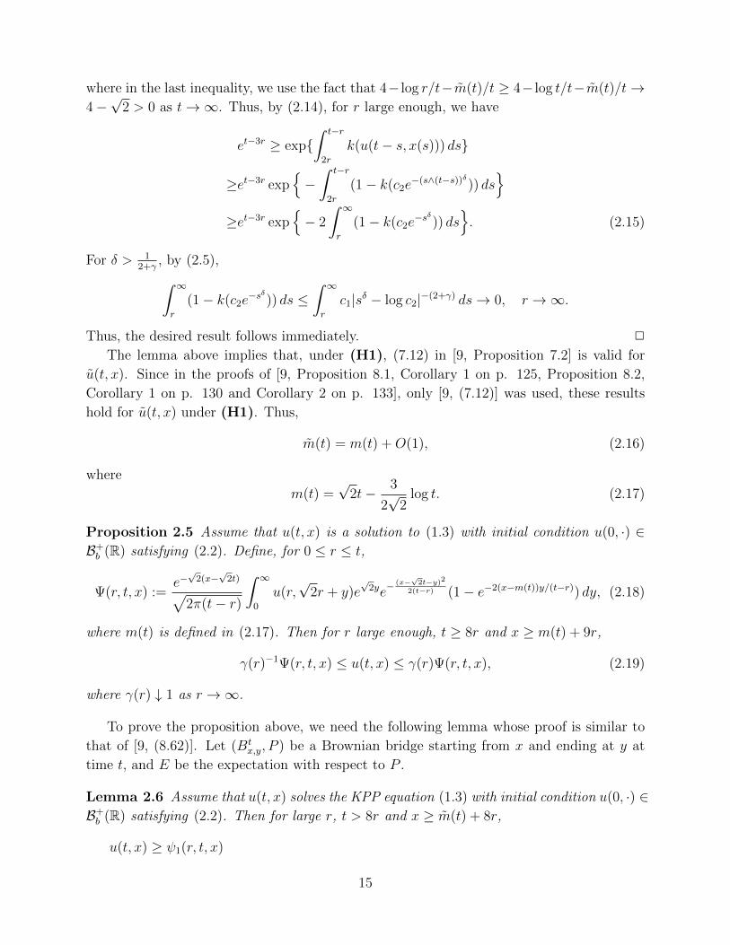
where in the last inequality, we use the fact that 4− log r/t−m(t)/t ≥ 4− log t/t−m(t)/t→4−√
2 > 0 as t→∞. Thus, by (2.14), for r large enough, we have
et−3r ≥ exp{∫ t−r
2r
k(u(t− s, x(s))) ds}
≥et−3r exp{−∫ t−r
2r
(1− k(c2e−(s∧(t−s))δ)) ds
}≥et−3r exp
{− 2
∫ ∞r
(1− k(c2e−sδ)) ds
}. (2.15)
For δ > 12+γ
, by (2.5),∫ ∞r
(1− k(c2e−sδ)) ds ≤
∫ ∞r
c1|sδ − log c2|−(2+γ) ds→ 0, r →∞.
Thus, the desired result follows immediately. 2
The lemma above implies that, under (H1), (7.12) in [9, Proposition 7.2] is valid for
u(t, x). Since in the proofs of [9, Proposition 8.1, Corollary 1 on p. 125, Proposition 8.2,
Corollary 1 on p. 130 and Corollary 2 on p. 133], only [9, (7.12)] was used, these results
hold for u(t, x) under (H1). Thus,
m(t) = m(t) +O(1), (2.16)
where
m(t) =√
2t− 3
2√
2log t. (2.17)
Proposition 2.5 Assume that u(t, x) is a solution to (1.3) with initial condition u(0, ·) ∈B+b (R) satisfying (2.2). Define, for 0 ≤ r ≤ t,
Ψ(r, t, x) :=e−√
2(x−√
2t)√2π(t− r)
∫ ∞0
u(r,√
2r + y)e√
2ye−(x−√2t−y)2
2(t−r) (1− e−2(x−m(t))y/(t−r)) dy, (2.18)
where m(t) is defined in (2.17). Then for r large enough, t ≥ 8r and x ≥ m(t) + 9r,
γ(r)−1Ψ(r, t, x) ≤ u(t, x) ≤ γ(r)Ψ(r, t, x), (2.19)
where γ(r) ↓ 1 as r →∞.
To prove the proposition above, we need the following lemma whose proof is similar to
that of [9, (8.62)]. Let (Btx,y, P ) be a Brownian bridge starting from x and ending at y at
time t, and E be the expectation with respect to P .
Lemma 2.6 Assume that u(t, x) solves the KPP equation (1.3) with initial condition u(0, ·) ∈B+b (R) satisfying (2.2). Then for large r, t > 8r and x ≥ m(t) + 8r,
u(t, x) ≥ ψ1(r, t, x)
15
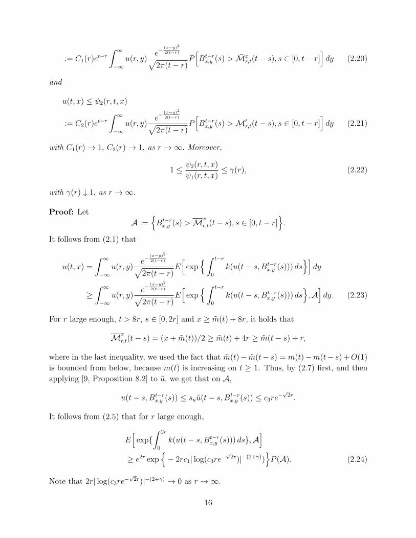
:= C1(r)et−r∫ ∞−∞
u(r, y)e−
(x−y)22(t−r)√
2π(t− r)P[Bt−rx,y (s) > Mx
r,t(t− s), s ∈ [0, t− r]]dy (2.20)
and
u(t, x) ≤ ψ2(r, t, x)
:= C2(r)et−r∫ ∞−∞
u(r, y)e−
(x−y)22(t−r)√
2π(t− r)P[Bt−rx,y (s) >M′
r,t(t− s), s ∈ [0, t− r]]dy (2.21)
with C1(r)→ 1, C2(r)→ 1, as r →∞. Moreover,
1 ≤ ψ2(r, t, x)
ψ1(r, t, x)≤ γ(r), (2.22)
with γ(r) ↓ 1, as r →∞.
Proof: Let
A :={Bt−rx,y (s) >Mx
r,t(t− s), s ∈ [0, t− r]}.
It follows from (2.1) that
u(t, x) =
∫ ∞−∞
u(r, y)e−
(x−y)22(t−r)√
2π(t− r)E[
exp{∫ t−r
0
k(u(t− s, Bt−rx,y (s))) ds
}]dy
≥∫ ∞−∞
u(r, y)e−
(x−y)22(t−r)√
2π(t− r)E[
exp{∫ t−r
0
k(u(t− s, Bt−rx,y (s))) ds
},A]dy. (2.23)
For r large enough, t > 8r, s ∈ [0, 2r] and x ≥ m(t) + 8r, it holds that
Mx
r,t(t− s) = (x+ m(t))/2 ≥ m(t) + 4r ≥ m(t− s) + r,
where in the last inequality, we used the fact that m(t)− m(t− s) = m(t)−m(t− s) +O(1)
is bounded from below, because m(t) is increasing on t ≥ 1. Thus, by (2.7) first, and then
applying [9, Proposition 8.2] to u, we get that on A,
u(t− s, Bt−rx,y (s)) ≤ suu(t− s, Bt−r
x,y (s)) ≤ c3re−√
2r.
It follows from (2.5) that for r large enough,
E[
exp{∫ 2r
0
k(u(t− s, Bt−rx,y (s))) ds},A
]≥ e2r exp
{− 2rc1| log(c3re
−√
2r)|−(2+γ))}P (A). (2.24)
Note that 2r| log(c3re−√
2r)|−(2+γ) → 0 as r →∞.
16
By Lemma 2.4, we have
E[
exp{∫ t−r
2r
k(u(t− s, Bt−rx,y (s))) ds},A
]≥et−3r
∫ ∞r
c1|sδ − log c2|−(2+γ) dsP (A). (2.25)
Combining (2.23)–(2.25), we immediately get (2.20). The proof of (2.21) is similar to that
of [9, Proposition 8.3 (b)] and the proof of (2.22) is similar to that of [9, (8.62)]. Here we
omit the details. 2
Proof of Proposition 2.5: Recall that nr,t(·) is defined by (2.12). First, we claim that, for
s ∈ [r, t],
M′r,t(s) ≤ nr,t(s) ≤M
x
r,t(s). (2.26)
It has been proved in [9, Lemma 2.2] that for y >√
2r and x > m(t),
P[Bt−rx,y (s) > nr,t(t− s), s ∈ [0, t− r]
]=P[Bt−r
0,0 (s) > − s
t− r(y −
√2r)− t− r − s
t− r(x−m(t)), s ∈ [0, t− r]
]=1− exp
{− 2(x−m(t))(y −
√2r)
t− r
},
and for y ≤√
2r, P[Bt−rx,y (s) > nr,t(t − s), s ∈ [0, t − r]
]= 0. Thus, combining Lemma 2.6
and (2.26), the desired result follows immediately.
Now we prove the claim. For r large enough, s ∈ [r + rδ, t/2] and u determined by
s = u+ uδ,
M′r,t(s) = Lr,t(u)− 4uδ +
s
tm(t)− t− s
tlog r
= m(u)− uδ(4− log r + m(t)
t) ≤ m(u) ≤ m(s),
where in the last inequality we used that fact m(t) is increasing for t large enough. Similarly,
for s ∈ [t/2, t− 2r], M′r,t(s) ≤ m(s). Thus, for all s ∈ [0, t], M′
r,ts) ≤ m(s).
By the definition of nr,t(s), for r large enough,
nr,t(s) =√
2r +s− rt− r
(m(t)−√
2r) =√
2s− s− rt− r
3
2√
2log t ≥ m(s),
where we used the fact that for large r, t → log t/(t − r) is decreasing. Thus, we get that
M′r,t(s) ≤ nr,t(s), s ∈ [r, t].
Now we deal with Mx
r,t(s). For r large enough, s ∈ [r, t/2],
Mx
r,t(s) ≥ m(s+ sδ)) ≥√
2s ≥ nr,t(s).
17
For r large enough, s ∈ [t/2, t− 2r],
Mx
r,t(s) ≥ m(s+ (t− s)δ) ≥√
2s+√
2(t− s)δ − 3
2√
2log t ≥ nr,t(s).
For r large enough, s ∈ [t− 2r, t] and x ≥ m(t) + 9r,
Mx
r,t(s) =m(t) + x
2≥ m(t) ≥ nr,t(s),
where the last inequality follows from the fact that, for r large enough,√
2r ≤ m(t). The
proof is now complete. 2
3 Proof of main results
We first give a useful lemma. The proof of this lemma will be given in Section 5.
Lemma 3.1 Assume that (H1) and (H3) hold. Then, for any t > 0 and θ > 0, we have
that V (t, ·) ∈ B+b (R), and ∫ ∞
0
V (t, x)xeθx dx <∞.
Corollary 3.2 Assume that (H1) and (H3) hold. If φ ∈ B+(R) satisfies the integrability
condition (1.19) at −∞ and if there exists x0 < 0 such that φ is bounded on (−∞, x0], then
for any t > 0, we have that Uφ(t, ·) and Vφ(t, ·) are bounded functions satisfying (2.2).
Proof: First, we assume that φ ∈ B+b (R) and satisfies the integrability condition (1.19) at
−∞. Note that Uφ(t, x) satisfies the KPP equation (1.3) with Uφ(0, x) = φ(−x) ∈ B+b (R)
satisfying the integrability condition (2.2) at ∞, thus by Lemma 2.1, Uφ(t, x) is bounded
and satisfies (2.2). For Vφ(t, x), it is clear that, by Lemma 2.3.(2),
Vφ(t, x) = limθ→∞
Uφ+θ1(0,∞)(t, x)
≤ Uφ(t, x) + limθ→∞
Uθ1(0,∞)(t, x) ≤ Uφ(t, x) + V (t, x),
where V is defined in (1.17). By Lemma 3.1, V (t, x) is bounded and satisfies the integrability
condition (2.2) at ∞. Thus Vφ is a bounded function satisfying the integrability condition
(2.2) at ∞, when φ ∈ B+b (R) and satisfies the integrability condition (1.19) at −∞.
Now we assume that φ ∈ B+(R) satisfies the integrability condition (1.19) at −∞ and
that there exists x0 < 0 such that φ is bounded on (−∞, x0]. Let φ(x) := φ(x)1x≤x0 ∈ B+b (R).
Note that
Vφ(t, x) ≤ − logE[
exp{−∫Rφ(y − x)Xt(dy)
},Mt ≤ x+ x0
]= Vφ(·+x0)(t, x+ x0).
Thus Vφ is a bounded function satisfying the integrability condition (2.2) at ∞. Since
Uφ(t, x) ≤ Vφ(t, x), Uφ is also a bounded function satisfying the integrability condition (2.2)
at ∞. 2
18
3.1 Large deviation results
Proof of Proposition 1.1: (1) Let Ψ be defined by (2.18) with u replaced by Uφ. We
claim that
limt→∞
e√
2x t3/2
32√
2log t
Ψ(r, t,√
2t+ x) =
√2
π
∫ ∞0
Uφ(r,√
2r + y)ye√
2y dy := C(φ, r). (3.1)
Note that, for r > 1 and t ≥ 8r,
e√
2x t3/2
32√
2log t
e−√
2x√2π(t− r)
Uφ(r,√
2r + y)e√
2ye−(x−y)22(t−r)
(1− e−2(x+ 3
2√2
log t)y/(t−r))
≤ c(1 + |x|)Uφ(r,√
2r + y)ye√
2y.
By (2.3), the right hand side of the inequality above is integrable. So by the dominated
convergence theorem, we get that the claim is true and that C(φ, r) ∈ (0,∞).
Since Uφ is the solution to (1.3) with Uφ(0, x) = φ(−x) satisfying the integrability con-
dition (2.2) at ∞, by Proposition 2.5, for r large enough, t ≥ 8r and x ≥ − 32√
2log t+ 9r,
γ(r)−1Ψ(r, t,√
2t+ x) ≤ Uφ(t,√
2t+ x) ≤ γ(r)Ψ(r, t,√
2t+ x).
Thus, by (3.1), we have
γ(r)−1C(φ, r) ≤ lim inft→∞
e√
2x t3/2
32√
2log t
Uφ(t,√
2t+ x)
≤ lim supt→∞
e√
2x t3/2
32√
2log t
Uφ(t,√
2t+ x) ≤ γ(r)C(φ, r). (3.2)
Letting r →∞, by the fact that limr→∞ γ(r) = 1, we get that
lim supr→∞
C(φ, r) ≤ lim inft→∞
e√
2x t3/2
32√
2log t
Uφ(t,√
2t+ x)
≤ lim supt→∞
e√
2x t3/2
32√
2log t
Uφ(t,√
2t+ x) ≤ lim infr→∞
C(φ, r).
It follows that C(φ) := limr→∞C(φ, r) exists, and then (1.20) follows immediately. Now we
show that C(φ) ∈ (0,∞) if φ is non-trivial. In fact, by (3.2), we have
0 < γ(r)−1C(φ, r) ≤ C(φ) ≤ γ(r)C(φ, r) <∞.
For any z, it is clear that Uθ−zφ(t, x) = Uφ(t, x+ z), which implies that
C(φ)e−√
2ze−√
2x = limt→∞
t3/2
32√
2log t
Uφ(t,√
2t+ x+ z) = C(θ−zφ)e−√
2x,
19
which further implies that C(θ−zφ) = C(φ)e−√
2z, that is
C(θ−zφ) = limr→∞
√2
π
∫ ∞0
Uφ(r,√
2r + y + z)ye√
2y dy = C(φ)e−√
2z. (3.3)
(2) Recall that in this part we assume that (H1) and (H3) hold, and φ ∈ B+(R) satisfies
the integrability condition (1.19) at −∞ and that there exists x0 < 0 such that φ is bounded
on (−∞, x0]. Note that , for t0 > 0, Uφ(t + t0, x +√
2t0) and Vφ(t + t0, x +√
2t0) are the
solution to (1.3) with initial data Uφ(t0, x +√
2t0) and Vφ(t0, x +√
2t0) respectively. By
Corollary 3.2, we have that Uφ(t0, x +√
2t0) and Vφ(t0, x +√
2t0) are bounded and satisfy
the integrability condition (2.2) at ∞. It follows from (1.20) that
limt→∞
t3/2
32√
2log t
Vφ(t, x+√
2t) = limt→∞
t3/2
32√
2log t
Vφ(t+ t0, x+√
2t0 +√
2t) = Ce−√
2x,
where
C = limr→∞
√2
π
∫ ∞0
Vφ(r + t0,√
2r +√
2t0 + y)ye√
2y dy
= limr→∞
√2
π
∫ ∞0
Vφ(r,√
2r + y)ye√
2y dy := C(φ).
Similarly,
limt→∞
t3/2
32√
2log t
Uφ(t, x+√
2t) = C(φ)e−√
2x.
The proof is now complete. 2
Proof of Theorem 1.2: It is clear that (1.22) follows from (1.21) with φ = 0. Now we
prove (1.23). For t0 > 0, using Proposition 2.5 with u(0, x) = V (t0,√
2t0 + x), we get that
γ(r)−1Ψ(r, t, x) ≤ V (t0 + t,√
2t0 + x) ≤ γ(r)Ψ(r, t, x).
By Lemma 3.1 and the dominated convergence theorem, we have that
limt→∞
√te(δ2/2+
√2δ)tΨ(r, t, (
√2 + δ)t+ x)
=
√2
πδe−(δ+
√2)xe−
12δ2r
∫ ∞0
V (t0 + r,√
2r +√
2t0 + y)ye(√
2+δ)y dy ∈ (0,∞).
Now, using arguments similar to that used in the proof of Proposition 1.1 (1), we get that
limt→∞
√te(δ2/2+
√2δ)tV (t0 + t, (
√2 + δ)t+
√2t0 + x)
=
√2
πδe−(δ+
√2)x lim
r→∞e−
12δ2r
∫ ∞0
V (t0 + r,√
2r +√
2t0 + y)ye(√
2+δ)y dy
=
√2
πδe
12δ2t0e−(δ+
√2)x lim
r→∞e−
12δ2r
∫ ∞0
V (r,√
2r + y)ye(√
2+δ)y dy ∈ (0,∞),
20

where the limit above exists. Letting x = δt0, we get that
limt→∞
√te(δ2/2+
√2δ)tV (t, (
√2 + δ)t)
=
√2
πδ limr→∞
e−12δ2r
∫ ∞0
V (r,√
2r + y)ye(√
2+δ)y dy := C(δ).
It follows that
limt→∞
√te(δ2/2+
√2δ)tP(Mt > (
√2 + δ)t) = C(δ).
2
3.2 The extremal process
In this subsection we give the proofs of our main results–Theorems 1.3, 1.6 and 1.7. Recall
that m(t) is defined in (2.17).
3.2.1 Proofs of Theorems 1.3 and 1.6
Proof of Theorem 1.3: (1) In this part, we assume that φ is bounded and satisfies (1.19).
Define
wφ(x) := − logE(e−C(φ)Z∞e−√2x
). (3.4)
Recall that (cf. (1.13)–(1.14)) w is a traveling wave to (1.3) and satisfies
limx→∞
wφ(x)
xe−√
2x= C(φ). (3.5)
Let Ψ be defined by (2.18) with u replaced by Uφ. We claim that, for any positive function
z(t) with limt→∞ z(t) = z > 0,
limt→∞
Ψ(r, t, z(t) +m(t)) = C(φ, r)ze−√
2z. (3.6)
In fact, for any t ≥ 8r and y ≥ 0,
z(t)−1 t3/2√2π(t− r)
Uφ(r,√
2r + y)e√
2ye−(z(t)+m(t)−
√2t−y)2
2(t−r)(1− e−2z(t)y/(t−r))
≤ cUφ(r,√
2r + y)ye√
2y. (3.7)
Thus, we can apply the dominated convergence theorem to get that
limt→∞
z(t)−1e√
2z(t)Ψ(r, t, z(t) +m(t)) = C(φ, r),
which is the same as (3.6). Put
f (r,t)(x) = |Ψ(r, t, x+m(t))− C(φ, r)xe−√
2x|, x > 0.
21

It follows from the key inequality (2.8) that Uφ(t, x) ≤ (‖φ‖∞ ∨ 1). Applying Proposition
2.5, we get that, for r large enough, x > 9r and t ≥ 8r,
Uφ(t,m(t) + x) ≤ γ(r)Ψ(r, t, x+m(t)).
Thus, for any t ≥ 8r,
Uφ(t,m(t) + x) ≤ γ(r)C(φ, r)xe−√
2x1x>9r + γ(r)f (r,t)(x)1x>9r + (‖φ‖∞ ∨ 1)1x≤9r.
Let u1,r(s, x), u2,r(s, x) and vr,t(s, x) be the solutions to the KPP equation (1.3) with initial
conditions C(φ)xe−√
2x1x>9r, (‖φ‖∞ ∨ 1)1x≤9r and γ(r)f (r,t)(x)1x>9r respectively. Then, by
Lemma 2.3, we have
Uφ(t+ s,m(t) + x) ≤(γ(r)C(φ, r)
C(φ)∨ 1
)u1,r(s, x) + u2,r(s, x) + vr,t(s, x).
Let a(r) := γ(r)C(φ,r)C(φ)
∨ 1. Applying (2.1) with r = 0 and using the fact that k(λ) ≤ 1, we get
that
vr,t(s, x) ≤ esγ(r)Ex(f(r,t)(Bs)1Bs>9r).
Thus,
Uφ(t+ s,m(t+ s) + x(t+ s))
≤a(r)u1,r(s, x(t+ s) +m(t+ s)−m(t)) + u2,r(s, x(t+ s) +m(t+ s)−m(t))
+ esγ(r)E(f (r,t)(m(t+ s)−m(t) + x(t+ s) +Bs),m(t+ s)−m(t) + x(t+ s) +Bs > 9r).
Letting t→∞ and using (3.6), we get
lim supt→∞
Uφ(t,m(t) + x(t)) ≤ a(r)u1,r(s, x+√
2s) + u2,r(s, x+√
2s).
Since (‖φ‖∞∨1)1x<9r satisfies (2.2), we have by Proposition 1.1.(1) that u2,r(s, x+√
2s)→ 0
as s → ∞. Since C(φ)xe−√
2x/wφ(x) → 1 as x → ∞, by [9, Lemma 3.4] (Note that our
(1.14), which is exactly [9, (1.13)], holds under (H1)-(H2), thus [9, Lemma 3.4] holds under
(H1)-(H2)), we get that
u1,r(s, x+√
2s)→ wφ(x), s→∞.
Now letting s→∞ and then r →∞, we get that
lim supt→∞
Uφ(t,m(t) + x(t)) ≤ limr→∞
a(r)wφ(x) = wφ(x).
On the other hand,
γ(r)−1C(φ, r)xe−√
2x1x>9r ≤ Uφ(t,m(t) + x) + γ(r)−1f (r,t)(x)1x>9r.
22
Using arguments similar as above, we can get that
lim inft→∞
Uφ(t,m(t) + x(t)) ≥ wφ(x).
Therefore, we have
limt→∞
Uφ(t,m(t) + x(t)) = wφ(x). (3.8)
(2) Recall that, in this part, φ is not necessarily bounded. Applying (3.8) to (t, x) →Vφ(t+ t0,
√2t0 + x) and Proposition 1.1 (2), we get that
limt→∞
Vφ(t+ t0,m(t) +√
2t0 + x(t)) = − logE(e−C(φ)Z∞e−√2x
).
Since m(t+ t0)−m(t)−√
2t0 + x(t)→ x, we get that
limt→∞
Vφ(t+ t0,m(t+ t0) + x(t)) = − logE(e−C(φ)Z∞e−√2x
),
which implies the desired result. Similarly, applying Corollary 3.2 and (3.8) to (t, x) →Uφ(t + t0,
√2t0 + x), it is clear that (3.8) also holds for φ ∈ B+(R). The proof is now
complete. 2
Using Theorem 1.3, we get the convergence of the Laplace transforms. To obtain weak
convergence, we need to show the continuity of C(φ) and C(φ).
Lemma 3.3 Assume that (H1) and (H2) hold. Then for any φ ∈ H,
limλ↓0
C(λφ) = C(0) = 0. (3.9)
If, in addition, (H3) holds, then for any φ ∈ H,
limλ↓0
C(λφ) = C0. (3.10)
Proof: For any φ ∈ H, choose mφ such that φ(x) = 0 for all x < mφ. Then we have for all
N > 0,
E(exp{−λ〈φ, Et〉}) ≥ E(exp{−λ‖φ‖∞Et(mφ,∞)}) ≥ e−λ‖φ‖∞NP(Et(mφ,∞) ≤ N).
Letting t → ∞, λ → 0 and then N → ∞, by Theorem 1.3 we see that, to prove (3.9), it
suffices to show that
limN→∞
lim supt→∞
P(Et(mφ,∞) > N) = 0. (3.11)
Let g(x) = 1(0,∞)(x), then ug(t, x) = − logE(exp{−Xt(−x,∞)}) is increasing on x. For any
n ≥ 1,
E(Et(mφ,∞) > N, exp{−〈θ−ng, Et+1})
= E(Et(mφ,∞) > N,EXt
(exp
{−∫g(y − n−m(t+ 1))X1(dy)
}))23
= E(Et(mφ,∞) > N, exp
{−∫ug(1, x− n−m(t+ 1) +m(t))Et(dx)
})≤ E
(Et(mφ,∞) > N, exp
{− ug(1,mφ − n−m(t+ 1) +m(t))Et(mφ,∞)
})≤ exp{−ug(1,mφ − n−m(t+ 1) +m(t))N}.
Thus, we get that
lim supt→∞
P(Et(mφ,∞) > N)
≤ lim supt→∞
E(Et(mφ,∞) > N, exp{−〈θ−ng, Et+1})
+ 1− limt→∞
E(exp{−〈θ−ng, Et+1})
≤ exp{−ug(1,mφ − n−√
2)N}+ 1− E(exp{−C(g)e−√
2nZ∞}).
Letting N →∞ and then n→∞, (3.11) follows immediately. Thus (3.9) is valid.
Now we prove (3.10) under the additional assumption (H3). It is clear that
0 ≤ P(Mt −m(t) ≤ 0)− E(exp{−λ〈φ, Et〉},Mt −m(t) ≤ 0) ≤ 1− E(exp{−λ〈φ, Et〉}).
Thus, by (3.9) and Theorem 1.3.(2) with x(t) = 0, we get that
E(exp{− limλ→0
C(λφ)Z∞}) = E(exp{−C0Z∞}).
Now (3.10) follows immediately. The proof is now complete. 2
For any t > 0, we define Et := T−√2tXt.
Proposition 3.4 Assume that (H1) and (H3) hold. For any z ∈ R, conditioned on {Mt >√2t+z}, (Et−z,Mt−
√2t−z) converges in distribution to a limit (independent of z) (E∞, Y ),
where Y is an exponential random variable with parameter√
2 and for any φ ∈ C+c (R),
E[
exp{−∫Rφ(y)E∞(dy)
}, Y > x
]=C(θxφ)e−
√2x − C(φ)
C0
, x > 0.
Moreover,
(Xt −Mt,Mt −√
2t− z)|Mt>√
2t+z
converges in law to (∆, Y ), where the random measure ∆ = E∞ − Y is independent of Y .
Remark 3.5 Define Yt := Xt(√
2t,∞) = 〈h, Et〉, where h(x) = 1(0,∞)(x). It follows from
Proposition 3.4 that Yt|Yt>0 converges weakly.
Proof of Proposition 3.4: First, we show that Mt−√
2t− z|Mt>√
2t+z converges in distri-
bution to an exponential random variable with parameter√
2. In fact, by (1.21) with φ = 0,
we get that for any x > 0,
limt→∞
P(Mt −√
2t− z > x|Mt >√
2t+ z) = limt→∞
t3/23
2√2
log tP(Mt >
√2t+ z + x)
t3/23
2√2
log tP(Mt >
√2t+ z)
= e−√
2x.
24
For any x > 0 and φ ∈ B+b (R) satisfying the integrability condition (1.19) at −∞, applying
Proposition 1.1 several times, we get
limt→∞
E(e−
∫R φ(y−
√2t−z)Xt(dy),Mt >
√2t+ z + x|Mt >
√2t+ z
)= lim
t→∞
E(e−
∫R φ(y−
√2t−z)Xt(dy),Mt >
√2t+ z + x
)P(Mt >
√2t+ z)
= limt→∞
1− E(e−∫R φ(y−
√2t−z)Xt(dy),Mt ≤
√2t+ z + x)
P(Mt >√
2t+ z)− lim
t→∞
1− E(e−∫R φ(y−
√2t−z)Xt(dy))
P(Mt >√
2t+ z)
= limt→∞
Vθxφ(t,√
2t+ z + x)
V (t,√
2t+ z)− lim
t→∞
Uφ(t,√
2t+ z)
V (t,√
2t+ z)
=C(θxφ)e−
√2x − C(φ)
C0
,
where in the second to last equality above, we used L’Hospital’s rule and the facts that
Vθxφ(t,√
2t + z + x) → 0 and Uφ(t,√
2t + z) → 0 (which are consequences of (1.21) and
(1.20) respectively). Now applying Lemma 3.3, we get that for any φ ∈ C+c (R),
(〈φ, Et − z〉,Mt −√
2t− z)|Mt>√
2t+z
converges jointly in distribution. Thus the limit has the form (〈φ, E∞〉, Y ) (independent of
z), where the random measure E∞ ∈MR(R).
It follows by [5, Lemma 4.13] that, conditioned on Mt >√
2t + z, Xt −Mt converges in
law to E∞ − Y . Thus,
E(e−
∫R φ(y−Mt)Xt(dy),Mt −
√2t− z > x|Mt >
√2t+ z
)= E
(e−
∫R φ(y−Mt)Xt(dy)|Mt >
√2t+ z + x
)P(Mt >
√2t+ z + x|Mt >
√2t+ z)
→ E(e−∫R φ(y−Y ) E∞(dy))P(Y > x).
The desired independence result follows immediately. 2
Proof of Theorem 1.6: The weak convergence of Et and (1.27) follow immediately from
Theorem 1.3 (1) and Lemma 3.3. Now we assume that (H3) also holds and prove the second
assertion of Theorem 1.6. For any φ ∈ C+c (R), choose mφ such that φ(y) = 0 for all y < mφ.
Then we have
C(φ)
C0
= limt→∞
1− E[e−
∫φ(y−
√2t)Xt(dy)
]P(Mt >
√2t)
= limt→∞
E[1− e−
∫φ(y−
√2t)Xt(dy),Mt >
√2t+mφ
]P(Mt >
√2t)
= limt→∞
E[1− e−
∫φ(y−
√2t)Xt(dy)|Mt >
√2t+mφ
]P(Mt >√
2t+mφ)
P(Mt >√
2t)
25
= e−√
2mφ limt→∞
E[1− e−
∫φ(y+mφ−
√2t−mφ)Xt(dy)|Mt >
√2t+mφ
]= e−
√2mφE
[1− e−
∫φ(y+mφ) E∞(dy)
]= e−
√2mφ
∫ ∞0
√2e−
√2xE[1− e−
∫φ(y+mφ+x) ∆(dy)
]dx
=
∫ ∞−∞
√2e−
√2xE[1− e−
∫φ(y+x) ∆(dy)
]dx, (3.12)
where in the first, fifth and sixth equality we used Proposition 3.4, and in the fourth equality
we used Proposition 1.1. By the definition of∑
j ∆j(dx+ ej), we deduce that
E(e−
∑j φ(y+ej)∆j(dy)
)= E
∏j
[E(e−
∫φ(y+x)∆(dy)
)]x=ej
= exp
{−∫ (
1− E(e−
∫φ(y+x)∆(dy)
))C0Z∞
√2e−
√2x dx
}= exp{−C(φ)Z∞}. (3.13)
The proof is now complete. 2
3.2.2 Proof of Theorem 1.7
Lemma 3.6 Assume that (H1) and (H3) hold, and that φ ∈ B+(R) satisfies the integrabil-
ity condition (1.19) at −∞ and that there exists x0 < 0 such that φ is bounded on (−∞, x0].
Then
lims→∞
limt→∞
E[e−
∫φ(y−m(t)− 1√
2logZs)Xt(dy)
e−θZs , Zs > 0]
= e−C(φ)E[e−θZ∞ , Z∞ > 0
].
Proof: By the Markov property, we have for s < t,
E[
exp{−∫φ(y −m(t)− 1√
2logZs)Xt(dy)
}exp{−θZs}, Zs > 0
]= E
[exp
{−∫Uφ(t− s,m(t) +
1√2
logZs − y)Xs(dy)}
exp{− θZs
}, Zs > 0
].
Now applying Theorem 1.3 (2) and (3.4), we get that as t→∞,
E[
exp{−∫φ(y −m(t)− 1√
2logZs)Xt(dy)
}exp{−θZs}, Zs > 0
]→ E
[exp
{−∫wφ(√
2s+1√2
logZs − y)Xs(dy)}
exp{− θZs
}, Zs > 0
].
For any L > 0, define A(s, L) := {Zs > 0, logZs ∈ [−L,L],Ms ≤√
2s− log s}. Then
E[
exp{−∫wφ(√
2s+1√2
logZs − y)Xs(dy)}
exp{− θZs
}, Zs > 0
]≤ E
[exp
{−∫wφ(√
2s+1√2
logZs − y)Xs(dy)}
exp{− θZs
}, A(s, L)
]+ P(Zs > 0, | logZs| > L) + P(Ms >
√2s− log s) := (I) + (II) + (III).
26
Since {Z∞ = 0} = Sc and {Z∞ > 0} = S a.s., we have
limL→∞
lim sups→∞
P(Zs > 0, | logZs| > L)
≤ limL→∞
lim sups→∞
(P(Zs > 0, | logZs| > L,S) + P(Xs 6= 0,Sc)
)≤ lim
L→∞P(| logZ∞| ≥ L,S) = 0. (3.14)
By (1.26), we have
lims→∞
P(Ms >√
2s− log s) = 0. (3.15)
Now we consider (I). Sincewφ(x)
xe−√2x→ C(φ), as x → ∞, and on A(s, L), for y ∈ supp Xs,√
2s+ 1√2
logZs− y ≥ log s−L/√
2, thus for any ε > 0, there exists N such that for s > N ,
(1− ε)C(φ)
∫(√
2s+1√2
logZs − y)e−√
2(√
2s+ 1√2
logZs−y)Xs(dy)
≤∫wφ(√
2s+1√2
logZs − y)Xs(dy)
≤ (1 + ε)C(φ)
∫(√
2s+1√2
logZs − y)e−√
2(√
2s+ 1√2
logZs−y)Xs(dy).
Note that on A(s, L), for s large enough, | logZs|√2(√
2s−y)≤ L√
2 log s≤ ε. Thus (I) is less than or
equal to
E[
exp{− (1− ε)2C(φ)(Zs)
−1
∫(√
2s− y)e−√
2(√
2s−y)Xs(dy)}
exp{− θZs
}, A(s, L)
]≤ exp
{− (1− ε)2C(φ)
}E[
exp{− θZs
}, Zs > 0
]. (3.16)
Similarly,
(I) ≥ exp{− (1 + ε)2C(φ)
}E[
exp{− θZs
}, A(s, L)
]. (3.17)
Combining (3.14)–(3.17), letting s→∞, then L→∞, and then ε→ 0, we get that
lims→∞
E[
exp{−∫wφ(√
2s+1√2
logZs − y)Xs(dy)}
exp{− θZs
}, Zs > 0
]= exp
{− C(φ)
}E[
exp{− θZ∞
}, Z∞ > 0
].
The proof is now complete. 2
Proof of Theorem 1.7: Using arguments similar to that leading to (3.13), we get that for
any φ ∈ C+c (R),
E(e−
∑j φ(y+e′j)∆j(dy)
)= exp
{−∫ (
1− E(e−
∫φ(y+x)∆(dy)
))C0
√2e−
√2x dx
}= exp{−C(φ)}.
27

Since Zt → Z∞, we only need to prove that, for any φ ∈ C+c (R) and θ ≥ 0,
limt→∞
E[e−
∫φ(y)E∗t (dy)e−θZ∞ , Z∞ > 0
]= exp{−C(φ)}E[exp{−θZ∞}, Z∞ > 0]. (3.18)
Step 1 Define, for any b > 1,
gb(x) :=
0, |x| > b;1, |x| < b− 1;linear, otherwise.
It is clear that |gb(x)− gb(y)| ≤ |x− y|.First, we consider φ(x) = |f(x)|gb(x) where f(x) =
∑ni=1 θie
βix and θi, βi ∈ R. Let
f(x) :=∑n
i=1 |θi|eβix. It is clear that φ ∈ C+c (R). By Lemma 3.6, to prove (3.18), it suffices
to show that
lims→∞
lim supt→∞
∣∣∣E[e− ∫φ(y−m(t)− 1√
2logZ∞)Xt(dy)
e−θZ∞ , Z∞ > 0]
− E[e−
∫φ(y−m(t)− 1√
2logZs)Xt(dy)
e−θZs , Zs > 0]∣∣∣ = 0. (3.19)
For any K > 0 and M > 0, let fM
(y) = f(y)1|y|≤M+b and
A(s, t,K,M) = {〈fM , Et〉 > K} ∪{
1√2| logZ∞| > M
}∪{
1√2| logZs| > M
}.
Since 〈fM , Et〉 converges weakly and Zs → Z∞, a.s., for any ε > 0, there exist K,M such
that
lims→∞
lim supt→∞
P(A(s, t,K,M), Z∞ > 0) < ε. (3.20)
Note that, if |y| > |x1| ∨ |x2|+ b, φ(y − x1)− φ(y − x2) = 0; otherwise,
|φ(y − x1)− φ(y − x2)|≤ |f(y − x1)− f(y − x2)|+ |f(y − x2)||gb(y − x1)− gb(y − x2)|
≤ f(y)
[∑j
|e−βjx1 − e−βjx2|+∑j
e−βjx2|x1 − x2|
]=: f(y)H(x1, x2).
By the inequality |e−x − e−y| ≤ 1− e−|x−y| for any x, y > 0, we get that on A(s, t,K,M)c ∩{Zs > 0, Z∞ > 0},∣∣∣e− ∫
φ(y−m(t)− 1√2
logZ∞)Xt(dy)e−θZ∞ − e−
∫φ(y−m(t)− 1√
2logZs)Xt(dy)
e−θZs∣∣∣
≤ 1− exp{− θ|Zs − Z∞| − 〈f
M, Et〉H
(1√2
logZ∞,1√2
logZs
)}≤ 1− exp
{− θ|Zs − Z∞| −KH
(1√2
logZ∞,1√2
logZs
)}.
28
Since Zs → Z∞, the left hand side of (3.19) is no more than
lims→∞
lim supt→∞
[P(Zs ≤ 0, Z∞ > 0) + P(A(s, t,K,M), Z∞ > 0)
+ E(
1− exp{− θ|Zs − Z∞| −KH
(1√2
logZ∞,1√2
logZs
)}, Zs > 0, Z∞ > 0
)]≤ ε.
Now (3.19) follows immediately. Thus, the result holds for φ(x) of the form specified at the
beginning of this step.
Step 2 We will show that (3.18) holds for φ ∈ C+c (R). Choose b > 1 such that φ(x) = 0
for |x| > b − 1. According to the Stone-Weierstrass theorem, for any n ≥ 1, there exists a
polynomial Qn,b such that
supy∈[e−b,eb]
|Qn,b(y)− φ(log y)| ≤ n−1,
which is equivalent to that
supy∈[−b,b]
|Qn,b(ey)− φ(y)| ≤ n−1.
Let φn,b(y) := |Qn,b(ey)|gb(y), it is clear that all the functions φn,b satisfy the conditions in
Step 1, and |φn,b(y)− φ(y)| ≤ n−1gb(y). Thus∣∣∣E[e− ∫φ(y)E∗t (dy)e−θZ∞ , Z∞ > 0
]− E
[e−
∫φn,b(y)E∗t (dy)e−θZ∞ , Z∞ > 0
]∣∣∣≤ E
[1− e−
∫|φ(y)−φn,b(y)|E∗t (dy), Z∞ > 0
]≤ E
[1− e−n−1
∫gb(y)E∗t (dy), Z∞ > 0
].
In Step 1, we have shown that,
limn→∞
limt→∞
E[1− e−n−1
∫gb(y)E∗t (dy), Z∞ > 0
]= lim
n→∞(1− exp{−C(n−1gb)})P(Z∞ > 0) = 0.
Thus we have
limt→∞
E[e−
∫φ(y)E∗t (dy)e−θZ∞ , Z∞ > 0
]= lim
n→∞limt→∞
E[e−
∫φn,b(y)E∗t (dy)e−θZ∞ , Z∞ > 0
]= lim
n→∞exp{−C(φn,b)}E
[e−θZ∞ , Z∞ > 0
].
Since |φn,b(y)− φ(y)| ≤ n−1gb(y), by Lemmas 2.3 and 3.3, we have
|C(φn,b)− C(φ)| ≤ C(n−1gb)→ 0, n→∞.
Thus, (3.18) is valid for all φ ∈ C+c (R). 2
29

In fact, it is not surprising that E∗∞ has the decomposition (1.29). A random measure M
is said to be exp-√
2-stable if any a, b satisfying e√
2a + e√
2b = 1, it holds that
TaM + TbMd= M,
where M is an independent copy of M . The following proposition shows that E∗∞ satisfies
the exp-√
2-stability:
Proposition 3.7 Under (H1) and (H3), E∗∞ satisfies the exp-√
2-stability.
Proof: The Laplace transform of TaE∗∞ is given by
E(exp{−〈φ, TaE∗∞}) = E(exp{−〈θaφ, E∗∞}) = exp{−C(θaφ)} = exp{−C(φ)e√
2a}, φ ∈ C+c (R).
Therefore, the desired result follows. 2
Remark 3.8 Let M1, . . . ,Mn be a sequence of i.i.d. random measures with the same law as
T− logn/√
2E∗∞. Then, by Proposition 3.7, E∗∞ is equal in law to M1 + · · · + Mn. Thus E∗∞ is
infinitely divisible. Applying [37, Theorem 3.1], we get that for any φ ∈ C+c (R),
C(φ) = − logE[exp{−〈φ, E∗∞〉}] =c
∫Rφ(x)e−
√2x dx
+
∫Re−√
2x
∫MR(R)\{0}
[1− exp{−〈φ, µ〉}] TxΛ(dµ) dx,
for some constant c > 0 and some measure Λ on MR(R) \ {0} with the property that for
every bounded Borel set A ⊂ R,∫Re−√
2x
∫MR(R)\{0}
[1 ∧ µ(A− x)]Λ(dµ) dx <∞.
Now we choose a function φ ∈ C+c (R) such that φ(x) = 0 for any x < 0. It is clear that
Uλφ(t, x) ≤ V (t, x). Under (H1) and (H3), it holds that C(λφ) ≤ C0 ∈ (0,∞) for any
λ > 0. This implies that c = 0. Thus
E∗∞d=∑j
TξjDj,
where∑
j δ(xj ,Dj) is Poisson point process with intensity measure e−√
2x dxΛ(dµ). Theorem
1.7 says that Λ(dµ) =√
2C0P(∆ ∈ dµ) where ∆ is the limit of Xt − Mt conditioned on
{Mt >√
2t}.
30

4 Proof of Lemma 3.1
In this section, we will give an upper estimate for − logPδx(Xs([−A,A]c = 0, 0 ≤ s ≤ t),
which implies Lemma 3.1. Pinsky [40] has proved a similar result for super-Brownian motions
with quadratic branching mechanism. Here we use the idea of [40] to generalize the result
to super-Brownian motions with more general branching mechanisms.
Lemma 4.1 (Maximum principle) Let ψ(λ) := −aλ+ bλ1+ϑ, where a > 0, b > 0, ϑ > 0.
Assume that v1(x) and v2(x) are two functions defined on (a1, a2) such that vi(x) ≥ (ab−1)1/ϑ,
i = 1, 2, v1(ai) ≤ v2(ai), i = 1, 2, and that
1
2
d2
dx2v2(x)− ψ(v2(x)) ≤ 1
2
d2
dx2v1(x)− ψ(v1(x)), x ∈ (a1, a2).
Then we have that
v1(x) ≤ v2(x), x ∈ (a1, a2).
Proof: The proof is a slight modification of the proof of [9, Proposition 3.1], using [41,
Theorem 3.4]. See also the proof of [7, Proposition 6.4]. We omit the details 2
Lemma 4.2 Let ψ(λ) := −aλ+ bλ1+ϑ, where a > 0, b > 0, ϑ ∈ (0, 1]. For any A > 0, there
exists an even function hA(x) on (−A,A) such that
1
2∆hA(x) = ψ(hA(x)), |x| < A, (4.1)
and that limx→A hA(x) = limx→−A hA(x) = ∞. Moreover, there exist positive constants
c1 = c1(a, b, ϑ), c2 = c2(a, b, ϑ) and c3 = c3(a, b, ϑ) such that
(1) max{(ab−1)1/ϑ, c2A2/ϑ(A2− x2)−2/ϑ} ≤ hA(x) ≤ (ab−1)1/ϑ(1 + c1A
2/ϑ(A2− x2)−2/ϑ) for
|x| < A;
(2)|h′A(x)|hA(x)
≤ c3A−|x| , for |x| < A.
Proof: Step 1: First, for any m > (ab−1)1/ϑ, let hm(x) be the solution to the problem:
1
2∆hm(x) = ψ(hm(x)), |x| < A, (4.2)
hm(A) = hm(−A) = m. (4.3)
Clearly hm is even. Since (ab−1)1/ϑ is a solution of −aλ+ bλ1+ϑ = 0, the maximum principle
in Lemma 4.1 implies that hm(x) ≥ (ab−1)1/ϑ for |x| < A.
Step 2 We want to find c1 > 0 such that the function g(x) = (ab−1)1/ϑ(1 + c1A2/ϑ(A2 −
x2)−2/ϑ) satisfies
1
2∆g(x) ≤ ψ(g(x)) = −ag(x) + bg(x)1+ϑ, |x| < A.
31
Assuming this claim holds, then using the maximum principle in Lemma 4.1 and the fact
limx→A g(x) = limx→−A g(x) =∞, we would get
g(x) ≥ hm(x), |x| < A.
Now we prove the claim. Since limλ↓0−(1+λ)+(1+λ)1+ϑ
λ1+ϑ= ∞ and limλ→∞
−(1+λ)+(1+λ)1+ϑ
λ1+ϑ= 1,
we have
c4 := infλ≥0
−(1 + λ) + (1 + λ)1+ϑ
λ1+ϑ∈ (0,∞).
Thus, we have that
−ag(x) + bg(x)1+ϑ ≥ c4a(ab−1)1/ϑc1+ϑ1 A2+2/ϑ(A2 − x2)−2(1+ϑ)/ϑ.
It is clear that, for any x ∈ (−A,A),
1
2∆g(x) = (ab−1)1/ϑc1A
2/ϑ2ϑ−1[A2 + (4ϑ−1 + 1)x2](A2 − x2)−2−2/ϑ
≤ (ab−1)1/ϑc12ϑ−1(4ϑ−1 + 2)A2+2/ϑ(A2 − x2)−2−2/ϑ.
Therefore it suffices to choose
c1 =(
4c−14 a−1ϑ−1(
2
ϑ+ 1)
)1/ϑ
.
Step 3 For any δ > 0, define gδ(x) := c2A2/ϑ
((A+δ)2−x2)2/ϑ, where c2 > (ab−1)1/ϑ is a constant.
We claim that there exists c2 = c2(a, b, ϑ) > 0 such that
1
2∆gδ(x) ≥ −agδ(x) + bgδ(x)1+ϑ, |x| < A+ δ. (4.4)
Assuming this claim holds, then applying the maximum principle in Lemma 4.1, we would
get that, for m large enough
hm(x) ≥ gδ(x), |x| < A.
Now we prove the claim. In fact,
1
2∆gδ(x) ≥ c22ϑ−1A2+2/ϑ((A+ δ)2 − x2)−2−2/ϑ
and
−agδ(x) + bgδ(x)1+ϑ ≤ bgδ(x)1+ϑ = bc1+ϑ2 A2/ϑ+2((A+ δ)2 − x2)−2−2/ϑ.
Thus we only need to choose
c2 = (2b−1ϑ−1)1/ϑ.
Step 4 By the maximum principle in Lemma 4.1, hm is non-decreasing in m, thus
hA(x) := limm→∞ hm(x) exists. Hence for any δ > 0,
gδ(x) ≤ hA(x) ≤ g(x).
32
Letting δ → 0, we have that, for any |x| < A,
c2A2/ϑ
(A2 − x2)2/ϑ≤ hA(x) ≤ (ab−1)1/ϑ(1 + c1A
2/ϑ(A2 − x2)−2/ϑ).
Clearly limx→A hA(x) = limx→−A hA(x) =∞.
Step 5 Now we show that hA satisfies (4.1). By (4.2), we have that for any 0 < A′ < A,
hm(x) = −Ex
∫ τA′
0
ψ(hm(Bs)) ds+ Ex(hm(BτA′)), x ∈ (−A′, A′),
where τA′ is the exit time of B from (−A′, A′). Letting m→∞ and applying the dominated
convergence theorem, we get that
hA(x) = −Ex
∫ τA′
0
ψ(h(Bs)) ds+ Ex(h(BτA′)), x ∈ (−A′, A′),
which implies that hA satisfies (4.1) for x ∈ (−A′, A′). Since A′ ∈ (0, A) is arbitrary, hAsatisfies (4.1) for x ∈ (−A,A).
Step 6 Finally, we prove that|h′A(x)|hA(x)
≤ c3A−|x| , |x| < A. Since hA is an even function,
we have|h′A(x)|hA(x)
=|h′A(|x|)|hA(|x|) . To prove the desired result, we only need to consider x ≥ 0. Since
hA(x) ≥ (ab−1)1/ϑ and1
2∆hA(x) = ψ(hA(x)) ≥ 0, |x| < A,
we know that h′A(x) is increasing on (−A,A). Since hA is an even function, we have h′A(0) =
0. Thus, h′A(x) ≥ 0, for x ∈ [0, A) which implies that
h′A(x)
hA(x)≥ 0, x ∈ [0, A). (4.5)
Define w1(x) = 2a(c1)ϑ
A−x −h′A(x)
hA(x), for x ∈ [0, A). Then, for any x ∈ (0, A),
w′1(x) =2(c1)ϑ
(A− x)2− 2(bhA(x)ϑ − a) +
(h′A(x)
hA(x)
)2
≥ 0,
where the last inequality follows from the fact that
bhA(x)ϑ − a ≤ a(1 + c1A2/ϑ(A2 − x2)−2/ϑ)ϑ − a ≤ acϑ1A
2(A2 − x2)−2 ≤ a(c1)ϑ
(A− x)2.
Since h′A(0) = 0, then w1(0) > 0. Thus for any x ∈ (0, A), w1(x) ≥ w1(0) > 0, that is
2a(c1)ε
A− x≥ h′A(x)
hA(x), x ∈ [0, A). (4.6)
Combining (4.5) and (4.6), we get the desired result. 2
33
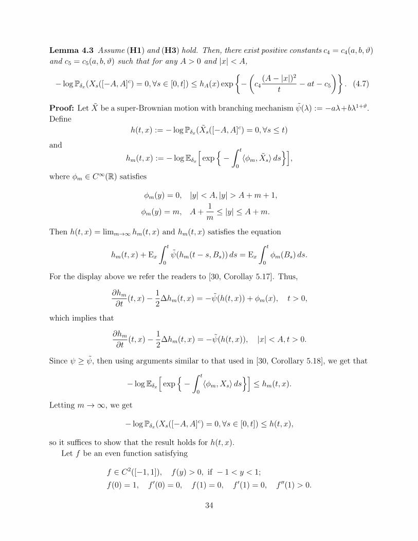
Lemma 4.3 Assume (H1) and (H3) hold. Then, there exist positive constants c4 = c4(a, b, ϑ)
and c5 = c5(a, b, ϑ) such that for any A > 0 and |x| < A,
− logPδx(Xs([−A,A]c) = 0,∀s ∈ [0, t]) ≤ hA(x) exp
{−(c4
(A− |x|)2
t− at− c5
)}. (4.7)
Proof: Let X be a super-Brownian motion with branching mechanism ψ(λ) := −aλ+bλ1+ϑ.
Define
h(t, x) := − logPδx(Xs([−A,A]c) = 0,∀s ≤ t)
and
hm(t, x) := − logEδx[
exp{−∫ t
0
〈φm, Xs〉 ds}],
where φm ∈ C∞(R) satisfies
φm(y) = 0, |y| < A, |y| > A+m+ 1,
φm(y) = m, A+1
m≤ |y| ≤ A+m.
Then h(t, x) = limm→∞ hm(t, x) and hm(t, x) satisfies the equation
hm(t, x) + Ex
∫ t
0
ψ(hm(t− s, Bs)) ds = Ex
∫ t
0
φm(Bs) ds.
For the display above we refer the readers to [30, Corollay 5.17]. Thus,
∂hm∂t
(t, x)− 1
2∆hm(t, x) = −ψ(h(t, x)) + φm(x), t > 0,
which implies that
∂hm∂t
(t, x)− 1
2∆hm(t, x) = −ψ(h(t, x)), |x| < A, t > 0.
Since ψ ≥ ψ, then using arguments similar to that used in [30, Corollary 5.18], we get that
− logEδx[
exp{−∫ t
0
〈φm, Xs〉 ds}]≤ hm(t, x).
Letting m→∞, we get
− logPδx(Xs([−A,A]c) = 0, ∀s ∈ [0, t]) ≤ h(t, x),
so it suffices to show that the result holds for h(t, x).
Let f be an even function satisfying
f ∈ C2([−1, 1]), f(y) > 0, if − 1 < y < 1;
f(0) = 1, f ′(0) = 0, f(1) = 0, f ′(1) = 0, f ′′(1) > 0.
34
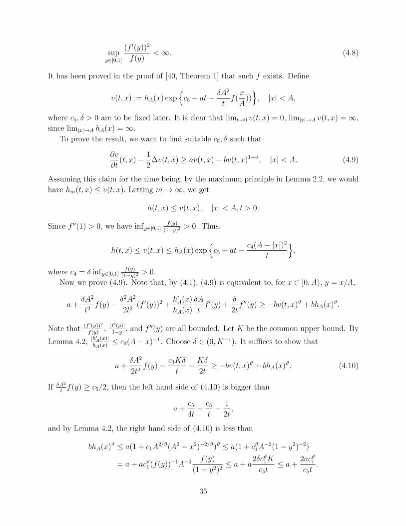
supy∈[0,1]
(f ′(y))2
f(y)<∞. (4.8)
It has been proved in the proof of [40, Theorem 1] that such f exists. Define
v(t, x) := hA(x) exp{c5 + at− δA2
tf(x
A))}, |x| < A,
where c5, δ > 0 are to be fixed later. It is clear that limt→0 v(t, x) = 0, lim|x|→A v(t, x) =∞,since lim|x|→A hA(x) =∞.
To prove the result, we want to find suitable c5, δ such that
∂v
∂t(t, x)− 1
2∆v(t, x) ≥ av(t, x)− bv(t, x)1+ϑ, |x| < A. (4.9)
Assuming this claim for the time being, by the maximum principle in Lemma 2.2, we would
have hm(t, x) ≤ v(t, x). Letting m→∞, we get
h(t, x) ≤ v(t, x), |x| < A, t > 0.
Since f ′′(1) > 0, we have infy∈[0,1]f(y)
(1−y)2> 0. Thus,
h(t, x) ≤ v(t, x) ≤ hA(x) exp{c5 + at− c4(A− |x|)2
t
},
where c4 = δ infy∈[0,1]f(y)
(1−y)2> 0.
Now we prove (4.9). Note that, by (4.1), (4.9) is equivalent to, for x ∈ [0, A), y = x/A,
a+δA2
t2f(y)− δ2A2
2t2(f ′(y))2 +
h′A(x)
hA(x)
δA
tf ′(y) +
δ
2tf ′′(y) ≥ −bv(t, x)ϑ + bhA(x)ϑ.
Note that (f ′(y))2
f(y), |f
′(y)|1−y , and f ′′(y) are all bounded. Let K be the common upper bound. By
Lemma 4.2,|h′A(x)|hA(x)
≤ c3(A− x)−1. Choose δ ∈ (0, K−1). It suffices to show that
a+δA2
2t2f(y)− c3Kδ
t− Kδ
2t≥ −bv(t, x)ϑ + bhA(x)ϑ. (4.10)
If δA2
tf(y) ≥ c5/2, then the left hand side of (4.10) is bigger than
a+c5
4t− c3
t− 1
2t,
and by Lemma 4.2, the right hand side of (4.10) is less than
bhA(x)ϑ ≤ a(1 + c1A2/ϑ(A2 − x2)−2/ϑ)ϑ ≤ a(1 + cϑ1A
−2(1− y2)−2)
= a+ acϑ1(f(y))−1A−2 f(y)
(1− y2)2≤ a+ a
2δcϑ1K
c5t≤ a+
2acϑ1c5t
.
35

Thus, when we choose c5 large enough, (4.10) is true.
If c5/2 ≥ δA2
tf(y), then the left hand side of (4.10) is bigger than
a− c3
t− 1
2t,
and the right hand side of (4.10) is less than
bhA(x)ϑ(1− eϑc5/2) ≤ −(eϑc5/2 − 1)bcϑ2A2(A2 − x2)−2
= −bcϑ2(eϑc5/2 − 1)1
f(y)A2
f(y)
(1− y)2(1 + y)2
≤ −bcϑ2δ(e
ϑc5/2 − 1)
2c5
infy∈[0,1]
f(y)
(1− y)2
1
t.
Since infy∈[0,1]f(y)
(1−y)2> 0, we can choose c5 large enough such that (4.10) is true. The proof
is now complete. 2
Proof of Lemma 3.1: It is clear that
E[
exp{−∫Rφ(y − x)Xt(dy)
},Mt ≤ x
]≥ P(‖Xt‖ = 0) > 0,
where the last inequality follows from (1.11). Thus
V (t, x) ≤ − logP(‖Xt‖ = 0) <∞,
which implies that V (t, ·) is a bounded function. For any x > 1, it follows from Lemma 4.3
that
V (t, x) ≤ − logP(Xs([−x, x]c) = 0, s ≤ t) ≤ hx(0) exp{−c4
tx2 + at+ c5}
≤ c(t)e−c4x2/t,
where c(t) is a constant which may depend on t. Thus, the desired result follows. 2
Acknowledgment: We thank the referee for helpful comments.
References
[1] E. Aıdekon. Convergence in law of the minimum of a branching random walk. Ann.Probab., 41 (2013), 1362–1426.
[2] E. Aıdekon, J. Berestycki, E. Brunet and Z. Shi. Branching Brownian motion seen fromits tip. Probab. Theory Relat. Fields, 157 (2013), 405–451.
[3] L.-P. Arguin, A. Bovier and N. Kistler. Genealogy of extremal particles of branchingBrownian motion. Comm. Pure Appl. Math. 64 (2011), 1647–1676.
36
[4] L.-P. Arguin, A. Bovier and N. Kistler. Poissonian statistics in the extremal process ofbranching Brownian motion. Ann. Appl. Probab., 22 (2012), 1693–1711.
[5] L.-P. Arguin, A. Bovier and N. Kistler. The extremal process of branching Brownianmotion. Probab. Theory Relat. Fields, 157 (2013), 535–574
[6] D. G. Aronson and H. F. Weinberger. Multidimensional nonlinear diffusion arising inpopulation genetics. Adv. in Math., 30 (1978), 33–76.
[7] A. Bovier. Gaussian processes on trees. From spin glasses to branching Brownian motion.Cambridge University Press, Cambridge, 2017.
[8] M. Bramson. Maximal displacement of branching Brownian motion. Comm. Pure Appl.Math., 31 (1978), 531–581.
[9] M. Bramson. Convergence of solutions of the Kolmogorov equation to travelling waves.Mem. Amer. Math. Soc., 44 (1983), iv+190.
[10] J. Berestycki, E. Brunet, A. Cortines and B. Mallein. Extremes of branching Ornstein-Uhlenbeck processes. Preprint. arXiv:1810.05809v1.
[11] S. Bocharov. Limiting distribution of particles near the frontier in the catalytic branch-ing Brownian motion. Acta Appl. Math., 169 (2020), 433–453.
[12] S. Bocharov and S. C. Harris. Branching Brownian motion with catalytic branching atthe origin. Acta Appl. Math., 134 (2014), 201–228.
[13] S. Bocharov and S. C. Harris. Limiting distribution of the rightmost particle in catalyticbranching Brownian motion. Electron. Commun. Probab., 21, 70(2016), 12 pp.
[14] P. Carmona and Y. Hu. The spread of a catalytic branching random walk. Ann. Inst.Henri Poincare Probab. Stat., 50 (2014), 327–351.
[15] B. Chauvin and A. Rouault. KPP equation and supercritical branching Brownian mo-tion in the subcritical speed area. Application to spatial trees. Probab. Theory RelatedFields, 80 (1988), 299–314.
[16] B. Chauvin and A. Rouault. Supercritical branching Brownian motion and K-P-P equa-tion in the critical speed-area. Math. Nachr., 149 (1990), 41–59.
[17] D. A. Dawson. Measure-Valued Markov Processes. In Ecole D’Ete de Probabilites deSaint-Flour XXI -1991. Lecture Notes in Math. 1541 1–260. Springer, Berlin, 1993.
[18] E. B. Dynkin. Superprocesses and partial differential equations. Ann. Probab., 21 (1993),1185–1262.
[19] J. Englander. Large deviations for the growth rate of the support of supercritical super-Brownian motion. Statist. Probab. Lett., 66 (2004), 449–456.
[20] R. A. Fisher. The advance of advantageous genes. Ann. Eugenics, 7(1937), 355–369.
[21] S. C. Harris. Travelling-waves for the FKPP equation via probabilistic arguments. Proc.Roy. Soc. Edinburgh Sect. A, 129 (1999), 503–517.
[22] Y. Hu and Z. Shi. Minimal position and critical martingale convergence in branchingrandom walks, and directed polymers on disordered trees. Ann. Probab., 37 (2009),742–789.
37
[23] N. Ikeda, M. Nagasawa and S. Watanabe. Markov branching processes, I. J. Math.Kyoto Univ., 8 (1968), 233–278.
[24] N. Ikeda, M. Nagasawa and S. Watanabe. Markov branching processes, II. J. Math.Kyoto Univ., 8 (1968), 365–410.
[25] N. Ikeda, M. Nagasawa and S. Watanabe. Markov branching processes, III. J. Math.Kyoto Univ., 9 (1968), 95–160.
[26] K.-S. Lau. On the nonlinear diffusion equation of Kolmogorov, Petrovsky, and Pis-counov. J. Differential Equations, 59 (1985), 44–70.
[27] S. Lalley and T. Sellke. A conditional limit theorem for the frontier of branching Brow-nian motion. Ann. Probab., 15 (1987), 1052–1061.
[28] S. Lalley and T. Sellke. Travelling waves in inhomogeneous branching Brownian motionsI. Ann. Probab., 16 (1988), 1051–1062.
[29] S. Lalley and T. Sellke. Travelling waves in inhomogeneous branching Brownian motionsII. Ann. Probab., 17 (1989), 116–127.
[30] Z. Li. Measure-Valued Branching Markov Processes. Springer, Heidelberg, 2011.
[31] O. Kallenberg. Foundations of Modern Probability. Springer-Verlag, New York, 1997.
[32] O. Kallenberg. Random Measures, Theory and Applications. Springer, Cham, 2017.
[33] A. E. Kyprianou. Travelling wave solutions to the K-P-P equation: alternatives to SimonHarris’ probabilistic analysis. Ann. Inst. Henri Poincare Probab. Stat., 40 (2004), 53–72.
[34] A. E. Kyprianou, R.-L. Liu, A. Murillo-Salas and Y.-X. Ren. Supercritical super-Brownian motion with a general branching mechanism and travelling waves. Ann. Inst.Henri Poincare Probab. Stat., 48 (2012), 661–687.
[35] A. Kolmogorov, I. Petrovskii and N. Piskounov. Etude de l’equation de la diffusionavec croissance de la quantite de la matiere at son application a un problem biologique.Moscow Univ. Math. Bull, 1 (1937), 1–25.
[36] T. Madaule. Convergence in law for the branching random walk seen from its tip. J.Theoret. Probab., 30(2017) , 27–63.
[37] P. Maillard. A note on stable point processes occurring in branching Brownian motion.Electron. Commun. Probab., 18, 5(2013), 9 pp.
[38] H. P. McKean. Application of Brownian motion to the equation of Kolmogorov-Petrovskii-Piskunov. Comm. Pure Appl. Math., 28 (1975), 323–331.
[39] Y. Nishimori and Y. Shiozawa. Limiting distributions for the maximal displacement ofbranching Brownian motions. arXiv:1903.02851, 2019.
[40] R. G. Pinsky. K-P-P-type asymptotics for nonlinear diffusion in a large ball with infiniteboundary data and on Rd with infinite initial data outside a large ball. Commun. Part.Differ. Equat., 20 (1995), 1369–1393.
[41] M. H. Protter and H. F. Weinberger. Maximum Principles in Differential Equations.Prentice-Hall, Inc., Englewood Cliffs, N.J., 1967.
38
[42] M. I. Roberts. A simple path to asymptotics for the frontier of a branching Brownianmotion. Ann. Probab., 41 (2013), 3518–3541.
[43] Y.-C. Sheu. Lifetime and compactness of range for super-Brownian motion with a gen-eral branching mechanism. Stochastic Process. Appl., 70 (1997), 129–141.
[44] Y. Shiozawa. Spread rate of branching Brownian motions. Acta Appl. Math., 155 (2018),113–150.
[45] A. I. Volpert and V. A. Volpert. Traveling Wave Solutions of Parabolic Systems. Trans-lated from the Russian manuscript by James F. Heyda. Translations of MathematicalMonographs, 140. American Mathematical Society, Providence, RI, 1994.
Yan-Xia Ren: LMAM School of Mathematical Sciences & Center for Statistical Science,Peking University, Beijing, 100871, P.R. China. Email: [email protected]
Renming Song: Department of Mathematics, University of Illinois, Urbana, IL 61801,U.S.A. Email: [email protected]
Rui Zhang: School of Mathematical Sciences & Academy for Multidisciplinary Studies,Capital Normal University, Beijing, 100048, P.R. China. Email: [email protected]
39