Extremal surfaces as bulk probes in AdS/CFT

Veronika E. Hubeny∗

Centre for Particle Theory & Department of Mathematical Sciences,

Science Laboratories, South Road, Durham DH1 3LE, United Kingdom.

March 7, 2012

DCTP-12/15

Abstract

Motivated by the need for further insight into the emergence of AdS bulk spacetime

from CFT degrees of freedom, we explore the behaviour of probes represented by spe-

cific geometric quantities in the bulk. We focus on geodesics and n-dimensional extremal

surfaces in a general static asymptotically AdS spacetime with spherical and planar sym-

metry, respectively. While our arguments do not rely on the details of the metric, we

illustrate some of our findings explicitly in spacetimes of particular interest (specifically

AdS, Schwarzschild-AdS and extreme Reissner-Nordstrom-AdS).

In case of geodesics, we find that for a fixed spatial distance between the geodesic

endpoints, spacelike geodesics at constant time can reach deepest into the bulk. We also

present a simple argument for why, in the presence of a black hole, geodesics cannot probe

past the horizon whilst anchored on the AdS boundary at both ends. The reach of an

extremal n-dimensional surface anchored on a given region depends on its dimensionality,

the shape and size of the bounding region, as well as the bulk metric. We argue that for

a fixed extent or volume of the boundary region, spherical regions give rise to the deepest

reach of the corresponding extremal surface. Moreover, for physically sensible spacetimes,

at fixed extent of the boundary region, higher-dimensional surfaces reach deeper into the

bulk. Finally, we show that in a static black hole spacetime, no extremal surface (of any

dimensionality, anchored on any region in the boundary) can ever penetrate the horizon.

∗veronika.hubeny@durham.ac.uk

arX

iv:1

203.

1044

v1 [

hep-

th]

5 M

ar 2

012

Contents

1 Introduction 1

2 Geodesic probes 6

2.1 General set-up . . . . . . . . . . . . . . . . . . . . . . . . . . . . . . . . . . . . . 8

2.2 Globally static spacetimes . . . . . . . . . . . . . . . . . . . . . . . . . . . . . . 12

2.3 Spacetimes with an event horizon . . . . . . . . . . . . . . . . . . . . . . . . . . 15

3 Extremal surface probes 21

3.1 Extremal n-surface in Poincare AdSd+1 ending on a strip . . . . . . . . . . . . . 24

3.2 Extremal n-surface in asymptotically AdSd+1 ending on a strip . . . . . . . . . . 26

3.3 Extremal n-surface in Poincare AdSd+1 enclosing a ball . . . . . . . . . . . . . . 32

3.4 Extremal n-surface in asymptotically AdSd+1 enclosing a ball . . . . . . . . . . . 33

3.5 Extremal n-surface in Poincare AdSd+1 ending on generic regions . . . . . . . . 35

4 Extremal surfaces cannot penetrate horizons 39

5 Discussion 42

1 Introduction

The gauge/gravity duality1 has been famously fruitful at revealing universal features of strongly

coupled field theories via the dual gravitational description. This has led to very successful

programs such as AdS/QCD and AdS/CMT which even bear links to present-day experiments.

On the other hand, the promise which the gauge/gravity correspondence has yet to fulfill is the

potentiality of answering long-standing questions of quantum gravity by recasting them into

non-gravitational, field-theoretic language. One prerequisite to such reformulation is a thorough

understanding of the gauge/gravity map: how do the gravitational degrees of freedom emerge

from the field theory? In particular how do the field theoretic degrees of freedom organize

themselves so as to give rise to bulk locality, at least at the classical level?

1 For definiteness we’ll consider the prototypical case of the AdS/CFT correspondence [1] which relates the

four-dimensional N = 4 Super Yang-Mills (SYM) gauge theory to a IIB string theory (or supergravity) on

asymptotically AdS5 × S5 spacetime.

1

In order to address such questions, it is useful to understand which features of the CFT

are most sensitive to the bulk geometry. For example, given a specific bulk location, what

quantities in the CFT should we examine in order to learn about the physics at the specified

location? Where on the background spacetime of the CFT are these ‘probes’ localized? As a

starting point, we want to learn how much of the bulk can given CFT observables ‘see’. More

specifically, suppose we consider some finite region B of the boundary CFT where we have

full knowledge of the relevant CFT “data”, namely we know 〈O(x) 〉, 〈O(x)O(y)〉, etc., for

all x, y ∈ B, at least for some chosen set of field theory operators O. The question we wish

to address is: what is the maximal bulk region MB for which the bulk geometry is uniquely

specified by the CFT data in B? Conversely, suppose we wish to determine the bulk metric

fully in some regionM. What is the minimal set of CFT data (in particular minimal boundary

region on which we need to specify such data) BM that will allow complete specification of the

metric in M? These are not easy questions, since bulk locality is not manifest – nor indeed

well-understood – in the dual CFT.2 On the other hand, answering them would lend us insight

into how holography encodes bulk locality, and in turn into the emergence of spacetime.

In exploring these questions, we wish to be minimalist in our assumptions about the bulk

spacetime. In particular, will not assume any field equations for the bulk, analyticity of the

metric, etc. The reason for this is the following. One might optimistically suppose that if

we can extract enough data about the bulk geometry at some spacelike slice of the bulk to

provide an initial condition for bulk evolution (and if we can liberally assume that we know

the boundary conditions at all times), then we could declare that we automatically know the

entire bulk geometry simply by evolving. In this we are effectively condensing the description

of the full spacetime to that of the initial condition, which thoroughly obscures the intricacies

of emergence of bulk time. More drastically, if the metric were analytic and we knew its exact

form in any open neighborhood, then we would automatically know it everywhere. But such

tricks miss the point of decoding the boundary-to-bulk map. Not only do they require the

knowledge of a piece of spacetime to infinite precision which is not practically possible, but

more importantly they don’t offer much intuition about how the gauge/gravity map works. To

penetrate closer to the core of the AdS/CFT mechanism it is more useful to restrict ourselves

to using only local information about the bulk geometry and try to understand which probes

see the bulk metric most directly.

Why do we elevate the bulk metric, as opposed to other bulk attributes, to be the primary

quantity of interest? There are several answers to this question. From a pragmatic standpoint,

it is the minimal set of dynamical variables which is guaranteed to exist (in more than 3 bulk

dimensions): The bulk action always contains the Einstein-Hilbert term (along with a negative

cosmological constant), and in fact this sector in isolation constitutes a consistent truncation

2 Early investigations of bulk locality from various perspectives include [2, 3, 4, 5, 6, 7] whereas more recent

developments and reviews are given in e.g. [8, 9, 10, 11, 12].

2

of the full theory. Relatedly, if we wish to extract the configuration of any other matter fields,

we may do so in addition to, but not instead of, the bulk metric, since the very notion of bulk

regions where these matter fields reside requires knowing the bulk geometry. Finally, if there

is any sort of realistic matter, as opposed to just test probes, its backreaction on the geometry

will guarantee that its presence will bear its signatures in the metric – so in that sense by

extracting the details of the bulk geometry with sufficient precision, we are detecting much of

the physics taking place in the bulk.

That said, our study deals with probes of the geometry, not physical quantities which back-

react on it. From the bulk standpoint, particularly natural constructs are various geometrical

quantities such as geodesics or higher-dimensional extremal surfaces, since their position and

geometrical attributes do not require any specification of coordinates, spacetime foliation, etc.

– they are defined in a fully covariant manner. The basic idea for using such constructs to

uncover the bulk geometry is simply the following. For given set of boundary conditions, the

location (and in turn the length/area/volume, etc.) of these quantities is determined by the

geometry. This means that they encode some aspect of the bulk geometry along their sup-

port. By comparing these quantities for nearby boundary conditions we can isolate the bulk

locations which contribute most significantly to the difference in their attributes. As indicated

below, in some circumstances one can invert this relation to extract the bulk metric explicitly.

Fortuitously, such geometric constructs find their use in the dual field theory, and in fact many

correspond to very natural and fundamental CFT probes. Here we mention a few notable

examples (for a review, see e.g. [13]).

• Geodesics: Correlators of high-dimension operators can be expressed in the WKB ap-

proximation heuristically as

〈O(x)O(y)〉 ∼ e−mL(x,y) (1.1)

where m is the mass of the bulk field corresponding to O and L(x, y) is a regularized

proper length along a spacelike geodesic connecting x and y. Since such geodesic passes

through the bulk, this correlator is sensitive to the corresponding region of the bulk

geometry. This was used to identify the CFT signature of the black hole singularity

[14, 15], building on prior work of [16, 17, 18], by considering the insertion points x

and y on two disconnected boundaries corresponding to the two asymptotic regions of

an eternal black hole.3 However, the impressive amount of information extractible from

these correlators comes with a cost: since the insertion points are not located on the

3 In fact as later demonstrated in [19], by examining the detailed analytic structure of such correlation

functions, one can tell apart spacetimes with and without horizons, and even distinguish such subtle differences

as the fuzzball picture of the black hole [20, 21] and a genuine eternal black hole geometry. Indeed, one can use

similar correlators to discern even more subtle signals of the bulk geometry from behind the black hole horizon,

such as explored in [22] to investigate aspects of inflationary cosmology within AdS/CFT.

3

same boundary, accessing this information as genuine signal in the CFT requires analytic

continuation. That in turn imposes unwanted restriction on the spacetime.

This shortcoming is avoided in the framework of [23], which considers the structure of sin-

gularities of generic Lorentzian correlators, observing that these correlators exhibit light-

cone singularities when the operator insertion points are connected by a null geodesic.

This geodesic can lie along the boundary (which gives rise to the familiar light cone singu-

larity in the field theory), or it can traverse the bulk, emerging within4 the boundary light

cone; the latter give rise to the bulk-cone singularities. The structure of these singularities

was recently examined by [25] (following [26, 27]) in context of moving mirror in AdS. As

pointed out in [23], bulk-cone singularities can be used to extract part of the spacetime

geometry, even including the location of the bulk event horizon formation in a collapse

geometry. This was subsequently used in [28, 29] for recovering the metric within a sim-

ple class of static spherically symmetric spacetimes, by numerical and analytical means

respectively.

• Extremal surfaces: The expectation value of a Wilson-Maldecena loop is related to the

area of two-dimensional extremal surface describing a string world-sheet ending on the

corresponding contour in the boundary of AdS [30, 31]. Similarly, the entanglement

entropy [32],[33] associated to a given region A in the boundary is related to the area of

a co-dimension 2 extremal5 surface ending on ∂A. This was first developed by [36, 37]

for static configurations and later generalized to time-dependent situations by [34], which

emphasized its use in extracting bulk geometries and demonstrated how this proposal may

be used to understand the time evolution of entanglement entropy in a time varying QFT

state dual to a collapsing black hole background. The analysis of thermalization (serving

as a toy model of “quantum quench”) initiated in [34] was recently extended by [38, 39]

in 3-dimensional bulk, in [40] for 4 dimensions, and [41, 42] in 3,4 and 5 dimensions, the

latter having used entanglement entropy as well as equal time correlators and Wilson

loop expectation values. (See also [43, 44] for other recent explorations of holographic

entanglement entropy as a probe in different contexts.)

One might naively wonder why we don’t simply use the expectation value of the boundary

stress tensor to extract the bulk metric, since after all it is the boundary stress tensor which

couples to the bulk metric. Indeed, several previous approaches utilized this substantially. In

4 As proved by [24], in a certain wide class of spacetimes with timelike conformal boundary, any fastest null

geodesic connecting two points on the boundary must lie entirely within the boundary. The vacuum state of

the CFT plays a distinguished role in this context, as all null geodesics through pure AdS bulk take the same

time to reach the antipodal point as the boundary null geodesics.5 As argued in [34], such extremal surface is in fact related to light-sheet constructions of the covariant

entropy bound [35] in the bulk spacetime. Note that in 2+1 bulk dimensions, the bulk duals of equal-time

correlators, Wilson loops, and entanglement entropy probes all degenerate to constant-time spacelike geodesics.

4

the holographic renormalization group scheme of [45], one can reconstruct the asymptotic be-

haviour of the bulk geometry using Fefferman-Graham expansion around the boundary. This

expansion however is not guaranteed to converge deep in the bulk, and in fact would gener-

ically lead to singular geometries. In the fluid/gravity correspondence [46] the problem of

singularities is avoided by working in the long-wavelength regime, where the boundary stress

tensor prescribes the bulk geometry down to well inside the bulk event horizon. This may then

appear attractively good probe of the geometry, but it comes at the cost of disallowing any

sharp variations in the bulk geometry; in a sense, we can ‘probe’ so deep into the bulk mainly

because there’s not much happening in the transverse directions, so the main variation (in the

radial direction) is very similar to the exact solution of a static black hole we know already. So

neither of these methods would be able to discern a localized deformation in the geometry, say,

somewhere in the vicinity of the event horizon.

A more pedestrian way to state the shortcoming of the stress tensor expectation value is

that it only knows about the asymptotic fall-off of the bulk metric. In fact, it is trivial to

construct examples with matter which have the same boundary stress tensor but drastically

different bulk metric. One such example is a spherically symmetric distribution of matter. The

asymptotic metric fall-off only knows about the total ADM mass, whereas the bulk geometry

is of course sensitive to the radial density profile and time dependence of this matter. This

shortcoming is of course avoided if we don’t restrict ourselves merely to the expectation values

of the stress tensor, but are allowed to consider its higher point functions as well. However, once

we allow this level of complexity, we might as well consider n-point functions of more general

operators without worrying about the tensor structure, as well as more non-local observables.

Therefore we will focus on CFT quantities such as correlators, Wilson loop expectation

values, and entanglement entropy, which provide examples of our probes, i.e. “data” that we’ll

assume we have access to in some region of the CFT. Rather than furthering the program

of using these to extract the bulk geometry, we wish explore the more general question of

which of these is the best-suited for extracting the bulk geometry. As mentioned above, for

asking matter-of-principle questions such as what is the best CFT probe of bulk geometry, it

is convenient to separate this issue from the field equations. We will therefore refrain from

imposing Einstein’s equations. Instead, we consider any physically sensible geometry (which

would be supported by some physical matter), and ask what is the most economical way to

decode parts of this geometry from the boundary data. On the other hand, in order to make

progress, we will focus on static and spherically or translationally symmetric geometries. The

expectation is that these cases, albeit highly symmetric, are sufficiently indicative of the general

case, in terms of elucidating which CFT probe is the best-suited to probing the bulk geometry.

Of special interest in our considerations will be causally nontrivial spacetimes corresponding

to a black hole in AdS. It is clear by causality that no timelike or null curve in the bulk

can probe inside the black hole horizon while being anchored to the AdS boundary at both

5

ends. No such causal obstruction applies to spacelike curves of course, however the story is

more interesting for spacelike geodesics or higher-dimensional extremal surfaces. We will first

show that in fact in static spherically symmetric spacetimes spacelike geodesics likewise cannot

penetrate the horizon, and subsequently generalize this statement to a much larger family of

higher-dimensional extremal surfaces anchored on the boundary. As we remark below, this is no

longer true in general for time-evolving spacetimes; indeed it is easy to find counter-examples,

such as given in [47].

The structure of this paper is as follows. In Section 2 we focus on geodesic probes of static,

spherically symmetric, asymptotically AdS spacetimes. Apart from the result mentioned above

that these cannot penetrate black holes, we argue that the best-suited geodesics for probing

deepest into the bulk are the spacelike ones localized at constant time. Motivated by this

observation, we go on to consider extremal surfaces anchored on the boundary at constant time.6

For simplicity, we also switch from global AdS to Poincare AdS, namely consider extremal

surfaces in general static asymptotically AdS spacetimes which are translationally invariant

in the boundary directions. In Section 3 we examine these surfaces anchored on variously-

shaped boundary regions of various dimensionalities, exploring how these attributes affect the

depth to which such surfaces can reach in the bulk. We also consider the effect that spacetime

deformations have on this reach. We conclude by presenting an argument that out of all possible

shapes with fixed area or extent, spherical regions allow for the greatest reach. Section 4 focuses

on spacetimes with horizons, demonstrating that extremal surfaces of any dimensionality, and

anchored on arbitrarily shaped region in the boundary, cannot penetrate event horizon in

our general class of spacetimes. Further discussion and summary of the main results appears

in Section 5. A preview of some of these results were given in [13], and some related results

appeared in e.g. [23, 37, 34]; however we have attempted to keep the presentation self-contained

and pedagogical.

2 Geodesic probes

In this section we consider CFT probes related to bulk geodesics anchored on the AdS boundary

at both endpoints. We will refer to such geodesics as probe geodesics, since they can be more

directly associated to a natural CFT probe. Our main concern is how sensitive are these

probe geodesics to the geometry of a given bulk spacetime. For simplicity, we will restrict our

considerations to asymptotically (globally) AdS, static, spherically symmetric bulk spacetimes.

6 These are often referred to as “minimal surfaces” in the literature; however since we are working in

Lorentzian spacetime where the area of a spacelike surface can be decreased by deforming it in the timelike

direction, we will maintain the terminology “extremal”.

6

By a suitable choice of coordinates we can write the line element as

ds2 = −f(r) dt2 + h(r) dr2 + r2 dΩ2 (2.1)

where f and h are a-priori arbitrary7 radial functions with the large-r behaviour determined

by the AdS asymptotics, namely f(r) ∼ 1h(r)∼ r2 + 1 as r →∞, and we are for now keeping

the spacetime dimension d + 1 arbitrary. Note that in the above expression we have fixed the

AdS radius to unity, tantamount to measuring all distances in AdS units.

We want to ask the following questions:

• How much of the bulk is accessible to the set of all probe geodesics? For spherically

symmetric spacetimes (2.1), this will be characterized by the minimal radius r∗ to which

probe geodesics can reach. For pure AdS and small deformations thereof, the answer is of

course the full spacetime so r∗ = 0; however, there exist physically relevant spacetimes,

such as ones with a black hole, where some part of the bulk cannot be reached by geodesics

with both endpoints anchored on the (same) boundary.

• In the latter set of cases where some part of the bulk remains inaccessible, which probe

geodesics can reach the deepest? Since all geodesics in (2.1) can be characterized by

energy E and angular momentum L, as well as the discrete parameter κ distinguishing

null, spacelike, and timelike ones, this question boils down to finding the optimal E, L,

and κ which minimize the corresponding r∗.

• A further refined question is, for some restricted region on the boundary from which we

allow the probe geodesics to emanate, what part of the bulk is accessible?

• It is also of interest to know what is the (regularized) proper length of a given probe

geodesic? We expect that the larger this quantity is, the harder it would be to extract

from the corresponding CFT probe. On the other hand, shorter-length geodesics typically

reach less deep into the bulk, so they carry less information about the geometry.

To preview the main results, we will see that in any spacetime of the form (2.1):

1. For given E and L, spacelike geodesics necessarily probe deeper than null ones.

2. For restricted angular separation of the endpoints, the spacelike geodesic which reaches the

deepest is the one moving in constant-time slice, with smallest allowed angular momentum

consistent with the restriction on the endpoints.

7 Ultimately, their functional dependence will be constrained by the Einstein’s equations and boundary

conditions; but as motivated in the Introduction, we will consider arbitrary spacetimes, which are not necessarily

solutions to any specified field equations.

7

3. When the geometry contains a black hole, probe geodesics cannot reach past the horizon.

However, by suitable adjusting of the parameters we can find a probe geodesic which

reaches arbitrarily close to the horizon.

4. Nevertheless, if we impose an upper bound on the angular separation of the endpoints

or the regularized proper distance of such a probe geodesic, the restricted probe geodesic

only reaches to some finite distance from the horizon. In practice, this is not too drastic

a constraint, and the near-horizon region remains accessible for sensible restrictions.

5. Null probe geodesics, on the other hand, can only penetrate to the unstable circular orbit

around the black hole, which is typically some O(1) distance from the horizon.

The remainder of this section consists of a pedagogical derivation of these results. In Section

2.1 we describe the geodesic in terms of 1-D motion in an effective potential for arbitrary

spacetime of the form (2.1), focusing on the minimal radius r∗ reached by such a geodesic, its

endpoints, and the regularized proper length. To make our discussion more specific, we then

separate the set of possibilities into two classes: globally static spacetimes (which are causally

trivial), addressed in Section 2.2, and spacetimes with an event horizon, addressed in Section

2.3, where we give the general proof that probe geodesics cannot reach past the horizon. For

illustrative purposes, we include the particular example of pure AdS in Section 2.2 and three

black hole spacetimes (BTZ, Schwarzschild-AdS5, and extremal Reissner-Nordstrom-AdS5) in

Section 2.3.

2.1 General set-up

Let us consider a general geodesic in a static spherically symmetric spacetime (2.1). Using

spherical symmetry, we can fix angular coordinates such that a given geodesic remains confined

to the equator of the Sd−1. Denoting the azimuthal angle ϕ, we can then write the tangent

vector along this geodesic as

pa = t ∂at + r ∂ar + ϕ ∂aϕ (2.2)

where ˙≡ ddλ

with λ denoting the affine parameter along the geodesic. Using the usual constants

of motion induced by the Killing fields ∂at and ∂aϕ, namely the energy E ≡ −pa ∂at = f(r) t and

angular momentum L ≡ pa ∂aϕ = r2 ϕ, and the norm of the tangent vector κ ≡ pa p

a (fixed to

κ = +1, 0,−1 for spacelike, null, and timelike geodesics, respectively), we can recast the radial

geodesic equation in terms of a 1-d motion in an effective potential Veff ,

r2 + Veff(r) = 0 , Veff(r) =1

h(r)

[−κ− E2

f(r)+L2

r2

]. (2.3)

Since classically defined geodesic motion requires r2 ≥ 0, the condition for such a geodesic to

reach the boundary is then simply Veff(r →∞) < 0, and the deepest into the bulk (i.e. smallest

8

r) that such a geodesic reaches, denoted r∗, is given by the largest root of Veff(r). The main

goal of this section is to study the behaviour of r∗.

Using the AdS asymptotics, we can immediately see that at large r, for non-null geodesics

Veff is dominated by Veff ∼ −κ r2, so timelike geodesics (κ = −1) cannot reach the boundary

for any finite value of E and L. On the other hand, all spacelike geodesics (in this asymptotic

region) necessarily reach the boundary for any value of E and L. For null geodesics, since κ = 0,

by constant rescaling the affine parameter we can fix E = 1 and parametrize the geodesic by a

single parameter ` ≡ L/E, so that at large r, Veff ∼ `2 − 1. This means that in order for null

geodesics to reach the boundary,8 we need to take `2 < 1 (the limiting value of ` = ±1 would

correspond to the null geodesic staying on the boundary, i.e. r∗ = ∞). Finally, note that the

high-energy limit of a spacelike geodesic, E →∞ with ` = L/E fixed, corresponds to the null

geodesic with angular momentum ` and infinitely rescaled affine parameter.9 We will therefore

only consider spacelike geodesics (κ = 1 with arbitrary E and L) and null geodesics (κ = 0

with E2 < L2 or equivalently `2 < 1). In order to capture the behaviour of both spacelike and

null geodesics, we will keep describing the null ones in terms of the redundant notation of E

and L, and simply set κ = 0 in the resulting expressions.

Reach of spacelike versus null geodesics: We first give a very simple argument why

certain spacelike geodesics can reach deeper into the bulk (i.e. have smaller r∗) than given null

geodesics. The argument uses the assumption that h(r) and f(r) are positive in the region of

interest, r∗ ≤ r < ∞, whose proof we postpone till Section 2.3. Consider any null geodesic,

specified by `. This is described by an effective potential (2.3) with κ = 0 and L = `E for any

E > 0. Denote its largest root by r(κ=0)∗ . Now, a spacelike geodesic with the same E and L

will have its effective potential lowered everywhere by 1h(r)

> 0. This means that in particular

at r(κ=0)∗ , the effective potential for this spacelike geodesic will still be negative, and therefore

its largest root r(κ=1)∗ will have to occur at smaller value of r, i.e. r

(κ=1)∗ < r

(κ=0)∗ .

We emphasize that this argument holds for general spacetimes, as long as h(r) > 0 for

r ≥ r(κ=0)∗ . This is automatically satisfied when the spacetime is globally static, so that h(r) > 0

for all r ≥ 0. As discussed in Section 2.2, in such a case, both sets of geodesics can probe to

arbitrarily small radii r∗ simply by choosing the angular momentum to be small enough. In

8 Depending on the spacetime, there may or may not exist null geodesics with `2 > 1: in pure AdS, it is easy

to see that `2 > 1 null geodesics simply do not exist, since Veff(r) > `2−1r2 > 0 for `2 > 1. On the other hand, in

a black hole geometry, null geodesics can exist for arbitrary `, but for `2 > 1 they cannot reach the boundary.

In fact, for very large `2, they cannot emerge far from the vicinity of the horizon: rmax − r+ ∼ 1/`2.9 Note that one has to be careful about order of limits, as illustrated by the following example: consider

spacelike geodesic with say L = 2E and take the limit E → ∞ with L/E fixed. This is a null geodesic with

` = 2 which therefore cannot reach the boundary, yet all spacelike geodesics in this family were anchored on

the boundary. (However, r∗ →∞ as E →∞.)

9

a causally non-trivial case, h(r) may be negative, but we will argue Section 2.3 that for any

probe geodesic r∗ is bounded from below in such a way that the h(r) < 0 region can never be

reached.

It is also easy to see from (2.3) the effects of shifting E and L whilst keeping the other

parameters fixed:

• If we increase L2 while keeping E fixed, Veff increases at all r where h(r) > 0, so r∗likewise increases. This is to be expected since there is greater centrifugal barrier.

• On the other hand, as E2 increases with L fixed, Veff decreases at all r, so r∗ decreases.

• However, as E2 increases with ` = L/E fixed, Veff increases in the vicinity of the turning

point, so r∗ increases.

We can see the last statement more clearly by writing (2.3) for the spacelike case as

V(κ=1)

eff (r) =1

h(r)

(−1 + E2

[− 1

f(r)+`2

r2

]), (2.4)

so that r(κ=1)∗ occurs at a value of r for which

[− 1f(r)

+ `2

r2

]= 1

E2 , which is positive. This means

that the coefficient of E2 in V(κ=1)

eff (r) is some function of r, which is positive at r = r∗. Hence

if we lower E2, the effective potential will decrease at the original turning point r = r∗, which

in particular means that the new10 turning point will shift to lower value of r. This implies

that to minimize r(κ=1)∗ at fixed `, we need to minimize E2, namely consider the case E = 0.

We can in fact now figure out what the minimal radius is. As long as h(r) > 0 for all r,

we can probe the full spacetime. Indeed, as is clear from (2.3), setting E = 0 and κ = 1, we

immediately see that r∗ = |L|, which can be taken to r = 0 when L = 0. As we will show in

Section 2.3, if there is an event horizon at some r = r+, then we can probe down to it.

Geodesic endpoints and proper length: Having addressed part of our first two questions,

namely how much of the bulk is accessible to probe geodesics and which ones probe deepest,

we now turn to the remaining two questions, which concern the endpoints and proper length

of the geodesic. In particular, suppose we have only a finite region in the CFT at our disposal,

within which we can anchor our geodesic endpoints. We would then be interested in finding

10 Note that although the term in square brackets can take both positive and negative values depending on

r, we can see that decreasing E2 cannot suddenly introduce new larger roots of Veff , essentially by running the

previous argument backwards: raising E2 increases the value of Veff near all its roots, but since Veff(r =∞) < 0,

this operation would increase r∗ rather than getting rid of it entirely.

10

the ‘optimal’ probe geodesic within this restricted set of geodesics. To that end, we need to

specify the endpoints of a general probe geodesic.

Recall that we wish to focus on probe geodesics whose endpoints at λ = ±∞ are anchored on

the boundary r =∞. Due to the time-translational and rotational symmetry of the spacetime

(2.1), the relevant data on the boundary are the temporal and angular distances between the

two geodesic endpoints,

∆t ≡ 2

∫ ∞r∗

E

f(r)g(r) dr and ∆ϕ ≡ 2

∫ ∞r∗

L

r2g(r) dr , (2.5)

where we have simplified the notation somewhat by defining

g(r) ≡√

h(r)

κ+ E2

f(r)− L2

r2

=1√−Veff(r)

=1

|r(r)|. (2.6)

Note that in each case both the integrand and the lower limit of integration r∗ depend on the

specific geodesic, characterized by the constants of motion E and L, as well as on the spacetime,

described by the functions f(r) and h(r). At large r the integrands of (2.5) are proportional to

1/r3 for spacelike geodesics and 1/r2 for null geodesics, so that at the upper limit the integrals

converge. Moreover, it is easy to see that in the absence of unstable circular orbits, the integrals

(2.5) also converge at the lower limit. In particular, in the general case of V ′eff(r∗) 6= 0, the we

can write Veff(r) ≈ V ′eff(r∗) (r − r∗), so that using g(r) = 1√−Veff(r)

we have the integrands near

r ≈ r∗ scale with 1√r−r∗ .

For null geodesics the requirement that Veff(r) < 0 for all r > r∗ implies that L2

r2 <E2

f(r), so

by comparing the integrands in (2.5), we can easily see that

∆t ≥ `∆ϕ . (2.7)

This is however already guaranteed by the stronger bound ∆t ≥ ∆ϕ implied by a theorem of

Gao & Wald [24] which states that (subject to certain energy conditions) one can’t propagate

faster through the bulk than along the boundary. Slightly stronger conditions can be obtained

by considering the variation of the geodesic endpoints under varying the parameters. For

example, by varying the angular momentum ` of null geodesics in any geometry, we obtain

δ∆t

δ`= `

δ∆ϕ

δ`, (2.8)

and an analogous relation may be obtained for spacelike geodesics.

Finally, let us briefly turn to the proper length along a spacelike geodesic. Since such a

geodesic reaches the boundary, its proper length is by definition infinite; however we can easily

11

regulate it. Simply imposing a large-radius cutoff at r = R, the proper length along the part

of the geodesic with r ≤ R is given by

LR = 2

∫ R

r∗

g(r) dr . (2.9)

Following standard procedure, we then define the regularized proper length Lreg by a back-

ground subtraction method as the large-R limit of the difference between Lreg in the spacetime

of interest and Lreg for the geodesic in pure AdS with the same endpoints. In practice, this

amounts to stripping off the R-dependent part from LR.

To make more definite statements about the behaviour of r∗, ∆ϕ, ∆t, and Lreg for various

spacetimes and parameters of a probe geodesic, let us now consider the case of spacetimes with

and without horizons separately. We start with the simpler case of causally trivial spacetimes

in Section 2.2, and then turn to the more interesting black hole spacetimes in Section 2.3.

2.2 Globally static spacetimes

When the spacetime (2.1) is globally static, the Killing vector ∂at is timelike everywhere, so

f(r) > 0 for all r ≥ 0, and Lorentzian signature then simultaneously forces h(r) > 0 for all

r ≥ 0. For convenience, we will consider the cases of radial geodesics with L = 0 and non-radial

geodesics with L 6= 0 separately.

L = 0 case: Let us first consider the special case of radial geodesics. For L = 0, the effective

potential (2.3) is manifestly negative everywhere, so the geodesic continues all the way from

the boundary to the origin. The origin r = 0 is a regular point, so the geodesic simply passes

through, and continues back to r =∞ on the antipodal point of the sphere. Since the spacetime

is globally static, it is causally trivial, so both geodesic endpoints lie on the same boundary.

The angular difference between the endpoints is simply ∆ϕ = π, while the time delay depends

on the energy and the spacetime. For null geodesics, the energy cancels out (as it must), and

the time delay is simply given by

∆tκ=0,L=0 = 2

∫ ∞0

√h(r)

f(r)dr , (2.10)

whereas for spacelike geodesics (2.5) gives

∆tκ=1,L=0 = 2

∫ ∞0

√h(r)

f(r)

√1

1 + f(r)E2

dr . (2.11)

Note that as E → ∞ in the spacelike geodesic case, we recover the null geodesic result. It

is now easy to compare ∆t between the spacelike and null case, for arbitrary globally static

12

spacetimes. In particular, since the integrand in (2.11) is always less than the integrand in

(2.10), we see that ∆tκ=1,L=0 < ∆tκ=0,L=0, as we would expect. Moreover, within the family

of spacelike geodesics, ∆tκ=1,L=0 decreases with E; for E = 0, ∆tκ=1,L=0,E=0 = 0, as expected.

This is intuitively obvious, since faster geodesics traveling the same spatial trajectory arrive in

shorter time.

L 6= 0 case: We now turn to the more general case of L 6= 0. Since h(r) > 0 for all r ≥ 0, in

looking for solution of Veff(r∗) = 0, we can ignore the overall 1h(r)

factor in (2.3). The minimal

radius r∗ can then be found by solving

− 1− E2

f(r)+L2

r2= 0 at r = r∗ . (2.12)

Since L 6= 0, there must always exist a solution r∗ > 0 since at small r the third term on the

LHS of (2.12) dominates, making the LHS large and positive, whereas at large r the dominant

first terms makes the LHS negative. It is easy to see that as we tune L for given E, r∗ ranges

over all positive values. In particular as f varies between f(r = 0) = f0 and f(r → ∞) ∼ r2,

we have the small-L and large-L regime solutions:

r∗ ≈|L|√

1 + E2

f0

as L→ 0 and r∗ ≈ |L| as L→∞ . (2.13)

Unfortunately, in this case it is no longer as straightforward to compare ∆t and ∆ϕ between

null and spacelike geodesics, unlike in the L = 0 case. This is because both the integrand, and

the lower limit of integration, in (2.5) is larger for a null geodesic case than for the spacelike

geodesic with same E and L, so the overall integral depends more sensitively on the details.

Explicit expressions for pure AdS: To get better intuition, let us consider the simplest

case of pure AdS, where the relevant expressions can be obtained in closed form. We have

f(r) = h(r)−1 = r2 + 1, for which case the effective potential for null and spacelike geodesics

respectively simplifies to

V(κ=0)

eff (r) = L2 − E2 +L2

r2and V

(κ=1)eff (r) = −r2 + (L2 − E2 − 1) +

L2

r2. (2.14)

We can easily find the minimal radius reached for any given geodesic. For null geodesics,

r(κ=0)∗ =

√L2

E2 − L2=

|`|√1− `2

, (2.15)

whereas for spacelike geodesics,

r(κ=1)∗ =

√1

2

[−(E2 − L2 + 1) +

√(E2 − L2 + 1)2 + 4L2

]. (2.16)

13

For a spacelike geodesic with E = 0, as in any globally static spacetime, the minimal radius

must be at

r(κ=1,E=0)∗ = |L| , (2.17)

which is indeed easy to verify directly from (2.16). In fact, the full radial trajectory of such

E = 0 geodesic, with r∗ occurring at ϕ = 0 can be written in a very simple closed-form

expression as

r2(ϕ) =L2

cos2 ϕ− L2 sin2 ϕ. (2.18)

From the form of (2.16), we can easily confirm that at fixed L, increasing E has the effect of

lowering r(κ=1)∗ . On the other hand, at fixed ` = L/E, increasing E increases r

(κ=1)∗ .

Let us now examine the relation between r∗ and (∆t,∆ϕ). By direct integration of (2.5),

we find that for a spacelike geodesic with arbitrary E and L,

∆ϕ =π

2+ sin−1

[E2 − L2 + 1√

(E2 − L2 + 1)2 + 4L2

](2.19)

and

∆t =π

2+ sin−1

[E2 − L2 − 1√

(E2 − L2 − 1)2 + 4E2

]. (2.20)

As an aside, we note that E cot ∆t− L cot ∆ϕ = 1 for E,L > 0. In the special case of E = 0

spacelike geodesics, we find ∆t = 0 and ∆ϕ is related to the angular momentum as

∆ϕ =π

2+ sin−1 1− L2

1 + L2= 2 cot−1 |L| , (2.21)

whereas for null geodesics, we have ∆t = ∆ϕ = π independently of `.

We can also easily confirm that for fixed ∆ϕ (leaving ∆t arbitrary), r∗ is minimized at

E = 0 and grows monotonically with E2. This implies that if one has access to CFT data only

in a certain region ∆ϕ, we can probe more of the bulk geometry with spacelike geodesics than

with null geodesics.

For future reference, the regularized proper length along a spacelike geodesic, given by (2.9)

with the universal divergent piece ln(4R2) stripped off, is

Lreg = − ln√

(E2 − L2 + 1)2 + 4L2 . (2.22)

For E = 0 geodesics, this simplifies to Lreg = − ln (1 + L2), which vanishes for radial geodesics.

For fixed L, we see that the geodesic which minimizes r∗, namely the constant-time one with

E = 0, in fact maximizes its length Lreg. The same conclusion holds for fixed ∆ϕ.

14

2.3 Spacetimes with an event horizon

We now consider asymptotically-AdS spacetimes with a spherical black hole, i.e. spacetimes

which are spherically symmetric and static, but not globally static. The event horizon is a

Killing horizon where the Killing field ∂at has zero norm. At this radial position, which we’ll

denote by r+, f(r+) = 0. Although the static coordinates as written in (2.1) are singular on

the horizon, we can easily pass to regular (e.g. ingoing Eddington) coordinates by defining

v = t+ r∗ , where dr∗ =

√h(r)

f(r)dr (2.23)

upon which the line element (2.1) becomes

ds2 = −f(r) dv2 + 2√f(r)h(r) dv dr + r2 dΩ2 (2.24)

and the conserved energy along a geodesic is E = f(r) v−√f(r)h(r) r. The effective potential

for geodesics of course still retains the same form as in (2.3), namely

Veff(r) =1

h(r)

[−κ− E2

f(r)+L2

r2

]. (2.25)

Let us now consider the general properties of Veff(r), in particular the position of r∗, which

depends both on the spacetime specification f(r) and h(r), and on the geodesic (i.e. κ, E,

and L). Our present strategy will be the following: given a generic spacetime of the kind

described above, we wish to explore what kinds of geodesics are possible on this spacetime.

In particular, what is the minimum r∗ achievable by any probe geodesic (i.e. one with both

endpoints anchored to the boundary), and for what E,L, κ is it realized?

On the horizon r = r+ where f(r+) = 0, we need f(r+)h(r+) > 0 to keep the metric well-

defined and Lorentzian. This means that the only term which survives in the effective potential

at that point is

Veff(r+) = − E2

f(r+)h(r+)< 0 ∀ E 6= 0 . (2.26)

Let us for now assume that E > 0 (this simultaneously covers the cases of E < 0 by flipping

the time, and we’ll return to the special case of E = 0 later). Then there are two qualitatively

distinct possibilities for the behaviour of Veff :

1. Veff(r) < 0 for all r > r+. Then the geodesic crosses the horizon and either there is a

turning point inside the horizon at r∗ < r+, or the geodesic continues to r = 0. In case

of singularity at r = 0, the geodesic ends there; otherwise r∗ = 0 and the geodesic merely

passes through a smooth origin.

15

?

HaL HbL HcL HdL HeL

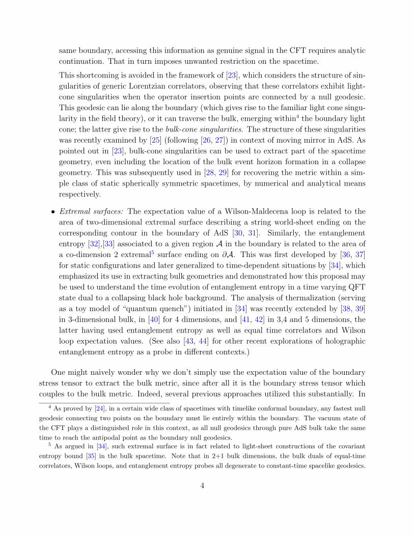
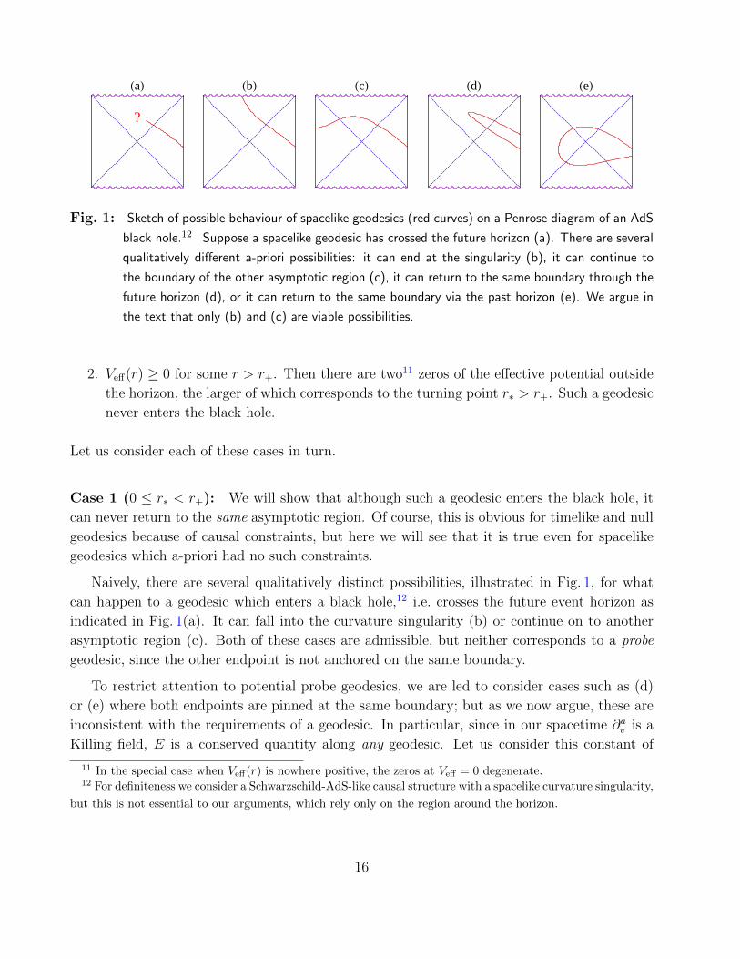
Fig. 1: Sketch of possible behaviour of spacelike geodesics (red curves) on a Penrose diagram of an AdS

black hole.12 Suppose a spacelike geodesic has crossed the future horizon (a). There are several

qualitatively different a-priori possibilities: it can end at the singularity (b), it can continue to

the boundary of the other asymptotic region (c), it can return to the same boundary through the

future horizon (d), or it can return to the same boundary via the past horizon (e). We argue in

the text that only (b) and (c) are viable possibilities.

2. Veff(r) ≥ 0 for some r > r+. Then there are two11 zeros of the effective potential outside

the horizon, the larger of which corresponds to the turning point r∗ > r+. Such a geodesic

never enters the black hole.

Let us consider each of these cases in turn.

Case 1 (0 ≤ r∗ < r+): We will show that although such a geodesic enters the black hole, it

can never return to the same asymptotic region. Of course, this is obvious for timelike and null

geodesics because of causal constraints, but here we will see that it is true even for spacelike

geodesics which a-priori had no such constraints.

Naively, there are several qualitatively distinct possibilities, illustrated in Fig. 1, for what

can happen to a geodesic which enters a black hole,12 i.e. crosses the future event horizon as

indicated in Fig. 1(a). It can fall into the curvature singularity (b) or continue on to another

asymptotic region (c). Both of these cases are admissible, but neither corresponds to a probe

geodesic, since the other endpoint is not anchored on the same boundary.

To restrict attention to potential probe geodesics, we are led to consider cases such as (d)

or (e) where both endpoints are pinned at the same boundary; but as we now argue, these are

inconsistent with the requirements of a geodesic. In particular, since in our spacetime ∂av is a

Killing field, E is a conserved quantity along any geodesic. Let us consider this constant of

11 In the special case when Veff(r) is nowhere positive, the zeros at Veff = 0 degenerate.12 For definiteness we consider a Schwarzschild-AdS-like causal structure with a spacelike curvature singularity,

but this is not essential to our arguments, which rely only on the region around the horizon.

16

motion E at the future horizon:

E =[f(r) v −

√f(r)h(r) r

]r+

= −√f(r+)h(r+) r > 0 (2.27)

where the second equality holds since f vanishes while v remains finite and the inequality holds

because when the geodesic enters the horizon, r decreases, so r < 0. But the constancy of E

then precludes the geodesic from exiting back out of the future horizon, which would require

r(r+) > 0, and therefore E < 0. This simple argument implies that case (d) is disallowed, i.e.,

no geodesic can exit the same future horizon it enters.

One might try to circumvent the above argument by letting the geodesic come back out

through the past horizon instead, as indicated in (e), since there (2.27) no longer holds as

v → −∞ at the past horizon. However, this fails for a simpler reason, namely that there

would then have to be another turning point for some r > r+, which contradicts our starting

assumption that the geodesic reached the horizon all the way from infinity. Thus case (e) is

disallowed as well.

Thus, we have learned that no geodesic with turning point inside the horizon can have both

its endpoints anchored to the same boundary. In other words, no probe geodesic can reach past

the horizon. Thus from the point of view of asking how deep into the bulk can probe geodesics

reach, only Case 2 is relevant. In particular, we can now WLOG assume that h(r) > 0 and

f(r) > 0 for all r in the region of interest, i.e. in the entire bulk region accessible to probe

geodesics.

Case 2 (r∗ > r+): The bounce occurs outside the horizon, so it is evident that such a geodesic

cannot probe past the horizon. It is nevertheless interesting to ask how close to the horizon can

it approach; in particular, for a given geometry, which types of geodesics have turning point as

close as possible to the horizon?

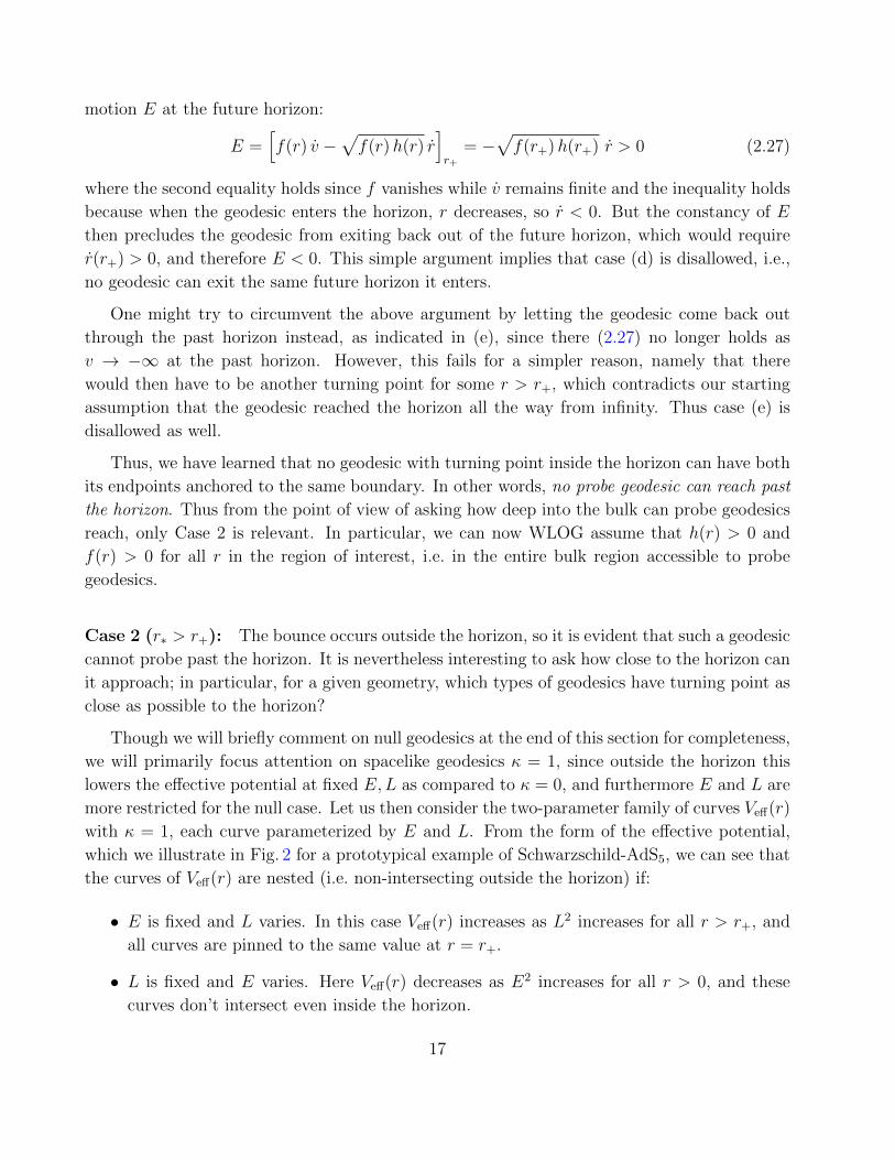
Though we will briefly comment on null geodesics at the end of this section for completeness,

we will primarily focus attention on spacelike geodesics κ = 1, since outside the horizon this

lowers the effective potential at fixed E,L as compared to κ = 0, and furthermore E and L are

more restricted for the null case. Let us then consider the two-parameter family of curves Veff(r)

with κ = 1, each curve parameterized by E and L. From the form of the effective potential,

which we illustrate in Fig. 2 for a prototypical example of Schwarzschild-AdS5, we can see that

the curves of Veff(r) are nested (i.e. non-intersecting outside the horizon) if:

• E is fixed and L varies. In this case Veff(r) increases as L2 increases for all r > r+, and

all curves are pinned to the same value at r = r+.

• L is fixed and E varies. Here Veff(r) decreases as E2 increases for all r > 0, and these

curves don’t intersect even inside the horizon.

17

r+

r

Veff

E=2

r+

r

Veff

L=2

6?

L

E

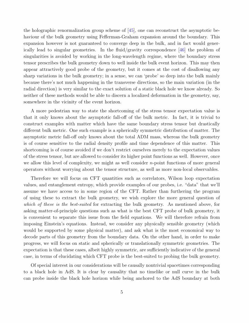
Fig. 2: Effective potentials for global Schwarzschild-AdS5, as L is varied at fixed E (left) and as E is

varied at fixed L (right), both for fixed r+ = 1. (left): L = 0, . . . , 3 in increments of 1/4 from

bottom right (red) to top right (purple) at E = 2. (right): E = 0, . . . , 4 in increments of 1/2

from top (red) to bottom (purple) at L = 2.

This suggests that to minimize r∗ along either family of curves, we need to lower L2 or raise

E2 respectively until Veff has local maximum at zero, so that Veff(r∗) = V ′eff(r∗) = 0. This will

correspond to unstable circular orbit, and by the above constructive argument exists for a range

of energies, each of which determines the requisite angular momentum. In other words, there

will be a one-dimensional curve in (E,L) space along which the corresponding geodesic has a

circular orbit. It then remains to find where along this curve is r∗ minimized.

From (2.26) and the considerations of the preceding discussion, we see that we can lower r∗arbitrarily close to r+ by taking E = 0 (so that Veff(r+) = 0) and adjusting L to the correct

value (so that V ′eff(r+) = 0). For general r, the latter would be achieved by L2 = r3 h′(r)2h(r)+r h′(r)

,

but at the horizon, this becomes simply L2 = r2+. Recall that for E = 0, Veff = 1

h(r)

(L2

r2 − 1)

,

which has zeros at r = r+ and r = L. A spacelike geodesic with E = 0 and L2 = r2+ would

get trapped in a circular orbit at the horizon, so in order to consider a probe geodesic, we need

to take L2 slightly larger. Nevertheless, this means that we can use probe geodesics to reach

arbitrarily close to the horizon.

However, the nearer r2∗ = L2 is to r2

+, the longer the geodesic spends in the vicinity of

the horizon, so the larger ∆ϕ is. Moreover, its regularized proper length likewise increases

as L → r+, so such geodesics will be highly subdominant to the one anchored at the same

boundary points with ∆ϕ mod 2π. Restricting ∆ϕ < 2π then sets a lower bound on r∗ which

lies some finite distance above the horizon.13

13 Note that already for ∆ϕ > π, there exists a shorter geodesic (on the other side of the black hole) which

connects the same boundary points. This means that the corresponding CFT probe will not have the dominant

behaviour determined by this geodesic.

18

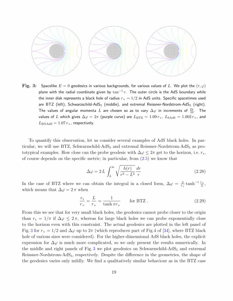
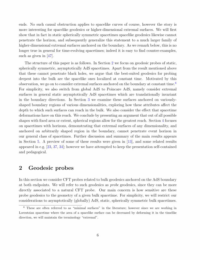
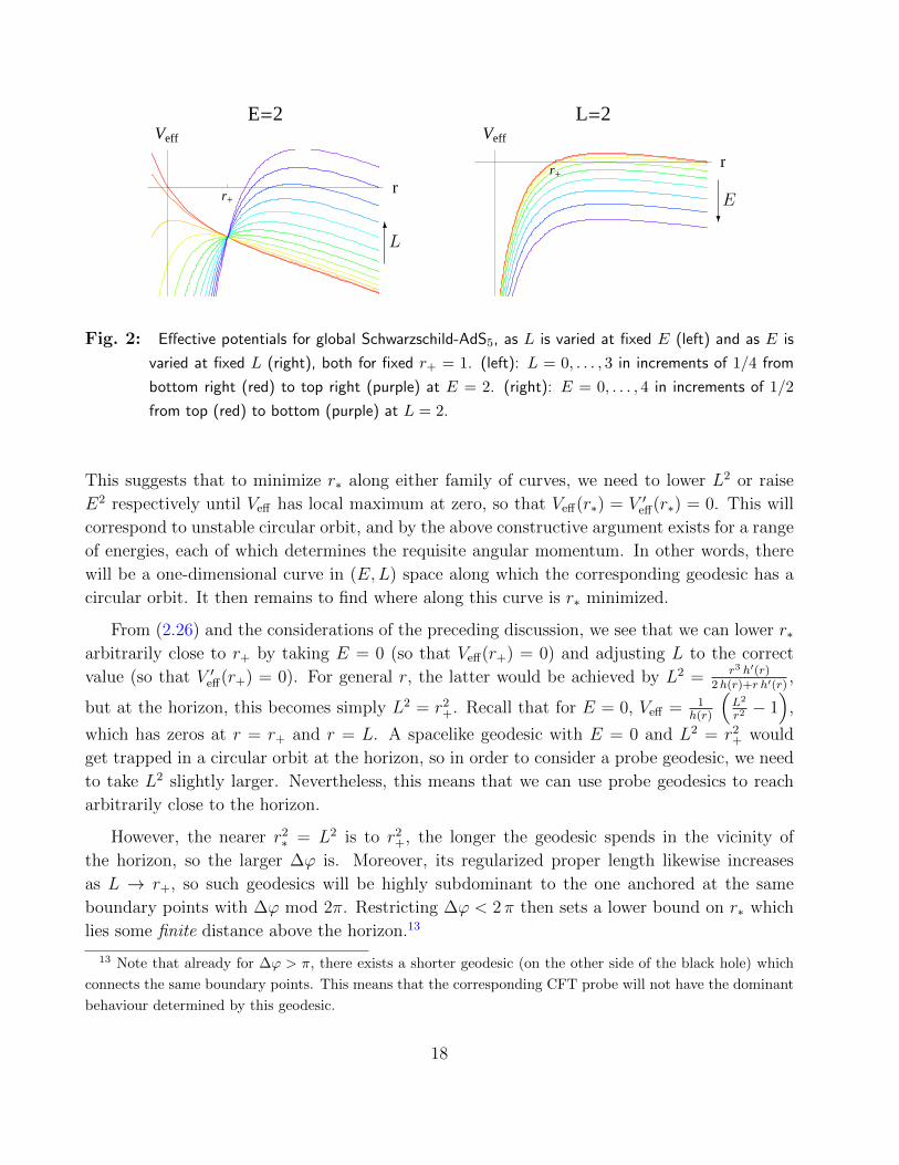
Fig. 3: Spacelike E = 0 geodesics in various backgrounds, for various values of L. We plot the (r, ϕ)

plane with the radial coordinate given by tan−1 r. The outer circle is the AdS boundary while

the inner disk represents a black hole of radius r+ = 1/2 in AdS units. Specific spacetimes used

are BTZ (left), Schwarzschild-AdS5 (middle), and extremal Reissner-Nordstrom-AdS5 (right).

The values of angular momenta L are chosen so as to vary ∆ϕ in increments of 2π10 . The

values of L which gives ∆ϕ = 2π (purple curve) are LBTZ = 1.09 r+, LSAdS = 1.002 r+, and

LRNAdS = 1.07 r+, respectively.

To quantify this observation, let us consider several examples of AdS black holes. In par-

ticular, we will use BTZ, Schwarzschild-AdS5 and extremal Reissner-Nordstrom-AdS5 as pro-

totypical examples. How close can the probe geodesic with ∆ϕ ≤ 2π get to the horizon, i.e. r∗,

of course depends on the specific metric; in particular, from (2.5) we know that

∆ϕ = 2L

∫ ∞L

√h(r)

r2 − L2

dr

r(2.28)

In the case of BTZ where we can obtain the integral in a closed form, ∆ϕ = 2r+

tanh−1 r+L

,

which means that ∆ϕ = 2π when

r∗r+

=L

r+

=1

tanhπr+

for BTZ . (2.29)

From this we see that for very small black holes, the geodesics cannot probe closer to the origin

than r∗ = 1/π if ∆ϕ ≤ 2π, whereas for large black holes we can probe exponentially close

to the horizon even with this constraint. The actual geodesics are plotted in the left panel of

Fig. 3 for r+ = 1/2 and ∆ϕ up to 2π (which reproduces part of Fig.4 of [34], where BTZ black

hole of various sizes were considered). For the higher-dimensional AdS black holes, the explicit

expression for ∆ϕ is much more complicated, so we only present the results numerically. In

the middle and right panels of Fig. 3 we plot geodesics on Schwarzschild-AdS5 and extremal

Reissner-Nordstrom-AdS5, respectively. Despite the difference in the geometries, the shape of

the geodesics varies only mildly. We find a qualitatively similar behaviour as in the BTZ case

19

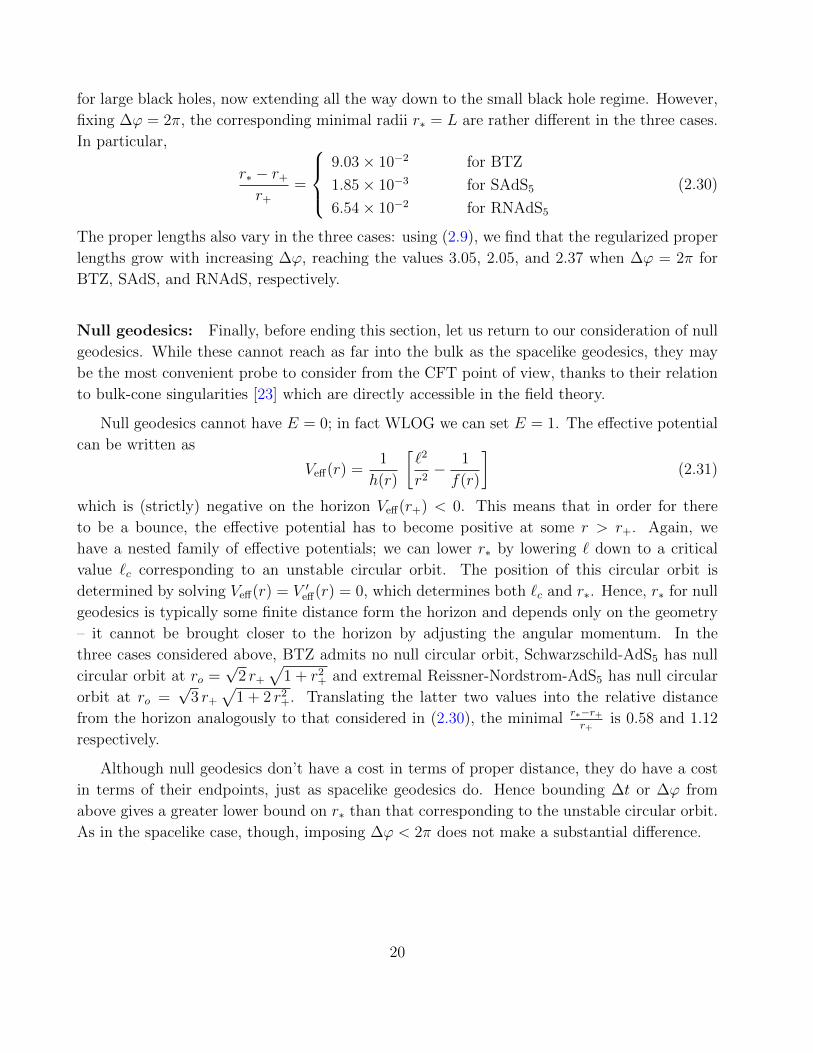
for large black holes, now extending all the way down to the small black hole regime. However,

fixing ∆ϕ = 2π, the corresponding minimal radii r∗ = L are rather different in the three cases.

In particular,

r∗ − r+

r+

=

9.03× 10−2 for BTZ

1.85× 10−3 for SAdS5

6.54× 10−2 for RNAdS5

(2.30)

The proper lengths also vary in the three cases: using (2.9), we find that the regularized proper

lengths grow with increasing ∆ϕ, reaching the values 3.05, 2.05, and 2.37 when ∆ϕ = 2π for

BTZ, SAdS, and RNAdS, respectively.

Null geodesics: Finally, before ending this section, let us return to our consideration of null

geodesics. While these cannot reach as far into the bulk as the spacelike geodesics, they may

be the most convenient probe to consider from the CFT point of view, thanks to their relation

to bulk-cone singularities [23] which are directly accessible in the field theory.

Null geodesics cannot have E = 0; in fact WLOG we can set E = 1. The effective potential

can be written as

Veff(r) =1

h(r)

[`2

r2− 1

f(r)

](2.31)

which is (strictly) negative on the horizon Veff(r+) < 0. This means that in order for there

to be a bounce, the effective potential has to become positive at some r > r+. Again, we

have a nested family of effective potentials; we can lower r∗ by lowering ` down to a critical

value `c corresponding to an unstable circular orbit. The position of this circular orbit is

determined by solving Veff(r) = V ′eff(r) = 0, which determines both `c and r∗. Hence, r∗ for null

geodesics is typically some finite distance form the horizon and depends only on the geometry

– it cannot be brought closer to the horizon by adjusting the angular momentum. In the

three cases considered above, BTZ admits no null circular orbit, Schwarzschild-AdS5 has null

circular orbit at ro =√

2 r+

√1 + r2

+ and extremal Reissner-Nordstrom-AdS5 has null circular

orbit at ro =√

3 r+

√1 + 2 r2

+. Translating the latter two values into the relative distance

from the horizon analogously to that considered in (2.30), the minimal r∗−r+r+

is 0.58 and 1.12

respectively.

Although null geodesics don’t have a cost in terms of proper distance, they do have a cost

in terms of their endpoints, just as spacelike geodesics do. Hence bounding ∆t or ∆ϕ from

above gives a greater lower bound on r∗ than that corresponding to the unstable circular orbit.

As in the spacelike case, though, imposing ∆ϕ < 2π does not make a substantial difference.

20

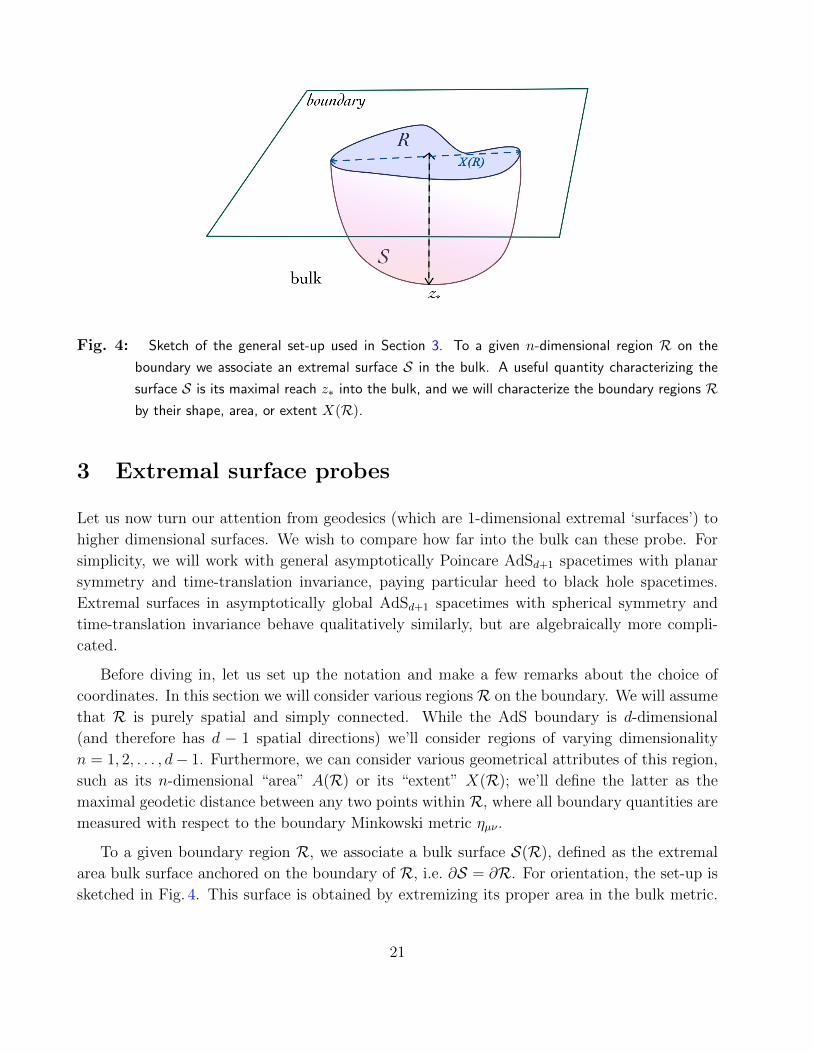
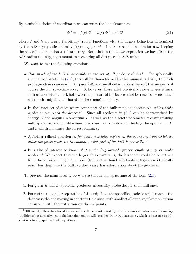
Fig. 4: Sketch of the general set-up used in Section 3. To a given n-dimensional region R on the

boundary we associate an extremal surface S in the bulk. A useful quantity characterizing the

surface S is its maximal reach z∗ into the bulk, and we will characterize the boundary regions Rby their shape, area, or extent X(R).

3 Extremal surface probes

Let us now turn our attention from geodesics (which are 1-dimensional extremal ‘surfaces’) to

higher dimensional surfaces. We wish to compare how far into the bulk can these probe. For

simplicity, we will work with general asymptotically Poincare AdSd+1 spacetimes with planar

symmetry and time-translation invariance, paying particular heed to black hole spacetimes.

Extremal surfaces in asymptotically global AdSd+1 spacetimes with spherical symmetry and

time-translation invariance behave qualitatively similarly, but are algebraically more compli-

cated.

Before diving in, let us set up the notation and make a few remarks about the choice of

coordinates. In this section we will consider various regions R on the boundary. We will assume

that R is purely spatial and simply connected. While the AdS boundary is d-dimensional

(and therefore has d − 1 spatial directions) we’ll consider regions of varying dimensionality

n = 1, 2, . . . , d− 1. Furthermore, we can consider various geometrical attributes of this region,

such as its n-dimensional “area” A(R) or its “extent” X(R); we’ll define the latter as the

maximal geodetic distance between any two points within R, where all boundary quantities are

measured with respect to the boundary Minkowski metric ηµν .

To a given boundary region R, we associate a bulk surface S(R), defined as the extremal

area bulk surface anchored on the boundary of R, i.e. ∂S = ∂R. For orientation, the set-up is

sketched in Fig. 4. This surface is obtained by extremizing its proper area in the bulk metric.

21

Although by virtue of extending to the AdS boundary the area of S is infinite, the problem of

finding the extremal surface is nevertheless well-defined. In practice when comparing this bulk

probe with the corresponding CFT quantity, we regulate to get a finite answer (as described

e.g. in [37]; see also [48, 49] for more recent discussion). Since we will restrict our considerations

to bulk spacetimes with planar symmetry and time-translation invariance, we can define the

bulk radial direction unambiguously (i.e., geometrically), and thereby compare the “reach” of

various surfaces S in a natural way.

Having clear definition of the bulk radial direction everywhere in the bulk spacetime (as the

unique direction orthogonal to all the other symmetries), all that remains is to find a convenient

gauge in which to compare the reach of various surfaces in different spacetimes consistently.

For this task, it is simplest to pick Fefferman-Graham coordinates, in which the bulk metric

takes the form

ds2 =1

z2

[−g(z) dt2 + k(z) dxi dx

i + dz2]

(3.1)

with i = 1, . . . , d − 1. This form is uniquely defined for any given spacetime by requiring

gzz = 1/z2 and gzµ = 0. Phrased more geometrically, z is related to the affine parameter λ

(measuring the proper length) along an ingoing radial spacelike geodesic as z = eλ. Note that

z = 0 corresponds to the AdS boundary. We can now define the “maximal reach” of S, z∗ by

the largest z value along S.

In practice, however, (3.1) is not necessarily the best gauge for writing the equations of

motion for the surfaces we will study, because the Lagrangian for n-dimensional extremal

surface would contain factors of k(z)n−1

2 . It will turn out to be simpler for our considerations

to use a different radial coordinate, z, such that we keep gii = 1/z2, and instead shift the

non-trivial z-dependence to gzz, as is more conventional in context of studying black holes:

ds2 =1

z2

[−f(z) dt2 + dxi dx

i + h(z) dz2]

(3.2)

Note the use of tilde above z to emphasize the distinction from the Fefferman-Graham coordi-

nates; we’ll use this convention throughout the present section. In both (3.1) and (3.2) the AdS

asymptotics requires the functions g, k → 1 as z → 0 and14 f, h → 1 as z → 0. For example,

the planar Schwarzschild-AdS5 spacetime corresponds to

f(z) = 1− z4

z4+

, h(z) =1

1− z4

z4+

, g(z) =

(1− z4

z4+

)2

1 + z4

z4+

, and k(z) = 1 +z4

z4+

. (3.3)

In the coordinates of (3.2), we will define the maximal reach of S by the largest value of z

attained by S, and denote it by z∗.

14The functions f and h are of course distinct from those used in the global AdS calculations of the previous

section.

22

Whereas it will be easier to find the reach of S in terms of z∗, we will convert it to z∗ for

purposes of comparison between spacetimes. In particular, to convert between (3.1) and (3.2),

we use the coordinate transformation (obtained by matching gii)

z =z√k(z)

(3.4)

which then allows us to relate the metric functions:

h(z) =1

k(z)

[d

dz

(z√k(z)

)]−2

=

(1− z

2

k′(z)

k(z)

)−2

and f(z) =g(z)

k(z). (3.5)

Once we know k(z), we need to invert (3.4) to find z(z), and hence z∗ from z∗. This however

assumes that z(z) is a strictly monotonically increasing function, which a-priori need not be

the case. Nevertheless, we will now argue that within the entire region of relevance, i.e. where

S can possibly reach, z(z) does remain monotonic. The argument relies on a statement whose

full proof we leave to Section 4, that extremal surfaces can’t reach past horizons whilst fully

anchored on the boundary. The fact that outside the horizon, where S can reach, z(z) must be

monotonic, can be seen as follows.

Observe that z(z) is monotonic as long as dzdz> 0. Now suppose this condition is violated

at some z0. In other words, ddz

(z/√k(z)) |z0= 0. Then we see from (3.5) that this means h(z)

diverges at the corresponding value of z(z0). Assuming the full metric is non-singular there,

this means that z = z0 describes a null surface, specifically a horizon. For static spacetimes,

this is both a Killing horizon for ∂at as well as an event horizon for the bulk spacetime. Our

assertion (proved Section 4) that extremal surfaces can’t reach past horizons then implies that

our extremal surface S cannot reach that far, i.e., z∗ < z0. Hence within the entire region of

relevance for any surface S, (3.4) is necessarily monotonic and therefore invertible.

We now consider specific cases of extremal surfaces S anchored on various regions R in

various bulk geometries, building up from the simplest case in a self-contained manner. Apart

from taking as R as an infinite strip or a round ball in pure AdS (which have already been

partly considered previously, cf. e.g. [37, 34]), we generalize these constructions to arbitrary

asymptotically Poincare AdS spacetimes of the form (3.2), giving explicit results for planar

Schwarzschild-AdS5 and extremal Reissner-Nordstrom-AdS5. We end the section by discussing

extremal n-surfaces in AdSd+1 ending on generic regions, to see how different shapes of R affect

the reach z∗ of S. In the next section, we proceed to generalize the set-up even further, and

consider arbitrary regions R in general asymptotically Poincare AdS spacetimes of the form

(3.2), in order to ascertain in full generality that S cannot probe past a bulk horizon.

23

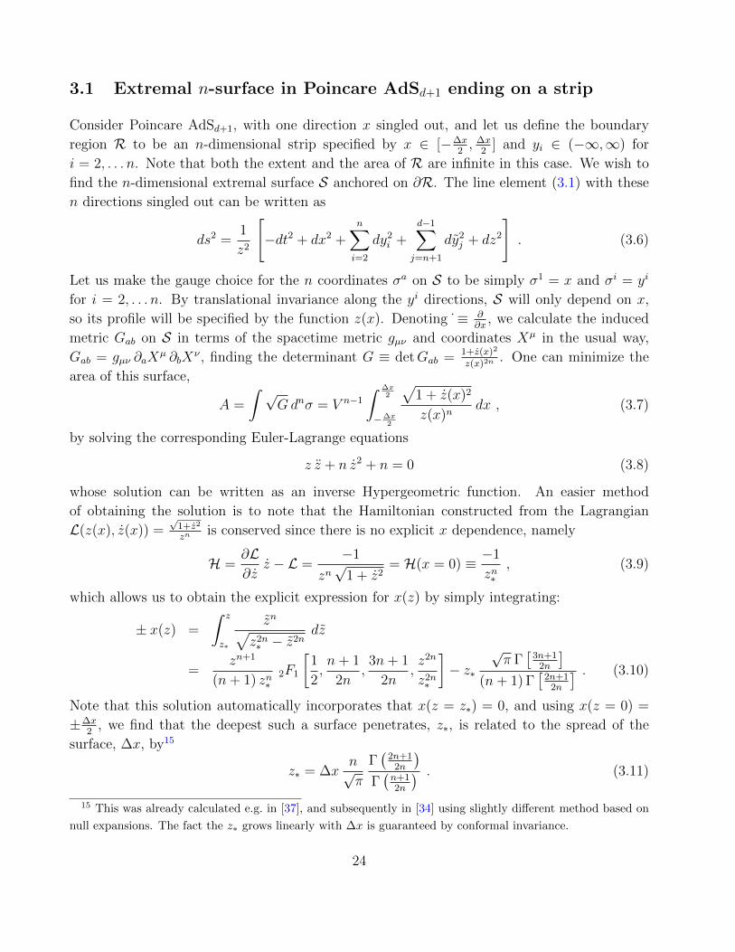
3.1 Extremal n-surface in Poincare AdSd+1 ending on a strip

Consider Poincare AdSd+1, with one direction x singled out, and let us define the boundary

region R to be an n-dimensional strip specified by x ∈ [−∆x2, ∆x

2] and yi ∈ (−∞,∞) for

i = 2, . . . n. Note that both the extent and the area of R are infinite in this case. We wish to

find the n-dimensional extremal surface S anchored on ∂R. The line element (3.1) with these

n directions singled out can be written as

ds2 =1

z2

[−dt2 + dx2 +

n∑i=2

dy2i +

d−1∑j=n+1

dy2j + dz2

]. (3.6)

Let us make the gauge choice for the n coordinates σa on S to be simply σ1 = x and σi = yi

for i = 2, . . . n. By translational invariance along the yi directions, S will only depend on x,

so its profile will be specified by the function z(x). Denoting ˙≡ ∂∂x

, we calculate the induced

metric Gab on S in terms of the spacetime metric gµν and coordinates Xµ in the usual way,

Gab = gµν ∂aXµ ∂bX

ν , finding the determinant G ≡ detGab = 1+z(x)2

z(x)2n . One can minimize the

area of this surface,

A =

∫ √Gdnσ = V n−1

∫ ∆x2

−∆x2

√1 + z(x)2

z(x)ndx , (3.7)

by solving the corresponding Euler-Lagrange equations

z z + n z2 + n = 0 (3.8)

whose solution can be written as an inverse Hypergeometric function. An easier method

of obtaining the solution is to note that the Hamiltonian constructed from the Lagrangian

L(z(x), z(x)) =√

1+z2

znis conserved since there is no explicit x dependence, namely

H =∂L∂z

z − L =−1

zn√

1 + z2= H(x = 0) ≡ −1

zn∗, (3.9)

which allows us to obtain the explicit expression for x(z) by simply integrating:

± x(z) =

∫ z

z∗

zn√z2n∗ − z2n

dz

=zn+1

(n+ 1) zn∗2F1

[1

2,n+ 1

2n,3n+ 1

2n,z2n

z2n∗

]− z∗

√π Γ[

3n+12n

](n+ 1) Γ

[2n+1

2n

] . (3.10)

Note that this solution automatically incorporates that x(z = z∗) = 0, and using x(z = 0) =

±∆x2

, we find that the deepest such a surface penetrates, z∗, is related to the spread of the

surface, ∆x, by15

z∗ = ∆xn√π

Γ(

2n+12n

)Γ(n+12n

) . (3.11)

15 This was already calculated e.g. in [37], and subsequently in [34] using slightly different method based on

null expansions. The fact the z∗ grows linearly with ∆x is guaranteed by conformal invariance.

24

-z* z*

x

z*

z

2 4 6 8n

0.5

1.0

1.5

2.0

2.5

z*Dx

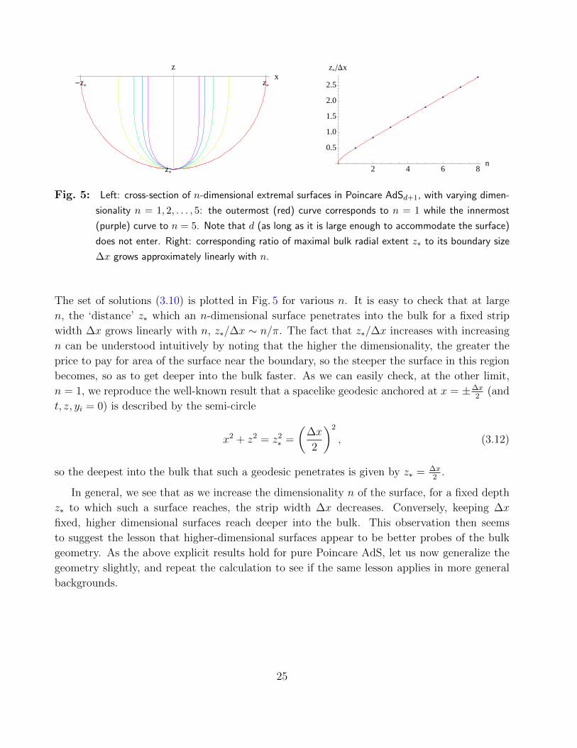
Fig. 5: Left: cross-section of n-dimensional extremal surfaces in Poincare AdSd+1, with varying dimen-

sionality n = 1, 2, . . . , 5: the outermost (red) curve corresponds to n = 1 while the innermost

(purple) curve to n = 5. Note that d (as long as it is large enough to accommodate the surface)

does not enter. Right: corresponding ratio of maximal bulk radial extent z∗ to its boundary size

∆x grows approximately linearly with n.

The set of solutions (3.10) is plotted in Fig. 5 for various n. It is easy to check that at large

n, the ‘distance’ z∗ which an n-dimensional surface penetrates into the bulk for a fixed strip

width ∆x grows linearly with n, z∗/∆x ∼ n/π. The fact that z∗/∆x increases with increasing

n can be understood intuitively by noting that the higher the dimensionality, the greater the

price to pay for area of the surface near the boundary, so the steeper the surface in this region

becomes, so as to get deeper into the bulk faster. As we can easily check, at the other limit,

n = 1, we reproduce the well-known result that a spacelike geodesic anchored at x = ±∆x2

(and

t, z, yi = 0) is described by the semi-circle

x2 + z2 = z2∗ =

(∆x

2

)2

, (3.12)

so the deepest into the bulk that such a geodesic penetrates is given by z∗ = ∆x2

.

In general, we see that as we increase the dimensionality n of the surface, for a fixed depth

z∗ to which such a surface reaches, the strip width ∆x decreases. Conversely, keeping ∆x

fixed, higher dimensional surfaces reach deeper into the bulk. This observation then seems

to suggest the lesson that higher-dimensional surfaces appear to be better probes of the bulk

geometry. As the above explicit results hold for pure Poincare AdS, let us now generalize the

geometry slightly, and repeat the calculation to see if the same lesson applies in more general

backgrounds.

25

3.2 Extremal n-surface in asymptotically AdSd+1 ending on a strip

We want to compare the reach z∗ of an extremal surface S corresponding to the infinite strip

R considered in Section 3.1, in the more general bulk spacetimes (3.1), or more conveniently

(3.2). It turns out easier to obtain z∗ first and then use the conversion between the respective

bulk radial coordinates given by (3.4) to obtain z∗. It will also be convenient to split the xi

directions in the same manner as in Section 3.1 above. To that end, we write the bulk metric

in the form

ds2 =1

z2

[−f(z) dt2 + dx2 +

n∑i=2

dy2i +

d−1∑j=n+1

dy2j + h(z) dz2

](3.13)

where we use the tilde on z to emphasize the distinction from the Fefferman-Graham coordi-

nates.

Note that since the spacetime (3.13) is static, the extremal surface will lie on constant t

spacelike slice of the bulk, so the metric function f(z) will not enter our calculations. Analo-

gously to (3.7), the area of this extremal surface is

A = V n−1

∫ ∆x2

−∆x2

√1 + h(z) ˙z(x)2

z(x)ndx (3.14)

and we can again use the conservation of Hamiltonian to write the profile x(z) in integral form:

± x(z) =

∫ z

z∗

√h(z) zn√z2n∗ − z2n

dz . (3.15)

To proceed further, we have to specify h(z). However, if the spacetime is smooth and asymp-

totically AdS, we can Taylor-expand√h(z) around z = 0 and integrate each term in the

expansion. Defining √h(z) =

∞∑m=0

qm zm (3.16)

(with q0 = 1), we have, analogously to (3.10),

± x(z) =∞∑m=0

qm

∫ z

z∗

zn+m√z2n∗ − z2n

dz

=zn+1

zn∗

∞∑m=0

qm zm

n+m+ 12F1

[1

2,n+m+ 1

2n,3n+m+ 1

2n,z2n

z2n∗

]−√π z∗

∞∑m=0

qm zm 1

m+ 1

Γ[n+m+1

2n

]Γ[m+12n

] . (3.17)

26

We can now read off the width of the strip ∆xn for the n-dimensional extremal surface in

terms of z∗ and qm:

∆xn =

√π

n

∞∑m=1

qm−1 zm∗

Γ[n+m

2n

]Γ[

2n+m2n

] . (3.18)

It is easy to see that in the large-n limit,

∆xn ∼ z∗√h(z∗)

π

nas n→∞ , (3.19)

which indeed demonstrates monotonicity with n in the large n regime for any spacetime of the

form (3.13). However, in our set-up n ≤ d − 1, so it’s more convenient to examine (3.18) for

small n explicitly by evaluating the Gamma functions. The ratio of the Gamma functions in

(3.18) scales as ∼√

1/m at large m, however these coefficients are slightly larger than 1 for

small m, so we cannot straightforwardly use (3.19) as an upper bound for any n. To build

intuition, let us then simplify the problem further.

To this end, let us consider just the first subleading term in the expansion (3.16). In

particular, let√h(z) = 1 + qd z

d. Then ∆xn in (3.18) consists of only two terms, and we can

check at which value of qd zd∗ does ∆xn become smaller than ∆xm for some m < n. It turns

out that this value is always negative, and moreover it also necessarily renders ∆xn negative.16

This suggests that in the physical regime, ∆xn is indeed monotonically decreasing with n over

the full range of n, and of course increasing with z∗; so conversely, if we fix ∆x, then z∗ increases

with increasing n in this larger class of bulk geometries, just as it did for pure AdS.

Having motivated our expectations, we now argue this in far greater generality by consid-

ering the integral form of ∆x given by (3.15), which we can rewrite more suggestively as

∆x = 2

∫ z∗

0

√h(z)√

(z∗/z)2n − 1dz . (3.20)

For fixed z∗ (and fixed h(z) > 0), the denominator in the integrand is larger for larger n when

z ∈ (0, z∗), which implies that the full integral is smaller for larger n. This proves that ∆x/z∗decreases with n, so that at fixed ∆x, z∗ increases with n – i.e., higher-dimensional surfaces

probe deeper.

Pure AdS yields largest z∗/∆xn: Now that we have analyzed the effect of varying n in a

fixed spacetime, let us fix n and instead consider the effect of varying the spacetime, i.e., explore

the effect that the deformation h(z) in (3.13) has on the extremal surfaces. From (3.20), we

immediately see that if h(z) ≥ 1 ∀ z ∈ (0, z∗), then the corresponding ∆x is greater than the

16 The former is easy to see; the latter, although somewhat tedious, can likewise be verified algebraically

using monotonicity properties of the Gamma functions involved.

27

pure AdS (h(z) = 1) value, for any n. As we see from (3.3), the planar Schwarzschild-AdS black

hole certainly satisfies h(z) ≥ 1, and we expect more generally that this condition would hold

for physically sensible situations – in other words, we expect that any physically admissible

matter would create a gravitational potential well. This is easy to see asymptotically. Let us

again start by considering just the leading order correction to pure AdS,√h(z) = 1 + qd z

d.

(Note that from (3.18) we immediately recover that for any n, if qd > 0, ∆xn at fixed z∗is greater than the corresponding value in pure AdS.) So all that remains is to establish the

physically relevant sign of qd.

The physically relevant sign of qd is the one which yields a physically sensible stress tensor on

the boundary, namely one with non-negative energy density, pressure, etc.. So in order to deter-

mine which class of bulk deformations is physically sensible, we will first extract the boundary

stress tensor. One can do this by several methods; e.g. we can use the Balasubramanian-Kraus

construction [50] in the present coordinates, or we can use the de Haro et.al.’s prescription [45]

to read off the stress tensor from the metric as expressed in Fefferman-Graham coordinates.

Let us illustrate this in 4+1 bulk dimensions. Writing the metric in Fefferman-Graham

coordinates as

ds2 =1

z2

[dz2 +

(g(0)µν + z2 g(2)

µν + z4 g(4)µν + . . .

)dxµ dxν

](3.21)

with g(0)µν = ηµν implies that g

(2)µν = 0, and g

(4)µν ∝ 〈Tµν〉, where 〈Tµν〉 is the expectation value of

the boundary stress tensor. Letting Tµν take the perfect fluid form,

Tµν = ρ uµ uν + P (ηµν + uµ uν) (3.22)

gives

ds2 =1

z2

[−(1− ρ z4

)dt2 +

(1 + P z4

)dxi dx

i + dz2]. (3.23)

For example, for the planar Schwarzschild-AdS black hole, expanding the metric (3.3) to O(z4)

gives the known values

ρ =3

z4+

= 3π4 T 4 , P =1

z4+

= π4 T 4 =ρ

3. (3.24)

We invert (3.4) to relate the Fefferman-Graham form (3.23) to the form (3.2) used above,

specifically

z2 =z2

1 + P z4⇐⇒ z2 =

1−√

1− 4P z4

2P z2. (3.25)

Keeping only terms up to O(z4), we can expand (3.2) as

ds2 =1

z2

[−(1− [ρ+ P ] z4) dt2 + dxi dx

i + (1 + 4P z4) dz2]

(3.26)

which allows us to identify √f(z) = 1 + q4 z

4 = 1 + 2P z4 . (3.27)

28

In particular, this means that the physically sensible sign of q4 = 2P is indeed positive.

We have now established that asymptotically, a physically sensible deformation of AdS

requires the leading correction to h(z) to be positive. Moreover, as exemplified by the black

hole metric (3.3) and argued more generally in Section 4, h(z) has to get large near the horizon

of any black hole. Hence what remains unknown is the region between the horizon and the

asymptopia.

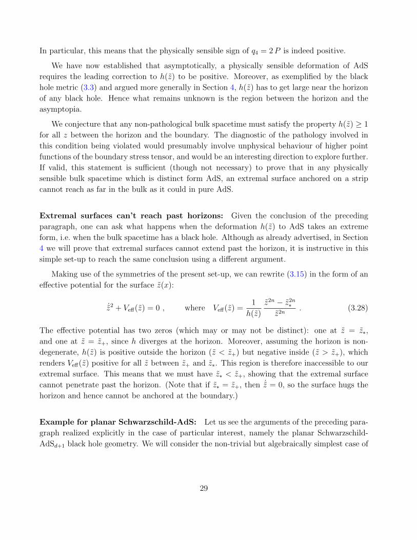
We conjecture that any non-pathological bulk spacetime must satisfy the property h(z) ≥ 1

for all z between the horizon and the boundary. The diagnostic of the pathology involved in

this condition being violated would presumably involve unphysical behaviour of higher point

functions of the boundary stress tensor, and would be an interesting direction to explore further.

If valid, this statement is sufficient (though not necessary) to prove that in any physically

sensible bulk spacetime which is distinct form AdS, an extremal surface anchored on a strip

cannot reach as far in the bulk as it could in pure AdS.

Extremal surfaces can’t reach past horizons: Given the conclusion of the preceding

paragraph, one can ask what happens when the deformation h(z) to AdS takes an extreme

form, i.e. when the bulk spacetime has a black hole. Although as already advertised, in Section

4 we will prove that extremal surfaces cannot extend past the horizon, it is instructive in this

simple set-up to reach the same conclusion using a different argument.

Making use of the symmetries of the present set-up, we can rewrite (3.15) in the form of an

effective potential for the surface z(x):

˙z2 + Veff(z) = 0 , where Veff(z) =1

h(z)

z2n − z2n∗

z2n. (3.28)

The effective potential has two zeros (which may or may not be distinct): one at z = z∗,

and one at z = z+, since h diverges at the horizon. Moreover, assuming the horizon is non-

degenerate, h(z) is positive outside the horizon (z < z+) but negative inside (z > z+), which

renders Veff(z) positive for all z between z+ and z∗. This region is therefore inaccessible to our

extremal surface. This means that we must have z∗ < z+, showing that the extremal surface

cannot penetrate past the horizon. (Note that if z∗ = z+, then ˙z = 0, so the surface hugs the

horizon and hence cannot be anchored at the boundary.)

Example for planar Schwarzschild-AdS: Let us see the arguments of the preceding para-

graph realized explicitly in the case of particular interest, namely the planar Schwarzschild-

AdSd+1 black hole geometry. We will consider the non-trivial but algebraically simplest case of

29

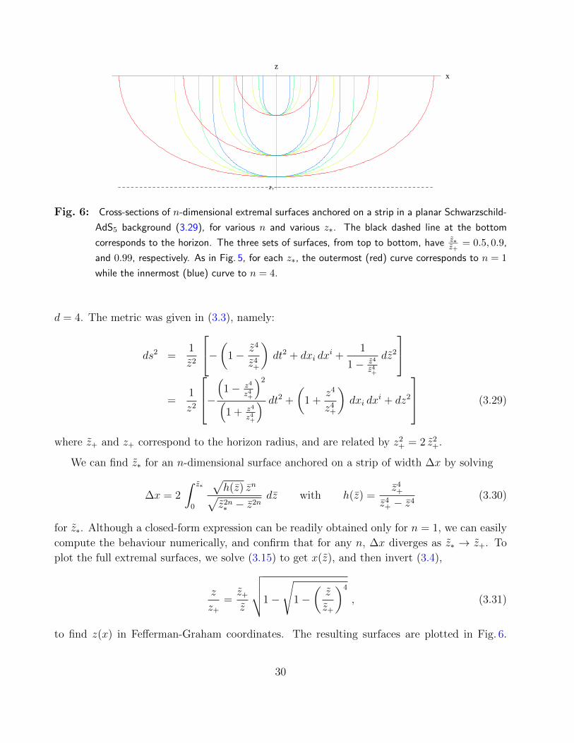
x

z+

z

Fig. 6: Cross-sections of n-dimensional extremal surfaces anchored on a strip in a planar Schwarzschild-

AdS5 background (3.29), for various n and various z∗. The black dashed line at the bottom

corresponds to the horizon. The three sets of surfaces, from top to bottom, have z∗z+

= 0.5, 0.9,

and 0.99, respectively. As in Fig. 5, for each z∗, the outermost (red) curve corresponds to n = 1

while the innermost (blue) curve to n = 4.

d = 4. The metric was given in (3.3), namely:

ds2 =1

z2

−(1− z4

z4+

)dt2 + dxi dx

i +1

1− z4

z4+

dz2

=

1

z2

−(

1− z4

z4+

)2(1 + z4

z4+

) dt2 +

(1 +

z4

z4+

)dxi dx

i + dz2

(3.29)

where z+ and z+ correspond to the horizon radius, and are related by z2+ = 2 z2

+.

We can find z∗ for an n-dimensional surface anchored on a strip of width ∆x by solving

∆x = 2

∫ z∗

0

√h(z) zn√z2n∗ − z2n

dz with h(z) =z4

+

z4+ − z4

(3.30)

for z∗. Although a closed-form expression can be readily obtained only for n = 1, we can easily

compute the behaviour numerically, and confirm that for any n, ∆x diverges as z∗ → z+. To

plot the full extremal surfaces, we solve (3.15) to get x(z), and then invert (3.4),

z

z+

=z+

z

√√√√1−

√1−

(z

z+

)4

, (3.31)

to find z(x) in Fefferman-Graham coordinates. The resulting surfaces are plotted in Fig. 6.

30

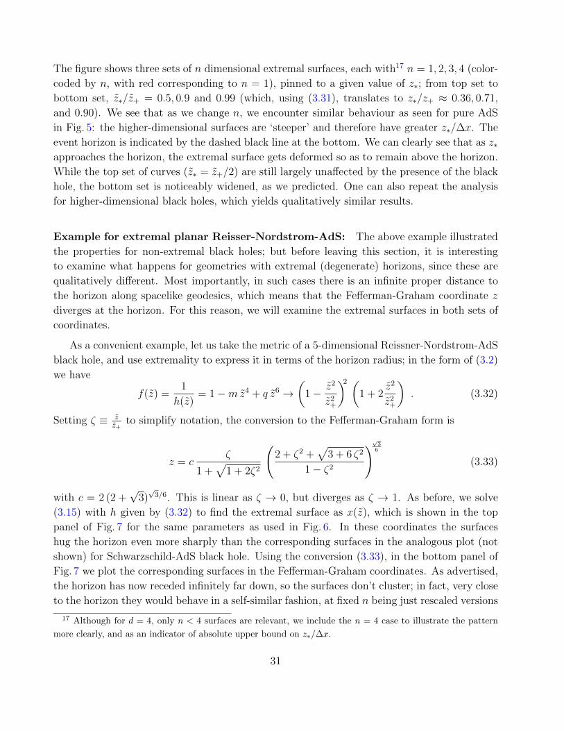
The figure shows three sets of n dimensional extremal surfaces, each with17 n = 1, 2, 3, 4 (color-

coded by n, with red corresponding to n = 1), pinned to a given value of z∗; from top set to

bottom set, z∗/z+ = 0.5, 0.9 and 0.99 (which, using (3.31), translates to z∗/z+ ≈ 0.36, 0.71,

and 0.90). We see that as we change n, we encounter similar behaviour as seen for pure AdS

in Fig. 5: the higher-dimensional surfaces are ‘steeper’ and therefore have greater z∗/∆x. The

event horizon is indicated by the dashed black line at the bottom. We can clearly see that as z∗approaches the horizon, the extremal surface gets deformed so as to remain above the horizon.

While the top set of curves (z∗ = z+/2) are still largely unaffected by the presence of the black

hole, the bottom set is noticeably widened, as we predicted. One can also repeat the analysis

for higher-dimensional black holes, which yields qualitatively similar results.

Example for extremal planar Reisser-Nordstrom-AdS: The above example illustrated

the properties for non-extremal black holes; but before leaving this section, it is interesting

to examine what happens for geometries with extremal (degenerate) horizons, since these are

qualitatively different. Most importantly, in such cases there is an infinite proper distance to

the horizon along spacelike geodesics, which means that the Fefferman-Graham coordinate z

diverges at the horizon. For this reason, we will examine the extremal surfaces in both sets of

coordinates.

As a convenient example, let us take the metric of a 5-dimensional Reissner-Nordstrom-AdS

black hole, and use extremality to express it in terms of the horizon radius; in the form of (3.2)

we have

f(z) =1

h(z)= 1−m z4 + q z6 →

(1− z2

z2+

)2 (1 + 2

z2

z2+

). (3.32)

Setting ζ ≡ zz+

to simplify notation, the conversion to the Fefferman-Graham form is

z = cζ

1 +√

1 + 2ζ2

(2 + ζ2 +

√3 + 6 ζ2

1− ζ2

)√36

(3.33)

with c = 2 (2 +√

3)√

3/6. This is linear as ζ → 0, but diverges as ζ → 1. As before, we solve

(3.15) with h given by (3.32) to find the extremal surface as x(z), which is shown in the top

panel of Fig. 7 for the same parameters as used in Fig. 6. In these coordinates the surfaces

hug the horizon even more sharply than the corresponding surfaces in the analogous plot (not

shown) for Schwarzschild-AdS black hole. Using the conversion (3.33), in the bottom panel of

Fig. 7 we plot the corresponding surfaces in the Fefferman-Graham coordinates. As advertised,

the horizon has now receded infinitely far down, so the surfaces don’t cluster; in fact, very close

to the horizon they would behave in a self-similar fashion, at fixed n being just rescaled versions

17 Although for d = 4, only n < 4 surfaces are relevant, we include the n = 4 case to illustrate the pattern

more clearly, and as an indicator of absolute upper bound on z∗/∆x.

31

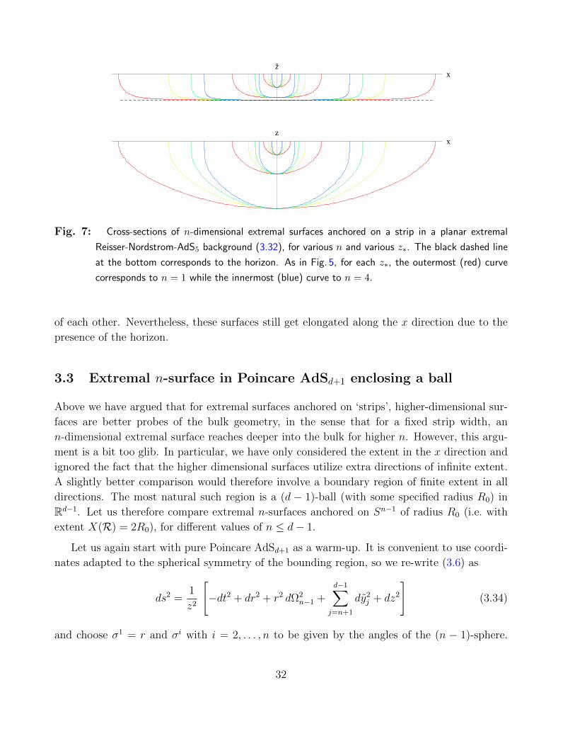
xz

xz

Fig. 7: Cross-sections of n-dimensional extremal surfaces anchored on a strip in a planar extremal

Reisser-Nordstrom-AdS5 background (3.32), for various n and various z∗. The black dashed line

at the bottom corresponds to the horizon. As in Fig. 5, for each z∗, the outermost (red) curve

corresponds to n = 1 while the innermost (blue) curve to n = 4.

of each other. Nevertheless, these surfaces still get elongated along the x direction due to the

presence of the horizon.

3.3 Extremal n-surface in Poincare AdSd+1 enclosing a ball

Above we have argued that for extremal surfaces anchored on ‘strips’, higher-dimensional sur-

faces are better probes of the bulk geometry, in the sense that for a fixed strip width, an

n-dimensional extremal surface reaches deeper into the bulk for higher n. However, this argu-

ment is a bit too glib. In particular, we have only considered the extent in the x direction and

ignored the fact that the higher dimensional surfaces utilize extra directions of infinite extent.

A slightly better comparison would therefore involve a boundary region of finite extent in all

directions. The most natural such region is a (d − 1)-ball (with some specified radius R0) in

Rd−1. Let us therefore compare extremal n-surfaces anchored on Sn−1 of radius R0 (i.e. with

extent X(R) = 2R0), for different values of n ≤ d− 1.

Let us again start with pure Poincare AdSd+1 as a warm-up. It is convenient to use coordi-

nates adapted to the spherical symmetry of the bounding region, so we re-write (3.6) as

ds2 =1

z2

[−dt2 + dr2 + r2 dΩ2

n−1 +d−1∑

j=n+1

dy2j + dz2

](3.34)

and choose σ1 = r and σi with i = 2, . . . , n to be given by the angles of the (n − 1)-sphere.

32

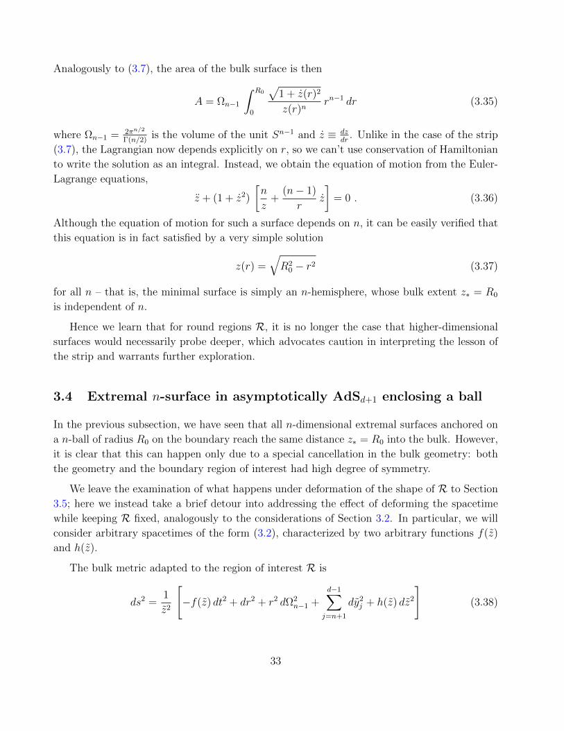
Analogously to (3.7), the area of the bulk surface is then

A = Ωn−1

∫ R0

0

√1 + z(r)2

z(r)nrn−1 dr (3.35)

where Ωn−1 = 2πn/2

Γ(n/2)is the volume of the unit Sn−1 and z ≡ dz

dr. Unlike in the case of the strip

(3.7), the Lagrangian now depends explicitly on r, so we can’t use conservation of Hamiltonian

to write the solution as an integral. Instead, we obtain the equation of motion from the Euler-

Lagrange equations,

z + (1 + z2)

[n

z+

(n− 1)

rz

]= 0 . (3.36)

Although the equation of motion for such a surface depends on n, it can be easily verified that

this equation is in fact satisfied by a very simple solution

z(r) =√R2

0 − r2 (3.37)

for all n – that is, the minimal surface is simply an n-hemisphere, whose bulk extent z∗ = R0

is independent of n.

Hence we learn that for round regions R, it is no longer the case that higher-dimensional

surfaces would necessarily probe deeper, which advocates caution in interpreting the lesson of

the strip and warrants further exploration.

3.4 Extremal n-surface in asymptotically AdSd+1 enclosing a ball

In the previous subsection, we have seen that all n-dimensional extremal surfaces anchored on

a n-ball of radius R0 on the boundary reach the same distance z∗ = R0 into the bulk. However,

it is clear that this can happen only due to a special cancellation in the bulk geometry: both

the geometry and the boundary region of interest had high degree of symmetry.

We leave the examination of what happens under deformation of the shape of R to Section

3.5; here we instead take a brief detour into addressing the effect of deforming the spacetime

while keeping R fixed, analogously to the considerations of Section 3.2. In particular, we will

consider arbitrary spacetimes of the form (3.2), characterized by two arbitrary functions f(z)

and h(z).

The bulk metric adapted to the region of interest R is

ds2 =1

z2

[−f(z) dt2 + dr2 + r2 dΩ2

n−1 +d−1∑

j=n+1

dy2j + h(z) dz2

](3.38)

33

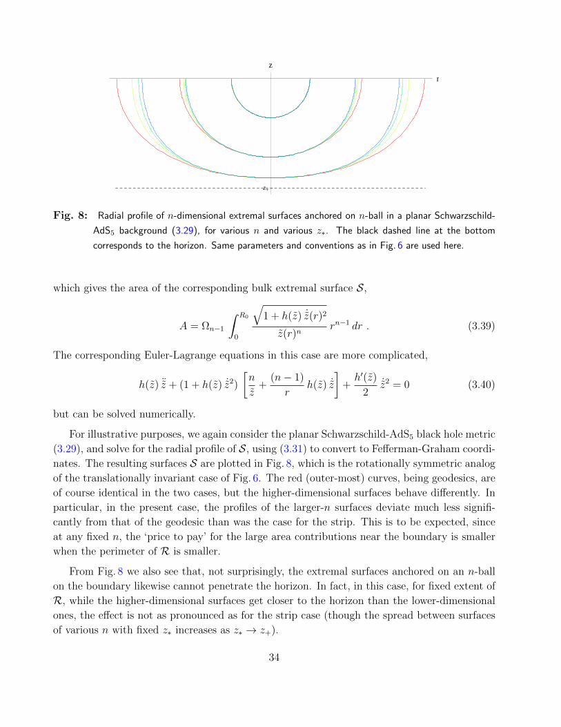
r

z+

z

Fig. 8: Radial profile of n-dimensional extremal surfaces anchored on n-ball in a planar Schwarzschild-

AdS5 background (3.29), for various n and various z∗. The black dashed line at the bottom

corresponds to the horizon. Same parameters and conventions as in Fig. 6 are used here.

which gives the area of the corresponding bulk extremal surface S,

A = Ωn−1

∫ R0

0

√1 + h(z) ˙z(r)2

z(r)nrn−1 dr . (3.39)

The corresponding Euler-Lagrange equations in this case are more complicated,

h(z) ¨z + (1 + h(z) ˙z2)

[n

z+

(n− 1)

rh(z) ˙z

]+h′(z)

2˙z2 = 0 (3.40)

but can be solved numerically.

For illustrative purposes, we again consider the planar Schwarzschild-AdS5 black hole metric

(3.29), and solve for the radial profile of S, using (3.31) to convert to Fefferman-Graham coordi-

nates. The resulting surfaces S are plotted in Fig. 8, which is the rotationally symmetric analog

of the translationally invariant case of Fig. 6. The red (outer-most) curves, being geodesics, are

of course identical in the two cases, but the higher-dimensional surfaces behave differently. In

particular, in the present case, the profiles of the larger-n surfaces deviate much less signifi-

cantly from that of the geodesic than was the case for the strip. This is to be expected, since

at any fixed n, the ‘price to pay’ for the large area contributions near the boundary is smaller

when the perimeter of R is smaller.

From Fig. 8 we also see that, not surprisingly, the extremal surfaces anchored on an n-ball

on the boundary likewise cannot penetrate the horizon. In fact, in this case, for fixed extent of

R, while the higher-dimensional surfaces get closer to the horizon than the lower-dimensional

ones, the effect is not as pronounced as for the strip case (though the spread between surfaces

of various n with fixed z∗ increases as z∗ → z+).

34

3.5 Extremal n-surface in Poincare AdSd+1 ending on generic regions

The motivation for the analysis of the preceding examples was to examine, for given amount of

boundary CFT data, which quantities are the best probes of the bulk geometry. However, it is

not entirely straightforward to compare boundary regions R of varying dimensionality. While

the depth z∗ to which their associated extremal surfaces S probe has a well-defined meaning

in general bulk spacetimes of the form (3.1), comparing how much boundary information they

require is trickier. For example, we can’t simply compare area of a 2-dimensional region with

a volume of a 3-dimensional region.

One way around this is to define a 1-dimensional quantity for any n-dimensional boundary

region R which characterizes its size. For example, as mentioned above, we can define the

extent X(R) of a region by the maximal distance18 between any two points within that region,

as indicated in Fig. 4. One can then ask, for a given extent of a region, what region ‘shape’

maximizes the depth z∗ to which the corresponding extremal surface reaches?

Alternately, at fixed n, we can compare the various attributes of n-dimensional regions of

different shapes. For example, we can ask: for a fixed n-volume on the boundary, what shape

of R is the most optimal for probing deepest into the bulk? As we will see momentarily, it

turns out that the answers to both of these questions in fact coincide. For convenience we will

then concentrate on the second question, and propose the following conjecture:

Conjecture: For a fixed area of a boundary region R, the shape of R which maximizes the

reach z∗ of the corresponding extremal surface S(R) is the round ball.

Before providing evidence for the conjecture, let us briefly discuss its implications. First of

all, it is a known geometrical fact that for a given volume of a region, its extent (as defined

above) is minimized when the region R is the round ball. Hence if the round ball is the region

whose bulk extremal surface S reaches deepest into the bulk amongst all regions with fixed

volume, then it is also the region whose S reaches deepest into the bulk amongst all regions

with fixed extent. In fact, using the results of the preceding subsection, the conjecture then

extends to any static asymptotically Poincare-AdS bulk geometry with planar symmetry. In

particular, the deepest into the bulk that any n-surface with volume VnRn0 could reach in any

asymptotically Poincare-AdS bulk of the form (3.1) is z∗ = R0 where z is the usual Fefferman-

Graham coordinate, and Vn = πn/2/Γ(n2

+ 1) is the volume of the unit n-ball. In the remainder

of this section, we will first give general arguments for our conjecture and then justify it with

explicit calculations for n = 2.

For the rest of this section, we consider pure Poincare AdS. The main intuition for the

18 Recall that when talking about lengths, volumes, etc., on the boundary, we use the Minkowski metric, i.e.

we drop the bulk warp factor 1z2 .

35

conjecture is built on the following simple observations:

• Round regions have manifestly greater z∗ than very elongated regions with the same

volume.

• In deforming a ball into e.g. an ellipsoid with elongation η, Poincare AdS does not have

enough structure to render z∗(η) a non-monotonic function. In other words, if a highly

elongated ellipsoid yields smaller z∗ than a round ball, then so should one with any

elongation.

• Finally, the dimensionality n of the surface is not crucial for these considerations.

The first statement is easy to see by comparing reach of S for an n-ball with that for a

finite strip: the n-ball of radius R0 will have z∗ = R0 (as we found in Section 3.3) and volume

V = VnRn0 . A ‘finite strip’ of dimensions (δ, L . . . , L will have volume V = δ Ln−1, so to match

the volumes we set δ = VnRn0/L

n−1. In the limit as L→∞, the ends of the strip become more

and more negligible for influencing the shape of the surface away from the ends, so the reach of

the surface is better and better approximated by that of an infinite strip of width δ, for which

(3.11) gives z∗ = γnRn0/L

n−1 R0 where γn ≡ nπn−1

2 Γ(

2n+12n

)/(Γ

(n+12n

)Γ(n+2

2

)) ∼ O(1).

The second expectation implies that we can likewise use surfaces anchored on regions given

by small deformations of the round ball. If by squeezing the ball slightly at fixed volume

the corresponding reach z∗ recedes, then we expect that the round ball allows the greatest z∗among all regions with fixed volume. This motivates the following explicit calculation: suppose

we deform a circular region R0 slightly, e.g. make it ellipsoidal. How does the corresponding

extremal surface respond? This question is amenable to perturbation theory: we linearize the

Euler-Lagrange equations defining the surface and solve them around the hemisphere to the

requisite order.

The last observation then suggests that it suffices to consider 2-dimensional surfaces; so in

what follows, we will take n = 2. We would like to fix the area of the 2-dimensional region

R on the boundary, and ask what shape allows for largest bulk reach z∗ of the corresponding

extremal surface. In practice, it will turn out simpler to fix z∗ and see how the area of Rresponds to changing the shape. However, we can easily convert to the fixed-area set-up using

scale invariance: since we are working in pure AdS, rescaling the area by a factor α simply

rescales z∗ by√α.

EoM for arbitrary 2-surface: We can generalize our construction of Section 3.3, which

for surfaces of revolution z(r) gave the Euler-Lagrange equations (3.36), to consider surfaces

parameterized by z(r, φ). Denoting z ≡ ∂z∂r

, z ≡ ∂z∂φ

, etc., we obtain the area of the surface

36

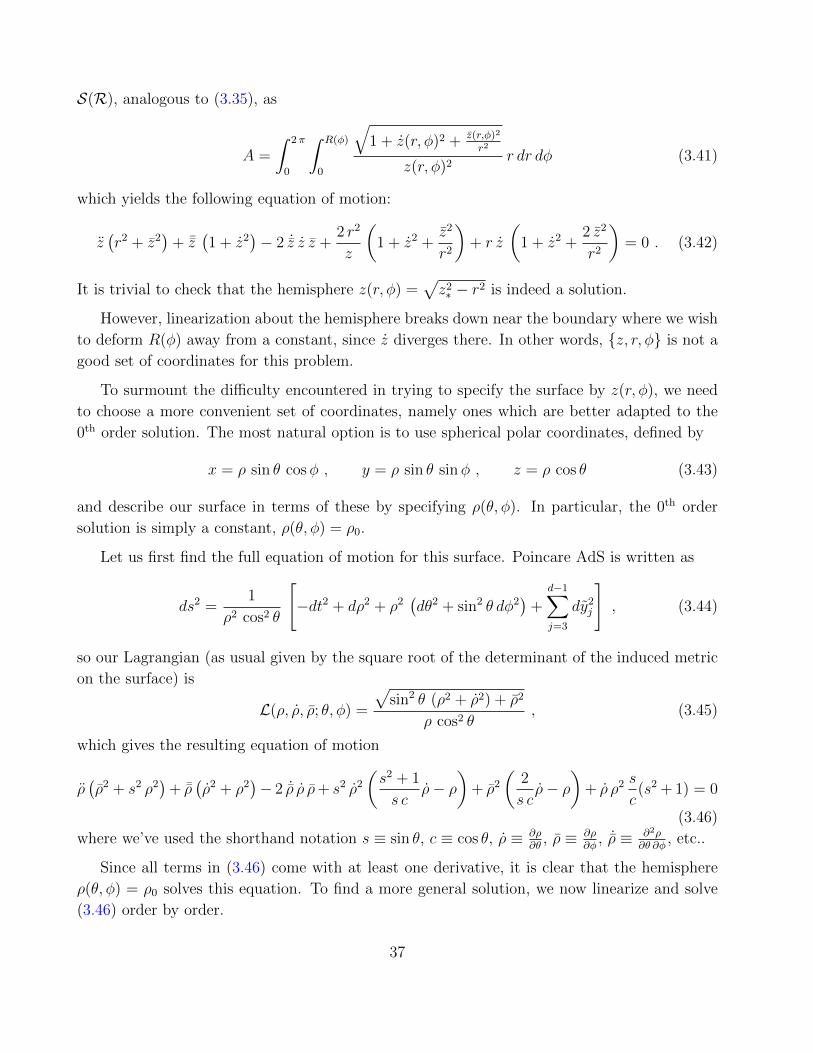
S(R), analogous to (3.35), as

A =

∫ 2π

0

∫ R(φ)

0

√1 + z(r, φ)2 + z(r,φ)2

r2

z(r, φ)2r dr dφ (3.41)

which yields the following equation of motion:

z(r2 + z2

)+ ¯z

(1 + z2

)− 2 ˙z z z +

2 r2

z

(1 + z2 +

z2

r2

)+ r z

(1 + z2 +

2 z2

r2

)= 0 . (3.42)

It is trivial to check that the hemisphere z(r, φ) =√z2∗ − r2 is indeed a solution.

However, linearization about the hemisphere breaks down near the boundary where we wish

to deform R(φ) away from a constant, since z diverges there. In other words, z, r, φ is not a

good set of coordinates for this problem.

To surmount the difficulty encountered in trying to specify the surface by z(r, φ), we need

to choose a more convenient set of coordinates, namely ones which are better adapted to the

0th order solution. The most natural option is to use spherical polar coordinates, defined by

x = ρ sin θ cosφ , y = ρ sin θ sinφ , z = ρ cos θ (3.43)

and describe our surface in terms of these by specifying ρ(θ, φ). In particular, the 0th order

solution is simply a constant, ρ(θ, φ) = ρ0.

Let us first find the full equation of motion for this surface. Poincare AdS is written as

ds2 =1

ρ2 cos2 θ

[−dt2 + dρ2 + ρ2

(dθ2 + sin2 θ dφ2

)+

d−1∑j=3

dy2j

], (3.44)

so our Lagrangian (as usual given by the square root of the determinant of the induced metric

on the surface) is

L(ρ, ρ, ρ; θ, φ) =

√sin2 θ (ρ2 + ρ2) + ρ2

ρ cos2 θ, (3.45)

which gives the resulting equation of motion

ρ(ρ2 + s2 ρ2

)+ ¯ρ

(ρ2 + ρ2

)− 2 ˙ρ ρ ρ+ s2 ρ2

(s2 + 1

s cρ− ρ

)+ ρ2

(2

s cρ− ρ

)+ ρ ρ2 s

c(s2 + 1) = 0

(3.46)

where we’ve used the shorthand notation s ≡ sin θ, c ≡ cos θ, ρ ≡ ∂ρ∂θ

, ρ ≡ ∂ρ∂φ

, ˙ρ ≡ ∂2ρ∂θ ∂φ

, etc..

Since all terms in (3.46) come with at least one derivative, it is clear that the hemisphere

ρ(θ, φ) = ρ0 solves this equation. To find a more general solution, we now linearize and solve

(3.46) order by order.

37

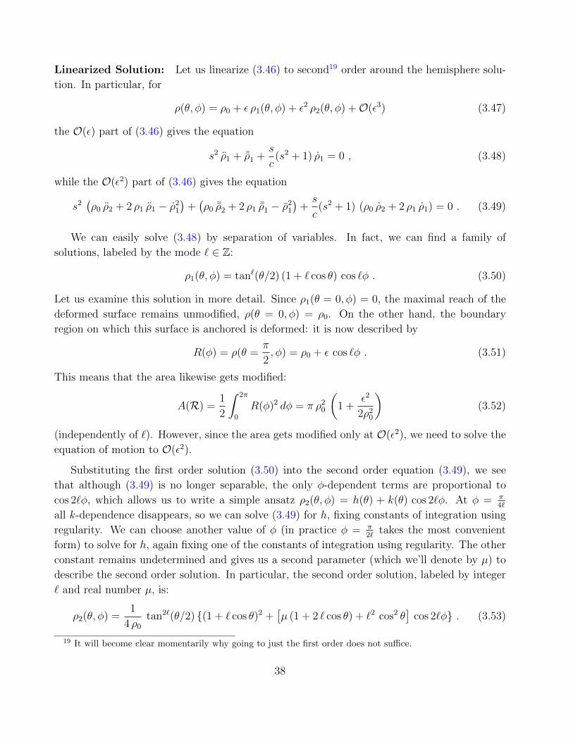
Linearized Solution: Let us linearize (3.46) to second19 order around the hemisphere solu-

tion. In particular, for

ρ(θ, φ) = ρ0 + ε ρ1(θ, φ) + ε2 ρ2(θ, φ) +O(ε3) (3.47)

the O(ε) part of (3.46) gives the equation

s2 ρ1 + ¯ρ1 +s

c(s2 + 1) ρ1 = 0 , (3.48)

while the O(ε2) part of (3.46) gives the equation

s2(ρ0 ρ2 + 2 ρ1 ρ1 − ρ2

1

)+(ρ0 ¯ρ2 + 2 ρ1 ¯ρ1 − ρ2

1

)+s

c(s2 + 1) (ρ0 ρ2 + 2 ρ1 ρ1) = 0 . (3.49)

We can easily solve (3.48) by separation of variables. In fact, we can find a family of

solutions, labeled by the mode ` ∈ Z:

ρ1(θ, φ) = tan`(θ/2) (1 + ` cos θ) cos `φ . (3.50)

Let us examine this solution in more detail. Since ρ1(θ = 0, φ) = 0, the maximal reach of the

deformed surface remains unmodified, ρ(θ = 0, φ) = ρ0. On the other hand, the boundary

region on which this surface is anchored is deformed: it is now described by

R(φ) = ρ(θ =π

2, φ) = ρ0 + ε cos `φ . (3.51)

This means that the area likewise gets modified:

A(R) =1

2

∫ 2π

0

R(φ)2 dφ = π ρ20

(1 +

ε2

2ρ20

)(3.52)

(independently of `). However, since the area gets modified only at O(ε2), we need to solve the

equation of motion to O(ε2).

Substituting the first order solution (3.50) into the second order equation (3.49), we see

that although (3.49) is no longer separable, the only φ-dependent terms are proportional to

cos 2`φ, which allows us to write a simple ansatz ρ2(θ, φ) = h(θ) + k(θ) cos 2`φ. At φ = π4`

all k-dependence disappears, so we can solve (3.49) for h, fixing constants of integration using

regularity. We can choose another value of φ (in practice φ = π2`

takes the most convenient

form) to solve for h, again fixing one of the constants of integration using regularity. The other

constant remains undetermined and gives us a second parameter (which we’ll denote by µ) to

describe the second order solution. In particular, the second order solution, labeled by integer

` and real number µ, is:

ρ2(θ, φ) =1

4 ρ0

tan2`(θ/2) (1 + ` cos θ)2 +[µ (1 + 2 ` cos θ) + `2 cos2 θ

]cos 2`φ . (3.53)

19 It will become clear momentarily why going to just the first order does not suffice.

38

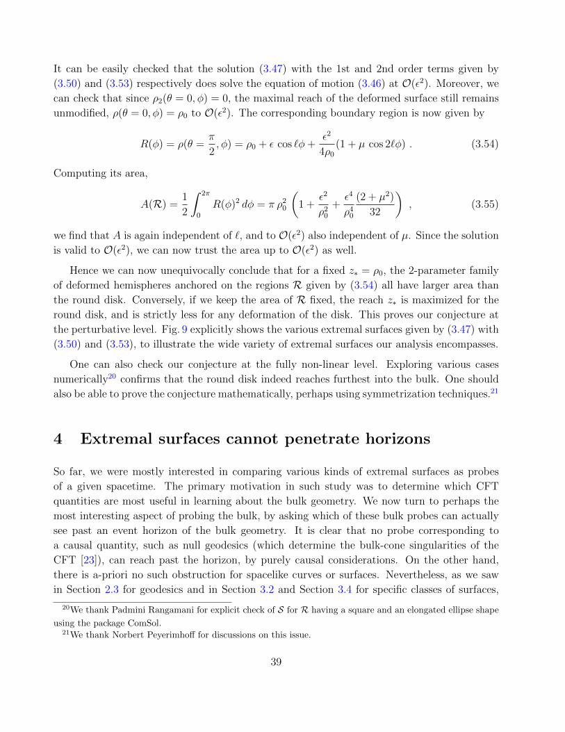
It can be easily checked that the solution (3.47) with the 1st and 2nd order terms given by

(3.50) and (3.53) respectively does solve the equation of motion (3.46) at O(ε2). Moreover, we

can check that since ρ2(θ = 0, φ) = 0, the maximal reach of the deformed surface still remains

unmodified, ρ(θ = 0, φ) = ρ0 to O(ε2). The corresponding boundary region is now given by

R(φ) = ρ(θ =π

2, φ) = ρ0 + ε cos `φ+

ε2

4ρ0

(1 + µ cos 2`φ) . (3.54)

Computing its area,

A(R) =1

2

∫ 2π

0

R(φ)2 dφ = π ρ20

(1 +

ε2

ρ20

+ε4

ρ40

(2 + µ2)

32

), (3.55)

we find that A is again independent of `, and to O(ε2) also independent of µ. Since the solution

is valid to O(ε2), we can now trust the area up to O(ε2) as well.

Hence we can now unequivocally conclude that for a fixed z∗ = ρ0, the 2-parameter family

of deformed hemispheres anchored on the regions R given by (3.54) all have larger area than

the round disk. Conversely, if we keep the area of R fixed, the reach z∗ is maximized for the

round disk, and is strictly less for any deformation of the disk. This proves our conjecture at

the perturbative level. Fig. 9 explicitly shows the various extremal surfaces given by (3.47) with

(3.50) and (3.53), to illustrate the wide variety of extremal surfaces our analysis encompasses.

One can also check our conjecture at the fully non-linear level. Exploring various cases

numerically20 confirms that the round disk indeed reaches furthest into the bulk. One should

also be able to prove the conjecture mathematically, perhaps using symmetrization techniques.21

4 Extremal surfaces cannot penetrate horizons

So far, we were mostly interested in comparing various kinds of extremal surfaces as probes

of a given spacetime. The primary motivation in such study was to determine which CFT

quantities are most useful in learning about the bulk geometry. We now turn to perhaps the

most interesting aspect of probing the bulk, by asking which of these bulk probes can actually

see past an event horizon of the bulk geometry. It is clear that no probe corresponding to

a causal quantity, such as null geodesics (which determine the bulk-cone singularities of the

CFT [23]), can reach past the horizon, by purely causal considerations. On the other hand,

there is a-priori no such obstruction for spacelike curves or surfaces. Nevertheless, as we saw

in Section 2.3 for geodesics and in Section 3.2 and Section 3.4 for specific classes of surfaces,

20We thank Padmini Rangamani for explicit check of S for R having a square and an elongated ellipse shape

using the package ComSol.21We thank Norbert Peyerimhoff for discussions on this issue.

39

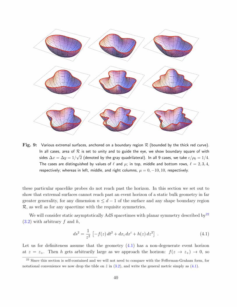
Fig. 9: Various extremal surfaces, anchored on a boundary region R (bounded by the thick red curve).

In all cases, area of R is set to unity and to guide the eye, we show boundary square of with

sides ∆x = ∆y = 1/√

2 (denoted by the gray quadrilateral). In all 9 cases, we take ε/ρ0 = 1/4.

The cases are distinguished by values of ` and µ; in top, middle and bottom rows, ` = 2, 3, 4,

respectively; whereas in left, middle, and right columns, µ = 0,−10, 10, respectively.

these particular spacelike probes do not reach past the horizon. In this section we set out to

show that extremal surfaces cannot reach past an event horizon of a static bulk geometry in far

greater generality, for any dimension n ≤ d− 1 of the surface and any shape boundary region

R, as well as for any spacetime with the requisite symmetries.

We will consider static asymptotically AdS spacetimes with planar symmetry described by22

(3.2) with arbitrary f and h,

ds2 =1

z2

[−f(z) dt2 + dxi dx

i + h(z) dz2]. (4.1)

Let us for definiteness assume that the geometry (4.1) has a non-degenerate event horizon

at z = z+. Then h gets arbitrarily large as we approach the horizon: f(z → z+) → 0, so

22 Since this section is self-contained and we will not need to compare with the Fefferman-Graham form, for

notational convenience we now drop the tilde on z in (3.2), and write the general metric simply as (4.1).

40

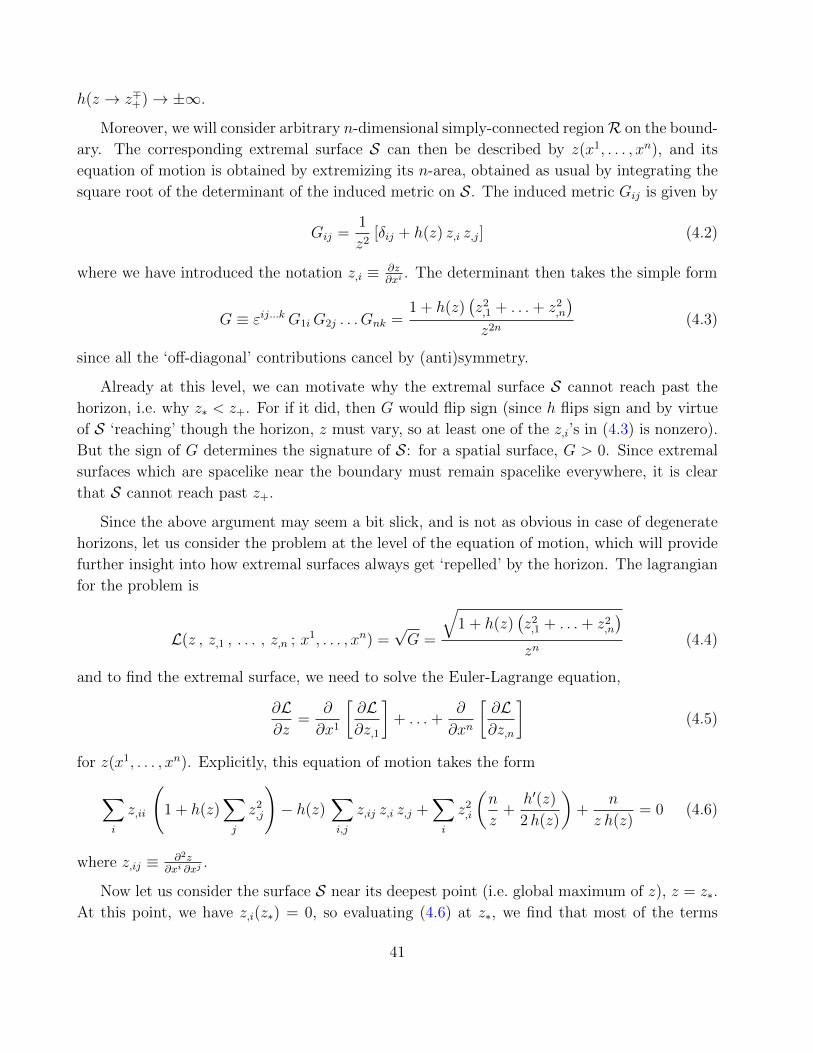
h(z → z∓+)→ ±∞.

Moreover, we will consider arbitrary n-dimensional simply-connected regionR on the bound-

ary. The corresponding extremal surface S can then be described by z(x1, . . . , xn), and its

equation of motion is obtained by extremizing its n-area, obtained as usual by integrating the

square root of the determinant of the induced metric on S. The induced metric Gij is given by

Gij =1

z2[δij + h(z) z,i z,j] (4.2)

where we have introduced the notation z,i ≡ ∂z∂xi

. The determinant then takes the simple form

G ≡ εij...kG1iG2j . . . Gnk =1 + h(z)

(z2,1 + . . .+ z2

,n

)z2n

(4.3)

since all the ‘off-diagonal’ contributions cancel by (anti)symmetry.

Already at this level, we can motivate why the extremal surface S cannot reach past the

horizon, i.e. why z∗ < z+. For if it did, then G would flip sign (since h flips sign and by virtue

of S ‘reaching’ though the horizon, z must vary, so at least one of the z,i’s in (4.3) is nonzero).

But the sign of G determines the signature of S: for a spatial surface, G > 0. Since extremal

surfaces which are spacelike near the boundary must remain spacelike everywhere, it is clear

that S cannot reach past z+.

Since the above argument may seem a bit slick, and is not as obvious in case of degenerate

horizons, let us consider the problem at the level of the equation of motion, which will provide

further insight into how extremal surfaces always get ‘repelled’ by the horizon. The lagrangian

for the problem is

L(z , z,1 , . . . , z,n ; x1, . . . , xn) =√G =

√1 + h(z)

(z2,1 + . . .+ z2

,n

)zn

(4.4)

and to find the extremal surface, we need to solve the Euler-Lagrange equation,

∂L∂z

=∂

∂x1

[∂L∂z,1

]+ . . .+

∂

∂xn

[∂L∂z,n

](4.5)

for z(x1, . . . , xn). Explicitly, this equation of motion takes the form

∑i

z,ii

(1 + h(z)

∑j

z2,j

)− h(z)

∑i,j

z,ij z,i z,j +∑i

z2,i

(n

z+

h′(z)

2h(z)

)+

n

z h(z)= 0 (4.6)

where z,ij ≡ ∂2z∂xi ∂xj

.

Now let us consider the surface S near its deepest point (i.e. global maximum of z), z = z∗.

At this point, we have z,i(z∗) = 0, so evaluating (4.6) at z∗, we find that most of the terms

41

vanish and we are left with ∑i

z,ii +n

z h(z)= 0 at z = z∗ . (4.7)

In order for z = z∗ to be a maximum, we additionally need z,ii(z∗) < 0. This forces h(z∗) > 0,

i.e., z∗ < z+. In other words, the maximal reach of S cannot not extend all the way to the

horizon, which shows that extremal surfaces cannot penetrate horizons.

Moreover, the closer S approaches to the horizon, the smaller magnitude z,ii may be whilst

satisfying (4.7), so the flatter S has to get near its tip – but that in turn means that the larger

the corresponding boundary region R has to be. As the tip of the extremal surface approaches

the horizon, the extent of the boundary region R spanned by ∂S diverges. We now see that

this argument in fact generalizes to any horizon, including the degenerate case.

5 Discussion

In this paper we have explored the capacity of various CFT probes for encoding the bulk geom-

etry. The probes under consideration were those represented by specific geometric quantities,

namely extremal surfaces, in the bulk. Since the position of an extremal surface is determined

by the bulk geometry and the boundary conditions, one may hope to invert this information to

learn about the bulk geometry using the CFT data. In particular, using a family of boundary

conditions and some characteristic of the surface such as its volume, we would hope to extract

the bulk metric. This has been successfully used in several contexts in the past, as reviewed in

[13].

The goal of the present work was not to perform such an extraction, but rather to explore its

limitations. In particular, one may extract the bulk geometry by extremal surface probes only

in a region of spacetime which is accessible to such extremal surfaces. Considering which types

of surfaces are a-priori (i.e. before knowing the bulk geometry) most suitable for reaching the

largest region of the bulk, then allows us to focus on the most convenient CFT data to be used

for our extraction. Of course, there is a limitation to how far one can get while maintaining full

generality. We have therefore focused on a case where the bulk geometry has certain symmetries

which can be easily specified within the CFT.

In particular, if the CFT state is static and homogeneous, the bulk geometry likewise in-

herits these properties; so in the present work, we have considered static spacetimes which

were homogeneous in the boundary directions. We have considered two classes of boundary

background spacetimes on which the field theory lives: in Section 2 we considered CFT on Ein-

stein static universe relevant for spherically symmetric asymptotically globally AdS spacetimes

(2.1), while in Section 3 and Section 4 we turned to CFT on Minkowski spacetime, pertaining

42

to translationally invariant asymptotically Poincare AdS bulk geometries (3.2).

Apart from rendering the calculations tractable, this restriction had the advantage of en-

abling us to characterize and compare the reach of the various probes in a simple geometrical

fashion. In the former case of global AdS we defined the radial coordinate r by proper area

of the d − 1 spheres as usual, and characterized the reach of extremal surfaces – in that case

geodesics – by the minimum value r∗ that this coordinate achieves along a given geodesic. In

the latter case, we used Fefferman-Graham coordinate z (related to proper length along radial

geodesics) and characterized the reach of extremal surfaces by its maximal value z∗ attained

along such surfaces.

Although one could relax our symmetry constraints it would complicate the comparisons.

For example, in a spatially-varying geometry, one semi-natural way to define z∗ purely geo-

metrically would be to use affine parameter along ingoing geodesics emanating orthogonally to

the boundary fluid velocity, analogously to the set-up used in the fluid/gravity correspondence

[46]; however unless the spacetime varied slowly enough in the boundary directions, the caus-

tics where such coordinate system breaks down might occur already within the reach of the

extremal surfaces. While by no means insurmountable, this complication would nevertheless

hinder us in making fully general statements.

On the other hand, it would be very interesting to explore the consequences of relaxing the

imposed symmetries. For instance, one could explore whether the extremal surfaces deform

in some intriguing fashion. Of particular interest would be to introduce some non-trivial time

dependence into our spacetime. As mentioned below, this can even invalidate the conclusions

reached in the previous section by allowing extremal surfaces to extend through an event

horizon. One convenient set-up wherein one could make definitive statements in absence of any

symmetries is the fluid/gravity regime [46], valid when the geometry varies sufficiently slowly

in the boundary directions. This is unfortunately unlikely to produce the type of evolution

needed to probe past event horizons, but nevertheless would allow us to gain further insight

into the effects that time dependence can produce.

A much milder form of relaxing staticity was explored in [34] by considering stationary

geometries. While such geometries are still time-translation invariant, they are not time-reversal

invariant, so extremal surfaces need no longer lie at constant-t slice. For example, the set of

all spacelike geodesics anchored at t = 0 on the boundary of rotating BTZ spacetime spans not

a single spacelike slice of the bulk but rather a co-dimension 0 spacetime volume with finite

time extent. This suggests the intriguing possibility that the knowledge of the CFT data at a

single time allows us to directly extract the bulk geometry over a range of bulk times. These

observations demonstrate that relaxing the symmetries allows a richer set of possibilities, which

we leave for future explorations.

Returning to the static and homogeneous configurations discussed above, specified by two

43

arbitrary functions of one variable (the bulk radial coordinate), we now summarize our main

results.

In Section 2 we explored ‘probe’ geodesics, characterized by both endpoints anchored on

the (same) AdS boundary. While null geodesics might represent the easiest CFT probes to use

in terms of ready availability of the CFT data, we saw that they are not the best probes for

accessing the largest possible region of spacetime. In particular, for any null geodesic, there

always exists a spacelike one which admits smaller r∗. This has implications for decoding the

spacetime if we restrict the CFT region on which we’re allowed to specify the CFT data, or

if the bulk spacetime is causally nontrivial (or admits null circular orbits). In such cases, the

‘optimal’ geodesics to probe the spatial geometry turn out to be the E = 0 spacelike ones23

since these not only have ∆t = 0, but also minimize r∗ at fixed ∆ϕ.

In the causally interesting case describing a black hole, we showed that probe geodesics

cannot reach past the horizon, but that there is a family of spacelike geodesics which can probe

arbitrarily near the horizon; these correspond to E = 0 and L → (r+)+. Such geodesics have

large ∆ϕ and correspondingly large Lreg, because they orbit the black hole in the vicinity of

the horizon many times. Imposing finite upper bound on ∆ϕ or Lreg restricts r∗ to be finitely

larger than r+, though we saw that for typical examples this is not too severe. Null geodesics,

on the other hand, can typically probe to only O(r+) distance from the horizon.

Given that E = 0 geodesics represented the best 1-dimensional probes, in the remaining

sections we restricted attention to extremal surfaces anchored on the boundary at constant

time. For static geometries this implies that the entire surface lies at constant bulk time, and

is therefore insensitive to gtt in the bulk metric. This leaves one arbitrary function of the bulk

radial coordinate, characterizing the spatial geometry of the bulk, which we can try to extract

via such extremal surfaces. Section 3 explored which extremal surfaces are the best probes of

this spatial geometry. Unlike the geodesic case where we only had a single parameter, L, at our

disposal, we now have a far richer set of attributes by which to characterize an extremal surface

S. Apart from the dimensionality n, we can freely specify the boundary region R defining the

surface S. In Section 3 we examined how these attributes affect the behaviour of S.

One theme which we explored was how does the dimensionality n of the extremal surface

affect its reach z∗. In Section 3.1 we considered ‘strip’ regions R with a given thickness ∆x,

observing that higher-dimensional surfaces appear to be better probes of the bulk geometry,

in the sense that z∗/∆x grows with n in pure AdS. To convince ourselves that this is not an

artifact of pure AdS geometry, in Section 3.2 we extended the result to more general asymptot-

ically AdS spacetimes. However, as we saw, this question needs to be specified more carefully,

since we can’t directly compare quantities of different dimensions. In particular, the strip has

infinite extent in the remaining n−1 directions, so that higher-dimensional regions utilize much

23 These are however insensitive to the time component of the metric as they lie at constant t.

44

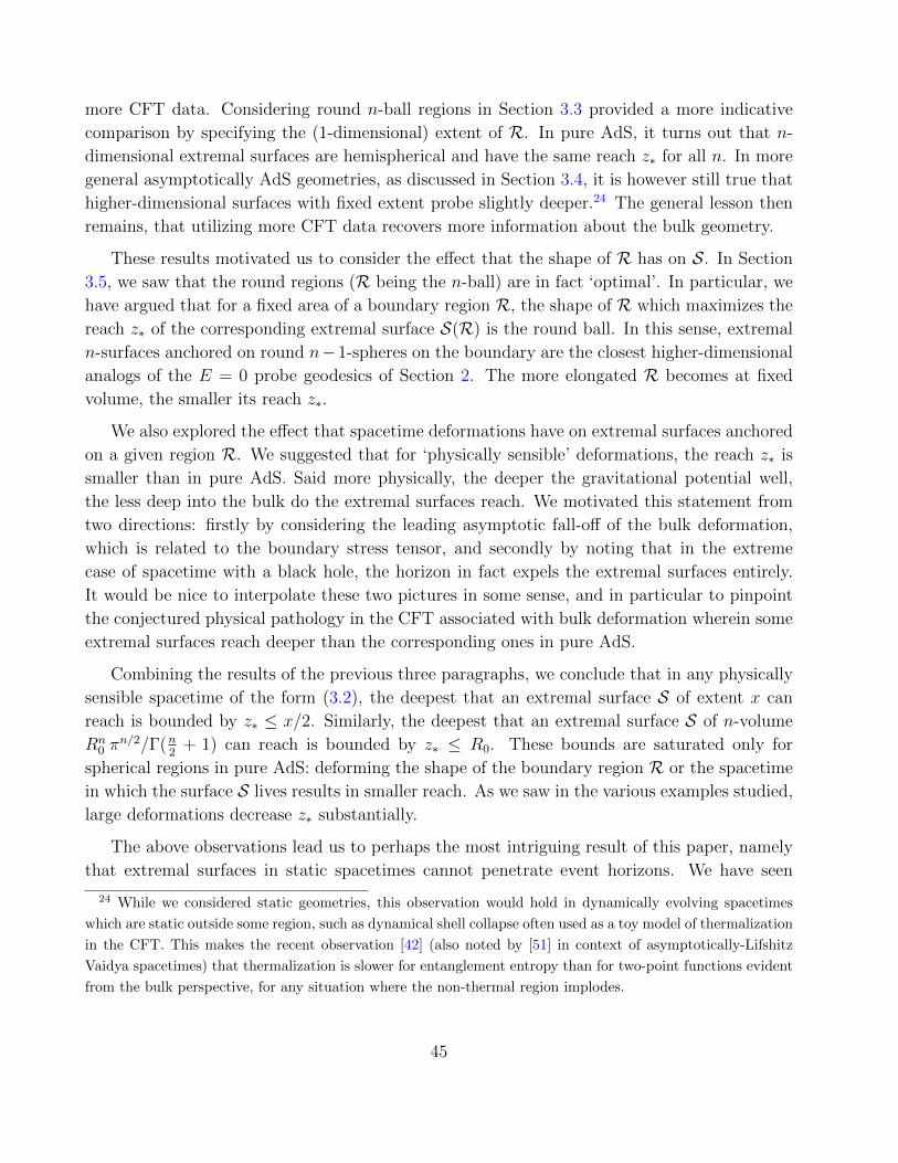
more CFT data. Considering round n-ball regions in Section 3.3 provided a more indicative

comparison by specifying the (1-dimensional) extent of R. In pure AdS, it turns out that n-

dimensional extremal surfaces are hemispherical and have the same reach z∗ for all n. In more

general asymptotically AdS geometries, as discussed in Section 3.4, it is however still true that

higher-dimensional surfaces with fixed extent probe slightly deeper.24 The general lesson then

remains, that utilizing more CFT data recovers more information about the bulk geometry.

These results motivated us to consider the effect that the shape of R has on S. In Section

3.5, we saw that the round regions (R being the n-ball) are in fact ‘optimal’. In particular, we

have argued that for a fixed area of a boundary region R, the shape of R which maximizes the

reach z∗ of the corresponding extremal surface S(R) is the round ball. In this sense, extremal

n-surfaces anchored on round n−1-spheres on the boundary are the closest higher-dimensional

analogs of the E = 0 probe geodesics of Section 2. The more elongated R becomes at fixed

volume, the smaller its reach z∗.

We also explored the effect that spacetime deformations have on extremal surfaces anchored

on a given region R. We suggested that for ‘physically sensible’ deformations, the reach z∗ is

smaller than in pure AdS. Said more physically, the deeper the gravitational potential well,

the less deep into the bulk do the extremal surfaces reach. We motivated this statement from

two directions: firstly by considering the leading asymptotic fall-off of the bulk deformation,

which is related to the boundary stress tensor, and secondly by noting that in the extreme

case of spacetime with a black hole, the horizon in fact expels the extremal surfaces entirely.

It would be nice to interpolate these two pictures in some sense, and in particular to pinpoint

the conjectured physical pathology in the CFT associated with bulk deformation wherein some

extremal surfaces reach deeper than the corresponding ones in pure AdS.

Combining the results of the previous three paragraphs, we conclude that in any physically

sensible spacetime of the form (3.2), the deepest that an extremal surface S of extent x can

reach is bounded by z∗ ≤ x/2. Similarly, the deepest that an extremal surface S of n-volume

Rn0 π

n/2/Γ(n2

+ 1) can reach is bounded by z∗ ≤ R0. These bounds are saturated only for

spherical regions in pure AdS: deforming the shape of the boundary region R or the spacetime

in which the surface S lives results in smaller reach. As we saw in the various examples studied,

large deformations decrease z∗ substantially.

The above observations lead us to perhaps the most intriguing result of this paper, namely

that extremal surfaces in static spacetimes cannot penetrate event horizons. We have seen

24 While we considered static geometries, this observation would hold in dynamically evolving spacetimes

which are static outside some region, such as dynamical shell collapse often used as a toy model of thermalization

in the CFT. This makes the recent observation [42] (also noted by [51] in context of asymptotically-Lifshitz

Vaidya spacetimes) that thermalization is slower for entanglement entropy than for two-point functions evident

from the bulk perspective, for any situation where the non-thermal region implodes.

45

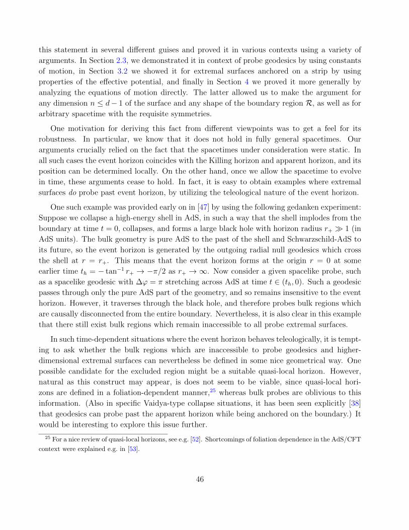
this statement in several different guises and proved it in various contexts using a variety of

arguments. In Section 2.3, we demonstrated it in context of probe geodesics by using constants

of motion, in Section 3.2 we showed it for extremal surfaces anchored on a strip by using

properties of the effective potential, and finally in Section 4 we proved it more generally by

analyzing the equations of motion directly. The latter allowed us to make the argument for

any dimension n ≤ d− 1 of the surface and any shape of the boundary region R, as well as for

arbitrary spacetime with the requisite symmetries.

One motivation for deriving this fact from different viewpoints was to get a feel for its

robustness. In particular, we know that it does not hold in fully general spacetimes. Our

arguments crucially relied on the fact that the spacetimes under consideration were static. In

all such cases the event horizon coincides with the Killing horizon and apparent horizon, and its

position can be determined locally. On the other hand, once we allow the spacetime to evolve

in time, these arguments cease to hold. In fact, it is easy to obtain examples where extremal

surfaces do probe past event horizon, by utilizing the teleological nature of the event horizon.

One such example was provided early on in [47] by using the following gedanken experiment:

Suppose we collapse a high-energy shell in AdS, in such a way that the shell implodes from the

boundary at time t = 0, collapses, and forms a large black hole with horizon radius r+ 1 (in

AdS units). The bulk geometry is pure AdS to the past of the shell and Schwarzschild-AdS to

its future, so the event horizon is generated by the outgoing radial null geodesics which cross

the shell at r = r+. This means that the event horizon forms at the origin r = 0 at some

earlier time th = − tan−1 r+ → −π/2 as r+ → ∞. Now consider a given spacelike probe, such

as a spacelike geodesic with ∆ϕ = π stretching across AdS at time t ∈ (th, 0). Such a geodesic

passes through only the pure AdS part of the geometry, and so remains insensitive to the event

horizon. However, it traverses through the black hole, and therefore probes bulk regions which

are causally disconnected from the entire boundary. Nevertheless, it is also clear in this example

that there still exist bulk regions which remain inaccessible to all probe extremal surfaces.

In such time-dependent situations where the event horizon behaves teleologically, it is tempt-

ing to ask whether the bulk regions which are inaccessible to probe geodesics and higher-

dimensional extremal surfaces can nevertheless be defined in some nice geometrical way. One

possible candidate for the excluded region might be a suitable quasi-local horizon. However,

natural as this construct may appear, is does not seem to be viable, since quasi-local hori-

zons are defined in a foliation-dependent manner,25 whereas bulk probes are oblivious to this

information. (Also in specific Vaidya-type collapse situations, it has been seen explicitly [38]

that geodesics can probe past the apparent horizon while being anchored on the boundary.) It

would be interesting to explore this issue further.

25 For a nice review of quasi-local horizons, see e.g. [52]. Shortcomings of foliation dependence in the AdS/CFT

context were explained e.g. in [53].

46

Acknowledgements

It is a pleasure to thank Roberto Emparan, Gary Horowitz, Don Marolf, Joe Polchinski, and

Mukund Rangamani for many stimulating discussions during various stages of this project. I

also thank Hong Liu, Mukund Rangamani, and Tadashi Takayanagi for collaborations which

inspired the present exploration. This work was supported in part by an STFC Consolidated

Grant ST/J000426/1.

References

[1] J. M. Maldacena, “The large N limit of superconformal field theories and supergravity,”

Adv. Theor. Math. Phys. 2 (1998) 231–252, arXiv:hep-th/9711200.

[2] T. Banks, M. R. Douglas, G. T. Horowitz, and E. J. Martinec, “AdS dynamics from

conformal field theory,” arXiv:hep-th/9808016 [hep-th].

[3] J. Polchinski, “S matrices from AdS space-time,” arXiv:hep-th/9901076 [hep-th].

[4] L. Susskind, “Holography in the flat space limit,” arXiv:hep-th/9901079 [hep-th].

[5] S. B. Giddings, “Flat space scattering and bulk locality in the AdS / CFT

correspondence,” Phys.Rev. D61 (2000) 106008, arXiv:hep-th/9907129 [hep-th].

[6] G. T. Horowitz and V. E. Hubeny, “CFT description of small objects in AdS,” JHEP 10

(2000) 027, arXiv:hep-th/0009051.

[7] A. Hamilton, D. N. Kabat, G. Lifschytz, and D. A. Lowe, “Local bulk operators in

AdS/CFT: A Boundary view of horizons and locality,” Phys.Rev. D73 (2006) 086003,

arXiv:hep-th/0506118 [hep-th].

[8] M. Gary and S. B. Giddings, “The Flat space S-matrix from the AdS/CFT

correspondence?,” Phys.Rev. D80 (2009) 046008, arXiv:0904.3544 [hep-th].

[9] I. Heemskerk, J. Penedones, J. Polchinski, and J. Sully, “Holography from Conformal

Field Theory,” JHEP 10 (2009) 079, arXiv:0907.0151 [hep-th].

[10] D. Kabat, G. Lifschytz, and D. A. Lowe, “Constructing local bulk observables in

interacting AdS/CFT,” Phys.Rev. D83 (2011) 106009, arXiv:1102.2910 [hep-th].

[11] A. Fitzpatrick and J. Kaplan, “Scattering States in AdS/CFT,” arXiv:1104.2597

[hep-th].

47

[12] I. Heemskerk, D. Marolf, and J. Polchinski, “Bulk and Transhorizon Measurements in

AdS/CFT,” arXiv:1201.3664 [hep-th].

[13] V. E. Hubeny and M. Rangamani, “A Holographic view on physics out of equilibrium,”

Adv.High Energy Phys. 2010 (2010) 297916, arXiv:1006.3675 [hep-th].

[14] L. Fidkowski, V. Hubeny, M. Kleban, and S. Shenker, “The black hole singularity in

AdS/CFT,” JHEP 02 (2004) 014, arXiv:hep-th/0306170.

[15] G. Festuccia and H. Liu, “Excursions beyond the horizon: Black hole singularities in

Yang-Mills theories. I,” JHEP 04 (2006) 044, arXiv:hep-th/0506202.

[16] V. Balasubramanian and S. F. Ross, “Holographic particle detection,” Phys. Rev. D61

(2000) 044007, arXiv:hep-th/9906226.

[17] J. Louko, D. Marolf, and S. F. Ross, “On geodesic propagators and black hole

holography,” Phys. Rev. D62 (2000) 044041, arXiv:hep-th/0002111.

[18] P. Kraus, H. Ooguri, and S. Shenker, “Inside the horizon with AdS/CFT,” Phys. Rev.

D67 (2003) 124022, arXiv:hep-th/0212277.

[19] V. Balasubramanian et al., “Typicality versus thermality: An analytic distinction,” Gen.

Rel. Grav. 40 (2008) 1863–1890, arXiv:hep-th/0701122.

[20] S. D. Mathur, “The fuzzball proposal for black holes: An elementary review,” Fortsch.

Phys. 53 (2005) 793–827, arXiv:hep-th/0502050.

[21] K. Skenderis and M. Taylor, “The fuzzball proposal for black holes,” Phys. Rept. 467

(2008) 117–171, arXiv:0804.0552 [hep-th].

[22] B. Freivogel, V. Hubeny, A. Maloney, R. Myers, M. Rangamani, and S. Shenker,

“Inflation in AdS/CFT,” JHEP 03 (2006) 007, arXiv:hep-th/0510046.

[23] V. E. Hubeny, H. Liu, and M. Rangamani, “Bulk-cone singularities & signatures of

horizon formation in AdS/CFT,” JHEP 01 (2007) 009, arXiv:hep-th/0610041.

[24] S. Gao and R. M. Wald, “Theorems on gravitational time delay and related issues,”

Class. Quant. Grav. 17 (2000) 4999–5008, arXiv:gr-qc/0007021.

[25] J. Erdmenger, C. Hoyos, and S. Lin, “Time Singularities of Correlators from Dirichlet

Conditions in AdS/CFT,” arXiv:1112.1963 [hep-th]. 29 pages, 3 figures.

[26] I. Amado and C. Hoyos-Badajoz, “AdS black holes as reflecting cavities,” JHEP 0809

(2008) 118, arXiv:0807.2337 [hep-th].

48

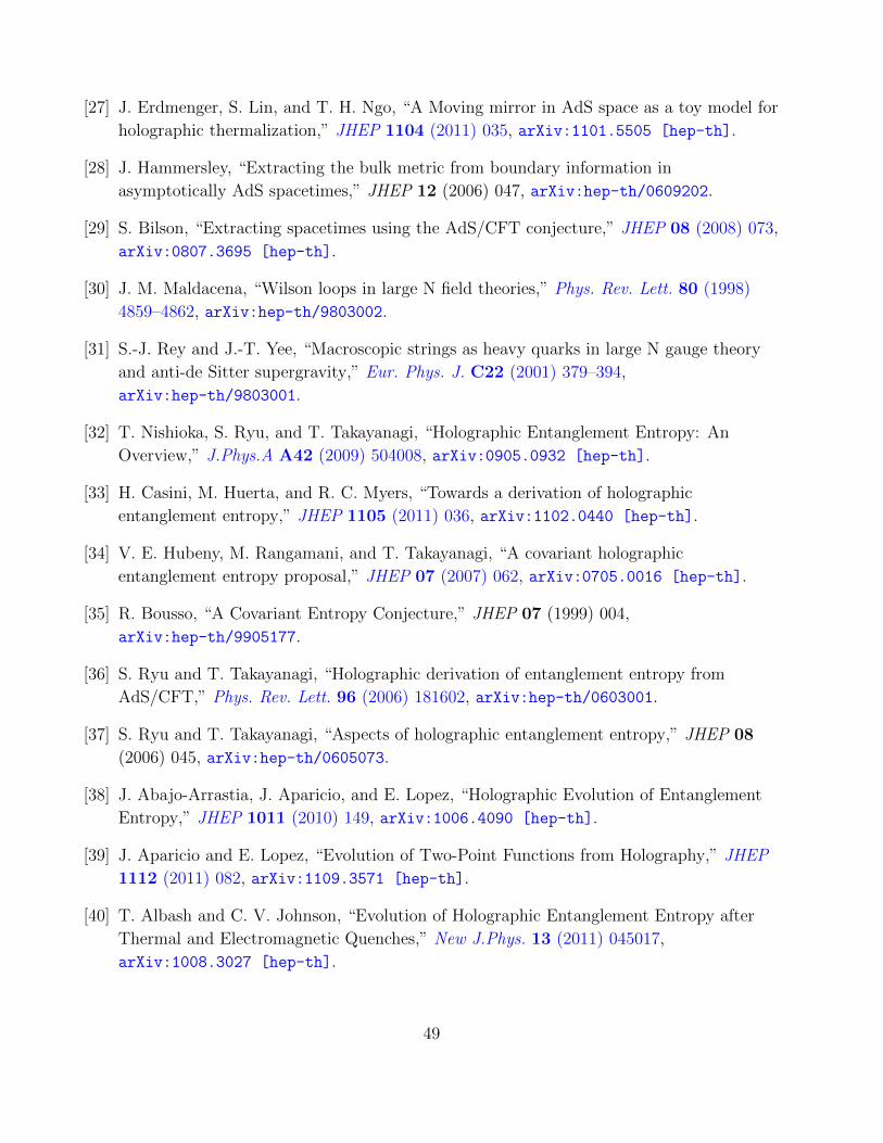
[27] J. Erdmenger, S. Lin, and T. H. Ngo, “A Moving mirror in AdS space as a toy model for

holographic thermalization,” JHEP 1104 (2011) 035, arXiv:1101.5505 [hep-th].

[28] J. Hammersley, “Extracting the bulk metric from boundary information in

asymptotically AdS spacetimes,” JHEP 12 (2006) 047, arXiv:hep-th/0609202.

[29] S. Bilson, “Extracting spacetimes using the AdS/CFT conjecture,” JHEP 08 (2008) 073,

arXiv:0807.3695 [hep-th].

[30] J. M. Maldacena, “Wilson loops in large N field theories,” Phys. Rev. Lett. 80 (1998)

4859–4862, arXiv:hep-th/9803002.

[31] S.-J. Rey and J.-T. Yee, “Macroscopic strings as heavy quarks in large N gauge theory

and anti-de Sitter supergravity,” Eur. Phys. J. C22 (2001) 379–394,

arXiv:hep-th/9803001.

[32] T. Nishioka, S. Ryu, and T. Takayanagi, “Holographic Entanglement Entropy: An

Overview,” J.Phys.A A42 (2009) 504008, arXiv:0905.0932 [hep-th].

[33] H. Casini, M. Huerta, and R. C. Myers, “Towards a derivation of holographic

entanglement entropy,” JHEP 1105 (2011) 036, arXiv:1102.0440 [hep-th].

[34] V. E. Hubeny, M. Rangamani, and T. Takayanagi, “A covariant holographic

entanglement entropy proposal,” JHEP 07 (2007) 062, arXiv:0705.0016 [hep-th].

[35] R. Bousso, “A Covariant Entropy Conjecture,” JHEP 07 (1999) 004,

arXiv:hep-th/9905177.

[36] S. Ryu and T. Takayanagi, “Holographic derivation of entanglement entropy from

AdS/CFT,” Phys. Rev. Lett. 96 (2006) 181602, arXiv:hep-th/0603001.

[37] S. Ryu and T. Takayanagi, “Aspects of holographic entanglement entropy,” JHEP 08

(2006) 045, arXiv:hep-th/0605073.

[38] J. Abajo-Arrastia, J. Aparicio, and E. Lopez, “Holographic Evolution of Entanglement

Entropy,” JHEP 1011 (2010) 149, arXiv:1006.4090 [hep-th].

[39] J. Aparicio and E. Lopez, “Evolution of Two-Point Functions from Holography,” JHEP

1112 (2011) 082, arXiv:1109.3571 [hep-th].

[40] T. Albash and C. V. Johnson, “Evolution of Holographic Entanglement Entropy after

Thermal and Electromagnetic Quenches,” New J.Phys. 13 (2011) 045017,

arXiv:1008.3027 [hep-th].

49

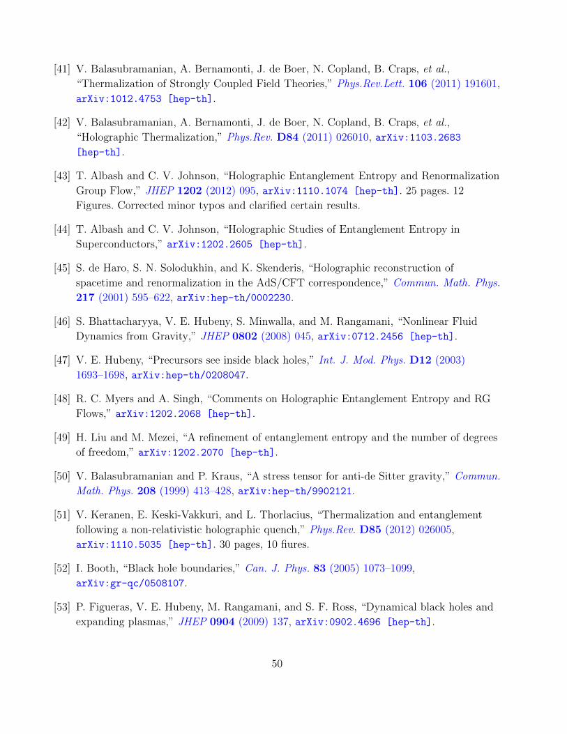
[41] V. Balasubramanian, A. Bernamonti, J. de Boer, N. Copland, B. Craps, et al.,

“Thermalization of Strongly Coupled Field Theories,” Phys.Rev.Lett. 106 (2011) 191601,

arXiv:1012.4753 [hep-th].

[42] V. Balasubramanian, A. Bernamonti, J. de Boer, N. Copland, B. Craps, et al.,

“Holographic Thermalization,” Phys.Rev. D84 (2011) 026010, arXiv:1103.2683

[hep-th].

[43] T. Albash and C. V. Johnson, “Holographic Entanglement Entropy and Renormalization

Group Flow,” JHEP 1202 (2012) 095, arXiv:1110.1074 [hep-th]. 25 pages. 12

Figures. Corrected minor typos and clarified certain results.

[44] T. Albash and C. V. Johnson, “Holographic Studies of Entanglement Entropy in

Superconductors,” arXiv:1202.2605 [hep-th].

[45] S. de Haro, S. N. Solodukhin, and K. Skenderis, “Holographic reconstruction of

spacetime and renormalization in the AdS/CFT correspondence,” Commun. Math. Phys.

217 (2001) 595–622, arXiv:hep-th/0002230.

[46] S. Bhattacharyya, V. E. Hubeny, S. Minwalla, and M. Rangamani, “Nonlinear Fluid

Dynamics from Gravity,” JHEP 0802 (2008) 045, arXiv:0712.2456 [hep-th].

[47] V. E. Hubeny, “Precursors see inside black holes,” Int. J. Mod. Phys. D12 (2003)

1693–1698, arXiv:hep-th/0208047.

[48] R. C. Myers and A. Singh, “Comments on Holographic Entanglement Entropy and RG

Flows,” arXiv:1202.2068 [hep-th].

[49] H. Liu and M. Mezei, “A refinement of entanglement entropy and the number of degrees

of freedom,” arXiv:1202.2070 [hep-th].

[50] V. Balasubramanian and P. Kraus, “A stress tensor for anti-de Sitter gravity,” Commun.

Math. Phys. 208 (1999) 413–428, arXiv:hep-th/9902121.

[51] V. Keranen, E. Keski-Vakkuri, and L. Thorlacius, “Thermalization and entanglement

following a non-relativistic holographic quench,” Phys.Rev. D85 (2012) 026005,

arXiv:1110.5035 [hep-th]. 30 pages, 10 fiures.

[52] I. Booth, “Black hole boundaries,” Can. J. Phys. 83 (2005) 1073–1099,

arXiv:gr-qc/0508107.

[53] P. Figueras, V. E. Hubeny, M. Rangamani, and S. F. Ross, “Dynamical black holes and

expanding plasmas,” JHEP 0904 (2009) 137, arXiv:0902.4696 [hep-th].

50