Linköping Studies in Science and Technology Dissertations No.104

A NEWTON METHOD FOR SOLVING NON-LINEAR

OPTIMAL CONTROL PROBLEMS WITH GENERAL CONSTRAINTS

Henrik Jonson

Institutionen för Systemteknik

Linköpings Tekniska Högskola

Linköping 1983

ISBN 91-7372-718·0 JSSN 0345-7524

Prinlcd in Sweden by VTT-G raliskn, Vimmerby 1983

ABSTRACT Optimal eon tro! of general dynamic systems under realistic constraints on inputsignals a nd state variables is an important problem area in control theory. Many practical control problems can be formulated as optimization tasks,and this leads toasignificantdemand for efficient numerical solution algorithms.

Several such algorithms have been developed, and they are typically derived from a dynamic programming view point. ln this thesis a differentapproach is taken. The discrete­time dynamic optimization problem is fomrnJated as a static one, witb the inputs as free variables. Newton's approach to solving such a problem with constraints, also known as Wilson's method, is then consistently pursued, and a algorithm is developed that isa true Newton algorithm for the problem, at the same time as the inherentstructure is utilized for efficient calculations. An advantage witb such an approacb is that global and local conver­gence properties can be studied in a familiar framework.

The algorithm is tested on several examples and comparisons to other algorithms are carried out. T hese show that the Newton algorithm perfonns well and is competitive with other methods. It handles state variable constraints in a directand efficient manner, and its practical convergence properties are robust

A general algorithm for !arge scale static problems is also developed in the thesis, and it is tested on a problem with load distribution in an electrical power network.

ACKNOWLEDGEMENTS

I would like to express my deep gratitude to Professor Lennart

Ljung and my supervisor Torkel Glad for their guidance and

encouragement.

I also thank all my other friends and colleagues at the

Automatic Control group in Linköping for a pleasant atmosphere.

Specially

Bengt Bengtsson for proofreading

Ulla Salaneck for her patience when typing this manuscript,

Marianne Anse-Lundberg for drawing the figures.

My parents, relatives and friends for understanding and

support.

This research has been supported by the Swedish Institute of

Applied Mathemethics (ITM), which is hereby acknowledged.

CONTENTS Page

l.

2.

3.

4.

5.

6

7.

INTRODUCTION

1.1 Notations

OPTIMIZATION PROBLEMS AND OPTIMIZATION ALGORITHMS

SOLVING SPARSE QUADRATIC SUBPROBLEMS

3.1 Introduction

3.2

3.3

3 . 4

3. 5

An algorithm for solving quadratic problems

How to utilize the sparsity

Updating algorithms for t he A matrix

Positive definiteness of the A matrix

NONLINEAR OPTIMAL CONTROL PROBLEMS

4.1 Problem definition

4. 2

4. 3

Optimal control methods

Newton ' s method for optimal control problems

4.3 . 1 Derivation of the quadratic subproblem:

the case of no constraints

9

11

15

25

25 26

28

31

34

37

37

38

39

40

4 . 3 . 2 Derivation of the quadratic subproblem : 51

the case of one constraint .

4.3.3 Derivation of the quadratic subproblem: 56

the case of several constraints

4.4 Summary

ON THE CONSTRAINED LINEAR QUADRATIC

5 . 1 Introduction

5 . 2 Assumption Al in the CLQ ca se

5.3 Assumption A2 in the CLQ ca se.

5.4 Factorization and the Riccati

5.5 Inequality constraints

REGULARIZATION ISSUES

6.1 Introduction

6 . 2

6.3

Regularization of matrices

On assumption A2

PROBLEM

equat ion

CONVERGENCE OF THE OPTIMIZATION ALGORITHM

7.1 Introduction

7.2 Step length rules for unconstrained

optimization

59

61

61

63

68

73 78

83

83

83

89

93

93

94

8

7.3

7.4

7 . 5

Step length rules for constrained

optimization

Convergence for the constrained optimal

control problem

Local convergence rate

SIMPLE CONTROL CONSTRAINTS

8.1 I ntrod uction

8.2 A fast algorithm for optimal control probl ems with simple control const r aints

8.3 A hybrid algorithm

9 SUMMARY AND IMPLEMENTATION OF THE OPTIMI ZATION

ALGORITHM

10

11

12

9.1 Introduction

9 . 2 The a l gorithm for solving constrained

optimal control problems

9.3

9 . 4

9.5

9 . 6

Relationship to other algorithms.

A flow chart of a computer program

for implementing the algori thm

User program interface

A computer program for solving static

nonlinear constrained programming problems

AN OPTIMAL POWER DISTRIBUTION PROBLEM

10. 1 Introduction

10.2 The test example

NUMERICAL EXAMPLES OF OPTIMAL CONTROL PROBLEMS

CONCLUS IONS

APPENDIX : SAMPLING OF CONTINUOUS TIME SYSTEMS

1. Introduction

2. Solving the unconstrained problem

3. Solving the constrained problem

REFERENCES

95

95

102

105

105

105

113

117

117

117

121

124

130

132

135

135

137

145

163

165

165

167

176

183

9

l. INTRODUCTION

Optimal control problems arise in many fields in industry, engi­

neering and science . The theory of optimal control has seen a

considerable development over the past thirty years, highlighted

by Bellman ' s Dynamic Programming Bellman, (1957) and Pontryagin' s

Maximum Principle, Pontryagin et a l , (1962) . This theory has

mostly been formulated for continuous-time problems, but paralle­

ling results for discrete-time systems have also been given (for

a survey of these results, see Bryson and Ho (1969) and Jacobson

a nd Mayne (1970).

In view of the practical significance of optimal control, an

equally important development of algorithms for solving optimal

control problems has taken place. Important such algorithms have

been presented, e.g. in Jacobson and Mayne (1970), Polak (1973)

Bryson and Ho (1969), Ohno (1978) among others.

These algorithms are mostly developed for continuous time prob­

lems and have their roots in the Bellman equation. Differential

Dynamic Programming (DOP) is the perhaps be st known algorithm of

this kind.

The " classical" algorithms are typically capable of handling

terminal constraints, and mixed input and state constraints,

while pure state constraints have proved more difficult to cope

with. Approximate techniques, such as penalty functions and

MSrtensson's (1973) constraining hyperplane techniques have,

however, been developed . Similar algorithms for discrete-time

systems have been described in Jacobson and Mayne (1970) and

Canon, Callum and Polak (1970) .

In this thesis we shall consider algorithms for optimal control

of discrete-time systems and for optimal sampled-data control of

continuous-time systems . The guiding idea o f the thesis is to

regard the optimal control problem as a pure non-linear control

problem rather than as a solution to the Bellman partial diffe­

rence equation. This point of view gives a number of advantages:

10

o The whole, well-developed field of non- linear programmi ng be­

comes avai lable for direct applications. We set out to deve­

lop a true Newton a lgorithm for the problem in such a frame­

work.

o Convergence, both local and global, can be investigated

within a familiar and well-understood framework .

o Pure state constraints no longer lead to special problems.

Constraints of all kinds can be handled with common tech­

niques.

A drawback of the me thod is however that the number of these

constraints must not be too ! arge. Therefore an alternative

me thod for many simple constraints is also discussed.

Our me thod is actually a Newton method applied to the Kuhn-Tucker

necessary conditions for the problem; solved iteratively. At each

iteration a quadratic s ub-problem with linear constraints is

constructed. How this construction is done is shown in chapter 4.

In chapter 5 we give sufficient conditions for this subproblem to

have a unique solution and also an algorithm for solving this

sub-problem. In chapter 6 we discuss methods for modifying the

problem if the sufficient conditions are not satisfied. In chap­

ter 7 t he convergence oE our a l gorithm is investigated and in

section 8 we give a method to handle the case of many simple

constraints on the controls . A summary of the algorithm and a

brief description of the computer programs based on thi s a l go-

ri thm is given in chaper 9. I n chapter 11 , we demonstrate the

algorithm with some examples. In the appendix we give the ne­

cessary equations when we use discrete time control on a con­

tinuous time system.

I n chapter 2 we derive how Newton's method is applied to non­

linear constrained programming problems. This results in a con­

strained quadratic programming problem and this problem is sparse

if it for instance originates from an optimal control problem.

Here, sparsity means that t he Hessian of the Lagrangian and the

Jacobian of the constraints contain a h i g h proportion of zero ele

11

ments. A method for solving such sparse linearly constrained

quadratic programming problems is given in chapter 3 . A computer

program desig ned for solving no~linear constrained programming

problems is described in section 9.5, and in chapter 10, we use

this program for solving an optimal electrical power distribution

problem.

1.1 Notations

In this thesis we assume that all vectors are column vectors,

except derivatives which are row vectors. Derivatives are

indicated by subscripts. We also use the following notations or

conventions when nothing else is indicated

i,j

k

indices of vector elements or matrix e l ements

iteration counter. This index will usua l ly be

suppressed for the subproblems.

f(x(t) ,u(t) ,t) the transition func tion for the discre t e time

systern

f(t)

g(z)

h(z)

J. ( z)

J. ( t)

short notation for f(x(t),u(t),t) . When we use

this notation we assume that u(p), p=O, .. . ,N-1 is

a certain control sequence and x(p),p=O, . . ,N are

the corresponding states

equality constraints for a nonlinear prograrnrning

probl em

inequality constraints for a nonlinear programming

problem

inequality constraint for the optimal control

problem evaluated at (x(t. ),u(t. )) l 1

objective function for a nonlinear programming

problem

cost function in the optimal control problem

evaluated at (x(t),u(t)) or (x(N))

J ( u)

n X

p

s

t

u(t)

u

V( t)

W{ t)

x(t)

z

z ( t)

z ( 0)

12

The total cost when the control sequence u is

used.

the number of states

the number of controls

integer, usually being the number of inequality

constra ints sometimes also used as time index

time variable both for discrete time and

continuous time

integer, time index

time variable

control varaible

the sequence u(t);t=O, .•. ,N-1 and sometimes a l so

the correspond ing states (e.g . J(u))

the cost generated when starting at state x(t) and

us ing a given control sequence u(p);p=t, •• . ,N-1

the second order Taylor expansion o f V(t} around

the point (x( t ),z(t))

the s tate variable

vector of variables in a nonlinear programming

problem

T T T t he c ontrols (u (N-1), ••• ,u (t))

same as u

A ( t)

µ

y(t)

I ( t)

13

Lagrange multiplier for equality constraints

Lagrange multipliers for the optimal control

problem corresponding to the transition

function

Lagrange multiplier for inequality

constraints

the i:th component of the Lagrange multiplier

µ at iteration k.

i E (µk) .h (t)

iEI(t) 1

(i:t.=t} . Indices for the inequality 1

constraints at time t

vx{t),!x(t) ,fx(t) when x,u,z appear as subscripts it means the

derivative of the function with respect to the

varaible

I · I the usual Euclidian norm

nx E

i=l

EU öU.{t) n 2 ) 1/2

i=l 1

oV(t+l) i 0 X • rE +r f • f X X ( ( t ) , u { t ) I t )

1

14

15

2. OPTIMIZATION PROBLEMS AND OPTIMIZATION ALGORITHMS

A larqe number of questions in science and decision- making lead

to optimization problems . To get a flavour of typical situations

where an optimization formulation is natural, let us consider

two simple examples.

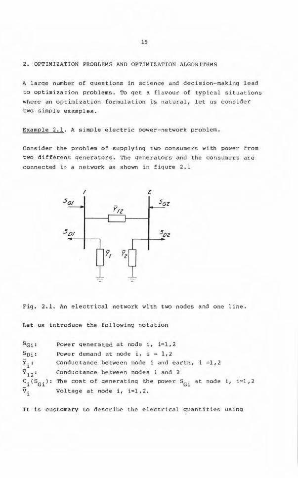
Example 2 . 1. A simple e l ectric power- network problem .

Consider the problem of supplying two consumers with power from

two different qenerators. The qenerators and the consumers are

connected in a network as shown in fiqure 2.1

I z .5G/ 5Gz

Y1z

.501 5oz

r, Yz

Fig. 2.1. An electrical network with two nodes and one line.

Let us introduce the following notation

5 Gi:

Soi :

Y. : l

y 12:

Ci (SGi) :

vi

Power qenerated at node i , i=l,2

Power demand at node i, i = 1,2

Conductance between node i and earth , i =1,2

Conductance between nodes l and 2

The cost of qeneratinq the pcwer SGi at node

Voltage at node i, i=l,2.

i, i =l,2

It is customary to describe the electrical quantities usinq

16

complex numbers ; the power is thus split into a rea l a nd an

reactive part i n t he following way:

Here PGl is the active power and QGl is the r eactive power.

Similar expressions also hold for sG2 ' s 01 and s 02 •

The complex vol t ages and conductances can i n an analogous way

be represented us ing amplitude (V1

) and phase angle (~ 1 ), i.e. - i~ -v

1=V

1• e 1. For v

2 a similar representation can be introduced;

the conductances will be represented analogously , using öi

for t he correspond ing phase a ngles .

The probl em is to satisfy the power demands a t the two nodes ,

and at the same time gener a t e t he powe r as cheaply as poss i b l e .

The l a tter cond ition is expressed as to minimize a criterion

( 2 .1 )

There a r e also a number of physical constraints associated with

this problem . At each nod e there must be a power balance . This

means that the following constraints must be met at node 1 :

( 2. 2)

where * means complex conjugate.

Simi l arly for node 2 we have

(2.3)

Also, the capacities of t he genera tors are limited , wh ich means

t hat constraints of the follow ing t ype

i=l, 2 ( 2. 4)

17

must be included . Similarly, the voltage amplitudes must lie

within certain bounds:

V <V. <V .l- i- u

i=l, 2 ( 2 . 5)

The requirement that the network must be stable corresponds to

a condition on the difference be tween the phase angles :

1t <-

2 ( 2. 6)

Finally, we must introduce a constraint on the heat developed

in the line, assuring that it does not melt down . Such a con­

dition corresponds to

( 2 . 7)

The problem of generating power in the simple network in a sen­

sible way has now been formalized as an optimization problem ,

namely to minimize (2.1) subject to the constraints (2 . 2)-

( 2 . 7) •

0

Example 2 . 2 . Housing maintenance.

(This example is adapted from Luenberger (1979), pp 433). Con­

sider a rental house, and suppose that its state can be charac­

terized by a single quality measure x(k) at time k . A simple

mode l for how this quality measure develops can then be given

as

u2

(k) x(k+l)=cxx(k)+u(k)- --- k=O, •.• , N- 1 x- x(k)

( 2. 8)

here the number a is subject to O<cx<l, describing the decay of

the house with time . The maintenance expenditure during time

period k is u(k) and the value x=x>O corresponds to "perfect

conditions".

18

The rent of the house i s supposed to be proportional to the

guality measure x. The problem we consider, i s that of a land­

lord who wishes to determine a maintenance policy, so as to

maximize a discounted net profit up to a cer t ain time instance

N, when he plans to sell the house. For mally, he wishes to maxi­

mize

N J=13 C x(N)+ N-1 r (px(k)-u(k))l3k

k=O ( 2 . 9)

where p>O , 0<13< l. The guantity C x(N) i s the sales price a t time

N and the guantity p x(k) is the rental income . At the begi nn ing

of t he time period considered, the q uality of t he house is

supposed to be

(2.10)

The optimization problem is then to f ind the seguence u( O), .• . ,

u(N- 1) such that the expression (2.9) is maximized when x(k) ,

k=O, ••. ,N satisfies the const r aints (2.8) and (2.10).

0

The problems considered in exampl e 2.1 and 2 . 2 are quite diffe ­

rent. Still , they coul d both be described by the follow ing for­

mulation

minimize .l(z) (2.lla)

subject to g (z)=O ( 2. ll b)

h( z )2_0 ( 2 . llc)

In example 2.1 we could let the vector z consist of t he para­

meters v1 , ö 1 , v 2 , ö 2 , PGl ' QGl ' PG 2and QG 2 . The functional .l

then corresponds to the functions c1

and c2 in ( 2 . 1) . The

equality cons t raints g correspond to eguations (2.2) and (2.3),

while the inequality co nstraints h in (2. llc ) have their

counterparts in the relations (2.4) - (2 . 7).

19

In example 2.2 the vector z consists of the states x(t),

t=O, ... , as well as the control variables u(t), t=O, .. , N-1. The

function ~ (which often will be ca l led the objective function)

is defined by (2.9) and the equality constraints correspond to

(2 . 8) and (2.10) In this example there are no inequality con­

straints.

In example 2.2 it is possible to arrive at a slightly different

Eormulation by el i minating the states x(k) in (2 . 9) using equa­

tions (2.8) and (2.10). These two equations define the sequence

x(k) , k=O, . .. , N uniquely from the sequence u(k) , k=O, . . . , N- 1 .

Then J in (2.9) will be a Eunction of the control signals u(k),

k=O, •.• , N-1 on l y. In this example (which isa simple case of an

optimal control problem) we thus have the option of considering

both u and x as free variables, subject to a constraint (corres ­

ponding to (2.8)) or to eliminate t he intermedia t e variables x,

and let the vector z in (2 . 11) consist of the control signals

only. In this thesis we shall work with both these variants,

choosing one or the other depending on the situation .

The problem (2 . 11) is the standard Eormulation of the general

nonlinear programming problem. Many algorithms have been pro­

posed for solving this problem, and considerable efforts have

been made to find efficient algorithms for a variety of situa­

tions. What constitutes an efficient algorithm for a particular

case , will be highly dependent on the structure and the com­

plexity of the functions ~' g and h . Important properties are,

for instance, whether these functio ns are linear or non l inear

and if they are differentiable or not. In this thesis we shall

assume throughout that the functions involved are at least twice

continuously dif f erentiable and not necessarily linear. We also

asswne that all second derivatives are Lipschitz continuous.

For unconstrained problems, i.e. problems where (2 . llbc) do not

apply, the most common methods are

Steepes t Descent Method

Newtons ' s Method

Conjugate Oirec t ion Method

Quasi-Newton Methods.

20

(See, for example, Luenberger (1973) and Fletcher (1980)). All

these methods generate a sequence of points, zk, which under

suitable conditions converges to a local minimum of the

criterion (2.lla). This sequence of points is then generated as

(2.12)

where 0 <ak~l is chosen so that a suitable decrease is obtain­

ed in the objective function (2.lla). For the Steepest Descent

Method, the vector dk in (2.12) is t he negat ive gradient, i.e.

For Conjugate Direction Methods, dk is chosen as a certain

linear combination of the gradient ~;(zk) and the previous

direction d k-l' In Newton ' s Method, dk is chosen as the solution

of

where H(zk) is the Hessian of the objective Eunction , i.e.

The calculation of H(zk) and dk may be computationally costly.

Therefore some methods use

where Hk is an approximation of H(zk). Th is approximation is

changed at each step . Such methods are called Quasi-Newton

Methods.

For constrained programming problems {i.e. problems where

(2 . llbc) apply), well known methods are (see Luenberger

(1973) and Fletcher (1981)):

Penal ty and Barrier Methods

The Reduced Gradient Method

Augmented Lagrangian Methods

Feasible Direction Methods

Wilson ' s Method (Wilson, 1963)

21

Quasi-Newton versions of Wilsons Method (Powell (1979), Han

(1975, 1977), and Chamberlain et al. (1979)).

In this thesis we shall concentrate on algor ithms developed from

Wilson' s Method. (Described for instance in Bertsekas (1982)

pp. 252-256.) This method was proposed in 1963 . Since second

order derivatives are required in this algorithm, it is rather

time consuming. Therefore it is not very useful . For sparse

problems (such as those we are to encounter in the later chap­

ters) the computational work may be reasonable. We shall here

give a short motivation and desc ription of Wilson ' s Mehtod.

First, we assume that there are no inequality c onstraints, i.e.

the problem is defined by (2.llab). The Lagrangian of the prob­

lem is t hen given by

T L(Z,A) =~( z)+A g(z). ( 2 .13)

The Kuhn-Tucker necessary conditions (see p. 242 in Luenberger

(1973)) then state that if z* is the solution of (2.11) then

there exists a multiplier A* such t ha t

(2.14a)

g(z*)=O (2.14b)

The relations (2.14) f orm a system of nonlinear equations in the

variables z .and A, Assume that we have a good estimate (zk,Ak)

of the solution to (2.14). This estimate could then be improved

using Newton - Raphson's method (see Dahlquist and Björck (1974),

pp. 249) . Then a new estimate ( zk+l, Ak+l) to the solution of

(2.14) is constructed as follows:

22

Noting that

we can write the equations as

The above equations can however be interpreted as Kuhn- Tucker

necessary conditions for the following optimization problem :

minimize

zk+l

The above equat ion is a q uadrat i c minimization problem with

linear constraints for determining zk+l from zk' ~k. If we had

included inequality constraints (2.llc) we would similarly have

been led to the problem

minimize dk

(2.15a)

(2.15b)

(2.15c)

Here µk are the Lagrangian mul t ipliers to the i nequality con­

straints. With dk determined from (2.15) we then calculate

zk+l using (2 . 12). S ince the described calculations consi-

tute Newton- Raphson steps for solving (2.14) , the sequence zk

will converge quadratically to z* locally , provided ak=l in

(2.12). To assure global convergence, it is sometimes necessary

to let the step length parameter ak be less than unity. Cham-

23

berlain et al. (1979) g ive a useful way to ca l culate ak, which

guarantees both global convergence and fast l ocal conve rgence

under suitable conditions.

In quasi-Newton versions of Wi l son's method, the Hessian of the

Lagrangian in (2.15a), i.e. L22

(zk,Ak,µk), is replaced by an

approximation Hk.

When the non- linear optimization probl em (2 . 11) is generated by

a discrete-time optimal control problem, such as the one in

example 2.2, special methods have been developed to utilize the

particular structure in question . Methods particularly designed

for solving discrete-time optimal control prob l ems can be found

in Bryson and Ho (1969), Dyer and McReynolds (1970), Jacobson

and Mayne (1970), Bellman and Dreyfus (1962) and Ohno ( 1978) .

We shall in th is thesis demonstrate how Wilson's me thod can be

adapted to take the special structure of discrete time - optimal

control problems into account.

For !arge problems, that is when the number of elements in z is

more than, say, 100 , the choice of algorithm for solving the

problem (2.11) is very important indeed. The algorithm must

converge fast and it must be numerically stable. For such prob­

lems it is necessary to take the particular structure of the

problem into account so that suitable decomposi tion t e chniques

can be applied (Lasdon 1970).

A common example of such !arge probl ems is r e a l -li fe power net­

work problems (such as !arge network variants o f example 2. 1 ).

These networks usually have more than 100 nodes, whic h may l ead

to more than 500 unknown parameters . Optimal control problems

similarly lead to !arge optimization prob l ems i f the number o f

time points is large and there are several state variables and

control signa l s .

24

25

3. SOLVING SPARSE QUADRATIC SUBPROBLEMS

3 . 1 Introduction

In chapter 2 we discussed the algori t hm known as Wi l son ' s Met­

hod. In that algorithm one must solve quadratic problems of the type

min z

subject to

T l T b z+7

z B z ,

g +Gz=O ,

h+Hz<O ,

(3 . la)

(3.lb)

( 3 . le)

where z,b,g and h are column vectors of dimensions n , n,m1

and

m2

respectivley, while B,G and H are matrices of appropriate

dime ns ions , with B symmetric . In order to have a uniq ue solution

of (3 . 1) and to ensure that the algorithm will find this solu­

tion, we make the following assumptions about the matrices B, G

and H.

Al: The ma t rix B is positive definite on the null space of G,

i. e. 3 o:> O: T 2

Gz=O => z Bz..'.'._o: J I z I \ ·

A2: The rows of G and H are linearly independent, i.e . the only

solution (~ , µ) of

T T G A+H µ=O

is ~=O and µ=O .

Several rnethods for solving problem (3 . 1) have been given (see

e . g . Gill and Murray (1978)) but few of them can utilize a

sparse structure of the matrices B, G and H.

26

3.2 An algorithm for solving quadratic problems

In this section we will g i ve the basic steps o f an algorithm

proposed by Goldfarb (1975}, which can utilize sparsity in the

matrices B, G and H. The Lagrangian of the problem (3.1) is

T 1 T T T L(Z ,A, µ )=b z+~ z BZ+A (g+Gz)+µ (h+Hz} '

and the Kuhn- Tucker necessary conditions are

T T b+Bz+G A+H µ=0 ,

g+Gz=O ,

h+Hz<O ,

µ~0 and

T µ (h+Hz)=O

(c f pp. 233 in Luenberger (1973)).

( 3. 2)

( 3. 3a)

( 3. 3b)

(3.3c)

(3.3d)

(3.3e)

Lemma 3.1: If the matrices B, G and H satisfy assumptions Al and

A2, then there exists a unique point (Z,A,µ) that satisfies the

conditions (3.3a-e}.

Proof: Exi s t e nce : Because of A2 we know that there exists at

least one point that satisfies the constraints (3.lb) and

(3.lc). Because of Al there is then a solution of (3.1). ror

this solution the theorem on page 233 in Luenberger (1973} gua­

rantees t he existence of multipliers A and µ such that the con­

ditions (3.3) are satisfied.

Uniqueness: Assume that we have two different points, (z1

,A1

,µ1

}

and (z2

,A2

, µ2

) , t hat satisfy the conditions (3.3). If z1

=z2

,

then assumption A2 and the condition (3.3a) imply that A1

=A2

and

µ1

=µ2

so we can assume that z11z

2• from (3.3b} we get

G(z1

-z2

}=0. Hence z1

- z2

is in the null space of G. Similarly

(3.3a) gives

27

Using this together with Al gives

In the last equality we used the conditions (3 . 3e) for z1 and

z2. The above expression contradicts the conditions (3 . 3c) and (3.3d), which proves that we have at most one point that satis­

fies the conditions (3 . 3) .

0

We will now consider ways of so l ving the problem defined by

(3 . la-c). Let the i:th element of h be de noted h. and let the l

i : th row of H be denoted H . • Let J be a given set of distinct l

positive integers j (J is the set of supposed ac tive con-

straint s), s uch that j~m 2 and define hand Has

jiEJ, i= l , ... ,p'

A way of finding the solution of (3 . 3) is given by the following

algorithm.

I . Let z0

be an initial approximation of the solution . Let J

consist of the integers j such that h.+H.z0>o. Let k=O and go to

J J step IL

II . Solve t he system

28

( 3. 4 )

Denote the solution by z ' , A', µ '

II I . I f h+Hz ' <O t hen go t o s t ep I V, o therwise l eta be t he

largest number, such that h.+H . (zk+a(z ' -zk))<O for all integers J J -

j t hat are not yet in J . Add one integer j , for which

hj+Hj(zk+a(z '- zk))=O, t o the index set J. Put zk+l=zk +a(z ' - zk ). Put k=k+l and go back t o step Il.

IV. Put zk+ l=z ' , k=k+l.

If µ!>O for al l j t hen go to V, else de l ete the index j f r om J ]-

for which µ! is mos t negative, and t o back t o step I . J

V. zk is the solution.

This way to choose active constraints is basically the same as

that given i n Gi l l a nd Murray (1978 ) and Powell (1981) . Note

that we do not start to delete any constraints from t he active

set before we have found a point zkthat satisfies h+Hzk~O. After

tha t , every genera t ed point will satisfy this constra i nt a nd the

algorithm will find the solution t o (3.3) af t er a fini t e number

of steps according to section 7 of Gill and Murray (1978) . I f

the a l gorithm fails to f i nd a solution, tha t is if the algor ithm

starts cycling or the matrix in (3 . 4) becomes singular , then the

c o ns t raints are eithe r linearly dependent or t he ma t ri x B i s not

positive definite on the nul l space o f 6. Examples of methods fo r solving the system (3 . 4) can be found in section 5.3 in

Bartels et al. ( 1970) , in Bunch and Kaufman ( 1980) and in Paige

and Sanders (1975).

3.3 How to utilize the sparsity

If we have an initial value z0

, that generates a correct or

almost correct set o f active co nstraints , then we us ua l ly need

29

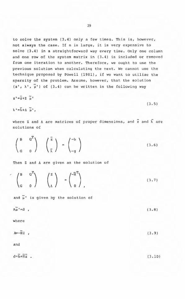
to solve the system (3 . 4) only a few times . This i s , however,

not always the case. If n is large, it is very expensive to

solve (3.4) in a straightforward way every time. Only one column

and one row of the system matrix in (3 . 4) is included or removed

f rom one iteration to another. Therefore, we ought to use the

previous solution when calculating the next. We cannot use the

technique proposed by Powell (1981), if we want to utilize the

sparsity of the problem . Assume, however, that the solution

(z', A1, µ.) of (3.4) can be written in the followi ng way

z ' =z+Z µ. ( 3. 5)

A1 =A+Aµ ' ,

where Z and A are matrices of proper dimensions, and z and A are

solutions of

( 3. 6)

Then Z and A are given as the solution of

{ 3 . 7)

andµ. is given by the solution of

Aµ I =d , { 3 • 8)

where

A=-HZ , ( 3. 9)

and

d=h+ttz (3 . 10)

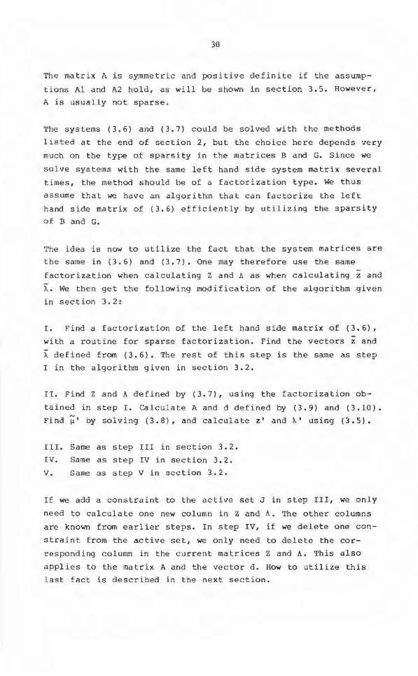
30

The matrix A is symmetric and positive definite if the assump­

tions Al and A2 hold, as will be shown in section 3.5. However,

A is usually not sparse .

The systems (3.6) and (3.7) could be solved with the methods

l isted at the end of section 2, but the choice here depends very

much on the type of sparsity in the matrices B and G. Since we

solve systems with the same left hand side system matrix several

times, the method should be of a factorization type. We thus

assume that we have an algorithm that can factorize the left

hand side matrix o f (3. 6) eff iciently by utilizing the sparsity

of B and G.

The idea is now to utilize the fact that the system matrices are

t he same in (3.6) and (3.7). One may therefore use the same

factorization when calculating Z and Å as when calculating z and

A. We then get the following modification of the algorithm given

in section 3.2:

I. Find a factorization of the left hand side matrix of (3.6),

wi th a routine for sparse f actorization. Find the vectors z and

A defined from (3.6). The rest of t his step is the same as step

I in the algorithm give n in section 3.2.

Il . F ind Z and A defined by (3.7), using the factorization ob­

tained in step I . Calcu l ate A and d defined by (3.9) and (3.10).

Find µ• by solving (3.8), and calcul ate z' and A1 using (3.5).

III. Same as step III in section 3.2.

IV. Same as step I V in section 3.2.

V. Same as step V in sect ion 3.2.

If we add a constraint to the active set J in step III, we only

need to ca l culate one new column in z and A. Th e other columns

are known f rom earlier ste ps. I n step IV, if we delete one con­

straint from the active set , we only need to delete the cor­

r espond ing column in the curre nt matrices z and A. This also

appl ies to t he matrix A and the vector a. How to uti lize this

l ast fac t i s described in the next section.

31

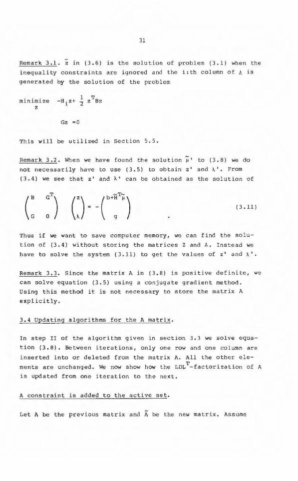
Remark 3.1. z in (3.6) is the solution o f problem (3 . 1) wh en the

inequality constraints are ignored and the i : th column of A is

generated by the solution of the problem

minimize z

l T -H i z+ "'2 z Bz

Gz =O

This will be utilized in Section 5.5.

Remark 3.2. When we have found the solution);• to (3.8) we do

not necessarily have to use (3.5) to obtain z ' and A' · From

(3.4) we see that z' and A' can be obtained as the solution of

(3 . 11 )

Thus if we want to save computer memory, we can find the solu­

tion of (3.4) without storing the matrices Z and A. Instead we

have to solve the system (3 . 11) to get the values of z ' and A1•

Remark 3 . 3. Since the matrix A in (3.8) is positive defi nite, we

can solve equation (3.5) using a conjugate gradient method.

Using this method it is not necessary to store the matrix A

explicitly.

3.4 Updating algorithms for the A matrix .

In step II of the algorithm given in section 3 . 3 we solve equa­

tion (3 . 8). Between iterations, on l y one row and one column are

inserted into or deleted from the matrix A. All the other ele­

ments are unchanged. We now show how the LDLT-factorization of A

is updated from one iteration to the next.

A constraint is added to the active set.

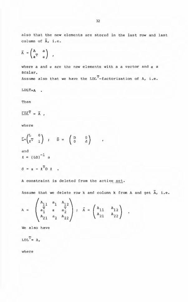
Let A be the previous matrix and A be the new ma trix . Assume

32

also that the new elements are stored in the last row and las t

column of A, i.e.

- (A A = aT

where a and o; are the new elements wi th a a vector and o: a

scalar.

Assume also that we have the LDL T-factorization of A, i .e.

LDLT=A

Then

LÖLT A

where

E= GT ~ ) D ( D ~ ) 0

and

.R. = (LO) - l a

d o:-.R.TD.R.

A constraint is deleted from the ac tive set.

-Assume that we delete row k and column k from A and get A, i.e.

A

We also have

T LDL = A,

where

A

33

0

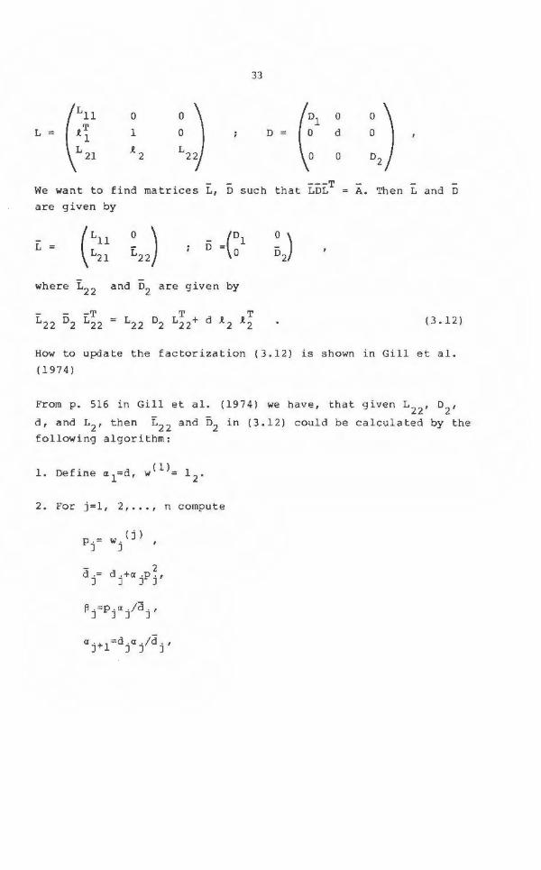
- ---T - - -We want to find matrices L, D such that LDL = A. Th e n L and D

are given by

L ( Lll L21 ~,,) - (Dl D =

0 ~J where L22 and 02 are given by

L22 -T T 1T (3 .12) 02 L22 = L22 02 L22+ d 12 2

How to update t he factorization (3.12) is shown in Gill e t al.

(1974)

From p. 516 in Gill et al. (1974) we have, that g ive n L22

, o2

,

d, and L2 , then 122 and ö2 in (3.12) could be calculated by the

followi ng algorithm:

2. For j=l, 2, ... , n compute

P .= W • ( j) I

J J

a ·+i=d .a ./d., J J J J

L . +~. w(j+l} rJ J r

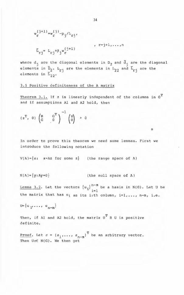
34

, r = j+l , ... ,n

where d. are the diagonal eleme n ts in o2 and ä. are the diagonal J - J

e l emen ts in o2 . Lrj are the elements in L22 and Lrj are the

e l ements in E22 •

3.5 Positive definiteness of t he A matrix

Theorem 3.1. If z i s linearly i ndependent of t he columns in GT

and if assumptions Al and A2 hold, then

0

In order to prove this theorem we need some lemmas. First we

introduce the following notation

V(A}={x: x=Az for some z} (the range space of A)

N(Al={y: Ay=O} (the null space o f A)

{u.} n-m Lemma 3 .2. Let the vectors be abasis in N(G}. Let u be 1 i=l

the matrix t ha t has ui as its i:th column, i=l, .•• , n-m, i.e.

U= { u l' ... ' u n-m}

Then, if Al and A2 ho ld, the matrix UT B U is positive

definite.

T Proof. Leta = (a1 , ... , crn-m} be an arbitrary vector.

Then UcrE N(G}. We then get

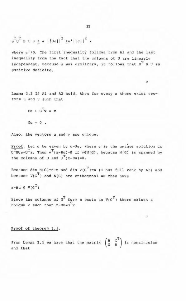
35

T T 2 2 crU BUcr~a l! Ucrjl ~a'l\crll '

where a ' >O. The first inequality follows from Al and the last

inequality from the fact that the columns of U are linearly

independent. Because a was arbitrary, it follows that UT B U is

posit ive definite.

Cl

Lemma 3 . 3 If Al and A2 hold, then for every z there exist vec­

tors u and v such that

Gu 0 .

Also, the vectors u and v are unique.

. Proof. Let u be qiven by u=Ua, where a is the unique solution to -T-- T T U BUa=U z. Then v (z-Bu)=O if vEN(G), because N(G) is spanned by

the columns of u and UT(z-Bu)=O .

Because dim N(G)=n-m and dim V(GT)=m (G has full rank by A2) and

because V(GT) and N(G) are orthoqonal we then have

Since the columns of GT form a basis in V(GT) there exists a . h T un1que v such t at z - Bu=G v.

Proof of theorem 3.1 .

From Lemma 3 . 3 we h ave that the ma trix

and that

Cl

(~ GOT) is nonsinqular

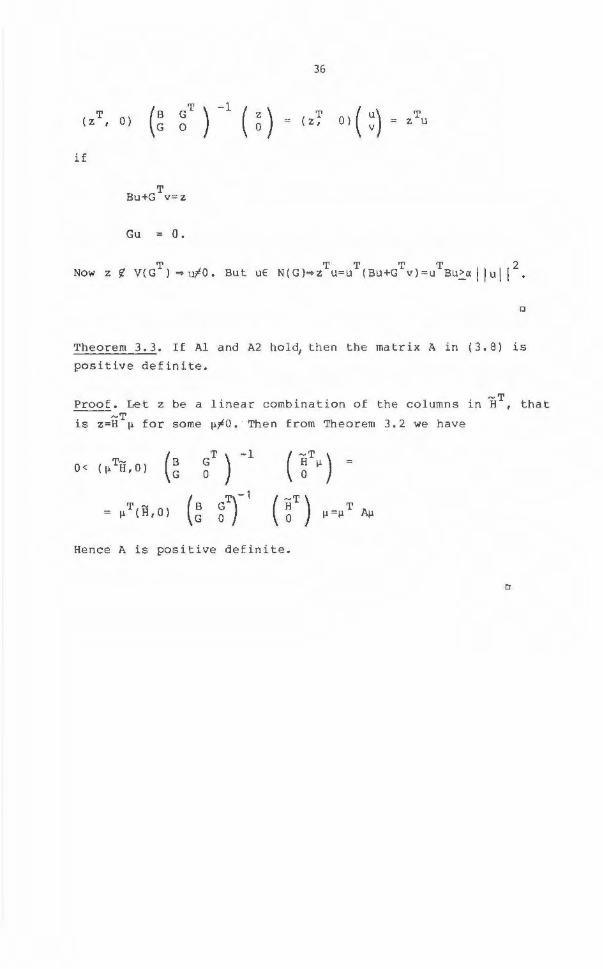
T ( z , 0} ( ~ if

T Bu+G v= z

Gu 0 .

36

T ( z, T z u

T T T T T 2 Now z !(' V(G ),,.\lfO . But uE N(G)""Z u=u (Bu +G v)=u Bu~o:/ l u ll ,

0

Theore m 3.3 . If Al and A2 ho l~ then the matrix A in ( 3 . 8 ) is

pos i tive de finite .

Proof . Let z be a linear comb ination o f the columns in HT, t hat --~T

is z=H µfor same µ~O . Then from Theorem 3 . 2 we have

O< T~ ( µ H, 0} ( ~ ~T ) - 1 ( ~Tµ)

T ~ (~ ff1 ( ~T ) T Aµ µ (H,0} µ =µ

He nce A is positive definite.

0

37

4. NONLINEAR OPTI MAL CONTROL PROBLEMS

4.1 Problem definition

In this chapter we will consider optimal control of discrete

time dynamical systems, described in s t ate space form . At time

instant t, the system is desc ribed by a state vector x (t) of

dimens ion n and a control vector u(t), of d imens ion n . Over X U

t he time horizon t=O , l , .. . ,N the system is assumed to be

d escribed by the difference equation

x(t+l)=f(x(t ),u(t ) ,t ), t=O, . .. ,N-1 . ( 4 .1 )

Here f is a vector function of di mens ion nx. The initial state

o f t he system is given by

( 4 . 2)

we want to choose the sequence of input vectors u(t), t=O, ... ,

N- 1 so that the s ystem behaves i n some desired man ner. Suppose

that we can measure how well the system satisfies our objec t ives

by the performance inde x

N-1 J(u)=1(x(N),N)+ E 1(x(t) ,u( t) , t)

t=O ( 4 . 3)

whe re the f unc tions 1 are sca l ars. Fr om equations (4 . 1) and

(4 . 2) we see that the sequence.of sta t e vectors, x(t), i s uni­

quely de t ermined , once we have chosen the control variable s

u(t) . Hence the performance index ( 4. 3) is a function of t he

centrals u(t) . Th i s fac t is stressed by the argument u in J(u) .

For safe operation of the system, it might be requ ired that its

states rema i n within certain limits , that may depend on t i me .

Also , the input variable may be restricted in same way. To in­

corporate t h is situation in the formal description, we add th e

following cons traints

38

hi(x( t.) , u(t.) )<0 ,i=l , ••. ,p, 1 1 -

( 4. 4)

to the system description. Here ti are integers satisfy ing

O..::_ti~ N and hi are scalar functions. The number of con­straints at a given time instant may vary from instant to

instant, that is , the t. :s in (4 . 4) need not be different. In 1

(4.4) we may also easily incorporate terminal constraints ,

involving the state x(N) only .

The functions f, 1 and hi in (4.1) , (4.2) and (4.4) are all

supposed to be twice continuously differen t iable with respect to

x and u. Furthermore , the second order der i vatives are supposed to be Lipschitz con t inuous in x and u. 'lhe optimal control prob­

lem is now t o select the control variables u(t), t=O ,l ••• , N-1 so

t hat the performance index (4.3) is minimized, whi l e t he con­

straints (4.4) are satisfied. We r ecognize the housing main­

t e nance problem , example 2. 2 , as a simple example of t his

general problem formulation.

4.2 Optimal control methods

Many computational me thods have been designed to solve the opti­

mal control problem defined in the previous section . Mast of

these methods use dynamic programming techniques. In dynamic

programming , the optimal value function v0 (x(t) ,t) is defined as

0 V (x(N) ,N)=.t(x(N) , N) (4.Sa)

v0 (X ( t ) , t ) =min { .t ( X ( t) 'u ( t) 't ) + v0

( f ( X ( t) ' u ( t ) 't ) , t + 1 ) } • ( 4 . 5 b) u( t)

The basic idea behind the methods proposed in Mayne (1966) and

Dyer and McReynolds (1970) is to use (4.Sb) to find the incre­

ment u(t) that minimizes the second order Taylor expansion of

the expression within curly brackets in (4.Sb). In order to

accomplish that , the first and second order derivatives of v0

with respect to x are assumed to exist.

39

The perhaps best known method for solving optimal control prob­

lems is the d i fferential dynamic programming (DDP-method) pro­

posed by Jacobson and Mayne (1970). Th is method employs a global

minimization with respect to u(t), after which the right hand

side of (4. 5b) is expanded to second order around this control.

Another, very similar, algorithm is described in Mitter (1966),

and McReynolds and Bryson (1965). This latter method requires

the solution of an extra set of vector difference equations. The

method is very c l osely related to the one that we will derive in

section 4.3.1.

None of these methods is very good at handling constraints of

the type (4.4). However, if these constraints are explicit func­

tions of u( t), then they can be handled by a method proposed by

Ohno (1978). This method is based on the fact that the Kuhn­

Tucker conditions must be satisfied (pointwise in time) for t he

minimizing values in (4.5b), subject to the constraints (4 . 4) . A

comprehensive survey of the methods for optimal control is given

by Polak (1 973), and the reader is referred to this reference

for further details.

4.3 Newton ' s method for optimal control problems

As we remarked earlier, the performance index (4.3) isa func­

tion of the control variables u(t), since the sequence of state

vectors is uniquely determined as functions of u(t) . The same is

of course true also for the constraints (4 . 4) . This means that

the optimal control program (4.1)-(4.4) is a problem of the type

(2.11), where the inputs u(t),t=O, ... ,N-1 are the unknown para­

meters. When we applied Wilson' s ( 1963) method to the problem

(2.11), we ended up with the quadratic subproblem (2.15). Here,

we shall derive the corresponding quadratic subproblem, when

Wilson ' s method is applied to the optimal control problem. The

case with no constraints is handled in section 4 . 3.1. Section

4 . 3.2 deals with a case when there is only one constraint of the

type (4.4), whi l e t he general case is deferred to section

4.3.3.

40

i~~~!-~~~!~~~!~~-~~-~~~-9~~~~~~!~-~~~e~~~!~~~-!~~-~~~~-9~-~Q-cons t r a in t s .

Le t the vector z(t) contain all the control variables from time

t up to time N-1 :

T T T T z ( t) = ( u ( N- 1) , u ( N- 2) , .•• , u ( t) ) ( 4. 6)

Note t hat z(t) satisfies the recursion

T T T z(t) =(z (t+l),u (t)) ( 4. 7)

Let us also introduce the function V( x (t) ,z(t) ,t ) which is t h e

cost from time t up to time N when starting in state x( t) and

using the control z( t ) . These f unctions can formally be written

as

V( x(t ) , z( t) ,t )=.l(x(t) ,u (t) ,t)+V( f(x(t) , u( t) ,t) , z(t+l) ,t+l)

( 4. 8)

Notice the diff e r ence betwee n v0 in (4.5) and V in (4.8 ). V is a

function of z(t) whereas v0 is the infimum of this function with

respect to z(t) for t he same x(t). Clearly, mi n imi zing the per­

formance i ndex (4.3) , subject to (4.1)-(4 . 2) is the same problem

as t hat of minimizing V(0

, z(0) , 0) with r espect to z(O). Conse ­

quently , by t he introduction of the functions V in (4 . 8) we have

rewritten the optimal control p roblem (4.1)-(4. 3) as an uncons t­

rained minimization problem for the fu nctions V(x0

,z (0) , 0) in

the variable z( O). Let us s o lve this problem using Wi l s on' s

(1963 ) method . Wilson ' s method reduces to Newton ' s me t hod, whe n

applied toan unconstrained problem (see Luenberger (1973) , p .

1 55) . The method is thus as follows : Le t Zk( O) be an approxi­

mation to the solution. Let W(t.z(O) , 0) be the second order

Taylo r expansion of V(O) around this point , i.e.

41

3 V(x 0 ,zk(O)+llz(O) ,o, )=W(llz(O) ,O)+O( \llz(OJ I )

or

A better approximation to the solution is now found by mini ­

mizing (4 . 9) with respect to llz(O) and adding the minimizing

argument to zk(O), i.e.

where

To improve the convergence properties, eq . ( 4 . 10) is usually

modifi ed to

where ak is a scalar in the interval (0,1]. In chapter 8, we

shall discuss how this scalar should be chosen . Por convenience,

we have suppressed th e arguments x0

and zk (0) in the above ex­

press ions . We shall do so al so in the sequel , when there is no

risk of confusion .

The expression (4.10) contains t he first and second order deri­

vatives of V(O) with respect to z (O) . The following lemma

guarantees that these derivativeB exist.

Lemma 4 . 1 . Suppose that that the Eunctions E and~ in (4.1) and

(4. 3) are twice continuously differentiable with respect to x

and u, and that the second derivatives are Lipschitz continuous

in x and u . Then t he functions V(x(t) ,z(t ),t) in (4 . 8) are tw i<:e

continuously differentiable with respect to x and z, and the

second order derivatives are Lipschitz continuous in x and z .

42

Proof. The lemma follows trivially by induction on (4.8) and

from Theorem 9.12 in Rudin (1964).

0

From the lemma it also f o llows that the following derivatives

exist :

V (N)=i (x(N)) X X

(4.12a)

V (N)=i (x(N)) XX XX

(4.l2b)

which fol l ows from (4.8a). From ( 4. 8b) and (4.7) we further get

(4.12c)

V (t)=(V (t+ l ), 1 (t) +V ( t+l) f ( t )) Z Z U X U

(4. 1 2d)

T V (t)=~ (t)+V (t+l)f (t)+f (t)V (t+l) f (t)

XX XX X XX X XX X (4.12e)

V (t)=(fT( t )V (t+l ),1 ( t )+V (t+l)f (t)+fT(t)V (t+l )f (t)) XZ X XZ XU X XU X XX U

(

V ( t+l ) V ( t)= zz

zz f ~(t)Vx2 (t+l )

(4.12f)

V (t+l )f (t} ) zx u

1 (t}+V (t+l)f (t)+fT(t)V (t+l)f (t) UU X UU U XX U

( 4. l 2g)

These derivates are all evaluated at the point (x( t ) , z(t)) ,

where x(t) satisfies (4.l) and (4.2) for all t , and u(t) is

given by z ( 0 ) .

Let W(t)=W ( öx(t),öz(t} , t) be the second order Taylor e xpansion

of the f unc t ion V(t) around the point (x(t) , z(t)), i.e.

43

V ( X ( t ) +ti X ( t) I z ( t) +ti z ( t) It) =W ( t) +O ( I~;~ ~ ~ 13 ) ( 4 . 13)

or

(4.14)

If we now substitute V(t), Vx(t), Vz(t), Vxx(t), Vxz(t), V22

(t)

and z(t) in (4.14) using the expressions (4.Sb), (4.12c) - (4 . 12g)

and (4.7) we get

+ ~ (6XT(t)(.t (t)+V (t+l)f (t)+fT(t)V (t+l)fx(t))t.x(t) + L. XX X XX X XX

+26xT(t)(.t (t)+V (t+l)f (t)+fT(t)Vxx(t+l)fu(t))t.u(t)+ XU X XU X

+t.zT(t+l)V (t+l)6z(t+l)+26uT(t) fT(t)V (t+l)t.z(t+l)+ zz u xz

(4 . 15)

By rearranging the terms in (4. 1 5) and introducing the aux iliary

variable D(t+l) as

D(t+l) =fx(t)6x(t)+fu(t)6u(t), ( 4 .1 6)

we can write (4 . 15) as

W(t)=V(t+l )+V (t+l)D(t+l)+V ( t+l )6Z(t+l)+ X Z

44

+özT(t+l)V (t+l)öz(t+l)) +l(t)+l (t)öx(t)+ ZZ X

+26xT(t)(l (t)+V (t+l)f ( t))öu(t)+ XU X XU

+öuT(t)(l (t)+V (t+l)f (t))öu(t)) UU X U U

Here we can identifiy the first part (cf (4.14)) as

W(D(t+l), öz(t+l) , t+l) .

Hence

W(öx(t) , öz(t) ,t)=W(D(t+l) , öz( t+l),t+l )+l(t)+l (t)öx(t)+ X

+l (t)öu(t)+ 12

(öxT(t)(l (t)+V (t+l) f (t))öx(t)+ U XX X XX

(4.17)

( 4 .18)

where D(t+l) is given by (4.16). Notice that this auxiliary

variabl e satisfies the dynamics of (4.1) , when linearized around

(x(t) , u(t) ). Therefore we shall hencefort h use t he natural nota­

tion öx(t+l) instead of D(t+l). (See eq. (4 .20b) below.) Let us

also introduce t he notation

(4.19a)

Q (t)=l (t)+V (t+l )f (t) XX XX X XX

(4.19b)

Q (t) =l (t)+V (t+l) f (t) XU XU X XU

(4. 19c)

45

Q (t)=! (t)+V (t+l ) f (t), UU UU X UU

(4 . 19d)

where Vx(t) is defined by (4 . 12a) and (4 . 12c) .

El iminating W(t) for t =O, .. ,N-1 in (4.9) using (4.18) we obtain

N-1 + E

t=O {i (t)llx(t)+! (t) llu(t)+; (llxT(t)Q (t)llx(t)+

X U It. XX

+2llxT(t)Q (t)llu(t)+lluT(t)Q (t)llu(t)J ) . xu uu

The aux iliary va r iables llx(t) ,t=O, ... ,N must satisfy

ll x(O)=O

With

T T T llz(O) =(llu (N - 1) , . . . , llu (0)) .

( 4 . 20a )

(4 . 20b)

(4 . 20c)

We notice that the expression ( 4 . 20) is the same as ( 4 . 9) . Con ­

seguently , mi nimization of (4 . 20a) under th e constraints

(4.20 bc) will give the same sequence llu(t) ,t=O , .. ,N-1 as

( 4 . 10) .

In the li t erature , the problem (4.20) is usually called t he

linear-quadratic control problem , since the dynam i cs is linear

in ll x( t) and llu ( t), and the performance index is quadratic in

these variables . The standard linear-quadra tic control pr0blem ,

however , con t ains no linear terms in the pe rformance index

(4.20a) . For further details see Kwakernaak and Sivan (1972), p .

490, Dyer and Mc Reynolds (1970), p . 42 or Bryson and Ho (1969)

p . 46 .

We shall discuss two different approaches to solving (4. 20) . In

46

chapter 5 , we shall solve the eguations t ha t correspond to the

Kuhn -Tucker necessary condit i ons for (4.20). In this section, we

shall solve the problem by introducing a seguence of sub­

prob l ems . These subproblems are :

minimize t.z ( t)

1 T J(t,x (t), t,z{ t ))=lx (N)t,x{N)+ 7 t,x (N)Qxx(N)t,x{N)+

N-1 + E {1 (s) t.x(s) +l (s)t,u(s)+ 1 (6xT(s)Q (s)t.x(s) + s=t X U °2 XX

T T } +2t. x (s)Qxu{s)t.u{s)+t,u {s)Quu{s)6u{s)) .

Subject to

6 X ( s+ 1 ) = f X ( s) t, X ( s) + f u ( s) t, u ( s) , s= t , .• . , N-1

( 4. 2l a)

( 4. 21 b)

Let J*(t,x(t) ,t) be the value of the objective function in

(4 . 21a) corresponding to the optimal control sequence

t.u(s) ,s=t, •• ,N-1. We s hall now proceeed to show that this

function is guadratic in t.x( t) , i.e.

J*(t,x ( t) ,t) =a (t)+W ( t )t,x(t)+ ! t,xT(t)W (t)t,x{t) X ~ XX {4.22)

for some a(t) ,Wx(t) and Wxx(t). Cl early, t his holds for t=N, since

J*( t,x{N) ,N) =lx(N)•t,x (N)+ l 6XT{N)Q (N) t,x (N) 7 XX

( 4. 23)

Hence

a(N) =O (4.24a)

W (N )=1 (N) X X

{4.24b)

{4.24c)

Suppose now that (4.22) holds for t =N , .• . ,p+l. Then

47

1 T J*(6x(p) , p)=min {1 (p)6x(p)+1 (p)6u(p)+ ~ (6X (p)Qxx(p)6x(p)+

6 u ( p) X U "'

+26xT(p)Q (p ) 6u(p)+6uT(p)Q (p)6u(p) )+ xu uu

+J*(f (p)6x(p) +f (p)6u(p) , p+l) } (4.25) X U

The 6u(p) that minimizes the right hand side of (4 . 25) is given

by

( 4 . 26)

Substi t uting 6u(t) in (4.25) by the expr ession (4.26) we find

that J*(6x(p) ,p) is also quadratic in 6x(p) and that the co­

efficients are given by

1 a(p)=a(p+l)- 2 (1u(p)+Wx(p+l)fu(p))(Quu(p)+

T -1 T +fu(p)Wxx(p+l)fu(p)) • (1u(p)+Wx(p+l)fu(p)) ( 4. 27a)

W (p)=1 (p)+W (p+l)f (p)-(1 (p)+W (p+l )f (p))• X X X X U X U

(4 . 27b)

(4.27c)

By induction, we have consequently proved that (4 . 22) holds and

48

tha t t he coeff icients in these functions are given by (4. 24) and

(4.27). Notice that (4 .27 c) is the discrete-time matrix Riccati

equa tion.

For convenience we introduce the fo llowing notation:

ÖU( t)=-( Q ( t)+fT(t)W (t+l)f (t) Jl( ~ (t)+W (t+l)f (t))T (4.28) UU U XX U U X U

and

( 4. 29)

With this notation, equation (4 . 26) can be rewritten as

6u (t)=öu(t) - /:ltÄX (t). ( 4 . 30)

The above shows that the problem (4. 20) can be solved iterative­

l y by sol ving t h e subproblems (4. 21). The value of the perfor­

mance index at the solution to these subproblems is given by

(4.22) where t he coefficients are give n by (4.24) and (4 . 27).

Finally, the solution to (4.20 ) is given by (4.30) where tix(t)

is given by (4.20bc).

We are now ready to summarize the minimization of the performan­

ce index (4.3) using Newton ' s method, when no constraints (4.4)

are present .

Algorithm 4.1.

I . Let an initial control sequence z0

(0) be given (where z(O)

is defined in (4 . 6)) , and pu t k=O.

II. Calculate and store the states x(t), t =O, ... ,N for zk(O)

accoi:-ding to (4 . 1) and (4. 2) . Calculate and store the

va lue o f the objective function (4.3).

49

III. For t =N, ... ,O solve eguations (4 . 12c) and (4.27) with the

initial values (4.12a) and (4.24) respectively . During

these calculations compute and store ou (t} and ~ t given

by (4.28) and (4.29) .

IV. (

N-1 If E

t=O number,

)

1/2 cSu( t) j 2 < er where e is a small positive

go to step VII.

v. Let the elements t. u(t) in t.zk(O) be given by (4 . 30) , in

which t.x(t) satisfies (4.20b) and (4 . 20c) .

VI. Put zk+l{O)=zk(O)+akt.zk(O), where ak is chosen in the

interval (0,1 ) such that a sufficient reduction is

obtained in the performance index (4.3) whe n using the

control zk+l(O) instead of zk(O). Let k=k+l and go back to

step I I.

VII. Stop. zk(O) is close to a local minimum point .

Remark 4 . 1 . In the above algorithm we assumed that the matrices

Q (t)+fT(t)W {t+l)f (t), t=O, .. • ,N-1 are positive definite for UU U X X U

all k. In chapter 6 we shall discuss how to modify the algorithm

if this is not the case .

Remark 4 . 2. It i s not trivial to chose ak in step VI.

Different choices will be discussed in chapte r 7 .

a

a

We are now able to campare the method presented here with some

of those mentioned in section 4.2. Let us start with some com­

ments on the results of Mitter (1966) {cont i nuous time) and

McReynolds (1 966) (as described in Bryson and Ho (1969)). Both

so

these authors have derived the same results as those given here,

but they propose that the control shoul d be given by

(4.31)

instead of (4.30). In (4.31) the state xk+l(t) is the result of

the control uk(t)+6u(t). (For simplicity we assume that ak=l.)

This modification saves computer time, since it is no longer

necessary to solve (4 . 20bc). However, with (4.31) we no longer

take a Newton step towards the solution (cf equations (4.9) and

( 4 . 10)).

The methods proposed by Mayne ( 1966) and Dyer and McReynolds

(1970) differ from the method discussed here in the following

way. First they use (4.31) instead of (4.30). Second , they use

the vectors W (t) given by (4.24b) and (4.27b) instead of the X

vectors Vx(t) given by (4.llad), when calculating the matrices

Q (t), Q (t) and Q (t) in (4.19). With this change it is not XX XU UU

necessary to solve the difference equation (4.l l d), and hence

less computer work is required. But again, the method is no

longer the true Newton method (as claimed in Dyer and McReynolds

(1970) , p. 69). Close to the solution z*(O) these differences

are marginal since

(4.32)

and

(4.33)

as zk(O) + z*(O).

Clearly when the dynamics (4 . 1) is linear in the variables x and

u, all the described algor ithms are identical.

51

constraint.

Now assume that we have one constraint of the type (4.4) and

that this constraint is active at time t=s :

h(x(s) ,u(s) )20, (4.34)

where h is a scalar function. As remarked earlier we can view

x(s) as a function of x0

and z(O) , where z(O) is de f ined by

(4.6). To find these functions and derivatives we proceed as

with V(t) in (4.8). Consequently, introduce the functions

H(x(t) ,z(t) ,t) through

H (X ( t) , z ( t) , t) =O, t>s (4.35a)

H(x(s) ,z(s) ,s)=h(x(s) ,u(s)) (4 . 35b)

H (X ( t) , Z ( t) , t) =H ( f (X ( t) , U ( t) , t) , Z ( t + l) , t + l) , t < S. (4.35c)

As in Lemma 4.1 it follows that these functions are twice diffe­

rentiable and that they are given, for t=s, by

(4.36a)

H (s)=(O,h (s)) z u

(4 . 36b)

H (s)=h (s) XX XX

(4.36c)

(4 . 36d)

(4 . 36e)

and for t <s by

( 4. 36f)

52

H (t)=(H (t+l) ,H (t+l)f (t)) Z Z X U

(4.36g)

(4 .36 h)

H (t)=(fT(t)H (t+l),H (t+l)f (t)+fT(t)H (t+l)f (t)) (4.36i) XZ X XZ X XU X XX U

(

H (t+l) H (t)= zz

ZZ fT(t)H (t+l) u xz

(4.36j)

Our problem now is to fina the value of z(O) that minimizes

V(x 0 ,z(O) ,O) subject to the constraint

where V(O) is given by (4.8) and H(O) by (4 .35) . (Recall our

convention of supressing the arguments xo and z(O).) This isa

problem of the type (2.11) . For our problem, Wilson's method

(corresponding to equations (2.15)) takes the form

(4.37a)

(4.37b)

where the matrix Vzz(O) is given by

(4.38)

and µ is the Lagrange multiplier corresponding to the constraint

(4.34). We shall now reformulate the problem (4.37) in the same

way as we did in the previous s ubsection where (4.9) was re­

written as (4.20). We start by introducing the func tions W(t)

which are analagous to W(t) in (4.14). They are defined by

53

( 4. 39)

whei:-e

~ {t)=V (t) + µH (t) XX XX XX

(4.40a)

(4.40b)

( 4 . 40c)

and V(t ) is given by (4.8). The mati:-ices on the i:-ight hand side

of (4 .40) ai:-e eithei:- given by (4 . 12) oi:- by (4.36) . Foi:- t>s the

functions W(t) and W(t) ai:-e identical . Foi:- t<s we shal l now i:-e­

wi:-ite W(t) in the same way as W{t) was i:-ewi:-itten in (4.18). Fi:-om

( 4.40) and (4 . 39) we have

U s i ng { 4 • 7 ) , { 4 • 8 ) , ( 4 • 12 ) and { 4 • 3 6 ) we ge t

71 {6xT(t)(l (t)+V (t+l)f (t)+fT(t)V (t+l)f (t)+

XX X XX X XX X

+µH (t+l)f (t)+µfT(t)H (t+l)f (t)) 6x(t)+ X XX X XX X

+26xT( t )fT(t)(V (t+l)+µH (t+l ))6z(t+l)+26XT(t)(l (t)+ X XZ XZ XU

+V ( t+l) f ( t )+fT(t)V (t+l)f (t)+ X UU X XX U

54

+özT(t+l)(V (t+l)+µH (t+l))6z(t+l)+26zT(t+l)(V (t+l)+ zz zz xz

+µH (t+l))f (t)6u(t)+6UT(t)(..t (t)+ zx u uu

+V (t+l) f (t)+fT(t)V (t+l)f (t) + X UU U XX U

Again we introduce the auxiliary variable D(t+l) as (4.16) and

then let öx(t+l)=D(t+l). The above equat ion could then be

written

W(t)=..t(t)+W(t+l)H (t)öx(t)H (t)öu(t)+ X U

+ ! 6XT(t)(..t (t)+(V (t+l)+µH (t+l))f (t))öx(t)+ .:. XX X X XX

+26xT(t)(..t (t)+(V (t+l)+µH (t+l))f (t))öu(t)+ XU X X XU

(4.41)

Performing the same calculations for t=s gives

W(s)=..t(s)+W(s+l)+..tx(s)6x(s)+..tu(s)6u(s)+

(4.42)

From (4 . l2c) and (4.36f) we have

55

= .l ( t ) + ( V ( t + l ) + µH ( t +l ) ) f ( t ) X X X X

for t<s and for t=s we have

Now introduce the row vec tors Vx(t) and the matrices

axx(t) ,axu(t) and ~uu(t) as

and

tls

( 4 . 43)

( 4. 44)

( 4 . 45a)

(4.45b)

(4.45c)

( 4. 46a)

(4 .46b)

(4. 46c)

(4. 46d)

(4.46e)

(4.46f)

(4.46g)

From equations (4.41)-(4.46) we see that W(O) can be written

56

W(O)=V(0)+1x(N)6x(N)+ 1 6xT(N)Q (N)6x(N)+ 7 XX

N- 1 + E (1 (t)öx(t)+1 (t)6u(t)+ ~ (6xT(t)Q (t)öx(t)+

t=O X U L. XX

( 4. 4 7)

where the auxiliary variabl e 6x(t) satisfies (4.20bc).

Hence solving the problem (4.37) will give the same 6U(t) as the

so l ution to:

minimize 1x(N)6x(N)+ ~xT(N)Qxx(N)6x(N)+ öu(t)

N- 1 + E {1 (t)6x(t)+1 (t)öu(t)+; (öxT(t)Q (t)öx(t)+

t=Q X U L. XX

subject to 6x(t+l)=fx(t)6x(t)+fu(t)6u(t)

öx ( 0) =0

( 4 . 48a)

(4.48b)

( 4. 48c)

(4.48d)

!~~~~-Q~E~~~~i2~_2f_!b~-9~~~E~!l~-§~~eE2~!~~~-~b~-~~~~-~!-severa1 constraints. -------------------We shall now generalize the results of t he previous subsection

to the case of several cons traints of the type (4 . 4). To ao this we need some instruments to indicate which constraints that are

associated with a particular time instant. Therefore we intro­

duce the sets I(t) as

I(t)={ i : t.=t}. l

( 4. 4 9)

57

This definition of I(t) is illustrated by the following

example .

Example 4.1 . Let the constraints be given by

l h (x(2),u(2)).:_0

2 h (x(2) , u(2)).:_0

and let N=3. Then I(O)=I(l)=!1, !(2)={1,2} and I(3)o:{3} .

we also introduce the functions

i y(t)=y(x(t) , u(t),µ,t)= E µ.h (x(t.),u(t.)). iEI(t) 1 1 1

where µ now isa vector with the compon e nts µ .. l

0

( 4. 50)

In section 4 . 3 . 2 we found that the objective function in (4 . 20a)

was cha nged to (4.48a) in case of one constraint. This con­

straint changed the calculation of Vx(t) in (4.12c) to the

calculation of Vx(t) in (4.45). Also the calculation of Qxx(t),

Q (t) and Q (t) changed from (4.19) to (4 . 46) . If we examine xu uu these changes we see that they are linear. Hence adding more

constraints will only result in linear changes in V(t),Q (t), XX

Qxu(t) and Quu(t). Hence in case of several constraints we then

let V ( t ) be given by X

V (N)=t (N)+y (N) X X X

( 4. 5la)

v ( t l = t ( t l + v < t + l l t < t l +y ( t l X X X X X

( 4 . 5lb)

58

( 4. 52a)

o (t)=-t (t)+v (t+l)f (t)+y (t) XX XX X XX XX

(4. 52b)

( 4. 52c)

o (t)=-t (t>+v (t+llf (t>+r (t) UU UU X UU UU

(4. 52d)

If we use Wilson's method to fina the z(O) that minimizes the

performance index (4.3) while satisfying t he constraints (4.4)

the increments in zk(O) are given by 6z(0) in which 6u(t) is

given by the solution to

1 T ~ minimize ,lx(N)6x(N)+ 7 6x (N)Qxx(N)6x(N)+

6u(t)

N-1 + E {-t {t)6x(t)+-l (t)6u(t)+ 1 (6xT(t)Qxx(t)6x(t)+

t =O X u ""2

+2llxT(t)Q (t)llu(t)HuT(t)Q (t)6u(t)) } xu uu (4.53a)

( 4 . 53b)

6x(0)=0 (4.53c)

(4 .53d)

where Q (t), Q (t) and Q (t) are given by (4.51) and (4.52). XX XU UU

In chapter 5 we shall dicuss one method fo r f inding the solution

to (4.53) as well as the values of the corresponding multipliers

µi · If this method to calculate the increments in z( 0), con­

verges , then the convergence will be of second order. This

follow s since Newton's method is of second order.

59

4.4 Summary

The long and technical calculations in this chapter can be

summarized in the fo llowing theorem :

Theorem 4.1. Suppose that the solution to (4 .5 3) exists and is

unique. Let this solution be denoted by öu (t) . Then öu(t) is the

update that is assigned to the control variable u(t) when

Wilson ' s method is applied to the optimal control problem (4.1) ­

( 4. 4) •

0

The existence of a unique solution to (4 . 53) will be investi­

gated in t he next chapter.

60

61

5 . ON THE CONSTRAINED LINEAR QUADRATIC PROBLEM

5 . 1 Introduction.

At the end of chapter 4 we discussed how to compute a Newton

direction in the control space, for minimizing the performance

index {4 .3) subject to the co ns t raints (4 . 1), (4.2 ) and (4 .4 ) .

We showed that it could be found by solving (4.53) , which isa

constrained linear quadratic problem. In t his chapter, we wi ll

investigate under which conditions a solution to {4 .53) exists .

We will also apply the method proposed in chapter 3 for fi nding

this solution. Hence we will con sider t he follow i ng problem :

N-1 minimize E {qi( t )x(t)+q;(t)u(t)+

t=O

l T T + ~ (x {t)Q 1(t)x(t)+2x (t)Q12 (t)u(t)

T T 1 T +u {t)Q2(t)u(tl)}+ql(N)x(N)+ ~X (N)Ql{N)x(N)

subject to x ( t+l)=F(t)x(t) +G(t)u(t)

x(O)=x 0

(5.la)

(5 . lb)

(5 . lc)

(5 . ld)

Here Q1(t), Q12 (t) ,Q 2 (t) , F(t) and G(t) are given matrices o f

proper dimensions . The ma t rices Q1 (t) and Q2 (t) are symmetr i c : l The c<;>lumn vectors q 1 (t) , q 2 ( t) a nd x 0 , a~d the row vectors h1

i . d h 1 . 1 and h2 are also assumed to be g i ven an are g i ven sca ars.

The problem (5. 1 ) is the same as (4 . 53) but we have rewri tten it

in order to simplify the no t ation. From now on we will refer to

(5 . 1) as the CLQ- problem {the constrained linear quadratic

problem) . We wi ll sometimes address problem (5.1) without the

constraints (5 . ld). This problem will be called the LQ-problem.

The CLQ- problem isa problem of the type (3 . 1). To see th i s we

let z be formed by the state vec t ors x(t) and the control

62

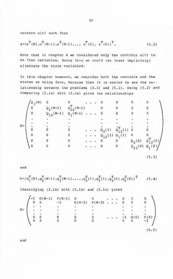
vectors u(t) such that

T T T T T T z =(x (N),u (N-1 ) ,x (N-1) , .. , u (0), X (0)) . ( 5. 2 )

Note that in chapter 4 we considered only the controls u( t ) to

be free variables . Doing this we could (at least implicitly)

eliminate the state variables.

In this chapter however, we consider both the controls and the

sta t es as being free, because then it is easier to see the re­

lationsh i p between the problems (3.1) and (5.1). Using (5 . 2) and

comparing (5.la) with (3.la) gives the relationships

B=

and

Ql ( N)

0

0

0

0

0

0

Identifying

0

Q2 (N-l)

Ql2(N-l)

0

0

0

0

0 T

Ql2(N-l)

Q1

( N-1)

0

0

0

0

( 3. lb) with ( 5. lb)

- I G(N-1) F(N-1) 0 0 0 - I G(N-2)

G=

0 0 0 0 0 0 0 0

and

0

0

0

Q2(1)

0 12(l)

0

0

0

0

0

" T 012(1)

Ql(l)

0

0

and ( 5. l e) gives

0 0 F(N-2) 0

0 -I 0 0

0

0

0

0

0

Q2 ( 0)

0 12(0)

0 0

G(O) 0

0 0

0

0

0

( 5. 3}

( 5. 4)

F ( 0) -I

( 5 . 5)

T T g=(O,O, ••. ,O,-xo>

63

( 5. 6)

where in (5.5), I is the nxxnx unit matrix. The constraints

(5.ld) determine the vector hand the matrix H in (3.lc) for the

CLQ- problem, but we can only write H explicitly when the

sequence t1

, t2

, .. ,tp in (5 . ld) is known .

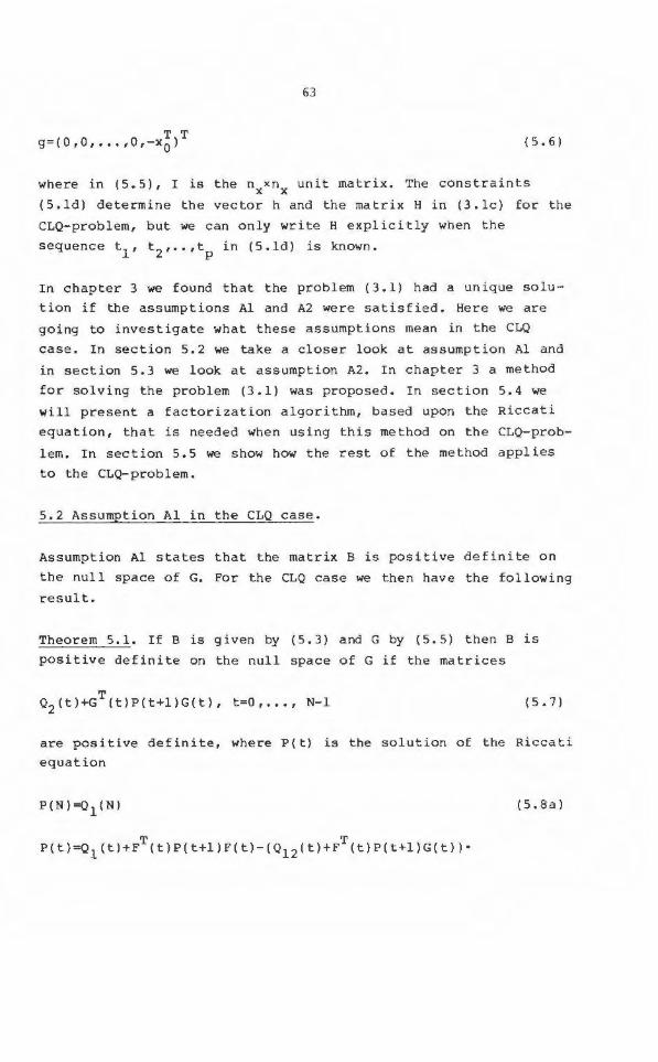
In chapter 3 we found that the problem (3.1) had a unique solu­

tion if the assumptions Al and A2 were satisfied . Here we are

going to investigate what these assumptions mean in the CLQ

case. In section 5.2 we take a closer look at assumption Al and

in section 5.3 we look at assumption A2 . In chapter 3 a method

for solving the problem (3.1) was proposed. In section 5.4 we

will present a factorization algorithm, based upon the Riccati

equation, that is needed when using this method on the CLQ-prob­

lem. In section 5.5 we show how the rest of the method applies

to the CLQ-problem.

5.2 Assumption Al in the CLQ case.

Assumption Al states that the matrix B is positive definite on

the null space of G. For the CLQ case we then have the following

result.

Theorem 5.1. If B is given by (5 . 3) and G by (5.5) then B is

positive definite on the null space of G if the matrices

Q2

(t)+GT(t)P(t+l)G(t), t =O , . .. , N-1 ( 5 . 7)

are positive definite, where P(t) is the solution of the Riccati

equation

(5.8a)

64

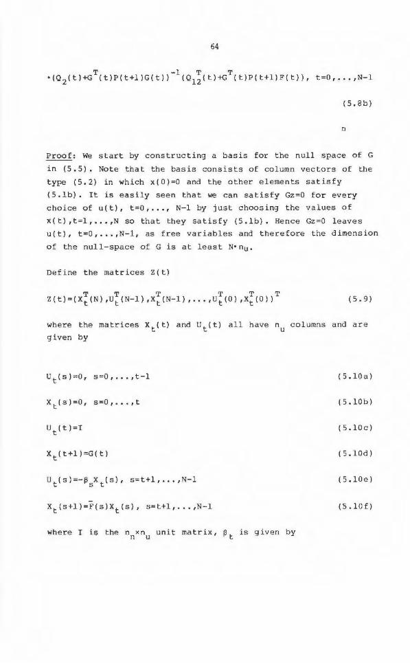
(5.8b)

0

Proof : We start by constructing a basis for the null space of G

in (5.5). Note that the basis consists of column vecto r s of t he

type (5.2) in which x(O)=O and the other elements satisfy

(5 . lb). It is easily seen that we can satisfy Gz=O fo r every

choice of u(t), t=O, ••• , N-1 by just choosing the values of

x( t) ,t=l, ••• ,N so that they satisfy (5. lb). He nce Gz=O leaves

u(t), t=O, ••• ,N-1, as free variables and therefore the dimension

of the null-space of G is at l east N•nu.

Def ine the ma tr ices z ( t)

T T T T T T z ( t) = c xt c N) , ut ( N-1) , xt c N-1) , ... , ut ( o) , xt ( o l ) ( 5. 9)

where the matrices Xt(t) and Ut(t) al l have nu columns and are

given b y

Ut(s)=O, s=O, ... , t-1 (5.lOa)

Xt(s)=O, s=O, ... ,t (5.lO b)

(5 .lOc)

(5.lOd)

(5.lOe)

xt (s+l )=F( s)Xt (s) , s=t+l, .. . ,N-1 (5.lOf)

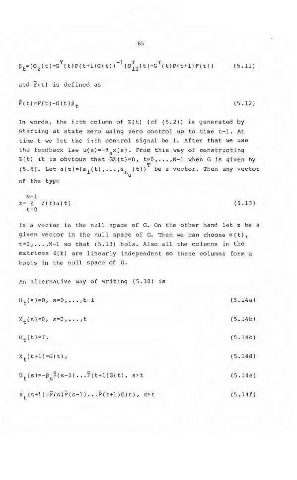
where r is the nnxnu un it mat r ix , ~t is given by

65

( 5 . 11)

and F(t ) i s de f ined as

F(t) = F{t )-G(t)~t ( 5 .12)

In words, the i: t h column of Z(t) (cf (5 . 2)) is generated by

starting at state zero using zero control up to time t-1. At

time t we let t he i:th control signal be 1. Afte r that we use

the feedbac k law u(s)=-~sx(s). From this way of cons tructing

Z( t ) it is obvious that GZ(t)= O, t=:O, . . . ,N- 1 when G is given by T

( 5 . 5). Let a: {t)=(a 1 (t), •.. , a nu{t)) be a vec tor . Then any vector

of the type

N-1 z= E Z(t)a(t}

t=O ( 5 .1 3 )

i s a vector in t he null space of G. On the other ha nd le t z be a

given vector in the null space of G. Then we ca n choose a:(t) ,

t =O, ... ,N-1 so tha t (5.1 3 ) hols . Also al l the columns in the

matrices Z(t) are linearly independent so these columns f orm a

basis in the null space of G.

An al t ernative way of writing (5. 10) is

Ut ( s)=O , s=O , ... ,t-1 (5. 14a)

Xt(s)=O , s= O, . . . ,t (5.14b)

{5. 14cl

X t ( t + 1 ) =G ( t ) I (5.14d)

Ut (s)=-~sF{s-1) . .. Ei(t+l)G(t), s>t (5. 14e)

- - -Xt(s+l)=F{s ) F(s - 1) .. . F(t+l)G(t), s>t (5 .14f)

66

I f z is given by (5.13) we have

N-1 N-1 zTBz= E E aT(s)ZT(s)BZ(t)a(t). (5.15)

t=O s=O

The term ZT(s)BZ(t) has the following property. From (5.3) and

(5.14) we have

-T -T -T -T T BZ ( t) = (X t ( N) , Ut ( N-1) , ••. , Ut ( 0) , Xt ( 0) ) ( 5 . 16)

where Xt(t) and Ut(t) are given by

xt (N)=Q1 (NJ °F(N-1) ••. r( N-1, ••• r( t+1 )G( t) (5. l 7a)

(5.17b)

x t 'P' = , Q 1 'P '-Q 12 , P) ~ p) r, p-1 , . .• r, p-1 > ••• 'F ( t + 1 , G, t > p>t (5.17c)

(5.17d)

(5.17e)

Ut(p)=O p< t (5 . 17f)

Xt(p)=O p~t (5 . 17g)

For s>t we then have

T T T T Z (s)BZ(t)= (Q12 (s}+G (s)P(s+l)F(s)-(Q2 (s)+G (s)P(s+l)G(s))~s)-

- -•F(s-2) . . . F(t+l)G(t)=O. (5 . 18)

For s=t we have

(5.19)

67

and for s< t we have

To obtain (5.18)-(5-20) we have used (5 . 8) and (5.11).

Hence (5 . 15) reduces to

N-1 zTBz= E aT(t)(Q

2(t)+GT(t)P(t+l)G(t))a(t)

t=O

( 5. 20)

(5.21)

and we finally conclude that zTBz> 0 if zfO and Gz=O and if

the matrices Q2 (t)+GT(t)+GT(t)P(t+l)G(t) are positive definite .

D

If the LQ problem (5 . la-c) was constructed to obtain a Newton

direction to the constrained optimal control problem (4 . 1 )­

(4 . 3), we have the following result.

Corollary 5 . 1 . The matrix vzz(O) given by (4.13) is positive de ­

finite if the matrices

are positive definite .

D

Pr oof: The statement follows from theorem 5 .1 and from theorem

4.1, which says that 6z(O) given by (4 . 10) is algebraically

identical to 6u(t), t=O, .•. ,N-1, which minimizes (4 . 20a) under

the constraints (4 . 20c) .

0

68

5.3 Assumption A2 in the CLQ case.

Assumption A2 is a constraint qualification for the quadratic

programming problem. In the CLQ case it is a l so c l osel y related

to the concept of controllability as will be shown later in this

section. For the CLQ problem, assumption A2 has the following

equivalent formulation.

Assumption A2: µi=O, i=l, ••. ,p and A.(t)=O, t=O, . .. ,N, is the

only solution of

i T A.(N)= E ~t.(h 1 (N)) (5.22a) id(N) 1

T i T O=G (t)f..(t+l)+ E µ.(h 2 (t)) ; t=O, .•• ,N-1 (5.22b) ie:I(t) 1

T i T A.(t) =F (t)A(t+l)H µ.(h1(t)) ,t=O, .•• ,N-1 (5.22c)

iEI(t) 1

where I(t) are defined by

I(t) = {i: t .=t} l

(c f (4.49)),

(5.23)

For the general case it is very diff icult to decide whether or

not (5.22a-c) have non-zero solutions in A. and µ. For some

special cases however it is possible to reformulate equations

(5.22) into a more practical condition. When there are no con­

straints at all we have the f ollowing resul t.

Proposition 5.1 . If there are no constraints of the type (5.ld)

defined by problem (5 .la-d) t hen the equations (5.22a-c) have

the unique so l ution A.(t)~O, t=O, •. ,N.

0

Proof. If we ha ve no constraints , then the sums in ( 5. 22) are

all zero. Hence (5.22a) gives A.(N)=O and (5.22c) shows that

69

A.(t+l)=O implies A.(t) =O. The proof then follows by induction.

0

Note that another way to formulate proposition 5.1 is to say

that the matrix G given by (5.5) has full rank .

If assumption A2 holds, then there exists at least one point

that satisfies the constraints. For the CLQ-problem it is ob­

vious that we have a feasible point of the constraints (5.lb)­

(5.ld) if the constraints (5.ld) are explicit functions of u(t)

and that we for allt could satisfy (5.ld) iEI(t) by just

choosing a proper u(t) . This fact suggests the following theo­

rem.

i Theorem 5 . 1 . If I(N)=~ and if for each t the vectors h 2 ,

iEI(t) are linearly independent, then A2 holds.

0

Proof. rrom (5.22a) and I(N)=~ we have A.(N)=O. Assume that we

have A. ( t)=O and µi =O, iEI(t) for t=N, .. . , p+l . By usi ng (5 . 22b)

for t=p we then get

( 5. 2 4)

But because the vectors h;,icI(p) are linearly indepe ndent ,

(5 . 24) implies µi=O, icI(p) . The equation ( 5 .22c) the n reduces

to

T A.(p)=r (p)A.(p+ll

X

But A.(p+l)=O and hence A.(p)=O.

The result then follows from induc tion.

( 5 . 25)

0

70

The most inte r esting case , however, is when we have some pure

state constraints, i.e. h;=o. In order to hand l e this type of

problem we conside r the co nc ept of controllability. We define

the t r.ansit ion matrix $(t,s), t~s, and t he controllability

ma trix W(t , s) , t> s , as

$(t+l,s} =F( t) $(t , s ) , t~s, $(s , s)=I

and

t - 1 W(t,s}= E $(t,p+l)G (p)GT(p)$T(t,p+l)

p=s

(5 .26}

( 5 . 27}

If we have only one constraint which is a s t ate constraint

relating to the time ti, the n we have t he following resul t.

Theore m 5.2. Suppose that we have only one constraint and that

h2

=0 for this co nstraint. Suppose also that W(t 1 ,t 0 J , defined by

(5.27) is nonsingular for some t 0 such that O~t 0 < t 1~N. Then A2

holds if hi,Fo.

0

Proof : From (5. 22) and (5.26) we have

i-. ( t) =O, t =t1

+1 , ... , N (5.28a)

(5 .28b)

and from (5.22b) we then ge t

(5.29)

This could also be written

(5.30)

71

where C is the matrix

( 5 . 31)

But CTC=W(t1,t

0). Hence, multiplying (5 . 30) by CT we get

( 5 . 3 2}

Because W( t1 ,t

0) is nonsingular and hilO , (5. 32) impl ies µ

1 =O

and from (5.28b) it follows that >-..(t) =O, t=O, . .. ,N .

0

If we have several s t ate constraints but they all relate to

different times, the following corollary follows from theorem

5. 2 .

Corollary 5 . 1 Let the times ti' i=O, ... ,p satisfy

O<t0

<t1

<... <t <N . If the matrices W(t. ,t. 1

J are nonsingular-- . p- ]. ].-and h~IO for i=l, .• ,p then A2 holds.

0

Now consider- the time invariant case with one t i me invar-iant

state constraint r-elated to each time.

The orem 5.3. Let the dynamics in (5.lb) be time invariant such

that F(t)=F and G(t)=G, t=O, ... , N- 1 and let the constraints in

(5.ld) be time invariant s t ate constraints such that

(5 . 33)

(h 1IO) where t .> n ,Vi and t.lt. if ilj . Suppose that the 1 - X l J

72

matrix C given by

n -1 - -- - X - T

C=(G,FG, ... ,F G) (5.34)

has full rank. Then A2 holds.

D

Proo f : Without loss of generality we assume that t.=n +i - 1. 1 X

Let k be the sma llest nonnegative integer such tha t

- k-h l ( F} GtO. (5.35)

That this k exis ts follows f rom (5.34) and the fact that C has

full rank and h1fO.

From ( 5. 22) we get

N - T s-t T A(t}= E µs -n +1 1Fx ) (h l ) ' n < t<N

s = t X x- - (5.36a)

N +l (FT}s-t(h l} T , A( t )= E µs-n O< t<n -1 - - X s=n X

X

(5.36b)

Now using (5.22b} f or t=N-k gives

- T - T - T T O=G A( N-k)=µN-n +lG (F )(h 1 ) ( 5 . 37)

X

The second equa l i ty follows from (5. 36) and the fact that

h1 (F)PG=O if p< k. He nce from (5 . 37) we have 11 N- n +l=O. Assume X

t hat µN 1

= .. . =µ 2

=0. Then us i ng this -nx + p -nx +

fact a nd (5.22b) for

t =p-k gives

( 5. 38)

which says that µ +l =O . Hence by i nduct ion we have µ. =O , p - n x i

73

i=l, ... ,N-nx+l , and from (5.36) it follows that

A(t) =O, t=O, .• ,N.

0

5.4 Factorization and the Riccati equation

As we have already mentioned, the problem (5.1) isa problem of

the type defi ned by (3.1). Therefore we can use the method pro ­

posed in chapter 3 to find the solution to (5 . 1) . When using

thi s method we need an efficient method for factorizi ng the

matrix o f (3.6) when B a nd G are given by (5 . 3) and ( 5.5) . We

will show here that such a factorization method is obtained when

the Riccati equation is solved . Therefore we first solve the

problem neglecting the cons t raints {3.lc), which in our case

corresponds to the constraints (5 . ld). We have already pre­

sented a method for finding the solut ion to the LQ-problem in

section 4 . 3 . 1. In this chapter we will aga in present the same

method but derive it in a diffe r e nt way. We do this for two

reasons . The first reason i s that we want to stress that solving

the Riccati equation is a factorization me thod and the second

reason is that it is easier to see what matrices define this

factorization . Hence consider the LQ-problem (5 . la)-(5 . lc). The

Lagrangian for t his problem is

T l T T L ( X , u , A ) =q l ( N ) X ( N ) + "2 X ( N ) Q l ( N ) X ( N ) +A ( 0 ) ( X O - X ( 0 ) ) +

T T +2 x (t)Q12 (t)u(t)+u {t)Q2 (t)u(t))+

H. T ( t + 1 ) ( F ( t) x ( t) +G ( t) u ( t) - x ( t + 1 ) } (5. 39)

If x(t), t=O , ... ,N and u(t), t=O, ..• ,N-1 is the solution to the

LQ-problem, then the Kuhn-Tucker necessary conditions state that

there exist multipliers ~(t) , t=O, . . . ,N such that 0 ~tt)=O,

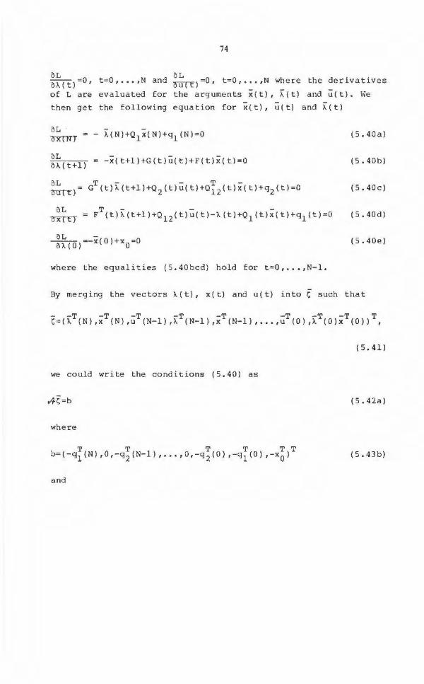
74

~~ (t)=O, t=O, .. . ,N and ~~(t)=O, t =O, ••• , N where the derivatives

of L are evaluated for t he arguments x(t), ~( t ) and u(t ) . We

t hen get t he following equat ion for x(tl, u(tl and ~(tl

bL oun:>

bL oxrn

-x(t+1i+G(t}u(tl+F(tlx(t) =o

where the equalities (5.40 bcd) hold for t =O, ••• ,N-1.

(5. 40a)

(5. 40b)

( 5. 40c)

(5.40d)

(S.40e)

By merging the vectors A(t) , x(t) and u (t) into ~ s uc h that

- - T -T - T -T -T -T - T - T T ' = (A (N),x (N),u (N- 1),A (N-1),x (N- 1), .•. ,u (0),A (O)x (0)),

(5.41)

we could write the conditions (5.40) as

(5.42a)

where

T T T T TT b = (-q1 (Nl , o ,-q 2 (N- 1) , •. • , o ,-q 2 (O l ,-q 1 co l , - x0 l ( 5. 43b)

and

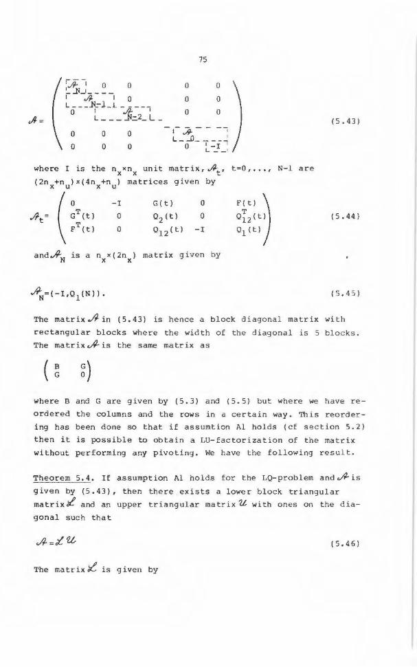
~ -, 0 0 '- ... l'U ___ _ I,/}. IQ L ____ N:-.LL _ ----

0 I .fl- t L ___ .ll=.2_ L _

0

0

0

0

0

0

0

0

0

75

0

0

0

where I i s the n xn X X

unit ma tr ix, .fi-t,

(2nx+nu)x(4nx+nu ) matrices g i ven by

( ~T(t) -I G(t) 0

/1 = 0 Q2(t) 0 t FT(t) 0 Ql2( t) -I

~=(-I,Q l (N}} .

(5.43)

t=O I •• • I N-1 are

F(t) ) or2(t) ( 5 . 44)

Ql(t)

( 5 . 45}

The matrix./1-in (5.43) is hence a block diagonal matrix with

rectangular block s where t h e width of the d iagonal is 5 blocks.

The matrixA-is the same matr ix as

( ~ ~) where B a nd G are given by (5.3} and (5.5) but where we have re­

ordered the co lurnns and the rows in a certain wa y . This reorder­

ing has been done so that i f ass umtion Al ho lds (cf section 5 . 2)

then it is possible to obtain a LU-factorizat ion o f the matrix

withou t performing any pivoti ng . We have the following result .

Theorem 5 . 4 . If assumption Al holds for the LQ- pro blem and A- is

given by (5 . 43), then t here e x ists a lowe r block triangular

matrixi' and an upper triangular matrix U with ones on the dia­

gonal suc h tha t

( 5 . 4 6)

The matrix :L is given by

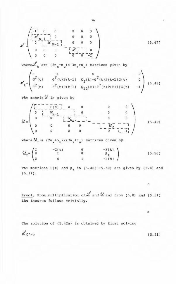
1-=-1-, 0 0 I I Id[- - -, 0 L - ..N;:l.-' - - 1

O I ~ N- 2 -----L 0 0 0

0 0 0

0

0

0

0

0

0

76

0

0

0

-,~ ---, 0 L_...Q __ L _ _

0 0 - I I L_...J

-I GT(t) P (t+l)

0

Q2

(t )+GT(t}P(t+l)G(t)

FT(t) P ( t+l) 012 (t)+FT(t)P(t+l)G(t)

The matrix ?L is given by

0

0

where Utis

U,· (:

0

0

0

0

0

0 - , I

0

0

(2n +n )x(3n +n ) matrices X U X U

-G ( t) 0 I 0

0 I

0 0

0 0

0 0

-u- - --, - .0.. - - -1 0 I_ _ ~I

given by

- F(t) ) ~t

- P(t)

( 5. 4 7)

~) (5.48) -I

(5.49)

(5.50)

The mat rices P(t) and ~t in (5.48)-(5.50} a r e given by (5.8) and

( 5.11).

0

Proof. From multiplication o f X and U and from (5. 8} a nd (5.11)

the theorem f ollows t rivially .

0

The sol ution of (5. 42 a} i s ob t ained by firs t solving

( 5. 51)

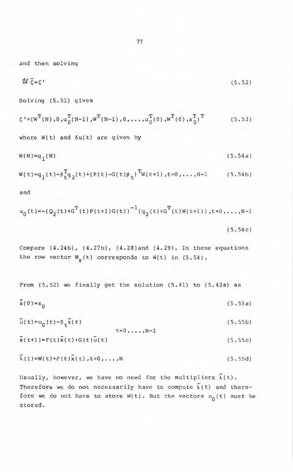
77

and then solving

U ~=C' ( 5 . 52)

Solving (5.51) gives

I T T T T T TT c =(W (N) , O,u o (N-1),W (N-1), 0, .. • ,u o (O ) , W (0), x o) ( 5. 53)

where W(t) and öu (t) are given by

W(N )=q l (N) ( 5 . 54a )

w ( t) =q 1 ( t >-f3 ~q 2 ( t) + ( F ( t > - G ( t) f3 t) Tw ( t+ 1) , t=O , .. . , N-1 ( 5 . 54b)

and

(5 . 54c)

Compare (4 . 24b), (4.27b), (4.28)and (4.29). In these equations

the row vector Wx(t) corresponds to W( t) in (5 . 54) .

From (5 . 52) we final ly get the solution (5 . 41) to (5 . 42a) as

(5.55a)

( 5 . 55b)

t =O, . •. , N-1 - - -x(t+l)=F(t)x(t)+G(t)u(t) ( 5. 55c)

~(t)=W(t) +P(t)x(t ) ,t=O, .. . ,N (5.55d)

Usually, however , we have no need for the multipliers A(t).

Therefore we do not necessarily have to compute ~(t) and there­

fore we do not have to store W(t) . But t he vectors u0

(t) must be

stored.

78

When we examine the equations (5.54} and (5 . 55) we find that the

factorizat ion of ,fl- in (5.42} is defined by the matrices

G(t) ,F(t} ,Q2

(t)+GT (t)P(t+l)G(t) and ~t if we do not need ~(t) .

Hence we now have an effective method to factorize the left hand

side matrix in (3.6} in the LQ-case. Also, we know how to find

the solution z to (3.6} in this case,

5.5 Inequality constraints.

We are now r eady to hand l e the inequality constraints (5 . ld) . In

the method proposed in chapter 3 we need to calculate the matrix

z in (3 . 5) which is the solution to (3 . 7). We also need to cal­

culate µ. which is the solution to {3 . 8}. Hence we also need to

calculate the matrix A in (3 . 9) and the vector d in (3 . 10).

Without any loss of generality we assume that the first p ' of

the constraints (5.ld) are in the active set. Now we use Remark

3.1 to calculate the i : th column in z (3 . 5).

Hence in the vector b given by (5.42b) we replace q2(ti) and

i i q 1 {ti) by h 2 and h1 • All other elements in bare set to zero and

the resulting vector is called bi. Let the i : th columns of Z a nd

A be s tored in r. i wi th the same structure as ind icated by

( 5 .41). Then we get this i;:. as the solution to l

;/r.•. =b. l l

Ur. .=r. ~ l l

{ 5 . 56a)

(5.56b}

where <.i has the same structure as (5.53) . Comparing wi th (5.54)

we see that the solution to (5.56a) is

Wi (t} =O , t=ti+l, ••• ,N (5.57a)

79

u.(t)=O , t=t.+l, ... ,N l l

(5 . 57b)

(5.57c)

( 5 . 57d)

W . ( t ) = ( F ( t ) - G ( t ) Il t) 'rw . ( t + l ) , t = 0 , • . . , t . -1 , 1 l l

(5 . 57e)

T - 1 T Ui(t) =- (Q2 (t)+G (t)P(t+l)G(t)) G (t)Wi(t+l),t=O, ••• ,ti-1.

(5.57f)

and if we compare with ( 5. 55 ) we see that the solution to

(5 . 56b) is

x i ( 0) =0 ( 5 . 58a)

(5 . 58b)

t=O, •.. ,N-1

X i ( t +l) = F ( t) X i ( t) +G ( t) LI i ( t) , ( 5 • 5 8 C)

where in (5. 57 ) and (5.58) the subscript i i ndica t es the i:th

c olumn of z.

The e l ement aij in the matrix A in (3 . 9) is given b y

i i -a .. =-H1

x.( t .J-h2 u.(t. ) . (5 . 59) l] J l J l

The element di in the vector d in ( 3 . 10 ) is given by

where x(t) and u(t) is given by (5 . 55) .

We t hen know all quantities that are needed to solve (3 . 8) to

obtain µ . . The complete solution to the CLQ- problem is

p ' x(t ) =x{t)H Jl ~X. (t} ,t=O , ••• , N

i=l 1 1

80

p' u(t} =u( t }H µ(ui(t),t =O, .•• ,N -1.

i =l

(5. 6la)

( 5. 6lb)

This is of c o u r se true only i f we have chosen the correc t se t o f

act i ve constraints . Otherwise we have to f i nd a nother set of

active constraints accord ing to the rules g iven in section 3.

By substituting u(t) and ui(t) in (5. 6lb ) and using (S.55b) and

(5.58b) we get

p' - p'_ u ( t ) = uo ( t ) - ~ X ( t ) + L µ ! ( u . ( t ) - ~ t X . ( t ) ) = uo ( t ) + L µ ! u i ( t ) -

t i=l 1 1 1

i=l 1

p' - p ' _ - ~ (x( t ) +L µ! x. (t)}=u

0(t}H µ!u. (t} -~tx(t)

t i =l 1 1 i =l 1 1 ( 5. 62)

where the last equality follows f rom (5.6 l a}. There f ore we can

choose to store ui(t} i nstead o f ui(t) a nd xi(t}. Instead of

( 5. 61} we then use

p ' u(t)=u

0(t)H 'µ • . u . (t)- ~ tx(t)

i =l 1 1

x(t+l)=F{t)x(t)+G( t) u(t)

t=O, ..• ,N-1

(5 . 63a)

(5 . 63b)

( 5.63c}

However, in order to be able to calculate the e lements a .. given l]

by (5. 59) we have to calcul a te xi(t) a nd ui( t ) but we need not

necessari ly store them. In the first iteration of the method

proposed i n chap t er 3 we know whi c h cons t ra ints belong to the

ac tive set. We can therefore use (5.59} t o ca l culate all e l e­

ments i n A.. However, in later ite ra t ions when a new constraint

is added to the act i ve set, we cannot use (5 .59) f or all ne w

elemen t s if we do not want to reca lcula te xi(t} and ui(t) for

a lready active cons traints. Only the elements i n the new column

in A could be obtained from (5 . 59) . But then we ut i l i ze the fact

81

that the matrix A i s symmetric , and therefore also the new row

could be calculated without storing the values xi(t) and ui(t)

for already active constraints.

82

83

6 REGULARIZATION ISSUES

6.1 Introduction

In chapter 4 we discussed how to determine a Newton direct ion in

the space of control actions for the optimal control problem

(4.l)-(4.4). Th is was achieved by solv ing the quadratic sub­

problem (4.53) . For this sub-problem to have a unique solution

we introduced the sufficient assumptions Al and A2 dealing with

positive definiteness and linear independence respectively. In

the previous chapter we discussed how to test whether these

assumptions are satisfied.

However, even if these assumptions are satisfied at the optimal

solution to the posed problem , it may happen that they are vio­

lated for some sub-problem that we encounter dur ing the i tera­

tive search for t he solution . In this chapter we shall briefly

discuss how the sub-problems can be modified so that the suf­

ficient cond itions Al and A2 are assured to be satisfien for all

subproblems that arise during the iterative procedure . In sec­

tion 6.2, assumption Al is treated, while assumption A2 is dis­

cussed in section 6 . 3 . When nothing else is explicitly stated,

we shall use the same notation as in chapters 2 and 4 .

6.2 Regulariza tion of matrices (Assumption Al)

The assumption Al requires that the Hessian of the Lagrangian is

positive def ini te on the orthogonal complement to the space

spanned by the gradients of the equality constra ints. When app­

lied to an unconstrained optimization problem this simpl y means

that the Hessian of the objective function should be positive

definite . If this is not the case then Newton's method is un­

suitable for the numerical search, since it does not generate

descent directions . A very natural and common way to handle that

situation is to add a matrix to the Hessian so that the resul­

ting matrix is positive definite (see e . g. Luenberger (1973), p .

157). This idea was proposed by Levenberg (1944) and Marquardt

( 1963) . Here we shall describe two basically different choices

of such matrices, and how to adapt the Levenberg-Marquardt

84

method to our particular problem. The two cho ices in question

are:

Cl : µI where µ~O and I is the unit matrix

C2: A non-negative diagonal matrix D.

These methods are also described in Fletcher (1980). The choice

Cl may be motivated in the following way:

Assume that we want to solve the problem

minimize J.(z) ( 6 . 1)

( cf ( 2 • 11 ) ) •

Newton's method for this problem then generates search direc­

tions which are the solutions to

( 6. 2)

If J.zz(zk) is positive definite and the Taylor series is

adequate in a sufficently large region around zk, then this

should give a reasonable decrease in the objective function.

However, if J.zz(zk) is indefinite then the expression (6.2) has no lower bound and the problem has no bou nd ed solution. A

possible way to modify this problem is to res trict the search

for a new va lue to a small enoug h region around the previous

iterate:

min imize dk

subject to

(6 .3a)

(6. 3b)

here Ek is a properly chosen pos i tive scalar. The Lagrangian for

the problem (6 . 3) is

( 6. 4)

85

and the Kuhn-Tucker conditions for this problem are

{ 6 . Sa)

{6.Sb)

( 6 . Se)

{6 . Sd)

If the constra i nt (6.3b) is active, the solution to the problem

( 6 . 3) is

( 6 . 6)

whe re µ is chosen so that jak l =ek· However , any choice of µ such

that the matrix

( 6. 7 )

is positive definite will make dk given by (6 . 6) a descent

direction. Therefore , in practice the variable ek is neve r

explicitly given. Rather, µis chosen so that the matrix ( 6 . 7 )

is positive def i nite . When µ tends to infinity, this direc t ion

tends to the steepest descent direction. This means that too big

a value of µ may a give slow convergence rate .

The choice C2 is motivated by the following idea from Gill ,

Murray and Picken (1972). The idea is to make a UTU- factoriza ­

tion of the modified matrix :

{ 6. 8)

The elements of t he diagonal ma t rix Dk are chosen in the course

of t his factor i zation so that the right hand side of ( 6 . 8) is

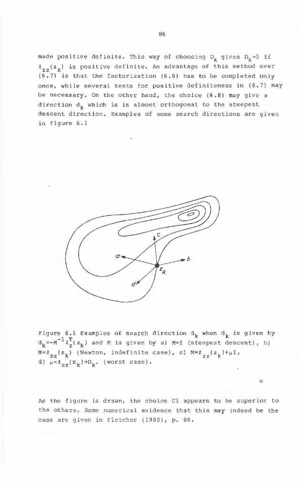
86

made posit i ve definite . This way of choosing ok give s Dk=O if

~ (zk) is positive defi n ite. An advantage of this rnethod over zz (6 . 7) is tha t t he factorization (6.8) has to be completed only

o nce , while several tests for posi t ive defin iteness in (6.7) may

be necessary. On the other hand , t he choice (6.8) may give a

d irection ak which is i s almost or thogonal to the steepest

des c e nt direc t ion. Examples of some search directions are given

in figure 6.1

Figure 6.1 Exampl es of search d i rection dk when d k is g iven by -1 T dk=- M t

2(zk ) and M is g i ven by a) M=I (steepest descent), b )

M=t (zk) (Newton, indefinite case ), c) M=i (z k )+µI, zz zz d) µ=t

22(zk)+Dk . ( worst case) .

0

As t he figure is drawn , t he choice Cl appears to be s uperior to

the others . Some numerical evidence that t h i s may i ndeea be the

case are given in Fletcher (1 980), p. 88.

87

Let us now con sider the optimal control problem (4 . 1)-(4 . 4) . We

found in section 4.3.l that the Newton step for the unconstrain­

ed optimal control problem is given by (4 . 10) :

where V(t) is g i ven by (4 . 8) and 6z(0) is the increment in u(t),

t=O, .. . ,N- 1. (see equation (4.6)), Now, if Vz2

(0) is not posi­

tive definite, then we modify it using either of the choices Cl

o r C2. Comparing with equation (4 .14g) we find that the choice

Cl corresponds to adding µI to the matrices iuu(t) , t=O, . .. , N-1

and the choice C2 to adding D( t) to J.uu ( t) where D( t) are non­

negative diagonal matrices . From corollary 5 . 1 we know that we

can check if the resulting matrix is positive definite just by

investigating the matrices

( 6 . 9)

where Wxx(t+l) is the solution to the Riccati equation

(6 .lOc)

+V (t+l)f (t)+fT{t)W (t+l)f (t)) • {.t (t)+D(t)+V (t+l)f (t)+ X XU X XX U UU X UU

+fT{t)W (t+l)f (t))-l•(J. +V {t+l)f (t)+fT(t)W (t+l)fx(t)) U XX U UX X UX U XX

(6.lOd)

88

We have written these equations here for the choice C2. In the

c ase of Cl we just replace D(t) with µI. Notice tha t the choice

Cl requires µ to be equal for all the N time instants .

Therefore, using the choice Cl we may have to solve t he Riccati

equation (6.10) several t imes before a proper va l ue of µ is

fo und. In the case of C2, however , the matrices D(t) can be

found on-line, by solving (6.10) only once per iteration.

There fore the choice C2 will be used in our a l gori t hm for the

optimal control probl em, despite the possible disadvantage indi­

cated i n figure 6.1.

It is i n te res ting to note t hat add i ng the ma trix D ( t) to ,t uu ( t l may be in terpre ted as add i ng the t erm

1 T 2

( u ( t) - uk ( t) ) D ( t) ( u ( t) - uk ( t) ) ( 6 . 11 )

to the cost- f unct ions t(x(t) ,u(t) ,t) in the performance index

(4.3), where uk(t) is the cu~rently used control signal. Adding

such a t erm is very sim.ilar to t he convergence control parameter

(CCP) technique proposed by Järmark (1977), for continuous time

optimal control problems. I n the original CCP-method, however ,

the same matrix is used at every time i ns t ant , and the choice of

the matrix is determined by the decrease in the cost function

between iterations. From this discussion it may co nsequently be

concluded tha t t he CCP-technique may be interpreted as a

Levenberg-Ma r q uardt method .

Hence when we use the choice C2, we repl ace t he matrices Quu(t) by

Q ( t) =Q (t)+Dt uu uu (6 . 12)

when solving (4. 53). In the followi ng when we consider th i s

formulation instead of (4. 53) we will call it "the regu l arized

CLQ- problem".

89

6 . 3 On assumption A2.

The assumption A2, that the gradients of all the constraints be

linearly independent, is actually stronger than necessary. The

algorithm given in chapter 3 will work well as long as the rows

of G and H are linearly independent throughout t he computa tions,

where H contains t he rows corresponding to the active const ­

raints (3.lc). lf, during the computations, the active const­

raints become linearly dependent, there are four, conceptually

different , possible causes for this:

Rl . There exists no point that satisfies all the constraints

( 2. llbc) .

R2 . The constraints are linearly dependent at the optimum.

R3 . There e xists no point that satisfies the constraints

in the quadratic s ub-problem (2.15) even though (2 . llbc)

have feasible points.

R4 . The constraints (2 . 15bc) have feas ible points, but whe n

solving the quadratic subproblem (2 . 15), the algorithm uses

so many active constraints that they become linearly

dependent .

The first two reasons depend on the actual problem only, and

there is nothing that the algorithm can do about it. The

fol lowing exam(?le illustra tes how R2 may happen:

Example 6 . 1 . Consider the problem

minimize

-z < 0 2-

90

The solution to this pr:oblem is z= ( ~) . At th is point however: ,

the co nstraints have the derivatives (0,1) and (0 , -1) , respec­

tively, which are linearly dependent.

0

The possibilities R3 and R4 of course also depend on the p r oblem

but t hey also depe nd on the starting point given to the algo-

ri thm, and o n how the algorithm chooses the active constraints

among the i nequali ty constraints. We illustra te R3 wi th the

following example.

Examp le 6.2. Assume that we have two variables only , z1

and z 2 ,

and that we have two nonlinear eq uality constraints g1

(z)=O and

g2

(z) =O . Assume also that we have simple bounds on the variables

such that

-l<zi ~l, i=l , 2 (6 . 12 )

and that the cons traints have a feasible point strictly inside

this box. If the point zk is t oo far awa y from this feasible

point it may happen that the l inearized constraint g(z)=O has no

solut i on inside the box (6 . 12). See Pigure 6.2 .

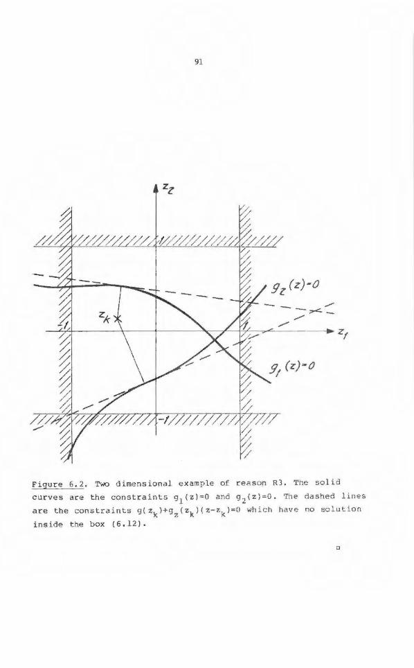
91

Figure 6 . 2. Two dimensional example of rea son R3. The solid

curves are the constraints g1

( z )=O and g 2 (z);;Q. The dashed lines

are the const r ain ts g (zk) +g2

(zk)(z-zk) =O which have no solution

inside the box (6.12).

D

92

A remedy f or R3 has been proposed by Powell (1977). His idea is

to scale all equality constraints and all violated inequality

constraints so that they will have a f easible solution close to

zk. Then the nonviolated inequality constraints should not,

hopefully, be activa t ed during the iteration in question.

Therefore a little step could be taken towards a feasible point

of the nonlinear constraints. The choice of the scaling f actor,

mentioned above, has been f urther studied by Tone (1983).

The possibility R4 may occur when there are more active con­

s traints than free variables. Therefore, in order to avoid that

R4 occurs , the technique for choosing active constraints when

solving the quadratic problems (2.15) should be designed so that

the number of active constraints is kept small throughout the

calculations. A strategy fo r selecting the active set, t hat usu­

al ly gives fewe r active constraints than the strategy described

in section 3.2, is given in Goldfarb and Idnani (1983). They use

the strategy of section 3.2 applied to the dual problem to

(2.15).

93

7. CONVERGENCE OF THE OPTIMIZATION ALGOR ITHM

7 . 1 Introduction

So far we have only eons idered the problem of f ind i ng a proper

direction when ite ratively solving t he nonlinear constrained

programming probl em {2 . 11). We have said nothing about how to

choose the value of cxk in (2 . 12). This choice is very important

for the convergence of the algorithms proposed earlier.

The discussion o f convergence is usually divided into two con­

cepts, namely global convergence and local convergence . When we

investigate g lobal convergence for an algori thm, we f ind the

conditions under which the algorithm converges to a Kuhn-Tucker­

point from an arbi trary starting point. This Kuhn - Tucker- point

might not even be a local minimum point, but to prove conver­

gence to a local minimum point from an arbitrary starting point

seems to be a very complicated task .

Whe n we talk about local conve rgence , we es timate the speed of

convergence close t o a local minimum point . The speed could for

instance be linear , superlinear or quadratic .

When we derived o ur algori t hm for constrained optimal control

problems , we did that by interpreting it as a nonlinear pro­

gramming problem . Therefore, all convergence i:-esul ts obtained

for Wilson ' s method or Quasi-Newton versions of Wilson ' s me thod

can be applied to our algorithm. Accord ing to Ohno (1978) no

proof of convergence has been presen t ed for the Mayn e (1970)

algorithm or ·analogus second order algorithms e . g . {Jacobson

(1968), Dyer and McReynolds {1970)) . Howe ver , Ohno {1978) proved

that his algorithm for solving cons trained optimal control

problems converges to a Kuhn-Tucker point.

In section 7.2 we give some rules for choosing the s t ep-length

for unconstrained problems and in section 7 . 3 we discuss const­

rained problems . We t hen use the Watchdog technique , given in

Chamberl ain et al (1979), for the constrained opt imal control

problem and give proofs for both global and local convergence

94

in this case. In Section 7 .4 we prove global convergence and in

Section 7 . 5 l ocal convergence.

7 . 2 Step leng th r u les for unconstrained optimization.

The basic idea of step length rules is the following. We assume

tha t we have the problem (2.11) but without constraints. Then

the problem reduces to

minimize !(z) ( 7 .1)

We also ass ume that with some method (for ins tance the Newton

method or the steepest descen t method) we have found a descent

direction dk, i.e. !2

(zk) • dk <O. Now we wa nt to determine ak i n

the formula

so that zk+z* (i .e . the solution of (7. 1 )) when k+m . The mo s t

obvious way to choose ak i s to minimize !(zk+l). Hence

cxk=arg min !(zk+adk) ex

This method is, however, usually not feasible to use in

practice , since it requires a lot of function evaluations.

(Luenberger (1973) p. 147).

( 7. 3)

Thcrefore we must accept rules for choosing cxk which do not make

!(zk+l) as small as p o ssible. However , to acc ep t cxk as s o on as

the criterion

( 7 . 4)

is s atisified, is not sufficient, because then the seqence

{zk] may converge to a point z for wh ich ! 2 {z)~O. Goldstein

and Ar mijo have proposed rules for choosing cxk in ( 7 . 2) such

that {zk} converges to a poin t z for which !2(z) =O. See pp. 20-

21 in Bertsekas (1982} for deta i ls of these me thods and o the r

rules for choosing the step-size.

95

7 . 3 Step length rules for constrained optimization .

When we have constraints in (2.11) we must not only pay atten­

tion to the value of ..t(zk+akdk) when we choose the parameter ak'

but also to the violations of the constraints . We must,

therefore, choose ak to obtain a suitable balance between the

decrease (or increase) in the object1ve function .t ( z) and how

well the constraints

g(z)=O ( 7. Sa)

h( z )2_0 (7 . Sb)

are satisfied at the point zk+l'

This balance is usually achieved by constructing a cciterion

function which is the swn of the ob jective function .t ( z) and a

penalty term to the constraints (2 . llbc). For examples of such

criterion functions, see Powell (1977) and Han (1977) . The

method for choosing the step-length a, for which the strongest

convergence resul ts hol ds, is the wa tchdog techn ique given by

Chamberla i n et al. ( 1979). In the next section we will apply

that method to the optimal control problem .

7.4 Convergence for the constrained optimal control problem.

In section 4 .1 we defined the constrained optimal control

prob l em by (4.1)-(4 . 4).

X ( t + l ) = f ( X ( t) I u ( t) , t) I t =O , ..• I N-1

N-1 J(u)=..t(x(N) ,N)+ E ..t(x(t) ,u(t) ,t)

t:O

h i (X ( t. ) I u ( t. ) ) <O I i =l , •.. I p l 1 -

( 7 . 6a)

(7 . 6b)

(7.6c)

( 7 . 6d)

96

The problem is to minimize J(u) in (7.6c} when the constrain t s

(7.6ab) and (7 . 6d} are satisfied. The Kuhn-Tucker necessary

conditions for a solution to this problem is t hat there must

exist multipliers A and µ s uch that the f ollowing conditions are

satisf ied:

(7.7a}

(7 . 7b)

~ (t)+y (t)+AT(t+l)f (t )=O u u u

( 7. 7c)

µ~O (7.7d)

(7.7e)

(for defeninition of y( t ) see eq . (4.50)) as well as the condi­

tions (7. 6a) , (7 . 6b ) and (7. 6d) . When we talk about a Kuhn­

Tucker-point for the problem (7.6) in the following we mean

u (t), A(t) and µ such t hat these conditions are satis f ied.

We assume that we use Newton' s method in the control space for

solving problem (7.6). We th e n get a s equence {zk (O)} (cf (4.6))

which hopeful ly converges to a local minimum point (4. 1 )-

( 4 . 4).

The sequence {zk(Ol } is def ined b y

( 7. 8)

where 6z(0) is given by the solution to t he constrained linea r

quadratic optimal con trol problem (4.53). When solving th is

problem we assume that the regulari za t ion technique p roposed in

sect ion (6.2) is used.

Here , we will use the Watchdog technique as described in

97

Chamberlain et al (1979) for choosing the value of ak in {7 . 7).

We start by defining two criterion functions JP( u) and JL(u) as

p i J L { u I µ ) =J ( u ) + E µi h ( X ( t i ) I u ( t i ) )

i=l

(7.9a)

(7 .9b)

where J{u) is given by (7 . 6c) and µi in (7.9b) is the Lagrange

multiplier of the constraint i. The f unction JL(u,µ) is

actually the Lagrangian to the problem (7 . 6) . This is the reason

for the subscript Lin JL(u) . The subscript Pin J p{u) stands

for penalty. We assume that the constants µ.,i=l, .. . ,p have been l

chosen so that

( 7 .10)

at each iteration . The multiplier µk is obtained when solving

(4.53) at iteration k and ( µk ) i is the i : th component of this

multiplier. We now define the follow i ng two cdteria .

Cl: (7 .11)

1 where oE(O,~) and 6Jkz is given b y

N-1 6J k = ..l { N ) 6 X { N ) + E ( .R. ( t) 6 x ( t ) H ( t ) 6 u ( t )) +

Z X t =O X U

p . . . l l - 1 + E ( h { t . ) 6 x ( t . ) +h ( t . ) 6 u ( t . ) ) • µ . • I { h ( t . ) > 0)

i=l X l l U l l l 1 { 7 . 12)

Here 6u{t) is generated by the solution to (4.53) and öx (t) is

the solution of the difference equation

6 X ( t+ l) =f X ( t) LI X ( t) +f u ( t) ll u ( t) , t=O I •• , N-1 (7.13a)

6x(0)=0 ( 7 . 13b)

98

I(T) is an i ndicato r function which is one if the condi tion T i s

true and zero otherwise . Note that 6Jkz is the directiona l

deriva tive of JP (uk) i n t he d irection 6z(0) .

The other criterion is:

(7.14)

Let ~E ( O , l) and let s be a posit i ve integer. The watchdog

technique is now given by the following scheme.

Step 0 : Let a c ontrol sequence u0 be given . Set k=O and

w=Jp(u 0 ) . Calculate 6z(O) given by the solution to

(4.53) for this control sequence .

Step 1 : Let ak=~j where j is t he smallest nonnegative in t eger

such that at leas t one of t he criteria Cl and C2 is

sa tisfied . Put uk+l=uk+ak6z(0} and go to step 3.

Step 2: Le t ak=~j where j is the smallest nonnegative i nteger

such t hat criterion Cl is satisfied . Put

uk+l=uk+ak6z(O ).

Step 3: Calculate 6z(O) for the control sequence uk+l . If

JP(uk)~w , set r=k,w=Jp(uk) and v=JP(u k )+aa k6Jkz "

S t ep 4: Put k=k+l. I f JP(uk)~v go to step 1 , and if v<JP(uk)~w

go t o step 2.

Step 5: If k-s~r go to step 2. Otherwise set uk=ur and r=k and

then go to step 2 .

If we have no constraints of the type (7.6d ), t his method

r educes to the Armijo step size rule.

The reason for using t~~ criterion functions i s that using only

c ri terion Cl may prevent superlinear convergence of the sequence

{zk} and using only the cr iterion C2 , t he seque nce {zk} may

converge to a point t hat is not a Kuhn-Tucker point.

99

The global convergence of this algorithm is assured by the

following t heorem.

Theorem 7.1. (From Chamberlain et al. (1979)). Let {uk} be given

by the wa tchdog technique and assume that the pred icted decrease

AJ kz is bounded away from zero if uk is bound e d away from a

Kuhn -Tucker poi n t. Then, if JP ( uk) is bounded below , the

seq uence {uk: k=O,l, . } hasa limit point which isa Kuhn-Tucker

point.

0

Proof : See Chamber l ain et al. (1979) .

0

That LIJkz is bounded away from zero if uk is bounded away from a

Kuhn-Tucker-point in our algorithm follows from the following

theorem .

Theore m 7.2. If for all k the subproblems (4.53a) sat i sfy t he

assumptions Al, explained in section 5.2, and A2 explained in

section 5 . 3, then AJkz is bounded away from zero if uk is not a

Kuhn-Tucker-point of (4 .1 ) - (4 . 4) . This result holds also if t he

reg ularization method proposed in section 6.2 is used .

0

Proof. Let the row vectors A(t) satisfy

A(N) =.l (N)+ I: (µk) .hi(N) X iEI(N) 1 X

(7 .15a)

>..(t)=.l (t)H(t+l)f (t)+ I: (µk) .hi(t)-x X iEI(t) l X

-( .l (t)H(t+l)f (t)+ I: (µk) .hi(t))l3t U U iEI(t) lU

(7.15b)

where µk are the Lagrange mul tipliers obtained when solving the

k:t h quadratic subproblem (4.53). Using (7.13a) we get the

equality

100

0=-A(t+l)Ax( t +l)+A(t+l ) f (t)tix(t)+A(t+l)f (t)tiu(t) X U

( 7 . 16)

If we for- t=O, ... ,N-1 add (7.16) to (7.12) we get

tiJ k = (.t (N)-A(N)+ E µ.hi(N)I(hi(N}>O))Ax(N)+ z X iEI(N) l X

N-1 + E {(1 (t}+A(t+l)f ( t }-A(t))Ax(t)+(i (t)+A(t+l)f (t))tiu(t}+

t=O X X U U

+ E µi(h!(t)tix(t)+h~(t)tiu(t))I(hi(t)>O)}= iEI ( t )

=(.tx(N)+ E (µk) .hi(N)-A(N)+ iEI(N) 1

X

+ E (µ.•I(hi(N}>O)-(µk) .)hi(N))tix(N)+ iEI(N) l l X

N-1 . + E {(.t (t)H(t+l)f (t)+ E (µk) .h 1 (t) - A(t))Ax(t)+

t=O X X iEI(t) 1 X

+(.t (t)H(t+l)f (t)+ E (µk) .hi(t))tiu(t)+ u u iE I (t) l u

+ E (µ1. •I(hi(t)>O)-(µk) .)(hi(t)tix(t)+hi(t)tiu(t))}

iEI(t) l X u

Now, Au(t) is given by the solution to the guadr-atic subpr-oblem

(4.53). Using (5.62) we can then wr-ite tiu(t) as

tiu(t) =öu(t)-~ttix(t)

and using (7.15) we get

- i i /:;J = E (µi I ( h ( N )> 0) - ( µ k) i) h X ( N) ) /:; x ( N) +

zk iEI(N)

N-1 · + E {Cl (T)+A(t+l )f (t)+ E (µk) .h

1(t))öu(t)+

t=O u u iEI(t) 1 u

101

- i i i + E ( µ . I ( h ( t )> 0 ) - ( µ k) . ) ( h ( t) !::. X ( t) +h ( t) 6 u ( t) } iEI(t) 1 1 X u

( 7 .1 7)

Using the fact that t::.x(t) and t::.u(t} satisfy the constraint

(4.53d) we have

( 7 .18)

i If h (ti)>O, then the left hand side of (7.18} must be negative,

and using (7.10) we obtain

( 7 .19)

If hi(t.)<0 and (µk).>0, we have equality in (7.18) and the 1 - 1

inequality (7 .19) is again obtained . Hence the inequality (7.19)

holds for all i, and from (7.17) we get

N-1 t::.J < E (.R. (t)+A(t+l)f (t)+ i: (µk) .hi(t))ou(t)

zk- t=O u u iEI(t) 1 u (7.20)

Comparing (4 . 53) and (5.1) and then using (5.62) we obtain

öu(t}=-C-tl(.R. (t)H(t+l)f (t)+ E (µk) .hi(t))T u u iEI(t) 1 u

( 7 . 21)

~ T ~ Here Ct is the matrix Ct=0uu(t)+D(t)+fu(t)Wxx(t+l)fu(t) where

W (t+l) is the solution to the Riccati equation for problem XX

( 4 . 53) .

So

N-1 T

t::.J k<- E öu (t)Ctöu(t) z - t=O

Hence 6Jzk<O if ou(t)tO for any t because Ct is positive

definite.

(7.22)

0

102

7.5 Local convergence rate.

After having es tablished convergence we will now examine the

convergence rate. In section 4.3.3 we found that Wilson's method

applied to problem (7.6) generates the search direction öu(t),­

t =O , .•• ,N-1 in the control space, where öu(t) is the solution to

(4 . 53) . But Wilson ' s me t hod is obtained by using Newton ' s method

for solv i ng t he Kuhn-Tucker necessary cond itions (see the end of

chapter 2) . Newton ' s method has quadratic local conve rgence (cf

p. 250 in Dahlquist and Björck (1974)) so t he method that we

have proposed in section 4.3.3 for so l ving the p r oblem (7.6)

s hould have quad r a t ic loca l convergence i f ak=l in (7 .8). That

t his really is the case und er. certa in condi tions is assured b y

the following theorem.

T T T Theorem 7 .2. Let z*(O)=(u*(O ) , ••. , u*(N-1) ) be the solution o f

problem (7.6) and let µ * be the multipliers that satisfy equa­

t ion (7.7). Assume that the fol lowing conditions hold.

C7.l : At the point (z*(O),µ*) the CLQ- problem satisfies

asswnption A2 in section 5 . 3.

C7 . 2 : The strict complementarity condition hol ds for the

constraii:ts (7.6d}, Le. if µi =O t hen h i{x*(ti),u*(ti})<O

and if hl(x*( t .) , u*(t.))=0 then µ~>O. l l l

C7.3: At the point (z*{O),µ*) the CLQ-problem (4.53) satisf i es

the Assump tion Al described i n s e ction 5. 2, i.e. ther.e

exis t s an a>O such that

T ~ T ~ 2 z · (Q (t)+f (t)W (t+l )f (t))z>alzl

UU U XX U -

where W (t+l ) is defined by XX

W {N)=Q (N) XX XX

-( Q (t ) +fT(tJW (t+l)f (t)· · x u X XX u

( 7. 23)

( 7. 24a)

103

•(Q (t)+fT(t)W (t+l}f (tll-l · UU U XX U

<(Q (tl+fT(t)W (t+l)f (t)) (7.24b) UX U XX X

and the matrices Qxx(t) , Qx0

(t) and Quu(t) are given by

(4 . 52) . (The condition (7.23) must be valid without using

the regul arization method proposed in sec tion 6. 2 .).

Then there exist constants Ez and Eµ such that if !z*( O) -

zk(O) j <ekand l µ*-µk-i l <tµ the n the s equence /zk{O)j generated by the algorithm defined in section 9.2, with ak=l, converges

quadratically to z*{O), i.e . there exists a K such that

Proof. In section 4.3.3 we showed that the algorithm is

equivalent to Wilson's method. The result the n follows from pp .

252-256 in Bertsekas (1982 ) and Theorem 5.1.

D

The theorem shows that close to the solution our method has

quadratic convergence if ak=l. I n practice, however, ak is g i ven

by the step length rule. That the Watchdog t echnique does not

destroy the rate of converge nce is assured by the f o llowing

lemma from Chamberlain et al. ( 1979).

Lemma 7.1 . Assume that the three conditions of Theo r em 7 . 3 hold

and that condition (7.10) holds . Then there ex ist positive

constants e 1 , e 2 , e 3 suc h that for any sequence satisfying

J zk+l ( 0 )-z* ( 0) I Jzk(O)-z*(O)j

104

for each k, the Wa tc hdog technique accepts the point zk+l (0).

Proo f : See the proof of Theorem 2 in Chamberlain et al. 1979.

a

We conclude from t he two theorems above that our algori thm using

t he Watchdog step length technique ha s global convergence as

we l l as fast converge nce near the o ptimum.

105

8 . SIMPLE CONTROL CONSTRAINTS

8.1 Introduction

The method for solving constrained quadratic problems proposed

in chapter 3 is not useful when t he number of active constraints

is large , beca use t hen the matrix A defined by (3 . 9) is also

large. Since A is usually not sparse, the computational burden

will be heavy. It is easy to find optimal control problems where

many of the constrains (4 . 4) are active at the solution.

Examples are bang-bang optimal control problems or problems

where some of the states touch their boundaries at almost every

point in time .

I n section 1.5 of Bertsekas (1982) a method is presented which

efficiently solves problems of the type

minimize .l(z) (8 . la)

subject to z < z < z (8. lb)

where z and z con tain lower and upper bounds on the variables in

z . Constraints of the type (8.lb) are in Bertsekas (1982) called

"simple constraints". Another common name is "box constraints" .

Since our approach is to consider optimal control problems as

non- linear programming problems in the control u(t), we can

easily adapt Bertsekas ' method to optimal con trol problems whe n

t here are simple constraints on the controls only. The details

of the resulting method is given in section 8 . 2 , which also

contains proof of convergence. In section 8.3 we propose a

hybrid version of Bersekas method and the method described in

section 4 . 3. The method seems to be promising as shown by the

examples in chapter 11.

8.2 A fast algorithm for optimal control problems with simple

control cons t r a i n ts.

I n this s ect i on we consider the following special case of

problem (4. 1 )-(4 . 4) .

minimize u

106

N-1 J(u)=J.(x(N) ,N)+ l J.(x (t) ,u(t),J.)

t=O

subject to x(t+l) =f(x(t) ,u( t) ,t), t =O , •.. ,N-1

x(O)=x0

O~u( t) t =O , •• . ,N- 1

(8.2a)

(8.2b)

(8.2c)

(8.2d)

The generalization of the method to handle box constraints on

the controls is trivial. In sec tion 4. 3.l it was shown how to

use Newton ' s method on (8. 2a-c) , If we just t ake the projection

on the constraints (8 . 2d) of the direction generated by Newton's

method, we might converge to a point which is not a Kuhn-Tucker ­

point of the problem. On the other hand if we project the

steepest descent direc tion onto the constraints (8.2d) we get a

method that converges to a Kuhn-Tucker-point, but the conver­

gence might be slow. Bertsekas' idea is to divide the variables

into two groups at each iteration. The first group consists of

the variables that are on the boundaries and will probably

remain there and the variables that will probably hit their

boundaries during the next iteration, The second group consists

of the variables that are clearly inside the feasible region or

those varaibles which are supposed to move away from the bo un­

dary during the next iteration. Then , at each iteration we

construct a search direc tion which i s a steepest descent direc­

tion in the variables in the first group and a Newton direction

in the variables in the second group. Then during t he line

search the ne w point is projected into the feasible area.

Let us denote t he first group at iteration k by Ik. In the

following we adopt the notation z(O) defined by (4.6) to denote

the sequence u(t) , t=O, •• • ,N-1.

For a given Ek>O we define the first group I k at iteration k as

Ik={i:(z(O)) . <Ek and (V (0)) . >0} l z l

( 8. 3)

107

Here (z)i stands for the i:~h component of the vector z. Vz(O)

is defined from (4.12a) and (4.12c). Now using the steepest

descent direction for the variables indexed by Ik gives

( LI z ( 0 ) ) , =- (V ( 0 ) ) , i El k l z ( 8. 4)

For the e l eme nts in the second group examine the LQ-problem

(4.20). From Theorem 4 . 1 we know that the solution (in llu(t)) to

(4 , 20) is also given (in llz(O)) by (4 . 10) which is the solution

t o the problem

minimize llz ( 0)

( 8 . 5)

The Newton direction in the free varaibles is found by solving

problem (9.5) under the constraint

( 8. 6)

and after this solution is obtained we use (8 . 4) to get the

final search direction. However , minimizing (8.5) under the

constraint (8 . 6) is the same problem as solving the LQ-problem

(4 . 20) under the constraint

(llu(t))j=O jEik(t),t=O, . . . ,N-1 ( 8. 7)

where Ik(t) denotes the elements of 6u(t) corresponding to

elements of llz(O) in Ik.

We will now s how in detail how t o solve the LQ- p robl em. To begin

with, (8.7) will be replaced by the more general constraints

h+h llu(p) =O. u

( 8. 8)

Here p is a given time, h is a vector and h is a full r ank u

matrix. We derive the more general result using the constraint

(8 . 8) because we will need it in the next sect ion . Later in this

section the result will be specialized to the constraints

( 8. 7) •

108

As in section 4. 3. 1 we solve our new prob l e m by putting up the

subproblems (4.2la). The minimum of these subproblems is

accord ing to (4.22 ) given by

( 8. 9)

where at least for t >p , a(t), Wx(t) a nd Wxx(t) are given by

(4.24) and (4.27). For t =p we define the Lag r a ng i an /

L ( 4x(p) , 6u ( p ),µ, p}=J*( Ex (p ) 6x ( p)+fu(p)4u (p) , p +l )+

T T T 2t.x (p)Q (p)4u(p)+4u ( p)Q (p)4u(p))+µ (h+h 4 u( p))= xu uu u

where AP, Bp and CP are de f ined by

T Ap=Qx x(p) +fx(p}Wxx(p+l)fx (p)

BpQxu( p)+f~ (p) Wxx(p+l)fu( p)

Cp=Quu(p)+f~ (p)Wxx(p+l)fu( p)

The value of 6u(p) that minimizes (8 .10) is give n by

-1 T T T Au( p ) =-C {(~ (p)+W (p+l)f (p) ) +B Ax(~)+h µ}

p U X U p U

(8.10)

(8 .lla)

(8.llb)

( 8 .llc)

( 8 . 12)

109

where we choose µso that the constrain t (8 . 8) is satisfied.

Hence

- 1 T T -1 T O=h+h t.u(p)=h-h C ((1 (p)+W (p+l)f (p)) +Bpt.x(p)) - huCp huµ

U up U X U

which gives

This value of µ is inserted in (8 . 12) which gives us

-1{ T -1 T - 1 t.u(p )=-Cp hu(huCp hu) h+

+(I-hT(h C-lhT) - lh C - l)((l (p)+W (p+l)f (p))T+ u up u up u x u

(8 . 13)

+B t.x(pl)} (8.14) p

If we define the matrix I as 0

and öu(p) and ~p as

- 1 T - 1 T -1 -1 T öu(p)=-Cp hu(HuCp hu) h-r 0 cp (lu(p)+Wx(p+l)fu(p))

~ =I C- l • BT p 0 p p

then equation (9 .14) reduces to

t.u(p)=öu(p)-~p·t.x(p).

If we insert (8 . 16) in (8.10) (using (8 . 8)} we get

J*(t.x{p) ,p)=a(p+l) +(l (p)+W (p+l)f (p))t.x(p)+ X X X

+(l (p)+W (p+l)f (p) )(öu(p} -~ t.X(p) )+ u u u p

(8.15b)

(8.15c)

( 8 . 16)

110

1 T T + L (6x (p}Ap6x(p)+26x (p)Bp(öu(p)-~ p6x(p))+

+( ÖU ( p )-~ p6 X ( p)) TCp ( Ö U ( p) -~ p6 X ( p } ) =

=a(p+l )+(i (p) +W (p+l)f (p)) • ö u(p)+ U X U

+(1 (p)+W (p+l)f (p}-(1 (p)+W (p+l}f (p)~ + X X X U X U p

T T + öu (p)Bp- öu(p)Cp~p)6x(t)+

l T T T + Z 6 x (p)(AP-BP~P-~PBP+~PCP~P) 6 x(p)

Identifying the coefficients we then get

a(p)=a(p+l)+ ( i (p}+W (p+l )f (p))öu(p)+ u p u

W (p ) =l (p)+W (p+l)f (p) - (1 (p ) +W (p+l)f (p) ) ~ ) ) ~ + X X X X U X Upp

+öuT(p)(B~-Cp~p}

wxx(p) =AP-BP~P-~~BP+~~cp~p=

=A -B (I c - 1+c-1 1T-c- 1 1Tc I c-1 )B ppop popo p op p

(8 .17)

(8 .18a)

(8.18b)

(8.18c)

We now return to the simpl e constrain t s defined by (8. 7).

Specializing the formulas we ge t ,

h=O (8 .19a)

and

111

(8 . 19b)

where er is the r: th column in the unit matrix. We assume tha t

r1

, r2

, ... ,rp are the indices in Ik(p) . (See (8.7)) .

The value of öu(t) in (8 . lSb) becomes

( 8. 20)

The difference equation for Wx(p) reduces to

( 8 . 21)

The variables which do not belong to Ik(or Ik.(t),t=O, ... , N-1)

are now calculated from

.t.x(O)=O (8 . 22a)

} (8 . 22b) .t.u(t)=öu(t) -~t.t.x(t)

t=O, ... ,N - 1

( B. 22c)

After these calcul ations we set

( 8 . 23)

to obtain the steepest descent direction among the variables

index ed by Ik.

The s t ep length procedure is modified in the following way:

Consider the following controls

+ u(t,a)=[uk(t)+a.t.u(t)] ;t=O, .• . ,N-1 ( 8. 24)

where the expression u=[u]+means u.=max(O,u.) where T - - Tl l ]+

u=(u1 , ... , un) and u=(u 1 , ... ,un) • Hence the operator u u

defines t he projection of uk(t)+.t.u( t) into the feasib l e region

112

(8.2d). From proposition 1.35 on page 78 in Bertsekas (1982) we

then know that uk{t) ,t=O, ..• ,N-1 isa Kuhn-Tucker-point of the

problem (8.2) if and only if

u(t,a)=uk(t),a~O,t=O, ••. ,N-1 {8.25)

Also, if uk(t) ,t=O, .. • ,N-1, is nota Kuhn-Tucker point o f (8 .2 ),

there is an ä>o, such that J(u(a))<J(uk) when aE(O,a). Hence

öu(t) defines a descent direction for the problem defined by

( 8 . 2) •

The algorithm outlined in Bertsekas {1982) for the next control

sequence now gives

and mk is the smallest nonnegative integer m such that

where 6J{~m) is defined as

N-1 t.J(~m)= E

t=O

öJ + E -- ( u ( t , a ) - uk ( t ) ) . jEik( t} o(u( t)) j J

( 8. 26)

( 8. 27)

(8 . 28)

(8. 29)

Now we assume that the problem (8.12) satisfies the following

conditions.

C8.l. The derivatives V (0 ) are Lipschitz continuous on each z bounded set in the control-space.

113

C8 . 2 . There exist positive scalars ~land ~ 2 and nonnegative

integers q1

and g2

such that

for all z in the control- space and where T +

wk=lzk(O)-[zk(O) - MVz(O)] \ fora positive definite

diagonal matrix M.

We ha ve the f ol low ing global eon ve rgence cond it ion

Theorem 8.1. If the conditions C8 . l and C8 . 2 above are

satisfied , then every limi t point of the control sequence {uk}

generated by the iteration (8.26) is Kuhn - Tucker point of the

problem (8.2).

Proof: Follows from Bertsekas (1982), p. 86 .

0

8.3 A hybrid algorithm.

In this section we propose an algorithm for solving constrained

nonlinear optimal control problems , where the constra ints

consist of both general constraints and box constraints . The

idea is to handle the ge neral constraints using our basic method

and the box constraints using t he technique given in the

previous section.

We thereEore consider the problem

mi nimize u

N-1 J(u)=~(x(N) ,N)+ E ~(x(t) , u(t) , t)

t=O

s ub ject to x(t+l) =f(x(t) ,u(t) ,t)

(8 . 30a)

( 8 . 30b)

( 8 . 30c)

114

i h (x(ti),u(ti))=O, i=O, •.. ,p (8.30d)

O~u(t), t =O, ... ,N-1 (8.30e)

The constraints (8.30e) are now treated in the way described in

the previous section. Hence we solve the Riccati equation

(8 . 18) and then calculate 6u 0 (t) according to (8.22). After that

we adjust the variables in Ik(t) such that

( ö u ( t) ) i= t:. u ( t) i=- ( u ( t) ) i i f i E I k ( t) (8.31)

Note that we can not use lu(t)+Vx(t+l) fu (t) to define the

index- sets Ik(t). Instead we use the derivatives of the

Lagrangian for identifying the possible active box constraints.

As Lagrange multipliers we choose t he ones obtained at iteration

k- 1. Hence the index sets Ik(t) are now defined by

(8.32)

Here Vx(t) is given as in section 4.3.3 by (4.51) and y(t) by

(4.50) except that only the general constraints (8.29d) are

used. From section 5.4 we know that solving the Riccati equation

(8 .18) is actually a way to factorize a matrix. Applying the

arguments in connec tion with equations (5 .55) to our box

constraints we fina that in this case the factorization is -1 - 1

defined by the mat:ices fx(t), fu(t), I 0 •Cp and ~t· Hence CP

is replaced by I0

Cp . The only change when we calculate the

influence of the general constraints is that for (8.29) the

equations (5.57d) and (5.57f) are given by

(8.33a)

-1 T öu.(t)=- I ct f (t)W.(t+l) ,t=O, ... ,t . -1.

l 0 u l l (8.33b)

The new control is then given by

115

(8.34)

where ak is chosen according to the rules for the Watchdog

t echnique given in section 7. In Chapter 11 we will show

examples where the method is used.

116

117

9. SUMMARY AND IMPLEMENTATION OF THE OPTIMIZATION ALGORITHM

9.1 Introduct ion

In the prev ious chapters we ha ve de ser ibed and d iscussed di f fe ­

rent aspects of algorithms for solving static and dynamic opti­

mization problems. The f orma! development of these aspects has

been filled with many long expressions and t echnica l arguments .

It is the purpose of the present chapter to summarize this dis­

cussion into a single and final algorithrn . That will be done in

section 9.2. In section 9 . 3 we discuss the relationship between

our algorithm and other algorithms. Our algorithm has been

implemented on a DEC-20 computer . A flow chart for the organiza­

tion of tbis program is given in section 9 . 4, while details of

the user aspects of the program are given in section 9. 5 .

A computer program has also been developed for the static opti­

mization problem (2.11) which is suitable for large scale prob­

lems. This program is described in section 9.6. In the following

two chapters some numerical expe rience with the computer pro­

grams, when applied to various problems, wi ll be reported.

9 . 2 The algorithm for solving constrained optimal control

problems .

The fundamental idea behind the development in this thesis has

been to formulate the optimal control problem (4.1)-(4 . 4) as a

static optimization problem, and to derive the Newton-type algo­

rithm in a consistent manner . Clearly, in order to obtain an

eff icient algorithm, the inherent structure in the problem for ­

mulation must be utilized when the problem is viewed as a static

optimization problem.

This means that the developed algorithm from a conceptual point

of v iew is Wilson' s method appl i ed to the particular problem

(4.1)-(4 . 4). The control signals u(t),t=O, .. ,N-1 a re considered

as free variables. The sequence of state vectors x(t) is elimi ­

nated us i ng (4.1). From Theorem 4.1 we know that then the

Llu( t) ,t =O , ... ,N-1 given by the solution to (4 . 53) define the

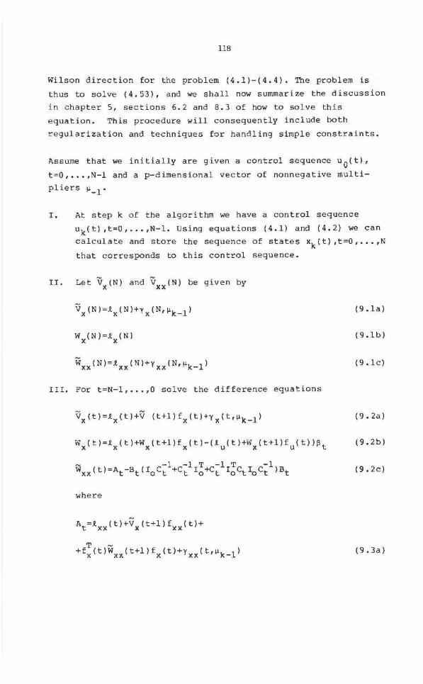
118

Wilson direction for the problem (4.1)-(4.4). The problem is

thus to solve (4.53), and we shall now summarize the discussion

in chapter 5, sections 6.2 and 8.3 of how to solve this

equation. This procedure will consequently include both

regularization and techniques f or handling simple constraints.

Assume that we initially are given a control sequence u 0(t),

t=O, •.• ,N-1 anda p-dimensional vector of nonnegative multi­

pliers µ _1

.

I. At step k of the algorithm we have a control sequence

II.

uk( t) ,t=O, ... ,N- 1. Using equations ( 4 .1) and ( 4. 2) we can

calculate and store the sequence of states xk(t),t=O, ••• ,N

that corresponds to this control sequence.

Let Vx(N) and V (N} be given by XX

W (N)=1 (N) X X

(9.la}

( 9. lb}

(9. le)

III. For t=N-1, .•. ,0 solve the difference equations

(9. 2a)

W ( t ) = 1 ( t ) +W ( t + l } f ( t ) - ( 1 ( t ) +W ( t + l } f ( t ) ) ~ t X X X X U X U

(9.2b)

(9. 2c)

where

{9.3a)

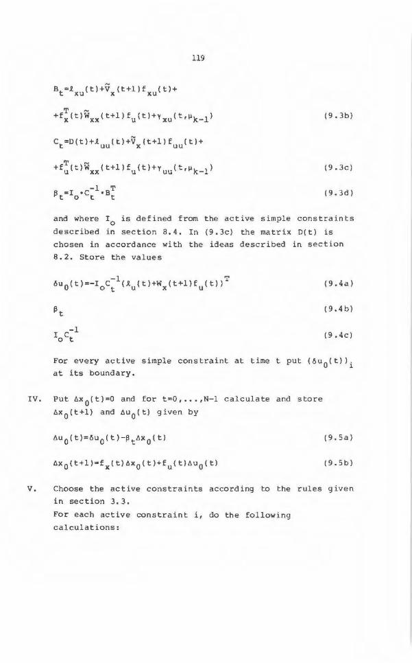
119

(9 . 3b)

(9 . 3c)

-1 T ~ =I • C • B t 0 t t (9 . 3d)

and where !0

is defined from the active simple constraints

described in section 8.4. In (9.3c) th e matrix D(t) is

chosen in accordance with the ideas described in section

8.2. Store the values

öuo(t)=-roc-1 (~ (t)+W (t+l)f (t))T t U X U

(9 . 4a)

~t ( 9. 4 b)

(9 . 4c)

For every active simple constraint at time t put ( ö u0(t))i

at its boundary.

IV . Put t1x0

(t)=O and for t=O, ... ,N-1 calculate and store

t1x0

(t+l) and t1u 0 (t) given by

( 9. Sal

(9 . Sb)

V. Choose the active constraints according to the rules given

in section 3. 3 .

For each active constraint i, do the following

calculations:

Store the values:

t>t. 1

120

For t=ti-1, ••• ,0 so lve the difference equation

Wi(t)=Wi(t+l )(f (t)-f (t)~t) X X X U

with the boundary value

and dur ing these calculations compute and store

(9 .6a)

(9.6b)

(9. 7a)

(9. 7b)

( 9 . 8)

Put 6xi(O) =O and for t=O, ..• ,N-1 calculate 6 xi(t+l) and

6ui(t) from

6u . ( t) = Ö U . ( t ) -~ t [) X ( t . ) 1 1 l

(9.9a)

( 9. 9b)

During these calculations compute and store the element

a . . given by lJ

a .. =hj(t. )6x. (t. )+hj(t. )6u . (t.) l J X ] l J U ] l J

(9 .10)

for every constraint j in the active set.

The elements a . . in (9.10) define the matrix A in (3.9) in l]

section 3.3. The elements of the right hand s i de vector in

(3.10) are calculated as

121

(9.11)

After having solved ( 3 .8) for the current set of active

constraints, put öx(O l=O and solve t he equations

(9 . 12a}

(9 .12b)

Du ring these calculations, calculate the values of öJ zk in

(7.7) and also check if the non-active constraints of

(4.53d} are violated .

If the matrix A becomes sing ular during these calcu­

lations, the assumption A2 given in section 5.2 is

viola ted. Then special mea s ures must be taken (cf

section 6 . 2).

VI . Let öx(t) and öu(t) be the result of the previous step and

µk the value of the Lagrange multipliers for the con­

straints (4 . 53d) obtained at the solution . N-1 2 If E löu(t) I <i:: for some g iven i::>O go to step VIII. t=O

VI I. Let

where o:k is chosen according to the rules given in

section (7.4). Put k=k+l and go back to step I.

VIII. Accept uk(t ) , t=O , ... ,N-1 as the optimal control.

9 . 3 Relationship to other algorithms

( 9 .13)

After describing our algori thm for discrete time optimal control

problems we will now make a comparison with two other proposed

methods in this field, namely the DDP-me thod in Jacobson and

122

Mayne (1 970) and th e new DDP- algor ithm by Ohno (1978). We will

here consider the version of the DDP-method denoted as small

variations in control. Moreover we assume that in Ohno' s method,

the Newton method is used as the local iteration procedure for

finding a solution to the Kuhn - Tucker necessary condi t ion.

These three methods (our method, and the two DDP-methods) all

give an increment of the type

6u(t) = öu(t)-~t·dx(t) (9.14)

but the choices of öu(t), ~tand dx(t) differ for the methods.

We first assume that we have no constraints of the type {4.4).

In both the DDP-methods, the backward equations are solved as in

(9.2) but in the expressions (9.3), the vector V (t) is replaced X

by Wx(t). Hence it is not necessary to solve the difference

equation for Vx{t). The calculation of ~t is made in accordance

with (9.3d) for all t hree methods but again in the expressions

for ~ t and Ct' Vx(t) is e xchanged for Wx{t) for the DDP-methods.

This is also the only difference in the calculation of öu(t).

Another difference appears in the calculation of the value of

dx(t) in (9.14). Our algorithm uses dx(t)=6x(t) where 6 x(t) is

obtained from the solution to (9.5). In both the DDP-methods

dx( t) is calculated as

(9.15)

where xk(t) denotes the states corresponding to the con t rol s

uk(t) and xk+l<tl denotes the states corresponding to the cont­

rols uk+l(t) =uk(t)+6u(t). Hence again our method requires the

solution of an extra set of difference equations in order to get

an exact Newton direction. (If we refrain from using an exact

Newton method we could of course also use (9.1 5)).

To obtain global convergence in our algorithm, we adjust the

v~riable ak in (9.13) so that a sufficient reduction is obtained

in the objective function. In Jacobson and Mayne the new control

seqµence is given in a similar way, namely by

123

where c is chosen so that a decrease is obtained in the objec­

tive function . Ohno's method is only supposed to be applied

close to a solution, so he uses

(9.17)

without any step-size reduction procedure at all (cf Theorem

7. 2) .

As shown above, our method requires the solution of two ex tra

sets of difference equations. But because the variables in these

difference equations are of dimension nx' the extra computer

work for solving these equations is small compared to the solu­

tion of the Riccati equation which is nxxnx. Also these two

extra difference equations are necessary to obtain an exact

Newton direction and hence the reason why we easily prove global

convergence and locally quadratic convergence.

Assume that we have constraints of the type ( 4. 4). Both the DDP­

methods require that these constraints are explicit functions of

the controls . If these methods are used on problems which have

pure state constraints, the state transition equation must be

used once or several times to get a constraint that is an expli­

cit function of u . Both the DDP-methods take care of the con­

straints in the same way as we handle simple constraints in

Section 8 . 2 . In our method, two difference equations are solved

for each active constraint (cf (9.7) and (9.9)) and for each set

of active constraints we have to solve the dif ference equation

(9.12). Hence, again our method has to solve extra difference

equations. On the other hand, our method gives a better es timate

of the active constraints, because in the other methods, the

choice of active constraints is made when solving the Riccati

equation, and this choice cannot be changed during the rest of

the iteration. A result of this fact can be an increased number

of iterations for the DDP-methods.

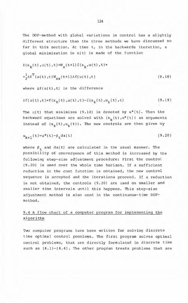
124

The DDP-method with global variations in control has a sl ightl y

different structure than the three methods we have discussed so

far in th is sectio n. At t ime t, in the backwards iteration, a

global minimization in u(t ) i s made of the func tion

i ( X k ( t) / U ( t ) / t ) +W X ( t + 1 ) f ( X k / U ( t) , t ) +

(9 .18)

where 6f(u(t) ,t) i s the diffe rence

6f(u(t) ,t)=f(xk (t) ,u(t) ,t)-f(xk(t} , u k ( t) ,t) (9 .19)

The u(t} that min imizes (9.18) is denoted by u*(t) . Then the

backward equations are solved with (xk(t) ,u*(t)) as arguments

ins t ead of (xk(t),uk(t)). The new controls are then given b y

{9.20)

whe r e ~ t a nd d x( t) a r e calculated in t he usual manne r . The

possibility of convergence of thi s me t hod is increased by t he

f o llowing ste p-size adjustment procedure: First the control

(9.20) i s used over the who le time horizon. If a sufficient

red uct ion in the cost f unction is obtained , t he new control

sequence is accepted and the iterat ions proceed . If a r e duc tion

is not obtained , the controls (9.20) are used on srnaller and

smaller time intervals unti l t hi s happens. This step- size

ad j u s tment method is also used in the continuous-tirne DDP­

method.

9.4 A flow chart of a cornputer p rogram f or implementing the

algori thm

Two compu t er programs have been written for solving discre t e

t ime optima l control problems. The f ir s t p rogram sol ves optimal

control problems, that are directly form ula t ed in discrete tirne

such as (4.1)-(4.4). Th e other program treats prob lems that a re

125

f o rmulated in continuous t i me, wh i le t he control is constrained

to be piecewise constant between sampl ing instants. This prob­

lem, along wi t h r e l evant equations , i s further discussed in the

appendix .

The basic steps in t hese two programs are the same. In fact,

they have the same main program - only certain subroutines

differ between t he two programs.

The organization of the calculations basically fo l low the sum­

mary of the algorithm, given i n the Section 9 . 2 . A flow char t of

the main program has the fo l lowing structure:

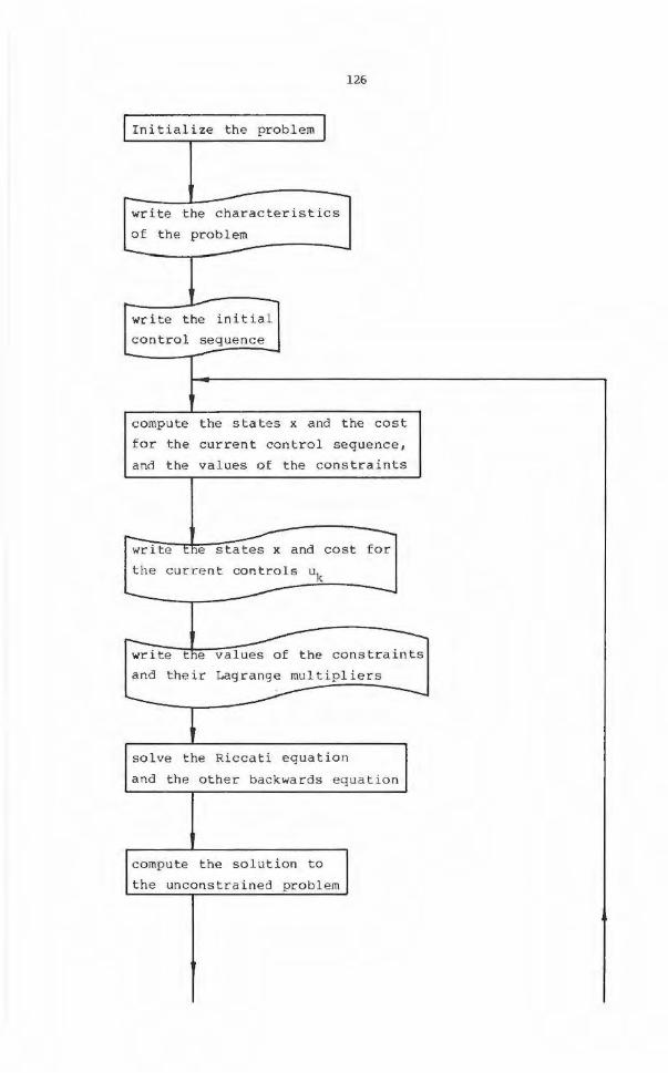
126

I ni tia! ize t he problem I

-write the c harac t eristics

of the prob l em

---~-------~-----~-

r-------wri t e t he initial

con trol sequence

c ompute t he sta t es x and t he cost

fo r the cur rent contro l sequence ,

and the va l ues of the constraints

--­w-r~i~t-e--.t41-,e-s~t~a~tes x and cost f or

the curre nt controls uk

~---"--------~------

----wr~i~t-e--,t~h-,e-v-a-:-1-ues of the constr aints

and t he ir Lagrange multipl ie r s ---s o lve the Riccati equa t ion

a nd the o t her backward s equation

compute the solution to

t he unconstrained pr oblem

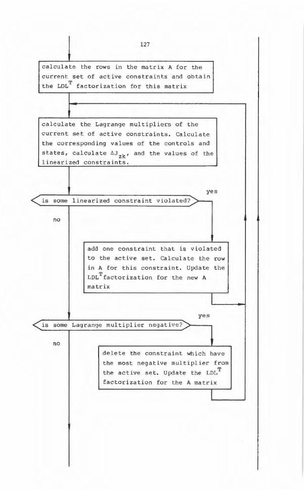
127

calculate the rows in the matrix A for the

current set of active constraints and obtain

the LDLT factorization for this matrix

calc ulate the Lagrange mult i pliers of the

current se t of active constraints . Calculate

the corresponding values of the controls and

states , calculate 6Jzk' and the values of the

l inearized constraints .

~s

is some linearized constraint violated?.:>---

no

add one constraint that is violated

to the active set. Calculate the row

in A for this constraint. Update the

LDLTfactorization for the new A

matrix

yes

is some Lagrange multiplier negative ?

no

delete the constraint which have

the most negative multiplier from

the active set. Update the LDLT

factorization for the A matrix

128

2 N-1 2 calculate \ tiul = l \tiu(t)j

t =O

yes

no

(s top

I 1e t cc=l I

for the control uk+a·ti~ calculate the

states , value of the constraints, the

cost and the values of JP(u) and JL(u )

no

is the Watchdog crite rion sat isfied?..........->-~~--'

yes

write values of ukl

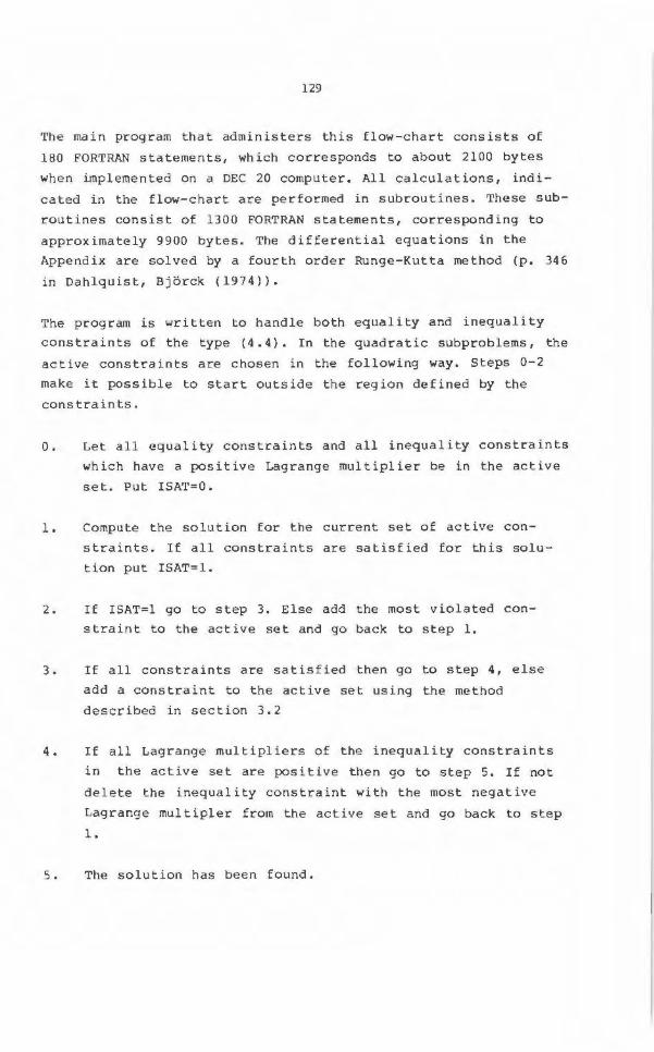
129

The main program that administers this flow-chart consists of

180 FORTRAN statements, which corresponds to about 2100 bytes

when implemented on a DEC 20 computer . All calculations, ind i­

cated in the flow-chart are performed in subroutines . These sub­

routines consist of 1300 FORTRAN statements, corresponding to

approximately 9900 bytes . The differen t ial equations in the

Appendix are solved by a fourth order Runge-Kutta method (p . 346

in Dahlquist, Björck ( 1974)).

The program is written to handle both equality and inequality

constraints of the type (4 . 4) . In the quadratic subproblems, the

active constraints are chosen in the following way . Steps 0-2

make it possible to start outside the region defined by the

constraints .

o. Let all equality constraints and all inequality constraints

which have a positive Lagrange multiplier be in th e active

set . Put ISAT=O.

1 . Compute the solution for the current set of active con­

straints . If all constraints are satisfied for this solu­

tion put ISAT=l.

2. If ISAT=l go to step 3 . Else add t he most violated con­

straint to the active set and go back to step 1.

3 . If all constraints are satisfied then go to step 4 , else

add a constraint to the active set using the method

described in section 3.2

4. If all Lagrange multipliers of the inequality constraints

in the active set are positive then go to step 5 . If not

delete the inequality constraint with the most negative

Lagrange multiple r f rom the active set and go back to step

1.

5. The solution has been found .

130

The idea is to add viola t ed inequality constrain t s to the active

set until all constraint s are satisf ied. Then we can use the a l­

gori thm in Section 3.2 (steps 3- 5).

9.5 User-program i n terface.

The organization of the program is such t hat t he user specifies

his non-linear optima l con t rol problem in a separate FORTRAN

subroutine. This FORTRAN subroutine communicates with the main

program through four named COMMON blocks . I n these COMMON blocks

the following information should be given:

n x' the number of s t ates

n u' the number of controls

N, the number of sampl ing instants

p, the number of inequality cons traints.

µ I the values of the penalty parameters in t he Watchdog

technique (7. 3).

e, Parameter to determine the termination criterion.

Moreover the values of the time instants, t 1 , ..• , tp at which

the constraints are given must be specified , as well as lower

a nd upper bou nds on the contro l signals.

Al so, for given x and u the state transition function f (see

(4.1)) as wel l as its first and second order derivatives should

be calculated. Similar l y , for given x and u the criterion func­

tion ~ along with its fi r st and second der i vatives with respect

to x ana u should a lso be specified as well as the constraint . i

funct 1ons h together with their first and second order deriva-

tives with resepct to x and u. Finally, the initial values for

tb e control-signals and for the Lagrange mult ipliers must be

specified.

A typical subroutine is depicted in Figure 9.1

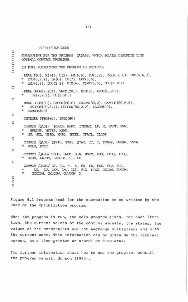
131

SUBROUI'INE USER c C SUBROUI'INE FOR THE PRCX>RAM QADAPP, WHICA OOLVES DISCRETE TIME C OPI'IMAL CCNTROL PROBLEMS . c C IN THIS SUBROUTINE THE PROBLEM IS DEFINED . c

c

c

c

c

c

c

c

c c c

REAL F(6), X(74), U(2), FX(6,6), FU(6,2), FXX(6,6,6) , FXU(6,6,2), * FUU(6,2,2), LX(6), lll(2), LXX(6,6), * LXU(6,2), UJU(2,2), FIX(6), FIXX(6,6), U.10(2 ,201)

REAL UNOM(2, 201). VNCt-1(201), XIN(6). XNCM(6, 201). * UL(2,201), UU(2,201)

REAL GCOO ( 80 ), GXC'CTN ( 80 , 6 ) , GUCOO ( 80, 2 ). GXXCCN ( 80, 6 , 6 ). * GXUCCN(80,6,2), GUUCDN(80,2,2), 1ACON(80 ), * Il\MBDA. ( 80)

INTEGER ITEQ ( 80). IPElO ( 80)

COvlMON /QADl / IGAAD, KOOT, ITEMJ\X, LP, N, NACT, NE.W, * NPR.lNI', NSTEP, NEND, * NU, NEQ, NIEX), NAEQ, INDEL, IFAIL, II.roP

C<M1CN /QAD2/ EPSIL, ETAl, ETA2, IT, T, TSAMP, UNORM, \/NEW, * VOLD, PCIC

CCMMCN /QAD3/ UNQvl, VNQvl, XIN, XNQvl, UJO, ITEX), TPEQ, * GCON, IACCN, LAMBDA, UL, UU

C<M1CN /OAD4/ SF, SL, F, U, FX, FU, FXX, FXU, FUU, * LX, UJ, LXX, LXU , llJU, FIX, FIXX, GXC'CTN, GUCOO, * GXXC'ON, GXUCCN, GUUCON, X

Figure 9 . 1 Program head for the subroutine to be written by the

user of the optimization program .

When the program is run, the main program gives , for each itera­

tion, the current values of the control signals, the states, the

values of the constraints and the Lagrange multipliers and also

the current cost. This information can be given on the terminal

screen, on a line -printer or stored on disc-are a .

For further information about how to use the program, consul t

the program manual, Jenson {1983) .

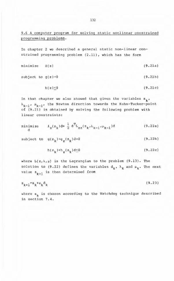
132

9.6 A computer prog ram for solving s tatic nonlinear constrained

p rogramming problems.

In chapter 2 we described a general static non-linear con­

strained programming problem ( 2 .11), which has the form

minimize .l ( z) (9.2la)

subject to g(z)=O (9.2lb)

h(Z)2_0 (9 . 2lc)

In that chapter we also showed that given the variables zk,

Ak-l ' µk-l' the Newton direc tion towards the Kuhn - Tucker-point

of (9.21 ) is obtained by solving the following problem with

linear constraints:

mi n i mize d

subject to

(9.22a)

(9.22b)

( 9. 22c)

where L(z,A,µ) is the Lagrangian to the problem (9.13). The

solution to (9.22) def ines the variables dk' Ak and µk . The next

value zk+l is then determined from

(9 . 23)

where ak is chosen according to the Watchdog technique described

in section 7.4.

133

A computer program has been developed for the problem (9.21)

using the i tera t ions (9 . 23). Similarly to the program for opti­

mal control problems, a subroutine has to be written by the

user. This subroutine should specify the following values:

n, the number of variables

m1 , t he numbe r of equality constraints

m2

, the number of inequality constraints.

Also for any given value of z, the values of the functions

J.( z ), g(z), and h (z) (defined in (9 . 21)) along with their first

and second order derivatives with respect to z have to be

g i ven.

When t he program is run the values of zk' g(zk) , h(z k ) ' Ak and

µk are printed on a file for each iteration.

In the program the quadratic sub- problems (9.22) are solved

using the technique described in sec tion 3 . 3. The NAG-routines

FOIBRF and F04AXF are used for factoriz ing the system matrix in

(3 . 6) and (3.7) a nd for solving this system of linear equa ­

tions.

134

135

10. AN OPTIMAL POWER DISTRIBUTION PROBLEM

10.1 Introduction

In this chapter we consider an e l ectrical network of the same

kind as that of example 2 . 1 . It will however be of more realis t ic

complexity. We assume that the network has a number of nodes .

Some of the nodes are connected by elec trica l lines . Not all

nodes need to have direct lines between each other , but all nodes

are connected. At each node there are power generators , power

consumers or both . A node can have more than one generator . Each

generator is allowed to produce power within a given interval

on l y. The consumers requ ire a known amount of electric power . On

some of the lines there may also be transformers . To each ge ne ­

rator there is assigned a cost function, whose value is de ter­

mined by the amount of power generated .

The problem is now to adjust the generated power so that the

total cost, summed over each power generator , is mi nimized when

the power demand from the cons umers i s sat i sf i ed .

This problem is of the type {2 . 11 ). More specifically, we may

define the problem as follows:

Let the vec t or z consist of all values that de s c ribe the network

with t he following quantitites:

Vi the voltage amplitude at each node

~i the phase angle of each node (except the slack- node} .

t. the amplitude ratio for transformer j J

PGk th e r eal power produced by ge nerator k

QG~ the complex power produced by generator~.

136

Objective function

We assume t hat only the real power generators have associated

costs. Hence our cost function is

(10.1)

The index k on ek impl ies that the cost functions may be diffe­

rent for the different generators.

Equality constraints

Each node must be in balance, both with respect to real and to

complex power. This gives us the constraints for each node. As in

example 2.1 we get t hat for node l these constraints are" (see

( 2. 2))

(10.2a)

Inequality constraints

I n order to operate safely, the lines must not be overloaded.

Tha t is to eac h line there is an upper limit on the heat produced

i n the line. (cf equation (2.7)}.

Also, the network must be stable . Therefore the phase angle

between two nodes a t each end of a line must not differ by more n

tha n 2 . ror one of the nodes the phase angle is fixed to zero.

This node is usually called the slack node.

Simple constraints

The generators have limited capaci ty. Therefore for each gene ­

rator, the generated power must be within a given interval.

137

(10.3a)

(10 . 3b )

10.2 The test e xample

We choose an e xample given in Arriatti (1971 ), which is often

used as a t est example for algorithms designed to solve elelctri ­

cal power distribution problems. It consists of 10 nodes and 13

transmission lines. In 5 of these lines there is a transformer .

The total number of power generators is 14, allocated at 7 diffe­

rent nodes. At each of these 7 nodes there is also a reactive

generator . This gives a total of 45 free variables, 20 equality

constraints, 20 inequality constraints and 41 simple constraints.

The varibles are: 10 voltage amplitudes, 2 phase angles, S trans­

formers, 7 reactive power generators and 14 real power genera ­

tors . The 22 inequality constraints consist of 13 from maximum

capacity at the 13 lines and 8 f rom phase angle differences . The

41 simple constraints are : 10 for the voltage amplitudes , 6 phase

angles directly connected to the slack node, 5 transformers , 14

real power generators and 7 reactive generators . The geometry of

the network is given by figure 10.1.

This problem is an exampl e of a so-called sparse prob l em . Spar­

sity here means that the Hessian of the objective function and

the constraints, and the Jacobian of the constraints contain many

zeros.

The figures 10.2a and 10.2b show non-zero elements in the Hessian

of the Lagrangian of the problem (equations (10 .l) and (10.2))

and in the Jacobian of the equality constrain ts (equat i on

(10.2ab)) and inequality constraints (equation (2.7)). The vari­

ables are ordered in the following way:

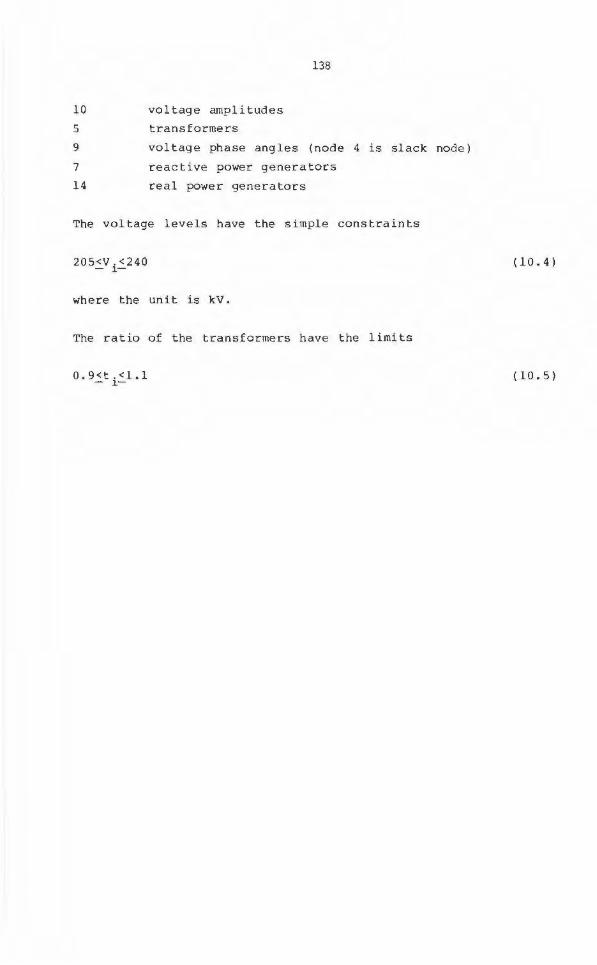
10

5

9

7

14

vol tage ampli tudes

transformers

138

voltage phase angles (node 4 i s slack node)

reactive power generators

real power generators

The voltage levels have the simple constraints

205<V.<240 - 1-

where the unit is kV .

The ratio of the t rans formers have the limits

0.9<t .<l.l - 1-

(10.4)

(10.5)

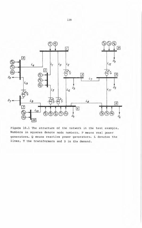
139

0

0 o~

L~ LI LJ Lz L1z

0 'i 7f [l] @] o.,

L7

LIJ

L5 D L' :3 L11

05

07 l, L8 @] [11 l±J L10

04 [@

~

Figure 10 . l The structure of the network in the test example .

Numbers in squares deno t e node numbers. P means real power

generators. Q means reactive powe r generators. L denotes the

lines , T th e transformers and D is the demand .

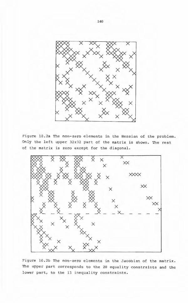
140

Figure 10 . 2a The non-zero elements in the Hessian of the problem.

Only the left upper 32x32 part of the matrix is shown . The rest

of the matrix is zero except for the diagonal.

X

X X

X

X

X X

- x_

xxxx

XX

XX XX

Figure 10 . 2b The non- zero elements in the Jacobian of the matrix .

The upper part corresponds to the 20 equality constraints and the

lower part, to the 13 inequality constraints.

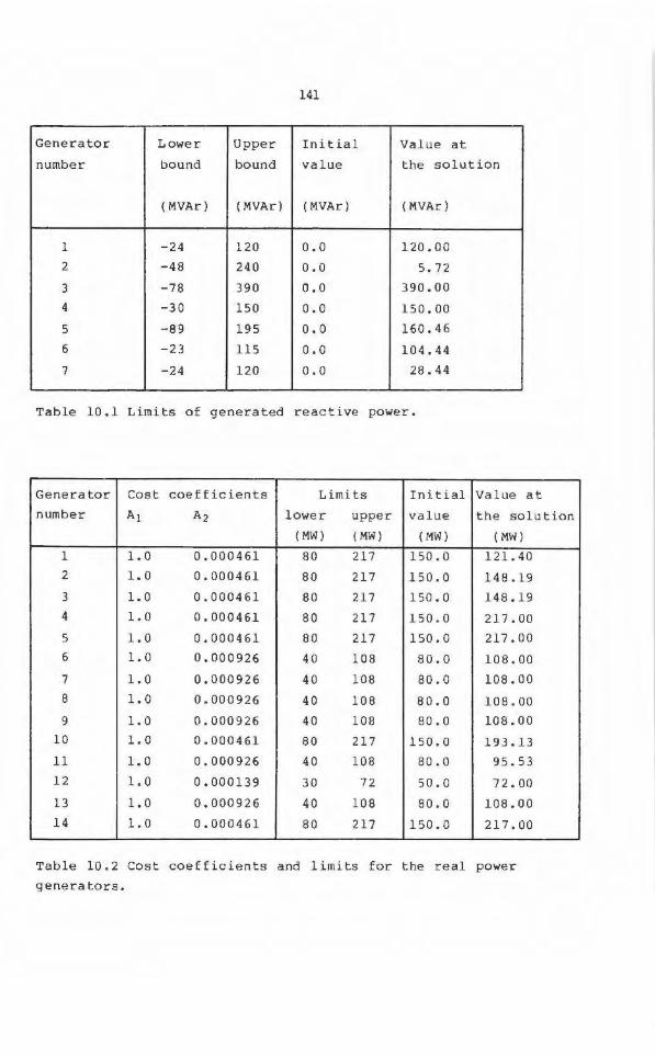
141

Generator Lower Upper Initial Value at

number bound bound value the solution

(MVAr) (MVAr) (MVAr) (MVAr)

1 -24 120 0 . 0 120 . 00

2 -48 240 0 . 0 5. 72

3 -78 390 o.o 390.00

4 -30 150 0.0 150.00

5 - 89 195 o.o 160.46

6 -23 115 o. o 104.44

7 -24 120 o.o 28. 44

Table 10 . l Limits of generated reactive power .

Generator Cost coeff icients Limits Initial Value a t

number A1 A2 lower upper val ue the solution

(MW) (MW) (MW) (MW)

l l. 0 0.000461 80 217 150 . 0 121. 40

2 l. 0 0.000461 80 217 150 .0 148.19

3 l. 0 0 . 000461 80 217 150.0 148.19

4 l. 0 0 . 000461 80 217 150 . 0 217.00

5 l. 0 0 . 000461 80 217 150 .0 217.00

6 l. 0 0.000926 40 108 80.0 108 . 00

7 l. 0 0.000926 40 108 80 . 0 108. 00

8 l. 0 0 . 000926 40 108 80.0 108 . 00

9 l. 0 0 . 000926 40 108 80.0 108.00

10 l. 0 0 . 000461 80 217 150.0 193.13

11 l. 0 0 . 000926 40 108 80 . 0 95.5 3

12 l. 0 0. 000139 30 72 50.0 72. 00

13 1.0 0.000926 40 108 80 . 0 108 . 00

14 l. 0 0.000461 80 217 150 . 0 217.00

Table 10.2 Cost coefficients and limits for the real power

generators.

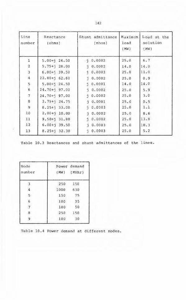
142

Line Reactance Shunt admittance Maximum Load a t the

number {ohms) (mhos) load solution

( MW) (MW)

1 5.00+j 24. 50 j 0.0002 25.0 6.7

2 5 . 75+j 28 . 00 j 0.0002 1 4.0 14.0

3 6 . OO+j 39.50 j 0 . 0003 25 .0 11. 0

4 22 . BO+j 62 . 60 j 0 . 000 2 25.0 0.9

5 5 . 00+j 24 . 50 j 0 . 0001 14 . 0 14.0

6 2 4 . 70+j 97. 0 0 j 0 . 0002 25 . 0 5.9

7 24. 70 +j 97.00 j 0 . 0002 25 .0 3.0

8 3 . 75+j 24.7 5 j 0.0001 25.0 0. 5

9 8. 25+j 33. 00 j 0.0003 25.0 1.1

10 2 . 00+j 10 . 00 j 0 . 0002 25.0 8 .6

11 9 . 50+j 31 .80 j 0.0002 25 . 0 13 . 8

12 6 . 00+j 39.50 j 0 . 0003 2 5 .0 10.3

13 8 . 25+j 32 . 30 j 0.0003 25 . 0 5.2

Table 10.3 Reactances and shunt admittq nces of the lines .

Node Power demand

number (MW) (MVAr)

3 250 150

4 1000 630

5 150 75

6 100 35

7 100 50

8 250 150

9 100 30

Table 10 . 4 Power demand at different nodes .

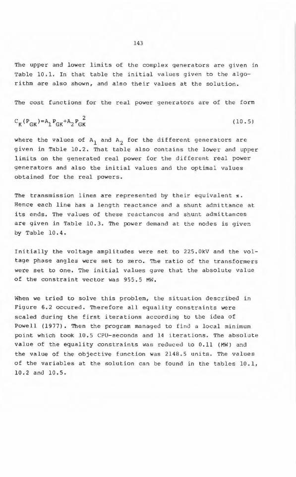
143

The upper and lower l imit s of t he complex generators are given in

Tab le 10 . 1 . In that table the initial values given to the algo­

rithm are also shown, and also their values at the solution .

The cost functions for the real power generators are of the form

(10. 5)

where the values of A1 and A2 for the dif feren t generators are

g iven in Table 10.2 . Th a t table also con t ains the lower and upper

limits on the generated real power for the different r eal power

generators ana also the initial values and the optimal values

o b tained for the real powers.

The transmission lines are represented by their equivalent n .

Hence each line has a leng t h r eac tance and a shunt admit t ance at

i t s ends . The va l ues of these reac t ance s and shunt admittances

are given in Table 10 . 3 . The power demand at the nodes is given

by Table 10 . 4 .

Initia l ly the voltage amplitudes were set to 225.0kV and the vol­

tage phase angles were set to zero. The r atio of the trans formers

were set to one . The initial values gave that the absolute value

of the constraint vector was 955.5 MW.

When we tried to solve this p roblem, the si tuation described in

Figure 6.2 occured . Therefore all equality constraints were

scal ed during the first iterations according to the idea of

Powell (1977). Then the program managed to find a local minimum

point which took 10.5 CPU-seconds ana 14 iterations . The absolute

value of the equality constraints wa s reduced to 0 . 11 (MW) and

the value of the ob jec tive function was 2148 . 5 un its . The values

of the variables at the solution can be found in the tabl es 10 . l,

10. 2 and 10 . 5 .

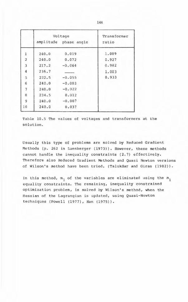
144

Voltage Transformer

ampli tude phase angle ratio

l 240.0 0 .019 1. 089

2 240.0 0.072 0.927

3 217 . 2 - 0 . 064 0 . 982

4 236.7 -- l. 003 5 222.S -0.055 0. 9 33

6 240.0 -0 . 003

7 240.0 -0.022

8 234 . 5 0 . 012

9 240.0 -0 .007

10 240 . 0 0.037

Table 10 . 5 The values of voltages a nd transformers at the

solution.

Usually this type of problems are solved by Reduced Gradient

Methods (p. 262 in Luenberger (1973)). However , these methods

cannot handle the inequality constraints ( 2 .7) effec tive ly.

Therefore also Reduced Gradient Methods and Quasi Newton versions

o f Wi l s o n ' s method have been tried. (Talukda r and Giras (1982)).

In this method , m1

of the var i ables a r e eliminated using the m1

equality constraints . The remaining , inequali ty constrained

optimization problem , is sol ved by Wilson ' s method , when the

Hessian of the Lagrangian is u pda ted, using Quasi-Newton

t echniques (Powell (1977), Han (1975)).

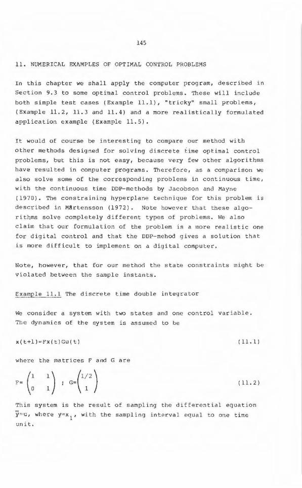
145

11. NUMERI CAL EXAMPLES OF OPTIMAL CONTROL PROBLEMS

In this chapter we shall apply the computer program , described in

Section 9 . 3 to some optimal control problems . These will i nclude

both simple test cases ( Example 11 . 1), "tr icky" small probl ems,

(Example 11.2, 11. 3 and 11.4) and a more realistically formulated

a p p lication example (Example 11 .5).

It would of course be interesting to compare our method with

other methods designed for solving discrete time optimal control

problems , but this is not easy , because very few othe r algori thms

hav e resul t ed in computer programs . Therefore , as a c omparison we

also solve some of the corresponding problems in continuous time ,

with the continuous time DDP- methods by Jacobson and Mayne

(1970) . The constraining hyperplane technigue for this problem is

described in M!rtensson (1972). Note however that t hese algo­

r ithms s o lve completely different types af problems . We a l so

cla i m that our formula t ion af the problem is a more r ealistic one

f or dig i tal control and that the DDP- mehod gives a solution that

is more difficult ta implement an a digital computer .

Note, however, that for our method the state co ns traints might be

violated betwee n the sample i ns t ants .

Example 11.l The discrete time double integrator

We consider a s ystem with two states and one control variab l e .

The dy nam i cs af t he s ystem is assumed ta be

x(t+l) = Fx(t)Gu(t) ( 11. l)

where the matrices P and G are

( 11. 2)

This s ystem is the result af sampling the differential equat ion

y=u , where y=x1

, with the sampling interval equal ta on e time

un it.

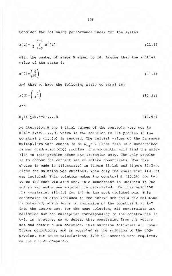
146

Consider the following performance index fo r the system

1 N-1 2 J{u):: i:: u (t) 2 t =O

{ 11. 3)

with the number of steps N equal to 10. Assume tha t the initial

va lue o f the s t ate is

{ 11. 4)

and that we have the following state constraints:

(11.Sa)

and

X l ( t ).::_10 ,t=O , ..• , N (11.Sb)

At iteration 0 the initial values of the controls were set to

u(t) =-2 ,t=0, •.• ,9, which is the sol ution to t he problem if the

cons tra i nt (11 . Sb ) is removed . The init ial values of the Lagrange

multiplier s were chose n to be µ _1

=0. Since this is a cons trained

linear quad r atic (CLQ) p r oblem , the algorithm will find the solu­

tion to this problem after one iteration only . The only problem

is to choose t he correc t set of active const raints . How this

choice is made is ill ustrated in Figure 11.lab a nd Figure ll .2ab.

First the solution was ob t ained , when only t he constraint (10.Sa )

was included . This solution makes the constraint (10 . Sb) for t=S

to be the mast v iola t ed one. This constraint is included in the

active set a nd a ne w so lu tion is calculated. For t h is solution

the constraint (11.Sb) for t=3 is the mast violated one. This

constraint i s also inc l uded in the active set and a new solution

is obtained, which leads to inclusion of the constraint at t=7

inta the act i ve set. For the next solution , all constraints are

sa t isfied but the mul t iplier corresponding to the constr aints at

t=S, is negative , so we delete t hat constraint from the active

set and obtain a new solu tion. This solution satisfies all Kuhn­

Tucker conditions, and is accepted as the solution to the CLQ­

probl em . For these calculations, 1 . 09 CPU- s econds were required,

on the DEC - 20 computer .

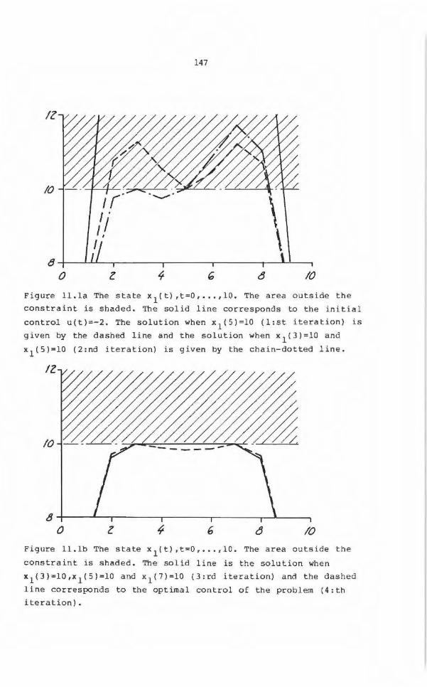
147

\ \

8-1--~-'-.Ll...~~~~~~~~~~~~~~~~--"--'-~-

o Figure 11.la The state x 1 (t) ,t=0, . .. ,10. The area outside the

constraint is shaded. The solid line corresponds to the initial

control u(t)=-2 . The solution when x1

(5)=10 (l:st iteration) is

given by the dashed line and the solution when x1

(3)=10 and

x1

(5)=10 {2:nd iteration) is given by the chain-dotted line.

Il

8~~~~---..-~~~--.~~~~..--~~~~-L-~~~

0 6

Figure 11.lb The state x1(t) ,t=0 , ... ,10 . The area outside the

constraint is shaded. The solid line is the solution when

x 1 (3)=10,x 1 (5)=10 and x 1 (7)=10 (3:rd iteration) and the dashed

line corresponds to the optimal control of the problem (4:th

iteration).

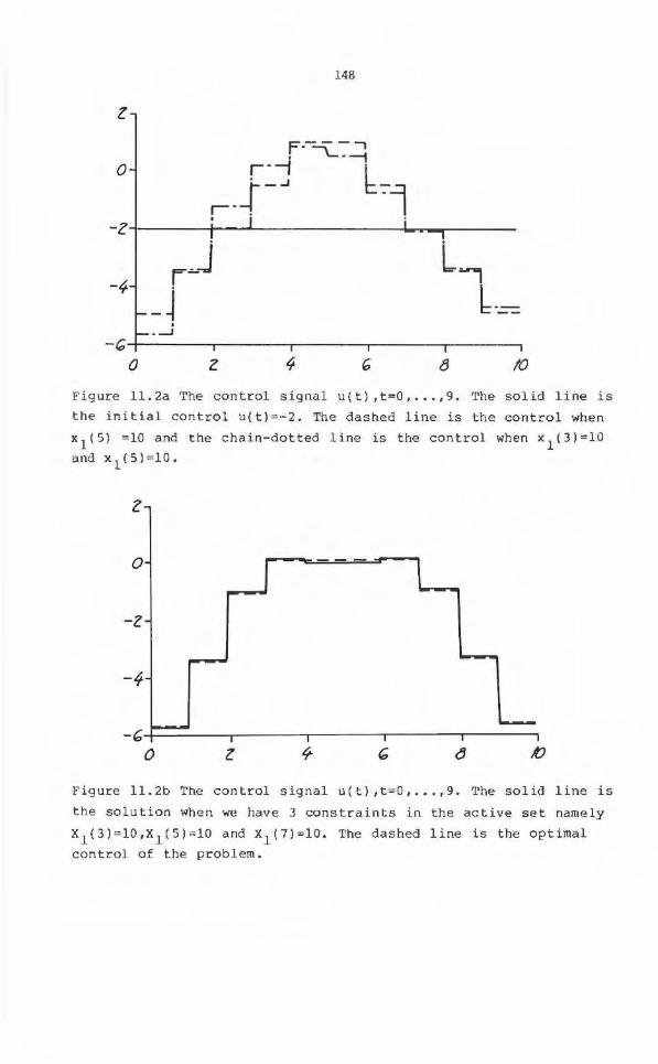
148

Figure ll.2a The control signal u(t) ,t=0, ••• , 9. The solid line i s

the initial control u(t)=-2. The dashed line is the control when

x 1 (S) =10 and the chain-dotted line is the control when x1

(3)=10 and x 1 ( 5) =10.

z

0

-z

-4

-b-+--~~~~~~~~~~~---r~~~--r~~~-.

0 10

Figure ll.2b The control signal u(t) ,t=0, ••. ,9 . The solid line is

the solution when we have 3 constraints in the active set namely

x1 (3)=10,X 1 (5)=10 and x1 (7)=10. The dashed line is the optimal

control of the problem.

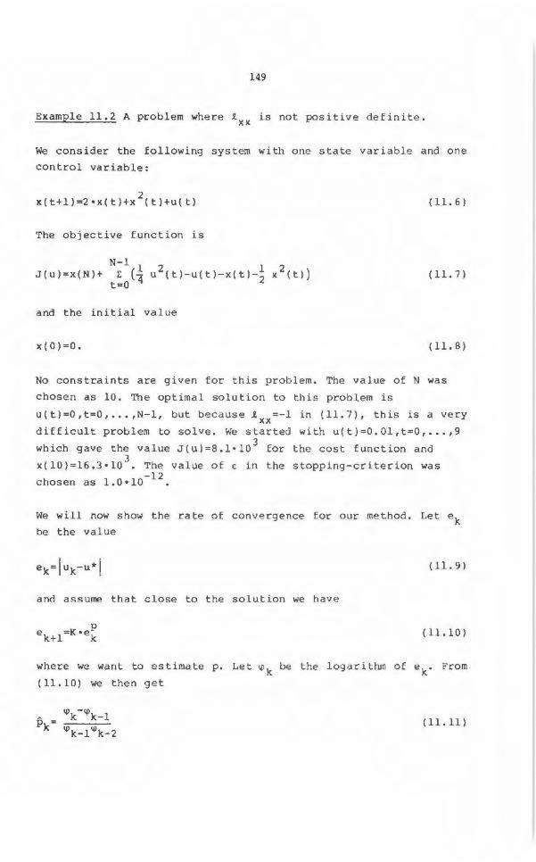
149

Example 11 . 2 A problem where lxx is not positive definite.

We consider the following system with one state variable and one

control variable:

2 x(t+l)=2•x(t)+x (t)+u(t)

The objective function is

N-1 J(u)=x(N)+ E (~ 2 (t) (t) (t) 1 x 2 (tl) t=O 4 u -u -x -2

and the initial value

x(O)=O .

(11.6)

(11. 7)

(11.8)

No constraints are given for this problem . The value of N was

chosen as 10 . Th e optimal solution to this problem is

u(t)=O , t=O, •.• ,N-1 , but because ixx=-1 in (11.7) , this isa very

difficult problem to solve. We started with u(t)=0.01 , t=0, . . . ,9

which gave the value J(u)=8 . l•l03

for the cost function and 3

x(l0) =16 . 3•10 . The value of E in the stopping-cri t erion was

chosen as l.O•l0- 12 .

We will now show the rate of convergence for our method. Le t ek

be the value

( 11. 9)

ancl assume that close to the solution we have

(11.10)

where we want to estimate p. Let lj)k be the logarithm of ek . From

(11 . 10) we then get

(11.11)

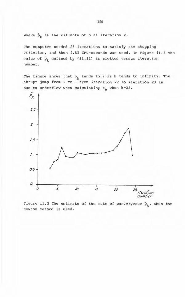
150

where pk is the estimate of p at iteration k.

The computer needed 23 iterations to satisfy the stopping

criterion, and then 2.83 CPU-seconds was used. In Figure 11. 3 the

value of pk defined by (11.11) is plotted versus iteration

number .

The figure shows that pk tends to 2 as k tends to infinity . The

abrupt jump from 2 to 1 from iteration 22 to iteration 23 is

due to underflow when calculating ek when k =23. ,....

.P*

l.5

l.

1.5

I.

0.5

0. 0 10 15 zo

Z5

lferolioo nvmoer

Figure 11 . 3 The estimate of the rate of convergence pk, when the

Newton method is used .

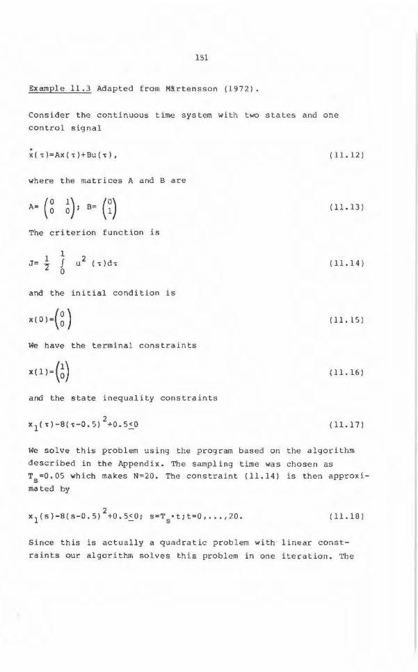
151

Example 11.3 Adapted from M8rtensson (1972) .

Consider the continuous time system with two states and one

control signal

. X{~)=Ax(~)+Bu{~),

where the matrices A and B are

The criterion function is

J= 1 ~

1 f 0

and the initial cond it ion is

X { 0) =( ~ ) We have the terminal constraints

x{l)=(~) and the state inequality constraints

(11.12)

(11.13)

(11.14)

(11.15)

(11.16)

(11.17)

We solve this problem using the program based on the algorithm

described in the Appendix. The sampling time was chosen as

T5

=0.05 which makes N=20. The constraint (11 . 14) is then approxi­

mated by

2 x 1 (s) - 8{s-0 . 5) +0 . 5~0; s=T

5•t;t=0, ..• ,20. (11.18)

Since this is actually a quadratic problem with linear const­

raints our algorithm solves this problem in one iteration. The

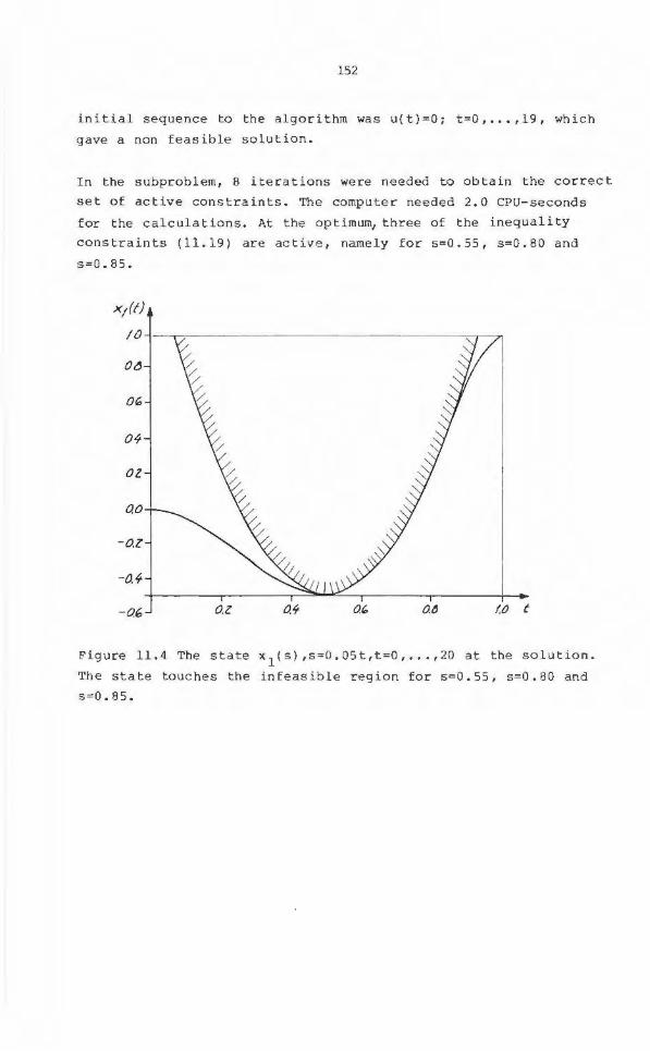
152

initial sequence to the algorithm wa s u(t}=O; t =0 , .• • , 19 , which

gave a non feasible solution.

In t he subproblem, 8 itera t ions we re needed to obtain the correct

set of active constraints. The computer need e d 2.0 CPU-se cond s

for the calculations. At the o p timum, three of the inequality

cons train ts (11.19) are act i ve , name ly for s=0.55 , s=0 .80 a nd

s=0.85.

x1 (t)

10~-~~~~~~~~~~~~~~~~~~~~~~

o" OG

04

oz

0.0

-o.z

-0. 4

-o~ O.l 0.4 10 t

Figure 1 1 . 4 The sta t e x 1 (s),s=0 .05t,t=0, ••. ,20 at t he solution.

The state touches t he infeasible region for s=0.55, s=0.80 and

s=0.85.

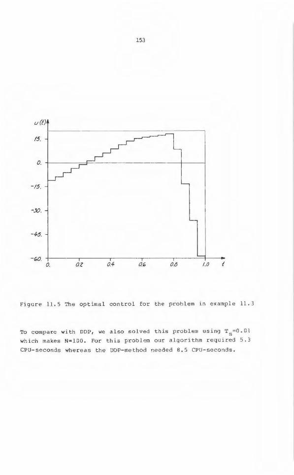
153

v (t)

15.

0.

-15.

-.x?.

-<--5.

-r;,o. 0. oz O.tJ 1.0 t

Figure 11 . 5 The optimal control for the problem in example 11 . 3

To compare with DOP , we also solved t his p r oblem using T5

=0 . 0l

which makes N=lOO . For this problem our algorithm requi r ed 5.3

CPU-seconds whereas the DDP- method needed 8 . 5 CPU-seconds.

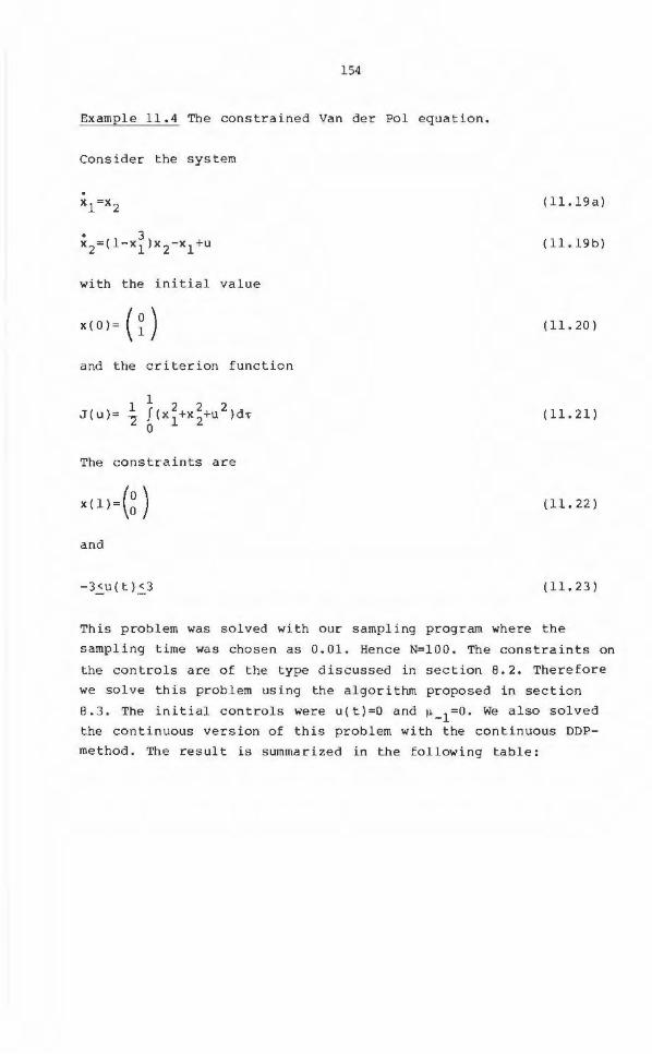
154

Example 11 .4 The constrained Van der Pol equa t ion.

Consider the system

( ll.19a)

(ll.19b)

with the initial value

x(O) =( ~ ) (11.20)

a nd t he cri t erion function

(11.21)

The cons t raints are

x( l)= (~ ) (11.22)

and

-3_:u( t) 2_3 (11.23)

This problem was solved with our sampling program where t he

sampling time was cho sen as 0.01 . Henc e N=lOO . The constraints on

the controls are of the type d i scussed i n section 8 .2. Therefore

we solve t hi s problem using the algorithm proposed i n section

8 . 3. The initial controls were u ( t) =O and µ_1

=0. We a l so sol ved

the continuous version o f this problem with t he continuous DDP­

method. The r esult i s summarized in the following t able :

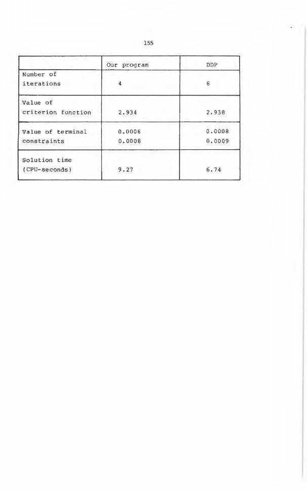
155

Our program DOP

Number of

iterations 4 6

Value of

criterion function 2 .934 2.938

Value of terminal 0.0006 0 .0008

constraints 0.0008 0.0009

Solution time

(CPU-seconds) 9 . 27 6 . 74

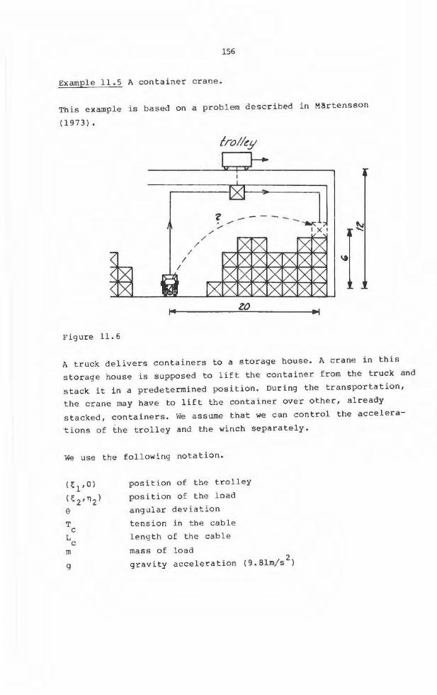
156

Example 11.5 A container crane.

This example is based on a problem described in M8rtensson

(1973).

trolley

zo

Figure 11. 6

A truck delivers containers to a storage house. A crane in thi s

storage house is supposed to lift the container from the truck and

stack it in a predetermined position. During the transportation,

the crane may have to lift the container over other, already

stacked, containers. We assume that we can control the accelera­

tions o f ~he trolley and the winch separately.

We use t he following notation.

(~1 , 0)

(i; 2 I T)2)

e T

c L

c m

g

position of the trolley

position of the load

angular dev ia t ion

t e ns ion in the cable

length o f the cable

mass of load

gravity acceleration (9.8lm/s2

)

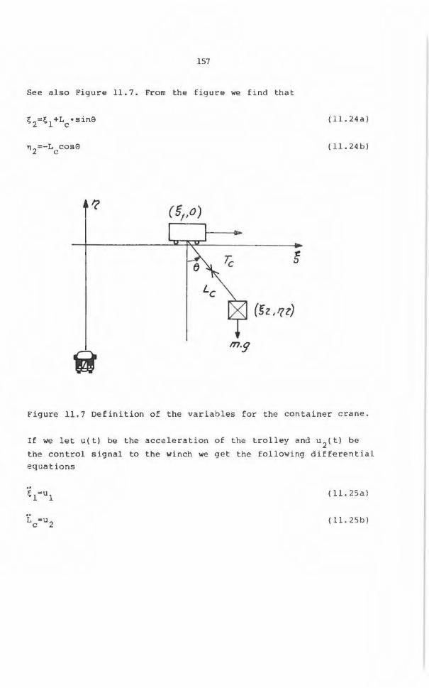
157

See also Figure 11 .7. From the figure we find that

n =-L cose 2 c

m.9

(sz ,qz)

(ll.24a)

(ll.24 b)

Figure 11.7 Definition of the variables fo r the container crane .

If we let u(t) be the acceleration of the trolley and u2(t) be

the control signal to the winch we get the fo llowing differential

equations

'i. =u c 2

(ll.25a)

( 11. 25b)

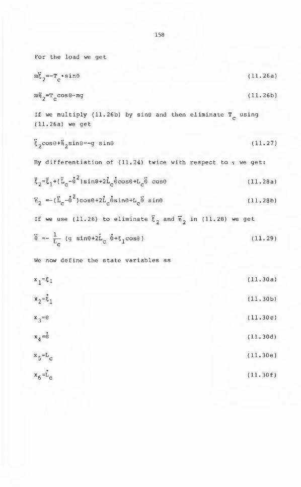
Por the l o ad we ge t

m~ =-T •sin0 2 c

158

( 11. 26a)

(ll.26b)

I f we mul tiply (ll .26b) by sin0 and t hen eliminate T using c

( 11. 26a) we get

(11.27)

By d i fferent iation of (11.24) twice with respect to ~ we get :

•. • 2 • • •. ~2 =- (Lc-0 )cos0+2Lc0sin0+Lc0 sin0

If we use ..

(11.26) to eliminate ~ 2 and T)2

in

1 (g sin0+2Lc 0+~ 1 cos0) Le

We now define the state variables as

X =L s c

. X =L

6 c

(l l. 28a)

( 11. 28b)

(11. 28) we get

(11.29)

( ll.30a)

( 11. 30b)

( ll.30cl

(11. 30d)

(ll.30e)

(l l.30f )

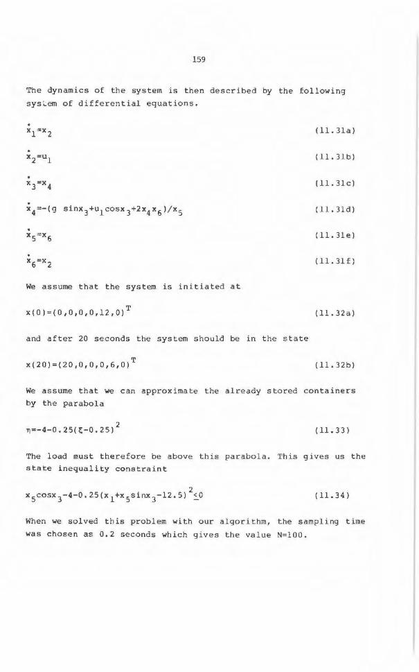
159

The dynamics of the system is then described by the following

sysLem of differential equations .

(ll.3la)

(ll.3lb)

( 11. 3lc)

. x4 =-(g sinx 3+u1 cosx

3+2x4 x

6)/x

5 (ll.3ld)

(ll.3le)

(ll. 3lf)

We assume that the system is initiated at

T x(0)=(0,0,0,0,12,0) {ll . 32a)

and after 20 seconds t he sys t em should be in the state

T x( 20)=(2 0,0,0,0,6,0) {l l . 32b)

We assume that we can approximate the already stored containers

by the parabola

2 n =-4- 0 . 25(~-0.25) (11.33)

The load must therefore be above this parabola . This gives us the

s tate inequal ity constra i nt

(11.34)

When we sol ved th is problem wi th our algor i thm, the sampling t ime

was chose n as 0 . 2 seconds which g i ves the value N=lOO .

160

'l'he in i tial sequence was chosen as

u(·r}=(-~ : ~4) O<-t<lO ( ll.30a)

( -0. 2) u(-t)= 0 .0 3 10<-t< 20 (ll.30b)

which makes a trajectory tha t satisfies only the f irst two of the

t e r minal constra ints ( ll . 32b) .

The iterations were term i na tea when the value of jå ul was smaller than 0.1 . The algorithm needed 3 iterations to find the solu t i o n

and took approxima t ely 55 CPU-seconds .

The posi t ion of the load i s plotted versus time in Figures 11.8

both for the initial control seqence ( Figure 11.Ba) a nd the

o p timal con t rol sequence (Figure 11.Bb).

We a lso solved this probl em in its continuous time counterpar t

using the DDP- method , Jacobson and Mayne (1 970), in combination

with a constr aining hyperplane technique to handle the s tate

constrai nts (1 1.29) as i n Mår t ensson (1973). Also in t his case

the time i nterval [0,20] was divided into 100 steps. The DDP­

p rogram needed 14 iterations and 103 CPU-seconas to solve this

p roblem. The value of the criterion function was in this case

0. 6119 whereas our a lgori thm gave the value O. 6404. The most

viola ted terminal constraint h ad the absolute va lue 0.0008 for

the DOP prog r am and O. 0004 for our program .

To solve t his problem, i t was neces s a ry to use the reg ul a rization

t ech nique proposed in Section 6 . 2 . We chose t he diagonal elements

so that the matrix C became posit ive def in i te, and so that the

absolute va l ues af the elements in~ d id not exceed 1 . 5. Also ,

for both our method and for the DDP-method it was necessary to

add the square o f t he terminal constraints to make the prog rams

operate in a sui t abl e way. (This is a trick often e mpl oyed when

solving optimal control problems.)

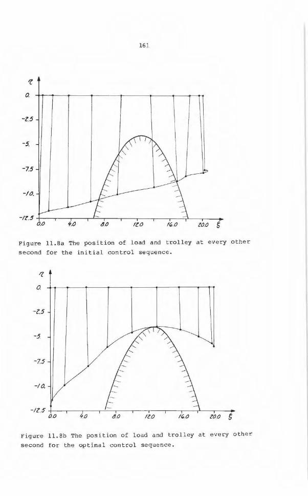
161

0.

-Z.5

-5.

-75

-10.

f.0 8.0 IZO IC..O zo.o 5

Figure 11 . Sa The position o f load and trolley at every other

second for the initial control sequence .

0.

-Z.5

-5.

-7.5

-10.

-/ Z.5 +--.----,----,---:.___--.----,---.---...---...----.l----r--­O.O 8 .0 IZ.O IC..O zoo 5

Figur e ll.8b The position of load a nd trolley at every other

second for the optima l control sequence .

162

Summary

We have shown that our program and the algorithm upon which it is

based is capable of solving non-linear , discre te-time optimal

control problems of different kinds, in particular problems with

state constraints. The program has a l so been appl ied to other

problems, see e.g. Trulsson (1983), and has exposed robust prac­

tical convergence properties .

Comparisons with other numerical schemes, such as DDP show that

our method is competitive. It must however be remarked that it is

difficult to eva l uate comparisons between the continuous-time

DDP-algorithm and our discrete- time algorithm. A fair comparison

should be carried out against a discrete- time counterpart of the

DDP-algorithm, which can handle state constraints. Such an algo­

rithm has, however, apparently never been explicitly reported in

the literature.

The numerical expressions also reveal that some care must be

exercised in the choice of numerical algorithms in the sub­

routines, that mechanize the different equations that are to be

solved in the course of the optimization scheme. Replaci ng the

straightforward implementat ion of the Riccati-equation by more

sophisticated and numerically sound versions is probably the most

important possible improvement of this kind.

163

12 CONCLUSIONS

Many problems in engineering can be formulated as optimization

problems. This thesis focuses on two particular types of optimi­

zation problems, namely nonlinear programming problems, i.e .

nonlinear optimization problems with equal ity and inequality

c onstraints , and optimal control problems in discrete time with

state and control constraints. It has been the aim t hroughout the

thesis to use a unified approach to these two problems .

To that ena an algorithm has been developed which can be looked

a t from two different viewpoints. On the one hand it is exac tly

Wi lson ' s method, i.e. a Newton method for constrained problems,

when the optimal control problem is regarded as a static non-

1 inear optimization problem. On the other hand it is a method

that takes advantage of t he peculiar structure of optimal control

problems and has a form similar to well known optimal control

a lgorithms for problems without state and control constraints . A

benefit from the approach is that it suggests a method of hand­

ling constraints, in particular pure state constraints, which are

notoriously dif ficult t o treat.

To get a deeper understanding of t he relation between the two

points o f view , the regularity conditions of the nonlinear pro­

gramming problem have been interpreted in the optimal control

framework. It has been shown that th e constraint qualification

leads to a cont r ollability condition and that a certain definite­

ness condition can be checked from the behaviour o f a Riccati

equation.

Our approach leads to a simple treatment of convergence ques­

tions. Due to the mathematica l programming interpretation of our

algorithm we have been able to establish bo t h global convergence

and a locally quadratic convergence rate.

A program has been developed which uses our algorithm to solve a

completely genera l nonlinear discrete time optimal control

problem. Both problems that are discrete-time prob l ems in

themselves and problems formulated as piecewise cons tant control

164

af con t inuous-time systems (usually arising from computer cent­

ral) can be handled. The program has been used successfully to

solve a number af prob l ems af varying complexity. Our approach

has thus been shown ta have not only theoretical inte r est, but practical usefulness as well.

165

APPENDIX

SAMPLING OF CONTINUOUS TIME SYSTEMS:

1. Introduction

The main purpose af this thesis is ta describe and analyze a

me thod for solving discrete time nonlinear constrained optimal

c en tral p r oblems . However most af t hese problems originate from

continuous time systems , but are for practical reasons or by

tradition defi ned as discrete time systems . For instance mast

economic sys t ems are usually described as discrete time systems .

Also, when a digital computer is used for controlling a system,

a d i sctcte time description of the sys t em is suitable, because

when a digital computer is used, li1e con t rols a r e usually held

constant between the sample times .

Hence we need a method to get a discrete time description af the

s y stem we are interested in. In this thesis we have assumed that

this discrete time descri p t ion i s given or easily o btained . In

t hi s appendix we will describe how to solve the disc r ete time

descr i p t ion of the system even when it is i mposs i b l e ta e xpli ­

citly f ind t he functions f and l in (4. 1) and ( 4 . 3) .

We assume that we have a contin uous time description of the

system , namely

x('t)=F(x(-c) ,u( 't),'t) ; 02_'t::_tF

a nd t hat wc want to minimize the performance inde x

tF J(u)=l(x(tF) ,tF)+f L(X('t),U('t))d't

0

( A. l)

( A. 2)

We assume that the initial values of the states are given by

x(O) =x0

( A . 3)

166

The problem is now that we are only allowed to change t he values

of t he controls a t certain times, the sampling times.

We will assume here that these sampling times are equidistant

a nd also that the distance between two consequtive sampling

times is 1. (This is not ne cessary. We make these assumptions to

g P. t easier notations). Hence the sampling times are the i ntegers

0,1, . .• ,N-l. we also assume that at these sampling times we have

constraints of the type

hi(x(ti),u(ti)).:_O,i=l, ..• , p. (A.4)

We also assume that the controls are right continuous, i.e.

u(-r)=u(t) if t<-r<t+l. (A.5)

We also assume that the solutions to all the differential

equations in this appendix exist, are uniqe and are bounded on

the intervals on which they a r e defined .

If the state x(t) and the control u(t) are known , we can cal­

culate x(t+l) by solving the differential equa tion (A.l), since

from (A.5) we know the controls u(-r). Hence the function Pin

(A.l) implicitly defines the function f(x(t) ,u(t),1) in the

discrete- time descript ion (4.1) of t he system. Also in (4.3) the

values of the function l(x(t),u(t},t) could be evaluated as

t +l l(x(t) ,u(t) , t)= f L(x(-r) , u(-r),-r)d-r

t ( A. 6)

So we conclude that th~ prob lem defined by (A.1-5) is actually

of t he same type as that described in chapte r 4, but usually the

functions f and l a re imposs ible to ge t explici tly.

In the following we wi ll use the notations a(t+) and a(t ) when

we mean the right hand lim i t and the left hand limit o f the

piece- wise continuous funct ion a(t) .

Hence i f E >O we ha ve

a(t+)=lim a(t+e) e+O

a(t )=lim a(t-e). e+O

167

(A.7a)

( A. 7b)

In the next section we derive the necessary equations when there

are no constraints of the type (A.4) and in section 3 we extend

these resul ts to include these constraints .

2. Solving the unconstrained problem

We will derive a technique for solving the optimal control,

def ined in the previous section. When we derive this technique

we will c losely follow the same lines as those in section 4. 3 .1,

when we derived the technique for discrete time systems. Con­

sequently we let z(t) consist of the controls from time t up to

N- 1 as i n (4.6). Hence

T T T z ( t) = ( u ( N-1) I • •• I u ( t) ) • (A. 8)

In (4.8) we defined the function V(x(t),z(t) ,t) as the cost from

time t up to time N starting at x(t) and using the control

defined by z(t). So here we, for t~i:<t+l, define

N V(x(i:) ,z(t) ,i:)=1(x(N) ,N)+ f L(x(s) ,u(s) ,s)ds

't ( A . 9)

where x(s), for s~i:, is the solution to (A.l) starting at x(-t),

and u(s) is defined by (A.8) and (A.5) . As in section 4.3.1 we

now want to calculate the derivatives of V(t+) with respect to

x, z, xx, xz, and zz. We do that in the following way. The de­

rivative of the function V('t) in (A.9) with respect to 't is

. V('t)=V't('t)+Vx(i:)F('t}=-L('t) (A.10)

if t<i:<t+l. (The term Vz(i:)~(t) in the expression above vanishes

because z(t) is inde pendent of • on the interval . )

168

From {A.10) we get the equality

V (t)+L{•)+V {•)F{•l=O. 't X ( A.11)

By differentiating (A.11) with respect to x, z, xx, xz and zz we

get the following equalit ies.

{A.12a)

(A.12b)

(A.12c)

(A.12d)

v ( • l+ (oo ZZ't LO{•)) +FT{'t)Vxzz{•)+ (FT( •~V (•)\+ uu u xz ~

+ ( 0 I V ( 't) E' ( 't) ) + ( 0 0 ) =O ZX U 0 V X ( 't) F UU ( 't )

{A.12e)

Using the equali t ies in (A.12) we can derive t he following

differential equalities in the interval t<•<t+l.

• T -V (•)=-V (•)- E' ('t)V ('t)=L (•)+V (•)F ('t) X X't XX X X X {A.13a)

(A.13b)

• T T - V (-i) =-V {'t)-F (• )V (<) =L (-i)+F (•)V (•) XX XX't XXX XX X XX

+V ('t)F (-i)+V (•) F (•) XX X X XX (A.13c)

169

(A.13d)

= (OT ) + (0, V (-i-)f' (-i-))+ (00 f' (-i-)V ('t") zx u

u xz

(A. 13d)

From the definition (A . 9) o f the function V('t") and the construc­

tion (A.8) of the vector z(t), it is obvious that we have the

following boundary conditions .

V (N-)=O z

V (N-)=0 zz

and for t=l, . . . , N-1 we have

- + V (t )=(V (t ),0)

xz xz

(A .14a)

(A . 14b)

(A. 14c)

(A.14 d)

(A . 14e)

(A . 14f)

(A.14e)

(A. l4g)

(A . 14h)

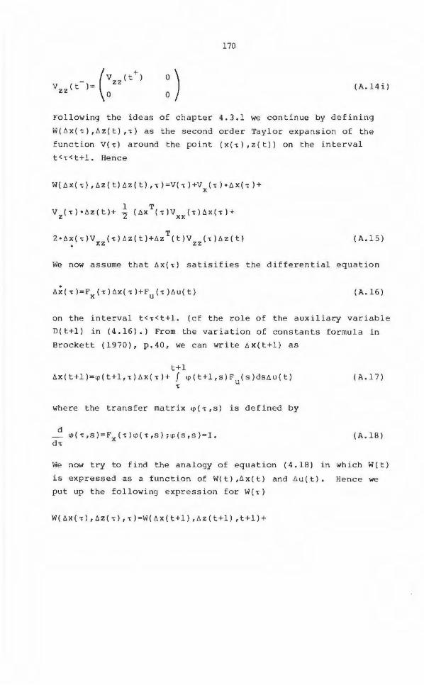
170

: ) (A. 1 4 i)

Followi ng the i deas of c hapter 4.3.l we continue by defining

W(öx(•),öz( t) ,•) as the second order Taylor expansion of the

f unc tion V(•) around the point (x(•) ,z(t) ) on the interval

t <• <t+l . Hence

W( 6X( ') , 6Z ( t) 6Z ( t) , ')=V(') +V X (') • 6 X(' ) +

( A.15)

We now assume that öx (•) satisi f ies the di f ferential equation

( A.16)

on t he interval t<•<t+l. (cf the role o f the auxiliary variable

D(t+l) in (4. 1 6) .) From the variation of constants formula i n

Brockett (1970) , p. 40, we can write öx(t+l) as

t+l 6x (t +l )=~(t+l, ,)6x ( •) + f ~(t+l , s)F (s)dsöu(t}

u

where the transfer matr i x ~ ( , , s ) is def ine d by

( A. l 7 }

d ~ (•, s}=Fx(• )~( • ,s); ~(s ,s) = I . (A.18)

d•

We now try to fi nd the ana logy of equation (4. 18 ) in which W(t)

is expressed as a function of W(t) ,öx(t) and 6 u(t). Hence we

put up the following expression for W(•}

W ( 6 X ( ') , 6 Z ( ' } , ' ) =W ( 6 X ( t + 1} , 6 Z ( t + l) , t + 1 ) +

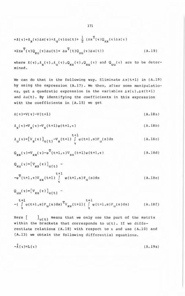
171

T T +2llx ('t)Q ('t)Au(t)+ AU (t)Q ('t)AU(t )) xu uu (A . 19)

where ..t('t) ,..t ('t) ,..t ('t) ,Q ('t) ,Q ('t) and Q ('t) are to be deter-x U XX XU UU mined .

We can do that in the f ollowing way. Elimi nate ö x(t+l) in (A.19)

by using the expression (A . 17) . We then, af t er some manipulatio­

ns, get a quadratic expression in t he variables AX ('t), llz ( t+l)

and llu(t). By identifying the coefficients in this expression

with the coefficients in (A.15) we get

..t('t)=V('t}-V(t+l)

..t ('t)=V ('t)-V (t+l)11>(t+l,'t) X X X

t+l ..t ('t)=[v ('t)] (t)-v (t+l) f 11> (t+l ,s )F ( s)ds

U Z U X U 't

Q ( 't)= [ V ('t)) -xu xz u{t)

t+l -11>T{t+l,'t)Vxx(t+l) J 11> (t+l,s)Fu(s)ds

't

t+l T t+l -( f 11>(t+l,s)Fu(s)ds) Vxx(t+l){ f 11> (t+l , s)Fu (s)ds)

't 't

(A.18 a )

(A.18b)

( A.18 c )

(A . 18d)

(A . 18e )

( A. 18 E)

Here ] u(t) means t hat we only use the part of the matrix

within the brackets that corresponds to u(t). If we diffe ­

rentiate relations (A . 18) with respect to 't and use (A.10) and

(A.13) we obtain the following di ffe rential equations •

. -..t(.) =L('t) (A . 19a)

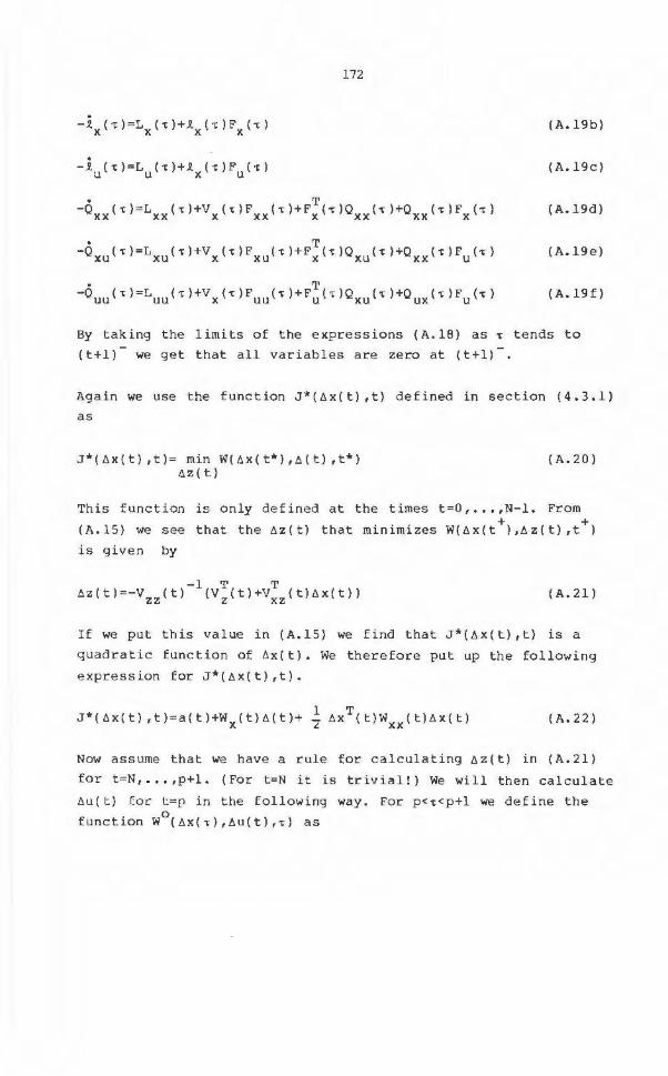
172

-1 (-c)=L (-c)H (•)F (-c) X X X X

(A.19b)

-1 (-c)=L (-c)+~ (-c)F (-c) U U X U

(A.19c)

(A. 19d)

( A.19e)

• T -Q (-c)=L (-c)+V (-c)F (-c)+F (•)Q (-r) +Q (•)F (-c) UU UU X U U U XU UX U

(A.19 f)

By taking the limits of the expressions (A.18) as• tends to {t+l) we get that all variables are zero at (t+l)-.

Again we use the func t ion J*(6x(t) ,t) defined in section (4.3.l) as

J*(6x(t) , t)= min W(6x(t*),6(t) ,t*) 6z( t)

(A.20)

This function is only defined at the times t=O , .•. ,N-1. From

(A.15) we see that the 6z(t) that minimizes W(6x(t +),6z(t) ,t+)

is given by

(A .21)

If we put this va lue in (A.15) we fina that J*(6x(t) ,t) is a

quadratic function of öx(t). We therefore pu t up the following

expression for J*(6x(t),t).

J * ( 6 X ( t ) , t ) = a ( t ) +W X ( t ) 6 ( t ) + ~ 6 X T ( t ) W X X ( t ) 6 X ( t ) ( A • 2 2 )

Now assume that we have a rule for calculating öz(t) in (A.21)

for t=N, • .. , p+l. (For t =N it is triv i a l!) We will then calculate

öu( t) r:oc t=p in the following way. For p<-r<p+l we defi ne the

function w0 (öx(-c),6u(t),-r) as

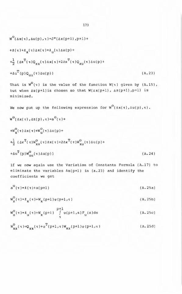
173

w0 (öX(<),öu(p),•)=J*(öx(p+l) ,p+ l )+

+l{T)+l (T)AX(T) +l (T)öu(p)+ X U

(A. 23)

That is w0(•) is the va lue of the function W(•) given by (A.15),

but when 6z{p+l)is chosen so that W(öx(p+l), öz(p+l) , p+ l) is

minimi zed .

We now put up the f ollowing expression for w0 (öx(>) , öu(p),T).

0 0 W ( Ax ( • ) , A z ( p) , • ) =a ( • ) +

(A . 24)

If we now again use the Variation of Constants Formula ( A.17) to

eliminate the variables Ax(p+l) in (a . 23) and identify the

coeff icients we ge t

a 0 (•)=1(•)+a(p+l) (A. 25a)

w0 (•)=1 (>)+W (p+l)~(p+l,>) X X X

(A . 25b)

p+l w0 (•)=1 (•)+W (p+l) J ~(p+l ,s)F (s )ds

U U X U ( A. 25c)

T

o T W (<)=Q (T)+~ (p+l,T)W (p+l)~(p+l,T)

XX XX XX (A.25d)

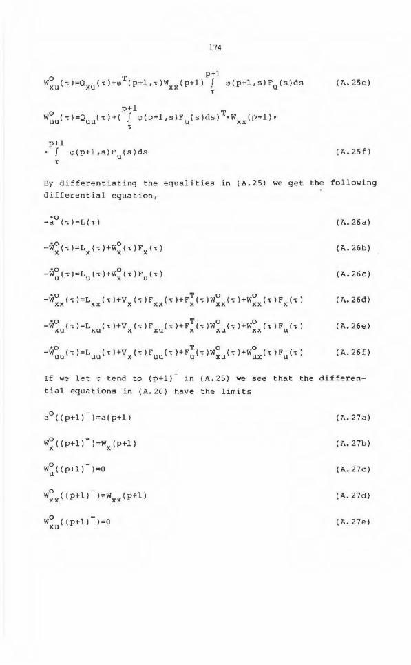
174

p+l T W~u('t)=Quu('t) + ( f 11>(p+l,s)Fu(s)ds) ·Wxx(p+l)•

't

p+l • f

• 11>(p+l, s)F (s)ds

u

(A.25e)

(A.25f)

By differentiating the equalities in (A.25) we get the following

differential equation,

•O -a ( >) =L ( 't ) (A . 26a)

(A.26b)

(A.26c)

(A.26d )

(A.26e)

(A.26f)

If we let • t e nd to (p+l) in (A . 25) we see that the differen­

t i al equations in (A . 26} have the limits

0 -a ((p+l} )=a(p+l}

w0 ((p+l)-}=W (p+l} XX XX

w0 ( ( p+ l ) - ) = 0

xu

(A.27a}

(A . 27b}

(A.27c)

(A.27d)

(A.2 7e)

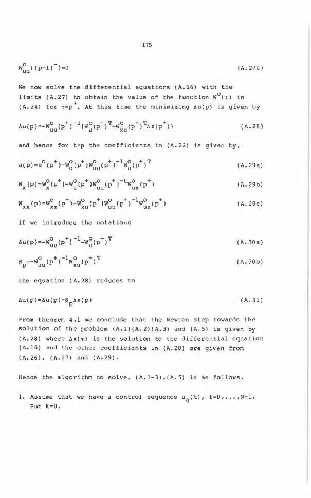
w0 ( (p+l)-)=0

uu

175

(A. 27f)

We now solve the differential equa tions (A.26) with the

limits (A.27) to obtain t he va lue of the function w0 (• l in + (A.24) for •=p . At this time the minimizing tiu(p) is given by

o + -1 o + T o + T + tiu(p)=-Wuu(p ) (Wu(p ) +wxu(p ) tix(p )) (A.28)

and hence for t=p the coefficients in (A.22) is given by,

w ( )-wo ( +)-wo ( +)Wo ( +,-1wo ( +} XX p - XX p XU p UU p UX p

if we introduce the notations

the equation (A.28) reduces to

tiu(p)=öu(p) -~ tix(p) p

(A.29a)

(A.29b)

(A.29c)

(A . 30a)

(A. 30b)

( A. 31)

From theorem 4.1 we conclude that t he Newton s t ep towards the

solution of the problem (A.l)(A.2)(A.3) and (A. 5 ) is given by

(A.28) whe re tix(•) is the solution to the differential equation

(A.16) and the other coefficients in (A.28) are given from

(A.26), (A.27) and (A.29).

Hence the algorithm to solve, (A.l-3),(A.5) is as follows .

1. Assume that we h ave a control sequence u0(t), t=O, .. . ,N-1.

Put k=O.

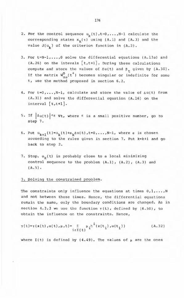
176

2. For the control sequence uk(t),t=O, •• . ,N-1 calculate the

corresponding states xk(•) using (A.l) and (A.3) and the

value J(uk) of the crite r i on function in (A . 2).

3. For t=N-1, .•• ,0 solve the d iffe r e ntial equations (A. 13a) and

(A.26) on the intevals [t,t+l ] . During these ca l culations

compute and store t he values of öu(t) and ~t given by (A.30).

If the mati:-ix W~u(t+) becomes singular or indefinite foi:- some

t, use the method propos ed in section 6.2.

4 . For t=O, •.. ,N-1, c alculate and stor e the value of ti u ( t) from

(A.31 } and solve the d ifferential equation (A.16) on the

interval [t,t+l].

5. If l6u(t) l<e Vt, where E is a small positive number, go to step 7.

6. Put uk+l(t}=uk(t)+aktiu(t) ,t=O, •.• ,N-1, where a is chosen

accoi:-ding to the rules given in section 7. Put k=k+l and go

back to step 2.

7. Stop. uk(t} is probab l y close toa local minimizing

control sequence to the problem (A.l), (A.2), (A.3) and

( A. 5).

3. Solving the constrained problem.

The constraints only in fl uence the equations at times 0,1, •.• , N

and not between these time s. Hence, the diff e rential equations

remain the same, on l y t he boundary conditions a re change d. As in

section 4.3.3 we use the f unction y(t), defined by (4.50), to

obtain the influence on the constraints. Hence,

i y(t)=y(x(t) ,u(t}, µ ,t)= E µ .h (x(t.) ,u(t . )} i e l(t) 1 1 1

( A. 32)

where I(t) is defined by (4.49). The va l ues of µ are t he ones

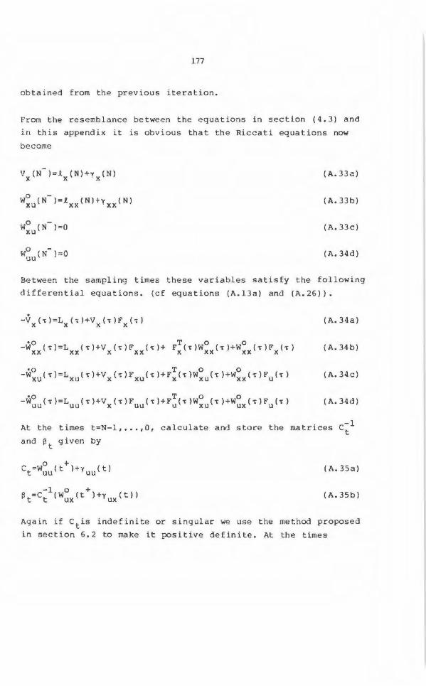
177

obtained from the previous iteration .

From the resemblance between the equations in section (4 . 3) and

in this appendix it is obvious that the Riccati equations now

become

w0 (N-)=1 (N)+y (N) XU XX XX

w0 (N-)=0 uu

(A.33a)

(A.33b)

(A . 33c)

(A.34d)

Between the sampling times these variables satisfy the following

differential equations. (cf equations (A.13a} and (A . 26)).

(A . 34a)

(A . 34b)

(A. 34c)

(A.34d)

At the times t=N-1, . . . ,0, calculate and store the matrices c~ 1

and ~t given b y

(A.35a)

(A . 35b)

Aga in if Ctis indefinite or singular we use the method proposed

in sect ion 6.2 to make it positive definite . At the times

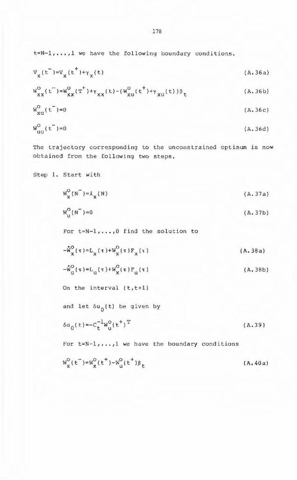
178

t =N-1, . . . , l we have the following boundary conditions.

w0 (t- ) =0 xu

(A.36a)

( A. 36b)

( A. 36c)

(A.36d)

The trajectory corresponding to the uncons trained o ptimum is now

obtained from the following two steps.

Step l. Start with

w0 (N-)=O u

For t =N-1, ... ,0 find the solution to

On the interval (t,t+l )

and let ou0

(t) be given by

For t=N- 1, . .. ,l we have the boundary conditions

(A . 37a)

(A. 37b)

(A.38a)

(A.38b)

( A. 39)

(A.40a)

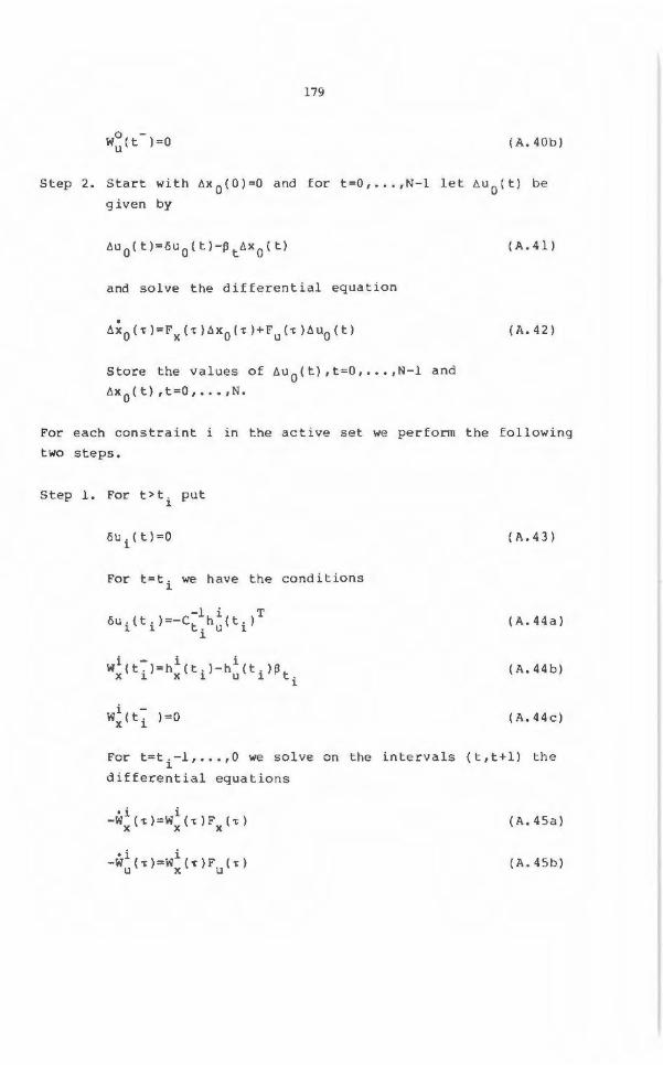
179

(A . 40b)

Step 2. Start with Ax 0 (0)=0 and for t=O, .. . ,N-1 let Au0

(t) be

given by

and solve the d i fferential equation

. Ax 0 (~)=Fx(~)Ax 0 (~)+Fu(~)Au0 (t)

Store the values of Au0(t),t=O, . .. , N-l and

Ax0

( t) ,t=O, • .. ,N .

(A. 41)

(A . 42)

For each constraint i in the active set we perform the following

two steps .

Step 1. For t>ti put

öui(t ) =O (A . 43)

For t= t i we have the conditions

(A . 44a)

(A. 44b)

(A.44c)

For t=ti-1, .•. , 0 we solve on t he interva l s (t , t+l) the

differential equations

(A . 45a)

(A . 45b)

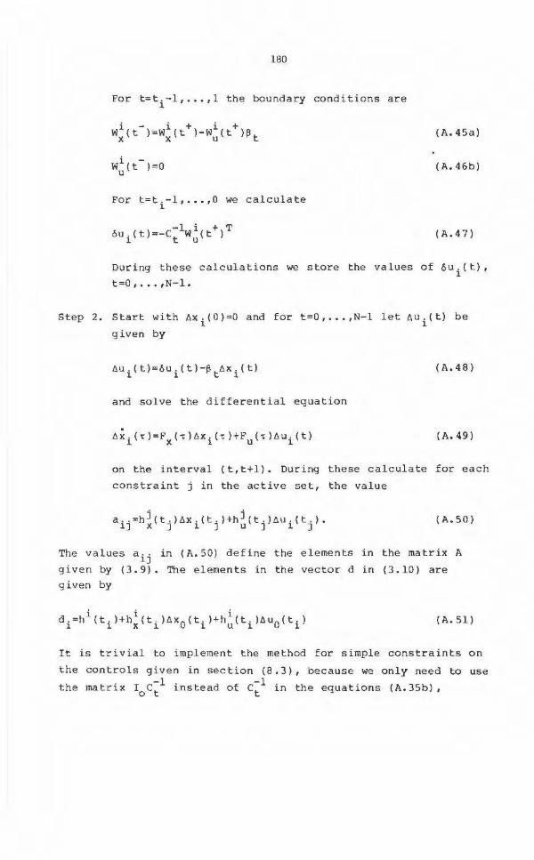
180

For t=ti - 1, ... ,1 the boundary conditions are

{A.45a)

{A. 46b)

For t =ti-1, .•• ,0 we calculate

( A. 4 7)

During these calculations we store the values of öu i ( t), t=O, ... ,N-1 .

Step 2. Start with Axi(O)=O and for t=O, ••• ,N-1 let AUi{t) be

given by

L'I U. { t) =ÖU. { t )-j'l tL'IX . ( t) l l l

(A .48 )

and solve the differential equation

A~.('t)=F ('t)AX.('t)+F ('t)L'lu.(t) l X l U l

(A. 49)

on the interval {t,t+l ). During these calculate for each

constraint j in the active set, the value

a .. =h j ( t.) AX. ( t. )+h j ( t.) AU . ( t.). lJ X J l J U J l J

(A.50)

The values a .. in (A.50) define the elements in the matrix A l J

given by (3.9). The elements in the vector d i n (3.10) are given by

(A. 51)

It is trivial to impl ement the method for simple constraints on

the controls g iven in section (8.3), because we only need to use

the matrix r0c~1 instead of c~ 1 in the equations (A.35b),

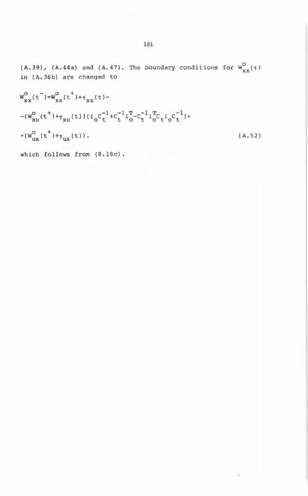
181

(A . 39) , (A.44a) and (A .4 7) . The boundary conditions for w~x('t) in (A.36b) are c h anged to

( A . 52)

which follows from (8 . 18c).

182

183

REFERENCES

Arri a tti, eds . {1971)

Preliminary report on optimization studies . CIGRE Study Committee

32 . Working Group Al . Rome April 8th, 1971.

Bartels , R.H., G.H. Golub and M.A. Saunders . (1970)

Numerica l Techniques in Mathematical Programmi ng . In J . B. Rosen,

O. L. Ma ngasarian a nd K. Rit t er , eds., Nonlinear Programming,

Academic Press, Ne w York, pp . 123-176 .

Bellman, R.E. and S.E . Dreyfus. (19 62)

Applied Dynamic Programming. Princeton University Press ,

Princeton.

Bertsekas, D. P . (1982)

Constrained Optimization a nd Lag r ange Multiplier Methods.

Academic Press, New York.

Brockett, R.W. ( 1970)

Finite Dimens ional Linear Systems. John Wiley and Sons Inc . , New

York.

Bryson, A. E. and Y. - C. Ho . { 1969)

Applied Optimal Con trol . Ginn and Company, Waltham , Mass .

Bunch, J . T. and L. Kaufman (1980)

A Comp utational Method for t he Indefi ni te Quadratic Pr ogramming

Problem . Linear Algebra Applications , Vol. 34 , pp. 348-370 .

Canon , M. D., C. D. Cullum and E. Po l ak {1970)

Theory of Optimal Control and Mathematical Programmi ng . McGraw­

Hill Book Company, New York.

Chamberlain, R. M. , C. Lemarechal, H. C. Pedersen and M. J . D.

Powell (197 9)

The Watchdog Technique for Forcing Convergence in Algorithms for

Constra ined Optimization. Tenth International Symposium on

Mathematical Programming, Montreal, August 1979.

184

Dahlquist, G. and A. Björck (1974)

Numerical Methods. Prentice-Hall Inc. , Englewood Cliffs , New

Jersey.

Dyer, P. and S.R. McReynolds (1970)

Th e Computa tion and Theory of Optimal Control. Academic Press,

New York.

E'letcher, R. (1980)

Practical Methods of Optimization. Volume 1. John Wiley and

Sons, New York.

E'le tcher, R. ( 1981)

Practical Methods of Optimization. Volume 2. John Wiley and

Sons, New Yo rk.

Gill, P.E. , G.H. Golub, w. Murray and M.A. Saunders (1974)

Methods fo r Modifying Matrix E'actorizations. Mathematics of

Computa tion, Vol. 28, No. 126 pp. 505 - 535.

Gill, P . E. and w. Murrary (1978)

Numer ical l y Stable Methods fo r Quadratic Programming.

Mathematical Programming, 14, pp. 349- 372.

Gill, P.E., w. Murrary and S.M. Picken. (1972)

The Implementation of Two Modified Newton Algorithms for

Unconstrained Optimization. NPL Report NAC24.

Goldfarb, D. ( 1975)

Matrix Factorizations in Optimization of Nonlinear Functions

Subject to Linear Constra i nts. Mathematical Programming 10, pp.

1-31.

Han, S.-P. (1975)

Superlinearly Convergent Variable Metric Algorithms for General

Non linea r Programming Problems. TR 75-233, Cornell University.

185

Han, S.-P . (1977)

A Globally Convergent Method for Nonlinear Programming. TR 75-

257, Cornell University . / J. of Optimization Theory and

Applications, Vol. 22, pp. 297-309 .

Jacobson, D.H. and D. Q. Mayne ( 1970)

Differential Dynamic Programming . American Elsevier Publishing

Company, Inc., New York, 1970 .

Jirmark, B. S . A. (1976)

Convergence Control in Differential Dynamic Programming Appli e d

to Air-to-air Comba t. AIAA J. 14(1), pp. 118-121.

Kwakernaak, H. and R. Sivan (1972)

Linear Optimal Control Systems. Wiley-Interscience, New York .

Lasdon, L. S . ( 19 79)

Optimization Theory for La r ge Sys t ems . MacMillan Publishing

Company Inc., New York.

Luenberg er, D. G. ( 1973)

Introduction to Linear and Nonlinear Pro g ramming . Add ison

Wesley, Reading, Mass .

Luenberger , D.G. (1979)

Introduction to Dynami c Systems . John Wiley and Sons, New York .

Mayne, D. (1966)

A Second-Order Gradient Method fo r Determining Optimal

Trajectories of Non-L inear Discrete-Time Systems . Int. J.

Control , Vol . 3, No.l, pp. 85-95.

McRe ynolds , S.R. and A. E. Bryson. ( 1965)

A Successive Sweep Method for Solv ing Optimal Programming

Problems . Joint Autom. Control Conf ., pp. 551-555. Troy, New

York, June 1965.

Mitter, S,K. (1966)

Successive Approximation Methods for the Solution of Optima l

Control Problems. Automatica, Vol. 3, pp . 135-149.

186

Ohno, K. (19 78)

A New Approach t o Differential Dynamic Prog ramming for Discrete

Time Systems. IEEE Trans. on Automatic Control , Vol. AC-23, No.

l , pp . 3 7 - 4 7 •

Paige , C.C. and M.A. Saunders ( 1975)

Solution of Spa r se I ndefinite Systems of Linear Equations. SIAM

J. Numer. Anal. Vol. 12, No. 4, pp. 617-629 .

Polak, E. ( 1973)

An Historical Survey of Compu t ational Methods in Optimal

Control. SIAM Re vi e w, Vol . 15, No.2, pp. 553-584.

Powell, M.J.D. (1978)

A Fast Al gorithm for Nonlinearly Constrained Optimization. In

Numerical Analysis, Dunde e , 1977, Lec t ure Notes in Mathematics

630. Springer Verlag, Berlin, pp. 144 -1 57.

Powell, M.J.D. (1981)

An Upper Triangular Matrix Method for Quadratic Programming. In

O.L. Mangasarian et.a l . eds., Nonlinear Programming 4. Academic

Press, New York . pp.l-24.

R ud in, W. ( l 9 6 4 )

Principles of Mathematica l Analysis. 2nd ed. McGraw-Hill Book

Company, New York.

Talu kdar, S . N. and T.C. Giras (1982)

Robust Variabl e Metric Method for Optimum Power Flows. IEEE

Trans Power Apparatus and Systems , Vol PAS-101 No 2.

Trulsson, E. ( 1983)

Adapt i ve Control based on Explicit Criterion Minimization.

Ph.D. Dissertation, Linköping University

Wilson, R.B. ( 1963)

A Simpl icial Method for Concave Programming. Ph. o. dissertation,

Harvard Un iversi ty, Cambridge, Mass.