NL senior conference paper (1)

QUANTIFYING THE HOPE FOR REDUCING BIAS IN THE SOCIALSCIENCES

NIKHITA LUTHRA

1. INTRODUCTION

1.1. Motivation. The sixth highest killer of Americans is Alzheimer’s Disease. This fatal

neurological disease has stumped researchers from wealthy countries for over two hundred

years. A recent discovery, however, o↵ers hope to the one-in-three senior citizens who will

develop the disease. Surprisingly, that hope doesn’t come from the white walls of a medical

center at a well endowed research university in the States; it comes from the remote hills

of Antioquia, a village outside Medellin, Colombia. After going through historical priests’

records at local churches, Dr. Francisco Lopera of Medellin’s University of Antioquia dis-

covered that members of a particular family had recorded early onset of Alzheimer’s for over

300 years. More research revealed that in this family, a person has a 50 percent chance of

inheriting a gene, PSEN1, that guarantees early onset of Alzheimer’s. After the National

Health Institute picked up word of this once in a lifetime experiment opportunity, resources

were quickly gathered to run clinical trials on an antibody that targets the protein amyloid

which is associated with the disease.

The unearthing of this family o↵ers a researcher’s dream: the perfect conditions to run

a natural experiment. Because subjects and researchers didn’t want to know which members

of the family carried the fatal gene, they could randomly apply treatments in a double blind

setting. A double blind study is when neither the subjects or the researchers know which

groups subjects are assigned to. In addition, the fact that members of the family had mostly

stayed in the same location with similar living situations meant that variables that di↵er

based o↵ location of residence could be controlled for.

Most researchers are not as lucky to find the perfect conditions to infer that a treatment

caused the prevention or cure of a disease. In the real world, treatments tested in the social

sciences are conditionally dependent on covariates. For example, in medicine, drugs are only

tested on sick patients. In economics, researchers test a welfare benefit on the disadvantaged.

Without randomization, selection bias arises: are di↵erences in the outcome caused by the

selection of who is in the treatment group rather than the treatment itself? This inability

to infer causality has plagued social scientists for decades.1

2 NIKHITA LUTHRA

1.2. Overview. Luckily, statistics o↵ers some solutions to overcome the inability to ran-

domly apply treatments. When random assignment is missing, matching samples based on

particular variables attempts to reduce the bias of estimates of treatment e↵ects. Recent

literature has focused on matching methods that attempt to reduce the bias of confounding

variables that systematically di↵er between control and treatment populations. Rather than

focusing on various matching methods, we will derive two values, ✓ and ✓

max

, which are used

to evaluate the success of a matching method, both for the situation when we want to reduce

the bias of a single variable (section 2) and also when we want to reduce the bias of many

covariates (section 3). To do this, we will first describe how to estimate the treatment e↵ect

on a particular outcome variable. Then, we will construct ✓, which captures the reduction

in bias of an estimator due to matching. Finally, we will derive ✓max

, the maximum

percent reduction in bias. This value is important because it intuitively acts as an up-

per bound on how much hope we can have in matching’s ability to reduce bias, ultimately

“saving” the social sciences from their inability to infer causality.

2. MATCHING ON ONE VARIABLE

When is it the case that adjusting for some variable X or variables X gives unbiased

estimates of the treatment e↵ect? This happens whenever the treatment assignment is

strongly ignorable. If r1 is the outcome after receiving the treatment and r0 is the outcome

after not receiving the treatment, treatment assignment is strongly ignorable when: (i) the

responses (r1, r0) are conditionally independent of the treatment z given X and (ii) at each

value of X, there’s a positive probability of receiving each treatment [3]. These conditions

are represented mathematically:

Pr(r1, r0, z|X) = Pr(r1, r0|x)(Pr(x|X)) and

0 < Pr(z = 1|X) < 1 for all possible X.

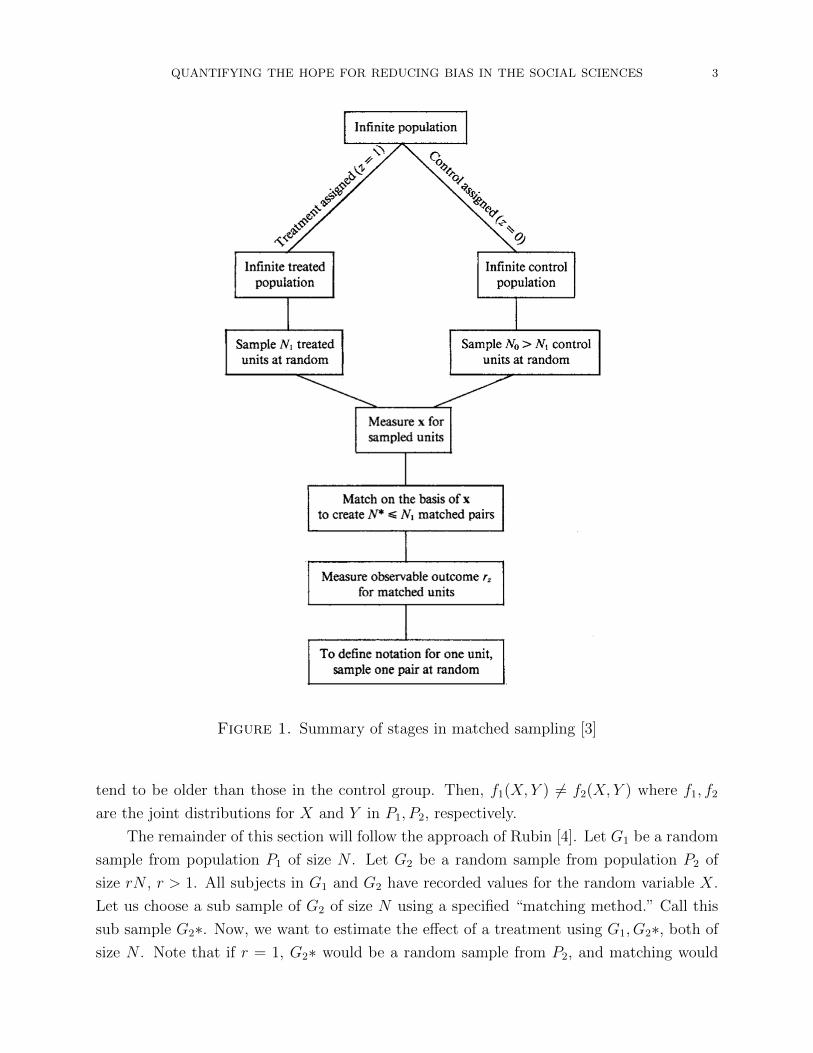
Thus, the goal of matching is to construct samples that make treatment assignment as

ignorable as possible. Figure 1 gives an overview of the process of matching.

2.1. Estimating the treatment e↵ect. Imagine the situation where we are interested in

testing the e↵ect of a particular drug on reducing cholesterol levels, represented by Y , a

continuous dependent variable. We begin by assuming that we only have 1 variable, X, to

match on. For example, let X be the age of a patient. We assign X = 1 for patients over 50

years of age and X = 0 for patients under 50 years of age. We want to remove the e↵ect of X

on Y . Suppose we have two populations, P1 and P2, where P1 is the population of patients

that will receive the treatment (because they have high cholesterol), and P2 is the population

of patients that will not receive the treatment (also known as the control population). The

distribution of the matching variable X di↵ers in P1 and P2; patients in the treatment group

QUANTIFYING THE HOPE FOR REDUCING BIAS IN THE SOCIAL SCIENCES 3

Figure 1. Summary of stages in matched sampling [3]

tend to be older than those in the control group. Then, f1(X, Y ) 6= f2(X, Y ) where f1, f2

are the joint distributions for X and Y in P1, P2, respectively.

The remainder of this section will follow the approach of Rubin [4]. Let G1 be a random

sample from population P1 of size N . Let G2 be a random sample from population P2 of

size rN , r > 1. All subjects in G1 and G2 have recorded values for the random variable X.

Let us choose a sub sample of G2 of size N using a specified “matching method.” Call this

sub sample G2⇤. Now, we want to estimate the e↵ect of a treatment using G1, G2⇤, both of

size N . Note that if r = 1, G2⇤ would be a random sample from P2, and matching would

4 NIKHITA LUTHRA

not be able to remove bias due to X. If r = 1, then infinite matches would be obtained,

and all bias due to X could be removed.

Definition 1. Define the response surface for Y in P

i

at X = x, denoted R

i

(x) as such:

R

i

(x) = E(Y |X = x).

In our example, R1(old) = E⇥cholesterol level | old

⇤gives the expectation of the choles-

terol level for the treatment group given that the patient is old. R2(old) = E⇥cholesterol

level | old⇤gives the expectation for the cholesterol level for the control group given that the

patient is old. R1(young) = E⇥cholesterol level | young

⇤gives the expectation for the choles-

terol level for the treated group given that the patient is young. R2(young) = E⇥cholesterol

level | young⇤gives the expectation for the cholesterol level for the control group given that

the patient is young.

Definition 2. The e↵ect of the treatment at X = x is: R1(x)�R2(x).

Following our example, R1(old) � R2(old) reveals the e↵ect of the treatment among

the old patients. It is the expected cholesterol levels for old people who received the treat-

ment minus the expected cholesterol levels for old people who didn’t receive the treatment.

R1(young) � R2(young) reveals the e↵ect of the treatment among the young patients. It

is the expected cholesterol level for young people who received the treatment minus the

expected cholesterol level for young people who didn’t receive the treatment.

There are two possible cases for the e↵ect of the treatment. The e↵ect of the treatment

can be constant or it can vary with x. These two cases, also referred to as “parallel” and

“non parallel” response surfaces, are defined.

Definition 3. If R1(x)�R2(x) is constant and independent of X, we call R1(x) and R2(x)

“parallel” response surfaces. In this case, the goal is to estimate this constant di↵erence.

Parallel response surfaces are depicted in Figure 2.

Definition 4. If R1(x) � R2(x) is not constant across all values of X, we call R1(x) and

R2(x) “non parallel” response surfaces. In this case, the goal is to estimate the average

di↵erence between R1(x) and R2(x) across all x. Non parallel response surfaces are depicted

in Figure 3.

Definition 5. In both cases, we are interested in estimating the treatment e↵ect among

the control and treated populations, ⌧ , which is equal to the expected di↵erence in the

response surface: ⌧ = E1

⇥R1(x)�R2(x)

⇤.

Allow y1j, x1j to represent the values of Y , X for the jth subject in G1 and y2j, x2j

to represent the values of Y , X for the jth subject in G2⇤, where j = 1...N . Then y

ij

=


Figure 2. Parallel uni variate response surfaces [4]

Figure 3. Nonparallel uni variate response surfaces [4]

R

i

(xij

)+ e

ij

, i = 1, 2; j = 1...N . Ec

(eij

) = 0. Ec

= the conditional expectation given the xij

.

We can use this notation to now express an estimator for the treatment e↵ect that is based

o↵ of data we can actually collect from our sub samples.

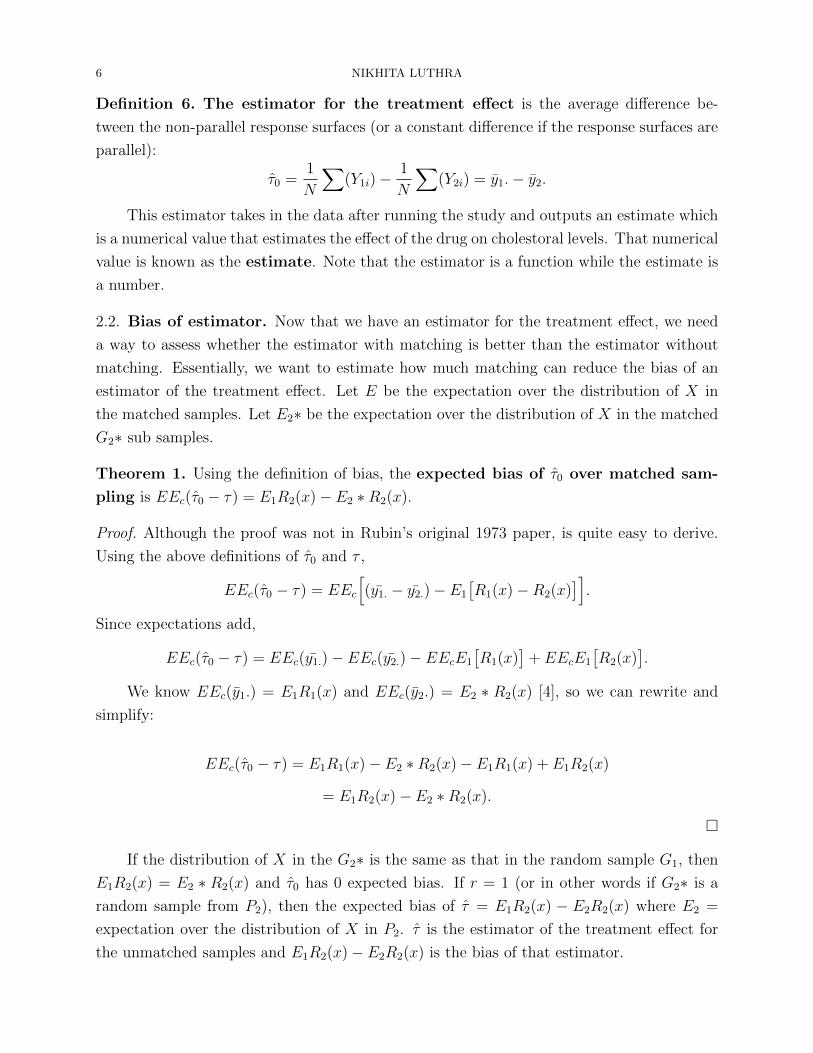
6 NIKHITA LUTHRA

Definition 6. The estimator for the treatment e↵ect is the average di↵erence be-

tween the non-parallel response surfaces (or a constant di↵erence if the response surfaces are

parallel):

⌧0 =1

N

X(Y1i)�

1

N

X(Y2i) = y1.� y2.

This estimator takes in the data after running the study and outputs an estimate which

is a numerical value that estimates the e↵ect of the drug on cholestoral levels. That numerical

value is known as the estimate. Note that the estimator is a function while the estimate is

a number.

2.2. Bias of estimator. Now that we have an estimator for the treatment e↵ect, we need

a way to assess whether the estimator with matching is better than the estimator without

matching. Essentially, we want to estimate how much matching can reduce the bias of an

estimator of the treatment e↵ect. Let E be the expectation over the distribution of X in

the matched samples. Let E2⇤ be the expectation over the distribution of X in the matched

G2⇤ sub samples.

Theorem 1. Using the definition of bias, the expected bias of ⌧0 over matched sam-

pling is EE

c

(⌧0 � ⌧) = E1R2(x)� E2 ⇤R2(x).

Proof. Although the proof was not in Rubin’s original 1973 paper, is quite easy to derive.

Using the above definitions of ⌧0 and ⌧ ,

EE

c

(⌧0 � ⌧) = EE

c

h(y1. � y2.)� E1

⇥R1(x)�R2(x)

⇤i.

Since expectations add,

EE

c

(⌧0 � ⌧) = EE

c

(y1.)� EE

c

(y2.)� EE

c

E1

⇥R1(x)

⇤+ EE

c

E1

⇥R2(x)

⇤.

We know EE

c

(y1.) = E1R1(x) and EE

c

(y2.) = E2 ⇤ R2(x) [4], so we can rewrite and

simplify:

EE

c

(⌧0 � ⌧) = E1R1(x)� E2 ⇤R2(x)� E1R1(x) + E1R2(x)

= E1R2(x)� E2 ⇤R2(x).

⇤

If the distribution of X in the G2⇤ is the same as that in the random sample G1, then

E1R2(x) = E2 ⇤ R2(x) and ⌧0 has 0 expected bias. If r = 1 (or in other words if G2⇤ is a

random sample from P2), then the expected bias of ⌧ = E1R2(x) � E2R2(x) where E2 =

expectation over the distribution of X in P2. ⌧ is the estimator of the treatment e↵ect for

the unmatched samples and E1R2(x)� E2R2(x) is the bias of that estimator.


2.3. Measuring reduction in bias due to matching. Now we wish to determine how

much less biased the ⌧0 based on matched sampling is compared to the ⌧ based on ran-

dom sampling. We will use the “percent reduction in expected bias” to measure this. It

is essentially the expected bias for matched sampling over the expected bias for random

sampling:

100⇣1� E1R2(x)� E2 ⇤R2(x)

E1R2(x)� E2R2(x)

⌘.

The numerator, E1R2(x) � E2 ⇤ R2(x), represents the expected bias from matched sam-

pling and the denominator, E1R2(x) � E2R2(x), represents the expected bias from random

sampling. The terms that di↵er are E2R2(x) and E2 ⇤ R2(x). Multipling by a common

denominator and simplifying yields the expression:

100⇣E2 ⇤R2(x)� E2R2(x)

E1R2(x)� E2R2(x)

⌘

We can see from this equation that the percent reduction in bias depends only on the

distribution of X in P1 and P2 and G2⇤ and the response surface in P2. We assume that

the response surface in P2 is linear, or can be estimated by a linear regression: R2(x) =

µ2 + �2(x � ⌘2) where µ2 = mean of Y in P2, ⌘i = mean of X in P

i

, and �2 = regression

coe�cient of Y on X in P2. We can use this to rewrite E1R2(x) � E2R2(x) = �2(⌘1 � ⌘2)

and E2 ⇤R2(x)�E2R2(x) = �2(⌘2 ⇤�⌘2) where ⌘2⇤ = E2 ⇤ (X) in G2⇤. Substituting in these

values and this derivation now gives the following theorem:

Theorem 2. If G1 is a random sample and the response surface in P2 is linear, or can be

estimated by a linear approximation, the percent reduction in bias due to matched

sampling is:

✓ = 100

⌘2 ⇤ �⌘2

⌘1 � ⌘2

!

.

This result allows us to measure the amount a matching method can reduce bias.

2.4. Finding the maximum possible bias reduction. Various matching methods will

yield di↵erent ✓’s. In addition to being able to compare the ✓’s of di↵erent matching methods

to each other, we also want an idea for how good a matching method is on its own. In other

words, it can be costly to apply many di↵erent matching methods to see which one has the

greatest percent reduction in bias. In real life, a researcher might just pick a single matching

method, but without trying other methods, wants see how successful or unsuccessful the

matching is.

This is why it is crucial to be able to calculate the maximum possible percent reduction

in bias due to matched sampling. If we can find an upper bound on how much we can

decrease the bias by, then it is much easier to compare a single matching method to that

8 NIKHITA LUTHRA

upper bound rather than repeating the study many times with di↵erent matching methods.

To get an expression for the maximum percent reduction in bias, we first propose a lemma

that is not proved here but can be found in Rubin’s work [4].

Lemma 3. We assume that in population P

i

, X has mean ⌘

i

, var �2i

and that X�⌘i

�ifollows

f

i

, i = 1, 2. The initial bias in X is:

B =⌘1 � ⌘2q

�

21+�

22

2

> 0.

This makes sense intuitively; in our example, the bias in the age is the di↵erence in

the mean age between the treatment and control population over the spread of the age in

both populations. From this we can see that if �21 = �

22, then the bias is just the number of

standard deviations between the means of X in each of the populations. We are now ready

to present the maximum percent reduction in bias and its proof for the case when we are

matching on one X variable.

Theorem 4.

✓

max

= 100⌦2(r,N)

B

q1 + �

21

�

222

where ⌦2(r,N) = expected value of the average of the N largest observations from a sample

of size rN from f2. This sample could be the G2 sample we selected before constructing G2⇤.

Proof. We have commented and added to following proof, which is adapted from Rubin’s

version [4]. Earlier, we assumed that ⌘1 > ⌘2. This happens to be consistent with our

example: that the average age in the treated population is higher than the average age in

the control population, since cholesterol is positively correlated with age. Then, ✓ is the

largest whenever the average age of the control subsample, ⌘2⇤ = E(x2.), is the greatest,

which happens when we pick the oldest N subjects from G2 as making up the matched

subsample, G2⇤. Intuitively, this means that matching reduces the bias of age di↵erences

between populations the most whenever the control sub sample has patients who are as close

in age to the sample of the treated patients.

The expected value of the N largest values from the G2 sample of size rN is: ⌘2 +

�2⌦(r,N). Since the maximum reduction in bias is dependent on how large ⌘2⇤ is, and ⌘2⇤’smaximum depends on �2⌦(r,N), the maximum percent reduction in bias is the ratio of this

value over the true di↵erences in the x variable between the populations. The maximum

value of ✓ is:

✓

max

= 100�2⌦2(r,N)

⌘1 � ⌘2.


Using the lemma from above, we can algebraically manipulate this result to get ✓max

in

terms of B:

✓

max

= 100⌦2(r,N)

B

q1 + �

21

�

222

⇤

This result is important because for a particular matching method, we can now compare

✓ to the min(100, ✓max

). That tells us how well a matching method obtains a G2⇤ that has

an expected average of X that is close to that average in G1. If ✓max

is small, there is no

matching method that does this. If ✓max

is large, most matching methods should perform

well. The special case where we can find parameters for ✓max

such that ✓max

� 100 implies

an existence of a matching method that obtains a 100 percent reduction in expected bias.

It is worth noting that ✓

max

is positively related to r,N and negatively related to B,

�

21

�

22,

holding other variables constant. If a researcher wants to increase the ✓

max

, then he or she

can adjust r and N .

Now that we have derived this important metric by which to measure the e↵ectiveness

of a matching method on a single X, it is natural to apply the same process on multiple

covariates. Following our example, there might indeed be bias in the estimator for the treat-

ment e↵ect not just due to di↵erences in age between the control and treatment population,

but also due to systematic di↵erences in other variables including weight, genetic history,

lifestyle choices, etc.

3. MATCHING ON MULTIPLE COVARIATES

Now, the objective is to estimate the e↵ect of a binary treatment variable on many

dependent variables. The population can still be split into those who receive the treatment

and those who do not. We will refer to P1 as the population of those given the treatment,

and P2 as the population of those not given the treatment. The challenge is the same as

it was with one X variable: the treatment assignment is not random. We will solve this in

the same way as before: by finding samples from P1 and P2 in which the distribution of X

are almost the same. X is a vector that includes p matching variables (before p = 1). For

example, if we are estimating the e↵ect of a drug on reducing cholesterol levels, X might be

a vector consisting of age, weight, and average amount of hours spent exercising in a week.

We will assume for simplicity’s sake that all elements of X are not categorical. (So now, age

is no longer a 1 for old and a 0 for young, but is a number).

The process for constructing sub samples is similar to before. The approach of this

section will follow Rubin’s 1976 paper [5]. First, choose random samples G1 and G2 of size

N1 and N2 from P1 and P2 respectively, where N1 N2. Then record p matching variables

for all individuals in G1 and G2. Using some matching method, find “matched” sub samples

10 NIKHITA LUTHRA

G1⇤ and G2⇤ of sizes N1⇤ and N2⇤, where G1⇤ is chosen from G1 and G2⇤ is chosen from G2

[5].

One di↵erence that now arises in constructing the matched sub samples is that we want

to make sure that by matching samples to minimize the di↵erences in age, for example,

between the treated and control group, we don’t increase the di↵erences in some other

variable, such as amount of hours spent exercising. Whatever matching method we use to

construct the subsamples must thus have a very special property: it should be equal percent

bias reducing (EPBR). The meaning of EPBR and the conditions under which a matching

method is EPBR is presented in the theorem below, summarizing Rubin’s discussion [5]:

Theorem 5. If X is the vector of covariates, then let u1 be the finite mean vector for P1,

and u2 be the finite mean vector for P2. For example, u1 consists of the mean age, weight,

and average weekly exercise for the treatment population, and u2 consists of the mean age,

weight, and average weekly exercise for the control population. The true values for these

means are unknown.

Let ui

⇤ be the expected mean vector of X in the sub samples G

i

⇤ for i = 1, 2. These

vectors can be obtained by matching: given (i) fixed samples of sizes N1, N2, (ii) fixed

distributions of X in both P1 and P2, and (iii) a fixed matched method for obtaining sub

samples, repeating the process of randomly sampling and matching will result in the average

of the mean vectors of the matched sub samples converging to u1⇤ and u2⇤.We consider a matching method EPBR for X if (u1 ⇤�u2⇤) = �(u1 �u2) where � is a

constant. The interpretation of this is that the percent reduction in the biases of each of the

p matching variables is the same. If a matching method is not EPBR, then certain linear

functions of x increase the bias [2].

Why do we care about selecting a matching method that is EPBR? Looking at the

equation, (u1⇤�u2⇤) = �(u1�u2), the left hand side represents the average mean imbalance

of the covariates in the sub samples and the right hand side represents the average mean

imbalance of the covariates in the populations. Directly stated, “the EPBR property implies

that improving balance in the di↵erence in means on one variable also improves it on all

others (and their linear combinations) by a proportional amount” [1]. These matching rules

are the easiest to evaluate when the dependent variables can be any linear combinations

of the covariates, since there is only one particular percent reduction in bias of interest.

Rosenbaum and Rubin overviewed some main EPBR methods and their technicalities can

be found in their paper [2].

3.1. Percent reduction in bias with multiple covariates. Now that we have defined

what it means for a matching method to be EPBR, we are naturally interested in evaluating

how much matching has reduced the bias due to covariates in evaluating a treatment e↵ect.


Section 3.2 follows the approach of Rubin [6]. We will now define the percent reduction in

bias, which is how we evaluate di↵erent EPBR matching methods:

Definition 7. Percent reduction in bias for matching on multiple covariates:

✓ = 100[1� (u1 ⇤ �u2⇤)�0

(u1 � u2)�0

for any vector �.

✓ will di↵er based on the matching method, the distributions of X in the control and

treatment population, the sizes of the random samples and also of the sub samples. This

naturally leads us to the final result of this paper: the maximum percent reduction in bias

matching on multiple covariates using an EPBR method. Similar to the case with only one

X variable, the best case scenario of a given EPBR matching method is the min(100, ✓max

).

The following theorem will define ✓

max

. The proof has been omitted because while the

algebra is untidy, the intuition is the same as the case when matching on one variable that

was presented in section 2. Essentially, the maximum percent reduction in bias is when

(i) the members of the randomly selected treatment sample G1 with the smallest expected

values of the covariates are chosen for the treatment sub sample G2⇤ (ii) the members of

the randomly selected control sample G2 with the largest expected values of the co variates

are chosen for the control sub sample G1. This minimizes the di↵erences between the two

sub samples. Similar to the situation when matching on one X, the proof also ends with

a substitution of B, the bias formula. If the reader wishes to see a formal proof, it can be

found in [6].

Theorem 6. Maximum percent reduction in bias

Given (a) fixed distributions of X in P1 and P2 with mean vectors u1 and u2 and

covariance matricesP

1 andP

2, (b) fixed sample sizes of G1 and G2, N1 = r1N1⇤ and

N2 = r2N2⇤, r1 � 1, r2 > 1, and (c) fixed sizes of G1⇤ and G2⇤, N1⇤ and N2⇤, the maximum

percent reduction in bias for any matching method that is EPBR for X is:

✓

max

=100

B

p(1 + �

21/�

22)/2

"⌦+

2 (r2, N2⇤)��1

�2⌦�

1 (r1, N1⇤)#,

where:

• �

2i

= �P

i

�0, the variance of the best linear discriminant with respect to the P2

inner product in P

i

,� = (u1 � u2)P�1

2 ,

• B = (⌘1�⌘2)/p

(�21 + �

22)/2, the number of “standard deviations” between the means

of X�0 in P1 and P2, ⌘i = ui

�0,

• ⌦+2 (r2, N2⇤) = the expectation of the sample average of the N2⇤ largest of the r2N2⇤

randomly chosen observations from F2, where F2 is the distribution of X�0 in P2

12 NIKHITA LUTHRA

normed to have zero mean and unit variance, i.e., the distribution of (X� u2)�0/�2

in P2, and

• ⌦�1 (r1, N1⇤) = the expectation of the sample averages of the N1⇤ smallest of r1N1⇤

randomly chosen observations from F1, F1 being the distribution of (X�u)�0/�1 in

P1.

Knowing ✓

max

for a given EPBR matching method gives the same kind of information

as described in Section 2.4. First, we can observe that ✓max

and B are inversely related. B

represents the systematic di↵erences between the populations due to the covariates. As this

bias increases, it becomes harder to make the sub samples similar and reduce the e↵ects of

confounding variables. It is worth noting that B and �

21/�

22 rely on parameters unknown to

the researcher but are easily estimated from the data.

Figure 4. Approximate ratio of sample sizes r2, needed to obtain a maximum

percent reduction in bias close to 100 percent [6]

Secondly, we can see that for a fixedN , as r increases, ⌦2(r,N) increases, which increases

✓

max

. Simultaneously, as r increases, ⌦1(r,N) decreases, which also increases ✓max

. This is

useful for the researcher because he or she can increase the pool from which the sub samples

are selected. As the pool increases in size, the researcher is more likely to come across values

that make the samples better matched. Figure 4 shows what the ratio of G2 to G1 would

have to be in order to attain a maximum percent reduction in bias close to 100 percent for

di↵erent values of the total bias B and �

21/�

22. As we can see, for the maximum value of B

and �

21/�

22, the pool from which the control sub sample is chosen has to be 35 times the size

of the pool from which the treatment sub sample is chosen, while for the smallest values of

B and �

21/�

22, it would only have to be 1.1 times the size.

3.2. Choosing a matching method. Whether we have a singleX or multipleX 0s to match

on, knowing the maximum percent reduction in bias allows us to evaluate how successful a

matching method is at achieving the goal: reducing bias from systematic di↵erences between

the control and treatment populations. It gives an anchor to the researcher to understand


how successful they were at limiting the confounding e↵ects of covariates on estimating a

treatment e↵ect. To see a concrete example, the results of a Monte Carlo simulation of the

Mahalanobis-metric matching method’s percent reduction in bias of co variates X is shown

in Figure 5. Consistent with what we would have expected from the theory derived in this

paper, it is clear from the table the percent reduction in bias is the highest for low values of

bias B and �2 and high values of r.

Figure 5. Percent reduction in bias of X, Mahalanobis-metric matching,

N = 50, X normal, Monte Carlo values [8]

Monte Carlo results also help compare di↵erent matching methods to each other. An

example of the results of a real life simulation that compared two matching methods, dis-

criminant matching and metric matching, and the percent in bias reduced for three di↵erent

estimators is shown with varying ratios of the samples in Figure 6. From this table, we

can see an example of a situation in which metric matching definitely seems superior to

discriminant matching because it does a better job at reducing bias.

It is worth noting while the percent reduction in bias is definitely a prime consideration

when selecting a matching method, it is not the only one. In practice, di↵erent matching

methods have di↵erent trade o↵s. A common matching method is mean matching, where

each sub sample is constructed so that the means in each sub sample are as similar as

possible. While this will have a high percent reduction in bias, practically, it can be hard.

Researchers usually have one shot at choosing members of their subsample, and the means of

14 NIKHITA LUTHRA

Figure 6. Percentage reduction in expected squared bias averaging over dis-

tributional conditions [7]

the sub samples are only known after individuals have been chosen. In real life, researchers

find it easier to choose pairs of subjects with similar covariates.

That leads to pair-wise matching, another common method. This is when members of

the treatment group are ordered from low to high on some covariates, and subsequently so

are the members of the control group. A pair is constructed by matching a member of the

treatment group with a member of the control group, taking the individuals with the lowest

covariate values in each group, respectively. Then another pair is constructed, with each

member having the second lowest values of each of their respective groups. This process is

repeated. The downside to this method if a researcher orders from low to high, for example,

then the members with high values for the covariates are left out of the sub samples.

As we can see from this high level discussion, there are many practical concerns for

researchers when selecting a matching method. There is an abundance of recent literature,

to which Rubin has contributed to, concerned with various classes of matching methods.

Propensity score analysis has recently received has received a particular amount of attention.

All of this being said, the percent reduction in bias and the maximum percent reduction in

bias are still the most prominent concerns in mind, since at the end of the day, the goal of

any matching method is to reduce bias.

4. CONCLUSION

In this paper, we have tackled how researchers in the social sciences produce estimators

for the e↵ect of treatments on some outcome variable between two populations, the treated

and the controlled, which are assumed to be systematically di↵erent. These systematic dif-

ferences, whether it be in one X variable or many, bias the results of the treatment estimates.

As a result, it is impossible to infer whether the observed di↵erences in the outcome vari-

able are due to the treatment applied or these systematic di↵erences. Essentially, inferring

causality becomes very challenging.


This paper summarized the process of matching, a tactic used by researchers to construct

sub samples for the control and treatment groups that are as similar as possible with respect

to the covariates. We walked through how to infer the treatment e↵ect after matching, and

also produced a metric that evaluates the success of matching: the percent reduction in

bias. Finally, for any particular matching method, this paper derived the maximum possible

percent reduction in bias, ✓max

.

Morally, ✓max

is important because it represents the scope of social scientists to use

matching to reduce bias. In a sense, it almost gives a level of hope for causal inference.

Since many social sciences have struggled with identifying causality in the real world due to

research limitations, ✓max

has a deep meaning attached to it- it gives us the potential of hope

that matching o↵ers a chance, in a way, to save the social sciences. Perhaps now, patients

with other fatal diseases can feel as hopeful as those with Alzheimer’s that a treatment can

be found within our lifetime.

16 NIKHITA LUTHRA

References

1. Iacus, Stefano M; King, Gary; Porro, Giuseppe. (2011). Journal of the American Statistical Association,

106(493), 345-361.

2. Rosenbaum, Paul R; Rubin, Donald B. (1985). Constructing a Control Group Using Multivariate

Matched Sampling Methods That Incorporate the Propensity Score. The American Statistician, 39(1),

33-38.

3. Rosenbaum, Paul R; Rubin, Donald B. (1985). The Bias Due to Incomplete Matching. Biometrics, 41,

103-116.

4. Rubin, B. (1973). Matching to remove bias in observational studies. Biometrics, 29, 159-83.

5. Rubin, B. (1976). Multivariate Matching Methods That Are Equal Percent Bias Reducing, I: Some

Examples. Biometrics, 32, 109-120.

6. Rubin, Donald B. (1976). Multivariate Matching Methods That Are Equal Percent Bias Reducing, II:

Maximums on Bias Reduction for Fixed Sample Sizes. Biometrics, 32, 121-132.

7. Rubin, Donald B. (1979). Using multivariate Matched Sampling and Regression Adjustment to Control

Bias in Observational Studies. The Journal of the American Statistical Association, 74(366), 318-328.

8. Rubin, Donald B. (1980). Bias Reduction Using Mahalanobis-Metric Matching. Biometrics, 36, 293-298.

Documents

NL senior conference paper (1)