Embed Size (px)
Citation preview

Ninety-nine percent of computers work tolerably satisfactorily.- John Buxton
University of Alberta
Supporting Quality of Service, Configuration, and Autonomic Reconfigurationusing Services-Aware Simulation
by
Michael Smit
A thesis submitted to the Faculty of Graduate Studies and Researchin partial fulfillment of the requirements for the degree of
Doctor of Philosophy
Department of Computing Science
c©Michael SmitFall 2011
Edmonton, Alberta
Permission is hereby granted to the University of Alberta Libraries to reproduce single copies ofthis thesis and to lend or sell such copies for private, scholarly or scientific research purposes only.
Where the thesis is converted to, or otherwise made available in digital form, the University ofAlberta will advise potential users of the thesis of these terms.
The author reserves all other publication and other rights in association with the copyright in thethesis and, except as herein before provided, neither the thesis nor any substantial portion thereof
may be printed or otherwise reproduced in any material form whatsoever without the author’sprior written permission.

For my mother.
Abstract
Service-oriented architectures (SOA) enable interaction among multiple entities,
loose composition of components, service substitution, dynamic run-time binding,
and a network-driven infrastructure. These potential benefits, regardless of the tech-
nology providing them, introduce challenges: multiple organizations interacting, be-
havior that changes at run-time, and “black box” functionality. Service interactions
can be governed by service level agreements (SLAs) specifying quality of service
standards; meeting these standards is an ongoing challenge.
This dissertation advances the state of the art for configuring, deploying, and
managing service systems. First, it demonstrates that authoring a simulation of a
service-oriented system need not be prohibitively difficult, and that such simula-
tions can produce a narrative that offers useful and realistic information about the
predicted performance of a software system. This is in contrast to the results of
a systematic survey of current frameworks. A framework is described and imple-
mented that improves on the state-of-the-art in key areas.
Second, this approach is used to simulate two real-world service systems. They
are validated to accurately predict performance, and serve as testbeds for demon-
strating simulation-driven methodologies.
Third, a novel view on how service level agreements are negotiated, deployed,
and evaluated is described. A simulation-driven methodology and tool allows con-
sumers to explore trade-offs among configuration goals, based on a desire to pro-
duce an SLA that maximizes perceived value for the consumer and the provider.
Another simulation-driven tool answers questions posed by administrators seeking
configurations that will adhere to an SLA. A third tool enables run-time testing
and monitoring of a service system. The tools are implemented and tested in both
simulated and real scenarios.
Finally, an autonomic manager capable of re-configuring an application at run-
time is presented. A decision model is created before the service is deployed by

running the simulation (either manually or automatically), collecting traces of per-
formance, and constructing a state-transition model that identifies the (abstract)
states of an application and the transitions among them. This is implemented and
tested both in simulation and in a real-world cloud computing environment. Ques-
tions about the granularity of the abstract states and the size of the state space are
asked and answered using empirical results.

Acknowledgements
I could not have completed this document or this degree without the help andsupport of many people. The credit for this is theirs; the blame is mine.
My wife Ann provided unfailing support and patience, for which I am verygrateful. My family was very supportive, despite not really being 100% sure whatI do exactly. I lack the space to say all the wonderful things that need to be saidabout my mom and dad.
My supervisor Eleni Stroulia was everything you could want in a supervisor andmore. Her insight and wisdom, her intuitive understanding on when to encourageand when to excoriate, her genuine care and concern for her students, her abilityto identify opportunities for others, and in general her approach to mentorship arequalities I will strive to emulate.
IBM CAS provided funding and introduced me to Marin Litoiu and GabrielIszlai who were very helpful in starting this project. NSERC and the University ofAlberta also provided funding at various points.
I am grateful to Nelson Amaral for all I learned from him in my CMPUT 603TA experience, lessons that continued with Russ Greiner.
Andrew Nisbet and Hyeon Rok Lee devoted many hours to helping with theimplementation of some of the ideas in this document. Thank you!
Of course, this dissertation is not my sole achievement at this university, andI’d have no hope of naming the people who have worked with me over the years orthe experiences I value. My friends and colleagues helped make my time here moreenjoyable; I don’t name you all here, but you know who you are. The staff in thedepartment are invaluable and it saddens me to see how many are not available toprovide students the same attention and experience they offered me - Sheryl, Karen,and Edith were especially important to my experience.
Interested readers should also consult the acknowledgements page of my Mastersdissertation. In helping me achieve that milestone, the people acknowledged therecontributed to this milestone as well, particularly Jacob Slonim, Mike McAllister,and Kelly Lyons who have continued to be valuable mentors.
Contents
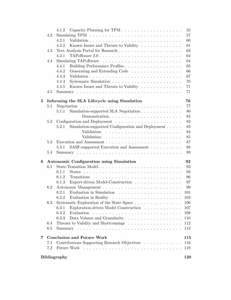
1 Introduction 11.1 Research Problem and Objectives . . . . . . . . . . . . . . . . . . . . 11.2 Achieving the Research Objectives . . . . . . . . . . . . . . . . . . . 31.3 Organization of this Dissertation . . . . . . . . . . . . . . . . . . . . 4
2 Background and Related Work 62.1 Services Overview . . . . . . . . . . . . . . . . . . . . . . . . . . . . 7
2.1.1 Service Level Agreements . . . . . . . . . . . . . . . . . . . . 82.2 Characteristics of Simulation Frameworks . . . . . . . . . . . . . . . 102.3 Simulation Frameworks for SOAs . . . . . . . . . . . . . . . . . . . . 13
2.3.1 SOAD and DEVS . . . . . . . . . . . . . . . . . . . . . . . . 152.3.2 DDSOS . . . . . . . . . . . . . . . . . . . . . . . . . . . . . . 162.3.3 MaramaMTE . . . . . . . . . . . . . . . . . . . . . . . . . . . 162.3.4 SOPM . . . . . . . . . . . . . . . . . . . . . . . . . . . . . . . 172.3.5 Narayanan (DAML) . . . . . . . . . . . . . . . . . . . . . . . 182.3.6 Commercial Solutions . . . . . . . . . . . . . . . . . . . . . . 192.3.7 Discussion and Comparison . . . . . . . . . . . . . . . . . . . 20
2.4 Value, Quality, and Cost . . . . . . . . . . . . . . . . . . . . . . . . . 242.4.1 Web Services as Products . . . . . . . . . . . . . . . . . . . . 252.4.2 Propositions on Value . . . . . . . . . . . . . . . . . . . . . . 26
2.5 Capacity Planning and Configuration Management . . . . . . . . . . 292.6 Autonomic Computing: Self Management . . . . . . . . . . . . . . . 302.7 Summary . . . . . . . . . . . . . . . . . . . . . . . . . . . . . . . . . 33
3 Services-Aware Simulation Framework 353.1 Simulation Engine . . . . . . . . . . . . . . . . . . . . . . . . . . . . 363.2 wsdl2sim . . . . . . . . . . . . . . . . . . . . . . . . . . . . . . . . . . 393.3 JIMMIE: Systematic Simulation Configuration . . . . . . . . . . . . 433.4 Metrics Engine . . . . . . . . . . . . . . . . . . . . . . . . . . . . . . 443.5 Emulation Extension . . . . . . . . . . . . . . . . . . . . . . . . . . . 453.6 Service Testing Modules Extension . . . . . . . . . . . . . . . . . . . 463.7 Using Simulation-driven Methodologies . . . . . . . . . . . . . . . . . 483.8 Known Issues and Threats to Validity . . . . . . . . . . . . . . . . . 493.9 Summary . . . . . . . . . . . . . . . . . . . . . . . . . . . . . . . . . 50
4 Simulating Service Oriented Applications 514.1 Tivoli Provisioning Manager . . . . . . . . . . . . . . . . . . . . . . . 52
4.1.1 Executing Jobs using the SDI . . . . . . . . . . . . . . . . . . 54
4.1.2 Capacity Planning for TPM . . . . . . . . . . . . . . . . . . . 554.2 Simulating TPM . . . . . . . . . . . . . . . . . . . . . . . . . . . . . 57
4.2.1 Validation . . . . . . . . . . . . . . . . . . . . . . . . . . . . . 604.2.2 Known Issues and Threats to Validity . . . . . . . . . . . . . 61
4.3 Text Analysis Portal for Research . . . . . . . . . . . . . . . . . . . . 634.3.1 TAPoRware 2.0 . . . . . . . . . . . . . . . . . . . . . . . . . . 64
4.4 Simulating TAPoRware . . . . . . . . . . . . . . . . . . . . . . . . . 644.4.1 Building Performance Profiles . . . . . . . . . . . . . . . . . . 654.4.2 Generating and Extending Code . . . . . . . . . . . . . . . . 664.4.3 Validation . . . . . . . . . . . . . . . . . . . . . . . . . . . . . 674.4.4 Systematic Simulation . . . . . . . . . . . . . . . . . . . . . . 704.4.5 Known Issues and Threats to Validity . . . . . . . . . . . . . 71
4.5 Summary . . . . . . . . . . . . . . . . . . . . . . . . . . . . . . . . . 71
5 Informing the SLA Lifecycle using Simulation 765.1 Negotiation . . . . . . . . . . . . . . . . . . . . . . . . . . . . . . . . 77
5.1.1 Simulation-supported SLA Negotiation . . . . . . . . . . . . . 80Demonstration. . . . . . . . . . . . . . . . . . . . . . . 82
5.2 Configuration and Deployment . . . . . . . . . . . . . . . . . . . . . 835.2.1 Simulation-supported Configuration and Deployment . . . . . 83
Validation: . . . . . . . . . . . . . . . . . . . . . . . . 84Validation: . . . . . . . . . . . . . . . . . . . . . . . . 85
5.3 Execution and Assessment . . . . . . . . . . . . . . . . . . . . . . . . 875.3.1 SASF-supported Execution and Assessment . . . . . . . . . . 88
5.4 Summary . . . . . . . . . . . . . . . . . . . . . . . . . . . . . . . . . 89
6 Autonomic Configuration using Simulation 926.1 State-Transition Model . . . . . . . . . . . . . . . . . . . . . . . . . . 93
6.1.1 States . . . . . . . . . . . . . . . . . . . . . . . . . . . . . . . 936.1.2 Transitions . . . . . . . . . . . . . . . . . . . . . . . . . . . . 966.1.3 Expert-driven Model-Construction . . . . . . . . . . . . . . . 97
6.2 Autonomic Management . . . . . . . . . . . . . . . . . . . . . . . . . 996.2.1 Evaluation in Simulation . . . . . . . . . . . . . . . . . . . . 1016.2.2 Evaluation in Reality . . . . . . . . . . . . . . . . . . . . . . 103
6.3 Systematic Exploration of the State Space . . . . . . . . . . . . . . . 1066.3.1 Exploration-driven Model Construction . . . . . . . . . . . . 1076.3.2 Evaluation . . . . . . . . . . . . . . . . . . . . . . . . . . . . 1086.3.3 Data Volume and Granularity . . . . . . . . . . . . . . . . . . 110
6.4 Threats to Validity and Shortcomings . . . . . . . . . . . . . . . . . 1126.5 Summary . . . . . . . . . . . . . . . . . . . . . . . . . . . . . . . . . 113
7 Conclusion and Future Work 1157.1 Contributions Supporting Research Objectives . . . . . . . . . . . . 1167.2 Future Work . . . . . . . . . . . . . . . . . . . . . . . . . . . . . . . 118
Bibliography 120
List of Figures
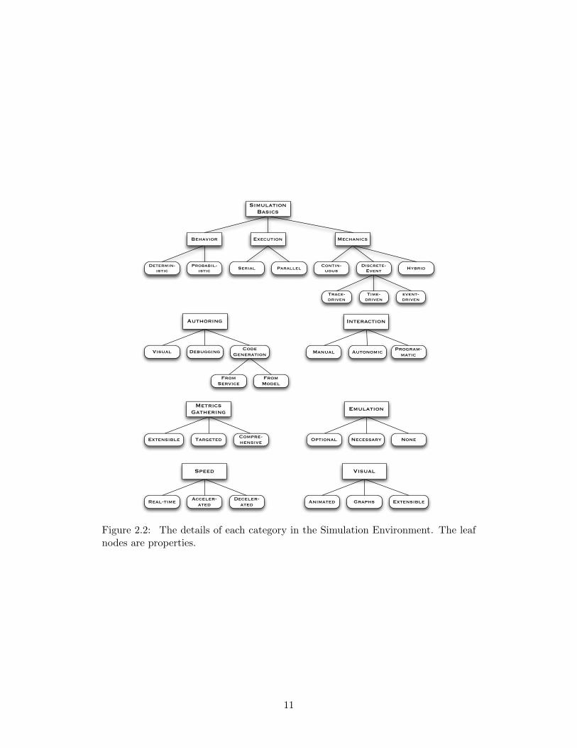
2.1 The overall Simulation Environment properties. . . . . . . . . . . . . 102.2 The details of each category in the Simulation Environment. The leaf
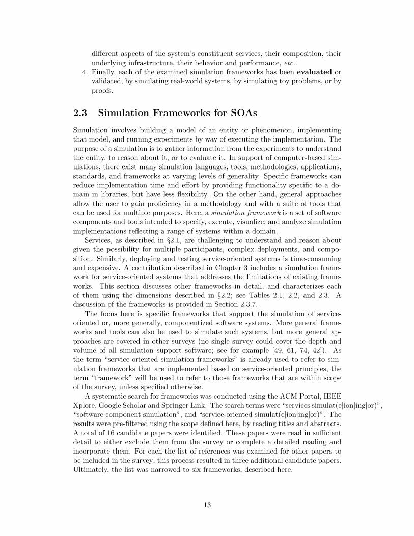
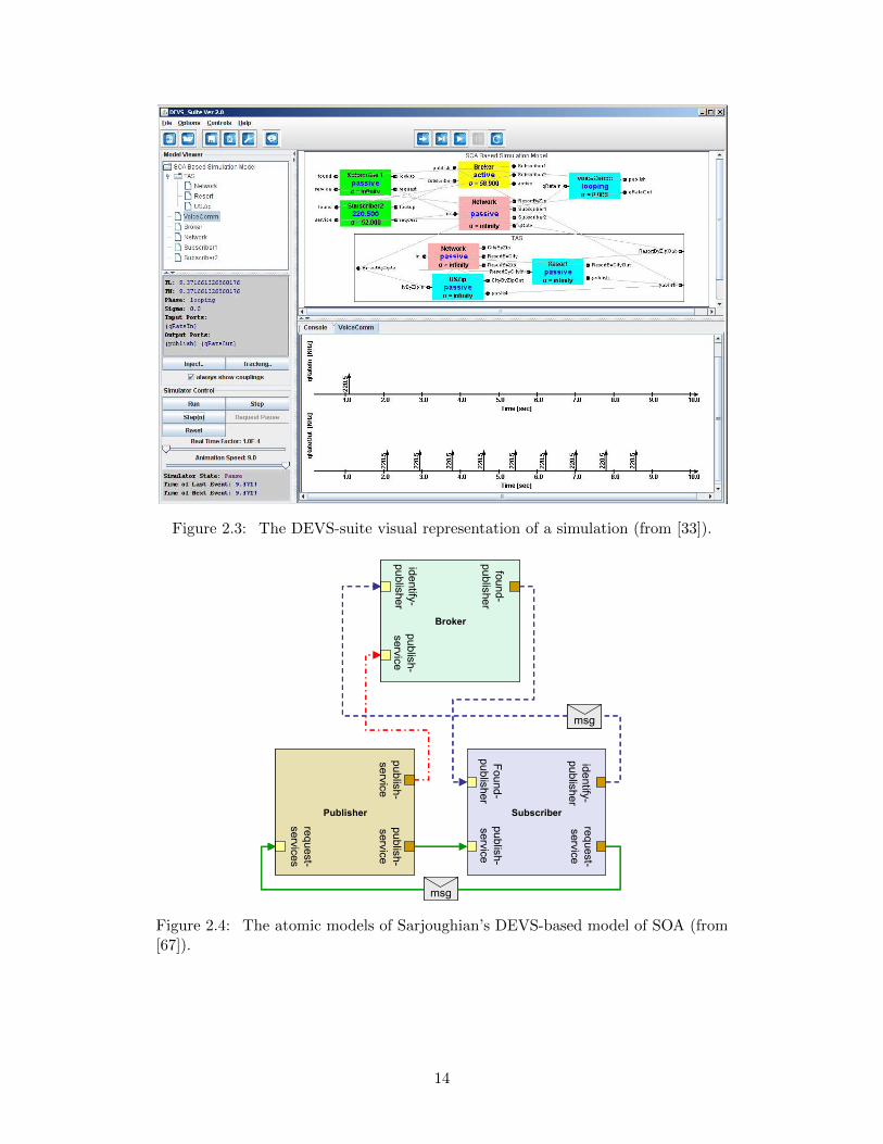
nodes are properties. . . . . . . . . . . . . . . . . . . . . . . . . . . . 112.3 The DEVS-suite visual representation of a simulation (from [33]). . . 142.4 The atomic models of Sarjoughian’s DEVS-based model of SOA (from
[67]). . . . . . . . . . . . . . . . . . . . . . . . . . . . . . . . . . . . . 142.5 Screenshot of the SOPM visual model building tool (from [7]). . . . 172.6 The KarmaSIM environment, showing the Congo example in execu-
tion (from [50]). . . . . . . . . . . . . . . . . . . . . . . . . . . . . . 182.7 SoapUI, shown exploring the WSDL for Amazon EC2: a generated
request and an Amazon response, a running mock service, and a loadtesting applet. . . . . . . . . . . . . . . . . . . . . . . . . . . . . . . 19
2.8 Limitations of the distinguishing characteristics of services, from [78]. 272.9 The Model, Analyze, Plan and Execute model of autonomic comput-
ing, from [26]. . . . . . . . . . . . . . . . . . . . . . . . . . . . . . . . 31
3.1 The primary components and extensions of SASF. . . . . . . . . . . 363.2 A class diagram of selected extensible service objects. . . . . . . . . 373.3 A class diagram of selected message objects. . . . . . . . . . . . . . . 393.4 A sample two-server, four-operation topology descriptor. The simu-
lation using this topology is described in §4.4. . . . . . . . . . . . . . 393.5 The high-level structure of a WSDL document. Each component
can be characterized as a more abstract description or as being moreabout implementation. . . . . . . . . . . . . . . . . . . . . . . . . . . 40
3.6 A portion of the <types> section of a WSDL document and the codeproduced. . . . . . . . . . . . . . . . . . . . . . . . . . . . . . . . . . 41
3.7 A sample JIML document, which increments by 100 the height at-tribute of the <location> tag that has id “main” for each of the 1000experiments, add an attribute width to the same element, add a newelement hello, and remove the element useless with id 123. . . . . 43
3.8 A class diagram of selected metrics objects. . . . . . . . . . . . . . . 453.9 The visualization metrics listener displaying two of the metrics being
captured by a simulation. . . . . . . . . . . . . . . . . . . . . . . . . 463.10 A custom metrics listener and the playback control. . . . . . . . . . 473.11 A class diagram of selected Service Testing Module (STM) components. 48
4.1 A conceptual model of the SDI in an example scenario. . . . . . . . . 534.2 A high-level sequence diagram of job publishing. . . . . . . . . . . . 544.3 A high-level sequence diagram of job distribution. . . . . . . . . . . . 55
4.4 Current process plus the capacity planning tool. . . . . . . . . . . . 564.5 The class hierarchy implemented for the simulation. . . . . . . . . . 574.6 The topology XML document used to configure the simulated networks. 584.7 The document describing the TPM infrastructure. . . . . . . . . . . 584.8 Source lines of code for the TPMsim-specific code and the framework. 604.9 Time required to send a 10M file to endpoints, simulated vs. emulated. 604.10 Custom visualizations in the TPM simulation dashboard. . . . . . . 624.11 The modification tool for modifying parameters of request-generation
in real time. . . . . . . . . . . . . . . . . . . . . . . . . . . . . . . . . 674.12 The proportion of hand-written code versus code provided by a library
or automatically-generated. . . . . . . . . . . . . . . . . . . . . . . . 684.13 The proportion of hand-written code versus automatically-generated,
excluding framework code. . . . . . . . . . . . . . . . . . . . . . . . . 684.14 Normalized distributions of service response times to single concur-
rent requests, comparing reality to the theoretic model (linear regres-sion) and the implemented model (simulation). . . . . . . . . . . . . 69
4.15 The total time required for the real service and the simulated serviceto respond to all 50 requests for varying input sizes. . . . . . . . . . 70
4.16 The JIML file describing what parameters to modify for a series ofexperiments. . . . . . . . . . . . . . . . . . . . . . . . . . . . . . . . 73
4.17 The data produced by JIMMIE; the relative size of the request isshown by the size of the point. The overlap between service concur-rency of 1 and 2 shows that this factor doesn’t affect the results. Theaverage response time increases as the request load on the serviceincreases. . . . . . . . . . . . . . . . . . . . . . . . . . . . . . . . . . 74
5.1 The traditional view of an SLA lifecycle (from [24]): a linear run fromnegotiation to termination. . . . . . . . . . . . . . . . . . . . . . . . 77
5.2 The lifecycle of an SLA: negotiated, implemented, assessed, then re-negotiated or terminated. . . . . . . . . . . . . . . . . . . . . . . . . 77
5.3 Diagram of the current state of SLAs: providers implement SLAsby converting them into SLMs and ultimately system configurations.Consumers interact with an SLA directly, but there is no informationon how it maps to customer satisfaction. . . . . . . . . . . . . . . . . 78
5.4 Expanding the top-level goal of “satisfaction” to one level is feasible;the direct link between SLA terms and satisfaction is less clear. . . . 79
5.5 A visualization of configurations’ Average Response Time versus theiroverall time to process. . . . . . . . . . . . . . . . . . . . . . . . . . . 81
5.6 Simulation-generated answers for how the List Words operation han-dles varying levels of concurrency for varying numbers of proces-sors/cores. . . . . . . . . . . . . . . . . . . . . . . . . . . . . . . . . . 85
5.7 Real-world answers for how the List Words operation handles varyinglevels of concurrency for varying numbers of processors/cores. . . . . 86
5.8 Distribution question answering results. . . . . . . . . . . . . . . . . 875.9 IBM Netcool Service Quality Manager (from [27]Distribution ques-
tion answering results. . . . . . . . . . . . . . . . . . . . . . . . . . . 885.10 The actual graphs displayed in the Metrics Dashboard, unifying real-
world metrics with metrics created or measured by the simulation. . 91
6.1 A hypothetical fragment of a state diagram; states can be satisfactory,unsatisfactory, or boundary; transitions occur when the load changesor the configuration changes. . . . . . . . . . . . . . . . . . . . . . . 96
6.2 The states identified in three simulation traces; a permissive SLAensures they are all S-states, each transition is annotated with itsprobability. . . . . . . . . . . . . . . . . . . . . . . . . . . . . . . . . 98
6.3 The performance / cost trade-offs for the linearly increasing data setin simulation. . . . . . . . . . . . . . . . . . . . . . . . . . . . . . . . 100
6.4 The performance / cost trade-offs for the variable data set in simulation.1026.5 Directed graph showing the states and transitions from a 3-hour ex-
ecution of the simulation. Colors show the SUB metric; color andthickness of edges show frequency of transition. . . . . . . . . . . . . 104
6.6 The components of the real-world testing architecture. . . . . . . . . 1056.7 The performance / cost trade-offs for the variable data set as tested
in a real cloud. . . . . . . . . . . . . . . . . . . . . . . . . . . . . . . 1066.8 The number of servers over time as configured by the autonomic
manager in the real-world testing. . . . . . . . . . . . . . . . . . . . 1066.9 The high-level architecture of the systematic exploration. . . . . . . 1076.10 A sample actions XML document, naming actions to be taken when
the given states are encountered. . . . . . . . . . . . . . . . . . . . . 1096.11 Number of simulations in each generation (log scale). . . . . . . . . . 1096.12 Average number of simulations enqueued per simulation for each gen-
eration. . . . . . . . . . . . . . . . . . . . . . . . . . . . . . . . . . . 1106.13 The number of experiments (y, log scale) that enqueued the given
number of experiments (x). . . . . . . . . . . . . . . . . . . . . . . . 1116.14 The performance / cost trade-offs for the test configurations. . . . . 1116.15 The performance / cost trade-offs for the test configurations with
various granularity. . . . . . . . . . . . . . . . . . . . . . . . . . . . . 112
List of Tables
2.1 Goals of various simulation frameworks. . . . . . . . . . . . . . . . . 202.2 Simulation environment properties. . . . . . . . . . . . . . . . . . . . 212.3 The modeling, coupling, and evaluation properties. . . . . . . . . . . 222.4 Comparing traditional definitions of services to Web Services. . . . . 26
3.1 Mapping from standard XML simple data types to Java data types. 40
4.1 Configuration parameters. . . . . . . . . . . . . . . . . . . . . . . . . 614.2 TAPoR operations . . . . . . . . . . . . . . . . . . . . . . . . . . . . 634.3 List Words operation response times for input of varying size submit-
ted one request at a time. . . . . . . . . . . . . . . . . . . . . . . . . 664.4 Mean Absolute Error when comparing the linear regression prediction
for the List Words operation to the real-world operation. . . . . . . . 674.5 List Words operation response times and total processing time for
configurations that vary in request concurrency, service processingconcurrency, and size. . . . . . . . . . . . . . . . . . . . . . . . . . . 75
5.1 Some of the meta data about the expected requests that informedthe manual configuration. . . . . . . . . . . . . . . . . . . . . . . . . 87
6.1 The elements of a snapshot descriptor for TAPoRsim. . . . . . . . . 946.2 Cost and performance metrics (and improvements) for 6 configura-
tions and the linearly increasing data set in simulation. . . . . . . . . 1016.3 Cost and performance metrics (and improvements) for 6 configura-
tions and the variable data set in simulation. . . . . . . . . . . . . . 1026.4 Cost and performance metrics (and improvements) for 6 configura-
tions and the variable data set as tested in a real cloud. . . . . . . . 1036.5 The changes to state space and coverage with changing granularity. . 112
List of Acronyms
ACUS Autonomic Configuration using Simulation
ANOVA Analysis of Variance
API Application Programming Interface
AWS Amazon Web Services
BPEL Business Process Execution Language
BPMN Business Process Modelling Notation
CDS Content Delivery Service
CDS-M Content Delivery Service Manager
CDS-D Content Delivery Service Depot
CGI Common Gateway Interface
DAML DARPA agent markup language
DARPA Defense Advanced Research Projects Agency
DDSOS Dynamic Distributed Service-Oriented Simulation Framework
DEVS Discrete Event System Specification
DEVSJAVA Java implementation of Discrete Event System Specification
DFS Depth First Search
DMS Device Manager Service
FIFO First-in, First-out [queue]
GB Gigabyte
GHz Gigahertz
GUI Graphical User Interface
HTML Hypertext Markup Language
IDDFS Iterative-deepening Depth First Search
IO Input/Output
IT Information Technology
JIML Jimmie Markup Language
JIMMIE Just Imagine Many Many Interesting Experiments
MAPE Model, Analyze, Plan, Execute
MB Megabyte
OASIS Organization for the Advancement of Structured InformationStandards
OS Quality of Service
OWL Web Ontology Language
PRISM A probabilistic model checker
PSML-S Process Specification and Modelling Language for Services
QoS Quality of Service
RATER Reliability, Assurance, Tangibles, Empathy, and Responsiveness
REST Representational State Transfer (e.g. HTTP)
SASF Services-aware Simulation Framework
SDI Software Distribution Infrastructure
SERVPERF A service quality assessment method
SERVQUAL A service quality assessment method
SLA Service Level Agreement
SLM Service Level Management
SLOC Source Lines of Code
SOA Service Oriented Architecture
SOAD SOA-compliant DEVS
SOAP Simple Object Access Protocol (no longer an acronym)
SOPM Service-Oriented Performance Modelling
SQL Standard Query Language
SSL Secure Sockets Layer
STM Service Testing Module
SUB Satisfactory, Unsatisfactory, Boundary state descriptors
TAPoR Text Analysis Portal for Research
TCA Tivoli Common Agent
TPM Tivoli Provisioning Manager
UI User Interface
UML Unified Modeling Language
URI Uniform Resource Identifier
WS Web Services
WSDL Web Services Description Language
XML eXtensible Markup Language
XSD XML Style Document
XSLT Extensible Stylesheet Language Transformations
Chapter 1
Introduction
Service-oriented architectures and flexible, scalable computing infrastructures promiseuseful functionality such as interoperability across organizations, software servicesystems that can be deployed and run quickly, managed infrastructure, and align-ment of business processes with technical implementations of those processes. Service-oriented architectures are loosely coupled, componentized, and standards-based.This composability, interoperability, and standardization enables re-use and theseamless replacement of one service with another offering the same interface. SOAis a potentially flexible architecture that enables interaction among multiple serviceproviders and service consumers, creation of complex functionality by composingseveral simpler components, and a network-driven infrastructure.
The current state of the art for providing this functionality is services-orientedarchitectures and cloud computing. Regardless of the ability of these specific tech-nologies to meet their promises, this functionality will continue to be sought.
This functionality introduces challenges inherent to complicated systems: thereare multiple organizations involved, the behavior of the system is difficult to pre-dict based solely on the behavior of the individual components, and technical deci-sions may be dictated by business decisions made without consideration of technicalchallenges. Generally speaking, flexibility leads to complexity in decision-making.Complexity cannot be removed from a closed system; it can only be moved fromone component or stage to another. By allowing organizations to integrate soft-ware systems, the complexity is transferred from information sharing to creatingand implementing the agreements that govern such interactions. The missing stepis hiding that complexity from non-technical decision makers by offering tools andmethodologies that simplify this process. A flexible computing infrastructure posesthe challenge of actually configuring and managing that infrastructure in the face ofchanging business requirements and technical abilities. Distributed, loosely-coupledsoftware systems solve interaction problems and can reduce development time, atthe cost of making configuring, deploying and testing the software system morecomplex.
1.1 Research Problem and Objectives
Research in configuration management has attempted to address the challenge ofconfiguring software of increasing complexity. The typical approach to configuring a
1
deployed software service system involves a trial-and-error reactive approach looselybased on a set of application-specific best practices. There is some expertise in thearea of configuring at the systems level - servers and networks - but application-levelconfiguration expertise is domain- or application-specific when it exists at all. Theresult is an expensive and time-consuming process of configuring a deployed service,or maintaining a sophisticated replica testing environment, or investing in an emu-lation environment to test possible configurations. In the case of a multiple-entityservice composition, such testing may be impossible or prohibitively expensive.
Another way to meet the configuration challenge is self-managing (autonomic)systems. A key challenge for such systems is producing a decision model - some-how translating raw metrics monitored from a service system into actions that re-configure the system (or, inaction). An approach more involved than simply makingchanges when a threshold is exceeded is desired; in particular, an approach that isable to make pro-active configuration changes to avoid thresholds completely. Thereis general distrust of many decision models because they are difficult to understand- the model is seen as a black-box oracle that produces re-configuration actions thatare difficult to understand.
Given that service providers have difficulty understanding and configuring theirown services, it may be surprising that service consumers are expected to partici-pate in establishing agreements specifying minimum performance standards for theservices they use. Research shows that consumers who are able to experience aproduct are better able to assess its quality and make decisions about cost versusquality trade-offs. Typically this can’t happen until a service is deployed - afterwhich changes are more expensive and more disruptive.
A solution that addresses each of these problems is to produce a simulated ver-sion of the target service system, then use simulation-generated data to assist inconfiguring services, to construct decision models for self-managing systems, and toinform and educate service providers and consumers. Unlike a pure analytic model,simulation can predict a narrative for a service system in a given scenario over time,making the results explainable and understandable. The current state of the art insimulating service-oriented systems is a) more focused on composition bottlenecksinstead of on the QoS attributes of each component of a service system, and b)less focused on tools to help communicate a plausible narrative (visualizations, met-rics generation, probabilistic models). Existing solutions also require substantialmodeling and/or development effort and expertise specific to the simulation tool.
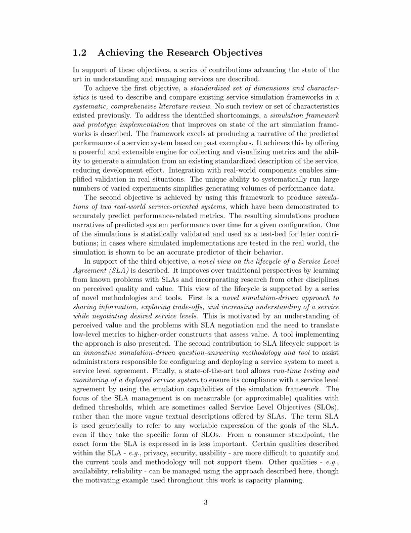
The aim of this dissertation is to absorb some of the complexity of configuring,deploying, governing, and managing service systems. The four research objectivesare as follows. First, to demonstrate that authoring a simulation of a service-orientedsystem need not be prohibitively difficult, and that such simulations can producea narrative that offers useful and realistic information about the predicted perfor-mance of a software system. Second, to use this approach to produce simulatedversions of real-world service systems using real performance data. Third, to showthat simulation-driven tools can be used to help manage the governance of softwaresystems throughout the cycle of negotiating standards for service performance, con-figuring the service to meet those standards, and evaluating and monitoring ongoingcompliance with those standards. Fourth, to demonstrate that a decision model gen-erated in simulation can be used to reason about a real-world software system, tothe point that such reasoning can be trusted to re-configure the service at run-time.
2
1.2 Achieving the Research Objectives
In support of these objectives, a series of contributions advancing the state of theart in understanding and managing services are described.
To achieve the first objective, a standardized set of dimensions and character-istics is used to describe and compare existing service simulation frameworks in asystematic, comprehensive literature review. No such review or set of characteristicsexisted previously. To address the identified shortcomings, a simulation frameworkand prototype implementation that improves on state of the art simulation frame-works is described. The framework excels at producing a narrative of the predictedperformance of a service system based on past exemplars. It achieves this by offeringa powerful and extensible engine for collecting and visualizing metrics and the abil-ity to generate a simulation from an existing standardized description of the service,reducing development effort. Integration with real-world components enables sim-plified validation in real situations. The unique ability to systematically run largenumbers of varied experiments simplifies generating volumes of performance data.
The second objective is achieved by using this framework to produce simula-tions of two real-world service-oriented systems, which have been demonstrated toaccurately predict performance-related metrics. The resulting simulations producenarratives of predicted system performance over time for a given configuration. Oneof the simulations is statistically validated and used as a test-bed for later contri-butions; in cases where simulated implementations are tested in the real world, thesimulation is shown to be an accurate predictor of their behavior.
In support of the third objective, a novel view on the lifecycle of a Service LevelAgreement (SLA) is described. It improves over traditional perspectives by learningfrom known problems with SLAs and incorporating research from other disciplineson perceived quality and value. This view of the lifecycle is supported by a seriesof novel methodologies and tools. First is a novel simulation-driven approach tosharing information, exploring trade-offs, and increasing understanding of a servicewhile negotiating desired service levels. This is motivated by an understanding ofperceived value and the problems with SLA negotiation and the need to translatelow-level metrics to higher-order constructs that assess value. A tool implementingthe approach is also presented. The second contribution to SLA lifecycle support isan innovative simulation-driven question-answering methodology and tool to assistadministrators responsible for configuring and deploying a service system to meet aservice level agreement. Finally, a state-of-the-art tool allows run-time testing andmonitoring of a deployed service system to ensure its compliance with a service levelagreement by using the emulation capabilities of the simulation framework. Thefocus of the SLA management is on measurable (or approximable) qualities withdefined thresholds, which are sometimes called Service Level Objectives (SLOs),rather than the more vague textual descriptions offered by SLAs. The term SLAis used generically to refer to any workable expression of the goals of the SLA,even if they take the specific form of SLOs. From a consumer standpoint, theexact form the SLA is expressed in is less important. Certain qualities describedwithin the SLA - e.g., privacy, security, usability - are more difficult to quantify andthe current tools and methodology will not support them. Other qualities - e.g.,availability, reliability - can be managed using the approach described here, thoughthe motivating example used throughout this work is capacity planning.
3
The fourth objective is achieved through an abstract decision model in the formof a state-transition model, constructed from simulation-generated data, useful foridentifying the state of an application and predicting future states. No existing deci-sion model generates a state-transition model from simulated data. A novel methodfor creating a self-managing software system is described, using the decision modelto make configuration and re-configuration decisions based on predicted futures.This is implemented and tested both in simulation and by using the self-manager tomake configuration changes in a real-world cloud computing environment. Finally,a novel approach (and implementation) systematically explores the state space of anapplication to construct a decision model automatically. This leads to an assessmentof what level of granularity offers the best abstraction of continuous data to producethe best translation between simulated environments and the real world.
1.3 Organization of this Dissertation
The existing state of the art is described in Chapter 2, including a background onservices; a comprehensive literature review of simulation support for service orientedsoftware; an introduction to value-related concepts like perceived value, perceivedquality, and perceived cost; and current research in capacity planning and configu-ration management and self-managing software. A novel contribution is provided inthe form of a set of characteristics useful for characterizing and comparing simulationframeworks for service-oriented systems (§2.2).
Chapter 3 introduces the Services-Aware Simulation Framework (SASF), a novelcontribution designed to create a virtual model of a service oriented system. SASFimproves on existing solutions by offering automatic generation of simulations fromexisting data about the service, a powerful approach to recording & visualizingsimulation-generated metrics, support for integrating with real-world components,and an extensible library of common service tasks. SASF uniquely offers accuratereplication of performance characteristics of services, an API and a user interfacefor interacting with a running simulation, and an innovative language and tool tosystematically modify simulation configuration files and execute simulations.
In Chapter 4, SASF is used to simulate two service systems. The first, a propri-etary enterprise-level system that includes SOA-based interfaces, is used to demon-strate simulations at a higher level of abstraction with less library support. Thesimulation models a distributed architecture used to publish files to thousands ofremote endpoints. It is shown that the simulated version produces results compara-ble to the real-world system (§4.1 and §4.2). The second is a text-analysis tool thatprovides a public web services interfaces. It is used to demonstrate automaticallygenerating a simulation with a one-to-one mapping between simulated componentsand real-world components (§4.3 and §4.4). Its CPU-bound operations are com-plex and interesting operations, but the relatively small number of these operationsmake it more manageable as a case study. This simulation, called TAPoRsim, is usedas a platform for demonstrating simulation-driven methodologies in the remainingchapters.
Chapter 5 is organized around the first contribution, a novel formulation of thelife cycle of a Service Level Agreement (SLA). These documents govern the inter-actions between a service provider and a service consumer; they are cyclic because
4

they should be re-negotiated and re-evaluated periodically as business and technicalneeds change. The second contribution draws on an understanding of perceivedvalue to describe the problems with SLA negotiation and identify a simulation-driven approach to sharing information and increasing understanding of the service(§5.1). The third describes a simulation-driven approach to answering specific ques-tions posed by those responsible for configuring and deploying a service system thatcomplies with the SLA (§5.2). The fourth contribution describes a SASF-supportedapproach to testing and monitoring a deployed service system (§5.3). Each contri-bution is implemented and demonstrated using TAPoRsim.
A novel method for creating a self-managing software service system is describedin Chapter 6. Configuration management is a complex task, even for experiencedsystem administrators, which makes self-managing systems a desirable contribution.The first contribution is an abstract decision model in the form of a state-transitionmodel, useful for identifying the state of an application and predicting future states(§6.1). A second contribution uses this model as the basis for self-management fea-tures that use predicted futures to make decisions on configuration changes (§6.2).This is validated both in simulation and by using the self-manager to make config-uration changes in a real-world cloud computing environment. Third, an approachand an implementation to systematically explore the state space of an applicationto support constructing a decision model (§6.3). Finally, the granularity requiredfor such a decision model to be effective is described and tested empirically.
The contributions are summarized and future work is presented in Chapter 7.
5
Chapter 2
Background and Related Work
Chapter Contents
2.1 Services Overview . . . . . . . . . . 7
2.1.1 Service Level Agreements . . . 8
2.2 Characteristics of SimulationFrameworks . . . . . . . . . . . . . . 10
2.3 Simulation Frameworks for SOAs . . 13
2.3.1 SOAD and DEVS . . . . . . . . 15
2.3.2 DDSOS . . . . . . . . . . . . . 16
2.3.3 MaramaMTE . . . . . . . . . . 16
2.3.4 SOPM . . . . . . . . . . . . . . 17
2.3.5 Narayanan (DAML) . . . . . . 18
2.3.6 Commercial Solutions . . . . . 19
2.3.7 Discussion and Comparison . . 20
2.4 Value, Quality, and Cost . . . . . . . 24
2.4.1 Web Services as Products . . . 25
2.4.2 Propositions on Value . . . . . 26
2.5 Capacity Planning and Configura-tion Management . . . . . . . . . . . 29
2.6 Autonomic Computing: Self Man-agement . . . . . . . . . . . . . . . . 30
2.7 Summary . . . . . . . . . . . . . . . 33
This chapter introduces background,terminology, and the current state ofthe art. Given the breadth in the areastouched by the contributions describedin this work, the various subsectionscover a diverse range of topics, rangingfrom industry standards to simulationto autonomic computing to marketingliterature.
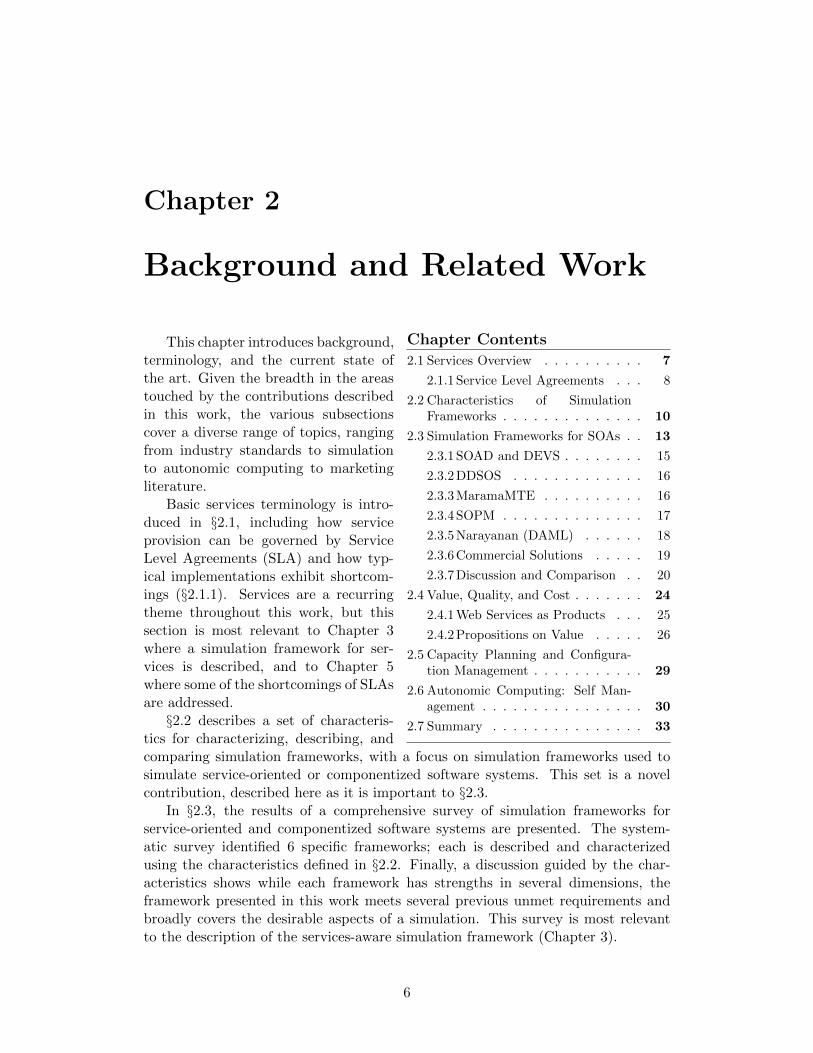
Basic services terminology is intro-duced in §2.1, including how serviceprovision can be governed by ServiceLevel Agreements (SLA) and how typ-ical implementations exhibit shortcom-ings (§2.1.1). Services are a recurringtheme throughout this work, but thissection is most relevant to Chapter 3where a simulation framework for ser-vices is described, and to Chapter 5where some of the shortcomings of SLAsare addressed.§2.2 describes a set of characteris-
tics for characterizing, describing, andcomparing simulation frameworks, with a focus on simulation frameworks used tosimulate service-oriented or componentized software systems. This set is a novelcontribution, described here as it is important to §2.3.
In §2.3, the results of a comprehensive survey of simulation frameworks forservice-oriented and componentized software systems are presented. The system-atic survey identified 6 specific frameworks; each is described and characterizedusing the characteristics defined in §2.2. Finally, a discussion guided by the char-acteristics shows while each framework has strengths in several dimensions, theframework presented in this work meets several previous unmet requirements andbroadly covers the desirable aspects of a simulation. This survey is most relevantto the description of the services-aware simulation framework (Chapter 3).
6
An introduction to concepts like perceived value, perceived cost, and perceivedquality follows in §2.4. Included is a discussion on whether an implementation ofa service-oriented architecture should rightly be considered a product or a service(§2.4.1). A survey of marketing literature reveals how individuals evaluate value andservice quality when making purchasing decisions. This background is important tothe discussion of an SLA creation methodology in §5.1 and §5.1.1.
Selected state-of-the-art work on configuration management and capacity plan-ning is presented in §2.5. Provisioning sufficient resources to meet expected demandis most relevant to the question-answering methodology contribution that is intendedto help system administrators translate customer non-functional requirements to aconfigured software system (§5.2.1).
Autonomic computing related work is reviewed in §2.6. The goal of an autonomicsystem is to be self-managing; the more specific focus is on self-configuring softwaresystems. The archetypical architecture is presented, and the areas advanced by thiswork are identified. This section is most relevant to the simulation-based autonomiccomputing methodology presented in Chapter 6.
2.1 Services Overview
Service-oriented Architecture (SOA) is a relatively new software architecture for-malization. It has been embraced by academic researchers and companies. It’sprimary defining characteristic is meeting needs with capabilities: broadly speak-ing, units of functionality are discovered and loosely-coupled to meet a need. Thebuilding blocks of a Service-oriented Architecture are services. In the context ofservice-oriented computing, a service is a mechanism for accessing a capability viaa well-defined interface [10].
While this definition is implementation-agnostic, a common software implemen-tation specification is Web Services (WS), which offers a well-defined interface toserver-side software and a suite of standards1. This narrows the definition to a net-work accessible endpoint that communications using XML standards. A Web serviceis “a software system designed to support interoperable machine-to-machine inter-action over a network. It has an interface described in a machine-processable format(specifically WSDL). Other systems interact with the Web service in a manner pre-scribed by its description using SOAP2-messages, typically conveyed using HTTPwith an XML serialization in conjunction with other Web-related standards” [20].
A binding describes how to move from a specification to implementation; it is an“association between an interface, a concrete protocol and a data format. A bindingspecifies the protocol and data format to be used in transmitting messages definedby the associated interface” [20].
An operation is an action supported by the service. A service is capable ofproviding at least one action and potentially more. For example, a car rental servicemight have two operations: searching for a car to rent, and booking a car to rent.
Another specific form of service is a RESTful service. Such services use HTTP
1These standards, sometimes called the WS-* standards, are agreed to by major corporations,freely available online, and will not be discussed at length here.
2SOAP is officially no longer an acronym, it is a term unto itself; the original meaning wasSimple Object Access Protocol.
7
without a SOAP message wrapper to transmit messages. The responses are usuallystill in a standardized form: XML or JSON are common. One school of thoughtconsiders RESTful services to be architecturally different, to be resource-orientedrather than service-oriented. The terms and language used throughout this docu-ment are those used for Web Services; this is done without loss of generality andwithout endorsing one type of service over the other. The implemented tools dohave dependencies based on WS technologies; including RESTful services is not amethodological question, but rather an implementation issue.
Services can be composed to provide more complex functionality. Composedservices can be managed by choreography (where the services are told how to worktogether, and possibly intermediaries are created to help the two communicate,but there is no central control) or orchestration (where a central controller guidesthe sequence of services and transforms data as needed). The specification of howservices are composed can use the Business Process Execution Language (BPEL),which “defines a model and a grammar for describing the behavior of a businessprocess based on interactions between the process and its partners” [29]. It isa script multiple partners can follow to ensure execution of their shared businessprocess.
Web services allows for multiple-entity compositions. While not part of theWS-* standards, Service Level Agreements (SLAs) can be used to govern theseinteractions. A service level agreement (SLA) is a contract between two partiespromising a certain level of service. The level of service expected can be technical(response time, CPU load) or non-technical (time to helpdesk problem resolution),but is typically measurable. There may be penalties for dropping below this levelof service.
2.1.1 Service Level Agreements
Service Level Agreements (SLAs) can be used to govern interactions between serviceproviders and service consumers. A service level agreement (SLA) is a contract be-tween two parties promising a certain level of service. The level of service expectedcan be technical (response time, CPU load) or non-technical (time to helpdesk prob-lem resolution), but is typically measurable. There may be penalties for droppingbelow this level of service. The items in a service level agreement are called ServiceLevel Objectives (SLOs).
One type of SLA is static and used for all customers, like those dictated byservice providers (e.g. Amazon EC2). One can be a customer or not; this is theextent of “customization” available. Metrics are recorded by the consumer and mustbe reported to and validated by the provider in order for the penalty clause of a 10%refund to take effect. The other type are individual and specific based on the needsof the consumer and capabilities of the provider, in which case they are negotiatedand include organization-specific guarantees. Typically these service providers havean SLA template which can be tailored to the needs of the customer. This tailoringcan happen in a series of meetings prior to beginning the service experience; there arealso methods for negotiating SLAs automatically at run-time (e.g. [65, 44, 85, 35]).
Services covered by SLAs typically have reporting requirements so both theprovider and consumer can compare actual performance to target performance.These reports are typically high-level; for example, “green” means a service level
8
objective was met, “red” means it was missed, and “yellow” means that there wastrouble meeting the objective.
Although SLAs are the current standard practice, they do not always ensurecustomer satisfaction. Blomberg [6] conducted a study of interactions between con-sumers and providers. She identified five problems with how SLAs were used inthose interactions, three of which are particularly relevant. A 2008 Forrester Re-search study [19] and a paper identifying SLA principles and best practices byFitsilis [18] support her conclusions and offer additional problems, as follows:
• Information is difficult to understand. A Forrester study [19] concluded mostSLAs are defined in technical terms not accessible to business users. Fit-silis [18] emphasizes the difficulty in mapping service levels from low-levelmeasurable information to higher-level meaningful information, reporting thatonly technical specialists understand SLAs. He also emphasizes the impor-tance of changing this: the first two best practices identified are “service leveldefinitions should be business-based, meaningful to the users...” and “servicelevel definitions should be easily defined and measurable”. The author alsorecognizes that “the ultimate measure of service-level performance is customerperception and satisfaction”, but that this end-user experience is difficult tomeasure.
• Satisfied SLA metrics don’t mean satisfied customers. The SLA reports areuseful in the first few months as the provider adjusts service delivery to ensurethe metrics are “green”. However, once the service delivery is satisfied, theyappear to become less important, and may not indicate customer satisfaction.A 2008 Forrester study [19] refers to “misalignment”, the distance betweenconsumer expectations and what the provider is trying to achieve. In pointingout that SLAs often aren’t actually agreements, the report claims “... at theend of a budget period, business managers can say ‘it was not good enough forme to do my business’, even if the IT service levels were met on a mathematicalbasis from the IT point of view.” They advocate for improved understandingof higher-level requirements. Fitsilis [18] reports that requirements are oftenpoorly specified and difficult to enforce.
• Information is hoarded. Providers are reluctant to provide unfettered, un-nuanced access to performance data. This sometimes extends from an honestdesire to provide meaningful interpreted performance data that has been an-alyzed and summarized for the client. A reasonable theory, though one asyet unsupported by evidence, is since SLAs are legally binding contracts, theprovider may hesitate to give clients access to information that could be usedto enforce penalty clauses if not properly “interpreted”.
• SLAs are not proactive enough. Clients remarked that they wanted morefrom their service providers: a proactive approach to help the client identifytheir needs and proactively meet them. As Blomberg points out, this requiresa broad sharing of information that may not always be possible or popular.It also requires technical staff to have the ability to elicit requirements frombusiness users, and these two groups may not be able to communicate on thesame level. Fitsili [18] remarks that by only penalizing performance below
9
Simulation Environment
Simulation Basics Authoring Interaction Metrics
Gathering Emulation Speed Visual
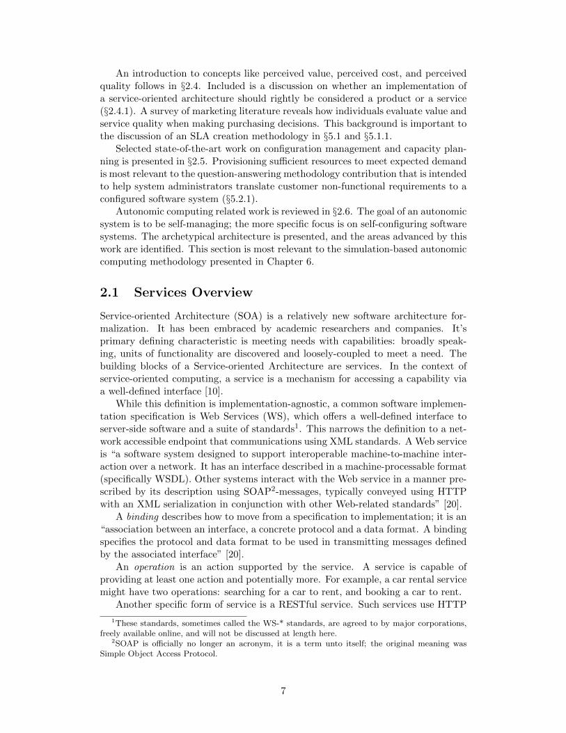
Figure 2.1: The overall Simulation Environment properties.
a minimum standard, providers are incentivized to strive for minimum levelsand no better.
• SLA obligations are not met. Forrester [19] reports that SLAs are unmet 75%of the time, and suggests the problem is that IT has moved from managingservers and networks to managing the applications (or at least the middleware)that runs on them.
Chapter 5 describes a set of contributions that improve on the challenges withSLAs above; respectively:
• Simulation-driven metrics visualization relates low-level metrics to higher-levelconstructs. The tools give consumers a chance to perceive quality in simulationbefore deploying to a real environment.
• The lifecycle proposed involves periodic re-evaluation of SLAs. Simulationallows customers to view a narrative of the expected performance of the servicebefore it is deployed. The configuration question answering tool helps serviceproviders align their configurations to service level obligations.
• By making information easier to understand, the incentive to hoard informa-tion is minimized. Substantial simulation-generated data can help satisfy thedesire for more information or prepare customers to receive larger volumes ofinformation from providers.
• The SLA negotiation tool enables an approach where the SLA is co-createdto maximize value to the client and help resolve trade-offs to the satisfactionof the customer.
• The question-answering tool helps translate SLA requirements to configurationvalues. The evaluation and monitoring tool simplifies periodic testing of theservice to ensure SLA obligations are being met. Additionally, Chapter 6describes an approach to automatically re-configure a service system to meetSLAs in rapidly changing environments.
2.2 Characteristics of Simulation Frameworks
To better classify simulation frameworks and compare them to the framework pro-posed in Chapter 3, the following set of simulation framework characteristics isdefined:
1. The first interesting characteristic feature of a simulation framework is itspurpose. Generally, a framework has one of two general objectives: (a) the
10
Interaction
Manual Autonomic Program-matic
Behavior
Determin-istic
Probabil-istic
Execution Mechanics
Contin-uous
Discrete-Event
Trace-driven
Time-driven
event-driven
HybridSerial Parallel
Simulation Basics
Authoring
Visual Debugging Code Generation
From Service
From Model
Metrics Gathering
Extensible Targeted Compre-hensive
Emulation
Optional Necessary None
Speed
Real-time Acceler-ated
Deceler-ated
Visual
Animated Graphs Extensible
Figure 2.2: The details of each category in the Simulation Environment. The leafnodes are properties.
11
examination of the system behavior in order to identify possibly undesirableinteractions in the composition of the system constituent services, and (b) theanalysis of the system performance.
2. The software design and functionalities of the simulation environment. Anoverview is in Figure 2.1 with the details of each branch in Figure 2.2.
• Basics: Based loosely on Sulistio et al. [73], this covers the fundamen-tals of the simulation. Continuous simulations are capable of trackinga system through any point of time, usually based on differential calcu-lus. Discrete-event simulations track a system based on specific momentsin time (time-based), as events occur (event-driven), or based on tracesfrom real-world applications. A deterministic simulation will produce thesame output for a given set of inputs every time it is run; stochastic orprobabilistic simulations use probability distributions and will produceoutput that varies based on the given distributions. Simulations can runin parallel, serially, or distributed (perhaps in a service-oriented architec-ture).
• Authoring: Typically a simulation is implemented using a language or byprogramming using an API or library. Some simulation frameworks aimto ease the process of simulating a system by offering authoring assistancesuch as visual simulation authoring, generating code automatically basedon the model or on the service itself (e.g. from WSDLs). Some simulationdevelopment environments offer tools intended to debug simulations.
• Interaction: Once a simulation is running, can the configuration, simu-lated entities, or other components be modified by a user (manual), bythe system itself (autonomic), or via an API (programmatic)?
• Metrics gathering: Real-world systems can be instrumented to producea variety of data. While simulations can be created to generate manytypes of data, often the focus is on a particular type of data (targeted).Others collect every metric generated by the simulation (comprehensive).Frameworks may be easily extensible to collect other metrics (for exam-ple, via an API).
• Visual Interface: Simulation results are usually reported in some textualrepresentation during the simulation run, or upon its completion. Inaddition, some frameworks include a visual component to visualize thesimulation or the metrics with either static images (default) or animatedimages. Also of interest is the ease with which the framework can beextended to improve, augment, or annotate the visualizing functions.
• Emulation: Some simulations offer the ability to interact with real-worldservices or entities. Others could require it as they cannot function ontheir own (for example, a simulation of a service broker might rely onreal-world services).
• Speed: Simulations can run faster than real time, in real time, or theo-retically slower than real time (perhaps due to computation required).
3. Different simulation frameworks adopt different modelling languages, ab-stract representations, or formalisms for specifying the systems under exami-nation. Each of these languages may make explicit (or alternatively, ignore)
12
different aspects of the system’s constituent services, their composition, theirunderlying infrastructure, their behavior and performance, etc..
4. Finally, each of the examined simulation frameworks has been evaluated orvalidated, by simulating real-world systems, by simulating toy problems, or byproofs.
2.3 Simulation Frameworks for SOAs
Simulation involves building a model of an entity or phenomenon, implementingthat model, and running experiments by way of executing the implementation. Thepurpose of a simulation is to gather information from the experiments to understandthe entity, to reason about it, or to evaluate it. In support of computer-based sim-ulations, there exist many simulation languages, tools, methodologies, applications,standards, and frameworks at varying levels of generality. Specific frameworks canreduce implementation time and effort by providing functionality specific to a do-main in libraries, but have less flexibility. On the other hand, general approachesallow the user to gain proficiency in a methodology and with a suite of tools thatcan be used for multiple purposes. Here, a simulation framework is a set of softwarecomponents and tools intended to specify, execute, visualize, and analyze simulationimplementations reflecting a range of systems within a domain.
Services, as described in §2.1, are challenging to understand and reason aboutgiven the possibility for multiple participants, complex deployments, and compo-sition. Similarly, deploying and testing service-oriented systems is time-consumingand expensive. A contribution described in Chapter 3 includes a simulation frame-work for service-oriented systems that addresses the limitations of existing frame-works. This section discusses other frameworks in detail, and characterizes eachof them using the dimensions described in §2.2; see Tables 2.1, 2.2, and 2.3. Adiscussion of the frameworks is provided in Section 2.3.7.
The focus here is specific frameworks that support the simulation of service-oriented or, more generally, componentized software systems. More general frame-works and tools can also be used to simulate such systems, but more general ap-proaches are covered in other surveys (no single survey could cover the depth andvolume of all simulation support software; see for example [49, 61, 74, 42]). Asthe term “service-oriented simulation frameworks” is already used to refer to sim-ulation frameworks that are implemented based on service-oriented principles, theterm “framework” will be used to refer to those frameworks that are within scopeof the survey, unless specified otherwise.
A systematic search for frameworks was conducted using the ACM Portal, IEEEXplore, Google Scholar and Springer Link. The search terms were “services simulat(e|ion|ing|or)”,“software component simulation”, and “service-oriented simulat(e|ion|ing|or)”. Theresults were pre-filtered using the scope defined here, by reading titles and abstracts.A total of 16 candidate papers were identified. These papers were read in sufficientdetail to either exclude them from the survey or complete a detailed reading andincorporate them. For each the list of references was examined for other papers tobe included in the survey; this process resulted in three additional candidate papers.Ultimately, the list was narrowed to six frameworks, described here.
13
4
3.1 Interface and Monitoring of Simulation Data
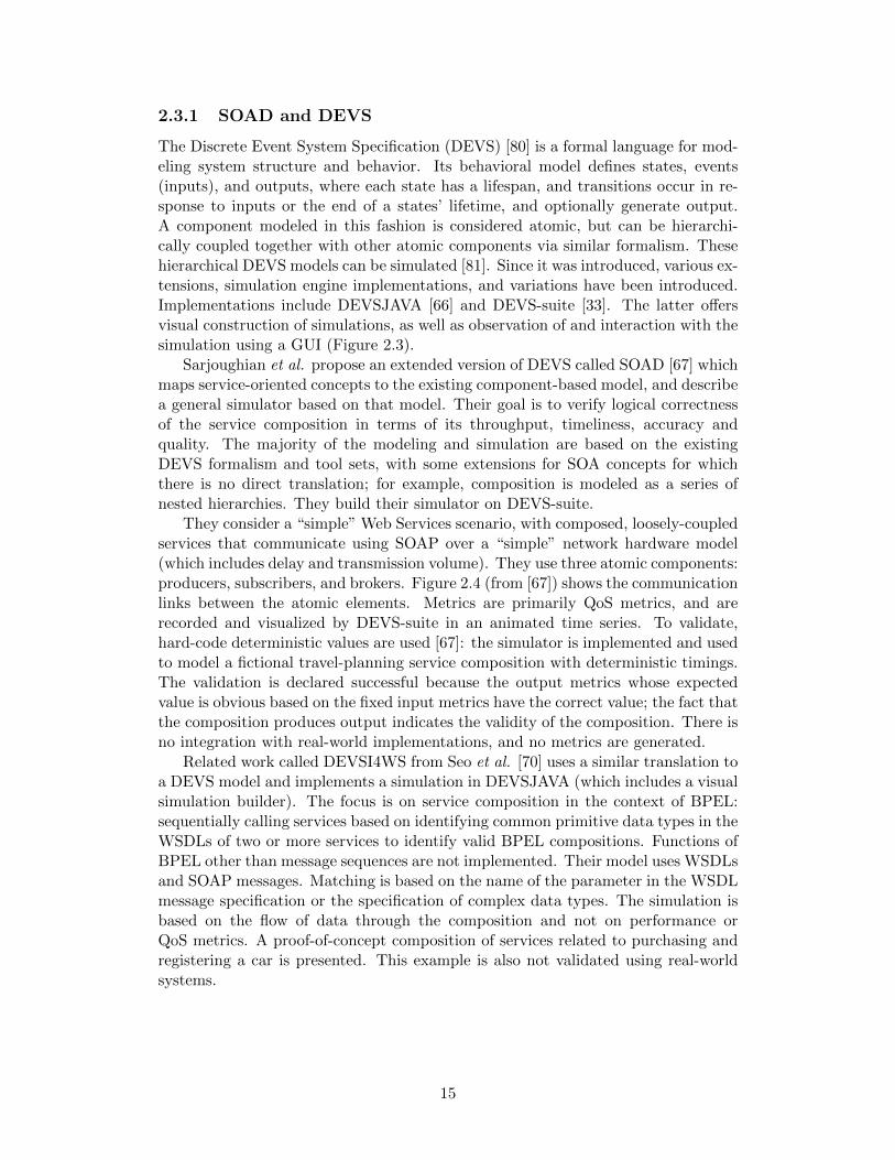
DEVS-Suite user interface consists of four parts: (1) Model Viewer at the top left corner, (2) Simulator Control at the bottom left corner, (3) simView at the top right hand corner, and (4) TimeView at the bottom right hand corner (see Figure 3). In order to make better use of available dis-play space, the Model Viewer and Simulator Control are combined to form a part which we call MVSC. A user, therefore, can choose to view any one of the TimeView, SimView, or MVSC parts within the DEVS-Suite interface since any two of the three parts can be hidden. A user may also view MVSC with either TimeView or SimView. Alter-natively, the user can hide the MVSC part and only view the TimeView and SimView while executing the model using the execution buttons provided in the menu bar.
Both block and tree views of hierarchical model com-ponents are available. It provides flexibility in that a user can select animation and/or tracking of simulation model
components as time trajectories. The tree view is used for choosing model components and deciding which input and output ports to monitor. For atomic models, pre-defined state variables and basic simulator variables can also be chosen and tracked. The block model is used for animation.
The dynamics of every atomic and coupled model can be individually displayed with TimeView. The semantics of the data generated by the Model module in DEVS-Suite is applied to the TimeView. Therefore, to display time-based state and input/output data, simulation time is used to syn-chronize generation of the time trajectories. Users have the flexibility to select animation and tracking view options for any number of atomic/coupled models. They can set the unit for data that is to be monitored as well as the time axis. The time increment, units, and the selection of data to be ob-served can be set as shown in Figure 4.
Figure 3: DEVS-Suite UI with Model Viewer, Simulator Control, simView, and TimeView
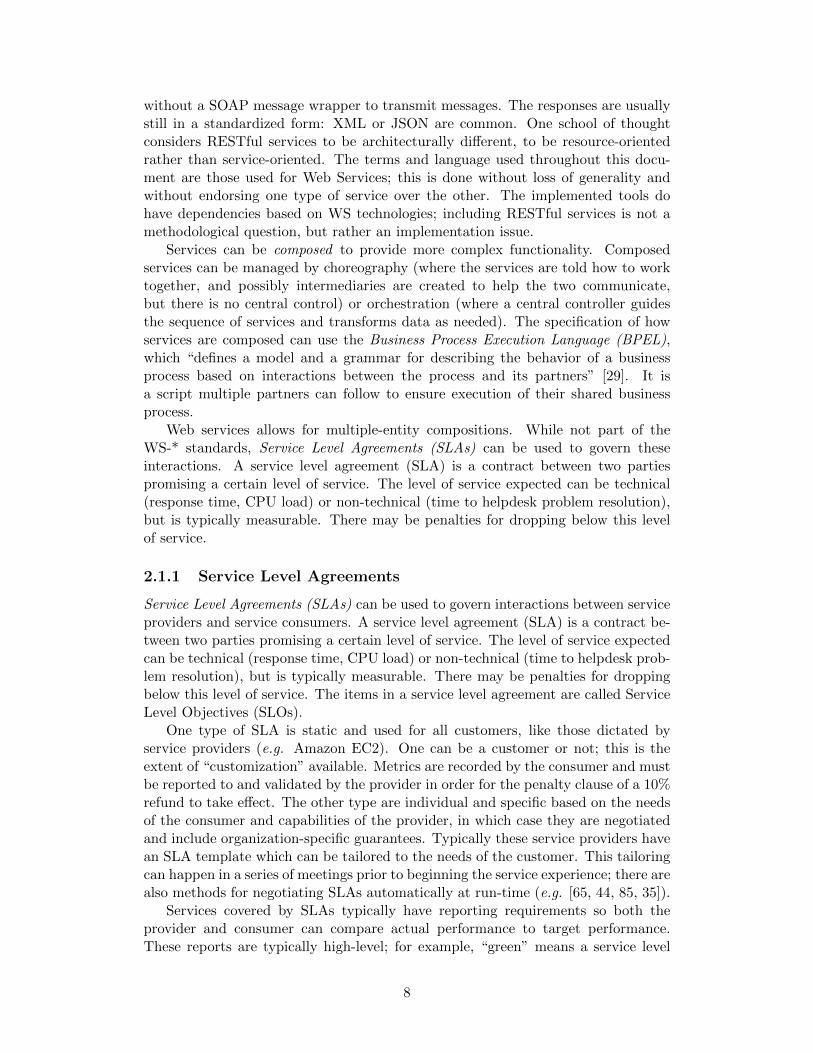
Figure 2.3: The DEVS-suite visual representation of a simulation (from [33]).
Sarjoughian, Kim, Ramaswamy, and Yau
5
software systems. Furthermore, the SOA is not the same as dynamic structure DEVS even though the structure of a coupled model can be modified during simulation.
5 SOAD SIMULATOR FRAMEWORK
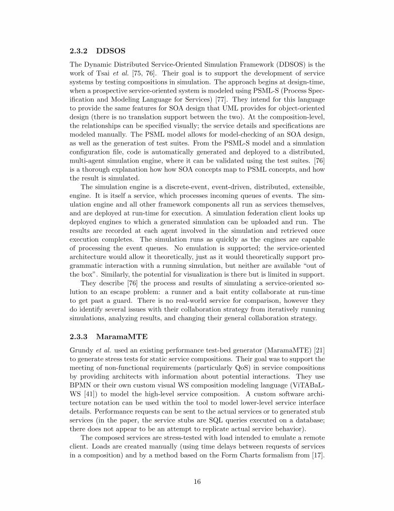
In the previous section, we described that there are basic similarities and differences between the SOA elements and those of DEVS. SOA framework has a higher level of ab-straction as compared with DEVS framework. The basic SOA model elements can be divided into two groups. First, services, service description, and messages represent the ‘static’ part of SOA. Second, communication agreement, messaging framework, and service registry and discovery represent the ‘dynamic’ part of the SOA. To create the SOAD Simulator (i.e., a generic SOA-complaint simula-tor), counterparts of the basic elements of SOA are needed. As shown in Table 1, we have defined a set of DEVS ele-ments that represent the static and dynamic aspects of the SOA. Three DEVS atomic models are proposed. Three of these have a one-to-one correspondence with the SOA ser-vices. The generic DEVSJAVA entity class is extended to represent SOA service description. Entity is also extended to represent SOA messages.
The publisher, subscriber, and broker services are the basic elements for both service-oriented software systems. The services can be synthesized to form primitive and composite service composition. Next, these two service compositions are described. A simple model of a network is used to complement the software aspect of SOA with the hardware aspect. It is defined as a link with finite capacity, transportation delay, and FIFO message queuing. This component is not a service – it models the medium through which services send and receive messages.
5.1 Primitive SOAD Models
The generic primitive service composition using DEVS atomic models (publisher, subscriber, and broker) is shown in Figure 2. Messages produced by a service and consumed by another are shown as envelops. As noted above, a mes-sage may contain a service description or other content consistent with a chosen messaging framework. For exam-ple, the message from the Broker to the Subscriber is a ser-vice description which contains an abstract definition (an interface for the operation names and their input and output messages) and a concrete definition (consisting of the bind-ing to physical transport protocol, address or endpoint, and service). Another message could be from the Publisher to the Subscriber where the result of the requested service (re-turned message from the Publisher). The implementation of these messages can be based on SOAP. In the basic SOA framework, the internal operations of atomic services and their interactions are deferred to specific standards and technologies (e.g., .NET (Lenz & Moeller 2003)).
Table 1: DEVS and SOA elements.
SOA Model Elements SOAD Model Elements
services (publisher, sub-scriber, broker)
atomic models (publisher, sub-scriber, broker)
service description entity (service-information) messages entity (service-lookup & ser-
vice-message) messaging framework ports & couplings service registry & discovery executive model service composition coupled models (primitive and
composite)
Publisher/Subscriber with Broker Coupled Model
Identify-publisher
Broker
identify-publisher
found-publisher
Publisher
request-services
publish-service
publish-service
Subscriber
Found-publisher
publish-service
identify-publisher
request-service
publish-service
request and response messages input port output portdata service messages publish messages
msg
msg
Publisher/Subscriber with Broker Coupled Model
Identify-publisher
Broker
identify-publisher
found-publisher
Publisher
request-services
publish-service
publish-service
Subscriber
Found-publisher
publish-service
identify-publisher
request-service
publish-service
request and response messages input port output portdata service messages publish messages
request and response messages input port output portdata service messages publish messages
msgmsg
msgmsg
Figure 2: SOAD primitive service composition
5.2 Composite SOAD Models
An essential capability for simulating service-based soft-ware systems is to support modeling of composite service composition. As shown in Figure 2, a composite service composition has publisher or subscriber service which it-self is a primitive service composition. Since broker ser-vice is required for both primitive and composite service composition, two cases can be considered – i.e., either a single broker service or multiple broker services are used. Both cases can be supported. Use of a single broker service is shown in Figure 3. To avoid cluttering Figure 3, the bro-kers shown in the Subscriber and Publisher services are the ones that are used for these brokers (this is shown with shaded background for the two brokers and their cou-plings). The three kinds of couplings provided in coupled DEVS models supports use of a single broker for the pri-mitive service compositions (i.e., Subscriber and Pub-lisher) and their composite (hierarchical) service composi-
849
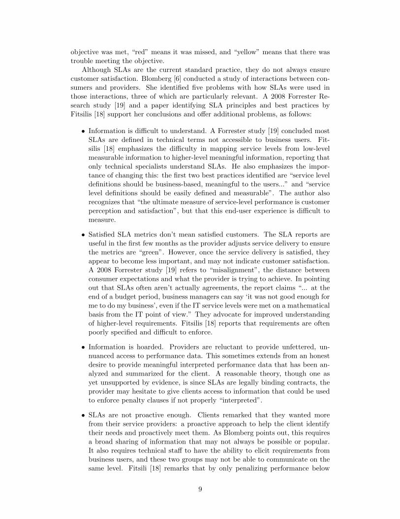
Figure 2.4: The atomic models of Sarjoughian’s DEVS-based model of SOA (from[67]).
14
2.3.1 SOAD and DEVS
The Discrete Event System Specification (DEVS) [80] is a formal language for mod-eling system structure and behavior. Its behavioral model defines states, events(inputs), and outputs, where each state has a lifespan, and transitions occur in re-sponse to inputs or the end of a states’ lifetime, and optionally generate output.A component modeled in this fashion is considered atomic, but can be hierarchi-cally coupled together with other atomic components via similar formalism. Thesehierarchical DEVS models can be simulated [81]. Since it was introduced, various ex-tensions, simulation engine implementations, and variations have been introduced.Implementations include DEVSJAVA [66] and DEVS-suite [33]. The latter offersvisual construction of simulations, as well as observation of and interaction with thesimulation using a GUI (Figure 2.3).
Sarjoughian et al. propose an extended version of DEVS called SOAD [67] whichmaps service-oriented concepts to the existing component-based model, and describea general simulator based on that model. Their goal is to verify logical correctnessof the service composition in terms of its throughput, timeliness, accuracy andquality. The majority of the modeling and simulation are based on the existingDEVS formalism and tool sets, with some extensions for SOA concepts for whichthere is no direct translation; for example, composition is modeled as a series ofnested hierarchies. They build their simulator on DEVS-suite.
They consider a “simple” Web Services scenario, with composed, loosely-coupledservices that communicate using SOAP over a “simple” network hardware model(which includes delay and transmission volume). They use three atomic components:producers, subscribers, and brokers. Figure 2.4 (from [67]) shows the communicationlinks between the atomic elements. Metrics are primarily QoS metrics, and arerecorded and visualized by DEVS-suite in an animated time series. To validate,hard-code deterministic values are used [67]: the simulator is implemented and usedto model a fictional travel-planning service composition with deterministic timings.The validation is declared successful because the output metrics whose expectedvalue is obvious based on the fixed input metrics have the correct value; the fact thatthe composition produces output indicates the validity of the composition. There isno integration with real-world implementations, and no metrics are generated.
Related work called DEVSI4WS from Seo et al. [70] uses a similar translation toa DEVS model and implements a simulation in DEVSJAVA (which includes a visualsimulation builder). The focus is on service composition in the context of BPEL:sequentially calling services based on identifying common primitive data types in theWSDLs of two or more services to identify valid BPEL compositions. Functions ofBPEL other than message sequences are not implemented. Their model uses WSDLsand SOAP messages. Matching is based on the name of the parameter in the WSDLmessage specification or the specification of complex data types. The simulation isbased on the flow of data through the composition and not on performance orQoS metrics. A proof-of-concept composition of services related to purchasing andregistering a car is presented. This example is also not validated using real-worldsystems.
15
2.3.2 DDSOS
The Dynamic Distributed Service-Oriented Simulation Framework (DDSOS) is thework of Tsai et al. [75, 76]. Their goal is to support the development of servicesystems by testing compositions in simulation. The approach begins at design-time,when a prospective service-oriented system is modeled using PSML-S (Process Spec-ification and Modeling Language for Services) [77]. They intend for this languageto provide the same features for SOA design that UML provides for object-orienteddesign (there is no translation support between the two). At the composition-level,the relationships can be specified visually; the service details and specifications aremodeled manually. The PSML model allows for model-checking of an SOA design,as well as the generation of test suites. From the PSML-S model and a simulationconfiguration file, code is automatically generated and deployed to a distributed,multi-agent simulation engine, where it can be validated using the test suites. [76]is a thorough explanation how how SOA concepts map to PSML concepts, and howthe result is simulated.
The simulation engine is a discrete-event, event-driven, distributed, extensible,engine. It is itself a service, which processes incoming queues of events. The sim-ulation engine and all other framework components all run as services themselves,and are deployed at run-time for execution. A simulation federation client looks updeployed engines to which a generated simulation can be uploaded and run. Theresults are recorded at each agent involved in the simulation and retrieved onceexecution completes. The simulation runs as quickly as the engines are capableof processing the event queues. No emulation is supported; the service-orientedarchitecture would allow it theoretically, just as it would theoretically support pro-grammatic interaction with a running simulation, but neither are available “out ofthe box”. Similarly, the potential for visualization is there but is limited in support.
They describe [76] the process and results of simulating a service-oriented so-lution to an escape problem: a runner and a bait entity collaborate at run-timeto get past a guard. There is no real-world service for comparison, however theydo identify several issues with their collaboration strategy from iteratively runningsimulations, analyzing results, and changing their general collaboration strategy.
2.3.3 MaramaMTE
Grundy et al. used an existing performance test-bed generator (MaramaMTE) [21]to generate stress tests for static service compositions. Their goal was to support themeeting of non-functional requirements (particularly QoS) in service compositionsby providing architects with information about potential interactions. They useBPMN or their own custom visual WS composition modeling language (ViTABaL-WS [41]) to model the high-level service composition. A custom software archi-tecture notation can be used within the tool to model lower-level service interfacedetails. Performance requests can be sent to the actual services or to generated stubservices (in the paper, the service stubs are SQL queries executed on a database;there does not appear to be an attempt to replicate actual service behavior).
The composed services are stress-tested with load intended to emulate a remoteclient. Loads are created manually (using time delays between requests of servicesin a composition) and by a method based on the Form Charts formalism from [17].
16
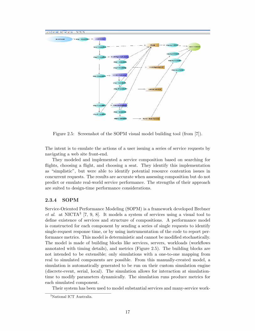
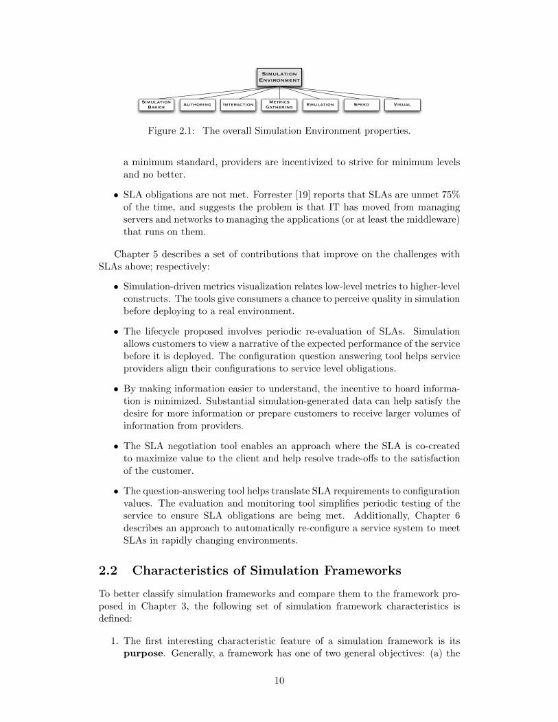
Figure 2.5: Screenshot of the SOPM visual model building tool (from [7]).
The intent is to emulate the actions of a user issuing a series of service requests bynavigating a web site front-end.
They modeled and implemented a service composition based on searching forflights, choosing a flight, and choosing a seat. They identify this implementationas “simplistic”, but were able to identify potential resource contention issues inconcurrent requests. The results are accurate when assessing composition but do notpredict or emulate real-world service performance. The strengths of their approachare suited to design-time performance considerations.
2.3.4 SOPM
Service-Oriented Performance Modeling (SOPM) is a framework developed Brebneret al. at NICTA3 [7, 9, 8]. It models a system of services using a visual tool todefine existence of services and structure of compositions. A performance modelis constructed for each component by sending a series of single requests to identifysingle-request response time, or by using instrumentation of the code to report per-formance metrics. This model is deterministic and cannot be modified stochastically.The model is made of building blocks like services, servers, workloads (workflowsannotated with timing details), and metrics (Figure 2.5). The building blocks arenot intended to be extensible; only simulations with a one-to-one mapping fromreal to simulated components are possible. From this manually-created model, asimulation is automatically generated to be run on their custom simulation engine(discrete-event, serial, local). The simulation allows for interaction at simulation-time to modify parameters dynamically. The simulation runs produce metrics foreach simulated component.
Their system has been used to model substantial services and many-service work-
3National ICT Australia.
17
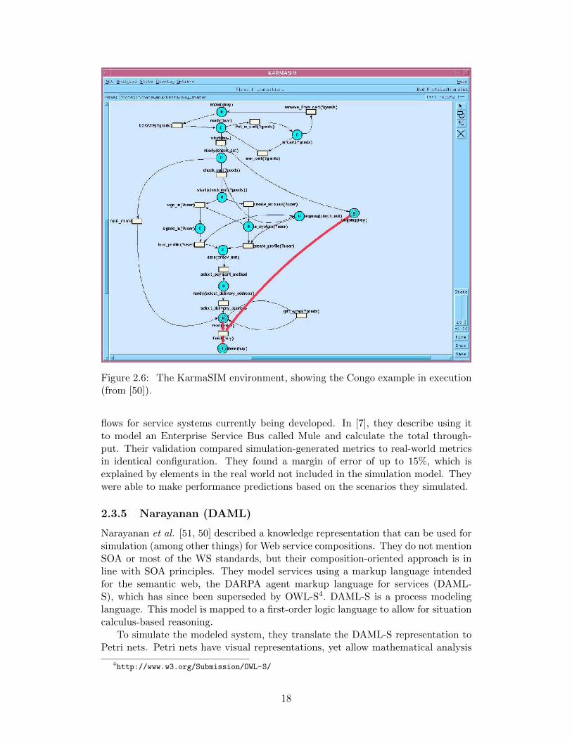
Figure 2.6: The KarmaSIM environment, showing the Congo example in execution(from [50]).
flows for service systems currently being developed. In [7], they describe using itto model an Enterprise Service Bus called Mule and calculate the total through-put. Their validation compared simulation-generated metrics to real-world metricsin identical configuration. They found a margin of error of up to 15%, which isexplained by elements in the real world not included in the simulation model. Theywere able to make performance predictions based on the scenarios they simulated.
2.3.5 Narayanan (DAML)
Narayanan et al. [51, 50] described a knowledge representation that can be used forsimulation (among other things) for Web service compositions. They do not mentionSOA or most of the WS standards, but their composition-oriented approach is inline with SOA principles. They model services using a markup language intendedfor the semantic web, the DARPA agent markup language for services (DAML-S), which has since been superseded by OWL-S4. DAML-S is a process modelinglanguage. This model is mapped to a first-order logic language to allow for situationcalculus-based reasoning.
To simulate the modeled system, they translate the DAML-S representation toPetri nets. Petri nets have visual representations, yet allow mathematical analysis
4http://www.w3.org/Submission/OWL-S/
18
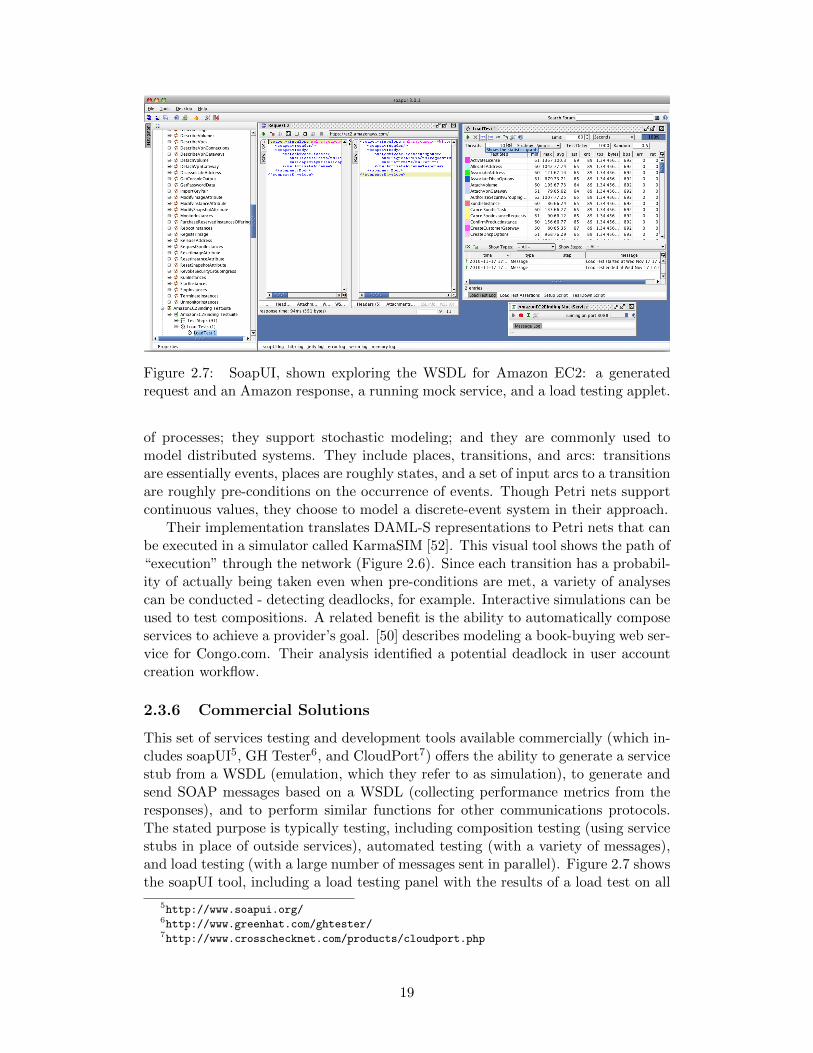
Figure 2.7: SoapUI, shown exploring the WSDL for Amazon EC2: a generatedrequest and an Amazon response, a running mock service, and a load testing applet.
of processes; they support stochastic modeling; and they are commonly used tomodel distributed systems. They include places, transitions, and arcs: transitionsare essentially events, places are roughly states, and a set of input arcs to a transitionare roughly pre-conditions on the occurrence of events. Though Petri nets supportcontinuous values, they choose to model a discrete-event system in their approach.
Their implementation translates DAML-S representations to Petri nets that canbe executed in a simulator called KarmaSIM [52]. This visual tool shows the path of“execution” through the network (Figure 2.6). Since each transition has a probabil-ity of actually being taken even when pre-conditions are met, a variety of analysescan be conducted - detecting deadlocks, for example. Interactive simulations can beused to test compositions. A related benefit is the ability to automatically composeservices to achieve a provider’s goal. [50] describes modeling a book-buying web ser-vice for Congo.com. Their analysis identified a potential deadlock in user accountcreation workflow.
2.3.6 Commercial Solutions
This set of services testing and development tools available commercially (which in-cludes soapUI5, GH Tester6, and CloudPort7) offers the ability to generate a servicestub from a WSDL (emulation, which they refer to as simulation), to generate andsend SOAP messages based on a WSDL (collecting performance metrics from theresponses), and to perform similar functions for other communications protocols.The stated purpose is typically testing, including composition testing (using servicestubs in place of outside services), automated testing (with a variety of messages),and load testing (with a large number of messages sent in parallel). Figure 2.7 showsthe soapUI tool, including a load testing panel with the results of a load test on all
5http://www.soapui.org/6http://www.greenhat.com/ghtester/7http://www.crosschecknet.com/products/cloudport.php
19
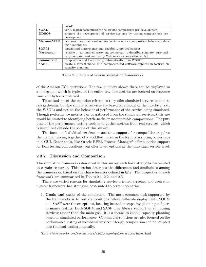
Goals
SOAD verify logical correctness of the service composition pre-development
DDSOS support the development of service systems by testing compositions pre-development
MaramaMTE help meet non-functional requirements in service composition before and dur-ing development
SOPM understand performance and scalability pre-deployment
Narayanan “enable ... automated reasoning technology to describe, simulate, automati-cally compose, test and verify Web service compositions” [50]
Commercial composition and load testing automatically from WSDLs
SASF create a virtual model of a componentized software application focused oncapacity planning
Table 2.1: Goals of various simulation frameworks.
of the Amazon EC2 operations. The raw numbers shown there can be displayed ina line graph, which is typical of the entire set. The metrics are focused on responsetime and bytes transferred.
These tools meet the inclusion criteria as they offer simulated services and met-rics gathering, but the simulated services are based on a model of the interface (i.e.,the WSDL) and not on the behavior of performance of the service being simulated.Though performance metrics can be gathered from the simulated services, their usewould be limited to identifying bottle-necks or incompatible compositions. The pur-pose of the performance testing tools is to gather metrics from real services, whichis useful but outside the scope of this survey.
The focus on individual services means that support for composition requiresthe manual piecing together of a workflow, often in the form of scripting or perhapsin a GUI. Other tools, like Oracle BPEL Process Manager8 offer superior supportfor load testing compositions, but offer fewer options at the individual service level.
2.3.7 Discussion and Comparison
The simulation frameworks described in this survey each have strengths best-suitedto certain scenarios. This section describes the differences and similarities amongthe frameworks, based on the characteristics defined in §2.2. The properties of eachframework are summarized in Tables 2.1, 2.2, and 2.3.
There are varied reasons for simulating service-oriented systems, and each sim-ulation framework has strengths best-suited to certain scenarios.
1. Goals and tasks of the simulation. The most common task supported bythe frameworks is to test compositions before full-scale deployment. SOPMand SASF were the exceptions, focusing instead on capacity planning and per-formance testing. Both SOPM and SASF offer library support for composingservices; rather than the main goal, it is a means to enable capacity planningbased on simulated performance. Commercial solutions are also focused on theperformance testing of individual services, though composition can be scriptedinto the load testing manually.
8http://www.oracle.com/technetwork/middleware/bpel/overview/index.html
20
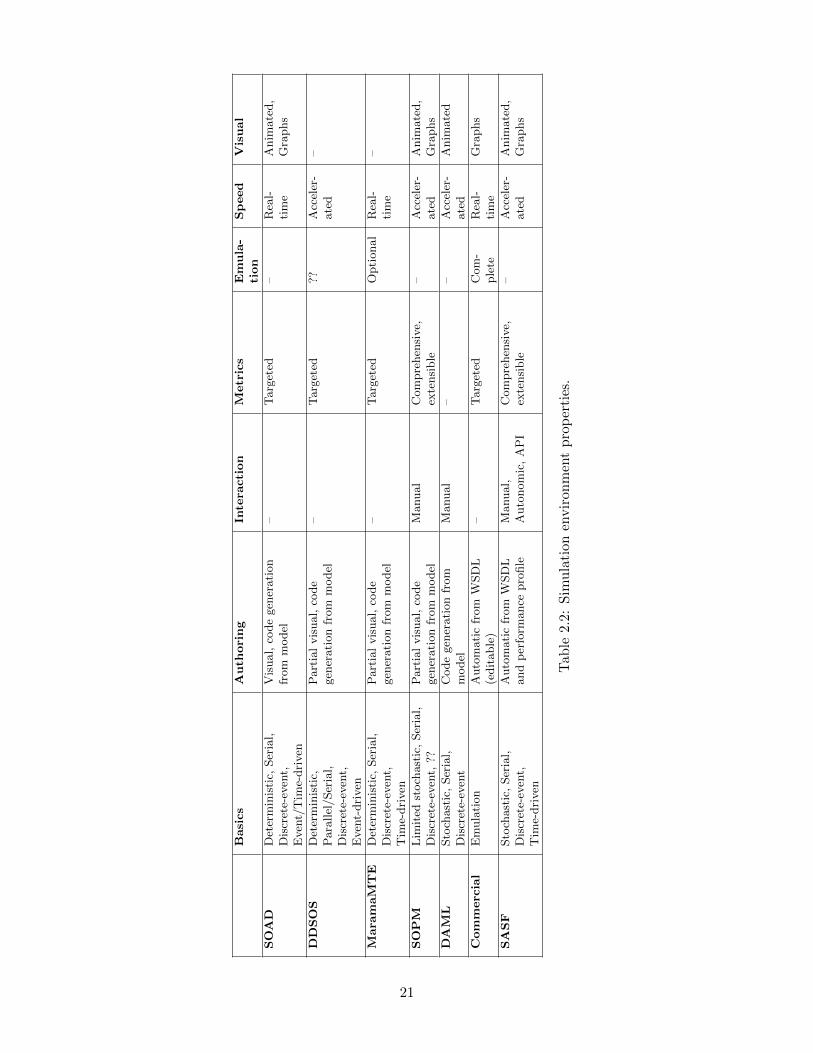
Basics
Auth
oring
Inte
raction
Metrics
Emula-
tion
Speed
Visual
SOAD
Det
erm
inis
tic,
Ser
ial,
Dis
cret
e-ev
ent,
Even
t/T
ime-
dri
ven
Vis
ual,
code
gen
erati
on
from
model
–T
arg
eted
–R
eal-
tim
eA
nim
ate
d,
Gra
phs
DDSOS
Det
erm
inis
tic,
Para
llel
/Ser
ial,
Dis
cret
e-ev
ent,
Even
t-dri
ven
Part
ial
vis
ual,
code
gen
erati
on
from
model
–T
arg
eted
??A
ccel
er-
ate
d–
Mara
maM
TE
Det
erm
inis
tic,
Ser
ial,
Dis
cret
e-ev
ent,
Tim
e-dri
ven
Part
ial
vis
ual,
code
gen
erati
on
from
model
–T
arg
eted
Opti
onal
Rea
l-ti
me
–
SOPM
Lim
ited
stoch
ast
ic,
Ser
ial,
Dis
cret
e-ev
ent,
??P
art
ial
vis
ual,
code
gen
erati
on
from
model
Manual
Com
pre
hen
sive,
exte
nsi
ble
–A
ccel
er-
ate
dA
nim
ate
d,
Gra
phs
DAM
LSto
chast
ic,
Ser
ial,
Dis
cret
e-ev
ent
Code
gen
erati
on
from
model
Manual
––
Acc
eler
-ate
dA
nim
ate
d
Commerc
ial
Em
ula
tion
Auto
mati
cfr
om
WSD
L(e
dit
able
)–
Targ
eted
Com
-ple
teR
eal-
tim
eG
raphs
SASF
Sto
chast
ic,
Ser
ial,
Dis
cret
e-ev
ent,
Tim
e-dri
ven
Auto
mati
cfr
om
WSD
Land
per
form
ance
pro
file
Manual,
Auto
nom
ic,
AP
IC
om
pre
hen
sive,
exte
nsi
ble
–A
ccel
er-
ate
dA
nim
ate
d,
Gra
phs
Tab
le2.
2:S
imu
lati
onen
vir
onm
ent
pro
per
ties
.
21
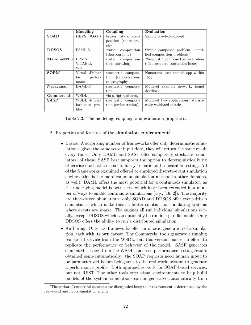
Modeling Coupling Evaluation
SOAD DEVS (SOAD) broker, static com-position (choreogra-phy)
Simple proof-of-concept
DDSOS PSML-S static composition(choreography)
Simple composed problem, identi-fied composition problems
MaramaMTE BPMN,ViTABaL-WS
static composition(orchestration)
“Simplisti” composed service, iden-tified resource contention issues
SOPM Visual, JMeterfor perfor-mance
stochastic composi-tion (orchestration,choreography
Numerous uses; sample app within15%
Narayanan DAML-S stochastic composi-tion
Modeled example network, founddeadlock
Commercial WSDL via script authoring –
SASF WSDL + per-formance pro-files
stochastic composi-tion (orchestration)
Modeled two applications; statisti-cally validated metrics
Table 2.3: The modeling, coupling, and evaluation properties.
2. Properties and features of the simulation environment9.
• Basics: A surprising number of frameworks offer only deterministic simu-lations: given the same set of input data, they will return the same resultevery time. Only DAML and SASF offer completely stochastic simu-lators; of these, SASF best supports the option to deterministically fixotherwise stochastic elements for systematic and repeatable testing. Allof the frameworks examined offered or employed discrete-event simulationengines (this is the more common simulation method in other domains,as well). DAML offers the most potential for a continuous simulator, asthe underlying model is petri nets, which have been extended in a num-ber of ways to enable continuous simulations (e.g., [16, 2]). The majorityare time-driven simulations; only SOAD and DDSOS offer event-drivensimulations, which make them a better solution for simulating systemswhere events are sparse. The engines all run individual simulations seri-ally, except DDSOS which can optionally be run in a parallel mode. OnlyDDSOS offers the ability to run a distributed simulation.
• Authoring: Only two frameworks offer automatic generation of a simula-tion, each with its own caveat. The Commercial tools generate a runningreal-world service from the WSDL, but this version makes no effort toreplicate the performance or behavior of the model. SASF generatessimulated services from the WSDL, but uses performance testing resultsobtained semi-automatically: the SOAP requests need human input tobe parameterized before being sent to the real-world system to generatea performance profile. Both approaches work for SOAP-based services,but not REST. The other tools offer visual environments to help buildmodels of the system; simulations can be generated automatically from
9The various Commercial solutions are disregarded here; their environment is determined by thereal-world and not a simulation engine.
22
these models. If a WSDL does not exist, a visual tool for modeling is abetter option. Some frameworks (like DAML) use the same approach tomodel the service at design time and guide implementation, which givesdual-purpose to the modeling stage.
• Interaction: Here SASF is quite distinct, as compared to the other ap-proaches. Only SOPM, DEVS, and DAML offer even the basic abilityto interact with a running simulation; the others are launch-and-forget.SASF goes further, offering both an API and internal functions for modi-fying the parameters of a running simulation (including properties of thesimulation environment and the simulated application).
• Metrics gathering: Again SASF is a standout; the features and APIsenabling the collection and dissemination of metrics require minimumeffort by the simulation author. Only SOPM offers such customizablemetrics gathering.
• Visual: The standard here is the generation of visual depictions of metricsor of the system architecture, often animated. Only DDSOS and Mar-maMTE fall short in this category. SASF requires less developer effortwhen introducing additional metrics to the visualizations.
• Emulation: Commercial solutions offer total integration with real-worldservices, where simulated services can even participate in compositionswith already implemented services (with syntactically correct but seman-tically meaningless data). Only SASF and MarmaMTE offer any abilityto integrate real-world services with simulated services that accuratelyreflect the behavior of the service.
• Speed: As a consequence of their emulation abilities, the Commercialand MarmaMTE frameworks cannot run faster than a real-world service.SOAD also has this constraint. SASF runs at an accelerated pace, exceptwhen in optional emulation mode.
3. Modeling language and methods, abstract representations, or formalisms.SASF and commercial solutions rely on the existing model of a service asexpressed in WSDL. This is advantageous if the service already exists and isdescribed using a WSDL; if not, the increases expressiveness of other modelsmay be superior. The others use typically more rigorous formalisms that allowthe use of formal methods and proofs. SOPM offers a purely visual model.
4. Support for service coupling. All of the frameworks support compositionto some extent. MarmaMTE is notable for its use of BPMN as a modellinglanguage.
5. Evaluation method. SASF is noteworthy, as it has been used to model full-size real-world componentized software systems and statistically validated toaccurately predict service performance, then used to reason about the system.SOPM has also been used to address research problems.
23

2.4 Value, Quality, and Cost
To make configuration decisions by reasoning with simulation-generated data, atarget must be defined. This target is often defined using technical metrics suchas response time or throughput. Though these metrics are easily definable andmeasurable, they are not sufficient when asking non-technical users to understandor compare configurations. As discussed in Section 2.1.1, SLAs are often describedin technical terms not accessible to business users. This section turns to marketingand business literature to understand higher-order attributes like value, quality,satisfaction, and cost. In particular, how perceived value, quality, and cost informthe decision-making process is described.
Value is not a constant definition with all consumers, and it varies from personto person and from product to product. Zeithaml [82] offers an overall definition:“perceived value is the consumer’s overall assessment of the utility of a product basedon perceptions of what is received and what is given.” To us, that means “they do acost-benefit analysis”. There is a trade-off inherent to value: customers are willingto sacrifice some attributes in exchange for gains in other attributes. For example,they may give up convenient twist-top lids in exchange for 100% pure juice, or theymay pay more for a product they consider environmentally friendly. Decisions canbe guided by single attributes (e.g., monetary cost) or some combination. In simpleterms, one can think of perceived value as “what I get for what I give”, where eachindividual may consider various attributes to ‘give’ in exchange for various attributesthey ‘get’. The total of what is given up (or sacrificed) is the perceived cost.
Researchers agree that value is a conclusion reached based on a variety of factorsand attributes. Essentially, low level attributes imply quality, quality and cost implyvalue, value affects value to me personally. Sawyer and Dickson [68] defined valueas “a ratio of attributes weighted by their evaluations divided by price weighted byits evaluation”. They separate price from the other attributes. Though this is aformula that implies numeric analysis, it can be difficult to quantify the variables.
Quality is, at an abstract level, a measure of excellence or superiority [82]. It isnot an attribute; rather, it is a high-level construct formed in the minds of individualsbased on their assessment of a product or service. Research distinguishes betweenactual quality and perceived quality. Actual quality is some quantifiable and verifiablemeasure of excellence, compared to some norm or ideal. We measure water quality inparts-per-million of substances that should not be in pure (ideal) water. We measuremanufacturing quality in terms of the number of defects per item produced, with anideal of “0”. Perceived quality is a more complex measure that factors in customerexpectations, customer experience, comparator sets, and other factors to form aglobal assessment of quality. It is a customer’s judgment about the superiority orexcellence of a product. It is this definition that most influences perceived value.
Perceived quality, in its reliance on experience and knowledge, is assessed basedon what the consumer knows about the product and all competing products. Whichproducts are ‘competing’ is up to the consumer (Ford might think their competitionis Toyota, but to some consumers it may be Vespa).
There are varying schools of thought on how to assess quality. Perhaps thebest known is SERVQUAL [59], which assesses quality based on the gap betweenwhat the consumer expects and what they actually experience. Over the 25 yearssince was proposed, it has been refined several times (e.g., [57, 83]). It measures
24
the gap between expectation and perception in five primary categories: Reliability,Assurance, Tangibles, Empathy, and Responsiveness (RATER). It is driven funda-mentally by satisfaction, where the smaller the gaps, the greater the satisfaction.Over the same time period, it has also attracted criticisms and alternatives. Oneof the best known contenders is SERVPERF [13], which is performance-based orattitude-based: Cronin and Taylor assert that perceived service quality can be bestmeasured by a customer’s “perceived” attitude about the service. The debate (e.g.,[14, 60]) has continued since and will not be re-produced here10. This backgroundsection is influenced by the gap/satisfaction model.
Lutz [43] proposes that we consider two other forms of quality: “affective quality”and “cognitive quality”. A cognitive judgment is one based primarily on attributesthat can be determined without actually consuming a product (brand, reputation,packaging), while affective quality is determined by actual experience. He suggeststhat service quality is an affective judgment: that is, global assessment of servicequality is based on personal experience.§2.4.2 presents a set of propositions that help understand perceived value, per-
ceived quality, and perceived cost. These propositions motivate an SLA negotiationapproach described in Chapter 5. The propositions relate to products; to assesstheir applicability, we must first establish that a web service shares properties withtraditional definitions of products (§2.4.1).
2.4.1 Web Services as Products
In business and marketing literature, organizations can traditionally market prod-ucts and/or services. The intuition of these concepts is easily determined; however,the distinction between them is more subtle. The academic community does notentirely agree on the distinction. The idea of a service offered online without evertalking to a person was still a foreign idea when much of the foundational literaturein service quality was written. The expectation given the name “web service” isthat it would align with the notion of a service in marketing literature. In fact, aweb service has qualities in common with both.
Zeithaml, Parasuraman, & Berry [58] conducted a review of services literatureand concluded that the prevailing characterizations of services were “intangibility,inseparability of production and consumption, heterogeneity, and perishability”.That is, services are difficult to measure, they are consumed at the moment they areproduced, they are not always consistent, and they cannot be stored. The difficultyin measuring the outcome of a service led to the consideration of the process of aservice rather than the outcome (e.g. [47, 53]). Table 2.4 lists how electronic webservices compare with this traditional definition.
Nilsson explored intangibility in more depth and concluded that there are fewobjective reference points for consumers to use in perceiving value in services. Anycues are ambiguous at best; therefore, the personnel offering the services can in-fluence how the consumer perceives quality. The literature in marketing frequentlyrefers to “service encounters”: quality assessment, decision-making, and so forth are
10The notion that a one paragraph summary can adequately represent almost 3 decades of ongoingdebate, refinement, and extension is, of course, ridiculous. Google Scholar reports 6776 citations forthe original SERVQUAL paper and 3557 for SERVPERF, and in the thousands for the key debatepapers.
25
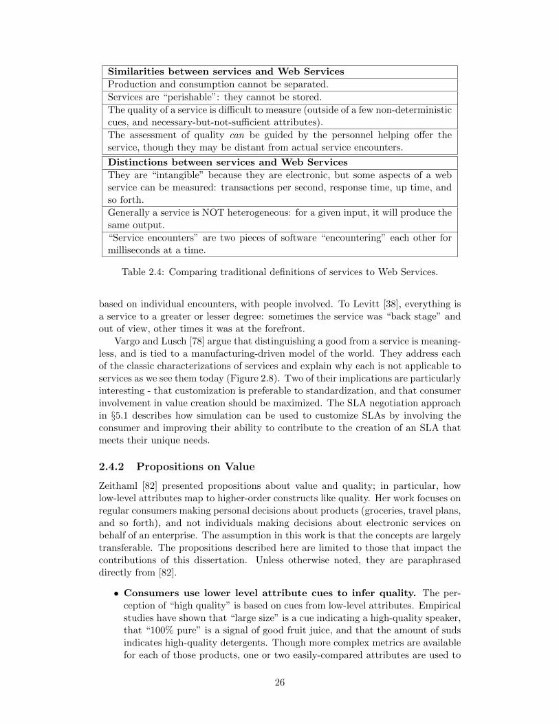
Similarities between services and Web Services
Production and consumption cannot be separated.
Services are “perishable”: they cannot be stored.
The quality of a service is difficult to measure (outside of a few non-deterministiccues, and necessary-but-not-sufficient attributes).
The assessment of quality can be guided by the personnel helping offer theservice, though they may be distant from actual service encounters.
Distinctions between services and Web Services
They are “intangible” because they are electronic, but some aspects of a webservice can be measured: transactions per second, response time, up time, andso forth.
Generally a service is NOT heterogeneous: for a given input, it will produce thesame output.
“Service encounters” are two pieces of software “encountering” each other formilliseconds at a time.
Table 2.4: Comparing traditional definitions of services to Web Services.
based on individual encounters, with people involved. To Levitt [38], everything isa service to a greater or lesser degree: sometimes the service was “back stage” andout of view, other times it was at the forefront.
Vargo and Lusch [78] argue that distinguishing a good from a service is meaning-less, and is tied to a manufacturing-driven model of the world. They address eachof the classic characterizations of services and explain why each is not applicable toservices as we see them today (Figure 2.8). Two of their implications are particularlyinteresting - that customization is preferable to standardization, and that consumerinvolvement in value creation should be maximized. The SLA negotiation approachin §5.1 describes how simulation can be used to customize SLAs by involving theconsumer and improving their ability to contribute to the creation of an SLA thatmeets their unique needs.
2.4.2 Propositions on Value
Zeithaml [82] presented propositions about value and quality; in particular, howlow-level attributes map to higher-order constructs like quality. Her work focuses onregular consumers making personal decisions about products (groceries, travel plans,and so forth), and not individuals making decisions about electronic services onbehalf of an enterprise. The assumption in this work is that the concepts are largelytransferable. The propositions described here are limited to those that impact thecontributions of this dissertation. Unless otherwise noted, they are paraphraseddirectly from [82].
• Consumers use lower level attribute cues to infer quality. The per-ception of “high quality” is based on cues from low-level attributes. Empiricalstudies have shown that “large size” is a cue indicating a high-quality speaker,that “100% pure” is a signal of good fruit juice, and that the amount of sudsindicates high-quality detergents. Though more complex metrics are availablefor each of those products, one or two easily-compared attributes are used to
26

Bitner 2000). We argue that the intangibility, heterogene-ity, inseparability, and perishability characterizations failto delineate services from goods adequately. We also arguethat (a) these characteristics are inaccurate and misleadingabout the nature of market offerings, (b) their implicationsfor marketing strategy are contradictory to a market andconsumer orientation, and (c) their implications should beinverted (see Table 1). In short, what we have learned bystudying service can and should be applied to all of ex-change. Although this argument is consistent with our pro-posed, revised positive definition of service, it is notcontingent on the definition.
Intangibility
The myth. The primary distinguishing characteristic ofservices in relation to goods is normally considered to beintangibility. Despite the appealing nature of such a clear-cut line of demarcation, at worst it does not hold up, and atbest it has little or no relevance. Several service scholars(e.g., Shostack 1977; Swartz, Bowen, and Brown 1992)have noted that by the intangibility criteria there are nopure services or goods. Their argument is based on the ob-servation that essentially all goods have a service compo-
nent, whereas essentially all services have some form oftangible representation.
Partially because the most that can be done with thischaracteristic is to attempt to array goods and services on acontinuum according to the relative degree of tangibility, anumber of scholars (e.g., Gummesson 1995, 2000; Rust1998) have questioned what its delineation really pro-vides. Iacobucci (1992) investigated the perceived ser-vices versus goods nature and the perceived tangibility of awide array of offerings and found that “while goods are in-deed perceived to be relatively more tangible than ser-vices, all these stimuli are perceived to be rather tangible inan absolute sense” and concluded that “the tangibility rat-ings are an example of where the data were not closelyaligned with theoretical expectations” (pp. 33, 49).Beaven and Scotti (1990) maintained that “service pro-cesses and their outcomes result in specific sensory impres-sions that are stored in the mind as concrete, tangiblefacts,” and thus the distinction is “illusionary” (p. 8). Con-versely, Gummesson (2000) argued, “If I am operated onin the hospital I am myself the ‘machine,’ the ‘object of re-pair and maintenance.’ It is unpleasant; it may hurt. I canget better, worse, or die. Can it get much more tangible?”(p. 123)
Vargo, Lusch / SERVICE MARKETING MYTHS 327
TABLE 1Limitations and Implications of
Distinguishing Characteristics of Services
Dimension Dispelling the Myth Perspective Inverted Implication
IntangibilityServices lack the tactile quality
of goodsServices often have tangible resultsTangible goods are often purchased
for intangible benefitsTangibility can be a limiting factor
in distribution
The focus on manufactured outputis myopic and goods oriented
Consumers buy service even whena tangible product is involved
Intangibles such as brand image aremore important
Unless tangibility has a marketingadvantage, it should be reducedor eliminated if possible
HeterogeneityUnlike goods, services cannot
be standardizedTangible goods are often heteroge-
neousMany services are relatively stan-
dardized
Homogeneity in production isviewed heterogeneously in con-sumption
The normative marketing goalshould be customization, ratherthan standardization
InseparabilityUnlike goods, services are
simultaneously produced andconsumed
The consumer is always involvedin the “production” of the value
Only manufacturing benefits fromefficiency of separability
Separability limits marketability
The normative marketing goalshould be to maximize consumerinvolvement in value creation
PerishabilityServices cannot be produced
ahead of time and inventoriedTangible goods are perishableMany services result in long-
lasting benefits
Value is created at the point of con-sumption, not in the factory
The normative goal of the enter-prise should be to reduce inven-tory and maximize service flows
Both tangible and intangible capa-bilities can be inventoried
Inventory represents an additionalmarketing cost
Figure 2.8: Limitations of the distinguishing characteristics of services, from [78].
serve as reliable signals of quality. Consumers instinctively look for low-levelattributes that consistently signal high-quality services.
For complex decisions, relying on one or several low-level attributes can bemisleading. To avoid this, a high-level or aggregate attribute should be usedto help decision-makers determine quality more explicitly, rather than relyingon each individual to choose their own set of low-level attributes.
• The intrinsic product attributes that signal quality are product-specific, but dimensions of quality can be generalized to productclasses or categories. Researchers divide attributes into intrinsic (physicalcomposition of the product: color, shape, size, taste) and extrinsic (product-related but not part of the product: brand, price, level of advertising). Intrinsicproperties are consumed as the product is consumed. Of course, there isambiguity here.
The few intrinsic attributes a consumer considers when determining qualityvary by product. The cues that signal quality for juice differ from the cuesfor lamps. Even similar products show variation: thick tomato juice is good,thick grape juice is bad. However, some aspects of quality apply generally towhole classes of products. The more abstract an attribute, the more likely itis to apply to a large set of products. Comparing two different things, likestereos and vacations, requires consumers to use very abstract concepts like“entertainment value”.
When asked to consider service industries, Parasuraman [58] found that con-sumers consistently judged quality based on reliability, empathy, assurance,responsiveness, and tangibles.
• Extrinsic cues serve as generalized quality indicators across brands,products, and categories. Unlike intrinsic cues, most extrinsic cues are
27
already abstract and generalizable across product classes. Brand, price, war-ranty, seals of approval, and endorsements are all extrinsic cues. Research inthis area has shown that in the absence of all other information, high pricemeans high quality. Brand name offers a bundle of information that can in-tellectually be the same as experiencing the product: if you’ve used a serviceprovider to book a flight and preferred it, you may be more likely to rent acar from the same provider.
• When customer’s rely on intrinsic or extrinsic attributes. Consumersdepend on intrinsic attributes more than extrinsic attributes:
1. at the point of consumption,
2. in pre-purchase situations when intrinsic attributes are search attributes(rather than experience attributes), and
3. when the intrinsic attributes have high predictive value.
Consumers depend on extrinsic attributes more than intrinsic attributes:
1. in initial purchase situations when intrinsic cues are not available (e.g.,for services),
2. when evaluation of intrinsic cues requires more effort and time than theconsumer perceives is worthwhile, and
3. when quality is difficult to evaluate (experience and credence goods).
Intrinsic attributes are more useful while consuming a product: when drinkinga beverage, you measure your satisfaction by the taste, not by the brand name.Search attributes are those that can be assessed prior to purchase (e.g. “100%pure” for juice, “no blemishes” for fruit), whereas experience attributes areassessed only during consumption (e.g., “smooth” for juice, “not under- orover-ripe” for fruit). In pre-purchase situations, intrinsic cues are used whenthey can be assessed prior to purchase. When they cannot be, extrinsic cuesare used. Services have few intrinsic cues, and those available can typicallynot be assessed until the service encounter has begun. Thus, services arefrequently initially judged using only extrinsic cues.
Intrinsic attributes are used when they can be readily assessed and are knownto have high predictive value. If there are barriers to evaluating intrinsicattributes, extrinsic ones will be used instead. Similarly, if easily evaluatedintrinsic cues are not sufficient to differentiate between two products (e.g.,identical memory and processor configurations), the consumer will resort toextrinsic cues.
Intrinsic attributes are useful and generally preferred, but are limited by beingrequiring experience to assess them. This is a strong motivator for the use ofsimulation: experience can be simulated, allowing the use of intrinsic attributesin situations where it would otherwise be impossible or cost-prohibitive.
• Monetary price is not the only sacrifice perceived by consumers.This point is perhaps obvious; when you make a decision, you weigh manytrade-offs, only one is price. The literature divides the elements of a purchase
28
decision into two sides: what you give versus what you get. Those things you“give” are considered sacrifices, and this includes price. However, consumersare also aware that there are other sacrifices. If you pay a lower price but haveto assemble your own furniture, the additional work required is part of thesacrifice. Travel time, search time, evaluation time, maintenance time, andmore may all be factored in to the total “sacrifice”. The result is a distinctionbetween the actual price and the perceived price. People have different ways ofencoding the price or sacrifice, for example: “expensive”, “a bargain”, “you getwhat you pay for”. The overall sacrifice is part of the equation for determiningperceived value.
• Extrinsic attributes serve as “value signals” and can substitute foractive weighing of benefits and costs. Consumers are generally “mind-less” [36]; there is not careful consideration so much as there is overall im-pression. “Trusted brand”, “it’s cheaper than it was last week”, and similarcues are used in place of hard facts. There are some consumers who spendtime and effort to give purchases careful consideration; Zeithaml theorizes thatmore rational evaluation is used when there is lots of information available, lotsof time, lots of processing ability, and high involvement in the purchase. Onetheory is that as the cost of the product goes up (or, as the cost of choosingthe wrong product goes up), more careful consideration is more common.
Ongoing service delivery requires more than an initial purchase decision; adecision based on facts is likely to prove more satisfying than one based oninstinct. Thus, when establishing an SLA steps should be taken to encouragerational evaluation: high involvement with the customer in establishing theSLA and furnishing the customer with as much information as they need aretwo key ways to do this.
• The perception of value depends on the frame of reference in whichthe consumer is making an evaluation. Value determination is situa-tional and depends on context. Zeithaml reports that value changes betweenpurchase time, preparation time, and consumption. The use of simulation al-lows consumers to incorporate their (predicted) value at consumption time atpurchase time, limiting “buyer remorse”.
• Perceived value affects the relationship between quality and pur-chase. Customers do not always purchase the highest quality option; theymake a decision that balances their perceived quality and perceived sacrifice:their perceived value. The trade-off is the key factor and should be incorpo-rated into decision support tools.
2.5 Capacity Planning and Configuration Management
The problem of capacity planning is very general and highly relevant to manufac-turing and service-delivery business strategy. According to Balachandran et al. [5],the cost of capacity resources typically account for 30% to 60% of the total costsin manufacturing and 70% to 80% of the total costs in service organizations. This
29
high cost percentage gives rise to the need for capacity planning, so that organi-zations can obtain all necessary resources at once, ahead of time, as opposed onas-needed basis, which would potentially further increase the cost ratio. In their1997 work, they considered the general problem where product production requiresresource consumption (under some stochastic model) and product price is a functionof product cost (as implied by the cost of the consumed resources) and a randomprofit. They distinguished between ‘soft’ and ‘hard’ constraints on resources that can(and cannot) be acquired on an as-needed basis in case of shortfall. Note that thisformulation clearly relates the problems of capacity planning at deployment config-uration time and autonomic capacity adjustment at run time. Through simulationexperiments they found that simplifying capacity planning to focus on an expectedbottleneck resource dominates product- or resource-level capacity planning, whenall resources impose hard constraints and the firm’s product mix is significant.
More specifically, in the context of computer-based service delivery systems, re-search has been conducted on capacity planning for different types of architectures.Kant et al. [30] examined, both with analytical and simulation models, the perfor-mance behavior of a traditional symmetric multiprocessor web server, under differenttypes of benchmark loads. They found that using the virtual interface architectureimproves performance, especially in the case of workloads with increased memorybandwidth. Furthermore, they predicted that more I/O capacity is required whenthe network processing is offloaded.
Almeida and Menasce [46] developed a general method for capacity planningin client-server systems, making explicit the need for models of workloads that thearchitecture is expected to support and the way its performance may change whenaspects of the workload change. This approach is not service-focused and does notuse simulation to produce data.
Zhang et al. created R-Capriccio, a capacity-planning tool that uses availableperformance information to make predictions and decisions about future capacityrequirements [84]. The tool identifies the most popular client transactions, estimatesthe CPU requirements, and uses queueing networks to project capacity requirementsfor changing workloads. The tool is limited to CPU-bound services, and requireslogs of both server access and CPU utilization under existing load.
Finally, Rossi and Tari developed a method for web-service self-adaptation tomitigate the impact of changes in the environment on performance and resourceutilization [64]. They use middleware to move services among nodes in a clusterto balance load, based on real-time performance metrics. Services are distributedamong nodes in order to optimize an “efficiency value” derived from various perfor-mance metrics.
2.6 Autonomic Computing: Self Management
The demand for dynamic, distributed, component-driven software has led to in-creased adoption of service-oriented software systems. The nature of these systemslimits the effectiveness of design-time configuration decisions; additional copies ofservice instances may be deployed at run time; new services may be removed andnew services may be introduced in an existing composition; the provisioned networkbandwidth can be changed. This is why deploy-time and even run-time configu-
30
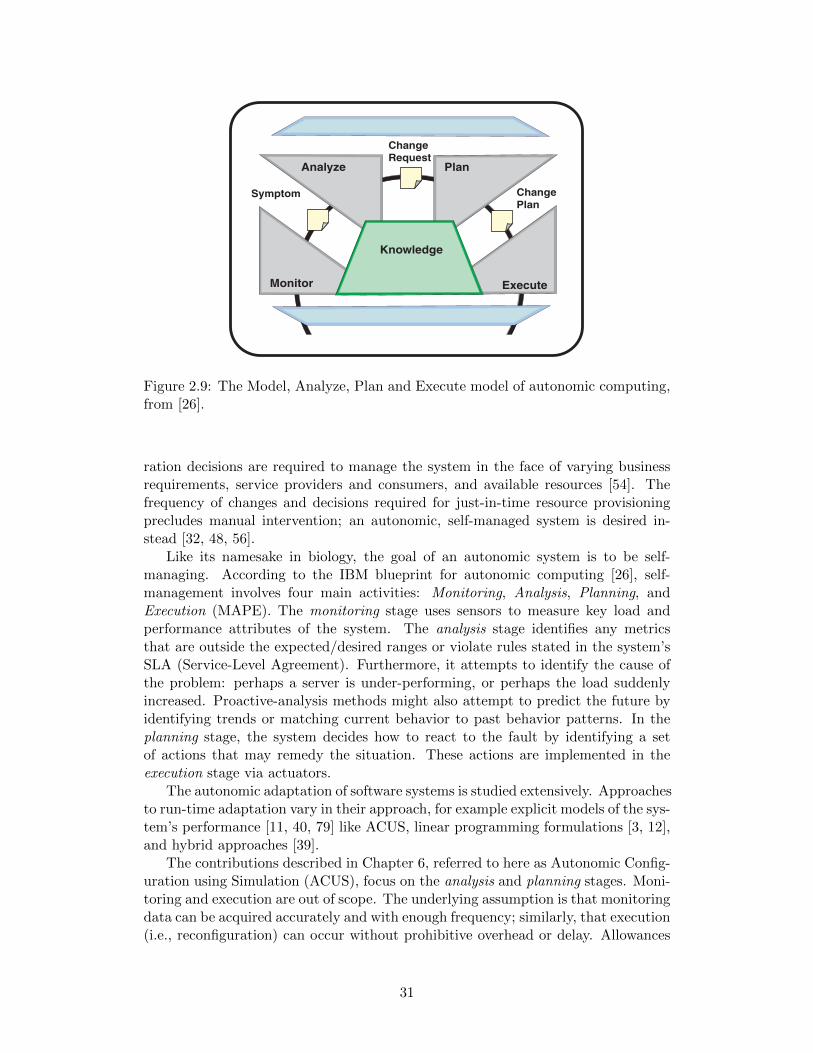
An architectural blueprint for autonomic computingPage 13
An architectural blueprint for autonomic computingPage 14
• A homogeneous group scope aggregates resources of the same type. An
example of a homogeneous group is a pool of servers that an autonomic
manager can dynamically optimize to meet certain performance and
availability thresholds.
• A heterogeneous group scope organizes resources of different types. An
example of a heterogeneous group is a combination of heterogeneous
devices and servers, such as databases, Web servers and storage
subsystems that work together to achieve common performance and
availability targets.
• A business system scope organizes a collection of heterogeneous
resources so an autonomic manager can apply its intelligent control
loop to the service that is delivered to the business. Some examples are
a customer care system or an electronic auction system. The business
system scope requires autonomic managers that can comprehend the
optimal state of business processes—based on policies, schedules and
service levels—and drive the consequences of process optimization back
down to the resource groups (both homogeneous and heterogeneous)
and even to individual resources.
These resource scopes define a set of decision-making contexts that are
used to classify the purpose and role of a control loop within the autonomic
computing architecture.
The touchpoint autonomic managers shown previously in Figure 2 are each
dedicated to a particular resource or a particular collection of resources.
Touchpoint autonomic managers also expose a sensor and an effector,
Symptom
ChangeRequest
ChangePlan
Analyze Plan
Monitor
Knowledge
Execute
Single Resource Homogeneous Group Business SystemHeterogeneous Group
Figure 3. Four common managed resource arrangements
Figure 2.9: The Model, Analyze, Plan and Execute model of autonomic computing,from [26].
ration decisions are required to manage the system in the face of varying businessrequirements, service providers and consumers, and available resources [54]. Thefrequency of changes and decisions required for just-in-time resource provisioningprecludes manual intervention; an autonomic, self-managed system is desired in-stead [32, 48, 56].
Like its namesake in biology, the goal of an autonomic system is to be self-managing. According to the IBM blueprint for autonomic computing [26], self-management involves four main activities: Monitoring, Analysis, Planning, andExecution (MAPE). The monitoring stage uses sensors to measure key load andperformance attributes of the system. The analysis stage identifies any metricsthat are outside the expected/desired ranges or violate rules stated in the system’sSLA (Service-Level Agreement). Furthermore, it attempts to identify the cause ofthe problem: perhaps a server is under-performing, or perhaps the load suddenlyincreased. Proactive-analysis methods might also attempt to predict the future byidentifying trends or matching current behavior to past behavior patterns. In theplanning stage, the system decides how to react to the fault by identifying a setof actions that may remedy the situation. These actions are implemented in theexecution stage via actuators.
The autonomic adaptation of software systems is studied extensively. Approachesto run-time adaptation vary in their approach, for example explicit models of the sys-tem’s performance [11, 40, 79] like ACUS, linear programming formulations [3, 12],and hybrid approaches [39].
The contributions described in Chapter 6, referred to here as Autonomic Config-uration using Simulation (ACUS), focus on the analysis and planning stages. Moni-toring and execution are out of scope. The underlying assumption is that monitoringdata can be acquired accurately and with enough frequency; similarly, that execution(i.e., reconfiguration) can occur without prohibitive overhead or delay. Allowances
31
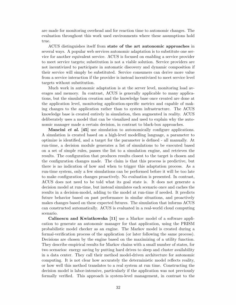
are made for monitoring overhead and for reaction time to autonomic changes. Theevaluation throughout this work used environments where these assumptions holdtrue.
ACUS distinguishes itself from state of the art autonomic approaches inseveral ways. A popular web services autonomic adaptation is to substitute one ser-vice for another equivalent service. ACUS is focused on enabling a service providerto meet service targets; substitution is not a viable solution. Service providers arenot incentivized to participate in automatic discovery and dynamic composition iftheir service will simply be substituted. Service consumers can derive more valuefrom a service interaction if the provider is instead incentivized to meet service leveltargets without substitution.
Much work in autonomic adaptation is at the server level, monitoring load av-erages and memory. In contrast, ACUS is generally applicable to many applica-tions, but the simulation creation and the knowledge base once created are done atthe application level, monitoring application-specific metrics and capable of mak-ing changes to the application rather than to system infrastructure. The ACUSknowledge base is created entirely in simulation, then augmented in reality. ACUSdeliberately uses a model that can be visualized and used to explain why the auto-nomic manager made a certain decision, in contrast to black-box approaches.
Mancini et al. [45] use simulation to autonomically configure applications.A simulation is created based on a high-level modelling language, a parameter tooptimize is identified, and a target for the parameter is defined - all manually. Atrun-time, a decision module generates a list of simulations to be executed basedon a set of simple rules, passes the list to a simulation engine, and retrieves theresults. The configuration that produces results closest to the target is chosen andthe configuration changes made. The claim is that this process is predictive, butthere is no indication of how and when to trigger this adaptation process. As arun-time system, only a few simulations can be performed before it will be too lateto make configuration changes proactively. No evaluation is presented. In contrast,ACUS does not need to be told what its goal state is. It does not generate adecision model at run-time, but instead simulates each scenario once and caches theresults in a decision-model, adding to the model at run-time if needed. It predictsfuture behavior based on past performance in similar situations, and proactivelymakes changes based on these expected futures. The simulation that informs ACUScan constructed automatically. ACUS is evaluated in a real-world cloud computingscenario.
Calinescu and Kwiatkowska [11] use a Markov model of a software appli-cation to generate an autonomic manager for that application, using the PRISMprobabilistic model checker as an engine. The Markov model is created during aformal-verification process of the application (or later following the same process).Decisions are chosen by the engine based on the maximizing of a utility function.They describe empirical results for Markov chains with a small number of states, fortwo scenarios: energy saving by putting hard drives to sleep and cluster availabilityin a data center. They call their method model-driven architecture for autonomiccomputing. It is not clear how accurately the deterministic model reflects reality,or how well this method translates to a real system at run time. Constructing thedecision model is labor-intensive, particularly if the application was not previouslyformally verified. This approach is system-level management, in contrast to the
32
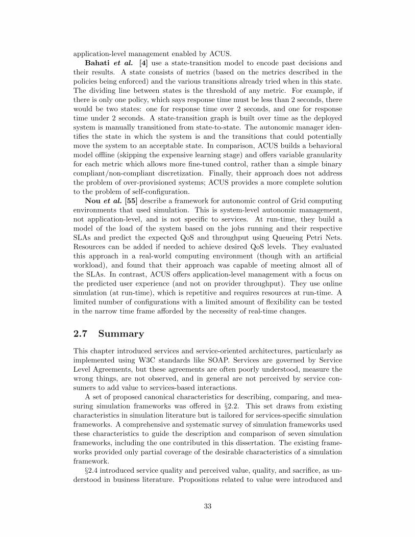
application-level management enabled by ACUS.Bahati et al. [4] use a state-transition model to encode past decisions and
their results. A state consists of metrics (based on the metrics described in thepolicies being enforced) and the various transitions already tried when in this state.The dividing line between states is the threshold of any metric. For example, ifthere is only one policy, which says response time must be less than 2 seconds, therewould be two states: one for response time over 2 seconds, and one for responsetime under 2 seconds. A state-transition graph is built over time as the deployedsystem is manually transitioned from state-to-state. The autonomic manager iden-tifies the state in which the system is and the transitions that could potentiallymove the system to an acceptable state. In comparison, ACUS builds a behavioralmodel offline (skipping the expensive learning stage) and offers variable granularityfor each metric which allows more fine-tuned control, rather than a simple binarycompliant/non-compliant discretization. Finally, their approach does not addressthe problem of over-provisioned systems; ACUS provides a more complete solutionto the problem of self-configuration.
Nou et al. [55] describe a framework for autonomic control of Grid computingenvironments that used simulation. This is system-level autonomic management,not application-level, and is not specific to services. At run-time, they build amodel of the load of the system based on the jobs running and their respectiveSLAs and predict the expected QoS and throughput using Queueing Petri Nets.Resources can be added if needed to achieve desired QoS levels. They evaluatedthis approach in a real-world computing environment (though with an artificialworkload), and found that their approach was capable of meeting almost all ofthe SLAs. In contrast, ACUS offers application-level management with a focus onthe predicted user experience (and not on provider throughput). They use onlinesimulation (at run-time), which is repetitive and requires resources at run-time. Alimited number of configurations with a limited amount of flexibility can be testedin the narrow time frame afforded by the necessity of real-time changes.
2.7 Summary
This chapter introduced services and service-oriented architectures, particularly asimplemented using W3C standards like SOAP. Services are governed by ServiceLevel Agreements, but these agreements are often poorly understood, measure thewrong things, are not observed, and in general are not perceived by service con-sumers to add value to services-based interactions.
A set of proposed canonical characteristics for describing, comparing, and mea-suring simulation frameworks was offered in §2.2. This set draws from existingcharacteristics in simulation literature but is tailored for services-specific simulationframeworks. A comprehensive and systematic survey of simulation frameworks usedthese characteristics to guide the description and comparison of seven simulationframeworks, including the one contributed in this dissertation. The existing frame-works provided only partial coverage of the desirable characteristics of a simulationframework.§2.4 introduced service quality and perceived value, quality, and sacrifice, as un-
derstood in business literature. Propositions related to value were introduced and
33
how they should influence the formation of service level agreements was described.Customization is preferable to standardization, consumer involvement in value cre-ation should be maximized, the best way to measure and predict value and qualityis based on experience with the product, that monetary sacrifice is not the onlyrelevant trade-off when calculating value, and that the highest quality option isn’talways the right choice (the trade-off is more important).
Existing approaches to configuration management (§2.5) do not make use ofsimulation to predict performance; instead, data from real-world deployed systemsis used directly. This data is more expensive to produce, though is by definitionaccurate. When simulation is used, it is used to predict bottlenecks and resourcecontention issues; the work described in this dissertation takes a different approach,focusing on maximizing user-centric value and explicitly guiding users through man-aging trade-offs.
Related work in the area of autonomic computing was reviewed in §2.6; thoughstate-transition models have been used before to construct an abstract representa-tion of the behavior, their construction based on simulation-generated data is novel.There is little real-world validation of autonomic self-configuration approaches. Au-tonomic work in services focuses on substituting services with other services thatperform the same function; the approach taken in this dissertation is to insteadre-configure the original service to make its continued use possible. The approachdescribed in this dissertation is at the application-level, instead of the more commonapproach of hardware-level or infrastructure-level management. Finally, a short-coming of autonomic approaches is they are difficult to understand or explain; thesimulation-generated narrative of predicted performance and the visualizable state-transition model presented here allow re-configuration decisions to be explained.
34
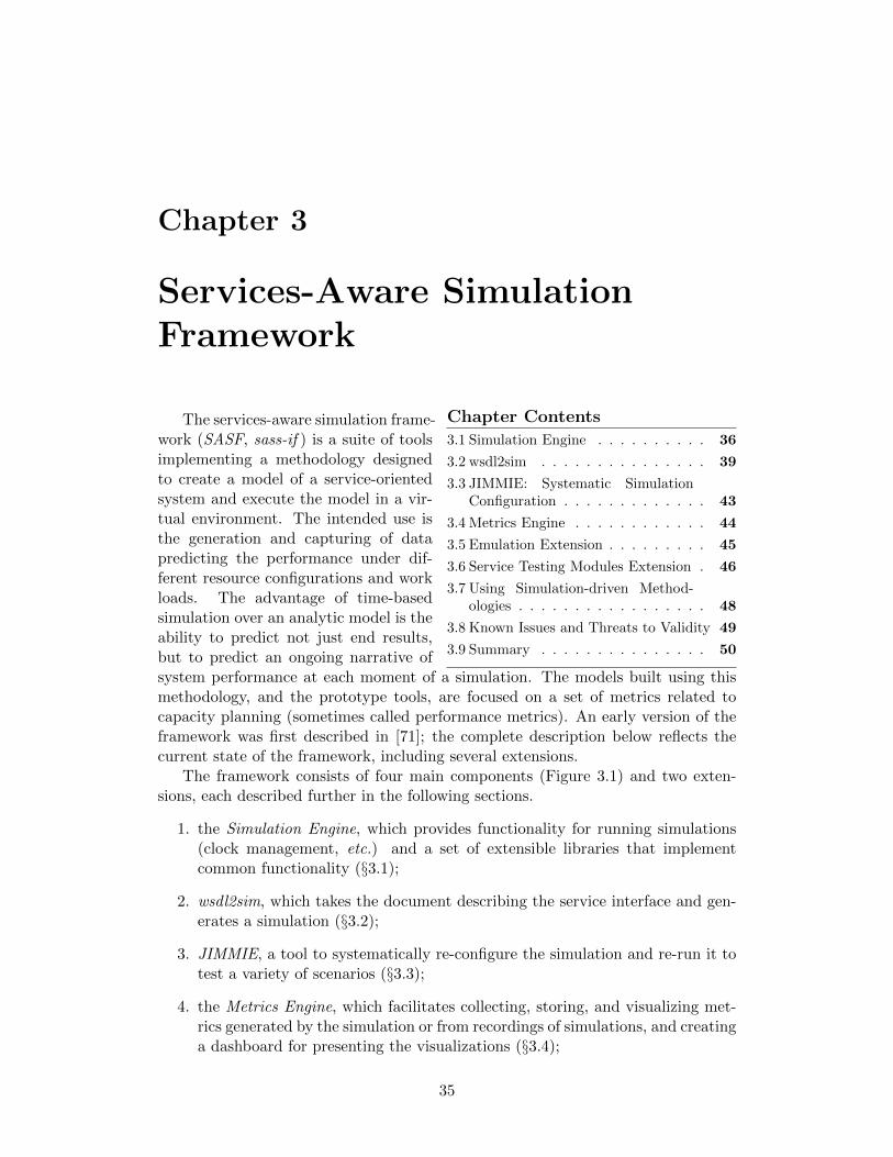
Chapter 3
Services-Aware SimulationFramework
Chapter Contents
3.1 Simulation Engine . . . . . . . . . . 36
3.2 wsdl2sim . . . . . . . . . . . . . . . 39
3.3 JIMMIE: Systematic SimulationConfiguration . . . . . . . . . . . . . 43
3.4 Metrics Engine . . . . . . . . . . . . 44
3.5 Emulation Extension . . . . . . . . . 45
3.6 Service Testing Modules Extension . 46
3.7 Using Simulation-driven Method-ologies . . . . . . . . . . . . . . . . . 48
3.8 Known Issues and Threats to Validity 49
3.9 Summary . . . . . . . . . . . . . . . 50
The services-aware simulation frame-work (SASF, sass-if ) is a suite of toolsimplementing a methodology designedto create a model of a service-orientedsystem and execute the model in a vir-tual environment. The intended use isthe generation and capturing of datapredicting the performance under dif-ferent resource configurations and workloads. The advantage of time-basedsimulation over an analytic model is theability to predict not just end results,but to predict an ongoing narrative ofsystem performance at each moment of a simulation. The models built using thismethodology, and the prototype tools, are focused on a set of metrics related tocapacity planning (sometimes called performance metrics). An early version of theframework was first described in [71]; the complete description below reflects thecurrent state of the framework, including several extensions.
The framework consists of four main components (Figure 3.1) and two exten-sions, each described further in the following sections.
1. the Simulation Engine, which provides functionality for running simulations(clock management, etc.) and a set of extensible libraries that implementcommon functionality (§3.1);
2. wsdl2sim, which takes the document describing the service interface and gen-erates a simulation (§3.2);
3. JIMMIE, a tool to systematically re-configure the simulation and re-run it totest a variety of scenarios (§3.3);
4. the Metrics Engine, which facilitates collecting, storing, and visualizing met-rics generated by the simulation or from recordings of simulations, and creatinga dashboard for presenting the visualizations (§3.4);
35
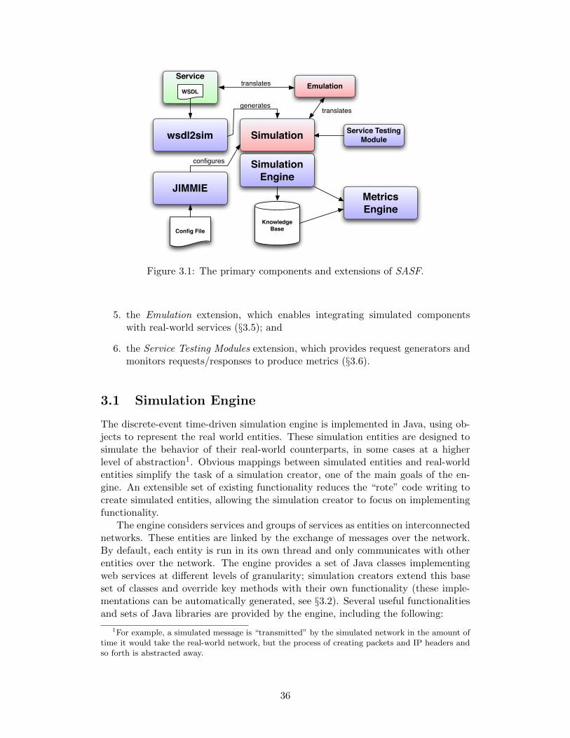
JIMMIE
wsdl2sim
Knowledge Base
Simulation Engine
Config File
Service
WSDL
Simulation
generates
configures
Metrics Engine
Emulationtranslates
translates
Service Testing Module
Figure 3.1: The primary components and extensions of SASF.
5. the Emulation extension, which enables integrating simulated componentswith real-world services (§3.5); and
6. the Service Testing Modules extension, which provides request generators andmonitors requests/responses to produce metrics (§3.6).
3.1 Simulation Engine
The discrete-event time-driven simulation engine is implemented in Java, using ob-jects to represent the real world entities. These simulation entities are designed tosimulate the behavior of their real-world counterparts, in some cases at a higherlevel of abstraction1. Obvious mappings between simulated entities and real-worldentities simplify the task of a simulation creator, one of the main goals of the en-gine. An extensible set of existing functionality reduces the “rote” code writing tocreate simulated entities, allowing the simulation creator to focus on implementingfunctionality.
The engine considers services and groups of services as entities on interconnectednetworks. These entities are linked by the exchange of messages over the network.By default, each entity is run in its own thread and only communicates with otherentities over the network. The engine provides a set of Java classes implementingweb services at different levels of granularity; simulation creators extend this baseset of classes and override key methods with their own functionality (these imple-mentations can be automatically generated, see §3.2). Several useful functionalitiesand sets of Java libraries are provided by the engine, including the following:
1For example, a simulated message is “transmitted” by the simulated network in the amount oftime it would take the real-world network, but the process of creating packets and IP headers andso forth is abstracted away.
36
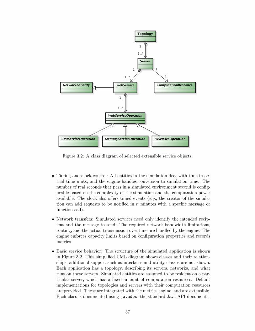
Class Diagram0 2011/02/25 powered by astah*
pkg
WebService
WebServiceOperation
1..*
1
NetworkedEntity
CPUServiceOperation MemoryServiceOperation IOServiceOperation
Server
1..*
1
ComputationResource
1
1
Topology
1..*
1
Figure 3.2: A class diagram of selected extensible service objects.
• Timing and clock control: All entities in the simulation deal with time in ac-tual time units, and the engine handles conversion to simulation time. Thenumber of real seconds that pass in a simulated environment second is config-urable based on the complexity of the simulation and the computation poweravailable. The clock also offers timed events (e.g., the creator of the simula-tion can add requests to be notified in n minutes with a specific message orfunction call).
• Network transfers: Simulated services need only identify the intended recip-ient and the message to send. The required network bandwidth limitations,routing, and the actual transmission over time are handled by the engine. Theengine enforces capacity limits based on configuration properties and recordsmetrics.
• Basic service behavior: The structure of the simulated application is shownin Figure 3.2. This simplified UML diagram shows classes and their relation-ships; additional support such as interfaces and utility classes are not shown.Each application has a topology, describing its servers, networks, and whatruns on those servers. Simulated entities are assumed to be resident on a par-ticular server, which has a fixed amount of computation resources. Defaultimplementations for topologies and servers with their computation resourcesare provided. These are integrated with the metrics engine, and are extensible.Each class is documented using javadoc, the standard Java API documenta-
37
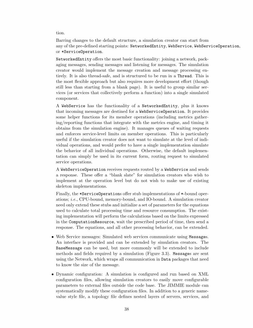
tion.
Barring changes to the default structure, a simulation creator can start fromany of the pre-defined starting points: NetworkedEntity, WebService, WebServiceOperation,or *ServiceOperation.
NetworkedEntity offers the most basic functionality: joining a network, pack-aging messages, sending messages and listening for messages. The simulationcreator would implement the message creation and message processing en-tirely. It is also thread-safe, and is structured to be run in a Thread. This isthe most flexible approach but also requires more development effort (thoughstill less than starting from a blank page). It is useful to group similar ser-vices (or services that collectively perform a function) into a single simulatedcomponent.
A WebService has the functionality of a NetworkedEntity, plus it knowsthat incoming messages are destined for a WebServiceOperation. It providessome helper functions for its member operations (including metrics gather-ing/reporting functions that integrate with the metrics engine, and timing itobtains from the simulation engine). It manages queues of waiting requestsand enforces service-level limits on member operations. This is particularlyuseful if the simulation creator does not want to simulate at the level of indi-vidual operations, and would prefer to have a single implementation simulatethe behavior of all individual operations. Otherwise, the default implemen-tation can simply be used in its current form, routing request to simulatedservice operations.
A WebServiceOperation receives requests routed by a WebService and sendsa response. These offer a “blank slate” for simulation creators who wish toimplement at the operation level but do not wish to make use of existingskeleton implementations.
Finally, the *ServiceOperations offer stub implementations of *-bound oper-ations; i.e., CPU-bound, memory-bound, and IO-bound. A simulation creatorneed only extend these stubs and initialize a set of parameters for the equationsused to calculate total processing time and resource consumption. The exist-ing implementation will perform the calculations based on the limits expressedin the ComputationResource, wait the prescribed period of time, then send aresponse. The equations, and all other processing behavior, can be extended.
• Web Service messages: Simulated web services communicate using Messages.An interface is provided and can be extended by simulation creators. TheBaseMessage can be used, but more commonly will be extended to includemethods and fields required by a simulation (Figure 3.3). Messages are sentusing the Network, which wraps all communication in Data packages that needto know the size of the message.
• Dynamic configuration: A simulation is configured and run based on XMLconfiguration files, allowing simulation creators to easily move configurableparameters to external files outside the code base. The JIMMIE module cansystematically modify these configuration files. In addition to a generic name-value style file, a topology file defines nested layers of servers, services, and
38
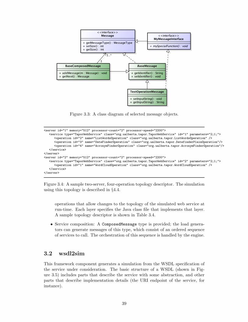
Class Diagram0 2011/03/07 powered by astah*
pkg
+ setIdentifier() : void+ getIdentifier() : String
BaseMessage
+ getSize() : int+ setSize() : int+ getMessageType() : MessageType
<<interface>>Message
+ mySpecialFunction() : void
<<interface>>MyMessageInterface
+ getInputString() : String+ setInputString() : void
TestOperationMessage
+ getNext() : Message+ addMessage(m : Message) : void
BaseComposedMessage
1..*
1
Figure 3.3: A class diagram of selected message objects.
<server id="1" memory="512" processor-count="2" processor-speed="2200">
<service type="TaporWebService" class="org.ualberta.tapor.TaporWebService" id="1" parameters="2;1;">
<operation id="2" name="ListWordsOperation" class="org.ualberta.tapor.ListWordsOperation" />
<operation id="3" name="DateFinderOperation" class="org.ualberta.tapor.DatefinderPlainOperation"/>
<operation id="4" name="AcronymFinderOperation" class="org.ualberta.tapor.AcronymFinderOperation"/>
</service>
</server>
<server id="2" memory="512" processor-count="2" processor-speed="2200">
<service type="TaporWebService" class="org.ualberta.tapor.TaporWebService" id="2" parameters="2;1;">
<operation id="1" name="WordCloudOperation" class="org.ualberta.tapor.WordCloudOperation" />
</service>
</server>
Figure 3.4: A sample two-server, four-operation topology descriptor. The simulationusing this topology is described in §4.4.
operations that allow changes to the topology of the simulated web service atrun-time. Each layer specifies the Java class file that implements that layer.A sample topology descriptor is shown in Table 3.4.
• Service composition: A ComposedMessage type is provided; the load genera-tors can generate messages of this type, which consist of an ordered sequenceof services to call. The orchestration of this sequence is handled by the engine.
3.2 wsdl2sim
This framework component generates a simulation from the WSDL specification ofthe service under consideration. The basic structure of a WSDL (shown in Fig-ure 3.5) includes parts that describe the service with some abstraction, and otherparts that describe implementation details (the URI endpoint of the service, forinstance).
39
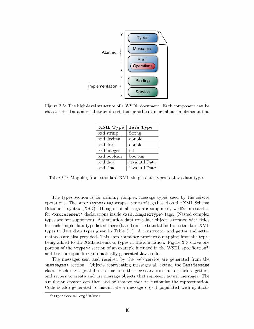
Abstract
Implementation
Types
Messages
Ports
Binding
Service
Operations
Figure 3.5: The high-level structure of a WSDL document. Each component can becharacterized as a more abstract description or as being more about implementation.
XML Type Java Type
xsd:string String
xsd:decimal double
xsd:float double
xsd:integer int
xsd:boolean boolean
xsd:date java.util.Date
xsd:time java.util.Date
Table 3.1: Mapping from standard XML simple data types to Java data types.
The types section is for defining complex message types used by the serviceoperations. The outer <types> tag wraps a series of tags based on the XML SchemaDocument syntax (XSD). Though not all tags are supported, wsdl2sim searchesfor <xsd:element> declarations inside <xsd:complexType> tags. (Nested complextypes are not supported). A simulation data container object is created with fieldsfor each simple data type listed there (based on the translation from standard XMLtypes to Java data types given in Table 3.1). A constructor and getter and settermethods are also provided. This data container provides a mapping from the typesbeing added to the XML schema to types in the simulation. Figure 3.6 shows oneportion of the <types> section of an example included in the WSDL specification2,and the corresponding automatically generated Java code.
The messages sent and received by the web service are generated from the<messages> section. Objects representing messages all extend the BaseMessage
class. Each message stub class includes the necessary constructor, fields, getters,and setters to create and use message objects that represent actual messages. Thesimulation creator can then add or remove code to customize the representation.Code is also generated to instantiate a message object populated with syntacti-
2http://www.w3.org/TR/wsdl
40
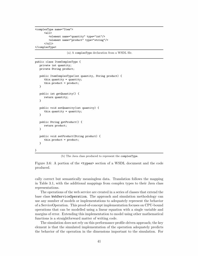
<complexType name="Item">
<all>
<element name="quantity" type="int"/>
<element name="product" type="string"/>
</all>
</complexType>
(a) A complexType declaration from a WSDL file.
public class ItemComplexType {
private int quantity;
private String product;
public ItemComplexType(int quantity, String product) {
this.quantity = quantity;
this.product = product;
}
public int getQuantity() {
return quantity;
}
public void setQuantity(int quantity) {
this.quantity = quantity;
}
public String getProduct() {
return product;
}
public void setProduct(String product) {
this.product = product;
}
}
(b) The Java class produced to represent the complexType.
Figure 3.6: A portion of the <types> section of a WSDL document and the codeproduced.
cally correct but semantically meaningless data. Translation follows the mappingin Table 3.1, with the additional mappings from complex types to their Java classrepresentations.
The operations of the web service are created in a series of classes that extend thebase class WebServiceOperation. The approach and simulation methodology canuse any number of models or implementations to adequately represent the behaviorof a ServiceOperation. This proof-of-concept implementation focuses on CPU-boundoperations that can be modelled using a linear equation with a single variable andmargins of error. Extending this implementation to model using other mathematicalfunctions is a straightforward matter of writing code.
The simulation does not rely on this performance profile-driven approach; the keyelement is that the simulated implementation of the operation adequately predictsthe behavior of the operation in the dimensions important to the simulation. For
41
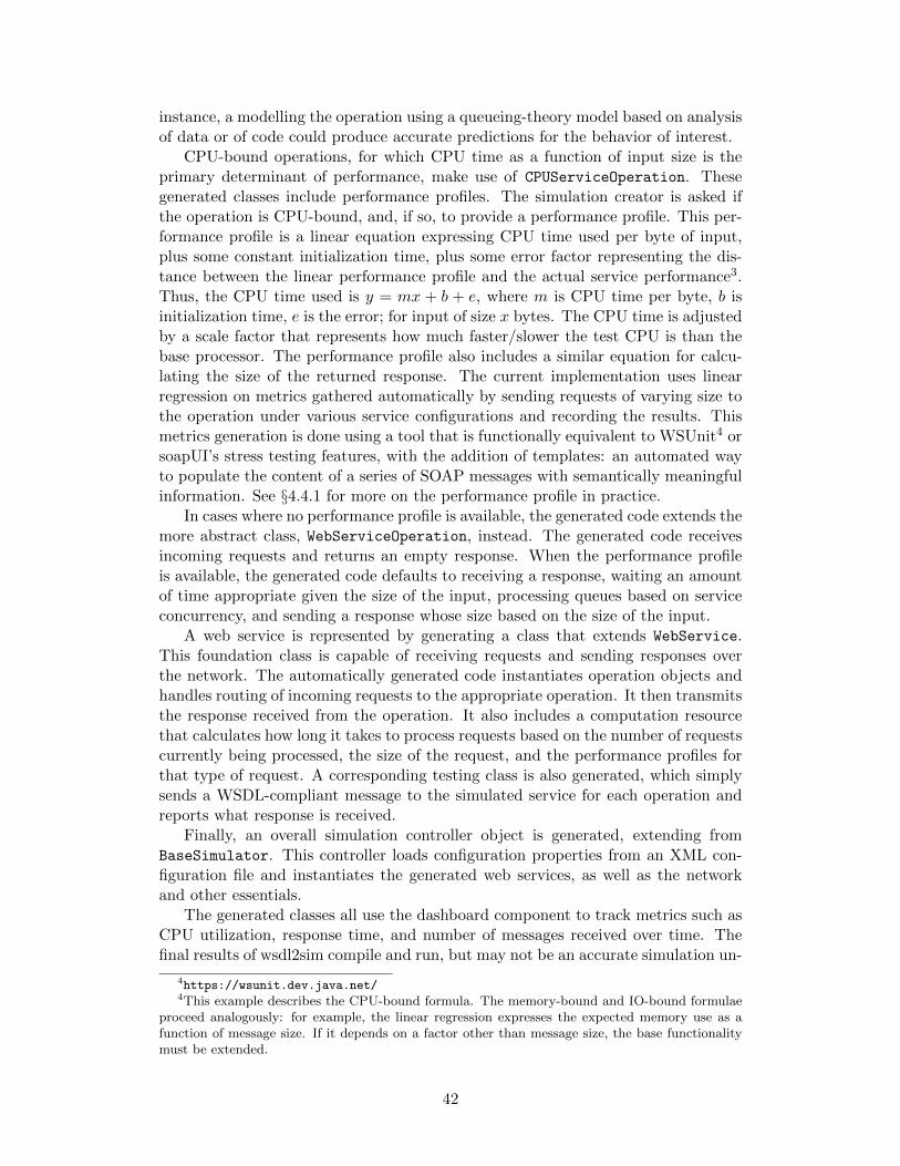
instance, a modelling the operation using a queueing-theory model based on analysisof data or of code could produce accurate predictions for the behavior of interest.
CPU-bound operations, for which CPU time as a function of input size is theprimary determinant of performance, make use of CPUServiceOperation. Thesegenerated classes include performance profiles. The simulation creator is asked ifthe operation is CPU-bound, and, if so, to provide a performance profile. This per-formance profile is a linear equation expressing CPU time used per byte of input,plus some constant initialization time, plus some error factor representing the dis-tance between the linear performance profile and the actual service performance3.Thus, the CPU time used is y = mx + b + e, where m is CPU time per byte, b isinitialization time, e is the error; for input of size x bytes. The CPU time is adjustedby a scale factor that represents how much faster/slower the test CPU is than thebase processor. The performance profile also includes a similar equation for calcu-lating the size of the returned response. The current implementation uses linearregression on metrics gathered automatically by sending requests of varying size tothe operation under various service configurations and recording the results. Thismetrics generation is done using a tool that is functionally equivalent to WSUnit4 orsoapUI’s stress testing features, with the addition of templates: an automated wayto populate the content of a series of SOAP messages with semantically meaningfulinformation. See §4.4.1 for more on the performance profile in practice.
In cases where no performance profile is available, the generated code extends themore abstract class, WebServiceOperation, instead. The generated code receivesincoming requests and returns an empty response. When the performance profileis available, the generated code defaults to receiving a response, waiting an amountof time appropriate given the size of the input, processing queues based on serviceconcurrency, and sending a response whose size based on the size of the input.
A web service is represented by generating a class that extends WebService.This foundation class is capable of receiving requests and sending responses overthe network. The automatically generated code instantiates operation objects andhandles routing of incoming requests to the appropriate operation. It then transmitsthe response received from the operation. It also includes a computation resourcethat calculates how long it takes to process requests based on the number of requestscurrently being processed, the size of the request, and the performance profiles forthat type of request. A corresponding testing class is also generated, which simplysends a WSDL-compliant message to the simulated service for each operation andreports what response is received.
Finally, an overall simulation controller object is generated, extending fromBaseSimulator. This controller loads configuration properties from an XML con-figuration file and instantiates the generated web services, as well as the networkand other essentials.
The generated classes all use the dashboard component to track metrics such asCPU utilization, response time, and number of messages received over time. Thefinal results of wsdl2sim compile and run, but may not be an accurate simulation un-
4https://wsunit.dev.java.net/4This example describes the CPU-bound formula. The memory-bound and IO-bound formulae
proceed analogously: for example, the linear regression expresses the expected memory use as afunction of message size. If it depends on a factor other than message size, the base functionalitymust be extended.
42
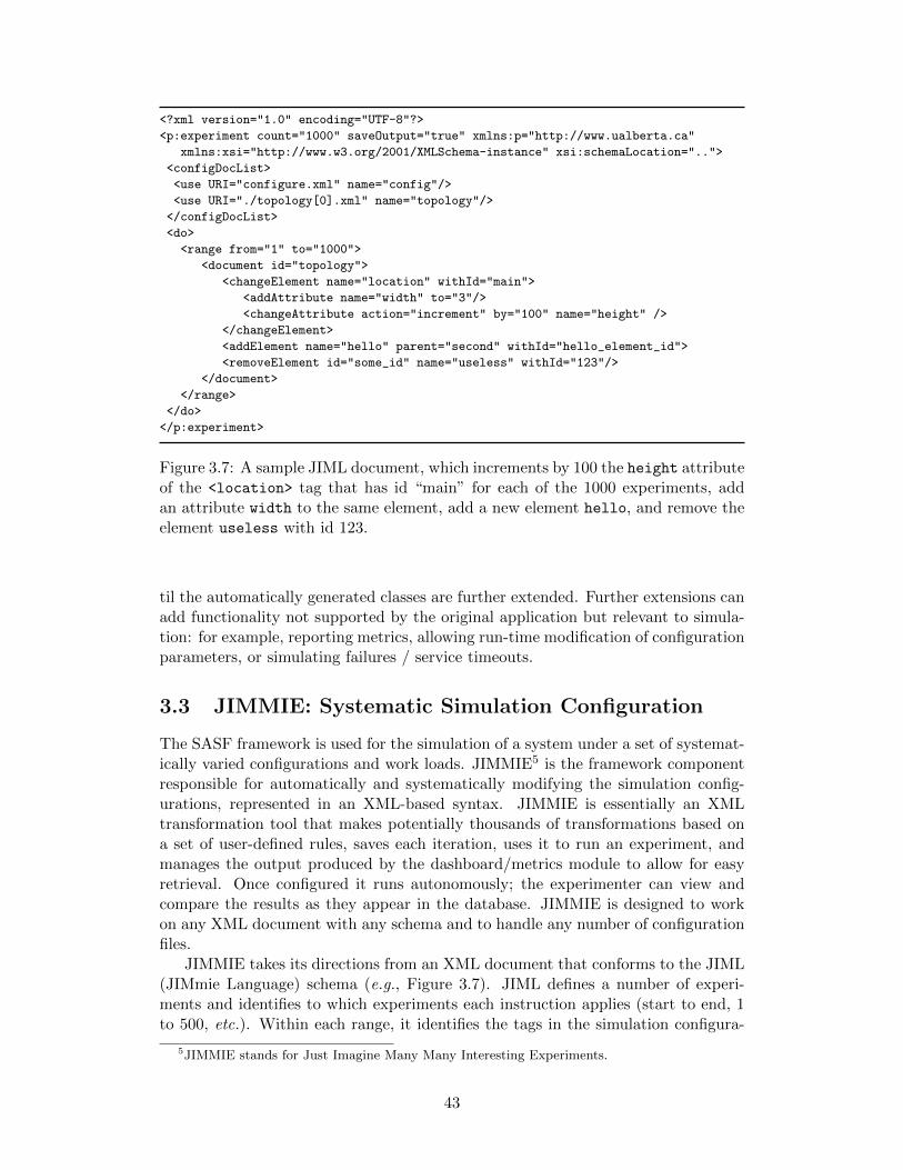
<?xml version="1.0" encoding="UTF-8"?>
<p:experiment count="1000" saveOutput="true" xmlns:p="http://www.ualberta.ca"
xmlns:xsi="http://www.w3.org/2001/XMLSchema-instance" xsi:schemaLocation="..">
<configDocList>
<use URI="configure.xml" name="config"/>
<use URI="./topology[0].xml" name="topology"/>
</configDocList>
<do>
<range from="1" to="1000">
<document id="topology">
<changeElement name="location" withId="main">
<addAttribute name="width" to="3"/>
<changeAttribute action="increment" by="100" name="height" />
</changeElement>
<addElement name="hello" parent="second" withId="hello_element_id">
<removeElement id="some_id" name="useless" withId="123"/>
</document>
</range>
</do>
</p:experiment>
Figure 3.7: A sample JIML document, which increments by 100 the height attributeof the <location> tag that has id “main” for each of the 1000 experiments, addan attribute width to the same element, add a new element hello, and remove theelement useless with id 123.
til the automatically generated classes are further extended. Further extensions canadd functionality not supported by the original application but relevant to simula-tion: for example, reporting metrics, allowing run-time modification of configurationparameters, or simulating failures / service timeouts.
3.3 JIMMIE: Systematic Simulation Configuration
The SASF framework is used for the simulation of a system under a set of systemat-ically varied configurations and work loads. JIMMIE5 is the framework componentresponsible for automatically and systematically modifying the simulation config-urations, represented in an XML-based syntax. JIMMIE is essentially an XMLtransformation tool that makes potentially thousands of transformations based ona set of user-defined rules, saves each iteration, uses it to run an experiment, andmanages the output produced by the dashboard/metrics module to allow for easyretrieval. Once configured it runs autonomously; the experimenter can view andcompare the results as they appear in the database. JIMMIE is designed to workon any XML document with any schema and to handle any number of configurationfiles.
JIMMIE takes its directions from an XML document that conforms to the JIML(JIMmie Language) schema (e.g., Figure 3.7). JIML defines a number of experi-ments and identifies to which experiments each instruction applies (start to end, 1to 500, etc.). Within each range, it identifies the tags in the simulation configura-
5JIMMIE stands for Just Imagine Many Many Interesting Experiments.
43
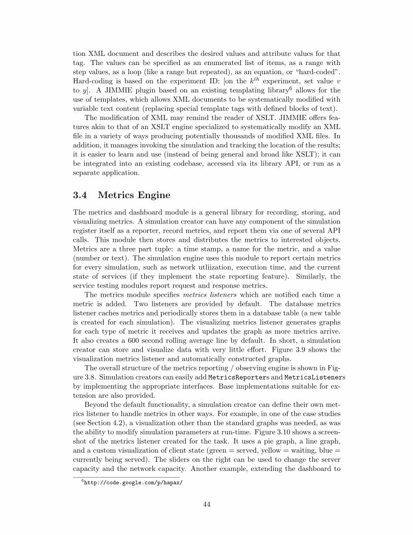
tion XML document and describes the desired values and attribute values for thattag. The values can be specified as an enumerated list of items, as a range withstep values, as a loop (like a range but repeated), as an equation, or “hard-coded”.Hard-coding is based on the experiment ID: [on the kth experiment, set value vto y]. A JIMMIE plugin based on an existing templating library6 allows for theuse of templates, which allows XML documents to be systematically modified withvariable text content (replacing special template tags with defined blocks of text).
The modification of XML may remind the reader of XSLT. JIMMIE offers fea-tures akin to that of an XSLT engine specialized to systematically modify an XMLfile in a variety of ways producing potentially thousands of modified XML files. Inaddition, it manages invoking the simulation and tracking the location of the results;it is easier to learn and use (instead of being general and broad like XSLT); it canbe integrated into an existing codebase, accessed via its library API, or run as aseparate application.
3.4 Metrics Engine
The metrics and dashboard module is a general library for recording, storing, andvisualizing metrics. A simulation creator can have any component of the simulationregister itself as a reporter, record metrics, and report them via one of several APIcalls. This module then stores and distributes the metrics to interested objects.Metrics are a three part tuple: a time stamp, a name for the metric, and a value(number or text). The simulation engine uses this module to report certain metricsfor every simulation, such as network utliization, execution time, and the currentstate of services (if they implement the state reporting feature). Similarly, theservice testing modules report request and response metrics.
The metrics module specifies metrics listeners which are notified each time ametric is added. Two listeners are provided by default. The database metricslistener caches metrics and periodically stores them in a database table (a new tableis created for each simulation). The visualizing metrics listener generates graphsfor each type of metric it receives and updates the graph as more metrics arrive.It also creates a 600 second rolling average line by default. In short, a simulationcreator can store and visualize data with very little effort. Figure 3.9 shows thevisualization metrics listener and automatically constructed graphs.
The overall structure of the metrics reporting / observing engine is shown in Fig-ure 3.8. Simulation creators can easily add MetricsReporters and MetricsListenersby implementing the appropriate interfaces. Base implementations suitable for ex-tension are also provided.
Beyond the default functionality, a simulation creator can define their own met-rics listener to handle metrics in other ways. For example, in one of the case studies(see Section 4.2), a visualization other than the standard graphs was needed, as wasthe ability to modify simulation parameters at run-time. Figure 3.10 shows a screen-shot of the metrics listener created for the task. It uses a pie graph, a line graph,and a custom visualization of client state (green = served, yellow = waiting, blue =currently being served). The sliders on the right can be used to change the servercapacity and the network capacity. Another example, extending the dashboard to
6http://code.google.com/p/hapax/
44
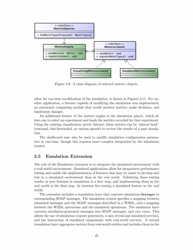
Class Diagram2 2011/03/02 powered by astah*
pkg
+ registerListener() : void+ newMetric(m : Metric) : void
MetricsEngine
+ registerMetricTypes() : void+ newMetric() : void
<<interface>>MetricsListener
VisualizingMetricsListener DatabaseMetricsListener
Metric
+ listMetricTypesProduced() : MetricTypes[]
<<interface>>MetricsReporter
Figure 3.8: A class diagram of selected metrics objects.
allow for run-time modification of the simulation, is shown in Figures 4.11. For an-other application, a listener capable of modifying the simulation was implemented:an autonomic computing module that would monitor metrics, make decisions, andimplement changes.
An additional feature of the metrics engine is the simulation player, which al-lows one to select an experiment and loads the metrics recorded for that experiment.Using the existing visualization metric listener, these metrics can be “played back”(rewound, fast-forwarded, at various speeds) to review the results of a past simula-tion.
The dashboard may also be used to modify simulation configuration parame-ters at run-time, though this requires more complex integration by the simulationcreator.
3.5 Emulation Extension
The role of the Emulation extension is to integrate the simulated environment witha real-world environment. Simulated applications allow for inexpensive performancetesting and enable the implementation of features that may be easier to develop andtest in a simulated environment than in the real world. Validating these testingresults or new features in simulation is a first step, and implementing them in thereal world is the final step. In between lies testing a simulated feature in the realworld.
The extension includes a translation layer that converts simulation Messages tocorresponding SOAP messages. The simulation creator specifies a mapping betweensimulated messages and the SOAP messages described in a WSDL, and a mappingbetween the WSDL operations and the simulated operations. The emulation layerconverts simulation-generated messages into SOAP messages, and vice versa. Thisallows the use of simulation request generators, a mix of real and simulated services,and the interaction of simulated components with real-world services. A secondtranslation layer aggregates metrics from real-world entities and includes them in the
45
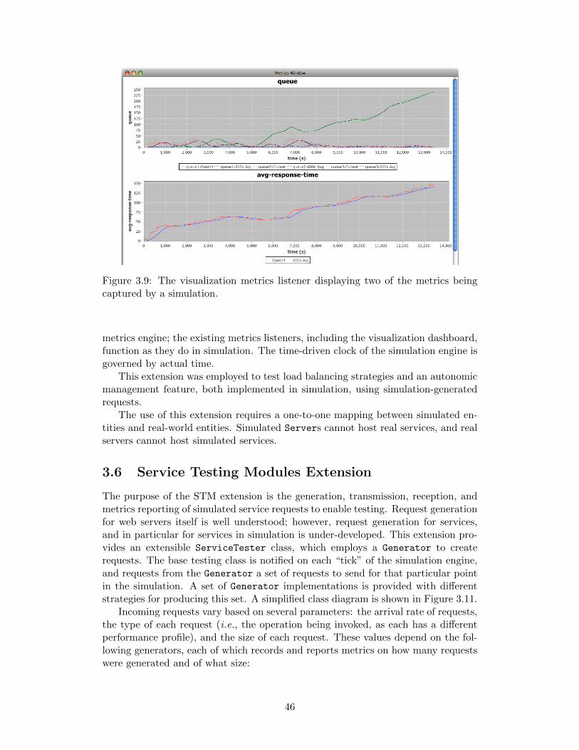
Figure 3.9: The visualization metrics listener displaying two of the metrics beingcaptured by a simulation.
metrics engine; the existing metrics listeners, including the visualization dashboard,function as they do in simulation. The time-driven clock of the simulation engine isgoverned by actual time.
This extension was employed to test load balancing strategies and an autonomicmanagement feature, both implemented in simulation, using simulation-generatedrequests.
The use of this extension requires a one-to-one mapping between simulated en-tities and real-world entities. Simulated Servers cannot host real services, and realservers cannot host simulated services.
3.6 Service Testing Modules Extension
The purpose of the STM extension is the generation, transmission, reception, andmetrics reporting of simulated service requests to enable testing. Request generationfor web servers itself is well understood; however, request generation for services,and in particular for services in simulation is under-developed. This extension pro-vides an extensible ServiceTester class, which employs a Generator to createrequests. The base testing class is notified on each “tick” of the simulation engine,and requests from the Generator a set of requests to send for that particular pointin the simulation. A set of Generator implementations is provided with differentstrategies for producing this set. A simplified class diagram is shown in Figure 3.11.
Incoming requests vary based on several parameters: the arrival rate of requests,the type of each request (i.e., the operation being invoked, as each has a differentperformance profile), and the size of each request. These values depend on the fol-lowing generators, each of which records and reports metrics on how many requestswere generated and of what size:
46
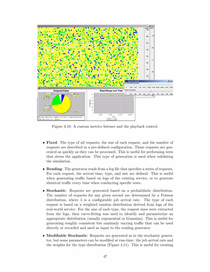
Figure 3.10: A custom metrics listener and the playback control.
• Fixed: The type of all requests, the size of each request, and the number ofrequests are described in a pre-defined configuration. These requests are gen-erated as quickly as they can be processed. This is useful for performing teststhat stress the application. This type of generation is used when validatingthe simulation.
• Reading: The generator reads from a log file that specifies a series of requests.For each request, the arrival time, type, and size are defined. This is usefulwhen generating traffic based on logs of the existing service, or to generateidentical traffic every time when conducting specific tests.
• Stochastic: Requests are generated based on a probabilistic distribution.The number of requests for any given second are determined by a Poissondistribution, where λ is a configurable job arrival rate. The type of eachrequest is based on a weighted random distribution derived from logs of thereal-world service. For the size of each type, the request sizes were extractedfrom the logs, then curve-fitting was used to identify and parameterize anappropriate distribution (usually exponential or Guassian). This is useful forgenerating roughly consistent but randomly varying traffic that can be useddirectly or recorded and used as input to the reading generator.
• Modifiable Stochastic: Requests are generated as in the stochastic genera-tor, but some parameters can be modified at run-time: the job arrival rate andthe weights for the type distribution (Figure 4.11). This is useful for creating
47
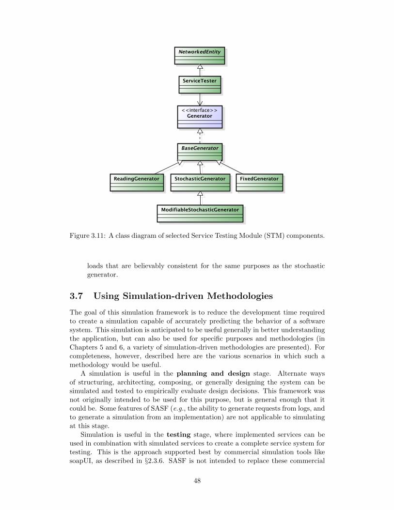
Class Diagram1 2011/02/25 powered by astah*
pkg
NetworkedEntity
ServiceTester
<<interface>>Generator
ReadingGenerator StochasticGenerator
ModifiableStochasticGenerator
FixedGenerator
BaseGenerator
Figure 3.11: A class diagram of selected Service Testing Module (STM) components.
loads that are believably consistent for the same purposes as the stochasticgenerator.
3.7 Using Simulation-driven Methodologies
The goal of this simulation framework is to reduce the development time requiredto create a simulation capable of accurately predicting the behavior of a softwaresystem. This simulation is anticipated to be useful generally in better understandingthe application, but can also be used for specific purposes and methodologies (inChapters 5 and 6, a variety of simulation-driven methodologies are presented). Forcompleteness, however, described here are the various scenarios in which such amethodology would be useful.
A simulation is useful in the planning and design stage. Alternate waysof structuring, architecting, composing, or generally designing the system can besimulated and tested to empirically evaluate design decisions. This framework wasnot originally intended to be used for this purpose, but is general enough that itcould be. Some features of SASF (e.g., the ability to generate requests from logs, andto generate a simulation from an implementation) are not applicable to simulatingat this stage.
Simulation is useful in the testing stage, where implemented services can beused in combination with simulated services to create a complete service system fortesting. This is the approach supported best by commercial simulation tools likesoapUI, as described in §2.3.6. SASF is not intended to replace these commercial
48
tools, but does offer integration between simulated and real-world services that couldbe used for this purpose.
One key area of applicability addressed here is the pre-deployment stage. Onceall of the services are implemented, a simulation can be created and used to createan appropriate deployment for the service system. Supporting the process of betterunderstanding, and systematically analyzing, an implemented service system is oneof the primary uses of simulation contemplated in this work. This is addressed in§4.2 and Chapter 5.
The second primary use of simulation in this dissertation is post-deploymentand run-time. After deployment, the simulation can be improved using the SASFtools by capturing more accurate performance profiles and logs of actual requests.Alternative configurations can be attempted in simulation to improve some aspectof the service system (here, primarily the performance). Off-line simulation canreason about the service system without interfering with it. This approach is usedexclusively in Chapter 6, and in tandem with pre-deployment simulation in Chap-ter 5.
3.8 Known Issues and Threats to Validity
The prototype of SASF is a proof-of-concept and has a number of limitations, someof which have already been mentioned.
The currently implemented CPU-bound operations, on which the automatic gen-eration depends, require a performance profile that is O(n) in time complexity, wheren is the size of the input. To support service operations with different performanceprofiles, the existing library would have to be extended. This is a matter of writingcode; conceptually, the same approach applies. The methodology - curve-fitting toa variety of metrics produced by load-testing the service - still applies, but is notyet implemented.
Complex services, particularly more complex service compositions, will still re-quire hand-coding, though less than would be required without a starting point.Support for composed messages is available for simple sequences, but more complexcompositions - conditionals, loops, parallel processing - are not yet implemented inthe framework. A simulation creator would have to provide a composition engineappropriate for their needs.
The wsdl2sim is mainly useful when considering a one-to-one simulation, whereevery operation in the web service has a corresponding object in the simulation.If a higher level of abstraction is required, its usefulness is limited. It is limitedto only CPU-bound operations, though the automatically generated code can bemodified to extend other service operation simulation templates. It also requires arequest-response web service. Chapter 4 illustrates creating a simulation both withand without using automatic generation.
No one other than the author and those who helped implement the simulationframework have used it to simulate applications; no user study of its usability forproducing simulated services has been conducted. Details of how to create a sim-ulation and important metrics like lines of code manually written are presented inChapter 4, where it is clear that less work is required when using SASF. The exactimprovement is not quantified. It should be noted that while this is reported as a
49
threat to validity, this level of evaluation actually exceeds current practice in thearea.
3.9 Summary
This chapter introduced SASF, a novel simulation framework for services-orientedsoftware systems. SASF is built around extensible libraries for common web servicefunctionality that offer more features than the current state of the art. Develop-ment effort is reduced using automatic generation of basic simulations from existingdata about the service: from the services WSDL and a performance profile, an exe-cutable simulation is generated automatically, ready for extension and enhancement.The basic generated simulation can accurately replicate the performance character-istics of a real service; existing solutions focus on composition issues and not on aminute-by-minute replication of performance metrics. A narrative of the predictedperformance of a simulation can be produced using the extensible and flexible met-rics gathering support system with its own API, which out-of-the-box is capable ofvisualizing, recording, and playing back metrics generated during a simulation.
SASF also offers the ability to interact with a running simulation, including notjust the usual user interface, but also an API so both the simulation componentsand external applications can modify configuration parameters during simulationexecution. It can integrate simulated components with real-world components bytranslating requests and messages from the simulated environment to a real-worldenvironment. It can generate requests based on real request logs or stochastic dis-tributions modelled on known request patterns. Finally, JIMMIE is an innovativelanguage and tool to run systematically modified simulations in sequence or parallelto generate data.
These contributions are compared to the current state of the art in §2.3.7; SASFmeets or exceeds the state of the art in all areas.
SASF is used to generate, test, and validate simulations in Chapter 4. Thesimulated versions are validated against their real-world counterparts and prove toproduce the same performance results.
50
Chapter 4
Simulating Service OrientedApplications
Chapter Contents
4.1 Tivoli Provisioning Manager . . . . . 52
4.1.1 Executing Jobs using the SDI . 54
4.1.2 Capacity Planning for TPM . . 55
4.2 Simulating TPM . . . . . . . . . . . 57
4.2.1 Validation . . . . . . . . . . . . 60
4.2.2 Known Issues and Threats toValidity . . . . . . . . . . . . . 61
4.3 Text Analysis Portal for Research . . 63
4.3.1 TAPoRware 2.0 . . . . . . . . . 64
4.4 Simulating TAPoRware . . . . . . . 64
4.4.1 Building Performance Profiles . 65
4.4.2 Generating and Extending Code 66
4.4.3 Validation . . . . . . . . . . . . 67
4.4.4 Systematic Simulation . . . . . 70
4.4.5 Known Issues and Threats toValidity . . . . . . . . . . . . . 71
4.5 Summary . . . . . . . . . . . . . . . 71
This chapter demonstrates the util-ity of the services-aware simulationframework described in Chapter 3, bycreating simulations for two service-oriented systems. Those systems, andthe details of the simulation approach,are described in this chapter. One sim-ulated system will be used as a test bedfor additional simulation-related toolsand methodologies in Chapters 5 and 6.
The first case study is a componentof a proprietary enterprise-level sys-tem that includes SOA-based interfaces,Tivoli Provisioning Manager (TPM). Itsfocus is on the distribution of data toa large set of endpoints using a dis-tributed architecture (potentially geo-graphically distributed). It is simulatedat a higher level of abstraction withoutusing the automatic simulation genera-tion feature; referring back to the simulation engine (§3.1), the least amount oflibrary support (NetworkedEntity) is used. Instead of a one-to-one mapping ofservice operations to simulation objects, a set of composed or related services thatimplement a set of features is simulated as a single simulation object. This show-cases the ability to simulate a complex application at an abstracted level, where aset of web services is grouped into a virtual component and a series of messages intoa virtual communications group. This higher-level groups are then the simulatedobjects. TPM is introduced in §4.1; its simulation is described in §4.2.
The second is a text-analysis tool that provides a public web services inter-face, TAPoRware, the back-end support to the Text Analysis Portal for Research(TAPoR). Its primary focus is on data processing (CPU-bound), with the move-ment of data being a secondary but still important concern. It is simulated using
51
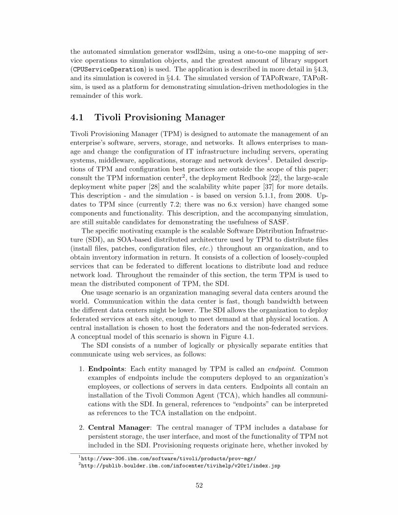
the automated simulation generator wsdl2sim, using a one-to-one mapping of ser-vice operations to simulation objects, and the greatest amount of library support(CPUServiceOperation) is used. The application is described in more detail in §4.3,and its simulation is covered in §4.4. The simulated version of TAPoRware, TAPoR-sim, is used as a platform for demonstrating simulation-driven methodologies in theremainder of this work.
4.1 Tivoli Provisioning Manager
Tivoli Provisioning Manager (TPM) is designed to automate the management of anenterprise’s software, servers, storage, and networks. It allows enterprises to man-age and change the configuration of IT infrastructure including servers, operatingsystems, middleware, applications, storage and network devices1. Detailed descrip-tions of TPM and configuration best practices are outside the scope of this paper;consult the TPM information center2, the deployment Redbook [22], the large-scaledeployment white paper [28] and the scalability white paper [37] for more details.This description - and the simulation - is based on version 5.1.1, from 2008. Up-dates to TPM since (currently 7.2; there was no 6.x version) have changed somecomponents and functionality. This description, and the accompanying simulation,are still suitable candidates for demonstrating the usefulness of SASF.
The specific motivating example is the scalable Software Distribution Infrastruc-ture (SDI), an SOA-based distributed architecture used by TPM to distribute files(install files, patches, configuration files, etc.) throughout an organization, and toobtain inventory information in return. It consists of a collection of loosely-coupledservices that can be federated to different locations to distribute load and reducenetwork load. Throughout the remainder of this section, the term TPM is used tomean the distributed component of TPM, the SDI.
One usage scenario is an organization managing several data centers around theworld. Communication within the data center is fast, though bandwidth betweenthe different data centers might be lower. The SDI allows the organization to deployfederated services at each site, enough to meet demand at that physical location. Acentral installation is chosen to host the federators and the non-federated services.A conceptual model of this scenario is shown in Figure 4.1.
The SDI consists of a number of logically or physically separate entities thatcommunicate using web services, as follows:
1. Endpoints: Each entity managed by TPM is called an endpoint. Commonexamples of endpoints include the computers deployed to an organization’semployees, or collections of servers in data centers. Endpoints all contain aninstallation of the Tivoli Common Agent (TCA), which handles all communi-cations with the SDI. In general, references to “endpoints” can be interpretedas references to the TCA installation on the endpoint.
2. Central Manager: The central manager of TPM includes a database forpersistent storage, the user interface, and most of the functionality of TPM notincluded in the SDI. Provisioning requests originate here, whether invoked by
1http://www-306.ibm.com/software/tivoli/products/prov-mgr/2http://publib.boulder.ibm.com/infocenter/tivihelp/v20r1/index.jsp
52
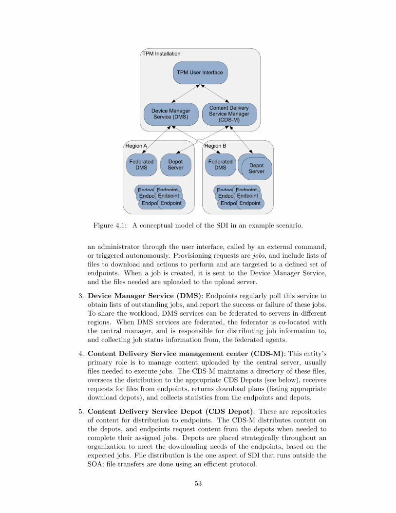
TPM Installation
Region A
Device Manager Service (DMS)
Content Delivery Service Manager
(CDS-M)
Federated DMS
Depot Server
Region B
Federated DMS
Depot ServerDepot
Server
TPM User Interface
EndpointEndpointEndpoint
EndpointEndpointEndpoint
EndpointEndpointEndpoint
EndpointEndpointEndpoint
Figure 4.1: A conceptual model of the SDI in an example scenario.
an administrator through the user interface, called by an external command,or triggered autonomously. Provisioning requests are jobs, and include lists offiles to download and actions to perform and are targeted to a defined set ofendpoints. When a job is created, it is sent to the Device Manager Service,and the files needed are uploaded to the upload server.
3. Device Manager Service (DMS): Endpoints regularly poll this service toobtain lists of outstanding jobs, and report the success or failure of these jobs.To share the workload, DMS services can be federated to servers in differentregions. When DMS services are federated, the federator is co-located withthe central manager, and is responsible for distributing job information to,and collecting job status information from, the federated agents.
4. Content Delivery Service management center (CDS-M): This entity’sprimary role is to manage content uploaded by the central server, usuallyfiles needed to execute jobs. The CDS-M maintains a directory of these files,oversees the distribution to the appropriate CDS Depots (see below), receivesrequests for files from endpoints, returns download plans (listing appropriatedownload depots), and collects statistics from the endpoints and depots.
5. Content Delivery Service Depot (CDS Depot): These are repositoriesof content for distribution to endpoints. The CDS-M distributes content onthe depots, and endpoints request content from the depots when needed tocomplete their assigned jobs. Depots are placed strategically throughout anorganization to meet the downloading needs of the endpoints, based on theexpected jobs. File distribution is the one aspect of SDI that runs outside theSOA; file transfers are done using an efficient protocol.
53
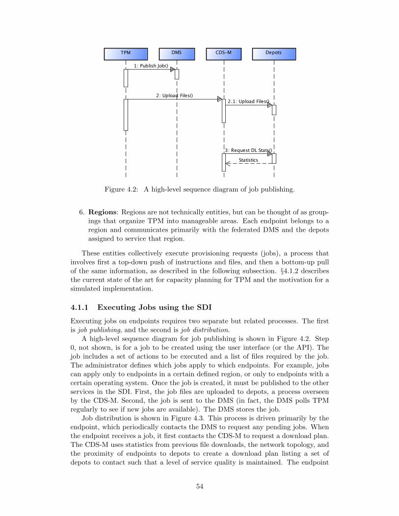
Sequence Diagram1 2011/03/03 powered by astah*
Sequence Diagram1sd
TPM DepotsCDS-MDMS
1: Publish Job()
2: Upload Files()2.1: Upload Files()
3: Request DL Stats()
Statistics
Figure 4.2: A high-level sequence diagram of job publishing.
6. Regions: Regions are not technically entities, but can be thought of as group-ings that organize TPM into manageable areas. Each endpoint belongs to aregion and communicates primarily with the federated DMS and the depotsassigned to service that region.
These entities collectively execute provisioning requests (jobs), a process thatinvolves first a top-down push of instructions and files, and then a bottom-up pullof the same information, as described in the following subsection. §4.1.2 describesthe current state of the art for capacity planning for TPM and the motivation for asimulated implementation.
4.1.1 Executing Jobs using the SDI
Executing jobs on endpoints requires two separate but related processes. The firstis job publishing, and the second is job distribution.
A high-level sequence diagram for job publishing is shown in Figure 4.2. Step0, not shown, is for a job to be created using the user interface (or the API). Thejob includes a set of actions to be executed and a list of files required by the job.The administrator defines which jobs apply to which endpoints. For example, jobscan apply only to endpoints in a certain defined region, or only to endpoints with acertain operating system. Once the job is created, it must be published to the otherservices in the SDI. First, the job files are uploaded to depots, a process overseenby the CDS-M. Second, the job is sent to the DMS (in fact, the DMS polls TPMregularly to see if new jobs are available). The DMS stores the job.
Job distribution is shown in Figure 4.3. This process is driven primarily by theendpoint, which periodically contacts the DMS to request any pending jobs. Whenthe endpoint receives a job, it first contacts the CDS-M to request a download plan.The CDS-M uses statistics from previous file downloads, the network topology, andthe proximity of endpoints to depots to create a download plan listing a set ofdepots to contact such that a level of service quality is maintained. The endpoint
54
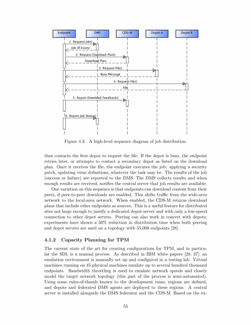
Sequence Diagram0 2011/03/03 powered by astah*
Sequence Diagram0sd
Depot BDepot ACDS-MDMSEndpoint
1: Request Job()
Job (If Exists)
2: Request Download Plan()
Download Plan
3: Request File()
Busy Message
4: Request File()
File
5: Report Download Feedback()
6: Report Job Status()
Figure 4.3: A high-level sequence diagram of job distribution.
then contacts the first depot to request the file. If the depot is busy, the endpointretries later, or attempts to contact a secondary depot as listed on the downloadplan. Once it receives the file, the endpoint executes the job: applying a securitypatch, updating virus definitions, whatever the task may be. The results of the job(success or failure) are reported to the DMS. The DMS collects results and whenenough results are received, notifies the central server that job results are available.
One variation on this sequence is that endpoints can download content from theirpeers, if peer-to-peer downloads are enabled. This shifts traffic from the wide-areanetwork to the local-area network. When enabled, the CDS-M returns downloadplans that include other endpoints as sources. This is a useful feature for distributedsites not large enough to justify a dedicated depot server and with only a low-speedconnection to other depot servers. Peering can also work in concert with depots;experiments have shown a 50% reduction in distribution time when both peeringand depot servers are used on a topology with 55,000 endpoints [28].
4.1.2 Capacity Planning for TPM
The current state of the art for creating configurations for TPM, and in particu-lar the SDI, is a manual process. As described in IBM white papers [28, 37], anemulation environment is manually set up and configured in a testing lab. Virtualmachines running on 45 physical machines emulate up to several hundred thousandendpoints. Bandwidth throttling is used to emulate network speeds and closelymodel the target network topology (this part of the process is semi-automated).Using some rules-of-thumb known to the development team, regions are defined,and depots and federated DMS agents are deployed to these regions. A centralserver is installed alongside the DMS federator and the CDS-M. Based on the ex-
55
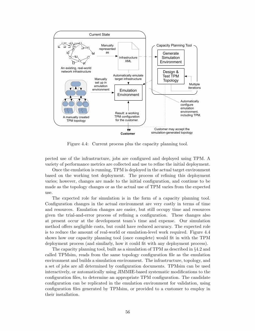
Infrastructure XML
Manually represented
as
An existing, real-world network infrastructure
A manually createdTPM topology
Emulation Environment
Automatically emulate target infrastructureManually
set up in emulation
environment
Current State
Capacity Planning Tool
Automatically configure emulation environment, including TPM.
Generate Simulation
Environment
Design & Test TPM Topology
Multiple iterations
Customer may accept the simulation-generated topology Customer
Result: a working TPM configuration for the customer.
Figure 4.4: Current process plus the capacity planning tool.
pected use of the infrastructure, jobs are configured and deployed using TPM. Avariety of performance metrics are collected and use to refine the initial deployment.
Once the emulation is running, TPM is deployed in the actual target environmentbased on the working test deployment. The process of refining this deploymentvaries; however, changes are made to the initial configuration, and continue to bemade as the topology changes or as the actual use of TPM varies from the expecteduse.
The expected role for simulation is in the form of a capacity planning tool.Configuration changes in the actual environment are very costly in terms of timeand resources. Emulation changes are easier, but still occupy time and resourcesgiven the trial-and-error process of refining a configuration. These changes alsoat present occur at the development team’s time and expense. Our simulationmethod offers negligible costs, but could have reduced accuracy. The expected roleis to reduce the amount of real-world or emulation-level work required. Figure 4.4shows how our capacity planning tool (once complete) would fit in with the TPMdeployment process (and similarly, how it could fit with any deployment process).
The capacity planning tool, built as a simulation of TPM as described in §4.2 andcalled TPMsim, reads from the same topology configuration file as the emulationenvironment and builds a simulation environment. The infrastructure, topology, anda set of jobs are all determined by configuration documents. TPMsim can be usedinteractively, or automatically using JIMMIE-based systematic modifications to theconfiguration files, to determine an appropriate TPM configuration. The candidateconfiguration can be replicated in the emulation environment for validation, usingconfiguration files generated by TPMsim, or provided to a customer to employ intheir installation.
56
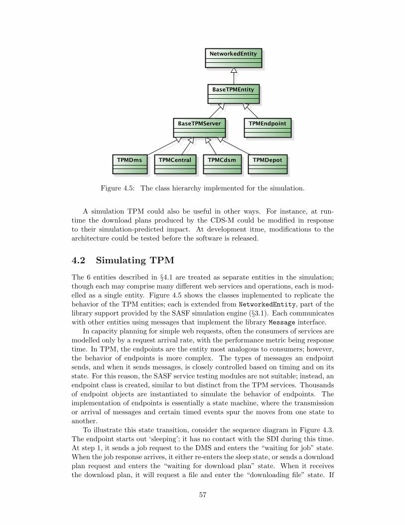
Class Diagram0 2011/03/03 powered by astah*
pkg
NetworkedEntity
BaseTPMEntity
BaseTPMServer TPMEndpoint
TPMDms TPMCentral TPMCdsm TPMDepot
Figure 4.5: The class hierarchy implemented for the simulation.
A simulation TPM could also be useful in other ways. For instance, at run-time the download plans produced by the CDS-M could be modified in responseto their simulation-predicted impact. At development itme, modifications to thearchitecture could be tested before the software is released.
4.2 Simulating TPM
The 6 entities described in §4.1 are treated as separate entities in the simulation;though each may comprise many different web services and operations, each is mod-elled as a single entity. Figure 4.5 shows the classes implemented to replicate thebehavior of the TPM entities; each is extended from NetworkedEntity, part of thelibrary support provided by the SASF simulation engine (§3.1). Each communicateswith other entities using messages that implement the library Message interface.
In capacity planning for simple web requests, often the consumers of services aremodelled only by a request arrival rate, with the performance metric being responsetime. In TPM, the endpoints are the entity most analogous to consumers; however,the behavior of endpoints is more complex. The types of messages an endpointsends, and when it sends messages, is closely controlled based on timing and on itsstate. For this reason, the SASF service testing modules are not suitable; instead, anendpoint class is created, similar to but distinct from the TPM services. Thousandsof endpoint objects are instantiated to simulate the behavior of endpoints. Theimplementation of endpoints is essentially a state machine, where the transmissionor arrival of messages and certain timed events spur the moves from one state toanother.
To illustrate this state transition, consider the sequence diagram in Figure 4.3.The endpoint starts out ‘sleeping’; it has no contact with the SDI during this time.At step 1, it sends a job request to the DMS and enters the “waiting for job” state.When the job response arrives, it either re-enters the sleep state, or sends a downloadplan request and enters the “waiting for download plan” state. When it receivesthe download plan, it will request a file and enter the “downloading file” state. If
57
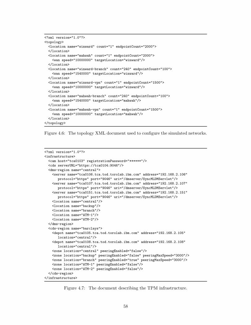
<?xml version="1.0"?>
<topology>
<location name="winward" count="1" endpointCount="2000">
</location>
<location name="mahwah" count="1" endpointCount="2000">
<wan speed="10000000" targetLocation="winward"/>
</location>
<location name="winward-branch" count="240" endpointCount="100">
<wan speed="1540000" targetLocation="winward"/>
</location>
<location name="winward-vpn" count="1" endpointCount="1500">
<wan speed="10000000" targetLocation="winward"/>
</location>
<location name="mahwah-branch" count="240" endpointCount="100">
<wan speed="1540000" targetLocation="mahwah"/>
</location>
<location name="mahwah-vpn" count="1" endpointCount="1500">
<wan speed="10000000" targetLocation="mahwah"/>
</location>
</topology>
Figure 4.6: The topology XML document used to configure the simulated networks.
<?xml version="1.0"?>
<infrastructure>
<cam host="tca0103" registrationPassword="******"/>
<cds serverURL="https://tca0104:9046"/>
<dms-region name="central">
<server name="tca0106.tca.tod.torolab.ibm.com" address="192.168.2.106"
protocol="https" port="9046" uri="/dmserver/SyncMLDMServlet"/>
<server name="tca0107.tca.tod.torolab.ibm.com" address="192.168.2.107"
protocol="https" port="9046" uri="/dmserver/SyncMLDMServlet"/>
<server name="tca0151.tca.tod.torolab.ibm.com" address="192.168.2.151"
protocol="https" port="9046" uri="/dmserver/SyncMLDMServlet"/>
<location name="central"/>
<location name="backup"/>
<location name="branch"/>
<location name="ATM-1"/>
<location name="ATM-2"/>
</dms-region>
<cds-region name="barclays">
<depot name="tca0105.tca.tod.torolab.ibm.com" address="192.168.2.105"
location="central"/>
<depot name="tca0108.tca.tod.torolab.ibm.com" address="192.168.2.108"
location="central"/>
<zone location="central" peeringEnabled="false"/>
<zone location="backup" peeringEnabled="false" peeringMaxSpeed="3000"/>
<zone location="branch" peeringEnabled="true" peeringMaxSpeed="3000"/>
<zone location="ATM-1" peeringEnabled="false"/>
<zone location="ATM-2" peeringEnabled="false"/>
</cds-region>
</infrastructure>
Figure 4.7: The document describing the TPM infrastructure.
58
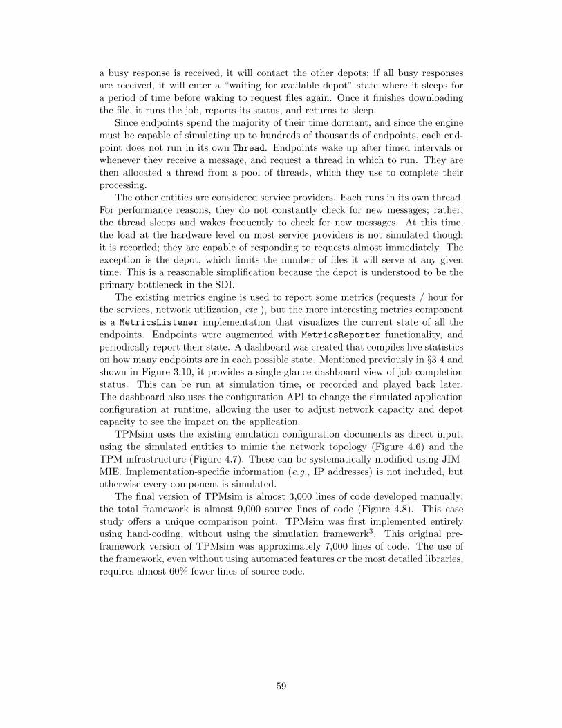
a busy response is received, it will contact the other depots; if all busy responsesare received, it will enter a “waiting for available depot” state where it sleeps fora period of time before waking to request files again. Once it finishes downloadingthe file, it runs the job, reports its status, and returns to sleep.
Since endpoints spend the majority of their time dormant, and since the enginemust be capable of simulating up to hundreds of thousands of endpoints, each end-point does not run in its own Thread. Endpoints wake up after timed intervals orwhenever they receive a message, and request a thread in which to run. They arethen allocated a thread from a pool of threads, which they use to complete theirprocessing.
The other entities are considered service providers. Each runs in its own thread.For performance reasons, they do not constantly check for new messages; rather,the thread sleeps and wakes frequently to check for new messages. At this time,the load at the hardware level on most service providers is not simulated thoughit is recorded; they are capable of responding to requests almost immediately. Theexception is the depot, which limits the number of files it will serve at any giventime. This is a reasonable simplification because the depot is understood to be theprimary bottleneck in the SDI.
The existing metrics engine is used to report some metrics (requests / hour forthe services, network utilization, etc.), but the more interesting metrics componentis a MetricsListener implementation that visualizes the current state of all theendpoints. Endpoints were augmented with MetricsReporter functionality, andperiodically report their state. A dashboard was created that compiles live statisticson how many endpoints are in each possible state. Mentioned previously in §3.4 andshown in Figure 3.10, it provides a single-glance dashboard view of job completionstatus. This can be run at simulation time, or recorded and played back later.The dashboard also uses the configuration API to change the simulated applicationconfiguration at runtime, allowing the user to adjust network capacity and depotcapacity to see the impact on the application.
TPMsim uses the existing emulation configuration documents as direct input,using the simulated entities to mimic the network topology (Figure 4.6) and theTPM infrastructure (Figure 4.7). These can be systematically modified using JIM-MIE. Implementation-specific information (e.g., IP addresses) is not included, butotherwise every component is simulated.
The final version of TPMsim is almost 3,000 lines of code developed manually;the total framework is almost 9,000 source lines of code (Figure 4.8). This casestudy offers a unique comparison point. TPMsim was first implemented entirelyusing hand-coding, without using the simulation framework3. This original pre-framework version of TPMsim was approximately 7,000 lines of code. The use ofthe framework, even without using automated features or the most detailed libraries,requires almost 60% fewer lines of source code.
59
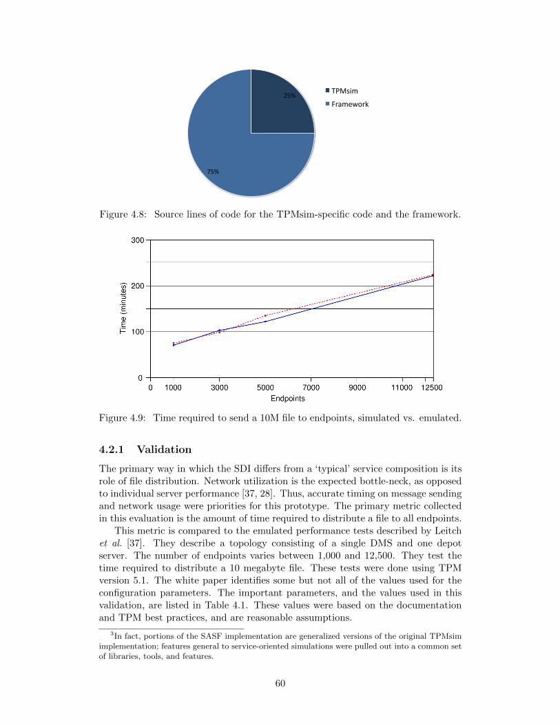
25%
75%
TPMsim
Framework
Figure 4.8: Source lines of code for the TPMsim-specific code and the framework.
Figure 4.9: Time required to send a 10M file to endpoints, simulated vs. emulated.
4.2.1 Validation
The primary way in which the SDI differs from a ‘typical’ service composition is itsrole of file distribution. Network utilization is the expected bottle-neck, as opposedto individual server performance [37, 28]. Thus, accurate timing on message sendingand network usage were priorities for this prototype. The primary metric collectedin this evaluation is the amount of time required to distribute a file to all endpoints.
This metric is compared to the emulated performance tests described by Leitchet al. [37]. They describe a topology consisting of a single DMS and one depotserver. The number of endpoints varies between 1,000 and 12,500. They test thetime required to distribute a 10 megabyte file. These tests were done using TPMversion 5.1. The white paper identifies some but not all of the values used for theconfiguration parameters. The important parameters, and the values used in thisvalidation, are listed in Table 4.1. These values were based on the documentationand TPM best practices, and are reasonable assumptions.
3In fact, portions of the SASF implementation are generalized versions of the original TPMsimimplementation; features general to service-oriented simulations were pulled out into a common setof libraries, tools, and features.
60
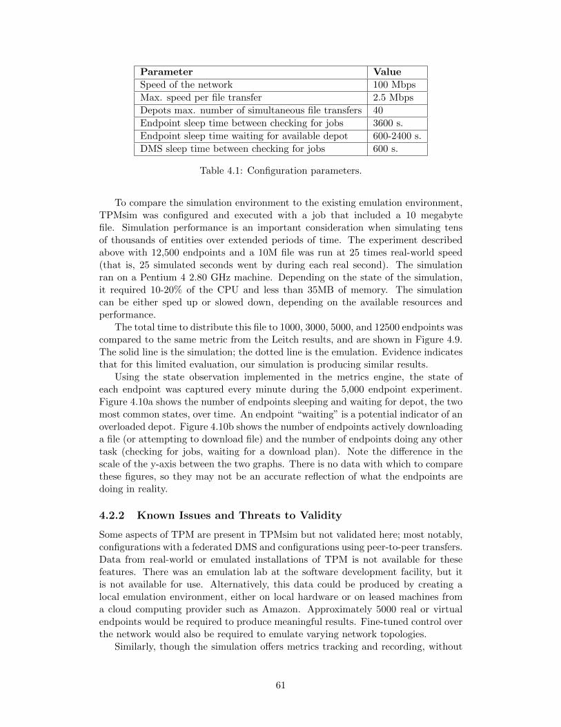
Parameter Value
Speed of the network 100 Mbps
Max. speed per file transfer 2.5 Mbps
Depots max. number of simultaneous file transfers 40
Endpoint sleep time between checking for jobs 3600 s.
Endpoint sleep time waiting for available depot 600-2400 s.
DMS sleep time between checking for jobs 600 s.
Table 4.1: Configuration parameters.
To compare the simulation environment to the existing emulation environment,TPMsim was configured and executed with a job that included a 10 megabytefile. Simulation performance is an important consideration when simulating tensof thousands of entities over extended periods of time. The experiment describedabove with 12,500 endpoints and a 10M file was run at 25 times real-world speed(that is, 25 simulated seconds went by during each real second). The simulationran on a Pentium 4 2.80 GHz machine. Depending on the state of the simulation,it required 10-20% of the CPU and less than 35MB of memory. The simulationcan be either sped up or slowed down, depending on the available resources andperformance.
The total time to distribute this file to 1000, 3000, 5000, and 12500 endpoints wascompared to the same metric from the Leitch results, and are shown in Figure 4.9.The solid line is the simulation; the dotted line is the emulation. Evidence indicatesthat for this limited evaluation, our simulation is producing similar results.
Using the state observation implemented in the metrics engine, the state ofeach endpoint was captured every minute during the 5,000 endpoint experiment.Figure 4.10a shows the number of endpoints sleeping and waiting for depot, the twomost common states, over time. An endpoint “waiting” is a potential indicator of anoverloaded depot. Figure 4.10b shows the number of endpoints actively downloadinga file (or attempting to download file) and the number of endpoints doing any othertask (checking for jobs, waiting for a download plan). Note the difference in thescale of the y-axis between the two graphs. There is no data with which to comparethese figures, so they may not be an accurate reflection of what the endpoints aredoing in reality.
4.2.2 Known Issues and Threats to Validity
Some aspects of TPM are present in TPMsim but not validated here; most notably,configurations with a federated DMS and configurations using peer-to-peer transfers.Data from real-world or emulated installations of TPM is not available for thesefeatures. There was an emulation lab at the software development facility, but itis not available for use. Alternatively, this data could be produced by creating alocal emulation environment, either on local hardware or on leased machines froma cloud computing provider such as Amazon. Approximately 5000 real or virtualendpoints would be required to produce meaningful results. Fine-tuned control overthe network would also be required to emulate varying network topologies.
Similarly, though the simulation offers metrics tracking and recording, without
61
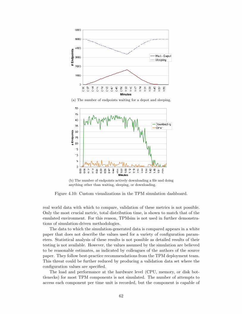
(a) The number of endpoints waiting for a depot and sleeping.
(b) The number of endpoints actively downloading a file and doinganything other than waiting, sleeping, or downloading.
Figure 4.10: Custom visualizations in the TPM simulation dashboard.
real world data with which to compare, validation of these metrics is not possible.Only the most crucial metric, total distribution time, is shown to match that of theemulated environment. For this reason, TPMsim is not used in further demonstra-tions of simulation-driven methodologies.
The data to which the simulation-generated data is compared appears in a whitepaper that does not describe the values used for a variety of configuration param-eters. Statistical analysis of these results is not possible as detailed results of theirtesting is not available. However, the values assumed by the simulation are believedto be reasonable estimates, as indicated by colleagues of the authors of the sourcepaper. They follow best-practice recommendations from the TPM deployment team.This threat could be further reduced by producing a validation data set where theconfiguration values are specified.
The load and performance at the hardware level (CPU, memory, or disk bot-tlenecks) for most TPM components is not simulated. The number of attempts toaccess each component per time unit is recorded, but the component is capable of
62
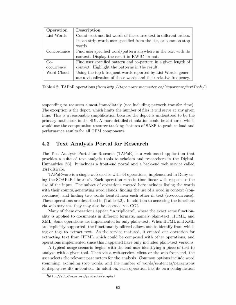
Operation Description
List Words Count, sort and list words of the source text in different orders.It can strip words user specified from the list, or common stopwords.
Concordance Find user specified word/pattern anywhere in the text with itscontext. Display the result in KWIC format.
Co-occurrence
Find user specified pattern and co-pattern in a given length ofcontext. Highlight the patterns in the result.
Word Cloud Using the top k frequent words reported by List Words, gener-ate a visualization of those words and their relative frequency.
Table 4.2: TAPoR operations (from http://taporware.mcmaster.ca/˜taporware/textTools/ )
responding to requests almost immediately (not including network transfer time).The exception is the depot, which limits the number of files it will serve at any giventime. This is a reasonable simplification because the depot is understood to be theprimary bottleneck in the SDI. A more detailed simulation could be authored whichwould use the computation resource tracking features of SASF to produce load andperformance results for all TPM components.
4.3 Text Analysis Portal for Research
The Text Analysis Portal for Research (TAPoR) is a web-based application thatprovides a suite of text-analysis tools to scholars and researchers in the Digital-Humanities [63]. It includes a front-end portal and a back-end web service calledTAPoRware.
TAPoRware is a single web service with 44 operations, implemented in Ruby us-ing the SOAP4R libraries4. Each operation runs in time linear with respect to thesize of the input. The subset of operations covered here includes listing the wordswith their counts, generating word clouds, finding the use of a word in context (con-cordance), and finding two words located near each other in text (co-occurrence).These operations are described in (Table 4.2). In addition to accessing the functionsvia web services, they may also be accessed via CGI.
Many of these operations appear “in triplicate”, where the exact same function-ality is applied to documents in different formats, namely plain-text, HTML, andXML. Some operations are implemented for only plain-text. When HTML and XMLare explicitly supported, the functionality offered allows one to identify from whichtag or tags to extract text. As the service matured, it created one operation forextracting text from HTML which could be composed with other operations, andoperations implemented since this happened have only included plain-text versions.
A typical usage scenario begins with the end user identifying a piece of text toanalyze with a given tool. Then via a web-services client or the web front-end, theuser selects the relevant parameters for the analysis. Common options include wordstemming, excluding stop words, and the number of words/sentences/paragraphsto display results in-context. In addition, each operation has its own configuration
4http://rubyforge.org/projects/soap4r/
63
options. The entire text to be analyzed and the configuration options are encodedin a SOAP request and transmitted to the web service.
The primary challenge facing TAPoRware is performance. The service performsCPU-intensive operations on potentially large text corpora. Though it is capableof handling a small number of users, performance challenges can become criticalwith an increased user population, which can critically throttle its adoption. Theweb service as implemented extends Ruby’s Webrick server and can process onlyone request at a time; this cannot be changed in a configuration file. Thoughreasonable for single-processor machines, parallelism via an upgraded multi-core ormulti-processor machine will not improve response time.
4.3.1 TAPoRware 2.0
To address the parallelism problems, the base system was modified in two importantways. First, the ability to process multiple simultaneous requests was “faked” toallow the software to take advantage of multiple processors or cores when available.This was implemented by running multiple instances of the single-request versionon different ports on the same server. Incoming requests are services by one of therunning processes. Any number of processes can be run, depending only on theresources available to the server: this parallelism will only improve performancewhen there is more than one processor.
To balance the requests among all running processes, Apache 25 was installed andconfigured to listen on a single port and load balance all incoming requests amongthe available single-request instances6. The bybusyness load balancing algorithm isused; it keeps track of the outstanding requests for each process and sends requeststo the process that is least busy7. The underlying implementations are not modifiedin any way.
Second, instead of a single web service containing all of the different operations,the service is split into many web services, each containing a subset of the differentoperations. The division is a natural one, and is used to introduce the abilityto partition the service over multiple servers (as opposed to replicating it). Thispartitioning makes the problem of composing services more interesting. Once again,the underlying implementations are not modified in any way.
This modified version, called TAPoRware 2.0, is the basis of the simulation de-scribed in the following section. Throughout the remainder of this work, “TAPoR-ware” and “TAPoRsim” will be used to refer to TAPoRware 2.0 and its simulation,respectively.
4.4 Simulating TAPoRware
This case study describes in more detail the process (following the SASF method-ology and using SASF tools) for generating a one-to-one simulation of TAPoRware,TAPoRsim, where every real-world entity is mapped to a simulated entity. Thisallows more of the support provided by SASF - libraries, automatic generation,
5http://httpd.apache.org/6The same approach can be used to load balance over multiple servers.7http://httpd.apache.org/docs/2.2/mod/mod_proxy_balancer.html
64
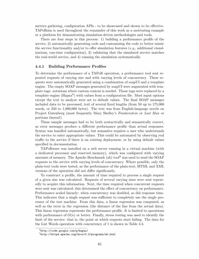
metrics gathering, configuration APIs - to be showcased and shown to be effective.TAPoRsim is used throughout the remainder of this work as a motivating exampleor a platform for demonstrating simulation-driven methodologies and tools.
There are four steps in this process: 1) building a performance profile of theservice, 2) automatically generating code and customizing the code to better mimicthe service functionality and/or to offer simulation features (e.g., additional visual-izations, run-time configuration), 3) validating that the simulated service matchesthe real-world service, and 4) running the simulation systematically.
4.4.1 Building Performance Profiles
To determine the performance of a TAPoR operation, a performance tool sent re-peated requests of varying size and with varying levels of concurrency. These re-quests were automatically generated using a combination of soapUI and a templateengine. The empty SOAP messages generated by soapUI were augmented with tem-plate tags: notations where custom content is needed. Those tags were replaced by atemplate engine (Hapax8) with values from a configuration file. Most input optionsexcept the text to analyze were set to default values. The final SOAP messagesincluded data to be processed, text of several fixed lengths (from 50 up to 175,000words, or 250 to 1,000,000 bytes). The text was from English-language novels onProject Gutenberg (most frequently Mary Shelley’s Frankenstein or Last Man orportions thereof).
These sample messages had to be both syntactically and semantically correct,as error messages produce a different performance profile than actual responses.Syntax was handled automatically, but semantics requires a user who understandsthe service to enter appropriate values. This could be automated by observing realtraffic to the service if there is an existing deployment, or by using default valuesspecified in documentation.
TAPoRware was installed on a web server running in a virtual machine (witha dedicated processor and reserved memory), which was configured with varyingamounts of memory. The Apache Benchmark (ab) tool9 was used to send the SOAPrequests to the service with varying levels of concurrency. Where possible, only theplain-text tools were tested, as the performance of the plain-text, HTML and XMLversions of the operation did not differ significantly.
To construct a profile, the amount of time required to process a single requestof a given size was calculated. Requests of several varying sizes were sent repeat-edly to acquire this information. Next, the time required when concurrent requestswere sent was calculated; this determined the effect of concurrency on performance.Performance scaled linearly: when concurrency was doubled, so did response time.This indicates that a single request was sufficient to completely use the single pro-cessor of the test machine. From this data, a linear regression was computed, aswell as the error in the regression (the distance of the line from the actual data).This linear regression represents the performance profile. It is limited to operationswith performance of O(n) or better. Finally, stress testing was used to identify thelimit of the service: that is, the point at which requests start failing. The data forthe List Words operation with concurrency of 1 is shown in Table 4.3.
8http://code.google.com/p/hapax/9http://httpd.apache.org/docs/2.0/programs/ab.html
65
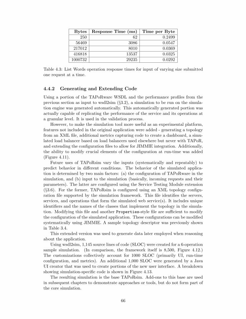
Bytes Response Time (ms) Time per Byte
250 62 0.2499
56469 3086 0.0547
217012 8010 0.0369
416818 13537 0.0325
1000732 29235 0.0292
Table 4.3: List Words operation response times for input of varying size submittedone request at a time.
4.4.2 Generating and Extending Code
Using a portion of the TAPoRware WSDL and the performance profiles from theprevious section as input to wsdl2sim (§3.2), a simulation to be run on the simula-tion engine was generated automatically. This automatically generated portion wasactually capable of replicating the performance of the service and its operations ata granular level. It is used in the validation process.
However, to make the simulation tool more useful as an experimental platform,features not included in the original application were added - generating a topologyfrom an XML file, additional metrics capturing code to create a dashboard, a simu-lated load balancer based on load balancers used elsewhere but never with TAPoR,and extending the configuration files to allow for JIMMIE integration. Additionally,the ability to modify crucial elements of the configuration at run-time was added(Figure 4.11).
Future uses of TAPoRsim vary the inputs (systematically and repeatably) topredict behavior in different conditions. The behavior of the simulated applica-tion is determined by two main factors: (a) the configuration of TAPoRware in thesimulation, and (b) input to the simulation (basically, incoming requests and theirparameters). The latter are configured using the Service Testing Module extension(§3.6). For the former, TAPoRsim is configured using an XML topology configu-ration file supported by the simulation framework. This file identifies the servers,services, and operations that form the simulated web service(s). It includes uniqueidentifiers and the names of the classes that implement the topology in the simula-tion. Modifying this file and another Properties-style file are sufficient to modifythe configuration of the simulated application. These configurations can be modifiedsystematically using JIMMIE. A sample topology descriptor was previously shownin Table 3.4.
This extended version was used to generate data later employed when reasoningabout the application.
Using wsdl2sim, 1,145 source lines of code (SLOC) were created for a 6-operationsample simulation. (In comparison, the framework itself is 8,500, Figure 4.12.)The customizations collectively account for 1000 SLOC (primarily UI, run-timeconfiguration, and metrics). An additional 1,000 SLOC were generated by a JavaUI creator that was used to create portions of the new user interface. A breakdownshowing simulation-specific code is shown in Figure 4.13.
The resulting simulation is the base TAPoRsim. Add-ons to this base are usedin subsequent chapters to demonstrate approaches or tools, but do not form part ofthe core simulation.
66
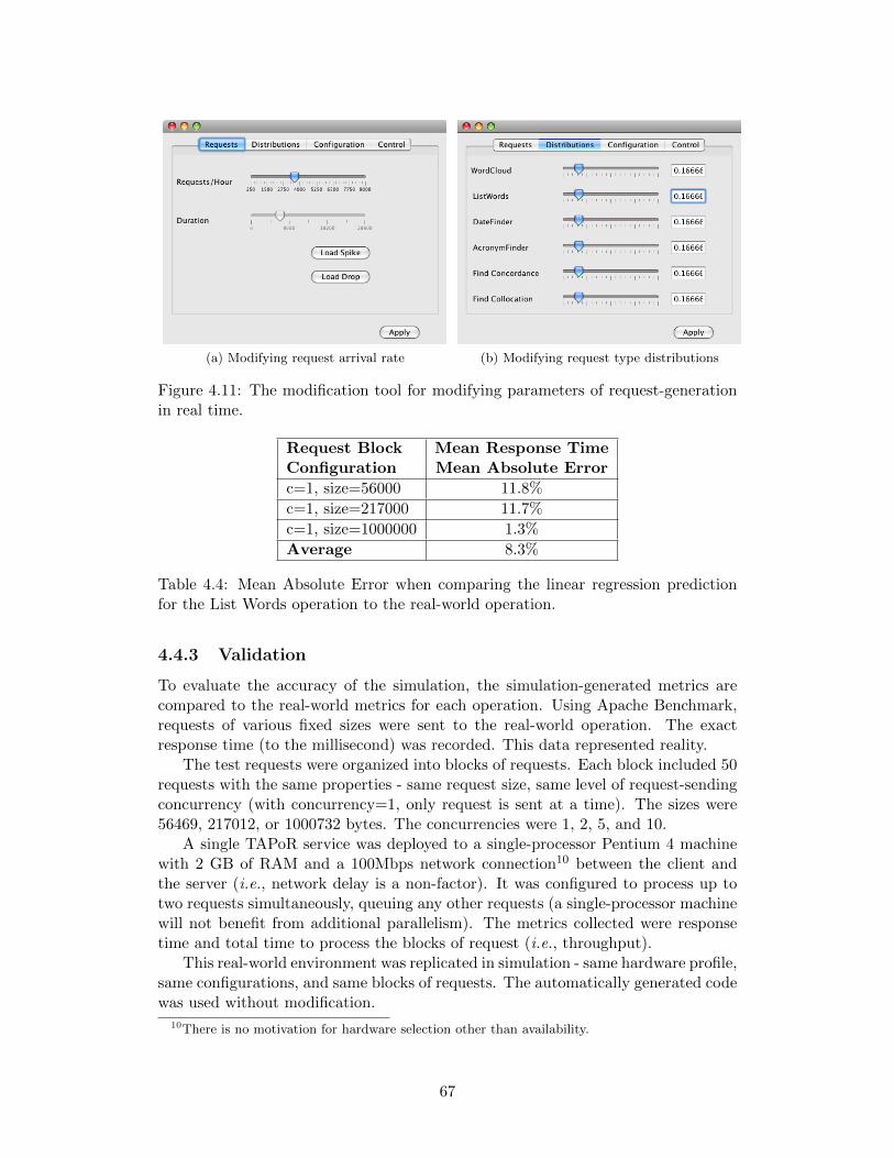
(a) Modifying request arrival rate (b) Modifying request type distributions
Figure 4.11: The modification tool for modifying parameters of request-generationin real time.
Request Block Mean Response TimeConfiguration Mean Absolute Error
c=1, size=56000 11.8%
c=1, size=217000 11.7%
c=1, size=1000000 1.3%
Average 8.3%
Table 4.4: Mean Absolute Error when comparing the linear regression predictionfor the List Words operation to the real-world operation.
4.4.3 Validation
To evaluate the accuracy of the simulation, the simulation-generated metrics arecompared to the real-world metrics for each operation. Using Apache Benchmark,requests of various fixed sizes were sent to the real-world operation. The exactresponse time (to the millisecond) was recorded. This data represented reality.
The test requests were organized into blocks of requests. Each block included 50requests with the same properties - same request size, same level of request-sendingconcurrency (with concurrency=1, only request is sent at a time). The sizes were56469, 217012, or 1000732 bytes. The concurrencies were 1, 2, 5, and 10.
A single TAPoR service was deployed to a single-processor Pentium 4 machinewith 2 GB of RAM and a 100Mbps network connection10 between the client andthe server (i.e., network delay is a non-factor). It was configured to process up totwo requests simultaneously, queuing any other requests (a single-processor machinewill not benefit from additional parallelism). The metrics collected were responsetime and total time to process the blocks of request (i.e., throughput).
This real-world environment was replicated in simulation - same hardware profile,same configurations, and same blocks of requests. The automatically generated codewas used without modification.
10There is no motivation for hardware selection other than availability.
67
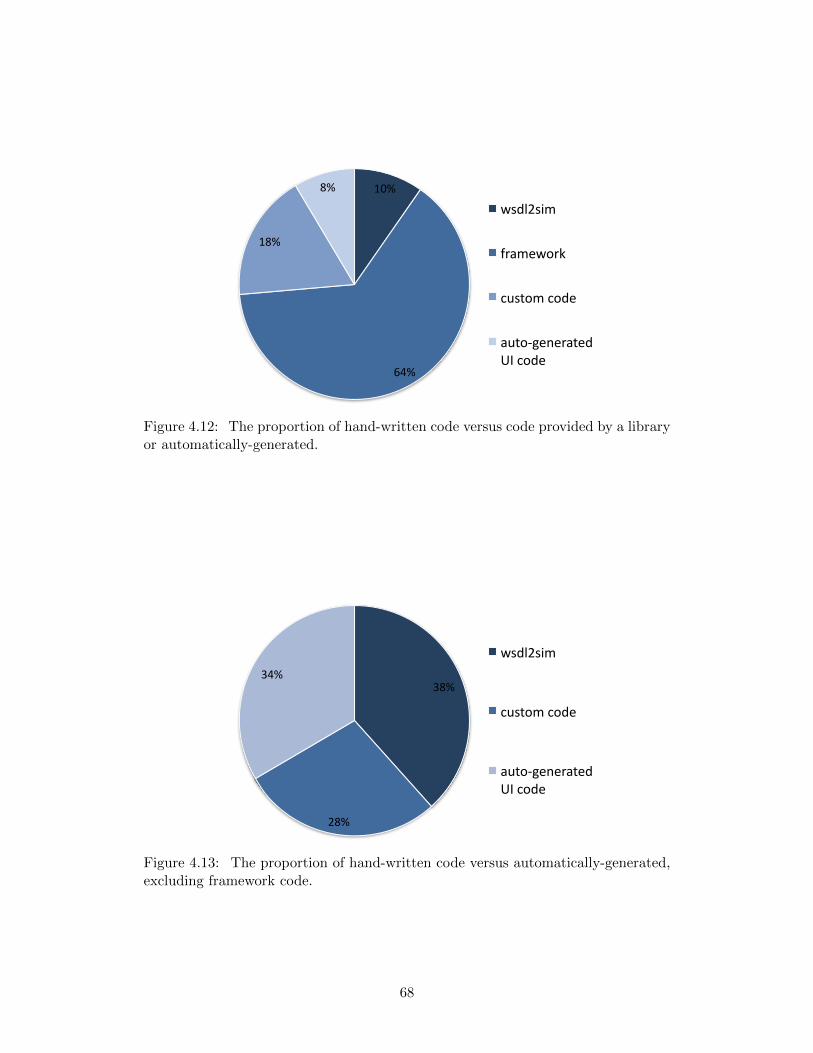
10%
64%
18%
8%
wsdl2sim
framework
custom code
auto‐generated UI code
Figure 4.12: The proportion of hand-written code versus code provided by a libraryor automatically-generated.
38%
28%
34%
wsdl2sim
custom code
auto-‐generated UI code
Figure 4.13: The proportion of hand-written code versus automatically-generated,excluding framework code.
68
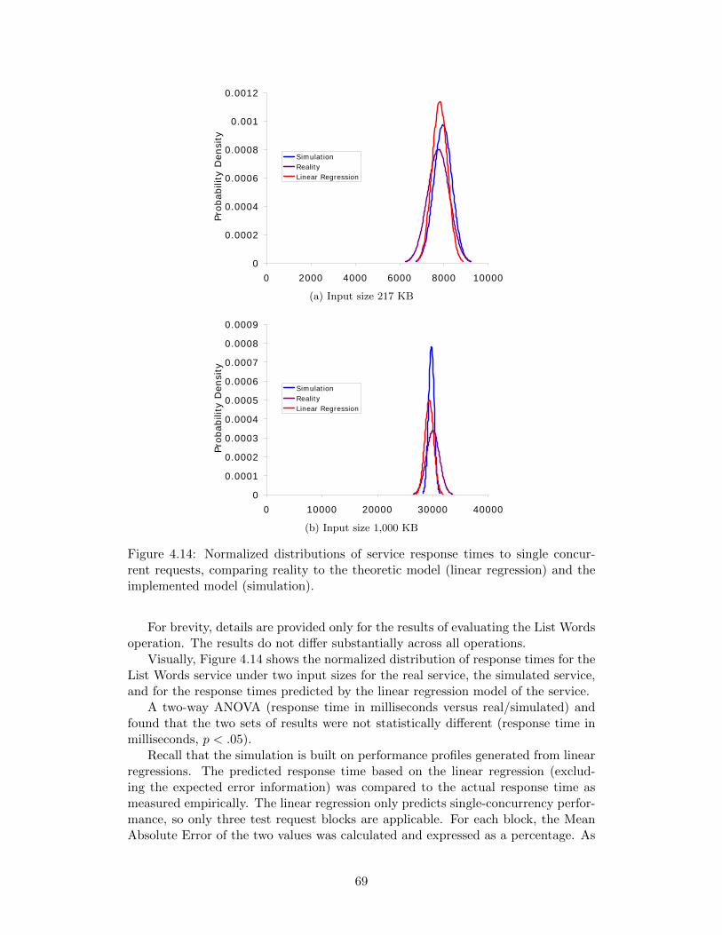
0
0.0002
0.0004
0.0006
0.0008
0.001
0.0012
0 2000 4000 6000 8000 10000
Probab
ility
Den
sity
SimulationRealityLinear Regression
(a) Input size 217 KB
0
0.0001
0.0002
0.0003
0.0004
0.0005
0.0006
0.0007
0.0008
0.0009
0 10000 20000 30000 40000
Probab
ility
Den
sity
SimulationRealityLinear Regression
(b) Input size 1,000 KB
Figure 4.14: Normalized distributions of service response times to single concur-rent requests, comparing reality to the theoretic model (linear regression) and theimplemented model (simulation).
For brevity, details are provided only for the results of evaluating the List Wordsoperation. The results do not differ substantially across all operations.
Visually, Figure 4.14 shows the normalized distribution of response times for theList Words service under two input sizes for the real service, the simulated service,and for the response times predicted by the linear regression model of the service.
A two-way ANOVA (response time in milliseconds versus real/simulated) andfound that the two sets of results were not statistically different (response time inmilliseconds, p < .05).
Recall that the simulation is built on performance profiles generated from linearregressions. The predicted response time based on the linear regression (exclud-ing the expected error information) was compared to the actual response time asmeasured empirically. The linear regression only predicts single-concurrency perfor-mance, so only three test request blocks are applicable. For each block, the MeanAbsolute Error of the two values was calculated and expressed as a percentage. As
69
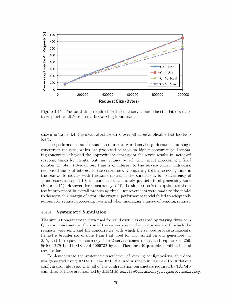
0
200
400
600
800
1000
1200
1400
1600
0 200000 400000 600000 800000 1000000
Proc
essi
ng T
ime
for A
ll R
eque
sts
(s)
Request Size (Bytes)
C=1, Real
C=1, Sim
C=10, Real
C=10, Sim
Figure 4.15: The total time required for the real service and the simulated serviceto respond to all 50 requests for varying input sizes.
shown in Table 4.4, the mean absolute error over all three applicable test blocks is8.3%.
The performance model was based on real-world service performance for singleconcurrent requests, which are projected to scale to higher concurrency. Increas-ing concurrency beyond the approximate capacity of the server results in increasedresponse times for clients, but may reduce overall time spent processing a fixednumber of jobs. (Overall test time is of interest to the service owner; individualresponse time is of interest to the consumer). Comparing total processing time inthe real-world service with the same metric in the simulation, for concurrency of1 and concurrency of 10, the simulation accurately predicts total processing time(Figure 4.15). However, for concurrency of 10, the simulation is too optimistic aboutthe improvement in overall processing time. Improvements were made to the modelto decrease this margin of error: the original performance model failed to adequatelyaccount for request processing overhead when managing a queue of pending request.
4.4.4 Systematic Simulation
The simulation-generated data used for validation was created by varying three con-figuration parameters: the size of the requests sent, the concurrency with which therequests were sent, and the concurrency with which the service processes requests.In fact a broader set of data than that used for the validation was generated: 1,2, 5, and 10 request concurrency; 1 or 2 service concurrency; and request size 250,56469, 217012, 416818, and 1000732 bytes. There are 40 possible combinations ofthese values.
To demonstrate the systematic simulation of varying configurations, this datawas generated using JIMMIE. The JIML file used is shown in Figure 4.16. A defaultconfiguration file is set with all of the configuration parameters required by TAPoR-sim; three of these are modified by JIMMIE: serviceConcurrency, requestConcurrency,
70
and size (of requests generated). The default value for each variable is set in thedefault configuration file (to 2, 10, and 250, respectively). JIMMIE only modifiesthe attributes when the default must be modified. So for instance, one commandchanges serviceConcurrency to 1 instead of 2 for half of the simulations (experi-ments 1 through 20); for the remainder, the default value is used. JIMMIE system-atically creates all combinations of the possible values, leaving untouched defaultparameters. All requests were sent to the List Words operation.
The simulation was run on a Pentium 4 machine with 1.75 GB of RAM, andsimulated the TAPoRware service running on a Pentium 4 machine with 2GB ofRAM. The results produced by JIMMIE are shown in Table 4.5. Sending more thanone request at a time to a single-processor service increases the overall response timeas requests contend for resources or spend time waiting in a queue; the total timetaken to process the requests doesn’t change.
Using this systematic simulation as well as stand-alone simulations, over 1,000,000,000individual metrics have been collected during the experiments described in this dis-sertation.
4.4.5 Known Issues and Threats to Validity
The automatic generation (wsdl2sim) is limited to operations with performance ofO(n) or better. This could be extended by replacing the linear regression and linearmodels used; regression analysis and curve-fitting is generally applicable to higher-order polynomials (though limited by the abilities of curve fitting on higher-orderpolynomials), exponential growth, etc..
The validation was performed on two key metrics (response time and total time)in a straightforward application configuration. The assertion is that the validityof (some) other metrics and the validity of metrics in more complex scenarios fol-lows from this validation. Though these two key metrics are used predominantlythroughout the remainder of this work, other metrics are occasionally employed andare not as thoroughly validated. In most cases, a real-world implementation is testedto further validate the simulation-based results.
Only the CPU use is tracked and used to govern response time; if a machinehas substantially more CPU available than memory, memory may prove to be thebottleneck. Such scenarios are not anticipated by the simulation.
4.5 Summary
This chapter described the process of using SASF (Chapter 3) to simulate TivoliProvisioning Manager and the back-end service for the Text Analysis Portal forResearch. The first demonstrates use of basic library functionality, the simulationengine, and the metrics engine. The second adds the use of additional libraries,automated simulation generation, systematic simulation using JIMMIE, and theService Testing Module. One remaining SASF extension, the emulation extension,will be used in later chapters and is not used in the base versions of TPMsim orTAPoRsim.
The use of the framework reduced development time and effort that would havebeen required otherwise. In the case of TPMsim, the framework is estimated tohave offered a 45% reduction in development effort. In the case of TAPoRsim, its
71

behavior was replicated without manually authoring a single line of code. A setof extensions was added, and still only 28% of the TAPoRsim-specific code washand-coded.
TAPoRsim will be used to test, demonstrate, and validate the methodologiesand tools in the following chapters.
72
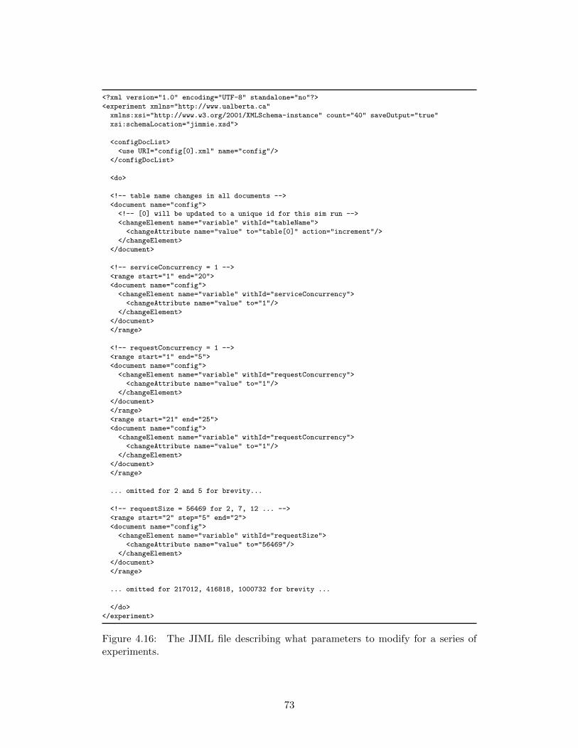
<?xml version="1.0" encoding="UTF-8" standalone="no"?>
<experiment xmlns="http://www.ualberta.ca"
xmlns:xsi="http://www.w3.org/2001/XMLSchema-instance" count="40" saveOutput="true"
xsi:schemaLocation="jimmie.xsd">
<configDocList>
<use URI="config[0].xml" name="config"/>
</configDocList>
<do>
<!-- table name changes in all documents -->
<document name="config">
<!-- [0] will be updated to a unique id for this sim run -->
<changeElement name="variable" withId="tableName">
<changeAttribute name="value" to="table[0]" action="increment"/>
</changeElement>
</document>
<!-- serviceConcurrency = 1 -->
<range start="1" end="20">
<document name="config">
<changeElement name="variable" withId="serviceConcurrency">
<changeAttribute name="value" to="1"/>
</changeElement>
</document>
</range>
<!-- requestConcurrency = 1 -->
<range start="1" end="5">
<document name="config">
<changeElement name="variable" withId="requestConcurrency">
<changeAttribute name="value" to="1"/>
</changeElement>
</document>
</range>
<range start="21" end="25">
<document name="config">
<changeElement name="variable" withId="requestConcurrency">
<changeAttribute name="value" to="1"/>
</changeElement>
</document>
</range>
... omitted for 2 and 5 for brevity...
<!-- requestSize = 56469 for 2, 7, 12 ... -->
<range start="2" step="5" end="2">
<document name="config">
<changeElement name="variable" withId="requestSize">
<changeAttribute name="value" to="56469"/>
</changeElement>
</document>
</range>
... omitted for 217012, 416818, 1000732 for brevity ...
</do>
</experiment>
Figure 4.16: The JIML file describing what parameters to modify for a series ofexperiments.
73
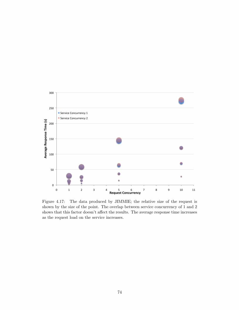
0
50
100
150
200
250
300
0 1 2 3 4 5 6 7 8 9 10 11
Average Respo
nse Time (s)
Request Concurrency
Service Concurrency 1
Service Concurrency 2
Figure 4.17: The data produced by JIMMIE; the relative size of the request isshown by the size of the point. The overlap between service concurrency of 1 and 2shows that this factor doesn’t affect the results. The average response time increasesas the request load on the service increases.
74
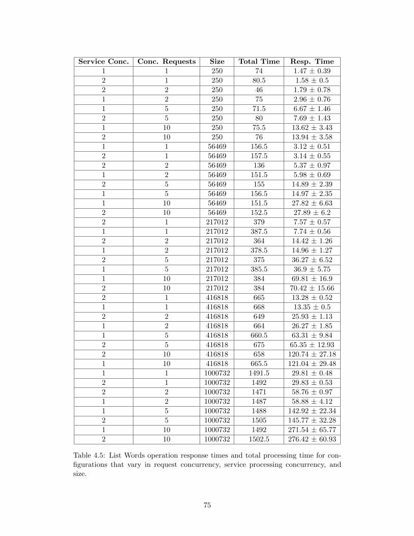
Service Conc. Conc. Requests Size Total Time Resp. Time
1 1 250 74 1.47 ± 0.39
2 1 250 80.5 1.58 ± 0.5
2 2 250 46 1.79 ± 0.78
1 2 250 75 2.96 ± 0.76
1 5 250 71.5 6.67 ± 1.46
2 5 250 80 7.69 ± 1.43
1 10 250 75.5 13.62 ± 3.43
2 10 250 76 13.94 ± 3.58
1 1 56469 156.5 3.12 ± 0.51
2 1 56469 157.5 3.14 ± 0.55
2 2 56469 136 5.37 ± 0.97
1 2 56469 151.5 5.98 ± 0.69
2 5 56469 155 14.89 ± 2.39
1 5 56469 156.5 14.97 ± 2.35
1 10 56469 151.5 27.82 ± 6.63
2 10 56469 152.5 27.89 ± 6.2
2 1 217012 379 7.57 ± 0.57
1 1 217012 387.5 7.74 ± 0.56
2 2 217012 364 14.42 ± 1.26
1 2 217012 378.5 14.96 ± 1.27
2 5 217012 375 36.27 ± 6.52
1 5 217012 385.5 36.9 ± 5.75
1 10 217012 384 69.81 ± 16.9
2 10 217012 384 70.42 ± 15.66
2 1 416818 665 13.28 ± 0.52
1 1 416818 668 13.35 ± 0.5
2 2 416818 649 25.93 ± 1.13
1 2 416818 664 26.27 ± 1.85
1 5 416818 660.5 63.31 ± 9.84
2 5 416818 675 65.35 ± 12.93
2 10 416818 658 120.74 ± 27.18
1 10 416818 665.5 121.04 ± 29.48
1 1 1000732 1491.5 29.81 ± 0.48
2 1 1000732 1492 29.83 ± 0.53
2 2 1000732 1471 58.76 ± 0.97
1 2 1000732 1487 58.88 ± 4.12
1 5 1000732 1488 142.92 ± 22.34
2 5 1000732 1505 145.77 ± 32.28
1 10 1000732 1492 271.54 ± 65.77
2 10 1000732 1502.5 276.42 ± 60.93
Table 4.5: List Words operation response times and total processing time for con-figurations that vary in request concurrency, service processing concurrency, andsize.
75

Chapter 5
Informing the SLA Lifecycleusing Simulation
Chapter Contents
5.1 Negotiation . . . . . . . . . . . . . . 77
5.1.1 Simulation-supported SLA Ne-gotiation . . . . . . . . . . . . . 80
5.2 Configuration and Deployment . . . 83
5.2.1 Simulation-supported Configu-ration and Deployment . . . . . 83
5.3 Execution and Assessment . . . . . . 87
5.3.1 SASF-supported Executionand Assessment . . . . . . . . . 88
5.4 Summary . . . . . . . . . . . . . . . 89
An SLA can be viewed as a three-way relationship among the producer,the consumer1, and the service. Thetypical lifecycle of an SLA involvescreation (negotiation), implementationand assessment, and eventually termi-nation (Figure 5.1). This is the pre-vailing view on SLA lifecycles (e.g.,[23, 24]). Others recognize the need forthe SLA to evolve and be re-negotiatedover its lifetime (e.g., [6, 25]). The lat-ter view is adopted here, and extended:the SLA should evolve as business needs change, based on periodic review, and asthe service implementation itself evolves (for example, to add new features).
This modified view of the SLA lifecycle is shown in Figure 5.2 by changing thelinear process into a more realistic cycle. An initial SLA is negotiated to documentthe desired qualities of the service delivery. The service is configured and deployedto meet the SLA. Service interactions are monitored and evaluated to ensure thatthe terms of the SLA are met. The important part is the SLA is not static - itis periodically re-negotiated, or at least re-examined, to ensure it is still practical.Good points for re-examination are when the software is updated and when businessneeds change. The result of the evaluation or the re-negotiation may be to terminatethe SLA.
Each phase of the lifecycle and a simulation-driven method addressing that phaseis described in the following sections. §5.1 describes the challenges that face a con-sumer negotiating with a service provider who has more information and under-standing about the service. It presents simulation-driven approaches to assisting inmaking choices and trade-offs explicit and well understood to strike a balance thatprovides actual and lasting quality to the consumer. §5.2 describes the process oftranslating an SLA into a configuration, and introduces a simulation-driven question
1The consumer is not an individual; it is any entity that consumes a service. A service is nottechnically “consumed”, but the term “user” is even more overloaded.
76
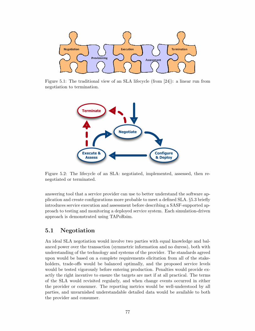
customer and a service provider. The objective of Section 3 is to initiate discussion at the workshop on novel dynamic pricing strategies and Section 4 provides a high level architecture for SLA management. Future research is presented in Section 5 followed by a conclusion.
2. SLA LIFECYCLE EServices are services that provide their functionality electronically and the interaction between the customer and provider is through a communication network. There is no constraint as to what these services provide – they could provide simple weather forecasts and stock quotes or resource intensive simulations of complex systems.
Before a customer gets access to a provider’s service, they need to establish a contract that regulates that access. SLAs are one expression of such a contract. A typical scenario between a customer and a service provider is that they first negotiate an SLA that includes price, service type and quality of service attributes. We envisage that SLAs provide the foundations to the successful establishment of a sustainable eServices marketplace. Service usage will be governed by SLAs under a well-established legal framework.
A key parameter in determining a base price for a service is the cost for the provider to provide the service. The cost includes the purchase and maintenance of hardware and software, network access, and risks. Non-functional properties in an agreement are another important parameter in negotiating a price for the service – an SLA with tight time constraints will be of greater risk to the provider and thus will incur a greater price.
The complete lifecycle of an SLA is described by the TeleManagement Forum [3] and is split into six distinct phases as listed below:
• Development of Service and SLA Templates
• Discovery and Negotiation of an SLA
• Service Provisioning and deployment
• Execution of the Service
• Assessment and corrective actions during execution (parallel phase to execution of the service)
• Termination and Decommission of the Service
There is still ongoing discussion as to whether the creation of a service and SLA template should be part of the lifecycle or whether is it a predecessor of the lifecycle. We see it as a predecessor and not as part of the lifecycle as depicted in Figure 1.
Figure 1: SLA life cycle
The creation of SLA templates for an eService identifies and defines the non-functional quality of service attributes and the
price, which impacts all the later stages of the SLA lifecycle including negotiation, monitoring and service provisioning.
Introducing dynamic pricing into SLA negotiation affects the service and SLA template development stage. In addition to developing the service and its associated SLA templates, additional effort needs to be invested in developing and realizing pricing policies that match the service function and quality attributes.
After the negotiation of an SLA the service provider has to configure his system accordingly to provide the service to the customer. He is now prepared for the execution of the service whose quality will be assessed (e.g. for accounting and billing purposes) until the SLA is terminated. Within this paper we concentrate on the first phase of the SLA lifecycle – the negotiation.
Negotiation between customer and provider is achieved through a negotiation protocol. Our position is that the eServices community should adopt the protocol that has been abstractly defined by contract law [6] and it is surprisingly simple and well-defined. Essentially, the customer uses the SLA template to make the service provider an offer, the provider acknowledges the receipt of the offer and then either accepts or rejects the offer. In the former case, an SLA has been established while in the latter the provider may provide reasons (similar to a quote) as to why the offer was rejected to aid the customer make a new offer that is more likely to be accepted.
The reason why service providers do not make offers is to prevent denial-of-service attacks as explained in Parkin et al. [7]. In contract law, quotes are not legally binding meaning that a service provider has no legal obligations to accept an offer based on a past quote – however, rejecting offers based on quotes may damage a provider’s reputation and reduce its profitability.
With dynamic pricing, the price may change while the customer and service provider are negotiating an SLA. Essentially, the service provider needs to calculate a price in real time based on the current state of the marketplace (supply and demand), historical data to predict future supply and demand, the provider’s business objectives and risks. The price can in practice, for the same SLA, change every minute in a highly dynamic marketplace similar to stock markets.
It is important to note that once a SLA has been established the price is fixed between the service provider and customer.
3. DYNAMIC PRICING Dynamic pricing refers to the continuous changing of the price for goods and services. The fluctuation results from the constant change in the supply and demand of the marketplace – in general, prices go up when supply is low or demand is high while prices go down when supply is high or demand is low. Dynamic pricing affects how customers and providers negotiate SLAs as the price can change significantly during negotiation. However, it is important to note that once an SLA has been agreed to – that is, a contract has been established – then the price is fixed for the remainder of the lifetime of the SLA. The establishment of an SLA and the setting of a certain price affect that particular provider-consumer interaction only. The price for the same service provided to another customer might be different.
Figure 5.1: The traditional view of an SLA lifecycle (from [24]): a linear run fromnegotiation to termination.
Negotiate
Configure & Deploy
Execute & Assess
Terminate
Figure 5.2: The lifecycle of an SLA: negotiated, implemented, assessed, then re-negotiated or terminated.
answering tool that a service provider can use to better understand the software ap-plication and create configurations more probable to meet a defined SLA. §5.3 brieflyintroduces service execution and assessment before describing a SASF-supported ap-proach to testing and monitoring a deployed service system. Each simulation-drivenapproach is demonstrated using TAPoRsim.
5.1 Negotiation
An ideal SLA negotiation would involve two parties with equal knowledge and bal-anced power over the transaction (symmetric information and no duress), both withunderstanding of the technology and systems of the provider. The standards agreedupon would be based on a complete requirements elicitation from all of the stake-holders, trade-offs would be balanced optimally, and the proposed service levelswould be tested vigorously before entering production. Penalties would provide ex-actly the right incentive to ensure the targets are met if at all practical. The termsof the SLA would revisited regularly, and when change events occurred in eitherthe provider or consumer. The reporting metrics would be well-understood by allparties, and unvarnished understandable detailed data would be available to boththe provider and consumer.
77
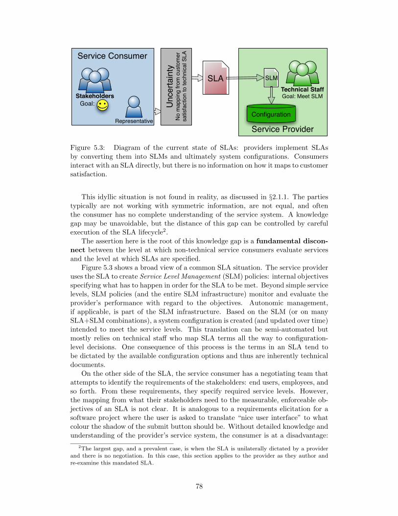
Service Consumer
Service Provider
SLA
Configuration
Technical StaffGoal: Meet SLMStakeholders
Goal:
SLM
Unc
erta
inty
No
map
ping
from
cus
tom
ersa
tisfa
ctio
n to
tech
nica
l SLA
Representative
Figure 5.3: Diagram of the current state of SLAs: providers implement SLAsby converting them into SLMs and ultimately system configurations. Consumersinteract with an SLA directly, but there is no information on how it maps to customersatisfaction.
This idyllic situation is not found in reality, as discussed in §2.1.1. The partiestypically are not working with symmetric information, are not equal, and oftenthe consumer has no complete understanding of the service system. A knowledgegap may be unavoidable, but the distance of this gap can be controlled by carefulexecution of the SLA lifecycle2.
The assertion here is the root of this knowledge gap is a fundamental discon-nect between the level at which non-technical service consumers evaluate servicesand the level at which SLAs are specified.
Figure 5.3 shows a broad view of a common SLA situation. The service provideruses the SLA to create Service Level Management (SLM) policies: internal objectivesspecifying what has to happen in order for the SLA to be met. Beyond simple servicelevels, SLM policies (and the entire SLM infrastructure) monitor and evaluate theprovider’s performance with regard to the objectives. Autonomic management,if applicable, is part of the SLM infrastructure. Based on the SLM (or on manySLA+SLM combinations), a system configuration is created (and updated over time)intended to meet the service levels. This translation can be semi-automated butmostly relies on technical staff who map SLA terms all the way to configuration-level decisions. One consequence of this process is the terms in an SLA tend tobe dictated by the available configuration options and thus are inherently technicaldocuments.
On the other side of the SLA, the service consumer has a negotiating team thatattempts to identify the requirements of the stakeholders: end users, employees, andso forth. From these requirements, they specify required service levels. However,the mapping from what their stakeholders need to the measurable, enforceable ob-jectives of an SLA is not clear. It is analogous to a requirements elicitation for asoftware project where the user is asked to translate “nice user interface” to whatcolour the shadow of the submit button should be. Without detailed knowledge andunderstanding of the provider’s service system, the consumer is at a disadvantage:
2The largest gap, and a prevalent case, is when the SLA is unilaterally dictated by a providerand there is no negotiation. In this case, this section applies to the provider as they author andre-examine this mandated SLA.
78
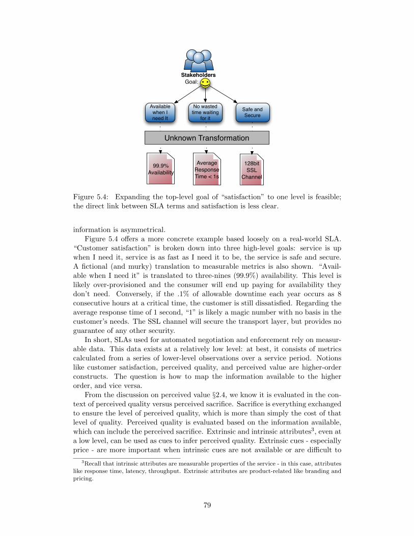
Stakeholders Goal:
99.9%Availability
Available when I need It
No wasted time waiting
for it
AverageResponseTime < 1s
Safe and Secure
128bitSSL
Channel
Unknown Transformation
Figure 5.4: Expanding the top-level goal of “satisfaction” to one level is feasible;the direct link between SLA terms and satisfaction is less clear.
information is asymmetrical.Figure 5.4 offers a more concrete example based loosely on a real-world SLA.
“Customer satisfaction” is broken down into three high-level goals: service is upwhen I need it, service is as fast as I need it to be, the service is safe and secure.A fictional (and murky) translation to measurable metrics is also shown. “Avail-able when I need it” is translated to three-nines (99.9%) availability. This level islikely over-provisioned and the consumer will end up paying for availability theydon’t need. Conversely, if the .1% of allowable downtime each year occurs as 8consecutive hours at a critical time, the customer is still dissatisfied. Regarding theaverage response time of 1 second, “1” is likely a magic number with no basis in thecustomer’s needs. The SSL channel will secure the transport layer, but provides noguarantee of any other security.
In short, SLAs used for automated negotiation and enforcement rely on measur-able data. This data exists at a relatively low level: at best, it consists of metricscalculated from a series of lower-level observations over a service period. Notionslike customer satisfaction, perceived quality, and perceived value are higher-orderconstructs. The question is how to map the information available to the higherorder, and vice versa.
From the discussion on perceived value §2.4, we know it is evaluated in the con-text of perceived quality versus perceived sacrifice. Sacrifice is everything exchangedto ensure the level of perceived quality, which is more than simply the cost of thatlevel of quality. Perceived quality is evaluated based on the information available,which can include the perceived sacrifice. Extrinsic and intrinsic attributes3, even ata low level, can be used as cues to infer perceived quality. Extrinsic cues - especiallyprice - are more important when intrinsic cues are not available or are difficult to
3Recall that intrinsic attributes are measurable properties of the service - in this case, attributeslike response time, latency, throughput. Extrinsic attributes are product-related like branding andpricing.
79

evaluate; they are used as “value signals”. Intrinsic cues are more important whenthey are search attributes4 and tend to be accurate predictors of value. Intrinsicattributes that are more abstract are more broadly application. §5.1.1 describessimulation support for negotiation that is an early attempt at addressing these is-sues.
Service providers are motivated to provide value to service consumers at eval-uation time: in an ongoing service-relationship, customer satisfaction is necessaryfor the continuation of the relationship5. In service encounters, a trusted providerhas the opportunity to influence how the consumer perceives quality (Nilsson, [53]).Though perceived value and perceived quality can be influenced at negotiation timeby exploiting the understanding of value as described above, this influence will bediminished at evaluation time. As discussed in §2.4, assessment of perceived value issituational and can change between purchase time and deployment, as more infor-mation becomes available. An SLA negotiated with artificially skewed perceptionsof quality and cost will likely prove to be unsatisfactory once implemented, and thetrust relationship may be impacted. The service provider is incentivized to assistthe consumer in reaching an SLA that satisfies them.
5.1.1 Simulation-supported SLA Negotiation
Creating an SLA involves reconciling a set of goals, which might be well-specified oronly intuitively understood, and might be complementary or might conflict. Thistrade-off analysis methodology supports decisions involving the balancing of con-flicting goals, whereby one might relax goals in one area in order to achieve othergoals, perceived as more important. Without loss of generality, this discussion isfocused on cost and performance metrics, as they are common and more readilyquantifiable. One of the shortcomings of SLAs identified by Blomberg [6] was thatthe parties involved in creating SLAs lacked the information and intuition needed tomake appropriate decisions about quality of service levels; this approach attemptsto provide both information and intuition when planning.
Experts can ask and answer specific questions about a software service system.When the goal is a general exploration of the trade-offs, a large number of possibleconfigurations can be simulated to generate a knowledge base that powers a decisionsupport tool. Using this knowledge base, various conflicting or correlated metrics arevisualized to understand the impact that one goal will have on another. The systemmanager can select potentially viable configurations using a visual tool. Based ontheir selections, a “fitness score” is calculated for each configuration.
Visual Selection Tool. The configuration exploration simulations are visu-alized as a series of weighted scatter plots in a two-dimensional space, where thetwo axes correspond to two metrics, offering a head-to-head comparison. For ex-ample, Figure 5.5 shows a sample plot of correlated values, the average responsetime (x) versus the total time required to complete the processing. The configu-rations are clustered based on their values for the two metrics. Each point on theplot corresponds to a cluster, and is sized based on the number of configurationsthat belong in this cluster. The user is shown a series of these plots and is asked
4Recall that search attributes can be assessed before experience with the product or service;experience attributes are assessed only during consumption.
5Excluding, of course, monopolies and oligopolies
80
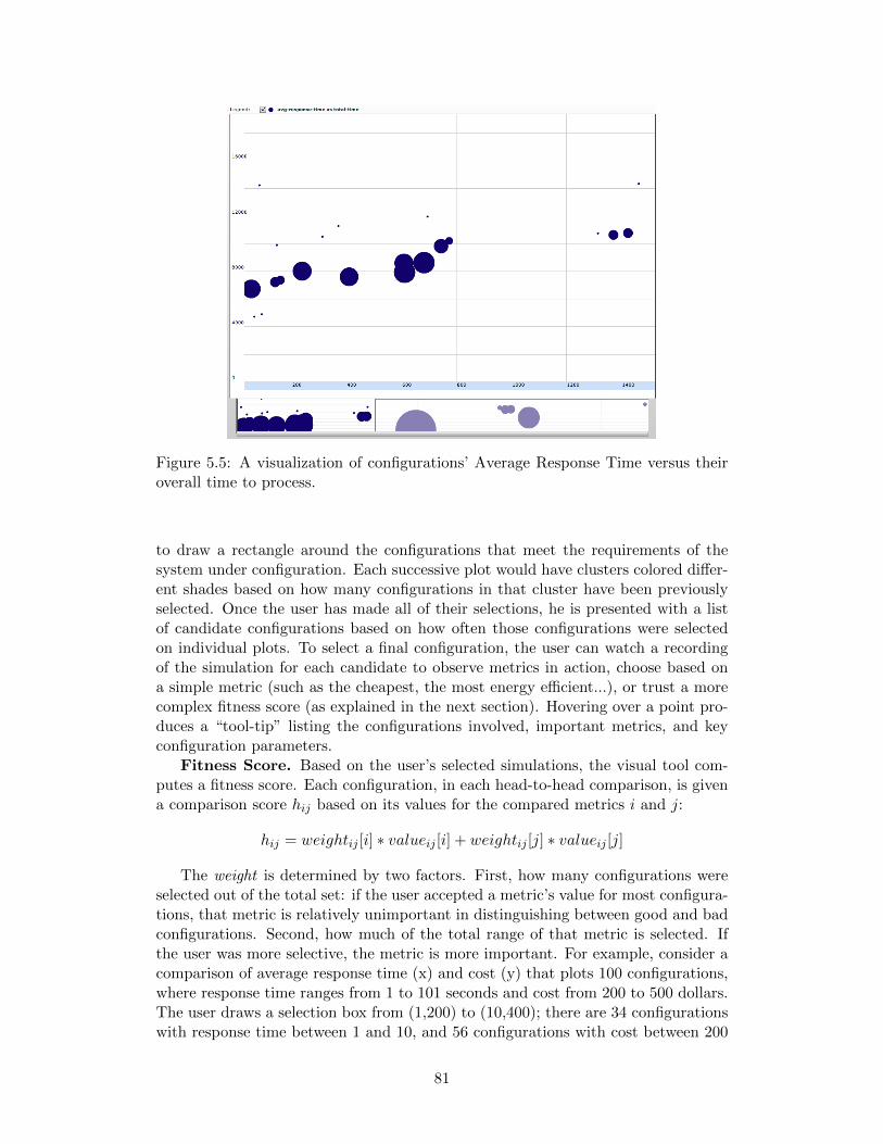
Figure 5.5: A visualization of configurations’ Average Response Time versus theiroverall time to process.
to draw a rectangle around the configurations that meet the requirements of thesystem under configuration. Each successive plot would have clusters colored differ-ent shades based on how many configurations in that cluster have been previouslyselected. Once the user has made all of their selections, he is presented with a listof candidate configurations based on how often those configurations were selectedon individual plots. To select a final configuration, the user can watch a recordingof the simulation for each candidate to observe metrics in action, choose based ona simple metric (such as the cheapest, the most energy efficient...), or trust a morecomplex fitness score (as explained in the next section). Hovering over a point pro-duces a “tool-tip” listing the configurations involved, important metrics, and keyconfiguration parameters.
Fitness Score. Based on the user’s selected simulations, the visual tool com-putes a fitness score. Each configuration, in each head-to-head comparison, is givena comparison score hij based on its values for the compared metrics i and j:
hij = weightij [i] ∗ valueij [i] + weightij [j] ∗ valueij [j]
The weight is determined by two factors. First, how many configurations wereselected out of the total set: if the user accepted a metric’s value for most configura-tions, that metric is relatively unimportant in distinguishing between good and badconfigurations. Second, how much of the total range of that metric is selected. Ifthe user was more selective, the metric is more important. For example, consider acomparison of average response time (x) and cost (y) that plots 100 configurations,where response time ranges from 1 to 101 seconds and cost from 200 to 500 dollars.The user draws a selection box from (1,200) to (10,400); there are 34 configurationswith response time between 1 and 10, and 56 configurations with cost between 200
81
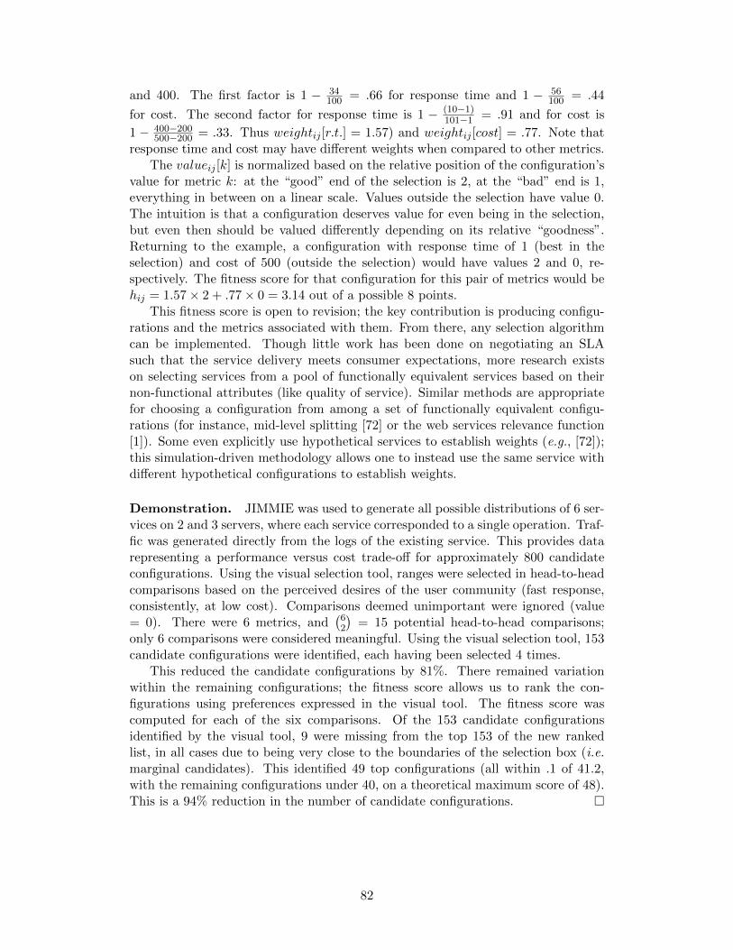
and 400. The first factor is 1 − 34100 = .66 for response time and 1 − 56
100 = .44
for cost. The second factor for response time is 1 − (10−1)101−1 = .91 and for cost is
1 − 400−200500−200 = .33. Thus weightij [r.t.] = 1.57) and weightij [cost] = .77. Note that
response time and cost may have different weights when compared to other metrics.The valueij [k] is normalized based on the relative position of the configuration’s
value for metric k: at the “good” end of the selection is 2, at the “bad” end is 1,everything in between on a linear scale. Values outside the selection have value 0.The intuition is that a configuration deserves value for even being in the selection,but even then should be valued differently depending on its relative “goodness”.Returning to the example, a configuration with response time of 1 (best in theselection) and cost of 500 (outside the selection) would have values 2 and 0, re-spectively. The fitness score for that configuration for this pair of metrics would behij = 1.57× 2 + .77× 0 = 3.14 out of a possible 8 points.
This fitness score is open to revision; the key contribution is producing configu-rations and the metrics associated with them. From there, any selection algorithmcan be implemented. Though little work has been done on negotiating an SLAsuch that the service delivery meets consumer expectations, more research existson selecting services from a pool of functionally equivalent services based on theirnon-functional attributes (like quality of service). Similar methods are appropriatefor choosing a configuration from among a set of functionally equivalent configu-rations (for instance, mid-level splitting [72] or the web services relevance function[1]). Some even explicitly use hypothetical services to establish weights (e.g., [72]);this simulation-driven methodology allows one to instead use the same service withdifferent hypothetical configurations to establish weights.
Demonstration. JIMMIE was used to generate all possible distributions of 6 ser-vices on 2 and 3 servers, where each service corresponded to a single operation. Traf-fic was generated directly from the logs of the existing service. This provides datarepresenting a performance versus cost trade-off for approximately 800 candidateconfigurations. Using the visual selection tool, ranges were selected in head-to-headcomparisons based on the perceived desires of the user community (fast response,consistently, at low cost). Comparisons deemed unimportant were ignored (value= 0). There were 6 metrics, and
(62
)= 15 potential head-to-head comparisons;
only 6 comparisons were considered meaningful. Using the visual selection tool, 153candidate configurations were identified, each having been selected 4 times.
This reduced the candidate configurations by 81%. There remained variationwithin the remaining configurations; the fitness score allows us to rank the con-figurations using preferences expressed in the visual tool. The fitness score wascomputed for each of the six comparisons. Of the 153 candidate configurationsidentified by the visual tool, 9 were missing from the top 153 of the new rankedlist, in all cases due to being very close to the boundaries of the selection box (i.e.marginal candidates). This identified 49 top configurations (all within .1 of 41.2,with the remaining configurations under 40, on a theoretical maximum score of 48).This is a 94% reduction in the number of candidate configurations. �
82
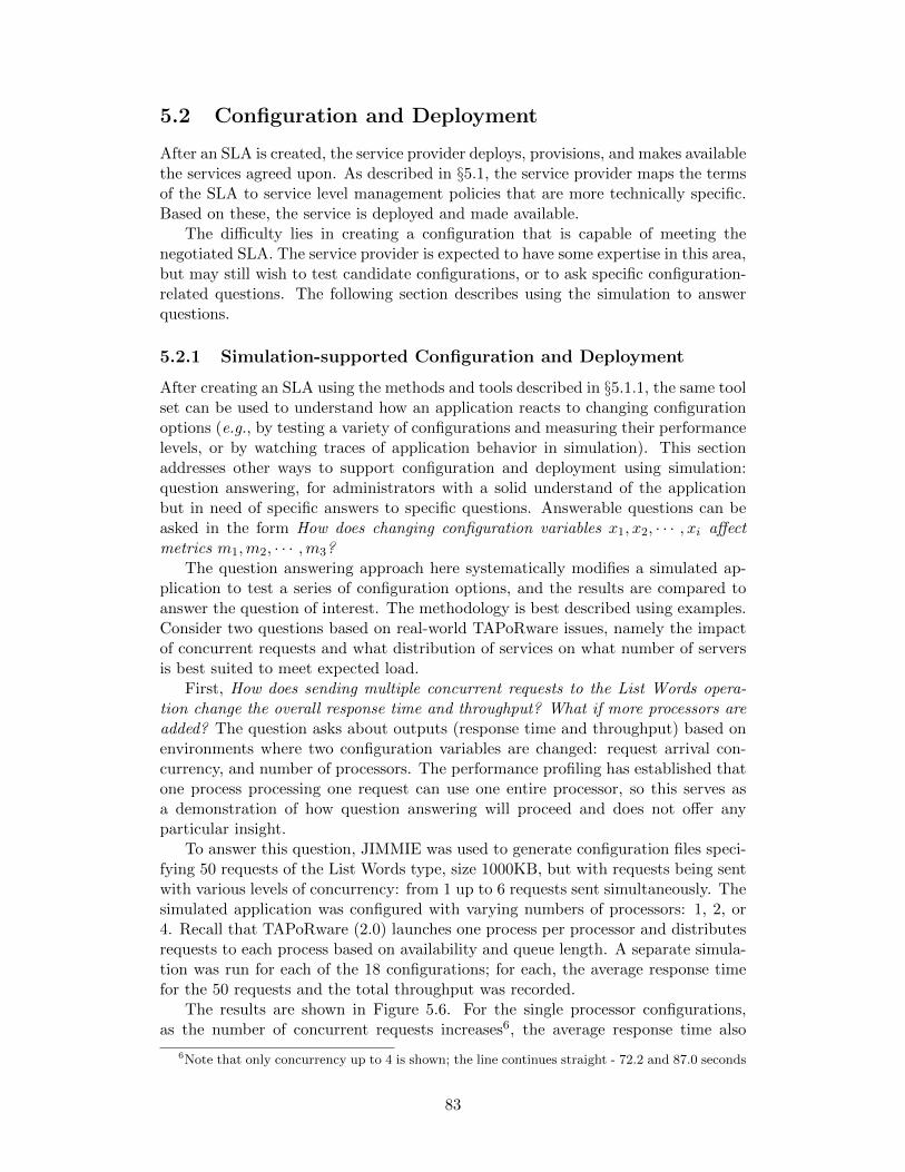
5.2 Configuration and Deployment
After an SLA is created, the service provider deploys, provisions, and makes availablethe services agreed upon. As described in §5.1, the service provider maps the termsof the SLA to service level management policies that are more technically specific.Based on these, the service is deployed and made available.
The difficulty lies in creating a configuration that is capable of meeting thenegotiated SLA. The service provider is expected to have some expertise in this area,but may still wish to test candidate configurations, or to ask specific configuration-related questions. The following section describes using the simulation to answerquestions.
5.2.1 Simulation-supported Configuration and Deployment
After creating an SLA using the methods and tools described in §5.1.1, the same toolset can be used to understand how an application reacts to changing configurationoptions (e.g., by testing a variety of configurations and measuring their performancelevels, or by watching traces of application behavior in simulation). This sectionaddresses other ways to support configuration and deployment using simulation:question answering, for administrators with a solid understand of the applicationbut in need of specific answers to specific questions. Answerable questions can beasked in the form How does changing configuration variables x1, x2, · · · , xi affectmetrics m1,m2, · · · ,m3?
The question answering approach here systematically modifies a simulated ap-plication to test a series of configuration options, and the results are compared toanswer the question of interest. The methodology is best described using examples.Consider two questions based on real-world TAPoRware issues, namely the impactof concurrent requests and what distribution of services on what number of serversis best suited to meet expected load.
First, How does sending multiple concurrent requests to the List Words opera-tion change the overall response time and throughput? What if more processors areadded? The question asks about outputs (response time and throughput) based onenvironments where two configuration variables are changed: request arrival con-currency, and number of processors. The performance profiling has established thatone process processing one request can use one entire processor, so this serves asa demonstration of how question answering will proceed and does not offer anyparticular insight.
To answer this question, JIMMIE was used to generate configuration files speci-fying 50 requests of the List Words type, size 1000KB, but with requests being sentwith various levels of concurrency: from 1 up to 6 requests sent simultaneously. Thesimulated application was configured with varying numbers of processors: 1, 2, or4. Recall that TAPoRware (2.0) launches one process per processor and distributesrequests to each process based on availability and queue length. A separate simula-tion was run for each of the 18 configurations; for each, the average response timefor the 50 requests and the total throughput was recorded.
The results are shown in Figure 5.6. For the single processor configurations,as the number of concurrent requests increases6, the average response time also
6Note that only concurrency up to 4 is shown; the line continues straight - 72.2 and 87.0 seconds
83
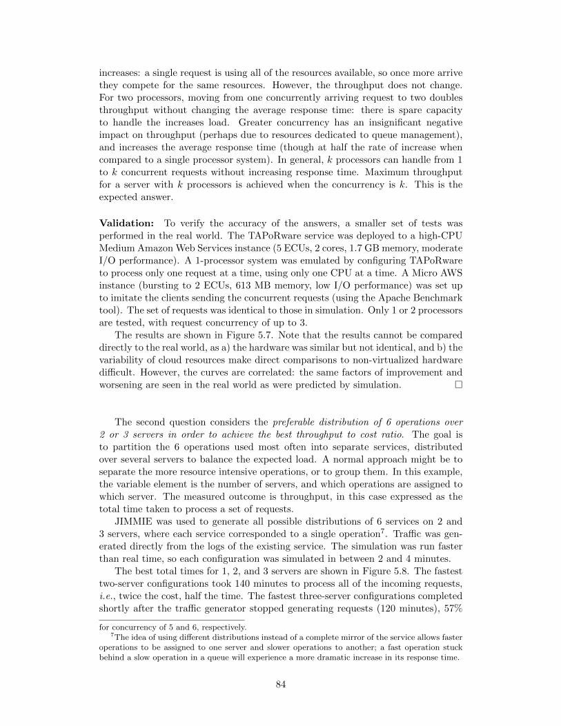
increases: a single request is using all of the resources available, so once more arrivethey compete for the same resources. However, the throughput does not change.For two processors, moving from one concurrently arriving request to two doublesthroughput without changing the average response time: there is spare capacityto handle the increases load. Greater concurrency has an insignificant negativeimpact on throughput (perhaps due to resources dedicated to queue management),and increases the average response time (though at half the rate of increase whencompared to a single processor system). In general, k processors can handle from 1to k concurrent requests without increasing response time. Maximum throughputfor a server with k processors is achieved when the concurrency is k. This is theexpected answer.
Validation: To verify the accuracy of the answers, a smaller set of tests wasperformed in the real world. The TAPoRware service was deployed to a high-CPUMedium Amazon Web Services instance (5 ECUs, 2 cores, 1.7 GB memory, moderateI/O performance). A 1-processor system was emulated by configuring TAPoRwareto process only one request at a time, using only one CPU at a time. A Micro AWSinstance (bursting to 2 ECUs, 613 MB memory, low I/O performance) was set upto imitate the clients sending the concurrent requests (using the Apache Benchmarktool). The set of requests was identical to those in simulation. Only 1 or 2 processorsare tested, with request concurrency of up to 3.
The results are shown in Figure 5.7. Note that the results cannot be compareddirectly to the real world, as a) the hardware was similar but not identical, and b) thevariability of cloud resources make direct comparisons to non-virtualized hardwaredifficult. However, the curves are correlated: the same factors of improvement andworsening are seen in the real world as were predicted by simulation. �
The second question considers the preferable distribution of 6 operations over2 or 3 servers in order to achieve the best throughput to cost ratio. The goal isto partition the 6 operations used most often into separate services, distributedover several servers to balance the expected load. A normal approach might be toseparate the more resource intensive operations, or to group them. In this example,the variable element is the number of servers, and which operations are assigned towhich server. The measured outcome is throughput, in this case expressed as thetotal time taken to process a set of requests.
JIMMIE was used to generate all possible distributions of 6 services on 2 and3 servers, where each service corresponded to a single operation7. Traffic was gen-erated directly from the logs of the existing service. The simulation was run fasterthan real time, so each configuration was simulated in between 2 and 4 minutes.
The best total times for 1, 2, and 3 servers are shown in Figure 5.8. The fastesttwo-server configurations took 140 minutes to process all of the incoming requests,i.e., twice the cost, half the time. The fastest three-server configurations completedshortly after the traffic generator stopped generating requests (120 minutes), 57%
for concurrency of 5 and 6, respectively.7The idea of using different distributions instead of a complete mirror of the service allows faster
operations to be assigned to one server and slower operations to another; a fast operation stuckbehind a slow operation in a queue will experience a more dramatic increase in its response time.
84
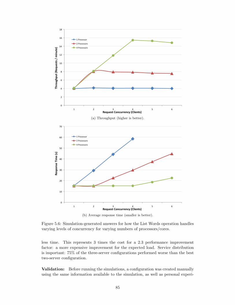
0
2
4
6
8
10
12
14
16
18
1 2 3 4 5 6
Throughp
ut (R
eque
sts / minute)
Request Concurrency (Clients)
1 Processor
2 Processors
4 Processors
(a) Throughput (higher is better).
0
10
20
30
40
50
60
70
1 2 3 4 5 6
Respon
se Tim
e (s)
Request Concurrency (Clients)
1 Processor
2 Processors
4 Processors
(b) Average response time (smaller is better).
Figure 5.6: Simulation-generated answers for how the List Words operation handlesvarying levels of concurrency for varying numbers of processors/cores.
less time. This represents 3 times the cost for a 2.3 performance improvementfactor: a more expensive improvement for the expected load. Service distributionis important: 75% of the three-server configurations performed worse than the besttwo-server configuration.
Validation: Before running the simulations, a configuration was created manuallyusing the same information available to the simulation, as well as personal experi-
85
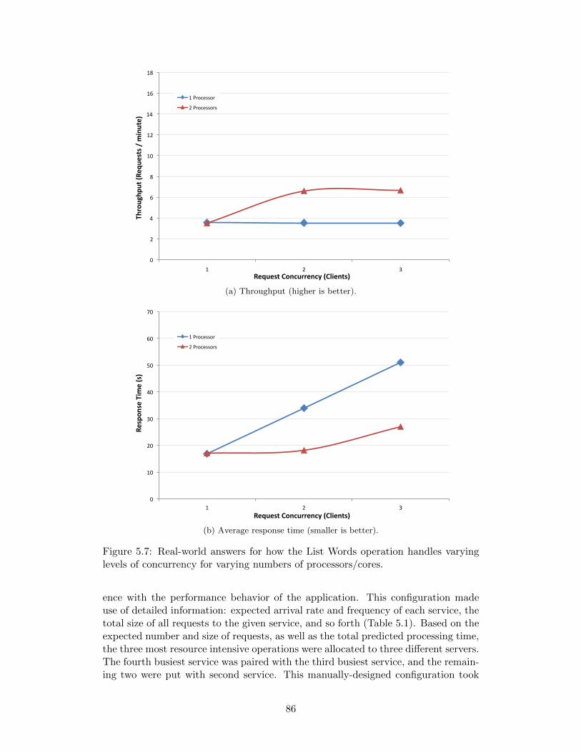
0
2
4
6
8
10
12
14
16
18
1 2 3
Throughp
ut (R
eque
sts / minute)
Request Concurrency (Clients)
1 Processor
2 Processors
(a) Throughput (higher is better).
0
10
20
30
40
50
60
70
1 2 3
Respon
se Tim
e (s)
Request Concurrency (Clients)
1 Processor
2 Processors
(b) Average response time (smaller is better).
Figure 5.7: Real-world answers for how the List Words operation handles varyinglevels of concurrency for varying numbers of processors/cores.
ence with the performance behavior of the application. This configuration madeuse of detailed information: expected arrival rate and frequency of each service, thetotal size of all requests to the given service, and so forth (Table 5.1). Based on theexpected number and size of requests, as well as the total predicted processing time,the three most resource intensive operations were allocated to three different servers.The fourth busiest service was paired with the third busiest service, and the remain-ing two were put with second service. This manually-designed configuration took
86
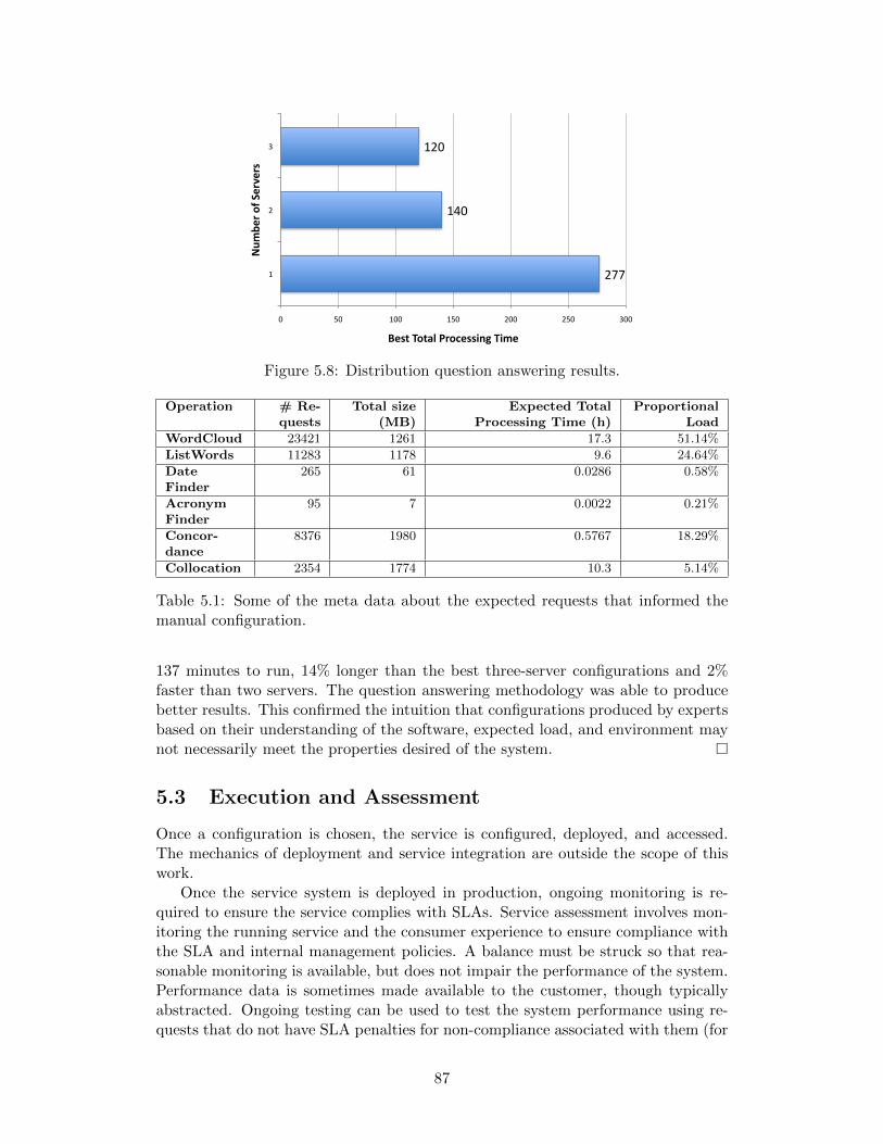
277
140
120
0 50 100 150 200 250 300
1
2
3
Best Total Processing Time
Num
ber of Servers
Figure 5.8: Distribution question answering results.
Operation # Re-quests
Total size(MB)
Expected TotalProcessing Time (h)
ProportionalLoad
WordCloud 23421 1261 17.3 51.14%
ListWords 11283 1178 9.6 24.64%
DateFinder
265 61 0.0286 0.58%
AcronymFinder
95 7 0.0022 0.21%
Concor-dance
8376 1980 0.5767 18.29%
Collocation 2354 1774 10.3 5.14%
Table 5.1: Some of the meta data about the expected requests that informed themanual configuration.
137 minutes to run, 14% longer than the best three-server configurations and 2%faster than two servers. The question answering methodology was able to producebetter results. This confirmed the intuition that configurations produced by expertsbased on their understanding of the software, expected load, and environment maynot necessarily meet the properties desired of the system. �
5.3 Execution and Assessment
Once a configuration is chosen, the service is configured, deployed, and accessed.The mechanics of deployment and service integration are outside the scope of thiswork.
Once the service system is deployed in production, ongoing monitoring is re-quired to ensure the service complies with SLAs. Service assessment involves mon-itoring the running service and the consumer experience to ensure compliance withthe SLA and internal management policies. A balance must be struck so that rea-sonable monitoring is available, but does not impair the performance of the system.Performance data is sometimes made available to the customer, though typicallyabstracted. Ongoing testing can be used to test the system performance using re-quests that do not have SLA penalties for non-compliance associated with them (for
87
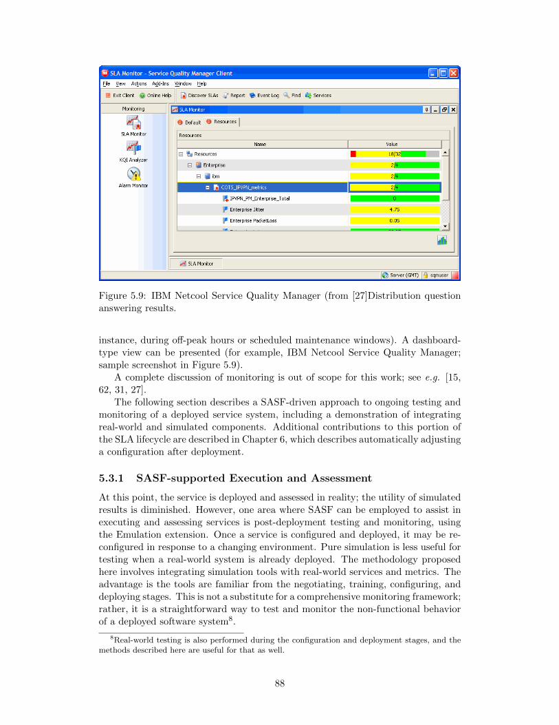
Figure 5.9: IBM Netcool Service Quality Manager (from [27]Distribution questionanswering results.
instance, during off-peak hours or scheduled maintenance windows). A dashboard-type view can be presented (for example, IBM Netcool Service Quality Manager;sample screenshot in Figure 5.9).
A complete discussion of monitoring is out of scope for this work; see e.g. [15,62, 31, 27].
The following section describes a SASF-driven approach to ongoing testing andmonitoring of a deployed service system, including a demonstration of integratingreal-world and simulated components. Additional contributions to this portion ofthe SLA lifecycle are described in Chapter 6, which describes automatically adjustinga configuration after deployment.
5.3.1 SASF-supported Execution and Assessment
At this point, the service is deployed and assessed in reality; the utility of simulatedresults is diminished. However, one area where SASF can be employed to assist inexecuting and assessing services is post-deployment testing and monitoring, usingthe Emulation extension. Once a service is configured and deployed, it may be re-configured in response to a changing environment. Pure simulation is less useful fortesting when a real-world system is already deployed. The methodology proposedhere involves integrating simulation tools with real-world services and metrics. Theadvantage is the tools are familiar from the negotiating, training, configuring, anddeploying stages. This is not a substitute for a comprehensive monitoring framework;rather, it is a straightforward way to test and monitor the non-functional behaviorof a deployed software system8.
8Real-world testing is also performed during the configuration and deployment stages, and themethods described here are useful for that as well.
88
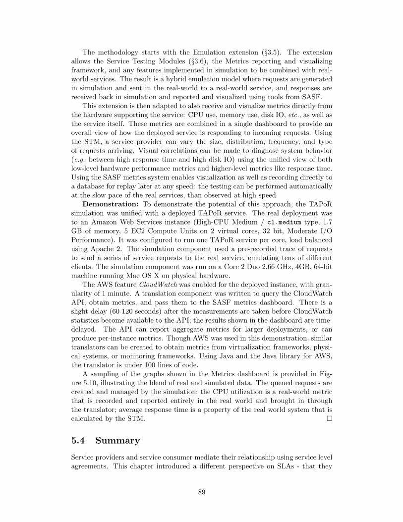
The methodology starts with the Emulation extension (§3.5). The extensionallows the Service Testing Modules (§3.6), the Metrics reporting and visualizingframework, and any features implemented in simulation to be combined with real-world services. The result is a hybrid emulation model where requests are generatedin simulation and sent in the real-world to a real-world service, and responses arereceived back in simulation and reported and visualized using tools from SASF.
This extension is then adapted to also receive and visualize metrics directly fromthe hardware supporting the service: CPU use, memory use, disk IO, etc., as well asthe service itself. These metrics are combined in a single dashboard to provide anoverall view of how the deployed service is responding to incoming requests. Usingthe STM, a service provider can vary the size, distribution, frequency, and typeof requests arriving. Visual correlations can be made to diagnose system behavior(e.g. between high response time and high disk IO) using the unified view of bothlow-level hardware performance metrics and higher-level metrics like response time.Using the SASF metrics system enables visualization as well as recording directly toa database for replay later at any speed: the testing can be performed automaticallyat the slow pace of the real services, than observed at high speed.
Demonstration: To demonstrate the potential of this approach, the TAPoRsimulation was unified with a deployed TAPoR service. The real deployment wasto an Amazon Web Services instance (High-CPU Medium / c1.medium type, 1.7GB of memory, 5 EC2 Compute Units on 2 virtual cores, 32 bit, Moderate I/OPerformance). It was configured to run one TAPoR service per core, load balancedusing Apache 2. The simulation component used a pre-recorded trace of requeststo send a series of service requests to the real service, emulating tens of differentclients. The simulation component was run on a Core 2 Duo 2.66 GHz, 4GB, 64-bitmachine running Mac OS X on physical hardware.
The AWS feature CloudWatch was enabled for the deployed instance, with gran-ularity of 1 minute. A translation component was written to query the CloudWatchAPI, obtain metrics, and pass them to the SASF metrics dashboard. There is aslight delay (60-120 seconds) after the measurements are taken before CloudWatchstatistics become available to the API; the results shown in the dashboard are time-delayed. The API can report aggregate metrics for larger deployments, or canproduce per-instance metrics. Though AWS was used in this demonstration, similartranslators can be created to obtain metrics from virtualization frameworks, physi-cal systems, or monitoring frameworks. Using Java and the Java library for AWS,the translator is under 100 lines of code.
A sampling of the graphs shown in the Metrics dashboard is provided in Fig-ure 5.10, illustrating the blend of real and simulated data. The queued requests arecreated and managed by the simulation; the CPU utilization is a real-world metricthat is recorded and reported entirely in the real world and brought in throughthe translator; average response time is a property of the real world system that iscalculated by the STM. �
5.4 Summary
Service providers and service consumer mediate their relationship using service levelagreements. This chapter introduced a different perspective on SLAs - that they
89
are lasting, cyclic documents that last as long as the interaction between a ser-vice provider and service consumers. They must be periodically reviewed and re-negotiated if necessary to match the changing business requirements or technicalproperties. Like existing SLA lifecycles, a configuration is created from the SLAand deployed; the running service is tested and monitored to ensure compliance. Itwill eventually be necessary to terminate the SLA.
This chapter described simulation-driven contributions that assist each phase ofthe lifecycle. Each was implemented in simulation and validated to produce resultsthat met the requirements; two were also tested on real-world deployments to verifytheir viability.
• A methodology, tool, and numeric representation of trade-off balance cost-benefit analysis to assist in understanding and choosing the balance betweendependent metrics. It was demonstrated that hundreds of candidate config-urations could be tested, visualized, and presented to a user who chose theirpreferred trade-offs. The tool narrowed down the candidate configurations by94%.
• A question-answering methodology and tool that assists a service provider inproducing a configuration that meets the SLA (through his or her interactionwith the tool), and in better understanding a service system generally. Theapproach was demonstrated on two questions, on both the simulation and ona real-world deployment. The question was answered with more detail thanwould be possible without a simulation; for the tests feasible in the real worldenvironment, it was shown that the answers were the same as the simulation-produced answers.
• A monitoring and assessment tool that integrates simulated components withreal-world services to use the flexible and powerful service testing modulesand the metrics/dashboard framework of SASF to produce, visualize, andstore real-world data. The tool was demonstrated exercising a real-world de-ployment of TAPoR and visualizing simulation-generated metrics alongsidereal-world metrics.
The primary threat to validity is these simulation-driven approaches have notbeen validated in user studies that demonstrate that SLAs, configurations, andassessments are actually producing results that satisfy users. Though the method-ologies and tools meet the derived requirements (more co-created value, more infor-mation sharing, analysis of trade-offs), and are shown to perform as designed, thelast step of a user study is not taken.
90
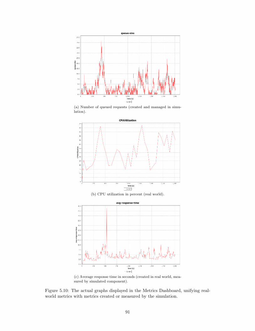
(a) Number of queued requests (created and managed in simu-lation).
(b) CPU utilization in percent (real world).
(c) Average response time in seconds (created in real world, mea-sured by simulated component).
Figure 5.10: The actual graphs displayed in the Metrics Dashboard, unifying real-world metrics with metrics created or measured by the simulation.
91
Chapter 6
Autonomic Configuration usingSimulation
Chapter Contents
6.1 State-Transition Model . . . . . . . . 93
6.1.1 States . . . . . . . . . . . . . . 93
6.1.2 Transitions . . . . . . . . . . . 96
6.1.3 Expert-driven Model-Construction . . . . . . . . . . 97
6.2 Autonomic Management . . . . . . . 99
6.2.1 Evaluation in Simulation . . . . 101
6.2.2 Evaluation in Reality . . . . . . 103
6.3 Systematic Exploration of the StateSpace . . . . . . . . . . . . . . . . . 106
6.3.1 Exploration-driven Model Con-struction . . . . . . . . . . . . . 107
6.3.2 Evaluation . . . . . . . . . . . . 108
6.3.3 Data Volume and Granularity . 110
6.4 Threats to Validity and Shortcomings112
6.5 Summary . . . . . . . . . . . . . . . 113
Configuration management is acomplex task, even for experienced sys-tem administrators, which makes self-managing systems a desirable contribu-tion [32, 48, 56]. This chapter describesa novel approach to self-managing sys-tems, implemented as an autonomicconfiguration tool.
The self-configuration decision-makingmethodology uses a simulation model ofthe subject system and systematicallyexecutes it in order to collect examplesof its expected behavior under differ-ent conditions of load, configuration andSLA constraints. The motivating re-configuration scenarios involve adaptingthe number of servers on which the sys-tem services are deployed.
From these examples of behavior, abehavioral state-transition model is created. The metrics recorded in each moni-toring step are discretized to produce a more coarse-grained representation of therecorded data, which is clustered into classes, each of which represents a behav-ioral state. Two states are related with a transition between them if an instance ofthe source state is followed in time by an instance of the destination state. Thesetransitions represent changes in demand (when the system load metrics increase)or changes in the system configuration (when the system configuration changes).Precise definitions of the states and transitions, and the details of how the completemodel is created, are provided in §6.1.
The autonomic manager (§6.2) monitors the system at run-time, taking periodicsnapshots of its load and configuration. This data enables it to identify in which ofthe behavioral states it is, tracking the progress of the system through the state-transition model. When the system is in a state known to violate (or to potentially
92
lead to violations of) its SLA, a search for a configuration change transition (or aseries thereof) that will lead to a satisfactory state is initiated. The required changesare executed; that is, the subject system is reconfigured and monitoring resumes.
To demonstrate and validate the methodology, a state model is created usingTAPoRsim (§4.4). An autonomic manager is implemented and verified in sim-ulation, then TAPoRware is deployed to a cloud computing environment and theautonomic manager is tested in a real-world environment. §6.2.1 and §6.2.2 describethe experiment and demonstrate a decision model generated entirely in simulationcan be used to make accurate changes to a real-world application.§6.3 examines the process of generating the state-transition model in more detail.
The experiments used for verification use states gleaned from the simulation whileit is being exercised by an expert user. The most expensive part of the process isthe involvement of an expert. An alteration to the methodology involves exercisingthe simulation automatically and systematically, in an attempt to cover all feasiblestates. To test this approach, the performance of the autonomic manager is testedin two scenarios: one where the expert-generated traces are used to construct thestate-transition model, and a second where traces from thousands of systematicallyconfigured simulations are used instead.
The nature of the state-transition model and the attempt to cover “all feasiblestates” raises questions about how much data is needed to produce an autonomicmanager of sufficient quality. The volume and granularity of data is important tounderstand - the potential issue is that if too many states are required to accuratelyrepresent the system, problems of scale will arise. The usefulness of the autonomicmanager with even a small number of states is demonstrated in §6.3.3.
6.1 State-Transition Model
The decision model used to inform the autonomic manager is a set of states andtransitions between them. This section defines states and transitions, and discusseshow the model is obtained by monitoring a simulation.
6.1.1 States
A snapshot is a tuple of metrics recorded within a period of time that show thebehavior of the application at a moment in time. For each snapshot, a snapshotdescriptor is calculated and recorded. A snapshot descriptor has three parts. Thefirst part defines the state’s compliance with the SLA: Satisfactory, Unsatisfactory,or Boundary (the SUB metric). Boundary states are states which meet the SLA,but which have transitions to unsatisfactory states1. The second element is a setof configuration-related parameters, i.e., a set of metrics related to the currentenvironment (number of incoming requests, etc.). Finally the third value of thesnapshop triple is a set of performance metrics:
S = 〈(S | U | B), 〈Configuration〉, 〈Environment〉, 〈Metrics〉〉
The internal structure of the snapshot descriptor, namely the actual metrics in-cluded in the configuration-parameter and performance-metrics set, depends on the
1Note that this value is not static: the same simulation data with a different SLA will producedifferent states as the SUB metric may change.
93
1. SUB metric
2. Configuration
(a) Number of servers.
(b) Number of processors.
(c) Limit on concurrent requests
3. Environment
(a) Requests / 5 seconds (sliding window)
(b) Request size / 5 seconds (sliding window)
4. Performance
(a) Total queued requests
(b) CPU utilization (over all processors)
(c) Average response time (rolling)
(d) Response time standard deviation
(e) Largest queue at single servers
(f) Highest CPU utilization at single server
(g) Smallest queue at single server
(h) Lowest CPU utilization at single server
(i) Throughput (responses / minute)
(j) Memory footprint
Table 6.1: The elements of a snapshot descriptor for TAPoRsim.
subject system. The challenge is to identify a tuple that includes measurable infor-mation sufficient to characterize the performance of the system without includingextraneous information. The snapshot descriptor used for TAPoRsim is shown inTable 6.1.
To control the size of the state space, snapshot descriptors are clustered intoequivalence classes, called states. The snapshot descriptors within each state are“similar enough”, in that there is no significant difference in their environment,performance, or configuration metrics2. Each state is annotated with a cost, thecost of the cheapest configuration of all its snapshot descriptors. The function usedto determine the configuration costs could be the cost of hardware, the cost ofmaintenance, the “green-ness”, etc.
Whether two values of a performance metric are “similar enough” depends onthe level of precision/abstraction at which metrics are examined. At the lowestlevel of abstraction, any variation in any metric is considered a change. If themetrics involved are measured using real numbers (and not restricted to a range ofintegers), the state space is theoretically infinite. To restrict the size of the statespace while still producing meaningful results, the ranges of values are discretizedinto “windows” where all values within a window are considered equal to each other.For enumerated performance metrics, each enumerated value defines a “window”;
2Note that the SUB metric is ignored in the clustering process.
94

for example, the SUB metric has 3 possible values and has window size 3. Fornumeric metrics, the size of the window is chosen to give the desired number ofwindows and therefore the desired state space, while remaining appropriate for thatmetric. Three different discretization strategies are defined and implemented:
1. A fixed window size based on the theoretical range of values. For example,average response time can range from 0 seconds to 30 seconds (the timeoutpoint). The window size is then 30 seconds
desired # of windows .
2. A fixed window size based on the actual or expected range of values. Based onthe collected simulation data, the actual range of observed values is dividedby the desired number of windows, to produce the window size. For example,the average response time might actually range from .2 to 5.5 seconds, so
5.5−.2 secondsdesired # of windows .
3. A window size chosen to ensure an equal number of values in each window. Ifk = # of values
desired # of windows , then the first k values make up the first window, thenext k values make up the second, and so on.
The granularity and accuracy of the model determines the size of the state spaceand the eventual performance of the autonomic manager. If the window size is toolarge, it is not possible to understand what is actually happening in the applicationat each point in time, since one window many contain significantly different snapshotdescriptors. If the window size is too small, the state space will be larger and asthe number of transitions increases, the computation time involved in analyzing thepossible future alternatives will also increase. To avoid both of these shortcomingswhen deciding on a window, one can empirically test a variety of window sizesand observe whether the resulting equivalence classes contain sufficiently similarsimulation metrics. In parallel, one can calculate theoretical state size, based on thenumber of windows resulting from the chosen sizes, and ensure it is acceptable.
Once the number of windows for each metric wm is decided, if d is the numberof metrics included in the descriptor, then the state space size is the product of thewindow size of each descriptor as follows:
State Space Size =
d∏n=1
w[n]
or
State Space Size =
d∏n=1
r[n]
ws[n]
For example, consider a snapshot descriptor that includes only the SUB metric(w1 = 3), a CPU utilization metric, and a memory usage metric. CPU utilizationranges from 0-100 (percent); with a window size of 5, there are 20 windowsw2 =1005 = 20. In the example, memory usage ranges from 0-4096 (MB); with a window
size of 512, there are 8 windows. w3 = 4096512 = 8. The theoretical state space for the
example is therefore 3× 20× 8 = 480.The actual number of states achievable in practice is less than this theoretical
maximum, as some states are not possible in reality. For example, a snapshot that
95
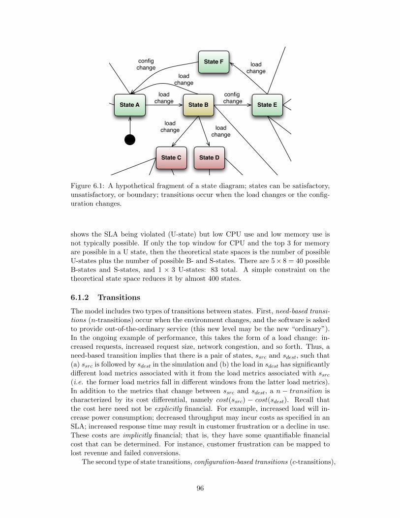
State Bconfig change
State ADescriptor: {Satisfactory, 8, 8, 16, d27, 64, 100, 1045, 4, 2129, 1400, 2400}
loadchange
State E
State C
State Aload
change
loadchange
loadchange
State D
configchange
State F loadchange
Figure 6.1: A hypothetical fragment of a state diagram; states can be satisfactory,unsatisfactory, or boundary; transitions occur when the load changes or the config-uration changes.
shows the SLA being violated (U-state) but low CPU use and low memory use isnot typically possible. If only the top window for CPU and the top 3 for memoryare possible in a U state, then the theoretical state spaces is the number of possibleU-states plus the number of possible B- and S-states. There are 5× 8 = 40 possibleB-states and S-states, and 1 × 3 U-states: 83 total. A simple constraint on thetheoretical state space reduces it by almost 400 states.
6.1.2 Transitions
The model includes two types of transitions between states. First, need-based transi-tions (n-transitions) occur when the environment changes, and the software is askedto provide out-of-the-ordinary service (this new level may be the new “ordinary”).In the ongoing example of performance, this takes the form of a load change: in-creased requests, increased request size, network congestion, and so forth. Thus, aneed-based transition implies that there is a pair of states, ssrc and sdest, such that(a) ssrc is followed by sdest in the simulation and (b) the load in sdest has significantlydifferent load metrics associated with it from the load metrics associated with ssrc(i.e. the former load metrics fall in different windows from the latter load metrics).In addition to the metrics that change between ssrc and sdest, a n − transition ischaracterized by its cost differential, namely cost(ssrc) − cost(sdest). Recall thatthe cost here need not be explicitly financial. For example, increased load will in-crease power consumption; decreased throughput may incur costs as specified in anSLA; increased response time may result in customer frustration or a decline in use.These costs are implicitly financial; that is, they have some quantifiable financialcost that can be determined. For instance, customer frustration can be mapped tolost revenue and failed conversions.
The second type of state transitions, configuration-based transitions (c-transitions),
96
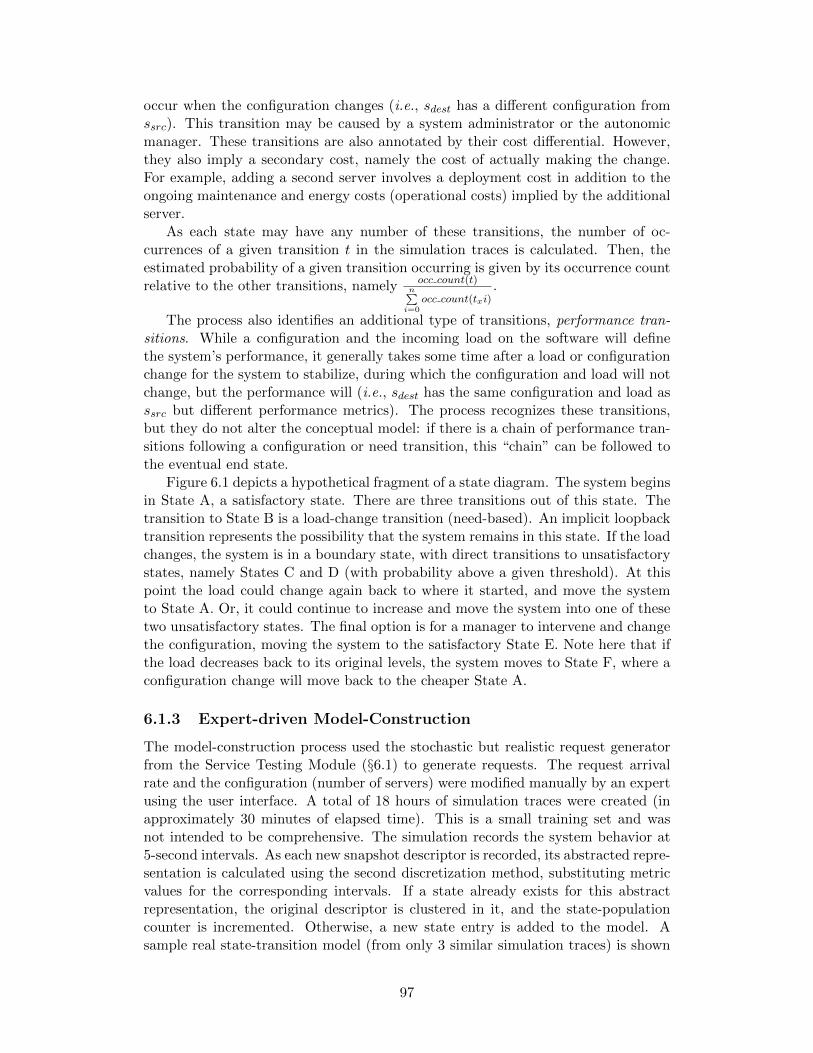
occur when the configuration changes (i.e., sdest has a different configuration fromssrc). This transition may be caused by a system administrator or the autonomicmanager. These transitions are also annotated by their cost differential. However,they also imply a secondary cost, namely the cost of actually making the change.For example, adding a second server involves a deployment cost in addition to theongoing maintenance and energy costs (operational costs) implied by the additionalserver.
As each state may have any number of these transitions, the number of oc-currences of a given transition t in the simulation traces is calculated. Then, theestimated probability of a given transition occurring is given by its occurrence countrelative to the other transitions, namely occ count(t)
n∑i=0
occ count(txi).
The process also identifies an additional type of transitions, performance tran-sitions. While a configuration and the incoming load on the software will definethe system’s performance, it generally takes some time after a load or configurationchange for the system to stabilize, during which the configuration and load will notchange, but the performance will (i.e., sdest has the same configuration and load asssrc but different performance metrics). The process recognizes these transitions,but they do not alter the conceptual model: if there is a chain of performance tran-sitions following a configuration or need transition, this “chain” can be followed tothe eventual end state.
Figure 6.1 depicts a hypothetical fragment of a state diagram. The system beginsin State A, a satisfactory state. There are three transitions out of this state. Thetransition to State B is a load-change transition (need-based). An implicit loopbacktransition represents the possibility that the system remains in this state. If the loadchanges, the system is in a boundary state, with direct transitions to unsatisfactorystates, namely States C and D (with probability above a given threshold). At thispoint the load could change again back to where it started, and move the systemto State A. Or, it could continue to increase and move the system into one of thesetwo unsatisfactory states. The final option is for a manager to intervene and changethe configuration, moving the system to the satisfactory State E. Note here that ifthe load decreases back to its original levels, the system moves to State F, where aconfiguration change will move back to the cheaper State A.
6.1.3 Expert-driven Model-Construction
The model-construction process used the stochastic but realistic request generatorfrom the Service Testing Module (§6.1) to generate requests. The request arrivalrate and the configuration (number of servers) were modified manually by an expertusing the user interface. A total of 18 hours of simulation traces were created (inapproximately 30 minutes of elapsed time). This is a small training set and wasnot intended to be comprehensive. The simulation records the system behavior at5-second intervals. As each new snapshot descriptor is recorded, its abstracted repre-sentation is calculated using the second discretization method, substituting metricvalues for the corresponding intervals. If a state already exists for this abstractrepresentation, the original descriptor is clustered in it, and the state-populationcounter is incremented. Otherwise, a new state entry is added to the model. Asample real state-transition model (from only 3 similar simulation traces) is shown
97
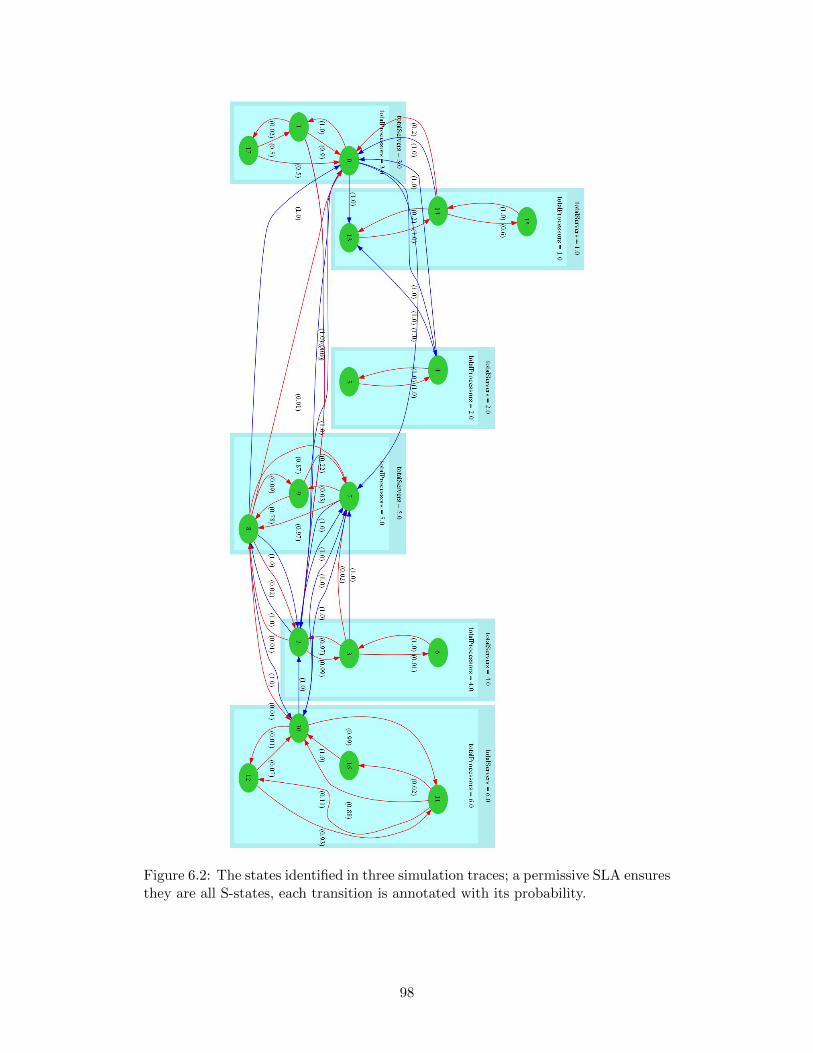
Figure 6.2: The states identified in three simulation traces; a permissive SLA ensuresthey are all S-states, each transition is annotated with its probability.
98
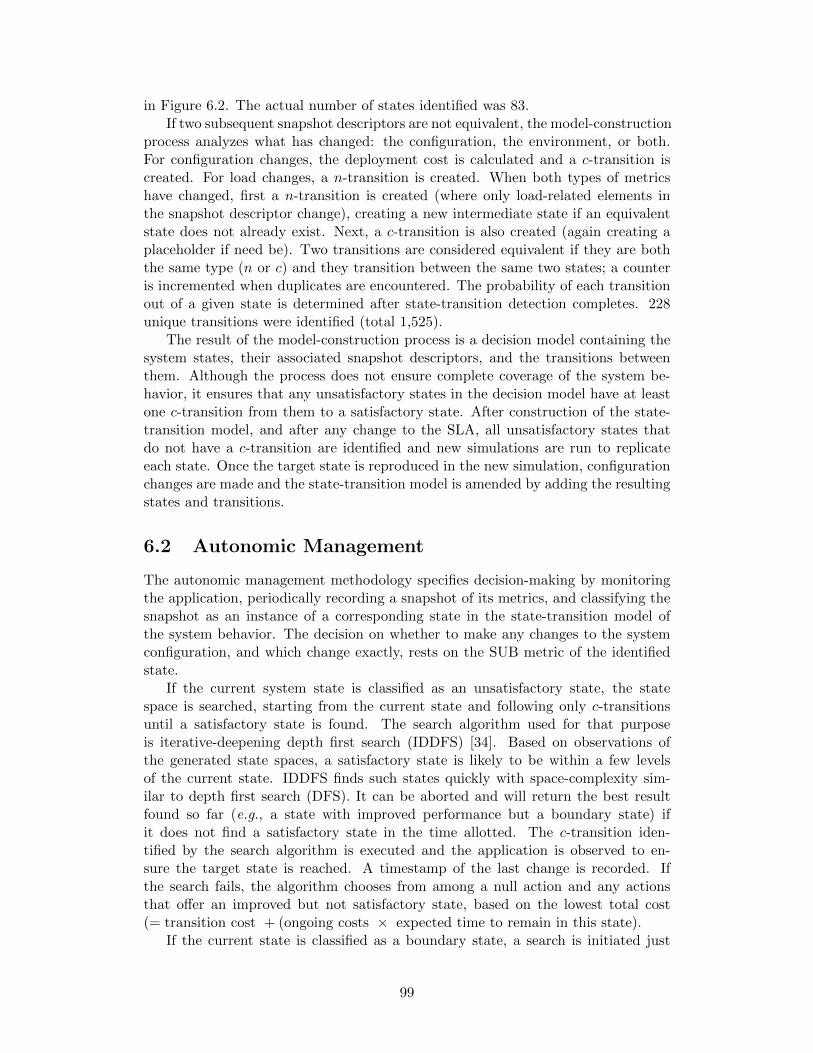
in Figure 6.2. The actual number of states identified was 83.If two subsequent snapshot descriptors are not equivalent, the model-construction
process analyzes what has changed: the configuration, the environment, or both.For configuration changes, the deployment cost is calculated and a c-transition iscreated. For load changes, a n-transition is created. When both types of metricshave changed, first a n-transition is created (where only load-related elements inthe snapshot descriptor change), creating a new intermediate state if an equivalentstate does not already exist. Next, a c-transition is also created (again creating aplaceholder if need be). Two transitions are considered equivalent if they are boththe same type (n or c) and they transition between the same two states; a counteris incremented when duplicates are encountered. The probability of each transitionout of a given state is determined after state-transition detection completes. 228unique transitions were identified (total 1,525).
The result of the model-construction process is a decision model containing thesystem states, their associated snapshot descriptors, and the transitions betweenthem. Although the process does not ensure complete coverage of the system be-havior, it ensures that any unsatisfactory states in the decision model have at leastone c-transition from them to a satisfactory state. After construction of the state-transition model, and after any change to the SLA, all unsatisfactory states thatdo not have a c-transition are identified and new simulations are run to replicateeach state. Once the target state is reproduced in the new simulation, configurationchanges are made and the state-transition model is amended by adding the resultingstates and transitions.
6.2 Autonomic Management
The autonomic management methodology specifies decision-making by monitoringthe application, periodically recording a snapshot of its metrics, and classifying thesnapshot as an instance of a corresponding state in the state-transition model ofthe system behavior. The decision on whether to make any changes to the systemconfiguration, and which change exactly, rests on the SUB metric of the identifiedstate.
If the current system state is classified as an unsatisfactory state, the statespace is searched, starting from the current state and following only c-transitionsuntil a satisfactory state is found. The search algorithm used for that purposeis iterative-deepening depth first search (IDDFS) [34]. Based on observations ofthe generated state spaces, a satisfactory state is likely to be within a few levelsof the current state. IDDFS finds such states quickly with space-complexity sim-ilar to depth first search (DFS). It can be aborted and will return the best resultfound so far (e.g., a state with improved performance but a boundary state) ifit does not find a satisfactory state in the time allotted. The c-transition iden-tified by the search algorithm is executed and the application is observed to en-sure the target state is reached. A timestamp of the last change is recorded. Ifthe search fails, the algorithm chooses from among a null action and any actionsthat offer an improved but not satisfactory state, based on the lowest total cost(= transition cost + (ongoing costs × expected time to remain in this state).
If the current state is classified as a boundary state, a search is initiated just
99
4 Servers
5 Servers
6 Servers Manual
Autonomic
0
50
100
150
200
250
Respon
se Tim
e (s)
Cost
Figure 6.3: The performance / cost trade-offs for the linearly increasing data set insimulation.
as for the unsatisfactory state; however, the configuration changes implied by thetransition sequence are only executed if the identified target state is superior to thecurrent boundary state (an S-state, or a B-state with improved performance and/orlower cost).
If the current state is classified as a satisfactory state, a search for a path of c-transitions that leads to another satisfactory state is initiated. If a path is identified,it is executed if (a) the time elapsed since the last change is sufficient (for a definedthreshold; 5 minutes in the implementation, but configurable), and (b) the new stateis cheaper than the current state. This will remove over-provisioned resources whileavoiding “churn” of repeated adds/removes for performance levels at or near SLAlevels.
If the SLA changes, each of the recorded snapshot descriptors is revisited torecalculate its associated SUB metric. If after this process the system is found tobe in an unsatisfactory state, the adaptation algorithm above is invoked in order totransition to a satisfactory state. Recall that every unsatisfactory state must have atleast one c-transition to a satisfactory state; if new unsatisfactory states are addedas a result of the SLA change, this requirement might be violated and additionalsimulations may be required to update the state-transition model.
Depending on the completeness of the simulation-generated state-transition model,the running application may encounter states not yet seen in the simulation tracesor may transition to existing states via previously undetected transitions. In thesecases, the model-construction algorithm adds the appropriate states and transitionsto the model. If the new state is unsatisfactory, there is no strategy to adapt theconfiguration. The current implementation identifies this situation and notifies anadministrator. The methodology specifies that ultimately an update to the state-transition model must be scheduled, but the immediate reaction is to use a modifiedstate equivalence function to identify similar states that violate the SLA in the sameway and use one of their c-transitions to attempt a move to a satisfactory state.
100

Config Resp. Time Cost Performance
4 192.59 0.0% 0.0%
5 43.39 15.8% 77.5%
6 2.95 34.4% 98.5%
Manual 2.45 -43.1% 98.7%
Autonomic 30.17 -60.9% 84.3%
Table 6.2: Cost and performance metrics (and improvements) for 6 configurationsand the linearly increasing data set in simulation.
6.2.1 Evaluation in Simulation
To demonstrate and test the methodology, an autonomic manager was implemented,comprising three components:
1. TAPoRsim and the SASF framework, which generate simulation traces;
2. Decision model constructor, which produces a state-transition model fromsimulation traces;
3. Autonomic decision maker, which uses the decision model to make re-configurationdecisions.
The simulation traces and the decision model are produced offline in advanceof the deployment of the autonomic decision maker; for this evaluation, the statemodel described in §6.1.3 was used. The autonomic decision maker is built on theSASF framework and runs in simulation. It uses a MetricListener implementationto monitor the running simulation, and modifies the configuration of the simulatedapplication using the provided API.
The evaluation is based on monitoring and adapting the simulated version of theapplication by adding or removing servers in response to changing request loads.The service level objective was a very ambitious response time of 5 seconds, with amaximum queue length of 20 requests (recall this is not a simple web request, butCPU-intensive analysis of texts up to 7 MB in size).
Two pre-recorded but pseudo-randomly generated series of requests served astest input for the experiments. These sets of requests were not used or known whenconstructing the state model. For the first, an individual not familiar with thisproject generated 3 hours of request traffic using the modifiable stochastic requestgenerator (variable data set). The second used a linearly increasing load, from 500to 70,000 requests per hour, increasing by 600 requests a minute. The requests (size,type, and time) were recorded and used as input to the simulated application in 5different conditions as follows:
• In the first three conditions, a fixed number of servers (4, 5, and 6, respectively)was used, reflecting static configurations, with no configuration changes madeat run time.
• For the fourth condition, an expert user monitored performance metrics us-ing the visualization dashboard and added or removed servers as he deemedappropriate (from 1 server to a maximum of 6 servers). The expert user had
101
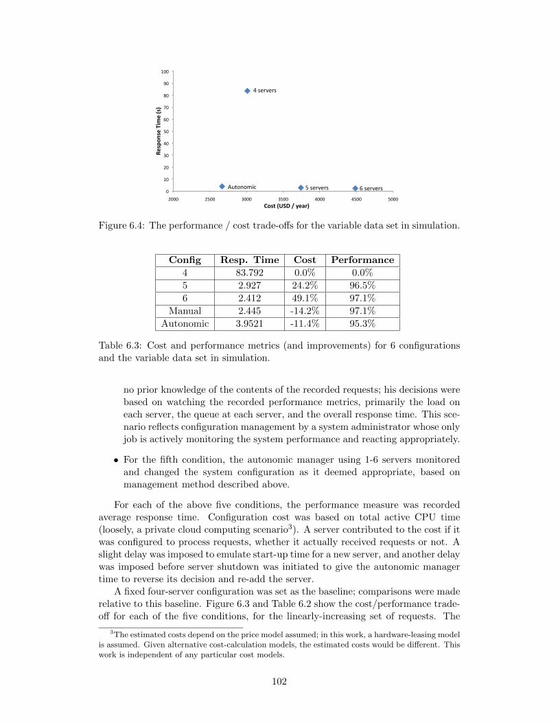
4 servers
5 servers 6 servers Autonomic 0
10
20
30
40
50
60
70
80
90
100
2000 2500 3000 3500 4000 4500 5000
Respon
se Tim
e (s)
Cost (USD / year)
Figure 6.4: The performance / cost trade-offs for the variable data set in simulation.
Config Resp. Time Cost Performance
4 83.792 0.0% 0.0%
5 2.927 24.2% 96.5%
6 2.412 49.1% 97.1%
Manual 2.445 -14.2% 97.1%
Autonomic 3.9521 -11.4% 95.3%
Table 6.3: Cost and performance metrics (and improvements) for 6 configurationsand the variable data set in simulation.
no prior knowledge of the contents of the recorded requests; his decisions werebased on watching the recorded performance metrics, primarily the load oneach server, the queue at each server, and the overall response time. This sce-nario reflects configuration management by a system administrator whose onlyjob is actively monitoring the system performance and reacting appropriately.
• For the fifth condition, the autonomic manager using 1-6 servers monitoredand changed the system configuration as it deemed appropriate, based onmanagement method described above.
For each of the above five conditions, the performance measure was recordedaverage response time. Configuration cost was based on total active CPU time(loosely, a private cloud computing scenario3). A server contributed to the cost if itwas configured to process requests, whether it actually received requests or not. Aslight delay was imposed to emulate start-up time for a new server, and another delaywas imposed before server shutdown was initiated to give the autonomic managertime to reverse its decision and re-add the server.
A fixed four-server configuration was set as the baseline; comparisons were maderelative to this baseline. Figure 6.3 and Table 6.2 show the cost/performance trade-off for each of the five conditions, for the linearly-increasing set of requests. The
3The estimated costs depend on the price model assumed; in this work, a hardware-leasing modelis assumed. Given alternative cost-calculation models, the estimated costs would be different. Thiswork is independent of any particular cost models.
102
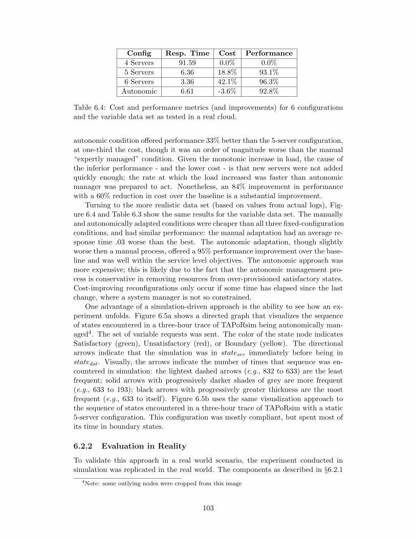
Config Resp. Time Cost Performance
4 Servers 91.59 0.0% 0.0%
5 Servers 6.36 18.8% 93.1%
6 Servers 3.36 42.1% 96.3%
Autonomic 6.61 -3.6% 92.8%
Table 6.4: Cost and performance metrics (and improvements) for 6 configurationsand the variable data set as tested in a real cloud.
autonomic condition offered performance 33% better than the 5-server configuration,at one-third the cost, though it was an order of magnitude worse than the manual“expertly managed” condition. Given the monotonic increase in load, the cause ofthe inferior performance - and the lower cost - is that new servers were not addedquickly enough; the rate at which the load increased was faster than autonomicmanager was prepared to act. Nonetheless, an 84% improvement in performancewith a 60% reduction in cost over the baseline is a substantial improvement.
Turning to the more realistic data set (based on values from actual logs), Fig-ure 6.4 and Table 6.3 show the same results for the variable data set. The manuallyand autonomically adapted conditions were cheaper than all three fixed-configurationconditions, and had similar performance: the manual adaptation had an average re-sponse time .03 worse than the best. The autonomic adaptation, though slightlyworse then a manual process, offered a 95% performance improvement over the base-line and was well within the service level objectives. The autonomic approach wasmore expensive; this is likely due to the fact that the autonomic management pro-cess is conservative in removing resources from over-provisioned satisfactory states.Cost-improving reconfigurations only occur if some time has elapsed since the lastchange, where a system manager is not so constrained.
One advantage of a simulation-driven approach is the ability to see how an ex-periment unfolds. Figure 6.5a shows a directed graph that visualizes the sequenceof states encountered in a three-hour trace of TAPoRsim being autonomically man-aged4. The set of variable requests was sent. The color of the state node indicatesSatisfactory (green), Unsatisfactory (red), or Boundary (yellow). The directionalarrows indicate that the simulation was in statesrc immediately before being instatedst. Visually, the arrows indicate the number of times that sequence was en-countered in simulation: the lightest dashed arrows (e.g., 832 to 633) are the leastfrequent; solid arrows with progressively darker shades of grey are more frequent(e.g., 633 to 193); black arrows with progressively greater thickness are the mostfrequent (e.g., 633 to itself). Figure 6.5b uses the same visualization approach tothe sequence of states encountered in a three-hour trace of TAPoRsim with a static5-server configuration. This configuration was mostly compliant, but spent most ofits time in boundary states.
6.2.2 Evaluation in Reality
To validate this approach in a real world scenario, the experiment conducted insimulation was replicated in the real world. The components as described in §6.2.1
4Note: some outlying nodes were cropped from this image
103
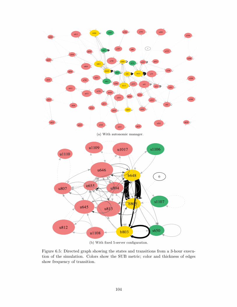
(a) With autonomic manager.
(b) With fixed 5-server configuration.
Figure 6.5: Directed graph showing the states and transitions from a 3-hour execu-tion of the simulation. Colors show the SUB metric; color and thickness of edgesshow frequency of transition.
104
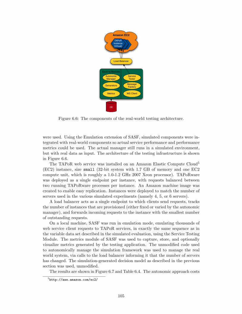
Amazon EC2
TAPoR Instance (Virtual)
Load Balancer
Metrics
DB
Generators
Autonomic Manager
Existing Modules
Message Factory
Service Tester
WS Client
Figure 6.6: The components of the real-world testing architecture.
were used. Using the Emulation extension of SASF, simulated components were in-tegrated with real-world components so actual service performance and performancemetrics could be used. The actual manager still runs in a simulated environment,but with real data as input. The architecture of the testing infrastructure is shownin Figure 6.6.
The TAPoR web service was installed on an Amazon Elastic Compute Cloud5
(EC2) instance, size small (32-bit system with 1.7 GB of memory and one EC2compute unit, which is roughly a 1.0-1.2 GHz 2007 Xeon processor). TAPoRwarewas deployed as a single endpoint per instance, with requests balanced betweentwo running TAPoRware processes per instance. An Amazon machine image wascreated to enable easy replication. Instances were deployed to match the number ofservers used in the various simulated experiments (namely 4, 5, or 6 servers).
A load balancer acts as a single endpoint to which clients send requests, tracksthe number of instances that are provisioned (either fixed or varied by the autonomicmanager), and forwards incoming requests to the instance with the smallest numberof outstanding requests.
On a local machine, SASF was run in emulation mode, emulating thousands ofweb service client requests to TAPoR services, in exactly the same sequence as inthe variable data set described in the simulated evaluation, using the Service TestingModule. The metrics module of SASF was used to capture, store, and optionallyvisualize metrics generated by the testing application. The unmodified code usedto autonomically manage the simulation framework was used to manage the realworld system, via calls to the load balancer informing it that the number of servershas changed. The simulation-generated decision model as described in the previoussection was used, unmodified.
The results are shown in Figure 6.7 and Table 6.4. The autonomic approach costs
5http://aws.amazon.com/ec2/
105
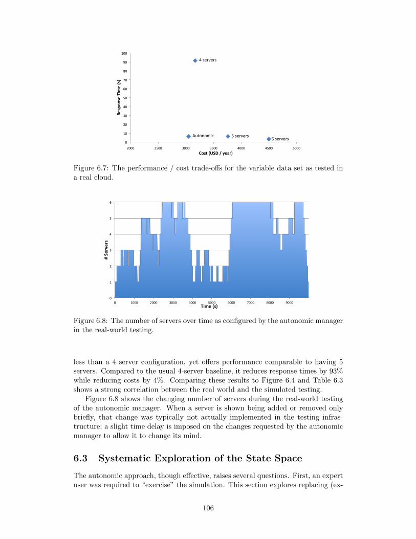
4 servers
5 servers 6 servers
Autonomic 0
10
20
30
40
50
60
70
80
90
100
2000 2500 3000 3500 4000 4500 5000
Respon
se Tim
e (s)
Cost (USD / year)
Figure 6.7: The performance / cost trade-offs for the variable data set as tested ina real cloud.
0
1
2
3
4
5
6
0 1000 2000 3000 4000 5000 6000 7000 8000 9000
# Servers
Time (s)
Figure 6.8: The number of servers over time as configured by the autonomic managerin the real-world testing.
less than a 4 server configuration, yet offers performance comparable to having 5servers. Compared to the usual 4-server baseline, it reduces response times by 93%while reducing costs by 4%. Comparing these results to Figure 6.4 and Table 6.3shows a strong correlation between the real world and the simulated testing.
Figure 6.8 shows the changing number of servers during the real-world testingof the autonomic manager. When a server is shown being added or removed onlybriefly, that change was typically not actually implemented in the testing infras-tructure; a slight time delay is imposed on the changes requested by the autonomicmanager to allow it to change its mind.
6.3 Systematic Exploration of the State Space
The autonomic approach, though effective, raises several questions. First, an expertuser was required to “exercise” the simulation. This section explores replacing (ex-
106
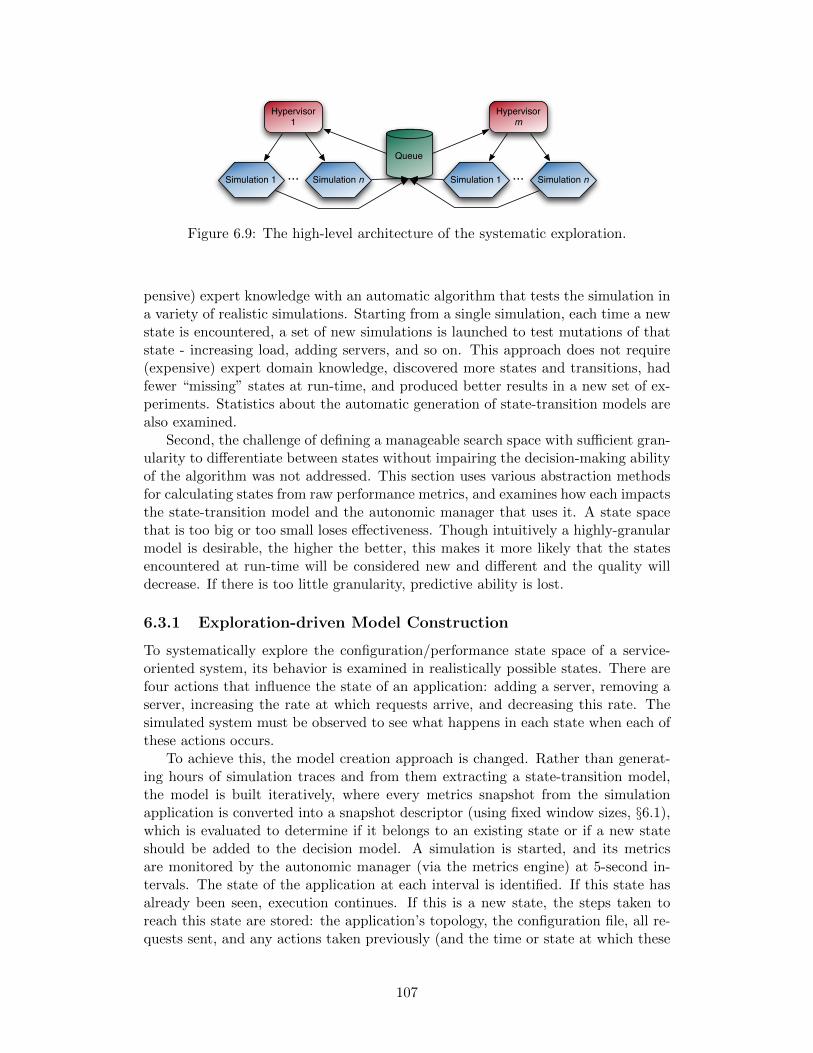
Hypervisor 1
Queue
Simulation 1 Simulation n...
Hypervisor m
Simulation 1 Simulation n...
Figure 6.9: The high-level architecture of the systematic exploration.
pensive) expert knowledge with an automatic algorithm that tests the simulation ina variety of realistic simulations. Starting from a single simulation, each time a newstate is encountered, a set of new simulations is launched to test mutations of thatstate - increasing load, adding servers, and so on. This approach does not require(expensive) expert domain knowledge, discovered more states and transitions, hadfewer “missing” states at run-time, and produced better results in a new set of ex-periments. Statistics about the automatic generation of state-transition models arealso examined.
Second, the challenge of defining a manageable search space with sufficient gran-ularity to differentiate between states without impairing the decision-making abilityof the algorithm was not addressed. This section uses various abstraction methodsfor calculating states from raw performance metrics, and examines how each impactsthe state-transition model and the autonomic manager that uses it. A state spacethat is too big or too small loses effectiveness. Though intuitively a highly-granularmodel is desirable, the higher the better, this makes it more likely that the statesencountered at run-time will be considered new and different and the quality willdecrease. If there is too little granularity, predictive ability is lost.
6.3.1 Exploration-driven Model Construction
To systematically explore the configuration/performance state space of a service-oriented system, its behavior is examined in realistically possible states. There arefour actions that influence the state of an application: adding a server, removing aserver, increasing the rate at which requests arrive, and decreasing this rate. Thesimulated system must be observed to see what happens in each state when each ofthese actions occurs.
To achieve this, the model creation approach is changed. Rather than generat-ing hours of simulation traces and from them extracting a state-transition model,the model is built iteratively, where every metrics snapshot from the simulationapplication is converted into a snapshot descriptor (using fixed window sizes, §6.1),which is evaluated to determine if it belongs to an existing state or if a new stateshould be added to the decision model. A simulation is started, and its metricsare monitored by the autonomic manager (via the metrics engine) at 5-second in-tervals. The state of the application at each interval is identified. If this state hasalready been seen, execution continues. If this is a new state, the steps taken toreach this state are stored: the application’s topology, the configuration file, all re-quests sent, and any actions taken previously (and the time or state at which these
107
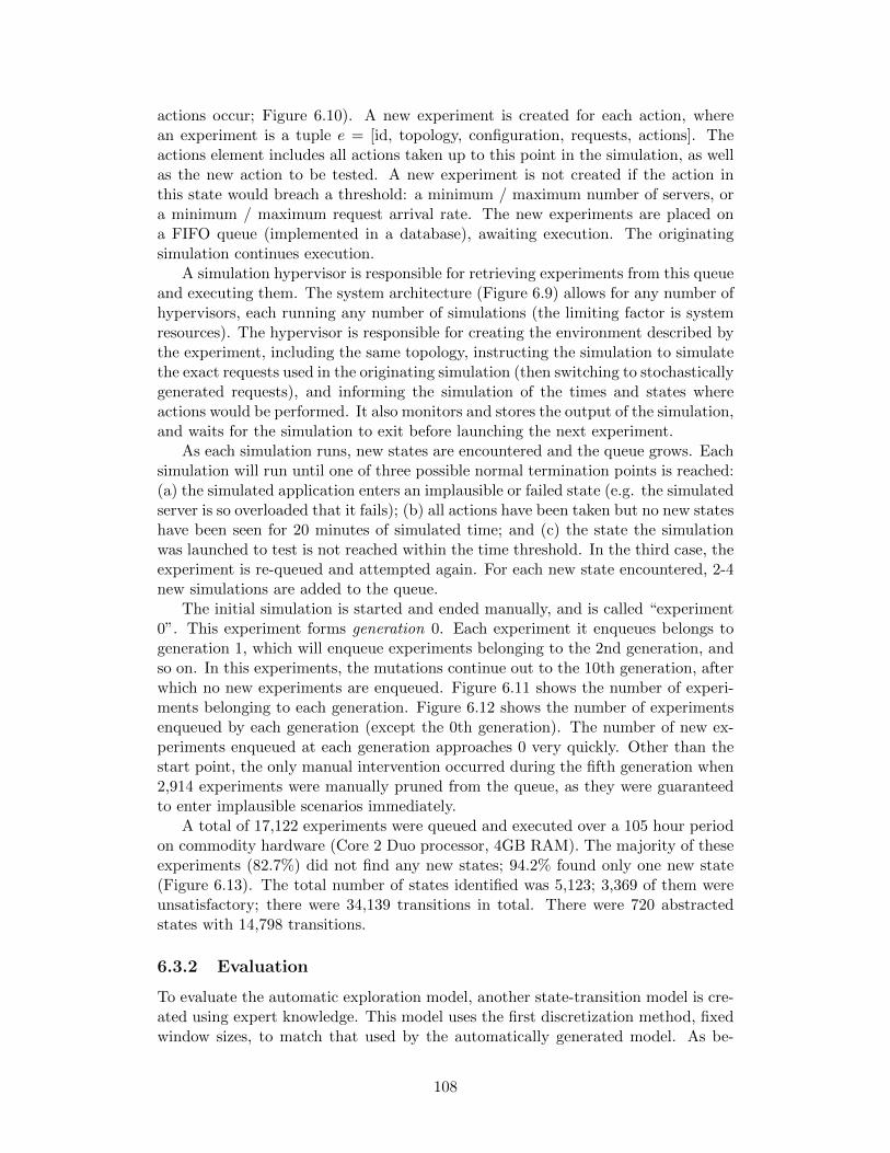
actions occur; Figure 6.10). A new experiment is created for each action, wherean experiment is a tuple e = [id, topology, configuration, requests, actions]. Theactions element includes all actions taken up to this point in the simulation, as wellas the new action to be tested. A new experiment is not created if the action inthis state would breach a threshold: a minimum / maximum number of servers, ora minimum / maximum request arrival rate. The new experiments are placed ona FIFO queue (implemented in a database), awaiting execution. The originatingsimulation continues execution.
A simulation hypervisor is responsible for retrieving experiments from this queueand executing them. The system architecture (Figure 6.9) allows for any number ofhypervisors, each running any number of simulations (the limiting factor is systemresources). The hypervisor is responsible for creating the environment described bythe experiment, including the same topology, instructing the simulation to simulatethe exact requests used in the originating simulation (then switching to stochasticallygenerated requests), and informing the simulation of the times and states whereactions would be performed. It also monitors and stores the output of the simulation,and waits for the simulation to exit before launching the next experiment.
As each simulation runs, new states are encountered and the queue grows. Eachsimulation will run until one of three possible normal termination points is reached:(a) the simulated application enters an implausible or failed state (e.g. the simulatedserver is so overloaded that it fails); (b) all actions have been taken but no new stateshave been seen for 20 minutes of simulated time; and (c) the state the simulationwas launched to test is not reached within the time threshold. In the third case, theexperiment is re-queued and attempted again. For each new state encountered, 2-4new simulations are added to the queue.
The initial simulation is started and ended manually, and is called “experiment0”. This experiment forms generation 0. Each experiment it enqueues belongs togeneration 1, which will enqueue experiments belonging to the 2nd generation, andso on. In this experiments, the mutations continue out to the 10th generation, afterwhich no new experiments are enqueued. Figure 6.11 shows the number of experi-ments belonging to each generation. Figure 6.12 shows the number of experimentsenqueued by each generation (except the 0th generation). The number of new ex-periments enqueued at each generation approaches 0 very quickly. Other than thestart point, the only manual intervention occurred during the fifth generation when2,914 experiments were manually pruned from the queue, as they were guaranteedto enter implausible scenarios immediately.
A total of 17,122 experiments were queued and executed over a 105 hour periodon commodity hardware (Core 2 Duo processor, 4GB RAM). The majority of theseexperiments (82.7%) did not find any new states; 94.2% found only one new state(Figure 6.13). The total number of states identified was 5,123; 3,369 of them wereunsatisfactory; there were 34,139 transitions in total. There were 720 abstractedstates with 14,798 transitions.
6.3.2 Evaluation
To evaluate the automatic exploration model, another state-transition model is cre-ated using expert knowledge. This model uses the first discretization method, fixedwindow sizes, to match that used by the automatically generated model. As be-
108
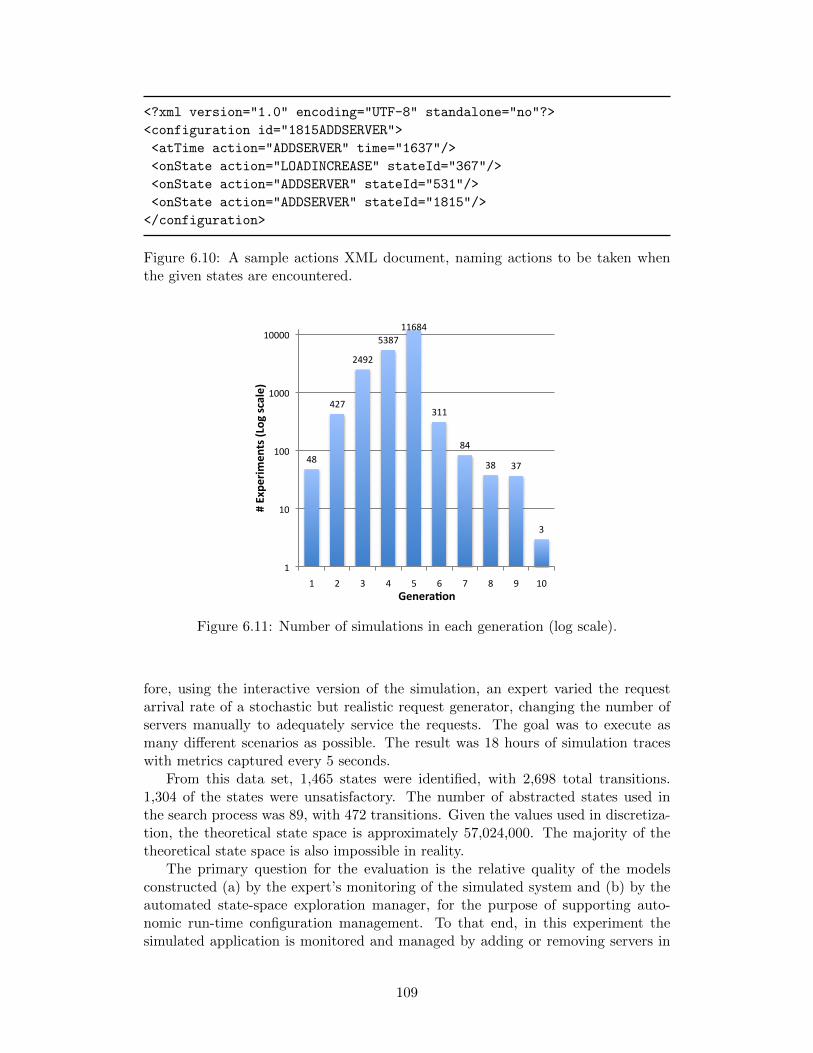
<?xml version="1.0" encoding="UTF-8" standalone="no"?>
<configuration id="1815ADDSERVER">
<atTime action="ADDSERVER" time="1637"/>
<onState action="LOADINCREASE" stateId="367"/>
<onState action="ADDSERVER" stateId="531"/>
<onState action="ADDSERVER" stateId="1815"/>
</configuration>
Figure 6.10: A sample actions XML document, naming actions to be taken whenthe given states are encountered.
48
427
2492
5387 11684
311
84
38 37
3
1
10
100
1000
10000
1 2 3 4 5 6 7 8 9 10
# Expe
rimen
ts (Log scale)
Genera6on
Figure 6.11: Number of simulations in each generation (log scale).
fore, using the interactive version of the simulation, an expert varied the requestarrival rate of a stochastic but realistic request generator, changing the number ofservers manually to adequately service the requests. The goal was to execute asmany different scenarios as possible. The result was 18 hours of simulation traceswith metrics captured every 5 seconds.
From this data set, 1,465 states were identified, with 2,698 total transitions.1,304 of the states were unsatisfactory. The number of abstracted states used inthe search process was 89, with 472 transitions. Given the values used in discretiza-tion, the theoretical state space is approximately 57,024,000. The majority of thetheoretical state space is also impossible in reality.
The primary question for the evaluation is the relative quality of the modelsconstructed (a) by the expert’s monitoring of the simulated system and (b) by theautomated state-space exploration manager, for the purpose of supporting auto-nomic run-time configuration management. To that end, in this experiment thesimulated application is monitored and managed by adding or removing servers in
109
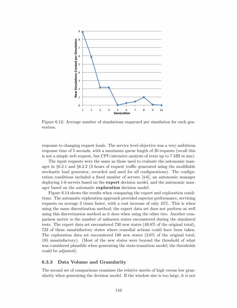
0
1
2
3
4
5
6
7
8
9
1 2 3 4 5 6 7 8 9 10
New
Sim
ula+
ons Created pe
r Simula+
on
Genera+on
Figure 6.12: Average number of simulations enqueued per simulation for each gen-eration.
response to changing request loads. The service level objective was a very ambitiousresponse time of 5 seconds, with a maximum queue length of 20 requests (recall thisis not a simple web request, but CPU-intensive analysis of texts up to 7 MB in size).
The input requests were the same as those used to evaluate the autonomic man-ager in §6.2.1 and §6.2.2 (3 hours of request traffic generated using the modifiablestochastic load generator, recorded and used for all configurations). The configu-ration conditions included a fixed number of servers [4-6], an autonomic managerdeploying 1-6 servers based on the expert decision model, and the autonomic man-ager based on the automatic exploration decision model.
Figure 6.14 shows the results when comparing the expert and exploration condi-tions. The automatic exploration approach provided superior performance, servicingrequests on average 3 times faster, with a cost increase of only 45%. This is whenusing the same discretization method; the expert data set does not perform as wellusing this discretization method as it does when using the other two. Another com-parison metric is the number of unknown states encountered during the simulatedtests. The expert data set encountered 730 new states (49.8% of the original total),723 of them unsatisfactory states where remedial actions could have been taken.The exploration data set encountered 188 new states (3.6% of the original total,185 unsatisfactory). (Most of the new states were beyond the threshold of whatwas considered plausible when generating the state-transition model; the thresholdscould be adjusted).
6.3.3 Data Volume and Granularity
The second set of comparisons examines the relative merits of high versus low gran-ularity when generating the decision model. If the window size is too large, it is not
110
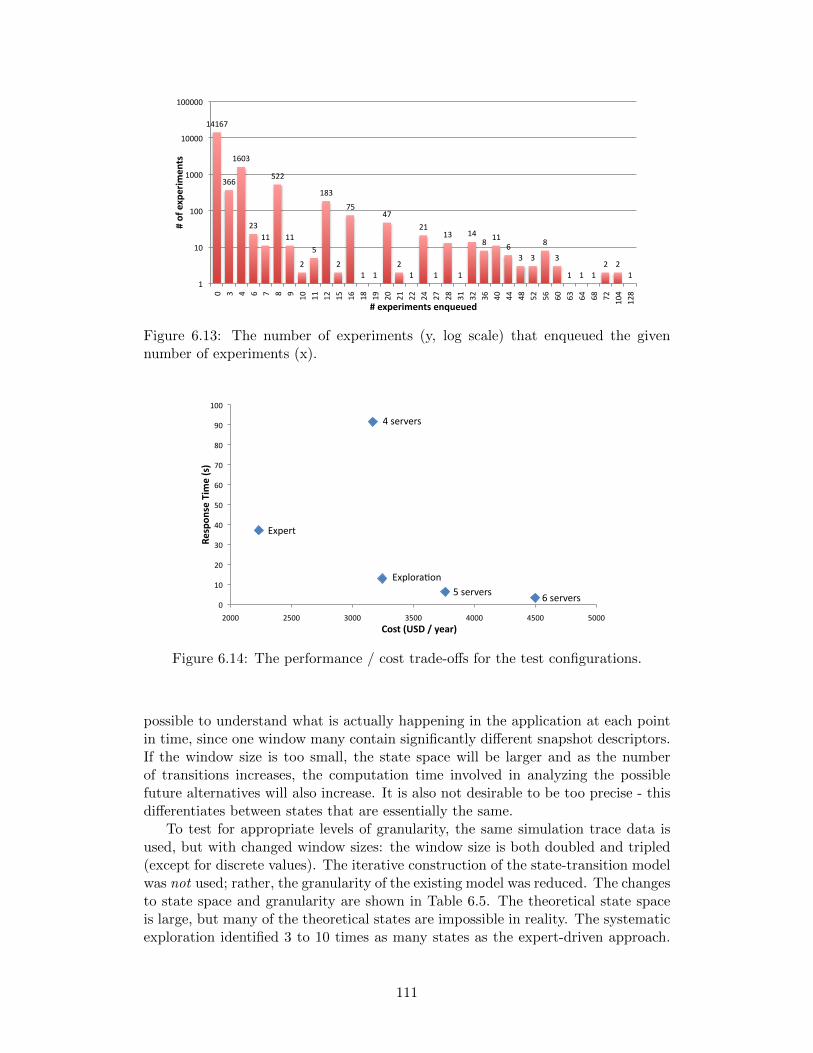
14167
366
1603
23 11
522
11
2
5
183
2
75
1 1
47
2 1
21
1
13
1
14 8
11 6
3 3
8
3
1 1 1 2 2
1 1
10
100
1000
10000
100000
0 3 4 6 7 8 9 10
11
12
15
16
18
19
20
21
22
24
27
28
31
32
36
40
44
48
52
56
60
63
64
68
72
104
128
# of experim
ents
# experiments enqueued
Figure 6.13: The number of experiments (y, log scale) that enqueued the givennumber of experiments (x).
4 servers
5 servers 6 servers
Expert
Explora0on
0
10
20
30
40
50
60
70
80
90
100
2000 2500 3000 3500 4000 4500 5000
Respon
se Tim
e (s)
Cost (USD / year)
Figure 6.14: The performance / cost trade-offs for the test configurations.
possible to understand what is actually happening in the application at each pointin time, since one window many contain significantly different snapshot descriptors.If the window size is too small, the state space will be larger and as the numberof transitions increases, the computation time involved in analyzing the possiblefuture alternatives will also increase. It is also not desirable to be too precise - thisdifferentiates between states that are essentially the same.
To test for appropriate levels of granularity, the same simulation trace data isused, but with changed window sizes: the window size is both doubled and tripled(except for discrete values). The iterative construction of the state-transition modelwas not used; rather, the granularity of the existing model was reduced. The changesto state space and granularity are shown in Table 6.5. The theoretical state spaceis large, but many of the theoretical states are impossible in reality. The systematicexploration identified 3 to 10 times as many states as the expert-driven approach.
111
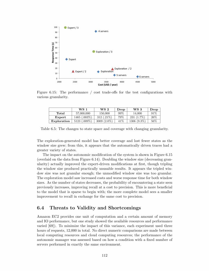
4 servers
5 servers 6 servers
Expert
Explora0on Expert / 2 Explora0on / 2
Expert / 3
Explora0on / 3
0
10
20
30
40
50
60
70
80
90
100
2000 2500 3000 3500 4000 4500 5000
Respon
se Tim
e (s)
Cost (USD / year)
Figure 6.15: The performance / cost trade-offs for the test configurations withvarious granularity.
WS 1 WS 2 Drop WS 3 Drop
Total 57,000,000 150,000 99% 14,000 91%
Expert 1465 (.003%) 312 (.21%) 79% 231 (1.7%) 26%
Exploration 5123 (.009%) 3009 (2.0%) 41% 1306 (9.3%) 56%
Table 6.5: The changes to state space and coverage with changing granularity.
The exploration-generated model has better coverage and lost fewer states as thewindow size grew; from this, it appears that the automatically driven traces had agreater variety of states.
The impact on the autonomic modification of the system is shown in Figure 6.15(overlaid on the data from Figure 6.14). Doubling the window size (decreasing gran-ularity) actually improved the expert-driven modifications at first, though triplingthe window size produced practically unusable results. It appears the tripled win-dow size was not granular enough; the unmodified window size was too granular.The exploration model saw increased costs and worse response time for both windowsizes. As the number of states decreases, the probability of encountering a state seenpreviously increases, improving recall at a cost to precision. This is more beneficialto the model that is sparse to begin with; the more complete model sees a smallerimprovement to recall in exchange for the same cost to precision.
6.4 Threats to Validity and Shortcomings
Amazon EC2 provides one unit of computation and a certain amount of memoryand IO performance, but one study showed the available resources and performancevaried [69]). To minimize the impact of this variance, each experiment used threehours of requests, 12,000 in total. No direct numeric comparisons are made betweenlocal computing resources and cloud computing resources; the performance of theautonomic manager was assessed based on how a condition with a fixed number ofservers performed in exactly the same environment.
112
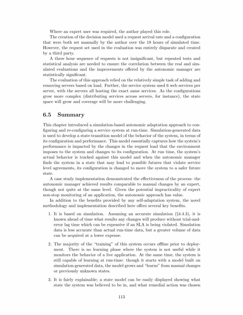
Where an expert user was required, the author played this role.The creation of the decision model used a request arrival rate and a configuration
that were both set manually by the author over the 18 hours of simulated time.However, the request set used in the evaluation was entirely disparate and createdby a third party.
A three hour sequence of requests is not insignificant, but repeated tests andstatistical analysis are needed to ensure the correlation between the real and sim-ulated evaluations and the improvements offered by the autonomic manager arestatistically significant.
The evaluation of this approach relied on the relatively simple task of adding andremoving servers based on load. Further, the service system used 6 web services perserver, with the servers all hosting the exact same services. As the configurationsgrow more complex (distributing services across servers, for instance), the statespace will grow and coverage will be more challenging.
6.5 Summary
This chapter introduced a simulation-based autonomic adaptation approach to con-figuring and re-configuring a service system at run-time. Simulation-generated datais used to develop a state-transition model of the behavior of the system, in terms ofits configuration and performance. This model essentially captures how the system’sperformance is impacted by the changes in the request load that the environmentimposes to the system and changes to its configuration. At run time, the system’sactual behavior is tracked against this model and when the autonomic managerfinds the system in a state that may lead to possible futures that violate servicelevel agreements, its configuration is changed to move the system to a safer futurestate.
A case study implementation demonstrated the effectiveness of the process: theautonomic manager achieved results comparable to manual changes by an expert,though not quite at the same level. Given the potential impracticality of expertnon-stop monitoring of an application, the autonomic approach has value.
In addition to the benefits provided by any self-adaptation system, the novelmethodology and implementation described here offers several key benefits.
1. It is based on simulation. Assuming an accurate simulation (§4.4.3), it isknown ahead of time what results any changes will produce without trial-and-error lag time which can be expensive if an SLA is being violated. Simulationdata is less accurate than actual run-time data, but a greater volume of datacan be acquired at a lower expense.
2. The majority of the “training” of this system occurs offline prior to deploy-ment. There is no learning phase where the system is not useful while itmonitors the behavior of a live application. At the same time, the system isstill capable of learning at run-time: though it starts with a model built onsimulation-generated data, the model grows and “learns” from manual changesor previously unknown states.
3. It is fairly explainable; a state model can be easily displayed showing whatstate the system was believed to be in, and what remedial action was chosen
113
as a result. Using the dashboard that is part of the simulation framework, asystem manager can review simulated “what if” scenarios. This understandingis intended to help resolve issues that administrators may have with allowingan application to make its own decisions.
4. It supports dynamic SLAs, in that, changing the service level agreement doesnot require re-learning the entire model; new SLAs can be accommodatedby a relatively inexpensive refresh of the state-transition model, where theclassification of the equivalence behavioral classes are updated to reflect theirconformance to the new SLA.
This set of contributions was further extended to replace the (expensive) expertuser with an automated system that recursively simulated various mutations ofeach state of a simulated application, creating a more complete decision model.This automatic creation of a decision model offers a low-cost solution for autonomicself-configuration, which in this case was able to achieve average results closer to adefined service level objective.
Finally, the challenge of creating a state-transition model that balances accu-racy, size of the state space, and the granularity of the discretization. Empiricalresults were presented on the growth of the state-transition model over the variousgenerations of the automatic creation. Trade-offs in granularity when discretizingraw performance metrics into states that meaningfully differentiate between actualapplication states were studied, finding that it is possible to be too vague and tobe too precise, and establishing empirically the appropriate balance for this ap-plication. Though the quality of the exploration-generated model deteriorated asgranularity decreased, the low cost of CPU time versus expensive expert knowledgegives automatic exploration an advantage.
114
Chapter 7
Conclusion and Future Work
Service-oriented systems offer useful and desirable features like loose-coupling, en-capsulation, network management, and enable interoperable multiple-entity serviceinteractions. The complexity introduced by these features can result in unsatisfy-ing interactions between service consumers and service providers: they are difficultfor providers to manage and difficult for consumers to specify, particularly non-functional requirements like performance.
This dissertation explored some of these challenges: the problems with currentapproaches to service level agreements, the motivation to involve the customer in anunderstandable process to increase their perceived value, the difficulty in asking con-sumers to perceive value without experience and in understanding how consumerstrade-off desired quality and trade-offs, and in general the benefits of understand-able, explainable, available information.
Simulation was examined as a promising solution. A set of proposed canonicalcharacteristics was defined and used to assess the existing state-of-the-art solutionsfor simulating service-oriented architectures. These solutions offered inadequatesupport for metrics gathering and visualizing, run-time interaction, emulation, ex-tensibility, and automatic generation: generally, they had insufficient inability toaccurately predict a performance-based predicted narrative for the behavior of aservice, and required substantial effort to produce. One primary research objectivewas to develop a framework, an approach, and a set of tools to support simulat-ing service-oriented systems with emphasis on metrics generation and minimizingdevelopment effort. A second objective was to employ this framework to produceworking, accurate simulations for real-world service systems, to demonstrate notonly the framework but also simulation-driven tools.
Existing approaches to configuration management do not make use of simula-tion to predict performance; instead, data from real-world deployed systems is useddirectly. This data is more expensive to produce, but is guaranteed to be accurate.When simulation is used, it is used to predict bottlenecks and resource contentionissues. Consumer-driven trade-off management is rarely considered. The problemswith SLAs and the potential of simulation to generate useful data to better informthe process of managing the lifecycle of an SLA led to the third objective, to use sim-ulation to manage an SLA throughout each phase of its lifecycle: (re-)negotiation,conversion to a configuration, and deployment.
One option for managing complex systems is self-management, or autonomic
115
computing. Existing approaches rely on real-world data, generated from a runningsystem that is not self-managed. This training phase is expensive. Autonomic workin services focuses on substituting services with other services that perform the samefunction, ignoring managing at the application level. Decisions made autonomicallymay be difficult for administrators to understand; decisions that can be explained arerare in existing systems. This motivated the fourth research objective, constructingan autonomic manager based on simulation-generated data, using an explainabledecision model, that re-configured the application and works in both simulation andin the real world.
The following section describes how each objective was achieved by describing aset of novel contributions in more detail.
7.1 Contributions Supporting Research Objectives
Objective: Demonstrate that authoring a simulation of a service-oriented systemneed not be prohibitively difficult, and that such simulations can produce a narrativethat offers useful and realistic information about the predicted performance of asoftware system.
A services-aware simulation framework (SASF) was introduced in Chapter 3.A systematic, comprehensive review of simulation frameworks for service-orientedsystems (using the proposed canonical characteristics) revealed shortcomings withexisting approaches. This contribution excels at producing a narrative of the pre-dicted performance of a service system based on past exemplars. It achieves thisby offering a powerful and extensible engine for collecting and visualizing metricsand the ability to generate a simulation from an existing standardized descriptionof the service, reducing development effort. Extensible libraries for common webservice functionality offer support better than (or at least comparable to) the stateof the art. The ability to replicate performance of service systems, and to test theservices using requests generated based on probabilistic models derived from realdata, improve the quality of the predicted narrative. Integration with real-worldcomponents allows for simplified validation in real situations. The unique abilityto systematically run large numbers of varied experiments simplifies generating vol-umes of performance data.
These key contributions are compared to the current state of the art in §2.3.7;SASF meets or exceeds the state of the art in all areas.
Objective: Use the simulation approach to produce simulated versions of real-worldservice systems using real performance data.
SASF was used to simulate Tivoli Provisioning Manager and the back-end servicefor the Text Analysis Portal for Research. The first demonstrates use of basic libraryfunctionality, the simulation engine, and the metrics engine. The second adds theuse of additional libraries, automated simulation generation, systematic simulationusing JIMMIE, and the Service Testing Module.
The use of the framework reduced development time and effort that would havebeen required otherwise. In the case of TPMsim, the framework is estimated tohave offered a 45% reduction in development effort. In the case of TAPoRsim, itsbehavior was replicated without manually authoring a single line of code. A set of
116
extensions was added, and still only 28% of the TAPoRsim code was hand-coded.TAPoRsim was statistically validated and shown to replicate response times with
millisecond accuracy with 95% confidence. Both simulations contribute valuabletest-beds to use for testing not only the specific application simulated, but alsogeneral simulation-driven methods and tools.
Objective: Show that simulation-driven tools can be used to help manage the gover-nance of software systems throughout the cycle of negotiating standards for serviceperformance, configuring the service to meet those standards, and evaluating andmonitoring ongoing compliance with those standards.
The first step in achieving this objective was contributing a new SLA lifecycle,one with a focus on re-evaluation and re-negotiation of the SLA as technical andbusiness needs change. Three additional contributions use simulation to assist eachphase of the lifecycle.
First, a methodology, tool, and numeric representation of trade-off balance andcost-benefit analysis to assist in understanding and choosing the balance amongdependent metrics. It was demonstrated that hundreds of candidate configurationscould be tested, visualized, and presented to a user who chose their preferred trade-offs. The tool narrowed down the candidate configurations by 94%.
Second, a question-answering methodology and tool that assists a service providerin producing a configuration that meets the SLA (through his or her interaction withthe tool), and in better understanding a service system generally. The approachwas demonstrated on two questions, on both the simulation and on a real-worlddeployment. A positive correlation between simulation-generated answers and thereal-world answers was observed. When asked to identify the best configurationfrom a set of hundreds of possible configurations, the answer produced by the ques-tion answering tool produced a configuration that performed better than the oneproposed by an expert with access to perfect information about the test scenario.
Finally, a monitoring and assessment tool that integrates simulated componentswith real-world services to use the flexible and powerful service testing modulesand the metrics/dashboard framework of SASF to produce, visualize, and storereal-world data. The tool was demonstrated exercising a real-world deployment ofTAPoR and visualizing simulation-generated metrics alongside real-world metrics.
Objective: Demonstrate that a decision model generated in simulation can be usedto reason about a real-world software system, to the point that such reasoning canbe trusted to re-configure the service at run-time.
A set of contributions centered on autonomically re-configuring a software systemat runtime achieves this objective. Simulation-generated data was used to contributea state-transition model of the behavior of the system, in terms of its configurationand performance. This model essentially captures how the system’s performance isimpacted by the changes in the request load that the environment imposes to thesystem and changes to its configuration. At run time, the system’s actual behavioris tracked against this model and when the autonomic manager finds the systemin a state that may lead to possible futures that violate service level agreements,its configuration is changed to move the system to a safer future state. Simulationallows for generating more data than might otherwise be available, all occurringoffline. The state-transition model can also be updated at run-time, both by adding
117
new states and by changing the SLA in response to business needs. This model canbe visualized and is explainable, addressing a need not usually met by autonomicsystems.
A case study implementation demonstrated the effectiveness of the process: theautonomic manager achieved results comparable to manual changes by an expert,though not quite at the same level. This was tested in both simulation and a real-world cloud computing environment. Given the potential impracticality of expertnon-stop monitoring of an application, this contribution has value.
To further this contribution, the decision model construction process was ex-tended to add an automated system that recursively simulated various mutationsof each state of a simulated application, creating a more complete decision model.This automatic creation of a decision model offers a low-cost solution for autonomicself-configuration, which in this case was able to achieve average results closer to adefined service level objective.
For the final contribution, the challenge of creating a state-transition model thatbalances accuracy, size of the state space, and the granularity of the discretizationwas addressed. Empirical results were presented on the growth of the state-transitionmodel over the various generations of the automatic creation. Trade-offs in granu-larity when discretizing raw performance metrics into states that meaningfully dif-ferentiate between actual application states were studied, finding that it is possibleto be too vague and to be too precise, and establishing empirically the appropriatebalance for this application.
7.2 Future Work
The SASF service testing module is useful for generating web service requests us-ing statistical distributions based on real-world information. However, in §4.2,this module proved insufficient to model more complex client behavior. Addinga StateMachineDrivenEndpoint to the SASF Simulation Engine libraries wouldallow simulation authors to define a state machine that governs the behavior ofan endpoint, and a set of messages that move it from one state to another. Thiswould further reduce simulation development time when more complex behavior isrequired.
Currently, SASF’s CPU-bound operation support is limited to performance pro-files for operations that are O(n) in time complexity, where n is the size of the input.Extending this support to more intensive operations, or modifying n to be anotherfactor, is a planned extension. The CPUServiceOperation library class will be ex-tended to offer a more flexible approach to instantiating a formula to calculate theprocessing time required for a request. This will better support simulation authorsand will make wsdl2sim available to more types of services.
Though simple composition of services is provided, more complex compositionsupport can be implemented by a simulated BPEL engine. This engine would readexisting BPEL documents and orchestrate a series of simulated messages to replicatethe behavior of a real-world BPEL engine. Though composition testing support isavailable in existing simulation frameworks, adding BPEL support to SASF wouldintegrate composition testing support with a framework capable of predicting anarrative and generating accurate performance metrics. Such a model would be
118
capable of supporting run-time composition.No one other than the author and those who helped implement the simulation
framework have used it to simulate applications; no user study of its usability forproducing simulated services has been conducted. The framework will be releasedas an open-source project; this would allow further assessment of its usefulness. Theframework could also be employed in a course project. This could identify additionalfeatures that would be useful to SASF.
Though TPMsim is shown to accurately replicate results from an emulation envi-ronment, no systematic approach using TPMsim to assist in configuring a real-worldTPM deployment is described. Future work includes recommending deploymentsgiven an input network topology. The approach would use JIMMIE to systemati-cally modify the number and location of content distribution depots, test how eachperforms when distributing files of varying sizes, and choose a configuration thatbest balances overall cost and total deployment time using the trade-off analysistool.
An emerging area of research is migrating existing software infrastructure tocloud-based infrastructures. These systems have different hardware profiles and dif-ferent cost-models, both of which are not always well understood. A future projectinvolves using simulation to predict both performance and cost in a leased com-puting environment (e.g., Amazon EC2). This migration question is believed to beapplication-specific, which makes an application-level simulation that can be auto-matically generated a useful tool for providing an answer. The current hardwareprofile of SASF is based on a non-virtualized machine. This profile would be modifiedto correspond to an Amazon compute unit, their defined unit of computation. Theprocess of constructing a performance profile would also change: IO performance isthe biggest differentiator between “real” and virtualized systems, so accurate rep-resentation of the predicted IO of a service is important. The first step in thiswork will be the migration of applications from physical computing environmentsto virtualized environments to better understand the differences.
The simulation-driven approaches to managing the SLA lifecycle have not beenvalidated in user studies that demonstrate that SLAs, configurations, and assess-ments are actually producing results that satisfy users. Though the methodologiesand tools meet the derived requirements (more co-created value, more informationsharing, analysis of trade-offs), and are shown to perform as designed, the last stepof a user study is a future project. The challenge of such a user study is asking indi-viduals to make decisions to maximize their perceived value in a service-managementscenario where they may have no intuitive sense of what is valuable. The study willtranslate this problem to a more common situation - instead of services processingrequests, the scenario might be cashiers processing customers in a retail environ-ment. Users will be asked to establish an SLA based on their intuition, then will beasked to use the trade-off analysis tool to choose SLA targets that maximize theirperceived value. The SLA target they specify will be simulated and the results willbe presented to them. Gap analysis will be used to measure their satisfaction withthe performance of the resulting configuration; the hypothesis is there will be lessof a gap between expectations and satisfaction when the trade-off analysis tool isused.
119
Bibliography
[1] E. Al-Masri and Q.H. Mahmoud. Qos-based discovery and ranking of webservices. In Computer Communications and Networks, 2007. ICCCN 2007.Proceedings of 16th International Conference on, pages 529 –534, 2007.
[2] H. Alla and R. David. Continuous and hybrid petri nets. Journal of CircuitsSystems Computers, 8(1):159–88, February 1998.
[3] D. Ardagna and B. Pernici. Adaptive service composition in flexible processes.Software Engineering, IEEE Transactions on, 33(6):369 –384, June 2007.
[4] Raphael M. Bahati, Michael A. Bauer, and Elvis M. Vieira. Adaptation strate-gies in policy-driven autonomic management. In ICAS ’07: Proceedings ofthe Third International Conference on Autonomic and Autonomous Systems,page 16, Washington, DC, USA, 2007. IEEE Computer Society.
[5] B.V. Balachandran, R. Balakrishnan, and K. Sivaramakrishnan. Capacity Plan-ning With Demand Uncertainty. The Engineering Economist, 43(1):49–72,1997.
[6] Jeanette Blomberg. Negotiating meaning of shared information in service sys-tem encounters. European Management Journal, 26(4):213 – 222, 2008.
[7] P. Brebner. Service-oriented performance modeling the mule enterprise ser-vice bus (esb) loan broker application. In Software Engineering and AdvancedApplications, 2009. SEAA ’09. 35th Euromicro Conference on, pages 404–411,2009.
[8] Paul Brebner, Liam O’Brien, and Jon Gray. Performance modeling for e-government service oriented architectures (SOAs). In Sonya Rosbotham Ash-ley Aitken, editor, ASWEC, pages 130–138, Australia, March 2008. ACS.
[9] Paul C. Brebner. Performance modeling for service oriented architectures. InICSE Companion ’08: Companion of the 30th international conference on Soft-ware engineering, pages 953–954, New York, NY, USA, 2008. ACM.
[10] P.F. Brown, R. Metz, and B.A. Hamilton. Reference model for service orientedarchitecture 1.0. OASIS Standard, 2006.
[11] Radu Calinescu and Marta Kwiatkowska. Using quantitative analysis to imple-ment autonomic IT systems. In ICSE ’09: Proceedings of the 2009 IEEE 31stInternational Conference on Software Engineering, pages 100–110, Washington,DC, USA, 2009. IEEE Computer Society.
120
[12] Valeria Cardellini, Emiliano Casalicchio, Vincenzo Grassi, Francesco Lo Presti,and Raffaela Mirandola. Qos-driven runtime adaptation of service oriented ar-chitectures. In Proceedings of the the 7th joint meeting of the European softwareengineering conference and the ACM SIGSOFT symposium on The foundationsof software engineering, ESEC/FSE ’09, pages 131–140, New York, NY, USA,2009. ACM.
[13] Jr. Cronin, J. Joseph and Steven A. Taylor. Measuring service quality: Areexamination and extension. The Journal of Marketing, 56(3):pp. 55–68, 1992.
[14] Jr. Cronin, J. Joseph and Steven A. Taylor. SERVPERF versus SERVQUAL:Reconciling performance-based and perceptions-minus-expectations measure-ment of service quality. The Journal of Marketing, 58(1):pp. 125–131, 1994.
[15] A. Dan, D. Davis, R. Kearney, A. Keller, R. King, D. Kuebler, H. Ludwig,M. Polan, M. Spreitzer, and A. Youssef. Web services on demand: Wsla-drivenautomated management. IBM Syst. J., 43:136–158, January 2004.
[16] R. David and H. Alla. Discrete, Continuous, and Hybrid Petri Nets. Springer,2010.
[17] D. Draheim, J. Grundy, J. Hosking, C. Lutteroth, and G. Weber. Realistic loadtesting of web applications. In Proceedings of the 10th European Conference onSoftware Maintenance and Reengineering, 2006. CSMR 2006., pages 56–67,March 2006.
[18] Panos Fitsilis. Practices and problems in managing electronic services usingSLAs. Information Management & Computer Security, 14(2):185–195, 2006.
[19] Forrester Research. Managing IT services from the outside in. http://www.
compuware.com/dl/ManagingITServicesFromTheOutsideIn.pdf.
[20] W3C Working Group. Web services glossary. http://www.w3.org/TR/
ws-gloss/.
[21] John Grundy, John Hosking, Lei Li, and Na Liu. Performance engineeringof service compositions. In SOSE ’06: Proceedings of the 2006 internationalworkshop on Service-oriented software engineering, pages 26–32, New York,NY, USA, 2006. ACM.
[22] Vasfi Gucer, Alfredo Olivieri, Ghufran Shah, Scott Berens, David Campbell,Fabrizio Salustri, Johan Raeymaeckers, Marc Remes, Murtuza Choilawala,Philippe Hamelin, and Ignacio Fernandez Gonzales. IBM redbook: Deploy-ment guide series: IBM Tivoli Provisioning Manager version 5.1, 2007.
[23] Nicole Hargrove, Ian Heritage, Prasad Imandi, Martin Keen, Wendy Neave,Laura Olson, Bhargav Perepa, and Andrew White. Service Lifecycle Gover-nance with IBM WebSphere Service Registry and Repository. IBM, December2009.
[24] P. Hasselmeyer, B. Koller, I. Kotsiopoulos, D. Kuo, and M. Parkin. NegotiatingSLAs with Dynamic Pricing Policies. Proceedings of the SOC@ Inside’07, 2007.
121
[25] Qiang He, Jun Yan, Ryszard Kowalczyk, Hai Jin, and Yun Yang. Lifetimeservice level agreement management with autonomous agents for services pro-vision. Information Sciences, 179(15):2591 – 2605, 2009. Including Special Issueon Computer-Supported Cooperative Work - Techniques and Applications, The11th Edition of the International Conference on CSCW in Design.
[26] IBM. An architectural blueprint for autonomic computing. Technical report,June 2006.
[27] IBM. Education assistant: Service quality manager client user function.http://publib.boulder.ibm.com/infocenter/ieduasst/tivv1r0/topic/
com.ibm.iea.netcoolsqm/netcoolsqm/4.1/provisioning/sqm_client_
user_function.pdf, January 2011.
[28] Gabriel Iszlai, Igor Fedorenko, and Mark Leitch. White paper: Large scaledeployment using Tivoli Provisioning Manager, 2008.
[29] Diane Jordan and John Evdemon. Web services business process executionlanguage version 2.0. OASIS Standard, 2007.
[30] Krishna Kant and Youjip Won. Server capacity planning for web traffic work-load. IEEE Transactions on Knowledge and Data Engineering, 11(5):731–747,1999.
[31] Alexander Keller and Heiko Ludwig. The wsla framework: Specifying andmonitoring service level agreements for web services. J. Netw. Syst. Manage.,11:57–81, March 2003.
[32] Jeffrey O. Kephart and David M. Chess. The vision of autonomic computing.Computer, 36(1):41–50, 2003.
[33] Sungung Kim, Hessam S. Sarjoughian, and Vignesh Elamvazhuthi. Devs-suite:a simulator supporting visual experimentation design and behavior monitoring.In SpringSim ’09: Proceedings of the 2009 Spring Simulation Multiconference,pages 1–7, San Diego, CA, USA, 2009. Society for Computer Simulation Inter-national.
[34] R.E. Korf. Depth-first iterative-deepening: An optimal admissible tree search.Artificial intelligence, 27(1):97–109, 1985.
[35] Giannis Koumoutsos, Spyros Denazis, and Kleanthis Thramboulidis. Sla e-negotiations, enforcement and management in an autonomic environment. InProceedings of the 3rd IEEE international workshop on Modelling AutonomicCommunications Environments, MACE ’08, pages 120–125, Berlin, Heidelberg,2008. Springer-Verlag.
[36] E.J. Langer. Rethinking the role of thought in social interaction. New directionsin attribution research, 2:35–58, 1978.
[37] Mark Leitch, Clement Au, Andrew Kaye-Cheveldayoff, and Cindy Lee. Whitepaper: IBM Tivoli Provisioning Manager 5.1 performance and scalability re-sults, 2007.
122

[38] T. Levitt. Production-line approach to service. Harvard Business Review,50(5):41—52, 1972.
[39] Marin Litoiu, Mircea Mihaescu, Dan Ionescu, and Bogdan Solomon. Scalableadaptive web services. In Proceedings of the 2nd international workshop onSystems development in SOA environments, SDSOA ’08, pages 47–52, NewYork, NY, USA, 2008. ACM.
[40] Marin Litoiu, Murray Woodside, and Tao Zheng. Hierarchical model-basedautonomic control of software systems. SIGSOFT Softw. Eng. Notes, 30:1–7,May 2005.
[41] Na Liu, John Grundy, and John Hosking. A visual language and environmentfor composing web services. In ASE ’05: Proceedings of the 20th IEEE/ACMinternational Conference on Automated software engineering, pages 321–324,New York, NY, USA, 2005. ACM.
[42] Yoke-Hean Low, Chu-Cheow Lim, Wentong Cai, Shell-Ying Huang, Wen-JingHsu, Sanjay Jain, and Stephen J. Turner. Survey of languages and runtimelibraries for parallel discrete-event simulation. SIMULATION, 72(3):170–186,1999.
[43] Richard Lutz. Quality is as quality does: An attitudinal perspective on con-sumer quality judgments. Presentation to the Marketing Science InstituteTrustees’ Meeting, Cambridge, MA, 1986.
[44] Khaled Mahbub and George Spanoudakis. Proactive sla negotiation for servicebased systems. In Proceedings of the 2010 6th World Congress on Services,SERVICES ’10, pages 519–526, Washington, DC, USA, 2010. IEEE ComputerSociety.
[45] E. Mancini, U. Villano, M. Rak, and R. Torella. A simulation-based frame-work for autonomic web services. In Parallel and Distributed Systems, 2005.Proceedings. 11th International Conference on, volume 2, pages 433 –437, 2005.
[46] D.A. Menasce and V. Almeida. Capacity Planning for Web Services: metrics,models, and methods. Prentice Hall PTR Upper Saddle River, NJ, USA, 2001.
[47] Peter K. Mills and Dennis J. Moberg. Perspectives on the technology of serviceoperations. The Academy of Management Review, 7(3):467–478, 1982.
[48] Richard Murch. Autonomic Computing. IBM Press, 2004.
[49] Richard E. Nance. Simulation programming languages: an abridged history.In Proceedings of the 27th conference on Winter simulation, WSC ’95, pages1307–1313, Washington, DC, USA, 1995. IEEE Computer Society.
[50] Srini Narayanan and Sheila A. McIlraith. Simulation, verification and auto-mated composition of web services. In WWW ’02: Proceedings of the 11thinternational conference on World Wide Web, pages 77–88, New York, NY,USA, 2002. ACM.
123
[51] Srini Narayanan and Sheila A. McIlraith. Simulation, verification and auto-mated composition of web services. In WWW ’02: Proceedings of the 11thinternational conference on World Wide Web, pages 77–88, New York, NY,USA, 2002. ACM.
[52] Srinivas Narayanan. Reasoning about actions in narrative understanding. InIJCAI’99: Proceedings of the 16th international joint conference on Artificalintelligence, pages 350–355, San Francisco, CA, USA, 1999. Morgan KaufmannPublishers Inc.
[53] Lars Nilsson, Michael D. Johnson, and Anders Gustafsson. The impact ofquality practices on customer satisfaction and business results: product versusservice organizations. Journal of Quality Management, 6(1):5 – 27, 2001.
[54] E. Di Nitto, C. Ghezzi, A. Metzger, M. Papazoglou, and K. Pohl. A journey tohighly dynamic, self-adaptive service-based applications. Automated SoftwareEngineering, 2008.
[55] Ramon Nou, Samuel Kounev, Ferran Juliı, and Jordi Torres. Autonomic qoscontrol in enterprise grid environments using online simulation. J. Syst. Softw.,82:486–502, March 2009.
[56] Manish Parashar. Autonomic Computing: Concepts, Infrastructure, and Ap-plications / Editor(s): Manish Parashar and Salim Hariri. Taylor & Francis,Inc., Bristol, PA, USA, 2007.
[57] A. Parasuraman, L.L. Berry, and V.A. Zeithaml. Refinement and reassessmentof the SERVQUAL scale. Journal of Retailing, 1991.
[58] A. Parasuraman, V.A. Zeithaml, and L.L. Berry. A conceptual model of servicequality and its implications for future research. The Journal of Marketing,49(4):41–50, 1985.
[59] A. Parasuraman, V.A. Zeithaml, and L.L. Berry. SERVQUAL: A Multiple-ItemScale For Measuring Consumer Perception. Journal of Retailing, 64(1):12–40,1988.
[60] A. Parasuraman, V.A. Zeithaml, and L.L. Berry. Reassessment of expectationsas a comparison standard in measuring service quality: implications for furtherresearch. The Journal of Marketing, 58(1):111–124, 1994.
[61] Lissa F. Pollacia. A survey of discrete event simulation and state-of-the-artdiscrete event languages. SIGSIM Simul. Dig., 20:8–25, September 1989.
[62] Franco Raimondi, James Skene, and Wolfgang Emmerich. Efficient online mon-itoring of web-service slas. In Proceedings of the 16th ACM SIGSOFT Interna-tional Symposium on Foundations of software engineering, SIGSOFT ’08/FSE-16, pages 170–180, New York, NY, USA, 2008. ACM.
[63] Geoffrey Rockwell. Tapor: Building a portal for text analysis. In RaymondSiemens and David Moorman, editors, Mind Technologies; Humanities Com-puting and the Canadian Academic Community, pages 285–299. University ofCalgary Press, Calgary, AB, 2006.
124
[64] Pablo Rossi and Zahir Tari. Software adaptation for service-oriented systems.In MW4SOC ’06: Proceedings of the 1st workshop on Middleware for ServiceOriented Computing (MW4SOC 2006), pages 12–17, New York, NY, USA,2006. ACM.
[65] Pawel Rubach and Michael Sobolewski. Dynamic sla negotiation in autonomicfederated environments. In Proceedings of the Confederated International Work-shops and Posters on On the Move to Meaningful Internet Systems: ADI,CAMS, EI2N, ISDE, IWSSA, MONET, OnToContent, ODIS, ORM, OTMAcademy, SWWS, SEMELS, Beyond SAWSDL, and COMBEK 2009, OTM’09, pages 248–258, Berlin, Heidelberg, 2009. Springer-Verlag.
[66] H S Sarjoughian and B Zeigler. DEVSJAVA: Basis for a DEVS-based collab-orative M&S environment. In Proceedings of the International Conference onWeb-Based Modeling and Simulation, pages 29–36, 1998.
[67] Hessam Sarjoughian, Sungung Kim, Muthukumar Ramaswamy, and StephenYau. A simulation framework for service-oriented computing systems. In WSC’08: Proceedings of the 40th Conference on Winter Simulation, pages 845–853.Winter Simulation Conference, 2008.
[68] A.G. Sawyer and P. Dickson. Psychological perspectives on consumer responseto sales promotion. Research on Sales Promotion: Collected Papers, MarketingScience Institute, Cambridge, MA, pages 1–21, 1984.
[69] Jorg Schad, Jens Dittrich, and Jorge-Arnulfo Quiane-Ruiz. Runtime measure-ments in the cloud: observing, analyzing, and reducing variance. Proc. VLDBEndow., 3:460–471, September 2010.
[70] Chungman Seo and Bernard P. Zeigler. Automating the devs modeling andsimulation interface to web services. In SpringSim ’09: Proceedings of the2009 Spring Simulation Multiconference, pages 1–8, San Diego, CA, USA, 2009.Society for Computer Simulation International.
[71] Michael Smit, Andrew Nisbet, Eleni Stroulia, Andrew Edgar, Gabriel Iszlai,and Marin Litoiu. Capacity planning for service-oriented architectures. InCASCON ’08: Proceedings of the 2008 conference of the Center for AdvancedStudies on collaborative research, pages 144–156, New York, NY, USA, 2008.ACM.
[72] Abhishek Srivastava and Paul G. Sorenson. Service selection based on cus-tomer rating of quality of service attributes. Web Services, IEEE InternationalConference on, 0:1–8, 2010.
[73] A Sulistio, C Yeo, and R Buyya. A taxonomy of computer-based simulationsand its mapping to parallel and distributed systems simulation tools. Software-Practice and Experience, Jan 2004.
[74] James J. Swain. Simulation software survey: To boldly go. OR/MS Today,36(5), October 2009.
125
[75] W Tsai, Chun Fan, Yinong Chen, and R Paul. DDSOS: a dynamic distributedservice-oriented simulation framework. Simulation Symposium, 2006. 39th An-nual, 2006.
[76] W.T. Tsai, Zhibin Cao, Xiao Wei, Ray Paul, Qian Huang, and Xin Sun. Mod-eling and simulation in service-oriented software development. Simulation,83(1):7–32, 2007.
[77] WT Tsai, R.A. Paul, B. Xiao, Z. Cao, and Y. Chen. PSML-S: A processspecification and modeling language for service oriented computing. In The9th IASTED international conference on software engineering and applications(SEA), Phoenix, pages 160–167, 2005.
[78] Stephen L. Vargo and Robert F. Lusch. The four service marketing myths.Journal of Service Research, 6(4):324–335, 2004.
[79] K. Verma, P. Doshi, K. Gomadam, J. Miller, and A. Sheth. Optimal adaptationin web processes with coordination constraints. In Web Services, 2006. ICWS’06. International Conference on, pages 257 –264, September 2006.
[80] Bernard Zeigler. Theory of Modeling and Simulation. Wiley Interscience, NewYork, 1st edition, 1976.
[81] Bernard Zeigler. Hierarchical, modular discrete-event modelling inan object-oriented environment. Simulation, 49(5):219–230, Nov 1987.10.1177/003754978704900506.
[82] V.A. Zeithaml. Consumer perceptions of price, quality, and value: a means-endmodel and synthesis of evidence. The Journal of Marketing, 52(3):2–22, 1988.
[83] V.A. Zeithaml, A. Parasuraman, and L.L. Berry. Delivering quality service:Balancing customer perceptions and expectations. Free Pr, 1990.
[84] Qi Zhang, Ludmila Cherkasova, Guy Mathews, Wayne Greene, and EvgeniaSmirni. R-capriccio: a capacity planning and anomaly detection tool forenterprise services with live workloads. In Middleware ’07: Proceedings ofthe ACM/IFIP/USENIX 2007 International Conference on Middleware, pages244–265, New York, NY, USA, 2007. Springer-Verlag New York, Inc.
[85] Farhana Zulkernine, Patrick Martin, Chris Craddock, and Kirk Wilson. Apolicy-based middleware for web services sla negotiation. In Proceedings ofthe 2009 IEEE International Conference on Web Services, ICWS ’09, pages1043–1050, Washington, DC, USA, 2009. IEEE Computer Society.
126


![[image] - Animorphs Forumanimorphsforum.com/uploads/files/arpitnathany/K A Applegate... · It was ninety-nine-point-nine-percent successful. It had stopped his heart, his kidneys,](https://img.pdfslide.us/doc/110x75/5aed6c247f8b9a3b2e908fc0/image-animorphs-a-applegateit-was-ninety-nine-point-nine-percent-successful.jpg)


![The Ninety Nine Diseases of Pressure Equipment[1]](https://img.pdfslide.us/doc/110x75/55cf994a550346d0339c9bce/the-ninety-nine-diseases-of-pressure-equipment1.jpg)
