Embed Size (px)
Citation preview
GRIP
New Technologies for DSM to Support
Traditional Soil Survey
M.C. Nolin, I. Perron, M.A. Niang,
M. Bernier et X. Geng
2012 CLRN Workshop, Lac Beauport Sunday, June, 3rd 2012
10MOA01001
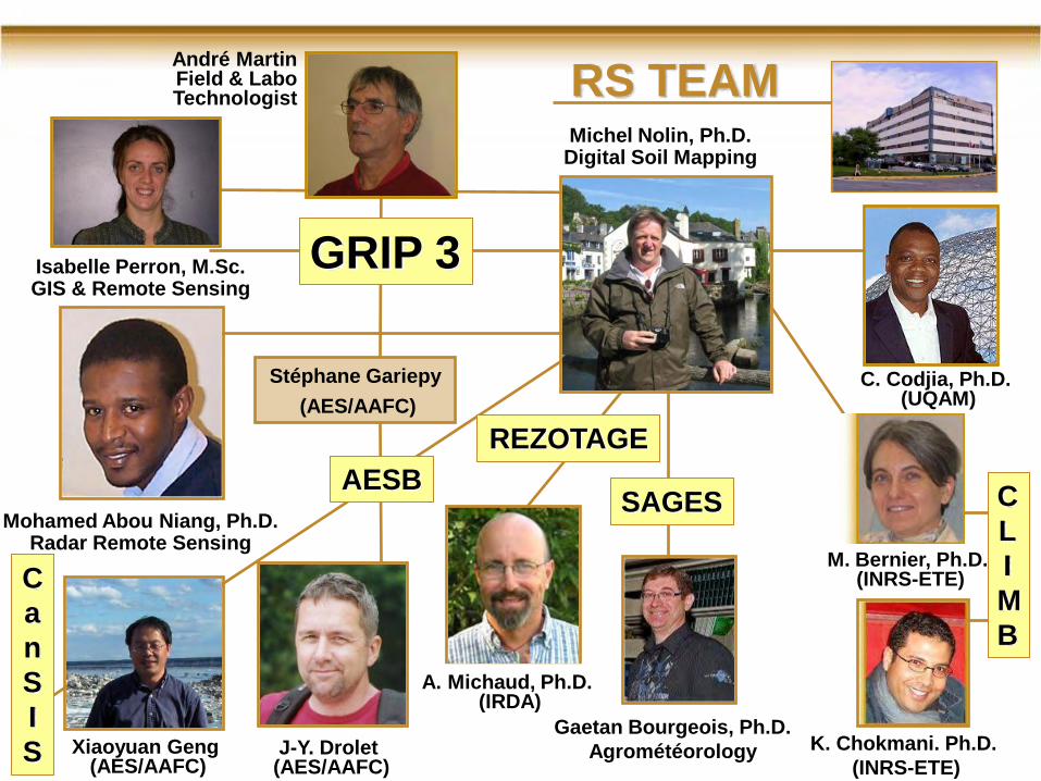
André Martin Field & Labo Technologist
M. Bernier, Ph.D. (INRS-ETE)
K. Chokmani. Ph.D.
(INRS-ETE)
C. Codjia, Ph.D. (UQAM)
Michel Nolin, Ph.D. Digital Soil Mapping
Gaetan Bourgeois, Ph.D.
Agrométéorology
SAGES
GRIP 3
Mohamed Abou Niang, Ph.D. Radar Remote Sensing
Isabelle Perron, M.Sc. GIS & Remote Sensing
C
L
I
M
B
RS TEAM
A. Michaud, Ph.D. (IRDA)
Xiaoyuan Geng (AES/AAFC)
REZOTAGE
AESB
J-Y. Drolet (AES/AAFC)
Stéphane Gariepy
(AES/AAFC)
C
a
n
S
I
S
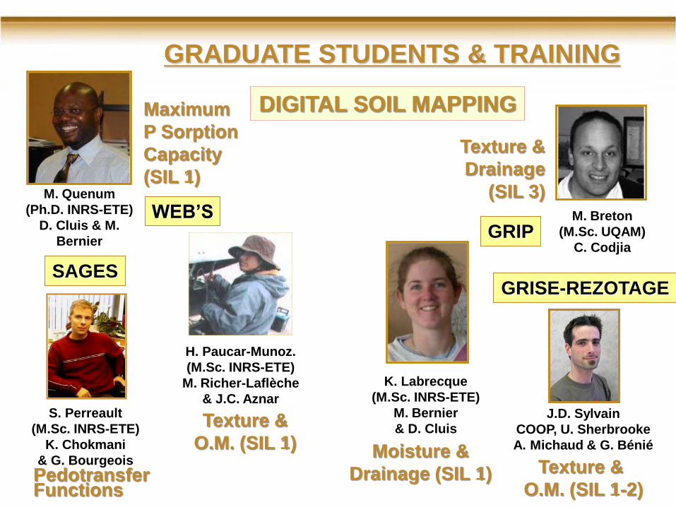
GRADUATE STUDENTS & TRAINING
SAGES
S. Perreault
(M.Sc. INRS-ETE)
K. Chokmani
& G. Bourgeois
J.D. Sylvain
COOP, U. Sherbrooke
A. Michaud & G. Bénié
K. Labrecque
(M.Sc. INRS-ETE)
M. Bernier
& D. Cluis
M. Quenum
(Ph.D. INRS-ETE)
D. Cluis & M.
Bernier
H. Paucar-Munoz.
(M.Sc. INRS-ETE)
M. Richer-Laflèche
& J.C. Aznar
M. Breton
(M.Sc. UQAM)
C. Codjia GRIP
WEB’S
Pedotransfer Functions
DIGITAL SOIL MAPPING Maximum
P Sorption
Capacity
(SIL 1)
Texture &
Drainage
(SIL 3)
Moisture &
Drainage (SIL 1)
Texture &
O.M. (SIL 1)
Texture &
O.M. (SIL 1-2)
GRISE-REZOTAGE
4
Outline
• State of Soil Mapping in Quebec
• Digital Soil Mapping
• Ancillary variables and Tools
• Scale-Based Results (SIL)
– Soil Drainage Classes
– Surface Soil Texture Groups
– Sand, Silt, Clay & O.M. Contents
• Conclusions Luc Lamontagne
5
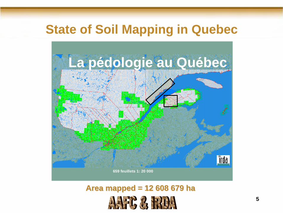
State of Soil Mapping in Quebec
27
27
56
TERREBONNE
ARGENTEUIL
DEUX-MONTAGNES
VAUDREUIL
SOULANGES
HUNTINGTON
BEAUHARNOIS
BROME
MISSISQUOI
SHEFFORD
RICHMOND
SHERBROO KE
COMPTON
STANSTEAD
CHATEAUGUAY
NAPIERVILLE
LAPRAIRIE
CHAMBLY
ROUVILLE
IBERVILLLE
ST-JEAN
VERCHÈRES
ST-HYACI NTHEBAGOT
RICHELIEU
DRUMMOND
FRONTENAC
BEAUCE
LOTBINIÈRE
MÉGANTI C
ARTHABASKA
NICOLET
YAMASKA
DORCHESTER
LÉVISBELLECHASSE
MONTMAGNY
L'ISLET
Ïle -a ux -Co udres
Île d 'o rléans
Ïl e-aux-G rues
KAMOURASKA
RIVIÈRE-DU-LOUP
TÉMISCOUATA
RIMOUSK I
MATANE
MATAPÉDIA
GASPÉ-OUEST
BONAVENTURE
GASPÉ-EST
CHARLEVOIX-EST
CHI CO UTIMI
LAC ST-JEAN-EST
LAC ST-JEAN-OUEST
MONTMORENCY(Cô te-de-Bea upré)
QUÉBEC
PORTNEUF
Champlain-Lav io le tte
ST-MAURICE
MASKI NO NG É
BERTHIER
JOLIETTE
MONTCALM
L'ASSOMPTION
HULL
PAPINEAU
LABELLE
GATINEAU
PONTIAC
TÉMISCAMINGUE
ABITIBI
WOLFE
CHARLEVOIX-OUEST
Sai nt -Roch- de- Richelieu
Fleu
ve S
aint-L
auren
t
Ba ie-d es- Chale urs
Ile d 'A n ti co sti
Rivi è
r e d e
s Pr a
ir ies
Rivièr
e Bati s
can
659 feuillets 1: 20 000
La pédologie au Québec
Area mapped = 12 608 679 ha
6
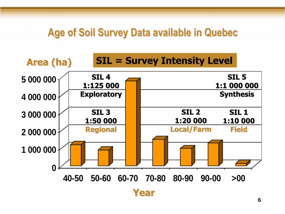
0
1 000 000
2 000 000
3 000 000
4 000 000
5 000 000
40-50 50-60 60-70 70-80 80-90 90-00 >00
Area (ha)
Year
Age of Soil Survey Data available in Quebec
SIL 2 1:20 000
Local/Farm
SIL 1 1:10 000
Field
SIL 3 1:50 000 Regional
SIL = Survey Intensity Level
SIL 5 1:1 000 000
Synthesis
SIL 4 1:125 000
Exploratory
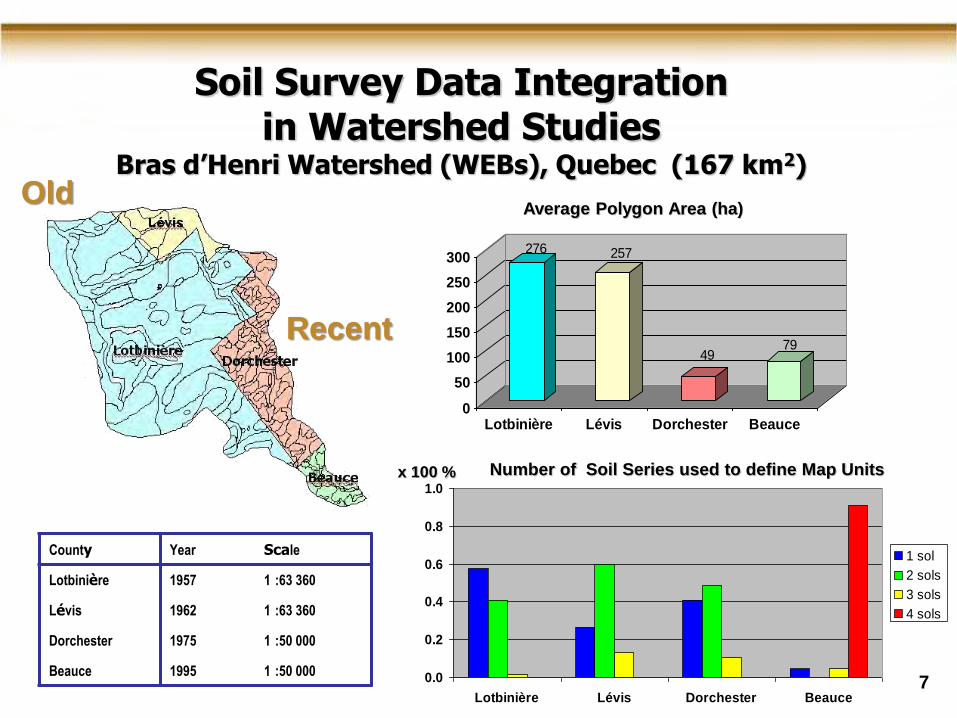
276 257
4979
0
50
100
150
200
250
300
Lotbinière Lévis Dorchester Beauce
Superficie moyenne des polygones (ha)
0.0
0.2
0.4
0.6
0.8
1.0
Lotbinière Lévis Dorchester Beauce
1 sol
2 sols
3 sols
4 sols
County Year Scale
Lotbinière 1957 1 :63 360
Lévis 1962 1 :63 360
Dorchester 1975 1 :50 000
Beauce 1995 1 :50 000
Soil Survey Data Integration in Watershed Studies
Bras d’Henri Watershed (WEBs), Quebec (167 km2)
Number of Soil Series used to define Map Units
Average Polygon Area (ha)
x 100 %
7
Old
Recent
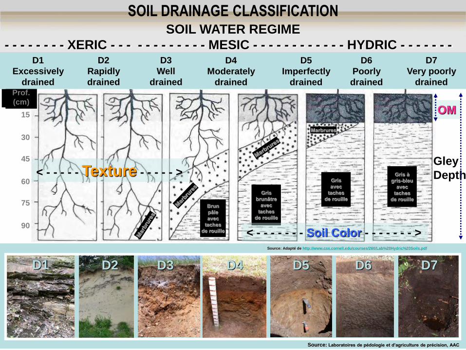
SOIL DRAINAGE CLASSIFICATION SOIL WATER REGIME
- - - - - - - - XERIC - - - - - - - - - - - - MESIC - - - - - - - - - - - - HYDRIC - - - - - - -
30
60
90
15
45
75
Prof.
(cm)
Brun
pâle
avec
taches
de rouille
Gris
brunâtre
avec
taches
de rouille
Gris
avec
taches
de rouille
Gris à
gris-bleu
avec
taches
de rouille
Marbrures
OM
Gley
Depth
< - - - - - - - Soil Color - - - - - - - >
< - - - - - Texture - - - - - >
Source: Laboratoires de pédologie et d’agriculture de précision, AAC
D1 D3 D4 D5 D6 D7 D2
Source: Adapté de http://www.css.cornell.edu/courses/260/Lab%20Hydric%20Soils.pdf
D1
Excessively
drained
D4
Moderately
drained
D5
Imperfectly
drained
D6
Poorly
drained
D7
Very poorly
drained
D3
Well
drained
D2
Rapidly
drained
9
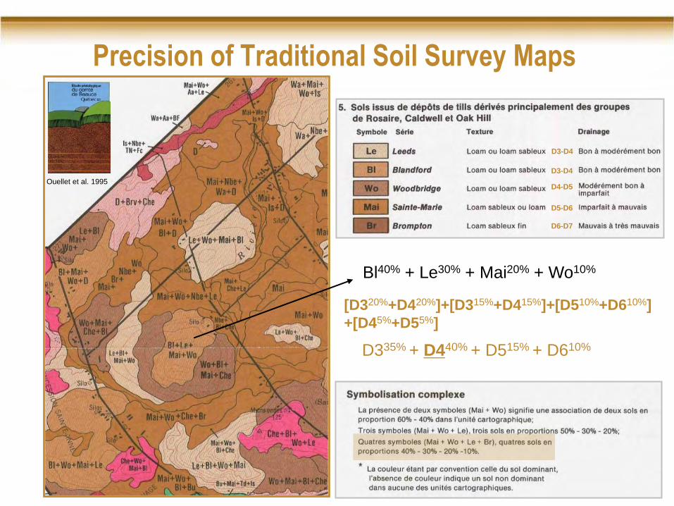
Precision of Traditional Soil Survey Maps
Bl40% + Le30% + Mai20% + Wo10%
D3-D4
D3-D4
D4-D5
D5-D6
D6-D7
[D320%+D420%]+[D315%+D415%]+[D510%+D610%]
+[D45%+D55%]
D335% + D440% + D515% + D610%
Ouellet et al. 1995
10
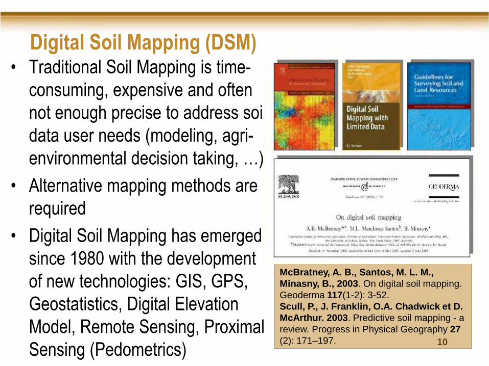
Digital Soil Mapping (DSM) • Traditional Soil Mapping is time-
consuming, expensive and often
not enough precise to address soil
data user needs (modeling, agri-
environmental decision taking, …)
• Alternative mapping methods are
required
• Digital Soil Mapping has emerged
since 1980 with the development
of new technologies: GIS, GPS,
Geostatistics, Digital Elevation
Model, Remote Sensing, Proximal
Sensing (Pedometrics)
McBratney, A. B., Santos, M. L. M.,
Minasny, B., 2003. On digital soil mapping.
Geoderma 117(1-2): 3-52.
Scull, P., J. Franklin, O.A. Chadwick et D.
McArthur. 2003. Predictive soil mapping - a
review. Progress in Physical Geography 27
(2): 171–197.
12
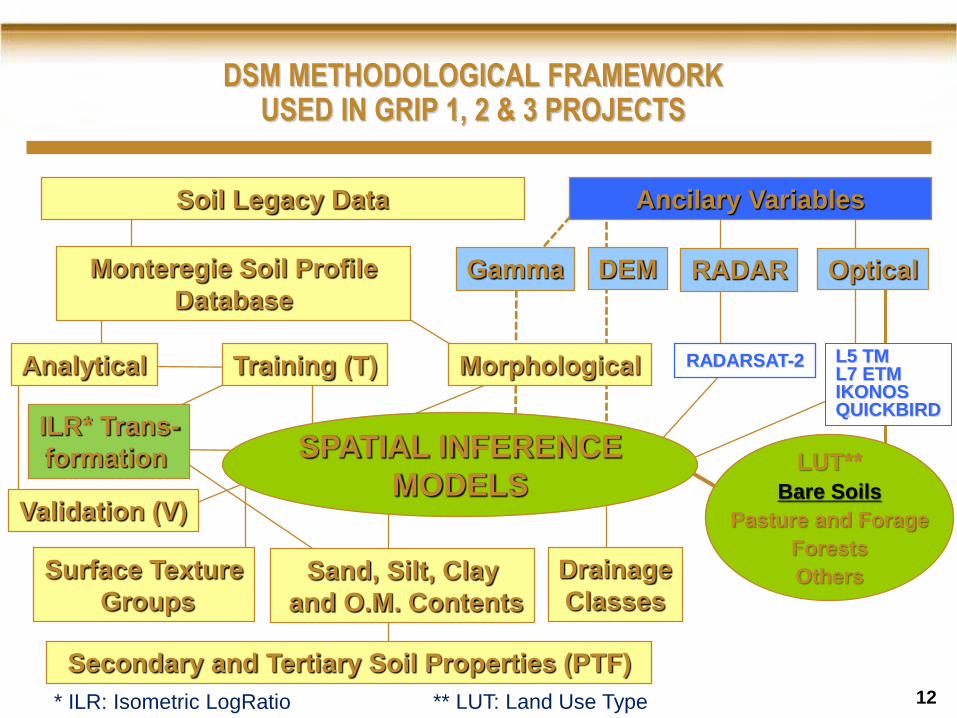
DSM METHODOLOGICAL FRAMEWORK USED IN GRIP 1, 2 & 3 PROJECTS
Soil Legacy Data
RADARSAT-2
Ancilary Variables
RADAR
Sand, Silt, Clay
and O.M. Contents
Secondary and Tertiary Soil Properties (PTF)
LUT**
Bare Soils
Pasture and Forage
Forests
Others
SPATIAL INFERENCE
MODELS Validation (V)
Analytical Morphological Training (T)
Monteregie Soil Profile
Database Optical
L5 TM L7 ETM IKONOS QUICKBIRD
Surface Texture
Groups
Gamma DEM
** LUT: Land Use Type
Drainage
Classes
ILR* Trans-
formation
* ILR: Isometric LogRatio
13
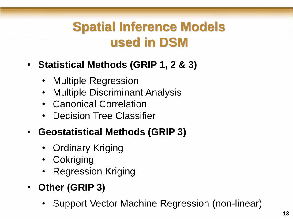
Spatial Inference Models
used in DSM
• Statistical Methods (GRIP 1, 2 & 3)
• Multiple Regression
• Multiple Discriminant Analysis
• Canonical Correlation
• Decision Tree Classifier
• Geostatistical Methods (GRIP 3)
• Ordinary Kriging
• Cokriging
• Regression Kriging
• Other (GRIP 3)
• Support Vector Machine Regression (non-linear)
14
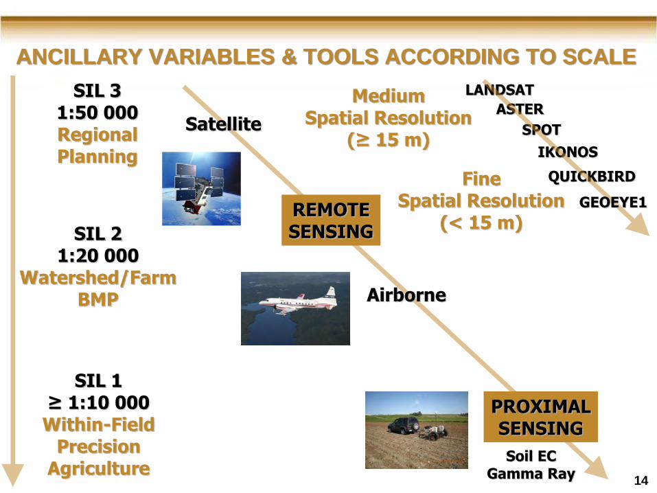
ANCILLARY VARIABLES & TOOLS ACCORDING TO SCALE
SIL 2 1:20 000
Watershed/Farm BMP
SIL 1 ≥ 1:10 000 Within-Field
Precision Agriculture
SIL 3 1:50 000 Regional Planning
REMOTE SENSING
PROXIMAL SENSING
Satellite
Airborne
Medium Spatial Resolution
(≥ 15 m)
Fine Spatial Resolution
(< 15 m)
LANDSAT
ASTER
SPOT
IKONOS
QUICKBIRD
Soil EC Gamma Ray
GEOEYE1
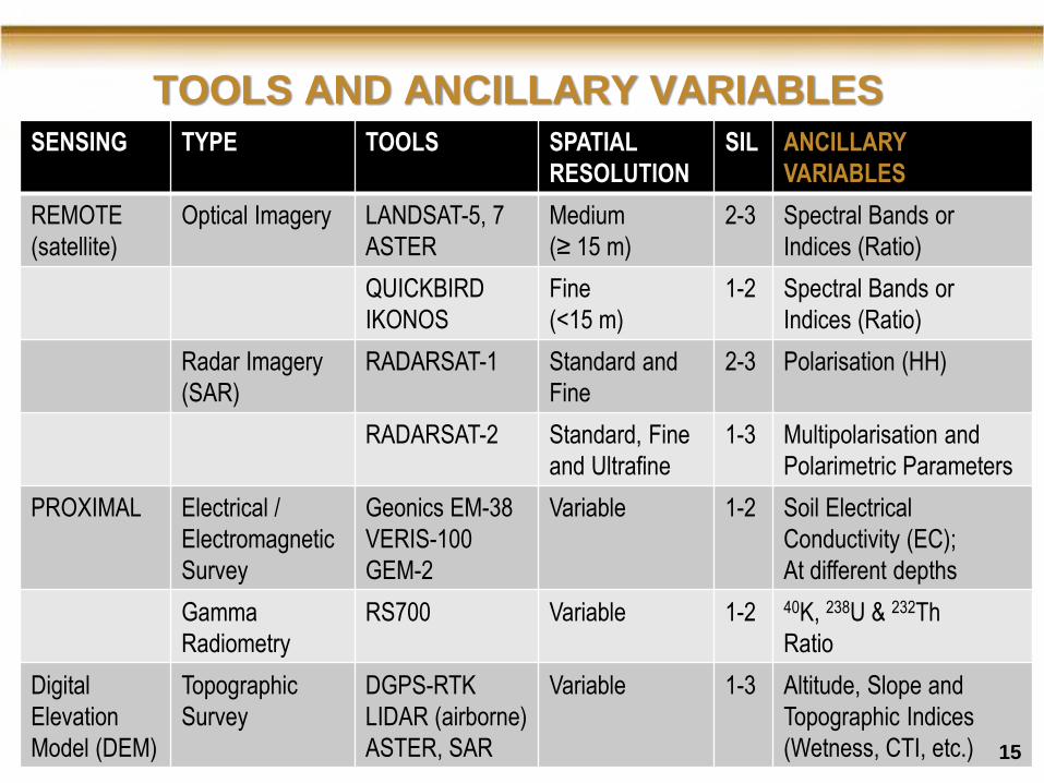
TOOLS AND ANCILLARY VARIABLES SENSING TYPE TOOLS SPATIAL
RESOLUTION
SIL ANCILLARY
VARIABLES
REMOTE
(satellite)
Optical Imagery LANDSAT-5, 7
ASTER
Medium
(≥ 15 m)
2-3 Spectral Bands or
Indices (Ratio)
QUICKBIRD
IKONOS
Fine
(<15 m)
1-2 Spectral Bands or
Indices (Ratio)
Radar Imagery
(SAR)
RADARSAT-1 Standard and
Fine
2-3 Polarisation (HH)
RADARSAT-2
Standard, Fine
and Ultrafine
1-3 Multipolarisation and
Polarimetric Parameters
PROXIMAL Electrical /
Electromagnetic
Survey
Geonics EM-38
VERIS-100
GEM-2
Variable 1-2 Soil Electrical
Conductivity (EC);
At different depths
Gamma
Radiometry
RS700 Variable
1-2 40K, 238U & 232Th
Ratio
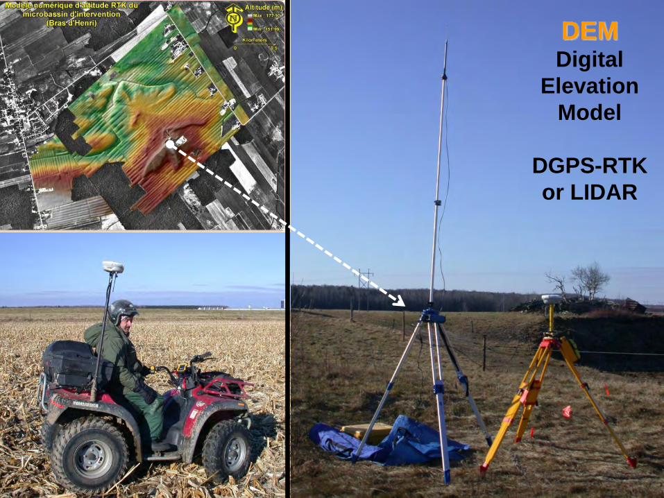
Digital
Elevation
Model (DEM)
Topographic
Survey
DGPS-RTK
LIDAR (airborne)
ASTER, SAR
Variable
1-3
Altitude, Slope and
Topographic Indices
(Wetness, CTI, etc.) 15
16
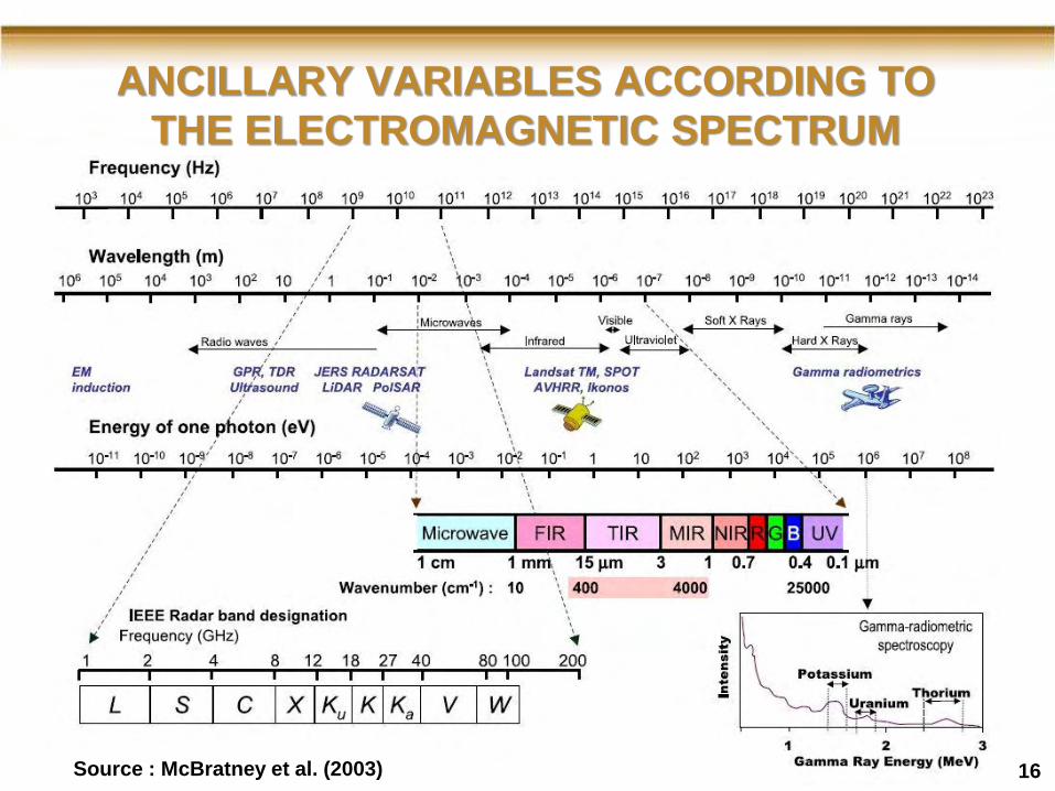
ANCILLARY VARIABLES ACCORDING TO
THE ELECTROMAGNETIC SPECTRUM
Source : McBratney et al. (2003)
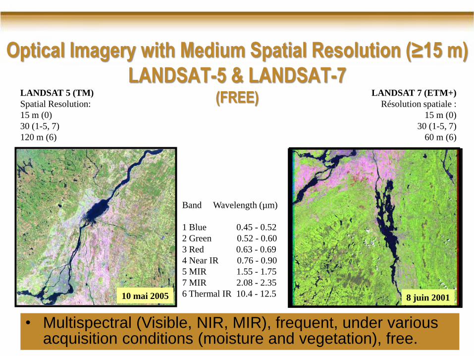
Optical Imagery with Medium Spatial Resolution (≥15 m)
LANDSAT-5 & LANDSAT-7 (FREE)
• Multispectral (Visible, NIR, MIR), frequent, under various acquisition conditions (moisture and vegetation), free.
10 mai 2005
LANDSAT 5 (TM)
Spatial Resolution:
15 m (0)
30 (1-5, 7)
120 m (6)
Band Wavelength (µm)
1 Blue 0.45 - 0.52
2 Green 0.52 - 0.60
3 Red 0.63 - 0.69
4 Near IR 0.76 - 0.90
5 MIR 1.55 - 1.75
7 MIR 2.08 - 2.35
6 Thermal IR 10.4 - 12.5 8 juin 2001
LANDSAT 7 (ETM+)
Résolution spatiale :
15 m (0)
30 (1-5, 7)
60 m (6)
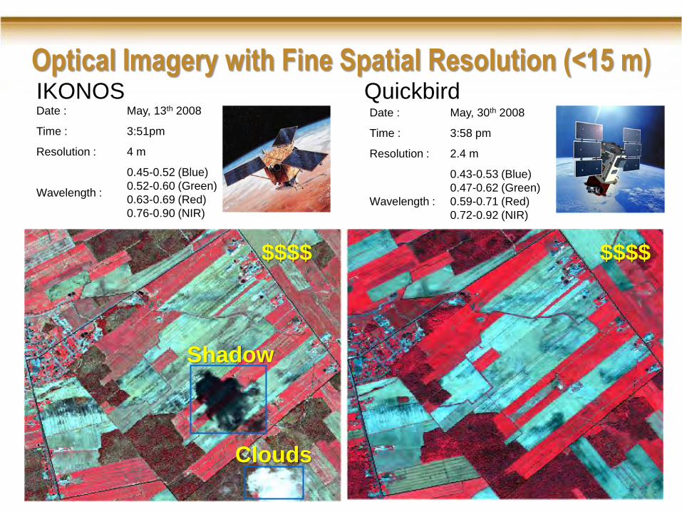
Date : May, 30th 2008
Time : 3:58 pm
Resolution : 2.4 m
Wavelength :
0.43-0.53 (Blue)
0.47-0.62 (Green)
0.59-0.71 (Red)
0.72-0.92 (NIR)
Date : May, 13th 2008
Time : 3:51pm
Resolution : 4 m
Wavelength :
0.45-0.52 (Blue)
0.52-0.60 (Green)
0.63-0.69 (Red)
0.76-0.90 (NIR)
IKONOS Quickbird
Optical Imagery with Fine Spatial Resolution (<15 m)
$$$$ $$$$
Shadow
Clouds
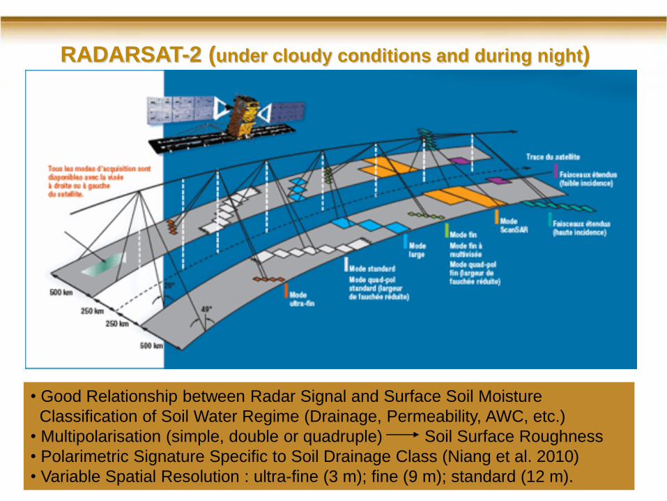
RADARSAT-2 (under cloudy conditions and during night)
• Good Relationship between Radar Signal and Surface Soil Moisture
Classification of Soil Water Regime (Drainage, Permeability, AWC, etc.)
• Multipolarisation (simple, double or quadruple) Soil Surface Roughness
• Polarimetric Signature Specific to Soil Drainage Class (Niang et al. 2010)
• Variable Spatial Resolution : ultra-fine (3 m); fine (9 m); standard (12 m).
21
A
B
C
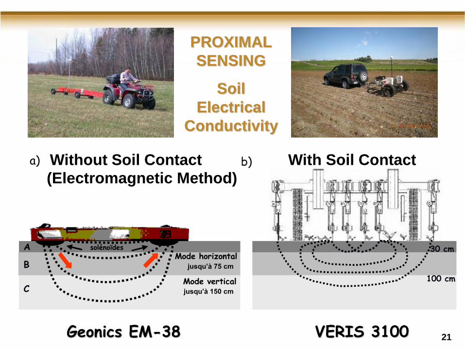
30 cm
100 cm
Mode horizontal
Mode vertical
jusqu’à 75 cm
jusqu’à 150 cm
a) b)
solénoïdes
PROXIMAL
SENSING
Soil
Electrical
Conductivity
Geonics EM-38 VERIS 3100
Without Soil Contact With Soil Contact
(Electromagnetic Method)
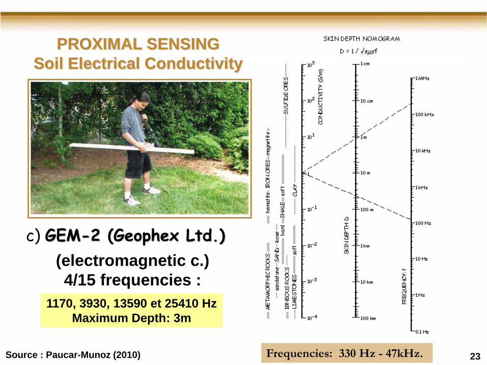
c) GEM-2 (Geophex Ltd.)
(electromagnetic c.)
4/15 frequencies :
Frequencies: 330 Hz - 47kHz. Source : Paucar-Munoz (2010) 23
1170, 3930, 13590 et 25410 Hz
Maximum Depth: 3m
PROXIMAL SENSING
Soil Electrical Conductivity
24
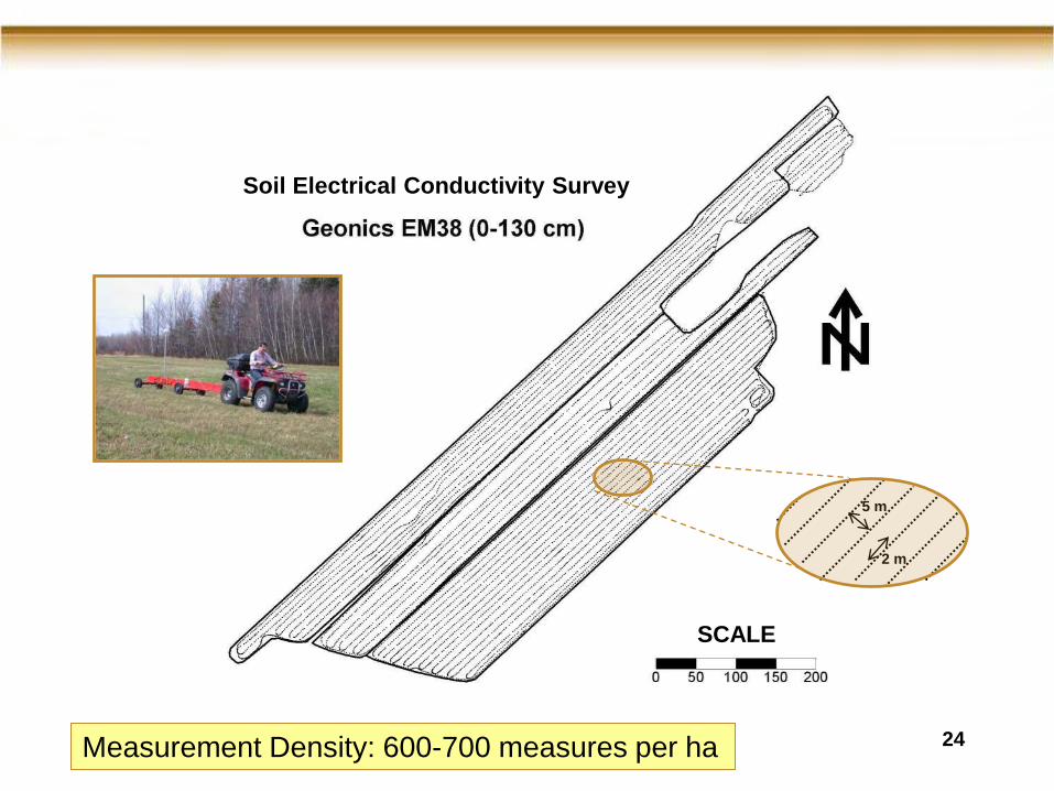
5 m
2 m
Measurement Density: 600-700 measures per ha
SCALE
Soil Electrical Conductivity Survey
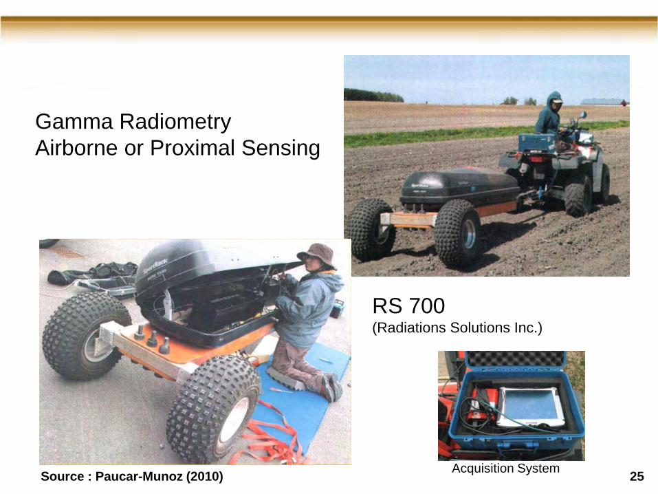
Source : Paucar-Munoz (2010) 25
RS 700 (Radiations Solutions Inc.)
Acquisition System
Gamma Radiometry
Airborne or Proximal Sensing
26
DEM Digital
Elevation
Model
DGPS-RTK
or LIDAR
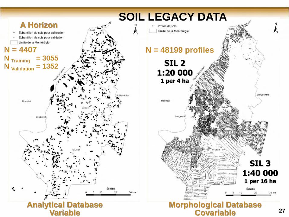
Analytical Database Variable
Morphological Database Covariable
N = 4407 N Training = 3055 N Validation = 1352
N = 48199 profiles
27
A Horizon SOIL LEGACY DATA
SIL 2 1:20 000
1 per 4 ha
SIL 3 1:40 000 1 per 16 ha
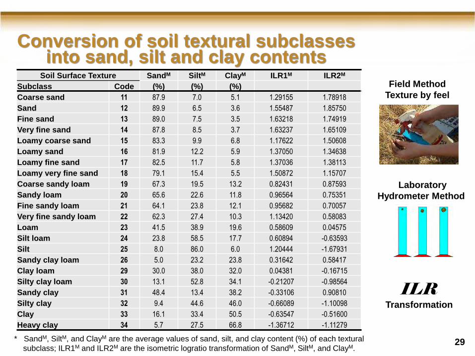
Conversion of soil textural subclasses into sand, silt and clay contents
Field Method
Texture by feel
Laboratory
Hydrometer Method
ILR Transformation
29
Soil Surface Texture SandM SiltM ClayM ILR1M ILR2M
Subclass Code (%) (%) (%)
Coarse sand 11 87.9 7.0 5.1 1.29155 1.78918
Sand 12 89.9 6.5 3.6 1.55487 1.85750
Fine sand 13 89.0 7.5 3.5 1.63218 1.74919
Very fine sand 14 87.8 8.5 3.7 1.63237 1.65109
Loamy coarse sand 15 83.3 9.9 6.8 1.17622 1.50608
Loamy sand 16 81.9 12.2 5.9 1.37050 1.34638
Loamy fine sand 17 82.5 11.7 5.8 1.37036 1.38113
Loamy very fine sand 18 79.1 15.4 5.5 1.50872 1.15707
Coarse sandy loam 19 67.3 19.5 13.2 0.82431 0.87593
Sandy loam 20 65.6 22.6 11.8 0.96564 0.75351
Fine sandy loam 21 64.1 23.8 12.1 0.95682 0.70057
Very fine sandy loam 22 62.3 27.4 10.3 1.13420 0.58083
Loam 23 41.5 38.9 19.6 0.58609 0.04575
Silt loam 24 23.8 58.5 17.7 0.60894 -0.63593
Silt 25 8.0 86.0 6.0 1.20444 -1.67931
Sandy clay loam 26 5.0 23.2 23.8 0.31642 0.58417
Clay loam 29 30.0 38.0 32.0 0.04381 -0.16715
Silty clay loam 30 13.1 52.8 34.1 -0.21207 -0.98564
Sandy clay 31 48.4 13.4 38.2 -0.33106 0.90810
Silty clay 32 9.4 44.6 46.0 -0.66089 -1.10098
Clay 33 16.1 33.4 50.5 -0.63547 -0.51600
Heavy clay 34 5.7 27.5 66.8 -1.36712 -1.11279
* SandM, SiltM, and ClayM are the average values of sand, silt, and clay content (%) of each textural
subclass; ILR1M and ILR2M are the isometric logratio transformation of SandM, SiltM, and ClayM.
30
DIGITAL SOIL MAPPING
SCALE-BASED RESULTS
(SIL 3 – SIL 2 – SIL 1)
31
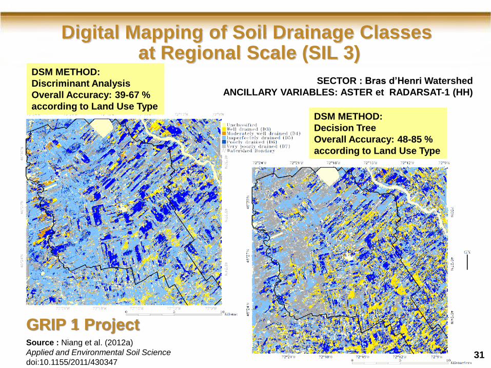
Digital Mapping of Soil Drainage Classes at Regional Scale (SIL 3)
Source : Niang et al. (AESS, accepté)
31
GRIP 1 Project
SECTOR : Bras d’Henri Watershed
ANCILLARY VARIABLES: ASTER et RADARSAT-1 (HH)
DSM METHOD:
Decision Tree
Overall Accuracy: 48-85 %
according to Land Use Type
DSM METHOD:
Discriminant Analysis
Overall Accuracy: 39-67 %
according to Land Use Type
Source : Niang et al. (2012a)
Applied and Environmental Soil Science
doi:10.1155/2011/430347
33
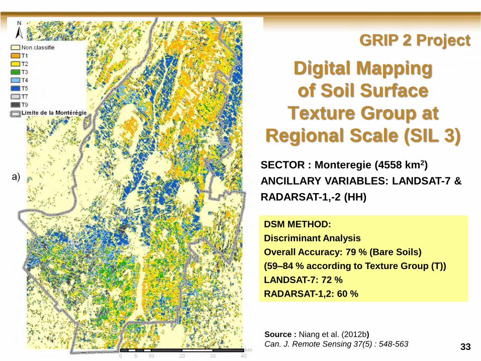
Digital Mapping
of Soil Surface
Texture Group at
Regional Scale (SIL 3)
GRIP 2 Project
SECTOR : Monteregie (4558 km2)
ANCILLARY VARIABLES: LANDSAT-7 &
RADARSAT-1,-2 (HH)
DSM METHOD:
Discriminant Analysis
Overall Accuracy: 79 % (Bare Soils)
(59–84 % according to Texture Group (T))
LANDSAT-7: 72 %
RADARSAT-1,2: 60 %
Source : Niang et al. (2012b)
Can. J. Remote Sensing 37(5) : 548-563
34
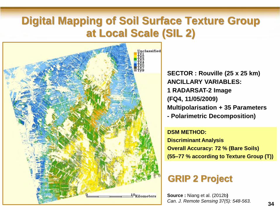
GRIP 2 Project
SECTOR : Rouville (25 x 25 km)
ANCILLARY VARIABLES:
1 RADARSAT-2 Image
(FQ4, 11/05/2009)
Multipolarisation + 35 Parameters
- Polarimetric Decomposition)
DSM METHOD:
Discriminant Analysis
Overall Accuracy: 72 % (Bare Soils)
(55–77 % according to Texture Group (T))
Source : Niang et al. (2012b)
Can. J. Remote Sensing 37(5): 548-563.
Digital Mapping of Soil Surface Texture Group at Local Scale (SIL 2)
35
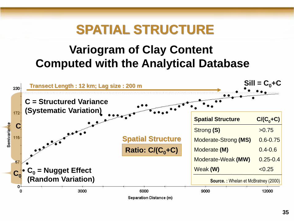
Variogram of Clay Content
Computed with the Analytical Database
Transect Length : 12 km; Lag size : 200 m
C0
C
C0 = Nugget Effect
(Random Variation)
C = Structured Variance
(Systematic Variation)
Ratio: C/(C0+C)
Sill = C0+C
Spatial Structure
Source. : Whelan et McBratney (2000)
<0.25 Weak (W)
0.25-0.4 Moderate-Weak (MW)
0.4-0.6 Moderate (M)
0.6-0.75 Moderate-Strong (MS)
>0.75 Strong (S)
C/(C0+C) Spatial Structure
SPATIAL STRUCTURE
• The Spatial Structure of Primary Soil Properties in Monteregie
present is strong (C/(C0+C)=0.81-0.96).
• Excellent for producing DSM with geostatistical methods.
RESULTS
37
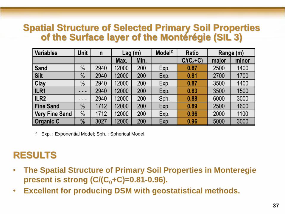
Spatial Structure of Selected Primary Soil Properties of the Surface layer of the Montérégie (SIL 3)
Variables Unit n Lag (m) ModelZ Ratio Range (m)
Max. Min. C/(C0+C) major minor
Sand % 2940 12000 200 Exp. 0.87 2500 1400
Silt % 2940 12000 200 Exp. 0.81 2700 1700
Clay % 2940 12000 200 Exp. 0.87 3500 1400
ILR1 - - - 2940 12000 200 Exp. 0.83 3500 1500
ILR2 - - - 2940 12000 200 Sph. 0.88 6000 3000
Fine Sand % 1712 12000 200 Exp. 0.89 2500 1600
Very Fine Sand % 1712 12000 200 Exp. 0.96 2000 1100
Organic C % 3027 12000 200 Exp. 0.96 5000 3000
Z Exp. : Exponential Model; Sph. : Spherical Model.
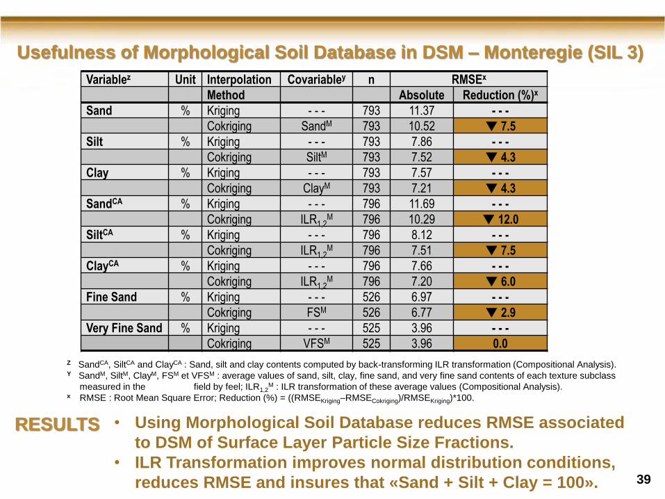
• Using Morphological Soil Database reduces RMSE associated
to DSM of Surface Layer Particle Size Fractions.
• ILR Transformation improves normal distribution conditions,
reduces RMSE and insures that «Sand + Silt + Clay = 100».
RESULTS
Usefulness of Morphological Soil Database in DSM – Monteregie (SIL 3)
39
Variablez Unit Interpolation Covariabley n RMSEx
Method Absolute Reduction (%)x
Sand % Kriging - - - 793 11.37 - - -
Cokriging SandM 793 10.52 ▼ 7.5
Silt % Kriging - - - 793 7.86 - - -
Cokriging SiltM 793 7.52 ▼ 4.3
Clay % Kriging - - - 793 7.57 - - -
Cokriging ClayM 793 7.21 ▼ 4.3
SandCA % Kriging - - - 796 11.69 - - -
Cokriging ILR1,2M 796 10.29 ▼ 12.0
SiltCA % Kriging - - - 796 8.12 - - -
Cokriging ILR1,2M 796 7.51 ▼ 7.5
ClayCA % Kriging - - - 796 7.66 - - -
Cokriging ILR1,2M 796 7.20 ▼ 6.0
Fine Sand % Kriging - - - 526 6.97 - - -
Cokriging FSM 526 6.77 ▼ 2.9
Very Fine Sand % Kriging - - - 525 3.96 - - -
Cokriging VFSM 525 3.96 0.0
Z SandCA, SiltCA and ClayCA : Sand, silt and clay contents computed by back-transforming ILR transformation (Compositional Analysis). Y SandM, SiltM, ClayM, FSM et VFSM : average values of sand, silt, clay, fine sand, and very fine sand contents of each texture subclass
measured in the field by feel; ILR1,2M : ILR transformation of these average values (Compositional Analysis).
x RMSE : Root Mean Square Error; Reduction (%) = ((RMSEKriging–RMSECokriging)/RMSEKriging)*100.
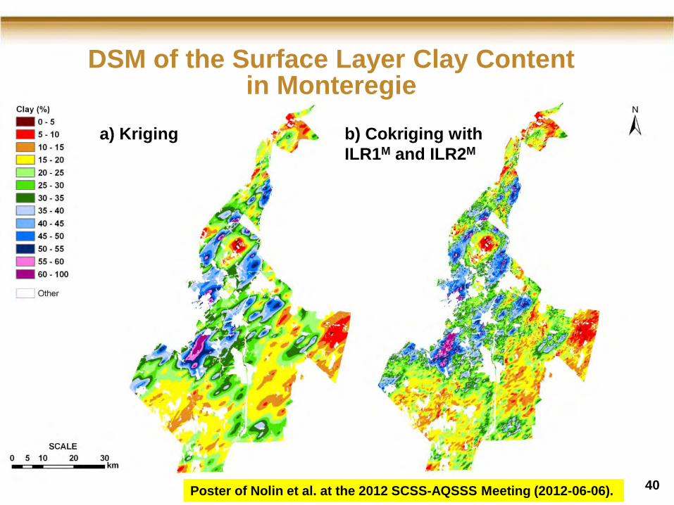
DSM of the Surface Layer Clay Content in Monteregie
40
a) Kriging b) Cokriging with
ILR1M and ILR2M
Poster of Nolin et al. at the 2012 SCSS-AQSSS Meeting (2012-06-06).
0 2,5 5 7,5 km
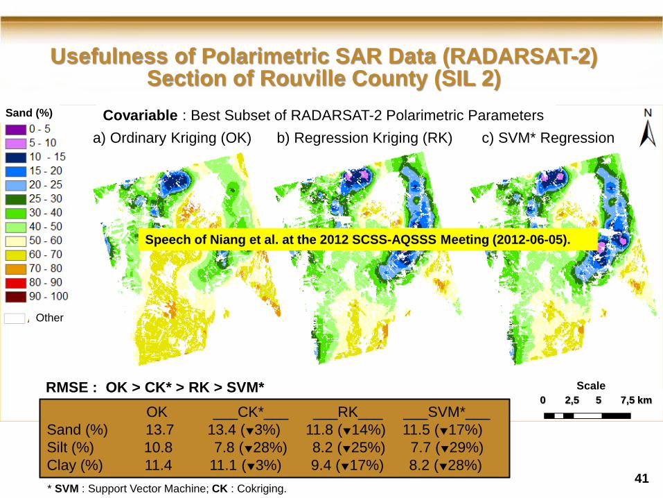
Covariable : Best Subset of RADARSAT-2 Polarimetric Parameters
41
a) Ordinary Kriging (OK) b) Regression Kriging (RK) c) SVM* Regression
Sand (%)
Other
Scale
OK ___CK*___ ___RK___ ___SVM*___
Sand (%) 13.7 13.4 (▼3%) 11.8 (▼14%) 11.5 (▼17%)
Silt (%) 10.8 7.8 (▼28%) 8.2 (▼25%) 7.7 (▼29%)
Clay (%) 11.4 11.1 (▼3%) 9.4 (▼17%) 8.2 (▼28%)
RMSE : OK > CK* > RK > SVM*
Usefulness of Polarimetric SAR Data (RADARSAT-2) Section of Rouville County (SIL 2)
* SVM : Support Vector Machine; CK : Cokriging.
Speech of Niang et al. at the 2012 SCSS-AQSSS Meeting (2012-06-05).
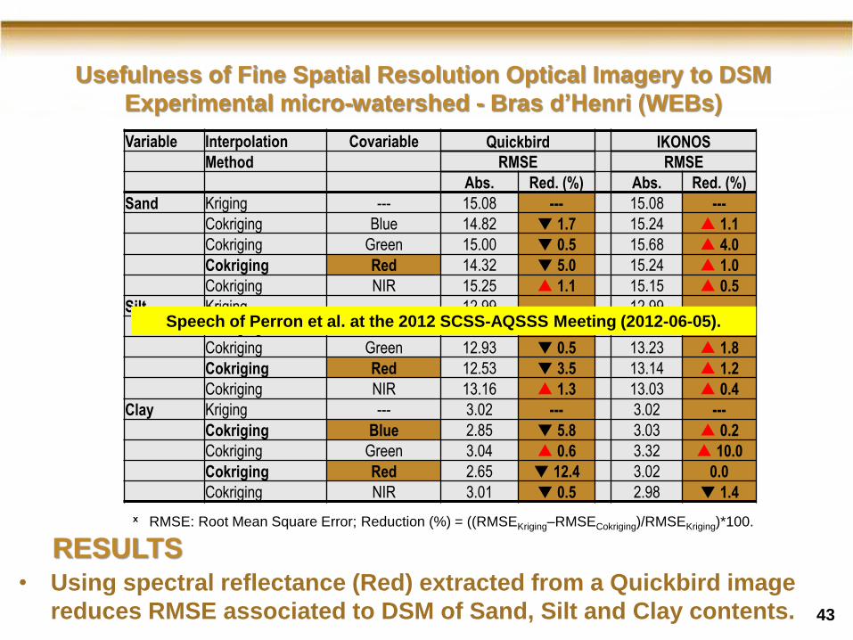
Usefulness of Fine Spatial Resolution Optical Imagery to DSM
Experimental micro-watershed - Bras d’Henri (WEBs)
• Using spectral reflectance (Red) extracted from a Quickbird image
reduces RMSE associated to DSM of Sand, Silt and Clay contents.
RESULTS
43
Variable Interpolation Covariable Quickbird IKONOS
Method RMSE RMSE
Abs. Red. (%) Abs. Red. (%)
Sand Kriging --- 15.08 --- 15.08 ---
Cokriging Blue 14.82 ▼ 1.7 15.24 ▲ 1.1
Cokriging Green 15.00 ▼ 0.5 15.68 ▲ 4.0
Cokriging Red 14.32 ▼ 5.0 15.24 ▲ 1.0
Cokriging NIR 15.25 ▲ 1.1 15.15 ▲ 0.5
Silt Kriging --- 12.99 --- 12.99 ---
Cokriging Blue 12.86 ▼ 1.0 13.14 ▲ 1.2
Cokriging Green 12.93 ▼ 0.5 13.23 ▲ 1.8
Cokriging Red 12.53 ▼ 3.5 13.14 ▲ 1.2
Cokriging NIR 13.16 ▲ 1.3 13.03 ▲ 0.4
Clay Kriging --- 3.02 --- 3.02 ---
Cokriging Blue 2.85 ▼ 5.8 3.03 ▲ 0.2
Cokriging Green 3.04 ▲ 0.6 3.32 ▲ 10.0
Cokriging Red 2.65 ▼ 12.4 3.02 0.0
Cokriging NIR 3.01 ▼ 0.5 2.98 ▼ 1.4
x RMSE: Root Mean Square Error; Reduction (%) = ((RMSEKriging–RMSECokriging)/RMSEKriging)*100.
Speech of Perron et al. at the 2012 SCSS-AQSSS Meeting (2012-06-05).
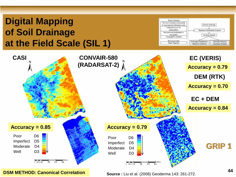
Digital Mapping
of Soil Drainage
at the Field Scale (SIL 1)
CASI CONVAIR-580
(RADARSAT-2)
DSM METHOD: Canonical Correlation
Accuracy = 0.85 Accuracy = 0.79
Source : Liu et al. (2008) Geoderma 143: 261-272.
Poor D6
Imperfect D5
Moderate D4
Well D3
EC (VERIS)
Accuracy = 0.79
DEM (RTK)
Accuracy = 0.70
EC + DEM
Accuracy = 0.84
GRIP 1
Poor D6
Imperfect D5
Moderate D4
Well D3
44
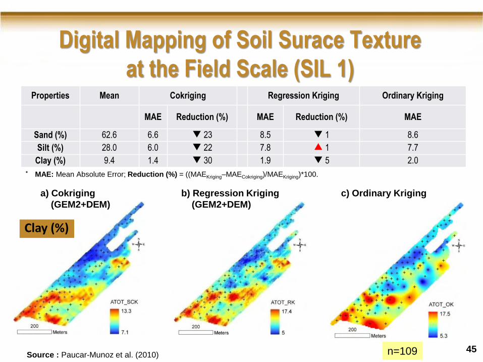
Digital Mapping of Soil Surace Texture
at the Field Scale (SIL 1)
Source : Paucar-Munoz et al. (2010) n=109
Clay (%)
c) Ordinary Kriging a) Cokriging
(GEM2+DEM)
b) Regression Kriging
(GEM2+DEM)
Properties Mean Cokriging Regression Kriging Ordinary Kriging
MAE Reduction (%) MAE Reduction (%) MAE
Sand (%) 62.6 6.6 ▼ 23 8.5 ▼ 1 8.6
Silt (%) 28.0 6.0 ▼ 22 7.8 ▲ 1 7.7
Clay (%) 9.4 1.4 ▼ 30 1.9 ▼ 5 2.0
45
* MAE: Mean Absolute Error; Reduction (%) = ((MAEKriging–MAECokriging)/MAEKriging)*100.
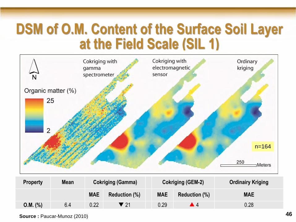
DSM of O.M. Content of the Surface Soil Layer at the Field Scale (SIL 1)
Source : Paucar-Munoz (2010)
n=164
46
Property Mean Cokriging (Gamma) Cokriging (GEM-2) Ordinairy Kriging
MAE Reduction (%) MAE Reduction (%) MAE
O.M. (%) 6.4 0.22 ▼ 21 0.29 ▲ 4 0.28
49
Conclusions • Using Ancillary Variables (Soil Legacy Data, DEM,
Remote & Proximal Sensing) significantly improves
the precision of DSM (reduces Error) – Choosing the
Best Strategy according to the scale (SIL), Data
available, Cost and Study Area Variability.
• DSM Precision is also a function of Spatial Inference
Models – SPATIAL STRUCTURE NEEDED
• Future Works: Efficient Sampling Strategy (Minimum
Sample Number)
• DSM improves Traditional Soil Survey Data to better
answer Users’ Needs.

“The difficulty lies, not in the new ideas, but in escaping the old ones”
John Maynard Keynes
GRIP
10MOA01001
Thank You!
• Isabelle, Mohamed, André, Mario, Lucie, Marie-Line, Suzanne … • Luc, Regis, Athyna, Noura, Éric, Xiaoyuan, Elizabeth, Scott … • AAFC,CS A, University (INRS-ETE, UQAM, Laval, Sherbrooke,
Students), MAPAQ, IRDA, Industry, CLUB, Farmers …
R.W. Baril, M.P. Cescas, D. Carrier & J.C. Dubé …