Embed Size (px)
Citation preview

The Enhanced Transitional Jobs Demonstration
New Perspectives on Creating Jobs Final Impacts of the Next Generation of
Subsidized Employment Programs
Bret Barden Randall Juras
Cindy Redcross Mary Farrell Dan Bloom
May 2018
The work in this publication was performed under Contract No. GS-10F-0245N awarded by the U.S. Department of Labor (DOL). For the Atlanta and San Francisco sites, research was per-formed under Contract No. HHSP23320100029YC, awarded by the U.S. Department of Health and Human Services (HHS).
The content of this publication does not necessarily reflect the views or policies of DOL or HHS, nor does mention of trade names, commercial practices, or organizations imply endorsement by the U.S. government.

iii
Overview
Some adults have great difficulty finding and holding jobs even when overall economic conditions are good. These individuals typically have low levels of formal education and skills, and other characteristics such as criminal records that place them at the back of the queue for job openings. Many programs have been developed to assist hard-to-employ job seekers, but few have demonstrated sustained success. One such model, “transitional jobs,” offers temporary jobs, subsidized with public funds, that aim to teach participants basic work skills or help them get a foot in the door with an employer. Several transitional jobs programs have been evaluated, with mixed results.
The Enhanced Transitional Jobs Demonstration (ETJD), funded by the Employment and Training Administra-tion of the U.S. Department of Labor, tested seven transitional jobs programs that targeted people recently re-leased from prison or low-income parents who had fallen behind in child support payments. The ETJD programs were “enhanced” in various ways relative to programs studied in the past. MDRC, a nonprofit, nonpartisan re-search organization, led the project along with two partners: Abt Associates and MEF Associates. The Office of Planning, Research, and Evaluation in the U.S. Department of Health and Human Services’ Administration for Children and Families also supported the evaluation.
The evaluation used a random assignment research design. Program group members were given access to the ETJD programs and control group members had access to other services in the community. This report presents the final impact results from the study 30 months after enrollment and information about the costs of the ETJD programs. Most measures presented in the report focus on the final year of the follow-up period, when nearly all program group members had left transitional jobs. The results therefore reflect longer-term effects of the pro-grams after the subsidized positions ended.
•
•
•
•
•
The ETJD programs increased participants’ earnings and employment rates in the final year of the study period. The program group earned about $700 more than the control group in that year. Sixty-four percent of the program group worked in that year, compared with 60 percent of the control group. Impacts on longer-term employment outcomes are better than those found in previous evaluations.
The three ETJD programs targeting people returning from prison reduced incarceration in prison among those at higher risk of reoffending. Although there was no statistically significant impact on a broad measure of recidivism (the rate at which people commit new crimes or are reincarcerated), there were some encouraging patterns on other measures of recidivism. In addition, among higher-risk participants across the three locations, there was a statistically significant reduction in incarceration in prison (of 12 percentage points) in the 30 months following study enrollment. The impacts on recidivism largely reflect the program in Indianapolis, which targeted a very disadvantaged and high-risk population.
The ETJD programs targeting noncustodial parents did not increase the amount of child support paid in the last year of the follow-up period. However, they did increase the proportion of parents who paid at least some support during this period by 6 percentage points.
Results varied somewhat among the programs. Some of the ETJD programs produced statistically sig-nificant effects on notable outcome measures. However, it is unclear whether patterns in results reflect dif-ferences in models, in the implementation of the models, in contextual factors, or in the characteristics of the ETJD sample members served in each location.
ETJD program costs ranged from about $7,000 to $11,100 per program group member. The net costs of the ETJD programs (taking control group costs and non-ETJD costs into account) ranged from about $6,200 to $11,100 per person.

THIS PAGE INTENTIONALLY LEFT BLANK

v
Contents
Overview iii List of Exhibits vii Acknowledgments xiii Executive Summary ES-1
Chapter
1 Introduction 1 Background and Context 2 The ETJD Project and the Evaluation 3 The ETJD Programs 6 Characteristics of the Study Participants 9 Program Implementation 13 Findings in This Report 19
2 Impacts on Earnings, Employment, and Material Well-Being 21 Confirmatory Analysis 21 Exploratory Analysis 22
3 Impacts on Child Support and Family Engagement 41 Confirmatory Analysis 41 Exploratory Analysis 43
4 Impacts on Recidivism 55 Confirmatory Analysis 55 Exploratory Analysis 55
5 Cost Analysis 67 Method 67 ETJD Costs 72 Net Costs 72 Was ETJD Cost-Effective? 76
6 Conclusion 79 Were the ETJD Programs Really “Enhanced”? 79 Were the ETJD Programs More Effective Than Earlier Transitional Jobs
Models? 80 Which ETJD Models Were the Most Effective? 81 What Are the Implications of ETJD for Policy, Practice, and Research? 82

vi
Appendix
A Subgroup Analyses 87
B Supplementary Tables and Figures for Atlanta 99
C Supplementary Tables and Figures for Milwaukee 115
D Supplementary Tables and Figures for San Francisco 131
E Supplementary Tables and Figures for Syracuse 147
F Supplementary Tables and Figures for Fort Worth 163
G Supplementary Tables and Figures for Indianapolis 177
H Supplementary Tables and Figures for New York City 191
I Baseline Characteristics of the Study Sample 205
J Selected Measures of Well-Being, by Site 219
K Survey Response Analysis 225
L The Analytic Approach to Determining Impacts on Recidivism-Risk Subgroups 245
M Extended Follow-Up 251
References 255
Earlier Reports on the Enhanced Transitional Jobs Demonstration 259
vii
List of Exhibits
Table
ES.1 ETJD Individual Program Characteristics ES-3
ES.2 Results of the Confirmatory Analysis ES-7
ES.3 Selected Results from the Exploratory Analysis ES-11
ES.4 Selected Site-Specific Findings ES-14
1.1 ETJD Individual Program Characteristics 8
1.2 Description of ETJD Enhancements 9
1.3 Selected Characteristics of Sample Members 12
2.1 Confirmatory Impact Measure for the Employment and Earnings Domain: All Sites 22
2.2 Impacts on Employment and Earnings: All Sites 24
2.3 Impacts on Material Hardship: All Sites 37
2.4 Impacts on Health, Well-Being, and Social Support: All Sites 38
3.1 Confirmatory Impact Measure for the Child Support Domain: Noncustodial Parent Sites 42
3.2 Impacts on Child Support and Family Relationships: Noncustodial Parent Sites 43
4.1 Confirmatory Impact Measure for the Criminal Justice Domain: Sites Targeting Formerly Incarcerated Individuals 56
4.2 Impacts on Criminal Justice Outcomes: Sites Targeting Formerly Incarcerated Individuals 57
4.3 Impacts on Criminal Justice Outcomes, by Site: Sites Targeting Formerly Incarcerated Individuals 61
4.4 Impacts on Criminal Justice Outcomes, by Recidivism Risk: Sites Targeting Formerly Incarcerated Individuals 65
5.1 Estimated ETJD Costs per Program Group Member (in 2016 Dollars) 73
5.2 Estimated Net Costs per Program Group Member (in 2016 Dollars) 74
5.3 Net Costs (in 2016 Dollars) Compared with Confirmatory Outcomes 78

viii
A.1 Impacts on Employment and Earnings, by Sites’ Target Populations 89
A.2 Impacts on Employment and Earnings Among Noncustodial Parents and Others: All Sites 90
A.3 Impacts on Employment and Earnings by Employment Status in the Year Before Entering the Study: Noncustodial Parent Sites 91
A.4 Impacts on Employment and Earnings, Child Support, and Criminal Justice Outcomes, by Level of Education 92
A.5 Impacts on Employment and Earnings, Child Support, and Criminal Justice Outcomes, by Age 94
A.6 Impacts on Employment and Earnings, Child Support, and Criminal Justice Outcomes, by Time of Entry into the Program 96
B.1 Impacts on Employment and Earnings: Atlanta 101
B.2 Impacts on Child Support and Family Relationships: Atlanta 103
B.3 Impacts on Criminal Justice Outcomes: Atlanta 105
B.4 Impacts on Material Hardship: Atlanta 106
B.5 Impacts on Health, Well-Being, and Social Support: Atlanta 107
C.1 Impacts on Employment and Earnings: Milwaukee 117
C.2 Impacts on Child Support and Family Relationships: Milwaukee 119
C.3 Impacts on Criminal Justice Outcomes: Milwaukee 121
C.4 Impacts on Material Hardship: Milwaukee 122
C.5 Impacts on Health, Well-Being, and Social Support: Milwaukee 123
D.1 Impacts on Employment and Earnings: San Francisco 133
D.2 Impacts on Child Support and Family Relationships: San Francisco 135
D.3 Impacts on Criminal Justice Outcomes: San Francisco 137
D.4 Impacts on Material Hardship: San Francisco 138
D.5 Impacts on Health, Well-Being, and Social Support: San Francisco 139
E.1 Impacts on Employment and Earnings: Syracuse 149
E.2 Impacts on Child Support and Family Relationships: Syracuse 151
E.3 Impacts on Criminal Justice Outcomes: Syracuse 153

ix
E.4 Impacts on Material Hardship: Syracuse 154
E.5 Impacts on Health, Well-Being, and Social Support: Syracuse 155
F.1 Impacts on Employment and Earnings: Fort Worth 165
F.2 Impacts on Criminal Justice Outcomes: Fort Worth 167
F.3 Impacts on Criminal Justice Outcomes, by Recidivism Risk: Fort Worth 168
F.4 Impacts on Child Support Among Participants Who Were Noncustodial Parents When They Entered the Study: Fort Worth 170
F.5 Impacts on Material Hardship: Fort Worth 171
F.6 Impacts on Health, Well-Being, and Social Support: Fort Worth 172
G.1 Impacts on Employment and Earnings: Indianapolis 179
G.2 Impacts on Criminal Justice Outcomes: Indianapolis 181
G.3 Impacts on Criminal Justice Outcomes, by Recidivism Risk: Indianapolis 182
G.4 Impacts on Child Support Among Participants Who Were Noncustodial Parents When They Entered the Study: Indianapolis 184
G.5 Impacts on Material Hardship: Indianapolis 185
G.6 Impacts on Health, Well-Being, and Social Support: Indiana 186
H.1 Impacts on Employment and Earnings: New York City 193
H.2 Impacts on Criminal Justice Outcomes: New York City 195
H.3 Impacts on Criminal Justice Outcomes, by Recidivism Risk: New York City 196
H.4 Impacts on Child Support Among Participants Who Were Noncustodial Parents When They Entered the Study: New York City 198
H.5 Impacts on Material Hardship: New York City 199
H.6 Impacts on Health, Well-Being, and Social Support: New York City 200
I.1 Characteristics and Employment Histories of Sample Members: Noncustodial Parent Sites 207
I.2 Child Support and Criminal Justice Characteristics of Sample Members: Noncustodial Parent Sites 209
I.3 Additional Characteristics of Sample Members at Enrollment: Noncustodial Parent Sites 211

x
I.4 Characteristics and Employment Histories of Sample Members: Sites Targeting Formerly Incarcerated Individuals 213
I.5 Child Support and Criminal Justice Characteristics of Sample Members: Sites Targeting Formerly Incarcerated Individuals 215
I.6 Additional Characteristics of Sample Members at Enrollment: Sites Targeting Formerly Incarcerated Individuals 216
K.1 ETJD 30-Month Survey Response Rates 231
K.2 Selected Baseline Characteristics of ETJD 30-Month Survey Respondents and Nonrespondents, by City 232
K.3 Selected Baseline Characteristics of ETJD 30-Month Survey Respondents, by Research Group and City 236
K.4 Impacts on Employment and Earnings Among Survey Respondents and the Full Sample 240
Figure
ES.1 Employment and Earnings Over Time: All Sites ES-9
1.1 Generic Logic Model 11
1.2 Subsidized Employment in the ETJD Programs 15
1.3 Impacts on Receipt of Employment Services, by Site 16
2.1 Employment and Earnings Over Time: All Sites 26
2.2 Percentage Employed Over the Last Year of the Follow-Up Period, by Site 28
2.3 Earnings Over the Last Year of the Follow-Up Period, by Site 30
2.4 Earnings Over Time: Noncustodial Parent Sites 31
2.5 Earnings Over Time: Sites Targeting Formerly Incarcerated Individuals 32
3.1 Child Support Payment Over Time: Noncustodial Parent Sites 45
3.2 Payment of Child Support in the Last Year of the Follow-Up Period: Noncustodial Parent Sites 47
3.3 Amount of Child Support Paid Over Time: Noncustodial Parent Sites 49
3.4 Contact and Interactions with the Focal Child: Noncustodial Parent Sites 50
3.5 Closeness to the Focal Child: Noncustodial Parent Sites 51
xi
3.6 Involvement in Parenting Decisions for the Focal Child: Noncustodial Parent Sites 52
4.1 Percentage Arrested, Convicted, or Admitted to Jail or Prison, by Site 59
5.1 Cost Components 69
B.1 Employment and Earnings Over Time: Atlanta 108
B.2 Employment and Earnings Over Time (Extended Follow-Up): Atlanta 110
B.3 Child Support Payment Over Time: Atlanta 112
C.1 Employment and Earnings Over Time: Milwaukee 124
C.2 Employment and Earnings Over Time (Extended Follow-Up): Milwaukee 126
C.3 Child Support Payment Over Time: Milwaukee 128
D.1 Employment and Earnings Over Time: San Francisco 140
D.2 Employment and Earnings Over Time (Extended Follow-Up): San Francisco 142
D.3 Child Support Payment Over Time: San Francisco 144
E.1 Employment and Earnings Over Time: Syracuse 156
E.2 Employment and Earnings Over Time (Extended Follow-Up): Syracuse 158
E.3 Child Support Payment Over Time: Syracuse 160
F.1 Employment and Earnings Over Time: Fort Worth 173
F.2 Employment and Earnings Over Time (Extended Follow-Up): Fort Worth 175
G.1 Employment and Earnings Over Time: Indianapolis 187
G.2 Employment and Earnings Over Time (Extended Follow-Up): Indianapolis 189
H.1 Employment and Earnings Over Time: New York City 201
H.2 Employment and Earnings Over Time (Extended Follow-Up): New York City 203
J.1 Experienced a Financial Shortfall in the Past 12 Months, by Site 221
J.2 Health Insurance in the Last Month, by Site 222
J.3 Food Stamp Receipt Over the Past Month, by Site 223
M.1 Employment and Earnings Over Time (Extended Follow-Up): All Sites 253
Box
1.1 Confirmatory and Exploratory Analyses 6

THIS PAGE INTENTIONALLY LEFT BLANK

xiii
Acknowledgments
The Enhanced Transitional Jobs Demonstration (ETJD) and this report would not be possible without the contributions of many people in the dozens of agencies and organizations participating in the project. We thank the funders at the U.S. Department of Labor (DOL) and the U.S. Department of Health and Human Services (HHS). In particular we thank Eileen Pederson, our DOL project officer, for her invaluable dedication and thoughtfulness throughout the project and for reviewing and providing comments on this report. We also thank Dan Ryan for his support and for reviewing and providing comments as well. We are grateful to Heidi Casta, Wayne Gordon, Jenn Smith, and Michelle Ennis for their contributions and commitment to the project. From HHS we thank Girley Wright, Erika Zielewski (who has since moved to the U.S. Office of Management and Budget), and Mark Fucello for their ongoing partnership and helpful collaboration on the project.
We are especially grateful to the hardworking and dedicated administrators and staff members in each of the seven ETJD programs who have given generously of their time throughout the project.
From Atlanta, Georgia: Jenny Taylor, Marylee Putnam, Cheryl Cornett-Earley, and Iana Kanazirska-Petkova.
From Fort Worth, Texas: Debby Kratky, John Torres, Christina Mason, Robert Sturgeon, and Jack Cummings.
From Indianapolis, Indiana: Gregg Keesling, Brent Matthews, Rhonda Shipley, Calvin Houston, Jannett Keesling, and Thomas Gray.
From Milwaukee, Wisconsin: Nyette Brown-Ellis, Reginald Riley, Marrika Rodgers, Robin Balfanz, and Jennifer de Montmollin.
From New York City, New York: Nadia Sadloski, Felipe Vargas, Valerie Westphal, Zachary Smith, Marion Kowalski, Angela Gerena, and Nathan Gunsch.
From San Francisco, California: at Goodwill, Megan Kenny, David Walker, and Elsie Wong; at the San Francisco Department of Child Support Services, Karen Roye, Christine Anderson, Sheryl Myers, and Freda Randolph Glenn; and at the Mayor’s Office of Economic and Workforce Development, John Halpin, Monique Forester, and Lisa Estrada.
From Syracuse, New York: Michael Pasquale, Marsha Weissman, David Condliffe, Christine Abate, and Michael Irwin.
From DOL, we are also grateful to the Regional Federal Project Officers that provided contractual and programmatic technical assistance to the ETJD grantees: in Atlanta, Georgia, Sherrie Wilson; in Fort Worth, Texas, Amanda Denogean; in Indianapolis, Indiana, and Milwaukee, Wisconsin, Darren Kroenke;

xiv
in New York City, New York, Rochelle Layne; in San Francisco, California, Elina Mnatsakanova; and in Syracuse, New York, Michael Hotard.
We thank the many staff members from state and local criminal justice and child support agencies that facilitated our access to the administrative data used in this report: the California Department of Child Support Services, the Georgia Division of Child Support Services in the Department of Human Services, the Texas Department of Public Safety, the Texas Department of Criminal Justice, the Tarrant County Sheriff’s Office, the Indiana State Police, the Indiana Department of Corrections, the Marion County Sheriff’s Office, the New York Division of Criminal Justice Statistics, the New York State Department of Corrections and Community Supervision, the New York City Department of Corrections, the New York State Office of Temporary and Disability Assistance’s Division of Child Support Enforcement, the Institute for Research on Poverty at the University of Wisconsin-Madison, and the Wisconsin Department of Children and Families. We also thank staff members from HHS and the Social Security Administration who worked to provide us with data from the National Directory of New Hires. The Center for Employment Opportunities graciously provided data to inform the analysis of the New York City program.
At MDRC, Jill Verrillo masterfully coordinated the report’s production and the creation of the report’s many exhibits with unwavering dedication, determination, and resourcefulness. Johanna Walter managed multiple aspects of data collection and processing and provided sound counsel on the analysis throughout the project. Beata Luczywek, Chloe Anderson, Danielle Cummings, Gary Reynolds, Melanie Skemer, and Sally Dai were part of the outstanding quantitative analysis team that skillfully processed the surveys and dozens of federal, state, and local administrative data sets for the analysis in this report. Nicole Morris and Lee Robeson led the survey management. Rick Hendra, Chuck Michalopoulos, and Gordon Berlin reviewed drafts of the report and offered insightful comments. Emily Brennan, Samuel Diaz, Molly Williams, Tejomay Gadgil, Abby Durgan, Vicky Ho, Zaina Rodney, and Justine Yu provided indispensable assistance in report production. Joshua Malbin expertly and efficiently edited and reviewed the report, and Carolyn Thomas and Ann Kottner prepared it for publication.
From MEF Associates, Claire Ma, Riley Webster, Kim Foley, and Emmi Obara were part of the stellar team that created and checked cost estimates and assisted with collection of cost data. From Abt Associates, Steve Bell reviewed multiple drafts of the report and provided thoughtful comments. From Abt Schulman, Ronca & Bucuvalas, Inc. (SRBI), Donna DeMarco, Jodi Walton, Ray Hildonen, and Ricki Jarmon led the survey administration effort. From Decision Information Resources, Inc., Jim Cooper, Lenin Williams, Monica Schneider, and Sylvia Epps led survey administration efforts.
Finally, we extend our deep appreciation to the thousands of men and women who participated in the study and gave generously of their time. They have contributed immeasurably to research that helps improve services and policy for noncustodial parents and formerly incarcerated individuals in the demonstration cities and beyond.
The Authors
ES-1
Executive Summary
Across the United States, some adults have great difficulty finding and holding jobs even when overall economic conditions are good. These individuals typically have low levels of formal education and skills and other characteristics such as criminal records that place them at the back of the queue for job openings.1
Many programs have been developed to assist hard-to-employ job seekers, but few have demonstrated sustained success. One model that has been implemented and tested fairly exten-sively is called “transitional jobs.” Some transitional jobs programs are designed primarily to provide work-based income support to jobless workers. Others offer temporary jobs, subsidized with public funds, that aim to teach participants basic work skills or help them get a foot in the door with an employer. Many of these programs also offer assistance with personal barriers that may hinder participants’ success, and help participants find permanent jobs. Previous evaluations of transitional jobs programs have found that the programs dramatically increased employment initially — demonstrating that they successfully targeted people who were unlikely to find jobs on their own — but the impacts faded after participants left the transitional jobs. The programs did not improve participants’ long-term employment outcomes. One program targeting people returning to the community from prison reduced recidivism (the rate at which former prisoners commit new crimes or are reincarcerated), but several other programs for the same population did not.2
This report presents the final results from the Enhanced Transitional Jobs Demonstration (ETJD), a large-scale research project sponsored by the Employment and Training Administra-tion (ETA) in the U.S. Department of Labor and also supported by the Administration for Chil-dren and Families (ACF) in the U.S. Department of Health and Human Services. In 2011, ETA held a national competition and selected seven organizations to operate transitional jobs programs
1Devah Pager, “The Mark of a Criminal Record,” American Journal of Sociology 108, 5 (2003): 937-975; Eleanor Krause and Isabel Sawhill, What We Know and Don't Know about Declining Labor Force Participation: A Review (Washington, DC: Brookings Institute, 2017); Harry J. Holzer, Steven Raphael, and Michael A. Stoll, “Employment Barriers Facing Ex-Offenders” (Washington, DC: Urban Institute, 2003); Martha Ross and Na-talie Holmes, Meet the Out-of-Work: Local Profiles of Jobless Adults and Strategies to Connect Them to Em-ployment (Washington, DC: Brookings Institute, 2017).
2Cindy Redcross, Megan Millenky, Timothy Rudd, and Valerie Levshin, More Than a Job: Final Results of the Center for Employment Opportunities (CEO) Transitional Jobs Program (New York: MDRC, 2012); David Butler, Julianna Alson, Dan Bloom, Victoria Deitch, Aaron Hill, JoAnn Hsueh, Erin Jacobs Valentine, Sue Kim, Reanin McRoberts, and Cindy Redcross, What Strategies Work for the Hard-to-Employ? Final Results of the Hard-to-Employ Demonstration and Evaluation Project and Selected Sites from the Employment Reten-tion and Advancement Project (New York: MDRC, 2012); Erin Jacobs Valentine, Returning to Work After Prison: Final Results from the Transitional Jobs Reentry Demonstration (New York: MDRC, 2012).
ES-2
targeting either low-income parents who did not live with one or more of their children (noncus-todial parents) and who owed child support, or individuals returning to the community from prison. Applicants were required to describe how their program would be “enhanced” relative to earlier transitional jobs programs that had been tested. Each of the selected organizations received about $6 million to recruit 1,000 individuals into the study and serve 500 of them. ETA awarded a contract to MDRC and its partners, Abt Associates and MEF Associates, to conduct a multifac-eted evaluation of the ETJD programs.3 An earlier report described the implementation of the ETJD programs and their effects on participants’ outcomes over 12 months.4 This report presents final results from the evaluation after 30 months, including results from a cost-effectiveness anal-ysis. The results are particularly relevant because transitional jobs are identified as an allowable activity under the Workforce Innovation and Opportunity Act (WIOA), the law that governs the nation’s public workforce system. Local WIOA programs may use up to 10 percent of their adult and dislocated worker funding to support transitional jobs for participants who are chronically unemployed or who have inconsistent work histories; individuals who have served time in prison are identified as a potential target group.5
Overall, the ETJD results are more encouraging than the earlier studies mentioned above. The programs increased both employment and earnings in the last year of the follow-up period, when nearly all program group members had left their transitional jobs. Results in the other two primary domains — criminal justice and child support — are more mixed, but in both there are positive results on some important outcome measures.
The ETJD Programs and Participants As shown in Table ES.1, four of the ETJD programs targeted noncustodial parents and three targeted formerly incarcerated individuals. Most of the programs were operated by private non-profit organizations, though they worked closely with local or state government agencies.
3ETA awarded a contract to a separate organization, Coffey Consulting, to provide programmatic technical assistance to the grantees.
4Cindy Redcross, Bret Barden, Dan Bloom, Joseph Broadus, Jennifer Thompson, Sonya Williams, Sam Elkin, Randall Juras, Janae Bonsu, Ada Tso, Barbara Fink, Whitney Engstrom, Johanna Walter, Gary Reynolds, Mary Farrell, Karen Gardiner, Arielle Sherman, Melanie Skemer, Yana Kusayeva, and Sara Muller-Ravett, Im-plementation and Early Impacts of the Next Generation of Subsidized Employment Programs (New York: MDRC, 2016).
5U.S. Department of Labor, Employment and Training Administration, “Employment and Training Admin-istration Advisory: Training and Employment Guidance Letter WIOA No. 3-15, Operating Guidance for the Workforce Innovation and Opportunity Act (Referred to as WIOA or the Opportunity Act)” (Website: https://wdr.doleta.gov/directives/attach/TEGL/TEGL_03-15.pdf, 2015).
ES-3
Table ES.1
ETJD Individual Program Characteristics
Location, Program Operator, and Name
Target Group Program Overview
Atlanta, GA Goodwill of North Georgia Good Transitions
Noncustodial parents
Participants worked at a Goodwill store for approximately one month, then moved into a less supported subsidized position with a private employer in the community for about three months. The program offered case management and short-term training.
Milwaukee, WI YWCA of Southeast Wisconsin Supporting Families Through Work
Noncustodial parents
Participants started in a three- to five-day job-readiness workshop. They were then placed in transitional jobs, mostly with private-sector employers. The program supplemented wages in unsubsidized employment to bring them up to $10 an hour for six months. The program also provided child support-related assistance.
San Francisco, CA Goodwill Industries, with San Francisco Dept. of Child Support Services TransitionsSF
Noncustodial parents
Participants began with an assessment followed by two weeks of job-readiness training. Then they were placed into one of three tiers of subsidized jobs depending on their job readiness: (1) nonprofit, private-sector jobs (mainly at Goodwill); (2) public-sector jobs; or (3) for-profit, private-sector jobs. They may have received modest financial incentives for participation milestones and child support assistance.
Syracuse, NY Center for Community Alternatives Parent Success Initiative
Noncustodial parents
Groups of 15-20 participants began the program together with a two-week job-readiness course. They were then placed in work crews with the local public housing authority, a business improvement district, or a nonprofit organization. The program offered family life-skills workshops, job-retention services, case management, civic restoration services, child support legal aid, and job-search and job-placement assistance.
Fort Worth, TX Workforce Solutions of Tarrant County Next STEP
Formerly incarcerated people
Participants began with a two-week “boot camp” that included assessments and job-readiness training. They were then placed in jobs with private employers. The program paid 100 percent of the wages for the first eight weeks and 50 percent for the following eight weeks. Employers were expected to retain participants who performed well. Other services included case management, group meetings, high school equivalency classes, and mental health services.
Indianapolis, IN RecycleForce, Inc. RecycleForce
Formerly incarcerated people
Participants were placed at one of three social enterprises, including an electronics recycling plant staffed by formerly incarcerated workers, who provided training and supervision to participants and served as their peer mentors. The program also offered occupational training, case management, job development, work-related financial support, and child support-related assistance. Participants may have been hired later as unsubsidized employees.
New York, NY The Doe Fund Ready, Willing and Able Pathways2Work
Formerly incarcerated people
After a one-week orientation, participants worked on the program’s street-cleaning crews for six weeks, then moved into subsidized internships for eight weeks. If an internship did not transition to unsubsidized employment, the program paid the participant to search for jobs for up to nine weeks. Additional services included case management, job-readiness programs, opportunities for short-term training and certification, and parenting and computer classes.
ES-4
The typical ETJD participant was a never-married black or Hispanic man between 30 and 40 years old, with a high school diploma or the equivalent but no postsecondary education. Al-most all of the study participants had worked in the past, but most had little recent work experi-ence. Studies have shown that African-American men, particularly those with criminal records, experience significant discrimination in the labor market.6 About 42 percent of the participants in the programs targeting formerly incarcerated people were noncustodial parents. Conversely, 76 percent of participants in the noncustodial parent programs had been convicted of a crime and 40 percent had been in prison, though usually not recently.
The ETJD Evaluation Subsidized employment programs have different goals. Some programs — typically those oper-ated during economic downturns — are designed primarily to provide work-based income sup-port to jobless workers. Such programs might be assessed based on their ability to grow quickly to a large scale and provide useful jobs. Other models also provide income, but primarily aim to use subsidized jobs as a tool to help hard-to-employ individuals “learn to work by working,” in order to improve their ability to get and hold unsubsidized jobs. The ETJD programs fall into the second category and thus are assessed, in large part, based on how participants fare in the labor market after leaving the subsidized jobs. Because the ETJD programs targeted noncustodial par-ents and recently incarcerated individuals, they also aimed to increase payment of child support and reduce recidivism, outcomes that may be tied to employment. (The provision of employment services to noncustodial parents and people coming home from prison reflects broader trends in the child support and criminal justice systems.) In sum, ETJD set out to answer three broad re-search questions:
1. How were the ETJD programs designed and operated, and whom did theyserve?
2. How did the ETJD programs affect participants’ receipt of services and theiroutcomes in three primary domains: employment, child support, and criminaljustice (that is, arrests, convictions, and incarceration)?
3. How did the programs’ costs compare with any benefits they produced?7
6See, for example, Devah Pager (2003). 7This report presents results from a cost-effectiveness analysis. An upcoming companion report presents
results from a full benefit-cost analysis for one ETJD program. See Kimberly Foley, Mary Farrell, Riley Webster, and Johanna Walter, Reducing Recidivism and Increasing Opportunity: Benefits and Costs of the RecycleForce Enhanced Transitional Jobs Program (New York: MDRC, forthcoming).
ES-5
The first and third questions were addressed in the evaluation’s implementation study and its cost study. The second question was addressed in the impact study, which used a rigorous random assignment research design. To facilitate the evaluation, between 2011 and 2013, each ETJD program recruited approximately 1,000 people who met the project’s eligibility criteria and any additional criteria established by the program.8 Using a web-based tool developed and man-aged by MDRC, eligible applicants who agreed to be in the study were assigned at random to the program group, whose members were invited to participate in the ETJD program, or to the con-trol group, whose members were not offered ETJD services but could seek out other services in the community. The evaluation team followed both groups for 30 months using government ad-ministrative records and individual surveys (one at 12 months and another at 30 months) in order to see whether differences emerged between the groups in the three primary outcome domains, as well as in some secondary domains. If such differences (known as impact estimates) are found to be statistically significant, one can say with a high degree of confidence that they are attribut-able to the programs rather than to preexisting differences between the two groups’ members.9
Results
Implementation and Cost Findings
As discussed in detail in the interim report, for the most part the ETJD programs were implemented as planned; however, in some programs, enhanced features did not operate as de-signed. Each of the seven programs succeeded in enrolling 1,000 people into the study, though recruitment was a challenge for several of them. The proportion of the program group that worked in a transitional job varied widely, from less than 40 percent in Fort Worth, where the program attempted to place participants into subsidized jobs with private employers, to 100 percent in Indianapolis, where participants were immediately placed into jobs with the program sponsor. The 12-month survey showed that the program group was more likely than the control group to have obtained employment services at all of the sites, though the difference was smallest in Mil-waukee and New York City.10 In addition, in New York City, control group members were much more likely than program group members to have enrolled in another large transitional employ-ment program that operated at the same time as ETJD.
8In general, a noncustodial parent needed to have a low income and to have a child support order in place (or agree to begin establishing one within 30 days). An individual returning from prison had to have been released within the previous 120 days; in addition, he or she could not have been convicted of a sex offense.
9Impact results presented throughout this report are regression-adjusted, controlling for pre-random assign-ment characteristics including age, gender, race, prior work experience, prior criminal history, whether an indi-vidual was a noncustodial parent at time of random assignment, and date of study entry.
10“Site” here and throughout the report is short for “experimental site,” a term that encompasses the program, the program group, the control group, and the local environment.
ES-6
The direct cost of the ETJD programs ranged from about $7,000 to $11,100 per program group member. The largest component of the cost was operations (staff salaries and fringe bene-fits, administrative costs, and overhead), which accounted for about 50 percent to 79 percent of the total. Costs for transitional job wages ranged from as little as 13 percent to as much as 44 percent of the total. When the cost of non-ETJD services (for example, education or training ser-vices that program group members obtained in the community) is factored in, the costs are be-tween $8,200 and $12,700 per person. The net cost of the ETJD programs — calculated by sub-tracting the cost of services that the control group received in the community — ranged from about $6,200 to about $11,100 per person.
Impact Findings: Confirmatory Analysis
At the beginning of the study, the evaluation team and ETA agreed on a small number of “confirmatory” outcome measures that would be used to assess the overall success of the demon-stration, as well as a complementary set of “exploratory” measures to provide insight into the causes of any impacts found (discussed below). Selecting only three confirmatory outcomes — one in each of the primary domains — reduced the odds that the study would find a positive result by chance. The three confirmatory outcomes shown in Table ES.2 were all calculated by pooling results from multiple ETJD programs, and all of them rely on administrative records rather than surveys. The earnings and child support outcomes focus on the last year of the follow-up period (roughly months 18 to 30 after random assignment) in order to examine impacts after individuals left the programs. The confirmatory analysis found that:
• The overall results of the ETJD confirmatory analysis are mixed: Theprograms increased earnings in the last year of the follow-up period, butthere were no statistically significant impacts on the amount of child sup-port paid or on a broad measure of recidivism.
As Table ES.2 shows, when all sites are combined, the ETJD program group earned about $700 (9 percent) more than the control group during the last year of the follow-up period.11 This
11Earnings were measured with data from the National Directory of New Hires, which compiles quarterly earnings data from state unemployment insurance programs. Earnings for workers who are self-employed, who are classified as independent contractors, or who are working in the informal economy may not be captured in unemployment insurance records. In some programs (Indianapolis, Milwaukee, Syracuse, and, to some extent, San Francisco) the transitional jobs were reported to the unemployment insurance system. It is possible that small numbers of program group members were working in transitional jobs in the last year of the follow-up period, and that those jobs were recorded in the unemployment insurance data.
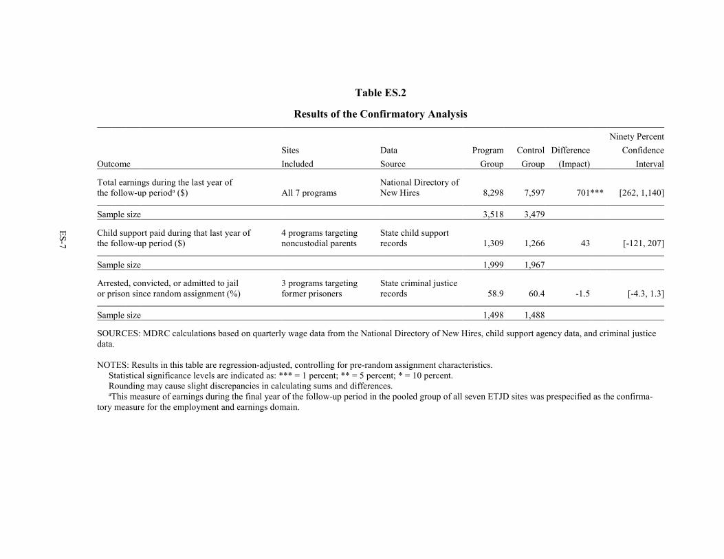
Table ES.2
Results of the Confirmatory Analysis
Ninety Percent Sites Data Program Control Difference Confidence
Outcome Included Source Group Group (Impact) Interval
Total earnings during the last year of the follow-up perioda ($) All 7 programs
National Directory of New Hires 8,298 7,597 701 *** [262, 1,140]
Sample size 3,518 3,479
Child support paid during that last year of the follow-up period ($)
4 programs targeting noncustodial parents
State child support records 1,309 1,266 43 [-121, 207]
Sample size 1,999 1,967
Arrested, convicted, or admitted to jail or prison since random assignment (%)
3 programs targeting former prisoners
State criminal justice records 58.9 60.4 -1.5 [-4.3, 1.3]
Sample size 1,498 1,488
SOURCES: MDRC calculations based on quarterly wage data from the National Directory of New Hires, child support agency data, and criminal justice data.
NOTES: Results in this table are regression-adjusted, controlling for pre-random assignment characteristics. Statistical significance levels are indicated as: *** = 1 percent; ** = 5 percent; * = 10 percent. Rounding may cause slight discrepancies in calculating sums and differences. aThis measure of earnings during the final year of the follow-up period in the pooled group of all seven ETJD sites was prespecified as the confirma-tory measure for the employment and earnings domain.
ES-7
ES-8
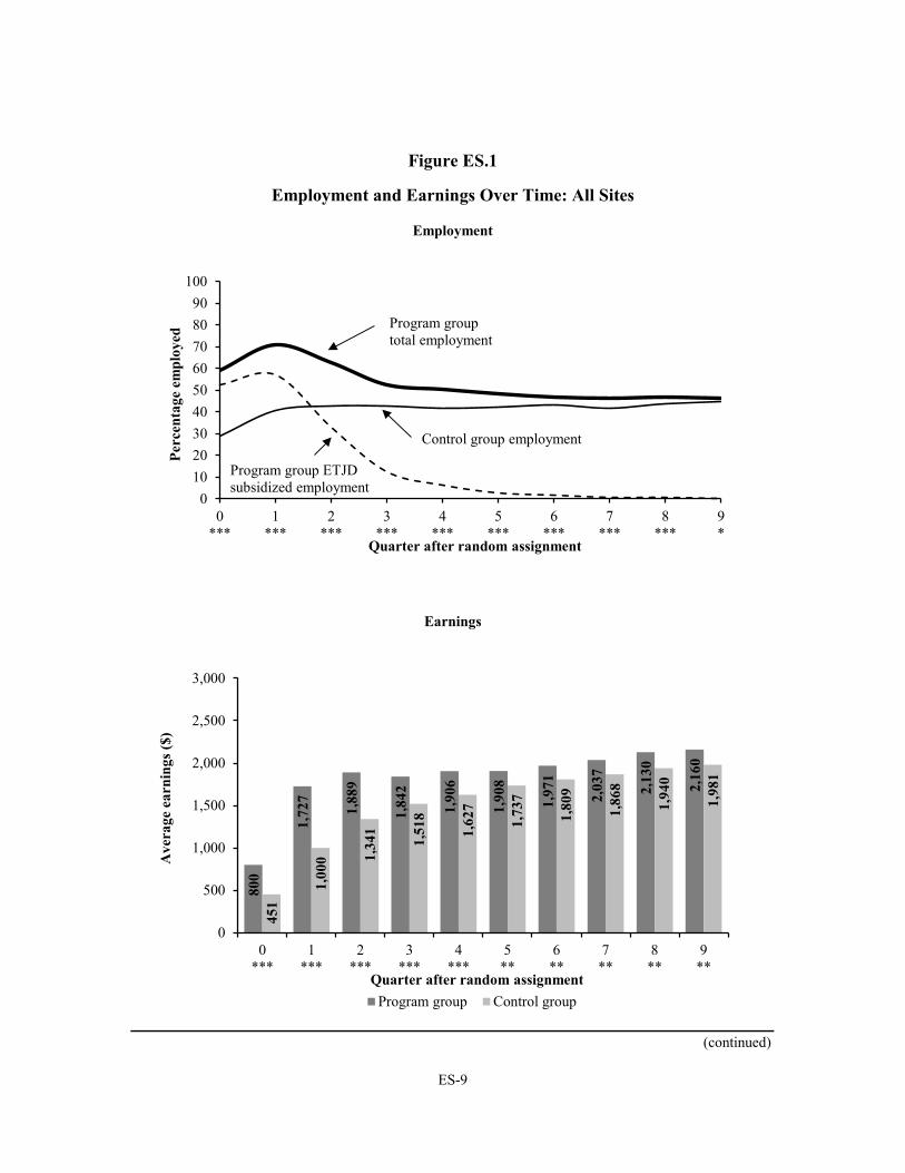
earnings impact is larger than the average long-term earnings impacts from several other recent studies of employment and training programs for hard-to-employ job seekers.12 The bottom panel of Figure ES.1 shows that the programs increased earnings by as much as 73 percent in the early quarters of the study period, when many program group members were working in transitional jobs. The earnings impacts grew much smaller over time but remained statistically significant throughout the 30-month follow-up period. Exploratory analyses discussed below provide further evidence to support this confirmatory finding.
Table ES.2 also shows that at the four sites targeting noncustodial parents, there was no statistically significant difference in the amount of child support paid, on average, by members of the program and control groups in the last year of the follow-up period. The table also shows that at the three sites targeting people recently released from prison, a similar proportion of people in the program and control groups were arrested, convicted of a crime, or incarcerated during the 30-month follow-up period.
Impact Findings: Exploratory Analysis
The confirmatory analysis presented in the previous section is the most definitive evi-dence on the impact of ETJD. The evaluation team also conducted exploratory analyses of a somewhat larger group of outcome measures in the same three domains, in order to provide a more nuanced picture of the results and to identify possible strengths programs could build on and weaknesses to be corrected. The findings from the exploratory analysis are less definitive because a larger number of outcomes were examined, raising the odds that statistically significant impacts may have arisen by chance.13 The team examined three broad topics in the exploratory analysis: (1) impacts on other measures in the three primary outcome domains; (2) impacts among subgroups of the ETJD population; and (3) impacts for the individual ETJD programs. Findings from the exploratory analysis include:
12In a recent literature review conducted for the U.S. Health and Human Services Office of Planning, Re-search, and Evaluation, only 3 of 23 studies published between 2010 and 2014 about employment and training programs targeting hard-to-employ job seekers demonstrated positive impacts on long-term earnings (defined as earnings more than 18 months after study entry). Studies of programs involving primarily conditional cash trans-fer, parenting, or health interventions were not included in this tally, nor were programs targeting already-em-ployed individuals. See the Employment Strategies for Low-Income Adults Evidence Review, available at https://employmentstrategies.acf.hhs.gov.
13Increasing the number of impact estimates examined increases the likelihood that at least one estimate will be statistically significant by chance, even if the program had no true effect. If 10 independent outcomes are examined, for example, it is likely that one of them will show an effect that is statistically significant at the 10 percent level purely by chance, even if the program is truly ineffective.
ES-9
(continued)
Figure ES.1
Employment and Earnings Over Time: All Sites
Employment
Earnings
800
1,72
7
1,88
9
1,84
2
1,90
6
1,90
8
1,97
1
2,03
7
2,13
0
2,16
0
451
1,00
0 1,34
1
1,51
8
1,62
7
1,73
7
1,80
9
1,86
8
1,94
0
1,98
1
0
500
1,000
1,500
2,000
2,500
3,000
0***
1***
2***
3***
4***
5**
6**
7**
8**
9**
Ave
rage
ear
ning
s ($)
Quarter after random assignmentProgram group Control group
0102030405060708090
100
0***
1***
2***
3***
4***
5***
6***
7***
8***
9*
Perc
enta
ge e
mpl
oyed
Quarter after random assignment
Program group total employment
Control group employment
Program group ETJD subsidized employment

ES-10
•
•
Figure ES.1 (continued)
SOURCES: MDRC calculations based on quarterly wage data from the National Directory of New Hiresand program payroll records.
NOTES: Results in this table are regression-adjusted, controlling for pre-random assignment characteristics.
Statistical significance levels are indicated as: *** = 1 percent; ** = 5 percent; * = 10 percent.Employment rates and earnings in the quarter of random assignment through Quarter 5 after random
assignment include both ETJD subsidized jobs and jobs covered by unemployment insurance and reported to the National Directory of New Hires. Employment rates and earnings in Quarters 6 through 9 after random assignment include only jobs covered by unemployment insurance and reported to the National Directory of New Hires.
In addition to having higher total earnings than the control group in the last year of the follow-up period, the program group was also somewhat more likely to be employed, and to be working in higher-quality jobs.
Table ES.3 shows some of the important outcomes that were examined in the exploratory analysis in each of the primary domains. The top panel of the table shows that about 60 percent of the control group worked in a job covered by unemployment insurance in the last year of the follow-up period. The program group’s employment rate was about 64 percent, and the 4 per-centage point difference between the program and control group is statistically significant. Re-sponses to the 30-month survey tell a similar story, though the survey found higher employment rates for both groups (probably because some respondents were working in jobs not covered by unemployment insurance). The survey also shows that after 30 months, the program group was more likely to be working in full-time jobs, jobs that paid more than $10 an hour, and jobs that were permanent rather than temporary. Another analysis (not shown) found that the program group was somewhat more likely to have employer-provided health insurance.
Although the ETJD programs targeting noncustodial parents did not sig-nificantly increase the amount of formal child support paid in the last year of the follow-up period, program group members at those sites were somewhat more likely to pay at least some formal support during the year.
It may seem surprising that ETJD increased earnings without increasing the amount of child support paid, since child support is generally deducted from workers’ paychecks. This pat-tern suggests that program group members paid a slightly lower percentage of their earnings for child support than control group members. As shown in the middle panel of Table ES.3, the
ES-11
Table ES.3
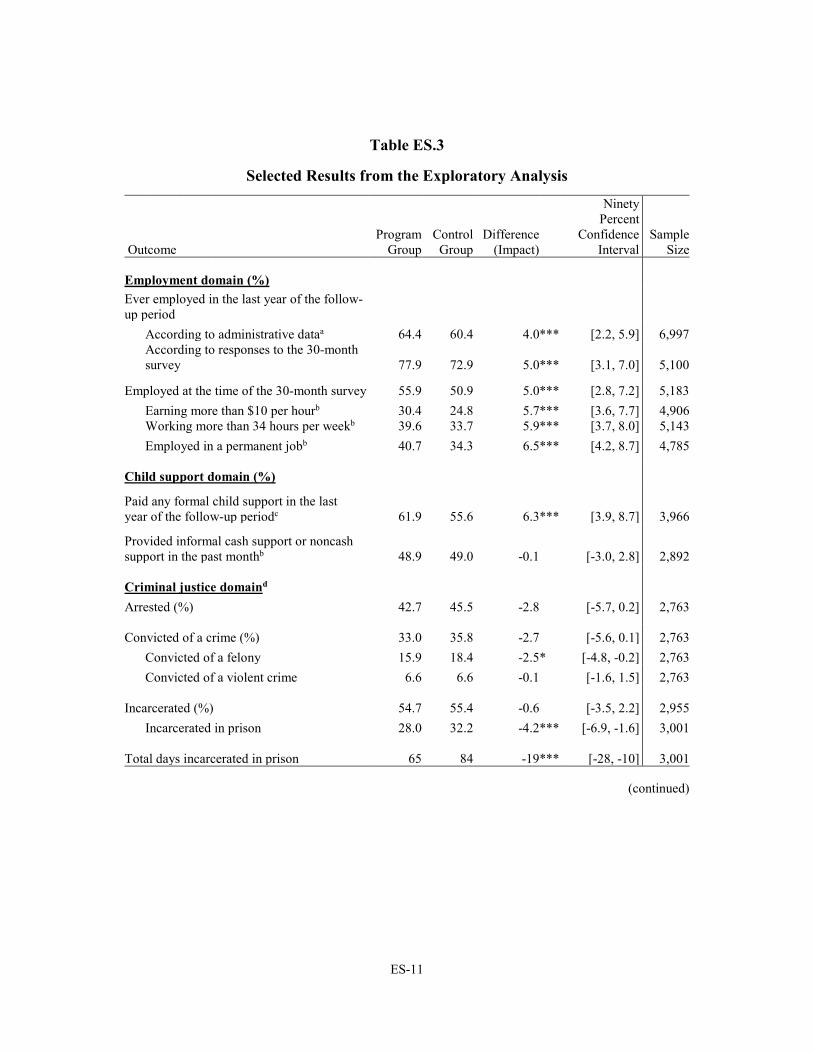
(continued)
Selected Results from the Exploratory Analysis
Outcome Program
Group Control
Group Difference
(Impact)
Ninety Percent
Confidence Interval
Sample Size
Employment domain (%) Ever employed in the last year of the follow-up period
According to administrative dataa 64.4 60.4 4.0 *** [2.2, 5.9] 6,997 According to responses to the 30-month survey 77.9 72.9 5.0 *** [3.1, 7.0] 5,100
Employed at the time of the 30-month survey 55.9 50.9 5.0 *** [2.8, 7.2] 5,183 Earning more than $10 per hourb 30.4 24.8 5.7 *** [3.6, 7.7] 4,906 Working more than 34 hours per weekb 39.6 33.7 5.9 *** [3.7, 8.0] 5,143 Employed in a permanent jobb 40.7 34.3 6.5 *** [4.2, 8.7] 4,785
Child support domain (%)
Paid any formal child support in the last year of the follow-up periodc 61.9 55.6 6.3 *** [3.9, 8.7] 3,966
Provided informal cash support or noncash support in the past monthb 48.9 49.0 -0.1 [-3.0, 2.8] 2,892
dCriminal justice domain Arrested (%) 42.7 45.5 -2.8 [-5.7, 0.2] 2,763
Convicted of a crime (%) 33.0 35.8 -2.7 [-5.6, 0.1] 2,763 Convicted of a felony 15.9 18.4 -2.5 * [-4.8, -0.2] 2,763 Convicted of a violent crime 6.6 6.6 -0.1 [-1.6, 1.5] 2,763
Incarcerated (%) 54.7 55.4 -0.6 [-3.5, 2.2] 2,955 Incarcerated in prison 28.0 32.2 -4.2 *** [-6.9, -1.6] 3,001
Total days incarcerated in prison 65 84 -19 *** [-28, -10] 3,001

ES-12
Table ES.3 (continued) SOURCES: MDRC calculations based on quarterly wage data from the National Directory of New Hires, child sup-port agency data, criminal justice data, and responses to the ETJD 30-month survey. NOTES: Results in this table are regression-adjusted, controlling for pre-random assignment characteristics. Anal-yses of survey-based outcomes incorporate weights that correct for survey nonresponse, which take into considera-tion information on the full sample’s pre-random assignment characteristics. Unweighted analyses (not shown) yielded nearly identical results. Statistical significance levels are indicated as: *** = 1 percent; ** = 5 percent; * = 10 percent. Rounding may cause slight discrepancies in calculating sums and differences. aEmployment rates include only jobs covered by unemployment insurance and reported to the National Directory of New Hires. bMeasure created from responses to the ETJD 30-month survey. cMeasures of formal child support include all payments made through the state's child support collection and dis-bursement unit, including funds from employer withholding and other sources (for example, tax intercepts). dAll criminal justice measures are created from state criminal justice data sources.
program group was somewhat more likely to pay formal child support in the last year of the follow-up period, which is consistent with the impact on employment discussed in the previous section.14 This finding means that program group members who paid support paid slightly less than control group payers. There may be lags in the child support system’s ability to begin col-lecting support once an individual finds a job. In addition, in one of the programs, participants’ child support orders were routinely lowered as an incentive to participate in ETJD; the orders may not have been immediately increased when participants got unsubsidized jobs.
• While the ETJD programs targeting formerly incarcerated people did not significantly reduce the number of people who had at least one criminal justice “event” during the follow-up period, there is some evidence that the programs affected other measures of recidivism.
The bottom panel of Table ES.3 shows that program group members in the three pro-grams targeting recently released people were less likely to have been convicted of a felony or to have been incarcerated in prison during the follow-up period, and spent fewer days in prison overall than the control group. These impacts are generally small but statistically significant. As discussed further below, the impacts on recidivism outcomes overall mostly reflect the impacts in Indianapolis.
14The middle panel of Table ES.3 shows results for the four programs targeting noncustodial parents. In
those programs, the program group earned about $1,000 more than the control group in the last year of the follow-up period, a statistically significant difference. Sixty-eight percent of the program group at those sites worked in the last year, compared with 63 percent of the control group, a difference that is also statistically significant.
ES-13
While the majority of sample members had some contact with the criminal justice system during the follow-up period, few were convicted of a serious new crime (that is, a felony or a violent crime).
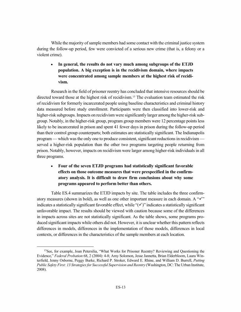
• In general, the results do not vary much among subgroups of the ETJDpopulation. A big exception is in the recidivism domain, where impactswere concentrated among sample members at the highest risk of recidi-vism.
Research in the field of prisoner reentry has concluded that intensive resources should be directed toward those at the highest risk of recidivism.15 The evaluation team estimated the risk of recidivism for formerly incarcerated people using baseline characteristics and criminal history data measured before study enrollment. Participants were then classified into lower-risk and higher-risk subgroups. Impacts on recidivism were significantly larger among the higher-risk sub-group. Notably, in the higher-risk group, program group members were 12 percentage points less likely to be incarcerated in prison and spent 41 fewer days in prison during the follow-up period than their control group counterparts; both estimates are statistically significant. The Indianapolis program — which was the only one to produce consistent, significant reductions in recidivism — served a higher-risk population than the other two programs targeting people returning from prison. Notably, however, impacts on recidivism were larger among higher-risk individuals in all three programs.
• Four of the seven ETJD programs had statistically significant favorableeffects on those outcome measures that were prespecified in the confirm-atory analysis. It is difficult to draw firm conclusions about why someprograms appeared to perform better than others.
Table ES.4 summarizes the ETJD impacts by site. The table includes the three confirm-atory measures (shown in bold), as well as one other important measure in each domain. A “” indicates a statistically significant favorable effect, while “()” indicates a statistically significant unfavorable impact. The results should be viewed with caution because some of the differences in impacts across sites are not statistically significant. As the table shows, some programs pro-duced significant impacts while others did not. However, it is unclear whether this pattern reflects differences in models, differences in the implementation of those models, differences in local contexts, or differences in the characteristics of the sample members at each location.
15See, for example, Joan Petersilia, “What Works for Prisoner Reentry? Reviewing and Questioning the Evidence,” Federal Probation 68, 2 (2004): 4-8; Amy Solomon, Jesse Jannetta, Brian Elderbloom, Laura Win-terfield, Jenny Osborne, Peggy Burke, Richard P. Stroker, Edward E. Rhine, and William D. Burrell, Putting Public Safety First: 13 Strategies for Successful Supervision and Reentry (Washington, DC: The Urban Institute, 2008).
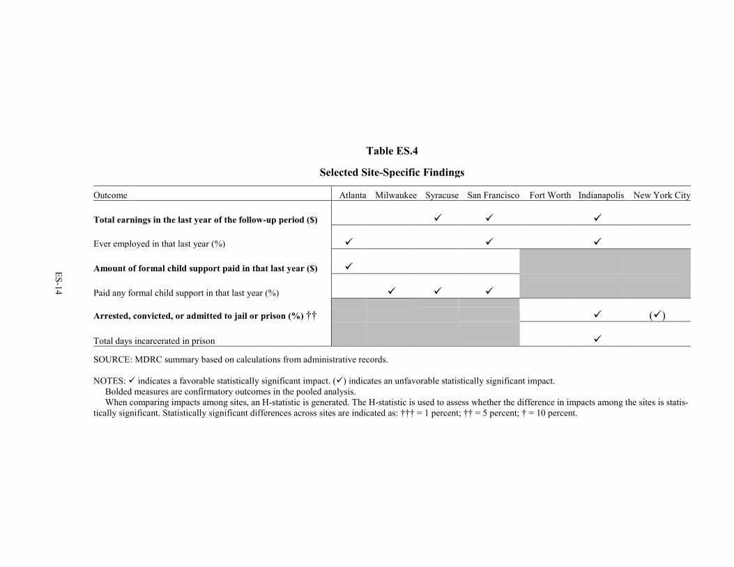
Table ES.4
Selected Site-Specific Findings
Outcome Atlanta Milwaukee Syracuse San Francisco Fort Worth Indianapolis New York City
Total earnings in the last year of the follow-up period ($)
Ever employed in that last year (%)
Amount of formal child support paid in that last year ($)
Paid any formal child support in that last year (%)
Arrested, convicted, or admitted to jail or prison (%) †† ()
Total days incarcerated in prison
SOURCE: MDRC summary based on calculations from administrative records.
NOTES: indicates a favorable statistically significant impact. () indicates an unfavorable statistically significant impact. Bolded measures are confirmatory outcomes in the pooled analysis. When comparing impacts among sites, an H-statistic is generated. The H-statistic is used to assess whether the difference in impacts among the sites is statis-tically significant. Statistically significant differences across sites are indicated as: ††† = 1 percent; †† = 5 percent; † = 10 percent.
ES-14

ES-15
Major observations include:
•
•
•
•
•
The Indianapolis program produced substantial impacts in both the employ-ment and recidivism domains. Control group data indicate that the program served a very disadvantaged population with poor employment outcomes and high rates of recidivism. The program used an intensive, highly supportive model in which participants were often supervised by peers who were program graduates in an electronics recycling social enterprise (a business with a social purpose). A companion report describes the results of a full benefit-cost study focusing on this program.16
The San Francisco program produced substantial impacts in both the employ-ment and child support domains. This result is somewhat surprising, because the program’s three-tiered transitional jobs model did not operate as planned and fewer than half of the program group members worked in subsidized jobs. However, there was strong collaboration with the local child support agency, which routinely lowered program group members’ monthly child support or-ders to provide an incentive for participation.
The Atlanta program produced modest impacts on employment and child sup-port payments. Based on control group outcomes, the Atlanta program served the most employable population of any in the ETJD project. Its staged model was generally well implemented and the rate of participation in transitional jobs was close to 100 percent.
The Syracuse program produced modest impacts in the employment and child support domains. Its transitional jobs model was fairly traditional, with only modest enhancements, and was generally well implemented. The program served a highly disadvantaged population.
The Milwaukee program produced few significant impacts. The program ex-perienced implementation challenges: there was staff turnover and an initial plan to place a large proportion of ETJD participants into occupational training was not implemented. The model included an innovative earnings supplement, but it did not apply to many people in practice. In addition, a large proportion of the control group reported receiving employment services, which may have made it more difficult for the program to achieve significant impacts.
16Foley, Farrell, Webster, and Walter (forthcoming).
ES-16
•
•
Fort Worth did not have significant impacts in either the employment or the recidivism domain. This program was the only one in the project that at-tempted to place almost all participants into transitional jobs with private em-ployers. Perhaps as a result of this approach, fewer than 40 percent of partici-pants worked in transitional jobs. Other programs that have attempted to place disadvantaged people into subsidized jobs in the private sector have seen very similar placement rates.17
The New York City program did not produce favorable significant impacts. As noted earlier, a large proportion of the control group received employment services and, in addition, the research team was able to determine that a sub-stantial proportion of the control group (about 36 percent) received transitional jobs through another large transitional jobs program in the city (while about 16 percent of the program group also received transitional jobs through that other program). The program’s unfavorable impact on overall recidivism re-flects increases in arrests and jail incarceration. These results are puzzling, par-ticularly because the program significantly reduced felony convictions and ad-missions to prison for new crimes.
Conclusion The ETJD project set out to test whether “enhanced” transitional jobs programs could produce larger impacts than earlier models after participants moved on. The answer is a qualified “yes.” As a group, the ETJD programs produced a modest but statistically significant increase in earn-ings in the last year of the follow-up period, a result that was not found in most earlier studies.18 Exploratory analyses suggest that the programs probably produced a number of other modest but positive effects on outcomes in all three primary domains. Thus, it seems clear that transitional jobs programs can produce effects in the employment, child support, and criminal justice domains after participants leave the program. That said, the impacts after participants left the programs were not large. Moreover, it is not clear whether transitional jobs are more cost-effective than other approaches with the same goal.
17See, for example, Asaph Glosser, Bret Barden, and Sonya Williams, Testing Two Subsidized Employment Approaches for Recipients of Temporary Assistance for Needy Families: Implementation and Early Impacts of the Los Angeles County Transitional Subsidized Employment Program, OPRE Report 2016-77 (Washington, DC: Office of Planning, Research and Evaluation, Administration for Children and Families, U.S. Department of Health and Human Services, 2016).
18It is important to note that the pooled ETJD sample (about 7,000) is substantially larger than the samples in most earlier evaluations of transitional jobs programs. It is not clear whether an impact on earnings of the size measured in ETJD (about $700 in the last year of the follow-up period) would have been statistically significant with a smaller sample.
ES-17
It is also difficult to draw firm conclusions about the factors that are associated with these longer-term positive earnings, child support, and criminal justice effects. The ETJD programs that appear to have been most effective served different populations, used different models, and had different levels of implementation success. And there does not appear to be a correlation between the extent of “enhancement” and the level of impact.
Finally, it is important to note that, despite the positive impacts, most sample members in both the program and control groups were still struggling in the labor market at the end of the study’s follow-up period. For example, only about one-third of those who responded to the 30-month survey reported having full-time jobs (working more than 34 hours per week). Individuals in the ETJD target groups would probably need to develop substantially greater skills in order to obtain better-paying, more stable jobs. Recent studies have shown that certain kinds of occupa-tional training programs can produce such gains, but it is not clear that ETJD participants could qualify for such programs or support themselves while participating.19 It may be that models com-bining subsidized employment and skills training could achieve better results.
From a policy perspective, ETJD confirmed once again that transitional jobs programs, if properly targeted and executed, will produce very large short-term increases in employment and earnings. Some of the additional earnings of noncustodial parents will find their way to chil-dren. Other research (partly based on 12-month results from two ETJD sites) suggests that these gains can translate into parallel improvements in personal well-being.20
Policymakers will need to decide whether these nearly certain short-term effects — cou-pled with the possibility of longer-term impacts such as those found in ETJD — are sufficient to justify additional investment. The answer depends, in part, on how one views the goals of these programs. If the main objective is to find the most cost-effective strategy for improving long-term employment outcomes for disadvantaged workers, transitional jobs may not be superior to other approaches. On the other hand, if a major goal is to provide meaningful work and income to people who cannot find jobs in the regular labor market, transitional jobs and other types of subsidized employment may be seen as good investments; the possibility of longer-term gains and reductions
19See, for example, Richard Hendra, David H. Greenberg, Gayle Hamilton, Ari Oppenheim, Alexandra Pennington, Kelsey Schaberg, and Betsy L. Tessler, Encouraging Evidence on a Sector-Focused Advancement Strategy: Two-Year Impacts from the WorkAdvance Demonstration (New York: MDRC, 2016).
20Two of the ETJD sites (Atlanta and San Francisco) were also part of the parallel Subsidized and Transi-tional Employment Demonstration (STED), sponsored by the Administration for Children and Families in the U.S. Department of Health and Human Services. The STED project administered a brief survey to program and control group members just a few months after random assignment, when many program group members were working in transitional jobs, in order to measure some of the ancillary benefits of employment. See Sonya Wil-liams and Richard Hendra, The Effects of Subsidized and Transitional Employment Programs on Noneconomic Well-Being, OPRE Report 2018-17 (Washington, DC: Office of Planning, Research, and Evaluation, Admin-istration for Children and Families, U.S. Department of Health and Human Resources, 2018).

ES-18
in recidivism may be viewed as a bonus. Such programs are broadly applicable when overall economic conditions are poor, but subsidized employment programs targeting particular pop-ulations or geographic areas may make sense even when the overall unemployment rate is low.
1
Chapter 1
Introduction
Across the United States, some adults have great difficulty finding and holding jobs even when overall economic conditions are good. These individuals typically have low levels of formal ed-ucation and skills and other characteristics such as criminal records that place them at the back of the queue for job openings.
Many programs have been developed to assist hard-to-employ job seekers, but few have demonstrated sustained success.1 One model that has been implemented and tested fairly exten-sively is called “transitional jobs.” Transitional jobs programs offer temporary jobs, subsidized with public funds, that aim to teach participants basic work skills or help them get a foot in the door with an employer. Many programs also offer assistance with personal issues that may hinder participants’ success, and help participants find permanent jobs.
This report presents final results from the Enhanced Transitional Jobs Demonstration (ETJD), which used a rigorous random assignment research design to evaluate seven transitional jobs programs targeting either individuals who had recently been released from prison, or parents who did not have custody of their children (“noncustodial” parents), who owed child support, and who were unable to meet their obligations because they were unemployed. The ETJD programs were designed to try to address limitations identified by previous evaluations of transitional jobs programs, which are described further below. The ETJD project was conceived and funded by the Employment and Training Administration in the U.S. Department of Labor (DOL). The eval-uation is also supported by the Administration for Children and Families (ACF), part of the U.S. Department of Health and Human Services.2 MDRC is leading the project under contract to DOL along with two partners: Abt Associates and MEF Associates.3
1For examples of such programs, see the U.S. Department of Health and Human Services Office of Plan-ning, Research, and Evaluation’s “Employment Strategies for Low-Income Adults Evidence Review,” a system-atic review of the literature on the effect of employment and training programs and strategies for low-income individuals, available at https://employmentstrategies.acf.hhs.gov.
2The ACF-funded Subsidized and Transitional Employment Demonstration (STED) is also testing subsi-dized employment programs for low-income populations. Because the noncustodial parent population was of special interest to ACF, two of the ETJD programs (those in Atlanta and San Francisco) were included in both projects.
3A separate organization, Coffey Consulting, received a contract to provide technical assistance to the ETJD grantees.

2
The report examines the impacts of the ETJD programs in the 30-month period after par-ticipants entered the study, as well as the costs of the programs. It builds on an earlier report that presented detailed implementation findings and impacts after 12 months.4
Background and Context The roots of the ETJD project can be traced to two broad policy trends. The first is the ongoing struggle to find effective models to assist people who have great difficulty finding or keeping jobs, regardless of overall labor market conditions. Policymakers tend to focus on these individ-uals when they incur public costs — for example, by receiving public assistance, by failing to pay child support (which may, in turn, lead to higher public-assistance costs for their children), or by committing crimes and ending up in jail or prison.
The transitional jobs model has long been considered a promising approach for the hard-to-employ. However, rigorous evaluations of transitional jobs programs have identified limita-tions of the model. On the one hand, most of the programs that were tested dramatically increased participants’ employment rates initially, suggesting that the programs provided jobs and income to many people who would otherwise have been unemployed.5 On the other hand, in most cases, the gains in employment were the result of the subsidized jobs, and they faded when the jobs ended. Five of the programs that were previously evaluated targeted individuals who had recently been released from prison, but only one of them led to sustained reductions in recidivism — the rate at which former prisoners commit new crimes or are reincarcerated.6 While many policy-makers and practitioners continue to see transitional jobs as promising, these results highlight the need to identify new variations of the model that produce longer-lasting impacts. With the passage of the Workforce Innovation and Opportunity Act in 2014, transitional jobs became an allowable work-based training activity within the public workforce system, expanding the possibility of using transitional jobs to help low-income people move into the workforce.7
The second policy trend is the evolution of the corrections and child support-enforcement systems in recent years. Both of these systems have long viewed their missions in narrow terms: The corrections system sought to punish and segregate people who had been convicted of crimes, and the child support system sought to establish and enforce child support orders. However, in recent years, both systems have begun to focus more on improving the outcomes of their “clients.”
4Redcross et al. (2016). 5For a recent summary of evaluations of transitional jobs programs and other subsidized employment mod-
els, see Dutta-Gupta, Grant, Eckel, and Edelman (2016). 6See, for example, Valentine (2012); Redcross, Millenky, Rudd, and Levshin (2012); and Butler et al.
(2012). 7See U.S. Department of Labor, Employment and Training Administration (2015).
3
Criminal justice agencies increasingly provide reentry support to the more than 600,000 people who are released from prison each year,8 and more child support agencies are providing or ar-ranging for services for noncustodial parents who are unable to meet their obligations. Transi-tional jobs programs are seen as a potentially effective approach for these populations, in part because they provide immediate income while participants are learning work skills. Policymakers hope that additional income and the acquisition of employment-related skills will reduce partici-pants’ propensity to engage in criminal activity and increase their likelihood of making child sup-port payments.
The ETJD Project and the Evaluation In 2011, DOL held a national competition to select programs to participate in the ETJD project. Applicants were required to describe specific “enhancements” to the basic transitional jobs model that had been tested earlier and to explain why they believed their approaches would achieve better results than previous programs. In addition, applicants were required to identify a primary target group — either individuals released from prison in the previous 120 days or noncustodial parents who owed child support but were unable to pay because they were unemployed. Ulti-mately, DOL selected seven programs — four targeting noncustodial parents and three targeting people recently released from prison — and provided each one with approximately $6 million over a period of four years.9
The evaluation was shaped by the broader objectives of the demonstration. Subsidized employment programs have different goals. Some programs — typically those operated during economic downturns — are designed primarily to provide work-based income support to jobless workers. Such programs might be assessed on their ability to expand quickly to a large scale and provide useful jobs. Other models also provide income, but their primary goal is to use subsidized jobs as a tool to help hard-to-employ individuals “learn to work by working” in order to improve their ability to get and hold unsubsidized jobs. The ETJD programs fall into the second category. DOL therefore sought to assess their effectiveness in large part based on how participants fared in the labor market after leaving the subsidized jobs. Because the ETJD programs targeted non-custodial parents and recently incarcerated individuals, they also aimed to increase the payment of child support and reduce recidivism, outcomes that may be tied to employment. Overall, the evaluation set out to answer three broad research questions:
● How were the ETJD programs designed and operated, and whom did they serve?
8Carson and Sabol (2012). 9For more information about the grant requirements, see U.S. Department of Labor, Employment and Train-
ing Administration (2011).
4
●
●
How did the ETJD programs affect participants’ receipt of services and their outcomes in three primary domains: employment, child support, and criminal justice?
How did the programs’ costs compare with any benefits they produced?
The first and third questions were addressed by the evaluation’s implementation and cost-effectiveness/cost-benefit studies.10 The second question was addressed by the impact study, which used a random assignment research design, the most reliable method for assessing the ef-fectiveness of this type of program.
To facilitate the evaluation, each ETJD program was required to recruit 1,000 people who wanted to participate in the program, who met the eligibility requirements, and who agreed to participate in the study. These individuals were randomly assigned either to the program group, whose members were invited to participate in the ETJD program, or to the control group, whose members were usually given a list of other services in the community.11 (In some places, the control group was referred to a specific program that provided job-search assistance but not tran-sitional jobs.) The MDRC team followed the program and control groups for two and a half years (30 months) using surveys and federal, state, and local administrative records to measure out-comes in the three primary domains — employment, criminal justice, and child support — as well as in other, secondary areas, such as family engagement.12 If differences emerge between the groups over time and these differences are large enough to reach conventional levels of statistical significance, then one can be fairly confident that the differences are attributable to the ETJD program. Such differences are referred to as “impact estimates.” This report presents impact esti-mates for four overlapping groups of ETJD programs: (1) the pooled group of all seven ETJD programs; (2) the pooled group of four programs specifically targeting noncustodial parents; (3) the pooled group of three programs specifically targeting formerly incarcerated people; and (4) each program separately.
10This report includes results from the cost-effectiveness study. An upcoming document presents results from a full benefit-cost study of one of the ETJD programs. See Foley, Farrell, Webster, and Walter (forthcom-ing).
11As shown in Appendix I, there were no systematic differences in baseline characteristics between program and control group members.
12Administrative records are data used for the management of programs and public services. Administrative records used for analyses in this report include quarterly wage records from the National Directory of New Hires, child support records from state child support agencies, jail records from local county or city jails, and arrest, conviction, and prison records from state criminal justice agencies. Surveys included 12-month and 30-month surveys administered at all of the experimental sites (“site” being a term that encompasses the program, the program group, the control group, and the local environment), and an earlier survey administered at two of the sites. See Chapter 1 of the interim report for more detailed information on the data sources used in the project.
5
To ensure the most rigorous interpretation and presentation of evidence, this report di-vides findings into two categories: confirmatory findings provide conclusive evidence of a pro-gram’s impact, while exploratory findings provide suggestive evidence. These two categories of findings are defined and explained in Box 1.1. In brief, three confirmatory measures were established for the project, one in each of the three primary domains that the ETJD intervention was designed to affect (employment, criminal justice, and child support). All confirmatory measures were derived from administrative data, as these sources were viewed as the most con-sistently reliable sources of information.13 The confirmatory measures are:
●
●
●
In the employment domain, earnings in the final year of the follow-up pe-riod, which begins during the sixth quarter after a person entered the study and concludes at the end of the ninth quarter (or approximately 1.5 to 2.5 years after the person entered the study). This measure covers a period after nearly all program group members had left subsidized jobs. The earnings outcome reflects several components of labor-market success: whether people were em-ployed, how consistently they were employed, and the wages they received. Because all ETJD programs were designed to increase participants’ earnings, this measure is assessed for all seven ETJD programs, pooled together.
In the child support domain, the total amount of child support paid in the final year of the follow-up period. Since child support payments are typically deducted from parents’ paychecks, this measure covers the same span of time as the earnings measure and assesses the payment of child support after pro-gram group members were no longer in subsidized jobs. This measure was assessed for all participants in the four programs targeting noncustodial par-ents, pooled together.
In the criminal justice domain, any criminal justice event (an arrest, convic-tion, or admission to jail or prison) during the entire 30-month follow-up pe-riod after random assignment. This measure was assessed for all participants in the three ETJD programs targeting formerly incarcerated people, pooled to-gether.
13Administrative records are considered more reliable as they are available for all sample members, not just those who responded to ETJD surveys. Further, the final ETJD survey was administered around 30 months after random assignment and in some cases captures only point-in-time measures at the time of the survey, or measures that happened up until the time of the survey. In contrast, administrative records have more comprehensive data available for important outcomes (earnings, child support payments, and criminal justice events) over time and at specific points in time. Administrative data are also not subject to errors in memory or intentional misreporting.
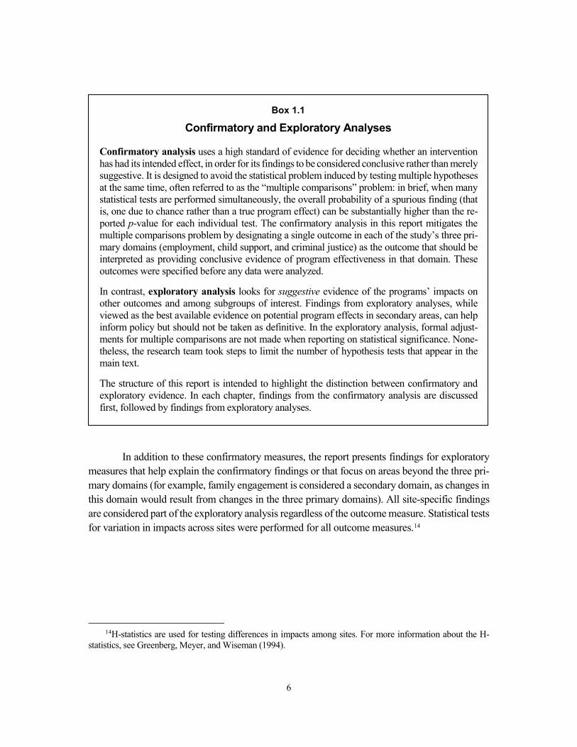
6
Box 1.1
Confirmatory and Exploratory Analyses
Confirmatory analysis uses a high standard of evidence for deciding whether an intervention has had its intended effect, in order for its findings to be considered conclusive rather than merely suggestive. It is designed to avoid the statistical problem induced by testing multiple hypotheses at the same time, often referred to as the “multiple comparisons” problem: in brief, when many statistical tests are performed simultaneously, the overall probability of a spurious finding (that is, one due to chance rather than a true program effect) can be substantially higher than the re-ported p-value for each individual test. The confirmatory analysis in this report mitigates the multiple comparisons problem by designating a single outcome in each of the study’s three pri-mary domains (employment, child support, and criminal justice) as the outcome that should be interpreted as providing conclusive evidence of program effectiveness in that domain. These outcomes were specified before any data were analyzed.
In contrast, exploratory analysis looks for suggestive evidence of the programs’ impacts on other outcomes and among subgroups of interest. Findings from exploratory analyses, while viewed as the best available evidence on potential program effects in secondary areas, can help inform policy but should not be taken as definitive. In the exploratory analysis, formal adjust-ments for multiple comparisons are not made when reporting on statistical significance. None-theless, the research team took steps to limit the number of hypothesis tests that appear in the main text.
The structure of this report is intended to highlight the distinction between confirmatory and exploratory evidence. In each chapter, findings from the confirmatory analysis are discussed first, followed by findings from exploratory analyses.
In addition to these confirmatory measures, the report presents findings for exploratory measures that help explain the confirmatory findings or that focus on areas beyond the three pri-mary domains (for example, family engagement is considered a secondary domain, as changes in this domain would result from changes in the three primary domains). All site-specific findings are considered part of the exploratory analysis regardless of the outcome measure. Statistical tests for variation in impacts across sites were performed for all outcome measures.14
14H-statistics are used for testing differences in impacts among sites. For more information about the H-statistics, see Greenberg, Meyer, and Wiseman (1994).
7
The ETJD Programs Table 1.1 briefly describes the seven ETJD programs. Most of the grantees were private, nonprofit organizations, though, as described later, these organizations worked very closely with state or local government partners.
Each of the seven programs was designed somewhat differently but, as required by DOL, all of them were enhanced in some ways relative to the transitional jobs models that were studied earlier. Those earlier programs mostly provided temporary subsidized jobs either within the pro-gram itself or with other nonprofit organizations. They also assigned participants to job coaches or case managers who helped them address barriers to employment and, in some cases, to job developers who helped them search for unsubsidized jobs.15 As displayed in Table 1.2, the ETJD enhancements fell into three general categories:
●
●
●
Structural changes. The programs that were tested in earlier studies placed participants into relatively sheltered positions with a program operator or a partner organization, and then helped them find regular jobs. Two of the ETJD programs used “staged” models in which participants started in program jobs, but then progressed to subsidized jobs in the community that more closely re-sembled “real” jobs. A third program focused entirely on placing participants directly into subsidized jobs in the private sector that were intended to evolve into permanent positions. A fourth used a “tiered” model that placed partici-pants into different types of subsidized jobs based on their educational and work histories. For the most part, these new structural approaches were de-signed to promote smoother transitions from subsidized to unsubsidized jobs.
Enhanced support. Four of the ETJD programs aimed to provide special sup-port or assistance that was not available in the earlier programs studied — for example, opportunities for short-term training in occupational skills, services to help participants address problematic behavior patterns, or help correcting errors in their official criminal records.
Child support incentives. In two of the four programs targeting noncustodial parents, the child support agency offered special “carrots,” “sticks,” or both to encourage participants to remain active in the ETJD program. For example, in one program, program group members’ child support orders were modified
15Job developers established relationships with employers and provided final employment preparation (in interview skills, self-presentation, and job-search strategies) to connect participants with positions and follow up on applications.

8
Table 1.1
ETJD Individual Program Characteristics
Location, Program Opera-tor, and Name
Target Group Program Overview
Atlanta, GA Goodwill of North Georgia Good Transitions
Noncustodial parents
Participants worked at a Goodwill store for approximately one month, then moved into a less supported subsidized position with a private employer in the community for about three months. The program offered case management and short-term training.
Milwaukee, WI YWCA of Southeast Wisconsin Supporting Families Through Work
Noncustodial parents
Participants started in a three- to five-day job-readiness workshop. They were then placed in transitional jobs, mostly with private-sec-tor employers. The program supplemented wages in unsubsidized employment to bring them up to $10 an hour for six months. The program also provided child support-related assistance.
San Francisco, CA Goodwill Industries, with San Francisco Dept. of Child Support Services TransitionsSF
Noncustodial parents
Participants began with an assessment followed by two weeks of job-readiness training. Then they were placed into one of three tiers of subsidized jobs depending on their job readiness: (1) nonprofit, private-sector jobs (mainly at Goodwill); (2) public-sector jobs; or (3) for-profit, private-sector jobs. They may have received modest financial incentives for participation milestones and child support assistance.
Syracuse, NY Center for Community Alternatives Parent Success Initiative
Noncustodial parents
Groups of 15-20 participants began the program together with a two-week job-readiness course. They were then placed in work crews with the local public housing authority, a business improve-ment district, or a nonprofit organization. The program offered fam-ily life-skills workshops, job-retention services, case management, civic restoration services, child support legal aid, and job-search and job-placement assistance.
Fort Worth, TX Workforce Solutions of Tarrant County Next STEP
Formerly incar-cerated people
Participants began with a two-week “boot camp” that included as-sessments and job-readiness training. They were then placed in jobs with private employers. The program paid 100 percent of the wages for the first eight weeks and 50 percent for the following eight weeks. Employers were expected to retain participants who per-formed well. Other services included case management, group meetings, high school equivalency classes, and mental health ser-vices.
Indianapolis, IN RecycleForce, Inc. RecycleForce
Formerly incar-cerated people
Participants were placed at one of three social enterprises, including an electronics recycling plant staffed by formerly incarcerated workers, who provided training and supervision to participants and served as their peer mentors. The program also offered occupational training, case management, job development, work-related financial support, and child support-related assistance. Participants may have been hired later as unsubsidized employees.
New York, NY The Doe Fund Ready, Willing and Able Pathways2Work
Formerly incar-cerated people
After a one-week orientation, participants worked on the program’s street-cleaning crews for six weeks, then moved into subsidized in-ternships for eight weeks. If an internship did not transition to un-subsidized employment, the program paid the participant to search for jobs for up to nine weeks. Additional services included case management, job-readiness programs, opportunities for short-term training and certification, and parenting and computer classes.
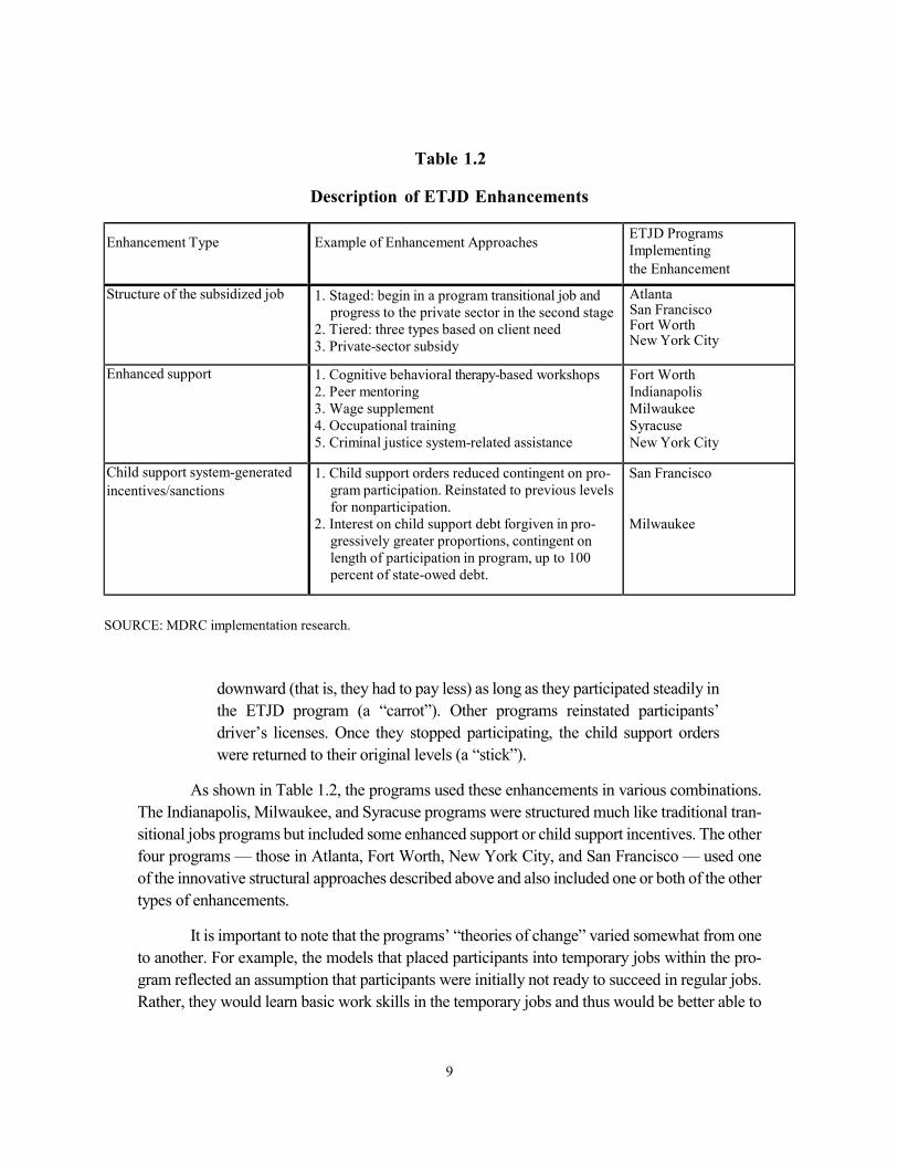
9
Table 1.2
Description of ETJD Enhancements
Enhancement Type Example of Enhancement Approaches ETJD Programs
Implementing the Enhancement
Structure of the subsidized job 1. Staged: begin in a program transitional job and progress to the private sector in the second stage
2. Tiered: three types based on client need 3. Private-sector subsidy
Atlanta San Francisco Fort Worth New York City
Enhanced support 1. Cognitive behavioral therapy-based workshops 2. Peer mentoring 3. Wage supplement 4. Occupational training 5. Criminal justice system-related assistance
Fort Worth Indianapolis Milwaukee Syracuse New York City
Child support system-generated incentives/sanctions
1. Child support orders reduced contingent on pro-gram participation. Reinstated to previous levels for nonparticipation.
2. Interest on child support debt forgiven in pro-gressively greater proportions, contingent on length of participation in program, up to 100 percent of state-owed debt.
San Francisco Milwaukee
SOURCE: MDRC implementation research.
downward (that is, they had to pay less) as long as they participated steadily in the ETJD program (a “carrot”). Other programs reinstated participants’ driver’s licenses. Once they stopped participating, the child support orders were returned to their original levels (a “stick”).
As shown in Table 1.2, the programs used these enhancements in various combinations. The Indianapolis, Milwaukee, and Syracuse programs were structured much like traditional tran-sitional jobs programs but included some enhanced support or child support incentives. The other four programs — those in Atlanta, Fort Worth, New York City, and San Francisco — used one of the innovative structural approaches described above and also included one or both of the other types of enhancements.
It is important to note that the programs’ “theories of change” varied somewhat from one to another. For example, the models that placed participants into temporary jobs within the pro-gram reflected an assumption that participants were initially not ready to succeed in regular jobs. Rather, they would learn basic work skills in the temporary jobs and thus would be better able to
10
get and keep regular jobs. In contrast, the programs that placed participants into subsidized pri-vate-sector jobs assumed that participants were ready to work in regular jobs, but needed help getting a foot in the door. These programs sought to change employers’ hiring decisions and pro-mote a more effective transition from subsidized to unsubsidized employment. Figure 1.1 pre-sents a generic logic model describing the theory of change.
Characteristics of the Study Participants Table 1.3 presents background characteristics of the research sample. In all of the programs, the typical participant was an unmarried black or Hispanic man in his 30s or 40s, with a criminal record and limited or no recent work experience. Data collected from study participants when they entered the study show that there is considerable overlap in the two main target groups: 42 percent of participants in the programs targeting people coming home from prison were noncus-todial parents, and 40 percent of those in the programs targeting noncustodial parents had been incarcerated (though often not recently).
Almost all participants in the noncustodial parent programs and more than 80 percent of those in the programs targeting formerly incarcerated people had worked for pay at some point in the past. However, as expected, only 20 percent of the participants in the programs targeting formerly incarcerated people had any recent work experience (within the last year). Even in the programs targeting noncustodial parents, fewer than one-third of participants (28 percent) had worked for more than a year in the previous three years.
Program Implementation All of the ETJD grantees had some experience operating transitional jobs programs, but ETJD required them to expand to a larger scale and add new components or services. Thus, it is not surprising that all of them experienced some operational challenges. Some programs had diffi-culty with recruitment and some struggled to place participants into unsubsidized jobs. Moreover, some of the enhancements were not put in place as designed. Nevertheless, overall, all of the grantees implemented functioning transitional jobs programs.
One central question is whether the ETJD programs were truly “enhanced” relative to earlier models. The answer is mixed. Several of the programs successfully implemented the struc-tural changes described above. Others were able to provide enhanced services or child support incentives. At the same time, some of the enhancements did not operate as planned. For example, the Milwaukee program had intended to place many participants into occupational skills training, but the organizational partnerships needed to make this training happen never fully materialized.
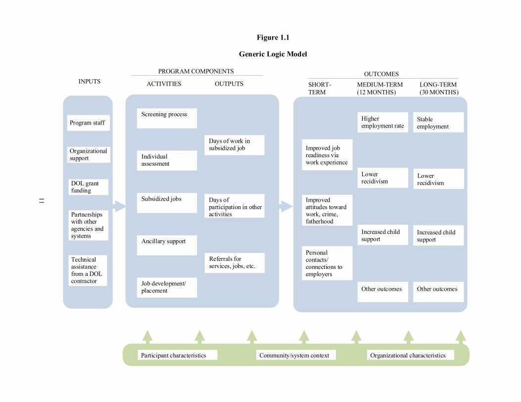
11
Figure 1.1
Generic Logic Model
Participant characteristics Community/system context Organizational characteristics
Screening process
Individual assessment
Subsidized jobs
Ancillary support
Job development/ placement
Days of work in subsidized job
Days of participation in other activities
Referrals for services, jobs, etc.
OUTPUTS
PROGRAM COMPONENTS
ACTIVITIES
Increased child support
Other outcomes
Higher employment rate
Lower recidivism
Improved attitudes toward work, crime, fatherhood
Personal contacts/connections to employers
Improved job readiness via work experience
Other outcomes
Stable employment
Lower recidivism
Increased child support
OUTCOMES MEDIUM-TERM (12 MONTHS)
SHORT-TERM
LONG-TERM (30 MONTHS)
INPUTS
Program staff
Organizational support
DOL grant funding
Partnerships with other agencies and systems
Technical assistance from a DOL contractor
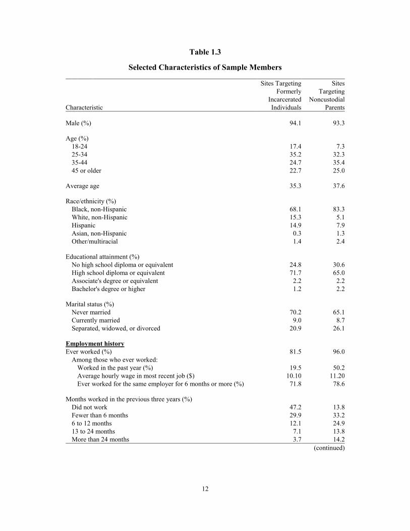
12
Table 1.3
Selected Characteristics of Sample Members
Sites Targeting Sites Formerly Targeting
Incarcerated Noncustodial Characteristic Individuals Parents
Male (%) 94.1 93.3
Age (%) 18-24 17.4 7.3 25-34 35.2 32.3 35-44 24.7 35.4 45 or older 22.7 25.0
Average age 35.3 37.6
Race/ethnicity (%) Black, non-Hispanic 68.1 83.3 White, non-Hispanic 15.3 5.1 Hispanic 14.9 7.9 Asian, non-Hispanic 0.3 1.3 Other/multiracial 1.4 2.4
Educational attainment (%) No high school diploma or equivalent 24.8 30.6 High school diploma or equivalent 71.7 65.0 Associate's degree or equivalent 2.2 2.2 Bachelor's degree or higher 1.2 2.2
Marital status (%) Never married 70.2 65.1 Currently married 9.0 8.7 Separated, widowed, or divorced 20.9 26.1
Employment history Ever worked (%) 81.5 96.0
Among those who ever worked: Worked in the past year (%) 19.5 50.2 Average hourly wage in most recent job ($) 10.10 11.20 Ever worked for the same employer for 6 months or more (%) 71.8 78.6
Months worked in the previous three years (%) Did not work 47.2 13.8 Fewer than 6 months 29.9 33.2 6 to 12 months 12.1 24.9 13 to 24 months 7.1 13.8 More than 24 months 3.7 14.2
(continued)
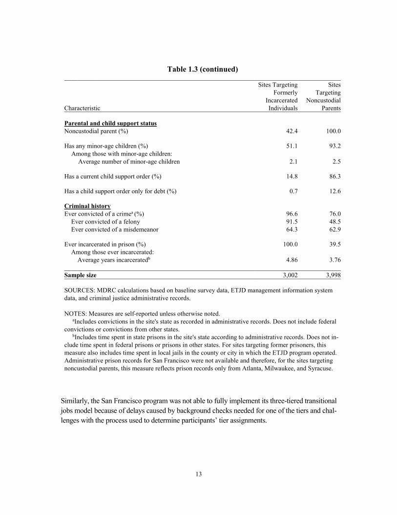
13
Table 1.3 (continued)
Sites Targeting Sites Formerly Targeting
Incarcerated Noncustodial Characteristic Individuals Parents
Parental and child support status Noncustodial parent (%) 42.4 100.0
Has any minor-age children (%) 51.1 93.2 Among those with minor-age children:
Average number of minor-age children 2.1 2.5
Has a current child support order (%) 14.8 86.3
Has a child support order only for debt (%) 0.7 12.6
Criminal history Ever convicted of a crimea (%) 96.6 76.0
Ever convicted of a felony 91.5 48.5 Ever convicted of a misdemeanor 64.3 62.9
Ever incarcerated in prison (%) 100.0 39.5 Among those ever incarcerated:
Average years incarceratedb 4.86 3.76
Sample size 3,002 3,998
SOURCES: MDRC calculations based on baseline survey data, ETJD management information system data, and criminal justice administrative records.
NOTES: Measures are self-reported unless otherwise noted. aIncludes convictions in the site's state as recorded in administrative records. Does not include federal convictions or convictions from other states. bIncludes time spent in state prisons in the site's state according to administrative records. Does not in-clude time spent in federal prisons or prisons in other states. For sites targeting former prisoners, this measure also includes time spent in local jails in the county or city in which the ETJD program operated. Administrative prison records for San Francisco were not available and therefore, for the sites targeting noncustodial parents, this measure reflects prison records only from Atlanta, Milwaukee, and Syracuse.
Similarly, the San Francisco program was not able to fully implement its three-tiered transitional jobs model because of delays caused by background checks needed for one of the tiers and chal-lenges with the process used to determine participants’ tier assignments.
14
Figure 1.2 shows the percentage of program group members who worked in a transitional job at some point during the first year after study enrollment and the average number of days that elapsed between random assignment and a participant’s first transitional-job paycheck (among those who worked in such jobs). As the figure illustrates, some programs that put participants into in-house jobs almost immediately (notably those in Indianapolis and Atlanta) provided transi-tional jobs to everyone or nearly everyone in the program group. At the other extreme, the Fort Worth program provided a range of preemployment activities and then attempted to place partic-ipants directly into subsidized private-sector jobs. In this model, the program had to persuade private employers to hire people recently released from prison (and agree to retain them after the subsidy period if all went well). Fewer than half of program group members in this model ever worked in subsidized jobs (though the program was able to place others directly into unsubsidized jobs). The programs in the middle required participants to complete some type of preemployment activity or class before starting work, or had to match participants with jobs in nonprofit agencies in the community. In either case, some participants left the programs before they were placed.
The average number of days worked in a transitional job (among those who worked) ranged from less than 30 in New York City to more than 70 in Indianapolis. To some extent, this variation reflects the programs’ designs — for example, some programs offered fewer days of work per week than others — but it also reflects the greater willingness of some programs to allow participants to stay in transitional jobs longer than planned if they had good attendance but were having difficulty finding unsubsidized jobs.
Most control group members at all sites received employment-related services; neverthe-less, there were large differences in service receipt between the program and control groups. As Figure 1.3 shows, responses to the 12-month survey indicate that, across the sites, 59 percent to 80 percent of the control group received at least some help related to finding or keeping jobs. This result is not surprising, because most of the study participants were involved with systems that expected them — and in some cases required them — to seek employment. Nevertheless, at most sites, the program group was still substantially more likely to receive employment services. In addition, based on scans of other programs available in the communities and reviews of the most common providers of control group services identified in the survey, in most cases it appears that the ETJD services were much more intensive and comprehensive than most other services avail-able.
The difference between the program and control groups in services received was smallest in Milwaukee and New York City, where about 80 percent of the control group reported receiving employment services of some kind, and the difference between the groups was less than 15 per-centage points. There were other fairly large transitional jobs programs operating in both cities at
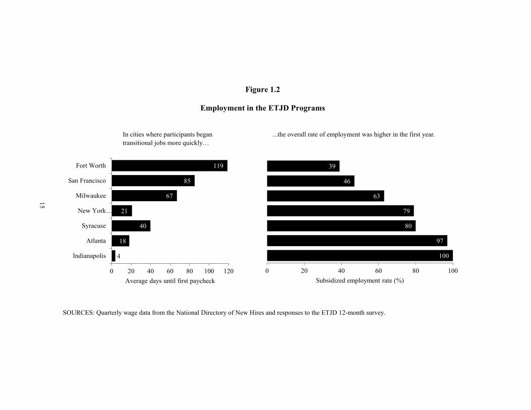
Figure 1.2
Employment in the ETJD Programs
15
In cities where participants began ...the overall rate of employment was higher in the first year.transitional jobs more quickly…
4
18
40
21
67
85
119
0 20 40 60 80 100 120
Indianapolis
Atlanta
Syracuse
New York…
Milwaukee
San Francisco
Fort Worth
Average days until first paycheck
100
97
80
79
63
46
39
0 20 40 60 80 100Subsidized employment rate (%)
SOURCES: Quarterly wage data from the National Directory of New Hires and responses to the ETJD 12-month survey.
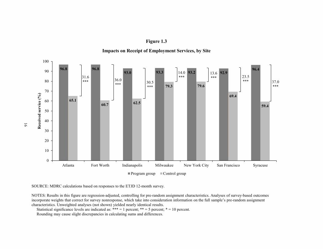
16
Figure 1.3
Impacts on Receipt of Employment Services, by Site
31.6*** 36.0
*** 30.5***
14.0***
13.6*** 23.5
*** 37.0***
96.8 96.893.0 93.3 93.2 92.9
96.4
65.160.7 62.5
79.3 79.6
69.4
59.4
0
10
20
30
40
50
60
70
80
90
100
Atlanta Fort Worth Indianapolis Milwaukee New York City San Francisco Syracuse
Rec
eive
d se
rvic
e (%
)
Program group Control group
SOURCE: MDRC calculations based on responses to the ETJD 12-month survey.
NOTES: Results in this figure are regression-adjusted, controlling for pre-random assignment characteristics. Analyses of survey-based outcomes incorporate weights that correct for survey nonresponse, which take into consideration information on the full sample’s pre-random assignment characteristics. Unweighted analyses (not shown) yielded nearly identical results.
Statistical significance levels are indicated as: *** = 1 percent; ** = 5 percent; * = 10 percent.Rounding may cause slight discrepancies in calculating sums and differences.
17
the same time as ETJD, and the research team was able to obtain data from some of those pro-grams. In New York City, about 36 percent of the ETJD control group (and 16 percent of the program group) worked in transitional jobs through the Center for Employment Opportunities, a large transitional jobs program serving individuals returning from incarceration. In Milwaukee, just over 20 percent of both the program and control groups worked in non-ETJD transitional jobs through the Transitional Jobs Demonstration Project or the Transform Milwaukee Jobs Program. It is typically much harder for a program to produce statistically significant impacts in a random assignment study if many members of the control group receive services that are similar to those being tested, and that may be what happened here.
A few site-specific findings from the implementation study are important for understand-ing the impact results discussed in later chapters:
The Atlanta program (targeting noncustodial parents) delivered most of its core compo-nents as intended, and all program group members received some level of service through the program. Staff members were generally experienced in working with the clients, appeared well acquainted with their caseloads, and consulted frequently with one another and with employment partners. Almost all program group members (97 percent) were placed into the first stage of sub-sidized employment at Goodwill Industries (the grantee, a nonprofit organization), and almost two-thirds (63 percent) worked in a second-stage subsidized job in the community. Those who worked in subsidized jobs participated for around the time periods initially intended (one month at Goodwill and three months in a second-stage external employer job). However, the program deviated from the intended model in the types and diversity of second-stage jobs that were avail-able to participants. While these positions offered exposure to real-world work environments, there were a limited number of employers working with the program at this stage and those of-fered little opportunity for advancement. Most jobs at this second stage of the program were pro-vided by a small number of retail stores and nonprofit organizations.
The Milwaukee program (targeting noncustodial parents) implemented some aspects of its model as intended but experienced challenges with staffing and with the implementation of certain components. The grantee, the YWCA, had difficulty recruiting enough participants and staff turnover affected some aspects of service delivery. Participation dropped off at various stages, and ultimately fewer than two-thirds of participants actually received transitional jobs. Further, there was a substantial delay before many of the transitional job placements, perhaps because the program sought to tailor placements to individual circumstances. An initial plan to provide many participants with occupational training was not implemented. The child support enhancement, which included forgiveness of interest on child support debt owed to the state, was well implemented, but it only affected a small proportion of the total debt participants owed. The child support enhancement also included the integration of a Legal Action attorney and the avail-

18
ability of an on-site child support representative. These features were well regarded by staff mem-bers and participants alike. While the earnings supplement appears to have been implemented, only a small portion of the program group (9 percent) received it. The low rate of receipt was in part because of program attrition, but also because the supplement was only available to individ-uals earning less than $10 per hour. Since the average wage was about $10 per hour, it is likely that many who did obtain jobs earned too much to receive the supplement. As noted earlier, a large proportion of the control group in Milwaukee reported receiving employment services and the difference between the program and control groups in service receipt was relatively small.
The San Francisco program (targeting noncustodial parents) was innovative but faced significant operational challenges. Fewer than half of the program group (44 percent) ever worked in a subsidized job. This low placement rate occurred, in part, because half of the participants were unable to complete the required preemployment activities, which included a drug test that many participants could not pass. In addition, the program struggled to identify subsidized posi-tions with private-sector employers, and there were delays in placing participants in the public-sector tier. Ultimately, among participants who were slated for the private-sector tier, only 24 percent were actually placed in that type of subsidized job (others were placed in nonprofit posi-tions); similarly, only 39 percent of those slated for the public-sector tier worked in that type of position. The Department of Child Support Services successfully provided substantial benefits to participants through its use of child support-related incentives, including the release of suspended driver’s licenses and modifications that reduced child support orders as long as participants were in good standing with the program.
The Syracuse program (targeting noncustodial parents) operated as intended, with a few modifications. However, for most of the grant period there were challenges with case manage-ment services and with cultivating employers, identifying job openings, and placing people in jobs. The adaptations made during implementation included instituting a four-month maximum for the transitional job early in the grant period due to capacity and cost constraints. Though the program had hoped to establish crews with private employers in an array of industries that might lead to unsubsidized employment, crews were only established at nonprofit or public organiza-tions with limited opportunities to hire participants in unsubsidized jobs. The program’s decen-tralized service-delivery structure probably required more resources for coordination than would be associated with a more centralized effort. While most partners demonstrated strong commit-ment to the program and its evaluation, and a willingness to address logistical and administrative challenges, some partnerships never fully materialized as envisioned.
The Fort Worth program (targeting formerly incarcerated people) provided participants with access to extensive services, including assistance with criminal records, mental health ser-vices, and a variety of preemployment services. The intended model was premised on helping
19
participants to become “job-ready” and then helping them find subsidized jobs in the private sec-tor that would turn into permanent employment with the same employer. The program’s wage-subsidy model did not place participants in transitional jobs; rather, participants had to search and interview for jobs. This approach resulted in long delays from the time participants enrolled to the time they began working, which caused considerable attrition from the program. Partway through program operations, program managers added financial incentives to stem program attri-tion, encourage engagement during preemployment activities, and deliver financial assistance to participants while they looked for jobs, but ultimately just 39 percent of program group members worked in subsidized jobs, a figure that is roughly similar to other programs using this model.16
The Indianapolis program (targeting formerly incarcerated people) achieved a high rate of participation in program services. All participants worked in transitional jobs and over 90 per-cent received work-related support. Participants reported high satisfaction with all program ser-vices. Among the noncustodial parents in the program group (about half of the sample), over 70 percent received child support assistance, including debt compromise and driver’s license rein-statement. Two small social enterprises were engaged to provide the full array of program ser-vices to 200 of the 500 program group members. While these enterprises implemented many components of the program, they were unable to replicate peer mentoring from formerly incar-cerated individuals and eventually all program group services were provided by RecycleForce (the ETJD grantee) directly. Although transitional jobs were designed to last four months, most participants requested and were granted extensions if they had not found unsubsidized work or were deemed unready for unsubsidized employment. Fifty percent of participants were in the program for more than four months. Staff members also said that while a full-time, unsubsidized job was the ultimate goal for participants, it may not have been a realistic expectation for them after four months in the program. Many participants transitioned to temporary jobs, some with the ETJD grantee, which gave workers the flexibility to attend to the requirements of probation and parole while continuing to develop workplace skills.
In the New York City program (targeting formerly incarcerated people), all of the essen-tial program components were put in place as planned, with some minor variations. The program relied heavily on parole officers for referrals and, while the program ultimately met its recruitment goal, staff members spent a great deal of time developing and tending to relationships with local parole offices. Almost all program group members received at least some ETJD services and 79 percent worked in transitional jobs. Overall, about half of the program group (two-thirds of those who worked in transitional jobs) ever worked in an internship, the second stage of subsidized employment. New York City has many services aimed at formerly incarcerated people, and, as
16See, for example, Glosser, Barden, and Williams (2016).
20
noted earlier, almost 80 percent of the control group reported receiving help with employment and 36 percent participated in another transitional jobs program in the city.
Findings in This Report The chapters that follow present longer-term impact findings and costs for the ETJD programs. Chapter 2 presents impact findings on employment and earnings outcomes for all seven ETJD programs. Chapter 3 presents impact findings on child support and family engagement outcomes for the four ETJD programs targeting noncustodial parents. Chapter 4 presents impact findings on criminal justice outcomes for the three ETJD programs targeting formerly incarcerated people. Chapter 5 presents information about the costs of operating the ETJD programs and the cost-effectiveness of the programs.17 Chapter 6 discusses the implications of the ETJD findings.
17A companion document (Foley, Farrell, Webster, and Walter, forthcoming) discusses the costs and bene-
fits of the Indianapolis ETJD program.

21
Chapter 2
Impacts on Earnings, Employment, and Material Well-Being
This chapter presents the Enhanced Transitional Jobs Demonstration (ETJD) programs’ impacts on employment and earnings after 30 months using earnings data from the National Directory of New Hires, supplemented by data from the 30-month survey of study participants.1 Using these data sources it is possible to describe employment and earnings in jobs that were reported to the unemployment insurance system (including, for some programs, employment subsidized by ETJD) and to describe job characteristics as reported by survey respondents. The final section of the chapter presents impacts on some measures of well-being that might, in theory, be affected by improvements in employment and earnings.
The chapter first discusses findings for a confirmatory outcome measuring longer-term unsubsidized earnings. Only findings for this outcome, estimated using the pooled sample of all seven ETJD sites, should be considered conclusive evidence of the effect of the ETJD programs on participants’ earnings and employment. All other results presented in this chapter should be considered exploratory.
Confirmatory Analysis ● On average, the ETJD programs increased participants’ longer-term
earnings. Program group members earned about $700 more than controlgroup members in the last year of the follow-up period.
Table 2.1 shows the programs’ impacts on the confirmatory outcome of longer-term un-subsidized earnings, averaged across all seven ETJD sites. During the final 12 months of the follow-up period (between 18 and 30 months after random assignment), unemployment insurance data show that program group members earned more than control group members: Program group
1The National Directory of New Hires primarily includes jobs covered by unemployment insurance. As such, it does not contain data on informal employment or self-employment (including contract “1099” employ-ment — that is, employment where workers are classified as independent contractors and receive income re-ported on the 1099 tax form).

22
Table 2.1
Confirmatory Impact Measure for the Employment and Earnings Domain: All Sites
Ninety Percent Program Control Difference Confidence
Outcome Group Group (Impact) Interval
Total earnings during the last year of the follow-up perioda ($) 8,298 7,597 701 *** [262, 1,140]
Sample size 3,518 3,479
SOURCE: MDRC calculations based on quarterly wage data from the National Directory of New Hires. NOTES: Results in this table are regression-adjusted, controlling for pre-random assignment characteris-tics. Statistical significance levels are indicated as: *** = 1 percent; ** = 5 percent; * = 10 percent. Rounding may cause slight discrepancies in calculating sums and differences. aThis measure of earnings during the final year of follow-up in the pooled group of all seven ETJD sites was prespecified as the confirmatory measure for the employment and earnings domain.
members earned $8,298 and control group members earned $7,597.2 The difference of $701 (an increase of about 9 percent over the control group average) is statistically significant, confirming that on average the ETJD programs increased longer-term earnings. This earnings impact is larger than the average long-term earnings impacts from several other recent studies of employment and training programs for hard-to-employ job-seekers.3
2All individuals in the ETJD sample supplied their Social Security numbers when they entered the study.
These Social Security numbers were matched against the National Directory of New Hires. If no wage records were found in the National Directory of New Hires for a Social Security number for a quarter, then employment and earnings for the individual were assumed to be zero for that quarter. An exception was made for three indi-viduals in the ETJD sample who had Social Security numbers that did not conform to Social Security Admin-istration issuance guidelines: these individuals were treated as missing for all analyses involving National Direc-tory of New Hires records.
3In a recent literature review conducted for the U.S. Health and Human Services Office of Planning, Re-search, and Evaluation, only 3 of 23 studies published between 2010 and 2014 about employment and training programs targeting hard-to-employ job seekers demonstrated positive impacts on long-term earnings (defined as earnings more than 18 months after study entry). Studies of programs involving primarily conditional cash trans-fer, parenting, or health interventions were not included in this tally, nor were programs targeting already-em-ployed individuals. See the Employment Strategies for Low-Income Adults Evidence Review, available at https://employmentstrategies.acf.hhs.gov.
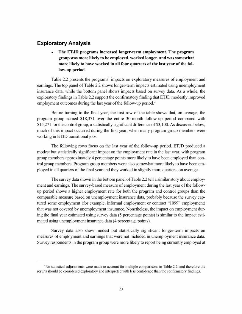
23
Exploratory Analysis ● The ETJD programs increased longer-term employment. The program
group was more likely to be employed, worked longer, and was somewhat more likely to have worked in all four quarters of the last year of the fol-low-up period.
Table 2.2 presents the programs’ impacts on exploratory measures of employment and earnings. The top panel of Table 2.2 shows longer-term impacts estimated using unemployment insurance data, while the bottom panel shows impacts based on survey data. As a whole, the exploratory findings in Table 2.2 support the confirmatory finding that ETJD modestly improved employment outcomes during the last year of the follow-up period.4
Before turning to the final year, the first row of the table shows that, on average, the program group earned $18,371 over the entire 30-month follow-up period compared with $15,271 for the control group, a statistically significant difference of $3,100. As discussed below, much of this impact occurred during the first year, when many program group members were working in ETJD transitional jobs.
The following rows focus on the last year of the follow-up period. ETJD produced a modest but statistically significant impact on the employment rate in the last year, with program group members approximately 4 percentage points more likely to have been employed than con-trol group members. Program group members were also somewhat more likely to have been em-ployed in all quarters of the final year and they worked in slightly more quarters, on average.
The survey data shown in the bottom panel of Table 2.2 tell a similar story about employ-ment and earnings. The survey-based measure of employment during the last year of the follow-up period shows a higher employment rate for both the program and control groups than the comparable measure based on unemployment insurance data, probably because the survey cap-tured some employment (for example, informal employment or contract “1099” employment) that was not covered by unemployment insurance. Nonetheless, the impact on employment dur-ing the final year estimated using survey data (5 percentage points) is similar to the impact esti-mated using unemployment insurance data (4 percentage points).
Survey data also show modest but statistically significant longer-term impacts on measures of employment and earnings that were not included in unemployment insurance data. Survey respondents in the program group were more likely to report being currently employed at
4No statistical adjustments were made to account for multiple comparisons in Table 2.2, and therefore the
results should be considered exploratory and interpreted with less confidence than the confirmatory findings.
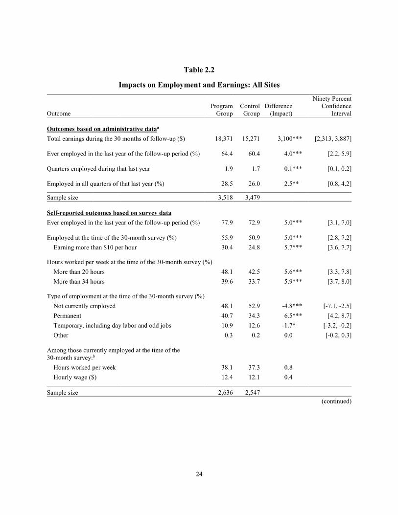
24
Table 2.2
Impacts on Employment and Earnings: All Sites
(continued)
Ninety Percent
Program Control Difference Confidence Outcome Group Group (Impact) Interval
Outcomes based on administrative dataa Total earnings during the 30 months of follow-up ($) 18,371 15,271 3,100 *** [2,313, 3,887]
Ever employed in the last year of the follow-up period (%) 64.4 60.4 4.0 *** [2.2, 5.9]
Quarters employed during that last year 1.9 1.7 0.1 *** [0.1, 0.2]
Employed in all quarters of that last year (%) 28.5 26.0 2.5 ** [0.8, 4.2]
Sample size 3,518 3,479
Self-reported outcomes based on survey data Ever employed in the last year of the follow-up period (%) 77.9 72.9 5.0 *** [3.1, 7.0]
Employed at the time of the 30-month survey (%) 55.9 50.9 5.0 *** [2.8, 7.2] Earning more than $10 per hour 30.4 24.8 5.7 *** [3.6, 7.7]
Hours worked per week at the time of the 30-month survey (%) More than 20 hours 48.1 42.5 5.6 *** [3.3, 7.8] More than 34 hours 39.6 33.7 5.9 *** [3.7, 8.0]
Type of employment at the time of the 30-month survey (%) Not currently employed 48.1 52.9 -4.8 *** [-7.1, -2.5] Permanent 40.7 34.3 6.5 *** [4.2, 8.7] Temporary, including day labor and odd jobs 10.9 12.6 -1.7 * [-3.2, -0.2] Other 0.3 0.2 0.0 [-0.2, 0.3]
Among those currently employed at the time of the 30-month survey:b
Hours worked per week 38.1 37.3 0.8 Hourly wage ($) 12.4 12.1 0.4
Sample size 2,636 2,547

25
Table 2.2 (continued) SOURCES: MDRC calculations based on quarterly wage data from the National Directory of New Hires and responses to the ETJD 30-month survey. NOTES: Results in this table are regression-adjusted, controlling for pre-random assignment characteris-tics. Analyses of survey-based outcomes incorporate weights that correct for survey nonresponse, which take into consideration information on the full sample's pre-random assignment characteristics. Un-weighted analyses (not shown) yielded nearly identical results. Statistical significance levels are indicated as: *** = 1 percent; ** = 5 percent; * = 10 percent. Rounding may cause slight discrepancies in calculating sums and differences. aEmployment rates and earnings include only jobs covered by unemployment insurance and reported to the National Directory of New Hires. bThese measures are calculated among those employed at the time of the survey; they are therefore considered nonexperimental and are not tested for statistical significance.
the time of the survey than respondents in the control group (56 percent in the program group and 51 percent in the control group), and were more likely to report having earned more than $10 per hour (30 percent versus 25 percent). Survey respondents in the program group were also more likely to have worked more than 20 hours per week and more likely to have worked more than 34 hours per week than their control group counterparts. Finally, they were more likely to report having permanent (as opposed to temporary) employment.
● ETJD substantially increased employment and earnings early in the follow-up period, when many program group members were working in transitional jobs. As expected, the magnitude of the impacts faded over time as program group members left subsidized employment, but the impacts remained statistically significant throughout the follow-up period.
Figure 2.1 shows employment and earnings over time for the program and control groups. Each of the seven programs offered temporary subsidized employment to participants early in the follow-up period, with the ultimate goal of moving participants to regular unsubsidized jobs in the longer term. The top panel of Figure 2.1 shows the ETJD programs’ impacts on overall em-ployment, which includes both ETJD subsidized employment and unsubsidized employment covered by unemployment insurance. The solid lines in the figure show the proportion of each research group that worked at least one day in each quarter of the follow-up period, starting with the quarter of random assignment, in any type of employment, including ETJD subsidized jobs. The dashed line in the figure shows the proportion of the program group that worked at least one day in an ETJD-subsidized job. The ETJD programs substantially increased employment early in
26
(continued)
Figure 2.1
Employment and Earnings Over Time: All Sites
Employment
Earnings
0102030405060708090
100
0***
1***
2***
3***
4***
5***
6***
7***
8***
9*
Perc
enta
ge e
mpl
oyed
Quarter after random assignment
Program group total employment
Control group employment
800
1,72
7
1,88
9
1,84
2
1,90
6
1,90
8
1,97
1
2,03
7
2,13
0
2,16
0
451
1,00
0 1,34
1
1,51
8
1,62
7
1,73
7
1,80
9
1,86
8
1,94
0
1,98
1
0
500
1,000
1,500
2,000
2,500
3,000
0***
1***
2***
3***
4***
5**
6**
7**
8**
9**
Ave
rage
ear
ning
s ($)
Quarter after random assignmentProgram group Control group
Program group ETJD subsidized employment
27
●
Figure 2.1 (continued)
SOURCES: MDRC calculations based on quarterly wage data from the National Directory of New Hiresand program payroll records.
NOTES: Results in this figure are regression-adjusted, controlling for pre-random assignment characteristics.
Statistical significance levels are indicated as: *** = 1 percent; ** = 5 percent; * = 10 percent.Employment rates and earnings in the quarter of random assignment through Quarter 5 after random
assignment include both ETJD subsidized jobs and jobs covered by unemployment insurance and reported to the National Directory of New Hires. Employment rates and earnings in Quarters 6 through 9 after random assignment include only jobs covered by unemployment insurance and reported to the National Directory of New Hires.
the follow-up period. The impacts faded as program group members left subsidized employment but remained statistically significant in every quarter. The convergence of the program and con-trol group employment rates appears to reflect two factors: program group members leaving sub-sidized employment, and additional control group members gradually finding employment over time. Nevertheless, by the end of the follow-up period, the employment rate was under 50 percent in each group.
The bottom panel of Figure 2.1 shows earnings over time, including both ETJD subsi-dized earnings and unsubsidized earnings in jobs covered by unemployment insurance. The pat-tern there is similar: there was a significant difference between the earnings of the program group and the control group in every quarter. However, the magnitude of that difference gradually de-clined from $727 in the first full quarter after random assignment to $179 in the last quarter of the follow-up period.
When considered individually, two ETJD programs, those in Indianapo-lis and San Francisco, produced statistically significant positive impacts on both employment and earnings in the last year of the follow-up period. Two other programs, those in Atlanta and Syracuse, had impacts on one measure but not the other. The other three programs (those in Fort Worth, New York City, and Milwaukee) did not have significant impacts on employment or earnings in the final year.
Figure 2.2 shows employment rates in the last year of the follow-up period for each of the seven ETJD programs, separately for the program and control groups, along with the esti-mated site-specific impacts. Although many of the differences in impacts among sites are not statistically significant, some patterns may be useful to explore. In Atlanta, Indianapolis, and San Francisco, the program group was more likely than the control group to work during the final
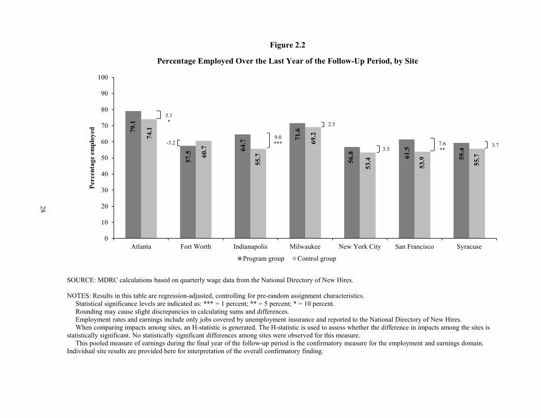
28
Figure 2.2
Percentage Employed Over the Last Year of the Follow-Up Period, by Site
SOURCE: MDRC calculations based on quarterly wage data from the National Directory of New Hires.
NOTES: Results in this table are regression-adjusted, controlling for pre-random assignment characteristics.Statistical significance levels are indicated as: *** = 1 percent; ** = 5 percent; * = 10 percent.Rounding may cause slight discrepancies in calculating sums and differences.Employment rates and earnings include only jobs covered by unemployment insurance and reported to the National Directory of New Hires.When comparing impacts among sites, an H-statistic is generated. The H-statistic is used to assess whether the difference in impacts among the sites is
statistically significant. No statistically significant differences among sites were observed for this measure.This pooled measure of earnings during the final year of the follow-up period is the confirmatory measure for the employment and earnings domain.
Individual site results are provided here for interpretation of the overall confirmatory finding.
5.1 *
-3.29.0***
3.5
2.5
7.6**
3.7
79.1
57.5 64
.7 71.6
56.8 61
.5
59.4
74.1
60.7
55.7
69.2
53.4
53.9 55.7
0
10
20
30
40
50
60
70
80
90
100
Atlanta Fort Worth Indianapolis Milwaukee New York City San Francisco Syracuse
Perc
enta
ge e
mpl
oyed
Program group Control group
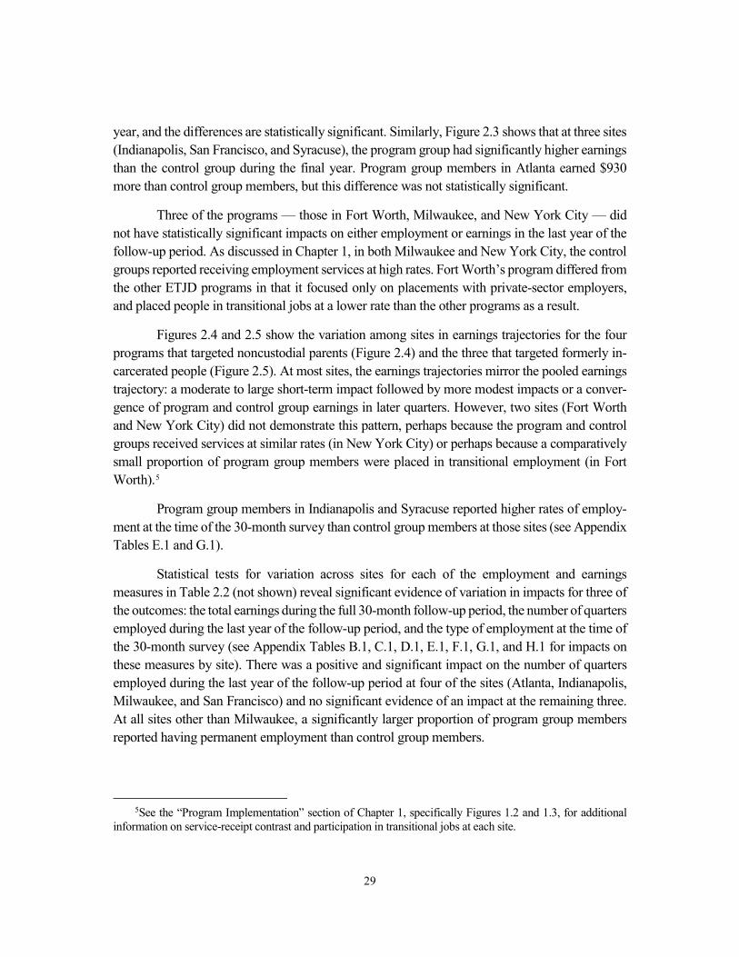
29
year, and the differences are statistically significant. Similarly, Figure 2.3 shows that at three sites (Indianapolis, San Francisco, and Syracuse), the program group had significantly higher earnings than the control group during the final year. Program group members in Atlanta earned $930 more than control group members, but this difference was not statistically significant.
Three of the programs — those in Fort Worth, Milwaukee, and New York City — did not have statistically significant impacts on either employment or earnings in the last year of the follow-up period. As discussed in Chapter 1, in both Milwaukee and New York City, the control groups reported receiving employment services at high rates. Fort Worth’s program differed from the other ETJD programs in that it focused only on placements with private-sector employers, and placed people in transitional jobs at a lower rate than the other programs as a result.
Figures 2.4 and 2.5 show the variation among sites in earnings trajectories for the four programs that targeted noncustodial parents (Figure 2.4) and the three that targeted formerly in-carcerated people (Figure 2.5). At most sites, the earnings trajectories mirror the pooled earnings trajectory: a moderate to large short-term impact followed by more modest impacts or a conver-gence of program and control group earnings in later quarters. However, two sites (Fort Worth and New York City) did not demonstrate this pattern, perhaps because the program and control groups received services at similar rates (in New York City) or perhaps because a comparatively small proportion of program group members were placed in transitional employment (in Fort Worth).5
Program group members in Indianapolis and Syracuse reported higher rates of employ-ment at the time of the 30-month survey than control group members at those sites (see Appendix Tables E.1 and G.1).
Statistical tests for variation across sites for each of the employment and earnings measures in Table 2.2 (not shown) reveal significant evidence of variation in impacts for three of the outcomes: the total earnings during the full 30-month follow-up period, the number of quarters employed during the last year of the follow-up period, and the type of employment at the time of the 30-month survey (see Appendix Tables B.1, C.1, D.1, E.1, F.1, G.1, and H.1 for impacts on these measures by site). There was a positive and significant impact on the number of quarters employed during the last year of the follow-up period at four of the sites (Atlanta, Indianapolis, Milwaukee, and San Francisco) and no significant evidence of an impact at the remaining three. At all sites other than Milwaukee, a significantly larger proportion of program group members reported having permanent employment than control group members.
5See the “Program Implementation” section of Chapter 1, specifically Figures 1.2 and 1.3, for additional
information on service-receipt contrast and participation in transitional jobs at each site.
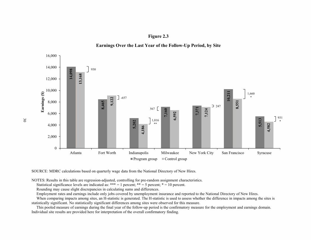
30
Figure 2.3
Earnings Over the Last Year of the Follow-Up Period, by Site
SOURCE: MDRC calculations based on quarterly wage data from the National Directory of New Hires.
NOTES: Results in this table are regression-adjusted, controlling for pre-random assignment characteristics.Statistical significance levels are indicated as: *** = 1 percent; ** = 5 percent; * = 10 percent.Rounding may cause slight discrepancies in calculating sums and differences.Employment rates and earnings include only jobs covered by unemployment insurance and reported to the National Directory of New Hires.When comparing impacts among sites, an H-statistic is generated. The H-statistic is used to assess whether the difference in impacts among the sites is
statistically significant. No statistically significant differences among sites were observed for this measure. This pooled measure of earnings during the final year of the follow-up period is the confirmatory measure for the employment and earnings domain.
Individual site results are provided here for interpretation of the overall confirmatory finding.
930
-657
567
1,016**
247
1,660*
931*
14,0
98
8,46
5
5,20
2
7,16
0
7,37
1
10,2
11
5,51
3
13,1
68
9,12
2
4,18
6
6,59
2
7,12
4 8,55
1
4,58
2
0
2,000
4,000
6,000
8,000
10,000
12,000
14,000
16,000
Atlanta Fort Worth Indianapolis Milwaukee New York City San Francisco Syracuse
Earn
ings
($)
Program group Control group
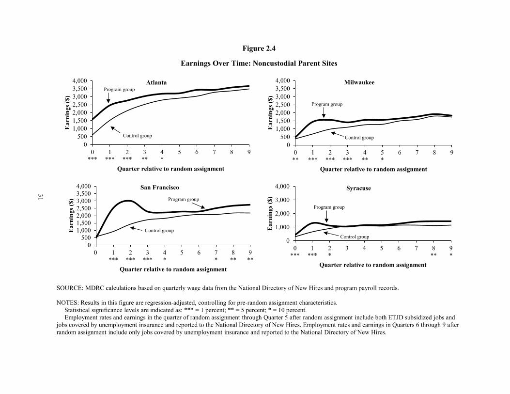
31
Earnings Over Time: Noncustodial Parent Sites
Figure 2.4
0500
1,0001,5002,0002,5003,0003,5004,000
0***
1***
2***
3**
4*
5 6 7 8 9
Earn
ings
($)
Quarter relative to random assignment
AtlantaProgram group
Control group
0500
1,0001,5002,0002,5003,0003,5004,000
0**
1***
2***
3***
4**
5*
6 7 8 9
Earn
ings
($)
Quarter relative to random assignment
Milwaukee
Program group
Control group
0500
1,0001,5002,0002,5003,0003,5004,000
0 1***
2***
3***
4*
5 6 7*
8**
9**
Earn
ings
($)
Quarter relative to random assignment
San Francisco
Program group
Control group
0
1,000
2,000
3,000
4,000
0***
1***
2*
3 4 5 6 7 8**
9*
Earn
ings
($)
Quarter relative to random assignment
Syracuse
Program group
Control group
SOURCE: MDRC calculations based on quarterly wage data from the National Directory of New Hires and program payroll records.
NOTES: Results in this figure are regression-adjusted, controlling for pre-random assignment characteristics.Statistical significance levels are indicated as: *** = 1 percent; ** = 5 percent; * = 10 percent.Employment rates and earnings in the quarter of random assignment through Quarter 5 after random assignment include both ETJD subsidized jobs and
jobs covered by unemployment insurance and reported to the National Directory of New Hires. Employment rates and earnings in Quarters 6 through 9 after random assignment include only jobs covered by unemployment insurance and reported to the National Directory of New Hires.
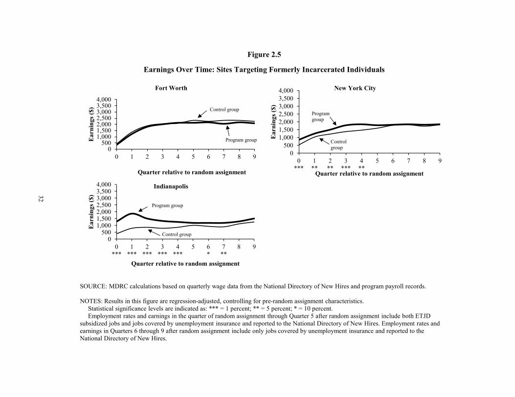
32
Earnings Over Time: Sites Targeting Formerly Incarcerated Individuals
Figure 2.5
0500
1,0001,5002,0002,5003,0003,5004,000
0 1 2 3 4 5 6 7 8 9
Earn
ings
($)
Quarter relative to random assignment
Fort Worth
Program group
Control group
0500
1,0001,5002,0002,5003,0003,5004,000
0***
1**
2**
3***
4**
5 6 7 8 9
Earn
ings
($)
Quarter relative to random assignment
New York City
Program group
Control group
0500
1,0001,5002,0002,5003,0003,5004,000
0***
1***
2***
3***
4***
5 6*
7**
8 9
Earn
ings
($)
Quarter relative to random assignment
Indianapolis
Program group
Control group
SOURCE: MDRC calculations based on quarterly wage data from the National Directory of New Hires and program payroll records.
NOTES: Results in this figure are regression-adjusted, controlling for pre-random assignment characteristics.Statistical significance levels are indicated as: *** = 1 percent; ** = 5 percent; * = 10 percent.Employment rates and earnings in the quarter of random assignment through Quarter 5 after random assignment include both ETJD
subsidized jobs and jobs covered by unemployment insurance and reported to the National Directory of New Hires. Employment rates and earnings in Quarters 6 through 9 after random assignment include only jobs covered by unemployment insurance and reported to theNational Directory of New Hires.
33
Three of the four programs that had longer-term impacts on employment outcomes had close connections with the child support agencies in their jurisdictions. The San Francisco pro-gram produced positive and significant impacts on a range of employment-related outcomes. The program experienced challenges in implementing its transitional jobs model, and did not place the majority of participants into transitional jobs. However, one aspect of the model, run by the child support enforcement agency, was well implemented: the child support agency offered spe-cific system enhancements, including reducing the amount of child support a program group par-ticipant was ordered to pay as long as he or she was in good standing and participated in the program’s services, or was employed. The reduced orders may have helped mitigate disincentives to work that are sometimes associated with lack of engagement in the formal labor market among men who owe large amounts of child support.6
The child support agency was also a partner of two of the other programs that demon-strated longer-term impacts on employment-related outcomes. The child support agencies in At-lanta and Indianapolis worked in close collaboration with the ETJD programs there, but the child support system enhancements for program group members were not as extensive in those pro-grams as they were in the San Francisco program. It is not clear why the involvement of the child support agency would have affected the impacts on employment at those two sites. The child support agency was not a major partner of the Syracuse program.
● Earnings and employment impacts do not differ substantially among im-portant subgroups of the ETJD sample. There were almost no statistically significant differences in impacts between subgroups based on recent em-ployment, noncustodial parent status, education, age, or time of study en-rollment.
The evaluation team examined whether impacts varied for subgroups of the ETJD popu-lation that were defined using baseline data collected when participants entered the study (or data from administrative records from the period before participants were randomly assigned). Ap-pendix Table A.1 shows final-year impacts separately for two subgroups of participants defined by the primary population their programs targeted: noncustodial parents or formerly incarcerated people. These two populations overlap but each faces some unique challenges, and it is possible that transitional jobs may work better for one group than for the other. In fact, impacts on earnings and employment were significantly, and substantially, larger for the programs targeting noncus-todial parents. However, additional analysis suggests that this pattern probably does not reflect the target population per se: Appendix Table A.2 shows that impacts among noncustodial parents across all programs (including those that targeted formerly incarcerated individuals) are not sig-
6Cancian, Heinrich, and Chung (2013).

34
nificantly different from those for sample members who are not noncustodial parents. The im-pacts for programs targeting formerly incarcerated people were depressed by the results from Fort Worth and New York City. As discussed earlier, neither of those programs generated statistically significant impacts on longer-term employment outcomes, but the reasons may not be related to the population they targeted.
Appendix A also shows final-year impacts separately for subgroups of participants who were and were not employed in the year before they entered the study, who did and did not have high school diplomas when they entered, who were 18 to 24 and who were 25 and older, and who joined the study in Year 1 and Year 2. All employment and earnings outcomes in Appendix Ta-bles A.1 through A.6 were measured using administrative data. Briefly:
o
o
Appendix Table A.3 shows impacts among study participants who worked in the year before they enrolled in the study and among those who did not. Recent employment can signal to employers that an individ-ual is more employable. The hypothesis behind this subgroup analysis is that participants who were less connected to the labor market might ben-efit more from transitional jobs than those who had worked recently (and who therefore already had recent experience and skills to draw upon when seeking employment). This analysis was limited to the four pro-grams targeting noncustodial parents.7 In both the program and control groups, study participants with recent work experience had better longer-term employment and earnings outcomes than those who did not. How-ever, there were no statistically significant differences in impacts be-tween the two subgroups.
Appendix Table A.4 shows impacts among participants who did not have high school diplomas when they entered the study and among partici-pants who did. As the program and control group outcomes in the table confirm, high school graduates tended to have higher earnings than non-graduates. The impacts on earnings over the full 30-month follow-up pe-riod and on employment in the final year of the follow-up period appear to be somewhat larger among nongraduates than among graduates, but the estimates of impacts on earnings in the final year for the two groups are not significantly different from one another. However, the difference
7Although 20 percent of individuals at sites targeting former prisoners had worked at some point in the year
before they entered the study, all spent the majority of the year incarcerated and out of the labor market. This subgroup analysis is therefore limited to the programs targeting noncustodial parents, the vast majority of whom were not incarcerated in the year before they entered the study and were therefore potentially able to participate in the labor market.
35
in impacts on employment during the last year of the follow-up period among the two groups was statistically significant, with greater impacts (8 percentage points) among those who did not have high school diplo-mas than among those who did have high school diplomas (3 percentage points). There were no statistically significant differences in impacts on measures of child support or criminal justice between high school gradu-ates and nongraduates.
o
o
Appendix Table A.5 shows final-year impacts among participants who were 18 to 24 years old when they enrolled in the study and participants who were 25 or older. The idea underlying this subgroup analysis is that young adults who are neither in school nor working are typically more difficult to engage in program services than older adults, are less likely than older adults to pay child support, and have higher rates of recidivism if they are involved in the criminal justice system. Therefore, younger adults may have different experiences with transitional jobs programs. They may benefit more from them because they are at higher risk. Alter-natively, older adults may benefit more because they are easier to engage in services and have reached a point in their lives when they may be more receptive to services.8 The impacts among older study participants appear to be substantially larger than those among younger participants for each of the five measures of earnings and employment shown in the table. Again, however, the difference in impacts between subgroups was not statistically significant, meaning that these differences could be due to chance. The small size of the 18-to-24-year-old subgroup (812 study participants) substantially limits the statistical precision of this analysis.
Impacts were also examined among participants who enrolled during the first year of the study and those who enrolled during the second year. The ETJD programs may have strengthened over time, which could translate into stronger impacts among those who enrolled later. Appendix Table A.6 shows that while impacts were slightly larger among those who enrolled in the second year, once again the differences between im-pact estimates are not statistically significant.
● On average, there were few impacts on measures of material hardship, health, emotional well-being, or social support at the end of the follow-up period. However, a reduction in the receipt of food stamps and an increase
8Uggen (2000).

36
in employer-sponsored health insurance may be tied to the increases in employment discussed earlier.
Given that the impacts on employment and earnings at the end of the follow-up period were generally modest in size, one might not expect to see large effects on measures of personal well-being at that point. Many of these outcomes were also measured 12 months after random assignment, closer to the time when program group members had been working in transitional jobs. At that point several of the programs produced impacts on important indicators of well-being.9 In addition, at two of the ETJD sites (Atlanta and San Francisco), an even earlier survey was administered during the time when many program group members were still working in tran-sitional jobs. Data from that survey also showed significant impacts on some measures of well-being.10
Table 2.3 shows that there were few differences between the program and control groups in measures of material hardship 30 months after random assignment. Notably, a large proportion of participants in both the program and control groups reported experiencing one or more finan-cial shortfalls (approximately 60 percent in both groups), with approximately 40 percent in each group reporting an inability to pay their rent or mortgage, and more than a third of each group reporting that their utility or phone service had been disconnected in the past year.
Table 2.3 also shows that the program group was about 5 percentage points less likely than the control group to have received Supplemental Nutrition Assistance Program benefits (also known as food stamps) in the month before the survey. It is possible that program group members were less likely to be eligible for food stamps due to their slightly higher employment and earn-ings in the last quarter of the follow-up period.
Table 2.4 shows the ETJD programs’ effects on measures of health, well-being, and so-cial support. Just under three-quarters of study participants in both research groups reported being in good health (or better), and a similar proportion in both groups reported being pretty happy or very happy at the time of the 30-month survey. Nonetheless, participants in both groups reported having experienced serious psychological stress in the past month. A greater proportion of the control group than the program group reported high psychological stress (13 percent of the pro-gram group versus 15 percent of the control group).
9Redcross et al. (2016). 10Redcross et al. (2016).
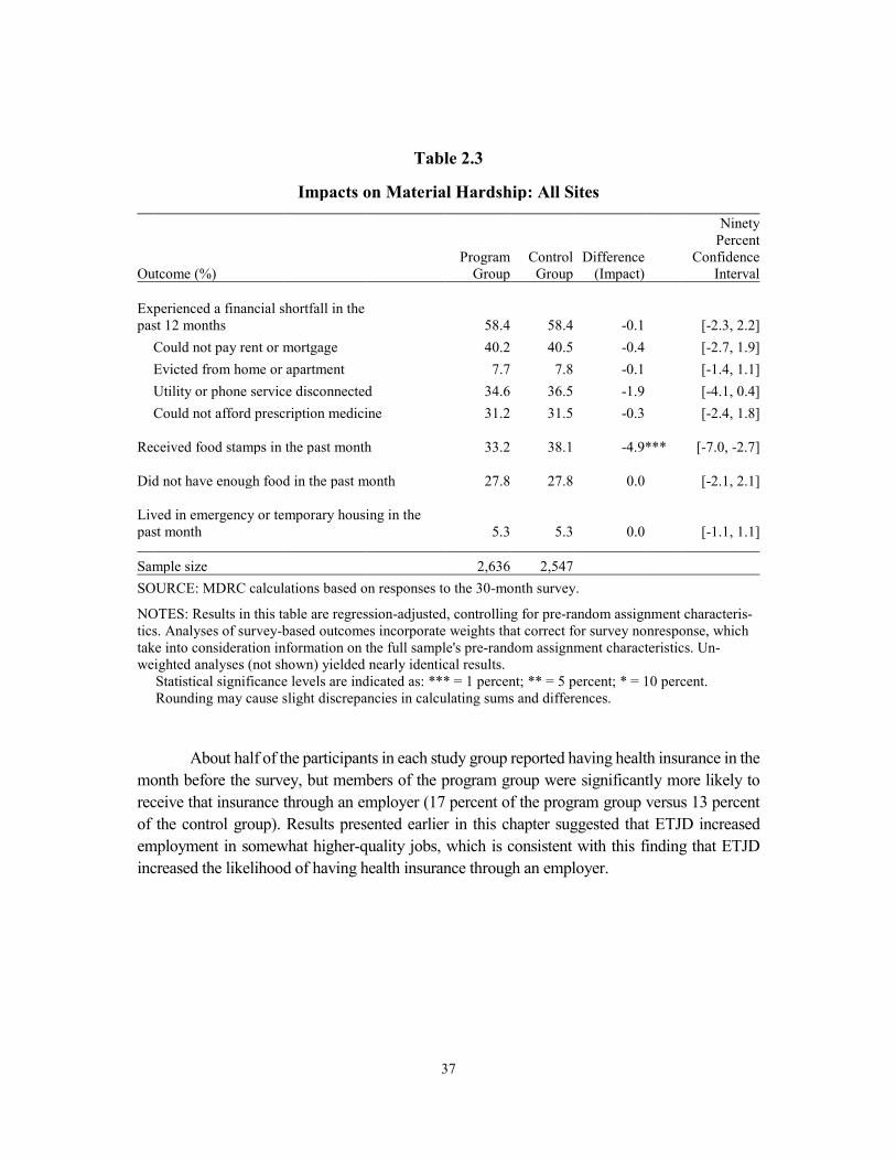
37
Table 2.3
Impacts on Material Hardship: All Sites
Ninety Percent
Program Control Difference Confidence Outcome (%) Group Group (Impact) Interval
Experienced a financial shortfall in the past 12 months 58.4 58.4 -0.1 [-2.3, 2.2]
Could not pay rent or mortgage 40.2 40.5 -0.4 [-2.7, 1.9] Evicted from home or apartment 7.7 7.8 -0.1 [-1.4, 1.1] Utility or phone service disconnected 34.6 36.5 -1.9 [-4.1, 0.4] Could not afford prescription medicine 31.2 31.5 -0.3 [-2.4, 1.8]
Received food stamps in the past month 33.2 38.1 -4.9 *** [-7.0, -2.7]
Did not have enough food in the past month 27.8 27.8 0.0 [-2.1, 2.1]
Lived in emergency or temporary housing in the past month 5.3 5.3 0.0 [-1.1, 1.1]
Sample size 2,636 2,547 SOURCE: MDRC calculations based on responses to the 30-month survey.
NOTES: Results in this table are regression-adjusted, controlling for pre-random assignment characteris-tics. Analyses of survey-based outcomes incorporate weights that correct for survey nonresponse, which take into consideration information on the full sample's pre-random assignment characteristics. Un-weighted analyses (not shown) yielded nearly identical results. Statistical significance levels are indicated as: *** = 1 percent; ** = 5 percent; * = 10 percent. Rounding may cause slight discrepancies in calculating sums and differences.
About half of the participants in each study group reported having health insurance in the month before the survey, but members of the program group were significantly more likely to receive that insurance through an employer (17 percent of the program group versus 13 percent of the control group). Results presented earlier in this chapter suggested that ETJD increased employment in somewhat higher-quality jobs, which is consistent with this finding that ETJD increased the likelihood of having health insurance through an employer.

38
Table 2.4
Impacts on Health, Well-Being, and Social Support: All Sites
e
Ninety Percent Program Control Differenc Confidence
Outcome Group Group (Impact) Interval
Is currently in good, very good, or excellent health (%) 73.9 71.9 2.0 [0.0, 3.9]
Had health insurance coverage in the past month (%) 52.8 51.3 1.5 [-0.8, 3.8] Health insurance coverage was employer-based 16.7 13.0 3.7 *** [2.1, 5.4]
Is currently happy (%) Very happy 19.8 20.0 -0.2 [-2.0, 1.7] Pretty happy 55.6 53.6 1.9 [-0.4, 4.2] Not too happy 24.6 26.4 -1.8 [-3.7, 0.2]
Experienced serious psychological distress in the past montha (%) 13.4 15.1 -1.6 * [-3.2, 0.0]
Emotional support network scoreb 3.7 3.6 0.1 [0.0, 0.1]
Sample size 2,636 2,547 SOURCE: MDRC calculations based on responses to the 30-month survey. NOTES: Results in this table are regression-adjusted, controlling for pre-random assignment characteristics. Anal-yses of survey-based outcomes incorporate weights that correct for survey nonresponse, which take into considera-tion information on the full sample's pre-random assignment characteristics. Unweighted analyses (not shown) yielded nearly identical results. Statistical significance levels are indicated as: *** = 1 percent; ** = 5 percent; * = 10 percent. Rounding may cause slight discrepancies in calculating sums and differences aPercentage of respondents indicating serious psychological distress is based on the Kessler-6 (K-6) scale. A score of 13 or higher on the K-6 scale is used here to define serious psychological distress. The K-6 assesses how often during the past month a respondent felt so sad that nothing could cheer him or her up, nervous, restless or fidgety, hopeless, that everything was an effort, or worthless. As a result of minor differences between the scale used to ad-minister the K-6 in the 12-month survey and the standard K-6 scale, the percentages presented in this table may slightly underestimate the incidence of serious psychological distress in this sample. bScores on the Emotional/Informational Social Support subscale from the RAND Medical Outcomes Study range from 1 (weak emotional support network) to 5 (strong emotional support network). The Emotional/Informational So-cial Support instrument assesses how often respondents have someone: they can count on to listen to them when they need to talk; to give them information to help them understand a situation; to give them good advice about a crisis; to confide in or talk to about themselves or their problems; whose advice they really want; to share their most private worries and fears with; to turn to for suggestions about how to deal with a personal problem; or who understands their problems. For additional documentation please see Sherbourne and Stewart (1993) and Moser et al. (2012).
39
The measures in Tables 2.3 and 2.4 were examined by site and some interesting patterns emerged. These findings are presented in Appendix Figures J.1, J.2, and J.3. Notably, the San Francisco program substantially reduced financial shortfalls and increased employer-provided health insurance, two important measures of economic well-being. As discussed earlier, that pro-gram produced increases in employment and earnings in the last year of the follow-up period and, in addition, program group members’ child support orders were modified downward as an incen-tive to participate in the program.11
See Appendix Tables B.4, C.4, D.4, E.4, F.5, G.5, and H.5 for impacts on measures of material hardship at each of the sites and Appendix Tables B.5, C.5, D.5, E.5, F.6, G.6, and H.6 for measures of health, well-being, and social support.
11As will be discussed in the next chapter, San Francisco program group members did not pay more child
support than their control group counterparts in the last year of the follow-up period, even though they had higher earnings.

THIS PAGE INTENTIONALLY LEFT BLANK
41
Chapter 3
Impacts on Child Support and Family Engagement
As discussed in Chapter 1, the Enhanced Transitional Jobs Demonstration (ETJD) programs — particularly those that targeted noncustodial parents — aimed to increase the payment of child support, an outcome that is typically tied to employment since most child support is deducted directly from workers’ paychecks. This chapter presents impacts after 30 months on child support payments in the four ETJD programs targeting noncustodial parents. As in Chapter 2, this chapter first discusses findings from a confirmatory analysis and then discusses findings from exploratory analyses, including differences in impacts among sites and subgroups. The chapter also discusses measures of engagement between noncustodial parents and their children.
Confirmatory Analysis The confirmatory measure chosen for the child support domain was the amount of formal child support paid in the final year of the follow-up period.1 This measure was selected because these payments should have occurred after the vast majority of ETJD program group participants left their subsidized jobs, meaning that any differences in child support payments between the pro-gram and control groups during this final year would probably not be due to subsidized earnings directly.
● On average, the four ETJD programs targeting noncustodial parents did not have a statistically significant impact on the amount of child support paid during the final year of the follow-up period.
Table 3.1 shows impacts on the confirmatory measure of longer-term child support pay-ments for the four ETJD programs targeting noncustodial parents. During the final 12 months of the follow-up period (between 18 and 30 months after random assignment), administrative child support data show that program and control group members paid similar amounts of child sup-port: Program group members paid $1,309 on average and control group members paid $1,266 on average. The difference between these amounts ($43) is neither substantively nor statistically significant, which means that on average the ETJD programs targeting noncustodial parents did not result in longer-term, sustained impacts on child support payment amounts.
1Formal child support was selected rather than informal because the ETJD models focused on moving par-
ticipants into the formal labor economy; exploratory measures of informal child support are presented later in the chapter.
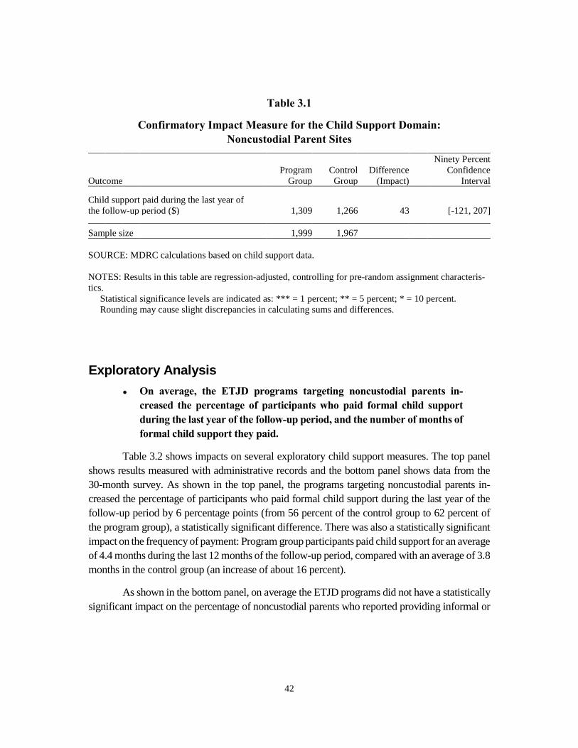
42
Table 3.1
Confirmatory Impact Measure for the Child Support Domain: Noncustodial Parent Sites
Ninety Percent
Program Control Difference Confidence Outcome Group Group (Impact) Interval
Child support paid during the last year of the follow-up period ($) 1,309 1,266 43 [-121, 207]
Sample size 1,999 1,967 SOURCE: MDRC calculations based on child support data. NOTES: Results in this table are regression-adjusted, controlling for pre-random assignment characteris-tics. Statistical significance levels are indicated as: *** = 1 percent; ** = 5 percent; * = 10 percent. Rounding may cause slight discrepancies in calculating sums and differences.
Exploratory Analysis ● On average, the ETJD programs targeting noncustodial parents in-
creased the percentage of participants who paid formal child support during the last year of the follow-up period, and the number of months of formal child support they paid.
Table 3.2 shows impacts on several exploratory child support measures. The top panel shows results measured with administrative records and the bottom panel shows data from the 30-month survey. As shown in the top panel, the programs targeting noncustodial parents in-creased the percentage of participants who paid formal child support during the last year of the follow-up period by 6 percentage points (from 56 percent of the control group to 62 percent of the program group), a statistically significant difference. There was also a statistically significant impact on the frequency of payment: Program group participants paid child support for an average of 4.4 months during the last 12 months of the follow-up period, compared with an average of 3.8 months in the control group (an increase of about 16 percent).
As shown in the bottom panel, on average the ETJD programs did not have a statistically significant impact on the percentage of noncustodial parents who reported providing informal or

43
Table 3.2
Impacts on Child Support and Family Relationships: Noncustodial Parent Sites
Ninety Percent Program Control Difference Confidence
Outcome Group Group (Impact) Interval
Outcomes based on administrative data Amount of formal child support paid in the last year of the follow-up period ($) 1,309 1,266 43 [-121, 207]
Paid any formal child support in that last yeara (%) 61.9 55.6 6.3 *** [3.9, 8.7]
Months of formal child support paid in that last year 4.4 3.8 0.6 *** [0.3, 0.8]
Among those who paid formal child support: Months from random assignment to first paymentb 4.5 6.8 -2.3
Sample size 1,999 1,967
Self-reported outcomes based on survey data (%) Currently a noncustodial parent of a minor-age child 65.9 65.3 0.6 [-2.1, 3.3]
Provided informal cash support or noncash support in the past month 48.9 49.0 -0.1 [-3.0, 2.8]
Informal cash support 38.1 35.9 2.3 [-0.6, 5.1] Noncash support 45.3 46.2 -0.9 [-3.8, 2.0]
Owing child support affects willingness to take jobs 22.4 21.1 1.4 [-1.5, 4.3]
Incarcerated for not paying child support 3.0 3.6 -0.6 [-1.7, 0.5]
Sample size 1,743 1,680
SOURCES: MDRC calculations based on child support agency data and responses to the ETJD 12-month and 30-month surveys. NOTES: Results in this table are regression-adjusted, controlling for pre-random assignment characteristics. Anal-yses of survey-based outcomes incorporate weights that correct for survey nonresponse, which take into considera-tion information on the full sample's pre-random assignment characteristics. Unweighted analyses (not shown) yielded nearly identical results. Statistical significance levels are indicated as: *** = 1 percent; ** = 5 percent; * = 10 percent. Rounding may cause slight discrepancies in calculating sums and differences. aMeasures of formal child support include all payments made through the state's child support collection and dis-bursement unit, including funds from employer withholding and other sources (for example, tax intercepts). bThis measure is calculated among those who paid child support during the follow-up period; it is therefore con-sidered nonexperimental and is not tested for statistical significance.

44
noncash support, or the percentage who reported being incarcerated for not paying child support (3 percent to 4 percent in both research groups reported being incarcerated for nonpayment). It is interesting to note that the increase in the proportion of parents paying formal support does not appear to have caused a decrease in the proportion who reported providing informal support, which can sometimes occur. Nearly half of both research groups reported providing some form of informal support during the month before the 30-month survey, with over one-third of sample members providing informal cash support and 45 percent providing noncash support.2
● During each quarter of the follow-up period, ETJD increased the percent-age of program group members who paid child support. ETJD also in-creased the average amount of child support paid during some early quarters, when many program group members were working in transi-tional jobs. However, the impact on the amount paid per quarter faded over time.
Figure 3.1 shows formal child support payment rates and average payment amounts for the program and control groups in the quarter of random assignment and each of the nine quarters of the follow-up period. This figure provides additional information and context for understand-ing the confirmatory measure discussed earlier. As the top panel of the figure shows, on average the four ETJD programs targeting noncustodial parents increased the percentage of program group members who paid any child support during every quarter of the follow-up period relative to the control group. The impact was largest in the early quarters, when program group members were most likely to be in transitional jobs, and lessened over time, though it remained statistically significant in all quarters.
The bottom panel of Figure 3.1 shows that increases in the amount of child support paid per quarter were concentrated in the early part of the follow-up period, when program group members were most likely to be working in transitional jobs, with a statistically significant impact of $149 of formal child support paid on average in Quarter 1 after random assignment and $111 in Quarter 2. The impacts on the amount of child support paid declined after that.
That the programs increased the percentage of noncustodial parents who paid child sup-port during the later quarters without a corresponding statistically significant increase in the av-erage amount of child support paid indicates that although more noncustodial parents in the pro-gram group were paying at least some child support, program group payers paid less than control group payers. One possible explanation for this pattern is that program group members in San
2Informal child support is measured based on reports from the noncustodial parent. Custodial parents were
not interviewed and thus there are no measures of informal child support from their perspectives.
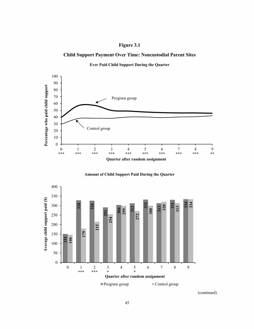
45
Figure 3.1
Child Support Payment Over Time: Noncustodial Parent Sites
(continued)
Ever Paid Child Support During the Quarter
Amount of Child Support Paid During the Quarter
0102030405060708090
100
0***
1***
2***
3***
4***
5***
6***
7***
8***
9**
Perc
enta
ge w
ho p
aid
child
supp
ort
Quarter after random assignment
Program group
Control group
151
328
326
291 30
4 312 33
2
313 33
1
334
146 17
9 215
254
299
272 30
0 320
313 33
4
0
50
100
150
200
250
300
350
400
0 1***
2***
3*
4 5*
6 7 8 9
Ave
rage
chi
ld su
ppor
t pai
d ($
)
Quarter after random assignment
Program group Control group
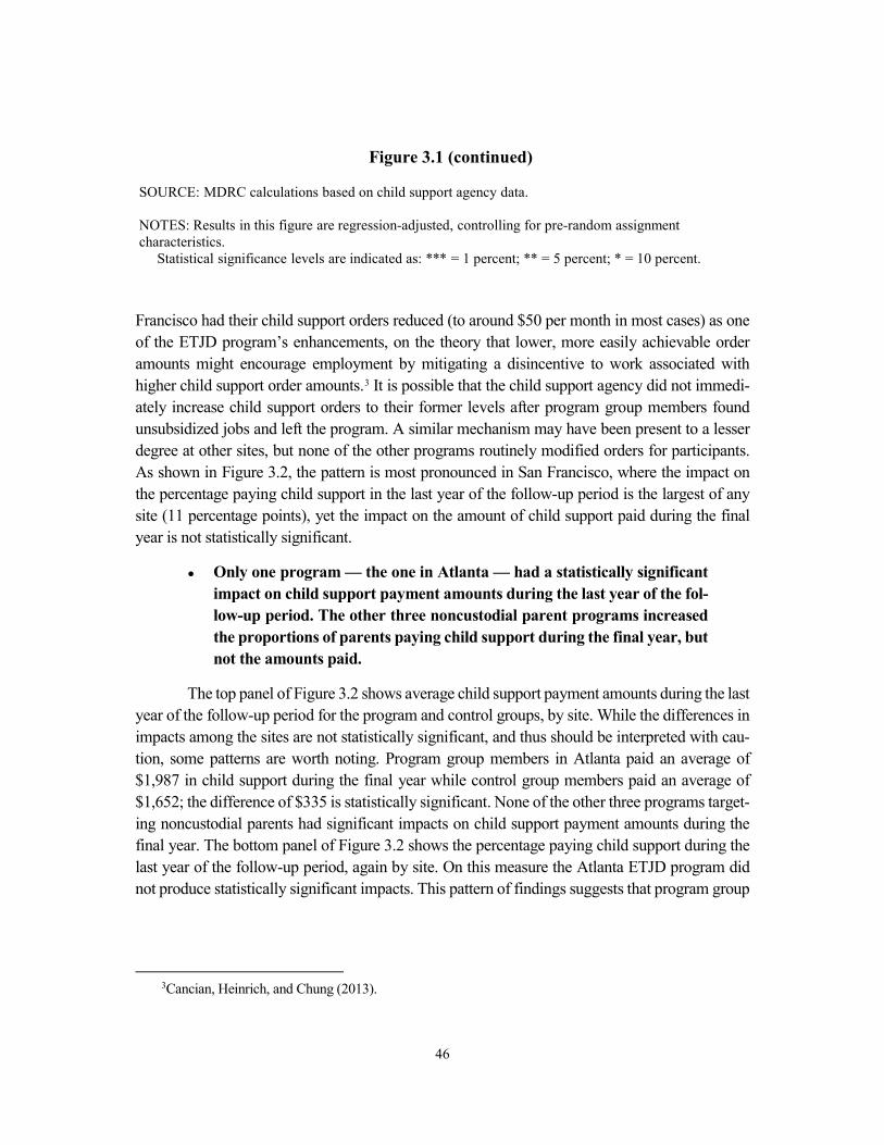
46
Figure 3.1 (continued)
SOURCE: MDRC calculations based on child support agency data.
NOTES: Results in this figure are regression-adjusted, controlling for pre-random assignment characteristics.
Statistical significance levels are indicated as: *** = 1 percent; ** = 5 percent; * = 10 percent.
Francisco had their child support orders reduced (to around $50 per month in most cases) as one of the ETJD program’s enhancements, on the theory that lower, more easily achievable order amounts might encourage employment by mitigating a disincentive to work associated with higher child support order amounts.3 It is possible that the child support agency did not immedi-ately increase child support orders to their former levels after program group members found unsubsidized jobs and left the program. A similar mechanism may have been present to a lesser degree at other sites, but none of the other programs routinely modified orders for participants. As shown in Figure 3.2, the pattern is most pronounced in San Francisco, where the impact on the percentage paying child support in the last year of the follow-up period is the largest of any site (11 percentage points), yet the impact on the amount of child support paid during the final year is not statistically significant.
● Only one program — the one in Atlanta — had a statistically significant impact on child support payment amounts during the last year of the fol-low-up period. The other three noncustodial parent programs increased the proportions of parents paying child support during the final year, but not the amounts paid.
The top panel of Figure 3.2 shows average child support payment amounts during the last year of the follow-up period for the program and control groups, by site. While the differences in impacts among the sites are not statistically significant, and thus should be interpreted with cau-tion, some patterns are worth noting. Program group members in Atlanta paid an average of $1,987 in child support during the final year while control group members paid an average of $1,652; the difference of $335 is statistically significant. None of the other three programs target-ing noncustodial parents had significant impacts on child support payment amounts during the final year. The bottom panel of Figure 3.2 shows the percentage paying child support during the last year of the follow-up period, again by site. On this measure the Atlanta ETJD program did not produce statistically significant impacts. This pattern of findings suggests that program group
3Cancian, Heinrich, and Chung (2013).
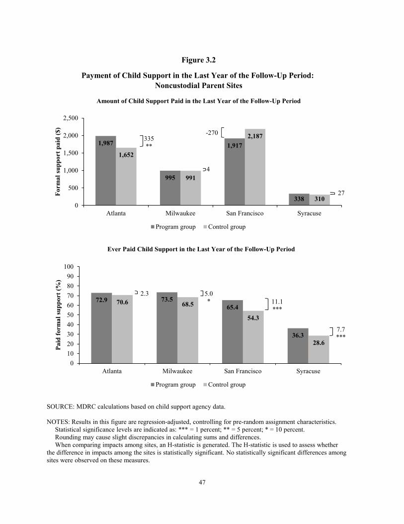
47
Figure 3.2
Payment of Child Support in the Last Year of the Follow-Up Period: Noncustodial Parent Sites
Ever Paid Child Support in the Last Year of the Follow-Up Period
Amount of Child Support Paid in the Last Year of the Follow-Up Period
2.3 5.0* 11.1
***
7.7***
72.9 73.565.4
36.3
70.6 68.5
54.3
28.6
0102030405060708090
100
Atlanta Milwaukee San Francisco Syracuse
Paid
form
al su
ppor
t (%
)
Program group Control group
335**
4
-270
27
1,987
995
1,917
338
1,652
991
2,187
3100
500
1,000
1,500
2,000
2,500
Atlanta Milwaukee San Francisco Syracuse
Form
al s
uppo
rt p
aid
($)
Program group Control group
SOURCE: MDRC calculations based on child support agency data.
NOTES: Results in this figure are regression-adjusted, controlling for pre-random assignment characteristics. Statistical significance levels are indicated as: *** = 1 percent; ** = 5 percent; * = 10 percent.Rounding may cause slight discrepancies in calculating sums and differences.When comparing impacts among sites, an H-statistic is generated. The H-statistic is used to assess whether
the difference in impacts among the sites is statistically significant. No statistically significant differences among sites were observed on these measures.

48
payers in Atlanta paid more than control group payers. The Milwaukee, San Francisco, and Sy-racuse ETJD programs all produced statistically significant impacts on the percentages paying child support but not on average payment amounts. As noted above, the impact on the payment rate is particularly large in San Francisco.
Figure 3.3 shows the average amount of child support paid by the program group and the control group in each quarter of the full follow-up period, by site. Program group members in Atlanta and Milwaukee paid more child support than their control group counterparts early in the follow-up period, when many program group members were working in subsidized jobs. In At-lanta, the impacts on child support payments persisted throughout the follow-up period, though the impacts were generally smaller in later quarters. The impact on payments largely faded by the end of the first year in Milwaukee. In Syracuse, there was almost no impact on child support payments during the follow-up period, even when program group members were working in tran-sitional jobs. Similarly, in San Francisco, there was no consistent impact on the amount of child support paid, even though there were impacts on the percentage paying child support throughout most of the follow-up period (see Appendix Figure D.3); this pattern is probably explained by the routine modification of child support orders for the program group, as discussed earlier.
● Impacts on child support payments do not differ substantially among sub-groups of the ETJD sample.
Appendix Tables A.4 through A.6 present impacts on child support payments for sub-groups of the ETJD sample defined by education, age, and time of study enrollment. As the tables show, the impacts on child support payments tend to be consistent with the earnings impacts described earlier, and do not differ substantially between subgroups of participants. For example, earnings and child support payments appeared higher for older sample members (those over 25) than their younger counterparts (18- to 24-year-olds), but the differences in impacts between these two subgroups are not statistically significant. Similarly, those with a high school diploma have slightly higher earnings and child support payments, on average, than their counterparts with no credential, but there is no statistically significant difference in impacts between the two subgroups in the last year of the follow-up period.
● The ETJD programs targeting noncustodial parents had few significant impacts on measures of family engagement.
Figures 3.4 through 3.6 show several measures of family engagement. In general, the ETJD programs did not provide extensive services designed to promote engagement between noncustodial parents and custodial parents, or between parents and children. Nevertheless,
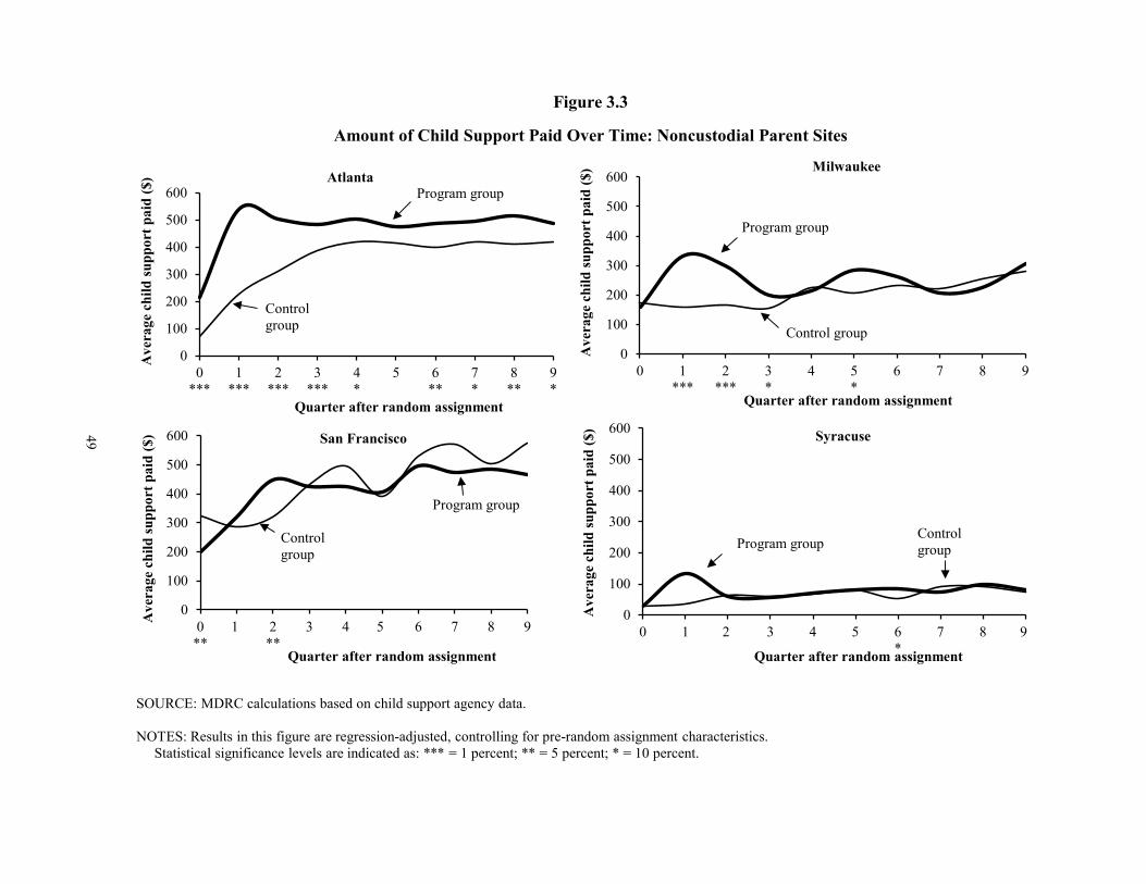
49
Figure 3.3
Amount of Child Support Paid Over Time: Noncustodial Parent Sites
0
100
200
300
400
500
600
0***
1***
2***
3***
4*
5 6**
7*
8**
9*
Ave
rage
chi
ld su
ppor
t pai
d ($
)
Quarter after random assignment
AtlantaProgram group
Control group
0
100
200
300
400
500
600
0 1***
2***
3*
4 5*
6 7 8 9
Ave
rage
chi
ld su
ppor
t pai
d ($
)
Quarter after random assignment
Milwaukee
Program group
Control group
0
100
200
300
400
500
600
0**
1 2**
3 4 5 6 7 8 9Ave
rage
chi
ld su
ppor
t pai
d ($
)
Quarter after random assignment
San Francisco
Program group
Control group
0
100
200
300
400
500
600
0 1 2 3 4 5 6*
7 8 9
Ave
rage
chi
ld su
ppor
t pai
d ($
)
Quarter after random assignment
Syracuse
Program groupControl group
SOURCE: MDRC calculations based on child support agency data.
NOTES: Results in this figure are regression-adjusted, controlling for pre-random assignment characteristics.Statistical significance levels are indicated as: *** = 1 percent; ** = 5 percent; * = 10 percent.
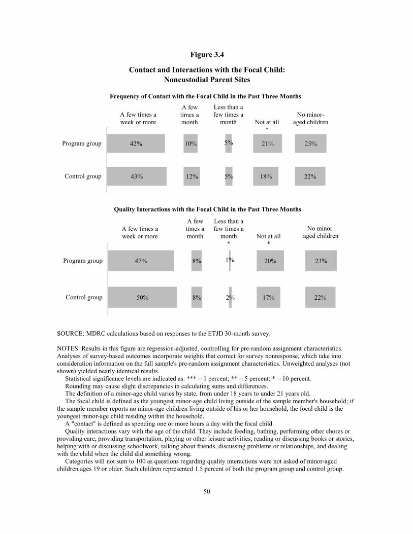
50
Figure 3.4
Contact and Interactions with the Focal Child:Noncustodial Parent Sites
43%
42%
12%
10%
5%
5%
18%
21%
22%
23%
Control group
Program group
Frequency of Contact with the Focal Child in the Past Three Months
No minor-aged children
A few times a week or more
A few times a month
Less than a few times a
month Not at all*
50%
47%
8%
8%
2%
1%
17%
20%
22%
23%
Control group
Program group
Quality Interactions with the Focal Child in the Past Three Months
No minor-aged children
A few times a week or more
A few times a month
Less than a few times a
month*
Not at all*
SOURCE: MDRC calculations based on responses to the ETJD 30-month survey.
NOTES: Results in this figure are regression-adjusted, controlling for pre-random assignment characteristics. Analyses of survey-based outcomes incorporate weights that correct for survey nonresponse, which take into consideration information on the full sample's pre-random assignment characteristics. Unweighted analyses (not shown) yielded nearly identical results.
Statistical significance levels are indicated as: *** = 1 percent; ** = 5 percent; * = 10 percent.Rounding may cause slight discrepancies in calculating sums and differences.The definition of a minor-age child varies by state, from under 18 years to under 21 years old.The focal child is defined as the youngest minor-age child living outside of the sample member's household; if
the sample member reports no minor-age children living outside of his or her household, the focal child is the youngest minor-age child residing within the household.
A "contact" is defined as spending one or more hours a day with the focal child.Quality interactions vary with the age of the child. They include feeding, bathing, performing other chores or
providing care, providing transportation, playing or other leisure activities, reading or discussing books or stories, helping with or discussing schoolwork, talking about friends, discussing problems or relationships, and dealing with the child when the child did something wrong.
Categories will not sum to 100 as questions regarding quality interactions were not asked of minor-aged children ages 19 or older. Such children represented 1.5 percent of both the program group and control group.
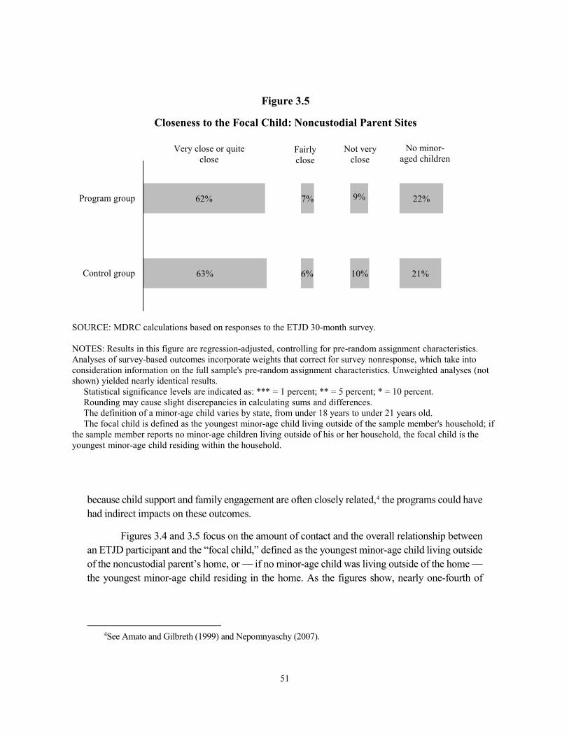
51
Figure 3.5
Closeness to the Focal Child: Noncustodial Parent Sites
63%
62%
6%
7%
10%
9%
21%
22%
Control group
Program group
No minor-aged children
Very close or quite close
Fairlyclose
Not very close
SOURCE: MDRC calculations based on responses to the ETJD 30-month survey.
NOTES: Results in this figure are regression-adjusted, controlling for pre-random assignment characteristics. Analyses of survey-based outcomes incorporate weights that correct for survey nonresponse, which take into consideration information on the full sample's pre-random assignment characteristics. Unweighted analyses (not shown) yielded nearly identical results.
Statistical significance levels are indicated as: *** = 1 percent; ** = 5 percent; * = 10 percent.Rounding may cause slight discrepancies in calculating sums and differences.The definition of a minor-age child varies by state, from under 18 years to under 21 years old.The focal child is defined as the youngest minor-age child living outside of the sample member's household; if
the sample member reports no minor-age children living outside of his or her household, the focal child is the youngest minor-age child residing within the household.
because child support and family engagement are often closely related,4 the programs could have had indirect impacts on these outcomes.
Figures 3.4 and 3.5 focus on the amount of contact and the overall relationship between an ETJD participant and the “focal child,” defined as the youngest minor-age child living outside of the noncustodial parent’s home, or — if no minor-age child was living outside of the home — the youngest minor-age child residing in the home. As the figures show, nearly one-fourth of
4See Amato and Gilbreth (1999) and Nepomnyaschy (2007).

52
Figure 3.6
Involvement in Parenting Decisions for the Focal Child:Noncustodial Parent Sites
30%
33%
21%
18%
13%
15%
14%
13%
21%
22%
Control group
Program group
Frequency of Discussing the Focal Child with the Custodial Caregiver in the Past Month
No minor-aged childrenOften
**Sometimes
***Never
Lives with the focal child
23%
24%
20%
20%
21%
21%
14%
13%
21%
22%
Control group
Program group
Current Involvement in Major Decisions About the Focal Child
No minor-aged childrenA great deal Some None
Lives with the focal child
SOURCE: MDRC calculations based on responses to the ETJD 30-month survey.
NOTES: Results in this figure are regression-adjusted, controlling for pre-random assignment characteristics. Analyses of survey-based outcomes incorporate weights that correct for survey nonresponse, which take into consideration information on the full sample's pre-random assignment characteristics. Unweighted analyses (not shown) yielded nearly identical results.
Statistical significance levels are indicated as: *** = 1 percent; ** = 5 percent; * = 10 percent.Rounding may cause slight discrepancies in calculating sums and differences.The definition of a minor-age child varies by state, from under 18 years to under 21 years old.The focal child is defined as the youngest minor-age child living outside of the sample member's household; if
the sample member reports no minor-age children living outside of his or her household, the focal child is the youngest minor-age child residing within the household.
Major decisions include decisions about such things as the focal child's education, religion, and health care.If the respondent lives with the focal child, then the respondent was not asked about involvement in parenting
decisions for the child. "Lives with the focal child" is presented as a category.
53
sample members had no minor-age children (because, for example, their youngest children may not have been minors any longer at the time of the survey).5
As shown in the top panel of Figure 3.4, most of the noncustodial parents who had minor-age children reported having fairly frequent contact with those children. For example, about two-thirds of the parents reported having contact a few times a month or more in the previous three months.6 Program group parents were slightly more likely to report not seeing their children at all; it is not clear why the ETJD programs would produce such an effect.
The bottom panel of Figure 3.4 focuses on “quality interaction” between the noncustodial parent and the focal child. “Quality interaction” is defined differently based on the age of the child but could include, for example, feeding, bathing, playing, helping with schoolwork, or discussing problems with the child. Again, most parents reported frequent quality interactions and the pro-gram group was slightly more likely to report no quality interactions. It is somewhat surprising that the percentage of parents who reported frequent quality interactions is larger than the per-centage who reported frequent contact (see the top panel of Figure 3.4). This difference may relate to the definition of “contact” used in that measure: spending one or more hours a day with the focal child. It is possible, for example, that a parent could discuss a problem with a child in a phone call that lasted less than one hour.
Figure 3.5 reports the results of a question that asked the noncustodial parent to charac-terize the closeness of his or her relationship with the focal child. Most parents reported that they were “very close or quite close” to their children, and there were no significant differences be-tween the program group and the control group.
Figure 3.6 focuses on the interactions between noncustodial parents and custodial par-ents. The top panel shows how often the noncustodial parent and the custodial parent discussed the focal child. Program group parents were slightly more likely than control group parents to report that they had such discussions “often.” This effect could be related to the increase in the number of noncustodial parents who paid child support (discussed above). The bottom panel of Figure 3.6 shows the extent to which noncustodial parents were involved in major decisions about the focal child (defined as decisions about things like education, health care, and religion). Most of the noncustodial parents who had minor-age children living outside their home reported either some or a great deal of involvement, and there were no statistically significant differences be-tween the program group and the control group.
5About one in seven ETJD sample members lived with the focal child. Those parents are included in the
results shown in Figures 3.4 and 3.5. 6This figure is calculated by adding together the percentages of parents who saw their children a few times
a week and a few times a month, and dividing by the overall percentage who had any minor-age children.

THIS PAGE INTENTIONALLY LEFT BLANK
55
Chapter 4
Impacts on Recidivism
As discussed in Chapter 1, the programs in the Enhanced Transitional Jobs Demonstration (ETJD) — particularly those that targeted people returning to the community from prison — sought to decrease recidivism. The causal link between employment and recidivism is complex, but employment services often play a central role in programs designed to improve outcomes for people reentering their communities.1 This chapter presents the impacts, after 30 months, of the three ETJD programs targeting formerly incarcerated people on measures of recidivism including arrest, conviction, and incarceration in jail and prison. As in Chapters 2 and 3, the chapter first discusses findings from a confirmatory analysis and then discusses findings from exploratory analyses. Finally, the chapter discusses differences across sites in these measures, and differences in impacts between subgroups at higher and lower risk of recidivism.
Confirmatory Analysis The confirmatory measure chosen for the criminal justice domain was whether participants had any criminal justice event during the 30-month follow-up period, with an “event” being defined as any arrest, conviction, or return to incarceration in either jail or prison. Table 4.1 shows this confirmatory measure for the three ETJD programs targeting formerly incarcerated people.
● On average, the three ETJD programs targeting formerly incarcerated individuals did not have a statistically significant impact on whether par-ticipants had a criminal justice event in the 30 months after they entered the program.
Roughly 60 percent of program and control group members across the three ETJD sites had a criminal justice event during the 30-month follow-up period. This rate of recidivism for recently released former prisoners is consistent with national averages.2
Exploratory Analysis ● On average, the three ETJD programs targeting formerly incarcerated
individuals modestly reduced felony convictions and incarceration in
1Duran, Plotkin, Potter, and Rosen (2013). 2Durose, Cooper, and Snyder (2014).
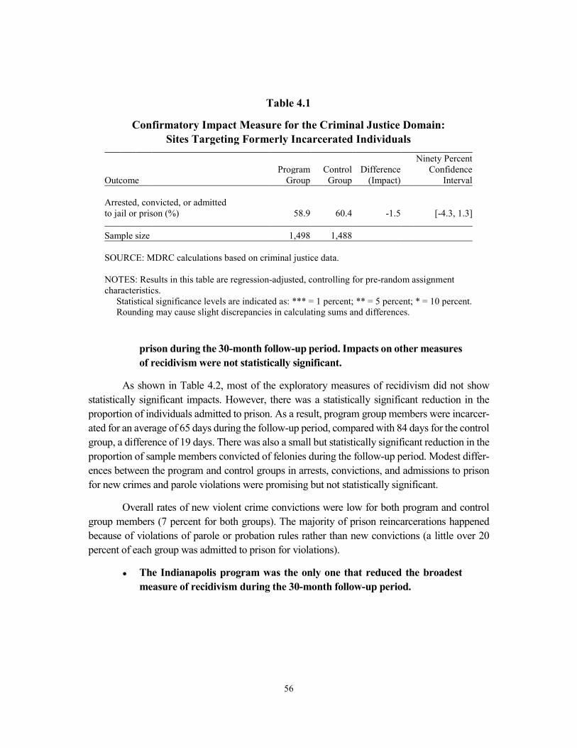
56
●
Table 4.1
Confirmatory Impact Measure for the Criminal Justice Domain: Sites Targeting Formerly Incarcerated Individuals
Ninety Percent
Program Control Difference Confidence Outcome Group Group (Impact) Interval
Arrested, convicted, or admitted to jail or prison (%) 58.9 60.4 -1.5 [-4.3, 1.3]
Sample size 1,498 1,488
SOURCE: MDRC calculations based on criminal justice data. NOTES: Results in this table are regression-adjusted, controlling for pre-random assignment characteristics. Statistical significance levels are indicated as: *** = 1 percent; ** = 5 percent; * = 10 percent. Rounding may cause slight discrepancies in calculating sums and differences.
The Indianapolis program was the only one that reduced the broadest measure of recidivism during the 30-month follow-up period.
prison during the 30-month follow-up period. Impacts on other measures of recidivism were not statistically significant.
As shown in Table 4.2, most of the exploratory measures of recidivism did not show statistically significant impacts. However, there was a statistically significant reduction in the proportion of individuals admitted to prison. As a result, program group members were incarcer-ated for an average of 65 days during the follow-up period, compared with 84 days for the control group, a difference of 19 days. There was also a small but statistically significant reduction in the proportion of sample members convicted of felonies during the follow-up period. Modest differ-ences between the program and control groups in arrests, convictions, and admissions to prison for new crimes and parole violations were promising but not statistically significant.
Overall rates of new violent crime convictions were low for both program and control group members (7 percent for both groups). The majority of prison reincarcerations happened because of violations of parole or probation rules rather than new convictions (a little over 20 percent of each group was admitted to prison for violations).
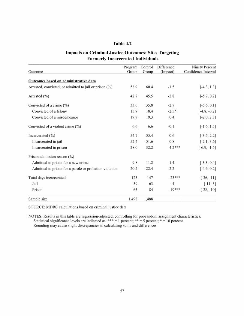
57
Table 4.2
Impacts on Criminal Justice Outcomes: Sites Targeting Formerly Incarcerated Individuals
Program Control Difference Ninety Percent Outcome Group Group (Impact) Confidence Interval
Outcomes based on administrative data Arrested, convicted, or admitted to jail or prison (%) 58.9 60.4 -1.5 [-4.3, 1.3]
Arrested (%) 42.7 45.5 -2.8 [-5.7, 0.2]
Convicted of a crime (%) 33.0 35.8 -2.7 [-5.6, 0.1] Convicted of a felony 15.9 18.4 -2.5 * [-4.8, -0.2] Convicted of a misdemeanor 19.7 19.3 0.4 [-2.0, 2.8]
Convicted of a violent crime (%) 6.6 6.6 -0.1 [-1.6, 1.5]
Incarcerated (%) 54.7 55.4 -0.6 [-3.5, 2.2] Incarcerated in jail 52.4 51.6 0.8 [-2.1, 3.6] Incarcerated in prison 28.0 32.2 -4.2 *** [-6.9, -1.6]
Prison admission reason (%)
Admitted to prison for a new crime 9.8 11.2 -1.4 [-3.3, 0.4] Admitted to prison for a parole or probation violation 20.2 22.4 -2.2 [-4.6, 0.2]
Total days incarcerated 123 147 -23 *** [-36, -11] Jail 59 63 -4 [-11, 3] Prison 65 84 -19 *** [-28, -10]
Sample size 1,498 1,488 SOURCE: MDRC calculations based on criminal justice data. NOTES: Results in this table are regression-adjusted, controlling for pre-random assignment characteristics. Statistical significance levels are indicated as: *** = 1 percent; ** = 5 percent; * = 10 percent. Rounding may cause slight discrepancies in calculating sums and differences.
58
Figure 4.1 presents impacts on having a criminal justice event during the 30-month fol-low-up period, for each site separately. The Indianapolis program reduced this broad measure of recidivism by about 6 percentage points: 67 percent of the program group had a criminal justice event compared with 74 percent of the control group. There was no statistically significant reduc-tion in recidivism in Fort Worth, and the New York City program led to a small increase in this measure of recidivism. The difference in impacts among sites is statistically significant.3
One theory of transitional jobs programs for formerly incarcerated people is that partici-pation in program services, including subsidized employment, may keep people active and away from situations that would lead to additional contact with the criminal justice system.4 If this theory were true, then programs with an emphasis on rapid engagement and high levels of partic-ipation should be more successful at reducing recidivism. As shown in Figure 1.2 of this report (and described in the ETJD interim report),5 Indianapolis had the highest rate of participation in subsidized employment among the three programs targeting formerly incarcerated people (100 percent of program group members worked in subsidized jobs versus 79 percent of program group members in New York City and 39 percent in Fort Worth) and put participants to work the quickest.6 As described in more detail in the ETJD interim report, the Indianapolis program also featured peer mentoring for all participants and a daily “Circle of Trust” wherein participants collectively shared and discussed experiences and solutions to challenges they faced. It is possible that these features contributed to stronger interpersonal ties and feelings of community that also could have resulted in reduced recidivism.
Another factor in interpreting the differences in the impacts among programs is that in New York City, the control group had access to another program that offered services similar to those provided by the ETJD program (including subsidized employment). This program, the Cen-ter for Employment Opportunities (CEO), is a large not-for-profit organization previously shown to be effective at reducing recidivism in a rigorous random assignment study.7 As shown earlier in this report, the impact on services received by program group members compared with control
3The p-value for this test of differences in impacts among sites is p = 0.017. 4Redcross, Millenky, Rudd, and Levshin (2012). 5Redcross et al. (2016). 6It is important to note that some earlier programs with high levels of participation in transitional jobs did
not reduce recidivism. For example, in the Transitional Jobs Reentry Demonstration, in three of the four pro-grams studied, program group member participation in transitional jobs was 87 percent or higher, with none of these three programs producing a statistically significant reduction in recidivism at the end of a two-year follow-up period. Conversely, the Center for Employment Opportunities, a transitional jobs program that produced sig-nificant reductions in recidivism, had a transitional jobs participation rate of about 71 percent. See Redcross et al. (2010), Jacobs (2012), and Redcross et al. (2012).
7Redcross et al. (2012).
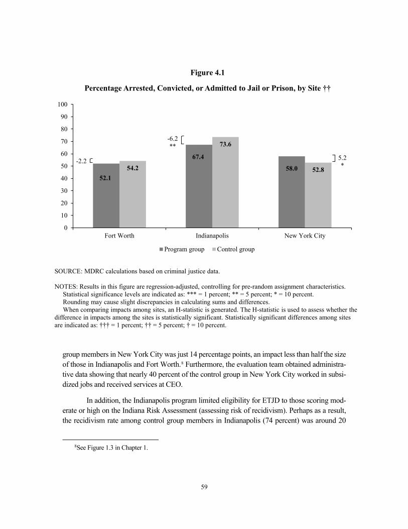
59
Figure 4.1
Percentage Arrested, Convicted, or Admitted to Jail or Prison, by Site ††
-2.2
-6.2**
5.2*
52.1
67.4
58.054.2
73.6
52.8
0
10
20
30
40
50
60
70
80
90
100
Fort Worth Indianapolis New York City
Program group Control group
SOURCE: MDRC calculations based on criminal justice data.
NOTES: Results in this figure are regression-adjusted, controlling for pre-random assignment characteristics. Statistical significance levels are indicated as: *** = 1 percent; ** = 5 percent; * = 10 percent.Rounding may cause slight discrepancies in calculating sums and differences.When comparing impacts among sites, an H-statistic is generated. The H-statistic is used to assess whether the
difference in impacts among the sites is statistically significant. Statistically significant differences among sites are indicated as: ††† = 1 percent; †† = 5 percent; † = 10 percent.
group members in New York City was just 14 percentage points, an impact less than half the size of those in Indianapolis and Fort Worth.8 Furthermore, the evaluation team obtained administra-tive data showing that nearly 40 percent of the control group in New York City worked in subsi-dized jobs and received services at CEO.
In addition, the Indianapolis program limited eligibility for ETJD to those scoring mod-erate or high on the Indiana Risk Assessment (assessing risk of recidivism). Perhaps as a result, the recidivism rate among control group members in Indianapolis (74 percent) was around 20
8See Figure 1.3 in Chapter 1.
60
percentage points higher than that of control group members in New York City (53 percent) or Fort Worth (54 percent).9 Previous studies of prisoner reentry programs — including the study of the CEO program mentioned earlier in this section — have demonstrated that intensive services like transitional jobs are most beneficial for people at higher risk of recidivism.10 The fact that the Indianapolis ETJD program had high rates of program participation, successfully implemented its model,11 and served a higher-risk population may have contributed to its positive impacts on recidivism.
● The Indianapolis ETJD program reduced arrests, prison admissions, and the number of days incarcerated in prison. The other two programs that targeted formerly incarcerated people did not produce consistent impacts on these outcomes.
To further explore the site-level story described in the previous section, Table 4.3 presents ETJD’s impacts on exploratory measures of recidivism for each site separately. As shown in the table, the Indianapolis program led to statistically significant reductions in arrests, prison admis-sions, and the number of days incarcerated in prison. Recidivism was relatively high for both research groups in Indianapolis: More than 73 percent of the control group was arrested over the 30-month follow-up period, compared with 67 percent of the program group. The other sections of Table 4.3 show that there were no significant impacts on criminal justice outcomes in Fort Worth, and impacts in New York City were inconsistent (increases in arrests and incarceration in jail and reductions in prison admissions). The righthand column of Table 4.3 shows daggers in-dicating which of the differences in impacts among sites is statistically significant, with one dag-ger indicating significance at the 10 percent level, two daggers indicating significance at the 5
9Although the Fort Worth and New York City programs also set additional eligibility criteria for entry into
ETJD beyond those required by the U.S. Department of Labor, these criteria were either broad (in the case of the Fort Worth program) or designed to target those who were somewhat ready to work (in the case of the New York City program). See Chapters 6 and 8 of this study’s interim report (Redcross et al., 2016) for more details on these eligibility requirements. The differences in control group recidivism rates could also be due to Indianapolis’ overall criminal justice environment. For example, Indianapolis may police more heavily and police officers there may be more likely to make arrests than police officers in Fort Worth or New York City, or parole officers may supervise parolees more intensely or be more likely to cite them for violations. But regardless of the cause, the end result is that ETJD population in Indianapolis was at a higher risk of having an interaction with the criminal justice system.
10Zweig, Yahner, and Redcross (2010); Latessa (2008). 11All participants received services and worked in transitional jobs, but certain components of the model
were not well implemented at RecycleForce’s partner organizations, which together served around 25 percent of ETJD participants in Indianapolis. Some of those participants ultimately received the services through Recycle-Force. See Redcross et al. (2016).
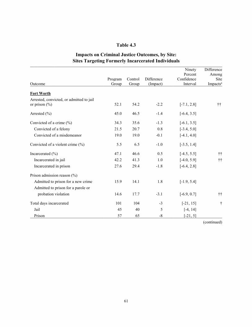
61
Table 4.3
Impacts on Criminal Justice Outcomes, by Site: Sites Targeting Formerly Incarcerated Individuals
(continued)
Ninety Difference Percent Among
Program Control Difference Confidence Site Outcome Group Group (Impact) Interval Impactsa
Fort Worth Arrested, convicted, or admitted to jail or prison (%) 52.1 54.2 -2.2 [-7.1, 2.8] ††
Arrested (%) 45.0 46.5 -1.4 [-6.4, 3.5]
Convicted of a crime (%) 34.3 35.6 -1.3 [-6.1, 3.5] Convicted of a felony 21.5 20.7 0.8 [-3.4, 5.0] Convicted of a misdemeanor 19.0 19.0 -0.1 [-4.1, 4.0]
Convicted of a violent crime (%) 5.5 6.5 -1.0 [-3.5, 1.4]
Incarcerated (%) 47.1 46.6 0.5 [-4.5, 5.5] †† Incarcerated in jail 42.2 41.3 1.0 [-4.0, 5.9] †† Incarcerated in prison 27.6 29.4 -1.8 [-6.4, 2.8]
Prison admission reason (%) Admitted to prison for a new crime 15.9 14.1 1.8 [-1.9, 5.4] Admitted to prison for a parole or
probation violation 14.6 17.7 -3.1 [-6.9, 0.7] ††
Total days incarcerated 101 104 -3 [-21, 15] † Jail 45 40 5 [-4, 14] Prison 57 65 -8 [-21, 5]
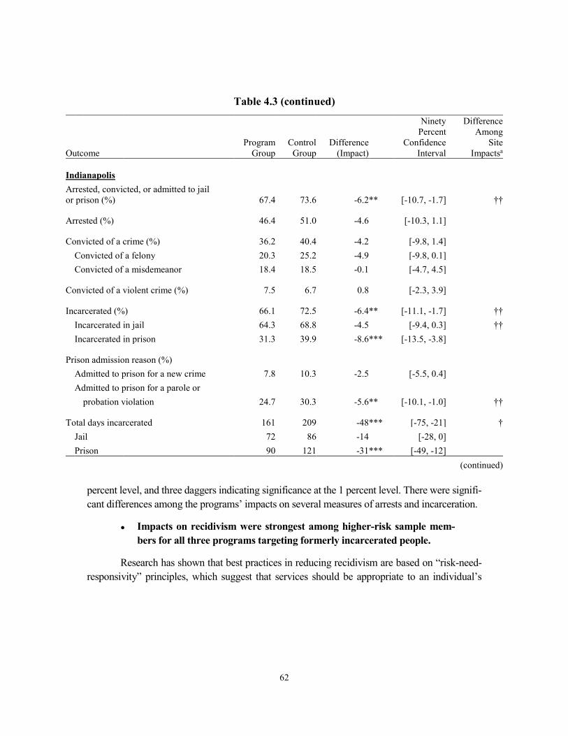
62
Table 4.3 (continued) Ninety Difference Percent Among Program Control Difference Confidence Site
Outcome Group Group (Impact) Interval Impactsa Indianapolis Arrested, convicted, or admitted to jail or prison (%) 67.4 73.6 -6.2 ** [-10.7, -1.7] ††
Arrested (%) 46.4 51.0 -4.6 [-10.3, 1.1]
Convicted of a crime (%) 36.2 40.4 -4.2 [-9.8, 1.4] Convicted of a felony 20.3 25.2 -4.9 [-9.8, 0.1] Convicted of a misdemeanor 18.4 18.5 -0.1 [-4.7, 4.5]
Convicted of a violent crime (%) 7.5 6.7 0.8 [-2.3, 3.9]
Incarcerated (%) 66.1 72.5 -6.4 ** [-11.1, -1.7] †† Incarcerated in jail 64.3 68.8 -4.5 [-9.4, 0.3] †† Incarcerated in prison 31.3 39.9 -8.6 *** [-13.5, -3.8]
Prison admission reason (%) Admitted to prison for a new crime 7.8 10.3 -2.5 [-5.5, 0.4] Admitted to prison for a parole or
probation violation 24.7 30.3 -5.6 ** [-10.1, -1.0] ††
Total days incarcerated 161 209 -48 *** [-75, -21] † Jail 72 86 -14 [-28, 0] Prison 90 121 -31 *** [-49, -12] (continued)
percent level, and three daggers indicating significance at the 1 percent level. There were signifi-cant differences among the programs’ impacts on several measures of arrests and incarceration.
● Impacts on recidivism were strongest among higher-risk sample mem-bers for all three programs targeting formerly incarcerated people.
Research has shown that best practices in reducing recidivism are based on “risk-need-responsivity” principles, which suggest that services should be appropriate to an individual’s
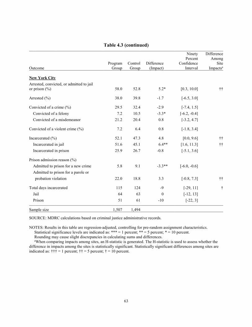
63
Table 4.3 (continued) Ninety Difference Percent Among Program Control Difference Confidence Site
Outcome Group Group (Impact) Interval Impactsa New York City Arrested, convicted, or admitted to jail or prison (%) 58.0 52.8 5.2 * [0.3, 10.0] ††
Arrested (%) 38.0 39.8 -1.7 [-6.5, 3.0]
Convicted of a crime (%) 29.5 32.4 -2.9 [-7.4, 1.5] Convicted of a felony 7.2 10.5 -3.3 * [-6.2, -0.4] Convicted of a misdemeanor 21.2 20.4 0.8 [-3.2, 4.7]
Convicted of a violent crime (%) 7.2 6.4 0.8 [-1.8, 3.4]
Incarcerated (%) 52.1 47.3 4.8 [0.0, 9.6] †† Incarcerated in jail 51.6 45.1 6.4 ** [1.6, 11.3] †† Incarcerated in prison 25.9 26.7 -0.8 [-5.1, 3.6]
Prison admission reason (%) Admitted to prison for a new crime 5.8 9.1 -3.3 ** [-6.0, -0.6] Admitted to prison for a parole or probation violation 22.0 18.8 3.3 [-0.8, 7.3] ††
Total days incarcerated 115 124 -9 [-29, 11] † Jail 64 63 0 [-12, 13] Prison 51 61 -10 [-22, 3]
Sample size 1,507 1,494 SOURCE: MDRC calculations based on criminal justice administrative records. NOTES: Results in this table are regression-adjusted, controlling for pre-random assignment characteristics. Statistical significance levels are indicated as: *** = 1 percent; ** = 5 percent; * = 10 percent. Rounding may cause slight discrepancies in calculating sums and differences. aWhen comparing impacts among sites, an H-statistic is generated. The H-statistic is used to assess whether the difference in impacts among the sites is statistically significant. Statistically significant differences among sites are indicated as: ††† = 1 percent; †† = 5 percent; † = 10 percent.
64
needs and risk of recidivism.12 Specifically, intensive services should not be provided to people at low risk of recidivism; instead they should be reserved for people assessed to be at higher risk of recidivism using validated risk-assessment tools. As noted earlier, previous rigorous research supports these risk-need-responsivity guidelines and has found that transitional jobs programs can be more effective at reducing recidivism among those who are at a higher risk of recidivism.13 To test this theory, a subgroup analysis was conducted to assess whether the ETJD programs target-ing formerly incarcerated people had different effects on criminal justice outcomes for partici-pants at higher and lower risk for reoffending.14 Table 4.4 shows that reductions in recidivism were concentrated among those at higher risk, and that impacts on criminal justice measures dif-fered significantly between those at higher risk and lower risk. Higher-risk program group mem-bers were 12 percentage points less likely to be incarcerated in prison than higher-risk control group members, while there was no statistically significant difference in rates of incarceration in prison between lower-risk program and control group members.
It is important to note that the sample in Indianapolis may be dominating the sample from the other two sites in this pooled analysis because Indianapolis served more high-risk individuals. Thus, site-specific subgroup analysis based on risk may be more informative regarding ETJD’s effects for those at higher and lower risk of recidivism. Appendix Tables F.3, G.3, and H.3 present site-specific impact results for these subgroups at each of the sites separately. The findings con-firm that the impacts on certain measures of recidivism are somewhat stronger among those at highest risk at each of the sites. In general, ETJD’s findings are consistent with previous research showing that intensive transitional jobs program services can reduce recidivism for those at the highest risk of recidivism.
Impacts on criminal justice outcomes were also examined for subgroups based on age, education, and time of entering the study. As shown in Appendix A, there are no statistically significant differences in impacts for any of these subgroups.
12Petersilia (2004); Solomon et al. (2008). 13Zweig, Yahner, and Redcross (2010). 14See Appendix L for a discussion of the methods used to determine risk of reoffending.
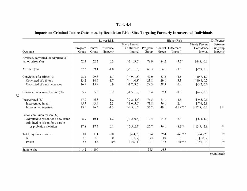
Table 4.4
Impacts on Criminal Justice Outcomes, by Recidivism Risk: Sites Targeting Formerly Incarcerated Individuals
(continued)
Lower Risk Higher Risk Difference
Ninety Percent Ninety Percent Between Program Control Difference Confidence Program Control Difference Confidence Subgroup
Outcome Group Group (Impact) Interval Group Group (Impact) Interval Impactsa
Arrested, convicted, or admitted to jail or prison (%) 52.4 52.2 0.3 [-3.1, 3.6] 78.9 84.2 -5.2 * [-9.8, -0.6]
Arrested (%) 37.3 39.1 -1.8 [-5.1, 1.6] 60.3 64.1 -3.8 [-9.9, 2.3]
Convicted of a crime (%) 28.1 29.8 -1.7 [-4.9, 1.5] 49.0 53.5 -4.5 [-10.7, 1.7] Convicted of a felony 13.2 14.9 -1.7 [-4.1, 0.8] 23.8 29.1 -5.3 [-10.8, 0.2] Convicted of a misdemeanor 16.9 15.9 0.9 [-1.7, 3.6] 29.3 28.9 0.4 [-5.2, 6.0]
Convicted of a violent crime (%) 5.9 5.8 0.2 [-1.5, 1.9] 8.4 9.3 -0.9 [-4.5, 2.7]
Incarcerated (%) 47.9 46.8 1.2 [-2.2, 4.6] 76.5 81.1 -4.5 [-9.5, 0.5] Incarcerated in jail 45.7 43.4 2.3 [-1.0, 5.6] 73.8 76.1 -2.4 [-7.6, 2.9] Incarcerated in prison 25.0 26.5 -1.5 [-4.5, 1.5] 37.2 49.1 -11.9 *** [-17.8, -6.0] †††
Prison admission reason (%) Admitted to prison for a new crime 8.9 10.1 -1.2 [-3.2, 0.8] 12.4 14.8 -2.4 [-6.4, 1.7] Admitted to prison for a parole or probation violation 17.8 17.7 0.1 [-2.5, 2.7] 27.7 36.1 -8.3 ** [-13.9, -2.8] ††
Total days incarcerated 101 111 -10 [-24, 3] 194 254 -60 *** [-94, -27] †† Jail 48 48 0 [-7, 7] 94 110 -16 [-34, 2] Prison 53 63 -10 * [-19, -1] 101 142 -41 *** [-64, -19] ††
Sample size 1,142 1,109 365 385
65

66
Table 4.4 (continued) SOURCE: MDRC calculations based on criminal justice administrative records. NOTES: Results in this table are regression-adjusted, controlling for pre-random assignment characteris-tics. Statistical significance levels are indicated as: *** = 1 percent; ** = 5 percent; * = 10 percent. Rounding may cause slight discrepancies in calculating sums and differences. See Appendix L for details on how risk of recidivism was defined. aWhen comparing impacts between two subgroups, an H-statistic is generated. The H-statistic is used to assess whether the difference in impacts between the subgroups is statistically significant. Statistically sig-nificant differences between subgroups are indicated as: ††† = 1 percent; †† = 5 percent; † = 10 percent.

67
Chapter 5
Cost Analysis
This chapter presents estimates of the costs of operating the Enhanced Transitional Jobs Demonstration (ETJD) programs and the costs of services that program group and control group members received outside of the ETJD programs. The net cost of ETJD programs provides an estimate of how much more was spent on program group members than control group mem-bers. The chapter begins with a brief description of the method used in the cost analysis. It concludes with a comparison between net costs and important outcomes.
Method The cost analysis compares the expenditures for serving the program group with expenditures for serving the control group. These are one-year cost estimates, reflecting service participation sample members reported in the survey administered 12 months after random assignment. Most of the program group services presented in this chapter were funded by the Department of Labor ETJD grant, though other sources may have funded some of the non-ETJD services. All costs have been adjusted to 2016 dollars for this analysis.
Main Components of the Cost Analysis
Figure 5.1 depicts the main cost components for both the program and control groups. It shows that the total cost for each program group member (Box C) is made up of ETJD program costs (Box A) and expenditures for services received outside of ETJD (Box B). Box E repre-sents the total cost that accrued for each control group member. The net cost of ETJD (Box F) is the cost per program group member over and above the cost per control group member.
ETJD Program Costs (Box A)
To estimate the ETJD program costs, the evaluation team collected expenditure reports from each program. A period was selected approximately one year after the program began operations to avoid including costs associated with start-up activities and to include a period when the program was operating at full capacity.1 ETJD expenditures were divided into the costs of operations, the support services, and the subsidized wages.
1Each program received between $5.6 million and $5.7 million and was expected to serve at least 500
participants. However, the per-person cost for ETJD is less than the total grant divided by the number of participants served for several reasons. First, efforts were made to exclude research-related expenses (that is,
(continued)

68
●
●
●
Operating costs included all staff salaries, fringe benefits, overhead, admin-istrative costs, and payroll costs, including payroll taxes and workers’ com-pensation. Some ETJD programs paid other organizations to provide services such as education, training, legal services, and counseling services, and these costs are included in this category.
Support services were provided to participants to help them attend the pro-gram and work at their jobs. For example, most programs provided partici-pants with bus passes or reimbursed them for other transportation costs. Many programs reimbursed participants for work-related expenses (for ex-ample, the cost of work uniforms and tools) and some gave participants in-centive payments to encourage them to participate in the program or meet program milestones.
Wages were the subsidized wages and fringe benefits paid to program group members.
To estimate the cost of program operations and support services, the analysis calculated an average monthly cost per program group member. This monthly cost was multiplied by the average number of months that participants spent in ETJD over the year following random assignment. Data on the average subsidized wages came from administrative records provided to the research team.
Non-ETJD Costs (Boxes B and D)
ETJD programs may encourage participants to receive outside services. For example, some may make referrals to education and training services paid for by school districts, com-munity colleges, or American Job Centers funded by the Workforce Innovation and Opportuni-ty Act. In addition, some program group members sought out services on their own.
The cost of services provided to control group members represents what government entities at all levels would have spent on program group members in the absence of the ETJD
expenses required to accommodate research requirements and requests). Second, some grant funding was used during the six-month planning period before the program began operating. Third, the period selected for the cost analysis was a period in which the programs were operating at full capacity. During the period selected they were able to operate more efficiently than they were in the early period when they were recruiting participants, or than they were in the last year of the grant when they were no longer enrolling new participants. Finally, the costs reflect services provided to participants over the first year of their involvement, and some participants may have stayed in the program for longer than one year.
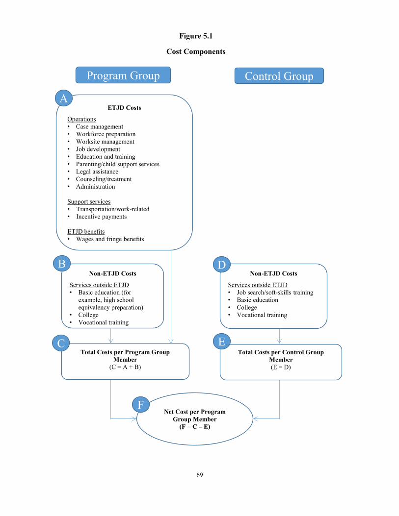
69
Cost Components
Figure 5.1
Non-ETJD Costs
Services outside ETJD• Job search/soft-skills training• Basic education• College• Vocational training
ETJD Costs
Operations• Case management• Workforce preparation• Worksite management• Job development• Education and training• Parenting/child support services• Legal assistance• Counseling/treatment• Administration
Support services• Transportation/work-related• Incentive payments
ETJD benefits• Wages and fringe benefits
Program Group Control Group
A
Non-ETJD Costs
Services outside ETJD• Basic education (for
example, high school equivalency preparation)
• College• Vocational training
B
Total Costs per Program Group Member
(C = A + B)
CTotal Costs per Control Group
Member (E = D)
E
Net Cost per Program Group Member
(F = C – E)
F
D

70
programs. The cost components for the control group consist of expenditures by outside agencies for providing job-search services, education, training, and in some cases transitional jobs).
Information on the extent to which program group and control group members made use of non-ETJD services comes from the participant survey administered 12 months after random assignment. The survey asked respondents to estimate the number of weeks they spent in the following activities. Weekly unit costs (the estimated costs of serving one person for one week) were constructed for each of these activities based on information available from pub-lished sources.
●
●
●
●
Job-search, job-readiness, and career-planning services included receiv-ing help with job searching, job referrals, developing a résumé, filling out job applications, preparing for job interviews, job-readiness training, and plan-ning for future career or educational goals. Cost estimates came from a na-tional study of WIA Adult and Dislocated Worker programs.2
Basic education included participation in English as a Second Language classes, adult basic education classes, classes to prepare for a high school diploma, and high school equivalency classes, including those leading to a General Educational Development (GED) certificate. Basic education costs were calculated by state using data from the U.S. Department of Education’s Office of Career, Technical, and Adult Education’s National Reporting System.
College included attending courses at community, two-year, and four-year colleges. Costs were estimated using data from the U.S. Department of Edu-cation’s National Center for Education Statistics’ Integrated Postsecondary Education Data System (IPEDS).
Vocational training included training for a specific job, trade, or occupation. Survey respondents named the training provider where they received the training and a cost was applied based on the type of institution that provided the training (for example, private school, adult school, or community college).3
2Mastri and McCutcheon (2015). 3The cost of private-school training was estimated using data from IPEDS on the cost of for-profit provid-
ers offering the types of training that sample group members may have taken during this period (based on information gathered during site visits). These types included trucking, automotive, welding, maintenance, cosmetology, culinary, and heating, ventilation, and air conditioning (HVAC) training. Data on the cost of
(continued)
71
In addition to the job-search, education, and training costs, at two sites (New York City and Milwaukee), control group members participated in subsidized employment offered by other programs available in the community. In New York City, data show that around 16 percent of program group members and 36 percent of control group members received subsi-dized jobs from the Center for Employment Opportunities (CEO), a nonprofit organization in New York City. These subsidized wages and associated program costs are included in New York City’s non-ETJD costs.4 In Milwaukee, the state of Wisconsin operated a program called the Transitional Jobs Demonstration Project from September 2010 to June 2013, and the city operated a program called the Transform Milwaukee Jobs Program in 2014. About 19 percent of program group members and 22 percent of control group members received subsidized jobs through these programs. The costs of these other programs are not included in the Milwaukee analysis because the program and control group participation rates were nearly the same.
Limitations of the Analysis
The cost analysis has several limitations worth noting. First, with the exception of par-ticipation in job searching and vocational training, the survey did not ask where participants received services nor the types of institutions that they attended. The analysis assumed that participants received basic education at adult schools and college instruction at community colleges.
As noted above, for the job-search component, the analysis used estimates from a na-tional study of the public workforce system’s Adult and Dislocated Worker programs to estimate the cost of services received by the control group. Because program group members received job-search assistance from the ETJD programs, an assumption was made that they did not receive additional services outside of the ETJD programs. Additionally, the cost obtained from the national study reflects a range of job-search services, and it is not known which services control group members received, nor the number of times they received those services in a given week. The analysis took the average cost of the full range of job-search services reported in the national study and applied it to an estimate of the average number of weeks control group members received the services.5
adult schools came from the U.S. Department of Education’s Office of Career, Technical, and Adult Educa-tion’s National Reporting System and data on the cost of community colleges came from IPEDS. Note that some reported training was provided by the employer or paid for by the ETJD program; no cost estimate was applied to either type (though ETJD training was included in the ETJD cost estimates).
4CEO matched its subsidized wage payroll data with ETJD sample member information. Program costs were estimated using data from an earlier cost analysis of CEO (Redcross et al., 2009).
5The per-person cost estimates from Mastri and McCutcheon (2015) were $16 for a resource-room visit, $13 for a structured assessment, $38 for a job-club meeting, $54 for a workshop, and $143 for a one-on-one
(continued)
72
ETJD Costs As described above, the costs of providing ETJD program services are divided into three categories: (1) the operating costs of the ETJD program, which includes all staff salaries, fringe benefits, overhead, administrative costs, and payroll costs; (2) the support services provided to program group members; and (3) the subsidized wages.
As shown in Table 5.1, the costs of providing ETJD services ranges from about $7,000 in Milwaukee to about $11,100 in Indianapolis. Note that the Indianapolis program’s operating expenses were substantially higher than those of programs in other cities, as they included some of the costs of running RecycleForce, a social-enterprise business that brought in revenue from recycling sales.6 The total cost, taking that revenue into account, is about $7,800, which is equivalent to the other ETJD programs’ costs.
While the estimated ETJD cost per person did not differ substantially across programs (after taking revenue into account in Indianapolis), some programs spent more on operations while others spent more on support services or wages. For example, the cost of operations ranged from a low of about $3,600 in Atlanta to a high of $6,600 in Fort Worth.
Support-service costs ranged from about $120 in Milwaukee to close to $1,000 in San Francisco. The programs that had higher support-service costs (those in Fort Worth, New York City, and San Francisco) provided incentive payments or stipends to participants who attended program activities, obtained employment, or maintained employment.
The wages shown are those paid to participants or, in some cases, paid to employers to reimburse them for the wages they paid to participants. The wages ranged from about $1,100 in Fort Worth (where relatively few program group members worked in transitional jobs) and $1,200 in New York City (where participants only worked part time), to about $4,600 in Indianapolis (where all program group members worked and many were allowed to stay in subsidized jobs for longer than planned).
counselor meeting. The average of $53 (or $55 in 2016 dollars) was applied to the estimated number of weeks that control group members received job-search services.
6For more information on RecycleForce and the Indianapolis ETJD program’s implementation, see Red-cross et al. (2016), Chapter 7. For more information on the costs of RecycleForce, see Foley, Farrell, Webster, and Walter (forthcoming).
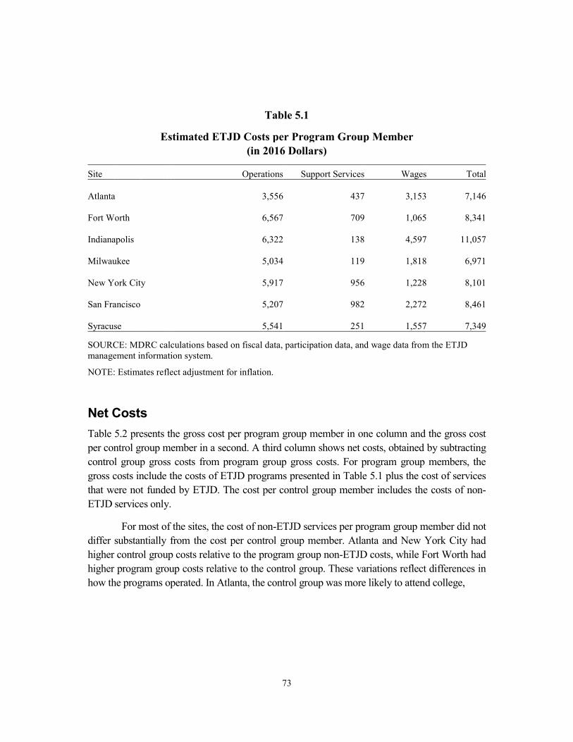
73
Table 5.1
Estimated ETJD Costs per Program Group Member (in 2016 Dollars)
Site
Operations Support Services Wages Total
Atlanta 3,556 437 3,153 7,146
Fort Worth 6,567 709 1,065 8,341
Indianapolis 6,322 138 4,597 11,057
Milwaukee 5,034 119 1,818 6,971
New York City 5,917 956 1,228 8,101
San Francisco 5,207 982 2,272 8,461
Syracuse 5,541 251 1,557 7,349
SOURCE: MDRC calculations based on fiscal data, participation data, and wage data from the ETJD management information system.
NOTE: Estimates reflect adjustment for inflation.
Net Costs Table 5.2 presents the gross cost per program group member in one column and the gross cost per control group member in a second. A third column shows net costs, obtained by subtracting control group gross costs from program group gross costs. For program group members, the gross costs include the costs of ETJD programs presented in Table 5.1 plus the cost of services that were not funded by ETJD. The cost per control group member includes the costs of non-ETJD services only.
For most of the sites, the cost of non-ETJD services per program group member did not differ substantially from the cost per control group member. Atlanta and New York City had higher control group costs relative to the program group non-ETJD costs, while Fort Worth had higher program group costs relative to the control group. These variations reflect differences in how the programs operated. In Atlanta, the control group was more likely to attend college,
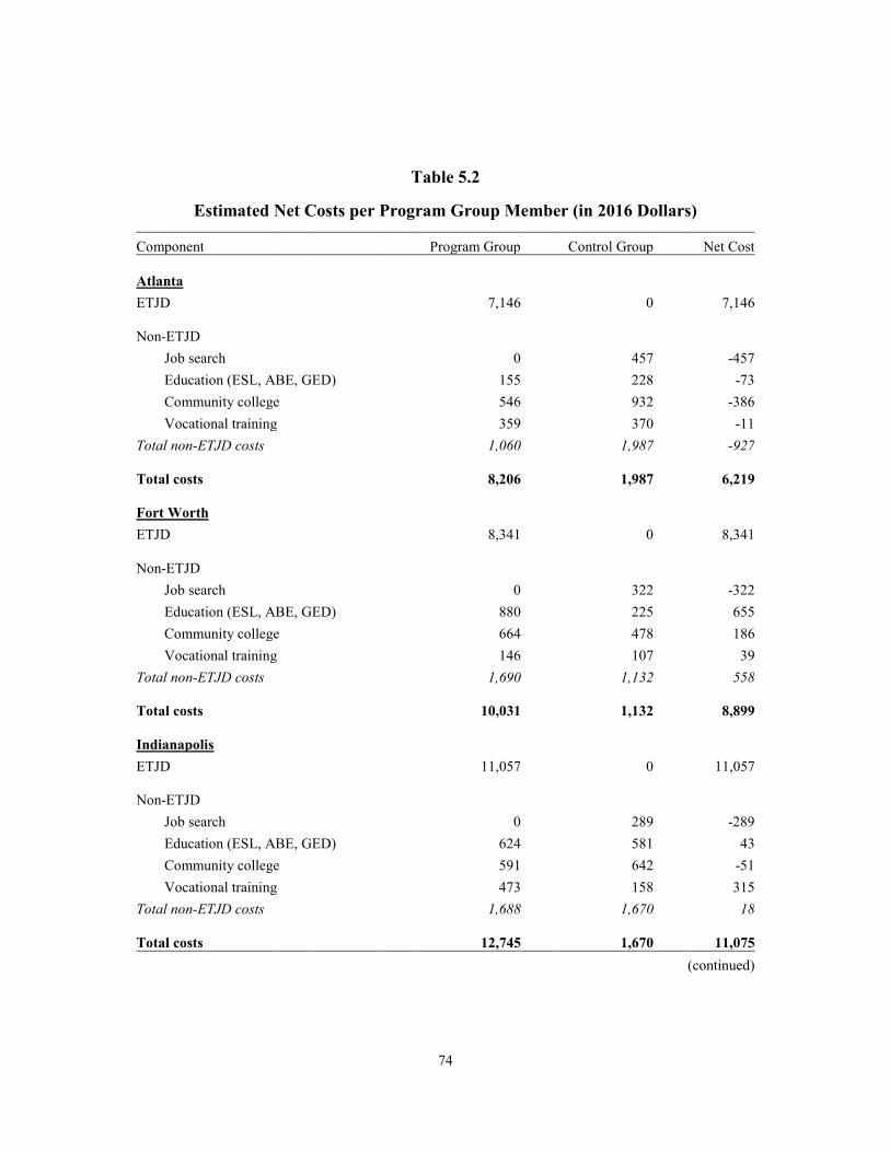
74
Table 5.2
Estimated Net Costs per Program Group Member (in 2016 Dollars)
(continued)
Component Program Group Control Group Net Cost
Atlanta ETJD 7,146 0 7,146
Non-ETJD
Job search 0 457 -457 Education (ESL, ABE, GED) 155 228 -73 Community college 546 932 -386 Vocational training 359 370 -11
Total non-ETJD costs 1,060 1,987 -927
Total costs 8,206 1,987 6,219
Fort Worth ETJD 8,341 0 8,341
Non-ETJD Job search 0 322 -322
Education (ESL, ABE, GED) 880 225 655 Community college 664 478 186 Vocational training 146 107 39
Total non-ETJD costs 1,690 1,132 558
Total costs 10,031 1,132 8,899
Indianapolis ETJD 11,057 0 11,057
Non-ETJD Job search 0 289 -289
Education (ESL, ABE, GED) 624 581 43 Community college 591 642 -51 Vocational training 473 158 315
Total non-ETJD costs 1,688 1,670 18
Total costs 12,745 1,670 11,075
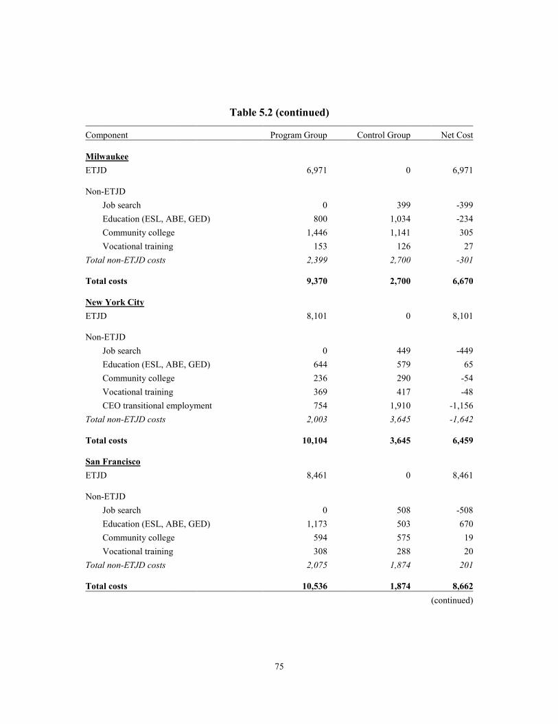
75
(continued)
Table 5.2 (continued)
Component Program Group Control Group Net Cost
Milwaukee ETJD
J
6,971 0 6,971
Non-ETJD ob search 0 399 -399
Education (ESL, ABE, GED) 800 1,034 -234 Community college 1,446 1,141 305 Vocational training 153 126 27
Total non-ETJD costs 2,399 2,700 -301
Total costs 9,370 2,700 6,670
New York City ETJD 8,101 0 8,101
Non-ETJD Job search 0 449 -449
Education (ESL, ABE, GED) 644 579 65 Community college 236 290 -54 Vocational training 369 417 -48 CEO transitional employment 754 1,910 -1,156
Total non-ETJD costs 2,003 3,645 -1,642
Total costs 10,104 3,645 6,459
San Francisco ETJD 8,461 0 8,461
Non-ETJD Job search 0 508 -508
Education (ESL, ABE, GED) 1,173 503 670 Community college 594 575 19 Vocational training 308 288 20
Total non-ETJD costs 2,075 1,874 201
Total costs 10,536 1,874 8,662
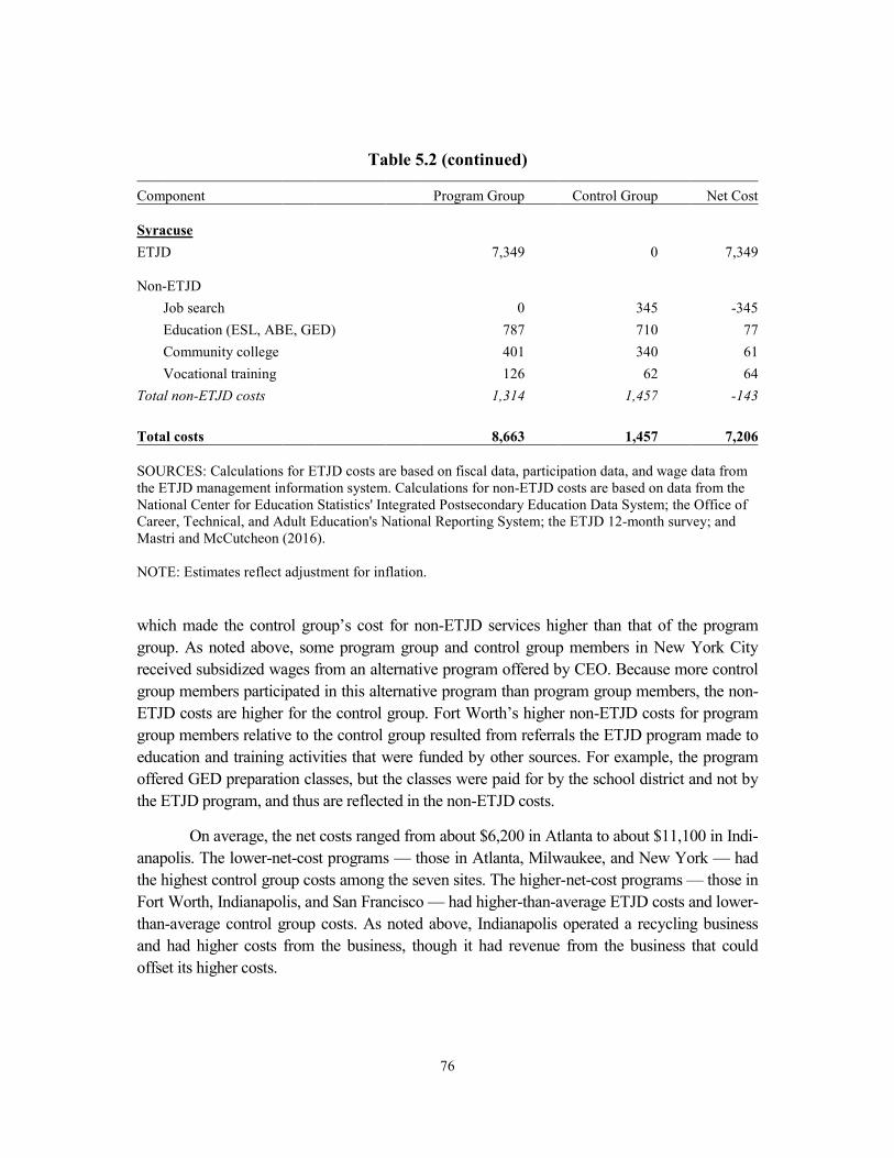
76
Table 5.2 (continued)
Component Program Group Control Group Net Cost
Syracuse ETJD
7,349 0 7,349
Non-ETJD Job search 0 345 -345
Education (ESL, ABE, GED) 787 710 77 Community college 401 340 61 Vocational training 126 62 64
Total non-ETJD costs 1,314 1,457 -143
Total costs 8,663 1,457 7,206
SOURCES: Calculations for ETJD costs are based on fiscal data, participation data, and wage data from the ETJD management information system. Calculations for non-ETJD costs are based on data from the National Center for Education Statistics' Integrated Postsecondary Education Data System; the Office of Career, Technical, and Adult Education's National Reporting System; the ETJD 12-month survey; and Mastri and McCutcheon (2016). NOTE: Estimates reflect adjustment for inflation.
which made the control group’s cost for non-ETJD services higher than that of the program group. As noted above, some program group and control group members in New York City received subsidized wages from an alternative program offered by CEO. Because more control group members participated in this alternative program than program group members, the non- ETJD costs are higher for the control group. Fort Worth’s higher non-ETJD costs for program group members relative to the control group resulted from referrals the ETJD program made to education and training activities that were funded by other sources. For example, the program offered GED preparation classes, but the classes were paid for by the school district and not by the ETJD program, and thus are reflected in the non-ETJD costs.
On average, the net costs ranged from about $6,200 in Atlanta to about $11,100 in Indi-anapolis. The lower-net-cost programs — those in Atlanta, Milwaukee, and New York — had the highest control group costs among the seven sites. The higher-net-cost programs — those in Fort Worth, Indianapolis, and San Francisco — had higher-than-average ETJD costs and lower-than-average control group costs. As noted above, Indianapolis operated a recycling business and had higher costs from the business, though it had revenue from the business that could offset its higher costs.
77
Was ETJD Cost-Effective? There are several approaches that could be used to assess whether ETJD was cost-effective. A simple cost-effectiveness analysis examines the relative costs of achieving the same outcome, typically a nonmonetary outcome, across similar programs. This type of analysis can help administrators assess whether a particular program is less or more cost-effective in delivering the same outcome than others. A limitation of this type of analysis is that it assumes that the programs are primarily interested in affecting one outcome. As outlined in Chapter 1, ETJD sought to affect multiple outcomes. All ETJD programs sought to increase earnings, but the four ETJD programs targeting noncustodial parents also sought to increase child support payments, and the three ETJD programs targeting formerly incarcerated individuals sought to reduce recidivism.
Another approach to assess a program’s cost-effectiveness is to conduct a benefit-cost analysis. This approach provides an overall accounting of the financial gains and losses pro-duced by the program from the perspectives of the participants, the government, and society. A full benefit-cost analysis examines additional measures that go beyond the measures presented in this report, including the potential savings associated with recidivism and the costs and benefits associated with increased earnings, including effects on taxes and fringe benefits. A companion document presents the results of a benefit-cost analysis of the ETJD program in Indianapolis.7
A simpler approach is to compare the net costs with the main outcomes affected by the program. Table 5.3 shows the net costs for each program alongside the impacts on the confirma-tory outcomes over the full follow-up period available (approximately three years for earnings and child support payments and 30 months for criminal justice events). In addition, it shows impacts on child support after 12 months for the three programs targeting formerly incarcerated individuals and impacts on the broad measure of recidivism after 12 months for the four programs targeting noncustodial parents. (These exploratory analyses are presented in italics and shaded.)8
At all sites, the net cost per person exceeded the increase in earnings. Among the four programs targeting noncustodial parents, those in Atlanta and Milwaukee produced statistically significant impacts on child support payments over three years and the Atlanta program reduced recidivism in the first year. Among the programs targeting people returning home from prison, the one in Indianapolis produced a reduction in recidivism over 30 months and an increase in
7Foley, Farrell, Webster, and Walter (forthcoming). 8Impacts on recidivism were not measured beyond 12 months at the sites targeting noncustodial parents.
Similarly, impacts on child support payments were not measured beyond 12 months at the sites targeting formerly incarcerated individuals.

78
child support payments in the first year. As noted earlier, a companion document examines the costs and benefits of the Indianapolis program.
Table 5.3 Net Costs Compared With Confirmatory Outcomes (in 2016 Dollars)
Impacts on Confirmatory Outcomes
Child Support
Criminal Justice
Net Costs ($) Earnings ($) Paymentsa ($) Eventb (%) Noncustodial parent sites 10 quarters
10 quarters
12 months
Atlanta 6,219 4,866 *** 1,220 *** -4.3 *
Milwaukee 6,670 3,106 *** 488 *** 0.8
San Francisco 8,662 6,000 *** -306
-2.1
Syracuse 7,206 1,990 ** 92
-1.5
Sites targeting formerly incarcerated individuals
10 quarters
4 quarters 30 months
Fort Worth 8,899 -1,222
-95 -2.2
Indianapolis 11,075 4,369 *** 383 *** -6.2 **
New York City 6,459 2,177 * 19 5.2 *
SOURCES: Calculations for ETJD costs are based on fiscal data, participation data, and wage data from the ETJD management information system. Calculations for non-ETJD costs are based on data from the National Center for Education Statistics' Integrated Postsecondary Education Data System; the Office of Career, Technical, and Adult Education's National Reporting System; the ETJD 12-month survey; and Mastri and McCutcheon (2016). Calculations for ETJD impacts are based on quarterly wage records, child support agency data, and criminal justice data.
NOTES: aChild support payments were not a confirmatory outcome for the three sites targeting former prisoners. However, administrative child support records representing four quarters of follow-up were collected for these sites for exploratory analyses included in this project's interim report. The results of these earlier exploratory analyses are presented here in italics and shaded to distinguish them from confirmatory outcomes. Impacts on child support payments are among individuals identified as noncusto-dial parents when they enrolled in the study. bCriminal justice events were not a confirmatory outcome for the four sites targeting noncustodial parents. However, administrative criminal justice records representing 12 months of follow-up were collected for these sites for exploratory analyses presented in this project's interim report. The results of these earlier exploratory analyses are presented here in italics and shaded to distinguish them from confirmatory outcomes. For Atlanta, Milwaukee, and Syracuse, "criminal justice event" includes any arrest, conviction, or admission to prison. For San Francisco, "criminal justice event" includes any arrest or conviction. For the three sites targeting formerly incarcerated individuals, "criminal justice event" includes any arrest, conviction, admission to prison, or admission to jail. Reductions in criminal justice events that are negative in their numeric value (for example, in Indianapolis, an impact of -6.2 percentage points on criminal justice events) represent desirable outcomes from a policy perspective.
79
Chapter 6
Conclusion
The Enhanced Transitional Jobs Demonstration (ETJD) set out to test whether a new generation of transitional jobs programs could achieve better results than earlier programs that had been rig-orously evaluated. At the outset, the U.S. Department of Labor (DOL) provided guidance on the required components of a transitional jobs program, which included subsidized employment for a minimum of four months, job-readiness services, and assistance with job searching and job placement. ETJD grantees were given relatively wide latitude in proposing enhancements and, in general, their approaches were designed to address what they interpreted as the shortcomings of previous transitional jobs models. Enhancements fell into one or more of the following areas: changes to the structure of the transitional jobs, expanded services and other forms of support specific to the target population, and child support system-initiated enhancements for program group members.
Were the ETJD Programs Really “Enhanced”? ● Most ETJD programs were able to implement the enhanced transitional
jobs models they proposed.
All of the ETJD programs experienced operational challenges but, for the most part, they were able to implement the enhanced models they proposed. There were some exceptions, how-ever: The program in Milwaukee was not able to offer occupational training to many participants as originally planned, and the San Francisco program struggled to place people into different types of transitional jobs based on each individual’s assessed job readiness. (As a result, fewer than half of the program group members in San Francisco worked in transitional jobs.) A third program, the one in Fort Worth, was only able to place about 39 percent of program group mem-bers into transitional jobs, but it does not appear that this low percentage was the result of imple-mentation problems. The Fort Worth program sought to place disadvantaged job seekers into subsidized jobs in the private sector, and other programs of that nature have produced similar placement rates.1
Finally, in both Milwaukee and New York City, about 80 percent of the control group reported receiving employment services in the community. In New York City, 36 percent of the control group (compared with 16 percent of the program group) worked in transitional jobs at the Center for Employment Opportunities, a highly regarded transitional jobs program for people
1See, for example, Glosser, Barden, and Williams (2016).
80
returning to the community from prison. While this finding is not directly related to program implementation, it does influence these programs’ ability to produce impacts. In a randomized controlled trial, it is generally more difficult for a program to generate impacts on its intended outcomes when many members of the control group receive services that are similar to those being tested, regardless of how well the experimental program is implemented.2
Were the ETJD Programs More Effective Than Earlier Transitional Jobs Models?
● On average, the ETJD programs modestly increased participants’ earn-ings in the last year of the follow-up period; studies of earlier models didnot find this result. Four of the seven ETJD programs improved partici-pants’ longer-term employment outcomes.
As a whole, the ETJD programs produced a statistically significant increase in earnings in the last year of the follow-up period (Months 18-30), a result that was generally not found in earlier studies.3 When examined separately, four of the seven programs increased earnings, em-ployment, or both in the final year. Notably, the three programs that did not have relevant statis-tically significant impacts on longer-term employment or earnings (those in Fort Worth, Milwau-kee, and New York City) were distinctive for the reasons discussed above: In Milwaukee and New York the control groups received high levels of services, and the program model in Fort Worth was quite different from the others in ETJD.4 The model in Fort Worth resulted in little impact on employment, even during the first year, whereas other transitional jobs programs al-most always increase employment early on due to the provision of the temporary jobs.
The inconsistent employment impacts naturally raise questions about the strength of the job-development component of these programs. All ETJD programs were required to offer robust job-development services designed to help participants move from the transitional jobs to unsubsidized employment. In ETJD, this program component was not considered an enhancement to the basic model because job development was a typical part of transitional jobs programs that were tested earlier. The programs in ETJD that appeared to have stronger job
2Caution should be exercised in interpreting the impacts from the pooled results, as results from New York City and Milwaukee — where there were not strong service contrasts between program and control groups — reduce the average impact in the pooled analysis.
3It is important to note that the pooled sample size in ETJD (about 7,000) is much larger than the sample size in earlier studies. It is not clear whether the overall ETJD impact on earnings in the final year (about $700) would have been statistically significant with a smaller sample. However, there were also impacts at several individual sites, with smaller sample sizes.
4No formal robustness checks were conducted as part of this analysis.
81
development (according to MDRC’s implementation research) were not generally those with the biggest impacts on employment or earnings. Further, the job development in ETJD programs was generally similar to earlier models that have been studied. The transitional jobs programs that have been studied have trouble placing most participants in unsubsidized jobs.5 This fact suggests that it is difficult to implement job development effectively for populations with significant barriers to employment. It is also possible that job development does not affect the hiring practices of private-sector employers, no matter how strong it is.
Impacts in the other two primary domains — child support and criminal justice — were mixed. There were no significant impacts on the confirmatory measure in each domain, but there were impacts on other important measures, and at particular sites, as discussed below.
Which ETJD Models Were the Most Effective? Unfortunately, it is difficult to draw cross-cutting lessons about which models or approaches are most effective. For example, the two programs with the most consistent positive effects — Indi-anapolis and San Francisco — targeted different groups, used different models, and had different levels of implementation success.
● The San Francisco program produced positive, persistent impacts on em-ployment, earnings, and the percentage of participants paying child sup-port. However, it seems unlikely that the subsidized jobs led to those im-pacts. One possible explanation for the impacts is a child support agencyenhancement.
San Francisco produced sustained increases in longer-term employment and earnings and a large increase in the percentage of participants who paid child support. The program also re-duced the prevalence of financial hardships and increased the proportion of sample members with employer-provided health insurance. Implementation analysis indicates that the program’s tran-sitional job services are not likely to have caused those impacts directly because, as noted earlier, the program struggled to operate its model. But the program’s child support agency enhancement — which reduced the amounts participants had to pay in exchange for their participation in pro-gram services and the subsidized jobs — operated as intended. That enhancement may have made formal employment more attractive to noncustodial parents by bringing the amounts they had to pay more in line with what they believed they could reasonably afford. It is important to note that because the enhancement reduced the amounts parents had to pay, increases in the proportion of parents paying child support did not result in higher total amounts paid, on average. This pattern of impacts persisted long after participants had left the program, suggesting that the child support
5Redcross et al. (2009); Redcross et al. (2010).

82
agency did not routinely reset the amounts parents had to pay to the levels in place before they joined the program. It is not clear whether the agency kept those levels in place because the re-vised amounts ended up being consistent with the wages program group members earned in un-subsidized jobs or because the administrative process used to set payment amounts back to their original levels took a long time to catch up after people left the program.
● The Indianapolis program produced sustained impacts on recidivismand employment. The program served a particularly high-riskpopulation and was more expensive to operate than the others.
The Indianapolis program served a population that was both more disadvantaged and at higher risk of further involvement in the criminal justice system than the populations at other ETJD sites. The program produced meaningful, moderate, and sustained reductions in recidivism and had impacts on employment and earnings that lasted throughout the 30-month follow-up pe-riod. The impacts on recidivism are consistent with previous research, which found that intensive services, including transitional jobs programs, can be effective at reducing recidivism among those at highest risk. The program was more expensive than the other ETJD programs (probably because of its intensity), but it was also cost-effective, producing benefits that outweighed its costs from the societal perspective.6
What Are the Implications of ETJD for Policy, Practice, and Research? Transitional jobs continue to play an important role in U.S. workforce policy. The Workforce Innovation and Opportunity Act (WIOA), the law that governs the nation’s public workforce system, identifies transitional jobs as an allowable activity. Local WIOA programs may use up to 10 percent of their funding to support transitional jobs for participants who are chronically unem-ployed or who have inconsistent work histories; individuals who have served time in prison (“ex-offenders”) are listed as a potential target group. Transitional jobs are also funded by some state Temporary Assistance for Needy Families (TANF) programs, which often partner with local WIOA programs. The ETJD project offers a number of lessons for WIOA and TANF adminis-trators and other policymakers and practitioners:
6Foley, Farrell, Webster, and Walter (forthcoming).

83
● In the short term, transitional jobs programs are quite likely to generatelarge increases in employment and earnings when they target chronicallyunemployed people.
Like earlier studies, this evaluation shows that if transitional jobs programs target people who are unlikely to work on their own, those programs can produce very large short-term in-creases in employment and earnings. However, such increases were not seen at every site. As noted earlier, the one program that attempted to place participants into private-sector jobs did not increase overall employment, even early in the follow-up period. This result suggests that transi-tional jobs programs targeting very disadvantaged workers will almost certainly need to rely on nonprofit or public-sector placements if they hope to put most participants to work and substan-tially increase employment.
● Most participants were still struggling in the labor market when thefollow-up period ended. This fact suggests a need for new approaches thatcan achieve larger and longer-lasting impacts.
ETJD’s results provide confirmatory evidence that transitional jobs programs can im-prove longer-term employment and earnings outcomes. However, the longer-term impacts were modest in size and, perhaps more important, relatively few participants found stable, well-paying jobs. At the end of the follow-up period, only about one-third of study participants were employed full time. If the goal is to substantially improve participants’ labor-market outcomes, new models will need to be developed and tested. In particular, it may be worthwhile to design models that combine subsidized employment with skills training that responds to employers’ needs in specific sectors. Those approaches have had some success improving longer-term employment outcomes for low-income men, but they tend to screen participants aggressively and do not often serve the kinds of very disadvantaged people (mostly men) who were targeted in ETJD.7
● Transitional jobs programs can reduce recidivism for high-risk individu-als who were recently released from prison, but this result is not guaran-teed.
Even modest reductions in recidivism can make transitional jobs cost-effective; program costs would be more than repaid through increased earnings and reduced criminal-justice-system costs. Incarceration is detrimental to individuals and their families and leads to poor short- and long-term outcomes, and programs that are able to break the cycle of recidivism are few and far between. Like earlier studies of transitional jobs programs, ETJD has illustrated that transitional
7Hendra et al. (2016).

84
jobs programs have promising potential in this area, when they are well managed and when they target those at higher risk.
Of the eight transitional jobs programs for individuals returning from prison that have been rigorously evaluated in recent years, the two that were effective at reducing recidivism (In-dianapolis’s RecycleForce in ETJD and New York City’s Center for Employment Opportunities in the U.S. Department of Health and Human Services’ Hard-to-Employ Demonstration and Evaluation Project) had common elements. Both were mature programs that worked exclusively with the target population for many years before being evaluated. By the time the programs were evaluated, the basic components of the model were well established, relationships with partners in the criminal justice system were strong, and the programs’ components were structured and systematic. In other words, the programs understood their target populations and knew how to run their transitional jobs programs. In addition, in both the Center for Employment Opportunities and RecycleForce, program staff members were responsible for supervising participants at work, providing the programs with some control over the work experience.8 Many of the other programs that were evaluated in earlier studies and in ETJD either had little experience with recently incar-cerated people, or were just starting to operate transitional jobs on a large scale, or both.9
● Transitional jobs programs can improve child support payment out-comes. The specific pattern of impacts will depend on the program model.
As expected, the ETJD programs targeting noncustodial parents increased child support payments during the period when many participants were working in transitional jobs. On aver-age, those four programs did not significantly increase the amount of child support that partici-pants paid in the last year of the follow-up period (even though earnings modestly increased over that time, as described earlier), but they did increase the proportion of parents who paid any child support during that final year. This pattern was at least partly caused by the San Francisco pro-gram which, as noted earlier, produced a large increase in the proportion of parents paying support while having no impact on total payments (because of its incentive policy of routinely reducing the amounts parents had to pay in exchange for program participation). Moreover, the San Fran-cisco child support policy may have contributed to the program’s sustained impacts on employ-ment and earnings. Some child support agencies may find this trade-off to be worthwhile, de-pending on their goals and priorities.
8Redcross, Millenky, Rudd, and Levshin (2012). 9Jacobs (2012); Redcross et al. (2010).
85
● Policymakers and practitioners should clarify the goals of subsidized em-ployment programs.
Subsidized jobs have historically been used as a mechanism to put income in people’s pockets during periods of economic instability and high unemployment. This study confirms that transitional jobs can provide jobs and income for those who are unemployed. Even when the overall labor market is strong, there are populations that persistently struggle to find and hold jobs. When transitional jobs were offered to those groups in ETJD, individuals readily accepted them and were willing to work, even in relatively low-paying and low-skilled jobs. This finding is noteworthy, and provides evidence that subsidized jobs are a sure mechanism for getting earnings into the pockets of those struggling either persistently or temp-orarily in the labor market. This additional income not only supports these individuals, it provides support to their families and children — through child support payments deducted from their paychecks or directly by putting food on the table. At the same time, individuals may benefit from other services that they might not be willing to engage in without the more salient benefit of a paid job.
That said, if the goal of a subsidized jobs program is to improve individuals’ longer-term employment outcomes, the ETJD results provide somewhat less definitive guidance. ETJD’s impacts on long-term employment outcomes were better than results from previous tran-sitional jobs evaluations serving similar populations, but the gains were not large or con-sistent. Because the more effective ETJD programs served different target populations and had different enhancements, it is difficult to conclude that any specific model or enhancement produced the strongest results.

THIS PAGE INTENTIONALLY LEFT BLANK

Appendix A
Subgroup Analyses

THIS PAGE INTENTIONALLY LEFT BLANK
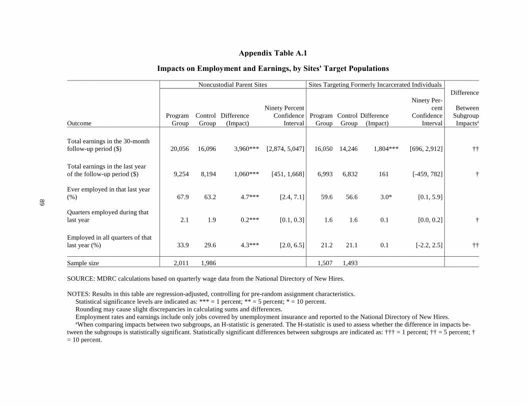
Appendix Table A.1
Impacts on Employment and Earnings, by Sites' Target Populations
Noncustodial Parent Sites Sites Targeting Formerly Incarcerated Individuals Difference
Ninety Percent Ninety Per-
cent Between Program Control Difference Confidence Program Control Difference Confidence Subgroup
Outcome Group Group (Impact) Interval Group Group (Impact) Interval Impactsa Total earnings in the 30-month follow-up period ($) 20,056 16,096 3,960 *** [2,874, 5,047] 16,050 14,246 1,804 *** [696, 2,912] †† Total earnings in the last year of the follow-up period ($) 9,254 8,194 1,060 *** [451, 1,668] 6,993 6,832 161 [-459, 782] † Ever employed in that last year (%) 67.9 63.2 4.7 *** [2.4, 7.1] 59.6 56.6 3.0 * [0.1, 5.9] Quarters employed during that last year 2.1 1.9 0.2 *** [0.1, 0.3] 1.6 1.6 0.1 [0.0, 0.2] † Employed in all quarters of that last year (%) 33.9 29.6 4.3 *** [2.0, 6.5] 21.2 21.1 0.1 [-2.2, 2.5] †† Sample size 2,011 1,986 1,507 1,493 SOURCE: MDRC calculations based on quarterly wage data from the National Directory of New Hires. NOTES: Results in this table are regression-adjusted, controlling for pre-random assignment characteristics. Statistical significance levels are indicated as: *** = 1 percent; ** = 5 percent; * = 10 percent. Rounding may cause slight discrepancies in calculating sums and differences. Employment rates and earnings include only jobs covered by unemployment insurance and reported to the National Directory of New Hires. aWhen comparing impacts between two subgroups, an H-statistic is generated. The H-statistic is used to assess whether the difference in impacts be-tween the subgroups is statistically significant. Statistically significant differences between subgroups are indicated as: ††† = 1 percent; †† = 5 percent; † = 10 percent.
89
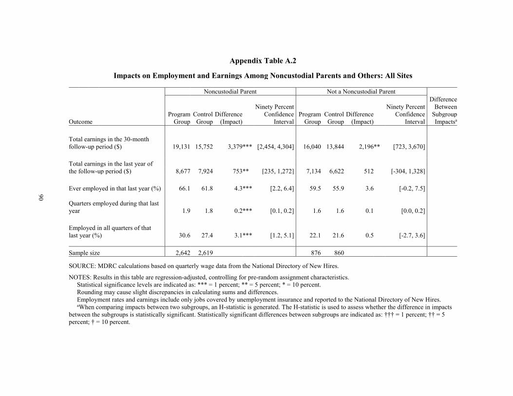
Appendix Table A.2
t
h
f
t
t
Impacts on Employment and Earnings Among Noncustodial Parents and Others: All Sites
Noncustodial Parent Not a Noncustodial Parent Difference
Ninety Percen Ninety Percent Between Program Control Difference Confidence Program Control Difference Confidence Subgroup
Outcome Group Group (Impact) Interval Group Group (Impact) Interval Impactsa
Total earnings in the 30-montfollow-up period ($) 19,131 15,752 3,379 *** [2,454, 4,304] 16,040 13,844 2,196 ** [723, 3,670]
Total earnings in the last year othe follow-up period ($) 8,677 7,924 753 ** [235, 1,272] 7,134 6,622 512 [-304, 1,328]
Ever employed in that last year (%) 66.1 61.8 4.3 *** [2.2, 6.4] 59.5 55.9 3.6 [-0.2, 7.5]
Quarters employed during that lasyear 1.9 1.8 0.2 *** [0.1, 0.2] 1.6 1.6 0.1 [0.0, 0.2]
Employed in all quarters of thalast year (%) 30.6 27.4 3.1 *** [1.2, 5.1] 22.1 21.6 0.5 [-2.7, 3.6]
Sample size 2,642 2,619 876 860
SOURCE: MDRC calculations based on quarterly wage data from the National Directory of New Hires.
NOTES: Results in this table are regression-adjusted, controlling for pre-random assignment characteristics. Statistical significance levels are indicated as: *** = 1 percent; ** = 5 percent; * = 10 percent. Rounding may cause slight discrepancies in calculating sums and differences. Employment rates and earnings include only jobs covered by unemployment insurance and reported to the National Directory of New Hires. aWhen comparing impacts between two subgroups, an H-statistic is generated. The H-statistic is used to assess whether the difference in impacts between the subgroups is statistically significant. Statistically significant differences between subgroups are indicated as: ††† = 1 percent; †† = 5 percent; † = 10 percent.
90
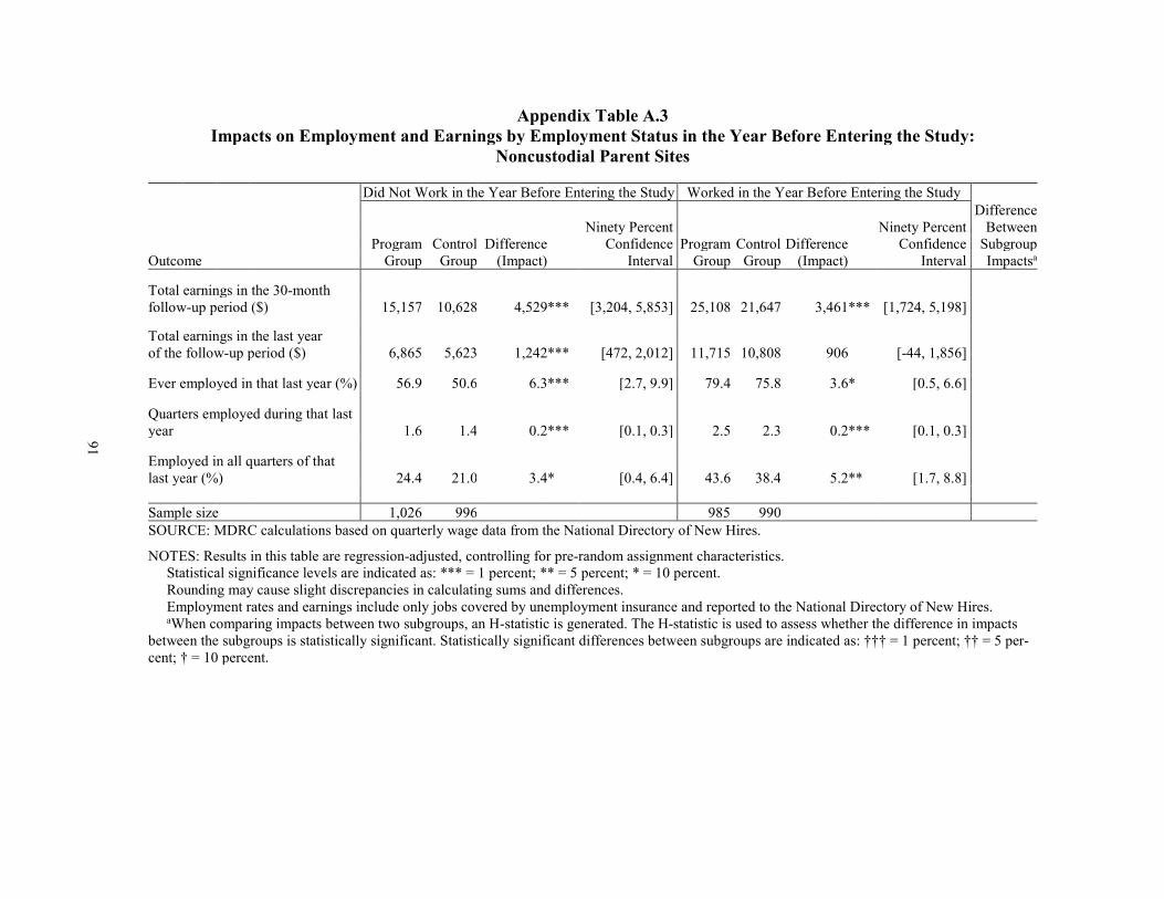
Appendix Table A.3 Impacts on Employment and Earnings by Employment Status in the Year Before Entering the Study:
Noncustodial Parent Sites
Did Not Work in the Year Before Entering the Study Worked in the Year Before Entering the Study
t
Difference Ninety Percen Ninety Percent Between
Program Control Difference Confidence Program Control Difference Confidence Subgroup Outcome Group Group (Impact) Interval Group Group (Impact) Interval Impactsa
Total earnings in the 30-monthfollow-up period ($) 15,157 10,628 4,529 *** [3,204, 5,853] 25,108 21,647 3,461 *** [1,724, 5,198]
Total earnings in the last yearof the follow-up period ($) 6,865 5,623 1,242 *** [472, 2,012] 11,715 10,808 906 [-44, 1,856]
Ever employed in that last year (%) 56.9 50.6 6.3 *** [2.7, 9.9] 79.4 75.8 3.6 * [0.5, 6.6]
Quarters employed during that last year 1.6 1.4 0.2 *** [0.1, 0.3] 2.5 2.3 0.2 *** [0.1, 0.3]
Employed in all quarters of that last year (%) 24.4 21.0 3.4 * [0.4, 6.4] 43.6 38.4 5.2 ** [1.7, 8.8]
Sample size 1,026 996 985 990 SOURCE: MDRC calculations based on quarterly wage data from the National Directory of New Hires.
NOTES: Results in this table are regression-adjusted, controlling for pre-random assignment characteristics. Statistical significance levels are indicated as: *** = 1 percent; ** = 5 percent; * = 10 percent. Rounding may cause slight discrepancies in calculating sums and differences. Employment rates and earnings include only jobs covered by unemployment insurance and reported to the National Directory of New Hires. aWhen comparing impacts between two subgroups, an H-statistic is generated. The H-statistic is used to assess whether the difference in impacts between the subgroups is statistically significant. Statistically significant differences between subgroups are indicated as: ††† = 1 percent; †† = 5 per-cent; † = 10 percent.
91

(continued)
Appendix Table A.4
Impacts on Employment and Earnings, Child Support, and Criminal Justice Outcomes, by Level of Education
Does Not Have a High School Diploma Has a High School Diploma
Ninety Percent Confidence
Interval
Ninety Percent Confidence Interval
Difference Between
Subgroup Impactsa
Program Group
Control Difference (Impact) Group
Program Group
Control Group
Difference (Impact) Outcome
Employment and earnings: all sites Total earnings in the 30-month follow-up period ($) 15,147 10,789 4,359 *** [3,139, 5,578] 19,695 17,028 2,667 *** [1,636, 3,698] †
Total earnings in the last year of the follow-up period ($) 6,697 5,423 1,274 *** [581, 1,966] 9,034 8,452 582 * [7, 1,157]
Ever employed in that last year (%) 61.1 53.6 7.5 *** [3.8, 11.3] 65.9 63.4 2.5 * [0.3, 4.7] †
Quarters employed during that last year 1.7 1.5 0.2 *** [0.1, 0.3] 1.9 1.8 0.1 ** [0.0, 0.2]
Employed in all quarters of that last year (%) 24.9 21.8 3.1 [-0.1, 6.2] 30.0 28.1 1.9 [-0.2, 4.0]
Sample size 875 880 2,392 2,238
Child support: noncustodial parent sites Total child support paid in the 30-month follow-up period ($) 2,240 2,113 127 [-518, 772] 3,127 2,929 198 [-121, 518]
Amount of formal child support paid in the last year of the follow-up period ($) 1,015 1,032 -17 [-356, 322] 1,315 1,402 -88 [-260, 85]
Paid any formal child support in that last year (%) 55.8 46.9 8.9 *** [4.1, 13.7] 64.4 59.1 5.3 *** [2.3, 8.3]
Sample size 507 519 1,317 1,180
92
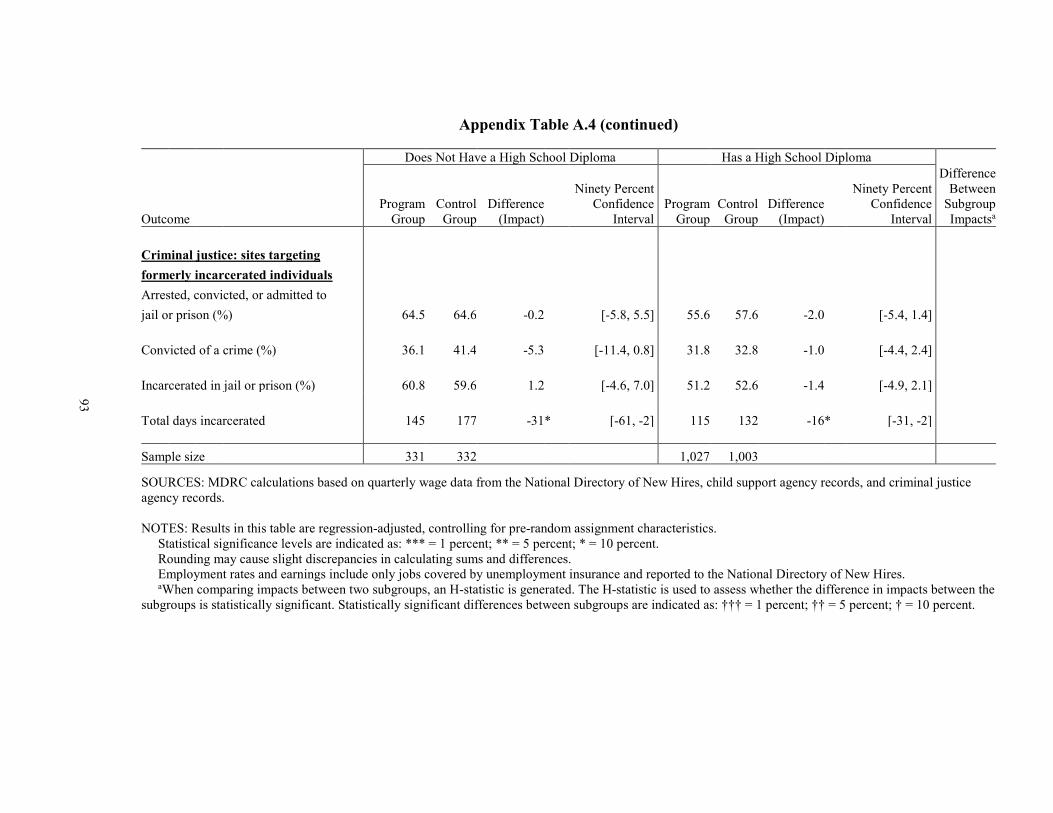
Appendix Table A.4 (continued)
Does Not Have a High School Diploma Has a High School Diploma
Ninety Percent Ninety Percent Difference
Between Program Control Difference Confidence Program Control Difference Confidence Subgroup
Outcome Group Group (Impact) Interval Group Group (Impact) Interval Impactsa Criminal justice: sites targeting formerly incarcerated individuals Arrested, convicted, or admitted to jail or prison (%) 64.5 64.6 -0.2 [-5.8, 5.5] 55.6 57.6 -2.0 [-5.4, 1.4]
Convicted of a crime (%) 36.1 41.4 -5.3 [-11.4, 0.8] 31.8 32.8 -1.0 [-4.4, 2.4]
Incarcerated in jail or prison (%) 60.8 59.6 1.2 [-4.6, 7.0] 51.2 52.6 -1.4 [-4.9, 2.1]
Total days incarcerated 145 177 -31 * [-61, -2] 115 132 -16 * [-31, -2]
Sample size 331 332 1,027 1,003
SOURCES: MDRC calculations based on quarterly wage data from the National Directory of New Hires, child support agency records, and criminal justice agency records. NOTES: Results in this table are regression-adjusted, controlling for pre-random assignment characteristics. Statistical significance levels are indicated as: *** = 1 percent; ** = 5 percent; * = 10 percent. Rounding may cause slight discrepancies in calculating sums and differences. Employment rates and earnings include only jobs covered by unemployment insurance and reported to the National Directory of New Hires. aWhen comparing impacts between two subgroups, an H-statistic is generated. The H-statistic is used to assess whether the difference in impacts between the subgroups is statistically significant. Statistically significant differences between subgroups are indicated as: ††† = 1 percent; †† = 5 percent; † = 10 percent.
93
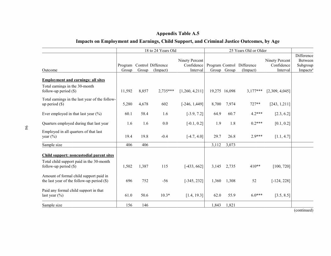
(continued)
t
h
Appendix Table A.5 Impacts on Employment and Earnings, Child Support, and Criminal Justice Outcomes, by Age
18 to 24 Years Old 25 Years Old or Older
Ninety Percen Ninety Percent Difference
Between Program Control Difference Confidence Program Control Difference Confidence Subgroup
Outcome Group Group (Impact) Interval Group Group (Impact) Interval Impactsa
Employment and earnings: all sites Total earnings in the 30-montfollow-up period ($) 11,592 8,857 2,735 *** [1,260, 4,211] 19,275 16,098 3,177 *** [2,309, 4,045]
Total earnings in the last year of the follow-up period ($) 5,280 4,678 602 [-246, 1,449] 8,700 7,974 727 ** [243, 1,211]
Ever employed in that last year (%) 60.1 58.4 1.6 [-3.9, 7.2] 64.9 60.7 4.2 *** [2.3, 6.2]
Quarters employed during that last year 1.6 1.6 0.0 [-0.1, 0.2] 1.9 1.8 0.2 *** [0.1, 0.2]
Employed in all quarters of that last year (%) 19.4 19.8 -0.4 [-4.7, 4.0] 29.7 26.8 2.9 *** [1.1, 4.7]
Sample size 406 406 3,112 3,073
Child support: noncustodial parent sites Total child support paid in the 30-month follow-up period ($) 1,502 1,387 115 [-433, 662] 3,145 2,735 410 ** [100, 720]
Amount of formal child support paid in the last year of the follow-up period ($) 696 752 -56 [-345, 232] 1,360 1,308 52 [-124, 228]
Paid any formal child support in that last year (%) 61.0 50.6 10.3 * [1.4, 19.3] 62.0 55.9 6.0 *** [3.5, 8.5]
Sample size 156 146 1,843 1,821
94
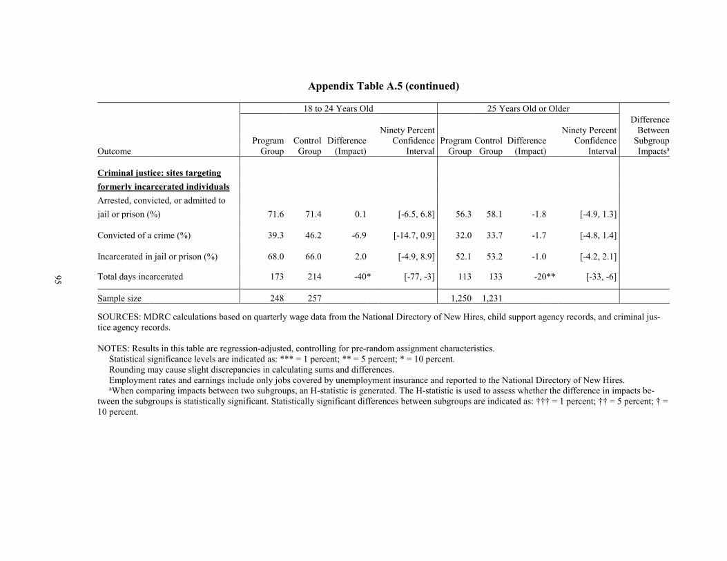
Appendix Table A.5 (continued)
18 to 24 Years Old 25 Years Old or Older
Ninety Percent Ninety Percent Difference
Between Program Control Difference Confidence Program Control Difference Confidence Subgroup
Outcome Group Group (Impact) Interval Group Group (Impact) Interval Impactsa
Criminal justice: sites targeting formerly incarcerated individuals Arrested, convicted, or admitted to jail or prison (%) 71.6 71.4 0.1 [-6.5, 6.8] 56.3 58.1 -1.8 [-4.9, 1.3]
Convicted of a crime (%) 39.3 46.2 -6.9 [-14.7, 0.9] 32.0 33.7 -1.7 [-4.8, 1.4]
Incarcerated in jail or prison (%) 68.0 66.0 2.0 [-4.9, 8.9] 52.1 53.2 -1.0 [-4.2, 2.1]
Total days incarcerated 173 214 -40 * [-77, -3] 113 133 -20 ** [-33, -6]
Sample size 248 257 1,250 1,231
SOURCES: MDRC calculations based on quarterly wage data from the National Directory of New Hires, child support agency records, and criminal jus-tice agency records. NOTES: Results in this table are regression-adjusted, controlling for pre-random assignment characteristics. Statistical significance levels are indicated as: *** = 1 percent; ** = 5 percent; * = 10 percent. Rounding may cause slight discrepancies in calculating sums and differences. Employment rates and earnings include only jobs covered by unemployment insurance and reported to the National Directory of New Hires. aWhen comparing impacts between two subgroups, an H-statistic is generated. The H-statistic is used to assess whether the difference in impacts be-tween the subgroups is statistically significant. Statistically significant differences between subgroups are indicated as: ††† = 1 percent; †† = 5 percent; † = 10 percent.
94 95
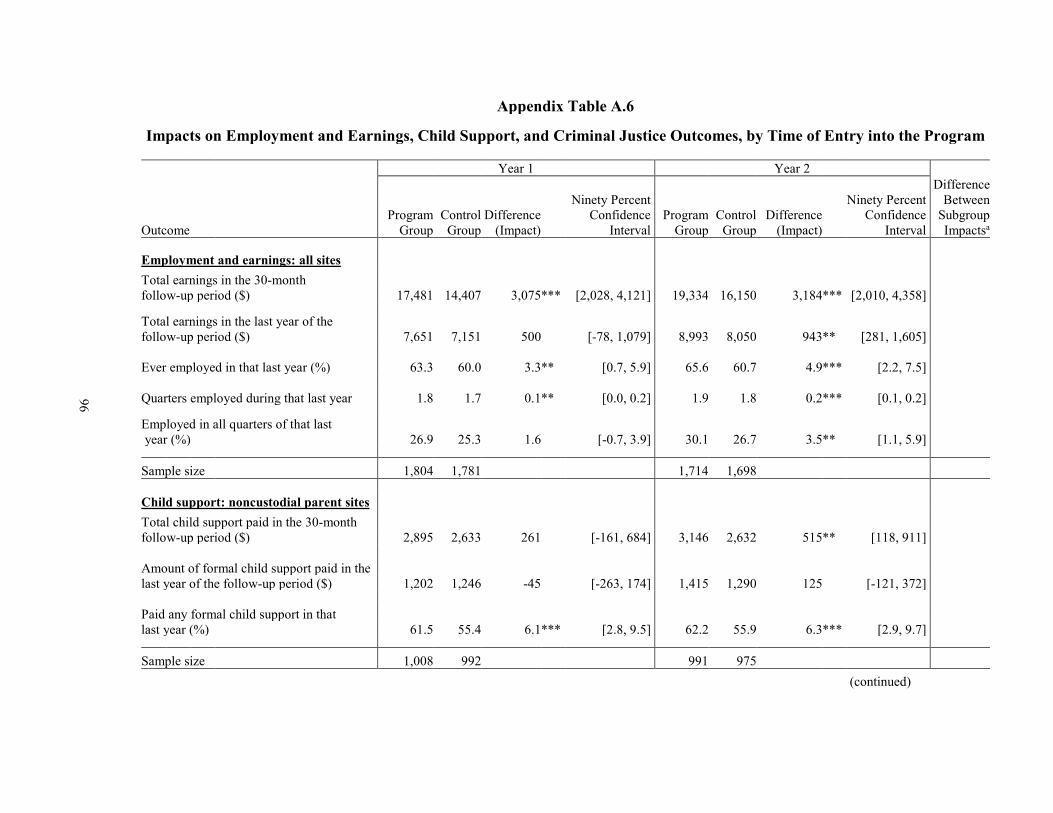
(continued)
Appendix Table A.6
Impacts on Employment and Earnings, Child Support, and Criminal Justice Outcomes, by Time of Entry into the Program
Year 1 Year 2
Ninety Percent Ninety Percent Difference
Between Program Control Difference Confidence Program Control Difference Confidence Subgroup
Outcome Group Group (Impact) Interval Group Group (Impact) Interval Impactsa
Employment and earnings: all sites Total earnings in the 30-month follow-up period ($) 17,481 14,407 3,075 *** [2,028, 4,121] 19,334 16,150 3,184 *** [2,010, 4,358]
Total earnings in the last year of the follow-up period ($) 7,651 7,151 500 [-78, 1,079] 8,993 8,050 943 ** [281, 1,605]
Ever employed in that last year (%) 63.3 60.0 3.3 ** [0.7, 5.9] 65.6 60.7 4.9 *** [2.2, 7.5]
Quarters employed during that last year 1.8 1.7 0.1 ** [0.0, 0.2] 1.9 1.8 0.2 *** [0.1, 0.2]
Employed in all quarters of that last year (%) 26.9 25.3 1.6 [-0.7, 3.9] 30.1 26.7 3.5 ** [1.1, 5.9]
Sample size 1,804 1,781 1,714 1,698
Child support: noncustodial parent sites Total child support paid in the 30-month follow-up period ($) 2,895 2,633 261 [-161, 684] 3,146 2,632 515 ** [118, 911]
Amount of formal child support paid in the last year of the follow-up period ($) 1,202 1,246 -45 [-263, 174] 1,415 1,290 125 [-121, 372]
Paid any formal child support in that last year (%) 61.5 55.4 6.1 *** [2.8, 9.5] 62.2 55.9 6.3 *** [2.9, 9.7]
Sample size 1,008 992 991 975
96
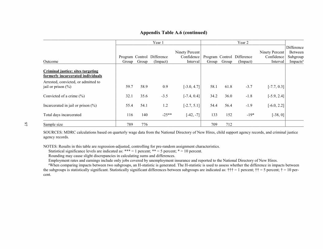
Appendix Table A.6 (continued)
Year 1 Year 2
Ninety Percent Ninety Percent Difference
Between Program Control Difference Confidence Program Control Difference Confidence Subgroup
Outcome Group Group (Impact) Interval Group Group (Impact) Interval Impactsa
Criminal justice: sites targeting formerly incarcerated individuals Arrested, convicted, or admitted to jail or prison (%) 59.7 58.9 0.9 [-3.0, 4.7] 58.1 61.8 -3.7 [-7.7, 0.3]
Convicted of a crime (%) 32.1 35.6 -3.5 [-7.4, 0.4] 34.2 36.0 -1.8 [-5.9, 2.4]
Incarcerated in jail or prison (%) 55.4 54.1 1.2 [-2.7, 5.1] 54.4 56.4 -1.9 [-6.0, 2.2]
Total days incarcerated 116 140 -25 ** [-42, -7] 133 152 -19 * [-38, 0]
Sample size 789 776 709 712
SOURCES: MDRC calculations based on quarterly wage data from the National Directory of New Hires, child support agency records, and criminal justice agency records. NOTES: Results in this table are regression-adjusted, controlling for pre-random assignment characteristics. Statistical significance levels are indicated as: *** = 1 percent; ** = 5 percent; * = 10 percent. Rounding may cause slight discrepancies in calculating sums and differences. Employment rates and earnings include only jobs covered by unemployment insurance and reported to the National Directory of New Hires. aWhen comparing impacts between two subgroups, an H-statistic is generated. The H-statistic is used to assess whether the difference in impacts between the subgroups is statistically significant. Statistically significant differences between subgroups are indicated as: ††† = 1 percent; †† = 5 percent; † = 10 per-cent.
97

THIS PAGE INTENTIONALLY LEFT BLANK

Appendix B
Supplementary Tables and Figures for Atlanta

THIS PAGE INTENTIONALLY LEFT BLANK
101
Appendix Table B.1
(continued)
Impacts on Employment and Earnings: Atlanta
Program Control Difference Ninety Percent Outcome Group Group (Impact) Confidence Interval
Outcomes based on administrative dataa Total earnings during the 30-month follow-up period ($) 30,329 25,588 4,741 *** [2,000, 7,482]
Total earnings in the last year of the follow-up period ($) 14,098 13,168 930 [-595, 2,456]
Ever employed in that last year (%) 79.1 74.1 5.0 * [0.8, 9.3]
Quarters employed during that last year 2.6 2.4 0.2 ** [0.0, 0.4]
Employed in all quarters of that last year (%) 48.9 45.0 3.9 [-1.2, 9.0]
Sample size 501 495
Self-reported outcomes based on survey data Ever employed in the last year of the follow-up period (%) 91.7 84.4 7.3 *** [3.6, 11.0]
Employed at the time of the 30-month survey (%) 76.0 71.8 4.1 [-0.9, 9.1] Employed and earning more than $10 per hour 43.7 34.8 8.9 ** [3.0, 14.8]
Hours worked per week at the time of the 30-month survey (%)
More than 20 hours 71.4 64.3 7.1 ** [1.8, 12.5] More than 34 hours 59.3 53.0 6.3 * [0.6, 12.1]
Type of employment at the time of the 30-month survey (%) Not currently employed 26.7 31.6 -4.9 [-10.3, 0.6] Permanent 61.9 53.8 8.1 ** [2.1, 14.1] Temporary, including day labor and odd jobs 10.5 14.1 -3.6 [-7.7, 0.5] Other 0.9 0.5 0.4 [-0.7, 1.4]
Among those currently employed at the time of the 30-month survey:b
Hours worked per week 40.2 40.3 -0.1 Hourly wage ($) 12.3 11.8 0.5
Sample size 409 393

102
Appendix Table B.1 (continued) SOURCES: MDRC calculations based on quarterly wage data from the National Directory of New Hires and responses to the ETJD 30-month survey. NOTES: Results in this table are regression-adjusted, controlling for pre-random assignment characteris-tics. Analyses of survey-based outcomes incorporate weights that correct for survey nonresponse, which take into consideration information on the full sample’s pre-random assignment characteristics. Un-weighted analyses (not shown) yielded nearly identical results. Statistical significance levels are indicated as: *** = 1 percent; ** = 5 percent; * = 10 percent. Rounding may cause slight discrepancies in calculating sums and differences. aEmployment rates and earnings include only jobs covered by unemployment insurance and reported to the National Directory of New Hires. bThese measures are calculated among those employed at the time of the survey; they are therefore considered nonexperimental and are not tested for statistical significance.
103
Appendix Table B.2
(continued)
Impacts on Child Support and Family Relationships: Atlanta
Ninety Percent Program Control Difference Confidence Outcome Group Group (Impact) Interval
Outcomes based on administrative data Amount of formal child support paid in the last year of the follow-up period ($) 1,987 1,652 335 ** [94, 577]
Paid any formal child support in that last yeara (%) 72.9 70.6 2.3 [-2.4, 7.0]
Months of formal child support paid in that last year 6.0 5.4 0.5 * [0.0, 1.0]
Among those who paid formal child support: Months from random assignment to first paymentb 2.6 5.7 -3.1
Sample size 501 495
Self-reported outcomes based on survey data (%) Currently a noncustodial parent of a minor-age child 64.2 59.5 4.7 [-0.6, 10.0]
Provided informal cash support or noncash support in the past month 48.8 47.4 1.3 [-4.3, 7.0]
Informal cash support 37.4 33.5 3.9 [-1.5, 9.3] Noncash support 43.9 42.9 1.1 [-4.5, 6.6]
Owing child support affects willingness to take jobs 27.6 22.2 5.5 [-0.4, 11.3]
Incarcerated for not paying child support 6.0 7.7 -1.7 [-4.7, 1.2]
Frequency of contact with the focal child in the past 3 monthsc
A few times a week or more 32.4 35.1 -2.7 [-8.2, 2.9] A few times a month 12.2 14.4 -2.3 [-6.4, 1.9] Less than a few times a month 4.9 8.4 -3.5 * [-6.5, -0.5] Not at all 23.1 15.7 7.4 ** [2.7, 12.1] No minor-aged children 27.4 26.4 1.0 [-3.8, 5.8]
Sample size 409 392

104
Appendix Table B.2 (continued) SOURCES: MDRC calculations based on child support agency data and responses to the ETJD 30-month survey. NOTES: Results in this table are regression-adjusted, controlling for pre-random assignment characteris-tics. Analyses of survey-based outcomes incorporate weights that correct for survey nonresponse, which take into consideration information on the full sample’s pre-random assignment characteristics. Un-weighted analyses (not shown) yielded nearly identical results. Statistical significance levels are indicated as: *** = 1 percent; ** = 5 percent; * = 10 percent. Rounding may cause slight discrepancies in calculating sums and differences. aMeasures of formal child support include all payments made through the state’s child support collec-tion and disbursement unit, including funds from employer withholding and other sources (for example, intercepted tax refunds). bThis measure is calculated among those who paid child support during the follow-up period; it is therefore considered nonexperimental and is not tested for statistical significance. cThe focal child is defined as the youngest minor-age child living outside of the sample member's household; if the sample member reports no minor-age children living outside of his or her household, the focal child is the youngest minor-age child residing within the household. A contact is defined as spend-ing one or more hours a day with the focal child.
105
Appendix Table B.3
Impacts on Criminal Justice Outcomes: Atlanta
Ninety Percent Program Control Difference Confidence Outcome Group Group (Impact) Interval
Self-reported outcomes based on survey dataa Incarcerated (%) 13.7 16.3 -2.5 [-6.7, 1.6]
Incarcerated for not paying child support (%) 6.0 7.7 -1.7 [-4.7, 1.2]
Total days incarcerated 14.0 10.4 3.6 [-3.4, 10.5]
On parole or probation since entering the study (%) 26.3 23.2 3.1 [-1.7, 8.0]
Received a technical violation of parole or probation (%) 3.2 2.0 1.2 [-0.7, 3.1]
Received a sanction for a technical parole violation (%) 2.3 1.7 0.5 [-1.1, 2.2]
Sample size 409 392
SOURCE: MDRC calculations based on responses to the ETJD 30-month survey.
NOTES: Results in this table are regression-adjusted, controlling for pre-random assignment characteris-tics. Analyses of survey-based outcomes incorporate weights that correct for survey nonresponse, which take into consideration information on the full sample’s pre-random assignment characteristics. Un-weighted analyses (not shown) yielded nearly identical results. Statistical significance levels are indicated as: *** = 1 percent; ** = 5 percent; * = 10 percent. Rounding may cause slight discrepancies in calculating sums and differences. aMeasures include occurrences at any point between random assignment and the time of the 30-month survey.
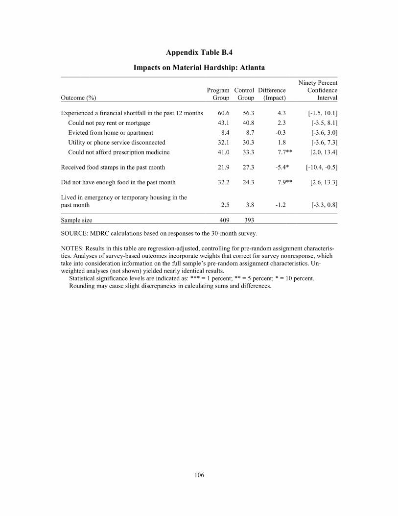
106
Appendix Table B.4
Impacts on Material Hardship: Atlanta
Ninety Percent Program Control Difference Confidence Outcome (%) Group Group (Impact) Interval
Experienced a financial shortfall in the past 12 months 60.6 56.3 4.3 [-1.5, 10.1] Could not pay rent or mortgage 43.1 40.8 2.3 [-3.5, 8.1] Evicted from home or apartment 8.4 8.7 -0.3 [-3.6, 3.0] Utility or phone service disconnected 32.1 30.3 1.8 [-3.6, 7.3] Could not afford prescription medicine 41.0 33.3 7.7 ** [2.0, 13.4]
Received food stamps in the past month 21.9 27.3 -5.4 * [-10.4, -0.5]
Did not have enough food in the past month 32.2 24.3 7.9 ** [2.6, 13.3]
Lived in emergency or temporary housing in the past month 2.5 3.8 -1.2 [-3.3, 0.8]
Sample size 409 393
SOURCE: MDRC calculations based on responses to the 30-month survey.
NOTES: Results in this table are regression-adjusted, controlling for pre-random assignment characteris-tics. Analyses of survey-based outcomes incorporate weights that correct for survey nonresponse, which take into consideration information on the full sample’s pre-random assignment characteristics. Un-weighted analyses (not shown) yielded nearly identical results. Statistical significance levels are indicated as: *** = 1 percent; ** = 5 percent; * = 10 percent. Rounding may cause slight discrepancies in calculating sums and differences.
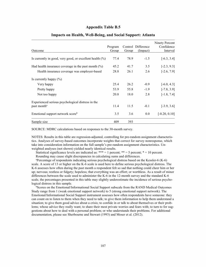
107
Appendix Table B.5
Experienced serious psychological distress in the
b
Impacts on Health, Well-Being, and Social Support: Atlanta
Ninety Percent Program Control Difference Confidence Outcome Group Group (Impact) Interval
Is currently in good, very good, or excellent health (%) 77.4 78.9 -1.5 [-6.3, 3.4]
Had health insurance coverage in the past month (%) 45.2 41.7 3.5 [-2.3, 9.3] Health insurance coverage was employer-based 28.8 26.1 2.6 [-2.6, 7.9]
Is currently happy (%) Very happy 25.4 26.2 -0.9 [-6.0, 4.3] Pretty happy 53.9 55.8 -1.9 [-7.8, 3.9] Not too happy 20.8 18.0 2.8 [-1.8, 7.4]
past montha 11.4 11.5 -0.1 [-3.9, 3.6]
Emotional support network score 3.5 3.6 0.0 [-0.20, 0.10]
Sample size 409 393
SOURCE: MDRC calculations based on responses to the 30-month survey.
NOTES: Results in this table are regression-adjusted, controlling for pre-random assignment characteris-tics. Analyses of survey-based outcomes incorporate weights that correct for survey nonresponse, which take into consideration information on the full sample’s pre-random assignment characteristics. Un-weighted analyses (not shown) yielded nearly identical results. Statistical significance levels are indicated as: *** = 1 percent; ** = 5 percent; * = 10 percent. Rounding may cause slight discrepancies in calculating sums and differences. aPercentage of respondents indicating serious psychological distress based on the Kessler-6 (K-6) scale. A score of 13 or higher on the K-6 scale is used here to define serious psychological distress. The K-6 assesses how often during the past month a respondent felt so sad that nothing could cheer him or her up; nervous; restless or fidgety; hopeless; that everything was an effort; or worthless. As a result of minor differences between the scale used to administer the K-6 in the 12-month survey and the standard K-6 scale, the percentages presented in this table may slightly underestimate the incidence of serious psycho-logical distress in this sample. bScores on the Emotional/Informational Social Support subscale from the RAND Medical Outcomes Study range from 1 (weak emotional support network) to 5 (strong emotional support network). The Emotional/Informational Social Support instrument assesses how often respondents have someone: they can count on to listen to them when they need to talk; to give them information to help them understand a situation; to give them good advice about a crisis; to confide in or talk to about themselves or their prob-lems; whose advice they really want; to share their most private worries and fears with; to turn to for sug-gestions about how to deal with a personal problem; or who understands their problems. For additional documentation, please see Sherbourne and Stewart (1993) and Moser et al. (2012).
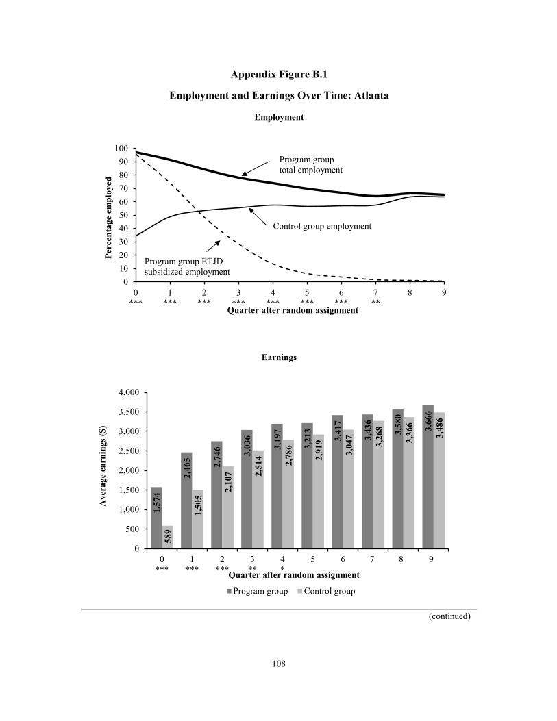
108
(continued)
Appendix Figure B.1
Employment and Earnings Over Time: Atlanta
Employment
Earnings
0102030405060708090
100
0***
1***
2***
3***
4***
5***
6***
7**
8 9
Perc
enta
ge e
mpl
oyed
Quarter after random assignment
Program group total employment
Control group employment
1,57
4
2,46
5 2,74
6 3,03
6
3,19
7
3,21
3
3,41
7
3,43
6
3,58
0
3,66
6
589
1,50
5
2,10
7 2,51
4 2,78
6
2,91
9
3,04
7
3,26
8
3,36
6
3,48
6
0
500
1,000
1,500
2,000
2,500
3,000
3,500
4,000
0***
1***
2***
3**
4*
5 6 7 8 9
Ave
rage
ear
ning
s ($)
Quarter after random assignment
Program group Control group
Program group ETJDsubsidized employment

109
Appendix Figure B.1 (continued)
SOURCES: MDRC calculations based on quarterly wage data from the National Directory of New Hiresand program payroll records.
NOTES: Results in this figure are regression-adjusted, controlling for pre-random assignment characteristics.
Statistical significance levels are indicated as: *** = 1 percent; ** = 5 percent; * = 10 percent.Employment rates and earnings in the quarter of random assignment through Quarter 5 after random
assignment include both ETJD subsidized jobs and jobs covered by unemployment insurance and reported to the National Directory of New Hires. Employment rates and earnings in Quarters 6 through 9 after random assignment include only jobs covered by unemployment insurance and reported to the National Directory of New Hires.
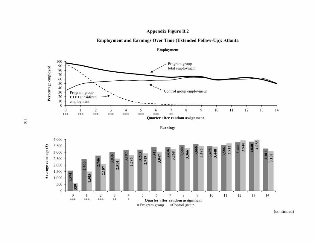
(continued)
Appendix Figure B.2
Employment and Earnings Over Time (Extended Follow-Up): Atlanta
Employment
Earnings
0102030405060708090
100
0***
1***
2***
3***
4***
5***
6***
7**
8 9 10 11 12 13 14
Perc
enta
ge e
mpl
oyed
Quarter after random assignment
Program group total employment
Control group employment
1,57
4
2,46
5
2,74
6
3,03
6
3,19
7
3,21
3
3,41
7
3,43
6
3,58
0
3,66
6
3,49
8
3,58
6
3,78
6
3,84
0
3,30
1
589
1,50
5 2,10
7 2,51
4
2,78
6
2,91
9
3,04
7
3,26
8
3,36
6
3,48
6
3,44
8
3,71
2
3,94
0
3,10
2
0500
1,0001,5002,0002,5003,0003,5004,000
0***
1***
2***
3**
4*
5 6 7 8 9 10 11 12 13 14
Ave
rage
ear
ning
s ($)
Quarter after random assignmentProgram group Control Group
4,05
8
Control group
Program group ETJD subsidized employment
110

111
Appendix Figure B.2 (continued) SOURCES: MDRC calculations based on quarterly wage data from the National Directory of New Hires and program payroll records. NOTES: Results in this figure are regression-adjusted, controlling for pre-random assignment character-istics. Statistical significance levels are indicated as: *** = 1 percent; ** = 5 percent; * = 10 percent. Employment rates and earnings in the quarter of random assignment through Quarter 5 after random assignment include both ETJD subsidized jobs and jobs covered by unemployment insurance and re-ported to the National Directory of New Hires. Employment rates and earnings in Quarters 6 through 14 after random assignment include only jobs covered by unemployment insurance and reported to the Na-tional Directory of New Hires.
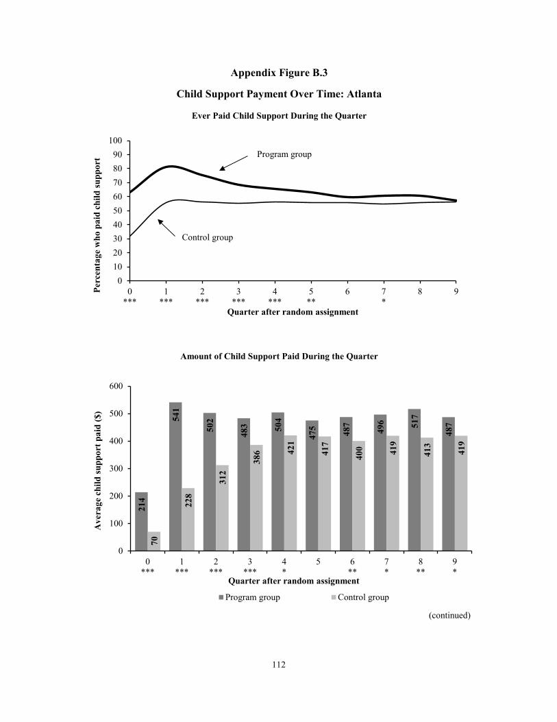
112
(continued)
Appendix Figure B.3
Child Support Payment Over Time: Atlanta Ever Paid Child Support During the Quarter
Amount of Child Support Paid During the Quarter
0102030405060708090
100
0***
1***
2***
3***
4***
5**
6 7*
8 9Perc
enta
ge w
ho p
aid
child
supp
ort
Quarter after random assignment
Program group
Control group
214
541
502
483 50
4
475 487
496 51
7
487
70
228
312
386 42
1
417
400 41
9
413
419
0
100
200
300
400
500
600
0***
1***
2***
3***
4*
5 6**
7*
8**
9*
Ave
rage
chi
ld su
ppor
t pai
d ($
)
Quarter after random assignment
Program group Control group

113
Appendix Figure B.3 (continued)
SOURCE: MDRC calculations based on child support agency data.
NOTES: Results in this figure are regression-adjusted, controlling for pre-random assignment characteristics.
Statistical significance levels are indicated as: *** = 1 percent; ** = 5 percent; * = 10 percent.

THIS PAGE INTENTIONALLY LEFT BLANK

Appendix C
Supplementary Tables and Figures for Milwaukee

THIS PAGE INTENTIONALLY LEFT BLANK

117
Appendix Table C.1
(continued)
Impacts on Employment and Earnings: Milwaukee
Outcome Program
Group Control
Group Difference
(Impact)
Ninety Percent Confidence
Interval
Outcomes based on administrative dataa Total earnings during the 30 months of follow-up ($) 15,159 12,284 2,875 *** [1,292, 4,459]
Total earnings in the last year of the follow-up period ($) 7,160 6,592 567 [-364, 1,499]
Ever employed in that last year (%) 71.6 69.2 2.5 [-2.1, 7.1]
Quarters employed during that last year 2.1 1.9 0.2 * [0.0, 0.3]
Employed in all quarters of that last year (%) 31.5 27.7 3.8 [-0.8, 8.4]
Sample size 502 501
Self-reported outcomes based on survey data Ever employed in the last year of the follow-up period (%) 80.8 79.6 1.2 [-3.4, 5.9]
Employed at the time of the 30-month survey (%) 52.4 52.8 -0.5 [-6.3, 5.4] Employed and earning more than $10 per hour 20.7 18.9 1.8 [-2.9, 6.6]
Hours worked per week at the time of the 30-month survey (%)
More than 20 hours 43.0 40.5 2.5 [-3.3, 8.3] More than 34 hours 33.5 31.5 2.0 [-3.6, 7.6]
Type of employment at the time of the 30-month survey (%)
Not currently employed 51.8 51.3 0.6 [-5.6, 6.7] Permanent 32.6 33.8 -1.2 [-6.9, 4.6] Temporary, including day labor and odd jobs 15.3 15.0 0.3 [-4.1, 4.8] Other 0.3 0.0 0.3 [-0.2, 0.7]
Among those currently employed at the time of the 30-month survey:b
Hours worked per week 35.2 34.8 0.4 Hourly wage ($) 11.2 10.5 0.7
Sample size 401 382

118
Appendix Table C.1 (continued) SOURCES: MDRC calculations based on quarterly wage data from the National Directory of New Hires and responses to the ETJD 30-month survey. NOTES: Results in this table are regression-adjusted, controlling for pre-random assignment characteris-tics. Analyses of survey-based outcomes incorporate weights that correct for survey nonresponse, which take into consideration information on the full sample’s pre-random assignment characteristics. Un-weighted analyses (not shown) yielded nearly identical results. Statistical significance levels are indicated as: *** = 1 percent; ** = 5 percent; * = 10 percent. aEmployment rates and earnings include only jobs covered by unemployment insurance and reported to the National Directory of New Hires. bThese measures are calculated among those employed at the time of the survey; they are therefore considered nonexperimental and are not tested for statistical significance.
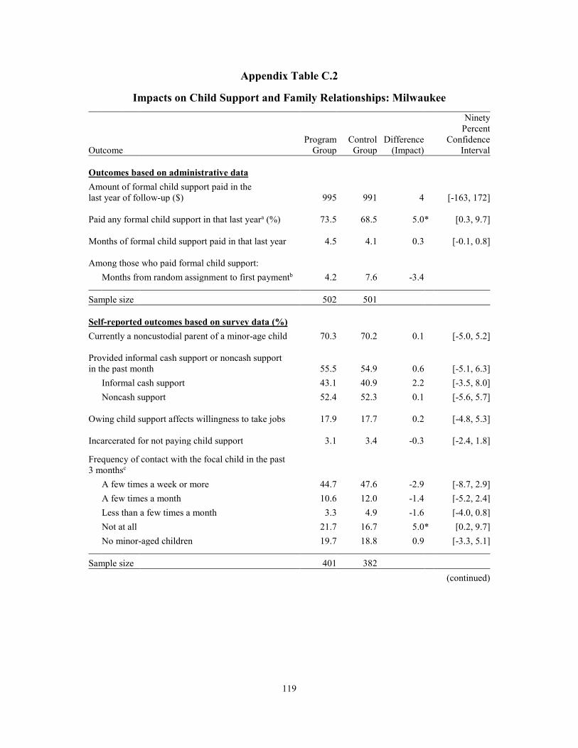
119
Appendix Table C.2
(continued)
Impacts on Child Support and Family Relationships: Milwaukee
Outcome
Program
Group
Control
Group
Difference
(Impact)
Ninety Percent
Confidence Interval
Outcomes based on administrative data Amount of formal child support paid in the last year of follow-up ($) 995 991 4 [-163, 172]
Paid any formal child support in that last yeara (%) 73.5 68.5 5.0 * [0.3, 9.7]
Months of formal child support paid in that last year 4.5 4.1 0.3 [-0.1, 0.8]
Among those who paid formal child support: Months from random assignment to first paymentb 4.2 7.6 -3.4
Sample size 502 501
Self-reported outcomes based on survey data (%) Currently a noncustodial parent of a minor-age child 70.3 70.2 0.1 [-5.0, 5.2]
Provided informal cash support or noncash support in the past month 55.5 54.9 0.6 [-5.1, 6.3]
Informal cash support 43.1 40.9 2.2 [-3.5, 8.0] Noncash support 52.4 52.3 0.1 [-5.6, 5.7]
Owing child support affects willingness to take jobs 17.9 17.7 0.2 [-4.8, 5.3]
Incarcerated for not paying child support 3.1 3.4 -0.3 [-2.4, 1.8]
Frequency of contact with the focal child in the past 3 monthsc
A few times a week or more 44.7 47.6 -2.9 [-8.7, 2.9] A few times a month 10.6 12.0 -1.4 [-5.2, 2.4] Less than a few times a month 3.3 4.9 -1.6 [-4.0, 0.8] Not at all 21.7 16.7 5.0 * [0.2, 9.7] No minor-aged children 19.7 18.8 0.9 [-3.3, 5.1]
Sample size 401 382

120
Appendix Table C.2 (continued) SOURCES: MDRC calculations based on child support agency data and responses to the ETJD 30-month survey. NOTES: Results in this table are regression-adjusted, controlling for pre-random assignment characteris-tics. Analyses of survey-based outcomes incorporate weights that correct for survey nonresponse, which take into consideration information on the full sample’s pre-random assignment characteristics. Un-weighted analyses (not shown) yielded nearly identical results. Statistical significance levels are indicated as: *** = 1 percent; ** = 5 percent; * = 10 percent. Rounding may cause slight discrepancies in calculating sums and differences. aMeasures of formal child support include all payments made through the state’s child support collec-tion and disbursement unit, including funds from employer withholding and other sources (for example, intercepted tax refunds). bThis measure is calculated among those who paid child support during the follow-up period; it is therefore considered nonexperimental and is not tested for statistical significance. cThe focal child is defined as the youngest minor-age child living outside of the sample member’s household; if the sample member reports no minor-age children living outside of his or her household, the focal child is the youngest minor-age child residing within the household. A contact is defined as spend-ing one or more hours a day with the focal child.
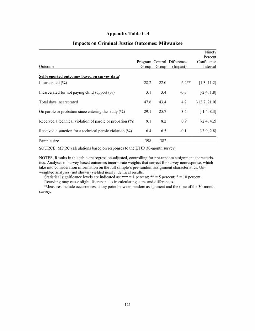
121
Appendix Table C.3
a
Impacts on Criminal Justice Outcomes: Milwaukee
Ninety
Percent Program Control Difference Confidence Outcome Group Group (Impact) Interval
Self-reported outcomes based on survey data Incarcerated (%) 28.2 22.0 6.2 ** [1.3, 11.2]
Incarcerated for not paying child support (%) 3.1 3.4 -0.3 [-2.4, 1.8]
Total days incarcerated 47.6 43.4 4.2 [-12.7, 21.0]
On parole or probation since entering the study (%) 29.1 25.7 3.5 [-1.4, 8.3]
Received a technical violation of parole or probation (%) 9.1 8.2 0.9 [-2.4, 4.2]
Received a sanction for a technical parole violation (%) 6.4 6.5 -0.1 [-3.0, 2.8]
Sample size 398 382
SOURCE: MDRC calculations based on responses to the ETJD 30-month survey.
NOTES: Results in this table are regression-adjusted, controlling for pre-random assignment characteris-tics. Analyses of survey-based outcomes incorporate weights that correct for survey nonresponse, which take into consideration information on the full sample’s pre-random assignment characteristics. Un-weighted analyses (not shown) yielded nearly identical results. Statistical significance levels are indicated as: *** = 1 percent; ** = 5 percent; * = 10 percent. Rounding may cause slight discrepancies in calculating sums and differences. aMeasures include occurrences at any point between random assignment and the time of the 30-month survey.
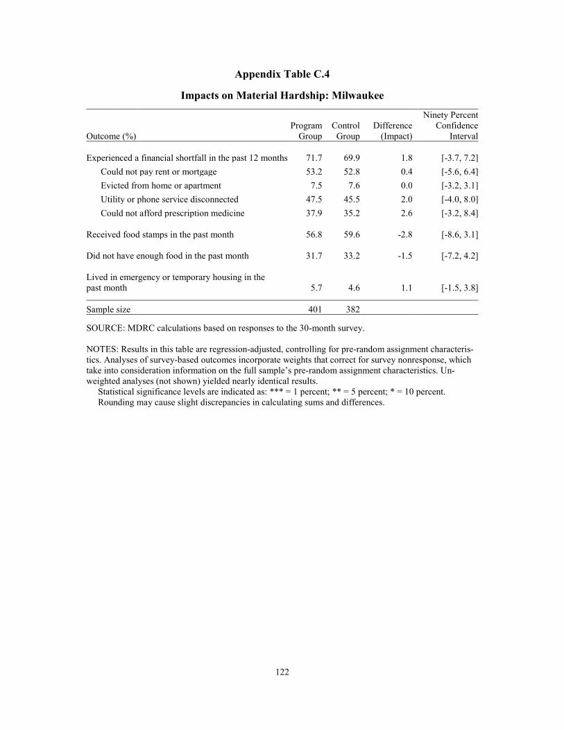
122
Appendix Table C.4
Impacts on Material Hardship: Milwaukee
Ninety Percent Program Control Difference Confidence Outcome (%) Group Group (Impact) Interval
Experienced a financial shortfall in the past 12 months 71.7 69.9 1.8 [-3.7, 7.2] Could not pay rent or mortgage 53.2 52.8 0.4 [-5.6, 6.4] Evicted from home or apartment 7.5 7.6 0.0 [-3.2, 3.1] Utility or phone service disconnected 47.5 45.5 2.0 [-4.0, 8.0] Could not afford prescription medicine 37.9 35.2 2.6 [-3.2, 8.4]
Received food stamps in the past month 56.8 59.6 -2.8 [-8.6, 3.1]
Did not have enough food in the past month 31.7 33.2 -1.5 [-7.2, 4.2]
Lived in emergency or temporary housing in the past month 5.7 4.6 1.1 [-1.5, 3.8]
Sample size 401 382
SOURCE: MDRC calculations based on responses to the 30-month survey.
NOTES: Results in this table are regression-adjusted, controlling for pre-random assignment characteris-tics. Analyses of survey-based outcomes incorporate weights that correct for survey nonresponse, which take into consideration information on the full sample’s pre-random assignment characteristics. Un-weighted analyses (not shown) yielded nearly identical results. Statistical significance levels are indicated as: *** = 1 percent; ** = 5 percent; * = 10 percent. Rounding may cause slight discrepancies in calculating sums and differences.
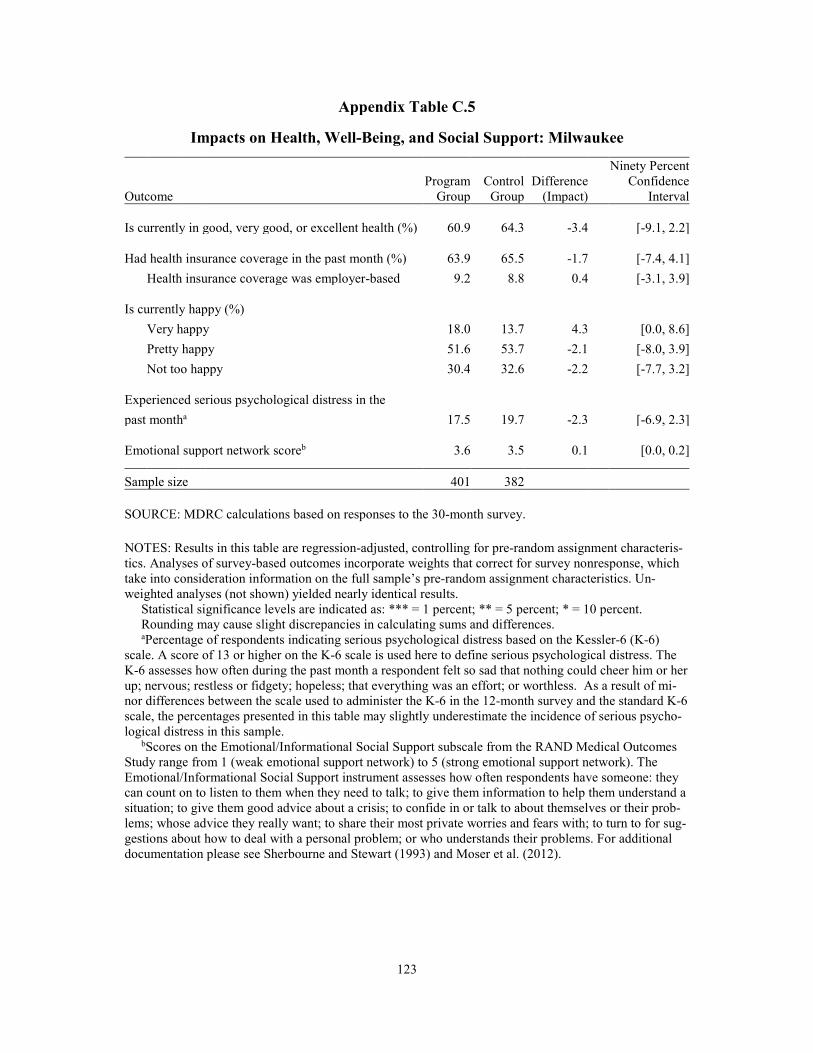
123
Appendix Table C.5
b
Impacts on Health, Well-Being, and Social Support: Milwaukee
Ninety Percent Program Control Difference Confidence Outcome Group Group (Impact) Interval
Is currently in good, very good, or excellent health (%) 60.9 64.3 -3.4 [-9.1, 2.2]
Had health insurance coverage in the past month (%) 63.9 65.5 -1.7 [-7.4, 4.1] Health insurance coverage was employer-based 9.2 8.8 0.4 [-3.1, 3.9]
Is currently happy (%) Very happy 18.0 13.7 4.3 [0.0, 8.6] Pretty happy 51.6 53.7 -2.1 [-8.0, 3.9] Not too happy 30.4 32.6 -2.2 [-7.7, 3.2]
Experienced serious psychological distress in the past montha 17.5 19.7 -2.3 [-6.9, 2.3]
Emotional support network score 3.6 3.5 0.1 [0.0, 0.2]
Sample size 401 382
SOURCE: MDRC calculations based on responses to the 30-month survey.
NOTES: Results in this table are regression-adjusted, controlling for pre-random assignment characteris-tics. Analyses of survey-based outcomes incorporate weights that correct for survey nonresponse, which take into consideration information on the full sample’s pre-random assignment characteristics. Un-weighted analyses (not shown) yielded nearly identical results. Statistical significance levels are indicated as: *** = 1 percent; ** = 5 percent; * = 10 percent. Rounding may cause slight discrepancies in calculating sums and differences. aPercentage of respondents indicating serious psychological distress based on the Kessler-6 (K-6) scale. A score of 13 or higher on the K-6 scale is used here to define serious psychological distress. The K-6 assesses how often during the past month a respondent felt so sad that nothing could cheer him or her up; nervous; restless or fidgety; hopeless; that everything was an effort; or worthless. As a result of mi-nor differences between the scale used to administer the K-6 in the 12-month survey and the standard K-6 scale, the percentages presented in this table may slightly underestimate the incidence of serious psycho-logical distress in this sample. bScores on the Emotional/Informational Social Support subscale from the RAND Medical Outcomes Study range from 1 (weak emotional support network) to 5 (strong emotional support network). The Emotional/Informational Social Support instrument assesses how often respondents have someone: they can count on to listen to them when they need to talk; to give them information to help them understand a situation; to give them good advice about a crisis; to confide in or talk to about themselves or their prob-lems; whose advice they really want; to share their most private worries and fears with; to turn to for sug-gestions about how to deal with a personal problem; or who understands their problems. For additional documentation please see Sherbourne and Stewart (1993) and Moser et al. (2012).
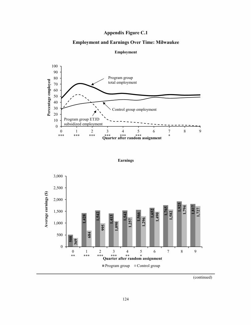
124
(continued)
Appendix Figure C.1
Employment and Earnings Over Time: Milwaukee
Employment
Earnings
0102030405060708090
100
0***
1***
2***
3***
4***
5***
6 7*
8 9
Perc
enta
ge e
mpl
oyed
Quarter after random assignment
Program group total employment
Control group employment
508
1,42
8
1,54
2
1,41
3
1,54
2
1,56
6
1,65
2
1,76
5
1,92
5
1,81
7
369
684
995
1,09
0
1,25
7
1,29
6 1,49
0
1,58
2 1,79
4
1,72
7
0
500
1,000
1,500
2,000
2,500
3,000
0**
1***
2***
3***
4**
5*
6 7 8 9
Ave
rage
ear
ning
s ($)
Quarter after random assignment
Program group Control group
Program group ETJDsubsidized employment

125
Appendix Figure C.1 (continued)
SOURCES: MDRC calculations based on quarterly wage data from the National Directory of New Hiresand program payroll records.
NOTES: Results in this figure are regression-adjusted, controlling for pre-random assignment characteristics.
Statistical significance levels are indicated as: *** = 1 percent; ** = 5 percent; * = 10 percent.Employment rates and earnings in the quarter of random assignment through Quarter 5 after random
assignment include both ETJD subsidized jobs and jobs covered by unemployment insurance and reported to the National Directory of New Hires. Employment rates and earnings in Quarters 6 through 9 after random assignment include only jobs covered by unemployment insurance and reported to the National Directory of New Hires.
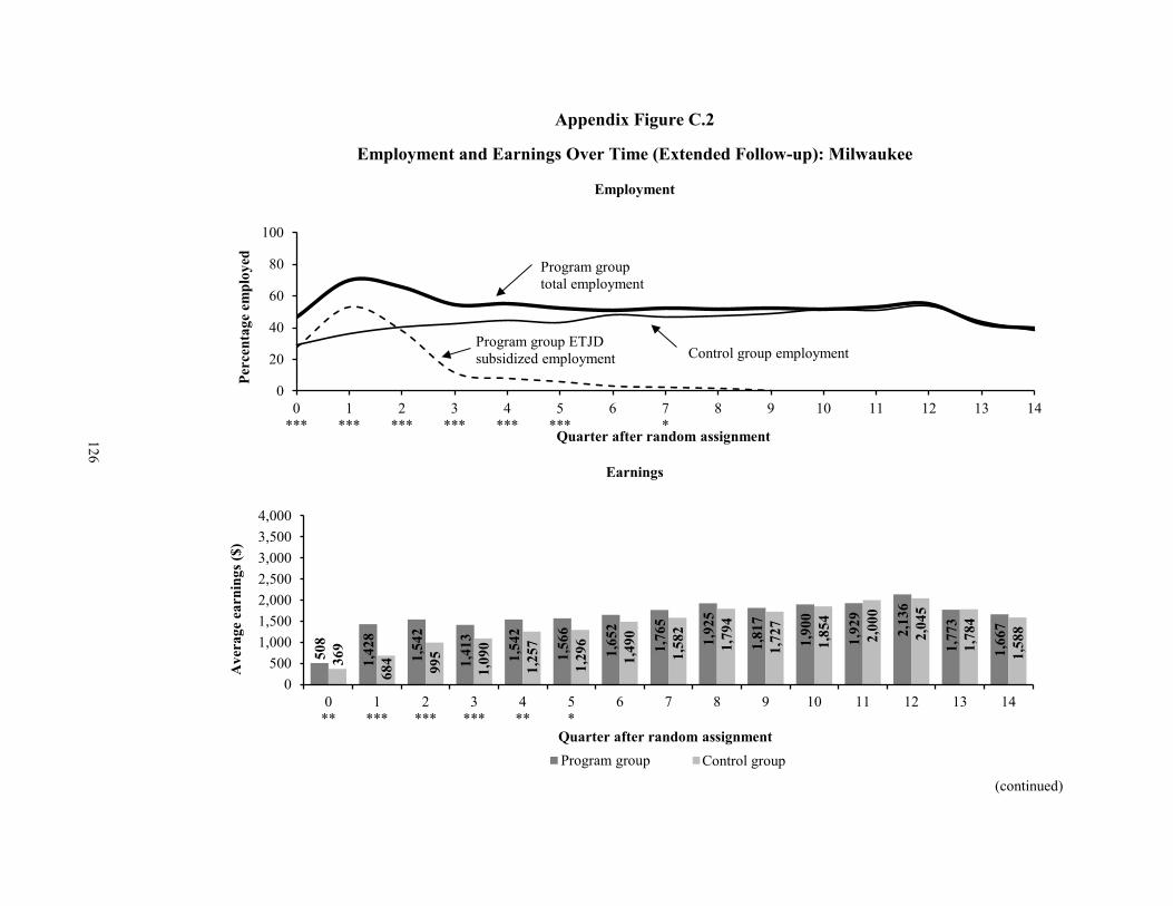
(continued)
Appendix Figure C.2
Employment and Earnings Over Time (Extended Follow-up): Milwaukee
Employment
Earnings
0
20
40
60
80
100
0***
1***
2***
3***
4***
5***
6 7*
8 9 10 11 12 13 14
Perc
enta
ge e
mpl
oyed
Quarter after random assignment
Program group total employment
Control group employment
508
1,42
8
1,54
2
1,41
3
1,54
2
1,56
6
1,65
2
1,76
5
1,92
5
1,81
7
1,90
0
1,92
9
2,13
6
1,77
3
1,66
7
369
684 995
1,09
0
1,25
7
1,29
6
1,49
0
1,58
2
1,79
4
1,72
7
1,85
4
2,00
0
2,04
5
1,78
4
1,58
8
0500
1,0001,5002,0002,5003,0003,5004,000
0**
1***
2***
3***
4**
5*
6 7 8 9 10 11 12 13 14
Ave
rage
ear
ning
s ($)
Quarter after random assignmentProgram group Control GroupControl group
Program group ETJDsubsidized employment
126

127
Appendix Figure C.2 (continued) SOURCES: MDRC calculations based on quarterly wage data from the National Directory of New Hires and program payroll records. NOTES: Results in this figure are regression-adjusted, controlling for pre-random assignment character-istics. Statistical significance levels are indicated as: *** = 1 percent; ** = 5 percent; * = 10 percent. Employment rates and earnings in the quarter of random assignment through Quarter 5 after random assignment include both ETJD subsidized jobs and jobs covered by unemployment insurance and re-ported to the National Directory of New Hires. Employment rates and earnings in Quarters 6 through 14 after random assignment include only jobs covered by unemployment insurance and reported to the Na-tional Directory of New Hires.
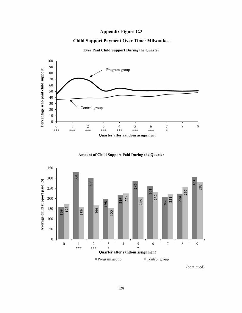
128
(continued)
Appendix Figure C.3
Child Support Payment Over Time: Milwaukee
Ever Paid Child Support During the Quarter
Amount of Child Support Paid During the Quarter
0102030405060708090
100
0***
1***
2***
3***
4***
5***
6***
7*
8 9Perc
enta
ge w
ho p
aid
child
supp
ort
Quarter after random assignment
Program group
Control group
159
331
300
198 21
6
286
261
206 22
4
305
172
159 166
155
225
208 23
2
221
257 28
2
0
50
100
150
200
250
300
350
0 1***
2***
3*
4 5*
6 7 8 9
Ave
rage
chi
ld su
ppor
t pai
d ($
)
Quarter after random assignment
Program group Control group

129
Appendix Figure C.3 (continued)
SOURCE: MDRC calculations based on child support agency data.
NOTES: Results in this figure are regression-adjusted, controlling for pre-random assignment characteristics.
Statistical significance levels are indicated as: *** = 1 percent; ** = 5 percent; * = 10 percent.

THIS PAGE INTENTIONALLY LEFT BLANK

Appendix D
Supplementary Tables and Figures for San Francisco

THIS PAGE INTENTIONALLY LEFT BLANK
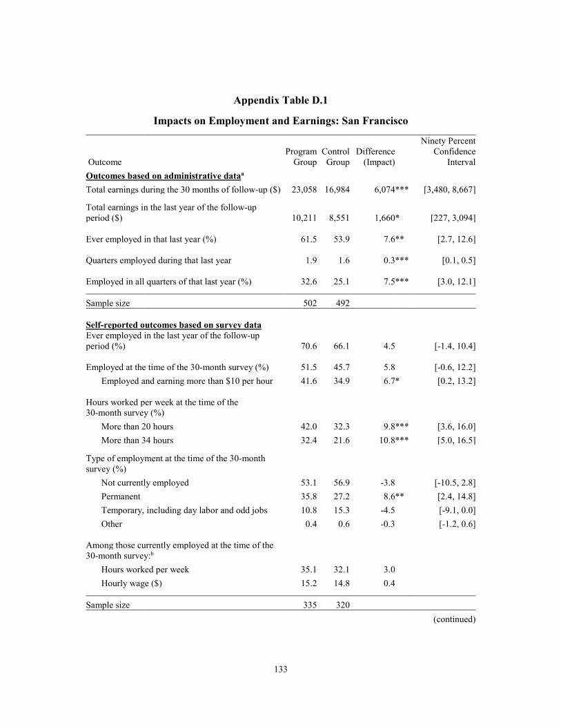
133
Appendix Table D.1
(continued)
Impacts on Employment and Earnings: San Francisco
Outcome Program
Group Control
Group Difference
(Impact)
Ninety Percent Confidence
Interval Outcomes based on administrative dataa Total earnings during the 30 months of follow-up ($) 23,058 16,984 6,074 *** [3,480, 8,667]
Total earnings in the last year of the follow-up period ($) 10,211 8,551 1,660 * [227, 3,094]
Ever employed in that last year (%) 61.5 53.9 7.6 ** [2.7, 12.6]
Quarters employed during that last year 1.9 1.6 0.3 *** [0.1, 0.5]
Employed in all quarters of that last year (%) 32.6 25.1 7.5 *** [3.0, 12.1]
Sample size 502 492
Self-reported outcomes based on survey data Ever employed in the last year of the follow-up period (%) 70.6 66.1 4.5 [-1.4, 10.4]
Employed at the time of the 30-month survey (%) 51.5 45.7 5.8 [-0.6, 12.2] Employed and earning more than $10 per hour 41.6 34.9 6.7 * [0.2, 13.2]
Hours worked per week at the time of the 30-month survey (%)
More than 20 hours 42.0 32.3 9.8 *** [3.6, 16.0] More than 34 hours 32.4 21.6 10.8 *** [5.0, 16.5]
Type of employment at the time of the 30-month survey (%)
Not currently employed 53.1 56.9 -3.8 [-10.5, 2.8] Permanent 35.8 27.2 8.6 ** [2.4, 14.8] Temporary, including day labor and odd jobs 10.8 15.3 -4.5 [-9.1, 0.0] Other 0.4 0.6 -0.3 [-1.2, 0.6]
Among those currently employed at the time of the 30-month survey:b
Hours worked per week 35.1 32.1 3.0 Hourly wage ($) 15.2 14.8 0.4
Sample size 335 320

134
Appendix Table D.1 (continued) SOURCES: MDRC calculations based on quarterly wage data from the National Directory of New Hires and responses to the ETJD 30-month survey. NOTES: Results in this table are regression-adjusted, controlling for pre-random assignment characteris-tics. Analyses of survey-based outcomes incorporate weights that correct for survey nonresponse, which take into consideration information on the full sample’s pre-random assignment characteristics. Un-weighted analyses (not shown) yielded nearly identical results. Statistical significance levels are indicated as: *** = 1 percent; ** = 5 percent; * = 10 percent. Rounding may cause slight discrepancies in calculating sums and differences. aEmployment rates and earnings include only jobs covered by unemployment insurance and reported to the National Directory of New Hires. bThese measures are calculated among those employed at the time of the survey; they are therefore considered nonexperimental and are not tested for statistical significance.
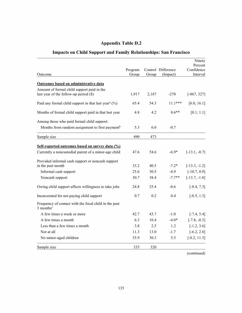
135
Appendix Table D.2
(continued)
Impacts on Child Support and Family Relationships: San Francisco
Ninety
Percent Program Control Difference Confidence Outcome Group Group (Impact) Interval
Outcomes based on administrative data Amount of formal child support paid in the last year of the follow-up period ($) 1,917 2,187 -270 [-867, 327]
Paid any formal child support in that last yeara (%) 65.4 54.3 11.1 *** [6.0, 16.1]
Months of formal child support paid in that last year 4.8 4.2 0.6 ** [0.1, 1.1]
Among those who paid formal child support: Months from random assignment to first paymentb 5.3 6.0 -0.7
Sample size 490 473
Self-reported outcomes based on survey data (%) Currently a noncustodial parent of a minor-age child 47.6 54.6 -6.9 * [-13.1, -0.7]
Provided informal cash support or noncash support in the past month 33.2 40.5 -7.2 * [-13.3, -1.2]
Informal cash support 25.6 30.5 -4.9 [-10.7, 0.9] Noncash support 30.7 38.4 -7.7 ** [-13.7, -1.8]
Owing child support affects willingness to take jobs 24.8 25.4 -0.6 [-8.4, 7.3]
Incarcerated for not paying child support 0.7 0.2 0.4 [-0.5, 1.3]
Frequency of contact with the focal child in the past 3 monthsc
A few times a week or more 42.7 43.7 -1.0 [-7.4, 5.4] A few times a month 6.3 10.4 -4.0 * [-7.8, -0.3] Less than a few times a month 3.8 2.5 1.2 [-1.2, 3.6] Not at all 11.3 13.0 -1.7 [-6.2, 2.8] No minor-aged children 35.9 30.3 5.5 [-0.2, 11.3]
Sample size 335 320

136
Appendix Table D.2 (continued) SOURCES: MDRC calculations based on child support agency data and responses to the ETJD 30-month survey. NOTES: Results in this table are regression-adjusted, controlling for pre-random assignment characteris-tics. Analyses of survey-based outcomes incorporate weights that correct for survey nonresponse, which take into consideration information on the full sample’s pre-random assignment characteristics. Un-weighted analyses (not shown) yielded nearly identical results. Statistical significance levels are indicated as: *** = 1 percent; ** = 5 percent; * = 10 percent. Rounding may cause slight discrepancies in calculating sums and differences. aMeasures of formal child support include all payments made through the state’s child support collec-tion and disbursement unit, including funds from employer withholding and other sources (for example, intercepted tax refunds). bThis measure is calculated among those who paid child support during the follow-up period; it is therefore considered nonexperimental and is not tested for statistical significance. cThe focal child is defined as the youngest minor-age child living outside of the sample member’s household; if the sample member reports no minor-age children living outside of his or her household, the focal child is the youngest minor-age child residing within the household. A contact is defined as spend-ing one or more hours a day with the focal child.
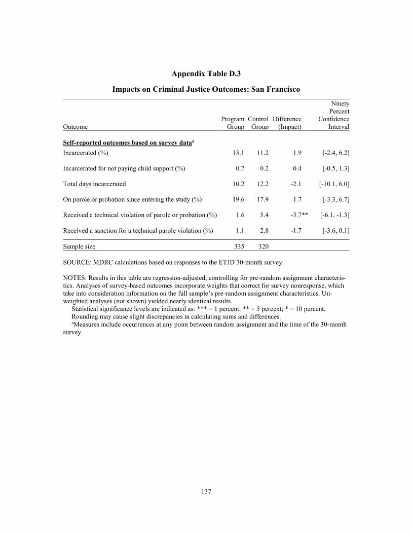
137
Appendix Table D.3
Impacts on Criminal Justice Outcomes: San Francisco
Ninety
Percent Program Control Difference Confidence Outcome Group Group (Impact) Interval
Self-reported outcomes based on survey dataa Incarcerated (%) 13.1 11.2 1.9 [-2.4, 6.2]
Incarcerated for not paying child support (%) 0.7 0.2 0.4 [-0.5, 1.3]
Total days incarcerated 10.2 12.2 -2.1 [-10.1, 6.0]
On parole or probation since entering the study (%) 19.6 17.9 1.7 [-3.3, 6.7]
Received a technical violation of parole or probation (%) 1.6 5.4 -3.7 ** [-6.1, -1.3]
Received a sanction for a technical parole violation (%) 1.1 2.8 -1.7 [-3.6, 0.1]
Sample size 335 320
SOURCE: MDRC calculations based on responses to the ETJD 30-month survey.
NOTES: Results in this table are regression-adjusted, controlling for pre-random assignment characteris-tics. Analyses of survey-based outcomes incorporate weights that correct for survey nonresponse, which take into consideration information on the full sample’s pre-random assignment characteristics. Un-weighted analyses (not shown) yielded nearly identical results. Statistical significance levels are indicated as: *** = 1 percent; ** = 5 percent; * = 10 percent. Rounding may cause slight discrepancies in calculating sums and differences. aMeasures include occurrences at any point between random assignment and the time of the 30-month survey.

138
Appendix Table D.4
Impacts on Material Hardship: San Francisco
Ninety Percent Program Control Difference Confidence Outcome (%) Group Group (Impact) Interval
Experienced a financial shortfall in the past 12 months 45.1 56.4 -11.3 *** [-17.8, -4.8] Could not pay rent or mortgage 32.3 39.9 -7.6 ** [-13.9, -1.3] Evicted from home or apartment 6.8 6.9 -0.1 [-3.4, 3.3] Utility or phone service disconnected 22.3 28.3 -6.0 * [-11.7, -0.4] Could not afford prescription medicine 19.6 27.3 -7.6 ** [-13.1, -2.1]
Received food stamps in the past month 38.0 43.0 -5.0 [-11.2, 1.2]
Did not have enough food in the past month 32.6 35.6 -3.0 [-9.1, 3.2]
Lived in emergency or temporary housing in the past month 6.1 8.2 -2.2 [-5.6, 1.2]
Sample size 335 320
SOURCE: MDRC calculations based on responses to the 30-month survey.
NOTES: Results in this table are regression-adjusted, controlling for pre-random assignment characteris-tics. Analyses of survey-based outcomes incorporate weights that correct for survey nonresponse, which take into consideration information on the full sample’s pre-random assignment characteristics. Un-weighted analyses (not shown) yielded nearly identical results.
Statistical significance levels are indicated as: *** = 1 percent; ** = 5 percent; * = 10 percent. Rounding may cause slight discrepancies in calculating sums and differences.

139
Appendix Table D.5
Impacts on Health, Well-Being, and Social Support: San Francisco
Ninety
Percent Program Control Difference Confidence Outcome Group Group (Impact) Interval
Is currently in good, very good, or excellent health (%) 68.0 63.3 4.7 [-1.5, 10.8]
Had health insurance coverage in the past month (%) 63.8 57.7 6.1 [-0.2, 12.5] Health insurance coverage was employer-based 20.3 12.1 8.2 *** [3.3, 13.1]
Is currently happy (%) Very happy 21.0 21.3 -0.4 [-5.7, 5.0] Pretty happy 59.3 51.6 7.7 * [1.2, 14.2] Not too happy 19.8 27.1 -7.3 ** [-12.8, -1.8]
Experienced serious psychological distress in the past montha 9.8 13.8 -4.0 [-8.2, 0.1]
Emotional support network scoreb 3.5 3.5 0.0 [-0.2, 0.2]
Sample size 335 320
SOURCE: MDRC calculations based on responses to the 30-month survey.
NOTES: Results in this table are regression-adjusted, controlling for pre-random assignment characteris-tics. Analyses of survey-based outcomes incorporate weights that correct for survey nonresponse, which take into consideration information on the full sample’s pre-random assignment characteristics. Un-weighted analyses (not shown) yielded nearly identical results. Statistical significance levels are indicated as: *** = 1 percent; ** = 5 percent; * = 10 percent. Rounding may cause slight discrepancies in calculating sums and differences. aPercentage of respondents indicating serious psychological distress based on the Kessler-6 (K-6) scale. A score of 13 or higher on the K-6 scale is used here to define serious psychological distress. The K-6 assesses how often during the past month a respondent felt so sad that nothing could cheer him or her up; nervous; restless or fidgety; hopeless; that everything was an effort; or worthless. As a result of mi-nor differences between the scale used to administer the K-6 in the 12-month survey and the standard K-6 scale, the percentages presented in this table may slightly underestimate the incidence of serious psycho-logical distress in this sample. bScores on the Emotional/Informational Social Support subscale from the RAND Medical Outcomes Study range from 1 (weak emotional support network) to 5 (strong emotional support network). The Emotional/Informational Social Support instrument assesses how often respondents have someone: they can count on to listen to them when they need to talk; to give them information to help them understand a situation; to give them good advice about a crisis; to confide in or talk to about themselves or their prob-lems; whose advice they really want; to share their most private worries and fears with; to turn to for sug-gestions about how to deal with a personal problem; or who understands their problems. For additional documentation please see Sherbourne and Stewart (1993) and Moser et al. (2012).
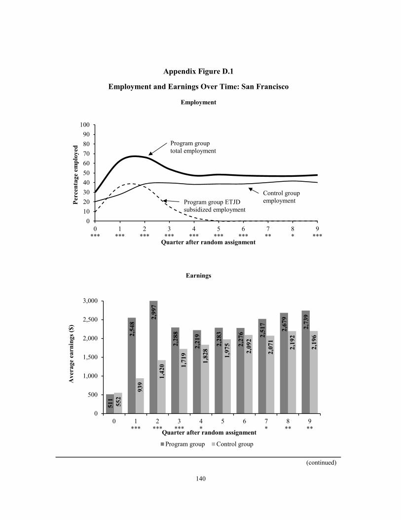
140
(continued)
Appendix Figure D.1
Employment and Earnings Over Time: San Francisco
Employment
Earnings
0102030405060708090
100
0***
1***
2***
3***
4***
5***
6***
7**
8*
9***
Perc
enta
ge e
mpl
oyed
Quarter after random assignment
Program group total employment
Control group employment
511
2,54
8
2,99
7
2,28
8
2,21
9
2,28
3
2,27
6 2,51
7
2,67
9
2,73
9
552
939
1,42
0 1,71
9
1,82
8
1,97
5
2,09
2
2,07
1
2,19
2
2,19
6
0
500
1,000
1,500
2,000
2,500
3,000
0 1***
2***
3***
4*
5 6 7*
8**
9**
Ave
rage
ear
ning
s ($)
Quarter after random assignment
Program group Control group
Program group ETJD subsidized employment

141
Appendix Figure D.1 (continued)
SOURCES: MDRC calculations based on quarterly wage data from the National Directory of New Hiresand program payroll records.
NOTES: Results in this figure are regression-adjusted, controlling for pre-random assignment characteristics.
Statistical significance levels are indicated as: *** = 1 percent; ** = 5 percent; * = 10 percent.Employment rates and earnings in the quarter of random assignment through Quarter 5 after random
assignment include both ETJD subsidized jobs and jobs covered by unemployment insurance and reported to the National Directory of New Hires. Employment rates and earnings in Quarters 6 through 9 after random assignment include only jobs covered by unemployment insurance and reported to the National Directory of New Hires.
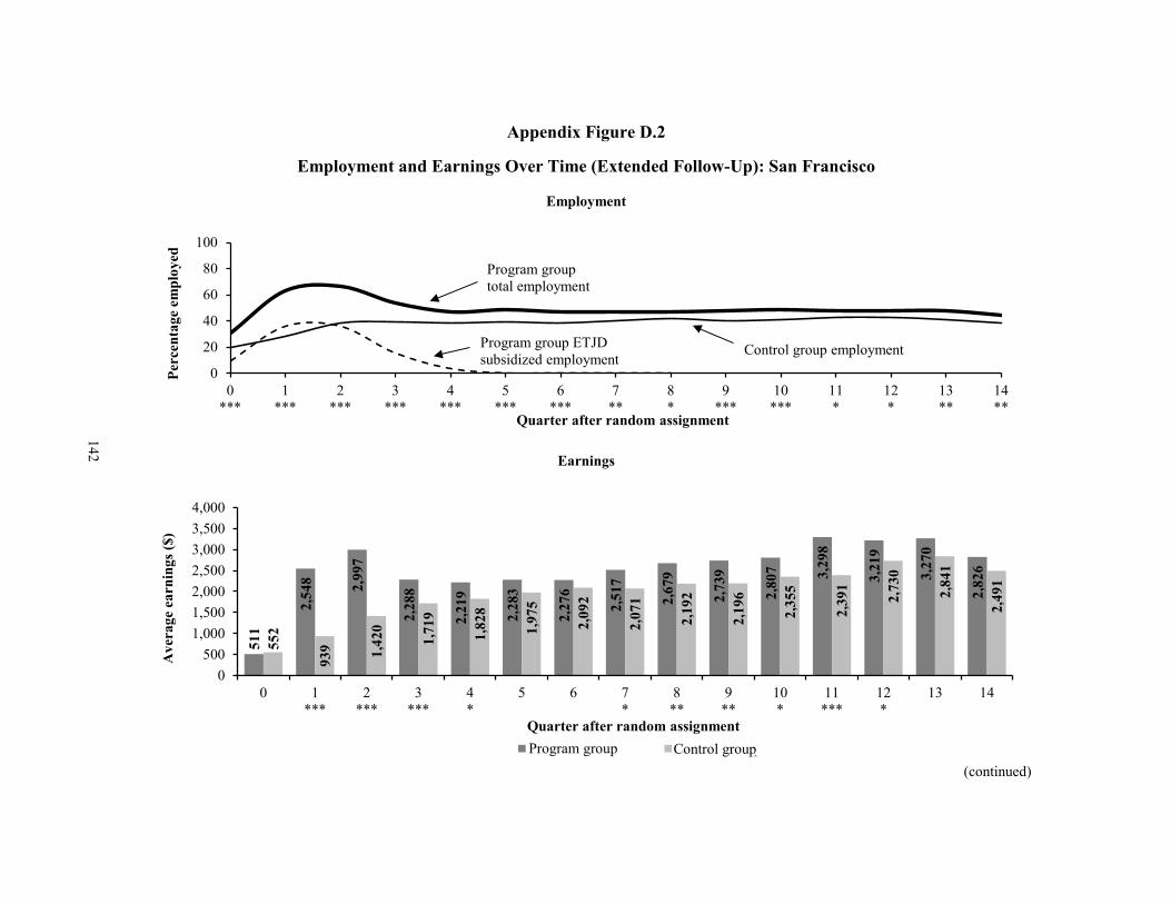
(continued)
Appendix Figure D.2
Employment and Earnings Over Time (Extended Follow-Up): San Francisco
Employment
Earnings
0
20
40
60
80
100
0***
1***
2***
3***
4***
5***
6***
7**
8*
9***
10***
11*
12*
13**
14**
Perc
enta
ge e
mpl
oyed
Quarter after random assignment
Program group total employment
Control group employment
511
2,54
8 2,99
7
2,28
8
2,21
9
2,28
3
2,27
6
2,51
7
2,67
9
2,73
9
2,80
7 3,29
8
3,21
9
3,27
0
2,82
6
552
939 1,42
0
1,71
9
1,82
8
1,97
5
2,09
2
2,07
1
2,19
2
2,19
6
2,35
5
2,39
1
2,73
0
2,84
1
2,49
1
0500
1,0001,5002,0002,5003,0003,5004,000
0 1***
2***
3***
4*
5 6 7*
8**
9**
10*
11***
12*
13 14
Ave
rage
ear
ning
s ($)
Quarter after random assignmentProgram group Control GroupControl group
Program group ETJDsubsidized employment
142

143
Appendix Figure D.2 (continued) SOURCES: MDRC calculations based on quarterly wage data from the National Directory of New Hires and program payroll records. NOTES: Results in this figure are regression-adjusted, controlling for pre-random assignment character-istics. Statistical significance levels are indicated as: *** = 1 percent; ** = 5 percent; * = 10 percent. Employment rates and earnings in the quarter of random assignment through Quarter 5 after random assignment include both ETJD subsidized jobs and jobs covered by unemployment insurance and re-ported to the National Directory of New Hires. Employment rates and earnings in Quarters 6 through 14 after random assignment include only jobs covered by unemployment insurance and reported to the Na-tional Directory of New Hires.
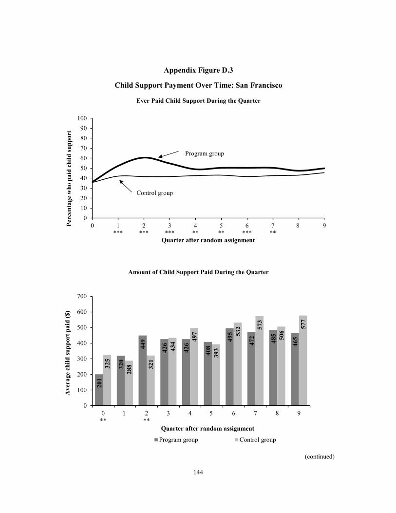
144
(continued)
Appendix Figure D.3
Child Support Payment Over Time: San Francisco
Ever Paid Child Support During the Quarter
Amount of Child Support Paid During the Quarter
0102030405060708090
100
0 1***
2***
3***
4**
5**
6***
7**
8 9Perc
enta
ge w
ho p
aid
child
supp
ort
Quarter after random assignment
Program group
Control group
201
320
449
426
426
408
495
472
485
465
325
288 32
1
434 49
7
393
532 57
3
506
577
0
100
200
300
400
500
600
700
0**
1 2**
3 4 5 6 7 8 9
Ave
rage
chi
ld su
ppor
t pai
d ($
)
Quarter after random assignment
Program group Control group

145
Appendix Figure D.3 (continued)
SOURCE: MDRC calculations based on child support agency data.
NOTES: Results in this figure are regression-adjusted, controlling for pre-random assignment characteristics.
Statistical significance levels are indicated as: *** = 1 percent; ** = 5 percent; * = 10 percent.

THIS PAGE INTENTIONALLY LEFT BLANK

Appendix E
Supplementary Tables and Figures for Syracuse

THIS PAGE INTENTIONALLY LEFT BLANK
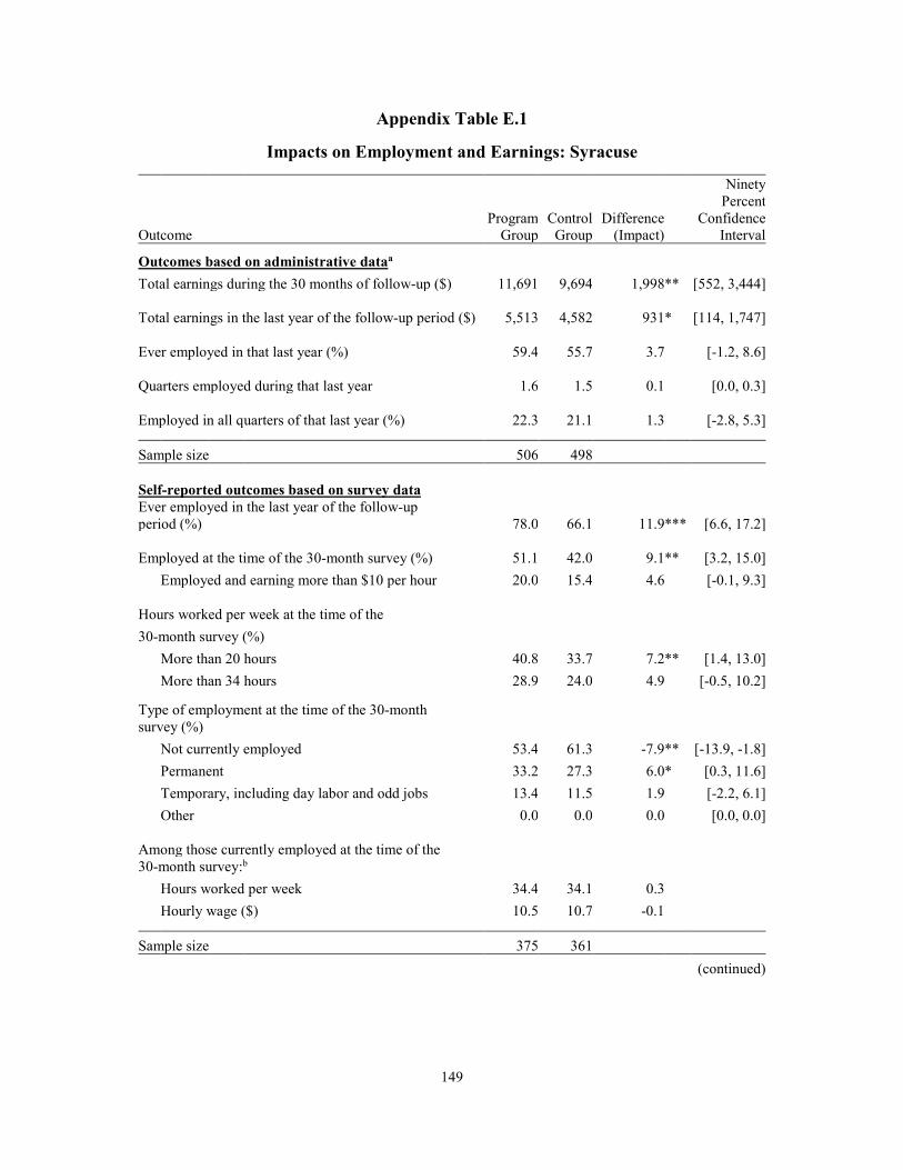
149
Appendix Table E.1
(continued)
Impacts on Employment and Earnings: Syracuse
Outcome Program
Group Control
Group Difference
(Impact)
Ninety Percent
Confidence Interval
Outcomes based on administrative dataa Total earnings during the 30 months of follow-up ($) 11,691 9,694 1,998 ** [552, 3,444]
Total earnings in the last year of the follow-up period ($) 5,513 4,582 931 * [114, 1,747]
Ever employed in that last year (%) 59.4 55.7 3.7 [-1.2, 8.6]
Quarters employed during that last year 1.6 1.5 0.1 [0.0, 0.3]
Employed in all quarters of that last year (%) 22.3 21.1 1.3 [-2.8, 5.3]
Sample size 506 498
Self-reported outcomes based on survey data Ever employed in the last year of the follow-up period (%) 78.0 66.1 11.9 *** [6.6, 17.2]
Employed at the time of the 30-month survey (%) 51.1 42.0 9.1 ** [3.2, 15.0] Employed and earning more than $10 per hour 20.0 15.4 4.6 [-0.1, 9.3]
Hours worked per week at the time of the 30-month survey (%)
More than 20 hours 40.8 33.7 7.2 ** [1.4, 13.0] More than 34 hours 28.9 24.0 4.9 [-0.5, 10.2]
Type of employment at the time of the 30-month survey (%)
Not currently employed 53.4 61.3 -7.9 ** [-13.9, -1.8] Permanent 33.2 27.3 6.0 * [0.3, 11.6] Temporary, including day labor and odd jobs 13.4 11.5 1.9 [-2.2, 6.1] Other 0.0 0.0 0.0 [0.0, 0.0]
Among those currently employed at the time of the 30-month survey:b
Hours worked per week 34.4 34.1 0.3 Hourly wage ($) 10.5 10.7 -0.1
Sample size 375 361

150
Appendix Table E.1 (continued)
SOURCES: MDRC calculations based on quarterly wage data from the National Directory of New Hires and responses to the ETJD 30-month survey. NOTES: Results in this table are regression-adjusted, controlling for pre-random assignment characteris-tics. Analyses of survey-based outcomes incorporate weights that correct for survey nonresponse, which take into consideration information on the full sample’s pre-random assignment characteristics. Un-weighted analyses (not shown) yielded nearly identical results. Statistical significance levels are indicated as: *** = 1 percent; ** = 5 percent; * = 10 percent. Rounding may cause slight discrepancies in calculating sums and differences. aEmployment rates and earnings include only jobs covered by unemployment insurance and reported to the National Directory of New Hires. bThese measures are calculated among those employed at the time of the survey; they are therefore considered nonexperimental and are not tested for statistical significance.

151
Appendix Table E.2
(continued)
Impacts on Child Support and Family Relationships: Syracuse
Ninety
Percent Program Control Difference Confidence Outcome Group Group (Impact) Interval
Outcomes based on administrative data Amount of formal child support paid in the last year of the follow-up period ($) 338 310 27 [-78, 132]
Paid any formal child support in that last yeara (%) 36.3 28.6 7.7 *** [2.9, 12.5]
Months of formal child support paid in that last year 2.4 1.7 0.7 *** [0.3, 1.1]
Among those who paid formal child support: Months from random assignment to first paymentb 7.5 8.6 -1.2
Sample size 506 498
Self-reported outcomes based on survey data (%) Currently a noncustodial parent of a minor-age child 79.7 75.1 4.5 [-0.4, 9.4]
Provided informal cash support or noncash support in the past month 55.8 51.3 4.4 [-1.5, 10.4]
Informal cash support 44.6 37.6 7.0 ** [1.2, 12.8] Noncash support 52.8 49.2 3.5 [-2.4, 9.5]
Owing child support affects willingness to take jobs 21.2 19.9 1.3 [-4.3, 6.8]
Incarcerated for not paying child support 1.7 2.7 -0.9 [-2.8, 0.9]
Frequency of contact with the focal child in the past 3 monthsc
A few times a week or more 47.3 44.9 2.4 [-3.6, 8.5] A few times a month 10.6 10.6 0.0 [-3.9, 3.8] Less than a few times a month 6.6 4.3 2.4 [-0.5, 5.2] Not at all 26.1 26.5 -0.4 [-5.8, 5.1] No minor-aged children 9.3 13.7 -4.4 * [-8.1, -0.7]
Sample size 375 361

152
Appendix Table E.2 (continued) SOURCES: MDRC calculations based on child support agency data and responses to the ETJD 30-month survey. NOTES: Results in this table are regression-adjusted, controlling for pre-random assignment characteris-tics. Analyses of survey-based outcomes incorporate weights that correct for survey nonresponse, which take into consideration information on the full sample’s pre-random assignment characteristics. Un-weighted analyses (not shown) yielded nearly identical results. Statistical significance levels are indicated as: *** = 1 percent; ** = 5 percent; * = 10 percent. Rounding may cause slight discrepancies in calculating sums and differences. aMeasures of formal child support include all payments made through the state’s child support collec-tion and disbursement unit, including funds from employer withholding and other sources (for example, intercepted tax refunds). bThis measure is calculated among those who paid child support during the follow-up period; it is therefore considered nonexperimental and is not tested for statistical significance. cThe focal child is defined as the youngest minor-age child living outside of the sample member’s household; if the sample member reports no minor-age children living outside of his or her household, the focal child is the youngest minor-age child residing within the household. A contact is defined as spend-ing one or more hours a day with the focal child.
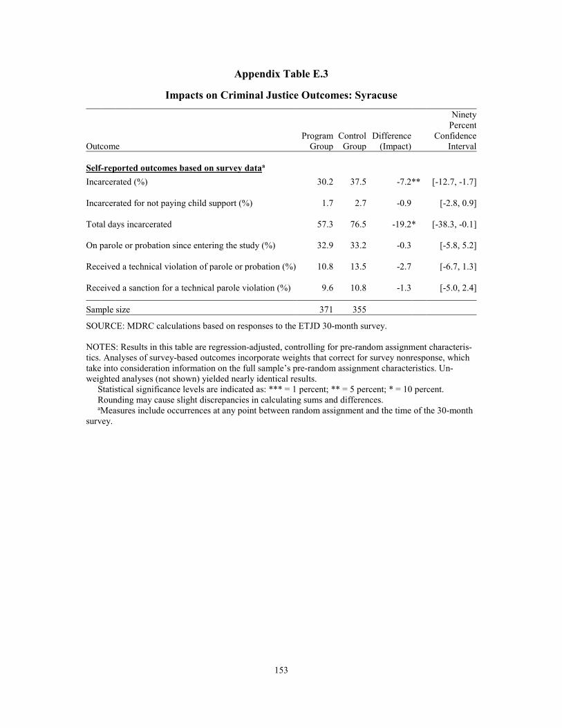
153
Appendix Table E.3
Impacts on Criminal Justice Outcomes: Syracuse
a
Ninety
Percent Program Control Difference Confidence Outcome Group Group (Impact) Interval
Self-reported outcomes based on survey data Incarcerated (%) 30.2 37.5 -7.2 ** [-12.7, -1.7]
Incarcerated for not paying child support (%) 1.7 2.7 -0.9 [-2.8, 0.9]
Total days incarcerated 57.3 76.5 -19.2 * [-38.3, -0.1]
On parole or probation since entering the study (%) 32.9 33.2 -0.3 [-5.8, 5.2]
Received a technical violation of parole or probation (%) 10.8 13.5 -2.7 [-6.7, 1.3]
Received a sanction for a technical parole violation (%) 9.6 10.8 -1.3 [-5.0, 2.4]
Sample size 371 355
SOURCE: MDRC calculations based on responses to the ETJD 30-month survey.
NOTES: Results in this table are regression-adjusted, controlling for pre-random assignment characteris-tics. Analyses of survey-based outcomes incorporate weights that correct for survey nonresponse, which take into consideration information on the full sample’s pre-random assignment characteristics. Un-weighted analyses (not shown) yielded nearly identical results. Statistical significance levels are indicated as: *** = 1 percent; ** = 5 percent; * = 10 percent. Rounding may cause slight discrepancies in calculating sums and differences. aMeasures include occurrences at any point between random assignment and the time of the 30-month survey.
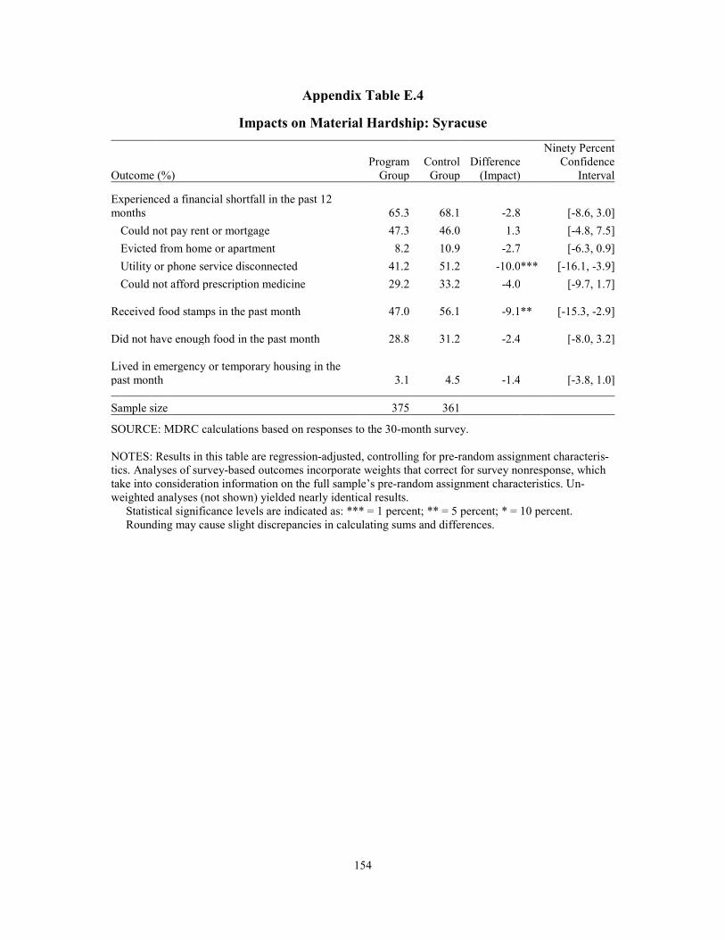
154
Appendix Table E.4
Impacts on Material Hardship: Syracuse
Ninety Percent Program Control Difference Confidence Outcome (%) Group Group (Impact) Interval
Experienced a financial shortfall in the past 12 months 65.3 68.1 -2.8 [-8.6, 3.0]
Could not pay rent or mortgage 47.3 46.0 1.3 [-4.8, 7.5] Evicted from home or apartment 8.2 10.9 -2.7 [-6.3, 0.9] Utility or phone service disconnected 41.2 51.2 -10.0 *** [-16.1, -3.9] Could not afford prescription medicine 29.2 33.2 -4.0 [-9.7, 1.7]
Received food stamps in the past month 47.0 56.1 -9.1 ** [-15.3, -2.9]
Did not have enough food in the past month 28.8 31.2 -2.4 [-8.0, 3.2]
Lived in emergency or temporary housing in the past month 3.1 4.5 -1.4 [-3.8, 1.0]
Sample size 375 361
SOURCE: MDRC calculations based on responses to the 30-month survey.
NOTES: Results in this table are regression-adjusted, controlling for pre-random assignment characteris-tics. Analyses of survey-based outcomes incorporate weights that correct for survey nonresponse, which take into consideration information on the full sample’s pre-random assignment characteristics. Un-weighted analyses (not shown) yielded nearly identical results. Statistical significance levels are indicated as: *** = 1 percent; ** = 5 percent; * = 10 percent. Rounding may cause slight discrepancies in calculating sums and differences.

155
Appendix Table E.5
Impacts on Health, Well-Being, and Social Support: Syracuse
Ninety Percent Program Control Difference Confidence Outcome Group Group (Impact) Interval
Is currently in good, very good, or excellent health (%) 73.8 65.6 8.2 ** [2.7, 13.7]
Had health insurance coverage in the past month (%) 66.7 63.2 3.5 [-2.3, 9.4] Health insurance coverage was employer-based 10.8 5.3 5.4 *** [2.1, 8.7]
Is currently happy (%) Very happy 14.1 13.2 0.9 [-3.4, 5.1] Pretty happy 59.3 58.1 1.2 [-4.8, 7.3] Not too happy 26.6 28.7 -2.1 [-7.6, 3.3]
Experienced serious psychological distress in the past montha 17.5 20.0 -2.5 [-7.2, 2.3]
Emotional support network scoreb 3.7 3.6 0.1 [0.0, 0.2]
Sample size 375 361
SOURCE: MDRC calculations based on responses to the 30-month survey.
NOTES: Results in this table are regression-adjusted, controlling for pre-random assignment characteris-tics. Analyses of survey-based outcomes incorporate weights that correct for survey nonresponse, which take into consideration information on the full sample’s pre-random assignment characteristics. Un-weighted analyses (not shown) yielded nearly identical results. Statistical significance levels are indicated as: *** = 1 percent; ** = 5 percent; * = 10 percent. Rounding may cause slight discrepancies in calculating sums and differences. aPercentage of respondents indicating serious psychological distress based on the Kessler-6 (K-6) scale. A score of 13 or higher on the K-6 scale is used here to define serious psychological distress. The K-6 assesses how often during the past month a respondent felt so sad that nothing could cheer him or her up; nervous; restless or fidgety; hopeless; that everything was an effort; or worthless. As a result of minor differences between the scale used to administer the K-6 in the 12-month survey and the standard K-6 scale, the percentages presented in this table may slightly underestimate the incidence of serious psycho-logical distress in this sample. bScores on the Emotional/Informational Social Support subscale from the RAND Medical Outcomes Study range from 1 (weak emotional support network) to 5 (strong emotional support network). The Emotional/Informational Social Support instrument assesses how often respondents have someone: they can count on to listen to them when they need to talk; to give them information to help them understand a situation; to give them good advice about a crisis; to confide in or talk to about themselves or their prob-lems; whose advice they really want; to share their most private worries and fears with; to turn to for sug-gestions about how to deal with a personal problem; or who understands their problems. For additional documentation please see Sherbourne and Stewart (1993) and Moser et al. (2012).
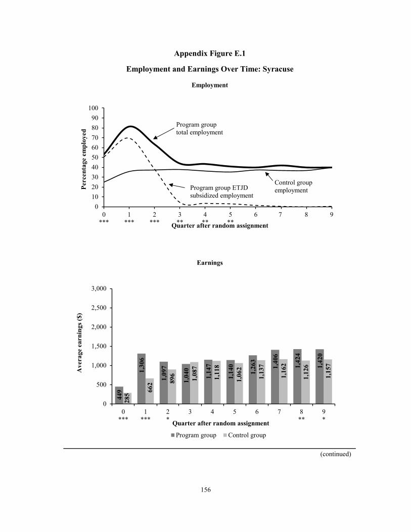
156
(continued)
Appendix Figure E.1
Employment and Earnings Over Time: Syracuse
Employment
Earnings
0102030405060708090
100
0***
1***
2***
3**
4**
5**
6 7 8 9
Perc
enta
ge e
mpl
oyed
Quarter after random assignment
Program group total employment
Control group employment
449
1,30
6
1,09
7
1,04
0
1,14
7
1,14
0
1,26
3
1,40
6
1,42
4
1,42
0
285 66
2 896
1,08
7
1,11
8
1,06
2
1,13
7
1,16
2
1,12
6
1,15
7
0
500
1,000
1,500
2,000
2,500
3,000
0***
1***
2*
3 4 5 6 7 8**
9*
Ave
rage
ear
ning
s ($)
Quarter after random assignment
Program group Control group
Program group ETJDsubsidized employment

157
Appendix Figure E.1 (continued)
SOURCES: MDRC calculations based on quarterly wage data from the National Directory of New Hiresand program payroll records.
NOTES: Results in this figure are regression-adjusted, controlling for pre-random assignment characteristics.
Statistical significance levels are indicated as: *** = 1 percent; ** = 5 percent; * = 10 percent.Employment rates and earnings in the quarter of random assignment through Quarter 5 after random
assignment include both ETJD subsidized jobs and jobs covered by unemployment insurance and reported to the National Directory of New Hires. Employment rates and earnings in Quarters 6 through 9 after random assignment include only jobs covered by unemployment insurance and reported to the National Directory of New Hires.
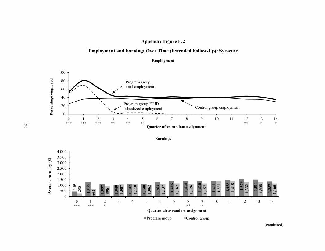
(continued)
Appendix Figure E.2
Employment and Earnings Over Time (Extended Follow-Up): Syracuse
Employment
Earnings
0
20
40
60
80
100
0***
1***
2***
3**
4**
5**
6 7 8 9 10 11 12**
13*
14*
Perc
enta
ge e
mpl
oyed
Quarter after random assignment
Program group total employment
Control group employment
449
1,30
6
1,09
7
1,04
0
1,14
7
1,14
0
1,26
3
1,40
6
1,42
4
1,42
0
1,41
1
1,45
8
1,57
9
1,51
1
1,35
7
285
662 896
1,08
7
1,11
8
1,06
2
1,13
7
1,16
2
1,12
6
1,15
7
1,38
2
1,41
8
1,33
2
1,33
8
1,16
0
0500
1,0001,5002,0002,5003,0003,5004,000
0***
1***
2*
3 4 5 6 7 8**
9*
10 11 12 13 14
Ave
rage
ear
ning
s ($)
Quarter after random assignment
Program group Control GroupControl group
Program group ETJDsubsidized employment
158

159
Appendix Figure E.2 (continued) SOURCES: MDRC calculations based on quarterly wage data from the National Directory of New Hires and program payroll records. NOTES: Results in this figure are regression-adjusted, controlling for pre-random assignment character-istics. Statistical significance levels are indicated as: *** = 1 percent; ** = 5 percent; * = 10 percent. Employment rates and earnings in the quarter of random assignment through Quarter 5 after random assignment include both ETJD subsidized jobs and jobs covered by unemployment insurance and re-ported to the National Directory of New Hires. Employment rates and earnings in Quarters 6 through 14 after random assignment include only jobs covered by unemployment insurance and reported to the Na-tional Directory of New Hires.
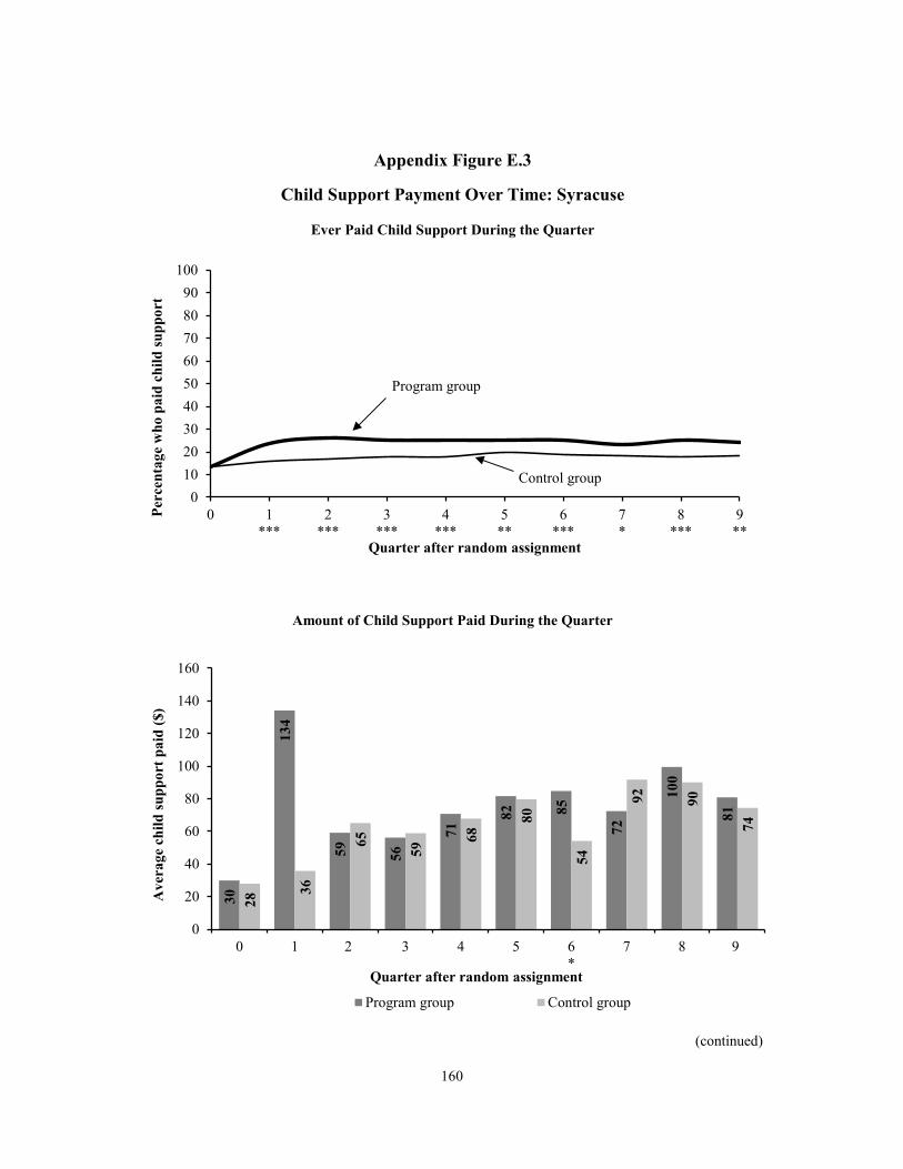
160
(continued)
Appendix Figure E.3
Child Support Payment Over Time: Syracuse
Ever Paid Child Support During the Quarter
Amount of Child Support Paid During the Quarter
0102030405060708090
100
0 1***
2***
3***
4***
5**
6***
7*
8***
9**
Perc
enta
ge w
ho p
aid
child
supp
ort
Quarter after random assignment
Program group
Control group
30
134
59 56
71
82 85
72
100
81
28
36
65
59
68
80
54
92 90
74
0
20
40
60
80
100
120
140
160
0 1 2 3 4 5 6*
7 8 9
Ave
rage
chi
ld su
ppor
t pai
d ($
)
Quarter after random assignment
Program group Control group

161
Appendix Figure E.3 (continued)
SOURCE: MDRC calculations based on child support agency data.
NOTES: Results in this figure are regression-adjusted, controlling for pre-random assignment characteristics.
Statistical significance levels are indicated as: *** = 1 percent; ** = 5 percent; * = 10 percent.

THIS PAGE INTENTIONALLY LEFT BLANK

Appendix F
Supplementary Tables and Figures for Fort Worth

THIS PAGE INTENTIONALLY LEFT BLANK
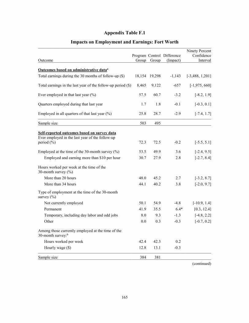
165
Appendix Table F.1
(continued)
Impacts on Employment and Earnings: Fort Worth
Outcome Program
Group Control
Group Difference
(Impact)
Ninety Percent Confidence
Interval
Outcomes based on administrative dataa Total earnings during the 30 months of follow-up ($) 18,154 19,298 -1,143 [-3,488, 1,201]
Total earnings in the last year of the follow-up period ($) 8,465 9,122 -657 [-1,975, 660]
Ever employed in that last year (%) 57.5 60.7 -3.2 [-8.2, 1.9]
Quarters employed during that last year 1.7 1.8 -0.1 [-0.3, 0.1]
Employed in all quarters of that last year (%) 25.8 28.7 -2.9 [-7.4, 1.7]
Sample size 503 495
Self-reported outcomes based on survey data Ever employed in the last year of the follow-up period (%) 72.3 72.5 -0.2 [-5.5, 5.1]
Employed at the time of the 30-month survey (%) 53.5 49.9 3.6 [-2.4, 9.5] Employed and earning more than $10 per hour 30.7 27.9 2.8 [-2.7, 8.4]
Hours worked per week at the time of the 30-month survey (%)
More than 20 hours 48.0 45.2 2.7 [-3.2, 8.7] More than 34 hours 44.1 40.2 3.8 [-2.0, 9.7]
Type of employment at the time of the 30-month survey (%)
Not currently employed 50.1 54.9 -4.8 [-10.9, 1.4] Permanent 41.9 35.5 6.4 * [0.3, 12.4] Temporary, including day labor and odd jobs 8.0 9.3 -1.3 [-4.8, 2.2] Other 0.0 0.3 -0.3 [-0.7, 0.2]
Among those currently employed at the time of the 30-month survey:b
Hours worked per week 42.4 42.3 0.2 Hourly wage ($) 12.8 13.1 -0.3
Sample size 384 381

166
Appendix Table F.1 (continued) SOURCES: MDRC calculations based on quarterly wage data from the National Directory of New Hires and responses to the ETJD 30-month survey. NOTES: Results in this table are regression-adjusted, controlling for pre-random assignment characteris-tics. Analyses of survey-based outcomes incorporate weights that correct for survey nonresponse, which take into consideration information on the full sample’s pre-random assignment characteristics. Un-weighted analyses (not shown) yielded nearly identical results. Statistical significance levels are indicated as: *** = 1 percent; ** = 5 percent; * = 10 percent. Rounding may cause slight discrepancies in calculating sums and differences. aEmployment rates and earnings include only jobs covered by unemployment insurance and reported to the National Directory of New Hires. bThese measures are calculated among those employed at the time of the survey; they are therefore considered nonexperimental and are not tested for statistical significance.
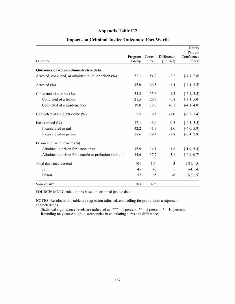
167
Appendix Table F.2
Impacts on Criminal Justice Outcomes: Fort Worth
Outcome Program
Group Control
Group Difference
(Impact)
Ninety Percent
Confidence Interval
Outcomes based on administrative data Arrested, convicted, or admitted to jail or prison (%) 52.1 54.2 -2.2 [-7.1, 2.8]
Arrested (%) 45.0 46.5 -1.4 [-6.4, 3.5]
Convicted of a crime (%) 34.3 35.6 -1.3 [-6.1, 3.5] Convicted of a felony 21.5 20.7 0.8 [-3.4, 5.0] Convicted of a misdemeanor 19.0 19.0 -0.1 [-4.1, 4.0]
Convicted of a violent crime (%) 5.5 6.5 -1.0 [-3.5, 1.4]
Incarcerated (%) 47.1 46.6 0.5 [-4.5, 5.5] Incarcerated in jail 42.2 41.3 1.0 [-4.0, 5.9] Incarcerated in prison 27.6 29.4 -1.8 [-6.4, 2.8]
Prison admission reason (%) Admitted to prison for a new crime 15.9 14.1 1.8 [-1.9, 5.4] Admitted to prison for a parole or probation violation 14.6 17.7 -3.1 [-6.9, 0.7]
Total days incarcerated 101 104 -3 [-21, 15] Jail 45 40 5 [-4, 14] Prison 57 65 -8 [-21, 5]
Sample size 503 496
SOURCE: MDRC calculations based on criminal justice data.
NOTES: Results in this table are regression-adjusted, controlling for pre-random assignment characteristics. Statistical significance levels are indicated as: *** = 1 percent; ** = 5 percent; * = 10 percent. Rounding may cause slight discrepancies in calculating sums and differences.
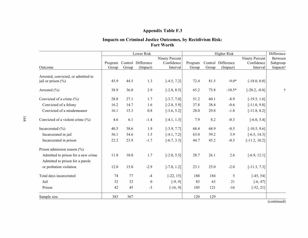
Appendix Table F.3
(continued)
Impacts on Criminal Justice Outcomes, by Recidivism Risk: Fort Worth
Lower Risk Higher Risk Difference
Ninety Percent Ninety Percent Between
Program Control Difference Confidence Program Control Difference Confidence Subgroup Outcome Group Group (Impact) Interval Group Group (Impact) Interval Impactsa
Arrested, convicted, or admitted to jail or prison (%) 45.9 44.5 1.3 [-4.5, 7.2] 72.4 81.5 -9.0 * [-18.0, 0.0]
Arrested (%) 38.9 36.0 2.9 [-2.8, 8.5] 65.2 75.8 -10.5 * [-20.2, -0.8] †
Convicted of a crime (%) 28.8 27.1 1.7 [-3.7, 7.0] 51.2 60.1 -8.9 [-19.5, 1.6] Convicted of a felony 16.2 14.7 1.6 [-2.8, 5.9] 37.8 38.4 -0.6 [-11.0, 9.8] Convicted of a misdemeanor 16.1 15.3 0.8 [-3.6, 5.2] 28.0 29.8 -1.8 [-11.8, 8.2]
Convicted of a violent crime (%) 4.6 6.1 -1.4 [-4.1, 1.3] 7.9 8.2 -0.3 [-6.0, 5.4]
Incarcerated (%) 40.5 38.6 1.9 [-3.9, 7.7] 68.4 68.9 -0.5 [-10.5, 9.6] Incarcerated in jail 36.1 34.6 1.5 [-4.1, 7.2] 63.0 59.2 3.9 [-6.5, 14.3] Incarcerated in prison 22.2 23.9 -1.7 [-6.7, 3.3] 44.7 45.2 -0.5 [-11.2, 10.2]
Prison admission reason (%) Admitted to prison for a new crime 11.8 10.0 1.7 [-2.0, 5.5] 28.7 26.1 2.6 [-6.9, 12.1] Admitted to prison for a parole or probation violation 12.0 15.0 -2.9 [-7.0, 1.2] 23.1 25.0 -2.0 [-11.3, 7.3]
Total days incarcerated 74 77 -4 [-22, 15] 188 184 5 [-45, 54] Jail 32 32 0 [-9, 9] 83 63 21 [-6, 47] Prison 42 45 -3 [-16, 9] 105 121 -16 [-52, 21]
Sample size 383 367 120 129
168

169
Appendix Table F.3 (continued) SOURCE: MDRC calculations based on criminal justice records. NOTES: Results in this table are regression-adjusted, controlling for pre-random assignment characteristics. Statistical significance levels are indicated as: *** = 1 percent; ** = 5 percent; * = 10 percent. Rounding may cause slight discrepancies in calculating sums and differences. See Appendix L for details on how risk of recidivism was defined. aWhen comparing impacts between two subgroups, an H-statistic is generated. The H-statistic is used to assess whether the difference in impacts between the subgroups is statistically significant. Statistically sig-nificant differences between subgroups are indicated as: ††† = 1 percent; †† = 5 percent; † = 10 percent.
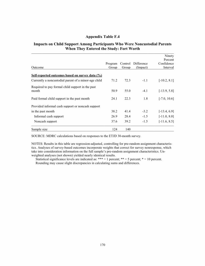
170
Appendix Table F.4
Self-reported outcomes based on survey data (%)
Impacts on Child Support Among Participants Who Were Noncustodial Parents When They Entered the Study: Fort Worth
Ninety
Percent Program Control Difference Confidence Outcome Group Group (Impact) Interval
Currently a noncustodial parent of a minor-age child 71.2 72.3 -1.1 [-10.2, 8.1]
Required to pay formal child support in the past month 50.9 55.0 -4.1 [-13.9, 5.8]
Paid formal child support in the past month 24.1 22.3 1.8 [-7.0, 10.6]
Provided informal cash support or noncash support in the past month 38.2 41.4 -3.2 [-13.4, 6.9]
Informal cash support 26.9 28.4 -1.5 [-11.0, 8.0] Noncash support 37.6 39.2 -1.5 [-11.6, 8.5]
Sample size 124 140
SOURCE: MDRC calculations based on responses to the ETJD 30-month survey.
NOTES: Results in this table are regression-adjusted, controlling for pre-random assignment characteris-tics. Analyses of survey-based outcomes incorporate weights that correct for survey nonresponse, which take into consideration information on the full sample’s pre-random assignment characteristics. Un-weighted analyses (not shown) yielded nearly identical results. Statistical significance levels are indicated as: *** = 1 percent; ** = 5 percent; * = 10 percent. Rounding may cause slight discrepancies in calculating sums and differences.
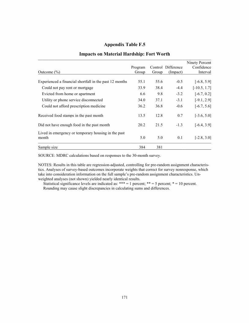
171
Appendix Table F.5
Impacts on Material Hardship: Fort Worth
Ninety Percent Program Control Difference Confidence Outcome (%) Group Group (Impact) Interval
Experienced a financial shortfall in the past 12 months 55.1 55.6 -0.5 [-6.8, 5.9] Could not pay rent or mortgage 33.9 38.4 -4.4 [-10.5, 1.7] Evicted from home or apartment 6.6 9.8 -3.2 [-6.7, 0.2] Utility or phone service disconnected 34.0 37.1 -3.1 [-9.1, 2.9] Could not afford prescription medicine 36.2 36.8 -0.6 [-6.7, 5.6]
Received food stamps in the past month 13.5 12.8 0.7 [-3.6, 5.0]
Did not have enough food in the past month 20.2 21.5 -1.3 [-6.4, 3.9]
Lived in emergency or temporary housing in the past month 5.0 5.0 0.1 [-2.8, 3.0]
Sample size 384 381
SOURCE: MDRC calculations based on responses to the 30-month survey.
NOTES: Results in this table are regression-adjusted, controlling for pre-random assignment characteris-tics. Analyses of survey-based outcomes incorporate weights that correct for survey nonresponse, which take into consideration information on the full sample’s pre-random assignment characteristics. Un-weighted analyses (not shown) yielded nearly identical results. Statistical significance levels are indicated as: *** = 1 percent; ** = 5 percent; * = 10 percent. Rounding may cause slight discrepancies in calculating sums and differences.
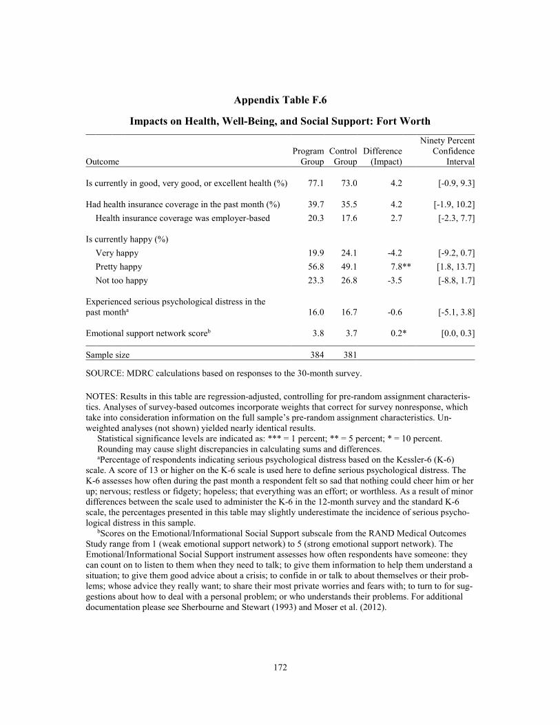
172
Appendix Table F.6
Impacts on Health, Well-Being, and Social Support: Fort Worth
Ninety Percent Program Control Difference Confidence Outcome Group Group (Impact) Interval
Is currently in good, very good, or excellent health (%) 77.1 73.0 4.2 [-0.9, 9.3]
Had health insurance coverage in the past month (%) 39.7 35.5 4.2 [-1.9, 10.2] Health insurance coverage was employer-based 20.3 17.6 2.7 [-2.3, 7.7]
Is currently happy (%) Very happy 19.9 24.1 -4.2 [-9.2, 0.7] Pretty happy 56.8 49.1 7.8 ** [1.8, 13.7] Not too happy 23.3 26.8 -3.5 [-8.8, 1.7]
Experienced serious psychological distress in the past montha 16.0 16.7 -0.6 [-5.1, 3.8]
Emotional support network scoreb 3.8 3.7 0.2 * [0.0, 0.3]
Sample size 384 381
SOURCE: MDRC calculations based on responses to the 30-month survey.
NOTES: Results in this table are regression-adjusted, controlling for pre-random assignment characteris-tics. Analyses of survey-based outcomes incorporate weights that correct for survey nonresponse, which take into consideration information on the full sample’s pre-random assignment characteristics. Un-weighted analyses (not shown) yielded nearly identical results. Statistical significance levels are indicated as: *** = 1 percent; ** = 5 percent; * = 10 percent. Rounding may cause slight discrepancies in calculating sums and differences. aPercentage of respondents indicating serious psychological distress based on the Kessler-6 (K-6) scale. A score of 13 or higher on the K-6 scale is used here to define serious psychological distress. The K-6 assesses how often during the past month a respondent felt so sad that nothing could cheer him or her up; nervous; restless or fidgety; hopeless; that everything was an effort; or worthless. As a result of minor differences between the scale used to administer the K-6 in the 12-month survey and the standard K-6 scale, the percentages presented in this table may slightly underestimate the incidence of serious psycho-logical distress in this sample. bScores on the Emotional/Informational Social Support subscale from the RAND Medical Outcomes Study range from 1 (weak emotional support network) to 5 (strong emotional support network). The Emotional/Informational Social Support instrument assesses how often respondents have someone: they can count on to listen to them when they need to talk; to give them information to help them understand a situation; to give them good advice about a crisis; to confide in or talk to about themselves or their prob-lems; whose advice they really want; to share their most private worries and fears with; to turn to for sug-gestions about how to deal with a personal problem; or who understands their problems. For additional documentation please see Sherbourne and Stewart (1993) and Moser et al. (2012).
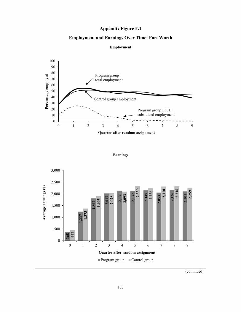
173
(continued)
Appendix Figure F.1
Employment and Earnings Over Time: Fort Worth
Employment
Earnings
0102030405060708090
100
0 1 2 3 4 5 6 7 8 9
Perc
enta
ge e
mpl
oyed
Quarter after random assignment
Program group total employment
Control group employment
368
1,23
7
1,80
7 2,01
7
2,13
1
2,13
2
2,14
9
2,05
3
2,16
2
2,10
1
447
1,37
3
1,90
5
2,02
8
2,09
3 2,33
0
2,23
6
2,31
0
2,31
8
2,25
9
0
500
1,000
1,500
2,000
2,500
3,000
0 1 2 3 4 5 6 7 8 9
Ave
rage
ear
ning
s ($)
Quarter after random assignment
Program group Control groupControl group
Program group ETJDsubsidized employment

174
Appendix Figure F.1 (continued)
SOURCES: MDRC calculations based on quarterly wage data from the National Directory of New Hiresand program payroll records.
NOTES: Results in this figure are regression-adjusted, controlling for pre-random assignment characteristics.
Statistical significance levels are indicated as: *** = 1 percent; ** = 5 percent; * = 10 percent.Employment rates and earnings in the quarter of random assignment through Quarter 5 after random
assignment include both ETJD subsidized jobs and jobs covered by unemployment insurance and reported to the National Directory of New Hires. Employment rates and earnings in Quarters 6 through 9 after random assignment include only jobs covered by unemployment insurance and reported to the National Directory of New Hires.
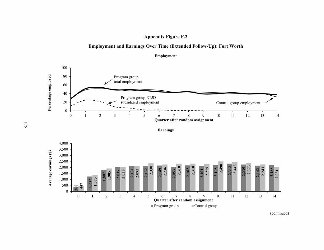
175
(continued)
Appendix Figure F.2
Employment and Earnings Over Time (Extended Follow-Up): Fort Worth
Employment
Earnings
0
20
40
60
80
100
0 1 2 3 4 5 6 7 8 9 10 11 12 13 14
Perc
enta
ge e
mpl
oyed
Quarter after random assignment
Program group total employment
Control group employment
368 1,23
7 1,80
7
2,01
7
2,13
1
2,13
2
2,14
9
2,05
3
2,16
2
2,10
1
2,19
8
2,31
2
2,23
5
2,14
2
2,18
8
447 1,37
3 1,90
5
2,02
8
2,09
3
2,33
0
2,23
6
2,31
0
2,31
8
2,25
9
2,49
0
2,44
3
2,37
3
2,24
3
2,03
1
0500
1,0001,5002,0002,5003,0003,5004,000
0 1 2 3 4 5 6 7 8 9 10 11 12 13 14
Ave
rage
ear
ning
s ($)
Quarter after random assignmentProgram group Control Group
Program group ETJDsubsidized employment
Control group

176
Appendix Figure F.2 (continued) SOURCES: MDRC calculations based on quarterly wage data from the National Directory of New Hires and program payroll records. NOTES: Results in this figure are regression-adjusted, controlling for pre-random assignment characteristics. Statistical significance levels are indicated as: *** = 1 percent; ** = 5 percent; * = 10 percent. Employment rates and earnings in the quarter of random assignment through Quarter 5 after random assignment include both ETJD subsidized jobs and jobs covered by unemployment insurance and re-ported to the National Directory of New Hires. Employment rates and earnings in Quarters 6 through 14 after random assignment include only jobs covered by unemployment insurance and reported to the Na-tional Directory of New Hires.

Appendix G
Supplementary Tables and Figures for Indianapolis

THIS PAGE INTENTIONALLY LEFT BLANK
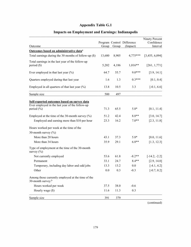
179
Appendix Table G.1
a
(continued)
Impacts on Employment and Earnings: Indianapolis
Outcome
Program Group
Control Group
Difference (Impact)
Ninety Percent Confidence
Interval Outcomes based on administrative data Total earnings during the 30 months of follow-up ($) 13,680 8,905 4,775 *** [3,455, 6,094]
Total earnings in the last year of the follow-up period ($) 5,202 4,186 1,016 ** [261, 1,771]
Ever employed in that last year (%) 64.7 55.7 9.0 *** [3.9, 14.1]
Quarters employed during that last year 1.6 1.3 0.3 *** [0.1, 0.4]
Employed in all quarters of that last year (%) 13.8 10.5 3.3 [-0.1, 6.6]
Sample size 500 497
Self-reported outcomes based on survey data Ever employed in the last year of the follow-up period (%) 71.3 65.5 5.8 * [0.1, 11.4]
Employed at the time of the 30-month survey (%) 51.2 42.4 8.8 ** [3.0, 14.7] Employed and earning more than $10 per hour 23.3 16.2 7.0 ** [2.3, 11.8]
Hours worked per week at the time of the 30-month survey (%)
More than 20 hours 43.1 37.3 5.8 * [0.0, 11.6] More than 34 hours 35.9 29.1 6.8 ** [1.3, 12.3]
Type of employment at the time of the 30-month survey (%)
Not currently employed 53.6 61.8 -8.2 ** [-14.2, -2.2] Permanent 33.1 24.7 8.4 ** [2.9, 14.0] Temporary, including day labor and odd jobs 13.3 13.2 0.0 [-4.1, 4.2] Other 0.0 0.3 -0.3 [-0.7, 0.2]
Among those currently employed at the time of the 30-month survey:b
Hours worked per week 37.5 38.0 -0.6 Hourly wage ($) 11.6 11.3 0.3
Sample size 391 379

180
Appendix Table G.1 (continued) SOURCES: MDRC calculations based on quarterly wage data from the National Directory of New Hires and responses to the ETJD 30-month survey. NOTES: Results in this table are regression-adjusted, controlling for pre-random assignment characteris-tics. Analyses of survey-based outcomes incorporate weights that correct for survey nonresponse, which take into consideration information on the full sample’s pre-random assignment characteristics. Un-weighted analyses (not shown) yielded nearly identical results. Statistical significance levels are indicated as: *** = 1 percent; ** = 5 percent; * = 10 percent. Rounding may cause slight discrepancies in calculating sums and differences. aEmployment rates and earnings include only jobs covered by unemployment insurance and reported to the National Directory of New Hires. bThese measures are calculated among those employed at the time of the survey; they are therefore considered nonexperimental and are not tested for statistical significance.

181
Appendix Table G.2
Impacts on Criminal Justice Outcomes: Indianapolis
Outcome Program
Group Control
Group Difference
(Impact)
Ninety Percent Confidence
Interval Outcomes based on administrative data Arrested, convicted, or admitted to jail or prison (%) 67.4 73.6 -6.2 ** [-10.7, -1.7]
Arrested (%) 46.4 51.0 -4.6 [-10.3, 1.1]
Convicted of a crime (%) 36.2 40.4 -4.2 [-9.8, 1.4] Convicted of a felony 20.3 25.2 -4.9 [-9.8, 0.1] Convicted of a misdemeanor 18.4 18.5 -0.1 [-4.7, 4.5]
Convicted of a violent crime (%) 7.5 6.7 0.8 [-2.3, 3.9]
Incarcerated (%) 66.1 72.5 -6.4 ** [-11.1, -1.7] Incarcerated in jail 64.3 68.8 -4.5 [-9.4, 0.3] Incarcerated in prison 31.3 39.9 -8.6 *** [-13.5, -3.8]
Prison admission reason (%)
Admitted to prison for a new crime 7.8 10.3 -2.5 [-5.5, 0.4] Admitted to prison for a parole or probation violation 24.7 30.3 -5.6 ** [-10.1, -1.0]
Total days incarcerated 161 209 -48 *** [-75, -21] Jail 72 86 -14 [-28, 0] Prison 90 121 -31 *** [-49, -12]
Sample size 491 491
SOURCE: MDRC calculations based on criminal justice data.
NOTES: Results in this table are regression-adjusted, controlling for pre-random assignment characteristics. Statistical significance levels are indicated as: *** = 1 percent; ** = 5 percent; * = 10 percent. Rounding may cause slight discrepancies in calculating sums and differences.
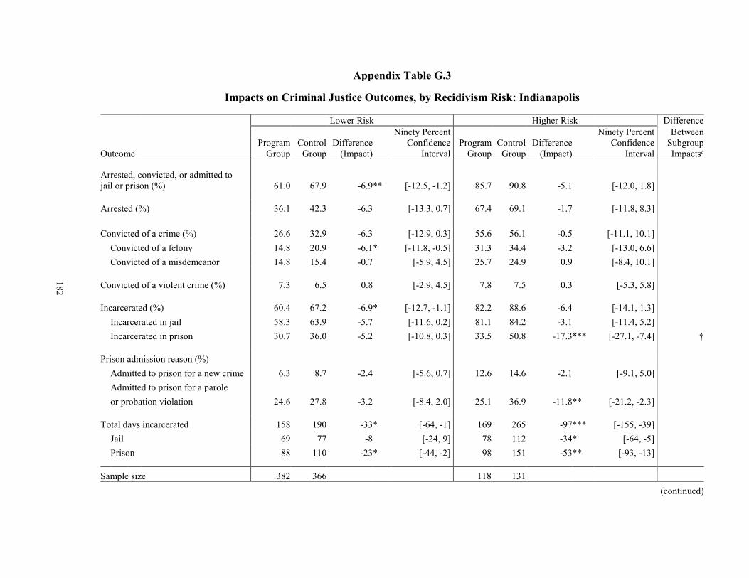
(continued)
Appendix Table G.3
Impacts on Criminal Justice Outcomes, by Recidivism Risk: Indianapolis
Lower Risk Higher Risk Difference Ninety Percent Ninety Percent Between Program Control Difference Confidence Program Control Difference Confidence Subgroup
Outcome Group Group (Impact) Interval Group Group (Impact) Interval Impactsa
Arrested, convicted, or admitted to jail or prison (%) 61.0 67.9 -6.9 ** [-12.5, -1.2] 85.7 90.8 -5.1 [-12.0, 1.8]
Arrested (%) 36.1 42.3 -6.3 [-13.3, 0.7] 67.4 69.1 -1.7 [-11.8, 8.3]
Convicted of a crime (%) 26.6 32.9 -6.3 [-12.9, 0.3] 55.6 56.1 -0.5 [-11.1, 10.1] Convicted of a felony 14.8 20.9 -6.1 * [-11.8, -0.5] 31.3 34.4 -3.2 [-13.0, 6.6] Convicted of a misdemeanor 14.8 15.4 -0.7 [-5.9, 4.5] 25.7 24.9 0.9 [-8.4, 10.1]
Convicted of a violent crime (%) 7.3 6.5 0.8 [-2.9, 4.5] 7.8 7.5 0.3 [-5.3, 5.8]
Incarcerated (%) 60.4 67.2 -6.9 * [-12.7, -1.1] 82.2 88.6 -6.4 [-14.1, 1.3] Incarcerated in jail 58.3 63.9 -5.7 [-11.6, 0.2] 81.1 84.2 -3.1 [-11.4, 5.2] Incarcerated in prison 30.7 36.0 -5.2 [-10.8, 0.3] 33.5 50.8 -17.3 *** [-27.1, -7.4] †
Prison admission reason (%) Admitted to prison for a new crime 6.3 8.7 -2.4 [-5.6, 0.7] 12.6 14.6 -2.1 [-9.1, 5.0] Admitted to prison for a parole or probation violation 24.6 27.8 -3.2 [-8.4, 2.0] 25.1 36.9 -11.8 ** [-21.2, -2.3]
Total days incarcerated 158 190 -33 * [-64, -1] 169 265 -97 *** [-155, -39] Jail 69 77 -8 [-24, 9] 78 112 -34 * [-64, -5] Prison 88 110 -23 * [-44, -2] 98 151 -53 ** [-93, -13]
Sample size 382 366 118 131
182

183
Appendix Table G.3 (continued) SOURCE: MDRC calculations based on criminal justice records. NOTES: Results in this table are regression-adjusted, controlling for pre-random assignment characteristics. Statistical significance levels are indicated as: *** = 1 percent; ** = 5 percent; * = 10 percent. Rounding may cause slight discrepancies in calculating sums and differences. See Appendix L for details on how risk of recidivism was defined. aWhen comparing impacts between two subgroups, an H-statistic is generated. The H-statistic is used to assess whether the difference in impacts between the subgroups is statistically significant. Statistically sig-nificant differences between subgroups are indicated as: ††† = 1 percent; †† = 5 percent; † = 10 percent.
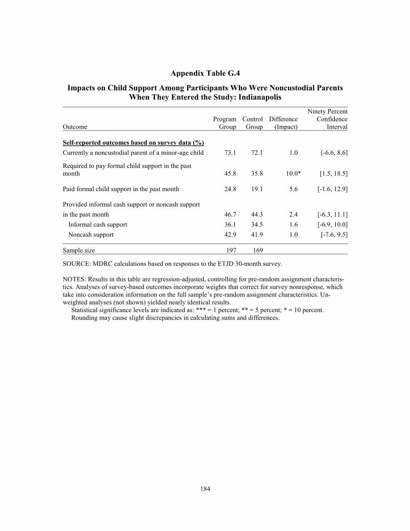
184
Appendix Table G.4
Impacts on Child Support Among Participants Who Were Noncustodial Parents When They Entered the Study: Indianapolis
Ninety Percent Program Control Difference Confidence Outcome Group Group (Impact) Interval
Self-reported outcomes based on survey data (%) Currently a noncustodial parent of a minor-age child 73.1 72.1 1.0 [-6.6, 8.6]
Required to pay formal child support in the past month 45.8 35.8 10.0 * [1.5, 18.5]
Paid formal child support in the past month 24.8 19.1 5.6 [-1.6, 12.9]
Provided informal cash support or noncash support in the past month 46.7 44.3 2.4 [-6.3, 11.1]
Informal cash support 36.1 34.5 1.6 [-6.9, 10.0] Noncash support 42.9 41.9 1.0 [-7.6, 9.5]
Sample size 197 169
SOURCE: MDRC calculations based on responses to the ETJD 30-month survey.
NOTES: Results in this table are regression-adjusted, controlling for pre-random assignment characteris-tics. Analyses of survey-based outcomes incorporate weights that correct for survey nonresponse, which take into consideration information on the full sample’s pre-random assignment characteristics. Un-weighted analyses (not shown) yielded nearly identical results. Statistical significance levels are indicated as: *** = 1 percent; ** = 5 percent; * = 10 percent. Rounding may cause slight discrepancies in calculating sums and differences.
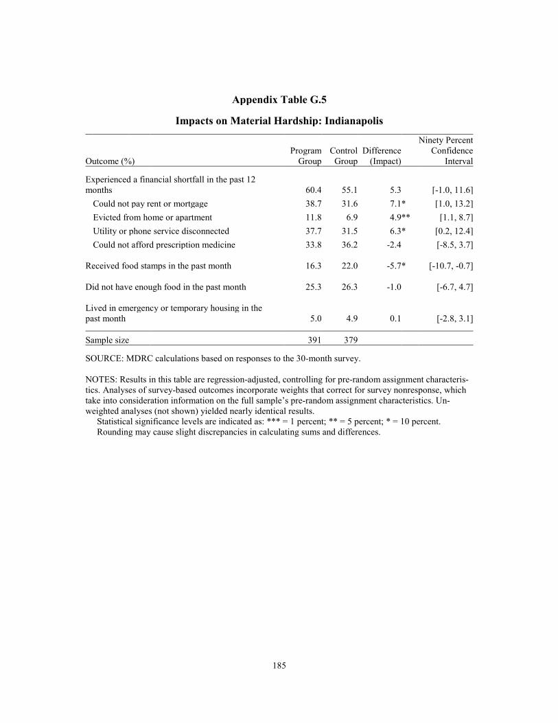
185
Appendix Table G.5
Impacts on Material Hardship: Indianapolis
Ninety Percent Program Control Difference Confidence Outcome (%) Group Group (Impact) Interval
Experienced a financial shortfall in the past 12 months 60.4 55.1 5.3 [-1.0, 11.6]
Could not pay rent or mortgage 38.7 31.6 7.1 * [1.0, 13.2] Evicted from home or apartment 11.8 6.9 4.9 ** [1.1, 8.7] Utility or phone service disconnected 37.7 31.5 6.3 * [0.2, 12.4] Could not afford prescription medicine 33.8 36.2 -2.4 [-8.5, 3.7]
Received food stamps in the past month 16.3 22.0 -5.7 * [-10.7, -0.7]
Did not have enough food in the past month 25.3 26.3 -1.0 [-6.7, 4.7]
Lived in emergency or temporary housing in the past month 5.0 4.9 0.1 [-2.8, 3.1]
Sample size 391 379
SOURCE: MDRC calculations based on responses to the 30-month survey.
NOTES: Results in this table are regression-adjusted, controlling for pre-random assignment characteris-tics. Analyses of survey-based outcomes incorporate weights that correct for survey nonresponse, which take into consideration information on the full sample’s pre-random assignment characteristics. Un-weighted analyses (not shown) yielded nearly identical results. Statistical significance levels are indicated as: *** = 1 percent; ** = 5 percent; * = 10 percent. Rounding may cause slight discrepancies in calculating sums and differences.
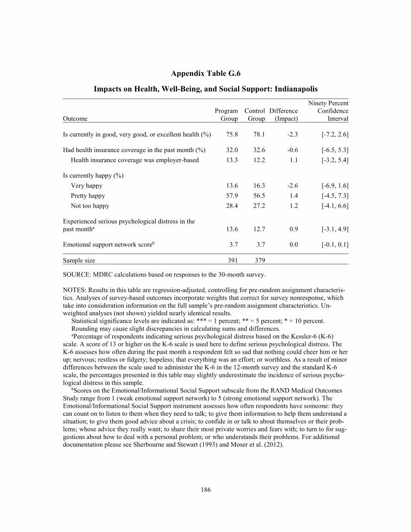
186
Appendix Table G.6
b
Impacts on Health, Well-Being, and Social Support: Indianapolis
Ninety Percent Program Control Difference Confidence Outcome Group Group (Impact) Interval
Is currently in good, very good, or excellent health (%) 75.8 78.1 -2.3 [-7.2, 2.6]
Had health insurance coverage in the past month (%) 32.0 32.6 -0.6 [-6.5, 5.3] Health insurance coverage was employer-based 13.3 12.2 1.1 [-3.2, 5.4]
Is currently happy (%) Very happy 13.6 16.3 -2.6 [-6.9, 1.6] Pretty happy 57.9 56.5 1.4 [-4.5, 7.3] Not too happy 28.4 27.2 1.2 [-4.1, 6.6]
Experienced serious psychological distress in the past montha 13.6 12.7 0.9 [-3.1, 4.9]
Emotional support network score 3.7 3.7 0.0 [-0.1, 0.1]
Sample size 391 379
SOURCE: MDRC calculations based on responses to the 30-month survey.
NOTES: Results in this table are regression-adjusted, controlling for pre-random assignment characteris-tics. Analyses of survey-based outcomes incorporate weights that correct for survey nonresponse, which take into consideration information on the full sample’s pre-random assignment characteristics. Un-weighted analyses (not shown) yielded nearly identical results. Statistical significance levels are indicated as: *** = 1 percent; ** = 5 percent; * = 10 percent. Rounding may cause slight discrepancies in calculating sums and differences. aPercentage of respondents indicating serious psychological distress based on the Kessler-6 (K-6) scale. A score of 13 or higher on the K-6 scale is used here to define serious psychological distress. The K-6 assesses how often during the past month a respondent felt so sad that nothing could cheer him or her up; nervous; restless or fidgety; hopeless; that everything was an effort; or worthless. As a result of minor differences between the scale used to administer the K-6 in the 12-month survey and the standard K-6 scale, the percentages presented in this table may slightly underestimate the incidence of serious psycho-logical distress in this sample. bScores on the Emotional/Informational Social Support subscale from the RAND Medical Outcomes Study range from 1 (weak emotional support network) to 5 (strong emotional support network). The Emotional/Informational Social Support instrument assesses how often respondents have someone: they can count on to listen to them when they need to talk; to give them information to help them understand a situation; to give them good advice about a crisis; to confide in or talk to about themselves or their prob-lems; whose advice they really want; to share their most private worries and fears with; to turn to for sug-gestions about how to deal with a personal problem; or who understands their problems. For additional documentation please see Sherbourne and Stewart (1993) and Moser et al. (2012).
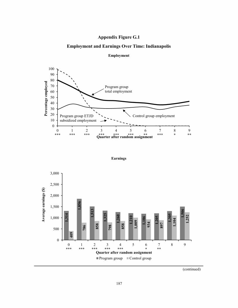
187
(continued)
Appendix Figure G.1
Employment and Earnings Over Time: Indianapolis
Employment
Earnings
0102030405060708090
100
0***
1***
2***
3***
4***
5***
6**
7***
8*
9**
Perc
enta
ge e
mpl
oyed
Quarter after random assignment
Program group total employment
Control group employment
1,31
4
1,85
6
1,51
3
1,32
5
1,26
0
1,21
0
1,18
6
1,20
5
1,30
5 1,50
6
409
786 858
798
858
1,00
9
934
897 1,10
4
1,25
2
0
500
1,000
1,500
2,000
2,500
3,000
0***
1***
2***
3***
4***
5 6*
7**
8 9
Ave
rage
ear
ning
s ($)
Quarter after random assignmentProgram group Control group
Program group ETJDsubsidized employment

188
Appendix Figure G.1 (continued)
SOURCES: MDRC calculations based on quarterly wage data from the National Directory of New Hiresand program payroll records.
NOTES: Results in this figure are regression-adjusted, controlling for pre-random assignment characteristics.
Statistical significance levels are indicated as: *** = 1 percent; ** = 5 percent; * = 10 percent.Employment rates and earnings in the quarter of random assignment through Quarter 5 after random
assignment include both ETJD subsidized jobs and jobs covered by unemployment insurance and reported to the National Directory of New Hires. Employment rates and earnings in Quarters 6 through 9 after random assignment include only jobs covered by unemployment insurance and reported to the National Directory of New Hires.
Although the Indianapolis ETJD program reported ETJD subsidized employment and earnings to the unemployment insurance system, ETJD subsidized employment rates among program group members based on payroll records appeared higher than total employment reported in unemployment insurance wage records during the quarter of random assignment. It is possible that timing differences in reporting and payroll periods contributed to this discrepancy.
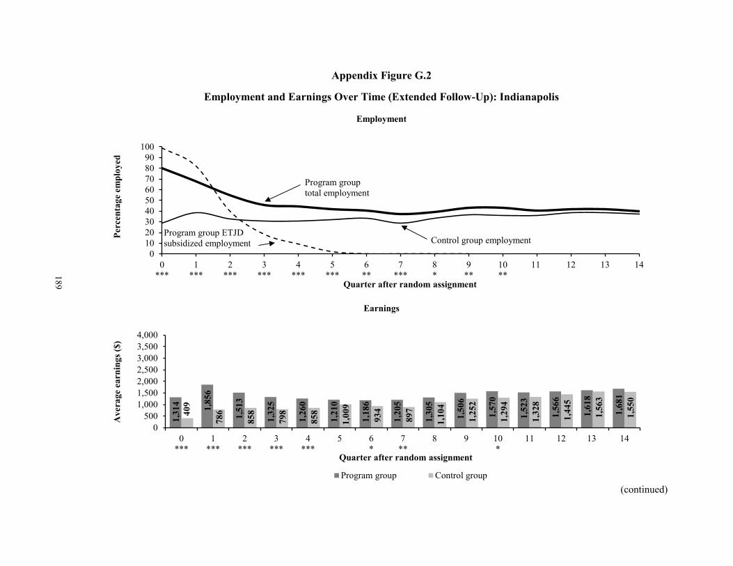
(continued)
Appendix Figure G.2
Employment and Earnings Over Time (Extended Follow-Up): Indianapolis
Employment
Earnings
0102030405060708090
100
0***
1***
2***
3***
4***
5***
6**
7***
8*
9**
10**
11 12 13 14
Perc
enta
ge e
mpl
oyed
Quarter after random assignment
Program group total employment
Control group employment
1,31
4 1,85
6
1,51
3
1,32
5
1,26
0
1,21
0
1,18
6
1,20
5
1,30
5
1,50
6
1,57
0
1,52
3
1,56
6
1,61
8
1,68
1
409
786
858
798
858
1,00
9
934
897
1,10
4
1,25
2
1,29
4
1,32
8
1,44
5
1,56
3
1,55
0
0500
1,0001,5002,0002,5003,0003,5004,000
0***
1***
2***
3***
4***
5 6*
7**
8 9 10*
11 12 13 14
Ave
rage
ear
ning
s ($)
Quarter after random assignment
Program group Control group
Program group ETJDsubsidized employment
189
190
Appendix Figure G.2 (continued) SOURCES: MDRC calculations based on quarterly wage data from the National Directory of New Hires and program payroll records. NOTES: Results in this figure are regression-adjusted, controlling for pre-random assignment characteristics. Statistical significance levels are indicated as: *** = 1 percent; ** = 5 percent; * = 10 percent. Employment rates and earnings in the quarter of random assignment through Quarter 5 after random assignment include both ETJD subsidized jobs and jobs covered by unemployment insurance and re-ported to the National Directory of New Hires. Employment rates and earnings in Quarters 6 through 14 after random assignment include only jobs covered by unemployment insurance and reported to the Na-tional Directory of New Hires. Although the Indianapolis ETJD program reported ETJD subsidized employment and earnings to the unemployment insurance system, ETJD subsidized employment rates among program group members based on payroll records appeared higher than total employment reported in unemployment insurance wage records during the quarter of random assignment. It is possible that timing differences in reporting and payroll periods contributed to this discrepancy.

Appendix H
Supplementary Tables and Figures for New York City

THIS PAGE INTENTIONALLY LEFT BLANK
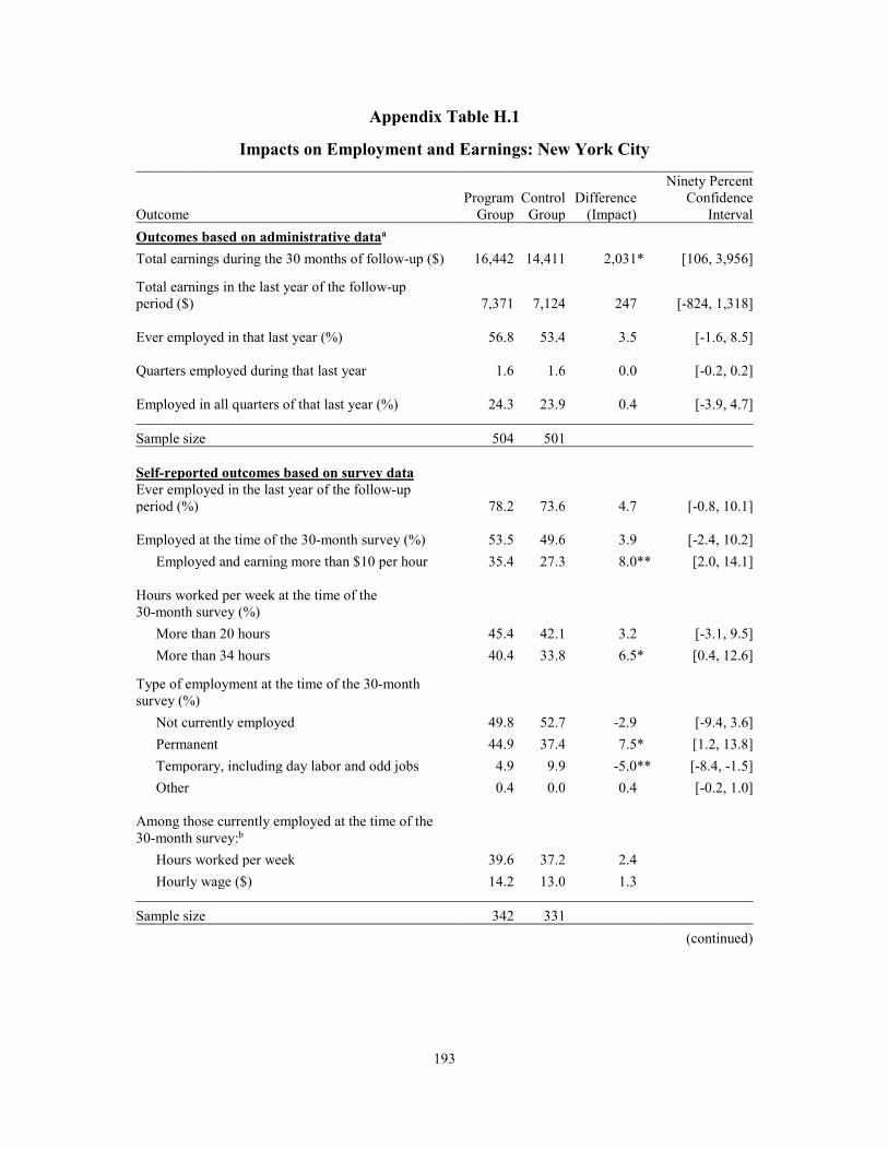
193
Appendix Table H.1
(continued)
Impacts on Employment and Earnings: New York City
Outcome
Program Group
Control Group
Difference (Impact)
Ninety Percent Confidence
Interval Outcomes based on administrative dataa Total earnings during the 30 months of follow-up ($) 16,442 14,411 2,031 * [106, 3,956]
Total earnings in the last year of the follow-up period ($) 7,371 7,124 247 [-824, 1,318]
Ever employed in that last year (%) 56.8 53.4 3.5 [-1.6, 8.5]
Quarters employed during that last year 1.6 1.6 0.0 [-0.2, 0.2]
Employed in all quarters of that last year (%) 24.3 23.9 0.4 [-3.9, 4.7]
Sample size 504 501
Self-reported outcomes based on survey data Ever employed in the last year of the follow-up period (%) 78.2 73.6 4.7 [-0.8, 10.1]
Employed at the time of the 30-month survey (%) 53.5 49.6 3.9 [-2.4, 10.2] Employed and earning more than $10 per hour 35.4 27.3 8.0 ** [2.0, 14.1]
Hours worked per week at the time of the 30-month survey (%)
More than 20 hours 45.4 42.1 3.2 [-3.1, 9.5] More than 34 hours 40.4 33.8 6.5 * [0.4, 12.6]
Type of employment at the time of the 30-month survey (%)
Not currently employed 49.8 52.7 -2.9 [-9.4, 3.6] Permanent 44.9 37.4 7.5 * [1.2, 13.8] Temporary, including day labor and odd jobs 4.9 9.9 -5.0 ** [-8.4, -1.5] Other 0.4 0.0 0.4 [-0.2, 1.0]
Among those currently employed at the time of the 30-month survey:b
Hours worked per week 39.6 37.2 2.4 Hourly wage ($) 14.2 13.0 1.3
Sample size 342 331

194
Appendix Table H.1 (continued) SOURCES: MDRC calculations based on quarterly wage data from the National Directory of New Hires and responses to the ETJD 30-month survey. NOTES: Results in this table are regression-adjusted, controlling for pre-random assignment characteris-tics. Analyses of survey-based outcomes incorporate weights that correct for survey nonresponse, which take into consideration information on the full sample’s pre-random assignment characteristics. Un-weighted analyses (not shown) yielded nearly identical results. Statistical significance levels are indicated as: *** = 1 percent; ** = 5 percent; * = 10 percent. Rounding may cause slight discrepancies in calculating sums and differences. aEmployment rates and earnings include only jobs covered by unemployment insurance and reported to the National Directory of New Hires. bThese measures are calculated among those employed at the time of the survey; they are therefore considered nonexperimental and are not tested for statistical significance.
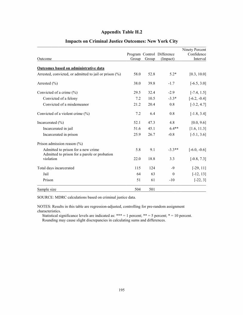
195
Appendix Table H.2
Impacts on Criminal Justice Outcomes: New York City
Outcome
Program Group
Control Group
Difference (Impact)
Ninety Percent Confidence
Interval
Outcomes based on administrative data Arrested, convicted, or admitted to jail or prison (%) 58.0 52.8 5.2 * [0.3, 10.0]
Arrested (%) 38.0 39.8 -1.7 [-6.5, 3.0]
Convicted of a crime (%) 29.5 32.4 -2.9 [-7.4, 1.5] Convicted of a felony 7.2 10.5 -3.3 * [-6.2, -0.4] Convicted of a misdemeanor 21.2 20.4 0.8 [-3.2, 4.7]
Convicted of a violent crime (%) 7.2 6.4 0.8 [-1.8, 3.4]
Incarcerated (%) 52.1 47.3 4.8 [0.0, 9.6] Incarcerated in jail 51.6 45.1 6.4 ** [1.6, 11.3] Incarcerated in prison 25.9 26.7 -0.8 [-5.1, 3.6]
Prison admission reason (%)
Admitted to prison for a new crime 5.8 9.1 -3.3 ** [-6.0, -0.6] Admitted to prison for a parole or probation violation 22.0 18.8 3.3 [-0.8, 7.3]
Total days incarcerated 115 124 -9 [-29, 11] Jail 64 63 0 [-12, 13] Prison 51 61 -10 [-22, 3]
Sample size 504 501
SOURCE: MDRC calculations based on criminal justice data.
NOTES: Results in this table are regression-adjusted, controlling for pre-random assignment characteristics. Statistical significance levels are indicated as: *** = 1 percent; ** = 5 percent; * = 10 percent.
Rounding may cause slight discrepancies in calculating sums and differences.
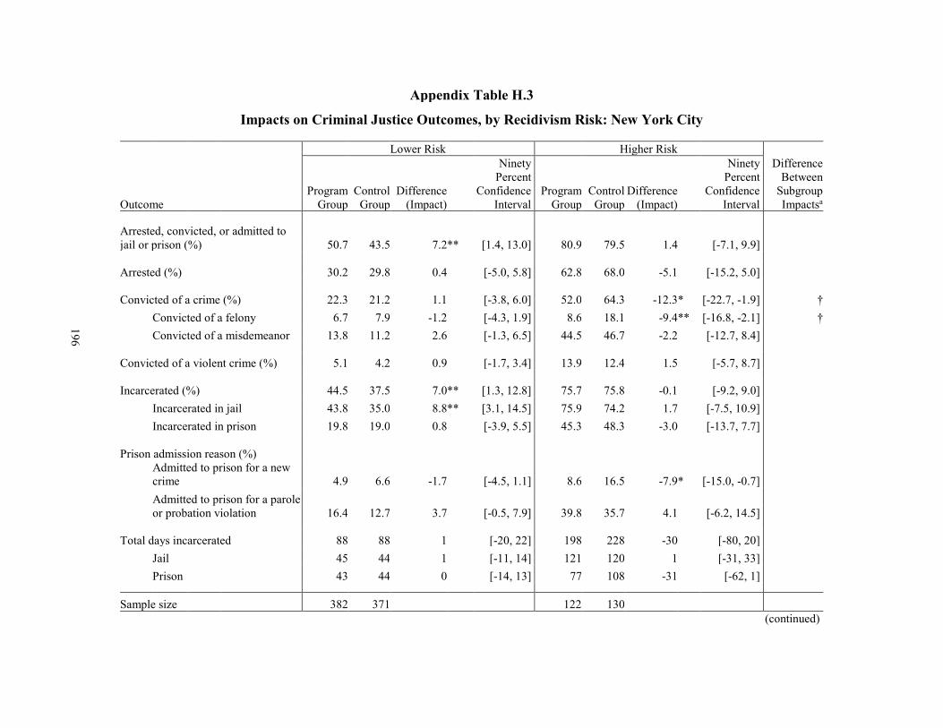
(continued)
Appendix Table H.3
Impacts on Criminal Justice Outcomes, by Recidivism Risk: New York City
Lower Risk Higher Risk Difference
Between Subgroup Impactsa Outcome
Program
Group Control
Group Difference
(Impact)
Ninety Percent
Confidence Interval
Program
Group Control
Group Difference
(Impact)
Ninety Percent
Confidence Interval
Arrested, convicted, or admitted to jail or prison (%) 50.7 43.5 7.2 ** [1.4, 13.0] 80.9 79.5 1.4 [-7.1, 9.9]
Arrested (%) 30.2 29.8 0.4 [-5.0, 5.8] 62.8 68.0 -5.1 [-15.2, 5.0]
Convicted of a crime (%) 22.3 21.2 1.1 [-3.8, 6.0] 52.0 64.3 -12.3 * [-22.7, -1.9] † Convicted of a felony 6.7 7.9 -1.2 [-4.3, 1.9] 8.6 18.1 -9.4 ** [-16.8, -2.1] † Convicted of a misdemeanor 13.8 11.2 2.6 [-1.3, 6.5] 44.5 46.7 -2.2 [-12.7, 8.4]
Convicted of a violent crime (%) 5.1 4.2 0.9 [-1.7, 3.4] 13.9 12.4 1.5 [-5.7, 8.7]
Incarcerated (%) 44.5 37.5 7.0 ** [1.3, 12.8] 75.7 75.8 -0.1 [-9.2, 9.0] Incarcerated in jail 43.8 35.0 8.8 ** [3.1, 14.5] 75.9 74.2 1.7 [-7.5, 10.9] Incarcerated in prison 19.8 19.0 0.8 [-3.9, 5.5] 45.3 48.3 -3.0 [-13.7, 7.7]
Prison admission reason (%) Admitted to prison for a new crime 4.9 6.6 -1.7 [-4.5, 1.1] 8.6 16.5 -7.9 * [-15.0, -0.7] Admitted to prison for a parole or probation violation
16.4 12.7 3.7 [-0.5, 7.9]
39.8 35.7 4.1 [-6.2, 14.5]
Total days incarcerated 88 88 1 [-20, 22] 198 228 -30 [-80, 20] Jail 45 44 1 [-11, 14] 121 120 1 [-31, 33] Prison 43 44 0 [-14, 13] 77 108 -31 [-62, 1]
Sample size 382 371 122 130
196

Appendix Table H.3 (continued) SOURCE: MDRC calculations based on criminal justice records. NOTES: Results in this table are regression-adjusted, controlling for pre-random assignment characteristics. Statistical significance levels are indicated as: *** = 1 percent; ** = 5 percent; * = 10 percent. Rounding may cause slight discrepancies in calculating sums and differences. See Appendix L for details on how risk of recidivism was defined. aWhen comparing impacts between two subgroups, an H-statistic is generated. The H-statistic is used to assess whether the difference in im-pacts between the subgroups is statistically significant. Statistically significant differences between subgroups are indicated as: ††† = 1 percent; †† = 5 percent; † = 10 percent.
197
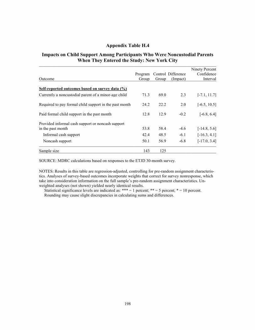
198
Appendix Table H.4
Impacts on Child Support Among Participants Who Were Noncustodial Parents When They Entered the Study: New York City
Ninety Percent Program Control Difference Confidence Outcome Group Group (Impact) Interval
Self-reported outcomes based on survey data (%) Currently a noncustodial parent of a minor-age child 71.3 69.0 2.3 [-7.1, 11.7]
Required to pay formal child support in the past month 24.2 22.2 2.0 [-6.5, 10.5]
Paid formal child support in the past month 12.8 12.9 -0.2 [-6.8, 6.4]
Provided informal cash support or noncash support in the past month 53.8 58.4 -4.6 [-14.8, 5.6]
Informal cash support 42.4 48.5 -6.1 [-16.3, 4.1] Noncash support 50.1 56.9 -6.8 [-17.0, 3.4]
Sample size 143 125
SOURCE: MDRC calculations based on responses to the ETJD 30-month survey.
NOTES: Results in this table are regression-adjusted, controlling for pre-random assignment characteris-tics. Analyses of survey-based outcomes incorporate weights that correct for survey nonresponse, which take into consideration information on the full sample’s pre-random assignment characteristics. Un-weighted analyses (not shown) yielded nearly identical results. Statistical significance levels are indicated as: *** = 1 percent; ** = 5 percent; * = 10 percent. Rounding may cause slight discrepancies in calculating sums and differences.

199
Appendix Table H.5
Impacts on Material Hardship: New York City
Ninety Percent Program Control Difference Confidence Outcome (%) Group Group (Impact) Interval
Experienced a financial shortfall in the past 12 months 47.2 44.5 2.7 [-3.8, 9.2] Could not pay rent or mortgage 29.8 31.0 -1.2 [-7.1, 4.8] Evicted from home or apartment 4.2 2.8 1.4 [-1.0, 3.8] Utility or phone service disconnected 26.1 29.0 -2.9 [-8.7, 3.0] Could not afford prescription medicine 18.4 16.6 1.8 [-3.1, 6.6]
Received food stamps in the past month 34.3 41.4 -7.0 * [-13.4, -0.7]
Did not have enough food in the past month 23.9 21.5 2.4 [-3.0, 7.8]
Lived in emergency or temporary housing in the past month 9.9 6.9 2.9 [-0.7, 6.5]
Sample size 342 331
SOURCE: MDRC calculations based on responses to the 30-month survey.
NOTES: Results in this table are regression-adjusted, controlling for pre-random assignment characteris-tics. Analyses of survey-based outcomes incorporate weights that correct for survey nonresponse, which take into consideration information on the full sample’s pre-random assignment characteristics. Un-weighted analyses (not shown) yielded nearly identical results. Statistical significance levels are indicated as: *** = 1 percent; ** = 5 percent; * = 10 percent. Rounding may cause slight discrepancies in calculating sums and differences.
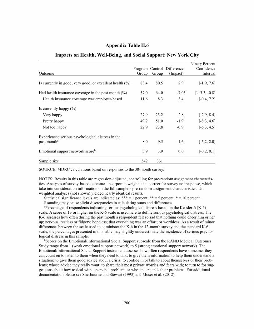
200
Appendix Table H.6
Impacts on Health, Well-Being, and Social Support: New York City
Ninety Percent Program Control Difference Confidence Outcome Group Group (Impact) Interval
Is currently in good, very good, or excellent health (%) 83.4 80.5 2.9 [-1.9, 7.6]
Had health insurance coverage in the past month (%) 57.0 64.0 -7.0 * [-13.3, -0.8] Health insurance coverage was employer-based 11.6 8.3 3.4 [-0.4, 7.2]
Is currently happy (%) Very happy 27.9 25.2 2.8 [-2.9, 8.4] Pretty happy 49.2 51.0 -1.9 [-8.3, 4.6] Not too happy 22.9 23.8 -0.9 [-6.3, 4.5]
Experienced serious psychological distress in the past montha 8.0 9.5 -1.6 [-5.2, 2.0]
Emotional support network scoreb 3.9 3.9 0.0 [-0.2, 0.1]
Sample size 342 331
SOURCE: MDRC calculations based on responses to the 30-month survey.
NOTES: Results in this table are regression-adjusted, controlling for pre-random assignment characteris-tics. Analyses of survey-based outcomes incorporate weights that correct for survey nonresponse, which take into consideration information on the full sample’s pre-random assignment characteristics. Un-weighted analyses (not shown) yielded nearly identical results. Statistical significance levels are indicated as: *** = 1 percent; ** = 5 percent; * = 10 percent. Rounding may cause slight discrepancies in calculating sums and differences. aPercentage of respondents indicating serious psychological distress based on the Kessler-6 (K-6) scale. A score of 13 or higher on the K-6 scale is used here to define serious psychological distress. The K-6 assesses how often during the past month a respondent felt so sad that nothing could cheer him or her up; nervous; restless or fidgety; hopeless; that everything was an effort; or worthless. As a result of minor differences between the scale used to administer the K-6 in the 12-month survey and the standard K-6 scale, the percentages presented in this table may slightly underestimate the incidence of serious psycho-logical distress in this sample. bScores on the Emotional/Informational Social Support subscale from the RAND Medical Outcomes Study range from 1 (weak emotional support network) to 5 (strong emotional support network). The Emotional/Informational Social Support instrument assesses how often respondents have someone: they can count on to listen to them when they need to talk; to give them information to help them understand a situation; to give them good advice about a crisis; to confide in or talk to about themselves or their prob-lems; whose advice they really want; to share their most private worries and fears with; to turn to for sug-gestions about how to deal with a personal problem; or who understands their problems. For additional documentation please see Sherbourne and Stewart (1993) and Moser et al. (2012).
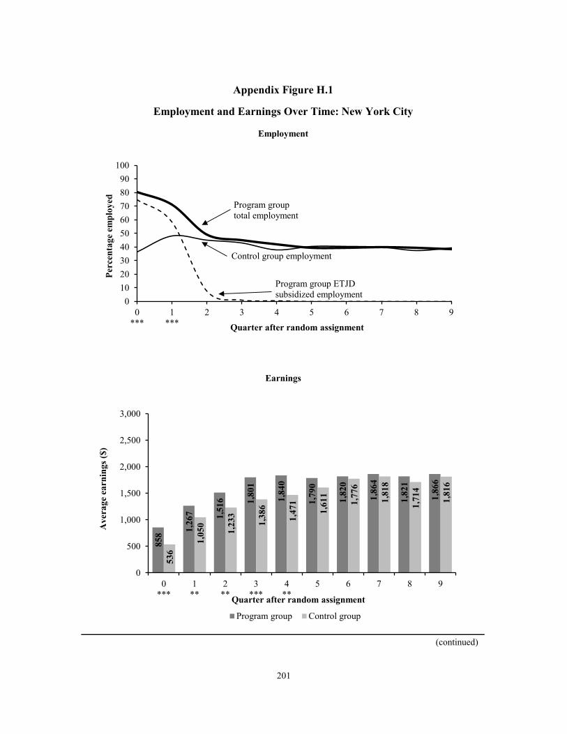
201
(continued)
Appendix Figure H.1
Employment and Earnings Over Time: New York City
Employment
Earnings
0102030405060708090
100
0***
1***
2 3 4 5 6 7 8 9
Perc
enta
ge e
mpl
oyed
Quarter after random assignment
Program group total employment
Control group employment
858 1,
267 1,51
6 1,80
1
1,84
0
1,79
0
1,82
0
1,86
4
1,82
1
1,86
6
536
1,05
0
1,23
3
1,38
6
1,47
1
1,61
1
1,77
6
1,81
8
1,71
4
1,81
6
0
500
1,000
1,500
2,000
2,500
3,000
0***
1**
2**
3***
4**
5 6 7 8 9
Ave
rage
ear
ning
s ($)
Quarter after random assignment
Program group Control group
Program group ETJDsubsidized employment

202
Appendix Figure H.1 (continued)
SOURCES: MDRC calculations based on quarterly wage data from the National Directory of New Hiresand program payroll records.
NOTES: Results in this figure are regression-adjusted, controlling for pre-random assignment characteristics.
Statistical significance levels are indicated as: *** = 1 percent; ** = 5 percent; * = 10 percent.Employment rates and earnings in the quarter of random assignment through Quarter 5 after random
assignment include both ETJD subsidized jobs and jobs covered by unemployment insurance and reported to the National Directory of New Hires. Employment rates and earnings in Quarters 6 through 9 after random assignment include only jobs covered by unemployment insurance and reported to the National Directory of New Hires.
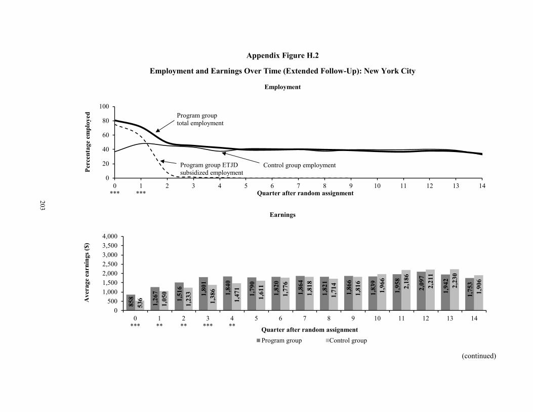
(continued)
Appendix Figure H.2
Employment and Earnings Over Time (Extended Follow-Up): New York City
Employment
Earnings
0
20
40
60
80
100
0***
1***
2 3 4 5 6 7 8 9 10 11 12 13 14
Perc
enta
ge e
mpl
oyed
Quarter after random assignment
Program group total employment
Control group employment
858
1,26
7
1,51
6
1,80
1
1,84
0
1,79
0
1,82
0
1,86
4
1,82
1
1,86
6
1,83
9
1,95
8
2,09
7
1,94
2
1,75
3
536
1,05
0
1,23
3
1,38
6
1,47
1
1,61
1
1,77
6
1,81
8
1,71
4
1,81
6
1,96
6
2,18
6
2,21
1
2,23
0
1,90
6
0500
1,0001,5002,0002,5003,0003,5004,000
0***
1**
2**
3***
4**
5 6 7 8 9 10 11 12 13 14
Ave
rage
ear
ning
s ($)
Quarter after random assignmentProgram group Control GroupControl group
Program group ETJDsubsidized employment
203

204
Appendix Figure H.2 (continued) SOURCES: MDRC calculations based on quarterly wage data from the National Directory of New Hires and program payroll records. NOTES: Results in this figure are regression-adjusted, controlling for pre-random assignment character-istics. Statistical significance levels are indicated as: *** = 1 percent; ** = 5 percent; * = 10 percent. Employment rates and earnings in the quarter of random assignment through Quarter 5 after random assignment include both ETJD subsidized jobs and jobs covered by unemployment insurance and re-ported to the National Directory of New Hires. Employment rates and earnings in Quarters 6 through 14 after random assignment include only jobs covered by unemployment insurance and reported to the Na-tional Directory of New Hires.

Appendix I
Baseline Characteristics of the Study Sample

THIS PAGE INTENTIONALLY LEFT BLANK

207
Appendix Table I.1
Marital status (%)
Characteristics and Employment Histories of Sample Members: Noncustodial Parent Sites
Program ControlCharacteristic Group Group
Male (%) 93.1 93.3
Age (%) 18-24 7.8 7.325-34 33.0 32.335-44 34.4 35.445 or older 24.9 25.0
Average age 37.6 37.6
Race/ethnicity (%) Black, non-Hispanic 81.5 83.3White, non-Hispanic 5.9 5.1Hispanic 7.8 7.9Asian, non-Hispanic 1.4 1.3Other/multiracial 3.3 2.4
Educational attainment (%) No high school diploma or equivalent 27.9 30.6High school diploma or equivalent 66.8 65.0Associate’s degree or equivalent 2.9 2.2Bachelor’s degree or higher 2.4 2.2
Never married 67.2 65.1Currently married 8.0 8.7Separated, widowed, or divorced 24.8 26.1
Veteran (%) 5.4 4.2 *
Has a disability (%) 5.9 4.9
Housing (%) Rents or owns 44.3 46.5Halfway house, transitional house, or residential treatment facility 3.6 3.8Homeless 7.3 8.5Staying in someone else’s apartment, room, or house 44.7 41.2
(continued)
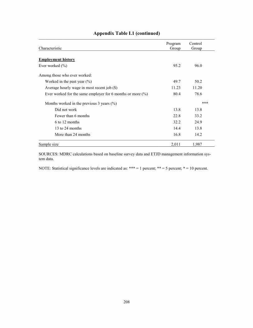
208
Appendix Table I.1 (continued)
Program Control Characteristic Group Group
Employment history Ever worked (%) 95.2 96.0
Among those who ever worked: Worked in the past year (%) 49.7 50.2Average hourly wage in most recent job ($) 11.23 11.20Ever worked for the same employer for 6 months or more (%) 80.4 78.6
Months worked in the previous 3 years (%) *** Did not work 13.8 13.8Fewer than 6 months 22.8 33.26 to 12 months 32.2 24.913 to 24 months 14.4 13.8More than 24 months 16.8 14.2
Sample size 2,011 1,987
SOURCES: MDRC calculations based on baseline survey data and ETJD management information sys-tem data.
NOTE: Statistical significance levels are indicated as: *** = 1 percent; ** = 5 percent; * = 10 percent.
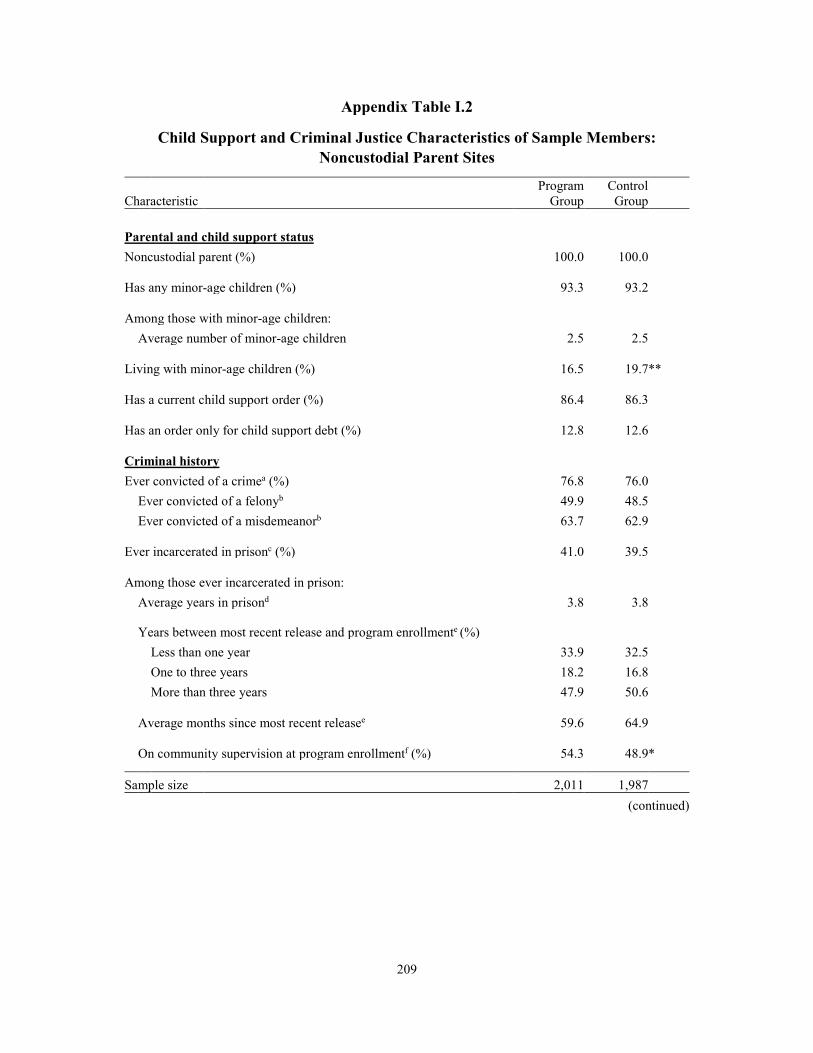
209
Appendix Table I.2
Criminal history
b
e
(continued)
Child Support and Criminal Justice Characteristics of Sample Members: Noncustodial Parent Sites
Program Control Characteristic Group Group
Parental and child support status Noncustodial parent (%) 100.0 100.0
Has any minor-age children (%) 93.3 93.2
Among those with minor-age children: Average number of minor-age children 2.5 2.5
Living with minor-age children (%) 16.5 19.7 **
Has a current child support order (%) 86.4 86.3
Has an order only for child support debt (%) 12.8 12.6
Ever convicted of a crimea (%) 76.8 76.0
Ever convicted of a felony 49.9 48.5 Ever convicted of a misdemeanorb 63.7 62.9
Ever incarcerated in prisonc (%) 41.0 39.5
Among those ever incarcerated in prison: Average years in prisond 3.8 3.8
Years between most recent release and program enrollmente (%) Less than one year 33.9 32.5 One to three years 18.2 16.8 More than three years 47.9 50.6
Average months since most recent release 59.6 64.9
On community supervision at program enrollmentf (%) 54.3 48.9 *
Sample size 2,011 1,987

210
Appendix Table I.2 (continued) SOURCES: MDRC calculations based on baseline survey data, ETJD management information system data, and criminal justice administrative records.
NOTES: Measures are self-reported unless otherwise noted. Statistical significance levels are indicated as: *** = 1 percent; ** = 5 percent; * = 10 percent. aIncludes convictions in the state in which the program operated as recorded in administrative records. Does not include federal convictions or convictions from other states. bAdministrative records from Wisconsin were not available on this subject. Therefore this measure re-flects data only from Atlanta, San Francisco, and Syracuse. cFor Atlanta, Milwaukee, and Syracuse, this measure includes participants’ reports of incarceration in state or federal prison and prison incarceration as recorded in administrative records from the state in which the program operated. For San Francisco, this measure only includes participants’ reports of incar-ceration. Administrative prison records from California were not available on this subject at the time of this report. dIncludes time spent in state prisons in the state in which the program operated, according to adminis-trative records. Does not include time spent in federal prisons or prisons in other states. Administrative prison records from California were not available on this subject at the time of this report, so this measure only reflects data from Atlanta, Milwaukee, and Syracuse. eMost recent release can be from prison or jail. fIncludes parole, probation, and other types of criminal justice or court supervision.
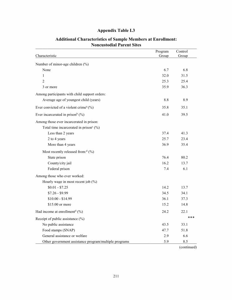
211
(continued)
Appendix Table I.3
Additional Characteristics of Sample Members at Enrollment: Noncustodial Parent Sites
Program Control Characteristic Group Group
Number of minor-age children (%)
None 6.7 6.8
1
32.0 31.5
2 25.3 25.4
3 or more 35.9 36.3
Among participants with child support orders:
Average age of youngest child (years) 8.8 8.9
Ever convicted of a violent crimea (%) 35.8 35.1
Ever incarcerated in prisonb (%) 41.0 39.5
Among those ever incarcerated in prison: Total time incarcerated in prisonc (%)
Less than 2 years 37.4 41.3
2 to 4 years 25.7 23.4
More than 4 years 36.9 35.4
Most recently released from:d (%)
State prison 76.4 80.2
County/city jail 16.2 13.7
Federal prison 7.4 6.1
Among those who ever worked: Hourly wage in most recent job (%)
$0.01 - $7.25 14.2 13.7
$7.26 - $9.99 34.5 34.1
$10.00 - $14.99 36.1 37.3
$15.00 or more 15.2 14.8
Had income at enrollmentd (%) 24.2 22.1 Receipt of public assistance (%) ***
No public assistance 43.5 33.1
Food stamps (SNAP) 47.7 51.8
General assistance or welfare 2.9 6.6
Other government assistance program/multiple programs 5.9 8.5
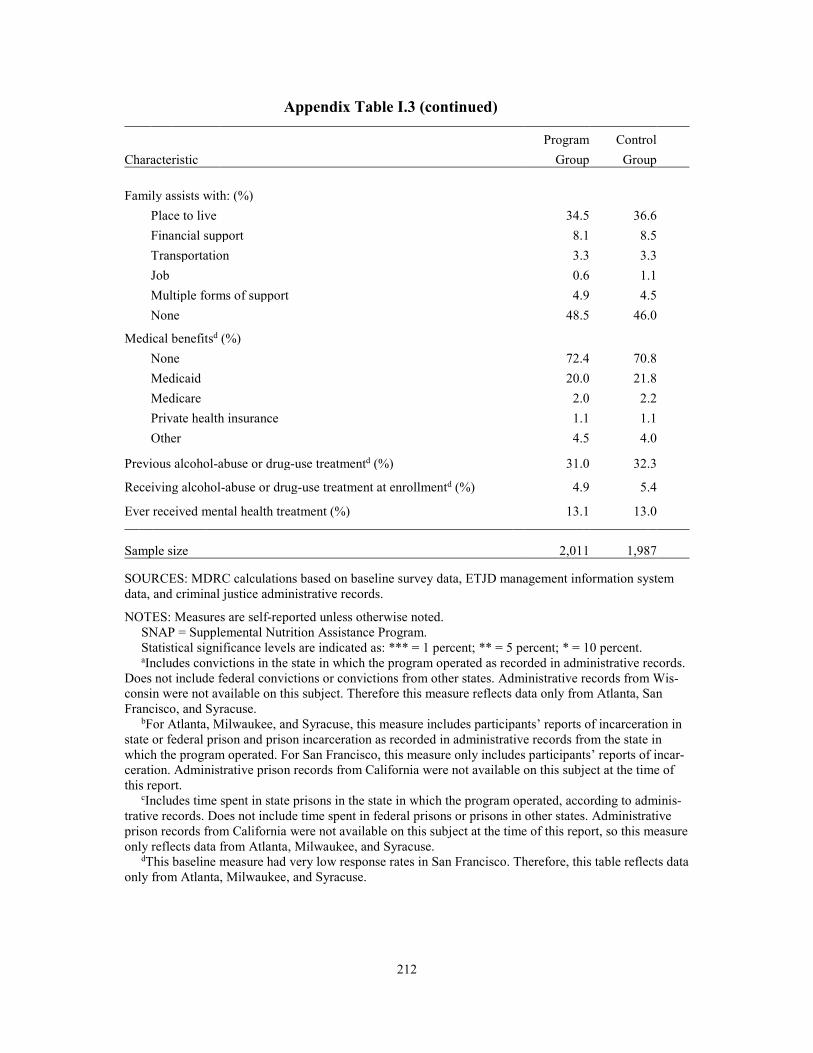
212
Appendix Table I.3 (continued)
Program Control Characteristic Group Group
Family assists with: (%) Place to live 34.5 36.6 Financial support 8.1 8.5 Transportation 3.3 3.3 Job 0.6 1.1 Multiple forms of support 4.9 4.5 None 48.5 46.0
Medical benefitsd (%) None 72.4 70.8 Medicaid 20.0 21.8 Medicare 2.0 2.2 Private health insurance 1.1 1.1 Other 4.5 4.0
Previous alcohol-abuse or drug-use treatmentd (%) 31.0 32.3 Receiving alcohol-abuse or drug-use treatment at enrollmentd (%) 4.9 5.4 Ever received mental health treatment (%) 13.1 13.0
Sample size 2,011 1,987
SOURCES: MDRC calculations based on baseline survey data, ETJD management information system data, and criminal justice administrative records.
NOTES: Measures are self-reported unless otherwise noted. SNAP = Supplemental Nutrition Assistance Program. Statistical significance levels are indicated as: *** = 1 percent; ** = 5 percent; * = 10 percent. aIncludes convictions in the state in which the program operated as recorded in administrative records. Does not include federal convictions or convictions from other states. Administrative records from Wis-consin were not available on this subject. Therefore this measure reflects data only from Atlanta, San Francisco, and Syracuse. bFor Atlanta, Milwaukee, and Syracuse, this measure includes participants’ reports of incarceration in state or federal prison and prison incarceration as recorded in administrative records from the state in which the program operated. For San Francisco, this measure only includes participants’ reports of incar-ceration. Administrative prison records from California were not available on this subject at the time of this report. cIncludes time spent in state prisons in the state in which the program operated, according to adminis-trative records. Does not include time spent in federal prisons or prisons in other states. Administrative prison records from California were not available on this subject at the time of this report, so this measure only reflects data from Atlanta, Milwaukee, and Syracuse. dThis baseline measure had very low response rates in San Francisco. Therefore, this table reflects data only from Atlanta, Milwaukee, and Syracuse.
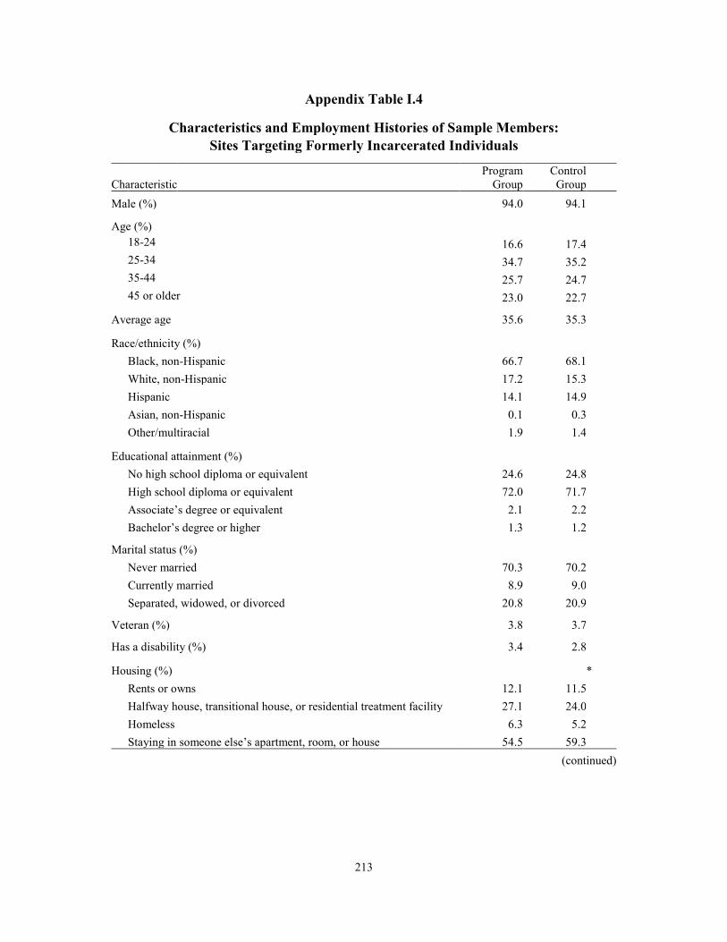
213
Appendix Table I.4
(continued)
Characteristics and Employment Histories of Sample Members: Sites Targeting Formerly Incarcerated Individuals
Program Control Characteristic Group Group Male (%) 94.0 94.1
Age (%) 18-24 16.6 17.4 25-34 34.7 35.2 35-44 25.7 24.7 45 or older 23.0 22.7
Average age 35.6 35.3
Race/ethnicity (%) Black, non-Hispanic 66.7 68.1 White, non-Hispanic 17.2 15.3 Hispanic 14.1 14.9 Asian, non-Hispanic 0.1 0.3 Other/multiracial 1.9 1.4
Educational attainment (%) No high school diploma or equivalent 24.6 24.8 High school diploma or equivalent 72.0 71.7 Associate’s degree or equivalent 2.1 2.2 Bachelor’s degree or higher 1.3 1.2
Marital status (%) Never married 70.3 70.2 Currently married 8.9 9.0 Separated, widowed, or divorced 20.8 20.9
Veteran (%) 3.8 3.7 Has a disability (%) 3.4 2.8
Housing (%) * Rents or owns 12.1 11.5 Halfway house, transitional house, or residential treatment facility 27.1 24.0 Homeless 6.3 5.2 Staying in someone else’s apartment, room, or house 54.5 59.3
214
Appendix Table I.4 (continued) Characteristic
Program Group
Control Group
Employment history Ever worked (%) 80.7 81.5
Among those who ever worked: Worked in the past year (%) 20.3 19.5 Average hourly wage in most recent job ($) 10.11 10.10 Ever worked for the same employer for 6 months or more (%) 74.0 71.8
Months worked in the previous 3 years (%) Did not work 46.0 47.2 Fewer than 6 months 31.1 29.9 6 to 12 months 13.8 12.1 13 to 24 months 6.3 7.1 More than 24 months 2.7 3.7
Sample size 1,508 1,494
SOURCES: MDRC calculations based on baseline survey data and ETJD management information sys-tem data.
NOTE: Statistical significance levels are indicated as: *** = 1 percent; ** = 5 percent; * = 10 percent.
215
Appendix Table I.5
Child Support and Criminal Justice Characteristics of Sample Members: Sites Targeting Formerly Incarcerated Individuals
Program Control Characteristic Group Group
Parental and child support status Noncustodial parent (%) 41.8 42.4 Has any minor-age children (%) 51.8 51.1 Among those with minor-age children:
Average number of minor-age children 2.1 2.1
Living with minor-age children (%) 14.2 13.7 Has a current child support order (%) 15.6 14.8 Has an order only for child support debt (%) 0.8 0.7 Criminal history Ever convicted of a crimea (%) 96.1 96.6
Ever convicted of a felony 90.5 91.5 Ever convicted of a misdemeanor 66.1 64.3
Ever incarcerated in prison (%) 100.0 100.0 Average years in jail and prisonb 4.7 4.9 Average months since most recent releasec 1.4 1.5 Status at program enrollment (%)
Parole 74.5 76.6 Probation 12.6 11.2 Other criminal justice/court supervision 10.4 8.8 None of the above 2.5 3.3
Sample size 1,508 1,494
SOURCES: MDRC calculations based on baseline survey data, ETJD management information system data, and criminal justice administrative records.
NOTES: Measures are self-reported unless otherwise noted. Statistical significance levels are indicated as: *** = 1 percent; ** = 5 percent; * = 10 percent. aIncludes convictions in the state in which the program operated as recorded in administrative records. Does not include federal convictions or convictions from other states. bIncludes time spent in state prisons and local jails in the state in which the program operated accord-ing to administrative records. Does not include time spent in federal prisons or prisons in other states. cMost recent release can be from prison or jail.
216
Appendix Table I.6
a
b
Additional Characteristics of Sample Members at Enrollment: Sites Targeting Formerly Incarcerated Individuals
Program Control Characteristic Group Group
Number of minor-age children (%) None 48.2 48.9 1
22.8 22.5 2 14.6 14.6 3 or more 14.3 14.1
Among participants with child support orders: Average age of youngest child (years) 9.6 9.6
Ever convicted of a violent crime (%) 49.2 49.6
Total time incarcerated in jail or prison (%) Less than two years 33.1 29.6 Two to four years 26.9 29.2 More than four years 39.9 41.2
Most recently released from (%) State prison 89.0 90.2 County/city jail 4.7 4.9 Federal prison 6.3 4.9
Among those who ever worked: Hourly wage in most recent job (%)
$0.01 - $7.25 22.2 23.6 $7.26 - $9.99 37.4 38.6 $10.00 - $14.99 30.1 26.4 $15.00 or more 10.4 11.4
Had income at enrollment (%) 4.0 3.7
Receipt of public assistance (%) No public assistance 69.5 67.5 Food stamps (SNAP) 21.9 25.3 General assistance or welfare 4.5 3.9 Other government assistance program/multiple programs 4.1 3.4 (continued)
217
Appendix Table I.6 (continued)
Program Control Characteristic Group Group Family assists with: (%)
Place to live 54.6 56.2 Financial support 7.6 8.1 Transportation 4.5 5.0 Job 0.5 0.4 Multiple forms of support 3.0 2.9 None 28.9 27.1
Medical benefits None 70.3 70.1 Medicaid 20.8 21.6 Medicare 0.3 0.1 Private health insurance 0.8 0.8 Other 7.9 7.4
Previous alcohol-abuse or drug-use treatment (%) 48.3 48.2
Receiving alcohol-abuse or drug-use treatment at enrollment (%) 24.7 25.9
Ever received mental health treatment (%) 11.1 7.5 ***
Sample size 1,508 1,494
SOURCES: MDRC calculations based on baseline survey data, ETJD management information system data, and criminal justice administrative records.
NOTES: Measures are self-reported unless otherwise noted. SNAP = Supplemental Nutrition Assistance Program. Statistical significance levels are indicated as: *** = 1 percent; ** = 5 percent; * = 10 percent. aIncludes convictions in the state in which the program operated as recorded in administrative rec-ords. Does not include federal convictions or convictions from other states. bIncludes time spent in state prisons and local jails in the state in which the program operated accord-ing to administrative records. Does not include time spent in federal prisons or prisons in other states.

THIS PAGE INTENTIONALLY LEFT BLANK

Appendix J
Selected Measures of Well-Being, by Site

THIS PAGE INTENTIONALLY LEFT BLANK
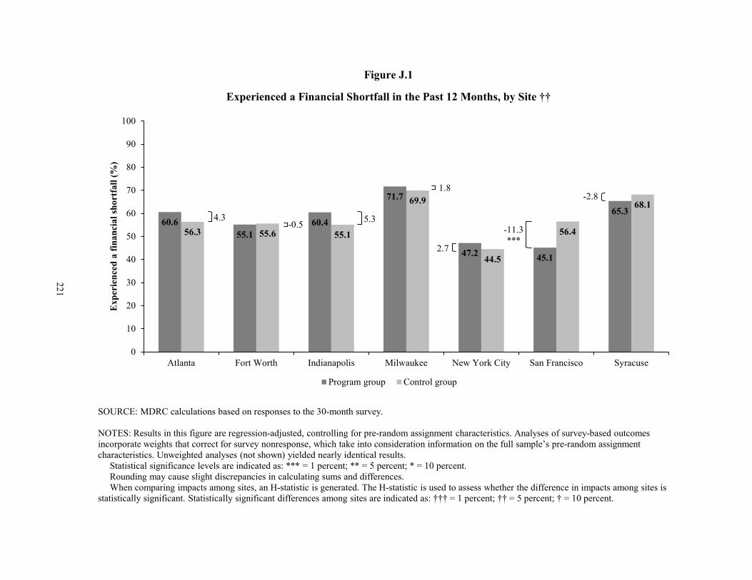
Figure J.1
Experienced a Financial Shortfall in the Past 12 Months, by Site ††
-0.5 -11.3***
-2.8
4.3 5.3
1.8
2.7
60.655.1
60.4
71.7
47.2 45.1
65.3
56.3 55.6 55.1
69.9
44.5
56.4
68.1
0
10
20
30
40
50
60
70
80
90
100
Atlanta Fort Worth Indianapolis Milwaukee New York City San Francisco Syracuse
Expe
rien
ced
a fin
anci
al sh
ortf
all (
%)
Program group Control group
221
SOURCE: MDRC calculations based on responses to the 30-month survey.
NOTES: Results in this figure are regression-adjusted, controlling for pre-random assignment characteristics. Analyses of survey-based outcomes incorporate weights that correct for survey nonresponse, which take into consideration information on the full sample’s pre-random assignment characteristics. Unweighted analyses (not shown) yielded nearly identical results.
Statistical significance levels are indicated as: *** = 1 percent; ** = 5 percent; * = 10 percent.Rounding may cause slight discrepancies in calculating sums and differences.When comparing impacts among sites, an H-statistic is generated. The H-statistic is used to assess whether the difference in impacts among sites is
statistically significant. Statistically significant differences among sites are indicated as: ††† = 1 percent; †† = 5 percent; † = 10 percent.
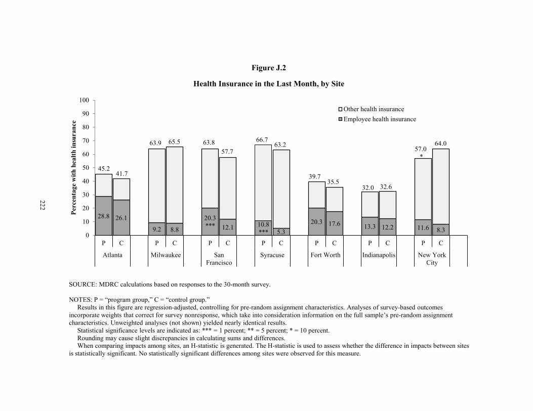
222
Figure J.2
Health Insurance in the Last Month, by Site
28.8 26.1
9.2 8.8
20.3*** 12.1 10.8
*** 5.320.3 17.6 13.3 12.2 11.6 8.3
0
10
20
30
40
50
60
70
80
90
100
P C P C P C P C P C P C P C
Atlanta Milwaukee SanFrancisco
Syracuse Fort Worth Indianapolis New YorkCity
Perc
enta
ge w
ith h
ealth
insu
ranc
e
Other health insuranceEmployee health insurance
45.241.7
63.9 65.5 63.857.7
66.763.2
39.735.5
57.0*
64.0
32.0 32.6
SOURCE: MDRC calculations based on responses to the 30-month survey.
NOTES: P = “program group,ˮ C = “control group.ˮ Results in this figure are regression-adjusted, controlling for pre-random assignment characteristics. Analyses of survey-based outcomes
incorporate weights that correct for survey nonresponse, which take into consideration information on the full sample’s pre-random assignment characteristics. Unweighted analyses (not shown) yielded nearly identical results.
Statistical significance levels are indicated as: *** = 1 percent; ** = 5 percent; * = 10 percent.Rounding may cause slight discrepancies in calculating sums and differences.When comparing impacts among sites, an H-statistic is generated. The H-statistic is used to assess whether the difference in impacts between sites
is statistically significant. No statistically significant differences among sites were observed for this measure.
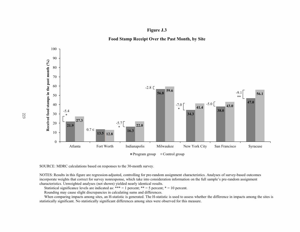
Figure J.3
Food Stamp Receipt Over the Past Month, by Site
-5.4*
-5.7*
-2.8
-7.0*
-5.0
-9.1**
0.721.9
13.516.3
56.8
34.338.0
47.0
27.3
12.8
22.0
59.6
41.4 43.0
56.1
0
10
20
30
40
50
60
70
80
90
100
Atlanta Fort Worth Indianapolis Milwaukee New York City San Francisco Syracuse
Rec
eive
d fo
od st
amps
in th
e pa
st m
onth
(%)
Program group Control group
223
SOURCE: MDRC calculations based on responses to the 30-month survey.
NOTES: Results in this figure are regression-adjusted, controlling for pre-random assignment characteristics. Analyses of survey-based outcomes incorporate weights that correct for survey nonresponse, which take into consideration information on the full sample’s pre-random assignment characteristics. Unweighted analyses (not shown) yielded nearly identical results.
Statistical significance levels are indicated as: *** = 1 percent; ** = 5 percent; * = 10 percent.Rounding may cause slight discrepancies in calculating sums and differences.When comparing impacts among sites, an H-statistic is generated. The H-statistic is used to assess whether the difference in impacts among the sites is
statistically significant. No statistically significant differences among sites were observed for this measure.

THIS PAGE INTENTIONALLY LEFT BLANK

Appendix K
Survey Response Bias Analysis

THIS PAGE INTENTIONALLY LEFT BLANK
227
This appendix assesses the reliability of the impact results captured by the Enhanced Transitional Jobs Demonstration (ETJD) 30-month survey for each of the seven program locations discussed in this report: Atlanta, Milwaukee, San Francisco, Syracuse, Fort Worth, Indianapolis, and New York. It also examines whether the program impacts for the survey respondents can be considered to represent the impacts for the full research sample. First, the appendix describes how the survey was administered, including survey response rates for the full research sample and the program and control groups in each city. Next, it examines the differences between survey respondents and nonrespondents, then compares the differences between the program and control groups among the survey respondents. Finally, it compares the administrative data outcomes of the re-spondent sample with those of the full research sample, both for the pooled research samples used throughout the report and within each city. The appendix concludes that there is no substantial concern about bias arising from survey nonresponse.
Survey Administration and Response Rates The ETJD 30-month survey was administered by Decision Information Resources in Atlanta and San Francisco and by Abt SRBI in Fort Worth, Indianapolis, Milwaukee, New York City, and Syracuse. Interviewers from the survey firms began interviewing sample members as early as 30 months after they enrolled into the study.1 For example, if a sample member were randomly as-signed into the study in January 2013, a survey firm would begin attempting to reach this sample member for the 30-month survey at the end of June 2015. Nearly all respondents (96 percent) were interviewed within the target window of 30 to 36 months after they enrolled in the study.2 Some respondents were interviewed while they were incarcerated. Abt SRBI succeeded in gain-ing access to prisons and jails where ETJD sample members from five cities were incarcerated: Fort Worth (62 facilities), Indianapolis (12 facilities), Milwaukee (9 facilities), New York (1 fa-cility: Rikers Island), and Syracuse (1 facility: Onandaga County Jail). Decision Information Re-sources did not gain access to prisons and jails.
Table K.1 shows the response rate for each city and the percentage of responses that were “on time” (defined as completing the survey interview between 27 and 33 months after a person entered the study), overall and for the program and control groups. Response rates lower than the goal of 80 percent are not de facto evidence of nonresponse bias. However, higher response rates are desirable as they decrease the likelihood that “missing” data (data from nonrespondents that cannot be collected) are missing at random. That is, since certain social and demographic
1Due to delays in receiving approval from the U.S. Office of Management and Budget (OMB), interviews
of sample members who joined the study during the first four months of enrollment did not begin until around 34 months after they enrolled in the study. For all sample members who joined the study later than the first four months, interviews began at 30 months after enrollment.
2The remaining 4 percent were interviewed in Month 37 or 38 after study enrollment.

228
characteristics are generally associated with responding to surveys (for example, being older, be-ing female, being employed, having a stable living situation, etc.), it is likely that survey respond-ents generally differ from nonrespondents to some degree. However, these differences are not necessarily problematic as long as the differences between respondents and nonrespondents are similar among both program and control group members. An imbalance in response rates could lead to an imbalance in the characteristics of program group respondents compared with control group respondents. Table K.1 shows that overall response rates of the program and control groups were similar in each city.
Comparisons Between Respondents and Nonrespondents Within the Research Sample To test whether survey respondents were different from nonrespondents, a series of statistical tests (t-test and chi-square) were conducted for selected baseline characteristics: sample mem-bers’ ages, genders, and races/ethnicities; whether they had ever worked; whether they had worked in the previous year; their number of previous convictions; and the quarter when they were randomly assigned. For programs targeting noncustodial parents (those in Atlanta, Milwau-kee, San Francisco, and Syracuse), a statistical test was also conducted on the variable of whether they had ever been incarcerated in prison; for programs targeting formerly incarcerated people (those in Fort Worth, Indianapolis, and New York) a test was conducted on the variable of whether they were noncustodial parents.
It is not uncommon to find baseline characteristics that predict response status. These associations may indicate some level of nonresponse bias, but this bias would primarily affect level estimates rather than impact estimates. Generally, survey respondents tended to be faring better than nonrespondents, so their responses may overstate outcome levels to some degree. Be-cause this phenomenon affects both the program and control groups, however, impact estimates are less likely to be biased than level estimates.
As shown in Table K.2, in each city there were statistically significant differences be-tween respondents and nonrespondents in at least one baseline characteristic:
•
•
•
Atlanta: Respondents were slightly older than nonrespondents.
Milwaukee: Respondents were slightly older than nonrespondents, more likely to be female, more likely to be black and less likely to be Hispanic, less likely to have worked in the year before they enrolled in the study, and less likely to have been incarcerated in prison before they enrolled in the study.
San Francisco: Respondents were more likely to be female, more likely to be black, and more likely to have ever worked before they enrolled in the study.
229
•
•
•
•
Syracuse: Respondents were older than nonrespondents, more likely to be fe-male, more likely to have ever worked before they enrolled in the study, and less likely to have been incarcerated in prison before they enrolled in the study.
Fort Worth: Respondents were more likely to be black and were slightly more likely to have enrolled in the study later on.
Indianapolis: Respondents were less likely to be noncustodial parents.
New York City: Respondents were slightly older than nonrespondents, and were somewhat more likely to have enrolled in the study later on.
Comparisons Between the Research Groups in the Survey Respondent Sample The primary concern when estimating program impacts from surveys is whether there are differ-ences between the survey respondents in the program group and the survey respondents in the control group. To test whether program group respondents differed from control group respond-ents, the same series of statistical tests were conducted as discussed in the previous section. As shown in Table K.3, in all cities except for San Francisco, there were no statistically significant differences in baseline characteristics between program group respondents and control group re-spondents. In San Francisco, there was only one small difference: program group respondents were slightly more likely to have ever worked before they enrolled in the study (99 percent) than control group respondents (97 percent). Overall, these findings that the baseline characteristics of program group respondents and control group respondents did not differ substantially within each city provide little evidence of survey response bias, and yield confidence in the survey results.
Comparisons Between the Research Sample and the Respondent Sample Another way to assess possible bias from survey response rates is to examine differences between the full research sample and the respondent sample in impacts estimated using administrative data. If the differences between the program and control groups in the respondent sample are not similar to those observed for the full research sample, it may indicate that the respondent sample is not representative of the full research sample and that survey estimates may be biased.
Table K.4 compares the impacts among the full research sample and the respondent sam-ple for outcomes in the three main domains (earnings and employment, criminal justice, and child support) for the pooled samples presented throughout the report (all ETJD sites, sites targeting
230
formerly incarcerated individuals, and sites targeting noncustodial parents) and for each city.3 Respondent sample and full research sample outcome levels were nearly equivalent for child sup-port outcomes and criminal justice outcomes, and differences between program group and control group outcomes were also similar. In the pooled sample of all ETJD sites the respondent sample had slightly higher earnings and employment rates than the full research sample, but the impacts on earnings and employment among both groups were positive and statistically significant. The impact on employment during the final year of the follow-up period was similar among both groups (5 percentage points among respondents and 4 percentage points among the full research sample). The impact on earnings in the final year of the follow-up period was larger among the respondent sample than the full research sample. This larger earnings impact was particularly pronounced in Atlanta, though San Francisco and Indianapolis also saw larger earnings impacts among the respondent sample than among the full research sample. In New York City, the im-pacts on incarceration were statistically significant among the respondent sample (where the pro-gram group was more likely to be incarcerated) but not among the full research sample. In San Francisco, the impacts on employment during the final year of the follow-up period were statisti-cally significant among the full research sample but not among respondents. Aside from these differences, the impact results at each site among the respondent sample and the full research sample were similar. Since there were only fairly small differences in impacts between the re-spondent and full research samples overall, there is no reason for substantial concern about bias arising from survey nonresponse.
3Estimates shown may differ slightly from those in the main body of the report due to minor specifica-
tion issues.
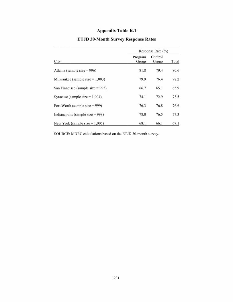
231
Appendix Table K.1
ETJD 30-Month Survey Response Rates
Response Rate (%)
Program Control City Group Group Total
Atlanta (sample size = 996) 81.8 79.4 80.6
Milwaukee (sample size = 1,003) 79.9 76.4 78.2
San Francisco (sample size = 995) 66.7 65.1 65.9
Syracuse (sample size = 1,004) 74.1 72.9 73.5
Fort Worth (sample size = 999) 76.3 76.8 76.6
Indianapolis (sample size = 998) 78.0 76.5 77.3
New York (sample size = 1,005) 68.1 66.1 67.1
SOURCE: MDRC calculations based on the ETJD 30-month survey.
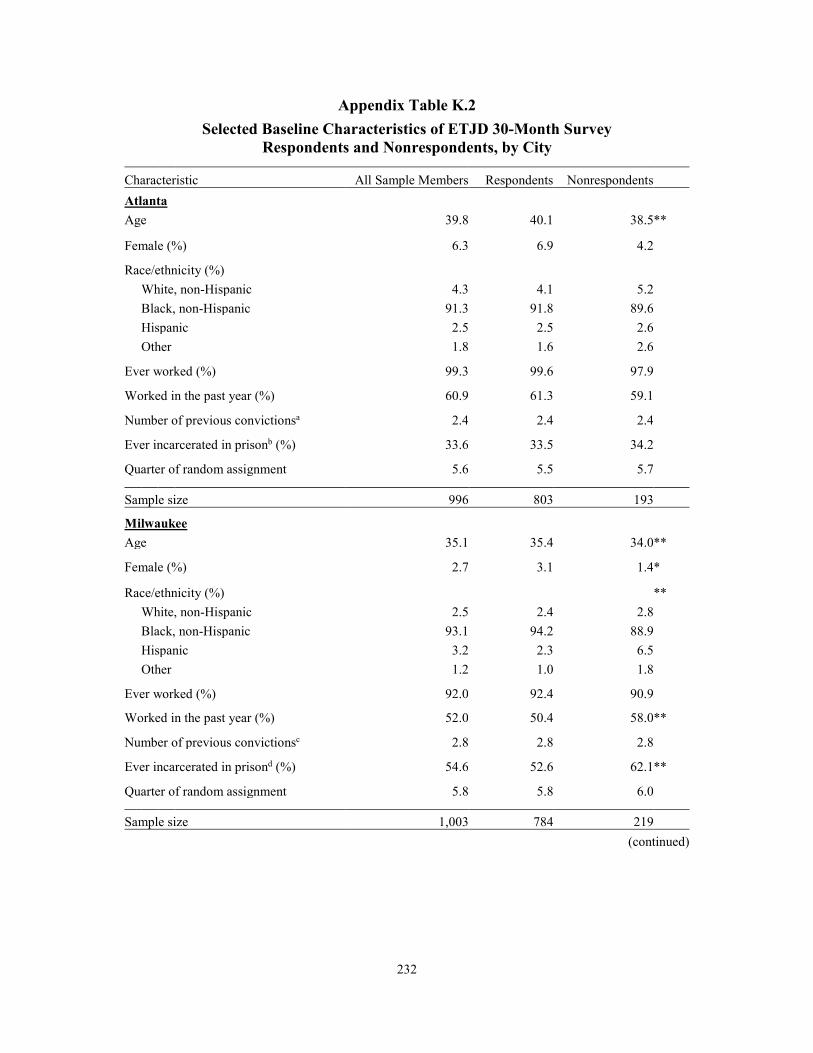
232
Appendix Table K.2
a
b
(continued)
Selected Baseline Characteristics of ETJD 30-Month Survey Respondents and Nonrespondents, by City
Characteristic All Sample Members Respondents Nonrespondents Atlanta Age 39.8 40.1 38.5 **
Female (%) 6.3 6.9 4.2 Race/ethnicity (%)
White, non-Hispanic 4.3 4.1 5.2 Black, non-Hispanic 91.3 91.8 89.6 Hispanic 2.5 2.5 2.6 Other 1.8 1.6 2.6
Ever worked (%) 99.3 99.6 97.9 Worked in the past year (%) 60.9 61.3 59.1 Number of previous convictions 2.4 2.4 2.4 Ever incarcerated in prison (%) 33.6 33.5 34.2 Quarter of random assignment 5.6 5.5 5.7
Sample size 996 803 193
Milwaukee Age 35.1 35.4 34.0 **
Female (%) 2.7 3.1 1.4 *
Race/ethnicity (%) ** White, non-Hispanic 2.5 2.4 2.8 Black, non-Hispanic 93.1 94.2 88.9 Hispanic 3.2 2.3 6.5 Other 1.2 1.0 1.8
Ever worked (%) 92.0 92.4 90.9 Worked in the past year (%) 52.0 50.4 58.0 **
Number of previous convictionsc 2.8 2.8 2.8 Ever incarcerated in prisond (%) 54.6 52.6 62.1 **
Quarter of random assignment 5.8 5.8 6.0
Sample size 1,003 784 219
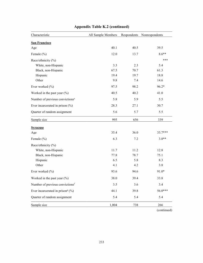
233
Appendix Table K.2 (continued)
Characteristic All Sample Members Respondents Nonrespondents
e
(continued)
San Francisco Age 40.1 40.5 39.5
Female (%) 12.0 13.7 8.6 **
Race/ethnicity (%) *** White, non-Hispanic 3.3 2.3 5.4 Black, non-Hispanic 67.5 70.7 61.3 Hispanic 19.4 19.7 18.8 Other 9.8 7.4 14.6
Ever worked (%) 97.5 98.2 96.2 * Worked in the past year (%) 40.5 40.2 41.0
Number of previous convictions 5.8 5.9 5.5
Ever incarcerated in prison (%) 28.3 27.1 30.7
Quarter of random assignment 5.6 5.7 5.5
Sample size 995 656 339
Syracuse Age 35.4 36.0 33.7 ***
Female (%) 6.3 7.2 3.8 **
Race/ethnicity (%) White, non-Hispanic 11.7 11.2 12.8 Black, non-Hispanic 77.8 78.7 75.1 Hispanic 6.5 5.8 8.3 Other 4.1 4.2 3.8
Ever worked (%) 93.6 94.6 91.0 *
Worked in the past year (%) 38.0 39.4 33.8
Number of previous convictionsf 3.5 3.6 3.4
Ever incarcerated in prisong (%) 44.1 39.8 56.0 *** Quarter of random assignment 5.4 5.4 5.4
Sample size 1,004 738 266
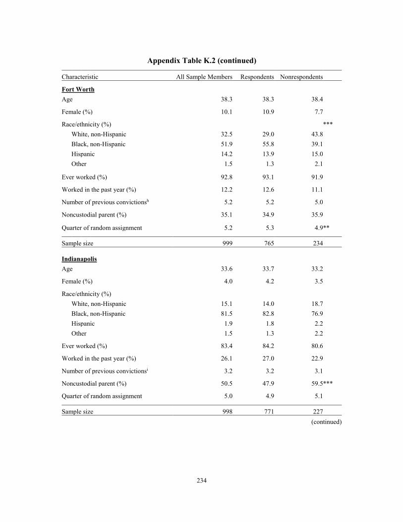
234
Appendix Table K.2 (continued)
(continued)
Characteristic All Sample Members Respondents Nonrespondents
Fort Worth Age 38.3 38.3 38.4
Female (%) 10.1 10.9 7.7
Race/ethnicity (%) *** White, non-Hispanic 32.5 29.0 43.8 Black, non-Hispanic 51.9 55.8 39.1 Hispanic 14.2 13.9 15.0 Other 1.5 1.3 2.1
Ever worked (%) 92.8 93.1 91.9
Worked in the past year (%) 12.2 12.6 11.1
Number of previous convictionsh 5.2 5.2 5.0
Noncustodial parent (%) 35.1 34.9 35.9
Quarter of random assignment 5.2 5.3 4.9 **
Sample size 999 765 234
Indianapolis Age 33.6 33.7 33.2
Female (%) 4.0 4.2 3.5
Race/ethnicity (%) White, non-Hispanic 15.1 14.0 18.7 Black, non-Hispanic 81.5 82.8 76.9 Hispanic 1.9 1.8 2.2 Other 1.5 1.3 2.2
Ever worked (%) 83.4 84.2 80.6
Worked in the past year (%) 26.1 27.0 22.9
Number of previous convictionsi 3.2 3.2 3.1
Noncustodial parent (%) 50.5 47.9 59.5 ***
Quarter of random assignment 5.0 4.9 5.1
Sample size 998 771 227
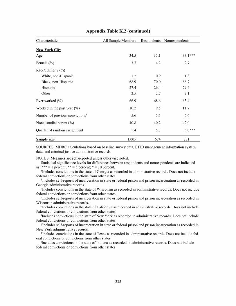
235
Appendix Table K.2 (continued)
Characteristic All Sample Members Respondents Nonrespondents
f
New York City Age 34.5 35.1 33.1 ***
Female (%) 3.7 4.2 2.7
Race/ethnicity (%) White, non-Hispanic 1.2 0.9 1.8 Black, non-Hispanic 68.9 70.0 66.7 Hispanic 27.4 26.4 29.4 Other 2.5 2.7 2.1
Ever worked (%) 66.9 68.6 63.4
Worked in the past year (%) 10.2 9.5 11.7
Number of previous convictions 5.6 5.5 5.6
Noncustodial parent (%) 40.8 40.2 42.0
Quarter of random assignment 5.4 5.7 5.0 ***
Sample size 1,005 674 331
SOURCES: MDRC calculations based on baseline survey data, ETJD management information system data, and criminal justice administrative records.
NOTES: Measures are self-reported unless otherwise noted. Statistical significance levels for differences between respondents and nonrespondents are indicated as: *** = 1 percent; ** = 5 percent; * = 10 percent. aIncludes convictions in the state of Georgia as recorded in administrative records. Does not include federal convictions or convictions from other states. bIncludes self-reports of incarceration in state or federal prison and prison incarceration as recorded in Georgia administrative records. cIncludes convictions in the state of Wisconsin as recorded in administrative records. Does not include federal convictions or convictions from other states. dIncludes self-reports of incarceration in state or federal prison and prison incarceration as recorded in Wisconsin administrative records. eIncludes convictions in the state of California as recorded in administrative records. Does not include federal convictions or convictions from other states. fIncludes convictions in the state of New York as recorded in administrative records. Does not include federal convictions or convictions from other states. gIncludes self-reports of incarceration in state or federal prison and prison incarceration as recorded in New York administrative records. hIncludes convictions in the state of Texas as recorded in administrative records. Does not include fed-eral convictions or convictions from other states. iIncludes convictions in the state of Indiana as recorded in administrative records. Does not include federal convictions or convictions from other states.
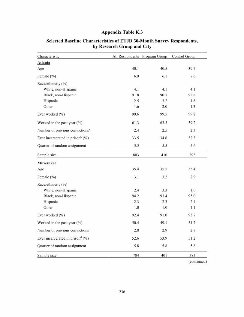
236
Appendix Table K.3
d
(continued)
Selected Baseline Characteristics of ETJD 30-Month Survey Respondents, by Research Group and City
Characteristic All Respondents Program Group Control Group Atlanta Age 40.1 40.5 39.7
Female (%) 6.9 6.1 7.6 Race/ethnicity (%)
White, non-Hispanic 4.1 4.1 4.1 Black, non-Hispanic 91.8 90.7 92.8 Hispanic 2.5 3.2 1.8 Other 1.6 2.0 1.3
Ever worked (%) 99.6 99.5 99.8
Worked in the past year (%) 61.3 63.3 59.2
Number of previous convictionsa 2.4 2.5 2.3
Ever incarcerated in prisonb (%) 33.5 34.6 32.3
Quarter of random assignment 5.5 5.5 5.6
Sample size 803 410 393
Milwaukee Age 35.4 35.5 35.4
Female (%) 3.1 3.2 2.9 Race/ethnicity (%)
White, non-Hispanic 2.4 3.3 1.6 Black, non-Hispanic 94.2 93.4 95.0 Hispanic 2.3 2.3 2.4 Other 1.0 1.0 1.1
Ever worked (%) 92.4 91.0 93.7
Worked in the past year (%) 50.4 49.1 51.7
Number of previous convictionsc 2.8 2.9 2.7
Ever incarcerated in prison (%) 52.6 53.9 51.2
Quarter of random assignment 5.8 5.8 5.8
Sample size 784 401 383
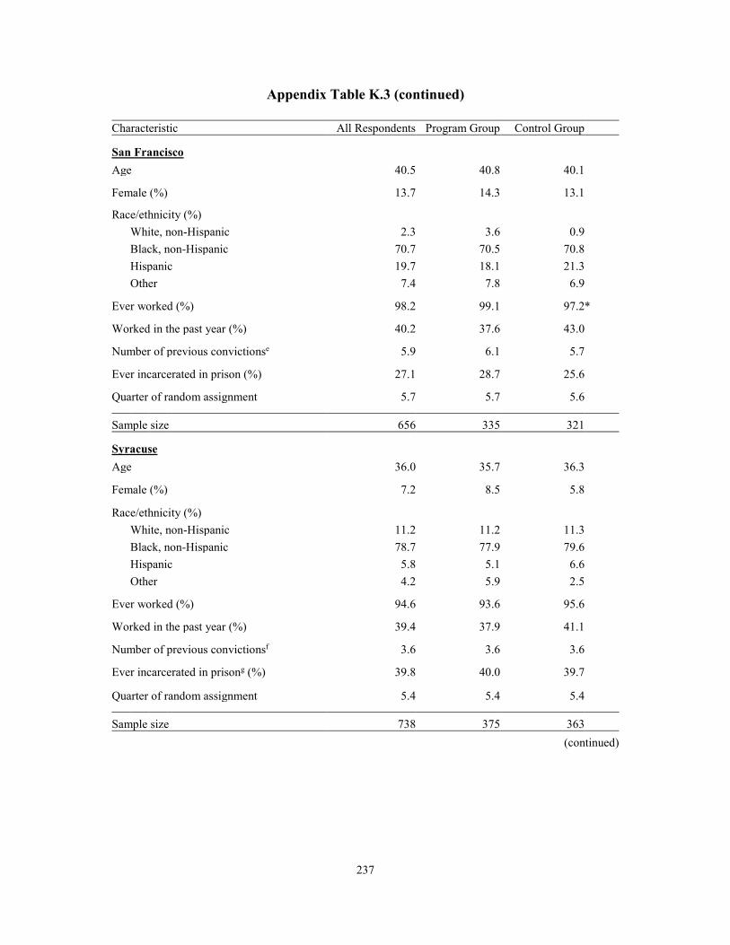
237
Appendix Table K.3 (continued)
Characteristic All Respondents Program Group Control Group
(continued)
San Francisco Age 40.5 40.8 40.1
Female (%) 13.7 14.3 13.1 Race/ethnicity (%)
White, non-Hispanic 2.3 3.6 0.9 Black, non-Hispanic 70.7 70.5 70.8 Hispanic 19.7 18.1 21.3 Other 7.4 7.8 6.9
Ever worked (%) 98.2 99.1 97.2 *
Worked in the past year (%) 40.2 37.6 43.0
Number of previous convictionse 5.9 6.1 5.7
Ever incarcerated in prison (%) 27.1 28.7 25.6
Quarter of random assignment 5.7 5.7 5.6
Sample size 656 335 321
Syracuse Age 36.0 35.7 36.3
Female (%) 7.2 8.5 5.8
Race/ethnicity (%) White, non-Hispanic 11.2 11.2 11.3 Black, non-Hispanic 78.7 77.9 79.6 Hispanic 5.8 5.1 6.6 Other 4.2 5.9 2.5
Ever worked (%) 94.6 93.6 95.6
Worked in the past year (%) 39.4 37.9 41.1
Number of previous convictionsf 3.6 3.6 3.6
Ever incarcerated in prisong (%) 39.8 40.0 39.7
Quarter of random assignment 5.4 5.4 5.4
Sample size 738 375 363
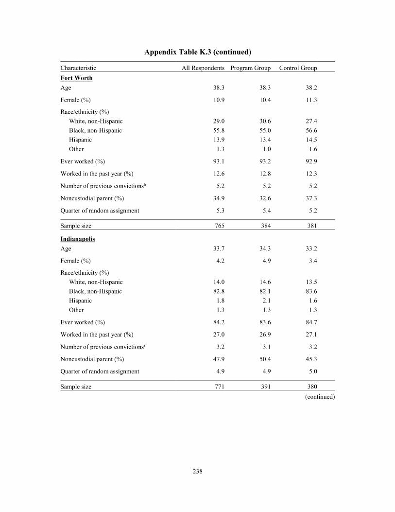
238
Appendix Table K.3 (continued)
Characteristic All Respondents Program Group Control Group
(continued)
Fort Worth Age 38.3 38.3 38.2
Female (%) 10.9 10.4 11.3 Race/ethnicity (%)
White, non-Hispanic 29.0 30.6 27.4 Black, non-Hispanic 55.8 55.0 56.6 Hispanic 13.9 13.4 14.5 Other 1.3 1.0 1.6
Ever worked (%) 93.1 93.2 92.9
Worked in the past year (%) 12.6 12.8 12.3
Number of previous convictionsh 5.2 5.2 5.2
Noncustodial parent (%) 34.9 32.6 37.3
Quarter of random assignment 5.3 5.4 5.2
Sample size 765 384 381
Indianapolis Age 33.7 34.3 33.2
Female (%) 4.2 4.9 3.4 Race/ethnicity (%)
White, non-Hispanic 14.0 14.6 13.5 Black, non-Hispanic 82.8 82.1 83.6 Hispanic 1.8 2.1 1.6 Other 1.3 1.3 1.3
Ever worked (%) 84.2 83.6 84.7
Worked in the past year (%) 27.0 26.9 27.1
Number of previous convictionsi 3.2 3.1 3.2
Noncustodial parent (%) 47.9 50.4 45.3
Quarter of random assignment 4.9 4.9 5.0
Sample size 771 391 380
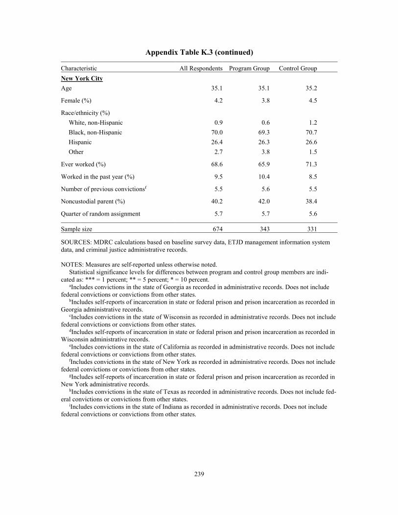
239
Appendix Table K.3 (continued)
Characteristic All Respondents Program Group Control Group
New York City Age 35.1 35.1 35.2
Female (%) 4.2 3.8 4.5
Race/ethnicity (%) White, non-Hispanic 0.9 0.6 1.2 Black, non-Hispanic 70.0 69.3 70.7 Hispanic 26.4 26.3 26.6 Other 2.7 3.8 1.5
Ever worked (%) 68.6 65.9 71.3
Worked in the past year (%) 9.5 10.4 8.5
Number of previous convictionsf 5.5 5.6 5.5
Noncustodial parent (%) 40.2 42.0 38.4
Quarter of random assignment 5.7 5.7 5.6
Sample size 674 343 331
SOURCES: MDRC calculations based on baseline survey data, ETJD management information system data, and criminal justice administrative records.
NOTES: Measures are self-reported unless otherwise noted. Statistical significance levels for differences between program and control group members are indi-cated as: *** = 1 percent; ** = 5 percent; * = 10 percent. aIncludes convictions in the state of Georgia as recorded in administrative records. Does not include federal convictions or convictions from other states. bIncludes self-reports of incarceration in state or federal prison and prison incarceration as recorded in Georgia administrative records. cIncludes convictions in the state of Wisconsin as recorded in administrative records. Does not include federal convictions or convictions from other states. dIncludes self-reports of incarceration in state or federal prison and prison incarceration as recorded in Wisconsin administrative records. eIncludes convictions in the state of California as recorded in administrative records. Does not include federal convictions or convictions from other states. fIncludes convictions in the state of New York as recorded in administrative records. Does not include federal convictions or convictions from other states. gIncludes self-reports of incarceration in state or federal prison and prison incarceration as recorded in New York administrative records. hIncludes convictions in the state of Texas as recorded in administrative records. Does not include fed-eral convictions or convictions from other states. iIncludes convictions in the state of Indiana as recorded in administrative records. Does not include federal convictions or convictions from other states.
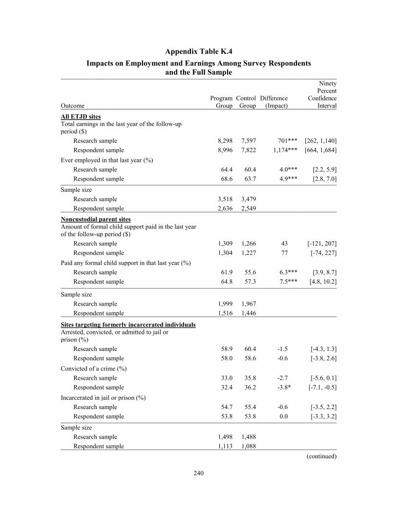
240
(continued)
Appendix Table K.4
Impacts on Employment and Earnings Among Survey Respondents and the Full Sample
Outcome
Program Group
Control Group
Difference (Impact)
Ninety Percent
Confidence Interval
All ETJD sites Total earnings in the last year of the follow-up period ($)
Research sample 8,298 7,597 701 *** [262, 1,140] Respondent sample 8,996 7,822 1,174 *** [664, 1,684]
Ever employed in that last year (%) Research sample 64.4 60.4 4.0 *** [2.2, 5.9] Respondent sample 68.6 63.7 4.9 *** [2.8, 7.0]
Sample size Research sample 3,518 3,479 Respondent sample 2,636 2,549
Noncustodial parent sites Amount of formal child support paid in the last year of the follow-up period ($)
Research sample 1,309 1,266 43 [-121, 207] Respondent sample 1,304 1,227 77 [-74, 227]
Paid any formal child support in that last year (%) Research sample 61.9 55.6 6.3 *** [3.9, 8.7] Respondent sample 64.8 57.3 7.5 *** [4.8, 10.2]
Sample size Research sample 1,999 1,967 Respondent sample 1,516 1,446
Sites targeting formerly incarcerated individuals Arrested, convicted, or admitted to jail or prison (%)
Research sample 58.9 60.4 -1.5 [-4.3, 1.3] Respondent sample 58.0 58.6 -0.6 [-3.8, 2.6]
Convicted of a crime (%) Research sample 33.0 35.8 -2.7 [-5.6, 0.1] Respondent sample 32.4 36.2 -3.8 * [-7.1, -0.5]
Incarcerated in jail or prison (%) Research sample 54.7 55.4 -0.6 [-3.5, 2.2] Respondent sample 53.8 53.8 0.0 [-3.3, 3.2]
Sample size Research sample 1,498 1,488 Respondent sample 1,113 1,088
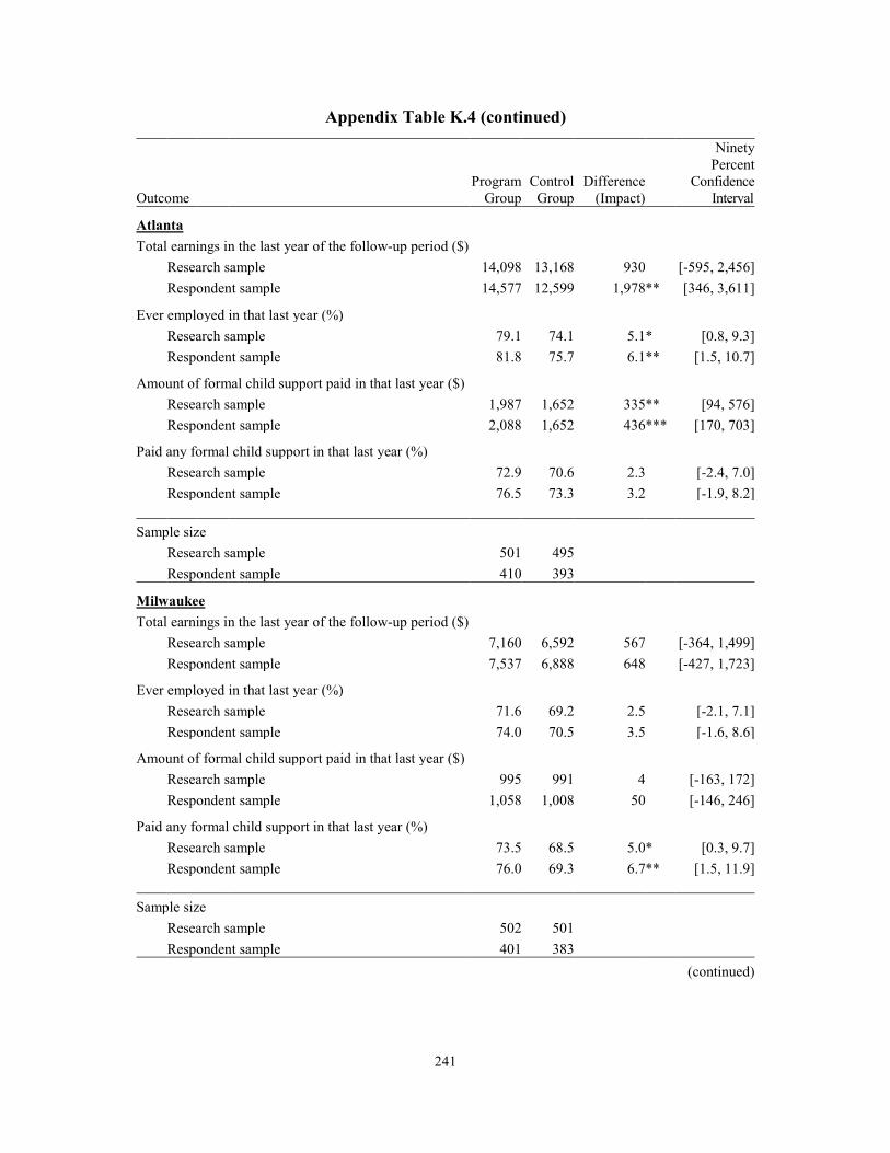
241
Appendix Table K.4 (continued)
Outcome Program
Group Control
Group Difference
(Impact)
NinetyPercent
ConfidenceInterval
Atlanta Total earnings in the last year of the follow-up period ($)
(continued)
Research sample 14,098 13,168 930 [-595, 2,456] Respondent sample 14,577 12,599 1,978 ** [346, 3,611]
Ever employed in that last year (%) Research sample 79.1 74.1 5.1 * [0.8, 9.3] Respondent sample 81.8 75.7 6.1 ** [1.5, 10.7]
Amount of formal child support paid in that last year ($) Research sample 1,987 1,652 335 ** [94, 576] Respondent sample 2,088 1,652 436 *** [170, 703]
Paid any formal child support in that last year (%) Research sample 72.9 70.6 2.3 [-2.4, 7.0] Respondent sample 76.5 73.3 3.2 [-1.9, 8.2]
Sample size Research sample 501 495 Respondent sample 410 393
Milwaukee Total earnings in the last year of the follow-up period ($)
Research sample 7,160 6,592 567 [-364, 1,499] Respondent sample 7,537 6,888 648 [-427, 1,723]
Ever employed in that last year (%) Research sample 71.6 69.2 2.5 [-2.1, 7.1] Respondent sample 74.0 70.5 3.5 [-1.6, 8.6]
Amount of formal child support paid in that last year ($) Research sample 995 991 4 [-163, 172] Respondent sample 1,058 1,008 50 [-146, 246]
Paid any formal child support in that last year (%) Research sample 73.5 68.5 5.0 * [0.3, 9.7] Respondent sample 76.0 69.3 6.7 ** [1.5, 11.9]
Sample size Research sample 502 501 Respondent sample 401 383
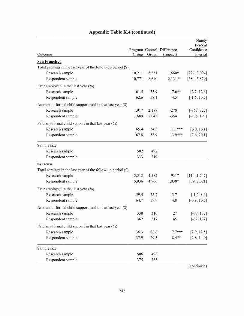
242
Appendix Table K.4 (continued)
Outcome Program
Group Control
Group Difference
(Impact)
Ninety Percent
Confidence Interval
San Francisco Total earnings in the last year of the follow-up period ($)
(continued)
Research sample 10,211 8,551 1,660 * [227, 3,094] Respondent sample 10,771 8,640 2,131 ** [384, 3,879]
Ever employed in that last year (%) Research sample 61.5 53.9 7.6 ** [2.7, 12.6] Respondent sample 62.6 58.1 4.5 [-1.6, 10.7]
Amount of formal child support paid in that last year ($) Research sample 1,917 2,187 -270 [-867, 327] Respondent sample 1,689 2,043 -354 [-905, 197]
Paid any formal child support in that last year (%) Research sample 65.4 54.3 11.1 *** [6.0, 16.1] Respondent sample 67.8 53.9 13.9 *** [7.6, 20.1]
Sample size Research sample 502 492 Respondent sample 333 319
Syracuse Total earnings in the last year of the follow-up period ($)
Research sample 5,513 4,582 931 * [114, 1,747] Respondent sample 5,936 4,906 1,030 * [39, 2,021]
Ever employed in that last year (%) Research sample 59.4 55.7 3.7 [-1.2, 8.6] Respondent sample 64.7 59.9 4.8 [-0.9, 10.5]
Amount of formal child support paid in that last year ($) Research sample 338 310 27 [-78, 132] Respondent sample 362 317 45 [-82, 172]
Paid any formal child support in that last year (%) Research sample 36.3 28.6 7.7 *** [2.9, 12.5] Respondent sample 37.9 29.5 8.4 ** [2.8, 14.0]
Sample size Research sample 506 498 Respondent sample 375 363
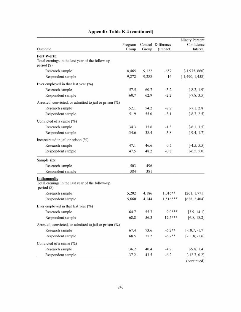
243
(continued)
Appendix Table K.4 (continued)
Outcome Program
Group Control
Group Difference
(Impact)
Ninety Percent Confidence
Interval
Fort Worth Total earnings in the last year of the follow-up period ($)
Research sample 8,465 9,122 -657 [-1,975, 660] Respondent sample 9,272 9,288 -16 [-1,490, 1,458]
Ever employed in that last year (%) Research sample 57.5 60.7 -3.2 [-8.2, 1.9] Respondent sample 60.7 62.9 -2.2 [-7.8, 3.5]
Arrested, convicted, or admitted to jail or prison (%) Research sample 52.1 54.2 -2.2 [-7.1, 2.8] Respondent sample 51.9 55.0 -3.1 [-8.7, 2.5]
Convicted of a crime (%) Research sample 34.3 35.6 -1.3 [-6.1, 3.5] Respondent sample 34.6 38.4 -3.8 [-9.4, 1.7]
Incarcerated in jail or prison (%) Research sample 47.1 46.6 0.5 [-4.5, 5.5] Respondent sample 47.5 48.2 -0.8 [-6.5, 5.0]
Sample size Research sample 503 496 Respondent sample 384 381
Indianapolis Total earnings in the last year of the follow-up period ($)
Research sample 5,202 4,186 1,016 ** [261, 1,771] Respondent sample 5,660 4,144 1,516 *** [628, 2,404]
Ever employed in that last year (%) Research sample 64.7 55.7 9.0 *** [3.9, 14.1] Respondent sample 68.8 56.3 12.5 *** [6.8, 18.2]
Arrested, convicted, or admitted to jail or prison (%) Research sample 67.4 73.6 -6.2 ** [-10.7, -1.7] Respondent sample 68.5 75.2 -6.7 ** [-11.8, -1.6]
Convicted of a crime (%) Research sample 36.2 40.4 -4.2 [-9.8, 1.4] Respondent sample 37.2 43.5 -6.2 [-12.7, 0.2]
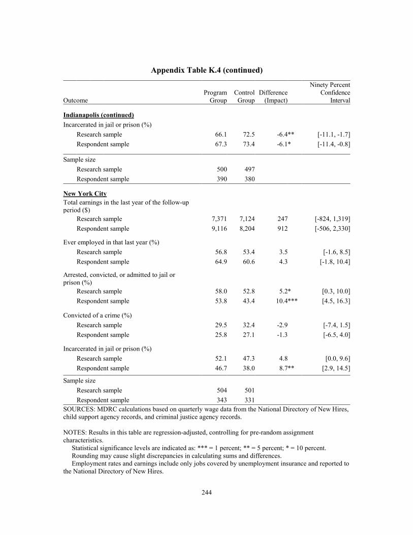
244
Appendix Table K.4 (continued)
Outcome Program
Group Control
Group Difference
(Impact)
Ninety Percent Confidence
Interval
Indianapolis (continued) Incarcerated in jail or prison (%)
Research sample Respondent sample
66.1 67.3
72.5 73.4
-6.4 ** -6.1 *
[-11.1, [-11.4,
-1.7] -0.8]
Sample size Research sample Respondent sample
500 390
497 380
New York City Total earnings in the last year of the follow-up period ($)
Research sample Respondent sample
Ever employed in that last year (%) Research sample Respondent sample
Arrested, convicted, or admitted to jail or prison (%)
Research sample Respondent sample
Convicted of a crime (%) Research sample Respondent sample
Incarcerated in jail or prison (%) Research sample Respondent sample
7,371 9,116
56.8 64.9
58.0 53.8
29.5 25.8
52.1 46.7
7,124 8,204
53.4 60.6
52.8 43.4
32.4 27.1
47.3 38.0
247 912
3.5 4.3
5.2 * 10.4 ***
-2.9 -1.3
4.8 8.7 **
[-824, 1,319] [-506, 2,330]
[-1.6, 8.5] [-1.8, 10.4]
[0.3, 10.0] [4.5, 16.3]
[-7.4, 1.5] [-6.5, 4.0]
[0.0, 9.6] [2.9, 14.5]
Sample size Research sample Respondent sample
504 343
501 331
SOURCES: MDRC calculations based on quarterly wage data from the National Directory of New Hires, child support agency records, and criminal justice agency records.
NOTES: Results in this table are regression-adjusted, controlling for pre-random assignment characteristics. Statistical significance levels are indicated as: *** = 1 percent; ** = 5 percent; * = 10 percent. Rounding may cause slight discrepancies in calculating sums and differences. Employment rates and earnings include only jobs covered by unemployment insurance and reported to the National Directory of New Hires.

Appendix L
The Analytic Approach to Determining Impacts Among Recidivism-Risk Subgroups

THIS PAGE INTENTIONALLY LEFT BLANK
247
The methodological approach used for determining whether impacts vary with study participants’ risk of recidivism draws on the approach described in Zweig, Yahner, and Redcross (2010).1 It focuses on formerly incarcerated individuals’ probability of rearrest, reconviction, and reincar-ceration in the 30 months following random assignment.2 The research goal is to differentiate formerly incarcerated individuals into lower-to-moderate-risk and higher-risk subgroups, depend-ing on their risk of recidivism as predicted before study participation, and then to examine the impact each Enhanced Transitional Jobs Demonstration (ETJD) program targeting formerly in-carcerated individuals had on each subgroup’s recidivism.
Given the random assignment research design of the evaluation, the observed and un-observed baseline characteristics of study sample members assigned to the control group should reflect, on average, those of sample members assigned to the program group. The evaluation cap-italizes on the opportunity presented by experimental data to estimate the risk of recidivism among formerly incarcerated individuals in the program group, using characteristics measured before program participation, based on observations of such risk in the control group. It then classifies participants into lower-to-moderate-risk and higher-risk subgroups based on these risk scores and evaluates the impact of the Fort Worth, Indianapolis, and New York City ETJD pro-grams on recidivism within each subgroup.
Toward this end, the analytic strategy is threefold. The first step is to examine the predic-tive associations between all baseline characteristics and recidivism in the year after random as-signment for each site. The candidate covariates (predictors) were the covariates used for the full sample impact models presented through this report.3 For this analysis, a bootstrap validation procedure was employed to derive the best-fitting, most parsimonious model to predict recidivism risk (1) among the pooled sample from the three sites targeting formerly incarcerated individuals (Fort Worth, Indianapolis, and New York City) and (2) at each of the these three sites. The boot-strap procedure was implemented as follows:
1. Generate 100 bootstrap samples (sample with replacement) from the control group data.
1The Zweig, Yahner, and Redcross approach is a modified version of the procedure described in Kemple
and Snipes (2001). 2Recidivism in this analysis is defined as having any criminal justice event in the 30 months following
random assignment. This measure of “any criminal justice event,” featured elsewhere in this report, is derived from state and local criminal justice records covering arrests, convictions, jail admissions, and prison admissions.
3The two work-experience covariates — (1) having ever worked and (2) having worked in the year before random assignment — were combined into a single work-experience variable with three categories: (1) never worked, (2) worked earlier than the year before random assignment but not during the year before random as-signment, and (3) worked during the year before random assignment. These changes were made to simplify model estimation.
248
2. Estimate the model from each bootstrap sample using stepwise selection.
3. Estimate model optimism by comparing model performance with the boot- strap sample and the original sample.4
The final model covariates are determined by examining the covariates selected in each of the bootstrap models. If a variable is “truly” representative of the model it will occur in the majority of the bootstrap models (in at least 50 of the 100 models). Overall accuracy is indicated by a summary of the bootstrap model optimism estimates. Model performance is assessed using the “c” statistic (the area under the receiver operating characteristic curve, or “AUC”), which provides an overall measure of how well the model correctly classifies the outcome.5
The results showed that the models were able to accurately predict recidivism about 72 percent of the time in the pooled sample, about 70 percent of the time in Fort Worth, 68 percent of the time in Indianapolis, and 72 percent of the time in New York City, and that the potential bias due to overfitting in each case was small.6
The analysis culminated by identifying participants’ ages and numbers of previous con-victions as important predictors of recidivism in the pooled sample’s model and in all three sites’ models; months incarcerated before a person entered the study as important predictors of recidi-vism in the pooled-sample, Fort Worth, and New York City models; quarter of random assign-ment as an important predictor of recidivism in the Fort Worth model; and gender and site as important predictors of recidivism in the pooled sample’s model.7 At each of the three sites and
4An important threat to the validity of the predictions for new subjects is overfitting: the possibility that a
given model is not generalizable due to specifics and idiosyncrasies in the sample. Overfitting leads to an optimistic impression of model performance for the purposes of generating predictions in new subjects.
5AUC is problematic when comparing competing model specifications (Hand, 2009; Hand and Anagnos-topoulos, 2013), but it is used here to compare one model across data sets (bootstrap sample versus original sample).
6In the pooled sample from the three sites targeting formerly incarcerated individuals, on average, the AUC for the bootstrap samples (corrected for optimism) was 0.72, ranging from 0.69 to 0.76 with a mean optimism correction of 0.04. In Fort Worth, on average, the AUC for the bootstrap samples (corrected for optimism) was 0.70, ranging from 0.65 to 0.76 with a mean optimism correction of 0.02. In Indianapolis, on average, the AUC for the bootstrap samples (corrected for optimism) was 0.68, ranging from 0.59 to 0.75 with a mean optimism correction of 0.02. In New York City, on average, the AUC for the bootstrap samples (corrected for optimism) was 0.72, ranging from 0.66 to 0.78 with a mean optimism correction of 0.02.
7Age appeared in all 100 bootstrap models for the pooled sample, Fort Worth, and New York, and in 99 of the 100 bootstrap models for Indianapolis. Number of previous convictions appeared in all 100 of the bootstrap models for the pooled sample, Fort Worth, and New York, and in 94 of the 100 bootstrap models for Indianapolis. Months incarcerated (including months in both prison and jail) appeared in all 100 of the bootstrap models for Fort Worth, 97 of the 100 bootstrap models for New York, and 87 of the 100 bootstrap models for the pooled sample. Quarter of random assignment appeared in 70 of the 100 bootstrap models for Fort Worth. Gender

249
within the pooled sample, older sample members were less likely to reoffend than younger sample members, all else being equal. Also, sample members with more previous convictions were more likely to reoffend than those with fewer previous convictions. In Fort Worth, New York City, and the pooled sample, sample members who had spent more months incarcerated were more likely to reoffend that those who had spent fewer months incarcerated. In Fort Worth, sample members who entered the study later were more likely to reoffend than those who entered earlier. In the pooled sample, women were less likely to reoffend than men, and individuals in Indianapolis were more likely to reoffend than individuals in Fort Worth and New York City.8
The second step is to estimate the probability (risk) of recidivism for the full sample, by applying the estimated regression coefficients from the bootstrapping model parameters to both the program group and the control group at each site and within the pooled sample. For each study participant at a site and within the pooled sample, a risk-of-recidivism score is generated and used to create subgroups of lower-to-moderate-risk and higher-risk offenders.9 The distribution of risk scores for the control group was examined to identify the seventy-fifth-percentile scores at each site and within the pooled sample. Participants with risk scores lower than the seventy-fifth per-centile at their site are said to be at lower to moderate risk of reoffending within that site, while those with risk scores above the seventy-fifth percentile at their site are said to be at higher risk. Similarly, participants with risk scores lower than the seventy-fifth percentile in the pooled sam-ple (the combined sample from all three sites targeting formerly incarcerated individuals) are said to be at lower to moderate risk of reoffending within the pooled sample, while those with risk scores above the seventy-fifth percentile in the pooled sample are said to be at higher risk.
The third and final step is to analyze the impact of each ETJD program targeting formerly incarcerated people within each subgroup by estimating a series of regression models. Each out-come model uses the same predictors as those in the model estimating risk scores but includes an additional variable measuring ETJD program group status. From each model’s output, adjusted outcomes are generated for the program and control participants to show the size of the ETJD program’s impact, while determining the significance of the impact by the p-value associated with the program variable’s coefficient in each outcome model. This analysis is performed for each of the three individual sites and for the pooled sample.
appeared in 81 of the 100 bootstrap models for the pooled sample. Site (an indicator for ETJD program site) appeared in all 100 bootstrap models for the pooled sample.
8As discussed in more detail in Chapter 4 of this report, this finding is consistent with the Indianapolis pro-gram serving a higher-risk population than those served by the programs in Fort Worth and New York City.
9So that results can be more easily interpreted and presented for use by practitioners, the study takes a subgroup-based approach rather than using the continuous risk-score index.

THIS PAGE INTENTIONALLY LEFT BLANK

Appendix M
Extended Follow-Up

THIS PAGE INTENTIONALLY LEFT BLANK
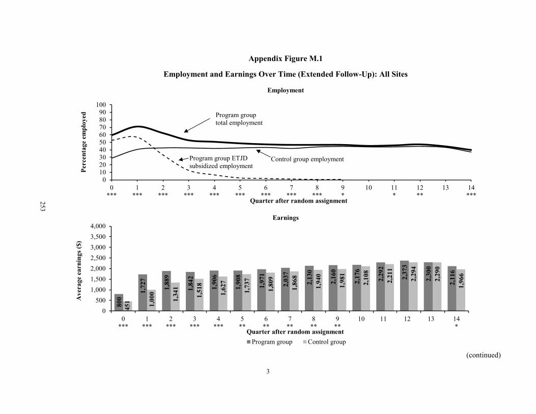
3
(continued)
Appendix Figure M.1
Employment and Earnings Over Time (Extended Follow-Up): All Sites
Employment
Earnings
0102030405060708090
100
0***
1***
2***
3***
4***
5***
6***
7***
8***
9*
10 11*
12**
13 14***
Perc
enta
ge e
mpl
oyed
Quarter after random assignment
Program group total employment
Control group employment
800
1,72
7
1,88
9
1,84
2
1,90
6
1,90
8
1,97
1
2,03
7
2,13
0
2,16
0
2,17
6
2,29
2
2,37
3
2,30
0
2,11
6
451 1,00
0
1,34
1
1,51
8
1,62
7
1,73
7
1,80
9
1,86
8
1,94
0
1,98
1
2,10
8
2,21
1
2,29
4
2,29
0
1,96
6
0500
1,0001,5002,0002,5003,0003,5004,000
0***
1***
2***
3***
4***
5**
6**
7**
8**
9**
10 11 12 13 14*
Ave
rage
ear
ning
s ($)
Quarter after random assignmentProgram group Control group
Program group ETJDsubsidized employment
253

254
SOURCES: MDRC calculations based on quarterly wage data from the National Directory of New Hires and program payroll records.
NOTES: Results in this figure are regression-adjusted, controlling for pre-random assignment characteristics. Statistical significance levels are indicated as: *** = 1 percent; ** = 5 percent; * = 10 percent. Employment rates and earnings in the quarter of random assignment through Quarter 5 after random assignment include both ETJD subsidized jobs and jobs covered by unemployment insurance and re-ported to the National Directory of New Hires. Employment rates and earnings in Quarters 6 through 14 after random assignment include only jobs covered by unemployment insurance and reported to the Na-tional Directory of New Hires.
Appendix Figure M.1 (continued)
255
References
Amato, Paul, and Joan Gilbreth. 1999. “Nonresident Fathers and Children’s Well-Being: A Meta-Analysis.” Journal of Marriage and the Family 61, 3: 557-573.
Butler, David, Julianna Alson, Dan Bloom, Victoria Deitch, Aaron Hill, JoAnn Hsueh, Erin Jacobs Valentine, Sue Kim, Reanin McRoberts, and Cindy Redcross. 2012. What Strategies Work for the Hard-to-Employ? Final Results of the Hard-to-Employ Demonstration and Evaluation Project and Selected Sites from the Employment Retention and Advancement Project. New York: MDRC.
Cancian, Maria, Carolyn J. Heinrich, and Yiyoon Chung. 2013. “Discouraging Disadvantaged Fathers’ Employment: An Unintended Consequence of Policies Designed to Support Families.” Journal of Policy Analysis and Management 32, 4: 758-784.
Caron, E. Ann, and William J. Sabol. 2012. Prisoners in 2011. Washington, DC: U.S. Department of Justice, Bureau of Justice Statistics.
Duran, Le’Ann, Martha Plotkin, Phoebe Potter, and Henry Rosen. 2013. Integrated Reentry and Employment Strategies: Reducing Recidivism and Promoting Job Readiness. New York: Council of State Governments Justice Center.
Durose, Matthew, Alexia D. Cooper, and Howard N. Snyder. 2014. “Recidivism of Prisoners Released in 30 States in 2005: Patterns from 2005 to 2010.” Washington, DC: U.S. Department of Justice, Bureau of Justice Statistics.
Dutta-Gupta, Indivar, Kali Grant, Matthew Eckel, and Peder Edelman. 2016. Lessons Learned from 40 Years of Subsidized Employment Programs: A Framework, Review of Models, and Recommendations for Helping Disadvantaged Workers. Washington, DC: Georgetown Center on Poverty and Inequality.
Foley, Kimberly, Mary Farrell, Riley Webster, and Johanna Walter. Forthcoming. Reducing Recidivism and Increasing Opportunity: Benefits and Costs of the RecycleForce Enhanced Transitional Jobs Program. New York: MDRC.
Glosser, Asaph, Bret Barden, and Sonya Williams, with Chloe Anderson. 2016. Testing Two Subsidized Employment Approaches for Recipients of Temporary Assistance for Needy Families: Implementation and Early Impacts of the Los Angeles County Transitional Subsidized Employment Program. OPRE Report 2016-77. Washington, DC: Office of Planning, Research, and Evaluation, Administration for Children and Families, U.S. Department of Health and Human Services.
Greenberg, David, Robert H. Meyer, and Michael Wiseman. 1994. “Multisite Employment and Training Program Evaluations: A Tale of Three Studies.” ILR Review 47, 4: 679-691.
Hand, David J. 2009. “Measuring Classifier Performance: A Coherent Alternative to the Area Under the ROC Curve.” Machine Learning 77, 1: 103-123.
256
Hand, David J., and Christoforos Anagnostopoulos. 2013 “When Is the Area Under the Receiver Operating Characteristic Curve an Appropriate Measure of Classifier Performance?” Pattern Recognition Letters 34, 5: 492-495.
Hendra, Richard, David H. Greenberg, Gayle Hamilton, Ari Oppenheim, Alexandra Pennington, Kelsey Schaberg, and Betsy L. Tessler. 2016. Encouraging Evidence on a Sector-Focused Advancement Strategy: Two-Year Impacts from the WorkAdvance Demonstration. New York: MDRC.
Holzer, Harry J., Steven Raphael, and Michael A. Stoll. 2003. “Employment Barriers Facing Ex-Offenders.” Reentry Roundtable Discussion Paper. Washington, DC: The Urban Institute.
Jacobs, Erin. 2012. Returning to Work After Prison: Final Results from the Transitional Jobs Reentry Demonstration. New York: MDRC.
Kemple, James J., and Jason C. Snipes. 2001. “A Regression-Based Strategy for Defining Subgroups in a Social Experiment.” New York: MDRC.
Krause, Eleanor, and Isabel Sawhill. 2017. What We Know and Don’t Know about Declining Labor Force Participation: A Review. Washington, DC: Center on Children and Families at Brookings, The Brookings Institution.
Latessa, Edward. 2008. “What Science Says About Designing Effective Prisoner Reentry Programs.” Website: http://wisfamilyimpact.org/wp-content/uploads/2014/10/ s_wifis26c02.pdf.
Mastri, Annalisa, and AnnaMaria McCutcheon. 2015. Costs of Services Provided by the WIA Adult and Dislocated Worker Programs. Princeton, NJ: Mathematica Policy Research.
Moser, André, Andreas E. Stuck, Rebecca A. Silliman, Patricia A. Ganz, and Kerri M. Clough-Gorr. 2012. “The Eight-Item Modified Medical Outcomes Study Social Support Survey: Psychometric Evaluation Showed Excellent Performance.” Journal of Clinical Epidemiology 65, 10: 1,107-1,116.
Nepomnyaschy, Lenna. 2007. “Child Support and Father-Child Contact: Testing Reciprocal Pathways.” Demography 44, 1: 93-112.
Pager, Devah. 2003. “The Mark of a Criminal Record.” American Journal of Sociology 108, 5: 937-975.
Petersilia, Joan. 2004. “What Works for Prisoner Reentry? Reviewing and Questioning the Evidence.” Federal Probation 68, 2: 4-8.
Redcross, Cindy, Bret Barden, Dan Bloom, Joseph Broadus, Jennifer Thompson, Sonya Williams, Sam Elkin, Randall Juras, Janae Bonsu, Ada Tso, Barbara Fink, Whitney Engstrom, Johanna Walter, Gary Reynolds, Mary Farrell, Karen Gardiner, Arielle Sherman, Melanie Skemer, Yana Kusayeva, and Sara Muller-Ravett. 2016. Implementation and Early Impacts of the Next Generation of Subsidized Employment Programs. New York: MDRC.
257
Redcross, Cindy, Dan Bloom, Gilda Azurdia, Janine Zweig, and Nancy Pindus. 2009. Transitional Jobs for Ex-Prisoners: Implementation, Two-Year Impacts, and Costs of the Center for Employment Opportunities (CEO) Prisoner Reentry Program. New York: MDRC.
Redcross, Cindy, Dan Bloom, Erin Jacobs, Michelle Manno, Sara Muller-Ravett, Kristin Seefeldt, Jennifer Yahner, Alford A. Young, Jr., and Janine Zweig. 2010. Work After Prison: One-Year Findings from the Transitional Jobs Reentry Demonstration. New York: MDRC.
Redcross, Cindy, Megan Millenky, Timothy Rudd, and Valerie Levshin. 2012. More Than a Job: Final Results of the Center for Employment Opportunities (CEO) Transitional Jobs Program. New York: MDRC.
Ross, Martha, and Natalie Holmes. 2017. Meet the Out-of-Work: Local Profiles of Jobless Adults and Strategies to Connect Them to Employment. Washington, DC: The Brookings Institution.
Sherbourne, Cathy D., and Anita Stewart. 1993. “The MOS Social Support Survey.” Santa Monica, CA: RAND Corporation.
Solomon, Amy, Jesse Jannetta, Brian Elderbloom, Laura Winterfield, Jenny Osborne, Peggy Burke, Richard P. Stroker, Edward E. Rhine, and William D. Burrell. 2008. Putting Public Safety First: 13 Strategies for Successful Supervision and Reentry. Washington, DC: The Urban Institute.
Uggen, Christopher. 2000. “Work as a Turning Point in the Life Course of Criminals: A Duration Model of Age, Employment, and Recidivism.” American Sociological Review 65, 4: 529-546.
U.S. Department of Labor, Employment and Training Administration. 2011. “Notice of Availability of Funds and Solicitation for Grant Applications Under the Enhanced Transitional Jobs Demonstration.” Website: www.doleta.gov/grants/pdf/SGA-DFA-PY-10-11.pdf.
U.S. Department of Labor, Employment and Training Administration. 2015. “Employment and Training Administration Advisory: Training and Employment Guidance Letter WIOA No. 3-15, Operating Guidance for the Workforce Innovation and Opportunity Act (Referred to as WIOA or the Opportunity Act).” Website: https://wdr.doleta.gov/directives/attach/ TEGL/TEGL_03-15.pdf.
Valentine, Erin Jacobs. 2012. Returning to Work After Prison: Final Results from the Transitional Jobs Reentry Demonstration. New York: MDRC.
Williams, Sonya, and Richard Hendra. 2018. The Effects of Subsidized and Transitional Employment Programs on Noneconomic Well-Being. OPRE Report 2018-17. Washington, DC: Office of Planning, Research, and Evaluation, Administration for Children and Families, U.S. Department of Health and Human Services.

258
Zweig, Janine, Jennifer Yahner, and Cindy Redcross. 2010. Recidivism Effects of the Center for Employment Opportunities (CEO) Program Vary by Former Prisoners’ Risk of Reoffending. New York: MDRC.
259
Earlier Publications on the Enhanced Transitional Jobs Demonstration
Implementation and Early Impacts of the Next Generation of Subsidized Employment Programs The Enhanced Transitional Jobs Demonstration 2016. Cindy Redcross, Bret Barden, Dan Bloom, Joseph Broadus, Jennifer Thompson, Sonya Williams, Sam Elkin, Randall Juras, Janae Bonsu, Ada Tso, Barbara Fink, Whitney Engstrom, Johanna Walter, Gary Reynolds, Mary Farrell, Karen Gardiner, Arielle Sherman, Melanie Skemer, Yana Kusayeva, Sara Muller-Ravett Testing the Next Generation of Subsidized Employment Programs An Introduction to the Subsidized and Transitional Employment Demonstration and the Enhanced Transitional Jobs Demonstration 2015. Dan Bloom
___________________________ NOTE: A complete publications list is available from MDRC and on its website (www.mdrc.org), from which copies of reports can also be downloaded.