Federal Reserve Bank of MinneapolisResearch Department

New Deal Policies and the Persistenceof the Great Depression:

A General Equilibrium Analysis

Harold L. Cole and Lee E. Ohanian∗

Working Paper 597

Revised May 2001

ABSTRACT

There are two striking aspects of the recovery from the Great Depression in the United States: therecovery was very weak and real wages in several sectors rose significantly above trend. These datacontrast sharply with neoclassical theory, which predicts a strong recovery with low real wages.We evaluate the contribution of New Deal cartelization policies designed to limit competition andincrease labor bargaining power to the persistence of the Depression. We develop a model of thebargaining process between labor and firms that occurred with these policies, and embed that modelwithin a multi-sector dynamic general equilibrium model. We find that New Deal cartelizationpolicies are an important factor in accounting for the post-1933 Depression. We also find that thekey depressing element of New Deal policies was not collusion per se, but rather the link betweenpaying high wages and collusion.

∗Both, U.C.L.A. and Federal Reserve Bank of Minneapolis. We thank Andrew Atkeson, TomHolmes, NarayanaKocherlakota, Tom Sargent, Nancy Stokey, seminar participants, and in particular, Ed Prescott for comments.Ohanian thanks the Sloan Foundation and the National Science Foundation for support. The views expressedherein are those of the authors and not necessarily those of the Federal Reserve Bank of Minneapolis or theFederal Reserve System.

1. Introduction

There are two striking aspects of the recovery from the Great Depression in the United

States. The first is that the recovery was weak. After six years of recovery, real output re-

mained 25 percent below trend, and private hours worked were only slightly higher than their

1933 trough level. The second aspect is that real wages in several sectors were significantly

above trend, despite the continuation of the depression. The real wage in manufacturing was

about 20 percent above trend in 1939, even though manufacturing hours were substantially

below trend.

These data contrast sharply with neoclassical theory, which predicts a strong recovery

from the Great Depression with low real wages, not a weak recovery with high wages. Theory

predicts a strong recovery because money, banking, and productivity shocks, which were large

and negative before 1933, rebound rapidly after 1933. The pattern of these shocks implies

that employment should have returned to trend rapidly, and that wages should have remained

below trend throughout the recovery.1

Some economists have suggested that the weak recovery was due to New Deal carteliza-

tion policies. These policies permitted industry-wide collusion provided that firms raised

wages and agreed to collective bargaining.2 Several empirical studies present evidence these

policies increased wages and prices in some sectors during the recovery. However, there is

no theoretical model of these policies to understand how they affected the recovery, nor has

1Lucas and Rapping (1972) conclude that rapid money growth should have returned employment andoutput to normal levels by 1935. Cole and Ohanian (1999) conclude that rapid productivity growth shouldhave returned employment and output to normal levels by 1936, and that wages should have been much lowerthan observed. Cole and Ohanian (1999) also conclude that other shocks, including financial intermediationshocks, international trade shocks, and public finance shocks can’t reasonably account for the continuationof the Depression.

2See Friedman and Schwartz (1963), Alchian (1970), and Lucas and Rapping (1972).

there been any systematic quantitative-theoretic analysis of the impact of these policies on

macroeconomic activity.

This paper develops a multi-sector dynamic general equilibrium model and uses it to

estimate the impact of these policies on employment, output, consumption, and investment

between 1934 and 1939. We first develop a model of the intraindustry bargaining process

between labor and firms that occurred with these policies. We then embed that bargaining

model within the general equilibrium model. We estimate the fraction of the sectors in

the economy affected by these policies, and we treat the other sectors of the economy as

competitive.

We use our model to address two questions about these policies: (1) How distorting

are these policies relative to perfect competition, and (2) how much did they contribute to

the weak recovery? We address these questions by computing the equilibrium path of the

cartel model economy between 1934 and 1939, and comparing it to the equilibrium path of

a perfectly competitive version of the model, and also to the data. We find for plausible

parameter values that these policies are very distorting - employment and output in the

cartel model are about 10 to 15 percent below their counterparts in the perfectly competitive

economy. We also find that these policies account for about 60 percent of the weak recovery.

The New Deal policies are highly distorting not because of collusion per se, but rather

because the policies linked the ability to collude with raising labor bargaining power. This

link creates an important insider/outsider friction in our cartel model that raises wages above

their competitive levels. In our parameterized model, wages in the cartelized sectors are about

20 percent above trend, as in the data. If wages had not risen, the recovery would have been

much faster.

2

The paper is organized as follows. Section 2 presents the data on the recovery for the

1930s. Section 3 discusses the New Deal policies and presents wage and price data from some

industries covered by the policies. Section 4 develops competitive and cartel versions of the

model economy. In section 5, we choose values for the model’s parameters. Section 6 presents

the quantitative analysis. Section 7 describes changes in labor and industrial policies during

the 1940s, and the implications of those changes for our model. Section 8 presents a summary

and conclusion.

2. The Persistence of the Great Depression

This section summarizes data from our earlier paper (Cole and Ohanian (1999), here-

after CO) and identifies three puzzles from this period. Table 1 presents the data: real GNP,

real consumption of nondurables and services (C), real investment (I), including consumer

durables, total factor productivity, (TFP), the real wage in manufacturing, and total private

hours worked. All quantities are divided by the adult (16 and over) population, and all vari-

ables are measured relative to their trend-adjusted 1929 level. CO describes the data and the

detrending procedure in detail.3

CO describe five empirical patterns between 1933 and 1939: (1) GNP and hours worked

are significantly below trend. (2) Consumption is flat, remaining about 25 percent below trend

over the period. (3) Investment is about 50 percent below trend. (4) Productivity returns

to trend by 1936, and remains on trend afterwards. (5) The real wage in manufacturing is

significantly above trend.

3Since the theory implies that hours worked are constant along the balanced growth path, we don’tdetrend hours per adult, but rather report them relative to their 1929 levels. Unlike CO, we detrend realmanufacturing wages by the average growth rate in manufacturing compensation during the postwar period(1.4% per year), rather than the average growth rate of real output per adult (1.9% per year).

3

There are three puzzles about these data: (1) Why was the recovery so weak, given

rapid productivity growth? CO show that most U.S. recoveries are rapid, that consumption

recovers smoothly to trend, and that investment substantially exceeds its trend level during

the recovery phase. (2) Why was the real wage in manufacturing so high during a period

of low economic activity?4 (3) Why was labor input so low with such high wages and low

consumption? Competitive forces should have led to an equilibrium with higher labor input, a

lower real wage, and higher consumption. This coincidence of the high wage, low employment

and low consumption suggest some shock seriously distorted the labor market.

There are two reasons why the labor market distortion is due to a domestic shock,

rather than an international shock. First, CO show most countries had rapid recoveries

following the Depression, which is inconsistent with a common international shock. Second,

the U.S. had a small trade share during the 1930s. This indicates that the macroeconomic

effects of international shocks working through U.S. trade flows would be weak.

A successful theory of the recovery should account for the continuation of the De-

pression, the increase in the real wage relative to trend, the lack of competition in the labor

market, and should be based on a domestic shock. We develop a model driven by a domestic

shock that reduces competition in labor and product markets - New Deal labor and industrial

policies. We now describe the policies.

4The increase in the real wage during the recovery is not due to imperfectly flexible wages and unanticipateddeflation, as has been suggested for the downturn of 1929-1933. Between 1933 and 1939, both nominal wagesand the price level increased. Since employment grew after 1933, the wage increase is not easily explained bychanges in the average quality of workers.

4

3. New Deal Labor and Industrial Policies

Wages and prices in several sectors of the economy rose considerably in mid-1933,

and remained high through the decade. Several researchers have argued that the NIRA was

responsible for high wages and prices between 1933 and 1935. In this section, we briefly

describe NIRA policies and present some data showing wage and price increases during this

period. We also summarize post-NIRA labor and industrial policies and argue that labor

and industrial policies were responsible for the continuation of high prices and wages between

1935 and 1939.

A. Summary

Reducing competition and raising wages and prices were the main goals of New Deal

industrial and labor policies. There were two phases of policy during the 1930s. Both phases

shared the same objectives of raising wages and prices and used similar approaches to achieve

these objectives.

The first policy phase was the NIRA (1933-1935). This policy created rents by limiting

competition and included provisions that allowed labor to capture some of those rents. The

Act explicitly linked the two policy goals of raising wages and prices by suspending antitrust

law only if the industry accepted collective bargaining and immediately raised wages. The

NIRA thus tied industry’s ability to collude with raising wages and accepting provisions that

increased labor’s bargaining power.

The second phase of New Deal policy was adopted after the Supreme Court ruled

the NIRA unconstitutional in 1935. The NIRA policy goals of limiting competition and

raising wages, however, remained. The main labor policy during this phase was the National

5

Labor Relations Act (NLRA), which was passed in 1935. The NLRA strengthened several of

the NIRA’s labor provisions, including collective bargaining and union representation. The

main industrial policy was limited enforcement of antitrust law. We will show that there

was little antitrust prosecution by the Department of Justice (DOJ) after 1935, and that the

government openly ignored collusive arrangements in industries that paid high wages.

B. Phase 1 - The NIRA

We begin by describing Roosevelt’s motivation for adopting cartelization policies. Sev-

eral of Roosevelt’s advisors believed that the severity of the Depression was due to excessive

business competition. They believed that competition intensified during the Depression, and

that high competition reduced prices and wages, and consequently lowered demand and em-

ployment. Several of these advisors had worked as economic planners during World War I,

and argued that the economic policies used during World War I could lift the country out of

the Depression. Roosevelt advisor Hugh Johnson argued that the wartime economic expan-

sion was due to the policy of ignoring the antitrust laws. According to Johnson, this policy

reduced industrial competition and conflict, facilitated cooperation between firms, and raised

wages and output. (See Johnson (1935)).

The Roosevelt administration argued that two changes were required to end the De-

pression: limit competition and raise wages. They believed that limiting competition kept

prices at reasonable levels, which in turn led to higher wages, higher household income, and

higher consumer spending.

6

C. Overview of the NIRA

The Act directed firms and workers in most of the private, non-agricultural economy

to negotiate industry “Codes of Fair Competition” under the guidance of the National Re-

covery Administration (NRA).5 These codes defined the operating rules for all firms in that

industry. The codes were administered by a code authority, which was often the industry

trade association. Code compliance was assessed by the NRA. The codes had two types

of provisions: labor provisions and trade practice provisions. The labor provisions required

that firms pay higher wages and accept collective bargaining. Codes of fair competition re-

quired Presidential approval, and approval was granted only if the codes included industry

acceptance of these wage and collective bargaining provisions.6

In return for accepting these labor provisions, the Act suspended antitrust law and

firms in each industry were encouraged to adopt trade practices that limited competition

and raised prices. The NRA was directed by World War I planner Hugh Johnson. By 1934,

NRA codes covered over 500 industries employing over 22 million workers. Table 2 shows the

share of employment in NIRA-covered sectors as a fraction of aggregate employment. NRA

codes covered 77 percent of private, non-agricultural employment, and 52 percent of total

employment.

5The only private, non-agricultural sectors exempted from the NIRA were steam railroads, non-profit orga-nizations, domestic services, and professional services. The text of the codes is contained in U.S. GovernmentPrinting Office (1933-34).

6In some cases, some of the labor provisions were adopted by industry before codes of fair competition werewritten. This was achieved by firms following Roosevelt’s Re-employment Agreement (PRA) (see CharlesL. Dearing, Paul T. Homan, Lewis L. Lorwin, and Leverett S. Lyon, “The ABC of the NRA”, Brookings,1934). Industries that followed the agreement paid minimum wages and consequently were permitted to sellto government agencies.

7

Raising Wages - Labor Provisions in the NIRA Codes

Table 3 lists some of the NIRA labor provisions designed to raise wages. All codes

adopted a minimum wage for low-skilled workers, and 93 percent of the codes also specified

wages for higher-skilled workers.7 For example, about 28 percent of employees worked under

codes with detailed wage schedules that set wage rates for nearly all types of workers. (Lyon

et al - page 348). 19 percent of employees were under codes that either explicitly maintained

skilled pay differentials relative to low-skilled workers, or were required to make “equitable

adjustments” to wages of skilled workers. Only 7 percent of employees worked under codes

that had no explicit provisions for raising wages for skilled workers.

One element of NIRA wage provisions was equal treatment - employees performing

similar activities were typically paid the same wage. Consequently, codes generally did not

permit differential wages based on seniority or other criteria. (See for example the Petroleum

Code, Codes of Fair Competition, volume 1, page 151). In our model, this equal treatment

policy will be important for understanding the depressing effects of New Deal policies. This

is discussed in section 4.

Raising Prices - Trade Practice Provisions in the NIRA Codes

Most industry codes included trade practice provisions that limited competition. These

included minimum prices, restrictions on production, capacity, and the workweek, resale

price maintenance, basing point pricing, and open-price systems.8 Table 4 lists some trade

7Wage provisions for higher-skilled labor were not automatic as with the basic minimum wage, but insteadwere the product of negotiations. For example, only 28 of the first 100 codes included broad wage provisionsfor in their first draft. However, after negotiations 93 of these first 100 codes included wage provisions coveringmost workers in the final draft signed by Roosevelt.

8Open price systems required that any firm planning to reduce its price must pre-announce the action tothe code authority, who in turn would notify all other firms in the industry. Following this notification, theannouncing firm was required to wait a specific period before changing its price. The purpose of this waiting

8

practices and the fraction of codes adopting them. Minimum price was the most widely

adopted provision, and the code authority played a significant role in determining minimum

price in many industries. Several codes permitted the code authority to set industry-wide or

regional minimum prices. In some codes, the authority determined minimum price directly,

either as the authority’s assessment of a “fair market price”,9 or the authority’s assessment

of “minimum cost of production”. In some other codes, such as the iron and steel codes and

the pulp and paper codes, the code authority indirectly set minimum price by rejecting any

price that was so low it would “promote unfair competition.”

All these methods of setting minimum prices shared the goal of raising profits. For

example, cost-based minimum prices included payments to capital, including generous depre-

ciation schedules, explicit or implicit rent, royalties, director’s fees, research and development

expenses, amortization, patents, maintenance and repairs, and bad debts. In some codes

there were explicit provisions for profit margins as a percent of cost.10

The NIRA included and permitted policies and practices designed to limit competition

and raise wages. We now turn to examining the effects of these policies on prices and wages.

D. The Effects of the NIRA Codes on Prices and Wages

Prices and wages in many NIRA-covered sectors rose considerably after the NIRA

was passed, and remained at those levels afterwards. The timing of these increases, and the

fact that these increases occurred during a period of depressed economic activity, has led a

period was for the code authority and other industry members to persuade the announcing firm to cancel itsprice cut.

9The coal industry used this principle to set minimum prices.10The stone industry included a 10 percent profit margin; the concrete floor industry called for a profit

margin that was a “reasonable percentage” over cost. (See Lyon et al, pp. 589-599).

9

number of economists to conclude that the NIRA was responsible for these increases.11 This

subsection summarizes how prices and wages changed during the period that the NIRA was

in effect.

Hawley (1966) argues that the NIRA was particularly effective in the manufacturing

and mining sectors. Table 5 shows prices of aggregate categories of goods in these sectors.

We show these prices throughout the recovery period beginning in 1934, which is the first full

year of the NIRA. We measure these prices relative to their levels in 1932, which is the last

year before the NIRA. Unfortunately, there are no official NIPA prices for these sectors during

this period. We therefore begin by showing the implicit price deflator of fixed investment

goods, which is an aggregate manufactured good, relative to the implicit price deflator of

consumer services. This relative price rises about 20 percent during the recovery period.

To evaluate price changes in other manufacturing categories and in the mining sector, we

construct price indexes for the overall manufacturing sector and for the mining sector by

dividing the nominal values of manufacturing and mining output by Kendrick’s (1966) real

measures of manufacturing and mining output, respectively. We then divide these constructed

price measures by the GNP implicit price deflator. These constructed relative prices also rise

substantially; the price of manufacturing rises by 23 percent by 1939, and the price of mining

rises by 37 percent by 1939.

Prices in less aggregated categories also rise after the NIRA. Table 6 shows monthly,

industry-level price changes between March 1933, which is before the NIRA was passed, and

June 1934, which is one year after the NIRA was passed. Industry prices rise significantly

11See Weintstein (1980), Bernanke (1986), and Romer (1999) for evidence that New Deal policies raisedwages and prices.

10

during this period, ranging from 53 percent increases (Petroleum) to 16 percent increases.

(Iron and Steel).

Wages also rose during the New Deal. Table 1 showed that aggregate manufacturing

wages were high between 1934 and 1939. Table 7 shows that disaggregated wages also rose.

The table shows that monthly, industry-level wage rates rose significantly between March

1933 and June 1934.

These data indicate that the NIRA raised some prices and wages significantly, and

kept them high.12 The continuation of these high prices and wages stands in contrast to the

view of some historians that the NIRA became ineffective shortly after the Act was passed.

Instead, the continuation of high prices and wages is consistent with the views of Hawley

(1966) and Weinstein (1980). Hawley reports that overall code compliance was high among

large firms and in concentrated industries. Weinstein also reports compliance was high among

large firms - he notes that about 75 percent of complaints about labor provision violations

came from just 25 codes consisting almost entirely of small firms.13

The issue of code compliance is important, since the fraction of the economy that was

effectively cartelized during the NIRA plays a role in our quantitative analysis. We return to

this issue in section 5.

12Additional evidence that the codes led to collusion is that consumer groups and government purchasingagencies quickly registered complaints with the NRA about high prices and identical bids. There was par-ticular concern over the frequent intervention of code authorities to raise prices. These complaints led tothe appointment of an independent board, directed by Clarence Darrow (of Skopes trial fame) to investigateindustry collusion. The board concluded that the codes did indeed promote collusion, and suggested thatmost of the minimum price provisions be eliminated.13For detail about compliance with the NIRA, see Galvin, Reinstein, and Campbell (1936), and Sims

(1936).

11

E. Phase 2 - Post-NIRA Labor and Industrial Policies

On May 27, 1935 the Supreme Court ruled that the NIRA was an unconstitutional

delegation of legislative power14. In this section, we describe post-NIRA New Deal industry

and labor policies, and argue that these policies continued to keep prices and wages high.

Post-NIRA Policy

Roosevelt and his advisors continued to believe that raising wages and limiting com-

petition was the key to economic recovery. Congress passed new legislation that continued

and strengthened the NIRA labor provisions and increased labor’s bargaining power. Al-

though the government could no longer suspend the antitrust laws, the government appeared

to continue the NIRA industrial policy of encouraging industry cooperation by limited and

selective enforcement of antitrust law.

The NIRA goal of increasing labor bargaining power continued with The National

Labor Relations (NLRA) Act (1935). The NLRA gave workers the right to organize and

bargain collectively through representation that had been elected by worker majority. It pro-

hibited management from declining to engage in collective bargaining, discriminating among

employees based upon their union affiliation, or forcing employees to join a company union.

The Act also established the National Labor Relations Board (NLRB) to enforce the rules

of the NLRA and enforce wage agreements. The NLRB had the authority to directly issue

cease-and-desist orders. (see Mills and Brown 1950, p. 29 for a description of the NLRA).

The NLRA is widely considered to be a key factor in helping labor organize and

14The Schecter Poultry Corporation was convicted of violating wages and hours provisions under the LivePoultry Code. The Schecters appealed the conviction and the Supreme Court ruled that the NIRA was anunconstitutional delegation of legislative power.

12

form independent unions, which replaced the company unions that were relatively common

before the NLRA (see Taft 1964, Mills and Brown 1950 or Kennedy (1999) p. 290-91). Union

membership rose considerably under the NLRA, particularly after The Supreme Court upheld

the constitutionality of the Act in 1937; union membership rose from rose from about 13

percent of employment in 1935 to about 29 percent of employment in 1939.15 This increase

in unionization led to a considerable increase in strike activity. Total number of days lost due

to strikes rose from about 14 million in 1936 to about 28 million in 1937.

The NLRA increased labor bargaining power. The Act placed significant limitations

on firm actions against unions, but placed few limitations on labor actions against firms. For

example, the government tacitly permitted a number of sit-down strikes in the mid-1930s, in

which workers occupied plants and prevented production. The sit-down strike was used with

considerable success against auto and steel producers.16 The acceptance of sit-down strikes

stands in sharp contrast to pre-New Deal labor policy, when government injunctions were

frequently used to break ordinary strikes.

The “equal pay” feature of NIRA labor policies, which precluded seniority wage premia

and other discriminatory wage policies, continued in post-NIRA union contracts. Several

authors have described how unions pushed for uniform and standardized wage schedules

during the late 1930s that preserved the NIRA policy of “equal pay for equal work”.17

15It is interesting to note that labor complaints filed with the NLRB rose by 1000 percent immediatelyafter the Court’s ruling.16See Kennedy (1999), pp. 310-317.17Taft and Reynolds (1964) and Ross (1948) describe union bargaining positions in the 1930s. Taft and

Reynolds argue that unions “typically insist on a standard wage schedule which ‘rates the job, not the man”.They also note that the union movement, especially in smaller organizations, “has forced the abandonmentof personal rates and the development of a systematic wage structure” (Taft and Reynolds p. 171.) Rossdescribes how unions “tended to insist on uniform wage rates throughout their jurisdiction” (p. 48), that thepressure for uniformity was strong in large centralized unions (p. 16), and that “the pressure for uniformitywas almost irresistible” when the government participated in negotiations (p. 52). He also notes that the

13

The strengthening of NIRA labor provisions was accompanied by an NIRA-type indus-

trial policy that continued to promote firm cooperation. Even though the government could

not suspend antitrust law after the NIRA, there is evidence that the government continued to

permit collusion, particularly in industries that paid high wages. Hawley (p. 166) cites FTC

studies from the 1930s that report price-fixing and production limits in a number of indus-

tries following the Schecter decision. The FTC concluded that there was little competition

in many concentrated industries, including autos, chemicals, aluminum, glass, and anthracite

coal. Moreover, Hawley argues that some of the post-NIRA collusion was facilitated by trade

practices formed during the NIRA. For example, he reports that basing-point pricing, which

was adopted explicitly during the NIRA, allowed Steel producers to collude after the Schecter

decision. In particular, Interior Secretary Harold Ickes complained to Roosevelt that he re-

ceived identical bids from steel firms on 257 different occasions between June 1935 and May

1936 (Hawley, p. 360-64). In one instance the Interior Department received bids that were

not only identical but 50 percent higher than foreign steel prices (Ickes, p. 466). This price

difference was large enough under government rules to permit Ickes to order the steel from

principle of “equal pay for equal work” was important among unions in autos, steel, and the electrical industry(p. 56).One way that unions flattened wage schedules was by fighting for equal cents per hour raises for all

employees. Taft and Reynolds point to “numerous instances during the 1930s and 1940s in which a unionsought and won an equal cents-per-hour increase for all employees,” rather than an equal percentage increase.They also report that it was hard to find union contracts at that time that did not raise wages, and reduce paydifferentials, in this fashion (pp. 185-186). Similarly, Ross describes how equal across-the-board pay increasesby the United Auto Workers reduced pay differences among automobile workers. Both authors indicate thatunions narrowed, rather than widened wage differentials: “to the extent that unionism has had any net effecton occupational differentials, this has almost certainly been in the direction of narrowing them” (Reynoldsand Taft p. 185).There is complementary work that reports little use of specific discriminatory practices. For example

Harbison (1939) notes that seniority provisions were not widespread. Contracts in the automotive and rubberindustries make no mention of seniority considerations in wages or promotions, while “standard” agreementsin the steel and electrical industries state that seniority will be taken into account for promotions if all otherfactors like ability and family status are equal.Taken together, these analyses suggest that the principle of equal treatment continued after the NIRA.

14

German suppliers. Roosevelt cancelled the German contract, however, after coming under

pressure from both the steel trade association and the steel labor union.

Despite this apparent collusion among steel producers, the U.S. Attorney General

announced that these producers would not be prosecuted for restraint of trade (Hawley p.

364). Hawley argues that this decision was just one example of a lax pattern of antitrust

prosecution after the NIRA. Of the few cases that were prosecuted by the DOJ after the NIRA,

he notes that several were pursued for alleged racketeering charges, rather than restraint of

trade.18 The number of antitrust case brought by the Department of Justice (DOJ) fell from

an average of 12.5 new cases per year during the 1920s, to an average of 6.5 cases per year

during the period from 1935-38.

F. Prices and Wages After the NIRA

Prices and wages remained high after the NIRA was declared unconstitutional. The

continuation of high prices and wages is consistent with the view that the effects of government

policies did not change much after the NIRA. The relative price of manufacturing is roughly

unchanged in 1935 relative to 1934, and rises after 1935. The manufacturing real wage

changes little in 1936, but rises in 1937 and in 1938. The 1937 and 1938 wage increases

roughly coincide with the large increases in unionization and in the number of days lost to

strikes.

Industry-level wage data also show that wages remained high after the NIRA. We

obtained monthly average hourly earnings from Beney (1938) for those industries that had

18New legislation enacted during the mid-1930s is also viewed by some as limiting price competition,including The Robinson-Patman Act (1936), which was designed to prevent firms from selling goods atdifferent prices to different customers, and The Miller-Tydings Act (1937), which exempted resale pricemaintenance contracts from antitrust laws.

15

been classified by the FTC as noncompetitive after the Schecter decision: autos, aluminum,

steel, coal, chemicals, paper, petroleum and glass. We chose these industries because of

the government’s twin objectives of reducing competition and raising wages. If policy was

successful in achieving these objectives, we should observe high wages in these industries.

Table 9 presents the data between December 1936 and December 1937. The data are

measured relative to their values during the last month of the NIRA (May 1935), and are

normalized to be 100 at this date. The specific months in the Table were chosen to assess

the view of some labor historians that the NLRA became more important after the Court

upheld its constitutionality in April 1937. If this view is correct, wages should have increased

around this time. We therefore present data immediately before (March) and after (May)

the Court’s decision.

These data have two distinguishing features. First, wages in these industries did not

fall after the Schecter decision - they remained at or near their high May 1935 values at the

end of 1936. This pattern is fairly similar to the pattern in aggregate manufacturing wages.

Second, wages in several of the industries rose around the time that the Court upheld the

NLRA (April 1937). Wages in iron/steel rose about 13 percent over the two month period

between March 1937 and May 1937. Wages in both anthracite and bituminous coal rose

about 15 percent over this two month period.19 Wages in autos and machinery rose about

eight percent. This suggests that post-NIRA policy led to higher wages, and that the Court’s

decision upholding the NLRA further raised labor bargaining power.20

19Formal cartelization policies continued in the bituminous coal industry after the NIRA, including theGuffey-Snyder Act and the Guffey-Vinson Act. Adopted under the auspices of conservation, these actscontinued some of the NIRA labor and trade policies (see Hawley (1966)).20Other authors report similar results about the effect of post-NIRA policies on wages. Bernanke (1986,

page 101) studied wage changes during the New Deal, and found “...the expansion of union power after the

16

These data show that industries reported to be noncompetitive by the FTC - and not

prosecuted for antitrust violations - continued to pay high wages after the NIRA, and raised

wages around the time of the Court’s NLRA decision. The continuation of high wages in

collusive industries is consistent with the view that the link between the ability to collude

and paying high wages persisted.

The sharp increases in manufacturing wages and prices suggests that cartelization

policies had important effects in the manufacturing sector. In the remainder of the paper, we

will treat manufacturing as a cartelized sector. This facilitates our subsequent quantitative

analysis by letting us use some long-run manufacturing data to choose parameter values for

our model, and letting us compare some of the predictions of the model to manufacturing

data from the 1930s.

4. A Dynamic General Equilibrium Model with New Deal Policies

We now present our model. The analysis is simplified considerably by treating the

two phases of the policies - (1) NIRA, and (2) NLRA with weak antitrust enforcement - as a

single policy regime.21 The model specifies that in a subset of industries, workers and firms

bargain over the wage, and that the firms can collude over pricing and production if they

reach a wage and employment agreement with their workers.

Wagner Act appears to have had a strong positive impact on earnings, raising weekly earnings by about 10percent or more in six (of eight) industries.”21It is worth noting that our treatment of New Deal policy as a single policy regime abstracts from some

policy features. There is evidence that some real wages rose after 1935 as unionization increased. Thispattern is consistent with the view that the NLRA strengthened labor’s bargaining power and that tradeunion organization facilitated the use of that power. Accounting for this change in the effect of policy wouldcomplicate our analysis considerably. Another change we do not model is a shift in views regarding antitrustpolicy that began around 1938 (see Hawley). We do not model this because antitrust activity does not seemto increase significantly until the 1940s. Since the timing of this change is near the end of the period weinvestigate, we also abstract from this issue. We return to this change in antitrust policy in Section 6

17

Our model is specifically designed to assess the macroeconomic affects of a key com-

ponent of New Deal policies - linking the ability to collude to paying high wages. We will

show that this connection between high wages and collusion can lead to substantial worker

bargaining power that drives up cartel wages and prices and drives down employment in both

the cartelized and competitive sectors. To accomplish this, we develop an explicit bargaining

game that captures the main features of New Deal industrial and labor policies. We first

describe the basic environment, then describe the perfectly competitive version of the model,

followed by a description of the model with New Deal policies.

Our model abstracts from monetary and financial factors, which substantially simpli-

fies our analysis. This abstraction seems reasonable since, as CO note, the money supply grew

substantially after 1933, and banking panics ended shortly after the introduction of deposit

insurance. Both of these developments might be expected to foster a rapid recovery, rather

than have impeded the recovery. Our analysis also abstracts from explaining the downturn

of 1929-33, but rather focuses on what happened after New Deal policies were adopted. By

abstracting from the downturn of 1929-33, our analysis proceeds by assuming that either the

negative shock(s) that caused the downturn no longer depressed the economy after 1933 - as

argued in CO for monetary and financial shocks - or that if the effects of these shocks did

continue, that they did not significantly affect the impact of New Deal policies.

A. Environment

Time is discrete and denoted by t = 0, 1, 2, ...∞. There is no uncertainty. There is a

representative household whose members supply labor and consume the final good. There are

two distinct types of goods: Final goods can either be consumed or invested to augment the

18

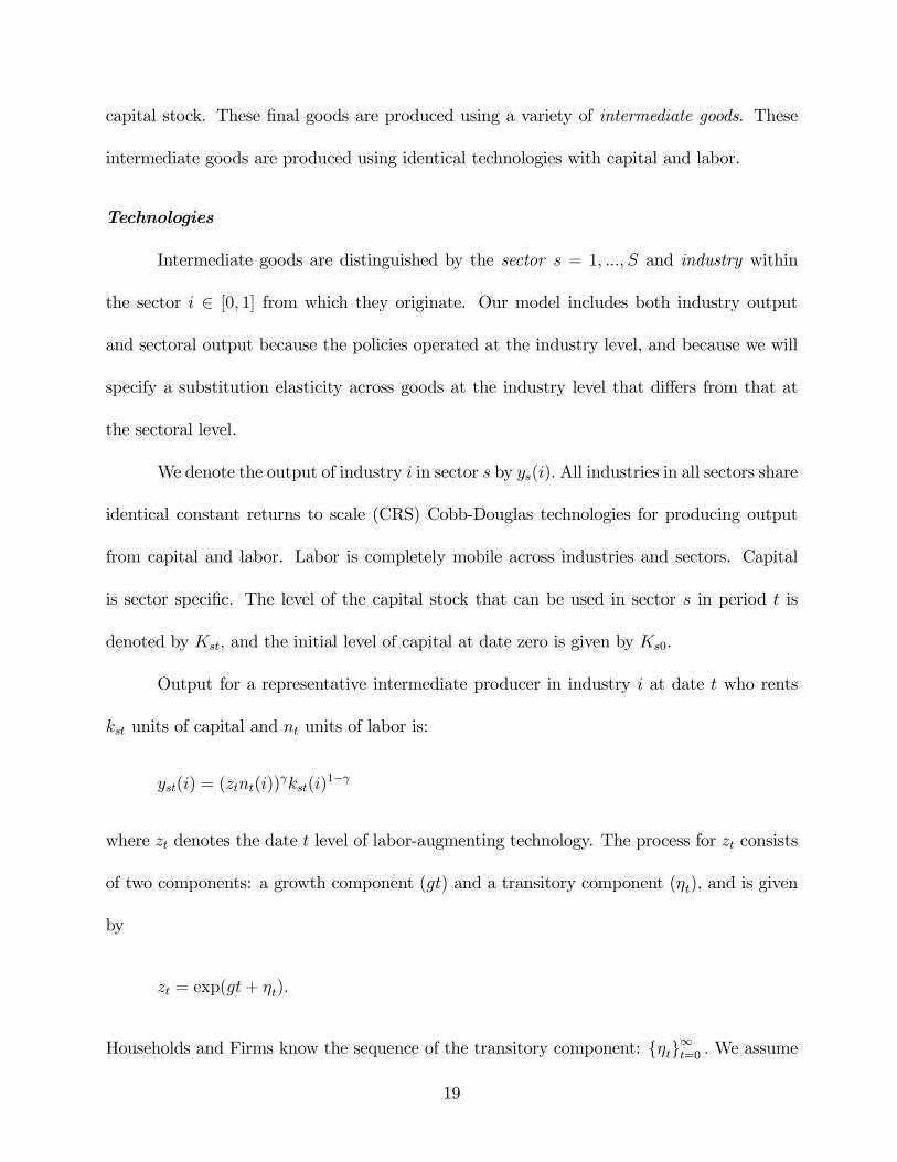
capital stock. These final goods are produced using a variety of intermediate goods. These

intermediate goods are produced using identical technologies with capital and labor.

Technologies

Intermediate goods are distinguished by the sector s = 1, ..., S and industry within

the sector i ∈ [0, 1] from which they originate. Our model includes both industry output

and sectoral output because the policies operated at the industry level, and because we will

specify a substitution elasticity across goods at the industry level that differs from that at

the sectoral level.

We denote the output of industry i in sector s by ys(i). All industries in all sectors share

identical constant returns to scale (CRS) Cobb-Douglas technologies for producing output

from capital and labor. Labor is completely mobile across industries and sectors. Capital

is sector specific. The level of the capital stock that can be used in sector s in period t is

denoted by Kst, and the initial level of capital at date zero is given by Ks0.

Output for a representative intermediate producer in industry i at date t who rents

kst units of capital and nt units of labor is:

yst(i) = (ztnt(i))γkst(i)

1−γ

where zt denotes the date t level of labor-augmenting technology. The process for zt consists

of two components: a growth component (gt) and a transitory component (ηt), and is given

by

zt = exp(gt+ ηt).

Households and Firms know the sequence of the transitory component: {ηt}∞t=0 . We assume

19

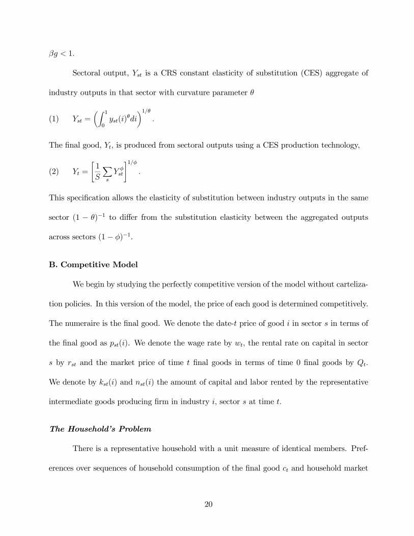
βg < 1.

Sectoral output, Yst is a CRS constant elasticity of substitution (CES) aggregate of

industry outputs in that sector with curvature parameter θ

Yst =µZ 1

0yst(i)

θdi¶1/θ

.(1)

The final good, Yt, is produced from sectoral outputs using a CES production technology,

Yt =

"1

S

Xs

Y φst

#1/φ.(2)

This specification allows the elasticity of substitution between industry outputs in the same

sector (1 − θ)−1 to differ from the substitution elasticity between the aggregated outputs

across sectors (1− φ)−1.

B. Competitive Model

We begin by studying the perfectly competitive version of the model without carteliza-

tion policies. In this version of the model, the price of each good is determined competitively.

The numeraire is the final good. We denote the date-t price of good i in sector s in terms of

the final good as pst(i). We denote the wage rate by wt, the rental rate on capital in sector

s by rst and the market price of time t final goods in terms of time 0 final goods by Qt.

We denote by kst(i) and nst(i) the amount of capital and labor rented by the representative

intermediate goods producing firm in industry i, sector s at time t.

The Household’s Problem

There is a representative household with a unit measure of identical members. Pref-

erences over sequences of household consumption of the final good ct and household market

20

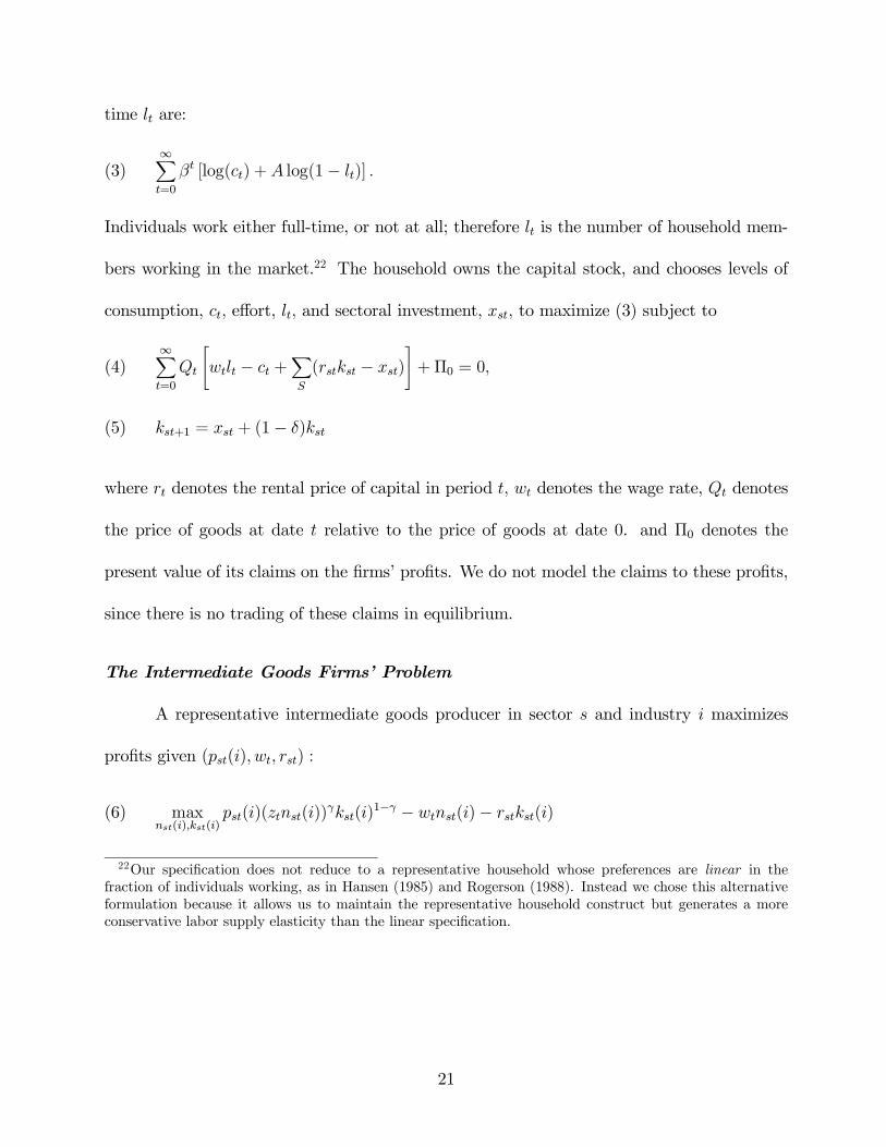
time lt are:

∞Xt=0

βt [log(ct) +A log(1− lt)] .(3)

Individuals work either full-time, or not at all; therefore lt is the number of household mem-

bers working in the market.22 The household owns the capital stock, and chooses levels of

consumption, ct, effort, lt, and sectoral investment, xst, to maximize (3) subject to

∞Xt=0

Qt

"wtlt − ct +

XS

(rstkst − xst)#+Π0 = 0,(4)

kst+1 = xst + (1− δ)kst(5)

where rt denotes the rental price of capital in period t, wt denotes the wage rate, Qt denotes

the price of goods at date t relative to the price of goods at date 0. and Π0 denotes the

present value of its claims on the firms’ profits. We do not model the claims to these profits,

since there is no trading of these claims in equilibrium.

The Intermediate Goods Firms’ Problem

A representative intermediate goods producer in sector s and industry i maximizes

profits given (pst(i), wt, rst) :

maxnst(i),kst(i)

pst(i)(ztnst(i))γkst(i)

1−γ − wtnst(i)− rstkst(i)(6)

22Our specification does not reduce to a representative household whose preferences are linear in thefraction of individuals working, as in Hansen (1985) and Rogerson (1988). Instead we chose this alternativeformulation because it allows us to maintain the representative household construct but generates a moreconservative labor supply elasticity than the linear specification.

21

The Final Good Firms’ Problem

A representative final goods producer, taking prices of its intermediate inputs as given,

{pst(i)}, also has a static profit maximization problem:

max

"1

S

Xs

µZ 1

0yds (i)

θdi¶φ/θ#1/φ

− 1

S

Xs

µZ 1

0ps(i)y

ds(i)di

¶(7)

where yds denotes the final good producer’s demand for the output from industry i in sector

s. This problem implies the following f.o.c.:

Y 1−φY φ−θs (yds(i))θ−1 − ps(i) = 0 for all i ∈ [0, 1] and s = 1, ..., S(8)

Market Clearing Conditions

The market clearing condition for labor is

lt =1

S

Xs

Z 1

0nst(i)di.

The market clearing condition for capital in sector s is

Kst ≥ 1

S

Z 1

0kst(i)di.

The market clearing condition for final goods is

Yt = Ct +Xt,

where Ct denotes aggregate consumption and Xt denotes aggregate investment.

Defining ydst(i) as the demand for output of firm i, the goods market clearing condition

for industry output is

ydst(i) = yst(i) for all s and i.

Note that the competitive version of this model is just a multi-sector version of the standard

optimal growth model.

22

C. The Cartel Model

We construct the cartel model by modifying the competitive model in two ways. First,

we allow a subset of industries to collude, and let the workers and firms in those industries

bargain over the wage and the number of workers. Second, the household’s time allocation

decision is modified so that household members may search for a scarce job in a cartelized

industry. This feature generates a dynamic insider-outsider model. While our cartel model

is in the spirit of other insider-outsider models, such as Blanchard and Summers (1986),

Lindbeck and Snower (1988), and Drazen and Gottfries (1994), the specific features of our

model differ from this earlier work. Modeling the main features of New Deal labor and

industrial policies requires a dynamic general equilibrium model in which employment and

the wage in the cartelized industries are determined in equilibrium as a function of the

bargaining strength of the workers and firms. The existing models in the literature do not

satisfy these requirements. Lindbeck and Snower’s model is static. Blanchard and Summers’

model imposes an exogenous employment rule that abstracts from modeling employment

changes. Drazen and Gottfries’ model assumes workers have all the bargaining power and

also uses a non-standard production technology. We now describe the cartel model.

The Household’s Problem

Household members either work in the competitive sector, (lft), work in the cartel

sector (lmt) (if the household member already has a cartel job), or search for a job in the

cartel sector (lut). It seems reasonable to assume that households will compete for the rents

from cartel jobs. In our model, households compete for these rents by searching for cartel

jobs. Searching, which consists of waiting for a vacant cartel job, requires the same amount

23

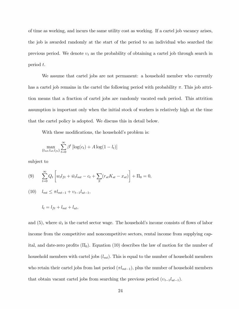
of time as working, and incurs the same utility cost as working. If a cartel job vacancy arises,

the job is awarded randomly at the start of the period to an individual who searched the

previous period. We denote υt as the probability of obtaining a cartel job through search in

period t.

We assume that cartel jobs are not permanent: a household member who currently

has a cartel job remains in the cartel the following period with probability π. This job attri-

tion means that a fraction of cartel jobs are randomly vacated each period. This attrition

assumption is important only when the initial stock of workers is relatively high at the time

that the cartel policy is adopted. We discuss this in detail below.

With these modifications, the household’s problem is:

max{lmt,lut,lft}

∞Xt=0

βt [log(ct) +A log(1− lt)]

subject to

∞Xt=0

Qt

"wtlft + wtlmt − ct +

XS

(rstKst − xst)#+Π0 = 0,(9)

lmt ≤ πlmt−1 + υt−1lut−1,(10)

lt = lft + lmt + lut,

and (5), where wt is the cartel sector wage. The household’s income consists of flows of labor

income from the competitive and noncompetitive sectors, rental income from supplying cap-

ital, and date-zero profits (Π0). Equation (10) describes the law of motion for the number of

household members with cartel jobs (lmt). This is equal to the number of household members

who retain their cartel jobs from last period (πlmt−1), plus the number of household members

that obtain vacant cartel jobs from searching the previous period (υt−1lut−1).

24

The Labor Market Clearing Conditions

In the cartel model, there are two separate labor markets: market clearing in the com-

petitive sector takes place through a competitive market, while cartel jobs are rationed and

workers search. Denoting labor employed by the competitive intermediate goods producers

by nft, the labor market clearing condition in the competitive sector is lft = (1 − m)nft.

Denoting labor employed in the cartel sector by nmt, the labor market clearing condition in

the cartel sector is lmt = mnmt. Finally, since those who search are randomly selected to join

the cartel sector, υt−1 = (nmt− πnmt−1)/lut−1. (The appendix discusses the determination of

the equilibrium level of υt in detail.)

The Negotiation Game

Our bargaining model is a two-stage negotiation game which is played each period in

each industry in a subset of the sectors in the economy. There are two players: workers and

firms. In stage one the workers make a wage and employment proposal: (wt, nt). The firms

either accept or reject this proposal. If the firms in the industry accept, they collude and

behave as a profit maximizing monopolist, subject to the constraint that they hire nt units

of labor at the wage wt.23 If the firms reject, they hire labor from the spot market at the spot

market wage, wt. In this case, however, firms can collude and behave as a profit-maximizing

monopolist only with probability ω < 1. With probability 1− ω, firms behave competitively

and thus do not earn any monopoly profits.24

23The monopolist is constrained in hiring labor decision, but they can hire any amount of capital at themarket rental price rt.24An important assumption in our cartel model is no entry. It is worth noting that there were two important

factors present in the 1930s that impeded entry. First, tariffs were high. This increased the cost of importingsubstitutes for the cartelized goods. Second, wages were high. Williamson (1968) argues that this can alsobe an effective barrier to entry.

25

At the beginning of a period, cartelized firms hire any additional workers randomly

from the pool of searchers from last period. In equilibrium the probability of a searcher

finding a job is equal to the number of new jobs in the cartelized industries divided by the

number of searchers.25

Symmetry implies we can aggregate the cartelized sectors and also aggregate the com-

petitive sectors. This allows us to work with a two sector model with a cartel sector of size

m and a competitive sector of size 1−m. The output of the cartel sector is:

Ymt ≡·Z 1

0yθmt(i)di

¸1/θ.

The output of the competitive sector is:

Yft ≡·Z 1

0yθft(i)di

¸1/θ.

The problems of the final goods producers and those intermediate goods producers in the

competitive sectors are the same as in the purely competitive model.

The Cartel Problems

We now specify the maximization problems for the firms and workers in a cartelzied

industries. It is useful to first define the profit function as a function of the wage rate

for monopolist in one of the cartelized sectors. We denote the monopolist’s profit function

conditional on the wage w, by Πt(w),and the associated optimal employment function by

25If the pool of these searchers is not large enough to cover the number of new jobs, then firms hire additionalworkers randomly from those who choose to work in the current period. If this occurred then there could bean additional gain from choosing to work, which, in equilibrium, was too small to induce search. This canarise because search is a discrete choice and hence if the gain to being in the cartel sector was sufficientlysmall then no one would search in the prior period, even if he was assured of obtaining a cartel job in thecurrent period. We do not discuss this possible case further, since in our quantitative analyses the benefit tobeing in the cartel sector was either zero or large enough to induce to search.

26

Nt(w), where

Πt(w) = maxn,k

Y 1−φt Y φ−θmt ((ztn)

γk1−γ)θ

−rmtk − wn

,(11)

and Nt(w) = n.26 In a slight abuse of notation we will use Πt(w, n) as the solution to the

monopolist’s maximization problem, when he takes wages and employment as given, and

hires the optimal quantity of capital.

We construct the sub-game perfect Nash equilibrium of this game that emerges as the

limit of our bargaining game played a finite number of periods within an individual industry.

In this case, the firm’s strategy in equilibrium is to always accept any wage and employment

offer (w, n) that yields a reservation level of profits. We then conjecture that the firms’

strategy in the infinitely repeated version of this game takes this form, and characterize the

solution to the workers’ decision problem. Finally we show our conjectured reservation profit

strategy for firms is a best response to the strategy that solves the workers’ problem.

First, consider the finite period game. Assume that in an individual industry the

workers and firms bargain for T periods, and that following period T workers and firms

behaved competitively. Since profits under competition are zero, the firms’ expected profits

from rejecting the workers’ offer, which we denote as PT , equals the probability of behaving

as a monopolist, ω, multiplied by monopoly profits, ωΠT (wT ), where wT denotes the date T

spot market wage in the competitive sector. Thus, the firms’ sub-game perfect strategy is to

accept any offer which yields profits of at least PT . This implies that the workers’ propose a

wage-employment offer of (wT , nT ) in period T such that firms earn profits of no more than

26The functions for Πt and Nt also depend upon Y, Ym and rt, but that is captured by the time dependenceof the functions.

27

PT . Now consider period T−1. Firms have the same reservation profit strategy in period T−1,

since equilibrium period T profits are independent of their period T − 1 actions. Continuing

backwards in this fashion implies that the firms’ strategy will be to accept any offer in period

t ≤ T that enables them to earn profits of at least Pt, where

Pt = ωΠt(wt).27(12)

The Workers’ Problem

The existing cartel workers’ objective is to offer a wage/employment pair at each date

that maximizes the present discounted value of rents from the cartelized sector.31 This value

depends on the existing stock of workers in the industry at the beginning of the period. We

denote the existing number of workers in the industry at the beginning of the period by n,

and we denote the number of those who actually work in the cartel that period by n. If n < n,

then n− n of the workers are randomly chosen to leave the industry. Given Pt, the solution

to the cartel workers’ problem is implicitly determined by the following Bellman equation in

which Vt(n) denotes the expected value of being a cartel worker (relative to working in the

competitive sector) with n workers in the industry at the beginning of period t:

Vt(n) = max(w,n)

½µmin

·1,n

n

¸¶[wt − wt + π(Qt+1/Qt)Vt+1(πn)]

¾(13)

subject to Πt(w, n) ≥ Pt.

31We assume families are large enough to smooth out a family member’s employment risk, but are smallenough to work in only an arbitrarily small fraction of the industries. These assumptions imply that the familyis risk neutral with respect to the employment outcome of any individual family member. Moreover, thisimplies that the family does not internalize the aggregate consequences of their actions since the likelihoodof a family member obtaining a cartel job is independent of the actions of the industries in which familymembers work.

28

This problem accounts for worker attrition in two ways. First, the stock of workers in the

industry at the beginning of next period will be πn. Second, an individual worker discounts

future payoffs by the discount factor π(Qt+1/Qt), since the probability that the worker remains

in the cartel is π.

Note that workers face the constraint that their proposal of (w, n) must yield the firms

their reservation profit level of Pt,which in equilibrium is given by (12). We denote the pair

(w∗t , n∗t ) as the maximum possible wage and the associated level of employment that satisfies

the minimum profit constraint.

Definition 1. For each t, define w∗t = Π−1t (Pt) and n∗t = Nt(w

∗t )

Note that since Π0t < 0, limw→∞Πt(w) = 0, and Pt ≤ Πt(wt) (monopoly profits at the

competitive wage), w∗t is well defined, and the value of Vt(n) defined in (13) is bounded above

byP∞τ=t π

τ−tQτ (w∗τ − wτ )/Qt. We assume that this bound is finite in each period.

Proposition 1. In problem (13), the optimal policy is such that

(i) Πt(w, n) = Pt

(ii) if n ≤ n∗t , then n ≥ n.

(iii) if n∗t < n ≤ Nt(wt) then nt = n.

(iv) if n > Nt(wt), then n ≤ n.

Proof. See the Technical Appendix.

Proposition 1 implies that workers always set their offer so that firms earn their reser-

vation profits. Moreover, if the initial stock of workers is above n∗t , no new workers are added,

and industry employment decays at the attrition rate of 1 − π until it reaches n∗t . It is this

29

case with relatively high employment that attrition plays a role. Without attrition, employ-

ment would remain permanently at that high level. Alternatively, if employment is below n∗t ,

employment is weakly increasing. We strengthen these results below by showing that if the

rest of the economy converges to a balanced growth path, then cartel employment converges

to n∗t .

The Firms’ Problem

Here we verify our conjecture that given workers’ strategy, the firms’ optimal strategy

is to accept any offer (wt, nt) that yields profits of at least ωΠt(wt). To do so, conjecture that

the continuation payoff to the firms from period t+ 1 onwards is given by

Wt+1 =∞X

τ=t+1

ÃQτQt+1

ωΠτ (wτ )

!.(14)

Note that this payoff is independent of the number of workers in the industry at the beginning

of period t+1. Next, consider what happens if firms reject the workers’ offer. With probability

ω they behave as a monopolist hiring labor at the competitive wage wt. In this case their

payoff is Πt(wt)+(Qt+1/Qt)Wt+1. If they reject the workers’ offer, then with probability 1−ω

each individual firm behaves competitively and a firm’s payoff is 0 + (Qt+1/Qt)Wt+1. Thus,

the expected payoff from rejecting the workers’ offer is ωΠt(wt) + (Qt+1/Qt)Wt+1.

Since the firms’ payoff from accepting the workers offer is Πt(wt, nt)+ (Qt+1/Qt)Wt+1,

the optimal strategy of the firms is to accept an offer of (wt, nt) if Πt(wt, nt) ≥ ωΠt(wt) and

otherwise reject. Since the workers’ optimal strategy is to offer firms their reservation profit

level, then in equilibriumWt = ωΠt(wt)+ (Qt+1/Qt)Wt+1, which is the date t version of (14).

This verifies our conjecture for both the firms’ continuation payoff and their optimal strategy.

30

Equilibrium Outcomes

Under certain conditions, the workers can attain a payoff equal to the discounted value

of the maximum wage. These conditions are laid out in the following proposition.

Proposition 2. If Nt+1(w∗t+1) ≥ πn∗t for t ≥ 0 and N0(w∗0) ≥ nm,−1 then for all t

wt = w∗t = Π

−1t (Pt), where Pt = ωΠt(wt),(15)

and the employment level is given by

nt = Nt(wt).(16)

Proof. See the Technical Appendix.

Along any balanced growth path the number of workers in an industry remains con-

stant. Thus the conditions of proposition 2 are satisfied, and the wage rate in the cartelized

industries is given by (15) and the employment level by (16). It will turn out that in our

transition path analyses the conditions of proposition 2 will be satisfied. This is because we

set the initial stock of workers in our transition simulations to employment levels from 1933,

which are below the balanced growth path levels.

As long as the conditions of proposition 2 are satisfied, then in equilibrium the workers

need only specify the wage in their contract with the firms since specifying a wage of w∗t and

allowing the firms to choose both the quantity of employment and the quantity of capital to

rent will generate the desired level of employment, n∗t , and leave the firms at their reservation

profit level.32

32This result is consistent with the fact that between 1933-1939 both the NIRA codes and union contractsoften specified only the wage and not the employment level. When the initial level of employment is high

31

When the conditions of Proposition 2 are satisfied and (16) holds, it is easy to show

that

Pt = Y1−φY φ−θm ym(i)

θ(1− θ),

where we have made us of (8).

The effects of this cartelization policy on employment and the wage depend on the

relative bargaining power between workers and firms, and this bargaining power is determined

by the parameter ω, which is the probability that firms can reject an offer and still collude.

The appendix illustrates this when the economy is on a balanced growth path. For example,

when ω = 1, firms have all the bargaining power. In this case, P is equal to monopoly profits,

and the cartel chooses the employment level that would arise if the industries in m sectors

were acting as monopolists. For values of ω < 1, the workers have some bargaining power,

and the cartel arrangement depresses employment relative to the monopoly case. As ω → 0,

workers have all the bargaining power. In this case, employment converge to zero. Finally,

we show that for any given ω > 0, as θ → 1, and the industry’s market power disappears,

the cartel economy’s balanced growth path converges to that of the competitive economy.

To understand these results, note that there are two opposing forces affecting the

number of cartel workers. First, the per-worker profits that must be paid to the firm (Pt/nmt)

increases as nmt falls. This force tends to increase employment. On the other hand, revenue

per worker is maximized by setting employment to zero, and this effect tends to reduce

employment. Since the impact of Pt/nmt declines as Pt falls, the second effect dominates the

enough that the workers want to set nt > n∗t , then the workers need to specify both the wage and theemployment level to force the firms to their reservation profit level. This implication of our model is consistentwith the observation that in declining industries employment is typically part of the factors being bargainedover.

32

first effect, and consequently employment and output in this industry tend to zero as Pt → 0.

One remaining issue is monotonicity of transition paths to the balanced growth path.

While we have not proved that the equilibrium sequences in our model monotonically converge

, our model simulations suggest they do. Proposition 2 covers the case where employment

starts at or below the balanced growth path level (n∗t ). It shows that if employment starts at

or below n∗0 and the sequence n∗t decreases at a rate less than 1− π, the maximum wage and

minimum employment level are chosen in each period. Propositions 1(ii) and 1(iii) cover the

case when initial employment is above n∗0and convergence is sufficiently monotonic. Then the

employment level decays at least at the rate 1− π down to n∗t , where it remains thereafter.

This model of New Deal policy sets up a dynamic insider-outsider friction in our model

that has the potential to significantly depress employment. The quantitative importance of

the insider-outsider friction depends on the reservation value of the firm Pt, which in turn

depends on the probability ω. Decreases in ω lower Pt, and reduce employment by shifting

bargaining power to the workers.

There are two reasons why the cartel model depresses employment: because insiders

maximize per-member profits and because new workers are paid the same wage as the insiders.

As we previously noted, this equal treatment characteristic was also a feature of New Deal

policies and wage agreements during the 1930s. We now turn to choosing parameter values

for the model.

5. Choosing Parameter Values

Many of the parameters of our model also appear in standard equilibrium business

cycle models. We choose values for these common parameters using the same methodological

33

approach used in the business cycle literature. The parameters ω, m,and π, however, are

specific to our model. Our general approach for these non-standard parameters is to either

use conservative values, or experiment and report results across a range of values.

The parameters that are common to other general equilibrium business cycle models

are γ, β, g, A, δ. We choose values for the first three of these parameters so that in the

competitive version of the model, along a balanced growth path, labor’s share of income is

70%, the annual real return to capital is 5%, and the growth rate of per-capita output is 1.9%

per year. We set the leisure parameter A so that households work about 1/3 of their time in

the competitive balanced growth path. We set δ = 0.07, which yields a balanced-growth-path

ratio of capital to output of 2.

There are two parameters that govern substitution elasticities between intermediate

goods: θ and φ. The parameter θ governs the elasticity of substitution between goods across

industries within a sector. This substitution parameter also appears in business cycle models

in which there is imperfect competition. In these models, the substitution parameter governs

the mark-up over marginal cost as well as the elasticity of substitution. In this imperfect

competition literature, a mark-up of about 10 percent over marginal cost is typically chosen.

We therefore choose θ = 0.9, which is consistent with this mark-up in a version of our model

with monopoly, but no labor market distortions.

The parameter φ governs the substitution elasticity between goods across the ag-

gregated cartelized and non-cartelized sectors. Since we are treating manufacturing as a

cartelized sector, we use long-run manufacturing data to determine a range of values for this

parameter. The relative price and expenditure share of manufactured goods have both de-

clined in the postwar period. These two trends are consistent with a substitution elasticity

34

between manufactured goods and other goods that is less than one. Thus, we consider a unit

substitution elasticity (φ = 0) as an upper bound on this parameter, and we also consider

substitution elasticities of 1/2 (φ = −1) and 1/3 (φ = −2). We found that the results were

insensitive to these different values for φ.

There are three parameters that are specific to our cartel model: m, ω and π. The first

parameter is the fraction of industries in the model economy that are cartelized. The second

parameter is the probability that a firm in a cartelized industry can act as a monopolist but

pay the non-cartel (competitive) wage. The third parameter is the cartel attrition rate, which

is the probability that a current cartel worker will remain in the cartel the following period.

We conduct the balanced growth path analysis for two values of the parameterm: 0.25

and 0.50. The first value is slightly smaller than manufacturing’s share of the economy in

1929. We view this as a conservative value for the cartelized fraction of the economy.33 The

second number is a little less than the share of total employment covered by the NIRA. After

analyzing the effects of these different values of m on the balanced growth path equilibrium,

we will choose a single value for this parameter for the transition path analysis.

The parameter ω is the probability that an industry fails to reach an agreement with

labor but still behaves as a monopolist. For the NIRA, this probability corresponds to the

likelihood that a firm in an effectively cartelized sector could have violated the contractual

labor provisions in their industry code. We conduct the balanced growth path analysis for a

range of values for this probability: .05, .50, 1. Recall that ω = 1 is a model in which labor has

33Hawley’s view (private communication) is that this number is a conservative estimate of the fraction ofthe economy that was effectively cartelized during the NIRA. The number is also conservative given the viewthat these policies were responsible for raising the manufacturing real wage. Manufacturing accounted forabout 28 percent of output in 1929.

35

no bargaining power, and the industries in fraction m of the sectors behave as monopolists.

We call this version of our model the monopoly model. As with the case of the parameter

m,we will choose a single value for this probability for the transition path analysis following

the balanced growth path analysis..

The parameter π is the probability that a cartel worker remains in the cartelized sector.

This parameter tries to capture naturally occurring job separations such as retirement and

disability due to accidents and illness. We choose π = 0.95, which corresponds to an expected

job tenure for a cartel worker of 20 years. We experimented by conducting our analyses for

two different values of this parameter which yield average job durations of 10 years and 40

years, respectively. We found that most of the results were not sensitive to these variations.

We now turn to the comparison of the cartel and competitive balanced growth paths.

6. Quantitative Analysis

A. Comparing the Cartel and Competitive Balanced Growth Paths

This section compares the balanced growth paths of the cartel version of the model, in

which fraction m of the sectors are cartelized, to that of the purely competitive model. Table

10 presents for the cartel model aggregate output (y), aggregate employment (n), the cartel

(insider) wage (wn), and employment (nm) in the cartel sector divided by their respective

balanced growth path values in the purely competitive economy. The table also presents the

fraction of workers searching for a job in the cartelized sector (s)

The main result is that the cartelization policy depresses aggregate output and employ-

ment if labor has a lot of bargaining power. This is the case when the parameter ω is low. For

example, with m = 0.25 and ω = 0.05, output falls 14 percent relative to pure competition.

36

For m = 0.50 and ω = 0.05, output falls about 25 percent relative to pure competition. The

reason that employment and output are so low in these two cases is because the insiders are

able to raise their wages substantially - the wage in the cartelized sector is about 36 percent

above its value in the purely competitive economy for the case of m = 0.25 and ω = 0.05.

The results also show that monopoly per se is not the key depressing factor, but rather it is

the link between wage bargaining and monopoly that raises wages above competitive levels.

In particular, the cartelized wage in the monopoly version of the model (ω = 1) is about the

same as the wage in the purely competitive model, and aggregate output and employment in

the monopoly model are close to their competitive levels. Thus, the cartelization policy is not

very depressing if firms have most of the bargaining power. This is because firms maximize

total monopoly profits, while insiders maximize only their own payoffs.

The results from Table 10 also show that the impact of the cartelization policy depends

on the fraction of the economy covered by these policies (m). Fixing the value for the

parameter ω and increasing m leads to larger decreases in aggregate output and employment,

and a relatively smaller increase in the cartelized wage.

The cartel policy also depresses employment in the competitive sector. This is due

to two factors: the complementarity factor and the rent-seeking factor. The complementar-

ity factor reduces employment in the competitive sector by reducing the competitive wage

through lower output from the cartelized sector. The rent-seeking factor reduces employment

in the competitive sector by inducing household members to compete for rents from cartelized

jobs. For example, for m = 0.25, ω = 0.05 about 5 percent of those individuals involved in

market activity search for a cartel job. For m = 0.5, ω = 0.05, about 11 percent of workers

search for a cartel job.

37

Before conducting the transition path analysis, we need to settle on values for m

and ω. We choose m = 0.32. This value is consistent with two procedures of estimating m.

The first is to measure m based on the fraction of the economy that appears to be effectively

carterlized - those sectors that experienced significant increases in wages and prices during the

recovery period. Manufacturing and mining are two such sectors. We earlier presented data

showing significant increases in wages and prices in both of these sectors, and also summarized

arguments made by Hawley and the FTC that industries in these sectors were behaving

collusively. Treating these two sectors as the only cartelized sectors yields m = 0.32.34 The

second approach to measuring m is based on the view that post-NIRA cartelization was

facilitated by trade unions that bargained with firms over wages. The share of unionized

private employment in 1939 also implies m = 0.32.35

This value of m may be viewed as a conservative one, since our analysis abstracts from

other cartelization policies of the 1930s. Other policies that may have restricted employment

and output include The Agricultural Adjustment Act, which was enacted to raise farm prices.

This act covered much of the farm sector, which accounts for about 30 percent of employ-

ment in 1929. Other examples of these policies include The Davis-Bacon Act, which required

federally-funded contractors to pay prevailing (union scale) wages and benefits, and the Fair

Labor Standards Act, which established a minimum wage, overtime pay, and restricted em-

ployment of workers under 18 years of age. Accounting for the effects of these policies could

raise the value of m.

Given m, the parameter ω pins down the cartelized wage along the balanced growth

34Manufacturing accounts for 28 percent of output, and mining accounts for 4 percent of output in 1929.35This number is the ratio of union workers to total private employment. Nonagricultural employment is

from the Historical Statistics of the United States, and agricultural employment is from Kendrick (1961).

38

path. We choose ω based on our estimate that the real wage in manufacturing is 20 percent

above its trend value during the recovery period. We therefore choose ω = 0.10, which

produces a balanced growth path wage in the cartel sector that is 20 percent above the

balanced growth path wage in the perfectly competitive version of the model.

B. Comparing the Equilibrium Paths in the Two Models to the Data: 1934-1939

This section presents the equilibrium paths for the purely competitive version and the

cartel version of our model from initial conditions in 1934 to their respective balanced growth

paths. We then compare the predicted variables from the two models between 1934 and 1939

to the data for those same years. For the cartel model, the cartelization policy is adopted in

1934.

Computing the equilibrium paths requires values for the initial conditions and a time

path for total factor productivity. The competitive model has one initial condition (capital

stock) and the cartel model has two initial conditions (capital stock and the number of

insiders in the cartelized sector). We find that the capital stock in 1934 is about 15 percent

below trend. We therefore specify the initial capital stock in each of the two sectors to be 15

percent below the balanced growth path level in the competitive model. We use the number

of workers in the manufacturing sector as the initial stock of insiders in the cartelized sector

in the cartel model. The stock of workers in manufacturing was about 42 percent below its

1929 level. In CO, we found that TFP in the data is significantly below trend in 1933, and

recovers back to trend by 1936. To account for the effects of this pattern, we feed in the

observed sequence of TFP values relative to trend between 1934-1936, and then feed in the

trend TFP value thereafter. The TFP numbers relative to trend for 1934-1936 are .926, .966

39

and .999, respectively.

With the initial capital stock in the two sectors and the sequence of TFP values, we

compute the perfect foresight transition path for the competitive and cartel versions of our

model. This is done by choosing a terminal date in the future such that the model is on its

respective balanced growth path, and then solving a system of N nonlinear equations in N

unknowns between the initial date (1934) and the terminal date.

We first consider the competitive model. Table 11 presents the transition path of the

competitive economy. Our main finding is that the predicted recovery from the competitive

model differs significantly from the actual 1934-39 recovery summarized in Table 1. Predicted

economic activity is too high, and the predicted wage is much lower than the wage in manu-

facturing. In particular, predicted output and labor input are both around their trend levels

by 1936, while actual output and labor input remain about 25 percent below trend. Predicted

consumption recovers nearly to trend by the end of the decade, while actual consumption

remains flat about 25 percent below trend. There is a very large disparity between predicted

and actual investment. Predicted investment recovers very quickly, and is 18 percent above

trend by 1936. In contrast, investment recovers only to 50% of its trend level. The predicted

wage is initially low, and then rises nearly to trend as TFP rises and the capital stock grows.

In contrast, the manufacturing wage is considerably above trend over the 1934-1939 period.

In summary, the predicted equilibrium path from the competitive model, which features a

very strong recovery with a low real wage, differs considerably from the actual path of the

U.S. economy between 1934 and 1939.

We now turn to the cartel model. Table 12 shows output, consumption, investment,

employment, searchers divided by the sum of workers and searchers (S), employment in the

40

cartel sector (nm), employment in the competitive sector (nf ), the wage in the cartel sector

(wm) and the wage in the competitive sector (wf ). The equilibrium path of the cartel model

is similar to the actual path of the economy between 1934 and 1939. We find that the cartel

model sheds light on the four major recovery anomalies identified in Section 2.

The first two anomalies are the weak recoveries in output and labor input. Actual labor

input and output rise from their trough levels between 1934-1936 and are then relatively flat

afterwards, remaining about 20-25 percent below trend. The cartel model predicts similar

patterns for these variables. Predicted output and labor input also rise between 1934 and

1936, and are flat afterwards. Predicted output in the cartel model is 14 percent below its

competitive balanced growth path level by 1939, while predicted employment is about 11

percent below its competitive balanced growth path level. Thus, the cartel model accounts

for about 50-60 percent of the post-1933 depression in output and labor input.

There are two reasons why the model predicts labor input and output rise during the

first two years of recovery. The first reason is that the initial stock of workers in the cartelized

sector in the model is below its steady state cartel level. Since in equilibrium the workers pay

the firm its reservation value, it is optimal for the small number of incumbent workers to add

new members and expand employment and output. The second reason is that productivity

increases, rising about 8 percent between 1934 and 1936. This increases the firm’s reservation

profit level in 1935 and 1936, which in turn leads the cartel to add additional workers.

The third recovery anomaly is consumption, which in the data is roughly flat through-

out the recovery, remaining about 25 percent below trend. The predicted pattern of consump-

tion in the cartel model is also flat, rising from 16 percent below its competitive balanced

growth path level in 1934 to 14 percent below in 1939. The model thus accounts for the flat

41

pattern in consumption and also accounts for over 50 percent of the post-1933 depression in

consumption.

The fourth recovery anomaly is investment, which in the data rises from 72 percent

below trend in 1933 to about 50 percent below trend in 1939. The cartel model predicts a

much stronger investment recovery - an increase from about 60 percent below its competitive

balanced growth path level in 1934 to 13 percent below in 1939. In subsection D, we return

to the deviation between predicted and actual investment, and discuss one modification to

the cartel model that brings predicted investment much closer to the data.

We now turn to discussing some other features of the data and the corresponding

predictions of the model.

The manufacturing wage, which we identify as a cartelized wage in the data, rises from

11 percent above trend in 1934 to about 20 percent above trend at the end of the decade.

The cartelized wage in the model exhibits a similar pattern. It rises from about 15 percent

above its competitive balanced growth path level in 1934 to 20 percent by 1939. While the

parameter ω was chosen so that the balanced growth path wage is 20 percent above the

competitive balanced growth path level, this choice places no restrictions on the time path

of the cartelized wage as it converges to its balanced growth path value. Thus, the model

qualitatively reproduces the time path in the cartel wage over the recovery period. The wage

in the competitive sectors of our cartel model is significantly below its competitive balanced

growth path level, despite normal productivity growth. It is 20 percent below its competitive

balanced growth path level in 1934, and remains 17 percent below in 1939. Unfortunately

there is no corresponding wage measure in the data for comparison.

The adoption of the cartel policy in our model generates monopoly rents. It is hard

42

to find profit measures in the data to compare to these theoretical monopoly rents, but it is

worth pointing out that manufacturing accounting profits rose significantly after the NIRA

was adopted, and rose faster than profits in other sectors. Moreover, industrial stock prices

also rose in 1934. This is also consistent with our model.

Our model predicts the fraction of individuals in the market sector who search for a

job. The number of searchers in our model, divided by the number who are either working

or searching, is 11 percent during the early part of the transition, and then declines to

about five percent. The unemployment rate is one empirical measure of the fraction of

individuals searching. Measured unemployment fluctuated between 16 percent in 1934 to

about 11 percent in 1939.36

Our model also makes different predictions about the cartelized and non-cartelized

sectors. In particular, the model predicts that employment and output in the cartelized

sectors falls more than labor input in the non-cartelized sectors. It is difficult to compare

this prediction to the data because it is hard to identify which sectors in the actual economy

were the non-cartelized sectors. Identifying the non-cartelized sectors is further complicated

by the adoption of other policies we abstract from that likely reduced competition in non-

manufacturing sectors, such as the Bacon-Davis Act and the Robinson-Patman Act. Given

36The search rate in our model depends on 3 features: the attrition rate, π, the representative familyconstruct, and the cost of searching, which we assume is equal to the cost of work. Randall Wright pointedout that search may be less costly than working, which would raise the fraction of household members whowere engaged in search.We have also conducted our analysis without job-search in the cartel sector. The results did not change

significantly. This is because ω determines the wage premium in the cartel sector, which in turn determinesrelative output and employment. Since the contribution of search to the overall level of effort is small,the disutility of working is only slightly effected by dropping costly search, and hence the levels of outputand employment are only marginally higher. For example, in the steady of state of the cartel model thatcorresponds to our transition examples; that is, when (m = .32,ω = 0.1,φ = −1), output is 88% of thecompetitive level instead of 86%, employment is 90% of the competitive level instead of 89%, however thecartel wage is about 20 percent above the competitive wage in both cases.

43

these limitations, we make a comparison between the manufacturing and mining sectors

and the non-farm economy. We chose this comparison because of data availability and our

assumption that manufacturing and mining were significantly affected by these policies. We

compare labor input data for these sectors from both Kendrick and Historical Statistics. Both

sources indicate that manufacturing and mining labor input were somewhat lower in the mid

and late 1930s than total non-farm labor input. Kendrick’s data shows that the average of

manufacturing and mining hours between 1934-39 is about 26 percent below its 1929 value,

and shows the average value for private non-farm hours (which includes these two sectors) is

about 18 percent below its 1929 value. The Historical Statistics data shows that the average

value for manufacturing and mining employment between 1934-39 is about 10 percent below

the 1929 value, while total non-farm employment is about 5 percent below its 1929 value.

Our model also predicts that the relative price of cartelized goods should rise. This

comparison is also difficult to make for the same reasons as above. We therefore compare

the price of investment goods to consumption goods. We also chose this comparison because

of data availability and because of our assumption that the investment goods sector (man-

ufacturing) was cartelized by these policies. Table 5 shows that the relative price of fixed

investment goods rose about 20 percent during the recovery period, and also shows that our

constructed measure of the relative price of manufacturing rose about 20 percent.

We also used our model to compute the welfare cost of the cartel policy. We found that

a permanent 4.9 percent increase in consumption was required to raise the level of discounted

lifetime utility in the cartel transition to that in the competitive transition. This welfare

cost is large relative to the welfare costs of other government policies, such as capital income

taxation (Chari, Christiano, Kehoe (1994)).

44

We have also conducted some sensitivity analyses to assess the robustness of our re-

sults. First, we consider an alternative parameterization in which we assume only a fraction

of the manufacturing and mining sectors are effectively cartelized. Second, we consider an-

other parameterization in which capital goods are produced entirely by the cartelized sector.

Third, we allow for some degree of initial monopolization.

C. Extension 1: Not all of Manufacturing and Mining are Cartelized

Our analysis assumed that all of manufacturing and mining were cartelized, and we

chose a value for ω so that the cartelized wage was about 20 percent above trend. An

alternative interpretation of these data is that only a fraction of manufacturing and mining

were cartelized, but that the wage in those cartelized industries was high enough to generate

the observed rise in the aggregate manufacturing wage. As a robustness check, we lowered the

fraction of the manufacturing and mining sectors that were effectively cartelized, and chose

ω for this smaller fraction of the economy to maintain a 20 percent increase in the average

cartelized wage in our model.

In this extension, we assumed that 75 percent, rather than 100 percent, of manufac-

turing and mining are cartelized, and chose ω so that the average wage in the two aggregate

sectors remained 20 percent above the level under pure competition. We found very similar

results. Steady state aggregate output in our cartelized economy is 87 percent of its balanced

growth path level in the competitive economy. Similarly, employment is 89 percent of the

competitive level.

45

D. Extension 2: Capital Exclusively Produced by the Cartelized Sector

One explanation for the increase in the relative price of capital is that capital goods are

produced largely by industries (e.g. the manufacturing sector) that were effectively cartelized

in the 1930s. This modification has important implications for the predicted level of invest-

ment in our cartel model.37

We modify our analysis by assuming that capital goods are produced solely from the

cartelized sector. This modification changes two resource constraints:

Ym =Zydm(i)di+X,

Y = C.

The model is otherwise unchanged.

With investment produced solely from the sectoral outputs of industries i ∈ [0,m], we

need to recalibrate m to maintain the share of cartelized employment equal to .32. Table

13 shows the balanced growth path for this version of the cartelized economy relative to the

balance growth path of the purely competitive model.

This modification increases the distorting effects of the cartelization policy. For ex-

ample with ω = 0.75, the cartelized wage is 19% higher than under pure competition, the

policy reduces output about 20 percent relative to pure competition, and reduces investment

about 45 percent below pure competition. This modification of our model captures the in-

crease in the relative price of capital goods, and suggests that our benchmark model may

37Another possible explanation is that if capital was industry specific, then firms would have a reducedincentive to invest because of a holdup problem: increasing the capital stock would have lead the workers toraise their wage demands.

46

have understated the depressing effects of New Deal cartelization policies.

E. Extension 3: Introducing Some Monopoly in 1929

Our experiments assumed that the starting point of our analysis (1929) was pure

competition. An alternative view is that there was monopoly in some sectors of the U.S.

economy in 1929, and that the New Deal made it possible for more sectors to collude.

To model this alternative view, we modify our model by assuming there are sub-

industries producing a distinct good within an industry, and that the New Deal policies

allowed collections of producers within an industry to collude, whereas before the Depression

only those within a sub-industry had been able to collude.

We assume there a large number of sub-industries indexed by i on the unit interval,

and that there are a large number of industries within each sector, indexed by j on the unit

interval. The output of an industry j, which we denote by Yst(j) is given by

Yst(j) =µZ 1

0yjst(i)

θdi¶1/θ

,

where yjst(i) denotes the output of sub-industry i in industry j. The output of a sector is

given by

Yst =µZ 1

0Yst(j)

γdj¶1/γ

,

where the difference between γ and θ determines the additional degree of monopoly power

that an industry cartel enjoys relative to a sub-industry cartel.38

To make this operational, we assume that half as many sectors were behaving collu-

sively prior to 1929 as after 1933, and that the price elasticity they faced changed from -10

38Note the these changes do not change the aggregate production set. In particular, if yjst(i) = y, thenYst(j) = ym, and hence Yst = y.

47

to -9 (which implies that γ = .89). We retain m = .32, φ = −1,and ω = 0.10.

In this case output starts at 78% of it’s balanced growth path level under partial

monopoly (PM), and rises gradually to 88% of this level by 1939. Consumption is fairly flat,

starting out at 85% of it’s PM level, and rising gradually to 87% by 1939. Investment is

quite depressed, starting out at 47% of PM, but then it rises rapidly to 91% of PM by 1939.

Employment is also depressed, but by less than output, starting out at 86% of PM and then

rising to 92% of PM by 1939. The wage premium starts at 13% above it’s PM level in 1934

and rises to 20% above PM by 1939.39

These results indicate that the basic thrust of our results continue under this variant

of the model, though the impact is somewhat reduced. Of course, assuming the capital was

produced in the cartel sector would increase these effects.

7. Implications of Time Variation in New Deal Policies

For simplicity, our analysis abstracts from time variation in New Deal policies. This

section discusses two changes in these policies and the implications of these changes for our

analysis.

A. The Increase in Labor Bargaining Power and the Downturn of 1937-38

The first change we discuss is the relative increase in labor bargaining power in 1937.

The Supreme Court upheld the constitutionality of the NLRA in 1937. This increased union-

ization and the number of strikes substantially in 1937 and 1938. Moreover, State governments

permitted “sit-down” strikes, in which employees took over plants and halted production,

39In this computation we assumed that any initial difference among the cartelized sectors due to some ofthem behaving monopolistically and some behaving competitively was wiped out between 1929 and 1933.Hence we assume that all of the cartelized sectors have the same level of initial capital in 1934.

48

during this period. These changes in unionization and union activity led to significantly

higher wages; manufacturing real wages rose about nine percent between 1936 and 1938.

Our cartelization theory predicts that this increase in labor bargaining power should have

increased wages and reduced employment and output during this period. This prediction is

consistent with the fall in output, employment, and investment that occurred between 1937

and 1938.

This bargaining power explanation of the 1937-38 downturn differs from the standard

explanation, which is that the downturn was caused by higher reserve requirements on bank

accounts. CO (1999) note that it is difficult to explain the 1937-38 downturn solely by higher

reserve requirement. If this factor was the sole cause, commercial loan rates and the spread

between lending and borrowing rates should have increased shortly after these changes in

reserve requirements, and output should have begun to decrease shortly after these increases.

In contrast, commercial loan rates and the spread between loan rates and other rates were

roughly unchanged after these increases, and industrial production continued to grow for 14

months after the first and largest of these increases. While more work is required to assess

the 1937-38 downturn, our theory raises the possibility that an increase in labor bargaining

power may have been an important contributing factor to the downturn of 1937-38.

B. The Reversal of New Deal Policies and the Wartime Economic Boom

The second change we discuss is the dismantling of these policies during the 1940s

and the effect of this policy reversal on employment and output. The economy expanded

significantly during World War II. Our cartel model with permanent New Deal policies and

no other shocks, however, predicts that the economy should have remained depressed. This

49

section briefly discusses that the wartime expansion can be reconciled with our cartel model.

This is because the expansion coincided with a considerable increase in antitrust prosecution

and a significant weakening in labor’s bargaining power.

By the late 1930s Roosevelt suggested that cartelization may have been a contributing

factor to the persistence of the Depression. Roosevelt appointed Thurman Arnold to direct

the Antitrust Division of the DOJ. Under this new leadership, the number of new cases

brought by the DOJ rose from just 57 between 1935-39 to 223 between 1940-44. About 80

percent of these cases were won by the government.40

Labor policy also changed during the 1940s. First, The Supreme Court ruled in 1939

that the “sitdown strike” was unconstitutional. Labor historians view this decision as signifi-

cantly weakening labor’s bargaining power (See Kennedy). Second, collective bargaining was

largely suspended during the War as the National War Labor Board (NWLB) ruled on wage

increases, and largely granted only cost of living increases. Third, strikes by Coal miners dur-

ing the war pushed public opinion and congressional opinion against unions and the NLRA.

By 1947, as the NWLB was disbanded, the NLRA was amended by the Taft-Hartley Act.

This Act weakened labor’s bargaining power by restricting labor’s actions, and by reducing

the original limitations placed on firms in the original NLRA. Among other changes, the Act

outlawed the closed shop, and gave states the right to outlaw unions shops.

Our model predicts that variations in labor and industrial policies should have affected

the difference between the wage and productivity, and also affected the level of employment

and output. Table 14 shows that the manufacturing wage relative to manufacturing labor

40See Posner, R.A., “A Statistical Analysis of Antitrust Enforcement,” Journal of Law and Economics(October 1970) vol. 13, p. 365-420.

50

productivity changed between 1929 and 1950. It increased considerably during the Depression

years (1938 compared to 1929), and then decreased considerably during the expansion years

1950 relative to 1939. Our model predicts that this decline is consistent with the changes in

policies that occurred over this period.

While more work is needed to determine how these labor and industrial policy changes

affected macroeconomic activity duringWorldWar II, the significant change in wartime policy

indicates that our model may be consistent with the wartime economic boom.

8. Conclusion

The recovery from the Great Depression was weak despite rapid productivity growth,

and was accompanied by significant increases in real wages and prices in several sectors of

the economy. A successful theory of the recovery from the Depression should account for

persistent low levels of consumption, investment, and employment, the high real wage, and

the apparent lack of competition in the labor market. We developed a model with New Deal

labor and industrial policies that can account for sectoral high wages, a distorted labor market,

and depressed employment, consumption, and investment despite normal productivity.

Our results suggest that New Deal policies are an important contributing factor to

the persistence of the Great Depression. The key depressing element behind these policies

was not monopoly per se, but rather linking the ability of firms to collude with paying

high wages. Our model indicates that these policies reduced consumption, and investment

about 14 percent relative to their competitive balanced growth path levels. Thus, the model

accounts for about half of the continuation of the Great Depression between 1934 and 1939.

New Deal labor and industrial policies did not lift the economy out of the Depression

51

as President Roosevelt and his economic planners had hoped. Instead, the joint policies of

increasing labor’s bargaining power, and linking collusion with paying high wages, impeded

the recovery by creating an inefficient insider-outsider friction that raised wages significantly

and restricted employment. The recovery would have been stronger if wages in key sectors

had been lower.

52

References

[1] Alchian, A. Information Costs, Pricing, and Resource Unemployment, in Microeconomic

Foundations of Employment and Inflation Theory, E.S. Phelps, ed, Norton, NY 1970

[2] Beney, Ada Differentials in Industrial Wages and Hours in the United States, National

Industrial Conference Board, 1938.

[3] Bernanke, Ben Employment, Hours, and Earnings in the Depression: An Analysis of

Eight Manufacturing Industries, American Economic Review, March 1986, vol 76, num-

ber 1. 82-109.

[4] . 1995. The macroeconomics of the Great Depression: A comparative ap-

proach. Journal of Money, Credit, and Banking 27 (February): 1—28.

[5] Cole, H. and L. Ohanian. The Great Depression in the United States from a Neoclassical

Perspective, Federal Reserve Bank of Minneapolis Quarterly Review, (Winter 1999) vol.

23, no. 1, p. 25-31.

[6] Chari,V.V., Lawrence J. Christiano, and Patrick J.Kehoe, “Optimal Fiscal Policy in

a Business Cycle Model,” Journal of Political Economy, 102(4), August 1994, pages

617-52.

[7] Chari, V.V., P. Kehoe, and E. McGrattan. “Sticky Price Models of the Business Cycle:

Can the Contract Multiplier Sove the Persistence Problem,” Federal Reserve Bank of

Minneapolis Staff Report # 217.

[8] Dearing, Charles, Paul Homan, Lewis Lorwin, Leverett Lyon, The ABC of the NRA,

Wash DC, Brookings Inst. , 1934

53

[9] Friedman, Milton, and Anna Schwartz, A Monetary History of the United States, Prince-

ton, NJ, Princeton University Press. 1963

[10] Hanes, Christopher. 1996. Changes in the cyclical behavior of real wage rates, 1870-1990.

Journal of Economic History 56 (December): 837—61.

[11] Harbison, Federick. The Seniority Principal in Union-Management Relations, Industrial

Relations Section Report No. 57, Department of Economincs and Social Institutions,

Princeton University, 1939.

[12] Hawley, Ellis. The New Deal and the Problem of Monopoly, Princeton U Press, 1966.

[13] Historical Statistics of the United States, U.S. Dept of Commerce, part 1 and part 2.

[14] Ickes, H. The Secret Diaries of Harold Ickes, New York, Simon and Schuster

[15] Johnson, Hugh S. The Blue Eagle From Egg to Earth, Doubleday, Doran and Company,

Inc., Garden City, NY 1935

[16] Kendrick, John W. 1961. Productivity trends in the United States. Princeton, N.J.:

Princeton University Press.

[17] Kennedy, David M. Freedom From Fear: The United States, 1929-1945, Oxford History

of the United States, vol. 9, 1999.

[18] Lucas, R. and L. Rapping, Unemployment in the Great Depression: Is there a Full

Explanation? JPE, 1972, vol 80, no. 1, 186-191.

54

[19] Lyon, L., P. Homan, L. Lorwin, G. Terborgh, C. Dearing, L. Marshall. The National

Recovery Administration: An analysis and Appraisal, The Brooking Institution, Wash-

ington D.C., 1935.

[20] Mills, Harry and Emily Brown, From the Wagner Act to Taft-Hartley, The University

of Chicago Press, 1950.

[21] The National Recovery Administration, Report of the President’s Committee of Indus-

trial Analysis, U.S. Committee of Industrial Analysis, 1937, USGO

[22] Office of National Recovery Administration, Division of Review, - History of the Com-

pliance Division - by W.M. Galvin, J.J. Reinstein, D.Y. Campbell, Work Materials No.

85, March 1936

[23] Office of National Recovery Administration, Division of Review, - Legal Aspects of Labor

Problems - Minimum Wages, by Melvin Sims, Work Materials No. 43, Feb. 1936

[24] Posner, R.A., “A Statistical Analysis of Antitrust Enforcement,” Journal of Law and

Economics (October 1970) vol. 13, p. 365-420.

[25] Reynolds, Lloyd and Cynthia Taft. The Evolution of Wage Structure. Yale University

Press, New Haven, 1956.

[26] Romer, Christina. “Why Did Prices Rise in the 1930s?,” Journal of Economic History;

59(1), March 1999, pages 167-99.

[27] Ross, Arthur M. Trade Union Wage Policy, University of California Press, Berkely, CA,

1948.

55

[28] Taft, P. Organized Labor in American History - Harper and Row New York 1964

[29] US Gov printing Office- Codes of Fair Competition, nos. 1-.1933-34 - many volumes.

[30] Weinistein, Michael. Recovery and Redistribution Under the NIRA, North Holland Pub-

lishing Co., 1980.

56

9. Technical Appendix

This appendix describes details of the model, constructs the balanced growth path

equilibria, presents proofs of the propositions, and shows how the cartel model can be re-

interpreted as a model of a labor managed firm. We begin with the model details.

The households’ first order conditions include the following equations for optimal

choices of consumption, labor input in the competitive sector, investment, labor input in

the cartel sector, and search for a cartel job.

βt1

ct= Qtλ(17)

βtA

1− lt = λQtwt,(18)

Qt+1[rs,t+1 + 1− δ]−Qt = 0,(19)

Qtwtλ−Qtξt +Qt+1πξt+1 = βtA1

1− lt(20)

Qt+1υtξt+1 = βtA

1

1− lt ,(21)

where λ is the Lagrange multiplier on the budget constraint (9) and ξt is the Lagrangian

multiplier on the market hours constraint (10).

Cartel Job Acquisition

Since there is perfect insurance within the household, (18) and (19) can be used to

solve for the equilibrium probability of receiving a cartel job from searching. Assuming that

limτ→∞Qt+τπτξt+τ/Qt = 0, the value of being a cartel worker is

ξt =λ

Qt

∞Xτ=0

Qt+τπτ (wt+τ − wt+τ ).

57

Thus, the value to a household member of being in the cartel is the expected discounted value

of the cartel wage premium. Combining this expression with the time cost of searching for a

cartel job from (20) yields

υt−1∞Xτ=0

Qt+τπτ (wt+τ − wt+τ ) = Qt−1wt−1.(22)

This condition determines the equilibrium probability of finding a cartel job.

A. The Balanced Growth Paths

We first characterize the balanced growth path of the competitive model. We then

characterize the balanced growth path of the cartel model.

The Competitive model:

Conjecture that along the balanced growth path growth path the variables (ct, xt, Yt, Yst, yst(i), wt)

grow at rate g and that the variables (nt, rt, pst(i)) are constant. We will now verify this conjec-

ture. To do so, we denote (ct, xt, Yt, Yst, yst(i), wt) by their detrended level (c, x, y, ys, ys(i), w)

(that is, ct = cgt) and (nt, rt, pit) by their time-invariant levels (n, r, pi).

From the consumer’s f.o.c.s, we have

Qt =

Ãβ

g

!t(23)

w(1− n) = Ac(24)

Given the symmetry of the model, ouput in each industry in the two sectors is identical,

or ym(i) = yf(i), and therefore the price of each of these intermediate output in terms of

the final good is one, or ps(i) = 1. Moreover, since from symmetry all sectoral variables are

identical and the model essentially collapses to the one sector growth model, and we therefore

dispense with distinction between industries and sectors in much of what follows.

58

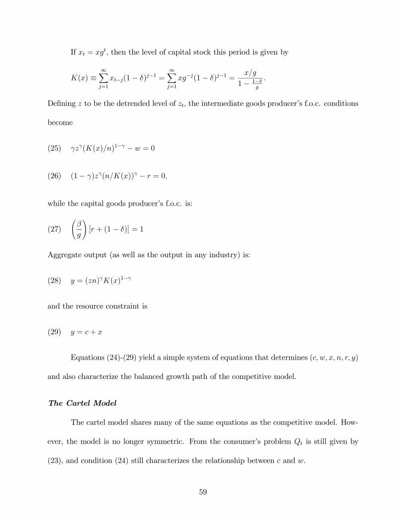
If xt = xgt, then the level of capital stock this period is given by

K(x) ≡∞Xj=1

xt−j(1− δ)j−1 =∞Xj=1

xg−j(1− δ)j−1 = x/g

1− 1−δg

.

Defining z to be the detrended level of zt, the intermediate goods producer’s f.o.c. conditions

become

γzγ(K(x)/n)1−γ − w = 0(25)

(1− γ)zγ(n/K(x))γ − r = 0,(26)

while the capital goods producer’s f.o.c. is:

Ãβ

g

![r + (1− δ)] = 1(27)

Aggregate output (as well as the output in any industry) is:

y = (zn)γK(x)1−γ(28)

and the resource constraint is

y = c+ x(29)

Equations (24)-(29) yield a simple system of equations that determines (c, w, x, n, r, y)

and also characterize the balanced growth path of the competitive model.

The Cartel Model

The cartel model shares many of the same equations as the competitive model. How-

ever, the model is no longer symmetric. From the consumer’s problem Qt is still given by

(23), and condition (24) still characterizes the relationship between c and w.

59

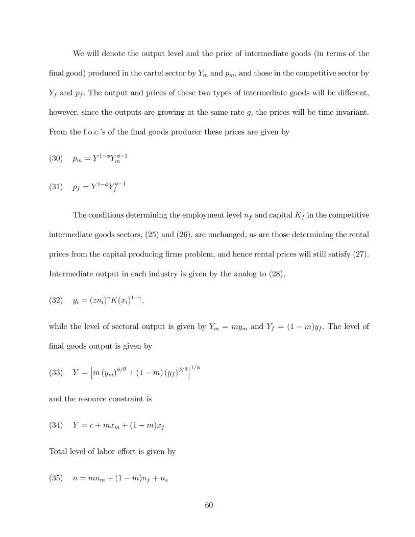
We will denote the output level and the price of intermediate goods (in terms of the

final good) produced in the cartel sector by Ym and pm, and those in the competitive sector by

Yf and pf . The output and prices of these two types of intermediate goods will be different,

however, since the outputs are growing at the same rate g, the prices will be time invariant.

From the f.o.c.’s of the final goods producer these prices are given by

pm = Y1−φY φ−1m(30)

pf = Y1−φY φ−1f(31)

The conditions determining the employment level nf and capitalKf in the competitive

intermediate goods sectors, (25) and (26), are unchanged, as are those determining the rental

prices from the capital producing firms problem, and hence rental prices will still satisfy (27).

Intermediate output in each industry is given by the analog to (28),

yi = (zni)γK(xi)

1−γ,(32)

while the level of sectoral output is given by Ym = mym and Yf = (1 −m)yf . The level of

final goods output is given by

Y =hm (ym)

φ/θ + (1−m) (yf)φ/θi1/φ

(33)

and the resource constraint is

Y = c+mxm + (1−m)xf .(34)

Total level of labor effort is given by

n = mnm + (1−m)nf + ns(35)

60

We now need to characterize the solution to the cartelized intermediate goods produc-

ers. We start first with the determination of P. It is easy to see from monopolist’s problem

(11) that from the associated f.o.c.s that the optimal choices by the monopolist for labor, n

and capital, k, will be such that

n

k=r

w

γ

1− γ .

This yields the following expression for k :

k =

"r

θpmY 1−θm (zrγ/w(1− γ))γ(θ−1) (1− γ)(zrγ/w(1− γ))γ# 1θ−1

This allows us to define the firm’s static expected payoff from turning down the workers’ offer

as:

P = ω½pmY

1−θm

³k(zrγ/w(1− γ))γ

´θ − rk − wk(rγ/w(1− γ))¾ .(36)

Since the balanced growth path level of employment in the cartel industries is constant at

nm, and nm > πnm, it follows that when condition (16) holds, nm satisfies

θpmγzγ(km/nm)

1−γ −Ãpm(znm)

γk1−γm − rkm − Pnm

!= 0.(37)

Since firms are acting as a monopolist and optimizing with respect to km, then the following

condition must hold

θpm(1− γ)(znm/km)γ − r = 0.(38)

The wage rate in the monopolist industry is given by

w =pm(znm)

γk1−γm − rkm − Pnm

(39)

61

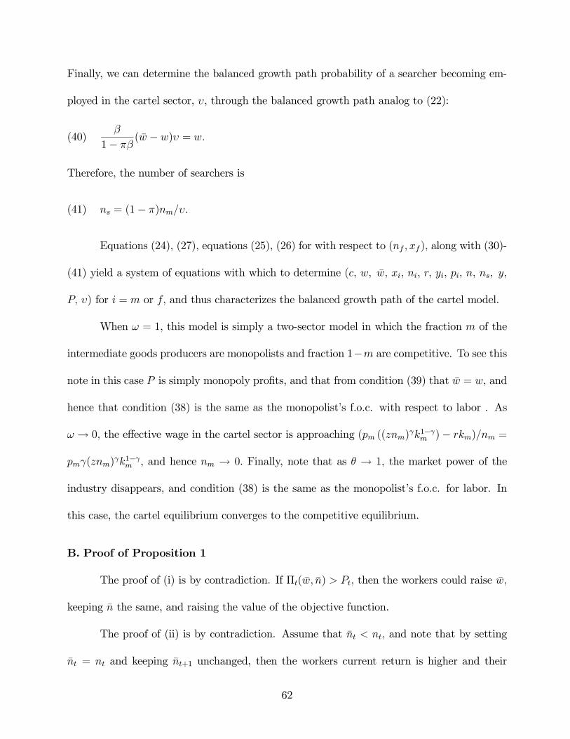
Finally, we can determine the balanced growth path probability of a searcher becoming em-

ployed in the cartel sector, υ, through the balanced growth path analog to (22):

β

1− πβ (w − w)υ = w.(40)

Therefore, the number of searchers is

ns = (1− π)nm/υ.(41)

Equations (24), (27), equations (25), (26) for with respect to (nf , xf ), along with (30)-

(41) yield a system of equations with which to determine (c, w, w, xi, ni, r, yi, pi, n, ns, y,

P, υ) for i = m or f, and thus characterizes the balanced growth path of the cartel model.

When ω = 1, this model is simply a two-sector model in which the fraction m of the

intermediate goods producers are monopolists and fraction 1−m are competitive. To see this

note in this case P is simply monopoly profits, and that from condition (39) that w = w, and

hence that condition (38) is the same as the monopolist’s f.o.c. with respect to labor . As

ω → 0, the effective wage in the cartel sector is approaching (pm ((znm)γk1−γm )− rkm)/nm =

pmγ(znm)γk1−γm , and hence nm → 0. Finally, note that as θ → 1, the market power of the

industry disappears, and condition (38) is the same as the monopolist’s f.o.c. for labor. In

this case, the cartel equilibrium converges to the competitive equilibrium.

B. Proof of Proposition 1

The proof of (i) is by contradiction. If Πt(w, n) > Pt, then the workers could raise w,

keeping n the same, and raising the value of the objective function.

The proof of (ii) is by contradiction. Assume that nt < nt, and note that by setting

nt = nt and keeping nt+1 unchanged, then the workers current return is higher and their

62

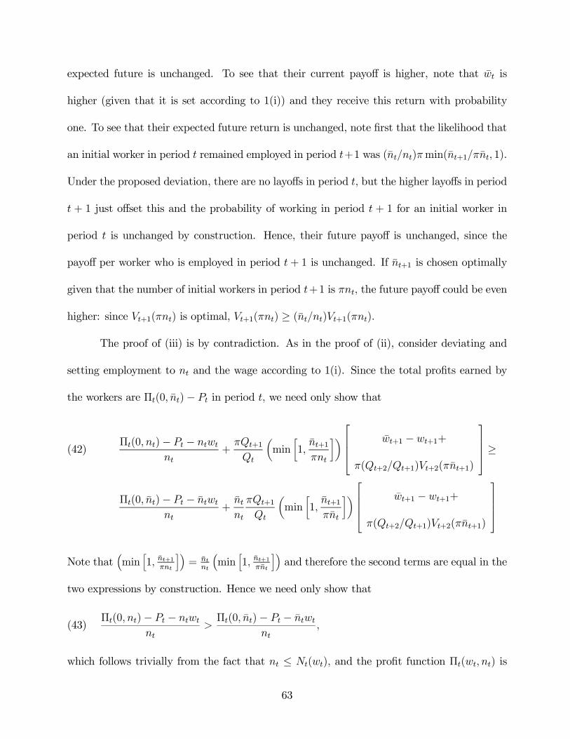
expected future is unchanged. To see that their current payoff is higher, note that wt is

higher (given that it is set according to 1(i)) and they receive this return with probability

one. To see that their expected future return is unchanged, note first that the likelihood that

an initial worker in period t remained employed in period t+1 was (nt/nt)πmin(nt+1/πnt, 1).

Under the proposed deviation, there are no layoffs in period t, but the higher layoffs in period

t + 1 just offset this and the probability of working in period t + 1 for an initial worker in

period t is unchanged by construction. Hence, their future payoff is unchanged, since the

payoff per worker who is employed in period t+ 1 is unchanged. If nt+1 is chosen optimally

given that the number of initial workers in period t+1 is πnt, the future payoff could be even

higher: since Vt+1(πnt) is optimal, Vt+1(πnt) ≥ (nt/nt)Vt+1(πnt).

The proof of (iii) is by contradiction. As in the proof of (ii), consider deviating and

setting employment to nt and the wage according to 1(i). Since the total profits earned by

the workers are Πt(0, nt)− Pt in period t, we need only show that

Πt(0, nt)− Pt − ntwtnt

+πQt+1Qt

µmin

·1,nt+1πnt

¸¶ wt+1 − wt+1+

π(Qt+2/Qt+1)Vt+2(πnt+1)

≥(42)

Πt(0, nt)− Pt − ntwtnt

+ntnt

πQt+1Qt

µmin

·1,nt+1πnt

¸¶ wt+1 − wt+1+

π(Qt+2/Qt+1)Vt+2(πnt+1)

Note that³min

h1, nt+1

πnt

i´= nt

nt

³min

h1, nt+1

πnt

i´and therefore the second terms are equal in the

two expressions by construction. Hence we need only show that

Πt(0, nt)− Pt − ntwtnt

>Πt(0, nt)− Pt − ntwt

nt,(43)

which follows trivially from the fact that nt ≤ Nt(wt), and the profit function Πt(wt, nt) is

63

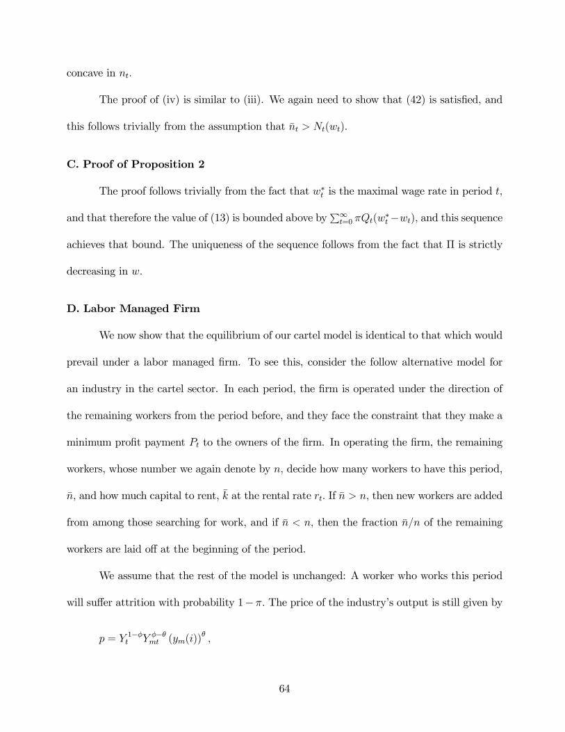
concave in nt.

The proof of (iv) is similar to (iii). We again need to show that (42) is satisfied, and

this follows trivially from the assumption that nt > Nt(wt).

C. Proof of Proposition 2

The proof follows trivially from the fact that w∗t is the maximal wage rate in period t,

and that therefore the value of (13) is bounded above byP∞t=0 πQt(w

∗t −wt), and this sequence

achieves that bound. The uniqueness of the sequence follows from the fact that Π is strictly

decreasing in w.

D. Labor Managed Firm

We now show that the equilibrium of our cartel model is identical to that which would

prevail under a labor managed firm. To see this, consider the follow alternative model for

an industry in the cartel sector. In each period, the firm is operated under the direction of

the remaining workers from the period before, and they face the constraint that they make a

minimum profit payment Pt to the owners of the firm. In operating the firm, the remaining

workers, whose number we again denote by n, decide how many workers to have this period,

n, and how much capital to rent, k at the rental rate rt. If n > n, then new workers are added

from among those searching for work, and if n < n, then the fraction n/n of the remaining

workers are laid off at the beginning of the period.

We assume that the rest of the model is unchanged: A worker who works this period

will suffer attrition with probability 1−π. The price of the industry’s output is still given by

p = Y 1−φt Y φ−θmt (ym(i))θ ,

64

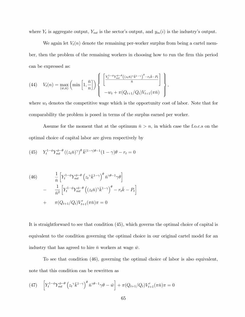
where Yt is aggregate output, Ymt is the sector’s output, and ym(i) is the industry’s output.

We again let Vt(n) denote the remaining per-worker surplus from being a cartel mem-

ber, then the problem of the remaining workers in choosing how to run the firm this period

can be expressed as:

Vt(n) = max(w,n)

µmin

·1,n

n

¸¶

"Y 1−φt Y φ−θmt ((ztn)γ k1−γ)

θ−rtk−Ptn

#

−wt + π(Qt+1/Qt)Vt+1(πn)

,(44)

where wt denotes the competitive wage which is the opportunity cost of labor. Note that for

comparability the problem is posed in terms of the surplus earned per worker.

Assume for the moment that at the optimum n > n, in which case the f.o.c.s on the

optimal choice of capital labor are given respectively by

Y 1−φt Y φ−θmt ((ztn)γ)θ k(1−γ)θ−1(1− γ)θ − rt = 0(45)

1

n

·Y 1−φt Y φ−θmt

³ztγk1−γ

´θnγθ−1γθ

¸(46)

− 1

n2

·Y 1−φt Y φ−θmt

³(ztn)

γ k1−γ´θ − rtk − Pt¸

+ π(Qt+1/Qt)V0t+1(πn)π = 0

It is straightforward to see that condition (45), which governs the optimal choice of capital is

equivalent to the condition governing the optimal choice in our original cartel model for an

industry that has agreed to hire n workers at wage w.

To see that condition (46), governing the optimal choice of labor is also equivalent,

note that this condition can be rewritten as

·Y 1−φt Y φ−θmt

³ztγ k1−γ

´θnγθ−1γθ − w

¸+ π(Qt+1/Qt)V

0t+1(πn)π = 0(47)

65

once we note that w is implicitly given here by

w =

·Y 1−φt Y φ−θmt

³(ztn)

γk1−γ´θ − rtk − Pt¸

n.

The f.o.c.s on n and w in our the workers’ problem in our cartel problem (13), again

assuming that n ≥ n and making use of Π which was defined in (11), are respectively given

by

π(Qt+1/Qt)V0t+1(πn)π + λ

∂Πt(w, n)

∂n= 0(48)

1 + λ∂Πt(w, n)

∂w= 0.(49)

Note that from the envelope condition with respect to the profit function ∂Πt/∂w = −n, and

hence (49) implies that λ = 1/n. Substituting in for λ allows us to rewrite (48) as

π(Qt+1/Qt)V0t+1(πn)π +

1

n

∂Πt(w, n)

∂n= 0,

which is the same as (47) since

∂Πt(w, n)

∂n= Y 1−φt Y φ−θmt

³ztγk1−γ

´θnγθ−1γθ − w.

A similar argument can be made in the case when n ≥ n.

66

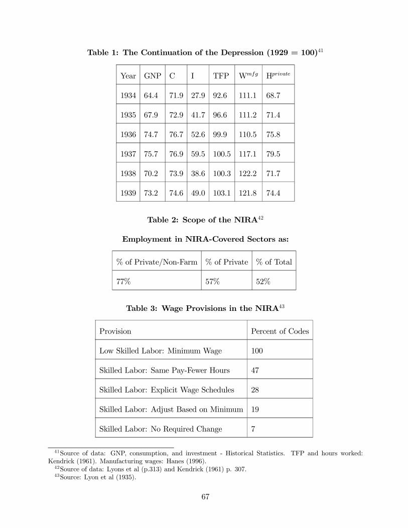
Table 1: The Continuation of the Depression (1929 = 100)41

Year GNP C I TFP Wmfg Hprivate

1934 64.4 71.9 27.9 92.6 111.1 68.7

1935 67.9 72.9 41.7 96.6 111.2 71.4

1936 74.7 76.7 52.6 99.9 110.5 75.8

1937 75.7 76.9 59.5 100.5 117.1 79.5

1938 70.2 73.9 38.6 100.3 122.2 71.7

1939 73.2 74.6 49.0 103.1 121.8 74.4

Table 2: Scope of the NIRA42

Employment in NIRA-Covered Sectors as:

% of Private/Non-Farm % of Private % of Total

77% 57% 52%

Table 3: Wage Provisions in the NIRA43

Provision Percent of Codes

Low Skilled Labor: Minimum Wage 100

Skilled Labor: Same Pay-Fewer Hours 47

Skilled Labor: Explicit Wage Schedules 28

Skilled Labor: Adjust Based on Minimum 19

Skilled Labor: No Required Change 7

41Source of data: GNP, consumption, and investment - Historical Statistics. TFP and hours worked:Kendrick (1961). Manufacturing wages: Hanes (1996).42Source of data: Lyons et al (p.313) and Kendrick (1961) p. 307.43Source: Lyon et al (1935).

67

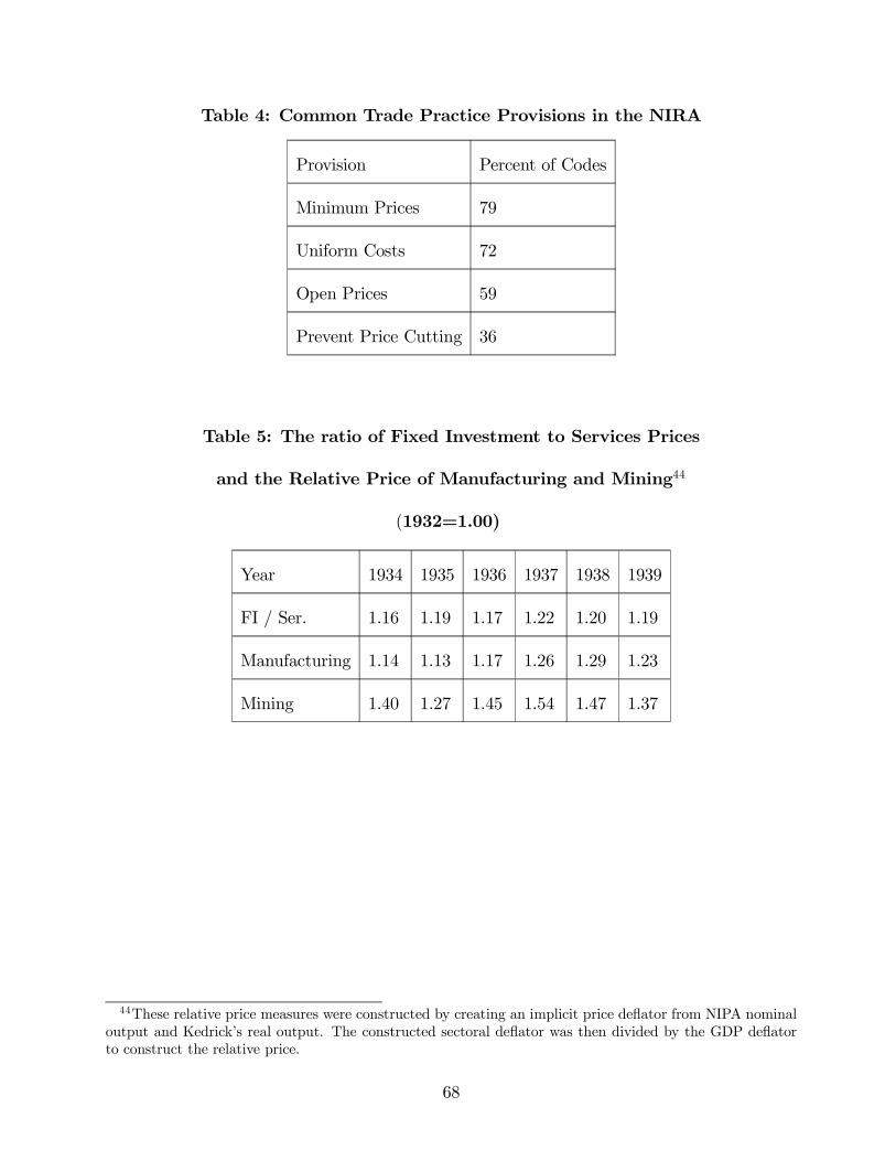
Table 4: Common Trade Practice Provisions in the NIRA

Provision Percent of Codes

Minimum Prices 79

Uniform Costs 72

Open Prices 59

Prevent Price Cutting 36

Table 5: The ratio of Fixed Investment to Services Prices

and the Relative Price of Manufacturing and Mining44

(1932=1.00)

Year 1934 1935 1936 1937 1938 1939

FI / Ser. 1.16 1.19 1.17 1.22 1.20 1.19

Manufacturing 1.14 1.13 1.17 1.26 1.29 1.23

Mining 1.40 1.27 1.45 1.54 1.47 1.37

44These relative price measures were constructed by creating an implicit price deflator from NIPA nominaloutput and Kedrick’s real output. The constructed sectoral deflator was then divided by the GDP deflatorto construct the relative price.

68

Table 6: Disaggregate Price Changes: March 1933 - June 193445

Industry Percent Increase

Petroleum 53

Nonferrous Metals 43

Textiles 42

Leather 28

Building Materials 28

Clothing 26

Home Furnishings 23

Capital Equipment 19

Iron/Steel 16

45Source: Lyon et al and Handbook of Labor Statistics, 1936, Bulletin 616

69

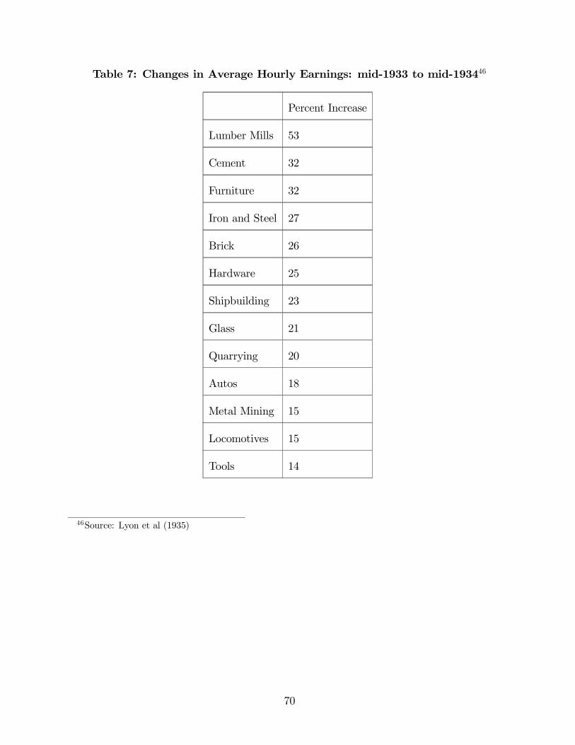
Table 7: Changes in Average Hourly Earnings: mid-1933 to mid-193446

Percent Increase

Lumber Mills 53

Cement 32

Furniture 32

Iron and Steel 27

Brick 26

Hardware 25

Shipbuilding 23

Glass 21

Quarrying 20

Autos 18

Metal Mining 15

Locomotives 15

Tools 14

46Source: Lyon et al (1935)

70

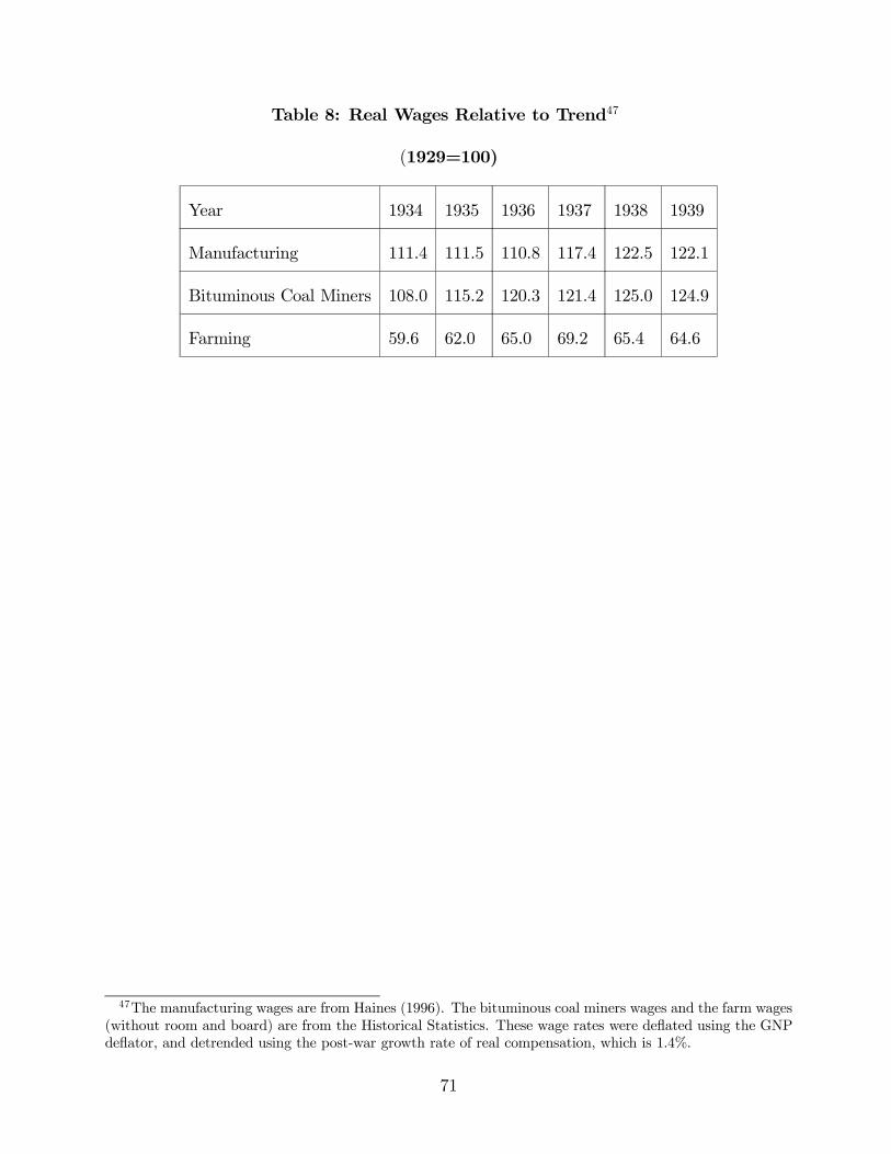
Table 8: Real Wages Relative to Trend47

(1929=100)

Year 1934 1935 1936 1937 1938 1939

Manufacturing 111.4 111.5 110.8 117.4 122.5 122.1

Bituminous Coal Miners 108.0 115.2 120.3 121.4 125.0 124.9

Farming 59.6 62.0 65.0 69.2 65.4 64.6

47The manufacturing wages are from Haines (1996). The bituminous coal miners wages and the farm wages(without room and board) are from the Historical Statistics. These wage rates were deflated using the GNPdeflator, and detrended using the post-war growth rate of real compensation, which is 1.4%.

71

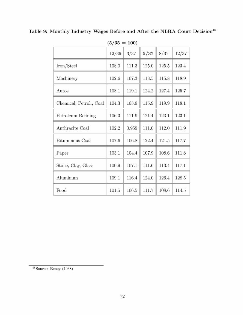
Table 9: Monthly Industry Wages Before and After the NLRA Court Decision48

(5/35 = 100)

12/36 3/37 5/37 8/37 12/37

Iron/Steel 108.0 111.3 125.0 125.5 123.4

Machinery 102.6 107.3 113.5 115.8 118.9

Autos 108.1 119.1 124.2 127.4 125.7

Chemical, Petrol., Coal 104.3 105.9 115.9 119.9 118.1

Petroleum Refining 106.3 111.9 121.4 123.1 123.1

Anthracite Coal 102.2 0.959 111.0 112.0 111.9

Bituminous Coal 107.6 106.8 122.4 121.5 117.7

Paper 103.1 104.4 107.9 108.6 111.8

Stone, Clay, Glass 100.9 107.1 111.6 113.4 117.1

Aluminum 109.1 116.4 124.0 126.4 128.5

Food 101.5 106.5 111.7 108.6 114.5

48Source: Beney (1938)

72

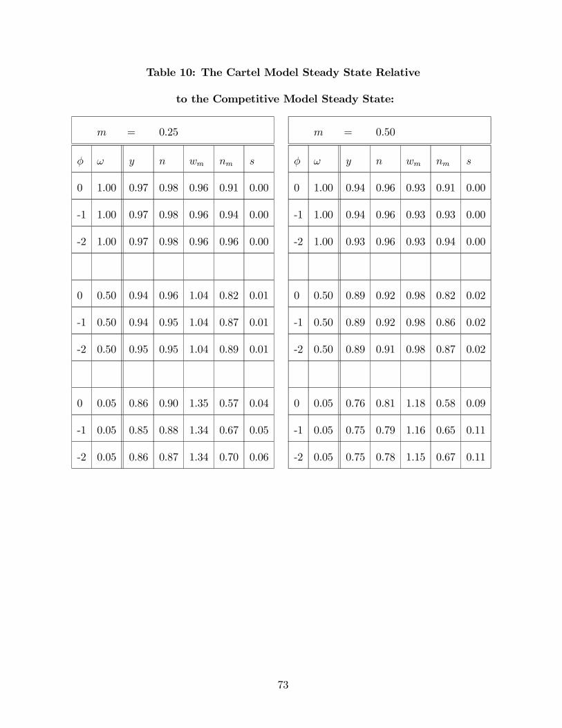
Table 10: The Cartel Model Steady State Relative

to the Competitive Model Steady State:

m = 0.25

φ ω y n wm nm s

0 1.00 0.97 0.98 0.96 0.91 0.00

-1 1.00 0.97 0.98 0.96 0.94 0.00

-2 1.00 0.97 0.98 0.96 0.96 0.00

0 0.50 0.94 0.96 1.04 0.82 0.01

-1 0.50 0.94 0.95 1.04 0.87 0.01

-2 0.50 0.95 0.95 1.04 0.89 0.01

0 0.05 0.86 0.90 1.35 0.57 0.04

-1 0.05 0.85 0.88 1.34 0.67 0.05

-2 0.05 0.86 0.87 1.34 0.70 0.06

m = 0.50

φ ω y n wm nm s

0 1.00 0.94 0.96 0.93 0.91 0.00

-1 1.00 0.94 0.96 0.93 0.93 0.00

-2 1.00 0.93 0.96 0.93 0.94 0.00

0 0.50 0.89 0.92 0.98 0.82 0.02

-1 0.50 0.89 0.92 0.98 0.86 0.02

-2 0.50 0.89 0.91 0.98 0.87 0.02

0 0.05 0.76 0.81 1.18 0.58 0.09

-1 0.05 0.75 0.79 1.16 0.65 0.11

-2 0.05 0.75 0.78 1.15 0.67 0.11

73

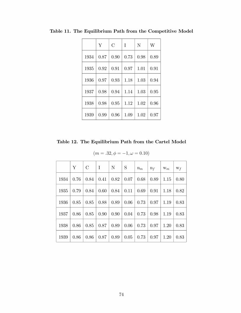
Table 11. The Equilibrium Path from the Competitive Model

Y C I N W

1934 0.87 0.90 0.73 0.98 0.89

1935 0.92 0.91 0.97 1.01 0.91

1936 0.97 0.93 1.18 1.03 0.94

1937 0.98 0.94 1.14 1.03 0.95

1938 0.98 0.95 1.12 1.02 0.96

1939 0.99 0.96 1.09 1.02 0.97

Table 12. The Equilibrium Path from the Cartel Model

(m = .32,φ = −1,ω = 0.10)

Y C I N S nm nf wm wf

1934 0.76 0.84 0.41 0.82 0.07 0.68 0.89 1.15 0.80

1935 0.79 0.84 0.60 0.84 0.11 0.69 0.91 1.18 0.82

1936 0.85 0.85 0.88 0.89 0.06 0.73 0.97 1.19 0.83

1937 0.86 0.85 0.90 0.90 0.04 0.73 0.98 1.19 0.83

1938 0.86 0.85 0.87 0.89 0.06 0.73 0.97 1.20 0.83

1939 0.86 0.86 0.87 0.89 0.05 0.73 0.97 1.20 0.83

74

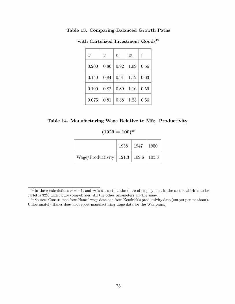
Table 13. Comparing Balanced Growth Paths

with Cartelized Investment Goods49

ω y n wm i

0.200 0.86 0.92 1.09 0.66

0.150 0.84 0.91 1.12 0.63

0.100 0.82 0.89 1.16 0.59

0.075 0.81 0.88 1.23 0.56

Table 14. Manufacturing Wage Relative to Mfg. Productivity

(1929 = 100)50

1938 1947 1950

Wage/Productivity 121.3 109.6 103.8

49In these calculations φ = −1, and m is set so that the share of employment in the sector which is to becartel is 32% under pure competition. All the other parameters are the same.50Source: Constructed from Hanes’ wage data and fromKendrick’s productivity data (output per manhour).

Unfortunately Hanes does not report manufacturing wage data for the War years.)

75