New Deal Policies and Recovery from the Great Depression

by

Joshua Kautsky Hausman

A dissertation submitted in partial satisfaction of the

requirements for the degree of

Doctor of Philosophy

in

Economics

in the

Graduate Division

of the

University of California, Berkeley

Committee in charge:

Professor Barry Eichengreen, Co-ChairProfessor J. Bradford DeLong, Co-Chair

Professor Christina RomerProfessor Maurice ObstfeldProfessor Noam Yuchtman

Spring 2013

New Deal Policies and Recovery from the Great Depression

Copyright 2013by

Joshua Kautsky Hausman

1

Abstract

New Deal Policies and Recovery from the Great Depression

by

Joshua Kautsky Hausman

Doctor of Philosophy in Economics

University of California, Berkeley

Professor Barry Eichengreen, Co-Chair

Professor J. Bradford DeLong, Co-Chair

What forces led to rapid recovery of the U.S. economy after 1933? Why was recoveryderailed by a severe recession in 1937? Since Friedman and Schwartz (1963), economists haveemphasized monetary explanations. This dissertation shows that in three crucial instancesother factors mattered. Methodologically, it demonstrates the value of using micro data toexplore macro questions.

The first chapter considers the effect of the 1936 veterans’ bonus. Conventional wisdomhas it that in the 1930s fiscal policy did not work because it was not tried. This chapter showsthat fiscal policy, though inadvertent, was tried in 1936, and a variety of evidence suggeststhat it worked. A deficit-financed veterans’ bonus provided 3.2 million World War I veteranswith cash and bond payments totaling 2 percent of GDP; the typical veteran received apayment equal to annual per capita personal income. This chapter uses time-series andcross-sectional data to identify the effects of the bonus. I exploit four sources of quantitativeevidence: a detailed household consumption survey, cross-state and cross-city regressions,aggregate time-series, and a previously unused American Legion survey of veterans. Theevidence paints a consistent picture in which veterans quickly spent the majority of theirbonus. Spending was concentrated on cars and housing in particular. Narrative accountssupport these quantitative results. A back-of-the-envelope calculation suggests that thebonus added 2.5 to 3 percentage points to 1936 GDP growth.

In my second chapter, I consider the causes of the severe recession that followed theboom year of 1936. The 1937-38 recession was one of the largest in U.S. history. Industrialproduction fell 32 percent and the nonfarm unemployment rate rose 6.6 percentage points.This paper shows that there were timing, geographic, and sectoral anomalies in the recession,none of which are easily explained by aggregate macro shocks. I argue that a supply shockin the auto industry contributed both to the recession’s anomalies and to its severity. Labor-strife-induced wage increases and an increase in raw material costs led auto manufacturersto raise prices in the fall of 1937. Equally important, higher costs combined with nominalrigidity to make the price increase predictable. Expectations of price increases brought auto

2

sales forward and thus sustained sales during the summer and early fall of 1937, despitenegative monetary and fiscal factors. When auto prices did rise in October and November,sales and production plummeted. A forecasting exercise suggests that in 1938, this shockreduced auto sales by 600,000 and GDP growth by 1.2 percentage points.

In my third chapter, I consider the miraculous recovery of the U.S. economy duringFranklin Roosevelt’s first months in office. From March to July 1933, industrial productionrose 57 percent, by far the most rapid increase since records began. The recovery wasconcentrated in durable goods industries, particularly autos. Using a novel dataset, I showthat auto sales increased much more rapidly in farm than in nonfarm states in spring 1933.This suggests that dollar devaluation may have directly spurred recovery by raising farmincomes. The negative effect of higher crop prices on urban consumers may have been offsetby the positive effect of higher crop prices on expected inflation.

i

To Catie and Alex.

ii

Contents

Introduction 1

1 The Veterans’ Bonus of 1936 61.1 Introduction . . . . . . . . . . . . . . . . . . . . . . . . . . . . . . . . . . . . 61.2 Background on the veterans’ bonus . . . . . . . . . . . . . . . . . . . . . . . 101.3 Evidence from the 1935-36 Study of Consumer Purchases . . . . . . . . . . 141.4 Cross-state and cross-city evidence . . . . . . . . . . . . . . . . . . . . . . . 291.5 Direct survey and narrative evidence . . . . . . . . . . . . . . . . . . . . . . 401.6 Why was the MPC so high? . . . . . . . . . . . . . . . . . . . . . . . . . . . 461.7 Aggregate effects of the bonus . . . . . . . . . . . . . . . . . . . . . . . . . . 491.8 Conclusion . . . . . . . . . . . . . . . . . . . . . . . . . . . . . . . . . . . . 53A Appendix . . . . . . . . . . . . . . . . . . . . . . . . . . . . . . . . . . . . . 54

2 The Auto Industry and the 1937-38 Recession 672.1 Introduction . . . . . . . . . . . . . . . . . . . . . . . . . . . . . . . . . . . . 672.2 Previous literature and policy developments . . . . . . . . . . . . . . . . . . 702.3 Anomalies . . . . . . . . . . . . . . . . . . . . . . . . . . . . . . . . . . . . . 732.4 An auto industry supply shock . . . . . . . . . . . . . . . . . . . . . . . . . . 852.5 How did the price shock impact sales? . . . . . . . . . . . . . . . . . . . . . 922.6 Can the auto price shock explain the recession’s anomalies? . . . . . . . . . . 992.7 Conclusion . . . . . . . . . . . . . . . . . . . . . . . . . . . . . . . . . . . . . 105A Appendix . . . . . . . . . . . . . . . . . . . . . . . . . . . . . . . . . . . . . 107

3 Growth After a Financial Crisis: The U.S. in Spring 1933 1083.1 Introduction . . . . . . . . . . . . . . . . . . . . . . . . . . . . . . . . . . . . 1083.2 Aggregate data . . . . . . . . . . . . . . . . . . . . . . . . . . . . . . . . . . 1113.3 Geographical variation of auto sales . . . . . . . . . . . . . . . . . . . . . . . 1193.4 Implications . . . . . . . . . . . . . . . . . . . . . . . . . . . . . . . . . . . 1243.5 Conclusion . . . . . . . . . . . . . . . . . . . . . . . . . . . . . . . . . . . . . 131

Conclusion 132

References 135

iii

Acknowledgments

I cannot imagine a better dissertation committee for a macrohistorian. Barry Eichengreenmet with me nearly every week for the past three years. He patiently guided me through theprocess of focusing my interests and landing on a first topic. By my count, he read at leastten drafts of my work. Each time, he provided detailed comments on major and minor points.It is no exaggeration to say that Barry taught me both how to write a paper and how to doeconomic history. I learned from Barry how an economic historian can combine an attentionto context and data quality with relevance to economics and policy more broadly. Equallyimportant, Barry gave me a model of how to juggle the many obligations of academic life,how to prioritize research while at the same time fulfilling other obligations conscientiously.How someone so productive can be so helpful and available remains a mystery to me.

I am equality indebted to Christina Romer. In the fall of my second year, I took hercourse (co-taught with David Romer) on “Macroeconomic History.” I learned that greateconomic history can also be great macroeconomics, that I did not need to choose betweenmy interests in history and macro. Near the end of the course, Christina was picked to be thenext chair of the Council of Economic Advisers. I cannot imagine a better demonstration ofthe relevance of economic history for contemporary policy.

In 2009-10 I worked as a staff economist at the CEA. There, with much help fromChristina, I learned how to understand macro data and the importance of careful fact-checking in empirical work. Soon after I returned to Berkeley in summer 2010, so didChristina. Since then, her advice has been invaluable. She encouraged me to go after bigquestions and trust that I would find a way to answer them. And her careful reading of mywork helped me express my thoughts far more clearly. Finally, Christina’s enthusiasm andencouragement sustained my morale at times when research problems felt insurmountable.

Brad DeLong taught me economic history my first year. I still remember his erudite andgripping lectures. They convinced me to be an economic historian. In my second year, heindulged my excitement about economic history by conducting a reading course with meas the only student! Since then, he has been a constant source of wisdom. His instinctsabout what topics would be fruitful were uncanny. He pushed me to continue work on theveterans’ bonus even when the path forward was unclear. And Brad’s knowledge aboutalmost everything improved each chapter of this dissertation.

Maury Obstfeld taught me the macroeconomics of consumption in my first year andinternational finance in my second. He gave me a model of how to do technically sophisticatedmacroeconomics grounded in an understanding of the real world. Maury also chaired myorals examination committee and provided weekly advice as I frantically prepared for oralsin advance of going to work at the CEA. While working on my dissertation, Maury wasalways available to discuss matters large and small. His advice on how my empirical findingsmight be reconciled with macro theory was often invaluable.

Noam Yuchtman was a late but essential addition to my committee. As the only appliedmicroeconomist, he gave me much needed advice on how to improve my empirical work.But his help went beyond this. He carefully read drafts and gave me feedback on items

iv

ranging from typos to motivation. Despite being himself a new assistant professor, Noamwas remarkably generous with his time, often sitting with me for an hour to discuss anempirical problem or advise me on what I should prioritize. My dissertation is far strongerfor this.

Four professors not on my committee deserve special recognition. David Romer joinedmany of my conversations with Christina. He often showed me how to solve a problem in asimple, straightforward way. More than anyone, David helped me to see how to relate mywork on the veterans’ bonus to the broader literature on fiscal multipliers.

Yuriy Gorodnichenko was exceptionally generous to me with his time and advice. Heboth advised me on what questions would be of general interest to macroeconomists andwas a source of answers on all technical questions. Finally, Yuriy’s macro lunch provided mewith opportunities to present my work.

Like the macro lunch, Marty Olney’s history lunch gave me a chance to present earlystages of my work. And Marty was a perpetual source of advice on all matters economic-history related. Her expertise on interwar-era consumption, and household consumptionsurveys in particular, was much appreciated.

George Akerlof taught me macro my first year then hired me as a research assistantto help him with his books Animal Spirits and Identity Economics. This was a formativeexperience that taught me an enormous amount of economics.

Many other Berkeley faculty members helped me with specific questions and inspired mewith their courses. Among others, I would like to thank George Akerlof, Max Auffhammer,Severin Borenstein, David Card, Jan De Vries, Shachar Kariv, Demian Pouzo, James Powell,Michael Reich, and Richard Sutch.

I owe my classmates more than I can easily describe. Gabriel Chodorow-Reich has beena friend since first year, a colleague at the CEA, and a constant source of wisdom on matterslarge and small. He gets credit for the title of my second chapter. Over Asian food andcoffee, Johannes Wieland, John Mondragon and Dominick Bartelme became good friendsand taught me much of what I know about macro. I lived next door to Alexandre Poiriermy first year, and since then he has patiently helped me to understand the mysteries ofeconometrics. Among others, Mark Borgschulte, Issi Romem, and Owen Zidar also provideduseful comments on parts of this work. Jeremiah Dittmar, Shari Eli, Andy Jalil, LorenzKueng, Jonathan Rose, and Mu-Jeung Yang departed Berkeley before me and gave me anexample to follow. Nicolas Ziebarth likewise provided an example of how to be a successfulyoung macrohistorian.

Last but far from least, I thank my family. My wife Catie was a constant help. Asa superb empirical economist, her penetrating questions and detailed advice pushed me toimprove my work and make it more accessible to economists outside of economic historyor macroeconomics. Her calm and wisdom preserved my sanity during the more difficultmoments of graduate school.

My father, Daniel Hausman, and brother, David Hausman, read drafts of chapters andprovided a useful perspective on my work from outside economics. My mother, Cathy

v

Kautsky, reminded me that there is more to life than economics, and provided essentialencouragement to me throughout graduate school.

In addition to the help I received at Berkeley, Chapter 1 benefited from the commentsof seminar participants at the All-UC Graduate Student Workshop, the fall 2012 MidwestMacro Meetings, the University of Iowa, the Office of Financial Research at the TreasuryDepartment, Dartmouth College, Wellesley College, Johns Hopkins University, the Univer-sity of Calgary, the University of Michigan, the Federal Reserve Board, and the University ofColorado, Boulder. For this chapter, I also thank the American Legion library for providingme with unpublished tabulations of their 1936 survey and Price Fishback for providing mewith a digital copy of the BLS residential building permit data.

Chapter 2 benefited from comments of seminar participants at the All-UC Group Con-ference on Transport, Institutions, and Economic Performance at UC Irvine.

1

Introduction

The U.S. recovery from the Great Depression was nearly as exceptional as the Depressionitself. When Franklin Roosevelt took office in March 1933, the unemployment rate was 21percent, real GNP per capita was lower than it had been in 1907, and much of the bankingsystem had collapsed.1 The Depression had done much to discredit American democracy.The prominent columnist Walter Lippmann argued, not atypically, that “A mild species ofdictatorship will help us over the roughest spots in the road ahead” (qtd. in Alter 2007,p. 187). Yet seven years later, in 1940, American democratic institutions were intact. Theunemployment rate had fallen to 9.5 percent and GNP per capita had grown 54 percent.Productivity had advanced at an unprecedented pace (Field 2011). But recovery had notbeen uniform. It was interrupted by a severe recession in 1937-38 in which the unemploymentrate rose more than 3 percentage points.

Economic historians have long been interested in what caused the 1929 to 1933 U.S.downturn, but comparatively little work examines the recovery that followed.2 This disser-tation helps fill this gap. It adds to our understanding both of the rapid recovery and ofthe double-dip recession. I consider three episodes that illuminate the role of fiscal policy,unionization, and devaluation in this period. The first chapter examines the effects of a 2percent of GDP fiscal stimulus program, the veterans’ bonus of 1936. I document that fiscalpolicy worked: veterans spent a large share of their bonus. The second chapter examinesthe causes of the severe recession that followed the boom year of 1936. I show that a sup-ply shock in the auto industry helps to explain the recessions’ severity as well as its timingand geographic incidence. Finally, in the third chapter, I consider the sources of recoveryduring Franklin Roosevelt’s first months in office. Just as a shock to the relative price ofautos played an important role in returning the economy to recession in 1937, I suggest thatchanges to the relative price of farm products may have been crucial to rapid recovery inspring 1933.

In addition to its focus on a common time and place, two themes unify this work. First, allthree papers show the importance of non-monetary factors during the 1930s. GDP growth of13 percent in 1936 and -3 percent in 1938 can only be explained by the interaction of monetary

1The unemployment rate is from Darby (1976). Real GNP data are from Romer (1989) and NIPA ta-ble 1.7.6. Population data are from http://www.census.gov/popest/data/national/totals/pre-1980/

tables/popclockest.txt.2Exceptions include Cole and Ohanian 2004, Eggertsson 2008, and Romer 1992.

2

factors with fiscal policy and exogenous developments in the auto industry. Chapter threesuggests that rapid recovery in spring 1933 was due in part to the relative price effects onfarmers of dollar devaluation. To be clear, none of these chapters disputes the primaryimportance of monetary factors in explaining recovery and the double-dip recession. Rather,I show that at crucial times, non-monetary factors mattered.

The second theme of this dissertation is the role of the auto industry as an amplifyingmechanism for demand and supply shocks. The veterans’ bonus had large effects becauseveterans used their money to buy cars. Unionization in 1937 interacted with price-settingpractices in the auto industry to create a large macro shock. And in spring 1933, autoproduction grew far more rapidly than industrial production as a whole, in part spurred byfarmers enjoying higher crop prices.

Typically, such industry-specific factors are absent from economists’ accounts of this pe-riod. The existing literature emphasizes either the economy’s automatic recovery mechanismsor the importance of monetary policy. Some authors argue that output growth after 1933reflected the disappearance of temporary negative shocks (DeLong and Summers 1988) orthe economy’s strong self-correcting mechanisms (Bernanke and Parkinson 1989, Friedmanand Schwartz 1963). Other authors dispute that there was anything natural or inevitableabout rapid recovery post-1933. Eichengreen and Sachs (1985) do not focus on the U.S.experience, but their finding that across countries devaluation was positively correlated withrecovery suggests that monetary factors were important. Romer (1992) forcefully articulatesthe case for a monetary explanation of U.S. recovery. She finds that “rapid rates of growthof real output in the mid- and late 1930s were largely due to conventional aggregate-demandstimulus, primarily in the form of monetary expansion” (p. 757). Romer complements earlierwork by Temin and Wigmore (1990) who argue that the departure of the U.S. from the GoldStandard in April 1933 was a monetary regime change. Eggertsson (2008) formalizes thisargument. In the context of a DSGE model, Eggertsson shows how Roosevelt’s actions, byraising expected inflation and thus lowering the real interest rate, could have spurred rapidgrowth.

Just as expansionary monetary policy is often thought to explain rapid growth from1933 to 1937, contractionary monetary policy is the most popular explanation for the 1937-38 recession.3 The Federal Reserve raised reserve requirements in August 1936 and againin March and May 1937. In December 1936, the Treasury began sterilizing gold inflows.Friedman and Schwartz argue (1963, pp. 544-545):

The combined impact of the rise in reserve requirements and–no less important–the Treasury gold-sterilization program first sharply reduced the rate of increasein the money stock and then converted it into a decline. . . . The sharp retar-dation in the rate of growth of the money stock must surely have been a factorcurbing expansion, and the absolute decline, a factor intensifying contraction.

3See, for example, Roose (1954), Friedman and Schwartz (1963), Eichengreen (1992), Romer (1992),Velde (2009), and Irwin (2011). Some authors have also considered contractionary fiscal policy as a possiblecause of this recession. See chapter 2.

3

There is an emerging consensus that the key shock was the Treasury gold sterilizationrather than the increase in reserve requirements. Irwin (2011) estimates that absent goldsterilization, in 1937 the monetary base would have been as much as 10 percent larger. Thechannel through which money supply declines impacted real activity in 1937-38 is, however,unclear. There was relatively little effect on interest rates. Yields briefly spiked by 10 to 40basis points in the spring and summer of 1937, but remained close to zero over the period.

Of course when interest rates are near zero, monetary policy can still change expectationsof inflation, and thus affect the real interest rate and the real economy. This is the chan-nel through which Eggertsson (2008) and Romer (1992) argue that policy led to economicrecovery after 1933. Eggertsson and Pugsley (2006) argue that policymakers’ actions in thespring of 1937 lowered inflation expectations, and through this channel, caused the 1937-1938recession. This provides one way of explaining how monetary actions, despite little impacton interest rates, may have had large contractionary effects.

This brief tour of the literature suggests a unified monetarist interpretation of the 1930s:when money growth was rapid, as it was from 1933 through 1936, and again after 1938,growth was rapid. When money growth slowed, as it did in 1937-38, so did growth. We shallsee that this story is too simple.

The first chapter considers fiscal policy. The conventional wisdom has it that in the 1930sfiscal policy did not work because it was not tried. In this paper, I show that fiscal policy,though inadvertent, was tried in 1936, and a variety of evidence suggests it worked. In June1936, a deficit-financed veterans bonus provided 3.2 million World War I veterans with cashand bond payments totaling 2 percent of GDP; the typical veteran received a payment equalto annual per capita personal income, enough money to buy a new car.

This paper uses cross-sectional data to identify the effects of the bonus. I exploit foursources of quantitative evidence: a detailed household consumption survey, cross-state andcross-city regressions, aggregate time-series, and a previously unused American Legion surveyof veterans. The evidence paints a consistent picture in which veterans quickly spent themajority of their bonus. The point estimate of the marginal propensity to consume is 0.7,with at least half this spending on cars and housing. Combined with a reasonable estimateof the multiplier, this suggests that the bonus added 2.5 to 3 percentage points to 1936 GDPgrowth.

This chapter contributes both to the economic history of the 1930s, and to the litera-ture on the consumption effects of fiscal transfers. In particular, I show that the marginalpropensity to consume can be high even when transfer payments are very large. I argue thatfeatures of the 1936 economy, some unique to the time, some generally present in economicrecoveries, were conducive to large effects from a transfer payment. Liquidity constraintswere pervasive and were made binding by expectations of higher future income. Stocks ofautos and housing were low, so many households chose to buy a car or house rather thansave their bonus. Indeed, receiving the bonus made veterans 22 percentage points more likelyto purchase a car. Finally, since interest rates were at the zero lower bound, the spendingmultiplier is likely to have been high.

Thus the effect of the bonus was not independent of the state of the economy. In particu-

4

lar, it mattered that the share of the population that owned cars was large and growing.4 Inchapter two, I argue that the auto industry was sufficiently large to play a central role in the1937-38 recession. The conventional wisdom blames the double-dip recession on monetarycontraction, and to a lesser extent on the backside of the veterans’ bonus and the instatementof social security taxes. But while these factors were undoubtedly important, in the firsthalf of this chapter I show that there are in fact timing, geographic, and sectoral anomaliesin the recession not easily explained by macro policy. Specifically:

• The decline in industrial production from September to December 1937 is the largestthree-month decline in the history of the Federal Reserve and Miron-Romer series goingback to 1884.

• Manufacturing employment rises in 8 states despite a 12 percent decline nationwide.

• There is a lack of comovement between components of GDP. Durables consumptionfalls over 17 percent while nondurables consumption rises. The 1937-38 recession isthe only time since the Great Depression in which nondurables spending rises in arecession in which annual real GDP falls more than 2 percent.

My analysis points strongly to a role for the auto industry in explaining the unusualfeatures of the recession: manufacturing employment falls most in Michigan, and auto pro-duction falls by nearly 50 percent. Furthermore, auto prices rise while the economy-wideprice level falls. In the second half of the chapter, I ask what explains the peculiar behaviorof the auto industry, and how exogenous developments in this industry affected the rest ofthe economy. I argue that a cost shock and consequent auto price increases explain thecollapse of car sales and production. Unionization and an increase in raw material costsled auto manufacturers to raise prices in fall 1937. Equally important, the increase in costscombined with nominal rigidity to make the price increase predictable. Expectations of priceincreases brought auto sales forward and thus sustained sales during the summer and earlyfall of 1937, despite negative monetary and fiscal factors. When auto prices did increase infall 1937, sales plummeted. Narrative evidence confirms this story.

To quantify the effect on auto sales, I perform a forecasting exercise. Using criteria thatpenalize overfitting, I choose the model that best matches the monthly pre-recession behaviorof auto sales given fiscal and monetary factors and overall economic conditions. As expected,the model underpredicts sales in the summer of 1937, when consumers expected auto pricesto soon increase, and overpredicts sales in 1938. This exercise implies that without theexpected increase in auto prices, the fall in auto sales between 1937 and 1938 would havebeen 0.8 million rather than the actual 1.6 million. Using data on the price of cars soldand an estimate of the multiplier, I find that positive price expectations added 0.3 percent

4In 1935, there was roughly one car on the road for every 6 people in the country; the population was127 million and there were 22.5 million cars registered. Population data are from http://www.census.

gov/popest/data/national/totals/pre-1980/tables/popclockest.txt; car registration data are fromNBER macrohistory series a01108.

5

to GDP in 1937, while the subsequent drop-off in sales subtracted 1.0 percent from GDPin 1938: absent the shock, the output decline in 1938 would have been more than a thirdsmaller.

This paper contributes to our understanding of the severe 1937-38 recession and providesan unusually clear example of how supply shocks can affect the economy. It also showsthat even before World War II, the auto industry was sufficiently large for fluctuations inproduction and sales to have important aggregate effects.5

Perhaps surprisingly, the 1937-38 recession may also help us understand the 1933 recov-ery. My third chapter considers the causes of U.S. growth in the immediate aftermath ofRoosevelt’s inauguration. From its low point in March 1933, seasonally adjusted industrialproduction rose 57 percent in four months.6 The existing literature has emphasized two ex-planations for the economy’s emergence from the Depression in spring 1933: first, the effectsof Franklin Roosevelt’s words and actions on inflation expectations, and second, the directeffects of the dollar’s devaluation on farmers. Both explanations can in theory explain theeconomy’s turn-around and the concentration of the recovery in durable goods’ industries,particularly autos.

It has been difficult to know whether there was a distinct channel leading to recoverythrough agriculture absent high frequency geographically disaggregated data. We have notknown whether recovery proceeded more or less rapidly in North Dakota or in New York. Thecontribution of this chapter is to provide such data and to use it to test whether recoveryproceeded more quickly in agricultural states. I exploit a previously unused dataset ofmonthly, state level auto sales to examine whether the share of a state population’s engagedin farming was correlated with auto sales recovery in spring 1933. I find that it was. Aone standard deviation increase in the share of a state’s population living on farms wasassociated with roughly a 25 percentage point increase in auto sales growth from late winterto early summer 1933. In aggregate, my results imply that the recovery, at least as measuredby auto sales, might have been as much as 50 percent slower if farm demand had not grownmore rapidly than demand in the economy as a whole.

As in 1937, price expectations may have been an important transmission channel. Ihypothesize that although higher crop prices only directly benefited the 25 percent of thepopulation in agriculture,7 they may have contributed to consumer expectations of futureprice increases. This in turn could have boosted consumer demand in urban and rural areas.An attraction of this explanation is that it can explain both the consumption and productionboom in spring 1933 and the subsequent partial reversal in late summer 1933. Expectationsof price increases would have meant more goods sold in spring 1933 and fewer sold in summerand fall.

5Ramey and Vine (2006) document the importance of the auto industry to postwar fluctuations.6FRED series INDPRO.7Share of the population in agriculture is taken from the 5% IPUMS sample of the 1930 Census.

6

Chapter 1

Fiscal Policy and Economic Recovery:The Case of the 1936 Veterans’ Bonus

“The gov’t last week paid a soldiers’ bonus of over two billion and as a resultthe veterans have been buying cars, clothing, etc. Streets are crowded and thehighways are jammed with new cars. It begins to look like old times again.”- Benjamin Roth’s diary, 6/25/1936 (Roth 2009, p. 172).

1.1 Introduction

After falling 27 percent between 1929 and 1933, real GDP rose by 43 percent between 1933and 1937. Indeed, the economy grew more rapidly between 1933 and 1937 than it hasduring any other four year peacetime period since at least 1869.1 The most rapid growthcame in 1936, when real GDP grew 13.1 percent and the unemployment rate fell 4.4 per-centage points.2 Conventional explanations of the rapid recovery emphasize the economy’sself-correcting mechanisms and the effect of expansionary monetary policy and resultingexpectations of inflation. The literature almost universally dismisses fiscal policy as a pri-mary source of recovery before World War II.3 Economists have generally accepted E. CaryBrown’s (1956) statement that “Fiscal policy . . . seems to have been an unsuccessfulrecovery device in the ’thirties–not because it did not work, but because it was not tried”(pp. 863-866).

In fact, this chapter demonstrates that fiscal policy, though inadvertent, was tried in1936, and a variety of evidence suggests that it worked. The government paid a large bonusto World War I veterans in June 1936, and within six months veterans spent roughly 70

1Data are from NIPA table 1.1.6 and Romer (1989).2NIPA table 1.1.1 and Darby 1976.3Eggertsson (2008) argues that deficit spending under Roosevelt helped make monetary expansion cred-

ible and thus contributed to higher inflation expectations. But like other authors, Eggertsson does notemphasize the direct stimulative effects of fiscal policy in the 1930s.

7

cents out of every dollar received. A back-of-the-envelope calculation suggests that absentthe veterans’ bonus, GDP growth in 1936 would have been about 2.5 to 3 percentage pointsslower and the unemployment rate 1.3 to 1.5 percentage points higher.

After years of demonstrations and lobbying by veterans’ groups, in 1936 congress au-thorized a deficit-financed payment of $1.8 billion to 3.2 million World War I veterans.4

The bonus was 2.1 percent of 1936 GDP,5 roughly the same magnitude as annual spendingfrom the American Recovery and Reinvestment Act (the Obama stimulus) in 2009 and 2010(Council of Economic Advisers 2010). The typical veteran received $550 dollars, more thanannual per capita income,6 and enough money to buy a new car.7 Given its size, economichistorians have sometimes suspected that the bonus had a positive impact on 1936 growth.However, there is almost no systematic work analyzing the effects of the bonus. Only onepaper, Telser (2003), examines the veterans’ bonus in detail. Telser studies a variety of timeseries and concludes that the bonus “brought a large measure of recovery to the economy”(p. 240).8 But although a useful start, Telser’s work is limited by his exclusive use of timeseries evidence. Since the bonus was a one-time event, this makes it impossible for Telser toconduct formal statistical tests of the bonus’s impacts.

In addition to revisiting the time series data, I exploit three other sources of evidence onthe bonus’s effects. First, I use a 1935-36 household consumption survey to estimate veterans’marginal propensity to consume (MPC) out of the bonus. Since this consumption surveydid not ask about respondents’ veteran status, I use a two-step estimator with auxiliaryinformation from the 1930 census. The consumption survey has information on the age,race, and location of each household. These variables also appear in the 1930 census, alongwith an indicator for World War I veteran status. In the first step I estimate the relationshipbetween veteran status and age, race, and location. The second step relates these predictedvalues - the probability a household contains a veteran - to the change in consumption preto post bonus payment. I outline a proof that, given a set of reasonable assumptions, thisprocedure provides consistent estimates of spending from the bonus.

The robust result is that the MPC was between 0.6 and 0.75. This high MPC likely re-flects the state of the economy in 1936, in particular the combination of liquidity constraints,expectations of higher future income, and a low stock of durables. The household consump-tion survey also allows me to estimate marginal propensities to consume for subcategories ofconsumption. These estimates imply that veterans spent almost a quarter of their bonus oncar purchases and vehicle operations. The bonus increased the probability of a car purchase

4Data on bonus amount and number of veterans are from Veterans’ Administration 1936, pp. 23-24.5This is the ratio of the bonus to 1936 nominal GDP (NIPA table 1.1.5).6Per capita personal income was $535 in 1936 (NIPA table 2.1).7According to Automotive Industries, 11/14/36, p. 666 the price of the cheapest Ford and cheapest

Chevrolet in 1936 was $510.8Using annual regressions, Telser finds evidence that federal deficits were correlated with consumption

growth in the 1930s, evidence he interprets as supportive of a large effect of the bonus. Telser also graphicallyexamines monthly data on industrial production, wholesale prices, and department store sales. He arguesthat department store sales in particular suggest large effects of the bonus.

8

by 22 percentage points relative to a baseline probability of purchasing a car of less than20 percent. Results also suggest substantial spending on housing consumption. Estimatesfor other categories of consumption are less precise but point to spending on furniture /appliances, clothing, recreation, and food.

A third source of evidence on the bonus’s effects are cross-state and cross-city regressions.Significant variation in the share of veterans in a state or city’s population meant significantvariation in the fiscal stimulus received in 1936. As expected given the household surveyresults, there is a strong relationship across states between veterans per capita and the changein car sales in 1936. On average, one additional veteran in a state was associated with 0.3more new cars sold. There is also a strong association between the proportion of a city’spopulation made up of veterans and the change in residential building permits from 1935to 1936. An additional veteran in a city was associated with at least $100 more residentialbuilding.

By comparison, cross-state regressions provide little useful information on the bonus’semployment impacts. This is not surprising. Insofar as veterans spent their bonus on durable,traded goods like cars, large aggregate effects would be consistent with no relationship atthe state level. In fact, employment in Michigan grows far more in 1936 than in any otherstate, exactly as one would expect given the boom in new car sales induced by the bonus.9

A final source of evidence on veterans’ spending behavior comes from an unpublishedAmerican Legion survey that asked 42,500 veterans how they planned to use their bonus.Veterans told the American Legion that they planned to consume 40 cents out of everydollar and to spend an additional 25 cents out of every dollar on residential and businessinvestment. Evidence from the 2001 and 2008 tax rebates suggests that such ex ante surveysmay understate spending. Thus the prospective MPC of 0.4 measured in the AmericanLegion Survey suggests that the actual MPC was probably higher. It is evidence that theMPC of 0.6 to 0.75 that I measure in the household consumption survey is not an artifactof the particular sample or estimation method.

Neither household survey nor cross-state estimates of the bonus’s effects translate directlyinto a measure of the bonus’s aggregate impact. The effect of the bonus on the economy asa whole was a function not only of the recipients’ MPC, but of general equilibrium effectsthat could have amplified or diminished the initial spending impulse. A plausible simplecalculation suggests that the multiplier associated with the bonus was slightly above one,and hence that the bonus added 2.5 to 3 percentage points to 1936 GDP growth.

This chapter contributes to two literatures. The first is on what explains rapid U.S.growth after 1933.10 Some authors argue that output growth after 1933 reflected the disap-pearance of temporary negative shocks (DeLong and Summers 1988) or the economy’s strong

9These results can be compared to those in Fishback and Kachanovskaya (2010). They examine thecross-state multiplier from all types of federal spending in the 1930s. Like me, they find large effects on autosales, but their results for income and employment are mixed, possibly reflecting the effects of spillovers.

10Cole and Ohanian (2004) argue that the recovery was in fact weak. This is in part because theyemphasize the position of the economy in 1939 relative to that in 1933, and thus incorporate in theircomparison the ground lost during the 1937-38 recession.

9

self-correcting mechanisms (Bernanke and Parkinson 1989, Friedman and Schwartz 1963).Other authors dispute that there was anything natural or inevitable about rapid recoverypost-1933. Eichengreen and Sachs (1985) do not focus on the U.S. experience, but theirfinding that across countries devaluation was positively correlated with recovery suggeststhat monetary factors were important. Romer (1992) forcefully articulates the case for amonetary explanation of U.S. recovery. She finds that “rapid rates of growth of real outputin the mid- and late 1930s were largely due to conventional aggregate-demand stimulus,primarily in the form of monetary expansion” (p. 757). Romer complements earlier workby Temin and Wigmore (1990) who argue that the departure of the U.S. from the GoldStandard in April 1933 was a regime change that directly led to rapid recovery, in part byraising prices for agricultural products. Eggertsson (2008) formalizes this argument. Morerecently, Eggertsson (2012) finds that the National Industrial Recovery Act may have beenexpansionary by raising prices and expected inflation and thus lowering the real interestrate. While this chapter does not dispute the importance of self-correcting mechanisms andof monetary policy for the recovery, it suggests that a full explanation must also include alarge role for fiscal policy in 1936.

This chapter also adds to the literature on the consumption response of households tofiscal transfers.11 Quite apart from its historical interest, features of the veterans’ bonus makeit a useful natural experiment. First, for its recipients, the bonus was far larger than recentU.S. tax cuts or transfer programs. Second, the identity of the recipients was determinedsolely by whether or not one had served in World War I. This makes identification of thebonus’s effects relatively straightforward. Finally, unlike most transfer programs that havebeen studied, the veterans’ bonus was paid during the recovery from a financial crisis. Thismakes it of particular interest and relevance today.

My results pose a puzzle for the traditional view that the MPC from very large paymentsis likely to be relatively small. While a definitive explanation is beyond the scope of thispaper, I argue that characteristics of the 1936 economy, some unique to the time, somegenerally present after deep recessions, made the MPC high despite the size of the transferpayment.

I proceed in the next section by providing background on the veterans’ bonus. Section 1.3reports results from the 1935-36 consumer expenditure survey. Section 1.4 reports resultsfrom cross-state and cross-city regressions. Section 1.5 compares these findings to tabulationsfrom a large survey of veterans conducted by the American Legion and to narrative evidence.Section 1.6 considers reasons why the MPC from the bonus was so high. Section 1.7 discussesthe aggregate implications of my empirical results. Section 1.8 concludes.

11Recent empirical studies include Souleles (1999), Hsieh (2003), Shapiro and Slemrod (2003, 2009),Johnson, Parker, and Souleles (2006), and Parker, Souleles, Johnson and McClelland (2011).

10

1.2 Background on the veterans’ bonus

Road to Passage

Agitation for additional payments to World War I veterans began soon after the end of thewar. Veterans were motivated in part by the legacy of large pensions to Civil War veterans(Daniels 1971, Dickson and Allen 2004). Civil War pensions were roughly as generous associal security benefits are today, paying approximately 30 percent of the annual unskilledwage (Costa 1998, p. 197). Civil War pensions were also an enormous share of federalgovernment spending. In 1893, for example, 43 cents of every dollar in the federal budgetwent to civil war veterans’ pensions (Rockoff 2001). In addition to this historical legacy,World War I veterans could reasonably argue that they had been underpaid. Base pay fora soldier was one dollar a day (Dickson and Allen 2004). By contrast, in 1918 the averagemanufacturing worker earned three dollars per eight-hour day.12

In the early 1920s, Congress considered numerous bonus bills.13 Against the argumentsfor the bonus, opponents stressed the large cost. Opposition to the bonus was also motivatedby racism: many did not want to see the government make large payments to AfricanAmericans (Dickson and Allen 2004, p. 23). Despite these worries, the House and Senatepassed a bonus bill in 1922, only to have it vetoed by President Harding. In 1924, a new bonusbill was introduced which proposed that the bonus not be paid until 1945, thus eliminatingany immediate impact on the federal budget. President Coolidge vetoed the bill. This time,however, Congress overrode the veto. The World War Adjusted Compensation Act (the‘Bonus’ Act) become law on May 19, 1924.

The law promised World War I veterans payments in 1945 of approximately $3 for eachday they had served in the army in the U.S. and $4 for each day served abroad. Confusingly,the law is often described as granting veterans $1 for each day served in the U.S. and $1.25for each day served abroad. However, these amounts were arbitrarily increased by 25 percentand then accrued interest for 20 years. Hence the values at maturity were approximately $3and $4 per day served. These values are approximate since, technically, veterans were issuedinsurance policies whose eventual 1945 payouts depended slightly on age as well as lengthof service (Veterans’ Administration, 1936).14 Because the bonus was formally an insurancepolicy, a veteran’s bonus was both de jure and de facto non-tradable.

12NBER Macrohistory series a08050.13Unless otherwise noted, the following paragraphs draw on facts and figures from Dickson and Allen

(2004).14The precise features of the bill are described in the 1936 Annual Report of the Administrator of Veterans’

Affairs (pp. 21-22): “Essentially, the act provided a basic service credit of $1 a day for each day’s servicein the United States and $1.25 a day for each day’s service overseas, with a maximum credit of $625 foroverseas service and $500 for home service. To those veterans who had basic credits of $50 or less the actprovided that the payments be made in cash. . . . [T]o the basic credit of $50 or more there was added 25percent, and this sum (the basic service credit plus 25 percent) was used as a single net premium to purchasefor the veteran at his then attained age a paid-up endowment certificate maturing upon the death of theveteran or at the end of the 20-year period. While the amount of insurance procurable by a fixed creditvaried according to the age of the insured, the face value of the adjusted-service certificate in the average

11

The Great Depression led to a movement for earlier cash payment of the bonus. Congresstook a step in this direction in February 1931, when it raised the amount that a veteran couldborrow against the face value of his bonus from 22.5 to 50 percent (Daniels 1971). Theseloans were in effect early, discounted bonus payments since they did not need to be paidback; rather a veteran could choose to simply have the amount of the loan plus 4.5 percentper-annum interest deducted from the amount due to him in 1945. In 1932, this interest ratewas lowered to 3.5 percent (Veterans’ Administration, 1931). Unsurprisingly, many veteranstook advantage of these loans: the government dispensed 2 million loans worth one percentof GDP between March and May 1931 (Administrator of Veterans’ Affairs 1931, p. 42; Cone1940).15

Despite their ability to take loans, veterans continued to demand immediate cash paymentof the entire, non-discounted, value of their bonus. Tens of thousands of veterans camped inWashington, DC from May to July 1932 to lobby Congress and the President for immediatepayment. Their lobbying efforts were unsuccessful, and Hoover allowed General DouglasMacArthur to use soldiers and tanks to evict the veterans from Washington. Soldiers burneddown the shacks that the veterans had occupied in Anacostia and drove them out of the city.This forcible eviction provoked a political reaction that helped propel Franklin Roosevelt tovictory the next year.

Although a political beneficiary of the veterans’ encampment in Washington, Rooseveltwas no more sympathetic to their cause than Hoover. Indeed, not only did Roosevelt opposethe bonus, in his first budget he cut pension benefits for disabled veterans. But Rooseveltwas more diplomatic than Hoover. When hundreds of veterans returned to Washingtonin May 1933, Eleanor Roosevelt went to see them. The saying went “Hoover sent thearmy. Roosevelt sent his wife” (quoted in Dickson and Allen 2004, p. 216). The Rooseveltadministration also offered veterans employment by waiving the usual age requirements forthe Civilian Conservation Corp.

A small number of veterans marched on Washington for the third time in spring 1934. Inresponse, Roosevelt offered them employment building the overseas highway from Miami toKey West - conveniently far from Washington. This led to tragedy in 1935. On September2nd, the most powerful hurricane to ever make landfall in the United States struck theFlorida Keys (Drye 2002). The hurricane, though powerful, was small, and it made landfallin the sparsely inhabited upper Keys. Thus only 250 non-veterans died. But the hurricaneobliterated several camps for veterans working on the overseas highway, killing more than 250veterans. The Roosevelt administration was widely blamed for not evacuating the veteransin advance despite ample warning from weather forecasters. An evacuation train was sent,but it arrived too late and was itself destroyed. The hurricane likely both inspired veterans

case was approximately two and one-half times the net service credit.”15These loans are an interesting historical analog to a proposal from Miles Kimball that the Federal

Government give loans to all Americans, as a way of providing fiscal stimulus without adding to the govern-ment’s long-run debt (Kimball 2012). For a discussion of what evidence the 1931 loans to veterans providefor the possible effects of such “Federal Lines of Credit” see http://blog.supplysideliberal.com/post/

30037326807/joshua-hausman-on-historical-evidence-for-what-federal.

12

to push harder for the bonus, and made it more difficult for the administration to opposepayment. Public opinion swung in favor of veterans and the bonus amidst news storiesquestioning the administration’s handling of the disaster.16 A December 1935 Gallup pollfound that a majority of Americans favored payment of the bonus.

In addition to the hurricane, three other factors created a political climate more favor-able for the veterans in late 1935. First, 1936 was an election year, making politiciansunderstandably reluctant to alienate a large voting bloc (New York Times, 10/3/35, p. 22).Democratic party leaders, including Roosevelt, were concerned that the demagogic Catholicpriest, Father Charles Coughlin, would run in 1936 to the left of Roosevelt. Father Coughlinadvocated payment of the bonus and had the potential for significant support among vet-erans (Ortiz 2010). Second, years of high New Deal relief expenditures had made it moredifficult for the administration to argue that payment of the bonus was unaffordable (NewYork Times, 12/1/35, p. 7). Finally, whereas previous iterations of the bonus bill had pro-posed that the bonus be paid via money creation, the 1936 bill proposed more traditionaldeficit-financing (Daniels 1971).

These factors made the passage of the bonus a nearly forgone conclusion. The houseand senate passed the bill on January 10th and January 20th. Roosevelt vetoed the bill onbalanced budget grounds, but Congress easily overrode the veto, and the bill became lawon January 27, 1936. No one doubted this outcome: the administration even began printingbonus application forms before congress voted to override Roosevelt’s veto (Daniels 1971).Absent liquidity constraints, the expected passage of the bill ought to have led to a spendingresponse in January, if not before. In fact, I will show evidence that much spending fromthe bonus happened only after actual cash payment in June 1936.

Payment of the bonus

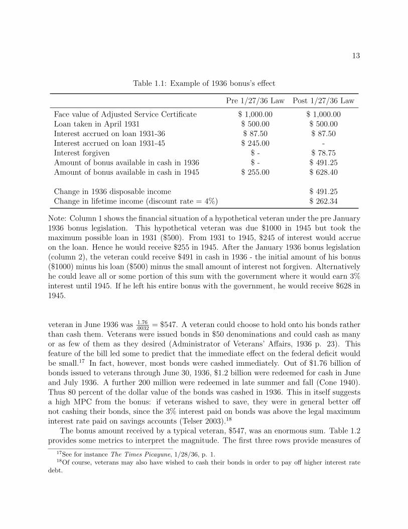
In June 1936, veterans received the entire face value of their bonus, less any loans they hadtaken. Thus they received a payment in 1936 equal to what they had been supposed toreceive in 1945. Importantly, interest accrued after October 1931 on loans taken againstthe bonus was forgiven (Administration of Veterans’ Affairs 1936). Table 1.1 illustrates theeffect of the law on a hypothetical veteran due $1000 in 1945 who took a loan of $500, themaximum allowable, in 1931. Such a veteran - who would have been typical - gained $491 ofdisposable income in 1936. The increment to the present value of a veteran’s total lifetimeincome was equal to the value of the loan interest forgiven plus the value of receiving theface value of the bonus in 1936 rather than in 1945. Assuming a discount rate of 4 percent,in this hypothetical case the change in present value total income was $262.

In June 1936, the government issued 1.76 billion of cashable bonds to 3.2 million veterans(Administrator of Veterans’ Affairs, 1936). Therefore the average value of the cashable bonds(i.e. the face value of his adjusted service certificate net of outstanding loans) received by a

16Most famously, Ernest Hemingway (1935), then a resident of Key West, wrote an op-ed entitled “WhoMurdered the Vets?: A First-Hand Report on the Florida Hurricane.”

13

Table 1.1: Example of 1936 bonus’s effect

Pre 1/27/36 Law Post 1/27/36 Law

Face value of Adjusted Service Certificate $ 1,000.00 $ 1,000.00Loan taken in April 1931 $ 500.00 $ 500.00Interest accrued on loan 1931-36 $ 87.50 $ 87.50Interest accrued on loan 1931-45 $ 245.00 -Interest forgiven $ - $ 78.75Amount of bonus available in cash in 1936 $ - $ 491.25Amount of bonus available in cash in 1945 $ 255.00 $ 628.40

Change in 1936 disposable income $ 491.25Change in lifetime income (discount rate = 4%) $ 262.34

Note: Column 1 shows the financial situation of a hypothetical veteran under the pre January1936 bonus legislation. This hypothetical veteran was due $1000 in 1945 but took themaximum possible loan in 1931 ($500). From 1931 to 1945, $245 of interest would accrueon the loan. Hence he would receive $255 in 1945. After the January 1936 bonus legislation(column 2), the veteran could receive $491 in cash in 1936 - the initial amount of his bonus($1000) minus his loan ($500) minus the small amount of interest not forgiven. Alternativelyhe could leave all or some portion of this sum with the government where it would earn 3%interest until 1945. If he left his entire bonus with the government, he would receive $628 in1945.

veteran in June 1936 was 1.76.0032

= $547. A veteran could choose to hold onto his bonds ratherthan cash them. Veterans were issued bonds in $50 denominations and could cash as manyor as few of them as they desired (Administrator of Veterans’ Affairs, 1936 p. 23). Thisfeature of the bill led some to predict that the immediate effect on the federal deficit wouldbe small.17 In fact, however, most bonds were cashed immediately. Out of $1.76 billion ofbonds issued to veterans through June 30, 1936, $1.2 billion were redeemed for cash in Juneand July 1936. A further 200 million were redeemed in late summer and fall (Cone 1940).Thus 80 percent of the dollar value of the bonds was cashed in 1936. This in itself suggestsa high MPC from the bonus: if veterans wished to save, they were in general better offnot cashing their bonds, since the 3% interest paid on bonds was above the legal maximuminterest rate paid on savings accounts (Telser 2003).18

The bonus amount received by a typical veteran, $547, was an enormous sum. Table 1.2provides some metrics to interpret the magnitude. The first three rows provide measures of

17See for instance The Times Picayune, 1/28/36, p. 1.18Of course, veterans may also have wished to cash their bonds in order to pay off higher interest rate

debt.

14

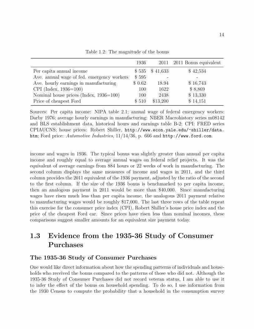
Table 1.2: The magnitude of the bonus

1936 2011 2011 Bonus equivalent

Per capita annual income $ 535 $ 41,633 $ 42,534Ave. annual wage of fed. emergency workers $ 595 - -Ave. hourly earnings in manufacturing $ 0.62 18.94 $ 16,743CPI (Index, 1936=100) 100 1622 $ 8,869Nominal house prices (Index, 1936=100) 100 2438 $ 13,330Price of cheapest Ford $ 510 $13,200 $ 14,151

Sources: Per capita income: NIPA table 2.1; annual wage of federal emergency workers:Darby 1976; average hourly earnings in manufacturing: NBER Macrohistory series m08142and BLS establishment data, historical hours and earnings table B-2; CPI: FRED seriesCPIAUCNS; house prices: Robert Shiller, http://www.econ.yale.edu/~shiller/data.

htm; Ford price: Automotive Industries, 11/14/36, p. 666 and http://www.ford.com.

income and wages in 1936. The typical bonus was slightly greater than annual per capitaincome and roughly equal to average annual wages on federal relief projects. It was theequivalent of average earnings from 884 hours or 22 weeks of work in manufacturing. Thesecond column displays the same measures of income and wages in 2011, and the thirdcolumn provides the 2011 equivalent of the 1936 payment, adjusted by the ratio of the secondto the first column. If the size of the 1936 bonus is benchmarked to per capita income,then an analogous payment in 2011 would be more than $40,000. Since manufacturingwages have risen much less than per capita income, the analogous 2011 payment relativeto manufacturing wages would be roughly $17,000. The last three rows of the table repeatthis exercise for the consumer price index (CPI), Robert Shiller’s house price index and theprice of the cheapest Ford car. Since prices have risen less than nominal incomes, thesecomparisons suggest smaller amounts for an equivalent size payment today.

1.3 Evidence from the 1935-36 Study of Consumer

Purchases

The 1935-36 Study of Consumer Purchases

One would like direct information about how the spending patterns of individuals and house-holds who received the bonus compared to the patterns of those who did not. Although the1935-36 Study of Consumer Purchases did not record veteran status, I am able to use itto infer the effect of the bonus on household spending. To do so, I use information fromthe 1930 Census to compute the probability that a household in the consumption survey

15

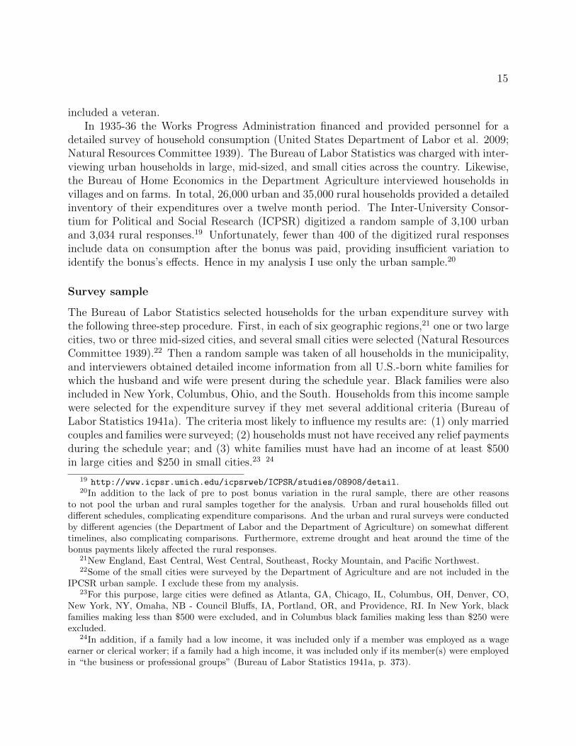
included a veteran.In 1935-36 the Works Progress Administration financed and provided personnel for a

detailed survey of household consumption (United States Department of Labor et al. 2009;Natural Resources Committee 1939). The Bureau of Labor Statistics was charged with inter-viewing urban households in large, mid-sized, and small cities across the country. Likewise,the Bureau of Home Economics in the Department Agriculture interviewed households invillages and on farms. In total, 26,000 urban and 35,000 rural households provided a detailedinventory of their expenditures over a twelve month period. The Inter-University Consor-tium for Political and Social Research (ICPSR) digitized a random sample of 3,100 urbanand 3,034 rural responses.19 Unfortunately, fewer than 400 of the digitized rural responsesinclude data on consumption after the bonus was paid, providing insufficient variation toidentify the bonus’s effects. Hence in my analysis I use only the urban sample.20

Survey sample

The Bureau of Labor Statistics selected households for the urban expenditure survey withthe following three-step procedure. First, in each of six geographic regions,21 one or two largecities, two or three mid-sized cities, and several small cities were selected (Natural ResourcesCommittee 1939).22 Then a random sample was taken of all households in the municipality,and interviewers obtained detailed income information from all U.S.-born white families forwhich the husband and wife were present during the schedule year. Black families were alsoincluded in New York, Columbus, Ohio, and the South. Households from this income samplewere selected for the expenditure survey if they met several additional criteria (Bureau ofLabor Statistics 1941a). The criteria most likely to influence my results are: (1) only marriedcouples and families were surveyed; (2) households must not have received any relief paymentsduring the schedule year; and (3) white families must have had an income of at least $500in large cities and $250 in small cities.23 24

19 http://www.icpsr.umich.edu/icpsrweb/ICPSR/studies/08908/detail.20In addition to the lack of pre to post bonus variation in the rural sample, there are other reasons

to not pool the urban and rural samples together for the analysis. Urban and rural households filled outdifferent schedules, complicating expenditure comparisons. And the urban and rural surveys were conductedby different agencies (the Department of Labor and the Department of Agriculture) on somewhat differenttimelines, also complicating comparisons. Furthermore, extreme drought and heat around the time of thebonus payments likely affected the rural responses.

21New England, East Central, West Central, Southeast, Rocky Mountain, and Pacific Northwest.22Some of the small cities were surveyed by the Department of Agriculture and are not included in the

IPCSR urban sample. I exclude these from my analysis.23For this purpose, large cities were defined as Atlanta, GA, Chicago, IL, Columbus, OH, Denver, CO,

New York, NY, Omaha, NB - Council Bluffs, IA, Portland, OR, and Providence, RI. In New York, blackfamilies making less than $500 were excluded, and in Columbus black families making less than $250 wereexcluded.

24In addition, if a family had a low income, it was included only if a member was employed as a wageearner or clerical worker; if a family had a high income, it was included only if its member(s) were employedin “the business or professional groups” (Bureau of Labor Statistics 1941a, p. 373).

16

Clearly the population sampled by the urban expenditure survey differed from that ofthe U.S. as a whole. Table 1.3 provides some indicators of how the urban expenditure samplecompares to the entire U.S. population. For comparison, the table also includes statistics onthe population of World War I veterans. The differences between the urban household surveysample and the U.S. population are an obvious consequence of the sampling procedures. Tothe extent that these differences were correlated with the size of a veteran’s bonus or withwhat a veteran did with his bonus, my results may not apply to the entire population ofveterans. A priori it is not obvious in which direction the composition of the urban householdsurvey might effect my measurement of the MPC. This is an issue to which I will returnwhen discussing my results.

Survey procedure

Households were interviewed over the course of 1936. In most cases, households were in-terviewed twice: once to obtain income information, and again to obtain expenditure in-formation. The interviews were typically about two months apart, although in some casesboth income and expenditure information were obtained in the same interview. Householdsgenerally reported on consumer expenditures over a 12 month period ending at the end ofthe month prior to the initial interview. Regardless of when they were first interviewed,however, households could choose to instead report income and expenditure for calendaryear 1935.25

The survey appears to have been carefully done. According to the Natural ResourcesCommittee (1939, p. 108):

The supervisory staffs in the regional administrative offices and in the local col-lection officies consisted of college graduates with training in the social sciences

There were other, noneconomic criteria for inclusion in the survey. In particular, according to the Bureauof Labor Statistics (1941a, p. 375) families were excluded from the expenditure survey if:

“

1. The family did not occupy a home in the community for at least 9 months of the scheduleyear.

2. The family moved from one dwelling unit to another between the end of the scheduleyear and the date of the interview.

3. The family did not have access to housekeeping facilities for at least 9 months of theschedule year.

4. The family had more than the equivalent of one roomer and/or boarder in the householdfor 52 weeks of the report year.

5. The family had more than the equivalent of one guest for 26 weeks.”

25One might worry that this is a source of bias if households interviewed after the bonus was paid selectedwhether or not to report on 1935 for reasons related to how they spent their bonus. In fact, results arequalitatively unchanged if one drops these households. See table 1.8.

17

Table 1.3: Sample characteristics

Population (%) Vets (%) 1935-36 hh survey (%)

Urban, 1930 45.8 56.4 100Married, if man age 30-50, 1930 80.3 77.7 100Black, 1930 9.7 6.8 6.6On relief, 1936 14.2 - 0Unemployment rate, 1936 10.0 - 0

Note: Urban is defined as living in a city of 10,800 or larger, since 10,800 is the smallest cityin the urban household survey.Sources: Data on the percent of the U.S. population and of World War I veterans thatlived in urban areas, was married, and or was black: IPUMS 5% sample of the 1930 census.Data on the number people living in households on relief comes from Chandler (1970, table11-2, column 3). I divide this by the U.S. population in 1936, taken from http://www.

census.gov/popest/data/national/totals/pre-1980/tables/popclockest.txt. Theunemployment rate is from Darby (1976, table 3, column 16).

and statistics, and in many cases with experience in the direction of surveys.The field agents and editors were selected from persons of clerical and profes-sional rating on Works Progress Administration rolls by mean of aptitude tests.. . .

As a further assurance of the accuracy of the data collected, a system of checkinterviewing was adopted, under the guidance of the regional office staffs. Ingeneral 1 out of every 8 or 10 families visited by each agent was revisited by asupervisor, editor, or squad leader, to check enough of the entries on the scheduleto prove that the agent had obtained the information from the family and hadreported it correctly.

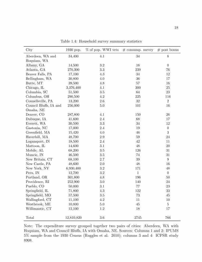
The appendix contains an example of a completed expenditure schedule, and provides adetailed description of how I compute measures of consumption aggregates from the surveyresponses. Table 1.4 provides summary statistics for the 33 cities included in the urban sam-ple.26 It provides information on city populations and the number of World War I veterans

26Although the IPCSR dataset has 3100 observations, the dataset I use has only 2745 observations. Idrop 34 households because they may have multiple veterans, 1 household because no city is specified, 37households because either the start or end data for the schedule year is missing, 3 households because theschedule period is under a year, 20 households because the schedule period is over a year, 18 householdsbecause there is a discrepancy between the schedule year listed on the household’s income schedule and theschedule year listed on the expenditure schedule, 2 households because the husband is listed as being underage 16, 11 households because the husband’s age is missing, and 229 households because the husband’s raceis unknown.

18

Table 1.4: Household survey summary statistics

City 1930 pop. % of pop. WWI vets # consump. survey # post bonus

Aberdeen, WA and 34,400 4.1 34 8Hoquiam, WAAlbany, GA 14,500 3.2 16 0Atlanta, GA 270,300 3.3 239 76Beaver Falls, PA 17,100 4.3 34 12Bellingham, WA 30,800 4.0 36 17Butte, MT 39,500 4.8 57 16Chicago, IL 3,376,400 4.1 300 25Columbia, SC 51,500 3.5 64 23Columbus, OH 290,500 4.2 225 116Connellsville, PA 13,200 2.6 32 2Council Bluffs, IA and 256,000 5.0 101 16Omaha, NEDenver, CO 287,800 4.1 150 26Dubuque, IA 41,600 2.4 68 17Everett, WA 30,500 3.3 34 12Gastonia, NC 17,000 2.4 19 0Greenfield, MA 15,420 4.0 46 3Haverhill, MA 48,700 2.9 59 24Logansport, IN 18,500 2.4 42 11Mattoon, IL 14,600 3.1 48 20Mobile, AL 68,200 3.5 126 31Muncie, IN 46,500 3.5 74 31New Britain, CT 68,100 2.7 39 9New Castle, PA 48,600 2.0 48 16New York, NY 6,930,400 3.2 171 48Peru, IN 12,700 3.2 1 0Portland, OR 301,800 4.8 196 50Providence, RI 252,900 3.0 140 24Pueblo, CO 50,000 3.1 77 23Springfield, IL 71,800 4.3 122 33Springfield, MO 57,500 3.5 73 45Wallingford, CT 11,100 4.2 11 10Westbrook, ME 10,800 5.0 45 5Willimantic, CT 12,100 1.2 18 17

Total 12,810,820 3.6 2745 766

Note: The expenditure survey grouped together two pairs of cities: Aberdeen, WA withHoquiam, WA and Council Bluffs, IA with Omaha, NE. Sources: Columns 1 and 2: IPUMS5% sample from the 1930 Census (Ruggles et al. 2010); columns 3 and 4: ICPSR study8908.

19

Table 1.5: Consumption category summary statistics

Category Mean ($’s) Standard deviation ($’s)

Total expenditure 1870 1217Auto purchases and operations 183 263Housing 232 267Furniture and equipment 55 102Clothing 205 195Recreation 73 136Food 583 278

Source: ICPSR study 8908. For details on these consumption categories see the appendix.

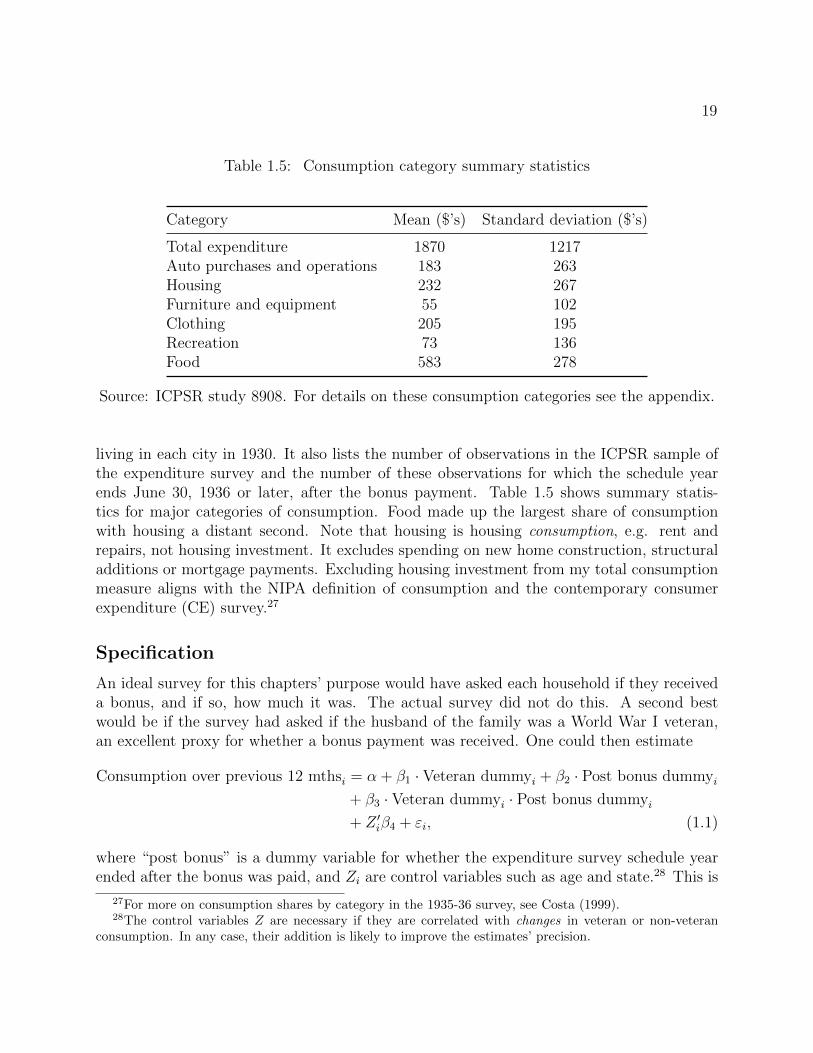
living in each city in 1930. It also lists the number of observations in the ICPSR sample ofthe expenditure survey and the number of these observations for which the schedule yearends June 30, 1936 or later, after the bonus payment. Table 1.5 shows summary statis-tics for major categories of consumption. Food made up the largest share of consumptionwith housing a distant second. Note that housing is housing consumption, e.g. rent andrepairs, not housing investment. It excludes spending on new home construction, structuraladditions or mortgage payments. Excluding housing investment from my total consumptionmeasure aligns with the NIPA definition of consumption and the contemporary consumerexpenditure (CE) survey.27

Specification

An ideal survey for this chapters’ purpose would have asked each household if they receiveda bonus, and if so, how much it was. The actual survey did not do this. A second bestwould be if the survey had asked if the husband of the family was a World War I veteran,an excellent proxy for whether a bonus payment was received. One could then estimate

Consumption over previous 12 mthsi = α + β1 · Veteran dummyi + β2 · Post bonus dummyi

+ β3 · Veteran dummyi · Post bonus dummyi

+ Z ′iβ4 + εi, (1.1)

where “post bonus” is a dummy variable for whether the expenditure survey schedule yearended after the bonus was paid, and Zi are control variables such as age and state.28 This is

27For more on consumption shares by category in the 1935-36 survey, see Costa (1999).28The control variables Z are necessary if they are correlated with changes in veteran or non-veteran

consumption. In any case, their addition is likely to improve the estimates’ precision.

20

a standard differences in differences regression with β3 measuring the difference between thechange in veteran consumption pre to post bonus and the change in non-veteran consumptionpre to post bonus. Any changes to consumption common to both veterans and non-veteranswill be differenced out and will not be reflected in β3.29 Along with a reasonable estimateof the size of the average bonus, an estimate of β3 will provide an estimate of veterans’propensity to consume out of the bonus.

Although the survey did not ask about veteran status, it is still possible to identify β3.To do so, I proxy for veteran status with a measure of the probability that the husband ina household was a veteran. I take advantage of the fact that the household survey includesinformation on age, race, and location. Since the 1930 census asked everyone if they werea World War I veteran, I can use the IPUMS 5% sample from this census to estimate theprobability that a household contains a veteran conditional on age, race, and location. Thisprobability then replaces the veteran dummy in equation 1.1. Thus the estimation equationis

Consumptioni = α + β1 · Prob. veterani + β2 · Post bonus dummyi

+ β3 · Prob. veterani · Post bonus dummyi + Z ′iβ4 + εi, (1.2)

The procedure is similar to the two-sample instrumental variables approach described inAngrist and Krueger (1992), Lusardi (1996), and Inoue and Solon (2010), although it differsin important ways. Most obviously, I resort to a two-sample procedure not because veteranstatus is endogenous, but because I do not observe it in the first sample.30 Let Y be theoutcome variable of interest, consumption, X be veteran status, and Z a vector of covariatescorrelated with X. In the typical two-sample instrumental variables problem Y and Z areobserved in one-sample (in my case the household survey) and X and Z are observed ina second sample (in my case the 1930 census). Under the same assumptions needed forsingle-sample IV estimation, β = (X ′X)−1X ′Y is a consistent estimator of β, where X arethe predicted values for X from the least-squares regression of X on Z in the second sample.

My problem differs from the above in that I am interested in identifying the effect onconsumption of veteran status interacted with the post bonus dummy, not the effect ofveteran status on consumption. Thus if P is the post bonus dummy, the required exclusionrestriction is not that E[εZ] = 0 but that E[ε(Z · P )] = 0. To see this write the first stageregression

Xj = Z ′jγ + µj, (1.3)

and the second stage regression

Yi = α + (Z ′iγ)β1 + Piβ2 + ((Z ′iγ)Pi)β3 + Z ′iβ4 + (Z ′iPi)β5 + εi. (1.4)

29Thus the existence of spillover (multiplier) effects from the bonus will not bias an estimate of β3. Thatis, as long as spillovers from the bonus affected veteran and non-veterans equally.

30Card and McCall (1996) use a two-sample procedure for similar reasons. They wish to measure theeffect of medical insurance coverage on worker compensation claims for Monday injuries, but they do notobserve insurance coverage in their sample of injury claims.

21

Estimating 1.4 is equivalent to estimating

Yi = α + Z ′i(β1γ + β4) + Piβ2 + (Z ′iPi)(β3γ + β5) + εi. (1.5)

It is thus possible to identify α

β1γ + β4

β2

β3γ + β5

Given γ, β3 is identifiable if and only if β5 = 0. The variables used to predict veteran sta-

tus must be uncorrelated with the pre to post bonus change in consumption except throughveteran status. For example, while it poses no problem for identification of the MPC if raceis correlated with consumption for reasons other than veteran status, it will bias my esti-mates if for reasons other than veteran status race is correlated with the pre to post bonuschange in consumption. As the analogy with instrumental variables suggests, conditionalon the exclusion restriction holding, estimation of (1.3) and (1.4) by least squares providesconsistent coefficient estimates. The appendix sketches a proof and provides more discussionof the necessary assumptions.

Since Ziγ, the probability of being a veteran, is a generated regressor, the usual formulaswill underestimate standard errors. Further complicating the calculation of correct standarderrors, the household survey data is from a stratified sample. Each primary sampling unit - acity - was drawn from 15 region-city-size strata. To avoid problems with strata that containonly one primary sampling unit, I collapse the 15 strata to 9. The appendix providesdetails. To account for the generated regressor problem, possible correlation of standarderrors within cities (clustering), and the stratified survey design, I compute block bootstrapstandard errors.31

31Specifically, I repeat the following 1000 times:

1. Draw a bootstrap sample (i.e. a sample with replacement) of cities from each of the 9 strata in thehousehold survey. For example, since one stratum is large cities in the east central region, the samplemight have Chicago and Columbus, OH, or two instances of Chicago and no Columbus, OH. But itwill for certain have at least one large city from the east central region.

2. Estimate the probability of being a veteran conditional on age, race, and location (γ) on this bootstrapsample.

3. Estimate the equation of interest (1.2).

4. Save the coefficients.

The standard error is then the standard deviation of these 1000 coefficient estimates.

22

Results

In the first stage regression I estimate the linear probability model of World War I veteranstatus on a set of age, race, and state fixed effects.32 Specifically, I estimate:33

Vj =3∑

h=1

βh1(gj = gh) +17∑k=1

γk1(sj = sk) +17∑l=1

αl1(gj = 2)1(sj = sl)

+3∑

m=1

θmamj +

3∑n=1

λn1(gj = 2)anj + ζrj + η1(gj = 2) · rj + µj. (1.6)

Variables are defined as follows: V is World war I veteran status; g is a generation indicatorvariable for whether a man was younger than 28, between 28 and 45 or older than 45 in 1930(men younger than 28 or older than 45 had less than a 4 percent chance of being a veteran);s is an indicator variable for state; a equals age, and r is an indicator variable for race.1 denotes the indicator function. The predicted probabilities of being a veteran are fairlyinsensitive to the exact specification used, and my estimates of the MPC will be consistentregardless of whether the first stage is misspecified.34 The particular specification in (1.6) isattractive because while fairly parsimonious, it results in separate slope coefficients for menage 28 to 45, the age range in which men had a reasonable chance of having served in thewar.

The first stage estimation is done on a sample from the 1930 Census that approximatesthe household survey as closely as possible. Thus I use the IPUMS 5 percent sample fromthe 1930 census for all U.S. born men married to U.S. born women in the 33 cities includedin the urban portion of the household survey. This provides me with 64,144 observations,enough to precisely estimate the probability of being a veteran as a function of age, race,and location. The first stage produces large variation in the probability that the husband inthe household was a veteran.35 Table 1.6 gives some examples of how this probability varieswith age, race and location.

In the second step, I estimate equation 1.2, where consumption is the dependent variable.Table 1.7 shows results for total consumption expenditure.36 The specification in column 1 oftable 1.7 uses all observations. Column 2, my preferred specification, excludes households in

32Although it would undoubtedly produce more accurate estimates of the probability that a man was aveteran, using probit or logit in the first stage would be problematic since the first stage residuals would nolonger be uncorrelated with the first stage regressors (an example of what’s known as ‘forbidden regression’).For details, see the appendix.

33In stata notation the right-hand side variables are “young old i.elig#i.race i.elig#i.state i.elig#c.agei.elig#c.age2 i.elig#c.age3” where elig = 1 - young - old.

34See the proof in the appendix. As in the IV context, the key assumption is that the errors fromthe first stage are uncorrelated with the regressors - something that OLS guarantees is true regardless ofmisspecification.

35The first stage R2 is 0.21. Most of the variation comes from age, rather than race or location. Seetable 1.8.

36The appendix describes exactly what is included in this aggregate.

23

Table 1.6: Variation in probability man is a veteran

Age in 1936 Race City Prob. vet

35 White Bellingham, WA 0.2035 White Chicago, IL 0.1735 White Denver, CO 0.1835 White Atlanta, GA 0.1335 Black Atlanta, GA 0.0438 White Bellingham, WA 0.4638 White Chicago, IL 0.4438 White Denver, CO 0.4538 White Atlanta, GA 0.3938 Black Atlanta, GA 0.30

the consumer expenditure survey with total spending of more than $5000. These householdsare large outliers in the regression: a robust regression assigns them approximately zeroweight. In each specification, two coefficients are shown: that on the post bonus dummy,and that on the interaction term between the post bonus dummy and the probability ofbeing a veteran. No results are shown for the probability of being a veteran itself, since thisis simply a linear combination of the controls. One might initially be concerned that thecoefficient on the post bonus dummy is large and statistically significant, since this suggeststhat non-veteran as well as veteran spending changed pre to post bonus. But this is infact exactly what one would expect given the upward trend in aggregate consumption overthis period. Furthermore, if non-veterans also benefited from the bonus, i.e. if there was amultiplier, than even absent trend consumption growth one would expect to see an increasein their consumption after the bonus payment.37

To interpret the coefficient on the interaction, recall that average household expenditurein the sample was $1870 (table 1.5), and that the average bonus received by a World War Iveteran was $547. If it were the case that the average bonus paid to veterans in the samplewas the same as that in the population as a whole, then the coefficient in column 2 wouldimply a MPC of 0.74 ($403 / $547). However, the average bonus in the urban householdsurvey population may have differed from that in the population as a whole.

Three factors were important in determining what size bonus a veteran received. (1)How many days a veteran served in the army; (2) whether those days were served in theU.S. or abroad, and (3) what size loan, if any, the veteran had taken against his bonus.Unfortunately, there is no direct information available about how any of these factors varied

37The magnitude of the coefficient on the post bonus dummy in column 2, 198, implies approximately a10-15 percent increase in nonveteran consumption pre to post bonus. While not directly comparable, thisis roughly in line with the NIPA data which shows aggregate consumption rising by 10.2 percent in 1936(NIPA table 1.1.1).

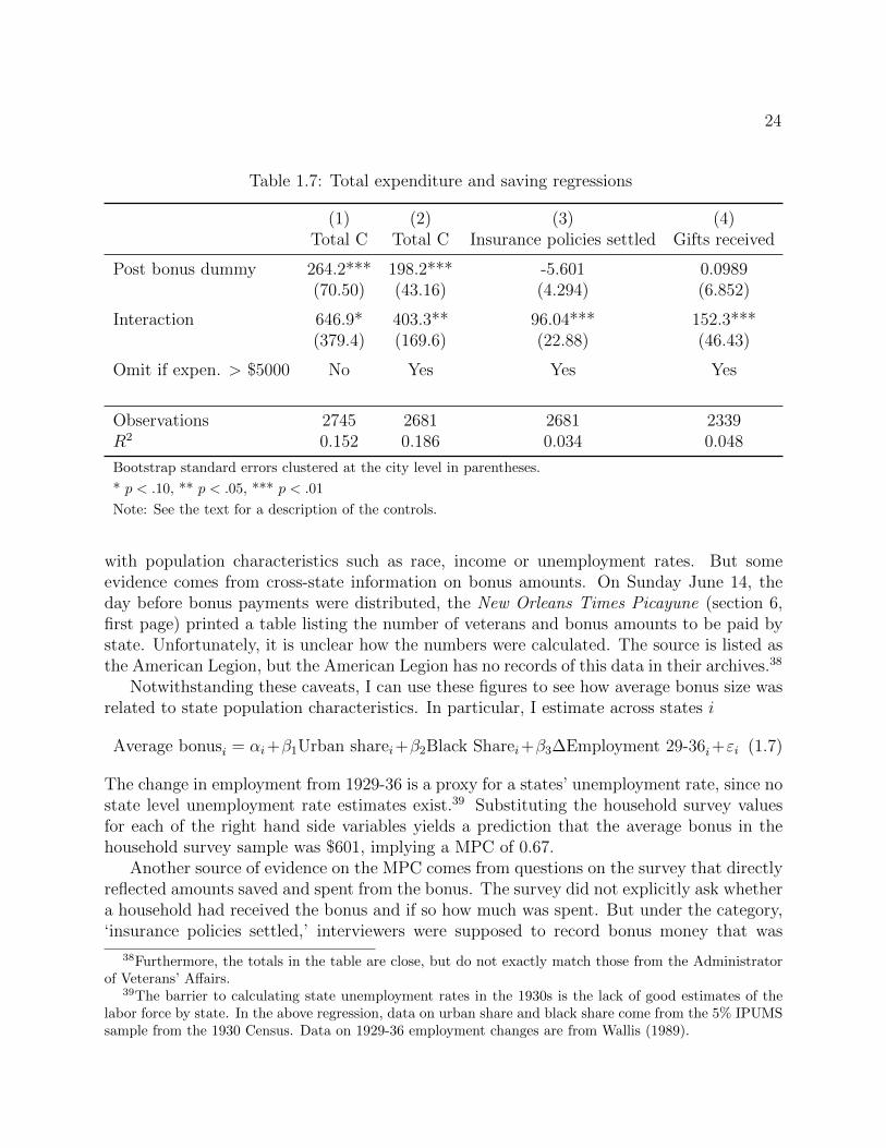
24

Table 1.7: Total expenditure and saving regressions

(1) (2) (3) (4)Total C Total C Insurance policies settled Gifts received

Post bonus dummy 264.2*** 198.2*** -5.601 0.0989(70.50) (43.16) (4.294) (6.852)

Interaction 646.9* 403.3** 96.04*** 152.3***(379.4) (169.6) (22.88) (46.43)

Omit if expen. > $5000 No Yes Yes Yes

Observations 2745 2681 2681 2339R2 0.152 0.186 0.034 0.048

Bootstrap standard errors clustered at the city level in parentheses.

* p < .10, ** p < .05, *** p < .01

Note: See the text for a description of the controls.

with population characteristics such as race, income or unemployment rates. But someevidence comes from cross-state information on bonus amounts. On Sunday June 14, theday before bonus payments were distributed, the New Orleans Times Picayune (section 6,first page) printed a table listing the number of veterans and bonus amounts to be paid bystate. Unfortunately, it is unclear how the numbers were calculated. The source is listed asthe American Legion, but the American Legion has no records of this data in their archives.38

Notwithstanding these caveats, I can use these figures to see how average bonus size wasrelated to state population characteristics. In particular, I estimate across states i

Average bonusi = αi+β1Urban sharei+β2Black Sharei+β3∆Employment 29-36i+εi (1.7)

The change in employment from 1929-36 is a proxy for a states’ unemployment rate, since nostate level unemployment rate estimates exist.39 Substituting the household survey valuesfor each of the right hand side variables yields a prediction that the average bonus in thehousehold survey sample was $601, implying a MPC of 0.67.

Another source of evidence on the MPC comes from questions on the survey that directlyreflected amounts saved and spent from the bonus. The survey did not explicitly ask whethera household had received the bonus and if so how much was spent. But under the category,‘insurance policies settled,’ interviewers were supposed to record bonus money that was

38Furthermore, the totals in the table are close, but do not exactly match those from the Administratorof Veterans’ Affairs.

39The barrier to calculating state unemployment rates in the 1930s is the lack of good estimates of thelabor force by state. In the above regression, data on urban share and black share come from the 5% IPUMSsample from the 1930 Census. Data on 1929-36 employment changes are from Wallis (1989).

25

received but not spent.40 Column 3 of table 1.7 replicates the specification in column 2,but with this variable rather than total spending as the dependent variable. The coefficientimplies that the average veteran in the survey saved $96 of his bonus. This coefficient must,however, be interpreted with caution, since there was probably a problem of non-responseson the insurance-policies-settled question. (It may not have been intuitive that there is whereone was supposed to state the amount of a bonus not spent.) Hence, the coefficient mayunderestimate how much veterans actually saved.

In the initial interview (usually about two months before the expenditure survey inter-view), households were also asked about the value of “Gifts in cash for current use frompersons not members of economic family.”41 Interviewers were supposed to record here theamount of the bonus spent on consumption. As with the saving question, one suspects thatmany did not. Column 4 shows results for this variable. As expected, the coefficient onthe interaction term is highly significant. Not surprisingly, the sum of this coefficient withthat for the measure of bonus saving (column 3) implies an implausibly low average bonusamount of $152+$96 = $248. This is as expected if many respondents mistakenly enteredzero. Still, assuming that the measurement error for the two measures was similar, the ratio

$152$96+$152

= 0.61 provides an alternative estimate of the MPC.The preponderance of evidence thus suggests that the MPC was between 0.6 and 0.75. As

the forgoing discussion indicates, it is difficult to say more precisely what the MPC was. Inaddition to uncertainty about the exact bonus amount received by veterans in the householdsurvey, there is also reason to doubt that the MPC of veterans in the survey was identicalto that of veterans as a whole. Since veterans as whole were more likely to be poor andunemployed, it seems likely that the MPC as measured in the household survey is biaseddown. This would be the case if unemployed veterans - who do not show up in the householdsurvey - were hand-to-mouth consumers who spent their entire bonus. In any case, as weshall see, a MPC in this range fits well with evidence from alternative specifications, andfrom other, independent sources of data.

40According to the BLS (1941b, p. 15):

Some families which furnished expenditure schedules received money during the schedule yearfrom cash gifts, inheritances, or the soldiers’ bonus. That part of such receipts which was usedfor current living expenses was treated as current money income. The remainder was eithersaved or invested, and was thus represented by an increase in one or another appropriate item–savings accounts, real estate, or the like. To balance such increases, a decrease was enteredunder “Other assets” in the case of cash gifts or inheritance and under “Insurance policiessettled” in the case of the soldiers’ bonus.

Note that this variable could be non-zero even if one did not receive a bonus. This was where the interviewerwas supposed to record the payout from any insurance policies held by the household.

41See the urban family schedule in the ICPSR documentation for study 8908 and BLS (1939) p. 196.

26

Robustness

Table 1.8 shows several robustness checks for the baseline total expenditure specification.For comparison, column 1 reproduces column 2 of table 1.7, my preferred specification. Oneconcern about this specification is that the exclusion restriction may be violated if cities havedifferent seasonal consumption patterns. Suppose that, for example, cities in the north havemore veterans and always consume more in fall than in spring. Then my estimation strategywould ascribe part of this increase in consumption from spring to fall to higher proportionsof veterans in these cities, and hence would overestimate the MPC from the bonus. Column2 of table 1.8 tests for this possibility by using only age and race, not geography, to predictveteran probability in the first stage. In fact, this results in a larger estimate of the spendingresponse. As one can see from comparing the first stage R2s, dropping geographic controlsresults in little loss of explanatory power for the probability of being a veteran. Most ofthe difference in the second stage coefficient is instead driven by the fact that without statefixed effects in the first stage, one must also drop state fixed effects from the second stage.42

If one ignores the econometric issues and still includes state fixed effects, the coefficient incolumn 2 is 446, much closer to that in column 1.

One might also be concerned that different time patterns of consumption between whitesand blacks could bias my coefficient. Hence in column 3, I use only age to predict veteranstatus. The point estimate again rises, and again this increase is driven primarily not bedifferent estimates of the probability of being a veteran but by the change in the secondstage control variables.43 As a further check for the effect of race on my results, in column4 I perform both the first and second stage estimation for whites only. The coefficient isessentially unchanged from that in column 1. Column 5 restricts the first stage sample tomen who are employed in 1930. Since the 1936 household survey included only employedmen, it would be a concern if the relationship between the covariates and veteran statuswere different for the employed and the unemployed.44 In practice, this does not appear tobe concern: the coefficient on the interaction in column 5 is essentially identical to that incolumn 1.

Finally, one might worry that the ability of households to choose to report on calendaryear 1935 rather than the most recent 12 month period is a source of bias. Suppose, forinstance, that veterans who spent much of their bonus were less likely to report on 1935.This could be because households were eager to report recent salient purchases. In this case,the coefficient would be biased up: I would observe more spending among veterans postbonus than actually occurred. To see if this effect is driving my results, in column 6 I drop

42One cannot include variables in the second stage that are not in the first stage and have a consistentestimator, since consistency requires that the first stage residuals be uncorrelated with the second stage righthand side variables. See the appendix.

43If one were to ignore the econometric problems and includes the baseline controls, the coefficient incolumn 3 would be 437.

44Of course, veterans who were unemployed in 1930 were different people from those unemployed in 1936.This is why in my baseline specification I do not drop those who were unemployed in 1930 from the firststage.

27

Table 1.8: Total expenditure robustness checks

(1) (2) (3) (4) (5) (6)Baseline Age, race only Age only White only Emp. only Post, rpt. ’35

Post bonus 198.2*** 117.5*** 80.81* 205.2*** 199.3*** 199.9***(43.16) (44.50) (44.18) (45.28) (41.08) (50.01)

Interaction 403.3** 520.9*** 662.8*** 380.1** 395.5** 460.4**(169.6) (159.4) (181.0) (178.5) (168.6) (204.7)

1st stage N 64,144 64,144 64,144 57,699 57,390 64,1442nd stage N 2681 2681 2681 2501 2681 20731st stage R2 0.213 0.212 0.209 0.220 0.214 0.2132nd stage R2 0.186 0.136 0.054 0.110 0.186 0.205

Bootstrap standard errors clustered at the city level in parentheses

* p < .10, ** p < .05, *** p < .01

Notes: See the text for a description of the controls.

Households with total expenditure > $5000 are excluded.

all households interviewed after the bonus was paid (i.e. after 6/15/36) who chose to reporton 1935. The measured MPC actually rises slightly.

Overall these robustness tests are reassuring; they suggest that the results are not drivenby a particular specification or sample. If anything, my baseline results appear conservative:other specifications often yield higher point estimates. Nonetheless, any one dataset andestimation strategy inevitably comes with uncertainties. This motivates identifying alterna-tive, independent sources of evidence on the bonus’s effects. I turn to these in the followingsections. But first I use the household survey to see what veterans bought with their bonus.

Expenditure categories

The detail of the household survey allows me to break down the spending response acrossconsumption categories. Table 1.9 reproduces for several categories of consumption thebaseline specification that excludes households with spending greater than $5000.45 Thefirst column reports results for total automobiles-related spending, including new and usedcar purchases, gasoline and repairs. The coefficient is economically and statistically highlysignificant. It implies that roughly one-third of the total spending response was in thisconsumption category. Column 2 shows results for housing. This is housing consumption(rent and repairs), not residential investment, so it excludes house purchases and structuraladditions. Still, results suggest a large effect of the bonus. The coefficients for the remainingcategories of consumption imply economically nontrivial amounts of spending but are lessprecisely estimated.

45As argued above, these households are large outliers.

28

Tab

le1.

9:C

onsu

mpti

onca

tego

ryre

gres

sion

s

(1)

(2)

(3)

(4)

(5)

(6)

Auto

purc

has

esan

dop

s.H

ousi

ng

Furn

iture

/eq

uip

men

tC

loth

ing

Rec

reat

ion

Food

Pos

tb

onus

dum

my

47.7

7***

9.51

64.

952

41.4

7***

9.32

3***

29.9

3**

(10.

77)

(8.4

25)

(5.2

44)

(7.7

33)

(3.1

31)

(12.

76)

Inte

ract

ion

127.

5**

83.2

8***

21.7

232

.99

24.8

935

.16

(60.

29)

(29.

40)

(20.

44)

(27.

08)

(15.

76)

(45.

66)

Obse

rvat

ions

2681

2681

2681

2681

2681

2681

R2

0.07

20.

204

0.05

10.

091

0.07

40.

231

Boot

stra

pst

and

ard

erro

rscl

ust

ered

atth

eci

tyle

vel

inp

are

nth

eses

*p<.1

0,**

p<.0

5,**

*p<.0

1

Not

es:

See

the

text

for

ad

escr

ipti

onof

the

contr

ols

.H

ou

seh

old

sw

ith

tota

lex

pen

dit

ure>

$5000

are

excl

ud

ed.

‘op

s.’

mea

ns

op

erati

on

s.

Tab

le1.

10:

Auto

sre

gres

sion

s

(1)

(2)

(3)

(4)

Auto

purc

has

esan

dop

s.A

uto

purc

has

esC

arpurc

has

eA

uto

oper

atio

ns

Pos

tb

onus

dum

my

47.7

7***

28.2

6***

0.00

387

19.5

1***

(10.

77)

(7.6

85)

(0.0

146)

(6.9

02)

Inte

ract

ion

127.

5**

71.0

4*0.

215*

**56

.45*

(60.

29)

(37.

89)

(0.0

750)

(30.

11)

Obse

rvat

ions

2681

2681

2681

2681

R2

0.07

20.

039

0.04

70.

075

Boot

stra

pst

and

ard

erro

rscl

ust

ered

at

the

city

level

inp

are

nth

eses

*p<.1

0,**

p<.0

5,**

*p<.0

1

Not

es:

See

the

text

for

ad

escr

ipti

on

of

the

contr

ols

.H

ou

seh

old

sw

ith

tota

lex

pen

dit

ure>

$5000

are

excl

ud

ed.

29

Because of its importance for the overall spending response, table 1.10 looks in more detailat the response of autos consumption to the bonus payments. For comparison, column 1reproduces column 1 of table 1.9. In column 2, the dependent variable is money spent onauto purchases (new and used) only. The result suggests that more than half the autosspending response came from car purchases.46 The third column shows results from thelinear probability model in which the left hand side variable is a dummy corresponding towhether or not a household purchased a car in the schedule year. The coefficient implies thatthe bonus increased the probability of a car purchase by 22 percentage points. This is large:in the sample as a whole, the probability that a household bought a car was 19 percent.The final column of table 1.10 shows the response of all auto-related spending except carpurchases. This includes gasoline, repairs, and purchases such as tires and car radios. Theresponse is large, suggesting that even veterans who did not purchase a car responded to thebonus by investing in existing cars and / or driving more.

1.4 Cross-state and cross-city evidence

Another source of evidence on the bonus’s effects comes from cross-state and cross-cityregressions. States and cities varied in the proportion of their population made up of veterans,and hence in the amount of stimulus they received. Thus by relating variation across statesand cities in veterans per capita with state or city level data on economic outcomes, it ispossible to make inferences about the effects of the bonus.

The Geographic Distribution of Veterans

Veterans were unevenly distributed across the U.S. Figure 1.1 shows data from the 1930Census on the percent of each state’s population made up of World War I veterans.47 Thereis large geographic variation, from a low of 1.8 veterans per 100 people in Mississippi toa high of 5.2 veterans per 100 people in Wyoming, the District of Columbia, and Nevada.States in the south tended to have fewer veterans while states west of the Mississippi tendedto have more.

Two forces combined to lower the share of veterans in the south. First, blacks were lesslikely than whites to have served in World War I. In 1930, 2.1 percent of blacks were veterans,whereas 3.1 percent of whites were veterans.48 Since black populations were much larger inthe south, this mechanically led to lower overall shares of veterans in the population. This isnot, however, the entire explanation for the low share of veterans in the former Confederacy.

46It would be natural to estimate the response of car purchases with a tobit rather than a linear model.Indeed, measurement of household auto purchases is the example Tobin (1958) uses to motivate his estimator.However, my two-step procedure provides consistent estimates only if the second stage is linear. Thisreasoning is also why I estimate a linear probability model rather than a probit in column 3.

47Data are from the IPUMS 5 percent sample of the 1930 Census (Ruggles et al. 2010).48Figures cited in this paragraph were computed from the IPUMS 5 percent sample of the 1930 Census.

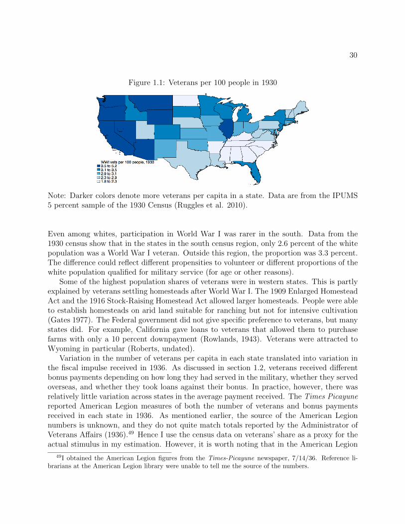
30

Figure 1.1: Veterans per 100 people in 1930

Note: Darker colors denote more veterans per capita in a state. Data are from the IPUMS5 percent sample of the 1930 Census (Ruggles et al. 2010).

Even among whites, participation in World War I was rarer in the south. Data from the1930 census show that in the states in the south census region, only 2.6 percent of the whitepopulation was a World War I veteran. Outside this region, the proportion was 3.3 percent.The difference could reflect different propensities to volunteer or different proportions of thewhite population qualified for military service (for age or other reasons).

Some of the highest population shares of veterans were in western states. This is partlyexplained by veterans settling homesteads after World War I. The 1909 Enlarged HomesteadAct and the 1916 Stock-Raising Homestead Act allowed larger homesteads. People were ableto establish homesteads on arid land suitable for ranching but not for intensive cultivation(Gates 1977). The Federal government did not give specific preference to veterans, but manystates did. For example, California gave loans to veterans that allowed them to purchasefarms with only a 10 percent downpayment (Rowlands, 1943). Veterans were attracted toWyoming in particular (Roberts, undated).

Variation in the number of veterans per capita in each state translated into variation inthe fiscal impulse received in 1936. As discussed in section 1.2, veterans received differentbonus payments depending on how long they had served in the military, whether they servedoverseas, and whether they took loans against their bonus. In practice, however, there wasrelatively little variation across states in the average payment received. The Times Picayunereported American Legion measures of both the number of veterans and bonus paymentsreceived in each state in 1936. As mentioned earlier, the source of the American Legionnumbers is unknown, and they do not quite match totals reported by the Administrator ofVeterans Affairs (1936).49 Hence I use the census data on veterans’ share as a proxy for theactual stimulus in my estimation. However, it is worth noting that in the American Legion

49I obtained the American Legion figures from the Times-Picayune newspaper, 7/14/36. Reference li-brarians at the American Legion library were unable to tell me the source of the numbers.

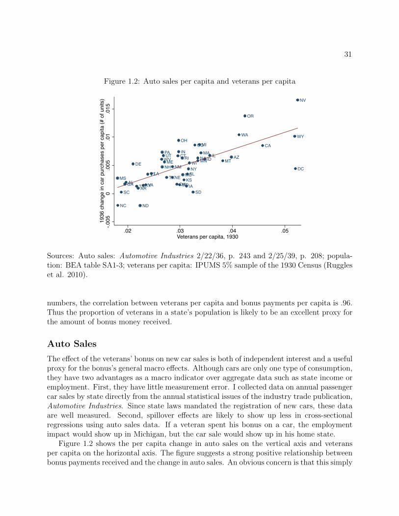
31

Figure 1.2: Auto sales per capita and veterans per capita

AL

AZ

AR

CACO

CT

DEDC

FL

GA

IDIL

IN

IAKS

KY

LA

ME

MD

MA

MI

MN

MSMO

MT

NE

NV

NH

NJ

NM NY

NC ND

OH

OK

OR

PARI

SC SDTN

TX

UT

VT

VA

WA

WVWI

WY

-.005

0.0

05.0

1.0

1519

36 c

hang

e in

car

pur

chas

es p

er c

apita

(# o

f uni

ts)

.02 .03 .04 .05Veterans per capita, 1930

Sources: Auto sales: Automotive Industries 2/22/36, p. 243 and 2/25/39, p. 208; popula-tion: BEA table SA1-3; veterans per capita: IPUMS 5% sample of the 1930 Census (Ruggleset al. 2010).

numbers, the correlation between veterans per capita and bonus payments per capita is .96.Thus the proportion of veterans in a state’s population is likely to be an excellent proxy forthe amount of bonus money received.

Auto Sales

The effect of the veterans’ bonus on new car sales is both of independent interest and a usefulproxy for the bonus’s general macro effects. Although cars are only one type of consumption,they have two advantages as a macro indicator over aggregate data such as state income oremployment. First, they have little measurement error. I collected data on annual passengercar sales by state directly from the annual statistical issues of the industry trade publication,Automotive Industries. Since state laws mandated the registration of new cars, these dataare well measured. Second, spillover effects are likely to show up less in cross-sectionalregressions using auto sales data. If a veteran spent his bonus on a car, the employmentimpact would show up in Michigan, but the car sale would show up in his home state.

Figure 1.2 shows the per capita change in auto sales on the vertical axis and veteransper capita on the horizontal axis. The figure suggests a strong positive relationship betweenbonus payments received and the change in auto sales. An obvious concern is that this simply

32

reflects a correlation between veteran population in a state and some other factor drivingauto sales growth. For instance, veterans per capita could be correlated with agriculturalincome, given the prevalence of veterans in the west. I address this concern in three ways:first, by estimating regressions with a variety of control variables, second, by estimatingregressions on subsets of states, and finally, by running placebo tests to see if the presenceof veterans is correlated with auto sales in other years of the 1930s.

Regression results are shown in table 1.11. The first column shows estimates from thesimple regression analogous to the scatter plot. Column 2 controls for the level of per capitanew car sales in 1929, the interwar era sales peak. Per capita sales in 1929 had regionalvariation that was correlated with that of veterans per capita: auto sales were higher inthe sparsely populated west than they were in the east or south. However, adding thiscontrol to the regression has almost no effect on the coefficient (column 2). Results are alsolittle changed when one controls for the lagged change in car sales per capita (column 3).The above discussion of the geographic distribution of veterans and its causes suggests it isimportant to control for region fixed effects, or the share of a state’s population living onfarms and the share of a state’s population that was black. This is done in columns 4 and 5.While the size of the coefficient on veterans per capita falls, it remains highly statisticallysignificant. The last two columns of the table return to the simple regression of the change inauto sales on veteran share, but restrict the sample of states. Column 6 drops the five stateswith fewer than two veterans per capita (Alabama, Georgia, Mississippi, North Carolina,and South Carolina) and the six states with more than four veterans per capita (California,Nevada, Oregon, Washington, Washington, DC, and Wyoming). The sample is limited incolumn 7 to the 21 states in the midwest and northeast. In both cases, the coefficient onveterans per capita is little changed from that in column 1, although when the sample sizeis cut to 21, the standard error is unsurprisingly larger.

The estimates in table 1.11 suggest that the coefficient on veterans per capita lies between0.2 and 0.35. This means that for every additional veteran living in a state, 0.2 to 0.35 morenew cars were sold in 1936. The average retail price of a car in 1936 was $781 (Suits 1958),thus if veterans bought average-priced cars, then an additional veteran increased new carspending by roughly $200. Of course, it is likely that veterans tended to buy lower pricecars that could be afforded with a bonus check. If, for example, veterans only bought thecheapest Fords or Chevrolets, than this calculation implies that an additional veteran raisednew car spending by roughly $140.

The true number is probably somewhere between these two. An informative way tounderstand these numbers is to compute the change in new car spending in a state per

bonus dollar received. This equalsincrease in new car spending

average bonus= roughly 25 to 35 cents

depending on ones’ assumption about the price of new cars purchased by veterans.

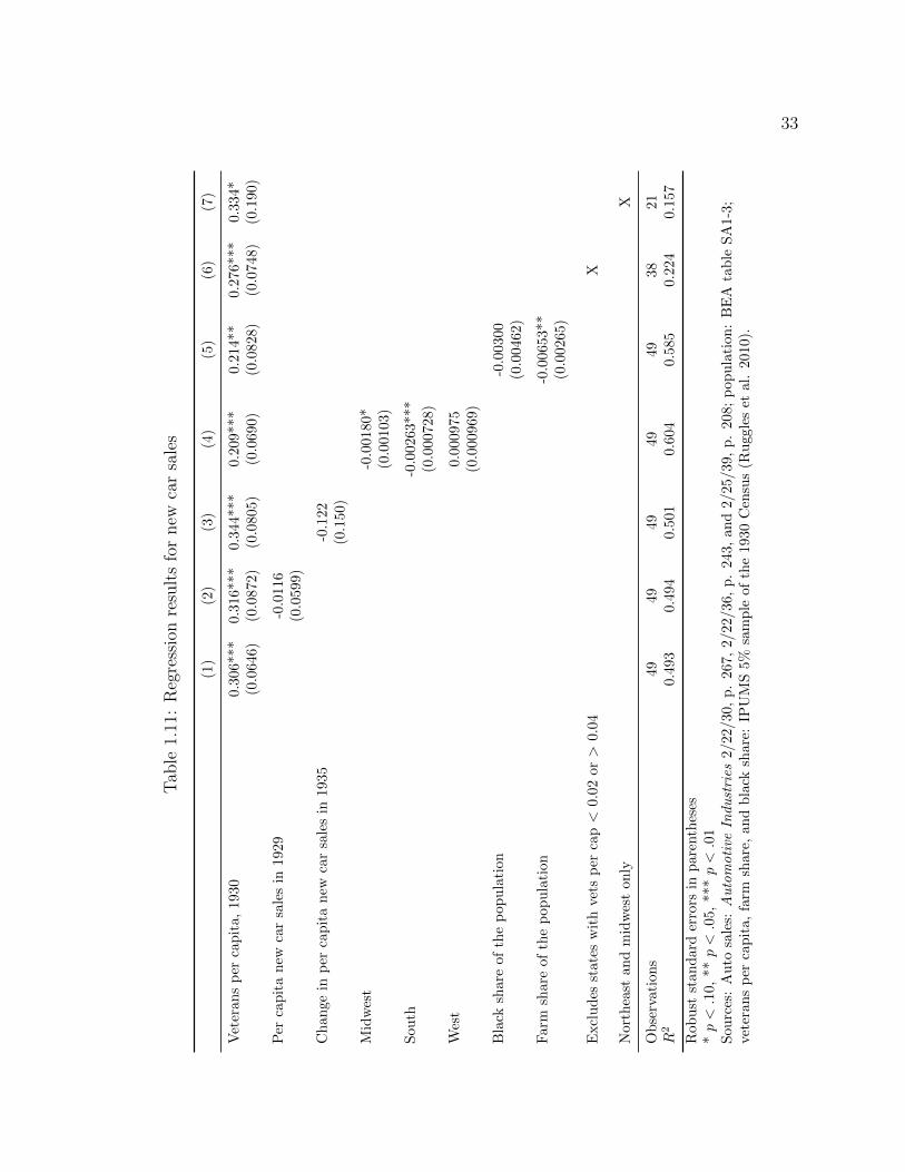
33

Tab

le1.

11:

Reg

ress

ion

resu

lts

for

new

car

sale

s

(1)

(2)

(3)

(4)

(5)

(6)

(7)

Vet

eran

sp

erca

pit

a,19

300.3

06***

0.3

16***

0.3

44***

0.2

09***

0.2

14**

0.2

76***

0.3

34*

(0.0

646)

(0.0

872)

(0.0

805)

(0.0

690)

(0.0

828)

(0.0

748)

(0.1

90)

Per

cap

ita

new

car

sale

sin

1929

-0.0

116

(0.0

599)

Ch

ange

inp

erca

pit

an

ewca

rsa

les

in19

35-0

.122

(0.1

50)

Mid

wes

t-0

.00180*

(0.0

0103)

Sou

th-0

.00263***

(0.0

00728)

Wes

t0.0

00975

(0.0

00969)

Bla

cksh

are

ofth

ep

opu

lati

on-0

.00300

(0.0

0462)

Far

msh

are

ofth

ep

opu

lati

on-0

.00653**

(0.0

0265)

Excl

ud

esst

ates

wit

hve

tsp

erca

p<

0.02

or>

0.0

4X

Nor

thea

stan

dm

idw

est

only

X

Ob

serv

atio

ns

49

49

49

49

49

38

21

R2

0.4

93

0.4

94

0.5

01

0.6

04

0.5

85

0.2

24

0.1

57

Rob

ust

stan

dar

der

rors

inp

aren

thes

es*p<.1

0,**

p<.0

5,**

*p<.0

1S

ourc

es:

Au

tosa

les:

Au

tom

oti

veIn

du

stri

es2/22/30,

p.

267,

2/22/36,

p.

243,

an

d2/25/39,

p.

208;

pop

ula

tion

:B

EA

tab

leS

A1-3

;ve

tera

ns

per

cap

ita,

farm

shar

e,an

db

lack

share

:IP

UM

S5%

sam

ple

of

the

1930

Cen

sus

(Ru

ggle

set

al.

2010).

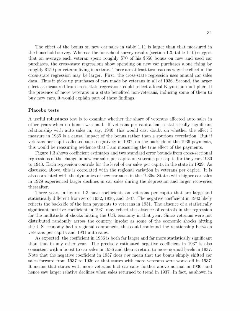
34

The effect of the bonus on new car sales in table 1.11 is larger than that measured inthe household survey. Whereas the household survey results (section 1.3, table 1.10) suggestthat on average each veteran spent roughly $70 of his $550 bonus on new and used carpurchases, the cross-state regressions show spending on new car purchases alone rising byroughly $150 per veteran living in a state. There are at least two reasons why the effect in thecross-state regression may be larger. First, the cross-state regression uses annual car salesdata. Thus it picks up purchases of cars made by veterans in all of 1936. Second, the largereffect as measured from cross-state regressions could reflect a local Keynesian multiplier. Ifthe presence of more veterans in a state benefited non-veterans, inducing some of them tobuy new cars, it would explain part of these findings.

Placebo tests

A useful robustness test is to examine whether the share of veterans affected auto sales inother years when no bonus was paid. If veterans per capita had a statistically significantrelationship with auto sales in, say, 1940, this would cast doubt on whether the effect Imeasure in 1936 is a causal impact of the bonus rather than a spurious correlation. But ifveterans per capita affected sales negatively in 1937, on the backside of the 1936 payments,this would be reassuring evidence that I am measuring the true effect of the payments.

Figure 1.3 shows coefficient estimates and two standard error bounds from cross-sectionalregressions of the change in new car sales per capita on veterans per capita for the years 1930to 1940. Each regression controls for the level of car sales per capita in the state in 1929. Asdiscussed above, this is correlated with the regional variation in veterans per capita. It isalso correlated with the dynamics of new car sales in the 1930s. States with higher car salesin 1929 experienced larger declines in car sales during the depression and larger recoveriesthereafter.

Three years in figures 1.3 have coefficients on veterans per capita that are large andstatistically different from zero: 1932, 1936, and 1937. The negative coefficient in 1932 likelyreflects the backside of the loan payments to veterans in 1931. The absence of a statisticallysignificant positive coefficient in 1931 may reflect the absence of controls in the regressionfor the multitude of shocks hitting the U.S. economy in that year. Since veterans were notdistributed randomly across the country, insofar as some of the economic shocks hittingthe U.S. economy had a regional component, this could confound the relationship betweenveterans per capita and 1931 auto sales.

As expected, the coefficient in 1936 is both far larger and far more statistically significantthan that in any other year. The precisely estimated negative coefficient in 1937 is alsoconsistent with a boost to car sales in 1936 and then a return to more normal levels in 1937.Note that the negative coefficient in 1937 does not mean that the bonus simply shifted carsales forward from 1937 to 1936 or that states with more veterans were worse off in 1937.It means that states with more veterans had car sales further above normal in 1936, andhence saw larger relative declines when sales returned to trend in 1937. In fact, as shown in

35

Figure 1.3: Auto sales and veterans per capita 1930-1940.

-.4-.2

0.2

.4.6

Cha

nge

in c

ar s

ales

per

vet

eran

1930 1931 1932 1933 1934 1935 1936 1937 1938 1939 1940Year

Controls for level of 1929 car salesCoefficient and 2 se bands

Note: Standard errors are the max of conventional and heteroscedasticity robust standarderrors.Sources: Auto sales: Automotive Industries 2/22/30, p. 267, 2/28/31, p. 309, 2/27/32, p.294, 2/25/33, p. 224, 2/24/34, p. 220, 2/22/36, p. 243, 2/25/39, p. 208, 3/1/1940, p. 186,and 3/1/41, p. 214; population: BEA table SA1-3; veterans per capita: IPUMS 5% sampleof the 1930 Census (Ruggles et al. 2010).

table 1.12, the coefficients in figure 1.3 imply that the veterans’ bonus increased the level ofcar sales in 1937 as well as in 1936.

Table 1.12 assumes that the relationship across states between veterans per capita andauto sales hold at the aggregate level. This may be wrong for a variety of reasons.50 Nonethe-less the table provides a useful indication of the rough magnitude of the bonus’s possibleaggregate effects. One initially puzzling result in the table is that absent the bonus carsales would have declined in 1936. This is in fact not unreasonable, since 1935 sales wereboosted by two new model year introductions in the calendar year: one in January and onein November (Cooper and Haltiwanger 1993).51

Housing

The household survey results showed that the largest category of spending from the bonusafter autos was housing. This was housing consumption, e.g. rent and repairs, but it

50See Nakamura and Steinsson 2011 and Mendel 2012.51Readers may also wonder why actual car sales fell so much between 1937 and 1938. In the next chapter,

I argue that this was in part due to the effect of unionization-induced wage and price increases in the autoindustry.

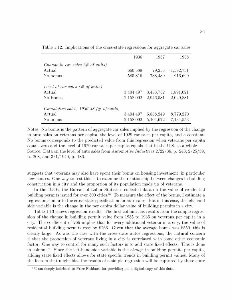
36

Table 1.12: Implications of the cross-state regressions for aggregate car sales

1936 1937 1938

Change in car sales (# of units)Actual 660,589 79,255 -1,592,731No bonus -585,816 788,489 -916,699

Level of car sales (# of units)Actual 3,404,497 3,483,752 1,891,021No Bonus 2,158,092 2,946,581 2,029,881

Cumulative sales, 1936-38 (# of units)Actual 3,404,497 6,888,249 8,779,270No bonus 2,158,092 5,104,672 7,134,553

Notes: No bonus is the pattern of aggregate car sales implied by the regression of the changein auto sales on veterans per capita, the level of 1929 car sales per capita, and a constant.No bonus corresponds to the predicted value from this regression when veterans per capitaequals zero and the level of 1929 car sales per capita equals that in the U.S. as a whole.Source: Data on the level of auto sales from Automotive Industries 2/22/36, p. 243, 2/25/39,p. 208, and 3/1/1940, p. 186.

suggests that veterans may also have spent their bonus on housing investment, in particularnew houses. One way to test this is to examine the relationship between changes in buildingconstruction in a city and the proportion of its population made up of veterans.

In the 1930s, the Bureau of Labor Statistics collected data on the value of residentialbuilding permits issued for over 300 cities.52 To measure the effect of the bonus, I estimate aregression similar to the cross-state specification for auto sales. But in this case, the left-handside variable is the change in the per capita dollar value of building permits in a city.

Table 1.13 shows regression results. The first column has results from the simple regres-sion of the change in building permit value from 1935 to 1936 on veterans per capita in acity. The coefficient of 266 implies that for every additional veteran in a city, the value ofresidential building permits rose by $266. Given that the average bonus was $550, this isclearly large. As was the case with the cross-state autos regressions, the natural concernis that the proportion of veterans living in a city is correlated with some other economicfactor. One way to control for many such factors is to add state fixed effects. This is donein column 2. Since the left-hand-side variable is the change in building permits per capita,adding state fixed effects allows for state specific trends in building permit values. Many ofthe factors that might bias the results of a simple regression will be captured by these state

52I am deeply indebted to Price Fishback for providing me a digital copy of this data.

37

Table 1.13: Regression results for residential building permits

(1) (2) (3) (4) (5)

Veterans per capita, 1930 265.9*** 209.6*** 127.9*** 119.7*** 204.4***(82.25) (76.98) (47.20) (37.15) (61.22)

∆ per capita bldg. permits 1935 0.823***(0.107)

Black share of the population 4.884*(2.776)

State fixed effects X X X

Outliers excluded X X X

Cities with pop. > 50,000 only X

Observations 302 302 282 282 172R2 0.086 0.275 0.362 0.422 0.486

Standard errors clustered at the state level in parentheses

* p < .10, ** p < .05, *** p < .01

Sources: The building permit data is from Price Fishback who collected it from various editions of the

Bureau of Labor Statistics Monthly Labor Review and from Bureau of Labor Statistics (1938, 1940).

Veterans per capita and black share come from the IPUMS 5% sample of the 1930 Census

(Ruggles et al. 2010).

specific trends: for instance, if veterans per capita is correlated with agricultural productionof a specific crop or climate shocks.

In fact, the coefficient is little affected by the addition of the state fixed effects. Moreimportant is whether one drops outliers. In column 3, I drop the 10 cities with the smallestand largest per capita building permit changes. This shrinks the coefficient, but it remainshighly economically and statistically significant. Column 4 controls for the lagged changein building permit values and the share of the population that was black. This resultsin a coefficient very similar to that with state fixed effects. A different way to test therobustness of the results is to limit the sample. In column 5, the sample is restricted to citieswith a population greater than 50,000 (in 1930). This significantly increases the size of thecoefficient.

A final check on these results is placebo tests. Figure 1.4 shows the coefficient and twostandard error bands for the three years for which I have data - 1935, 1936, and 1937. Theonly year with a large and statistically significant effect is 1936. Interestingly, unlike forauto sales, the coefficient in 1937 is not negative. This suggests that positive effects of thebonus on residential construction may have persisted beyond 1936. Given the lags involvedin planning construction and obtaining a building permit, this is unsurprising.

Taken together, the results in table 1.13 and figure 1.4 imply that the bonus had large and

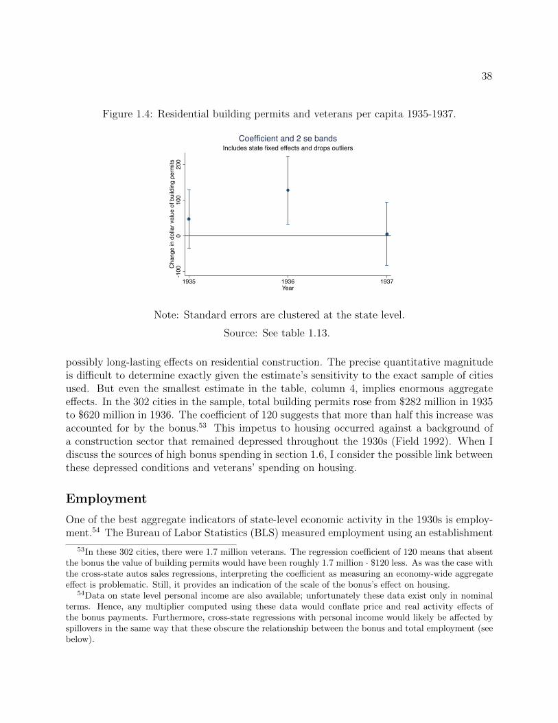
38

Figure 1.4: Residential building permits and veterans per capita 1935-1937.

-100

010

020

0C

hang

e in

dol

lar v

alue

of b

uild

ing

perm

its

1935 1936 1937Year

Includes state fixed effects and drops outliersCoefficient and 2 se bands

Note: Standard errors are clustered at the state level.

Source: See table 1.13.

possibly long-lasting effects on residential construction. The precise quantitative magnitudeis difficult to determine exactly given the estimate’s sensitivity to the exact sample of citiesused. But even the smallest estimate in the table, column 4, implies enormous aggregateeffects. In the 302 cities in the sample, total building permits rose from $282 million in 1935to $620 million in 1936. The coefficient of 120 suggests that more than half this increase wasaccounted for by the bonus.53 This impetus to housing occurred against a background ofa construction sector that remained depressed throughout the 1930s (Field 1992). When Idiscuss the sources of high bonus spending in section 1.6, I consider the possible link betweenthese depressed conditions and veterans’ spending on housing.

Employment

One of the best aggregate indicators of state-level economic activity in the 1930s is employ-ment.54 The Bureau of Labor Statistics (BLS) measured employment using an establishment

53In these 302 cities, there were 1.7 million veterans. The regression coefficient of 120 means that absentthe bonus the value of building permits would have been roughly 1.7 million · $120 less. As was the case withthe cross-state autos sales regressions, interpreting the coefficient as measuring an economy-wide aggregateeffect is problematic. Still, it provides an indication of the scale of the bonus’s effect on housing.

54Data on state level personal income are also available; unfortunately these data exist only in nominalterms. Hence, any multiplier computed using these data would conflate price and real activity effects ofthe bonus payments. Furthermore, cross-state regressions with personal income would likely be affected byspillovers in the same way that these obscure the relationship between the bonus and total employment (seebelow).

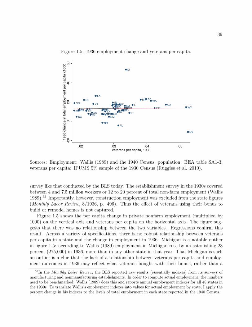
39

Figure 1.5: 1936 employment change and veterans per capita.

AL

AZ

ARCA

COCT

DE

FL

GAID

ILIN

IA

KS

KY

LA

ME MD MA

MI

MNMS

MO

MT

NE

NV

NH

NJ

NM

NY

NC

ND

OH

OK

ORPA RI

SC

SDTN TXUT

VT

VA

WA

WV

WIWY

-20

020

4060

1936

cha

nge

in to

tal e

mpl

oym

ent p

er c

apita

x10

00

.02 .03 .04 .05Veterans per capita, 1930

Sources: Employment: Wallis (1989) and the 1940 Census; population: BEA table SA1-3;veterans per capita: IPUMS 5% sample of the 1930 Census (Ruggles et al. 2010).

survey like that conducted by the BLS today. The establishment survey in the 1930s coveredbetween 4 and 7.5 million workers or 12 to 20 percent of total non-farm employment (Wallis1989).55 Importantly, however, construction employment was excluded from the state figures(Monthly Labor Review, 8/1936, p. 496). Thus the effect of veterans using their bonus tobuild or remodel homes is not captured.

Figure 1.5 shows the per capita change in private nonfarm employment (multiplied by1000) on the vertical axis and veterans per capita on the horizontal axis. The figure sug-gests that there was no relationship between the two variables. Regressions confirm thisresult. Across a variety of specifications, there is no robust relationship between veteransper capita in a state and the change in employment in 1936. Michigan is a notable outlierin figure 1.5: according to Wallis (1989) employment in Michigan rose by an astonishing 23percent (275,000) in 1936, more than in any other state in that year. That Michigan is suchan outlier is a clue that the lack of a relationship between veterans per capita and employ-ment outcomes in 1936 may reflect what veterans bought with their bonus, rather than a

55In the Monthly Labor Review, the BLS reported raw results (essentially indexes) from its surveys ofmanufacturing and nonmanufacturing establishments. In order to compute actual employment, the numbersneed to be benchmarked. Wallis (1989) does this and reports annual employment indexes for all 48 states inthe 1930s. To translate Wallis’s employment indexes into values for actual employment by state, I apply thepercent change in his indexes to the levels of total employment in each state reported in the 1940 Census.

40

small multiplier. Suppose in the extreme case that every veteran bought a new car with hisbonus check and nothing else. In this case, the aggregate effect of the bonus would obviouslyhave been large: 3.2 million more new cars would have been sold. And this effect wouldshow up in a cross-state regression of auto sales on veterans’ share. But the employmenteffects would be concentrated in Michigan and other heavily industrialized states. Hencethere might be no relationship between state level employment changes in 1936 and veteransper capita. Of course, veterans did not only buy cars. But the results of section 1.3 suggestthat they primarily bought tradable goods (and housing).

1.5 Direct survey and narrative evidence

The American Legion Survey

In the recent literature on consumption responses to transfers there are two dominant ap-proaches. One is to use Consumer Expenditure (CE) Survey data to directly measure spend-ing from a transfer payment. Influential examples are Johnson, Parker, and Souleles (2006)on the effect of the 2001 Bush tax cuts, and Parker, Souleles, Johnson and McClelland(2011) on the effect of the 2008 stimulus payments. An alternative approach is to ask peoplewhether they plan to spend a transfer payment. Shapiro and Slemrod (2003, 2009) do thisby adding a question to the Michigan Survey of Consumers.

A rough equivalent to Shapiro and Slemrod’s exercise can be replicated for the 1936Veterans’ Bonus. In January 1936, the American Legion surveyed 42,500 of its membersabout what they planned to do with their bonus. At the time, the American Legion was theleading World War I veterans’ group, and it played a large role in lobbying for the bonus’spassage (Daniels 1971). The survey is shown in figure 1.6. While the actual survey responsesno longer exist, the American Legion library has a copy of unpublished tabulations preparedby an Indianapolis accounting firm on behalf of the American Legion. Table 1.14 showsthese tabulations.

Two caveats are needed before discussing the results. First, the survey was done beforethe exact legislative details of the bonus were known, and in particular before it was knownwhether veterans would be allowed to leave their bonus with the government and earn 3percent interest on it. Thus the survey estimates may somewhat understate total savingfrom the bonus. Second, the American Legion population was not identical to that of allveterans. It is possible that what was true about spending for Legion members was nottrue for veterans as a whole. Despite these caveats, the tabulations of the survey do provideinformation on the spending plans of a large population of veterans.

The results show that veterans planned to use 37 percent of the bonus to save or paydown debt. Interestingly, nearly all of this is accounted for by debt repayment: perhapsunsurprisingly, in 1936 few appeared eager to invest their bonus in financial markets. Ofthe remaining 63 percent of the bonus, veterans said they planned to spend 25 percent onbusiness and residential investment and the remainder on consumption: the implied MPC is

41

Figure 1.6: American Legion survey form

42

Table 1.14: American Legion survey tabulations

Item Amount per veteran Percent of bonus

Repair present house $ 37.90 6.71%Paint house $ 9.72 1.72%Housing consumption total $ 47.62 8.43%

Furniture $ 17.37 3.07%Rugs and carpets $ 2.83 0.50%Other house furnishings $ 12.93 2.29%Electric or gas refrigerator $ 6.04 1.07%Oil or gas furnace $ 2.57 0.45%Radio $ 2.49 0.44%Other durable gds total $ 44.22 7.82%

Suit or overcoats $ 9.84 1.74%Shirts $ 0.87 0.15%Shoes $ 0.99 0.18%Hats $ 0.48 0.08%Other men’s furnishings $ 2.48 0.44%Clothing for children $ 12.01 2.13%Clothing for wife $ 13.10 2.32%Clothing total $ 39.76 7.04%

Passenger automobiles $ 30.86 5.46%Trucks $ 4.02 0.71%Automobile tires $ 1.52 0.27%Automobile batteries $ 0.15 0.03%Autos total $ 36.55 6.47%

Purchase farm $ 18.97 3.36%Farm implements $ 12.46 2.20%Invest in own business $ 37.90 6.71%Build new house $ 26.28 4.65%Purchase home $ 36.80 6.51%Purchase lot for homesite $ 9.03 1.60%Investment total $ 141.43 25.03%

Purchase insurance $ 19.11 3.38%Education $ 5.08 0.90%Miscellaneous $ 22.72 4.02%Other total $ 46.91 8.30%

Pay old bills and debts $ 177.26 31.36%Savings accounts $ 25.26 4.47%Purchase stocks or bonds $ 6.15 1.09%Savings total $ 208.68 36.92%

43

0.38. Of course, in determining the short-run aggregate effects of the bonus what matters isthe total amount that was spent, not whether it was spent on investment or consumption.

For comparison, using a question on household spending plans added to the MichiganSurvey of Consumers, Shapiro and Slemrod (2003, 2009) find an MPC of roughly 1/3 forboth the 2001 and 2008 tax cuts. By contrast, Parker et al. (2006, 2011) find an actualMPC using the CE survey of 2/3 in 2001 and between 0.5 and 0.9 in 2008. It appears that atleast part of the difference between these methodologies comes from the measurement of thelagged spending response.56 Johnson, Parker and Souleles (2006) find a MPC in the quarterthe 2001 tax rebate was received similar to that measured in Shapiro and Slemrod (2003).But Johnson, Parker and Souleles also find a substantial spending response in the followingquarter. A possible explanation is that many households told the Michigan survey that theyplanned to use the rebate to pay down debt and that these households initially did exactlythis. But over the months following the rebate, households may have responded to lowerdebt by spending more, a response they may not have considered when predicting how therebate would affect their spending. Agarwal, Liu, and Souleles (2006) analyze credit cardspending and debt in 2001 and find evidence for this behavior.

Thus it is possible that the American Legion survey accurately predicted the immediateresponse but not continued spending. In any case, the modern evidence suggests that thefinding of an MPC in the Legion survey of 0.38 is fully consistent with the MPC of 0.6 to0.75 found using the 1935-36 consumption survey. Indeed, since the American Legion resultssuggest substantial spending on residential and business investment as well as consumption,they imply that the total marginal propensity to spend was somewhat above the marginalpropensity to consume. The substantial spending on new home purchases and constructionindicated by the American Legion survey fits with the cross-city building permit evidence.Together these two sources provide strong evidence that veterans spent a significant portionof their bonus on housing investment.

Direct comparison of survey results for consumption categories with results from thehousehold survey are complicated by differences in category definitions. Still, it is possibleto make some comparisons. Naturally, since the overall MPC is lower, in most categories theAmerican Legion survey also suggests lower spending. For example, the household surveysuggests that the average veteran spent $83 of his bonus on housing consumption while theAmerican Legion survey suggests they planned to spend $48. (Recall that the average bonusreceived by a veteran was $547.) The difference for auto purchases is larger: $71 versus $35,possibly reflecting the fact that demand for cars in the 1930s was generally low in winter,when the American Legion survey was given, but high in summer, when the bonus paymentsarrived. Buying a car was more attractive when roads were not mired in mud.57

56See Shapiro and Slemrod (2009), p. 378 for a discussion of this issue.57Busse, Pope, Pope, and Silva-Risso (2012) provide modern evidence for this kind of effect in the car

market. They find that SUV sales are unusually high when the weather is cold or snowy. They argue thatthis reflects ‘projection bias’ - people assuming that their future utility from a car purchase will be similar tothe current utility. In the 1930s, when SUVs did not exist and unpaved roads could be literally impassablein winter, it is likely that veterans’ surveyed in January were unable to fully imagine how much they would

44

Narrative Evidence

A useful check on the quantitative evidence of previous sections comes from newspaperreports at the time: given my results, it would be troubling if newspapers did not reporthigh spending by veterans. In fact, they reported a spending boom.

For example, the Los Angeles Times wrote on June 19, 1936, four days after the bonuswas distributed (p. A1):

All signs yesterday pointed to a real spending spree by veterans. . . . Downtowndepartment stores reported yesterday’s sales were more than 30 percent above aweek ago.

The Wall Street Journal reported a couple weeks later, on July 3 (p. 1):

Unusual gains in retail sales of new passenger cars the latter part of last monthlifted the June retail sales totals of the largest automobile units to new peaks forthe year. . . . Such a development was not expected, the belief of automobilepeople being that June sales would not be able to maintain the fast pace ofApril and May, usual months for peak in new car sales. No doubt the bonushad something to do with pushing sales into new high ground, but generallystrong business throughout most of the country played an equal part in providingsupport.

Of course, the “generally strong business” referred to by the Wall Street Journal may itselfreflect the effect of the bonus.

Dun and Bradstreet Monthly Review noted the effects of the veterans’ bonus in its July1936 report on business conditions around the country during June (pp. 45-47). Some citiesreported little effect, at least in the first two weeks of bonus distribution. In others, however,effects were evidently visible and large. For example, the report from the Minneapolis regionsaid (p. 46):

The depressing results of severe drought conditions which have developed inNorth Dakota, Montana, and portions of South Dakota have been more thanoffset by the exhilarating effect of the spending of bonus money.

The negative effects of drought and heatwave come up frequently in contemporary narrativereports. In 1936, drought afflicted much of the country and was particularly severe in theDakotas and Kansas.58 And July 1936 was extraordinarily hot in much of the midwest.Temperatures reached 110 degrees in Iowa and Wisconsin.59 As noted in the above quote,this makes it all the more remarkable that large effects of the bonus are detectable both inthe data and in narrative evidence.

want to buy a car come summer.58See http://www.ncdc.noaa.gov/paleo/pdsiyear.html.59See http://www.crh.noaa.gov/arx/events/heatwave36.php.

45

Figure 1.7: From the Chicago Tribune, 6/14/36, p. 1

46

The front page of the Chicago Tribune on June 14, 1936 - the day before the bonus wasdistributed - printed a cartoon showing the businesses hoping for a share of the bonus money(figure 1.7). The cartoon suggests that contemporaries expected the money to be used topurchase a wide variety of consumer goods. Note in particular the prominent position of theauto dealer (and Ye Olde Tappe Room). The savings bank is far in the rear.

1.6 Why was the MPC so high?

A variety of evidence suggests that veterans quickly spent the majority of their bonus. Thisis in some ways puzzling. The conventional wisdom is that when transfer payments are verylarge, as the bonus was, the MPC should be relatively small. Empirical evidence for thisview comes from Hsieh (2003) who looks at the consumption response to annual paymentsfrom the Alaska Permanent Fund. He finds a MPC of zero. By contrast, Souleles (1999)looks at the consumption response to annual income tax refunds and finds a MPC of between0.35 and 0.65. Hsieh (2003) speculates that he finds a lower response because payments fromthe Alaska Permanent Fund differ in important ways from income tax funds. In particular,they are larger and more predictable. In both respects, the bonus was probably more similarto the Alaska Fund Payments than to income tax refunds. Certainly the bonus paymentswere larger. And although they were not regular in the sense that annual payments fromthe Alaska Fund are, they varied less across individuals than income tax refunds and wererelatively straightforward to calculate. A veteran simply had to take the value of his adjustedservice certificate and subtract the amount of any loans taken.

Behavioral economists have also argued that the MPC should decline with the size of thepayment. Whereas small payments may be put in mental ‘income’ account from which theMPC is large, large payments, such as the veterans’ bonus, may be put in a mental ‘asset’account from which the MPC is small. Shefrin and Thaler (1988, p. 635) put it this way:“The larger is a windfall, the more wealth-like it becomes, and the more likely it will beincluded in the less tempting Assets account.”

Why then did World War I veterans spend so much of their bonus? Although an ex-planation is necessarily speculative, I believe that three features of the 1936 economy werecritical: (1) people faced substantial liquidity constraints; (2) future income was expectedto be higher, and (3) there was substantial pent-up demand for durables, in particular carsand housing.

Liquidity constraints

The interwar period saw an explosion of consumer debt; consumer non mortgage debt as apercent of income rose from 4.6 percent in 1919 to 11.4 percent in 1939 (Olney 1999, tableI). However, all consumer debt was short-term (less than three years) and often came withonerous terms (Olney 1991). A typical car loan required a 33 percent downpayment if anew car, and a 40 percent downpayment if a used car (Olney 1991, p. 113). The maximum

47

maturity length of a car loan was 18 months, with a typical interest rate, including all financecosts, of 20 to 40 percent (Olney 1991, p. 115). Thus the typical veteran, while able to takeout a loan to finance a car or other large durable good purchase, in practice may still havebeen constrained by the large downpayment requirements. And of course harsh loan termsprovided an incentive to buy goods with cash rather than on credit, even if this meant anuneven time path of consumption.

Veterans may have found borrowing easier as the date of bonus disbursement approached:some narrative evidence reports loans being targeted to veterans in advance of the bonuspayment. However, the combination of the household consumption survey results that areidentified off the timing of the bonus disbursement and narrative evidence suggests thatliquidity constraints remained binding for many if not most veterans throughout spring1936. The Magazine of Wall Street wrote in May 1936 “[A] great many veterans lack creditstanding and have not been able to spend in anticipation of the windfall” (5/9/36, p. 77).60

Expectations of higher future income

Liquidity constraints alone cannot generate a high MPC. There must be a reason why theconstraint binds, why the consumer would like to borrow but cannot. If consumers wishto save, liquidity constraints do not increase the MPC. In fact, the possibility of liquidityconstraints binding in the future increases the incentive to save today. The most obviousreason why veterans may have wished to borrow is that they expected their income in thefuture to be higher. A consumption smoothing motive would then lead them to want toborrow against their future income. In this situation, veterans might reasonably have spentmuch or even all their bonus in the months after receipt.

Veterans may have expected higher future income because most probably saw their in-comes rise rapidly in the three years prior to the bonus. Real per capita personal income rose19 percent from 1933 to 1935.61 And while it is not possible to directly measure veterans’expectations, economic forecasters in early summer 1936 expected good times to continue.A representative quote comes from the Magazine of Wall Street 6/20/36, p. 296 under theheadline “Signs of Business Progress:”

60The full quote is as follows:

Beyond question [the bonus] will prove an important stimulus to total business activity, al-though, of course, two major uncertainties are involved in attempting to forecast the resultswith any degree of accuracy. For one thing, not all of the approximately $2,000,000 of bonusmoney will be spent. For another thing, it is quite certain that some part of it has alreadybeen spent in anticipatory resort to credit and, in less measure, in withdrawals from presentsavings. On the other hand a great many veterans lack credit standing and have not been ableto spend in anticipation of the windfall.

On the subject of car purchases in advance of the bonus payment the industry trade publication AutomotiveIndustries reported (6/20/36, p. 857): “While some advance business has been done on credit in anticipationof the bonus, the amount is said to be small.”

61NIPA table 2.1.

48

[T]here is every indication that the usual summer lag is to be less than normal.Automobile assemblies have held up remarkably well; the steel industry is op-erating at a high rate of capacity; while retail trade will be stimulated at anunusual time by the payment of the solders’ bonus. A wafted straw indicates thedirection of the wind and below will be found a number of straws showing thewind is still a fair one.

The Magazine of Wall Street did not venture a guess about economic conditions beyond thesummer, but the tone suggests optimism.

A concrete measure of expectations of future income is the behavior of the stock market.62

In the four years from its low in June 1932, the market rose 208 percent. In just the yearprior to the bonus disbursement, from June 1935 to June 1936, the market rose 45 percent.63

Thus market participants, at least, were optimistic. And the bonus disbursement may haveincreased their optimism: between June and July 1936, the market rose 6 percent.

Demand for autos and housing

In theory, expectations of higher future income combined with liquidity constraints couldgenerate a MPC as high as 1. In practice it seems unlikely that this alone could explain thehigh MPC that I observe. After all, even if many veterans expected higher future income,there must also have been some who remained pessimistic and uncertain after the veryrecent declines in income during the Depression itself. It seems likely that a key additionalcontributor to high spending from the bonus was pent-up demand for autos and housing.

Of course, from the point of view of a household, spending on durables and housingis a form of saving. Thus there is little conflict between standard neoclassical models ofconsumption and a large marginal propensity to spend on durables. But although from thehousehold’s perspective purchasing a car and depositing money in the bank are similar, forthe aggregate economy, the implications are entirely different: in the former case, a transferpayment succeeds at increasing spending, in the latter it does not.

What will determine whether households choose to save a transfer or purchase a car?Berger and Vavra (2012) consider a business cycle model in which consumers face fixedcosts of adjustment when buying durables.64 This leads to Ss policy functions. The keydeterminant of the marginal propensity to spend on cars (or other durables) is the gapbetween consumers’ current stock of durables and their target stock. When this gap is large,

62Not only are stock prices an indicator of market participants’ expectations, the behavior of the stockmarket was a salient indicator that may have been viewed by the broader public as a predictor of futureincome. This could have been the case despite the fact that only a small percent of American householdsactually owned stocks (Romer 1990).

63Stock price data are for the S&P composite index and are from Robert Shiller. See http://www.econ.

yale.edu/~shiller/data.htm.64For other models of auto purchases, see Adda and Cooper (2000) and House and Leahy (2004). While

neither of these papers studies the implications of their models for the MPC, their implications would likelybe similar to those in Berger and Vavra (2012).

49

many households will be close to their trigger point. In this case, a transfer payment - evena relatively small one - may lead many households to buy a car. This was likely the case in1936. Despite the Depression, the period from 1929 to 1936 saw a rapid expansion of thepaved road network (Field 2011), and a rapid decline in the quality-adjusted price of autos.Real, quality-adjusted, car prices fell 17 percent from 1928 to 1936 (Raff and Trajtenberg1996, table 2.6). Yet, the stock of passenger cars in use was lower at the end of 1935 than itwas at the end of 1929 (Roos and Van Szeliski 1939, p. 50). Many households were almostsurely anxious to buy a new car as soon as their incomes permitted. The existence of manyhouseholds close to such a threshold can explain why the bonus had such large effects oncar purchases. Indeed, insofar as some veterans used the bonus to purchase a car that costmore than the bonus (either by borrowing or drawing down savings), it is even possible thatfor some the MPC exceeded 1.

For housing, a similar story likely applied. To a remarkable degree, residential investmentdid not recover in the 1930s. Total residential investment over the three years from 1933 to1935 was less than that in the single year 1929.65 Field (1992) argues that the persistent lowlevel of residential construction was due in large part to the physical and legal barriers leftby haphazard land development in the 1920s. The effect was to make the stock of residentialfixed assets, like the stock of automobiles, lower in 1935 than it had been in 1929 despite 4.5percent population growth.66 Thus just as many veterans were likely anxious to purchase anew car, many were also likely eager to buy a new house or move to a nicer apartment.

1.7 Aggregate effects of the bonus

A back-of-the-envelope calculation

The aggregate multiplier associated with the bonus was a function of two things: (1) howmuch of each dollar of bonus payments was spent, and (2) the spending multiplier. Thischapter provides evidence on the former. Many recent theoretical and empirical papersprovide estimates of the later. A robust conclusion of this literature is that multipliers arelikely to be significantly higher when interest rates are at the zero lower bound, as theywere in 1936. Many papers find multipliers in the range of 1.5 to 2 (or possibly higher) inthese conditions.67 And a surprising number of estimates from both theory and empirics

65NIPA table 1.1.3.66BEA fixed asset table 5.2 and http://www.census.gov/popest/data/national/totals/pre-1980/

tables/popclockest.txt67For example, Gordon and Krenn (2010) find that the multiplier for government spending in 1940 was 1.8,

and Alumnia et al. (2010) estimate that the defense spending multiplier in the 1930s was 2.5. New KeynesianDSGE models suggest that these estimates are reasonable. See, for instance, Hall (2009), Woodford (2011)and Christiano, Eichenbaum, and Rebelo (2011). Of course, the exact value of the spending multiplier iscontroversial. While much of the literature suggests that 1.5 to 2 is a reasonable range at the zero lowerbound, the multipliers measured in the empirical literature inevitably come with confidence intervals thatencompass much smaller and larger values. And multipliers derived from New Keynesian models are sensitive

50

are clustered in the narrow range of 1.6 to 1.8. For instance, Hall (2009) finds a spendingmultiplier of 1.7 in a simple New Keynesian model at the zero lower bound, and Gordonand Krenn (2008) empirically estimate that the spending multiplier in the U.S. in 1940 was1.8. The evidence from the household consumption survey suggests that the MPC fromthe bonus was 0.6 to 0.75. And the American Legion survey and cross-city building permitregressions suggest that veterans spent significant amounts of their bonus on investment aswell as consumption. Thus it is reasonable to think that the total marginal propensity tospend on consumption and investment is likely to have been near if not above the high endof this range. In the following, I assume that it was 0.7.

The implied multiplier associated with the bonus is then 0.7·Sm, where Sm is the spendingmultiplier. One can compute the aggregate effect of the bonus on GDP growth as thismultiplier times a measure of the bonus in real terms divided by real 1935 GDP:

(Y36

Y35

− 1)︸ ︷︷ ︸Actual ’36 growth

− (Y36 −B · P37

P36· 0.7 · Sm

Y35

− 1)︸ ︷︷ ︸Counterfactual ’36 growth

=B · P37

P36· 0.7 · Sm

Y35︸ ︷︷ ︸Bonus’s effect on growth

, (1.8)

where B is the nominal bonus amount and Pt is the price index in year t. I measure pricesusing the GDP price index;68 real output is measured in chained 1937 dollars.69 Table 1.15shows the result of this calculation for several possible values of the spending multiplier.Regardless of one’s prior for the spending multiplier, the high MPC that I find suggestsa significant effect of the bonus. Even if the spending multiplier were only 0.5, the bonusadded nearly a percentage point to 1936 GDP. For the most likely values of the multiplier,around 1.7, this calculation suggests an effect on GDP growth of 2.5 to 3 percentage points.An Okun’s law coefficient of 2 would then imply a decline in the unemployment rate due tothe bonus of 1.3 to 1.5 percentage points.70

to assumptions about the form of the utility function, the degree of price stickiness and the persistance ofthe shock. For an argument that the multiplier may be somewhat smaller, see Ramey (2011).

There are two reasons to think that applying modern estimates of the multiplier to conditions in 1936may be conservative. First, the high MPC among veterans that I measure suggests that the MPC in thepopulation as a whole may have been high. This implies that the spending multiplier in the mid 1930s mayhave been larger than is usually thought. In standard New Keynesian DSGE models factors likely to raisethe MPC, such as a large proportion of hand-to-mouth consumers, also tend to raise the multiplier. Second,modern empirical estimates of the multiplier reflect the fact that the U.S. economy is open, and thus asignificant amount of spending leaks abroad. By contrast, in 1936 the U.S. was much closer to being a closedeconomy: imports were 4 percent of GDP then versus 18 percent today (NIPA table 1.1.5). Furthermore, thelevel of real imports was unchanged from 1935 to 1936, despite the large increase in output and consumption(NIPA table 1.1.6). This strongly suggests that very little of the bonus was spent on foreign produced goods.Other things being equal, this ought to have increased the multiplier associated with the bonus.

68NIPA table 1.1.4.69NIPA table 1.1.6a.70Readers may wonder whether Okun’s law provides a good approximation in the 1930s. In fact, the

evidence suggests that Okun’s law has been remarkably constant over time. For instance, Romer (1986)finds an Okun’s law coefficient near 2 for the period 1893 to 1927.

51

Table 1.15: Effect of the bonus on 1936 GDP growth

Spending multiplier Effect on ’36 growth (percentage points)

0.5 0.81.0 1.71.5 2.51.7 2.82.0 3.3

Source: See text.

The aggregate time series

Since the 1936 veterans’ bonus was a single event, it is not possible to use aggregate timeseries to establish causal effects of the bonus. Still, the time series are suggestive. One wayto see if the above calculation is plausible is to compare the path of GDP, consumption,and investment in 1936 to that in other years of the recovery. This is done in table 1.16.The rapid increase in GDP in 1936 is obvious: whereas GDP grew 10.9 percent in 1934,and 8.9 percent in 1935, it grew over 13 percent in 1936. Most of the increase in growthwas driven by a dramatic increase in consumption. Consumption growth increased by fourpercentage points from 1935 to 1936. This aggregate increase in consumption was reflectedin subcategories: June to June increases in department store sales, variety store sales, andauto sales were all larger in 1936 than they had been in 1934 or 1935.71

Table 1.16: Real output, consumption, and investment (billions of 2005 dollars)

GDP Consumption Investment

1933 715.8 600.8 18.91934 793.7 643.7 34.11935 864.2 683 63.11936 977 752.5 80.91937 1027.1 780.4 101.1

Source: NIPA table 1.1.6.

All this is not easily explained by factors other than the bonus. Monetary factors were ifanything contractionary in 1936. Broad money supply growth slowed from 14 percent in 1935

71See Survey of Current Business, August 1936, p. 6. Telser (2003) provides a more detailed analysis ofmonthly time series and the evidence they provide in favor of large effects from the bonus.

52

to 11 percent in 1936.72 And in August 1936, the Federal Reserve raised reserve requirements.While the reserve requirement increase probably had little direct effect on the economy,73

it signaled a monetary regime shift that could have lowered inflation expectations and thusraised real interest rates (Eggertsson and Pugsley 2006). No doubt it would be possible toconstruct a story in which because of long lags, money growth in past years explains theextraordinary growth of output in 1936.74 But a more plausible story is that the bonus wasthe key factor raising 1936 growth well above its 1934 or 1935 levels. Compared to monetarypolicy, the bonus can also more easily account for why so much of 1936 growth was drivenby consumption.

The Bonus and the 1937-38 Recession

The boom year of 1936 was followed by slower growth in 1937 and actual contraction in1938. The backside of the bonus can explain why growth slowed from 1936 to 1937: if largeamounts were spent from the bonus in 1936, then a return of spending to trend in 1937would be reflected in slower growth. This argument does not imply that the bonus loweredthe level of output or welfare in 1937, only that it reduced growth in that year. I providedevidence for exactly this scenario from the cross-state auto sales regressions. These suggestedthat the bonus significantly lowered autos sales growth in 1937, despite slightly increasingthe level of sales in that year.

As pointed out by Romer (1992), Irwin (2011), and the next chapter, it is less clear thatfiscal policy, and the veterans’ bonus in particular, can account for the 1937-1938 recession.One problem is the magnitude of the bonus. The bonus, a 2 percent of GDP payment,cannot account for the change from 13.1 percent GDP growth in 1936 to -3.4 percent GDPgrowth in 1938.75 But despite the lack of an overwhelming direct effect, there are also atleast two channels through which the bonus conceivably contributed indirectly to the 1937-38recession.

First, Irwin (2011) argues that the 1937-38 recession was primarily caused by the Trea-sury’s decision to sterilize gold inflows beginning in December 1936. This decision waspartly motivated by increases in wholesale prices in the second half of 1936 (Irwin 2011).And these price increases were undoubtedly boosted by the veterans’ bonus. Indeed, inso-far as the bonus increased inflation and thus lowered real interest rates, this is one of themechanisms through which it facilitated economic recovery. But the Treasury cut-off thisvirtuous cycle when it began sterilization in December.

72The source is NBER macrohistory series m14144a, which is computed from underlying data in Friedmanand Schwartz (1970), Monetary Statistics of the United States.

73See Calomiris, Mason, and Wheelock 2011 and Irwin 2011.74If one estimates a simple regression of output growth on lags of output growth and the money supply

with annual data from 1919-1940, one obtains a good fit for all years after 1933 except 1936 and 1938. In1936, growth is 4.5 percentage points above the prediction from this forecast regression. At least in thisreduced form setting, the lagged effect of money supply growth appears not to be a plausible explanationfor rapid 1936 GDP growth.

75NIPA table 1.1.1.

53

Second, in the next chapter I argue that monetary factors alone cannot explain the fullextent of the 1937-38 recession. In addition to the backside of the veterans’ bonus, otherfiscal factors, in particular the beginning of social security tax collection in January 1937,contributed to slower growth. A separate contractionary factor was a supply shock to theauto industry. Chapter two argues that unionization-induced auto price increases took over apercentage point off output growth in 1936. More generally, economy-wide unionization mayhave had a negative effect on growth in 1937 and 1938 (Cole and Ohanian 2001). But again,the veterans’ bonus may not escape all blame. The decision of auto and other manufacturersto accede to union demands was plausibly in part a result of the high level of sales in 1936induced by the bonus. Had sales been lower, manufacturers might have felt more pressureto deny workers wage increases.

1.8 Conclusion

This chapter studies the effects of a 1936 payment to World War I veterans totaling 2 percentof GDP. It uses cross-sectional data to identify the effects of the so-called veterans’ bonus onconsumption. I find that within six months of receipt, veterans spent the majority of theirbonus. The primary evidence comes from the 1935-36 Study of Consumer Purchases. Usinga differences-in-differences estimation strategy, I estimate that the marginal propensity toconsume was between 0.6 and 0.75. This result is robust across a variety of specificationsand implies an aggregate effect on 1936 GDP growth of 2.5 to 3 percentage points.

This evidence of a high MPC is supported by four additional sources. Cross-state andcross-city regressions demonstrate that auto sales and residential building permits increasedmore in places with more veterans in the population. An American Legion survey showsthat out of every dollar of bonus payments, veterans planned to spend more than 60 cents.Narrative evidence, in particular newspaper articles, suggests considerable spending out ofthe bonus. And the aggregate time series display an increase in output and consumption in1936 that is difficult to explain by factors other than the bonus. While no source is alonedefinitive, together the evidence of a high MPC is convincing.

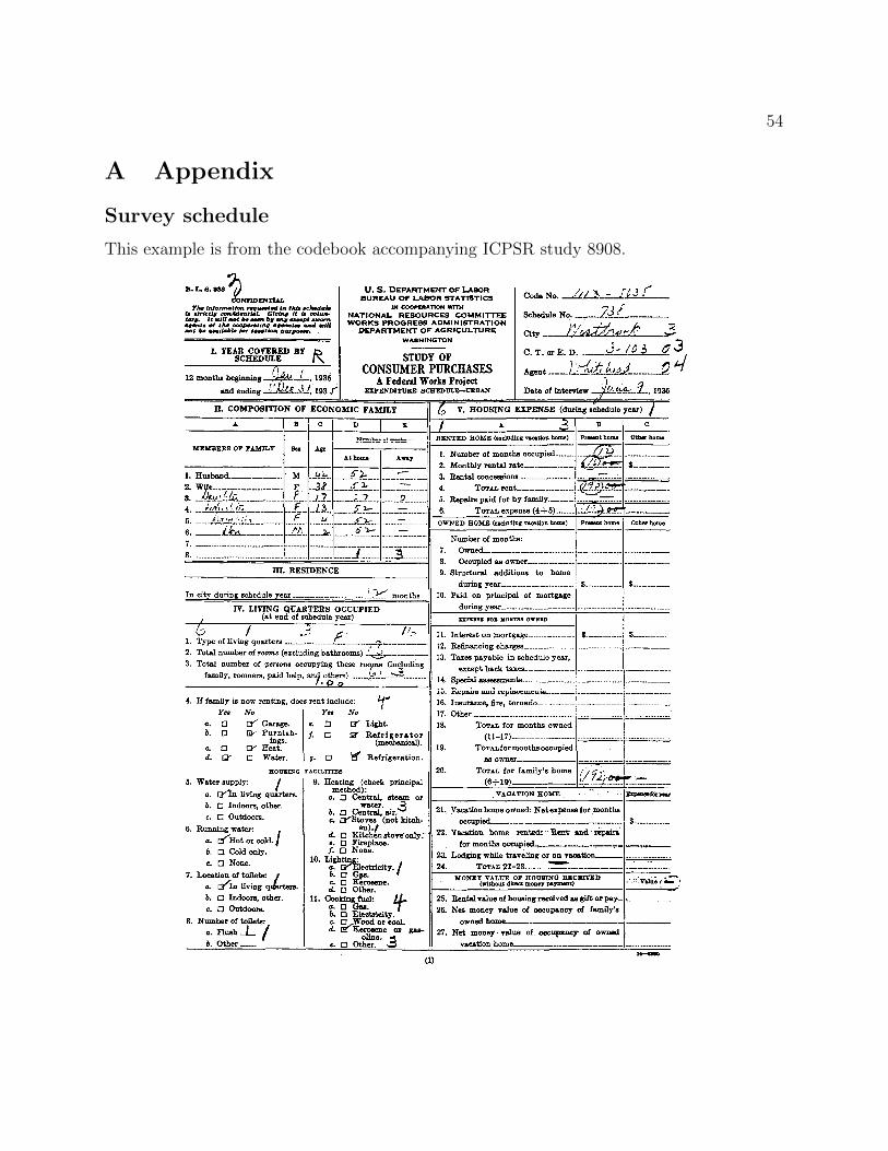
54

A Appendix

Survey schedule

This example is from the codebook accompanying ICPSR study 8908.

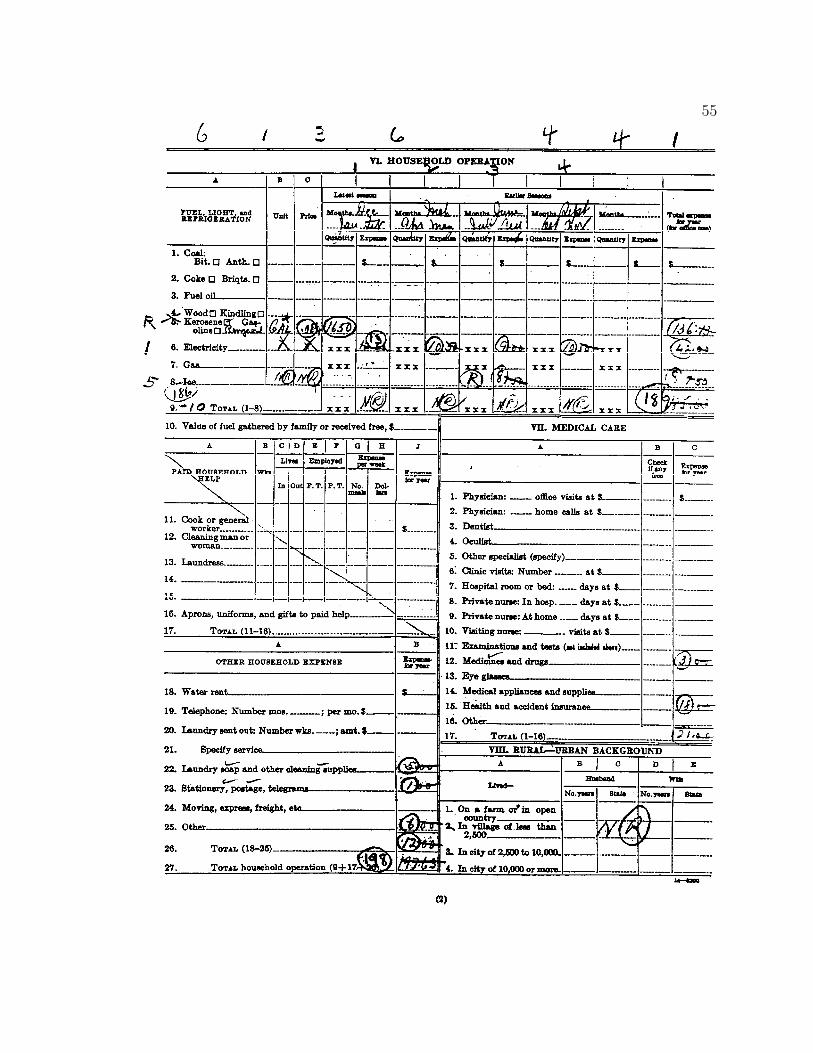
55

56

57

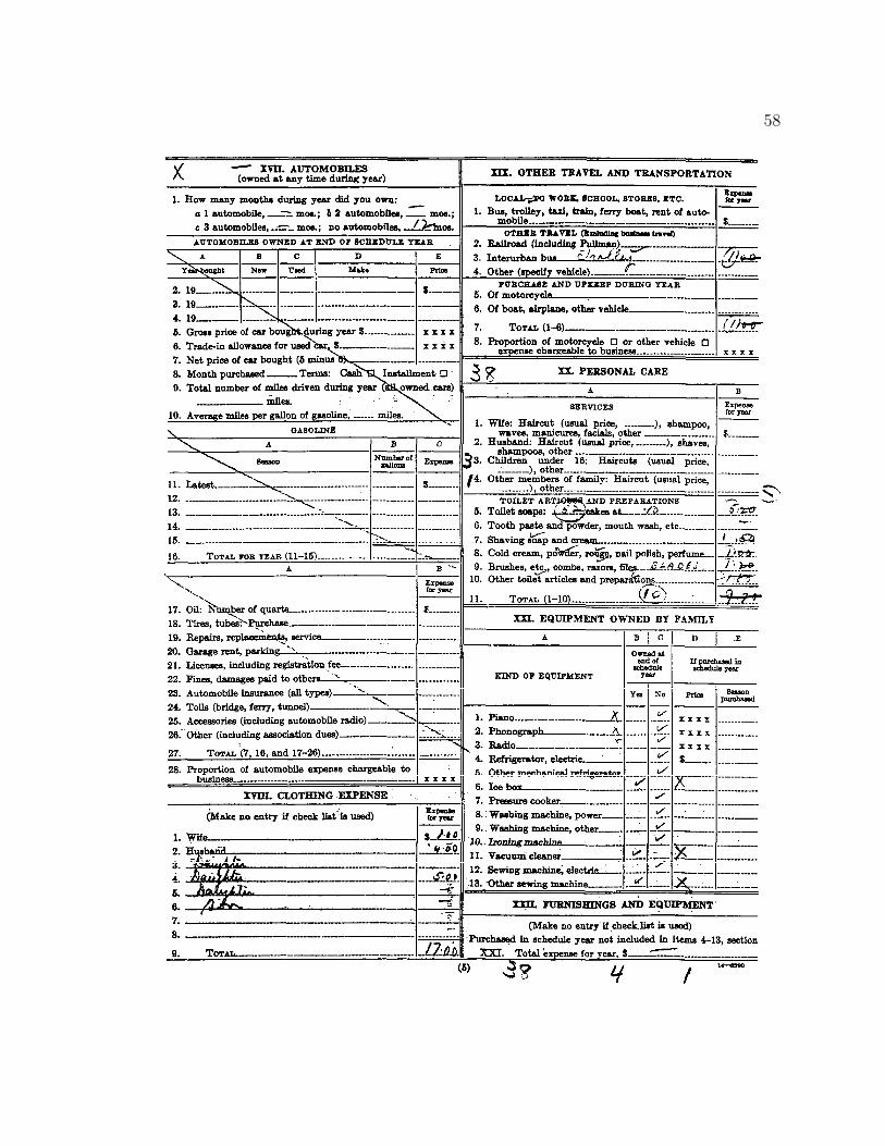
58

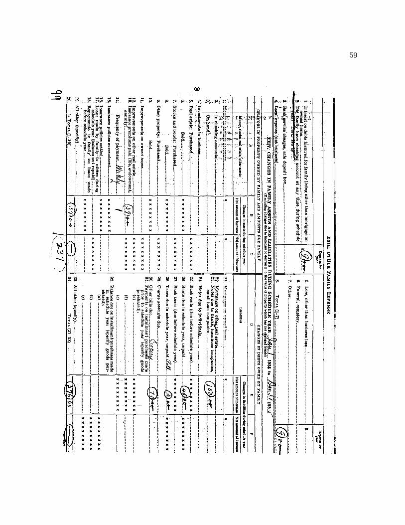
59

60

Measures of consumption calculated from the 1935-36 Study ofConsumer Purchases

Unfortunately, the schedules for the expenditure survey did not include a measure of totalexpenditure; this measure must be built-up from spending on subcategories of consumption.Sometimes the schedule provides a total for a subcategory (like recreation spending). Othertimes, the totals provided on the schedule must be adjusted because they intermingle con-sumption expenditures with non-consumption expenditures. For instance, the total providedfor housing expenditure includes spending on taxes. Below I describe the construction of 16categories of consumption, the sum of which equals total consumer expenditure. Given thestructure of the survey, and the purposes for which I use it, these categories inevitably donot correspond exactly to their NIPA definitions. For example, I exclude the imputed rentalvalue of owner-occupied housing from my measure of consumption.

Housing

Housing expenses are detailed in section V of the urban expenditure schedule. I measureconsumer spending on housing as the sum of rent paid (if renting), spending on repairs tothe house, and spending on home insurance. Also included are expenses for housing whileon vacation.

Specifically, housing is the sum of the following lines in section V of the schedule: line4 + 5 + 15 + 16 + 17 + 21 + 22 + 23. In terms of the variables in the IPCSR dataset,housing equals V359+ V360+ V361+ V362+ V381+ V382+ V383+ V384+ V389+ V390+V385+ V386+ V387.

Household operation

Household operation expenses are detailed in section VI of the schedule. This categoryincludes spending on utilities, paid household help, and postage.

For this variable, I use the total provided on the schedule in section VI, line 27. Thiscorresponds to ICPSR variable V639.

Medical Care

Medical expenses are detailed in section VII of the schedule. This category includes out-of-pocket spending on medical costs as well as spending on health and accident insurance.

For this variable, I use the total provided on the schedule in section VII, line 17. Thiscorresponds to ICPSR variable V686.

Recreation

Spending on recreation is detailed in section IX of the schedule. This category includesspending on movies, games and sports, activities such as camping and skiing, and purchases

61

of radios, musical instruments, children’s toys and other recreational items.For this variable, I use the total provided on the schedule in section IX, line 20. This

corresponds to ICPSR variable V788.

Tobacco

Spending on tobacco is detailed in section X of the schedule. This category includes spendingon cigarettes, cigars, and “smokers’ supplies.”

For this variable, I use the total provided on the schedule in section X, line 5. Thiscorresponds to ICPSR variable V798.

Reading

Spending on reading materials is detailed in section XI of the schedule. This categoryincludes spending on newspapers, magazines, and non-school books.

For this variable, I use the total provided on the schedule in section XI, line 7. Thiscorresponds to ICPSR variable V812.

Education

Spending on education is detailed in section XII of the schedule. This category includesspending on elementary, secondary, and post-secondary education.

For this variable, I use the total provided on the schedule for tuition and supply expenses(section XII, line 10) plus spending on board and room rent at school (lines 11 and 12). Thiscorresponds to ICPSR variables V837 + V838 + V839.

Occupational Expenses (“not reported as business expenses or as deductionfrom gross income”)

Spending on occupational expenses is detailed in section XIII on the schedule. It includesspending on union and professional association dues, technical books, and miscellaneoussupplies and equipment.

For this variable, I use the total provided on the schedule in section XIII, line 6. Thiscorresponds to ICPSR variable V850.

Gifts

Spending on gifts “to persons not members of economic family (not charity)” are reportedin section XV, line 1. This corresponds to ICPSR variable V853.

Food

Spending on food is detailed in section XVI of the schedule. This category includes spendingon food and drink (including alcohol) both at home and away from home.

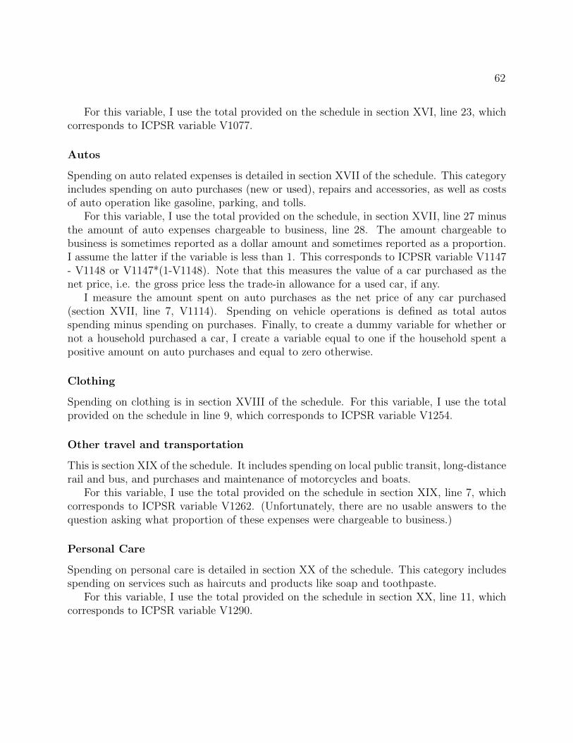
62

For this variable, I use the total provided on the schedule in section XVI, line 23, whichcorresponds to ICPSR variable V1077.

Autos

Spending on auto related expenses is detailed in section XVII of the schedule. This categoryincludes spending on auto purchases (new or used), repairs and accessories, as well as costsof auto operation like gasoline, parking, and tolls.

For this variable, I use the total provided on the schedule, in section XVII, line 27 minusthe amount of auto expenses chargeable to business, line 28. The amount chargeable tobusiness is sometimes reported as a dollar amount and sometimes reported as a proportion.I assume the latter if the variable is less than 1. This corresponds to ICPSR variable V1147- V1148 or V1147*(1-V1148). Note that this measures the value of a car purchased as thenet price, i.e. the gross price less the trade-in allowance for a used car, if any.

I measure the amount spent on auto purchases as the net price of any car purchased(section XVII, line 7, V1114). Spending on vehicle operations is defined as total autosspending minus spending on purchases. Finally, to create a dummy variable for whether ornot a household purchased a car, I create a variable equal to one if the household spent apositive amount on auto purchases and equal to zero otherwise.

Clothing

Spending on clothing is in section XVIII of the schedule. For this variable, I use the totalprovided on the schedule in line 9, which corresponds to ICPSR variable V1254.

Other travel and transportation

This is section XIX of the schedule. It includes spending on local public transit, long-distancerail and bus, and purchases and maintenance of motorcycles and boats.

For this variable, I use the total provided on the schedule in section XIX, line 7, whichcorresponds to ICPSR variable V1262. (Unfortunately, there are no usable answers to thequestion asking what proportion of these expenses were chargeable to business.)

Personal Care

Spending on personal care is detailed in section XX of the schedule. This category includesspending on services such as haircuts and products like soap and toothpaste.

For this variable, I use the total provided on the schedule in section XX, line 11, whichcorresponds to ICPSR variable V1290.

63

Equipment

This corresponds to section XXI on the expenditure schedule and to the total from a separatefurniture and equipment checklist. Nearly all furniture and appliances are included in thiscategory, for instance, refrigerators, washing machines, and lawn mowers. This category alsoincludes spending on household linens and kitchen supplies (silverware, pots, china, and soon).

For this variable I use the total from the check list, if available. This is line 98, columnD, ICPSR V2868. If the total from the checklist is missing, as is true in 570 cases, I use thetotal of all the lines in section XXI (lines 4-13). This corresponds to the ICPSR variablesV1298 + V1301 + V1304 + V1307 + V1310 + V1313 + V1315 + V1318 + V1321 + V1324.

Other

This corresponds to section XXIII on the schedule. In my measure of consumption I includebank service charges (line 3, V1336), non-business legal expenses (line 4, V1337), funeraland cemetery costs (line 6, V1339), and miscellaneous other expenses (line 7, V1340).

Consistency of the household survey two-step estimator

Define variables as follows: Yi is consumption of household i; X1i is a dummy variable equalto 0 if a household was surveyed before the bonus payment (i.e. before June 1936) and equalto 1 if surveyed after; X2i is a dummy variable equal to 1 if the husband in the household isa veteran and 0 if not; Z equals a set of control variables for age, geographic location, andrace (including a constant).

The goal is to obtain a consistent estimate of β3 in

Yi = β1X1i + β2X2i + β3(X1iX2i) + Z ′iβ4 + εi. (A.1)

Since X2i (veteran status) is unobserved in the household survey, I proxy for it by estimating

X2j = Z ′jγ + υj (A.2)

Note the subscripts j rather than i in the second regression, since it is estimated on a sepa-rate sample from (A.1). I will show that given a set of reasonable assumptions, estimationof (A.1) and (A.2) by OLS provides a consistent estimate of β3.

Assumptions

1. E[Ziεi] = 0. This assumption says that age, race, and location are exogenous inequation A.1.

2. E[X1iεi] = 0. This says that whether one was surveyed before or after June 1936 isexogenous in equation A.1.

64

3. E[Ziυi] = 0, i.e. the errors in the first stage are uncorrelated with the control variables.This is true by the properties of OLS. Note that it is because of this condition that thefirst stage must be estimated with OLS rather than with a probit or logit. Althougha probit or logit model would provide better predictions of the probability that ahousehold includes a veteran, the residuals would not necessarily be uncorrelated withthe control variables.

4. X1i is independent of Zi and X2i. This amounts to assuming that households wererandomly assigned to be interviewed before or after June 1936. While not literallytrue, this assumption is reasonable. There is no significant correlation in the databetween observables like age and race and when the household was surveyed.

5. γ is the same in both samples. This is perhaps the strongest assumption; it meansassuming that the true relationship between the control variables (age, race, location)and veteran status is the same in the 1930 census and in the 1936 household survey.In order to come as close as possible to satisfying this assumption, I estimate the firststage on a sample from the 1930 Census that closely matches the sample of householdsin the household survey. For instance, in the first stage I include only married menliving in urban areas.

6. The samples are independent.

Sketch of proofRewrite A.1 substituting in A.2:

Yi = β1X1i + Z ′i[(γ + γ − γ)β2 + β4] + β3X1iZ′i(γ + γ − γ) + β2υi + β3X1iυi + εi

= β1X1i + Z ′i(γβ2 + β4) + β3X1iZ′iγ + ε, (A.3)

where ε = β2Z′i(γ − γ) + β3X1iZ

′i(γ − γ) + β2υi + β3X1iυi + εi.

Let X be the right-hand-side variables in equation A.3, i.e. X ′ = X ′1(X1Zγ)′

Z ′

and let β be the vector of identifiable coefficients, i.e. β is the k by 1 vector β1

β2γ + β4

β3

Then the estimates from my two-stage least squares procedure, β2s, are equal to

= (X ′X)−1X ′Y

= (X ′X)−1X ′(Xβ + ε)

= β + (X ′X)−1X ′ε. (A.4)

65

My procedure will provide a consistent estimate of β if the probability limit of (X ′X)−1X ′εis zero. To show that this is true, I show that each element of X is uncorrelated with the ε.

1. First note that by assumption (5) and the properties of OLS, as the size of the second(census) sample goes to infinity, γ converges in probability to γ, so plim ε = plim β2υi+β3X1iυi + εi. This result will be used in each step that follows.

2. Noting that since X1i is a dummy variable, X21i = X1i

cov(X1i, εi) = (β2 + β3)cov(X1i, υi) + cov(X1i, εi) (A.5)

By assumption (4) the first term on the right hand side equals zero, and by assumption(2) the second term equals zero.

3. Again using the fact that X21i = X1i,

cov(X1iZ′iγ, εi) = cov(X1iZ

′iγ, β2υi) + cov(X1iZ

′iγ, β3X1iυi) + cov(X1iZ

′iγ, εi)

= (β2 + β3)E[X1iZ′iγυi] + E[X1iZ

′iγεi]

= (β2 + β3)E[X1i]E[Z ′iγυi] + E[X1i]E[Z ′iγεi] (A.6)

The last line uses assumption (4), the fact that X1i is independent of Zi and X2i. Thefirst term of (A.6) is zero by assumptions (3) and (6), and the second term is zero byassumption (1).

4. Finally,cov(Zi, ε) = β2cov(Zi, υi) + β3cov(Zi, X1iυi) + cov(Zi, εi) (A.7)

Assumption (3) means the first term on the right hand side is zero; assumptions (3)and (4) make the second term zero, and assumption (1) means the last term is zero.

Thus plim 1NX ′ε is zero, and plim β2s = β. Given assumptions 1-6, two-stage least

squares provides consistent estimates of β.Of course, the two-step procedure means that the standard OLS standard errors will be

incorrect. Because of this, I compute bootstrap standard errors; see section 1.3.

Strata

According to the Bureau of Labor Statistics (1941a, p. 372)

The cities included in the Consumer Purchases Study were chosen to representthe metropolis, the large city with a population from 250,000 to 300,000, themiddle-sized city with a population from 35,000 to 70,000, and the small citywith a population of from 10,000 to 20,000.

66

Large and middle sized cities were selected from each of 6 regions: Northeast, Southeast,East Central, West Central, Rocky Mountain, and Pacific Northwest. In addition, the two‘metropolises’ New York, and Chicago were included, as were several small cities in thenortheast and east central regions.

To avoid problems with strata of 1 sampling unit, I collapse these 15 region-city-sizestrata into 9. This is conservative, since having more strata reduces standard errors (Deaton1997). Table A.1 shows this classification.

Table A.1: Strata classification

City Region Size classification Strata assignment

Aberdeen-Hoquiam, WA Pacific Northwest Middle-sized Pacific Northwest - largeAlbany, GA Southeast Small Southeast - smallAtlanta, GA Southeast Large Southeast - largeBeaver Falls, PA East Central Small East Central - smallBellingham, WA Pacific Northwest Middle-sized Pacific Northwest - largeButte, MT Rocky Mountain Middle-sized Rocky Mountain - largeChicago, IL East Central Large (metropolis) East Central - largeColumbia, SC Southeast Middle-sized Southeast - largeColumbus, OH East Central Large East Central - largeConnellsville, PA East Central Small East Central - smallCouncil Bluffs, IA/Omaha, NE West Central Large West Central - largeDenver, CO Rocky Mountain Large Rocky Mountain - largeDubuque, IA West Central Middle-sized West Central - largeEverett, WA Pacific Northwest Middle-sized Pacific Northwest - largeGastonia, NC Southeast Small Southeast - smallGreenfield, MA Northeast Small Northeast - smallHaverhill, MA Northeast Middle-sized Northeast - largeLogansport, IN East Central Small East Central - smallMattoon, IL East Central Small East Central - smallMobile, AL Southeast Middle-sized Southeast - largeMuncie, IN East Central Middle-sized East Central - largeNew Britain, CT Northeast Middle-sized Northeast - largeNew Castle, PA East Central Middle-sized East Central - largeNew York, NY Northeast Large (metropolis) Northeast - largePeru, IN East Central Small East Central - smallPortland, OR Pacific Northwest Large Pacific Northwest - largeProvidence, RI Northeast Large Northeast - largePueblo, CO Rocky Mountain Middle-sized Rocky Mountain - largeSpringfield, IL East Central Middle-sized East Central - largeSpringfield, MO West Central Middle-sized West Central - largeWallingford, CT Northeast Small Northeast - smallWestbrook, ME Northeast Small Northeast - smallWillimantic, CT Northeast Small Northeast - small

67

Chapter 2

What was Bad for GM was Bad forAmerica: The Automobile Industryand the 1937-38 Recession

2.1 Introduction

The 1937-38 recession is prominent in economists’ accounts of the interwar period and incurrent macro policy debates. After growing rapidly between 1933 and 1937, the U.S. econ-omy plunged back into recession. From 1937 to 1938, real GDP fell 3.5 percent and thenonfarm unemployment rate rose 6.6 percentage points.1 Because the recession was brief,annual numbers disguise the downturn’s severity. Industrial production fell 32 percent be-tween May 1937 and May 1938. This contrasts with a peak to trough industrial productiondecline in the recent U.S. recession of 17 percent.2

Economists typically take the 1937-38 recession as a lesson in the perils of reversingexpansionary monetary and fiscal policy too soon. In June 2009, Christina Romer wrotea column for The Economist on “The Lessons of 1937.” In January 2010, Paul Krugmanwrote a New York Times column entitled “That 1937 Feeling.” Both Romer and Krugmancautioned that a decline in government spending or shrinking of the Federal Reserve’s balancesheet could push the economy back into recession. Their arguments reflect a near-consensusin the academic literature that the 1937-38 recession was caused by contractionary monetarypolicy, fiscal policy, or both (Eggertsson and Pugsley 2006, Eichengreen 1992, Friedman andSchwartz 1963, Romer 1992, Velde 2009, Irwin 2011).3 Both the monetary and fiscal shockhad multiple sources. The Federal Reserve raised reserve requirements in August 1936 and

1Real GDP data are from National Income and Product Accounts (NIPA) table 1.1.6a. The nonfarmunemployment rate is from Lebergott (1964) table A-3. Including the entire labor force, the unemploymentrate rose from 14.3 to 19.1 percent, or, if federal work-relief workers are counted as employed, from 9.2 to12.5 percent (Darby 1976, table 3).

2Industrial production data from FRED series INDPRO.3A prominent exception is Cole and Ohanian (2001). See section 2.2.

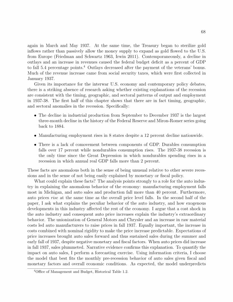
68

again in March and May 1937. At the same time, the Treasury began to sterilize goldinflows rather than passively allow the money supply to expand as gold flowed to the U.S.from Europe (Friedman and Schwartz 1963, Irwin 2011). Contemporaneously, a decline inoutlays and an increase in revenues caused the federal budget deficit as a percent of GDPto fall 5.4 percentage points.4 Outlays decreased after the payment of the veterans’ bonus.Much of the revenue increase came from social security taxes, which were first collected inJanuary 1937.

Given its importance for the interwar U.S. economy and contemporary policy debates,there is a striking absence of research asking whether existing explanations of the recessionare consistent with the timing, geographic, and sectoral patterns of output and employmentin 1937-38. The first half of this chapter shows that there are in fact timing, geographic,and sectoral anomalies in the recession. Specifically:

• The decline in industrial production from September to December 1937 is the largestthree-month decline in the history of the Federal Reserve and Miron-Romer series goingback to 1884.

• Manufacturing employment rises in 8 states despite a 12 percent decline nationwide.

• There is a lack of comovement between components of GDP. Durables consumptionfalls over 17 percent while nondurables consumption rises. The 1937-38 recession isthe only time since the Great Depression in which nondurables spending rises in arecession in which annual real GDP falls more than 2 percent.

These facts are anomalous both in the sense of being unusual relative to other severe reces-sions and in the sense of not being easily explained by monetary or fiscal policy.

What could explain these facts? The analysis points strongly to a role for the auto indus-try in explaining the anomalous behavior of the economy: manufacturing employment fallsmost in Michigan, and auto sales and production fall more than 40 percent. Furthermore,auto prices rise at the same time as the overall price level falls. In the second half of thepaper, I ask what explains the peculiar behavior of the auto industry, and how exogenousdevelopments in this industry affected the rest of the economy. I argue that a cost shock inthe auto industry and consequent auto price increases explain the industry’s extraordinarybehavior. The unionization of General Motors and Chrysler and an increase in raw materialcosts led auto manufacturers to raise prices in fall 1937. Equally important, the increase incosts combined with nominal rigidity to make the price increase predictable. Expectations ofprice increases brought auto sales forward and thus sustained sales during the summer andearly fall of 1937, despite negative monetary and fiscal factors. When auto prices did increasein fall 1937, sales plummeted. Narrative evidence confirms this explanation. To quantify theimpact on auto sales, I perform a forecasting exercise. Using information criteria, I choosethe model that best fits the monthly pre-recession behavior of auto sales given fiscal andmonetary factors and overall economic conditions. As expected, the model underpredicts

4Office of Management and Budget, Historical Table 1.2.

69

sales in the summer of 1937, when consumers expected auto prices soon to increase, andoverpredicts sales in 1938. I interpret the difference between predicted and actual sales asthe impact of the auto sector supply shock.

This exercise implies that without the auto shock, the fall in auto sales between 1937 and1938 would have been 0.8 million rather than the actual 1.6 million. Using data on the priceof cars sold and an estimate of the multiplier, I find that positive price expectations added0.3 percent to GDP in 1937, while the subsequent drop-off in sales subtracted 1.0 percentfrom GDP in 1938: absent the shock, the output decline in 1938 would have been more thana third smaller.

In the final section of the chapter I explore how the auto shock contributed to the reces-sion’s anomalies. I use an unpublished 38x38 input-output table for the 1939 U.S. economyconstructed by Wassily Leontief to quantify the links between the motor vehicle industry andother sectors. Using this information, I provide suggestive evidence that the auto industryshock contributed to the rapid decline in industrial production in fall 1937 and to the longleft tail of negative state employment growth. I also suggest that the auto shock may resolvemuch of the mysterious lack of comovement in the recession. Without this shock, durablesconsumption would have fallen 12 rather than 18 percent. More speculatively, absent therelative price impact of the auto shock, nondurables spending may not have risen, and theremay have been fewer states with positive employment growth.

This chapter contributes to our understanding of the 1937-38 recession by proposingan additional explanation of the recession and by refining our understanding of existingexplanations. It also relates to a long-standing theoretical literature on the importanceof sectoral and firm level shocks for explaining aggregate fluctuations. In particular, itprovides support for Gabaix’s (2011) hypothesis that shocks to large firms may account fora significant portion of aggregate fluctuations.

I proceed in the next section by reviewing the literature on the 1937-38 recession. Section2.3 documents anomalies in the timing, sectoral and geographic incidence of the recession.This motivates section 2.4, which discusses and explains the auto price increase. Section2.5 quantifies the impact on auto sales of the supply shock by constructing a forecast forthe path of auto sales had sales only been impacted by monetary policy, fiscal policy, andthe business cycle. Section 2.6 explores the link between the auto shock and the recession’sanomalies. Section 2.7 concludes and suggests that acknowledging the impact of the autoshock makes monetary and fiscal policy explanations of the remainder of the recession moreplausible.

70

!500

050

010

0015

0020

00M

illion

s of

dol

lars

, n.s

.a.

1936m1 1936m7 1937m1 1937m7 1938m1 1938m7 1939m1 1939m7 1940m1Date

®

Figure 2.1: The Federal budget deficit. Source: NBER macrohistory series m15025c. Un-derlying data from the U.S. Treasury Department, daily treasury statements.

2.2 Previous literature and policy developments

Fiscal Policy

Many authors have placed full or partial blame for the 1937 recession on increasing taxesand decreasing transfers.5 After peaking at 5.5 percent of GDP in fiscal year 1936 (7/1/35-6/30/36), the federal government’s budget deficit shrank to 2.5 percent of GDP in fiscal1937 and 0.1 percent of GDP in fiscal 1938.6 This large swing was divided equally betweenan increase in receipts and a decrease in outlays. Much of the revenue increase came fromsocial security taxes, which began to be collected in January 1937.7 Both workers and firmspaid a one percent payroll tax on the first $3,000 of earnings (Barro and Sahasakul 1986).Corporate tax rates also rose with the enactment of the undistributed profits tax in June1936. Federal government transfers fell after the payment of the veterans’ bonus in thesummer of 1936.

5See, for example, Lewis (1949), Roose (1954), and, more recently, Eichengreen (1992), Romer (1992),and Velde (2009).

6Office of Management and Budget, Historical Table 1.2.7Total federal government receipts rose from 3.923 billion in fiscal 1936 to 6.751 billion in fiscal 1938.

53 percent of this revenue increase is accounted for by social insurance taxes, a category that included bothsocial security taxes and railroad retirement receipts. See Office of Management and Budget, HistoricalTables 2.1 and 2.4.

71

Figure 2.1 shows the monthly federal budget deficit between 1936 and 1939.8 It makesclear the significance of the veterans’ bonus. In June 1936, the federal government paidveterans cash and bonds worth roughly 2 percent of GDP. Not only was this payment toveterans enormous, the previous chapter argues that it was mostly spent in 1936.

Monetary Policy

Along with fiscal policy, the most popular explanation for the 1937-38 recession is restrictivemonetary policy.9 The Federal Reserve raised reserve requirements in August 1936 and againin March and May 1937. In December 1936, the Treasury began sterilizing gold inflows.Friedman and Schwartz argue (1963, pp. 544-545):

The combined impact of the rise in reserve requirements and–no less important–the Treasury gold-sterilization program first sharply reduced the rate of increasein the money stock and then converted it into a decline. . . . The sharp retar-dation in the rate of growth of the money stock must surely have been a factorcurbing expansion, and the absolute decline, a factor intensifying contraction.

Figure 2.2 shows the behavior of the money supply (currency held by the public plusdemand and time deposits of commercial banks) from 1936-1939. The money stock plateausin the spring and summer of 1937 and then declines in the fall. There is an emergingconsensus that the key shock was the Treasury gold sterilization rather than the increase inreserve requirements. Calomiris, Mason, and Wheelock (2011) use individual bank data toinvestigate how tighter reserve requirements affected bank behavior. They find no evidencethat the changes in reserve requirements affected bank reserve demand in 1936-37. Irwin(2011) examines the time series of the deposit-reserve ratio and cannot detect an impactof the reserve requirement changes. By contrast, Irwin argues that gold sterilization hadquantitatively large impacts on the monetary base and thus on the money supply. Heestimates that absent gold sterilization, in 1937 the monetary base would have been as muchas 10 percent larger. However, the channel through which money supply declines impactedreal activity in 1937-38 is unclear. There was relatively little impact on interest rates. Figure2 shows the path of the yield on three-month treasury bills. Although yields briefly spike by10 to 40 basis points in the spring and summer of 1937, they remain close to zero over theperiod. Other interest rates rose only slightly. For example, in 1937 the prime commercialpaper rate rose from 0.75 to 1 percent (Irwin 2011).

Of course when interest rates are near zero, monetary policy can still change expectationsof inflation and thus affect the real interest rate and the real economy. This is the channelthrough which Romer (1992) argues that money supply growth led to economic recovery after

8Monthly budget deficit figures are derived from daily treasury statements and reported in NBER macro-history series m15025c.

9See, for example, Roose (1954), Friedman and Schwartz (1963), Eichengreen (1992), Romer (1992),Velde (2009), and Irwin (2011).

72

!one% 'uppl% (le,t a/is)

3!month 6reasur% 8ield (ri:ht a/is)

020

40>0

8010

0Aa

sis

Poin

ts

4045

5055

D bi

llions

F sGa

G

193>m1 1937m1 1938m1 1939m1 1940m1Date

®

Figure 2.2: The money supply and 3-month treasury yield. The money supply is currencyheld by the public + demand and time deposits of commercial banks. Sources: NBERmacrohistory series 1444a; FRED series TB3MS.

1933. Eggertsson and Pugsley (2006) argue that policymakers’ actions in the spring of 1937lowered inflation expectations, and through this channel, caused the 1937-1938 recession.This provides one way of explaining how monetary actions, despite little impact on interestrates, may have had large real effects.

Unionization

Cole and Ohanian (2001, 2009) argue that New Deal policies and unionization led to highwages in manufacturing and a slow recovery of output and employment after 1933. Theybriefly suggest that a spike in wages due to the upholding by the Supreme Court of theNational Labor Relations Act (the Wagner Act) in April 1937 contributed to the 1937-38recession. Since this is not the focus of their work, they provide no quantitative evidence - be-yond the documentation of wage increases - for this effect. My work supports their argumentinsofar as it shows how unionization in the automobile industry did substantially contributeto the recession. The transmission mechanism in my paper is, however, different from that inCole and Ohanian. I argue that unionization had large impacts in the auto industry becauseit affected expectations of the future price of automobiles, leading to substantial intertem-poral substitution of auto purchases. Furthermore, whereas Cole and Ohanian suggest thatwage increases induced by unionization were the primary cause of the recession, I argue thatunderstanding the auto industry shock and its contributions to the recessions’ anomalies

73

may in fact strengthen the case for monetary and fiscal policy explanations of the recession.

2.3 Anomalies

Timing

The NBER dates the business cycle peak as May 1937. During the summer, however, pro-duction and employment declined only slightly. Indeed, Romer’s (1994) business cycle datingalgorithm selects August as the peak. The period between May and August was marked bya decoupling of nondurable and durable goods manufacturing. Nondurables peaked in May,with production falling by 6.1 percent over the ensuing three months. Durables productionrose 3.7 percent over the same period, peaking in August.10

In early fall, the character of the recession changed entirely. Seasonally adjusted indus-trial production fell 24 percent from September to December 1937. The decline in outputwas accompanied by large declines in employment. From September 1937 to January 1938,22 percent of durable goods employment - 917,000 jobs - disappeared.11 These job losseswere reflected in a rapidly rising unemployment rate. The monthly series from the Na-tional Industrial Conference Board shows the unemployment rate rising from 11.6 percentin September 1937 to 16.9 percent in January 1938.12

Figure 2.3 shows the path of industrial production around the business cycle peak in1937, and, for comparison, in 1920 and 1929. It makes clear how extraordinarily rapidthe contraction was in 1937. Indeed, the decline in industrial production from September toDecember 1937 is the largest three-month decline in the history of the Federal Reserve Boardseries (which begins in 1919), and is larger than any three-month decline in the Miron-Romerseries that goes back to 1884.

I am unaware of any existing work that emphasizes or offers explanations for the speed ofthe economy’s collapse in fall 1937. Existing theories of the recession are unpromising in thisregard. The timing of the decrease in transfers (the second half of 1936) or the increase intaxes (the beginning of 1937) fits poorly with the rapid economic decline in the fall of 1937.Theory and evidence suggest that changes in taxes and transfers should have immediateimpacts. Parker et al. (2011), for instance, find that the largest impact of the 2008 stimuluspayments was in the quarter of payment.13 The decline in the money supply in 1937 wassmall compared to that in the Great Depression and is thus ill-suited to explain a much morerapid decline in industrial production. Finally, the collapse in production occurred 6 monthsafter April 1937, the key date in Cole and Ohanian’s supply shock story.

10Seasonally adjusted data are from the Federal Reserve Bulletin, August 1940, p. 765.11Factory employment data are from the Federal Reserve Bulletin, October 1939.12NBER macrohistory series m08292a.13Using a structural VAR, Blanchard and Perotti (2002) also find that output declines in the quarter in

which taxes rise, however, they find that the peak impact on output occurs 5-7 quarters after a tax shock,a result more consistent with the 1937-38 experience.

74

7080

9010

0N

BER

Pea

k=10

0

-10 -5 0 5 10 15Months before / after NBER peak

Aug. '29 May '37Dec. '07

Figure 2.3: Seasonally adjusted industrial production around business cycle peaks in 1920,1929, and 1937. Source: Industrial production is the seasonally adjusted Fed index, FREDseries INDPRO.

Geography

A generally unappreciated aspect of the 1937-38 recession was its varying impact acrossstates.14 Figures 2.4 and 2.5 show the percent change in private nonfarm and manufacturingemployment between 1937 and 1938. Despite a 5 percent decline in the country as a whole,total private employment rose in 11 states. Perhaps more remarkably, while manufacturingemployment fell 12 percent nationwide, it rose in 8 states. Of course, recessions always effectsome states more than others. States have different concentrations of cyclically sensitiveindustries and different pre-recession employment trends. But it is unclear how these factorscan explain actual increases in employment in some states during a severe recession. Andthere is strong evidence that the degree of geographic dispersion in 1937-38 was unusualrelative to other interwar downturns.

Tables 2.1 and 2.2 compare the variation in the change in private and manufacturingemployment between 1937 and 1938 with that between 1929 and 1932. In the case ofmanufacturing, it is also possible to extend the comparison to 1919-21. The tables show aremarkably consistent story: in each year of the initial downturn from 1929-32, the coefficientof variation is close to or less than 0.5, and employment rises in no more than 2 states. Bycontrast, in 1937-38, the coefficient of variation is over 1 and employment rises in many

14An exception is Wallis (1989, p. 61) who notes the “markedly differential regional impact” of the1937-38 recession but does not compare the geographic variation to that in other interwar downturns.

75

Figure 2.4: Change in private nonfarm payroll employment, 1937-38 (%). Source: Wallis(1989).

Figure 2.5: Change in manufacturing employment, 1937-38 (%). Source: Wallis (1989).

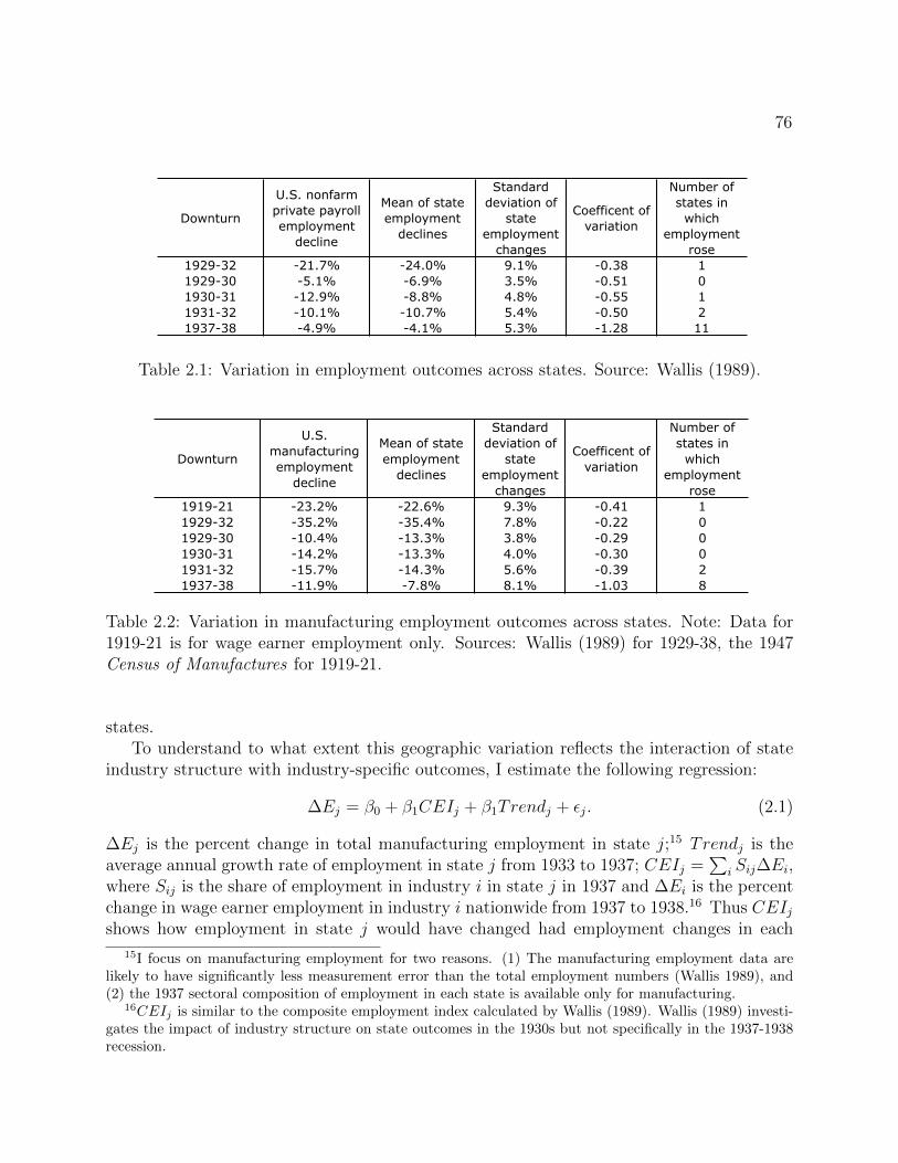
76

Downturn

U.S. nonfarm

private payroll

employment

decline

Mean of state

employment

declines

Standard

deviation of

state

employment

changes

Coefficent of

variation

Number of

states in

which

employment

rose

1929-32 -21.7% -24.0% 9.1% -0.38 1

1929-30 -5.1% -6.9% 3.5% -0.51 0

1930-31 -12.9% -8.8% 4.8% -0.55 1

1931-32 -10.1% -10.7% 5.4% -0.50 2

1937-38 -4.9% -4.1% 5.3% -1.28 11

Table 2.1: Variation in employment outcomes across states. Source: Wallis (1989).

Downturn

U.S.

manufacturing

employment

decline

Mean of state

employment

declines

Standard

deviation of

state

employment

changes

Coefficent of

variation

Number of

states in

which

employment

rose

1919-21 -23.2% -22.6% 9.3% -0.41 1

1929-32 -35.2% -35.4% 7.8% -0.22 0

1929-30 -10.4% -13.3% 3.8% -0.29 0

1930-31 -14.2% -13.3% 4.0% -0.30 0

1931-32 -15.7% -14.3% 5.6% -0.39 2

1937-38 -11.9% -7.8% 8.1% -1.03 8

Table 2.2: Variation in manufacturing employment outcomes across states. Note: Data for1919-21 is for wage earner employment only. Sources: Wallis (1989) for 1929-38, the 1947Census of Manufactures for 1919-21.

states.To understand to what extent this geographic variation reflects the interaction of state

industry structure with industry-specific outcomes, I estimate the following regression:

∆Ej = β0 + β1CEIj + β1Trendj + εj. (2.1)

∆Ej is the percent change in total manufacturing employment in state j;15 Trendj is theaverage annual growth rate of employment in state j from 1933 to 1937; CEIj =

∑i Sij∆Ei,

where Sij is the share of employment in industry i in state j in 1937 and ∆Ei is the percentchange in wage earner employment in industry i nationwide from 1937 to 1938.16 Thus CEIjshows how employment in state j would have changed had employment changes in each

15I focus on manufacturing employment for two reasons. (1) The manufacturing employment data arelikely to have significantly less measurement error than the total employment numbers (Wallis 1989), and(2) the 1937 sectoral composition of employment in each state is available only for manufacturing.

16CEIj is similar to the composite employment index calculated by Wallis (1989). Wallis (1989) investi-gates the impact of industry structure on state outcomes in the 1930s but not specifically in the 1937-1938recession.

77

Dependent variable is percent change in state manufacturing employment 1937-38 (average decline is 7.8%)

CEI 1.721*** 1.295*** 1.576*** 1.668***

(0.192) (0.279) (0.211) (0.318)

Impact of 1 standard deviation

increase (percentage points) 6.5 4.9 5.1 5.4

33-37 growth -1.318*** -0.488** -1.167*** 0.132

(0.191) (0.239) (0.312) (0.335)

Impact of 1 standard deviation

increase (percentage points) -5.8 -2.1 -3.6 0.4

Constant 3.194* 17.66*** 15.44*** 0.658 15.40*** 15.69***

(1.799) (2.924) (3.030) (3.005) (3.470) (3.597)

Sample

Observations 48 48 48 31 31 31

R-squared 0.509 0.637 0.668 0.325 0.658 0.659

Standard errors in parentheses

*** p<0.01, ** p<0.05, * p<0.1

All StatesStates with > 50,000 wage earners

in manufacturing

Table 2.3

industry in the state exactly matched the nationwide changes in employment by industry.17

Put differently, variation in CEIj across states reflects only differences in industry structureacross states. To compute state shares of employment by industry, I collected data onemployment in every industry by state from the 1937 Census of Manufactures. Data onnationwide changes in employment by industry were taken from the October 1939 FederalReserve Bulletin.

Table 2.3 shows results both for all states and for the 31 states with more than 50,000wage earners in manufacturing in 1937.18 The measure of industry structure, CEI, and toa lesser extent, trend growth in the state from 1933 to 1937 are robustly statistically andeconomically significant. A one standard deviation decline in CEI is associated with morethan 5 percentage points lower manufacturing employment growth. Measured by the R2,CEI alone explains nearly 2/3 of the variation in state employment changes. The negativecoefficient on 1933-37 growth means that on average states that grew faster after 1933 didworse in the 1937-38 recession. However, this result disappears when the measure of industrystructure is included in the 31 state sample.

Industry structure’s overwhelming importance suggests that the geographic anomalies in1937-38 are primarily a manifestation of an unusual pattern of output movements acrossindustries.19 To understand why state outcomes were so different in 1937-38, one must

17This statement is approximate, since the left hand side variable of the regression is total manufacturingemployment, while data limitations force me to compute CEIj using data on wage earner employment only.

18Data on the number of manufacturing wage earners in each state come from the 1937 Census of Man-ufactures.

19Existing explanations of the recession also suggest possible factors that could have directly caused

78

understand sectoral output patterns in the recession. The next section turns to this topic.

Sectoral

Macroeconomists view comovement as a common element of recessions. There is widespreaddisagreement about the causes of particular recessions, but there is a widespread agreementthat recessions are not simply the result of dramatic declines in output in one sector ofthe economy. Rather they are events in which nearly all sectors decline, albeit to differentdegrees. Long and Plosser (1987) summarize this conventional view, stating: “Comovementamong a wide variety of economic activities is an essential empirical characteristic of businesscycles” (p. 333). This view of business cycles has shaped nearly all macroeconomic models.Models ranging from old Keynesian to real business cycle are constructed so that negativeshocks lead to declines in output and employment across all forms of consumption andinvestment.

To a surprising degree, the 1937-38 recession does not fit this accepted wisdom. Thefollowing describes movements in components of consumption and investment in 1937-38versus in other recession years.

Consumption

Between 1937 and 1938 real durables consumption fell 17.1 percent. New motor vehiclesconsumption fell 42 percent. This decline in durables, and particularly motor vehicles,consumption was extraordinarily unusual given the behavior of GDP.

The solid line in figure 2.6 shows the median behavior of durables consumption in postwarU.S. recessions. The dashed line shows the behavior in 1937. Of course, given that the declinein GDP is more severe in 1938, we would expect durables to fall more. To adjust for thedecline in GDP, Figure 2.7 shows a scatter plot of the change in durables consumption andthe change in GDP in all years with negative output growth since 1929, excluding 1945-47.

The decline in durables consumption spending in 1938 is anomalous when compared topostwar recessions or to the Great Depression. In postwar recessions, durables consumptionspending has never fallen by more than eight percent in a single year. In 2009, when GDPdeclined by 3.1 percent, just slightly less than the decline in 1938, durables consumption

unusual geographic dispersion in the recession. Insofar as the fiscal shock was due to the beginning of socialsecurity tax collection, states with more workers subject to social security taxes may have fared worse inthe recession (Wallis 1989). Insofar as the monetary shock took the form of a reserve requirement increase,states with a larger percent of bank deposits in Federal Reserve member banks may have suffered more. Andinsofar as general, rather than sector specific, unionization induced wage increases mattered, states withmore workers unionized may have performed worse (Wallis 1989).

To test for the importance of each of these factors, I added proxies for the percent of workers coveredby social security, the share of bank deposits in Federal Reserve member banks, and the union membershiprate to (2.1). None of these variables are robustly economically or statistically significant with the possibleexception of social security coverage. Full results available on request. See also Wallis (1989).

79

6070

8090

100

110

GD

P Pe

ak=1

00

-3 -2 -1 0 1 2 3Years before / after GDP peak

Median 1937

Figure 2.6: Real durables consumption around business cycle peaks, postwar median and1937. Median includes all post World War II business cycles in which annual GDP fell (1948,1953, 1957, 1973, 1980, 1981, 1990, and 2007). Source: NIPA table 1.1.3.

1930

1931

1932

1933

1949

1954

19581974

1975

1980

1982

199120082009

1938

-30

-20

-10

010

Rea

l Dur

able

s C

onsu

mpt

ion

Gro

wth

(%)

-15 -10 -5 0Real GDP Growth (%)

Figure 2.7: Scatter plot of durables consumption growth against GDP growth. Includes allyears of negative GDP growth since 1929, excluding 1945-1947. Source: NIPA table 1.1.3.

80

7080

9010

011

0G

DP

Peak

=100

-3 -2 -1 0 1 2 3Years before / after GDP peak

Median 1937

Figure 2.8: Real household durables consumption around business cycle peaks, postwarmedian and 1937. Median includes all post World War II business cycles in which annualGDP fell (1948, 1953, 1957, 1973, 1980, 1981, 1990, and 2007). Source: NIPA table 2.4.3.

1930

1931

1932

1933

1949

19541958

1974

1975

19801982

1991

2008

20091938

-20

-15

-10

-50

Rea

l Hou

seho

ld D

urab

les

Con

sum

ptio

n G

row

th (%

)

-15 -10 -5 0Real GDP Growth (%)

Figure 2.9: Scatter plot of household durables consumption growth against GDP growth.Includes all years of negative GDP growth since 1929, excluding 1945-1947. Source: NIPAtable 1.1.3 and 2.4.3.

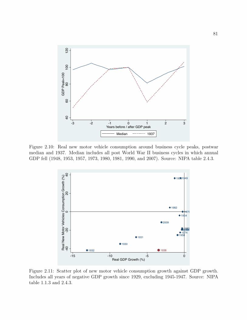
81

4060

8010

012

0G

DP

Peak

=100

-3 -2 -1 0 1 2 3Years before / after GDP peak

Median 1937

Figure 2.10: Real new motor vehicle consumption around business cycle peaks, postwarmedian and 1937. Median includes all post World War II business cycles in which annualGDP fell (1948, 1953, 1957, 1973, 1980, 1981, 1990, and 2007). Source: NIPA table 2.4.3.

1930

1931

1932

19331949

1954

19581974

1975

1980

1982

19912008

2009

1938-40

-20

020

40R

eal N

ew M

otor

Veh

icle

s C

onsu

mpt

ion

Gro

wth

(%)

-15 -10 -5 0Real GDP Growth (%)

Figure 2.11: Scatter plot of new motor vehicle consumption growth against GDP growth.Includes all years of negative GDP growth since 1929, excluding 1945-1947. Source: NIPAtable 1.1.3 and 2.4.3.

82

spending fell by ‘only’ 5.4 percent.20 Many economists have noted and attempted to explainthe 17.2 percent decline in durables consumption in 1930 (Mishkin 1978, Romer 1990, Olney1999). Less noted is the fact that durables spending falls by almost exactly the same amountin 1938 (17.1 percent), despite a decline in output only 40 percent as large.

Figures 2.8-2.11 repeat figures 2.6 and 2.7 for the two largest components of durablesconsumption spending, household durables (including furniture and appliances), and newmotor vehicles. From 1937 to 1938, household durables spending declines by 9.6 percentand new motor vehicles spending falls by 41.5 percent. Figure 2.8 shows that the declinein household durables spending was far larger than in a typical recession, but figure 2.9suggests that given the large decline in GDP, the decline in household durables spendingwas not too unusual. By contrast, the 41.5 percent decline in new motor vehicles spendingwas remarkable (figures 2.10, 2.11) even given the magnitude of the 1938 recession. Sincethe BEA series began in 1929, only one year saw a larger decline in auto spending: in 1932,spending fell by 41.7 percent, 0.2 percentage points more than in 1938. But whereas in 1938real GDP fell 3.5 percent, in 1932 it fell 13.0 percent.21

Nondurables Consumption

The poor performance of durables spending in 1937-38 was matched by unusually strongnondurables spending. From 1937-38, nondurables spending rose by 1.4 percent (figure 2.12).This reflected an increase in real spending on food and beverages of 2.1 percent, an increasein spending on clothing and footwear of 1.4 percent, and a 1.1 percent decline in spendingon energy.22 A scatter plot of changes in GDP and nondurables spending (figure 2.13) showshow unusual it is for nondurables spending to rise during a large recession. The 1937-1938recession is the only time since the Great Depression in which nondurables spending rose ina recession in which annual GDP fell more than 2 percent.

Investment

Economists often expect that consumer durables and investment will behave similarly. Bothought to be sensitive to interest rates and to expectations of future income. To some ex-tent, this intuition holds true in 1937-1938. Business investment - nonresidential structures,equipment, and inventories - does poorly. Oddly, on an annual basis, residential investmentrises in 1938. However, this result is sensitive to the use of annual data. Gordon and Krenn’s(2010) quarterly estimates of residential investment show a 25.4 percent decline in residentialinvestment between the second quarter of 1937 and the second quarter of 1938.23

20NIPA table 1.1.1.21NIPA table 1.1.6a.22NIPA table 2.3.1.23Gordon and Krenn (2010) provide monthly estimates of real GDP components back to 1919. To

construct these estimates, they use the Chow and Lin (1971) interpolation procedure. Monthly interpolatersare chosen from the NBER macrohistory database. For years after 1929, the average of the monthly estimatesis constrained to be equal to the NIPA data. Before 1929, monthly estimates average to the annual data in

83

8090

100

110

GD

P Pe

ak=1

00

-3 -2 -1 0 1 2 3Years before / after GDP peak

Median 1937

Figure 2.12: Real nondurables consumption around business cycle peaks, postwar medianand 1937. Median includes all post World War II business cycles in which annual GDP fell(1948, 1953, 1957, 1973, 1980, 1981, 1990, and 2007). Source: NIPA table 1.1.3.

1930

1931

1932

1933

194919541958

1974

1975

1980

1982

1991

20082009

1938

-8-6

-4-2

02

Rea

l Non

dura

bles

Con

sum

ptio

n G

row

th (%

)

-15 -10 -5 0Real GDP Growth (%)

Figure 2.13: Scatter plot of nondurables consumption growth against GDP growth. Includesall years of negative GDP growth since 1929, excluding 1945-1947. Source: NIPA table 1.1.3.

84

1919-20 1920-21

Perishables 1.9% 6.2%

Semi-Durables -7.5% 9.3%

Durables 2.4% -24.6%

Household appliances 14.2% -38.0%

Motor Vehicles 11.7% -23.2%

Memo: Real GNP -1.1% -2.4%

Change in Real Output of Consumer Goods

Table 2.4: Consumption 1919-21. Sources: Consumption - Shaw (1947); GNP - Romer(1989).

The 1920-21 Recession

The preceding analysis uses data from the National Income and Product Accounts (NIPA)which begin only in 1929. It is also of interest to compare the 1937-38 recession with that in1920-21. Shaw (1947) provides data on commodity output for different components of con-sumption in this period. While not directly comparable to NIPA data, Romer (1989) arguesthat the Shaw data is accurate and unbiased. Table 2.4 shows the behavior of components ofconsumption between 1919 and 1921. Interestingly, as in 1937-38, nondurables consumptionrises between 1920-1921 while durables consumption falls by a large amount. Relative to thedecline in durables consumption as a whole, the decline in auto purchases is, however, notunusually large in 1920-21. Consumption of household appliances falls by significantly morethan that of motor vehicles.

Sectoral behavior and existing theories of the recession

The sectoral pattern of output is not easily explained by any existing theories of the 1937-38recession. Theory and empirics suggest that increases in federal taxes (and decreases intransfers) should decrease all forms of consumption, not only durables consumption. Parkeret al. (2011), for example, find that the economic stimulus payments of 2008 increasednondurables consumption. Despite the attraction of autos to veterans, even the veterans’bonus of 1936 was likely spent on nondurables as well as durables (see the previous chapter).And it is unclear why a monetary policy shock should impact one credit sensitive sector,autos, so much more than other durable goods or housing. Cole and Ohanian’s (2001) union

Gordon and Veitch (1986).The combination of the interpolation procedure and controversy over the correct annual figures for pre-

1929 real GDP suggest that these data must be used with caution. For example, the Gordon and Krenndata show a 5.4 decline in real GDP from 1919-21, whereas Romer (1989) finds a 3.5 percent decline. Andthe Gordon and Krenn real GDP series has a peak in the first quarter of 1929, at odds with the usual viewthat the Great Depression began in the late summer of 1929. For these reasons, in this section I focus onmore standard annual data. However, appendix table 1 provides a quarterly comparison of interwar andpostwar recessions using the Gordon and Krenn data.

85

Price Index Change 1937-38 (%)

GDP -1.9

Consumption (PCE) -2.3

Durables -0.1

Furniture and furnishings -3.2

Household appliances 0.4

New motor vehicles 5.0

Nondurables -4.9

Services 0.1

Private Investment -3.2

Nonres. structures -1.9

Equipment 2.4

Trucks, buses, trailers 12.0

Autos 3.6

Residential 3.2

Exports -4.6

Imports -7.6

Government 0.2

Table 2.5: Prices 1937-38. Source: NIPA tables 1.1.4, 2.4.4., and 5.5.4.

wage shock hypothesis also does not easily explain the disproportionate decline of the autoindustry. If wages rose in many industries, why was the auto industry uniquely affected?

2.4 An auto industry supply shock

The recession’s anomalies strongly point to a role for the auto industry. I have shown thatmanufacturing employment falls most in Michigan and motor vehicle spending falls over 40percent. The mystery is deepened by the fact that auto prices rise in the fall of 1937.

Table 2.5 shows the percent change from 1937 to 1938 in the price indexes for the majorcomponents of GDP. Prices economy-wide (measured by the GDP deflator) fell 1.9 percent.Consumer prices (measured by the personal consumption expenditures deflator) fell 2.3 per-cent. Prices for most sub-categories of output also fell. A notable exception was the price ofautos. Prices of autos purchased by consumers rose 5.0 percent; prices of autos purchasedby businesses increased 3.6 percent. Truck and bus prices rose 12 percent.

Other measures of auto prices confirm a large price spike with the introduction of 1938model year cars in the fall of 1937. According to the BLS wholesale auto price index, nominalauto prices rose by more than 14 percent from December 1936 to December 1937.24 Sincemost prices were falling, this meant that the real price of autos rose by even more. Thisprice increase is more extraordinary when compared to the behavior of auto prices duringthe recovery from 1933-1937. Figure 2.14 shows the path of auto wholesale prices and thePPI. Until fall 1937, nominal auto prices were essentially flat, while economy-wide prices rose

24NBER macrohistory series m04180b.

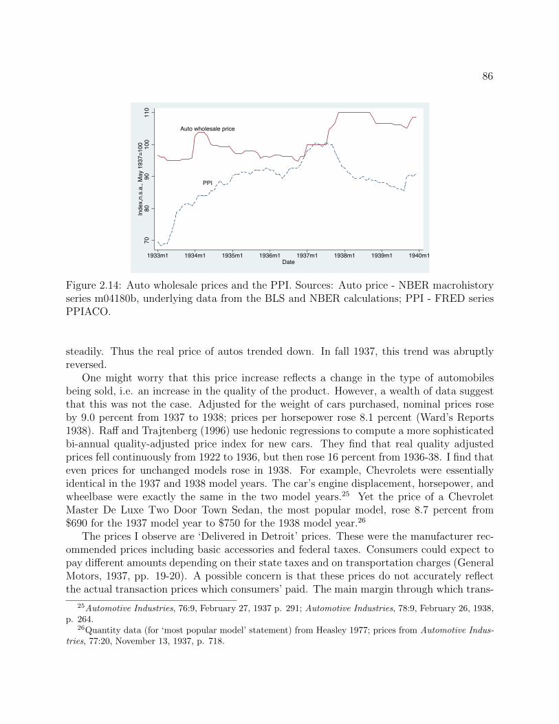
86

PPI

Auto wholesale price

7080

9010

011

0In

dex,

n.s.

a., M

ay 1

937=

100

1933m1 1934m1 1935m1 1936m1 1937m1 1938m1 1939m1 1940m1Date

®

Figure 2.14: Auto wholesale prices and the PPI. Sources: Auto price - NBER macrohistoryseries m04180b, underlying data from the BLS and NBER calculations; PPI - FRED seriesPPIACO.

steadily. Thus the real price of autos trended down. In fall 1937, this trend was abruptlyreversed.

One might worry that this price increase reflects a change in the type of automobilesbeing sold, i.e. an increase in the quality of the product. However, a wealth of data suggestthat this was not the case. Adjusted for the weight of cars purchased, nominal prices roseby 9.0 percent from 1937 to 1938; prices per horsepower rose 8.1 percent (Ward’s Reports1938). Raff and Trajtenberg (1996) use hedonic regressions to compute a more sophisticatedbi-annual quality-adjusted price index for new cars. They find that real quality adjustedprices fell continuously from 1922 to 1936, but then rose 16 percent from 1936-38. I find thateven prices for unchanged models rose in 1938. For example, Chevrolets were essentiallyidentical in the 1937 and 1938 model years. The car’s engine displacement, horsepower, andwheelbase were exactly the same in the two model years.25 Yet the price of a ChevroletMaster De Luxe Two Door Town Sedan, the most popular model, rose 8.7 percent from$690 for the 1937 model year to $750 for the 1938 model year.26

The prices I observe are ‘Delivered in Detroit’ prices. These were the manufacturer rec-ommended prices including basic accessories and federal taxes. Consumers could expect topay different amounts depending on their state taxes and on transportation charges (GeneralMotors, 1937, pp. 19-20). A possible concern is that these prices do not accurately reflectthe actual transaction prices which consumers’ paid. The main margin through which trans-

25Automotive Industries, 76:9, February 27, 1937 p. 291; Automotive Industries, 78:9, February 26, 1938,p. 264.

26Quantity data (for ‘most popular model’ statement) from Heasley 1977; prices from Automotive Indus-tries, 77:20, November 13, 1937, p. 718.

87

Figure 2.15: Advertisement for a 1938 Plymouth. Source:http://www.flickr.com/photos/paulmalon/5744021193/.

action prices could differ was through varying allowances for used car trade-ins (FederalTrade Commission 1939). This concern is mitigated by two facts. First, the delivered inDetroit prices match those published in advertisements, suggesting that they were stronglycorrelated with the actual transaction prices a consumer could expect to pay. Figure 2.15shows an advertisement for a 1938 model year Plymouth sedan. The price on the ad - $685- exactly matches that published in the industry trade journal Automotive Industries onNovember 13, 1937. (The same car cost $620 in the 1937 model year.) The second reasonto believe that transaction prices did indeed rise for the 1938 model year is that industryobservers were unanimous in stating that this was the case (Automotive Industries, fall 1937issues).

Why did auto prices rise?

Auto prices rose because manufacturer’s costs rose. Those in control of the auto industry tookas given that they ought to respond to higher costs by raising prices. For example, AlfredSloan, the CEO of General Motors, said in July 1937 (Automotive Industries, 7/31/37,p. 142): “Naturally, this trend toward rapidly increasing costs must, of necessity reflectitself in the form of a substantial increase in selling prices, with due regard for the effect of

88

volume.” In explaining a planned price increase, a vice-president at Hudson Motor Companysaid (Automotive Industries, 8/14/37, p. 206): “Practically every product entering into themanufacture of our cars, including wages, has risen substantially in price. Naturally, thisaffects the price of our own product.” The increase in costs referred to by these executiveshad two components: a strike / unionization induced wage increase and a raw material priceincrease.

Unionization

Unionization in the auto industry occurred in the context of rapid unionization in many sec-tors.27 The percent of nonagricultural employees organized in unions rose from 13.1 percentin 1935 to 24.5 percent in 1940. Much of this increase was the result of successful effortsby the Congress of Industrial Organizations (the CIO) to organize heavy industry. In 1936,two factors made the automobile industry particularly ripe for unionization. First, workerdiscontent was widespread. One important factor was the seasonal aspect of employment, inwhich workers lost their jobs during the model year changeover with no guarantee that theywould be rehired. Second, the dependence of manufacturers on certain key parts-producingplants made it easy for a strike at one plant to cripple an entire firm.

The United Automobile Workers (UAW), a largely independent affiliate of the CIO, beganits organizing drive in November 1936. A key aspect of their strategy was the sit-down strike,in which workers occupied factories, preventing any production from occurring. The mostimportant sit-down strike began on December 28 and 29 at Fisher body plants in Clevelandand Flint. Fisher body was a division of General Motors, and these plants were crucial linksin the corporation’s supply chain. Halting production at these two plants was sufficient todisrupt three-quarters of General Motor’s total production. Strikes spread to other plants,and by early February, weekly vehicle production at General Motors had declined to 1,500units from 53,000 units in mid-December.

With the help of Frank Murphy, Michigan’s democratic governor, and pressure from Pres-ident Roosevelt, these strikes led to an agreement between the UAW and General Motors onFebruary 11, 1937 in which General Motors agreed to recognize the UAW as a bargainingagent for its members. The agreement itself secured no wage increases, but General Motorsunilaterally increased wages while the sit-down strikes were ongoing. After organizing GM,the UAW organized sit-down strikes at Chrysler and reached a collective bargaining agree-ment on April 6. Despite UAW efforts, however, Ford was not successfully organized until1941. In large part this reflected extreme ideological opposition to unions by Henry Fordand Ford’s willingness to use physical force to keep unions out.

The UAW’s efforts to organize the industry led to industry-wide wage increases. BetweenOctober 1936 and July 1937, average hourly earnings rose 22 percent from 79 cents to 96cents (figure 2.16). Even at Ford, wages rose.28 Unionization increased labor costs both by

27Unless otherwise noted, facts in this section are drawn from Galenson (1960).28Personal communication from Briggs Depew.

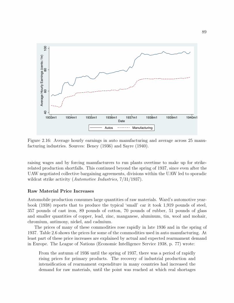
89

4060

8010

0Av

erag

e Ho

urly

Earn

ings

(cen

ts /

hr)

1933m1 1934m1 1935m1 1936m1 1937m1 1938m1 1939m1 1940m1Date

Autos Manufacturing

®

Figure 2.16: Average hourly earnings in auto manufacturing and average across 25 manu-facturing industries. Sources: Beney (1936) and Sayre (1940).

raising wages and by forcing manufacturers to run plants overtime to make up for strike-related production shortfalls. This continued beyond the spring of 1937, since even after theUAW negotiated collective bargaining agreements, divisions within the UAW led to sporadicwildcat strike activity (Automotive Industries, 7/31/1937).

Raw Material Price Increases

Automobile production consumes large quantities of raw materials. Ward’s automotive year-book (1938) reports that to produce the typical ‘small’ car it took 1,919 pounds of steel,357 pounds of cast iron, 89 pounds of cotton, 70 pounds of rubber, 51 pounds of glassand smaller quantities of copper, lead, zinc, manganese, aluminum, tin, wool and mohair,chromium, antimony, nickel, and cadmium.

The prices of many of these commodities rose rapidly in late 1936 and in the spring of1937. Table 2.6 shows the prices for some of the commodities used in auto manufacturing. Atleast part of these price increases are explained by actual and expected rearmament demandin Europe. The League of Nations (Economic Intelligence Service 1938, p. 77) wrote:

From the autumn of 1936 until the spring of 1937, there was a period of rapidlyrising prices for primary products. The recovery of industrial production andintensification of rearmament expenditure in many countries had increased thedemand for raw materials, until the point was reached at which real shortages

90

MaterialAverage 1936 Price

(cents / pound)

July 1937 Price

(cents / pound)

Percent

Change

Sheet steel 3.0 3.6 20.0%

Forging steel 1.6 1.9 16.8%

Cast iron 0.9 1.1 21.8%

Wool 88.1 98.0 11.2%

Rubber 16.5 19.0 15.2%

Copper 9.5 13.8 45.3%

Lead 4.7 6.0 27.7%

Zinc 5.3 7.3 37.7%

Table 2.6: Raw material prices. Source: Automotive Industries, 9/18/1937, p. 374.

of such materials were anticipated in spite of the relaxation of many restrictionschemes controlling their production and export. At this point, in view of thefear of future shortages, a speculative demand for commodities developed andwas superimposed upon the high normal demand.

The timing of the auto price increase

Manufacturers’ labor and raw material costs rose in spring 1937. However, auto prices werelittle changed until the introduction of new model year vehicles in the fall. The BLS wholesaleauto price index was literally unchanged from January to August 1937 (figure 2.14). Thisnominal rigidity distinguished the auto industry: in many other industries, costs rose in late1936 and early 1937. In these other industries, prices tended to rise at the same time ascosts rather than with a several month lag. Figure 2.17 shows the behavior of auto wholesaleprices along with those for processed food, home furnishing goods, and textiles. All pricesrise in late 1936 and / or early 1937. Auto prices are unique in rising further in fall 1937and remaining high during the recession.

Importantly, in the summer and early fall of 1937 contemporaries recognized that automanufacturers’ costs had risen and that this would lead to higher car prices in future months.For example, in an article published on July 31, 1937, the industry trade publication, Auto-motive Industries, reports (p. 135):

General Motors Corp. divisions had only ten days uninterrupted work from Feb.11, the date an agreement was signed with the United Automobile Workers,through the June quarter, stated Alfred P. Sloan, Jr., chairman of the board,bitterly assailing the union for its inability to prevent wildcat strikes. He blamedthe union for a decline in earnings during the second quarter compared with thelike quarter of 1936. He said the company was unable to meet the demand forits cars because of interference with production. Demand currently is equal to

91

6070

8090

100

110

Who

lesa

le p

rice

inde

xes,

n.s.

a., M

ay 1

937=

100

1933m1 1934m1 1935m1 1936m1 1937m1 1938m1 1939m1 1940m1Date

PPI AutosHouse furnishing goods Processed foodTextiles

®

Figure 2.17: Wholesale prices 1933-39. Sources: PPI - FRED series PPIACO; house fur-nishing goods - NBER macrohistory series m04095a; textiles - NBER macrohistory seriesm04064a; autos - NBER macrohistory series m04180b; processed foods - NBER macrohistoryseries m04055.

the company’s ability to supply. Indirectly, labor troubles had another effectupon earnings, Mr. Sloan pointed out. Net income declined in relation to unitand dollar sales volume as a result of two general wage increases, numerousadjustments, and the need for using high-cost night shift operations in an effort tomake up production deficiencies. Earnings were also affected by higher materialscosts. High car prices for 1938 will result, he forecasts.

Ford and General Motors, but not Chrysler, did raise prices some in August 1937, beforenew model year vehicles were introduced (Automotive Industries, 8/7/1937, 8/14/1937, and10/16/1937), but this price increase was seen as insufficient to cover the increase in costs thathad occurred (Automotive Industries 9/18/1937, p. 374). Hence further price increases wereexpected. The president of Buick told the press on September 13, 1937 (qtd. in AutomotiveIndustries 9/18/1937, p. 374): “We are not yet ready to disclose our price structure but Ican tell you that due to the increased cost of labor and materials the prices will have to besomewhat higher.”

92

2.5 How did the price shock impact sales?

Theory

Like an investment good, consumer durables purchases are likely to have a high intertem-poral elasticity of substitution (Barsky, House, and Kimball 2007). In particular, expectedfuture price increases will significantly increase current durables purchases as sales are pulledforward. The bulge in sales will be followed by a large drop in sales after the price increaseoccurs. Thus the elasticity of demand with respect to a price change that is expected will bemuch larger than the (static) elasticity of demand with respect to price. I shall argue thatthis phenomenon is the key to understanding how the price increase for 1938 model cars hadsignificant macroeconomic effects.

Narrative Evidence

As discussed above, during the summer and early fall of 1937 price increases were widely ex-pected within the auto industry. Contemporary industry observers reported that consumersalso expected prices to increase and that this drove up sales prior to the introduction of newmodel year vehicles in October and November. For example, an article on the front pageof the July 24, 1937 issue of Automotive Industries stated (p. 103): “The public has theimpression, probably well founded, that 1938 cars will be somewhat higher in price and notmuch different from the present models. This is leading to current buying in considerablevolume.” A confirmation of this view comes from an ad appearing in the San FranciscoChronicle on August 8 1937 (figure 2.18). This ad, for a Graham Supercharger, encouragescustomers to “buy now . . . before the price rise.” It suggests that higher prices wereexpected, and that they motivated purchases.

In 1938, General Motors sponsored a study on the impact of auto prices on demandwhich was presented at a joint meeting of the American Statistical Society and the Econo-metric Society in Detroit. The published volume begins with an essay by a General Motorsemployee S. L. Horner (1939) summarizing the reasons General Motors sponsored the studyand providing an overview of the determinants of auto demand. Horner emphasizes theimportance of price expectations, particularly in fall 1937 (p. 14-15):

During periods of rising costs, such as that which took place in 1937 when laborcosts were rising so rapidly, prospective automobile purchasers tend to anticipatean increase in the price of automobiles. This is particularly apt to be the casewhen the advance in costs continues over a considerable period of time without anincrease in automobile prices. Automobile buyers are sufficiently well informedto realize that any such increase in costs must, in time, cause an increase inautomobile prices. And, if they do not arrive at this conclusion themselves, theyare almost certain to have it impressed upon them by dealers and salesmen withinthe industry. Thus, during the spring and summer of 1937, dealers and salesmenwere urging people to buy their new cars, before prices increased. This tends to

93

Figure 2.18: From the San Francisco Chronicle, August 8 1937.

94

cause a bulge in sales which is followed, after prices are increased, by a declinein sales.

Horner attributes low sales in 1938 to the fact that “many people, anticipating that an in-crease in automobile prices would be made when the 1938 models were announced, purchasedcars in the 1937 model year which they otherwise would have purchased in 1938” (p. 14).

Quantitative evidence

The hypothesis that price expectations boosted sales in summer and early fall 1937 anddepressed sales in 1938 has a testable implication. If the hypothesis is true, then a statisticalmodel of auto sales that incorporates determinants of auto demand other than auto pricesand price expectations should underpredict sales in the summer of 1937 and overpredict salesin 1938. In this subsection, I construct such a model and use it to quantify the impact ofthe auto price shock.

In addition to autoregressive lags and seasonal dummies, there exist an almost limitlessnumber of possible variables that might have predictive power for auto sales. Even just 10possible right hand side variables, each with 12 possible lags means 1013 = 10, 000, 000, 000, 000possible models, far too many to consider. I proceed by considering only variables thatmeasure the stance of monetary and fiscal policy and / or were deemed important by con-temporary and current forecasters of auto sales.

Horner (1939) provides a useful guide to how contemporaries thought about the deter-minants of auto sales. He argues that the following equation fits annual sales well:

log(Sales)t = β0 + β1log(GNP )t + β2log(GNPt/GNPt−1) + εt (2.2)

As a guide to how modern economists forecast sales, I consider the reduced form forecast-ing equation for light vehicle sales in the Michigan model of the U.S. economy (Hymans et al.2002, equation C33). This equation includes two proxies for the state of the macroeconomy:a distributed lag of real personal disposable income and the change in the unemploymentrate.

Below I describe each variable I use and the reason for its inclusion.

Seasonal Effects

In the interwar period, auto sales exhibited a strong seasonal pattern, with winter sales farbelow summer sales. Seasonal patterns were partly driven by the weather: muddy roadsmade driving unpleasant or infeasible in much of the country during the winter and spring.But a large driver of seasonal patterns was also the introduction of new model vehicles. Until1935, new model vehicles were introduced in January of each year. Thereafter, in a changecoordinated through the National Industrial Recovery Act, new models were introduced inOctober or November (Cooper and Haltiwanger 1993). To account for the resulting changein seasonal patterns, I include both a full set of monthly dummies, and a set of monthlydummies interacted with a dummy variable equal to one in 1935 and after.

95

Real Personal Disposable Income

Both Horner (1939) and the Michigan model include a measure of national income. Horner(1939) uses GNP and the Michigan model uses real personal disposable income. For mypurposes, disposable income has the attractive feature that it both reflects the evolution ofwages and profits in the private sector and reflects changes in taxes and transfers. Thus itproxies for the state of the economy and fiscal policy actions. Unfortunately, there is nomonthly series for disposable income in the interwar period. But Harold Barger constructeda seasonally adjusted quarterly measure of nominal personal disposable income.29 I deflatethis by the CPI and convert it to a monthly series using a cubic spline.

Note that since auto sales cause income as well as vice versa, including real disposableincome in the forecasting model will bias the results against finding a large effect of theexogenous auto shock. For example, if sales were unusually low in 1938, this would havelowered real disposable income, leading my forecast to underestimate the level of sales thatwould have occurred absent the shock. Since I measure the impact of the shock as thedifference between forecast and actual sales, this would have the effect of reducing the sizeof the measured shock.

The Money Supply

Neither Horner (1939) nor the Michigan model include a measure of the money supply orinterest rates. However, since I wish to know what part of the decline in auto sales cannotbe accounted for by macro policy, I need a measure of monetary policy in the forecastingequation. Theory suggests that interest rates rather than the quantity of money ought tobe most directly linked to sales. The proportion of cars sold on credit exceeded 50 percentin every year from 1919-1939 (Olney 1999, Table II), providing an obvious channel throughwhich interest rates would be expected to impact sales. Since interest rates changed little in1937-38 (figure 2.2), however, they will be unable to forecast the decline in auto sales between1937 and 1938. To make sure I do not understate the possible impact of monetary policyon sales, I instead include the quantity of money, specifically the seasonally adjusted broadmoney stock (currency held by the public plus demand and time deposits of commercialbanks).30

Recession Dummy

The Michigan model includes the unemployment rate. Unfortunately this is unavailable ata monthly or quarterly frequency before 1929. As an indicator of general business cycleconditions, I instead incorporate a dummy variable equal to 1 in a month between an NBERbusiness cycle peak and trough (inclusive of the peak and trough month).

29NBER macrohistory series q08282a. Underlying source is “Unpublished data from the files of Dr. HaroldBarger.”

30NBER macrohistory series m14144a. Computed by the NBER from underlying data in Friedman andSchwartz (1970), Monetary Statistics of the United States.

96

Variable Lags considered

Log Auto Sales (Dependent variable) 1-12

Log Real Personal Disposable Income 0-12

Log Difference Money 0-12

Recession Dummy 0-12

Total number of specifications 26,364

Table 2.7: Lag possibilities for forecasting model

Lag selection

Ideally, one would like to consider all possible lag combinations of the above variables aswell as run the model with all variables in levels, logs, differences, and log differences. Tomake computational time reasonable, I limit these possibilities in several ways. First, Iconsider only models with the dependent variable (auto sales) in logs. Preliminary regressionssuggested this yielded as good a forecast (measured by information criteria) as any othertransformation of the dependent variable, and it is the form preferred by Horner (1939).Since there may be a trend to log auto sales, I include a time trend. Second, based on resultsfrom preliminary regressions, I include only the log of real personal disposable income, thelog difference of the money supply, and the level of the recession dummy. Third, I do notconsider specifications in which lags are skipped. Thus I consider, for example, all possiblespecifications with 4 lags or 12 lags of log disposable income, but I do not consider a modelwith just the 4th and the 12th lag. Table 2.7 summarizes the specifications I consider.

To choose what lags to include, one does not simply want to choose the model withthe best fit. Such a procedure would select an overparameterized model with poor out-of-sample performance. An approach to dealing with this problem is to select models byminimizing an information criterion. An information criterion rewards in-sample fit butpenalizes additional right hand side variables (or lags). For each model, I compute theAkaike information criterion (AIC) and Bayesian information criterion (BIC), where

AIC = Nln(SSR) + 2P, (2.3)

andBIC = Nln(SSR) + ln(N)P. (2.4)

N is the number of observations, SSR is the sum of squared residuals (computed relative tothe level of auto sales), and P is the number of parameters estimated (Enders 2004).

Both the AIC and BIC reward better fit and punish additional variables, but the BICpunishes additional variables more. The BIC will never select a model with more right handside variables than the model selected by the AIC. Both information criterion are standardand have theoretical appeal. Asymptotically, the BIC will select the correct model. But ina small sample, Monte Carlo studies suggest the AIC may perform better (Enders 2004). Ievaluate both the AIC and BIC for each possible specification.

97

Dependent variable is log auto sales

Lag log auto sales 0.694*** 0.539***

(0.0854) (0.0625)

Lag 2 lag auto sales -0.312***

(0.101)

Lag 3 log auto sales 0.151*

(0.0777)

Log real disposable income 1.100*** 1.066***

(0.248) (0.212)

Log difference money 2.214*** 2.489***

(0.708) (0.722)

Recession dummy 0.0392 0.0557

(0.0587) (0.0604)

Lag recession dummy -0.0896 -0.162**

(0.0806) (0.0626)

Lag 2 recession dummy -0.0620

(0.0619)

Time trend -0.00193*** -0.00194***

(0.000482) (0.000463)

Sample period

Observations 135 135

R-squared 0.969 0.965

AIC 1461 1463

BIC 1557 1551

*** p<0.01, ** p<0.05, * p<0.1

Preferred by

min. AIC

Preferred by

min. BIC

Jan. 1926-March 1937

Standard errors in parentheses

Table 2.8: Estimation results for specifications selected by AIC and BIC criteria. Seasonalterms and a constant are omitted from the table.

Results

Monthly auto sales data begins in 1925.31 To allow for up to 12 possible lags, I estimateeach model over the period January 1926-March 1937. I choose March 1937 as the enddate, since it is roughly when unionization was complete, and is thus the earliest consumerswould have started to expect price increases for the next model year. Table 2.8 shows theestimation results for the optimal specifications chosen by the AIC and BIC criterion. Bothspecifications are parsimonious and have excellent in-sample fit.

Figure 2.19 shows the predicted and actual path of auto sales in 1937 and 1938. Sincethe forecast is somewhat sensitive to the start date, I graph the AIC and BIC forecastsfor all start dates from January 1937-July 1937. The models perform poorly and disagree

31As is standard in the literature (e.g. Cooper and Haltiwanger 1993), I use new registrations as themeasure of sales. Unfortunately, data on actual sales are not reported in the interwar period. Purchasers ofnew cars were legally obligated to register their vehicles although some lag was possible (Survey of CurrentBusiness 1934). Data on registrations was reported monthly in the Survey of Current Business. I take thedata from NBER macrohistory series m01109.

98

1938 model introduction

Actual Sales

Forecast Sales

100

200

300

400

500

Sale

s, th

ousa

nds,

nsa

1937m1 1937m7 1938m1 1938m7 1939m1Date

®

Figure 2.19: Actual and forecast auto sales.

significantly in the spring of 1937, perhaps reflecting the effects of strikes in the auto andother industries.32 But beginning in mid-summer 1937, there is remarkable agreement amongthe forecast models. All predict sales below actual from July-November 1937, and all predictsales above actual from December 1937 to December 1938.

The forecast exercise fits - both quantitatively and qualitatively - remarkably well withthe narrative evidence and theoretical consumption response to an expected durable goodsprice increase. Up until the price increase occurs - in October and November 1937 - salesare higher than they otherwise would have been; after the price increase, sales are far lowerthan they would have been. One might ask why forecast sales are still below actual sales inNovember 1937? There are two possibilities: one is that 1937 model vehicles may still havebeen sold at the old lower price in the first part of the month. Second, since the sales dataare registrations, it may have some lag relative to actual sales.

Table 2.9 shows the quantitative implications of the forecasting exercise for the aggregateeconomy. Columns 1 and 2 show annual auto sales and forecast auto sales in 1936, 1937, and1938.33 If not for the price shock, unit sales would have fallen by ‘only’ 25 percent between1937 and 1938; instead, they fell by 46 percent. Columns 3 and 4 show the level and percent

32Automotive Industries, 7/31/37, p. 138 wrote: “Psychological unrest, combined with an actual lossof purchasing power due to the strikes in various industries this year, can probably be blamed more thananything else for the failure of automobile sales to set new records in May and June.”

33Forecast sales in 1937 equal actual sales through March plus forecast sales for April to December. Theforecast is the median of the specifications minimizing AIC and BIC for all start dates from January to July1937.

99

YearAuto sales

(thousands)

Auto sales w/o

auto price

shock

(thousands)

Real GDP

(1937 $s,

billions)

Change in real

GDP

Real GDP w/o

auto price

shock (1937

$s, billions)

Change in real

GDP w/o auto

price shock

1936 3404 87.4 13.1%

1937 3485 3309 91.9 5.1% 91.6 4.9%

1938 1890 2489 88.7 -3.5% 89.6 -2.3%

Table 2.9: Aggregate implications of forecasting exercise. Sources: Real GDP is from NIPAtable 1.1.6A. Auto sales data from NBER macrohistory series m01109 (see text).

change in real GDP. Column 5 shows counterfactual estimates of GDP without the autoprice shock. This is computed as

GDPcf = GDP + (Salescf − Sales) · P ·M, (2.5)

where Xcf is the counterfactual estimate of X, P is the average retail price of a passengervehicle, and M is the multiplier for automobile spending. For P , I use the estimate in Suits(1958, p. 279) for the average retail value of cars sold in 1937, $808. For the value of themultiplier, I use 1.8, the estimate of Gordon and Krenn (2010) for the government spendingmultiplier in 1940.34

The final column reports estimates of GDP growth without the auto shock. Expectationsof price increases boosted sales and thus GDP growth in 1937, but made the recession in1938 much more severe. The auto price shock explains over a third of the 1938 GDP decline.

2.6 Can the auto price shock explain the recession’s

anomalies?

Timing

Figure 2.20 shows the path of seasonally adjusted auto production and sales in 1937 and1938. As was generally true in the interwar period, production and sales are highly corre-lated (Cooper and Haltiwanger 1993). Auto manufacturers appeared to emphasize a target

34For more discussion of the likely size of the multiplier in conditions like those in 1937, see chapter 1,section 1.7.

My results scale linearly with the size of the multiplier. The table below shows the implications of twoalternative assumptions about the multiplier’s size.

Year Change in real GDP

Change in real GDP w/o auto price shock, M=1

Change in real GDP w/o auto price shock, M=2.5

1937 5.1% 5.0% 4.7%1938 -3.5% -2.8% -1.8%

100

Sales

Production10

020

030

040

0Th

ousa

nds,

sea

sona

lly a

djus

ted

1937m1 1937m7 1938m1 1938m7 1939m1Date

®

Figure 2.20: Seasonally adjusted auto sales and production. Sources: NSA data from NBERmacrohistory series m01109 and m01107a. Seasonally adjusted by regressing on monthlydummies and monthly dummies interacted with post 1935 dummy variable.

inventory level rather than production smoothing (Kashyap and Wilcox 1993). Thus as salescollapsed in fall 1937, so did production. To what extent does this decline explain the rapiddecline in industrial production as a whole?

Automobile production had a 4.79 percent weight in the Federal Reserve industrial pro-duction index (Federal Reserve Board 1940). Hence even very large swings in auto produc-tion can account only for modest swings in industrial production as a whole. The key tothe quantitative importance of auto production for movements in the IP index is the largeinput-output linkages between auto production and other manufacturing sectors. Fortu-nately, while working for the Bureau of Labor Statistics (BLS), Wassily Leontief constructeda 38x38 input-output table for the 1939 U.S. economy (BLS, undated). Although a smallerversion was published in Leontief (1951), until now the unpublished larger table appears tohave been unnoticed and unused by economists. The larger table is a valuable source ofinformation on the linkages connecting auto production with the rest of the economy.

Table 2.10 shows the share of net output consumed by the motor vehicle industry foreach Federal Reserve industry group. Demand from auto manufacturers was particularlyimportant for steel production. Aside from the construction sector, the auto industry wasthe largest purchaser of steel products. To get a rough quantitative sense of the importanceof the auto industry for the timing of IP movements, I construct an industrial productionindex that excludes autos and the share of other sectors consumed by the auto industry

101

Industry groupShare of net output purchased

by motor vehicles industry

Durable manufactures

Iron and steel 12.5%

Machinery 1.7%

Transportation equipment ex. autos 0.0%

Nonferrous metals and their products 5.2%

Lumber and products 0.7%

Stone, clay, and glass Products 2.7%

Nondurable manufactures

Textiles and products 0.9%

Leather and products 0.4%

Manufactured food products 0.0%

Alcoholic beverages 0.0%

Tobacco products 0.0%

Paper and products 0.1%

Printing and publishing 0.0%

Petroleum and coal products 0.4%

Chemicals 0.9%

Rubber products 19.8%

Minerals

Fuels 0.4%

Metals 10.6%

Table 2.10: Share of industry group output purchased by the motor vehicle industry. Cal-culated from 1939 38x38 input-output in BLS (undated).

(‘purged IP’). Formally,

IPxauto,t = IPt − vautoIPauto,t −18∑i=1

wiviIPi,t, (2.6)

where wi is the share of industry group i net output purchased by the auto industry, vi is theshare of industry group i in total industrial production, and IPi,t is the seasonally adjustedvalue of the industrial production index for industry group i (indexed to 1935-39=100).Industrial output weights and indexes are from the Federal Reserve (1940).

Figure 2.21 shows the path of total and purged industrial production in 1937 and 1938.In the summer of 1937, when auto sales are brought forward due to expected higher prices,total industrial production (which includes autos) exceeds the purged index. This resultconfirms the view expressed in the The Review of Economics and Statistics summary of the1937 economy that “During the spring and summer months [of 1937], the maintenance ofmanufacturing output at the high level attained in 1936 was due almost entirely to sustainedactivity in the iron and steel and automobile industries” (Crum, Gordon, and Wescott 1938,p. 45). In the late fall, once auto prices rise, total IP falls below purged IP. This exercisesuggests that the auto shock likely contributed to the very rapid decline of industrial pro-

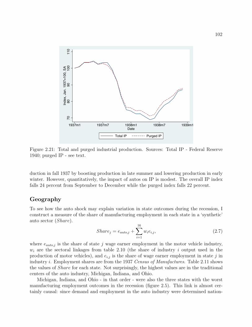
102

70

80

90

10

01

10

Ind

ex,

Ja

n.

19

37

=1

00

, S

A

1937m1 1937m7 1938m1 1938m7 1939m1Date

Total IP Purged IP

®

Figure 2.21: Total and purged industrial production. Sources: Total IP - Federal Reserve1940; purged IP - see text.

duction in fall 1937 by boosting production in late summer and lowering production in earlywinter. However, quantitatively, the impact of autos on IP is modest. The overall IP indexfalls 24 percent from September to December while the purged index falls 22 percent.

Geography

To see how the auto shock may explain variation in state outcomes during the recession, Iconstruct a measure of the share of manufacturing employment in each state in a ‘synthetic’auto sector (Share).

Sharej = eauto,j +16∑i=1

wiei,j, (2.7)

where eauto,j is the share of state j wage earner employment in the motor vehicle industry,wi are the sectoral linkages from table 2.10 (the share of industry i output used in theproduction of motor vehicles), and ei,j is the share of wage earner employment in state j inindustry i. Employment shares are from the 1937 Census of Manufactures. Table 2.11 showsthe values of Share for each state. Not surprisingly, the highest values are in the traditionalcenters of the auto industry, Michigan, Indiana, and Ohio.

Michigan, Indiana, and Ohio - in that order - were also the three states with the worstmanufacturing employment outcomes in the recession (figure 2.5). This link is almost cer-tainly causal: since demand and employment in the auto industry were determined nation-

103

State Share State Share

AL 4.6% NE 0.6%

AZ 2.4% NV 0.1%

AR 0.7% NH 0.7%

CA 4.7% NJ 5.3%

CO 3.0% NM 0.5%

CT 4.8% NY 4.1%

DE 4.0% NC 0.9%

FL 1.9% ND 0.1%

GA 1.4% OH 9.8%

ID 0.5% OK 1.7%

IL 4.0% OR 1.6%

IN 10.4% PA 5.5%

IA 1.8% RI 2.5%

KS 1.6% SC 0.9%

KY 2.2% SD 0.2%

LA 2.7% TN 1.8%

ME 3.4% TX 2.9%

MD 7.1% UT 1.0%

MA 3.2% VT 1.2%

MI 29.7% VA 6.5%

MN 2.7% WA 2.5%

MS 0.7% WV 3.8%

MO 3.5% WI 8.0%

MT 0.3% WY 0.3%

Table 2.11: Share of employment in each state in the synthetic auto sector. Sources: Seetext.

wide, it cannot have been poor conditions in these states that caused the decline in autoindustry employment. And it is unclear what, if any, third factor would have caused bothan outsized decline in auto industry employment and poor employment in outcomes in thesethree states.

There is some evidence that contemporaries noticed this link and blamed the auto indus-try. A.A. Berle Jr., the assistant secretary of state, advocated government planning of autoproduction noting that “the motor industry in 1937 undertook largely to increase its outputand sales. It did this at the cost of suspending much of its activities in 1938 and causingwidespread distress in the Detroit and Ohio areas” (Automotive Industries, 8/27/1938, p.242). General Motors in particular attracted public attention when on one day, January 11938, it laid off 30,000 workers (Automotive Industries, 1/1/38 and 1/15/38).

To more formally assess the link between the auto sector and state employment outcomes,I estimate the simple regression of state employment change on Share. Results are in ta-ble 2.12. Panel A includes Michigan while panel B excludes Michigan. Not surprisingly, thehigh share of employment linked to the auto industry explains why Michigan does so poorlyin the recession, and hence excluding Michigan from the regression reduces the statisticalsignificance of Share and the R2. The tables also shows results for subsets of states with

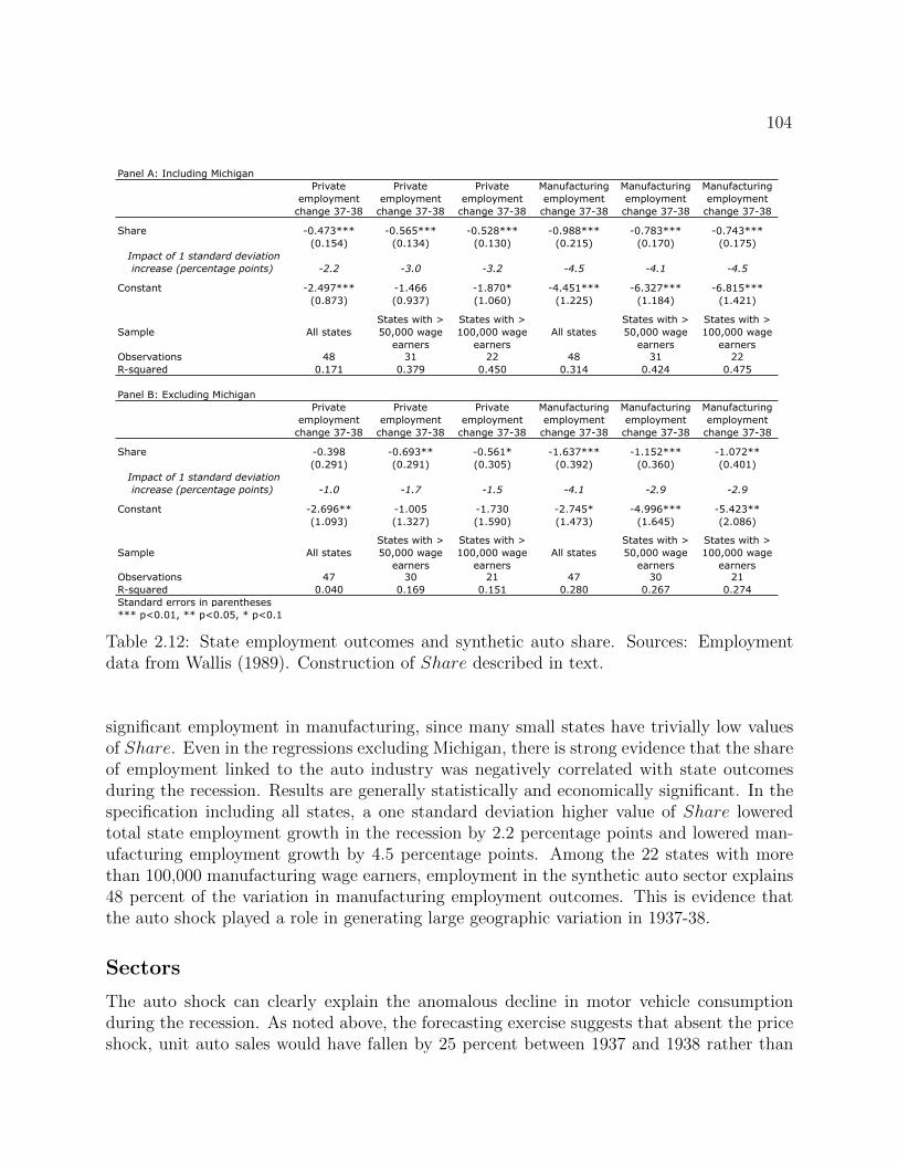
104

Panel A: Including Michigan

Private

employment

change 37-38

Private

employment

change 37-38

Private

employment

change 37-38

Manufacturing

employment

change 37-38

Manufacturing

employment

change 37-38

Manufacturing

employment

change 37-38

Share -0.473*** -0.565*** -0.528*** -0.988*** -0.783*** -0.743***

(0.154) (0.134) (0.130) (0.215) (0.170) (0.175)

Impact of 1 standard deviation

increase (percentage points) -2.2 -3.0 -3.2 -4.5 -4.1 -4.5

Constant -2.497*** -1.466 -1.870* -4.451*** -6.327*** -6.815***

(0.873) (0.937) (1.060) (1.225) (1.184) (1.421)

Sample All states

States with >

50,000 wage

earners

States with >

100,000 wage

earners

All states

States with >

50,000 wage

earners

States with >

100,000 wage

earners

Observations 48 31 22 48 31 22

R-squared 0.171 0.379 0.450 0.314 0.424 0.475

Panel B: Excluding Michigan

Private

employment

change 37-38

Private

employment

change 37-38

Private

employment

change 37-38

Manufacturing

employment

change 37-38

Manufacturing

employment

change 37-38

Manufacturing

employment

change 37-38

Share -0.398 -0.693** -0.561* -1.637*** -1.152*** -1.072**

(0.291) (0.291) (0.305) (0.392) (0.360) (0.401)

Impact of 1 standard deviation

increase (percentage points) -1.0 -1.7 -1.5 -4.1 -2.9 -2.9

Constant -2.696** -1.005 -1.730 -2.745* -4.996*** -5.423**

(1.093) (1.327) (1.590) (1.473) (1.645) (2.086)

Sample All states

States with >

50,000 wage

earners

States with >

100,000 wage

earners

All states

States with >

50,000 wage

earners

States with >

100,000 wage

earnersObservations 47 30 21 47 30 21

R-squared 0.040 0.169 0.151 0.280 0.267 0.274

Standard errors in parentheses

*** p<0.01, ** p<0.05, * p<0.1

Table 2.12: State employment outcomes and synthetic auto share. Sources: Employmentdata from Wallis (1989). Construction of Share described in text.

significant employment in manufacturing, since many small states have trivially low valuesof Share. Even in the regressions excluding Michigan, there is strong evidence that the shareof employment linked to the auto industry was negatively correlated with state outcomesduring the recession. Results are generally statistically and economically significant. In thespecification including all states, a one standard deviation higher value of Share loweredtotal state employment growth in the recession by 2.2 percentage points and lowered man-ufacturing employment growth by 4.5 percentage points. Among the 22 states with morethan 100,000 manufacturing wage earners, employment in the synthetic auto sector explains48 percent of the variation in manufacturing employment outcomes. This is evidence thatthe auto shock played a role in generating large geographic variation in 1937-38.

Sectors

The auto shock can clearly explain the anomalous decline in motor vehicle consumptionduring the recession. As noted above, the forecasting exercise suggests that absent the priceshock, unit auto sales would have fallen by 25 percent between 1937 and 1938 rather than

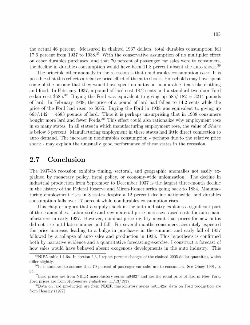
105

the actual 46 percent. Measured in chained 1937 dollars, total durables consumption fell17.6 percent from 1937 to 1938.35 With the conservative assumption of no multiplier effecton other durables purchases, and that 70 percent of passenger car sales were to consumers,the decline in durables consumption would have been 11.8 percent absent the auto shock.36

The principle other anomaly in the recession is that nondurables consumption rises. It ispossible that this reflects a relative price effect of the auto shock. Households may have spentsome of the income that they would have spent on autos on nondurable items like clothingand food. In February 1937, a pound of lard cost 18.2 cents and a standard two-door Fordsedan cost $585.37 Buying the Ford was equivalent to giving up 585/.182 = 3214 poundsof lard. In February 1938, the price of a pound of lard had fallen to 14.2 cents while theprice of the Ford had risen to $665. Buying the Ford in 1938 was equivalent to giving up665/.142 = 4683 pounds of lard. Thus it is perhaps unsurprising that in 1938 consumersbought more lard and fewer Fords.38 This effect could also rationalize why employment rosein so many states. In all states in which manufacturing employment rose, the value of Shareis below 3 percent. Manufacturing employment in these states had little direct connection toauto demand. The increase in nondurables consumption - perhaps due to the relative priceshock - may explain the unusually good performance of these states in the recession.

2.7 Conclusion

The 1937-38 recession exhibits timing, sectoral, and geographic anomalies not easily ex-plained by monetary policy, fiscal policy, or economy-wide unionization. The decline inindustrial production from September to December 1937 is the largest three-month declinein the history of the Federal Reserve and Miron-Romer series going back to 1884. Manufac-turing employment rises in 8 states despite a 12 percent decline nationwide, and durablesconsumption falls over 17 percent while nondurables consumption rises.

This chapter argues that a supply shock in the auto industry explains a significant partof these anomalies. Labor strife and raw material price increases raised costs for auto man-ufacturers in early 1937. However, nominal price rigidity meant that prices for new autosdid not rise until late summer and fall. For several months consumers accurately expectedthe price increase, leading to a bulge in purchases in the summer and early fall of 1937followed by a collapse of auto sales and production in 1938. This hypothesis is confirmedboth by narrative evidence and a quantitative forecasting exercise. I construct a forecast ofhow sales would have behaved absent exogenous developments in the auto industry. This

35NIPA table 1.1.6a. In section 2.3, I report percent changes of the chained 2005 dollar quantities, whichdiffer slightly.

36It is standard to assume that 70 percent of passenger car sales are to consumers. See Olney 1991, p.95.

37Lard prices are from NBER macrohistory series m04027 and are the retail price of lard in New York.Ford prices are from Automotive Industries, 11/13/1937.

38Data on lard production are from NBER macrohistory series m01142a; data on Ford production arefrom Heasley (1977).

106

exercise implies that in 1938, 600,000 more cars would have been sold, and GDP growthwould have been 1.2 percentage points higher. Equally important, there is strong evidencethat the auto shock contributed to the anomalous timing, geographic, and sectoral patternsof output in the recession. Absent this shock, the 1937-38 recession would have been bothless severe and less unusual.

107

Table A.1: Quarterly output data

GDP Peak-TroughChange in

real GDP

Change in

durables

consump.

Change in

non-

durables

consump.

Change in

equipment

and

software

investment

Change in

nonresidential

structures

investment

Change in

residential

investment

1920:3-1921:4 -3.4% -14.5% 6.2% -41.1% 84.0% -12.6%

1923:4-1924:2 -0.5% -5.5% 1.4% -9.2% 2.6% -4.1%

1926:3-1927:3 -1.3% -5.8% 0.2% -11.5% -10.9% 0.3%

1929:1-1932:4 -32.7% -51.0% -17.2% -72.4% -72.9% -78.9%

1937:2-1938:2 -6.6% -24.2% 1.3% -38.1% -32.3% -25.4%

1948:4-1949:4 -1.6% 16.2% 1.4% -16.5% -14.5% 10.8%

1953:2-1954:1 -2.6% -6.4% 0.2% -5.3% -2.0% -3.6%

1957:3-1958:1 -3.7% -7.7% -1.5% -14.2% -9.6% -4.1%

1960:1-1960:4 -1.6% -1.1% 0.6% -5.8% -1.5% -11.1%

1969:3-1970:1 -0.6% -1.9% 1.5% -1.0% -1.2% -7.1%

1973:4-1975:1 -3.2% -8.7% -3.4% -9.5% -10.1% -30.2%

1980:1-1980:3 -2.2% -6.8% -1.6% -5.9% -4.4% -17.1%

1981:3-1982:1 -2.9% -4.2% 0.6% -2.7% 0.0% -15.4%

1990:2-1991:1 -1.4% -6.4% -0.8% -2.3% -3.8% -16.2%

2007:4-2009:2 -5.1% -13.3% -3.7% -22.1% -21.0% -36.1%

Note: Excludes the post World War II recession. The 2001 recession is also excluded sinceGDP barely declines. Sources: Gordon and Krenn (2010) for interwar recessions; thereafterNIPA table 1.1.3.

A Appendix

108

Chapter 3

Growth After a Financial Crisis: TheU.S. in Spring 1933

3.1 Introduction

From its low point in March 1933, seasonally adjusted industrial production rose 57 per-cent in four months.1 The speed of the recovery is surprising given Reinhart and Rogoff’s(2009, 2010) argument that recoveries after financial crises are usually slow.2 Yet after thenearly complete collapse of the banking system in March 1933, the U.S. experienced its mostrapid four months of growth since at least World War I. The existing literature has em-phasized two explanations for the economy’s emergence from the Depression in spring 1933.Eggertsson (2008) argues that Franklin Roosevelt’s words and fiscal actions raised inflationexpectations thus lowering real interest rates and stimulating consumption and investment.Temin and Wigmore (1990) also argue that inflation expectations mattered, but in additionstress the importance of the direct effect on farmers of the U.S. abandonment of the goldstandard. They argue that devaluation raised crop prices, thus increasing farm income andconsumption.

It has been difficult to disentangle a distinct farm channel from the overall expecta-tions channel absent high frequency geographically disaggregated data. We have not knownwhether recovery proceeded more or less rapidly in North Dakota or in New York. Butknowledge of the sources of recovery in spring 1933 is critically important and not only forour understanding of the end of the Depression. Spring 1933 is an analogy for policymakerstoday. Then, like now, interest rates were at the zero lower bound, and the economy hadsuffered a deep, financial-crisis induced recession. Did the economy start to recover because

1FRED series INDPRO.2Reinhart and Rogoff argue that the Great Depression experience fits with their story. They date the

financial crisis associated with the Great Depression to 1929 and hence include the Depression itself in theircalculations of growth after the crisis. One obtains quite different results if one dates the financial crisis to1933 instead. Regardless, rapid growth beginning in 1933 poses a puzzle for the view that a financial crisisdooms an economy to a slow recovery.

109

Franklin Roosevelt’s leadership changed inflation expectations? Or did it recover becauseof the direct effects of dollar devaluation on farm income? The answer has implications forcontemporary macropolicy. For instance, as of this writing, Japan is attempting a monetarypolicy regime shift, in part modeled on Roosevelt’s actions (Aso 2013). A better under-standing of spring 1933 may inform economists’ predictions about current Japanese policy(Romer 2013).

This is not to imply that Japan’s situation is exactly analogous to that of the U.S. inspring 1933. Among many other differences, Japan is a far more open economy now than theU.S. was in 1933. Total trade (exports plus imports) were 7.4 percent of U.S. GDP in 1933,3

whereas total trade is 29.8 percent of GDP in Japan today.4 The small share of trade in theU.S. meant that departure from the gold standard in 1933 could not contribute significantlyto growth by raising exports and reducing imports. And in fact, the trade deficit widened in1933 (NIPA table 1.1.6).5 By contrast, trade is a large enough share of Japanese GDP todaythat depreciation of the yen may well boost growth through this conventional channel. Butwhile trade is more important for Japan now than for the U.S. in 1933, agriculture is far lessimportant. In 1930, the farm share of the population in the U.S. was 25 percent,6 in Japantoday it is 5 percent.7 Thus the farm income channel that is in part the focus of this paperis unlikely to be significant in Japan today.

The contribution of this paper is to provide the data needed to test whether there wasa direct channel, distinct from general expectation effects, on U.S. recovery through agricul-ture in 1933. If, as Eggertsson (2008) argues, recovery was due to economy-wide inflationexpectations with no distinct role for farmers, then the increase in consumption demandought to have been relatively uniform across states. If, by contrast, production was spurredby demand from farmers, then consumer demand ought to have risen more rapidly in stateswith larger rural population shares. I exploit a previously unused dataset of monthly, statelevel auto sales to see whether the share of a state population’s engaged in farming was cor-related with auto sales recovery in spring 1933. I find that it was. A one standard deviationincrease in the share of a state’s population living on farms was associated with roughly a25 percentage point increase in auto sales growth from late winter to early summer 1933.In aggregate, my results imply that the recovery, at least as measured by auto sales, mighthave been as much as 50 percent slower if farm demand had not grown more rapidly thandemand in the economy as a whole. This suggests that recovery was not simply due to auniform change in inflation expectations but also to some factor that differentially benefitedfarmers. An explanation of recovery in spring 1933 should account for this fact.

This paper relates most obviously to the literature on U.S. recovery after 1933. Most

3NIPA table 1.1.64FRED series JPNEXPORTQDSNAQ, JPNIMPORTQDSNAQ, JPNRGDPQDSNAQ.5Eichengreen (1992, pp. 343-344) argues that this is explained by expectations of further dollar depre-

ciation; exporters had an incentive to wait to sell goods until the dollar was weaker.6Data are from the IPUMS 5% sample from the 1930 Census (Ruggles et al. 2010).7http://www.ers.usda.gov/topics/international-markets-trade/countries-regions/japan/

basic-information.aspx#.UZG6-ysjo9s.

110

of this work (e.g. Romer 1992, Cole and Ohanian 2004) does not focus on the economy’sturn-around in March and the initial spurt of growth thereafter. Prominent exceptions areTemin and Wigmore (1990) and Eggertsson (2008). Both argue that the key to growth was aregime change. In particular, by taking the U.S. off the gold standard and explicitly voicinghis desire for higher prices, both papers credit Roosevelt with inducing inflation expectations.The argument is that higher expected inflation lowered real interest rates, thus stimulatingdemand for investment goods and consumer durables.8 9 At the same time, Eggertsson andTemin and Wigmore stress that Roosevelt’s actions also led to expectations of higher futureoutput. Consumers and businesses expecting better times in the future were more willing tospend.10

While both Temin and Wigmore and Eggertsson emphasize the effect of higher inflationexpectations, their interpretation of the source of higher expected inflation is somewhatdifferent. Temin and Wigmore highlight Roosevelt’s decision to take the U.S. off the goldstandard, arguing that this was the key signal that prices would rise. Eggertsson doesnot disagree that departure from the gold standard was a necessary condition for recovery,but he focuses more on Roosevelt’s fiscal actions. He suggests that larger deficits gave thegovernment an incentive to inflate away nominal debt, thus making higher future inflationcredible.

In keeping with their focus on the effect of dollar devaluation, Temin and Wigmore arguethat a weaker dollar not only led to higher expected inflation, but also was expansionarythrough its effect on current and expected farm incomes. In their words (p. 495):

“Grain and cotton prices rose as the value of the dollar fell. Farmers and therural community looked forward to higher incomes as the higher prices for bothproduction and inventories worked through the rural community. These peoplestepped up their purchases of durables accordingly, of which the most importantwas automobiles. This encouraged a rise in auto production, steel production,and industrial production in general.”

Temin and Wigmore provide circumstantial evidence for this view. But absent monthlydata on state auto sales, they are unable to show that farmers bought more durables thannon-farmers in spring 1933.11 This paper fills this gap. It confirms Temin and Wigmore’shypothesis that auto sales grew more rapidly in more rural states. However, I argue that

8Romer (1992) argues that a similar channel led to growth between 1933 and 1940.9Eichengreen (1992) emphasizes not the rapidity of the 1933 recovery but its incompleteness. After

rising 57 percent from March to July, seasonally adjusted industrial production fell 19 percent from Julyto November, before rising again (FRED series INDPRO). Despite this, March 1933 was a decisive break:before, the trend had been steadily downward, thereafter upward. While the unevenness of the recoveryin 1933 is of obvious interest, the focus of this paper is narrower: what caused the initial turn-around andgrowth spurt in spring 1933?

10In the context of a continuous time New Keynesian model, Werning (2012) shows the importance ofhigher expected future output in a liquidity trap.

11Temin and Wigmore’s principal evidence comes from a state-level regression of the level of auto salesin all of 1933 on farm income and other income in 1933. They interpret a larger coefficient on farm income

111

this fact is consistent with a number of explanations of the recovery, not only a farm incomechannel through crop prices. Firmly establishing why auto sales grew so much more rapidly inrural states is beyond the scope of this paper. But I consider the implications and evidencefor two possible explanations: Temin and Wigmore’s farm income channel and a channelthrough farm debt and rural bank health.

At one extreme, consider a channel from devaluation to income through relative pricechanges. In the short run, devaluation increased crop prices but had little effect on theoverall price level. Thus the relative price of farm products rose. Farmers were better off. Atthe same time, consumers of farm products, whether urban workers or manufacturing firms,were worse off. As rural consumption rose, urban consumption ought to have declined. Inorder to break this symmetry, one must argue that there was some factor that made thepositive effect of higher crop prices on farmers larger than the negative effect of higher cropprices on urban workers. One such factor may have been inflation expectations. I suggestthat higher crop prices directly raised inflation expectations, so that the depressing effecton urban consumption from lower incomes was balanced by a stimulus to consumption fromexpected price increases.

While understanding the economy’s behavior in spring 1933 is itself important, thischapter is also relevant to the growing literature on the role of macro policy at the zero lowerbound. In the U.S. in spring 1933, as in Japan since the mid-1990s, and much of the developedworld since 2008, short-term interest rates were near zero, and hence conventional monetarypolicy was ineffective. Economists continue to debate the extent to which unconventionalmonetary policy can stimulate an economy in these conditions.12 This chapter adds to thisliterature by providing evidence on how policy led to rapid growth in 1933.

The next section revisits the aggregate data and documents the sectoral compositionof the recovery in spring 1933. Section 3.3 uses monthly data on state auto sales to showthat recovery proceeded more rapidly in agricultural states. Section 3.4 considers possibleimplications of these quantitative results. Section 3.5 concludes and suggests directions forfuture research.

3.2 Aggregate data

Before turning to explanations of the economy’s growth in the spring of 1933, it is useful toreexamine the data. Given that the period of especially rapid growth is just four months,from March to July 1933, it is natural to ask how sensitive our measurement of growth

as evidence in support of their hypothesis. While suggestive, this regression has two limitations: first, theleft-hand side variable is the level of auto sales, while their hypothesis is about the growth of auto sales.Second, the regression uses annual data, hence it conflates auto sales in the period of interest, spring 1933,with sales later in the year.

12The existence of the liquidity trap (i.e. the zero lower bound on interest rates) and its implications formonetary policy was first described by Keynes (1936) and Hicks (1937). Interest was reignited after ratesfell to near zero in Japan in the mid-1990s (Krugman 1998). Svensson (2003) and Woodford (2012) provideuseful overviews.

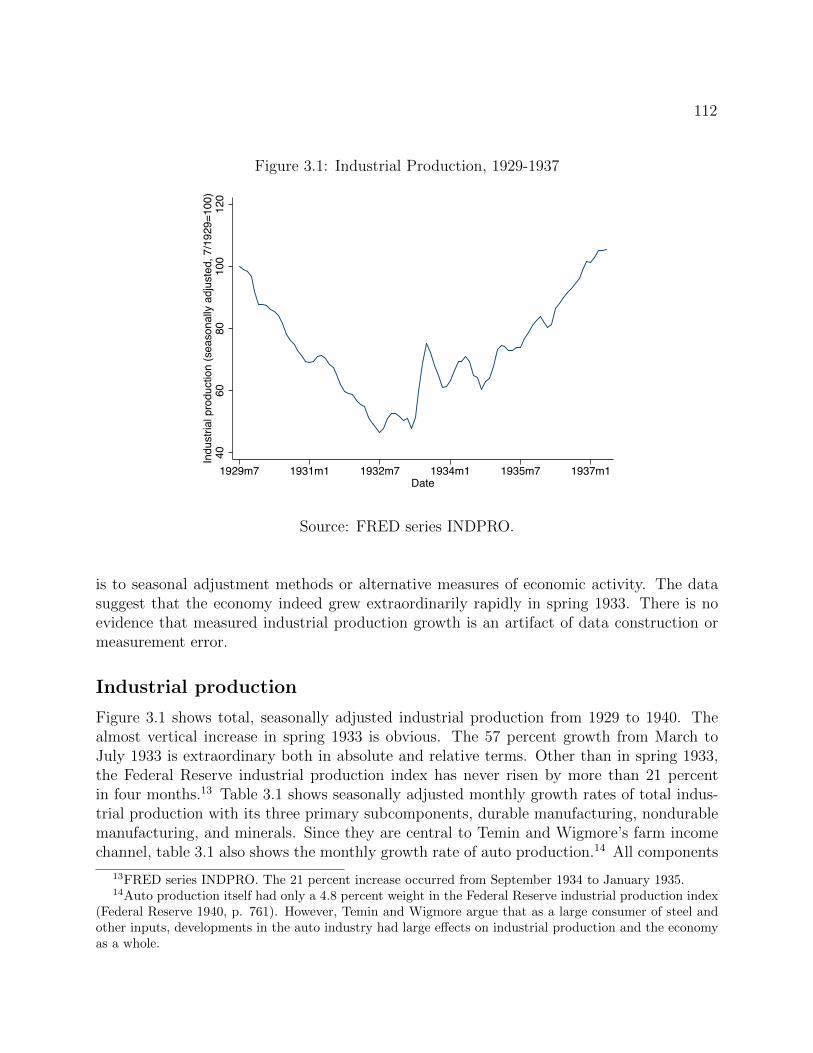
112

Figure 3.1: Industrial Production, 1929-1937

4060

8010

012

0In

dust

rial p

rodu

ctio

n (s

easo

nally

adj

uste

d, 7

/192

9=10

0)

1929m7 1931m1 1932m7 1934m1 1935m7 1937m1Date

Source: FRED series INDPRO.

is to seasonal adjustment methods or alternative measures of economic activity. The datasuggest that the economy indeed grew extraordinarily rapidly in spring 1933. There is noevidence that measured industrial production growth is an artifact of data construction ormeasurement error.

Industrial production

Figure 3.1 shows total, seasonally adjusted industrial production from 1929 to 1940. Thealmost vertical increase in spring 1933 is obvious. The 57 percent growth from March toJuly 1933 is extraordinary both in absolute and relative terms. Other than in spring 1933,the Federal Reserve industrial production index has never risen by more than 21 percentin four months.13 Table 3.1 shows seasonally adjusted monthly growth rates of total indus-trial production with its three primary subcomponents, durable manufacturing, nondurablemanufacturing, and minerals. Since they are central to Temin and Wigmore’s farm incomechannel, table 3.1 also shows the monthly growth rate of auto production.14 All components

13FRED series INDPRO. The 21 percent increase occurred from September 1934 to January 1935.14Auto production itself had only a 4.8 percent weight in the Federal Reserve industrial production index

(Federal Reserve 1940, p. 761). However, Temin and Wigmore argue that as a large consumer of steel andother inputs, developments in the auto industry had large effects on industrial production and the economyas a whole.

113

of industrial production rose from March to July 1933, but the most dramatic increase wasin durable manufacturing, with auto production rising even more rapidly than durable man-ufacturing as a whole. In the four-month period, seasonally adjusted durable manufacturinggrew 138 percent and autos production 152 percent, while nondurable manufacturing rose42 percent and mining 17 percent.

Table 3.1: Industrial production, monthly growth rates in 1933 (%)

Month Total IP Dur. Manu. Autos Nondur. Manu. Minerals

January 0.0 0.0 25.7 0.0 1.5February -1.7 -5.1 -25.0 -1.4 4.5March -5.3 -13.5 -18.2 -5.7 4.3April 7.4 21.9 51.9 9.1 -9.7May 17.2 25.6 19.5 13.9 15.4June 14.7 28.6 20.4 11.0 5.3July 10.3 20.6 15.3 3.3 6.3August -4.7 -3.9 5.9 -6.4 3.6September -6.1 -8.2 2.8 -4.5 -5.7October -5.2 -4.5 -2.7 -4.8 -7.3November -5.5 -15.6 -51.4 -2.5 1.3December 1.4 5.6 2.9 0.0 -1.3

Note: All series were seasonally adjusted by the Federal Reserve (1940).Source: Data are from Federal Reserve (1940).

The other striking feature of the table is the decline in industrial production after July.From July to November 1933 total industrial production fell 19 percent. This partial reversalof the spring recovery is apparent in all the major components of industrial production. Autoproduction also fell back, with an extraordinarily bad month in November 1933. While thischapter’s focus is on the initial burst of growth in spring 1933, an explanation for this growthought also to provide a clue as to why production fell in fall 1933.

Such rapid growth rates over a short period naturally lead to questions of data quality:should one believe that seasonally adjusted industrial production rose 57 percent in spring1933 or might this increase be a figment of data construction problems? The data suggestthe former. The first check is to consider the behavior of non-seasonally adjusted production.This is shown in figure 3.2. The rapid increase in industrial production is also present in theraw, non-seasonally adjusted data and is not a regular seasonal phenomena. Only in 1933does one see such a dramatic increase in spring.

114

Figure 3.2: Non-seasonally adjusted and seasonally adjusted industrial production

4050

6070

80In

dust

rial p

rodu

ctio

n (7

/192

9=10

0)

1931m1 1932m1 1933m1 1934m1 1935m1Date

NSA SA

Source: Federal Reserve Board, G.17 data release.

Other production indicators

A second check is to consider alternative seasonally adjusted indicators of economic activity.Figure 3.3 shows two such indicators: the Federal Reserve index of freight car loadingsand nonagricultural employment (Federal Reserve, 1941). Freight car loadings measure thereal quantity of shipments by rail in the period, with underlying data from the railroadsthemselves. The broad picture is similar to that for industrial production. After reachinga trough in March 1933, seasonally adjusted freight car loadings grew rapidly through July.In these four months, the seasonally adjusted series rose 40 percent.

It is also natural to examine the evolution of employment. Caution is necessary since theemployment data are not entirely independent of the industrial production data. For someindustries, the industrial production figures rely heavily on the Bureau of Labor Statisticsestablishment survey, which is the employment data’s source (Federal Reserve, 1940, p. 761).Nonetheless, it is reassuring that, like industrial production, employment rose rapidly inspring 1933. Total, seasonally adjusted, nonagricultural employment grew from 26.7 millionin March 1933 to 28.4 million in July.15 Seventy-three percent of this employment increasewas accounted for by an astonishing 20 percent increase in manufacturing employment.16

15Note that these employment data exclude relief workers. Data are from Federal Reserve (1941) p. 534.16Manufacturing employment rose from 6.12 million in March to 7.36 million in July (Federal Reserve,

1941, p. 534).

115

Figure 3.3: Freight car loadings and employment

27,0

0028

,000

29,0

0030

,000

31,0

0032

,000

SA, T

hous

ands

4050

6070

80SA

, Ind

ex 7

/192

9=10

0

1931m1 1932m1 1933m1 1934m1 1935m1Date

Freight car loadings Nonag. employment (right axis)

Source: Federal Reserve (1941).

Sales

Together, the data on industrial production, employment, and freight car loadings leave littledoubt that output rose rapidly in spring 1933. But was the recovery of production due tocontemporaneous consumer demand or to expectations of future demand? If the former,the historians’ task is to explain the increase in consumption. If the latter, to explain whyfirms expected higher future sales. Therefore I examine the behavior of sales in spring1933. Figure 3.4 shows seasonally adjusted passenger car sales and production from 1931through 1934.17 Seasonally adjusted sales behave similarly to production in spring 1933,roughly doubling from March to July. Figure 3.5 presents the analogous data for trucks.Interestingly, the recovery of truck sales is even more rapid than that of car sales in spring

17Sales data are from NBER macrohistory series m01109; production data are from NBER series m01107a.Neither series was seasonally adjusted by the source. I seasonally adjust the series by regressing the naturallogarithm of each series on monthly dummies and monthly dummies interacted with a post 1935 dummyvariable. The second set of dummies are necessary since the date of new model introduction - an importantdeterminant of car sales and production - changed in 1935 (Cooper and Haltiwanger 1993). The sampleperiod for the regression is January 1925 to December 1940. The series graphed in figure 3.4 is eεt · yx , whereεt are the residuals from the regression of the natural log of sales or production on the monthly dummies, yis the mean of non-seasonally adjusted sales over the period, and x is the mean of eεt .

116

Figure 3.4: Seasonally adjusted car sales and production

5010

015

020

025

0SA

, tho

usan

ds o

f uni

ts)

1931m1 1932m1 1933m1 1934m1 1935m1Date

Car sales Car production

Note: See text for details on the seasonal adjustment. Note that production data are mea-sured in actual units produced and hence differ slightly from the index of auto productionproduced by the Federal Reserve as part of its industrial production index. Thus the produc-tion data graphed here are similar but not identical to the auto production figures reportedin table 3.1.Source: Sales data are from NBER macrohistory series m01109; production data are fromNBER series m01107a.

1933: they rise 163 percent from March to July.18 Unfortunately, the more rapid growth oftruck sales does little to distinguish between the overall inflation expectations channel anda farm specific channel. It is consistent both with high demand for trucks from businessesand from farmers.

As with cars, the difference between truck production and sales is not obviously anoma-lous in spring 1933. Figures 3.4 and 3.5 suggest a roughly parallel movement in productionand sales in the motor vehicles sector. Thus explanations of the recovery, at least of thisimportant sector, must explain a rise not only in production, but also in consumer andinvestment demand.19

Department store sales provide another measure of consumer demand. Figure 3.6 showsthe behavior of seasonally adjusted department store sales.20 They show a rather different

18Sales data are from NBER macrohistory series m01146a; production data are from NBER seriesm01144a. The seasonal adjustment procedure is identical to that for passenger cars. See footnote above.

19This casts doubt on Kindleberger’s (1973) statement that recovery in spring 1933 was “[b]ased oninventory accumulation rather than long-term investment” (p. 233).

20The seasonal adjustment procedure is identical to that for cars and trucks (see the footnote above),

117

Figure 3.5: Seasonally adjusted truck sales and production

020

4060

80Tr

uck

sale

s / p

rodu

ctio

n (s

a, th

ousa

nds

of u

nits

)

1931m1 1932m1 1933m1 1934m1 1935m1Date

Truck sales Truck production

Note: The seasonal adjustment procedure is identical to that for passenger cars. See text.Source: Sales data are from NBER macrohistory series m01146a; production data are fromNBER series m01144a.

pattern in spring 1933 from that of auto and truck sales. After jumping in April, theydecline slightly through July, before jumping again in August. Department stores sold a mixof durable goods such as furniture and nondurable goods such as clothing (Romer 1990).Thus the slower growth of department store sales relative to auto sales fits with the slowergrowth of nondurables production relative to durables and autos production.21

Prices

So far we have examined the behavior of quantities in 1933. But central to explanationsof U.S. recovery is the behavior of actual and expected prices. Since nominal interest ratesdid not fall in spring 1933,22 any explanation that stresses the importance of real interestrates, like Eggertsson (2008), must appeal to movements in expected inflation. Similarly,explanations that emphasize the direct effects of dollar devaluation must appeal to the effect

except that only one set of monthly dummies is used.21Here I am following Federal Reserve convention and considering textiles a nondurable (Federal Reserve

1940, p. 761). It would no doubt be more accurate to think of textiles as a semidurable with propertiesbetween, say, autos and food. But semidurable was not and is not a Federal Reserve or NIPA classification.

22Safe, short-term interest rates were essentially zero. The yield on three-month treasury notes fluctuatedbetween 0.25 and 0.5 percent in spring 1933 (NBER macrohistory series m13029b). The exception is inMarch 1933 when the yield rose to 2.3 percent, presumably due to a disruption related to the BankingHoliday.

118

Figure 3.6: Seasonally adjusted department store sales

5060

7080

90D

epta

rtmen

t sto

re s

ales

(SA,

inde

x, 7

/192

9=10

0)

1931m1 1932m1 1933m1 1934m1 1935m1Date

Note: Seasonally adjusted by regressing on monthly dummies. See text.Source: Data are from NBER macrohistory series m06002b.

of a weaker dollar on some prices. As discussed earlier, the direct trade effects of devaluationwere actually in the wrong direction. Table 3.2 shows several measures of prices in 1933.In the first of half of 1933, there was little change in consumer prices (the CPI); by con-trast, wholesale prices (the PPI) rose a significant 14 percent from March to July. Despitethe enormous increase in auto production and sales, prices for passenger cars were almostcompletely stable in 1933. This reflects the stickiness of auto prices in this period.23

In contrast to the small or moderate movements in the CPI, PPI, and auto prices, theexchange rate moved substantially in spring 1933. After the U.S. went off the gold standardon April 19th, the dollar depreciated by 29 percent relative to the British pound over thefollowing three months. The exchange rate vis a vis other currencies behaved similarly. Thisexplains part of the increase in the dollar price of commodities such as wheat and cotton(the final two columns of table 3.2). Commodity prices were set in world markets; whenthe dollar depreciated, the dollar price of commodities rose. This is Temin and Wigmore’sexplanation for higher farm prices and hence incomes in spring 1933.

The depreciation of the dollar cannot, however, explain the entire increase in commodityprices. Whereas the dollar fell by 29 percent from April to July, wheat and cotton pricesrose by 55 percent. Eichengreen (1992, pp. 340-341) argues that this can be explained by

23For more on price setting in the auto industry, see chapter 2.

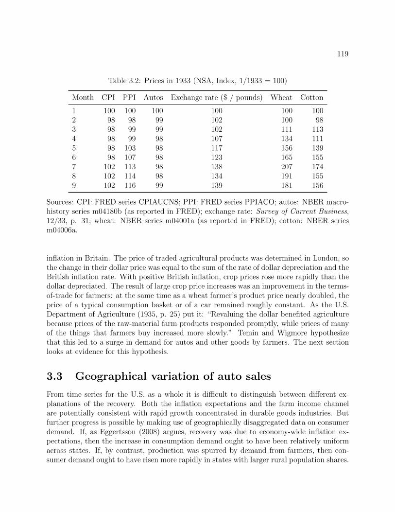
119

Table 3.2: Prices in 1933 (NSA, Index, 1/1933 = 100)

Month CPI PPI Autos Exchange rate ($ / pounds) Wheat Cotton

1 100 100 100 100 100 1002 98 98 99 102 100 983 98 99 99 102 111 1134 98 99 98 107 134 1115 98 103 98 117 156 1396 98 107 98 123 165 1557 102 113 98 138 207 1748 102 114 98 134 191 1559 102 116 99 139 181 156

Sources: CPI: FRED series CPIAUCNS; PPI: FRED series PPIACO; autos: NBER macro-history series m04180b (as reported in FRED); exchange rate: Survey of Current Business,12/33, p. 31; wheat: NBER series m04001a (as reported in FRED); cotton: NBER seriesm04006a.

inflation in Britain. The price of traded agricultural products was determined in London, sothe change in their dollar price was equal to the sum of the rate of dollar depreciation and theBritish inflation rate. With positive British inflation, crop prices rose more rapidly than thedollar depreciated. The result of large crop price increases was an improvement in the terms-of-trade for farmers: at the same time as a wheat farmer’s product price nearly doubled, theprice of a typical consumption basket or of a car remained roughly constant. As the U.S.Department of Agriculture (1935, p. 25) put it: “Revaluing the dollar benefited agriculturebecause prices of the raw-material farm products responded promptly, while prices of manyof the things that farmers buy increased more slowly.” Temin and Wigmore hypothesizethat this led to a surge in demand for autos and other goods by farmers. The next sectionlooks at evidence for this hypothesis.

3.3 Geographical variation of auto sales

From time series for the U.S. as a whole it is difficult to distinguish between different ex-planations of the recovery. Both the inflation expectations and the farm income channelare potentially consistent with rapid growth concentrated in durable goods industries. Butfurther progress is possible by making use of geographically disaggregated data on consumerdemand. If, as Eggertsson (2008) argues, recovery was due to economy-wide inflation ex-pectations, then the increase in consumption demand ought to have been relatively uniformacross states. If, by contrast, production was spurred by demand from farmers, then con-sumer demand ought to have risen more rapidly in states with larger rural population shares.

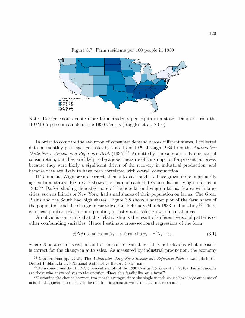
120

Figure 3.7: Farm residents per 100 people in 1930

Note: Darker colors denote more farm residents per capita in a state. Data are from theIPUMS 5 percent sample of the 1930 Census (Ruggles et al. 2010).

In order to compare the evolution of consumer demand across different states, I collecteddata on monthly passenger car sales by state from 1929 through 1934 from the AutomotiveDaily News Review and Reference Book (1935).24 Admittedly, car sales are only one part ofconsumption, but they are likely to be a good measure of consumption for present purposes,because they were likely a significant driver of the recovery in industrial production, andbecause they are likely to have been correlated with overall consumption.

If Temin and Wigmore are correct, then auto sales ought to have grown more in primarilyagricultural states. Figure 3.7 shows the share of each state’s population living on farms in1930.25 Darker shading indicates more of the population living on farms. States with largecities, such as Illinois or New York, had small shares of their population on farms. The GreatPlains and the South had high shares. Figure 3.8 shows a scatter plot of the farm share ofthe population and the change in car sales from February-March 1933 to June-July.26 Thereis a clear positive relationship, pointing to faster auto sales growth in rural areas.

An obvious concern is that this relationship is the result of different seasonal patterns orother confounding variables. Hence I estimate cross-sectional regressions of the form:

%∆Auto salesi = β0 + β1farm sharei + γ′Xi + εi, (3.1)

where X is a set of seasonal and other control variables. It is not obvious what measureis correct for the change in auto sales. As measured by industrial production, the economy

24Data are from pp. 22-23. The Automotive Daily News Review and Reference Book is available in theDetroit Public Library’s National Automotive History Collection.

25Data come from the IPUMS 5 percent sample of the 1930 Census (Ruggles et al. 2010). Farm residentsare those who answered yes to the question “Does this family live on a farm?”

26I examine the change between two-month averages since the single month values have large amounts ofnoise that appears more likely to be due to idiosyncratic variation than macro shocks.

121

Figure 3.8: Change in auto sales and farm share

ALAZ

ARCA

COCT

DE

DCFL

GA

ID

IL

IN

IA

KS

KYLA

ME

MD

MA

MI MNMS

MO

MT

NE

NV

NH

NJ

NM

NY

NC

ND

OH

OK

OR

PARI

SCSD

TN

TXUT

VT

VA

WA

WVWI

WY

020

040

060

0Ch

ange

in a

uto

sale

s, F

eb/M

ar to

Jun

e/Ju

ly 19

33 (%

)

0 20 40 60 80Farm share (%)

Source: See text.

grew most rapidly between March and July 1933. However, seasonally adjusted car salespeaked later, in September, and car sales show substantial month-to-month variability thatmay obscure the macro pattern of interest. Hence I look not only at the change in car salesfrom March to July 1933, but also at the change from the February-March average to theJune-July average, and at the change from the first quarter to the third quarter.

The first three columns of table 3.3 show results from a regression of the percent changein auto sales on the share of a state’s population living on farms and four lags of the changein auto sales. The lags control for the normal seasonal pattern of auto sales in each state.In column 1, the change in auto sales is measured from March to July 1933, in column 2,from the February-March average level of sales to the June-July average, and in column 3,from the first to the third quarter of 1933.

122T

able

3.3:

Auto

sale

sgr

owth

insp

ring

1933

(1)

(2)

(3)

(4)

(5)

(6)

Mar

.to

Ju

l.F

eb.-

Mar.

toJu

n.-

Ju

l.Q

1to

Q3

Mar.

toJu

l.F

eb.-

Mar.

toJu

n.-

Ju

l.Q

1to

Q3

Pop

.sh

are

onfa

rms

1.17

41.7

95**

1.4

80*

2.7

63**

2.6

86***

2.9

57***

(1.1

37)

(0.8

55)

(0.7

51)

(1.3

56)

(0.8

15)

(0.8

67)

1932

∆au

tosa

les

0.72

6*0.6

44*

1.7

55***

(0.4

22)

(0.3

42)

(0.4

75)

1931

∆au

tosa

les

-0.4

36-1

.402**

-1.2

86**

(0.7

98)

(0.5

76)

(0.5

73)

1930

∆au

tosa

les

1.51

7**

1.2

80

0.9

09

(0.7

15)

(0.9

80)

(0.7

22)

1929

∆au

tosa

les

0.21

8-0

.171

0.2

07

(0.3

96)

(0.4

22)

(0.3

29)

Mid

wes

t0.4

30

0.0

928

-0.2

17

(0.6

54)

(0.3

93)

(0.4

18)

Sou

th-0

.251

-0.9

17**

-0.9

09**

(0.6

62)

(0.3

98)

(0.4

23)

Wes

t-0

.104

-0.4

81

-0.6

80*

(0.6

26)

(0.3

76)

(0.4

00)

Con

stan

t1.

235*

**1.1

66***

0.9

54***

0.9

82**

1.3

40***

1.2

56***

(0.3

33)

(0.3

01)

(0.1

86)

(0.4

59)

(0.2

76)

(0.2

93)

Ob

serv

atio

ns

4949

49

49

49

49

R2

0.38

30.3

77

0.5

22

0.1

52

0.3

17

0.2

66

Th

em

axof

conve

nti

onal

and

rob

ust

stan

dard

erro

rsare

inp

are

nth

eses

.*p<.1

0,**

p<.0

5,**

*p<.0

1

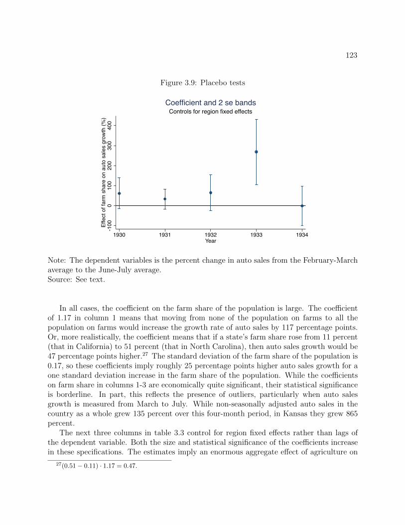
123

Figure 3.9: Placebo tests

-100

010

020

030

040

0Ef

fect

of f

arm

sha

re o

n au

to s

ales

gro

wth

(%)

1930 1931 1932 1933 1934Year

Controls for region fixed effectsCoefficient and 2 se bands

Note: The dependent variables is the percent change in auto sales from the February-Marchaverage to the June-July average.Source: See text.

In all cases, the coefficient on the farm share of the population is large. The coefficientof 1.17 in column 1 means that moving from none of the population on farms to all thepopulation on farms would increase the growth rate of auto sales by 117 percentage points.Or, more realistically, the coefficient means that if a state’s farm share rose from 11 percent(that in California) to 51 percent (that in North Carolina), then auto sales growth would be47 percentage points higher.27 The standard deviation of the farm share of the population is0.17, so these coefficients imply roughly 25 percentage points higher auto sales growth for aone standard deviation increase in the farm share of the population. While the coefficientson farm share in columns 1-3 are economically quite significant, their statistical significanceis borderline. In part, this reflects the presence of outliers, particularly when auto salesgrowth is measured from March to July. While non-seasonally adjusted auto sales in thecountry as a whole grew 135 percent over this four-month period, in Kansas they grew 865percent.

The next three columns in table 3.3 control for region fixed effects rather than lags ofthe dependent variable. Both the size and statistical significance of the coefficients increasein these specifications. The estimates imply an enormous aggregate effect of agriculture on

27(0.51 − 0.11) · 1.17 = 0.47.

124

car sales in spring 1933. One way to see this is to consider what the coefficient implies for acounterfactual world in which the U.S. had zero farm share of the population in 1933. Since25 percent of the population lived on farms,28 a coefficient of 2.7 means that a farm channelaccounted for 68 percentage points29 of overall auto sales growth in the U.S., or roughlyhalf of actual auto sales growth in the period. This calculation should be taken more asan illustration of the scale of the effect rather than as an exact quantitative measure, bothbecause the coefficient is sensitive to the controls (columns 1-3 versus 4-6) and because thecoefficient from a cross-state regression may be a poor measure of the aggregate effect. Ireturn to the latter issue in the next section.

A natural question is whether auto sales always grew more rapidly in spring in states withlarge populations living on farms. If so, this would suggest that the preceding evidence is notin fact indicative of a specific farm channel in the economy’s 1933 recovery. If farm states sawmore rapid auto sales growth in years when there was no dollar devaluation or change in cropprices, then the preceding results would not be evidence about the effects of these policies inspring 1933. Figure 3.9 shows coefficients and two standard error bands from placebo tests,regressions of spring auto sales growth on farm share for each year from 1930 to 1934. Thelarge, statistically significant effect on auto sales growth is unique to 1933. This is strongevidence that the relationship between agriculture and auto sales growth reflects somethingspecific to the 1933 recovery rather than a general relationship between agriculture and autosales.

3.4 Implications

The above results show that auto sales increased more in agricultural than in non-agriculturalareas in spring 1933. While this fact is consistent with Temin and Wigmore’s farm incomehypothesis, there are other stories that could explain higher growth of rural consumption. Adefinitive explanation of differential urban and rural consumption growth in spring 1933 isbeyond the scope of this paper. But in this section I consider two possibilities: (1) a channelthrough farm income and (2) a channel running from higher crop prices to lower farm debtand healthier rural banks.

Farm income

As discussed in the introduction, Temin and Wigmore argue that dollar devaluation ledto higher crop prices and thus higher current and expected income for farmers. This, inturn, led to a rise in farmers’ consumption demand, particularly for autos. This hypothesisfits well with the above evidence on the geographic dispersion of car sales growth in spring1933. Less clear is whether, as Temin and Wigmore suggest, a farm income channel canexplain a significant part of the aggregate economy’s recovery. The problem is that insofar

28IPUMS 5 percent sample of the 1930 Census (Ruggles et al. 2010).290.25 · 2.7 = 0.68

125

Figure 3.10: Expected price increases for shoes

Source: The Warsaw Union, 5/3/1933, p. 2.

as higher farm product prices made farmers richer, they ought also to have made otherspoorer. If higher farm prices were passed through to higher food prices, they made urbanworkers poorer. If they were not passed through, they lowered the profits of food wholesalersand manufacturers. Whether through poorer urban workers or lower profits, higher farmincomes and consumption demand ought to have been matched by lower urban income andconsumption demand. Thus the channel leading from farm prices to farm income couldexplain the much larger growth in car sales in farm states without explaining any of thenationwide growth in car sales in spring 1933. Sales could have risen a lot in North Dakotaand fallen slightly in New York with no net aggregate effect.

How can one break this symmetry between the benefits of higher farm prices for farmersand the costs for non farmers? One plausible possibility are different marginal propensitiesto consume. If non farmers had lower marginal propensities to consume than farmers, atransfer of income from non farmers to farmers would have had overall expansionary effects.It seems unlikely, however, that marginal propensities to consume were sufficiently differentfor this to channel to have produced large aggregate effects.30

30A related hypothesis is that the larger positive effects on farm incomes were more salient than thesmaller negative effects on urban incomes. Insofar as farmers noticed and responded to their higher incomesand urban workers did not notice and did not respond to their lower incomes, this could have lead higherfarm product prices to have positive aggregate effects.

126

Figure 3.11: Expected price increases for tires

Source: Los Angeles Times, 5/11/1933, p. 5.

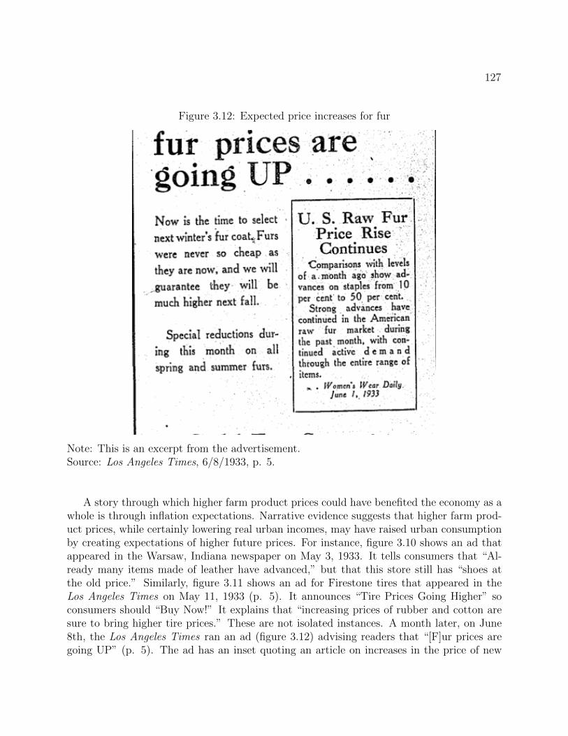
127

Figure 3.12: Expected price increases for fur

Note: This is an excerpt from the advertisement.Source: Los Angeles Times, 6/8/1933, p. 5.

A story through which higher farm product prices could have benefited the economy as awhole is through inflation expectations. Narrative evidence suggests that higher farm prod-uct prices, while certainly lowering real urban incomes, may have raised urban consumptionby creating expectations of higher future prices. For instance, figure 3.10 shows an ad thatappeared in the Warsaw, Indiana newspaper on May 3, 1933. It tells consumers that “Al-ready many items made of leather have advanced,” but that this store still has “shoes atthe old price.” Similarly, figure 3.11 shows an ad for Firestone tires that appeared in theLos Angeles Times on May 11, 1933 (p. 5). It announces “Tire Prices Going Higher” soconsumers should “Buy Now!” It explains that “increasing prices of rubber and cotton aresure to bring higher tire prices.” These are not isolated instances. A month later, on June8th, the Los Angeles Times ran an ad (figure 3.12) advising readers that “[F]ur prices aregoing UP” (p. 5). The ad has an inset quoting an article on increases in the price of new

128

furs.While a definitive argument awaits more systematic work, these advertisements suggest

that higher commodity prices may have caused expected inflation. Since at least Hamilton(1992), economists have known that commodity prices provide information on expectedinflation. My hypothesis goes further: in spring 1933 higher commodity prices not onlyprovide evidence of expected inflation, but, I suggest, were themselves a source of expectedinflation. This points to an interpretation of expected inflation in 1933 somewhat differentfrom that of Eggertsson (2008). Whereas Eggertsson argues that Roosevelt’s words and fiscalactions were crucial since they signalled a commitment to higher inflation, this narrativeevidence suggests a more mechanical possibility: As the dollar weakened, commodity pricesrose. This in turn led consumers to expect broader inflation.

An expansion of Temin and Wigmore’s hypothesis follows: As commodity prices advancedin spring 1933, the consumption of farmers rose along with their permanent income. Atthe same time, real urban incomes fell. Initially, however, the depressing effect on urbanconsumption from lower incomes was balanced by higher consumption spending in advanceof expected price increases. This explanation has the virtue of explaining both the veryrapid recovery in spring 1933 and the subsequent pause in recovery in summer and fall 1933.If consumers brought forward purchases in expectation of higher prices, this would explainwhy recovery faltered after proceeding rapidly. Expectations of price increases would havemeant more shoes, tires and fur coats sold in spring 1933 and fewer sold in summer and fall.That intertemporal substitution in response to expected price increases could have significantmacro effects is made more plausible by the evidence in the previous chapter. There I showedthat expectations of higher car prices contributed to the severity of the 1937-38 recession byshifting car purchases forward to 1937 from 1938.

Farm debt and bank failures

A complementary explanation of the farm consumption boom in spring 1933 is the effect ofhigher farm prices on farm debt burdens and rural banks. Although Temin and Wigmoredo not consider this hypothesis, it is a plausible channel through which higher farm productprices spurred overall recovery.

An astonishing 45 percent of farm owners at the beginning of 1933 were delinquent onmortgage debt (Bernanke 1983). This strained rural banks. The effect was to restrict creditmore in agricultural areas than elsewhere during the Depression (USDA 1935). Higher farmproduct prices promised to allow farmers to service this debt, thus improving the prospectsof rural banks. As Business Week put it in their first issue after Roosevelt abandoned thegold standard (4/26/33, cover page), “70-cent wheat makes a lot of sick banks well again.”31

If, as seems likely, the state of rural banks meant that higher farm product prices improvedrural bank health more than they hurt urban bank health, then this is a channel through

31Wheat prices averaged 52 cents a bushel in March 1933, 63 cents a bushel in April, and 73 cents abushel in May (NBER macrohistory series m04001a).

129

which improved agricultural terms-of-trade may have helped the economy overall. To obtainsome evidence on this channel I estimate the following regression:

%∆Auto salesi = β0 + β1farm sharei + β2bank suspensionsi+ β3farm sharei · bank suspensionsi + γ′Xi + εi, (3.2)

where bank suspensions is a measure of bank distress in state i and Xi is a vector of controlvariables. I measure bank distress as the total number of commercial bank suspensions from1930 to 1932 in a state as a share of the number of commercial banks in a state in 1929. Dataare from the Federal Reserve’s 1943 Banking and Monetary Statistics.32 β3 is the coefficientof interest. It measures whether the effect of farm share on auto sales growth was largerin states with more banking problems. A positive coefficient would suggest that improvingbank conditions in rural states was part of the explanation for the spring 1933 growth of carsales in those states.

Table 3.4 shows results for six specifications. The first two columns use the change incar sales from February-March to June-July as the dependent variable and include lags ofthe dependent variable to control for seasonality. Columns three and four instead controlfor region fixed effects. In all four specifications the coefficient of interest on the interactionterm is measured imprecisely. The econometric problem is multicollinearity: there are only 49observations and the interaction term has a correlation of over 0.8 with both bank distress andfarm share. At the cost of a more difficult to interpret coefficient, the final two columns avoidthe multicollinearity problem by dropping the non-interaction terms from the regression.Interestingly, the interaction of farm share and bank suspensions alone has less explanatorypower than farm share alone. The R2 in columns 5 and 6 is 0.20 and 0.12 versus 0.32 and0.27 when the same specifications are run with farm share alone (see columns 5 and 6 oftable 3.3).

Large standard errors make precise conclusions difficult. But these results provide atleast weak evidence against the view that improving rural bank health was the mechanismbehind rapid auto sales growth in agricultural areas. Thus a channel through farm incomemay have been more important.

32Data on the number of banks in 1929 come from table 8, pp. 24-32; data on the number of banksuspensions from 1930 to 1932 come from table 67, p. 284.

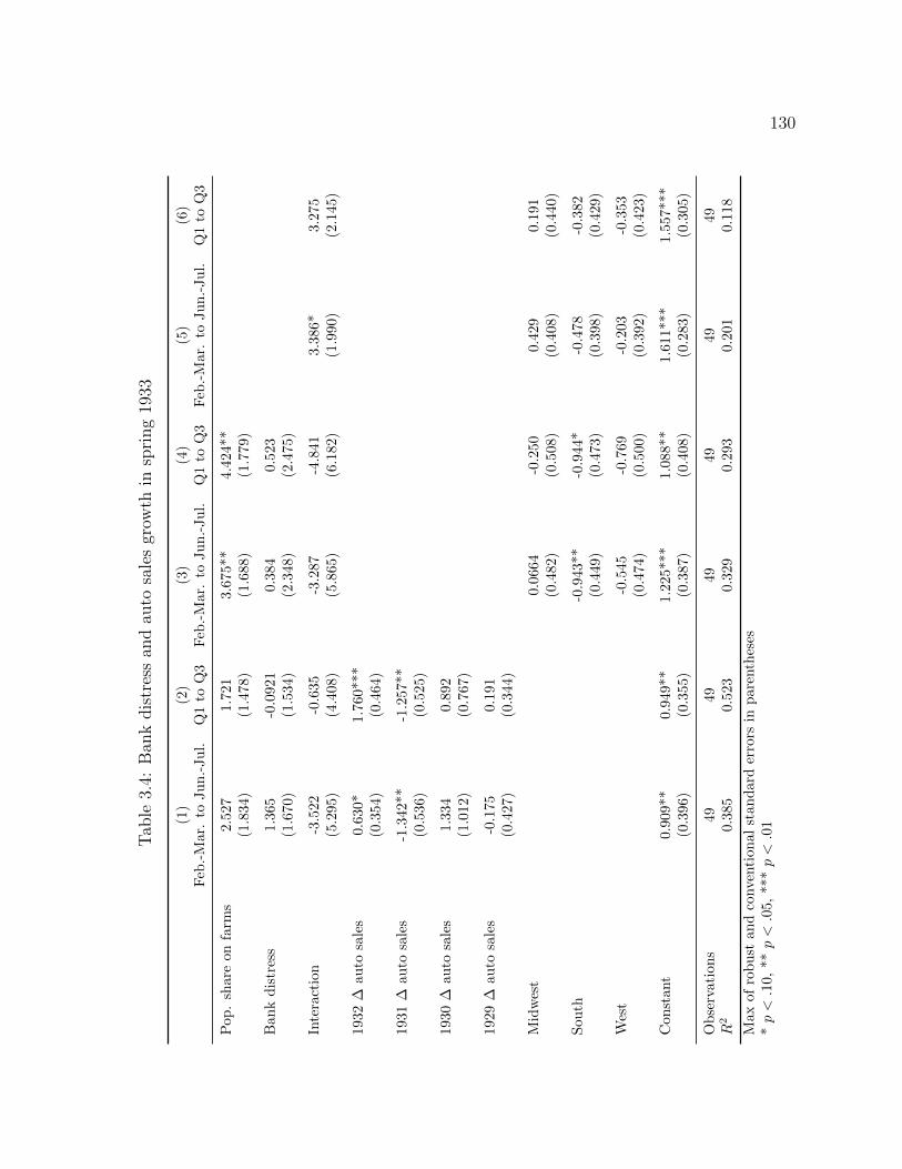
130

Tab

le3.

4:B

ank

dis

tres

san

dau

tosa

les

grow

thin

spri

ng

1933

(1)

(2)

(3)

(4)

(5)

(6)

Feb

.-M

ar.

toJu

n.-

Ju

l.Q

1to

Q3

Feb

.-M

ar.

toJu

n.-

Ju

l.Q

1to

Q3

Feb

.-M

ar.

toJu

n.-

Ju

l.Q

1to

Q3

Pop

.sh

are

onfa

rms

2.52

71.7

21

3.6

75**

4.4

24**

(1.8

34)

(1.4

78)

(1.6

88)

(1.7

79)

Ban

kd

istr

ess

1.36

5-0

.0921

0.3

84

0.5

23

(1.6

70)

(1.5

34)

(2.3

48)

(2.4

75)

Inte

ract

ion

-3.5

22-0

.635

-3.2

87

-4.8

41

3.3

86*

3.2

75

(5.2

95)

(4.4

08)

(5.8

65)

(6.1

82)

(1.9

90)

(2.1

45)

1932

∆au

tosa

les

0.63

0*1.7

60***

(0.3

54)

(0.4

64)

1931

∆au

tosa

les

-1.3

42**

-1.2

57**

(0.5

36)

(0.5

25)

1930

∆au

tosa

les

1.33

40.8

92

(1.0

12)

(0.7

67)

1929

∆au

tosa

les

-0.1

750.1

91

(0.4

27)

(0.3

44)

Mid

wes

t0.0

664

-0.2

50

0.4

29

0.1

91

(0.4

82)

(0.5

08)

(0.4

08)

(0.4

40)

Sou

th-0

.943**

-0.9

44*

-0.4

78

-0.3

82

(0.4

49)

(0.4

73)

(0.3

98)

(0.4

29)

Wes

t-0

.545

-0.7

69

-0.2

03

-0.3

53

(0.4

74)

(0.5

00)

(0.3

92)

(0.4

23)

Con

stan

t0.

909*

*0.9

49**

1.2

25***

1.0

88**

1.6

11***

1.5

57***

(0.3

96)

(0.3

55)

(0.3

87)

(0.4

08)

(0.2

83)

(0.3

05)

Ob

serv

atio

ns

4949

49

49

49

49

R2

0.38

50.5

23

0.3

29

0.2

93

0.2

01

0.1

18

Max

ofro

bust

and

conven

tion

alst

and

ard

erro

rsin

pare

nth

eses

*p<.1

0,**

p<.0

5,**

*p<.0

1

131

3.5 Conclusion

This chapter provides evidence on the sources of U.S. recovery in spring 1933. One viewis that higher expected inflation drove the recovery (Eggertsson 2008). Another is thatdevaluation raised farm incomes, stimulating demand for autos and other goods in ruralareas. This paper provides the high-frequency geographically disaggregated data necessaryto test whether auto sales in fact rose more rapidly in mostly agricultural states. They did.A one standard deviation increase in the share of a state’s population living on farms wasassociated with roughly a 25 percentage point increase in auto sales growth from late winterto early summer 1933.

What explains the disproportionately rapid recovery in rural areas? Temin and Wigmoreargue that devaluation, through its effect on the relative price of farm products, raisedagricultural income. While this argument could explain the geographic pattern of autosales, it is unlikely to explain overall recovery. The positive effect on farm income of highercrop prices ought to have been balanced by a negative effect of higher crop prices on urbanincomes.

I considered two possible ways in which this symmetry may have been broken, in which thepositive effect on farmers may have been larger than the negative effect on urban workers.First, I argued that higher crop prices were not only an indicator of expected inflation(Hamilton 1992), but may also have been a cause of expected inflation. Insofar as highercrop prices raised expected inflation throughout the economy, this relative price change couldhave increased consumption in urban as well as rural areas.

Second, I considered whether higher crop prices had particularly large effects in rural areasby eroding farm debt burdens and thus improving rural bank health. I find no evidence forthis channel. Agricultural states with more bank suspensions during the Depression recoveredno more quickly in spring 1933.

132

Conclusion

This dissertation is a work of economic history. It contributes to our understanding of rapidrecovery and renewed recession during the New Deal. But the lessons are not only historical.As of this writing, in 2013, the developed world is mired in a period of high unemploymentthat has no parallel since the Great Depression. One cannot think about the macroeconomicsof the 1930s without considering lessons for economists and policymakers today. Conversely,policymakers have almost unavoidably sought analogies for their actions in the events of the1930s (Eichengreen 2012).

For fiscal policy, analogies have been lacking. The conventional wisdom is that littlefiscal policy was undertaken in the 1930s and hence that little could be learned about fiscalpolicy from the 1930s. In the first chapter I showed that there was in fact a large fiscalpolicy program in 1936. In June 1936, the U.S. government paid World War I veteransover 2 percent of GDP. As a share of GDP, this is as large as the 2009 American Recoveryand Reinvestment Act (the Obama stimulus). Since the 1936 payment went to World WarI veterans, the typical recipient received a large payment; the average amount was $550dollars, slightly more than contemporary per capita income.

I look at four sources of evidence on the bonus’s effects: a household consumption survey,cross-state and cross-city regressions, an American Legion survey of veterans’ spending plans,and the aggregate time series. These sources paint a consistent picture in which veteransspent the majority of the bonus. From the household consumption survey, I estimate amarginal propensity to consume of 0.7. Combined with a reasonable estimate of the spendingmultiplier, this implies that the bonus added 2.5 to 3 percentage points to 1936 GDP growth.

Would the bonus have been equally effective at other times? Perhaps not. Several featuresof the 1936 economy were uniquely conducive to large effects from a transfer payment.Liquidity constraints were pervasive and were made binding by expectations of higher futureincome. Stocks of autos and housing were low, so many households chose to buy a car orhouse rather than save their bonus. And since the economy was in a liquidity trap, thespending multiplier is likely to have been high.

This argument suggests that the MPC and therefore the aggregate effects of governmenttransfers can depend as much on the state of the economy as on the structure of the payment.The period after a business cycle trough could well be when transfer payments have thelargest effects, since recipients may expect higher future incomes and are anxious to replaceold durables. Conversely, transfer payments may not be the ideal policy tool at the beginning

133

of recessions, since recipients may then fear declines in income and are less likely to need toreplace durables. Periods when liquidity constraints are widespread and unemployment ishigh but falling may well be when fiscal transfers will have the greatest bang for the buck.Future work ought to test this hypothesis.

Fortunately, the double-dip recession of 1937-38 has not (yet) been a relevant analogyfor the U.S. Unfortunately, the same cannot be said for Europe. What can economists andpolicy-makers learn from this interruption to recovery in the 1930s? The conventional wis-dom is that contractionary macro policy, particularly monetary policy, caused the recession.Economists often use the specter of 1937-38 to argue against austerity.33

In the first part of chapter two, I showed that macropolicy cannot account for timing,sectoral, and geographic features of the recession. I argue that an exogenous supply shock inthe auto industry explains these anomalies as well as the recession’s extraordinary severity.The famous American Keynesian Alvin Hansen concludes his book on the 1937-38 recession(1938, p. 274): “Peculiarly, in the year 1938 a conjuncture of circumstances, partly acci-dental, combined to produce the recession.” Hansen was not writing of the auto shock, butunderstanding this shock confirms his point. No successful explanation of 1937-38 is likely tobe monocausal. The coincidence of monetary and fiscal contraction with a large output andprice decline points to the primary importance of aggregate demand. But an understandingof exogenous developments in the auto industry is needed to explain the recession’s timing,geographic and sectoral incidence, and severity. Policymakers today are wise to focus on thedangers of contractionary policy, but they should not ignore industry-specific developments.Likewise, economists would do well to study how supply and demand shocks can interact tocause macroeconomic volatility.

Spring 1933 provides a more optimistic reference for policy. It suggests that even whennominal rates are at zero, the right policy can cause rapid growth. With only aggregate data,however, it has been difficult to disentangle what policy was responsible for the economy’sremarkable turn-around. This chapter makes progress by exploiting monthly state-level autosales data. If, as Eggertsson (2008) argues, the primary shock was an increase in inflationexpectations with no distinct link to agriculture, then one might expect a relatively uniformrecovery of consumer demand across states. If, by contrast, the key shock was the effect ofdollar devaluation on farm product prices, as Temin and Wigmore (1990) argue, then onewould expect to see a more rapid recovery in agricultural states. In fact, the data suggestthe latter. A one-standard deviation increase in the share of the population living on farmswas associated with roughly a 25 percentage point increase in the growth rate of auto salesin a state. It would be useful for future work to explain why farm states recovered so muchmore quickly. I hypothesize that higher farm product prices benefited rural areas throughthe farm income channel identified by Temin and Wigmore and also benefited the entireeconomy through their effect on inflation expectations.

This dissertation is unified not only by themes but also by methodology. Throughout, I

33See, for instance, Christina Romer’s June 2009 column in The Economist entitled “The Lessons of1937.”

134

use disaggregated data to shed light on macro questions. I examine the micro implicationsof macro hypotheses: if the veterans’ bonus was effective, households with veterans ought tohave spent more; if an auto shock contributed to the 1937-38 recession, employment ought tohave fallen most in Michigan; and if higher crop prices contributed to recovery in spring 1933,recovery ought to have proceeded most rapidly in agricultural states. Of course, such microtests are no panacea. The challenge is often to interpret what the micro results say aboutthe macro question. What does a household level marginal propensity to consume revealabout the aggregate effect of the veterans’ bonus? What might the geographical dispersionof auto sales say about aggregate recovery in spring 1933? The mapping from the micro datato such macro questions often requires further assumptions. But while inevitably subject todebate, this approach has great promise for future research.

135

References

Adda, Jerome and Russell Cooper. 2000. “Balladurette and Juppette: A Discrete Analysisof Scrapping Subsidies.” Journal of Political Economy, 108:4, pp. 778-806.

Agarwal, Sumit, Chunlin Liu, and Nicholas S. Souleles. 2007. “The Reaction of ConsumerSpending and Debt to Tax Rebates–Evidence from Consumer Credit Data.” Journal ofPolitical Economy, 115:6, pp. 986-1019.

Alter, Jonathan. 2007. The Defining Moment: FDR’s Hundred Days and the Truimph ofHope. New York: Simon and Schuster.

Alumnia, Miguel, Agustin Benetrix, Barry Eichengreen, Kevin H. O’Rourke, and GiselaRua. 2010. “Lessons from the Great Depression.” Economic Policy, 25:62, pp. 220-265.

Angrist, Joshua D. and Alan B. Krueger. 1992. “The Effect of Age at School Entry onEducational Attainment: An Application of Instrumental Variables with Moments fromTwo Samples.” Journal of the American Statistical Association, 87:418, pp. 328-336.

Aso, Taro. 2013. “Japan is Fighting Back at Stagnation.” Financial Times, April 18.

Automotive Industries. Various issues. Philadelphia: The Chilton Co.

Barro, Robert J. and Chaipat Sahasakul. 1986. “Average Marginal Tax Rates from SocialSecurity and the Individual Income Tax.” Journal of Business, 59:4, pp. 555-566.

Barsky, Robert B., Christopher L. House, and Miles S. Kimball. 2007. “Sticky-Price Modelsand Durable Goods.” American Economic Review, 97:3, pp. 984-998.

Beney, Ada M. 1936. Wages, Hours, and Employment in the United States, 1914-36. NewYork: National Industrial Conference Board.

Berger, David and Joseph Vavra. 2012. “Consumption Dynamics During Recessions.” Work-ing Paper.

Bernanke, Ben. 1983. “Nonmonetary Effects of the Financial Crisis in the Propagation ofthe Great Depression.” American Economic Review, 73:3, pp. 257-276.

136

Bernanke, Ben, and Martin Parkinson. 1989. “Unemployment, Inflation, and Wages in theAmerican Depression: Are There Lessons for Europe?” American Economic Review, 79:2,pp. 210-214.

Blanchard, Olivier, and Roberto Perotti. 2002. “An Empirical Characterization of the Dy-namic Effects of Changes in Government Spending and Taxes on Output.” Quarterly Jour-nal of Economics, 117:4, pp. 1329-1368.

Brown, E. Cary. 1956. “Fiscal Policy in the ’Thirties: A Reappraisal.” American EconomicReview, 46:5, pp. 857-879.

Bureau of Labor Statistics. 1938. Statistics of Building Construction, 1920 to 1937. Bulletin650. Washington, Government Printing Office.

Bureau of Labor Statistics. 1939. Family Income and Expenditure in Chicago, 1935-36:Volume I, Family Income. Washington: Government Printing Office.

Bureau of Labor Statistics. 1940. Building Construction, 1921 to 1938. Bulletin 668. Wash-ington: Government Printing Office.

Bureau of Labor Statistics. 1941a. Family Expenditures in Selected Cities, 1935-36: VolumeI, Housing. Washington: Government Printing Office.

Bureau of Labor Statistics. 1941b. Family Expenditures in Selected Cities, 1935-36: VolumeVIII, Changes in Assets and Liabilities. Washington: Government Printing Office.

Bureau of Labor Statistics. “Full Employment Patterns, 1950.” Undated and unpublished.

Busse, Meghan R., Devin G. Pope, Jaren C. Pope, and Jorge Silva-Risso. 2012. “ProjectionBias in the Car and Housing Markets.” Working Paper.

Calomiris, Charles W., Joseph Mason, and David Wheelock. 2011. “Did Doubling ReserveRequirements Cause the Recession of 1937-1938? A Microeconomic Approach.” NBERWorking Paper 16688.

Card, David and Brian P. McCall. 1996. “Is Workers’ Compensation covering uninsuredmedical costs? Evidence from the Monday effect.” Industrial and Labor Relations Review,49:4, pp. 690-706.

Chandler, Lester V. 1970. America’s Greatest Depression 1929-1941. New York: Harperand Row.

Chow, Gregory. C. and An-Loh Lin. 1971. “Best Linear Unbiased Interpolation, Distri-bution, and Extrapolation of Times Series by Related Series.” Review of Economics andStatistics, 53:4, pp. 372-375.

137

Christiano, Lawrence, Martin Eichenbaum, and Sergio Rebelo. 2011. “When is the Govern-ment Spending Multiplier Large?” Journal of Political Economy, 119:1, pp. 78-121.

Cole, Harold L. and Lee E. Ohanian. 2001. “New Deal Policies and the Persistence of theGreat Depression: A General Equilibrium Analysis.” Federal Reserve Bank of MinneapolisWorking Paper 597.

Cole, Harold L. and Lee E. Ohanian. 2004. “New Deal Policies and the Persistence of theGreat Depression: A General Equilibrium Analysis.” Journal of Political Economy, 112:4,pp. 779-816.

Cole, Harold L. and Lee E. Ohanian. 2009. “How Government Prolonged the Depression.”Wall Street Journal, February 2, p. A17.

Cone, Frederick M. 1940. “Monthly Income Payments in the United States, 1929-40.” U.S.Department of Commerce, Bureau of Foreign and Domestic Commerce, Economic SeriesNo. 6. Washington, DC: Government Printing Office.

Cooper, Russell and John Haltiwanger. 1993. “Automobiles and The National IndustrialRecovery Act: Evidence on Industry Complementarities.” Quarterly Journal of Economics,108:4, pp. 1043-1071.

Costa, Dora L. 1998. The Evolution of Retirement: An American Economic History.Chicago: University of Chicago Press.

Costa, Dora L. 1999. “American Living Standards: Evidence from Recreational Expendi-tures.” NBER Working Paper 7148.

Council of Economic Advisers. 2010. Economic Report of the President. Washington, DC:Government Printing Office.

Crum, W.L., R.A. Gordon, and Dorothy Wescot. 1938. “Review of the Year 1937.” Reviewof Economics and Statistics, 20:1, pp. 43-52.

Daniels, Roger. 1971. The Bonus March: An Episode of the Great Depression. Westport,CT: Greenwood Publishing.

Darby, Michael R. 1976. “Three-and-a-Half Million U.S. Employees have been Mislaid: Or,an Explanation of Unemployment, 1934-1941.” Journal of Political Economy, 84:1, pp. 1-16.

Deaton, Angus. 1997. The Analysis of Household Surveys. Baltimore, MD: The Johns Hop-kins University Press.

DeLong, J. Bradford, and Lawrence H. Summers. 1988. “How does Macroeconomic PolicyAffect Output?” Brookings Papers on Economic Activity, 1988:2, pp. 433-494.

138

Dickson, Paul and Thomas B. Allen. 2004. The Bonus Army: An American Epic. NewYork: Walker and Company.

Drye, Willie. 2002. Storm of the Century: The Labor Day Hurricane of 1935. Washington,DC: National Geographic.

Economic Intelligence Service of the League of Nations. 1938. World Economic Survey1937/38. Geneva: League of Nations.

Eggertsson, Gauti B. 2008. “Great Expectations and the End of the Depression.” AmericanEconomic Review, 98:4, pp. 1476-1516.

Eggertsson, Gauti B. 2012. “Was the New Deal Contractionary?” American EconomicReview, 102:1, pp. 524-555.

Eggertsson, Gauti B. and Benjamin Pugsley. 2006. “The Mistake of 1937: A General Equi-librium Analysis.” Monetary and Economic Studies.

Eichengreen, Barry. 1992. Golden Fetters. New York: Oxford University Press.

Eichengreen, Barry and Jeffrey Sachs. 1985. “Exchange Rates and Economic Recovery inthe 1930s.” Journal of Economic History, 45:4, pp. 925-946.

Eichengreen, Barry. 2012. “Economic History and Economic Policy.” Journal of EconomicHistory, 72:2, pp. 289-307.

Enders, Walter. 2004. Applied Econometric Time Series. John Wiley and Sons.

Federal Reserve Board of Governors. 1939. “Revised Indexes of Factory Employment Ad-justed for Seasonal Variation.” Federal Reserve Bulletin, October, pp. 878-887.

Federal Reserve Board of Governors. 1940. “New Federal Reserve Index of Industrial Pro-duction.” Federal Reserve Bulletin, August, pp. 753-771 and 825-882.

Federal Trade Commission. 1939. Annual Report of the Federal Trade Commission.

Field, Alexander J. 1992. “Uncontrolled Land Development and the Duration of the De-pression in the United States.” Journal of Economic History, 52:4, pp. 785-805.

Field, Alexander J. 2011. A Great Leap Forward: 1930s Depression and U.S. EconomicGrowth. New Haven: Yale University Press.

Fishback, Price V. and Valentina Kachanovskaya. 2010. “In Search of the Multiplier forFederal Spending in the States During the Great Depression.” NBER Working Paper 16561.

Friedman, Milton and Anna Jacobson Schwartz. 1963. A Monetary History of the UnitedStates, 1867-1960. Princeton, NJ: Princeton University Press.

139

Gabaix, Xavier. 2011. “The Granular Origins of Aggregate Fluctuations.” Econometrica,79:3, pp. 733-772.

Galenson, Walter. 1960. The CIO Challenge to the AFL: A History of the American LaborMovement 1935-41. Cambridge, MA: Harvard University Press.

Gates, Paul W. 1977. “Homesteading in the High Plains.” Agricultural History, 51:1, pp.109-133.

General Motors. 1937. Annual Report of General Motors Corporation, Year Ended December31, 1936.

Gordon, Robert J. and Robert Krenn. 2010. “The End of the Great Depression 1939-41:Policy Contributions and Fiscal Multipliers.” NBER Working Paper 16380.

Gordon, Robert J. and John M. Veitch. 1986. “Fixed Investment in the American BusinessCycle, 1919-83,” in The American Business Cycle: Continuity and Change, Robert J.Gordon, ed. Chicago: University of Chicago Press for NBER, pp. 267-335.

Hall, Robert E. 2009. “By How Much Does GDP Rise if the Government Buys MoreOutput?” Brooking Papers on Economic Activity, fall, pp. 183-249.

Hansen, Alvin Harvey. 1938. Full Recovery or Stagnation? New York: W.W. Norton andCompany.

Heasley, Jerry. 1977. The Production Figure Book for U.S. Cars. Osceola, WI: MotorbooksInternational.

Hemingway, Ernest. 1935. “Who Murdered the Vets?: A First-Hand Report on the FloridaHurricane.” New Masses, September 17.

Hicks, J.R. 1937. “Mr. Keynes and the ‘Classics’; A Suggested Interpretation.” Economet-rica, 5:2, pp. 147-159.

Horner, S. L. 1939. “Statement of the Problem” in The Dynamics of Automobile Demand.New York: General Motors Corporation, pp. 3-18.

House, Christopher L., and John V. Leahy. 2004. “An sS Model with Adverse Selection.”Journal of Political Economy, 112:3, pp. 581-614.

Hsieh, Chang-Tai. 2003. “Do Consumers React to Anticipated Income Changes? Evidencefrom the Alaska Permanent Fund.” American Economic Review, 93:1, pp. 397-405.

Hymans, Saul H., Joan P. Crary, E. Philip Howrey, and Janet C. Wolfe. 2002. The MichiganEconometric Model of the U.S. Economy.

140

Inoue, Atsushi, and Gary Solon. 2010. “Two-sample Instrumental Variables Estimators.”Review of Economics and Statistics, 92:3, pp. 557-561.

Irwin, Douglas A. 2011. “Gold Sterilization and the Recession of 1937-38.” DartmouthCollege Working Paper.

Johnson, David S., Jonathan A. Parker, and Nicholas S. Souleles. 2006. “Household Ex-penditure and the Income Tax Rebates of 2001.” American Economic Review, 96:5, pp.1589-1610.

Kashyap Anil K. and David W. Wilcox. 1993. “Production and Inventory Control at theGeneral Motors Corporation During the 1920’s and 1930’s.” American Economic Review,83:3, pp. 383-401.

Keynes, John Maynard. 1964 [1936]. The General Theory of Employment, Interest, andMoney. New York: Harcourt, Brace and World.

Kimball, Miles. 2012. “Getting the Biggest Bang for the Buck in Fiscal Policy.” WorkingPaper, University of Michigan.

Kindleberger, Charles. 2013 [1973]. The World in Depression 1929-1939. Berkeley, CA:University of California Press.

Krugman, Paul R. 1998. “It’s Baaack: Japan’s Slump and the Return of the LiquidityTrap.” Brookings Papers on Economic Activity, 1998:2, pp. 137-205.

Lebergott, Stanley. 1964. Manpower in Economic Growth; the American Record since 1800.New York: McGraw-Hill.

Leontief, Wassily. 1951. The Structure of American Economy, 1919-1939; An EmpiricalApplication of Equilibrium Analysis. New York: Oxford University Press.

Lewis, W. Arthur. 1949. Economic Survey, 1919-1939. London: G. Allen and Unwin.

Long, John B. and Charles I. Plosser. 1987. “Sectoral vs. Aggregate Shocks in the BusinessCycle.” American Economic Review, 77:2, pp. 333-336.

Lusardi, Annamaria. 1996. “Permanent Income, Current Income, and Consumption: Evi-dence from Two Panel Data Sets.” Journal of Business and Economic Statistics, 14:1, pp.81-90.

Mendel, Brock. 2012. “The Local Multiplier: Theory and Evidence.” Working Paper, Har-vard University.

Mishkin, Frederic S. “The Household Balance Sheet and the Great Depression.” 1978.Journal of Economic History, 38:4, pp. 918-937.

141

Nakamura, Emi and Jon Steinsson. 2011. “Fiscal Stimulus in a Monetary Union: Evidencefrom U.S. Regions.” NBER Working Paper 17391.

Natural Resources Committee. 1939. Consumer Expenditures in the United States. Wash-ington, DC: Government Printing Office.

Olney, Martha L. 1991. Buy Now Pay Later: Advertising, Credit, and Consumer Durablesin the 1920s. Chapel Hill, NC: University of North Carolina Press.

Olney, Martha L. 1999. “Avoiding Default: The Role of Credit in the Consumption Collapseof 1930.” Quarterly Journal of Economics, 114:1, pp. 319-335.

Ortiz, Stephen R. 2010. Beyond the Bonus March and the GI Bill: How Veteran PoliticsShaped the New Deal Era. New York: New York University Press.

Parker, Jonathan A., Nicholas S. Souleles, David S. Johnson, and Robert McClelland. 2011.“Consumer Spending and the Economic Stimulus Payments of 2008.” NBER Working Paper16684.

Raff, Daniel M.G., and Manuel Trajtenberg. 1996. “Quality-Adjusted Prices for the Amer-ican Automobile Industry: 1906-1940,” in The Economics of New Goods, Timothy F. Bres-nahan and Robert J. Gordon, eds. Chicago: University of Chicago Press, pp. 71-108.

Ramey, Valerie A. 2011. “Can Government Purchases Stimulate the Economy?” Journalof Economic Literature, 49:3, pp. 673-685.

Ramey, Valerie A. and Daniel J. Vine. 2006. “Declining Volatility in the U.S. AutomobileIndustry.” American Economic Review, 96:5, pp. 1876-1889.

Reinhart, Carmen M. and Kenneth S. Rogoff. 2009. This Time is Different: Eight Centuriesof Financial Folly. Princeton, NJ: Princeton University Press.

Reinhart, Carmen M. and Kenneth S. Rogoff. 2010. “After the Fall.” NBER Working Paper16334.

Roberts, Phil. A New History of Wyoming. University of Wyoming online document.

Rockoff, Hugh. 2001. “The Changing Role of America’s Veterans.” NBER Working Paper8595.

Romer, Christina D. 1986. “New Estimates of Prewar Gross National Product and Unem-ployment.” Journal of Economic History, 46:2, pp. 341-352.

Romer, Christina D. 1989. “The Prewar Business Cycle Reconsidered: New Estimates ofGross National Product, 1869-1908.” Journal of Political Economy, 97:1, pp. 1-37.

142

Romer, Christina D. 1990. “The Great Crash and the Onset of the Great Depression,”Quarterly Journal of Economics, 105:3, pp. 597-624.

Romer, Christina D. 1992. “What Ended the Great Depression?” Journal of EconomicHistory, 52:4, pp. 757-784.

Romer, Christina D. 1994. “Remeasuring Business Cycles.” Journal of Economic History,54:3, pp. 573-609.

Romer, Christina D. 2013. “It Takes a Regime Shift: Recent Developments in JapaneseMonetary Policy Through the Lens of the Great Depression.” Revised version of speach pre-sented at the NBER Annual Conference on Macroeconomics on April 12. Availabile at http://elsa.berkeley.edu/~cromer/It%20Takes%20a%20Regime%20Shift%20Written.pdf.

Roos, C.F. and Victor Von Szeliski. 1939. “Factors Governing Changes in Domestic Au-tomobile Demand” in The Dynamics of Automobile Demand. New York: General MotorsCorporation, pp. 21-95.

Roose, Kenneth D. 1954. The Economics of Recession and Revival: An Interpretation of1937-38. New Haven, CT: Yale University Press.

Roth, Benjamin. 2009. The Great Depression: A Diary. James Ledbetter and Daniel B.Roth, eds. New York: Public Affairs.

Rowlands, David T. 1943. “Land and Homes for Returning Servicemen.” Annals of theAmerican Academy of Political and Social Science, 227, pp. 143-151.

Ruggles, Steven, J. Trent Alexander, Katie Genadek, Ronald Goeken, Matthew B.Schroeder, and Matthew Sobek. 2010. Integrated Public Use Microdata Series: Version5.0 [Machine-Readable database]. Minneapolis: University of Minnesota.

Sayre, R. A. 1940. “Wages, Hours, and Employment in the United States, 1934-39.” TheConference Board Economic Record, II:10.

Shapiro, Matthew D. and Joel Slemrod. 2003. “Consumer Response to Tax Rebates.” Amer-ican Economic Review, 93:1, pp. 381-396.

Shapiro, Matthew D. and Joel Slemrod. 2009. “Did the 2008 Tax Rebates Stimulate Spend-ing?” American Economic Review, 99:2, pp. 374-379.

Shaw, William Howard. 1947. Value of Commodity Output since 1869. New York: NationalBureau of Economic Research.

Shefrin, Hersh M. and Richard H. Thaler. 1988. “The Behavioral Life-Cycle Hypothesis.”Economic Inquiry, XXVI, pp. 609-643.

143

Souleles, Nicholas S. 1999. “The Response of Consumption to Income Tax Refunds.” Amer-ican Economic Review, 89:4, pp. 947-958.

Suits, Daniel B. 1958. “The Demand for New Automobiles in the United States.” Reviewof Economics and Statistics, 40:3, pp. 273-280.

Survey of Current Business. 1934. “Index of Sales of New Passenger Automobiles.” April,pp. 16-19.

Svensson, Lars E. O. 2003. “Escaping from a Liquidity Trap and Deflation: The FoolproofWay and Others.” Journal of Economic Perspectives, 17:4, pp. 145-166.

Telser, Lester G. 2003-2004. “The Veterans’ Bonus of 1936.” Journal of Post-KeynesianEconomics, 26:2, pp. 227-243.

Temin, Peter and Barrie A. Wigmore. 1990. “The End of One Big Deflation.” Explorationsin Economic History, 27, pp. 483-502.

Tobin, James. 1958. “Estimation of Relationships for Limited Dependent Variables.” Econo-metrica, 26:1, pp. 24-36.

Treasury Department. 1936. Annual Report of the Secretary of the Treasury on the State ofthe Finances For Fiscal Year ended June 30, 1936.

Troy, Leo. 1957. “Union Membership, 1939 and 1953,” in Distribution of Union Membershipamong the States, 1939 and 1953, ed. Leo Troy.

United States Department of Agriculture. 1935. Yearbook of Agriculture. Washington, DC:Government Printing Office.

United States Department of Labor. Bureau of Labor Statistics. Cost of Living Division,United States Department of Agriculture. Bureau of Home Economics. Economics Division ,United States National Resources Committee. Consumption Research Staff. Industrial Sec-tion, United States Central Statistical Board, and United States Works Progress Adminis-tration. 2009. Study of Consumer Purchases in the United States, 1935-1936. ICPSR08908-v3. Ann Arbor, MI: Inter-university Consortium for Political and Social Research [distrib-utor], 2009-06-29. doi:10.3886/ICPSR08908.v3

Velde, Francois R. 2009. “The Recession of 1937–A Cautionary Tale.” Economic Perspec-tives, 33, pp. 16-37.

Veterans’ Administration. Various years. Annual Report of the Administrator of Veterans’Affairs for the Fiscal Year ended June 30. Washington, DC: Government Printing Office.

Wallis, John Joseph. 1989. “Employment in the Great Depression: New Data and Hypothe-ses.” Explorations in Economic History, 26, pp. 45-72 .

144

Ward’s Reports Inc. 1938. Ward’s 1938 Automotive Year Book. Detroit: Ward’s ReportsInc.

Werning, Ivan. 2012. “Managing a Liquidity Trap: Monetary and Fiscal Policy.” MITWorking Paper.

Woodford, Michael. 2011. “Simple Analytics of the Government Expenditure Multiplier.”American Economic Journal: Macroeconomics, 3, pp. 1-35.

Woodford, Michael. 2012. “Methods of Policy Accommodation at the Interest-Rate LowerBound.” Working Paper, Columbia University.