Embed Size (px)
Citation preview

New Deal Policies and the Persistence of the Great Depression: A General Equilibrium AnalysisAuthor(s): Harold L. Cole and Lee E. OhanianSource: The Journal of Political Economy, Vol. 112, No. 4 (Aug., 2004), pp. 779-816Published by: The University of Chicago PressStable URL: http://www.jstor.org/stable/3555138Accessed: 05/04/2010 15:16
Your use of the JSTOR archive indicates your acceptance of JSTOR's Terms and Conditions of Use, available athttp://www.jstor.org/page/info/about/policies/terms.jsp. JSTOR's Terms and Conditions of Use provides, in part, that unlessyou have obtained prior permission, you may not download an entire issue of a journal or multiple copies of articles, and youmay use content in the JSTOR archive only for your personal, non-commercial use.
Please contact the publisher regarding any further use of this work. Publisher contact information may be obtained athttp://www.jstor.org/action/showPublisher?publisherCode=ucpress.
Each copy of any part of a JSTOR transmission must contain the same copyright notice that appears on the screen or printedpage of such transmission.
JSTOR is a not-for-profit service that helps scholars, researchers, and students discover, use, and build upon a wide range ofcontent in a trusted digital archive. We use information technology and tools to increase productivity and facilitate new formsof scholarship. For more information about JSTOR, please contact [email protected].
The University of Chicago Press is collaborating with JSTOR to digitize, preserve and extend access to TheJournal of Political Economy.
http://www.jstor.org
New Deal Policies and the Persistence of the Great Depression: A General Equilibrium Analysis
Harold L. Cole University of California, Los Angeles
Lee E. Ohanian University of California, Los Angeles, Federal Reserve Bank of Minneapolis, and National Bureau of Economic Research
There are two striking aspects of the recovery from the Great De- pression in the United States: the recovery was very weak, and real wages in several sectors rose significantly above trend. These data contrast sharply with neoclassical theory, which predicts a strong re- covery with low real wages. We evaluate the contribution to the per- sistence of the Depression of New Deal cartelization policies designed to limit competition and increase labor bargaining power. We develop a model of the bargaining process between labor and firms that oc- curred with these policies and embed that model within a multisector dynamic general equilibrium model. We find that New Deal carteli- zation policies are an important factor in accounting for the failure of the economy to recover back to trend.
I. Introduction
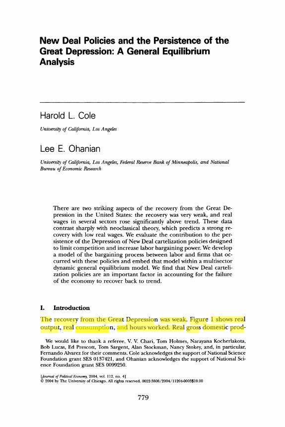
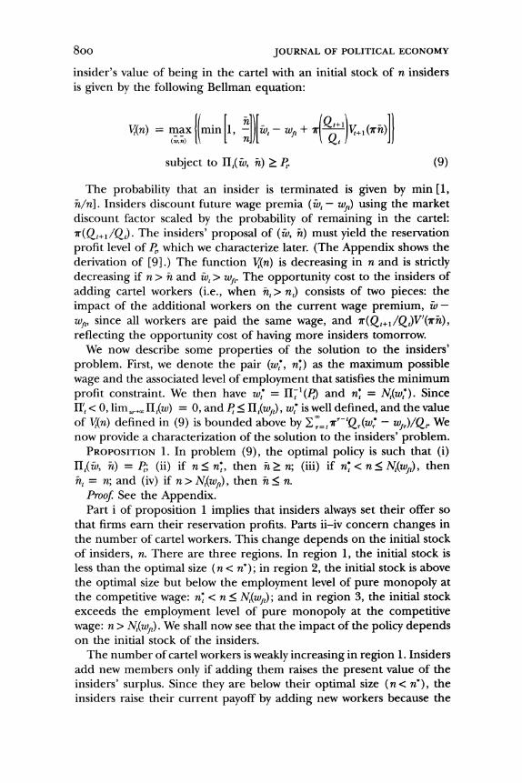
The recovery from the Great Depression was weak. Figure 1 shows real
output, real consumption, and hours worked. Real gross domestic prod-
We would like to thank a referee, V. V. Chari, Tom Holmes, Narayana Kocherlakota, Bob Lucas, Ed Prescott, Tom Sargent, Alan Stockman, Nancy Stokey, and, in particular, Fernando Alvarez for their comments. Cole acknowledges the support of National Science Foundation grant SES 0137421, and Ohanian acknowledges the support of National Sci- ence Foundation grant SES 0099250.
[ournal of Political Economy, 2004, vol. 112, no. 4] ? 2004 by The University of Chicago. All rights reserved. 0022-3808/2004/11204-0003$10.00
779

100 -
90
" 80 ON \ \ Consumption - -
70
GDP
60 1929 1930 1931 1932 1933 1934 1935 1936 1937 1938 1939
Year
FIG. 1.-Real GDP and consumption per adult (deviations from trend)
uct per adult, which was 39 percent below trend at the trough of the
Depression in 1933, remained 27 percent below trend in 1939. Similarly, private hours worked were 27 percent below trend in 1933 and remained 21 percent below trend in 1939. The weak recovery is puzzling because the large negative shocks that some economists believe caused the 1929- 33 downturn-including monetary shocks, productivity shocks, and banking shocks-become positive after 1933. These positive shocks should have fostered a rapid recovery, with output and employment returning to trend by the late 1930s.1
Some economists suspect that President Franklin Roosevelt's "New Deal" cartelization policies, which limited competition in product mar- kets and increased labor bargaining power, kept the economy depressed after 1933 (see Friedman and Schwartz 1963; Alchian 1970; Lucas and
Rapping 1972). These policies included the National Industrial Recov-
ery Act (NIRA), which suspended antitrust law and permitted collusion in some sectors provided that industry raised wages above market-clear-
ing levels and accepted collective bargaining with independent labor unions. Despite broad and long-standing interest in the macroeconomic impact of these policies, there are no theoretical general equilibrium models tailored to study this question.
This paper develops a theoretical model of these policies and uses it to quantitatively evaluate their macroeconomic effects. We construct a
dynamic model of the intraindustry bargaining process between labor and firms that occurred under these policies and embed this bargaining model into a multisector dynamic general equilibrium model. The model differs from existing insider-outsider models in a number of ways. One key difference is that our model allows the insiders to choose the size of the worker cartel, which lets us study the impact of the policies in a much richer way than in existing models. We simulate the model
during the New Deal and compare output, employment, consumption, investment, wages, and prices from the model to the data. Our main
finding is that New Deal cartelization policies are a key factor behind the weak recovery, accounting for about 60 percent of the difference between actual output and trend output.
The paper is organized as follows. Section II presents macroeconomic data for the 1930s. Section III discusses the New Deal policies and com- pares wage and price changes from industries covered by the policies to those from industries not covered by the policies. Section IV develops
The monetary base increases more than 100 percent between 1933 and 1939, the introduction of deposit insurance ends banking panics by 1934, and total factor produc- tivity returns to trend by 1936. Lucas and Rapping (1972) argue that positive monetary shocks should have produced a strong recovery, with employment returning to its normal level by 1936. Cole and Ohanian (1999) make a similar argument about positive produc- tivity and banking shocks.
781 NEW DEAL POLICIES
JOURNAL OF POLITICAL ECONOMY
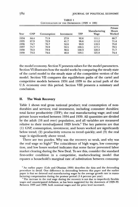
TABLE 1 CONTINUATION OF THE DEPRESSION (1929 = 100)
Private Manufacturing Hours
Year GNP Consumption Investment TFP Wage Worked
1934 64.4 71.9 27.9 92.6 111.1 68.7 1935 67.9 72.9 41.7 96.6 111.2 71.4 1936 74.7 76.7 52.6 99.9 110.5 75.8 1937 75.7 76.9 59.5 100.5 117.1 79.5 1938 70.2 73.9 38.6 100.3 122.2 71.7 1939 73.2 74.6 49.0 103.1 121.8 74.4
the model economy. Section V presents values for the model parameters. Section VI illustrates how the model works by comparing the steady state of the cartel model to the steady state of the competitive version of the model. Section VII compares the equilibrium paths of the cartel and
competitive models between 1934 and 1939 to the actual path of the U.S. economy over this period. Section VIII presents a summary and conclusion.
II. The Weak Recovery
Table 1 shows real gross national product; real consumption of non- durables and services; real investment, including consumer durables; total factor productivity (TFP); the real manufacturing wage; and total
private hours worked between 1934 and 1939. All quantities are divided
by the adult (16 and over) population, and all variables are measured relative to their trend-adjusted 1929 levels.2 The key patterns are that (1) GNP, consumption, investment, and hours worked are significantly below trend; (2) productivity returns to trend quickly; and (3) the real
wage is significantly above trend. There are two puzzles. Why was the recovery so weak, and why was
the real wage so high?3 The coincidence of high wages, low consump- tion, and low hours worked indicates that some factor prevented labor market clearing during the New Deal. To see this, consider the standard first-order condition in a competitive, market-clearing model that
equates a household's marginal rate of substitution between consump-
2An earlier paper (Cole and Ohanian 1999) describes the data and the detrending procedure in detail. One difference in detrending between this paper and the earlier paper is that we detrend real manufacturing wages by the average growth rate in manu- facturing compensation during the postwar period (1.4 percent per year).
3 The increase in the real wage during the recovery is not due to imperfectly flexible wages and unanticipated deflation, as has been suggested for the downturn of 1929-33. Between 1933 and 1939, both nominal wages and the price level increased.
782

tion and leisure to the real wage. With log preferences over consumption (c) and leisure (1), the first-order condition is ct/l, = wr
There is a large gap in this condition during the New Deal. Compared to 1929 values, the 1939 real wage is 120 percent higher than the 1939 marginal rate of substitution. Competition should have generated higher employment, higher consumption, and a lower real wage to reduce this large gap. A successful theory of the New Deal macroecon- omy should account for the weak recovery, the high real wage, and the large gap between the marginal rate of substitution between consump- tion and leisure and the real wage.
III. New Deal Labor and Industrial Policies
Roosevelt's recipe for economic recovery was raising prices and wages. To achieve these increases, Congress passed industrial and labor policies to limit competition and raise labor bargaining power. This section summarizes Roosevelt's economic views and policies and shows that prices and wages rose substantially after these policies were adopted.
There were two policy phases during the New Deal. The first phase was the NIRA (1933-35). The NIRA created rents by limiting compe- tition and allowed labor to capture some of those rents by exempting industry from antitrust prosecution if the industry immediately raised wages and accepted collective bargaining with labor unions.
The second policy phase was adopted after the Supreme Court ruled the NIRA unconstitutional in 1935. The court's NIRA decision pre- vented Roosevelt from tying collusion to paying high wages, so instead the government largely ignored the antitrust laws and passed the Na- tional Labor Relations Act (NLRA), which strengthened several of the NIRA's labor provisions. We present data that show very little antitrust prosecution by the Department of Justice (DOJ) after 1935 and show that the government openly ignored collusive arrangements in indus- tries that paid high wages. We also present data that systematically show that wages and prices continued to rise after the court struck down the NIRA. We now describe those policies and summarize their key features.
A. The NIRA
Roosevelt believed that the severity of the Depression was due to ex- cessive business competition that reduced prices and wages, which in turn lowered demand and employment. He argued that government planning was necessary for recovery:
A mere builder of more industrial plants, a creator of more railroad systems, an organizer of more corporations, is as likely
783 NEW DEAL POLICIES

JOURNAL OF POLITICAL ECONOMY
to be a danger as a help. Our task is not ... necessarily pro- ducing more goods. It is the soberer, less dramatic business of
administering resources and plants already in hand. [Quoted in Kennedy (1999, p. 373)]
A number of Roosevelt's economic advisors, who had worked as eco- nomic planners during World War I, argued that wartime economic
planning would bring recovery. HughJohnson, one of Roosevelt's main economic advisors, argued that the economy expanded during World War I because the government ignored the antitrust laws. According to Johnson (1935), this policy reduced industrial competition and conflict, facilitated cooperation between firms, and raised wages and output. This wartime policy was the model for the NIRA.
The cornerstone of the NIRA was a "code of fair competition" for each industry. These codes were the operating rules for all firms in an
industry. Firms and workers negotiated these codes under the guidance of the National Recovery Administration (NRA). The codes required presidential approval, which was given only if the industry raised wages and accepted collective bargaining with an independent union. In re- turn, the act suspended antitrust law, and each industry was encouraged to adopt trade practices that limited competition and raised prices. By 1934, NRA codes covered over 500 industries, which accounted for
nearly 80 percent of private, nonagricultural employment.4 All codes adopted a minimum wage for low-skilled workers, and almost
all codes specified higher wages for higher-skilled workers (see Lyon et al. 1935). A significant element of the wage provisions was wage unifor- mity: employees performing the same job were paid the same wage. Consequently, codes generally did not permit wage discrimination based on seniority or other criteria (see, e.g., the petroleum code in National Recovery Administration [1933-35, 1:151]).
Most industry codes included trade practice arrangements that limited
competition, including minimum prices; restrictions on production, in- vestment in plant and equipment, and the workweek; resale price main- tenance; basing point pricing; and open-price systems.5 Minimum price was the most widely adopted provision, and the code authority often determined the minimum price in many industries. Several codes per- mitted the code authority to set industrywide or regional minimum
4 The private, nonagricultural sectors exempted from the NIRA were steam railroads, nonprofit organizations, domestic services, and professional services.
5 Open-price systems required that any firm planning to reduce its price must pre- announce the action to the code authority, who in turn would notify all other firms. Following this notification, the announcing firm was required to wait a specific period before changing its price. The purpose of this waiting period was for the code authority and other industry members to persuade the announcing firm to cancel its price cut.
784
NEW DEAL POLICIES 785
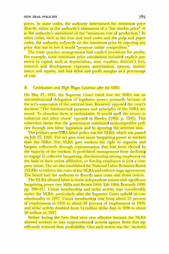
prices. In some codes, the authority determined the minimum price directly, either as the authority's assessment of a "fair market price" or as the authority's assessment of the "minimum cost of production." In other codes, such as the iron and steel codes and the pulp and paper codes, the authority indirectly set the minimum price by rejecting any price that was so low it would "promote unfair competition."
The trade practice arrangements had explicit provisions for profits. For example, some minimum price calculations included explicit pay- ments to capital, such as depreciation, rent, royalties, director's fees, research and development expenses, amortization, patents, mainte- nance and repairs, and bad debts and profit margins as a percentage of cost.
B. Cartelization and High Wages Continue after the NIRA
On May 27, 1935, the Supreme Court ruled that the NIRA was an unconstitutional delegation of legislative power, primarily because of the act's suspension of the antitrust laws. Roosevelt opposed the court's decision: "The fundamental purposes and principles of the NIRA are sound. To abandon them is unthinkable. It would spell the return to industrial and labor chaos" (quoted in Hawley [1966, p. 124]). This subsection shows that the government continued anticompetitive poli- cies through new labor legislation and by ignoring the antitrust laws.
The primary post-NIRA labor policy was the NLRA, which was passed on July 27, 1935. The act gave even more bargaining power to workers than the NIRA. The NLRA gave workers the right to organize and bargain collectively through representation that had been elected by the majority of the workers. It prohibited management from declining to engage in collective bargaining, discriminating among employees on the basis of their union affiliation, or forcing employees to join a com-
pany union. The act also established the National Labor Relations Board (NLRB) to enforce the rules of the NLRA and enforce wage agreements. The board had the authority to directly issue cease and desist orders.
The NLRA allowed labor to form independent unions with significant bargaining power (see Millis and Brown 1950; Taft 1964; Kennedy 1999, pp. 290-91). Union membership and strike activity rose considerably under the NLRA, particularly after the Supreme Court upheld its con-
stitutionality in 1937. Union membership rose from about 13 percent of employment in 1935 to about 29 percent of employment in 1939, and strike activity doubled from 14 million strike days in 1936 to about 28 million in 1937.
Strikes during the New Deal were very effective because the NLRA allowed workers to take unprecedented actions against firms that sig- nificantly reduced firm profitability. One such action was the "sit-down
JOURNAL OF POLITICAL ECONOMY
strike," in which strikers forcibly occupied factories and halted produc- tion. The sit-down strike was used with considerable success against auto and steel producers (see Kennedy 1999, pp. 310-17). The NLRA con- trasts sharply with pre-New Deal government strike policy, in which
government injunctions or police action was frequently used to break strikes.
The uniform wage feature of NIRA labor policies continued in post- NIRA union contracts.6 The strengthening of NIRA labor provisions was
accompanied by an NIRA-type industrial policy that promoted collusion. Even though the government could not suspend antitrust law after the NIRA, the government permitted collusion, particularly in industries that paid high wages. Hawley (1966, p. 166) cites Federal Trade Com- mission (FTC) studies from the 1930s that report price fixing and pro- duction limits in a number of industries following the court's NIRA decision.
Some of the post-NIRA collusion was facilitated by trade practices formed under the NIRA. Hawley reports that basing point pricing, which was adopted under the NIRA, allowed steel producers to collude after the act was ruled unconstitutional. Interior Secretary Harold Ickes com-
plained to Roosevelt that he received identical bids from steel firms on 257 different occasions (Hawley 1966, pp. 360-64) between June 1935 and May 1936. The Interior Department received bids that were not
only identical but 50 percent higher than foreign steel prices (Ickes 1953-54, 2:466). This price difference was large enough under govern- ment rules to permit Ickes to order the steel from German suppliers. Roosevelt canceled the German contract, however, after coming under
pressure from both the steel trade association and the steel labor union.
Despite this collusion, the U.S. attorney general announced that steel
producers would not be prosecuted for restraint of trade (Hawley 1966, p. 364). Hawley documents that the steel case was just one example of a lax pattern of post-NIRA antitrust prosecution. Of the few cases that were prosecuted by the DOJ between 1935 and 1937, several involved
alleged racketeering charges.7 The number of antitrust case brought by the DOJ fell from an average of 12.5 new cases per year during the 1920s to an average of 6.5 cases per year during the period 1935-38 (Posner 1970).
6 Ross (1948) and Reynolds and Taft (1955) document that unions established uniform and standardized wage schedules that narrowed wage differentials. (Cole and Ohanian [2001] discuss this issue in greater detail.)
7 New legislation enacted during the mid-1930s is also viewed by some as limiting price competition, including the Robinson-Patman Act (1936), which was designed to prevent firms from selling goods at different prices to different customers, and the Miller-Tydings Act (1937), which exempted resale price maintenance contracts from antitrust laws.
786
C. The End of the New Deal
Roosevelt's views changed in the late 1930s, and his policies also changed. He argued that cartelization was an important contributing factor to the persistence of the Depression and appointed Thurman Arnold, a vigorous antitruster, to reorganize and direct the Antitrust Division of the DOJ. The number of new cases brought by the DOJ rose from just 57 between 1935 and 1939 to 223 between 1940 and 1944. Posner (1970) reports that about 80 percent of these cases were won by the government.
Labor policy also changed significantly. The Supreme Court ruled in 1939 that the sit-down strike was unconstitutional, which weakened la- bor's bargaining power considerably (see Kennedy 1999, pp. 316-17). Bargaining power was further weakened during World War II because
wage increases had to be approved by the National War Labor Board, and this board almost uniformly rejected wage agreements that ex- ceeded cost-of-living increases. Moreover, strikes by coal miners during the war pushed public and congressional opinion against unions and the NLRA. In 1947, the NLRA was amended by the Taft-Hartley Act. This act weakened labor's bargaining power by restricting labor's actions and by reducing the original limitations placed on firms in the original NLRA. The act outlawed the closed shop and gave states the right to outlaw union shops. Given this policy shift, we shall focus our analysis on the 1933-39 period.
D. The Impact of the Policy on Wages and Prices
We now present evidence that New Deal policies significantly increased wages and prices. We compare wage and price statistics in industries covered by the policies to those in industries not covered by the policies. Wage and price data are limited during the 1930s. Given this limitation, we have compiled wage and price statistics that show that real wages and relative prices in sectors covered by the policies rose significantly after the NIRA was adopted and remained high throughout the New Deal. We also show that wages and prices in sectors not covered by these policies did not rise during the New Deal.
We first describe the available wage and price data, and we then classify these data between the cartelized and noncartelized sectors. We have wage data for the overall manufacturing sector and for some industries within manufacturing. We also have wages for some energy industries and for agriculture. We divide nominal wages by the GNP deflator to see whether there were differences in real wage changes across the two categories.
Regarding prices, we have price indexes for the major National In-
787 NEW DEAL POLICIES
JOURNAL OF POLITICAL ECONOMY
TABLE 2 INDEXED REAL WAGES RELATIVE TO TREND
Sector 1930 1931 1932 1933 1934 1935 1936 1937 1938 1939
Manufacturing 101.7 106.3 105.1 102.9 110.8 112.0 111.6 118.9 122.9 123.6 Bituminous coal 101.2 104.8 91.4 90.4 110.1 119.1 125.3 127.8 130.9 132.7 Anthracite coal ... ... 100.0 100.0 92.7 90.3 89.9 89.1 94.1 94.4 Petroleum ... ... 100.0 103.6 108.9 113.6 115.4 124.8 129.1 128.8 Farm 94.6 78.8 63.0 60.9 60.8 64.1 67.7 72.9 68.5 68.6
NOTE.-Wages are deflated by the GNP deflator and a 1.4 percent trend, which is the growth rate of manufacturing compensation in the postwar period. They are indexed to be 100 in 1929, except for the wages in anthracite and petroleum, which are indexed to 1932 = 100 because of data availability.
come and Product Accounts categories and wholesale price indexes for
manufacturing industries and for some energy industries. We divide the nominal price indexes by the price index for consumer services. We choose the price of consumer services as the numeraire because it is the aggregate price index likely to be least affected by the policies, since some consumer services were not covered by the policies and because collusion failed in some services that were covered.8 This procedure of
forming relative prices lets us determine whether cartelized prices rose relative to noncartelized prices (services). To the extent possible, we
report prices and wages for the same industries/sectors. We describe how we divide these sectors between the cartelized and noncartelized
groups below. Table 2 shows annual data for wages in three sectors covered by the
policies-manufacturing, bituminous coal, and petroleum products- and two sectors not covered-anthracite coal and all farm products. The farm sector was not covered by the NIRA, by the NLRA, or by other policies that would have raised farm wages. Anthracite coal is a partic- ularly interesting de facto uncovered sector because it was supposed to have been covered by the NIRA, but the industry and the coal miners failed to negotiate a code of fair competition.
We find that real wages in the three covered sectors rise after the NIRA is adopted and remain high through the rest of the decade. In
comparison to their 1929 levels, manufacturing, bituminous coal, and petroleum wages are between 24 and 33 percent above trend in 1939. In contrast, the farm wage is 31 percent below trend, and anthracite coal is 6 percent below trend. Focusing on the two coal wages, we find that bituminous coal miners-who successfully negotiated under the NIRA-were able to raise their real wage substantially, whereas anthra- cite coal miners-who did not successfully negotiate under the NIRA- were not able to raise their real wage.
8 For example, physician services were not covered by the policies. Other services, such as dry cleaning, were covered, but were found to be very competitive by the NIRA review board (1934).
788
NEW DEAL POLICIES
TABLE 3 MONTHLY WAGES RELATIVE TO THE GNP DEFLATOR (February 1933 = 100)
April December June May December June Industry 1933 1933 1934 1935 1935 1936
Leather tanning 96.6 124.0 122.2 121.9 123.0 124.9 Boots and shoes 104.7 145.9 138.1 139.0 139.7 137.0 Cotton 96.7 142.0 133.2 135.2 133.4 134.3 Iron/steel 100.2 123.1 122.7 124.6 125.0 127.0 Foundaries and ma-
chine shops 99.4 112.6 111.9 113.4 113.6 115.9 Autos 98.9 115.5 121.3 121.0 123.1 125.8 Chemicals 102.8 117.6 118.2 121.5 123.1 124.1 Pulp/paper 100.7 117.5 111.4 115.3 116.4 117.9 Rubber
manufacturing 100.7 121.3 125.9 134.1 137.0 128.6 Furniture 102.3 118.9 125.9 129.2 129.0 130.3 Farm implements 96.5 107.1 105.6 115.3 116.9 113.7
Since the manufacturing wage is an aggregate of many manufacturing industry wages, it is natural to ask whether this increase is due to in- creases across all or most manufacturing industries or whether it is due to very large increases in just a few industries. Using monthly industry- level wage data within manufacturing from the Conference Board (Be- ney 1936; Hanes 1996), we find that all these industry wages significantly increased. We report real wages in 11 manufacturing industries for which we also have price data. Table 3 shows significant increases in all 11 industries occurring after the NIRA is passed. Here, we index the real wage to 100 in February 1933 (which is a few months prior to the passage of the NIRA) to focus on the effect of the adoption of the policies on real wages. All these industry wages are significantly higher at the end of 1933, which is six months after the act is passed. The smallest increase is 7 percent (farm implements), and the largest increase is 46 percent (boots and shoes). These wages also remain high through the end of the NIRA (May 1935) and also after the act was ruled unconstitutional. The average real wage increase across these 11 categories in June 1936 relative to February 1933 is 25.4 percent.
These wage premia in the cartelized sectors are higher than estimates of union wage premia, which some authors have used to gauge labor market distortions.9 There are two key reasons why estimates of union/ nonunion wage premia are not the right statistics for evaluating New Deal wage increases. One is that the NIRA raised wages of union and nonunion workers. Very few workers were even in unions in 1933, and the NIRA took this into account by forcing firms to raise wages of all workers to get cartelization benefits. One example of the quantitative
9 Mulligan (2000) uses these premia to study U.S. labor market distortions.
789
JOURNAL OF POLITICAL ECONOMY
TABLE 4 PRICE OF INVESTMENT GOODS AND FARM GOODS RELATIVE TO PERSONAL CONSUMPTION
SERVICES (1929 = 100)
1930 1931 1932 1933 1934 1935 1936 1937 1938 1939
Fixed investment 96.9 95.1 93.2 99.9 108.3 110.0 109.5 115.0 114.0 112.5 Durable equipment 97.1 98.1 101.8 99.5 110.2 109.6 107.6 111.3 113.4 111.3
importance of this factor comes from Lewis (1963). He analyzed bitu- minous coal wages in regions with different unionization rates and found that wages rose substantially for all states, regardless of the fraction of
employment unionized, with the highest percentage increases occurring in nonunion regions. He also reports a union wage differential of 10- 18 percent in rubber tire manufacturing in 1935. But this statistic does not take into account the fact that overall rubber manufacturing wages- including nonunion wages-rose 35 percent between 1933 and 1935. A second reason that union wage premia are poor estimates of the
impact of New Deal wage increases is that most estimates of union wage premia come from post-World War II data. These data are not good estimates because postwar union bargaining power was lower than worker bargaining power during the New Deal.
We now turn to an analysis of the relative price data. We continue to treat the manufacturing sector and the energy industries described above as the cartelized sectors. We omit the farm sector from this price analysis. We do not include farm goods in the uncovered category for
prices, as we had done for wages, because the government adopted other policies to raise farm prices. However, these price support policies differed significantly from the NIRA since they did not include provi- sions to raise wages.
Regarding the manufacturing sector, we would like to match up a
price index for the overall manufacturing sector with the overall man-
ufacturing wage index reported in table 2. Unfortunately, there is no such price index. We therefore report relative prices of industries within
manufacturing that we can match up with the manufacturing industry wage data reported in table 3, and we also report relative prices of investment goods, which are a major manufactured good. Table 4 shows relative prices of new fixed investment goods and durable equipment goods. These relative prices rise about 8-10 percent between 1934 and 1933 and are about 11-12 percent above their 1929 levels in 1939. These increases are particularly noteworthy because they occur during an eco- nomic recovery. Typically, the relative price of investment goods falls
during recoveries (see Greenwood, Hercowitz, and Krusell 2000). We now turn to the other price data. Table 5 shows the manufacturing
and energy goods prices before and after New Deal policies. We use the
79?

TABLE 5 WHOLESALE PRICES RELATIVE TO THE PERSONAL CONSUMPTION SERVICES DEFLATOR (February 1933 = 100)
December December April 1933 1933 June 1934 May 1935 1935 June 1936 June 1937 June 1938 June 1939
I 1 I I
I
I
I
I I
(,
I
I I P ,4
Leather/hides 102.1 Fextiles 131.8 ?urniture 99.4 11 home furnishings 98.9
knthracite coal 91.8 3ituminous coal 98.4 ?etroleum products 94.8 1hemicals 100.6 )rugs/pharmaceuticals 99.6 ron/steel 97.9 4onferrous metals 106.5 itructural steel 100.0 11 metal products 99.4 tutos 99.4 ?ulp/paper 98.1 tuto tires 87.8 tubber 121.3 'arm equipment 100.0 11 building materials 100.6 tverage* 103.2
* The average does not include rubber.
131.2 149.2 110.3 112.0 91.9
114.1 150.4 100.3 107.7 108.2 144.2 106.2 107.9 100.0 114.4 101.4 295.1 102.4 122.6 117.1
126.1 127.5 137.8 143.8 133.1 140.4 108.1 105.3 105.3 111.6 109.5 109.5 85.3 80.8 91.8
117.8 117.0 119.3 145.2 145.2 142.6 97.9 108.8 108.8
131.3 133.0 133.0 97.0 114.6 108.7
145.9 147.1 147.1 113.8 110.6 110.6 111.5 109.9 110.1 102.9 102.0 102.0 114.0 108.5 108.5 103.0 103.7 103.7 446.9 400.8 400.8 107.9 110.6 118.8 123.8 119.3 119.3 120.0 122.6 123.7
126.7 128.5 143.0 131.9 142.3 116.9 103.9 112.2 106.2 107.9 115.3 110.1 84.1 78.2 76.8
117.8 115.6 112.2 162.4 167.0 150.0 107.8 104.6 99.7 138.6 144.8 127.4 108.2 120.2 119.3 146.8 185.3 133.0 109.7 131.0 126.4 107.9 115.4 113.5
96.5 107.1 122.8 108.4 102.3 123.3 123.2 413.0 626.2 394.1 109.8 105.5 105.7 119.1 129.3 117.5 116.8 124.6 117.9
Industry
121.1 120.1 103.0 108.2 77.8
110.1 139.9 97.4
129.1 112.6 144.2 120.0 110.1 93.5
101.3 129.8 515.5 102.7 117.2 113.8
JOURNAL OF POLITICAL ECONOMY
same format as in table 3 for manufacturing industry wages by choosing the same reporting dates and the same date for the normalization. The
timing and magnitude of the price increases are very similar to those for the other wage and price changes we observe. Prices for almost all the categories covered by the policies rise substantially by the end of 1933 and remain high through the end of the 1930s. It is again inter-
esting to compare the price of bituminous coal-an industry that ne-
gotiated a code of fair competition under the NIRA-to the price of anthracite coal-an industry that did not negotiate a code of fair com-
petition. The relative price of bituminous coal rises after the NIRA is
passed and remains high through 1939. In contrast, the relative price of anthracite coal is unchanged after the NIRA is passed and then declines moderately over the rest of the 1930s.
In summary, we have compiled wage data from manufacturing, energy, mining, and agriculture and price data from these same sectors less
agriculture. This evidence indicates that New Deal policies raised relative prices and real wages in those industries covered by these policies: man-
ufacturing and some energy industries. Relative prices and real wages in these sectors increased significantly after these policies were adopted and remained high throughout the 1930s, whereas prices and wages in uncovered sectors did not rise.
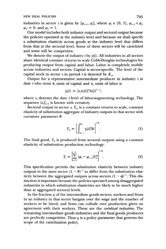
There is additional evidence supporting our conclusions about the effects of these policies. One source of evidence is the National Recovery Review Board (NRRB), which was an independent government agency that evaluated whether the NIRA was creating monopoly. This board was created because of widespread complaints by consumers, businesses, and government purchasing agencies about price fixing and collusion. The NRRB wrote three different reports over the course of the NIRA, analyzing industries covering about 50 percent of NIRA employment. Sixteen of the 26 codes that were studied by the board covered industries that we have classified as cartelized. The NRRB concluded on the basis of trade practices and conduct that there was significant monopoly in all 16 of these industries:'1
Our investigations have shown that in the instances mentioned the codes do not only permit but foster monopolistic practices and nothing has been done to remove or even to restrain them. If monopolistic business combinations in this country could have anything ordered to their wish, they could not order any-
10 The board concluded that most of the remaining 10 industries were also cartelized, but data limitations prevented us from including these industries. The NRRB also con- cluded that the one consumer service it studied-cleaning and dyeing-was very com- petitive, which supports our view that consumer services were less affected by these policies.
792

thing better than to have the antitrust laws suspended. [Na- tional Recovery Review Board 1935, 3d report, pp. 34-37]
There are other sources of evidence supporting our conclusions. One source is a series of FTC analyses of manufacturing industries, which concluded that there was collusion under the NIRA and after it was ruled unconstitutional. The FTC concluded that there was little com-
petition in many concentrated industries, including autos, chemicals, aluminum, and glass.' A second source of evidence is stock market data. The Dow Jones 30 Industrials and the Standard and Poor's In- dustrials rose 74 percent and 100 percent, respectively, between March 1933, before the policy was announced, and July 1933, which was the first month after the policy was adopted."' These indexes remained around their July 1933 levels over the next year as the policy was im-
plemented (source of data: Board of Governors of the Federal Reserve
System [1943] and Pierce [1982]). Stock returns are also consistent with our view that cartelization continued after the NIRA was declared un- constitutional in June 1935. These stock indexes rose about 10 percent between May 1935 and July 1935. Even Roosevelt finally acknowledged the impact of cartelization on the economy by the late 1930s: "the Amer- ican economy has become a concealed cartel system. ... The disap- pearance of price competition is one of the primary causes of present difficulties" (quoted in Hawley [1966, p. 412]).
The evidence indicates that New Deal policies created cartelization, high wages, and high prices in at least manufacturing and some energy and mining industries. Hereafter, we shall treat these industries as car- telized and the remainder of the economy as competitive. We shall then use the relative sizes of these two categories to parameterize the car- telized and competitive sectors of our model. We therefore assume that all the other sectors in the economy for which we do not have price and wage data were unaffected by the policies. This is a conservative estimate of the fraction of the economy that was cartelized, because there is evidence that the policies affected other sectors. (For example, the NRRB found evidence of monopoly in wholesale and retail trade.) We shall show later that our conservative assessment of the size of the cartelized sector will understate the effects of these policies on em-
ployment and output.
1 See Hawley (1966) for a summary of post-NIRA FTC studies that found significant evidence of monopoly in manufacturing.
12 Of the 30 DowJones Industrial companies, 28 were in either manufacturing or energy production, which we classify as cartelized.
793 NEW DEAL POLICIES

IV. A Dynamic General Equilibrium Model with New Deal Policies
Our model of New Deal policy specifies that in a subset of industries, workers and firms bargain over the wage and that the firms can collude over pricing and production if they reach a labor agreement. The anal-
ysis requires developing a new theoretical model because several nec-
essary elements do not jointly appear in existing models. Four key el- ements are (i) repeated bargaining in some sectors, with collusion contingent on the labor agreement; (ii) optimal choice for the number of cartel workers by the insiders; (iii) job search; and (iv) voluntary participation by firms. The first element captures the essence of the NIRA. The second and third elements let us assess the model's predic- tions for employment, unemployment, output, and other macroeco- nomic variables during the New Deal. The fourth element captures the fact that industry was an early supporter of the NIRA. These features-
particularly the optimal determination of the number of insiders-let us analyze the impact of the policies in a much richer way than had we used existing insider-outsider models.'3 With these elements, our model is consistent with key objectives of labor unions during the 1930s, in-
cluding raising wages and eliminating wage differentials across similar workers (see Ross 1948; Reynolds and Taft 1955). Our model also is reminiscent of the classic Harris and Todaro (1970) model in which
unemployment serves as a lottery for high-wage jobs.
A. Environment
Time is discrete and is denoted by t = 1, 2, ..., oo. There is no uncer-
tainty. There is a representative household whose members supply labor and capital services and consume the final good. There are two distinct
types of goods: Final goods can be consumed or invested. These final
goods are produced using a variety of intermediate goods. These inter- mediate goods are produced using identical technologies with capital and labor. There is a unit mass of intermediate goods indexed by i E
[0, 1]. Each i denotes a specific industry. We partition the unit interval of industries into different sectors. There are S sectors, and the set of
13 In addition to the optimal choice of the size of the insiders, the participation decision of the firms is also a novel feature of our model relative to other insider-outsider models, such as those of Blanchard and Summers (1986), Lindbeck and Snower (1988), Gali (1995), and Alvarez and Veracierto (2000). The number of insiders is a parameter in Blanchard and Summers' and Snower and Lindbeck's models. Gali's model is one in which the entire economy is monopolized and thus cannot be used to study a partially cartelized economy, which is the focus of our paper, including cross-sector wage differ- entials or the size of the cartel sector. The most closely related model is that of Alvarez and Veracierto. However, policies have larger negative effects in our model than in theirs because the insiders control the size of their cartel.
794 JOURNAL OF POLITICAL ECONOMY
industries in sector s is given by [p,-_1, s,], where op, E [0, 1], (_p,- < (p,
'Po = 0, and ps = 1. Our model includes both industry output and sectoral output because
the policies operated at the industry level and because we shall specify a substitution elasticity across goods at the industry level that differs from that at the sectoral level. Some of these sectors will be cartelized and some will be competitive.
We denote the output of industry i by y(i). All industries in all sectors share identical constant returns to scale Cobb-Douglas technologies for
producing output from capital and labor. Labor is completely mobile across industries and sectors. Capital is sector-specific. The level of the
capital stock in sector s in period t is denoted by K,. Output for a representative intermediate producer in industry i at
date t who rents kt units of capital and nt units of labor is
t(i) = [ztnt(i)]Ykt(i)'-,
where zt denotes the date t level of labor-augmenting technology. The
sequence {zJtlo is known with certainty. Sectoral output in sector s, Y,, is a constant returns to scale, constant
elasticity of substitution aggregate of industry outputs in that sector with curvature parameter 0:
Ps 1/pS
Y, = y,(i)?di (1) . (OPs-1
The final good, Yt, is produced from sectoral outputs using a constant elasticity of substitution production technology:
.s=
This specification permits the substitution elasticity between industry outputs in the same sector (1 - 0)-1 to differ from the substitution elas- ticity between the aggregated outputs across sectors (1 - )-1. This dis- tinction is important because the policies operated among disaggregated industries in which substitution elasticities are likely to be much higher than at aggregated sectoral levels.
In the fraction X of the intermediate goods sectors, workers and firms in an industry in that sector bargain over the wage and the number of workers to be hired, and firms can collude over production given an agreement with their workers. These are the cartelized industries. The
remaining intermediate goods industries and the final goods producers are perfectly competitive. Thus X is a policy parameter that governs the scope of the cartelization policy.
795 NEW DEAL POLICIES
JOURNAL OF POLITICAL ECONOMY
Symmetry implies that the cartelized sectors and the competitive sec- tors can be aggregated. This lets us work with a two-sector model with a cartel sector of size X and a competitive sector of size 1 - X. We shall use m to refer to cartel sector and f to refer to the competitive sector. The output of the cartel sector is
m . ..f 1/0
Ymt-- IYt0(i)di
The output of the competitive sector is
1/0
Yft yt'(i)di
Final output is the numeraire. We denote the output and its price in a
representative cartelized industry by Ymt and pm, and similarly denote the
output and price in a representative competitive industry by yf and Pf, We also denote the wage rates and capital rental rates in representative industries in the two sectors as wmt and rmt and w, and rf
The fraction of household members nf work in the competitive sector, the fraction nmt work in the cartel sector, the fraction nut search for a
job in the cartel sector, and the remainder take leisure. Since the cartel
wage will be higher than the competitive wage, household members
compete for these rents by searching for cartel jobs. Searching consists of waiting for a vacant cartel job, and search incurs the same utility cost as working full-time. If a cartel job vacancy arises, the job is awarded randomly at the start of the period to an individual who searched the
previous period. We denote the probability of obtaining a cartel job through search in period t as v,.
To build in job turnover arising from life cycle events such as retire- ment or disability, we assume that cartel workers face an exogenous probability of losing theirjobs at each date. The probability that a worker retains his or her cartel job is 1r.14
B. Household Problem
The representative family's problem is
max I 't- [log (ct) + 4 log (1 - n)] (nmb.nutnft t= 1
14 With < 1, there is a unique balanced growth for the model. If X = 1, then the balanced growth path depends on initial conditions.
796

subject to
Qwf, nf + Wmtnmt- Ct + (rstks - x,s) + II = 0, (3)
t=l s=l
kst+l = x,t + (1- 6)ks,, (4)
nmt < rn,,_l + vt-lnu,,t- (5)
nt = nft m+ t+ ,,
where wnm,_, denotes the initial number of insiders in the first period. The household's income consists of flows of labor income from the
competitive and noncompetitive sectors, rental income from supplying capital, and date 1 profits (II1). Equation (5) is the law of motion for the number of household members with cartel jobs (nm). This is equal to the number of household members who retain their cartel jobs from last period (irnmt_l), plus the number of household members who obtain vacant cartel jobs from searching the previous period (v,_in,t_). The term Qt is the date t Arrow-Debreu price of final goods. All the first- order conditions for this problem are standard, with the exception of the first-order condition for searching for a cartel job. This condition is
00
vt-1 Qt+Tr(Wmt+T -
Wft+r) =
Qt-lwt-1? (6) 7=1
This equation shows that the marginal benefit of searching, which is the expected present value of the cartel wage premia, is equal to the
opportunity cost of searching, which is the value of the previous period's wage.
C. Competitive Goods Producers
A representative final goods producer, taking prices of its inputs as given, {pt(i)}, has the following profit maximization problem:
max Y - p,(i)y,(i)di + p,(i)y,(i)di . yt(i)
797 NEW DEAL POLICIES

JOURNAL OF POLITICAL ECONOMY
A representative intermediate goods producer in a competitive in-
dustry maximizes profits given (pf, Wt, rf):
maxpft(ztnft)'kft- - wtnft - rfkfr (7) nfpkft
D. The Cartel
We now describe the maximization problem of cartel workers and cartel firms. The insiders are the workers who were employed in the industry last period and who did not suffer attrition. The insiders bargain each period with the firms in the industry over the wage and the employment level.
The bargaining game between the insiders and the firms is a two-
stage negotiation game that is played at the beginning of the period. In stage 1, the insiders make a wage and employment proposal: (W,, nt). (In equilibrium, it will be the case that w, = wmt and h, = nmr) In
stage 2, the firms either accept or reject this proposal. If the firms accept it, they collude and operate as a monopolist, subject to the constraint that they hire nt units of labor at the wage wt, hiring first from the stock of insiders. If the firms reject the proposal, they hire labor from the spot market at the competitive spot market wage, wft. In this case, how- ever, firms can collude and operate as a monopolist only with probability o. With probability 1 - o, firms must behave competitively. Thus this parameter governs the probability that the government enforces anti- trust law when firms do not pay high wages.
To characterize the equilibrium, we shall first conjecture that the firms play a reservation profits strategy in the bargaining game. We then derive the insiders' best response to this strategy by setting up their dynamic programming problem. We shall then verify that the conjectured strat-
egy for the firms is a best response to the strategy that solves the insiders' maximization problem.
We first define the firm's profit function. For any arbitrary wage w and exogenous variables Y,, Ym, Zt, and rmt, profits are given by
,I(w) = max{Ytl-'Ym ,-[(ztn)k'-Y]' - rmtk - wn}, (8) n,k
where we have used the inverse demand function of the final goods producers to construct the revenue function for the industry; 1/(1 - 4) and 1/(1 - 0) are the substitution elasticities over sectoral goods in final goods output and industry goods in sectoral output, respectively. The associated optimal employment function is given by Nt(w) = n. We shall use IIt(w, n) as the solution to the monopolist's maximization prob- lem when he rents the optimal quantity of capital, taking wages and
798

employment as given. We shall later use these functions when we con- struct the solution to the bargaining game.
1. The Insiders' Problem
The existing stock of insiders in an industry is given by n. They make a sequence of wage/employment offers to the firms in the industry to maximize the expected present value of the wage premium per insider. If the insiders' offer of (w, n) is accepted, everyone hired in the car- telized industry receives the same wage, w, and the hiring rule within the cartel is as follows. If n > n, then all the insiders get jobs and n - n workers are hired randomly from the cartel job searchers.'5 If n < n, then n - n of the insiders are randomly chosen to leave the industry, and those remaining get jobs. A key aspect of the proposal is wage uniformity between insiders and new hires, which is motivated by the uniform wages paid during the New Deal.'6
Note that with an accepted agreement, insiders control entry into their group and exit (net of attrition) from their group. Moreover, insiders add new members only if the insiders' payoffs are increased, since insiders do not care about the welfare of new members. Once new members are added, however, they become insiders the following period.
Since insiders are perfectly insured within the family and because
they can always work at the competitive wage, they maximize the ex-
pected present value of the premium between the cartel wage and the
competitive wage. Moreover, given perfect family insurance, it is optimal that insiders who are terminated or who suffer exogenous attrition re- ceive no insurance payments."7
The value of being an insider is the expected present value of the cartel wage premia. We assume that the firms will accept any wage and employment offer (,w, n,) that promises the firms at least their reser- vation profits Pt. Given this reservation profit constraint, an individual
15 If all the job searchers are hired, then any additional workers are hired randomly from the pool of nonsearchers.
16 Given the absence of wage discrimination, the marginal cost of an additional worker in the cartel sector (w,,) exceeds that in the competitive sector (wp). This wage premium reduces the employment level below the employment level that would prevail if the cartel could pay the marginal worker a wage less than w,,
7 We assume that families are large enough to insure members against employment risk but small enough that family members work in only a small fraction of the cartelized industries. This assumption implies that the family does not internalize the aggregate consequences of its members' actions since the likelihood that a family member obtains a cartel job is independent of the actions of the industries in which family members work.
799 NEW DEAL POLICIES
JOURNAL OF POLITICAL ECONOMY
insider's value of being in the cartel with an initial stock of n insiders is given by the following Bellman equation:
V(n) = max min 1, - wt- t + tr V V+i (rn)
(w,nsubject n.(, ) P (9)
subject to IIt( w, h) > P,. (9)
The probability that an insider is terminated is given by min [1, n/n]. Insiders discount future wage premia (w, - wf) using the market discount factor scaled by the probability of remaining in the cartel:
7r(Qt+/Q,t). The insiders' proposal of (w, n) must yield the reservation
profit level of P, which we characterize later. (The Appendix shows the derivation of [9].) The function Vt(n) is decreasing in n and is strictly decreasing if n > n and wt > wft. The opportunity cost to the insiders of
adding cartel workers (i.e., when nt> nt) consists of two pieces: the
impact of the additional workers on the current wage premium, w -
Wft, since all workers are paid the same wage, and r(Q,t+/Q,)V'(rit), reflecting the opportunity cost of having more insiders tomorrow.
We now describe some properties of the solution to the insiders'
problem. First, we denote the pair (w*, n*) as the maximum possible wage and the associated level of employment that satisfies the minimum
profit constraint. We then have wt = HII(Pt) and nt = Nt(wt). Since II' < 0, lim,o II,(w) = 0, and Pt < II(wft), w* is well defined, and the value of V,(n) defined in (9) is bounded above by S r=tr-'Q,(w - wf,)/Qt. We now provide a characterization of the solution to the insiders' problem.
PROPOSITION 1. In problem (9), the optimal policy is such that (i) fIt(w, n) = Pt; (ii) if n < n, then n 2 n; (iii) if n< < n < N,(w%), then nt = n; and (iv) if n > N,(wt), then n < n.
Proof. See the Appendix. Part i of proposition 1 implies that insiders always set their offer so
that firms earn their reservation profits. Parts ii-iv concern changes in the number of cartel workers. This change depends on the initial stock of insiders, n. There are three regions. In region 1, the initial stock is less than the optimal size (n < n*); in region 2, the initial stock is above the optimal size but below the employment level of pure monopoly at the competitive wage: n; < n < Nt(wft); and in region 3, the initial stock exceeds the employment level of pure monopoly at the competitive wage: n > N(wft). We shall now see that the impact of the policy depends on the initial stock of the insiders.
The number of cartel workers is weakly increasing in region 1. Insiders add new members only if adding them raises the present value of the insiders' surplus. Since they are below their optimal size (n< n*), the insiders raise their current payoff by adding new workers because the
8oo
fixed cost of paying PJ can be spread among more members. In this
region, this cost reduction more than offsets the fall in the marginal revenue product of adding new workers in this region. The weakly in-
creasing aspect of this result arises because n+s, may be below n*. Sim-
ilarly, the weakly decreasing aspect of part iv arises because ns,, could be greater than nt.
Region 2 is a zone of inactivity with no employment change, despite the fact that the number of insiders exceeds the optimal number. The reason that the insiders choose not to shrink is that this action would reduce the insiders' current expected surplus per member, because
shrinking their size would reduce the total surplus available to the in- siders and because total rents are maximized at Nt(wf,). Thus the insiders
keep employment constant because any change would reduce their ex-
pected payoff. Employment is weakly decreasing in region 3 because in this region
the group is sufficiently large that it earns no current surplus above the
competitive wage. Thus insiders may choose to shrink their membership. The employment level at which insiders choose to shed workers depends on the attrition probability parameter and the discount factor. With attrition, new workers will ultimately be added. This means that keeping employment constant, rather than shrinking employment, may be op- timal because it postpones the date at which new members would be admitted and thus lets current members receive the future surplus that would otherwise be paid to the new hires.
2. The Firm's Best Response
Here we verify our conjecture that, given the insiders' strategy, the firms'
optimal strategy is to accept any offer (wt, nt) that yields profits of at least wIIt(wt). To do so, conjecture that the continuation payoff to the firms from period t + 1 onward is given by
Wt+1 Q Cii,(wf). (10) r=t+l .t+l
Note that this payoff is independent of the number of workers in the
industry at the beginning of period t + 1. Next, consider what happens if firms reject the workers' offer in period t. With probability w they behave as a monopolist hiring labor at the competitive wage wft and earn monopoly profits of lt(wt), and with probability 1 - o they behave
competitively and therefore earn no profits. Thus their expected payoff in period t is IIt(wft), and the present value of rejecting the offer is Illt(wft) + (Qt+l/Qt)W+l.
Since the firms' payoff from accepting the offer is II,(w,, nt) +
801 NEW DEAL POLICIES
JOURNAL OF POLITICAL ECONOMY
(Qt+l/Qt)W+l, the firms' optimal strategy is to accept an offer of (wf, nt) if HI(w1t, nt) > cIIt(wft) and otherwise reject it. Since the workers'
optimal strategy is to offer firms their reservation profit level, then in
equilibrium Wt = wllX(wf) + (Qt+i/Qt)W+1, which is the date tversion of (10). This verifies our conjecture for both the firms' continuation payoff and their optimal strategy and indicates that their reservation profit level is given by
P - t(Wft). (11)
Note that the firm's reservation profit level is independent of any in-
dustry state variables and depends only on aggregate variables. Finally, note that bargaining is efficient in this model; there are no contracts that can make both the firm and the workers better off than the (w, n) contract, given that all workers receive the same wage. (See Cole and Ohanian [2001] for a further discussion of bargaining efficiency.)
3. Equilibrium
An equilibrium in this model is a sequence of quantities, {njt, kj,, Xjtj=m,f and {nut, ctJ, and prices, {pjt, rt, t;, =m,f and {QJ, and a sequence of value functions for the cartelized workers and firms, {V, WM.
With the aggregate variables taken as given, the following proposition gives the conditions under which the insiders can obtain the maximum
wage wt* each period. PROPOSITION 2. Given that wt = II' (Pt) = II1 (wI,(wf)) and nt =
Nt(wt*) for all t > 1, if n* > no and n > wrn,I_ for t 2 2, then the sequence I{t, nJ}, where w I = {w)} and {nt} = {n)}, solves the cartel problem in each
period. The number of cartel workers is constant along the balanced growth
path. Thus the conditions of proposition 2 are satisfied. These condi- tions are satisfied in our transition path analyses, because the initial stock of insiders in 1933 will be below their balanced growth path level. Moreover, as long as the conditions of proposition 2 are satisfied, the workers need to specify only the wage in their contract with the firms. The reason is that specifying a wage of w* leads the firms to choose n* and yields the reservation profit level.18
18 This result is consistent with the fact that between 1933 and 1939 both the NIRA codes and union contracts often specified only the wage and not the employment level. When the initial level of employment is high enough that the workers want to set n, > nt,, the workers need to specify both the wage and the employment level to force the firms to their reservation profit level. This implication of our model is consistent with the observation that in declining industries employment is typically part of the factors being bargained over.
802

NEW DEAL POLICIES 803
4. The Impact of Relative Bargaining Power
The impact of the cartelization policy depends on the relative bargaining power of the insiders and firms, which is determined by the parameter w. In the Appendix we characterize the balanced growth of the model. Here, we summarize these results. When c = 1, firms have all the bar-
gaining power. In this case, P, is equal to monopoly profits, and the cartel chooses the employment level equal to that chosen by a monop- olist hiring labor from the spot market. For values of o < 1, the workers have some bargaining power, and the cartel arrangement depresses em-
ployment relative to the monopoly case. As o -* 0, workers have all the
bargaining power. In this case, employment converges to zero. To understand these results, note that there are two opposing forces
affecting the number of insiders. First, the profit per worker that must be paid to the firm (PJnm,) increases as nmt falls. This fixed cost tends to increase employment. On the other hand, revenue per worker is maximized by setting employment to zero, and this effect tends to re- duce employment. Since the importance of PJnt, declines as T falls, the second effect dominates the first effect, which implies that employment and output in this industry tend to zero as P, - 0.
This model of New Deal policy sets up a dynamic insider-outsider friction in our model. The quantitative importance of the insider- outsider friction depends on c, the bargaining game parameter, and X, the fraction of sectors being cartelized. We now turn to choosing pa- rameter values for the model.
V. Parameter Values
A number of the parameters appear in other business cycle models, and for these parameters we choose values similar to those in the literature. These parameters are y, 0, g, A, and 6. We choose values for the first three so that in the competitive version of the model, the steady-state labor share of income is 70 percent, the annual real return to capital is 5 percent, and the average growth rate of per capita output is 1.9
percent per year. We set the leisure parameter A so that households work about one-third of their time in the steady state. We set 6 = 0.07, which yields a steady-state ratio of capital to output of about two.
The parameters 0 and c govern industry and sector substitution elas- ticities. The parameter 0 governs the substitution elasticity between
goods across industries within a sector. This substitution parameter also
appears in business cycle models in which there is imperfect competi- tion. In these models, this parameter governs the markup over marginal cost as well as the elasticity of substitution. We choose a substitution
JOURNAL OF POLITICAL ECONOMY
elasticity of 10, which is the standard value used in the imperfect com-
petition/business cycle literature. The parameter 0 governs the substitution elasticity between goods
across the aggregated cartelized and noncartelized sectors. Since we are
treating manufacturing as the main cartelized sector, we use long-run manufacturing price and expenditure share data to determine a range of values for this parameter. The relative price and expenditure share of manufactured goods have declined in the postwar period. These two trends are consistent with a substitution elasticity between manufactured
goods and other goods that is less than one and are inconsistent with a substitution elasticity above one. Thus we consider substitution elas- ticities between one-third ( = -2) and one (4 = 0) in the following steady-state analysis.
There are three parameters that are specific to our cartel model: 7r, X, and o. The first parameter is the probability that a current cartel worker remains in the cartel the following period. The second parameter is the fraction of industries in the model economy that are cartelized. The third parameter is the probability that a firm in a cartelized industry can act as a monopolist but pay the noncartel (competitive) wage.
The parameter xr is the cartel worker attrition rate. We choose ir = 0.95, which corresponds to an expected job tenure for a cartel worker of 20 years. We experimented by analyzing two different values that
correspond to expected job durations of 10 years and 40 years, respec- tively. The results were not sensitive to these variations.
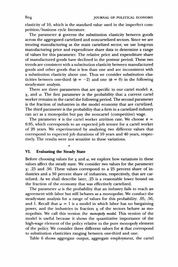
VI. Evaluating the Steady State
Before choosing values for X and w, we explore how variations in these values affect the steady state. We consider two values for the parameter X: .25 and .50. These values correspond to a 25 percent share of in- dustries and a 50 percent share of industries, respectively, that are car- telized. As we shall describe later, .25 is a reasonable lower bound on the fraction of the economy that was effectively cartelized.
The parameter w is the probability that an industry fails to reach an
agreement with labor but still behaves as a monopolist. We conduct the
steady-state analysis for a range of values for this probability: .05, .50, and 1. Recall that o = 1 is a model in which labor has no bargaining power, and the industries in fraction X of the sectors behave as mo-
nopolists. We call this version the monopoly model. This version of the model is useful because it shows the quantitative importance of the
high-wage element of the policy relative to the pure monopoly element of the policy. We consider three different values for 4 that correspond to substitution elasticities ranging between one-third and one.
Table 6 shows aggregate output, aggregate employment, the cartel
804

NEW DEAL POLICIES
TABLE 6 CARTEL MODEL STEADY-STATE VARIABLES RELATIVE TO COMPETITIVE MODEL STEADY-
STATE VARIABLES
Cartel Cartel Fraction of Output Employment Wage Employment Searchers
X =.25
o = 1.00: 0=0 0=-1 4=-2
Xw=.50:
40=0 0=-1
0=-2 0 =.05:
ck=0
0=-2
o = 1.00: 4=0 l= -1 0=-2
CO =.50: 0=0 0= -1
0=-2 o0=.05:
0=0 0=-1 0=-2
.97 .98 .96 .91 .00
.97 .98 .96 .94 .00
.97 .98 .96 .96 .00
.94 .96 1.04 .82 .01
.94 .95 1.04 .87 .01
.95 .95 1.04 .89 .01
.86 .90 1.35 .57 .04
.85 .88 1.34 .67 .05
.86 .87 1.34 .70 .06
X=.50
.94
.94
.93
.89
.89
.89
.76
.75
.75
.96
.96
.96
.92
.92
.91
.81
.79
.78
.93
.93
.93
.98
.98
.98
1.18 1.16 1.15
.91
.93
.94
.82
.86
.87
.58
.65
.67
.00
.00
.00
.02
.02
.02
.09
.11
.11
NOTE.-X is the fraction of industries that are cartelized, w is the probability that a firm in a cartelized industry can act as a monopolist but pay the noncartel wage, and 1/(1 - <4) is the substitution elasticity.
(insider) wage, and employment in the cartel sector divided by their
respective competitive steady-state values. The table also shows the frac- tion of workers searching for a cartel job.
The cartel policy significantly depresses output and employment pro- vided that w is low. For example, with X = .25 and co = .05, output falls 14 percent relative to competition; for X = .50 and w = .05, output falls about 25 percent relative to pure competition. Lower output and em-
ployment are associated with significant increases in the wage in the cartelized sector. For X = .25 and o = .05, the cartelized wage is about 36 percent above its value in the competitive economy; for X = .50 and X = .05, the cartelized wage is about 16 percent.
The key depressing element of the policy is not monopoly per se, but rather the link between wage bargaining and monopoly. To see this, note that the cartelized wage in the monopoly version of the model in which labor has no bargaining power (w = 1) is about the same as the
805
JOURNAL OF POLITICAL ECONOMY
wage in the competitive model. In this case, aggregate output is not much lower than its level in the competitive model. However, fixing the size of the cartelized sector (X), we see that reducing o (raising labor's
bargaining power) raises the wage and consequently reduces em-
ployment. The link between wage bargaining and monopoly is key because rais-
ing the wage above its competitive level in our model requires imperfect competition. In the absence of rents, constant returns to scale and the
competitive rental price of capital imply that the wage rate cannot ex- ceed the marginal product of labor. The fact that labor unions aggres- sively campaigned against antitrust prosecution of firms when New Deal
policies began to shift in the late 1930s empirically supports this mech- anism in our model (see Hawley 1966).
The impact of the policy also depends on the fraction of the economy covered by the policies (X). Fixing the value of w and increasing X reduces output and employment because more of the economy is cartelized.
Note that the policy depresses employment and output in both the cartelized and competitive sectors. The reason is that the decline in intermediate goods output from the cartelized sector reduces the mar-
ginal product of intermediate goods from the competitive sector in the
production of the final good. This decline in the marginal product happens as long as q < 1 (the intermediate goods aggregates from the two sectors are not perfect substitutes in final goods production). Note that the change in aggregate output is almost the same for all three values of q that we consider.
Another indirect effect of the cartelization policy is that the high cartel wage induces some household members to search for high-paying cartel jobs. For example, for X = .25 and o = .05, about 5 percent of individuals involved in market activity search for a cartel job. For X = .5 and w = .05, about 11 percent of workers search for a cartel job. This means that the policy depresses employment more than it depresses labor force participation.
In summary, the steady-state general equilibrium works as follows. The policy raises the wage in the cartel sector, which reduces output in the cartel sector. This decrease in cartel output affects the competitive wage through its impact on the value of the marginal product of labor in the competitive sector. The low competitive wage and the wage gap between the two sectors reduce employment in the competitive sector, since some individuals choose to search for a carteljob and some choose to take leisure rather than work for the low competitive wage. The gap between the steady-state cartelized wage and the competitive wage is determined solely by the policy parameters (X and co), the cartel attrition probability (ir), and the interest rate. Thus search activity has no effect
8o6
on the cartelized wage because the cartel workers control the size of their group.
These results show that a small value of co will be required to under- stand the impact of New Deal policies, because wages were substantially above normal in the cartelized sectors. We now turn to the choice of values for X and X to compute the transition path of the model economy.
VII. Comparing the Model to the Data: 1934-39
We compute the transition path for the purely competitive version and the cartel version of our model from initial conditions in 1934 to their
respective steady states. We then compare the predicted variables from the two models to the data between 1934 and 1939. We choose 1934- 39 because 1934 is the first full year of the policy and the policies began to change significantly after 1939.
We first choose parameter values for X and w. We choose a conservative value for X, which is .32. This is the fraction of the economy covered just by those industries we previously classified as cartelized on the basis of wages, prices, and government reviews: manufacturing, bituminous coal, and petroleum.19
We choose co = .10, which yields a cartelized wage that is 20 percent above its competitive steady-state value. We choose this number because the average manufacturing wage is about 20 percent above trend during the late 1930s, and we assume that the wage would have been near its normal level in the absence of these policies. Given X, this value of o
produces a steady-state cartel wage that is 20 percent above the steady- state wage in the perfectly competitive version of the model. (For the
competitive model, X = 0.) Finally, we choose 4 = -1, which is con- sistent with the long-run declines in the relative price of manufactured goods and in its expenditure share. (Recall that aggregate output is insensitive to the value of this parameter in the range we considered.)
We also need an initial condition for the capital stock in the model. We find that the overall capital stock in 1934 is about 15 percent below trend, which reflects the low level of investment during the Depression. We therefore specify the initial capital stock in each of the two sectors to be 15 percent below the steady state.
Cole and Ohanian (1999) report that measured TFP is significantly below trend in 1933 and recovers back to trend by 1936. We therefore feed into the competitive model the observed sequence of TFP values relative to trend between 1934 and 1936 followed by the steady-state TFP value thereafter. For the cartel model, we have to modify this pro-
19 Manufacturing accounts for 28 percent of output, and the remaining sectors account
for about 4 percent of output in 1929.
807 NEW DEAL POLICIES

JOURNAL OF POLITICAL ECONOMY
cedure because with imperfect competition, measured TFP and the true
technology level differ. We therefore feed in a sequence of TFP values such that measured TFP in the cartel model is the same as that in the data. We then compute the perfect foresight transition path for the two versions of our model.
Figure 2 compares the recovery in output in the models to actual
output during the New Deal. The figure shows that the recovery in the cartel model is much closer to the actual recovery. Tables 7 and 8 present details for the two models.
Table 7 presents the results for the competitive model. The predicted recovery from this model differs significantly from the actual 1934-39
recovery. Predicted economic activity is too high, and the predicted wage is much lower than the wage in manufacturing. In particular, predicted output returns nearly to trend by 1936, whereas actual output remains about 25 percent below trend. Predicted labor rises above trend by 1936. In contrast, actual labor input remains about 25 percent below trend
through the period. Predicted consumption recovers nearly to trend by the end of the decade. Actual consumption remains about 25 percent below trend. There is an even larger disparity between predicted and actual investment. Predicted investment rises 18 percent above trend
by 1936 because of the low initial capital stock and the rapid recovery of productivity. In contrast, actual investment recovers only to 50 percent of its trend level. The predicted wage is initially low and then rises nearly to trend as TFP rises and the capital stock grows. In contrast, the man-
ufacturing wage is considerably above trend over the 1934-39 period. The predicted equilibrium path from the competitive model differs
considerably from the actual path of the U.S. economy. It is natural to suspect that slowing down the convergence of the
competitive model would let it match the actual recovery much better. Cole and Ohanian (1999) showed that this was not the case. We found that plausibly parameterized "slow converging" versions of the compet- itive model have the same problem as the standard model by predicting that the economy should have been near trend by 1939 and that the
wage should have been below normal during the recovery. We now turn to the cartel model. To compute the equilibrium path
of this model, we need a value for one additional state variable, which is the initial number of insiders in the cartelized sector. We choose this number by dividing trend-adjusted 1933 manufacturing employment by its 1929 value, which yields .58.
Table 8 shows output, consumption, investment, employment, search- ers divided by the sum of workers and searchers, employment in the cartel sector, employment in the competitive sector, the wage in the cartel sector, and the wage in the competitive sector.
The table shows that the equilibrium path of the cartel model is similar
808
100 p , , _ _ , m m - m m mm m m - m , _ _ -
90O ' Competitive Model
PS 90 m- -m'
S - - , Cartel Model ?. O^ 80 , _ '
O-mr 70
60
i 60
50 , -,,
1934 1935 1936 1937 1938 1939
Year
FIG. 2.-Output in the data and in the models
JOURNAL OF POLITICAL ECONOMY
TABLE 7 EQUILIBRIUM PATH FROM THE COMPETITIVE MODEL
Output Consumption Investment Employment Wage
1934 .87 .90 .73 .98 .89 1935 .92 .91 .97 1.01 .91 1936 .97 .93 1.18 1.03 .94 1937 .98 .94 1.14 1.03 .95 1938 .98 .95 1.12 1.02 .96 1939 .99 .96 1.09 1.02 .97
to the actual path of the economy and sheds light on a number of the
puzzles about the weak recovery. Two key puzzles in the data are the low levels of output and labor input. These variables rise from their
trough levels between 1934 and 1936 and are flat afterward in the data, remaining about 20-25 percent below trend. The cartel model predicts very similar patterns for these variables. They rise between 1934 and 1936 and are flat afterward. The cartel model economy remains signif- icantly depressed in 1939, though the severity of the depression is less than in the data. Output in the model is 13 percent below its competitive steady-state level, and employment is 11 percent below its steady-state level. The model also captures the pattern of consumption. Actual con-
sumption is flat throughout the recovery, remaining about 25 percent below trend. The pattern of consumption in the cartel model is also flat, rising from 16 percent below its competitive steady-state level in 1934 to 14 percent below in 1939. The cartel model predicts a much
stronger investment recovery: an increase from about 60 percent below its competitive steady-state level in 1934 to 13 percent below in 1939. While this deviation between theory and data is significant, it is much smaller than the deviation between investment in the competitive model and in the data. Investment in the competitive model is 18 percent above its competitive steady-state level in 1936. This stands in contrast to in- vestment in the cartel model, which is 12 percent below the competitive steady-state level.
We now discuss some other features of the data and the corresponding predictions of the model. The manufacturing wage, which we take to be a cartelized wage in the data, rises from 11 percent above trend in 1934 to about 20 percent above trend at the end of the decade. The cartelized wage in the model exhibits a similar increase. It rises from about 15 percent above its competitive steady-state level in 1934 to 20 percent by 1939. While the parameter w was chosen so that the steady- state wage is 20 percent above the competitive steady-state level, this choice places no restrictions on the time path of the cartelized wage as it converges to its steady-state value. Thus the model reproduces the time path in the cartel wage over the recovery period.
81i

TABLE 8 EQUILIBRIUM PATH FROM THE CARTEL MODEL
EMPLOYMENT WAGE
Cartel Competitive Cartel Competitive OUTPUT CONSUMPTION INVESTMENT EMPLOYMENT SEARCHERS* Sector Sector Sector Sector
1934 .77 .85 .40 .82 .07 .68 .89 1.16 .81 1935 .81 .85 .62 .84 .11 .69 .92 1.19 .83 1936 .86 .85 .87 .89 .06 .72 .97 1.20 .83 1937 .87 .86 .90 .90 .04 .73 .98 1.20 .83 1938 .86 .86 .86 .89 .06 .72 .97 1.20 .84 1939 .87 .86 .88 .89 .04 .73 .97 1.20 .84
* Searchers divided by the sum of workers and searchers.
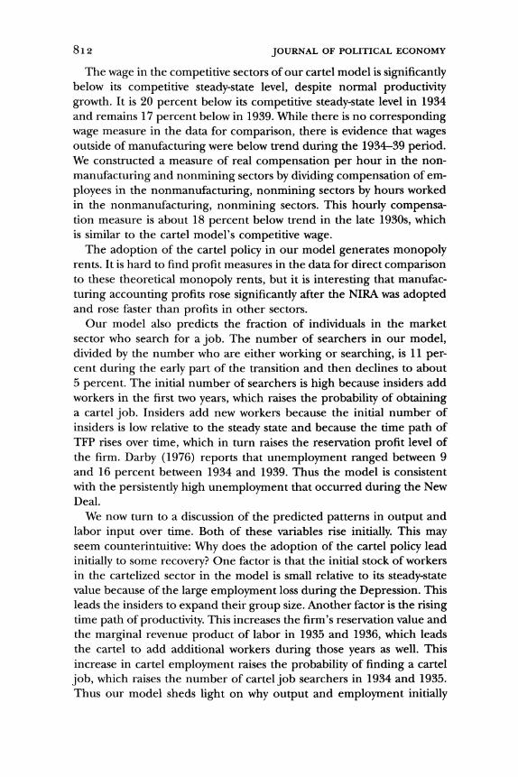
JOURNAL OF POLITICAL ECONOMY
The wage in the competitive sectors of our cartel model is significantly below its competitive steady-state level, despite normal productivity growth. It is 20 percent below its competitive steady-state level in 1934 and remains 17 percent below in 1939. While there is no corresponding wage measure in the data for comparison, there is evidence that wages outside of manufacturing were below trend during the 1934-39 period. We constructed a measure of real compensation per hour in the non-
manufacturing and nonmining sectors by dividing compensation of em-
ployees in the nonmanufacturing, nonmining sectors by hours worked in the nonmanufacturing, nonmining sectors. This hourly compensa- tion measure is about 18 percent below trend in the late 1930s, which is similar to the cartel model's competitive wage.
The adoption of the cartel policy in our model generates monopoly rents. It is hard to find profit measures in the data for direct comparison to these theoretical monopoly rents, but it is interesting that manufac-
turing accounting profits rose significantly after the NIRA was adopted and rose faster than profits in other sectors.
Our model also predicts the fraction of individuals in the market sector who search for a job. The number of searchers in our model, divided by the number who are either working or searching, is 11 per- cent during the early part of the transition and then declines to about 5 percent. The initial number of searchers is high because insiders add workers in the first two years, which raises the probability of obtaining a cartel job. Insiders add new workers because the initial number of insiders is low relative to the steady state and because the time path of TFP rises over time, which in turn raises the reservation profit level of the firm. Darby (1976) reports that unemployment ranged between 9 and 16 percent between 1934 and 1939. Thus the model is consistent with the persistently high unemployment that occurred during the New Deal.
We now turn to a discussion of the predicted patterns in output and labor input over time. Both of these variables rise initially. This may seem counterintuitive: Why does the adoption of the cartel policy lead
initially to some recovery? One factor is that the initial stock of workers in the cartelized sector in the model is small relative to its steady-state value because of the large employment loss during the Depression. This leads the insiders to expand their group size. Another factor is the rising time path of productivity. This increases the firm's reservation value and the marginal revenue product of labor in 1935 and 1936, which leads the cartel to add additional workers during those years as well. This increase in cartel employment raises the probability of finding a cartel
job, which raises the number of cartel job searchers in 1934 and 1935. Thus our model sheds light on why output and employment initially
812
expanded during the New Deal and why that initial recovery stalled by the late 1930s.
VIII. Conclusion
New Deal labor and industrial policies did not lift the economy out of the Depression as President Roosevelt had hoped. Instead, the joint policies of increasing labor's bargaining power and linking collusion with paying high wages prevented a normal recovery by creating rents and an inefficient insider-outsider friction that raised wages significantly and restricted employment.
Not only did the adoption of these industrial and trade policies co- incide with the persistence of depression through the late 1930s, but the subsequent abandonment of these policies coincided with the strong economic recovery of the 1940s. Further research should evaluate the contribution of this policy shift to the World War II economic boom.
Appendix
A. Deriving the Insider's Maximization Problem
We derive (9). Start by taking as given the sequence of offers {fw,, nj and note that the present value of lifetime earnings of the insiders (workers in the cartel at the beginning of the period), under the assumption that they work in the competitive sector if they leave the cartel, is implicitly given by
ntyW = min [n,, n,] w, + max [0, n,- n-]Xt
+ Q' {irmin [nt, n,]W,+ + (1 - r) min [n,, n,]lOX,+}),
where W denotes the present value of lifetime earnings to an insider in period t, and X, denotes the present value of lifetime earnings to a worker in a com- petitive industry, where
X, = wf+ Q ,+t t+
In the period t flow payoff, min [nt, nt] is the number of insiders who continue working in the industry this period and max [0, n, - n, is the number who are laid off and work in a competitive industry. The future payoff to those who are not laid off in period t accounts for the fact that between periods the fraction 1 - 7r of the cartel workers (insiders who work that period plus new members added to the cartel) will suffer attrition. Since W,- X, = V(n,), we obtain (9).
If n, > n,, the current surplus received by cartel workers is n,(w, - w,). However, only the portion n,(, - w,) is received by the period t insiders. Similarly, the present value of surplus received by insiders at the beginning of period t + 1, n,,+[Wt+l
- V(nt+l)], includes the present value of surplus received by both the
period t insiders, whose number is 7min [nt, nt], and the new hires in period t, whose number is 7rmax [0, nt- n,].
813 NEW DEAL POLICIES
JOURNAL OF POLITICAL ECONOMY
B. Proof of Proposition 1
Part i is proved by contradiction. If IIt(w, n) > P, then the workers could raise w, keeping n the same, and thereby raise the value of the objective function.
Part ii is proved by contradiction. Assume that n, < n,, and note that when we set nt = n, and keep n,,, unchanged, the workers' current return is higher and their expected future is unchanged. To see that their current payoff is higher, note that wt is higher (given that it is set according to part i), and they receive this return with probability one. To see that their expected future return is unchanged, note first that the likelihood that an initial worker in period t remained employed in period t+ 1 was (nJ/n,)min (n,+ l/rnt, 1). Under the proposed deviation, there are no layoffs in period t, but the higher layoffs in period t+ 1 just offset this and the probability of working in period t + 1 for an initial worker in period t is unchanged by construction. Hence, their future payoff is unchanged, since the payoff per worker who is employed in period t + 1 is unchanged. If nt+l is chosen optimally given that the number of initial workers in period t + 1 is irn,, the future payoff could be even higher: since Vt+,(rnt) is optimal, V,(+(irnt) > (nin,)V,+l(,n,).
Part iii is proved by contradiction. As in the proof of part ii, consider deviating and setting employment to n, and the wage according to part i. Since the total profits earned by the workers are II,(0, n) - t in period t, we need only show that
H,(O, nt) - Pt- ntwt + 7rQ+ min 1 nt+l _ WVt+2(nt+,) H4O- -iz-) m-+ i+ (mi -W - n +, V +2(7rn+1) > n, Qt 7 an,\ Qt+1
II(0,.. hni,) -Pt,_-_n w+l_wQl ++.[.t+ 2 \+ (7n)' n ~+1m - -min 1, Wt +i - Wt+1 + r V- 2(n+1) n, nt Qt ' 'n, t \Q+1
(Al)
Note that
min[1,- n
(min[, a +]/ nt n, rntJ
and therefore the second terms are equal in the two expressions by construction. Hence we need only show that
t,(O, n,) - Pt- n ,twt (0, n t) - Pt-nw (A2)
n, nt
which follows trivially from the fact that n,< N(w,), and the profit function nIt(wt, n,) is concave in n,.
The proof of part iv is similar to that of part iii. We again need to show that (Al) is satisfied, and this follows trivially from the assumption that n, > N1(wt).
C. Proof of Proposition 2
The proof follows trivially from the fact that wt is the maximal wage rate in period t and that therefore the value of (9) is bounded above by
t= irQt(wt* - w,) and this sequence achieves that bound. The uniqueness of the sequence follows from the fact that I is strictly decreasing in w.
814
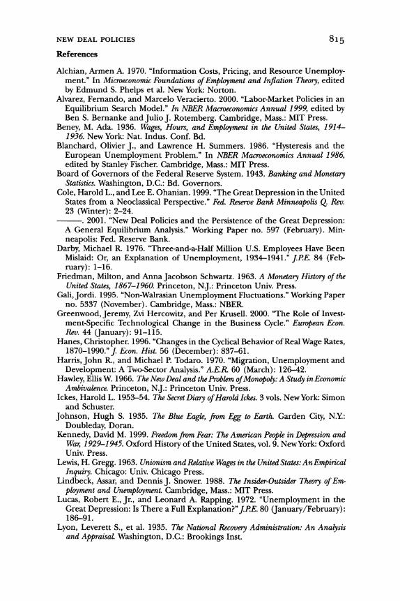
References
Alchian, Armen A. 1970. "Information Costs, Pricing, and Resource Unemploy- ment." In Microeconomic Foundations of Employment and Inflation Theory, edited by Edmund S. Phelps et al. New York: Norton.
Alvarez, Fernando, and Marcelo Veracierto. 2000. "Labor-Market Policies in an Equilibrium Search Model." In NBER Macroeconomics Annual 1999, edited by Ben S. Bernanke and Julio J. Rotemberg. Cambridge, Mass.: MIT Press.
Beney, M. Ada. 1936. Wages, Hours, and Employment in the United States, 1914- 1936. New York: Nat. Indus. Conf. Bd.
Blanchard, Olivier J., and Lawrence H. Summers. 1986. "Hysteresis and the European Unemployment Problem." In NBER Macroeconomics Annual 1986, edited by Stanley Fischer. Cambridge, Mass.: MIT Press.
Board of Governors of the Federal Reserve System. 1943. Banking and Monetary Statistics. Washington, D.C.: Bd. Governors.
Cole, Harold L., and Lee E. Ohanian. 1999. "The Great Depression in the United States from a Neoclassical Perspective." Fed. Reserve Bank Minneapolis Q. Rev. 23 (Winter): 2-24.
. 2001. "New Deal Policies and the Persistence of the Great Depression: A General Equilibrium Analysis." Working Paper no. 597 (February). Min- neapolis: Fed. Reserve Bank.
Darby, Michael R. 1976. "Three-and-a-Half Million U.S. Employees Have Been Mislaid: Or, an Explanation of Unemployment, 1934-1941." J.PE. 84 (Feb- ruary): 1-16.
Friedman, Milton, and AnnaJacobson Schwartz. 1963. A Monetary History of the United States, 1867-1960. Princeton, NJ.: Princeton Univ. Press.
Gali,Jordi. 1995. "Non-Walrasian Unemployment Fluctuations." Working Paper no. 5337 (November). Cambridge, Mass.: NBER.
Greenwood, Jeremy, Zvi Hercowitz, and Per Krusell. 2000. "The Role of Invest- ment-Specific Technological Change in the Business Cycle." European Econ. Rev. 44 (January): 91-115.
Hanes, Christopher. 1996. "Changes in the Cyclical Behavior of Real Wage Rates, 1870-1990."J. Econ. Hist. 56 (December): 837-61.
Harris, John R., and Michael P. Todaro. 1970. "Migration, Unemployment and Development: A Two-Sector Analysis." A.E.R 60 (March): 126-42.
Hawley, Ellis W. 1966. The New Deal and the Problem of Monopoly: A Study in Economic Ambivalence. Princeton, N.J.: Princeton Univ. Press.
Ickes, Harold L. 1953-54. The Secret Diary of Harold Ickes. 3 vols. New York: Simon and Schuster.
Johnson, Hugh S. 1935. The Blue Eagle, from Egg to Earth. Garden City, N.Y.: Doubleday, Doran.
Kennedy, David M. 1999. Freedom from Fear: The American People in Depression and War, 1929-1945. Oxford History of the United States, vol. 9. NewYork: Oxford Univ. Press.
Lewis, H. Gregg. 1963. Unionism and Relative Wages in the United States: An Empirical Inquiry. Chicago: Univ. Chicago Press.
Lindbeck, Assar, and Dennis J. Snower. 1988. The Insider-Outsider Theory of Em- ployment and Unemployment. Cambridge, Mass.: MIT Press.
Lucas, Robert E., Jr., and Leonard A. Rapping. 1972. "Unemployment in the Great Depression: Is There a Full Explanation?"J.PE. 80 (January/February): 186-91.
Lyon, Leverett S., et al. 1935. The National Recovery Administration: An Analysis and Appraisal. Washington, D.C.: Brookings Inst.
815 NEW DEAL POLICIES
816 JOURNAL OF POLITICAL ECONOMY
Millis, Harry, and Emily Clark Brown. 1950. From the Wagner Act to Taft-Hartley: A Study of National Labor Policy and Labor Relations. Chicago: Univ. Chicago Press.
Mulligan, Casey B. 2000. "A Century of Labor-Leisure Distortions." Working Paper no. 8774 (February). Cambridge, Mass.: NBER.
National Recovery Administration. 1933-35. Codes of Fair Competition. 23 vols. Washington, D.C.: Government Printing Office.
National Review Recovery Board. 1935. Reports to the President of the United States. Washington, D.C.: Government Printing Office.
Pierce, Phyllis, ed. 1982. The DowJones Averages, 1885-1980. Homewood, Ill.: Dow Jones-Irwin.
Posner, Richard A. 1970. "A Statistical Study of Antitrust Enforcement." J. Law and Econ. 13 (October): 365-419.
Reynolds, Lloyd G., and Cynthia H. Taft. 1955. The Evolution of Wage Structure. New Haven, Conn.: Yale Univ. Press.
Ross, Arthur M. 1948. Trade Union Wage Policy. Berkeley: Univ. California Press. Taft, Philip. 1964. Organized Labor in American History. New York: Harper and
Row.


![Cap-and-Trade Spells Economic Disaster for …CAP-AND-TRADE rights and market incentives" to lessen pollution.1 2 Emissions, those economists argue, [could be reduced] by assigning](https://img.pdfslide.us/doc/110x75/5fb9f296fbcd5d37b25e7609/cap-and-trade-spells-economic-disaster-for-cap-and-trade-rights-and-market-incentives.jpg)