Embed Size (px)
Citation preview

Article
Neurons in Macaque Area
V4 Are Tuned for ComplexSpatio-Temporal PatternsHighlights
d V4 neurons show complex spatio-temporal tuning dynamics
d Neurons with heterogeneous shape selectivity have diverse
temporal response kernels
d Population shape decoding models benefit from this
temporal information
d Temporal information could provide a multiplexed code for
spatio-temporal features
Nandy et al., 2016, Neuron 91, 1–11August 17, 2016 ª 2016 Elsevier Inc.http://dx.doi.org/10.1016/j.neuron.2016.07.026
Authors
Anirvan S. Nandy, Jude F. Mitchell,
Monika P. Jadi, John H. Reynolds
In Brief
Neurons in area V4 play a critical role in
object recognition. Here, Nandy et al.
show that V4 neurons exhibit variation in
their temporal response profiles across
spatial locations, suggesting a
multiplexed code for spatio-temporal
features.
Please cite this article in press as: Nandy et al., Neurons in Macaque Area V4 Are Tuned for Complex Spatio-Temporal Patterns, Neuron (2016), http://dx.doi.org/10.1016/j.neuron.2016.07.026
Neuron
Article
Neurons in Macaque Area V4 Are Tunedfor Complex Spatio-Temporal PatternsAnirvan S. Nandy,1,* Jude F. Mitchell,1,3 Monika P. Jadi,2 and John H. Reynolds11Systems Neurobiology Laboratories, The Salk Institute for Biological Studies, La Jolla, CA 92037, USA2Computational Neurobiology Laboratories, The Salk Institute for Biological Studies, La Jolla, CA 92037, USA3Present address: Department of Brain & Cognitive Sciences, University of Rochester, Rochester, NY 14627, USA*Correspondence: [email protected]
http://dx.doi.org/10.1016/j.neuron.2016.07.026
SUMMARY
To deepen our understanding of object recognition, itis critical to understand the nature of transformationsthat occur in intermediate stages of processing in theventral visual pathway, such as area V4. Neurons inV4 are selective to local features of global shape,such as extended contours. Previously, we foundthat V4 neurons selective for curved elements exhibita high degree of spatial variation in their preference.If spatial variation in curvature selectivity was alsomarked by distinct temporal response patterns atdifferent spatial locations, then it might be possibleto untangle this information in subsequent process-ing based on temporal responses. Indeed, we findthat V4 neurons whose receptive fields exhibit intri-cate selectivity also show variation in their temporalresponses across locations. A computational modelthat decodes stimulus identity based on populationresponses benefits from using this temporal informa-tion, suggesting that it could provide a multiplexedcode for spatio-temporal features.
INTRODUCTION
Visual information impingingon thephotoreceptors in the retina is
initially processed in the retinal circuit (Field and Chichilnisky,
2007) before being relayed via the lateral geniculate nucleus
(LGN) on to the primary visual cortex. Processing of visual shape
continues downstream in a set of cortical areas in the ventral
cortical pathway in the temporal lobe (DiCarlo et al., 2012). At
the earliest stages of visual processing in the retina, systems
identification techniques, such as reverse correlation, have
spurred progress for understanding of how visual inputs are
pooled to give rise to the receptive fields (RFs) of visual neurons
(Field et al., 2010; Schwartz et al., 2012). Similar approaches
have provided key insights about the population RFs of LGN af-
ferents that make monosynaptic connections to neurons in the
primary visual cortex (V1) (Jin et al., 2011) and the detailed spatial
structure of RFs in the secondary visual cortex (V2) (Anzai et al.,
2007; Tao et al., 2012). At later stages of processing along the
ventral stream it has been much more difficult to constrain such
mechanistic models of receptive field structure. However, there
has been considerable progress toward understanding what in-
formation is encoded based on decoding population responses
(Pasupathy and Connor, 2002; Rust and Dicarlo, 2010). Area V4
lies at a critical intermediate juncture in the transformations that
occur between V1/V2 and the final stages of shape processing
in the inferotemporal cortex (areas TEO and TE). Earlier studies
in V4 found that many neurons were selective to extended con-
tours that form curved shapes (Pasupathy and Connor, 2001,
1999). A detailed understanding of RF organization in V4 remains
crucial for understanding the more invariant forms of object
recognition that then follow in inferotemporal cortex.
In a recent study (Nandy et al., 2013), we examined the fine
spatial structure of V4 RFs using reverse correlation techniques
to estimate the tuning for curvature. We found that V4 neurons
exhibit a tradeoff between curvature selectivity and spatial
invariance. Neurons tuned to curved shapes exhibited very
limited spatial invariance, while those that preferred straight con-
tours tended to show spatially invariant tuning. This diversity was
explained by the fine-scale RF structure: fine-scale maps of
orientation tuning across the RF for neurons preferring curved
contours showed heterogeneous local variation, whereas tuning
was homogeneous and thus translation invariant for neurons
preferring straight contours.
This previous analysis examined a temporally averaged static
picture of the RF structure. Here we investigate whether the
homogeneity/heterogeneity observed in the spatial domain
extended to the temporal domain as well. We find that the fine-
scale RFs in V4 often show previously unappreciated spatio-
temporal structure. Some neurons have progressively shifting
spatial kernels. Others show distinct temporal signatures in
different RF sub-regions, while others have spatial kernels that
dissipate over time from the center to the edges.
As in the spatial domain, the complexity of these temporal pat-
terns varied with the heterogeneity of the fine-scale receptive
field map: neurons with spatially varying shape tuning have
distinct temporal response patterns that unfold across RF loca-
tions. In contrast, neurons with spatially invariant shape tuning
have similar temporal response patterns across RF locations.
We find that computational models that use this temporal infor-
mation to decode stimulus identity far outperform simpler
models based on time-averaged spike counts. We suggest
that this tradeoff between simple/complex shape selectivity
and homogeneity/heterogeneity in both the spatial and temporal
domains could potentially reflect a spatio-temporal shape code
in area V4.
Neuron 91, 1–11, August 17, 2016 ª 2016 Elsevier Inc. 1
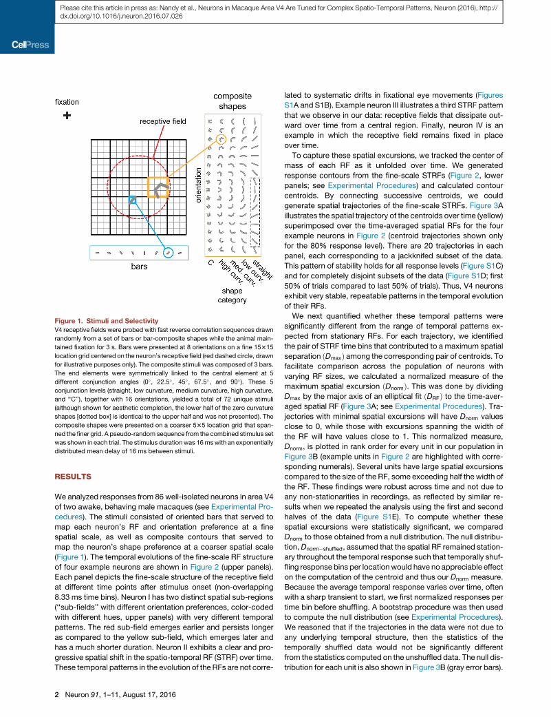
Figure 1. Stimuli and Selectivity
V4 receptive fields were probed with fast reverse correlation sequences drawn
randomly from a set of bars or bar-composite shapes while the animal main-
tained fixation for 3 s. Bars were presented at 8 orientations on a fine 15315
location grid centered on the neuron’s receptive field (red dashed circle, drawn
for illustrative purposes only). The composite stimuli was composed of 3 bars.
The end elements were symmetrically linked to the central element at 5
different conjunction angles (0�, 22.5�, 45�, 67.5�, and 90�). These 5
conjunction levels (straight, low curvature, medium curvature, high curvature,
and ‘‘C’’), together with 16 orientations, yielded a total of 72 unique stimuli
(although shown for aesthetic completion, the lower half of the zero curvature
shapes [dotted box] is identical to the upper half and was not presented). The
composite shapes were presented on a coarser 535 location grid that span-
ned the finer grid. A pseudo-random sequence from the combined stimulus set
was shown in each trial. The stimulus duration was 16mswith an exponentially
distributed mean delay of 16 ms between stimuli.
Please cite this article in press as: Nandy et al., Neurons in Macaque Area V4 Are Tuned for Complex Spatio-Temporal Patterns, Neuron (2016), http://dx.doi.org/10.1016/j.neuron.2016.07.026
RESULTS
We analyzed responses from 86 well-isolated neurons in area V4
of two awake, behaving male macaques (see Experimental Pro-
cedures). The stimuli consisted of oriented bars that served to
map each neuron’s RF and orientation preference at a fine
spatial scale, as well as composite contours that served to
map the neuron’s shape preference at a coarser spatial scale
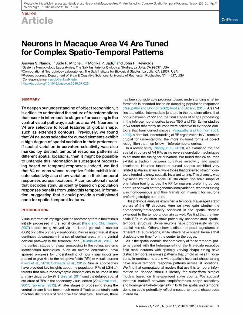
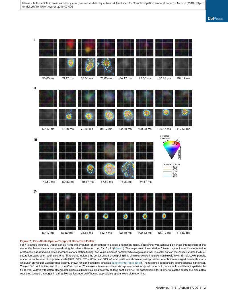
(Figure 1). The temporal evolutions of the fine-scale RF structure
of four example neurons are shown in Figure 2 (upper panels).
Each panel depicts the fine-scale structure of the receptive field
at different time points after stimulus onset (non-overlapping
8.33 ms time bins). Neuron I has two distinct spatial sub-regions
(‘‘sub-fields’’ with different orientation preferences, color-coded
with different hues, upper panels) with very different temporal
patterns. The red sub-field emerges earlier and persists longer
as compared to the yellow sub-field, which emerges later and
has a much shorter duration. Neuron II exhibits a clear and pro-
gressive spatial shift in the spatio-temporal RF (STRF) over time.
These temporal patterns in the evolution of the RFs are not corre-
2 Neuron 91, 1–11, August 17, 2016
lated to systematic drifts in fixational eye movements (Figures
S1A and S1B). Example neuron III illustrates a third STRF pattern
that we observe in our data: receptive fields that dissipate out-
ward over time from a central region. Finally, neuron IV is an
example in which the receptive field remains fixed in place
over time.
To capture these spatial excursions, we tracked the center of
mass of each RF as it unfolded over time. We generated
response contours from the fine-scale STRFs (Figure 2, lower
panels; see Experimental Procedures) and calculated contour
centroids. By connecting successive centroids, we could
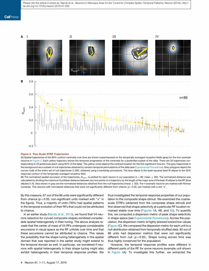
generate spatial trajectories of the fine-scale STRFs. Figure 3A
illustrates the spatial trajectory of the centroids over time (yellow)
superimposed over the time-averaged spatial RFs for the four
example neurons in Figure 2 (centroid trajectories shown only
for the 80% response level). There are 20 trajectories in each
panel, each corresponding to a jackknifed subset of the data.
This pattern of stability holds for all response levels (Figure S1C)
and for completely disjoint subsets of the data (Figure S1D; first
50% of trials compared to last 50% of trials). Thus, V4 neurons
exhibit very stable, repeatable patterns in the temporal evolution
of their RFs.
We next quantified whether these temporal patterns were
significantly different from the range of temporal patterns ex-
pected from stationary RFs. For each trajectory, we identified
the pair of STRF time bins that contributed to a maximum spatial
separation ðDmaxÞ among the corresponding pair of centroids. To
facilitate comparison across the population of neurons with
varying RF sizes, we calculated a normalized measure of the
maximum spatial excursion ðDnormÞ. This was done by dividing
Dmax by the major axis of an elliptical fit ðDRFÞ to the time-aver-
aged spatial RF (Figure 3A; see Experimental Procedures). Tra-
jectories with minimal spatial excursions will have Dnorm values
close to 0, while those with excursions spanning the width of
the RF will have values close to 1. This normalized measure,
Dnorm, is plotted in rank order for every unit in our population in
Figure 3B (example units in Figure 2 are highlighted with corre-
sponding numerals). Several units have large spatial excursions
compared to the size of the RF, some exceeding half the width of
the RF. These findings were robust across time and not due to
any non-stationarities in recordings, as reflected by similar re-
sults when we repeated the analysis using the first and second
halves of the data (Figure S1E). To compute whether these
spatial excursions were statistically significant, we compared
Dnorm to those obtained from a null distribution. The null distribu-
tion,Dnorm�shuffled, assumed that the spatial RF remained station-
ary throughout the temporal response such that temporally shuf-
fling response bins per location would have no appreciable effect
on the computation of the centroid and thus our Dnorm measure.
Because the average temporal response varies over time, often
with a sharp transient to start, we first normalized responses per
time bin before shuffling. A bootstrap procedure was then used
to compute the null distribution (see Experimental Procedures).
We reasoned that if the trajectories in the data were not due to
any underlying temporal structure, then the statistics of the
temporally shuffled data would not be significantly different
from the statistics computed on the unshuffled data. The null dis-
tribution for each unit is also shown in Figure 3B (gray error bars).
preferred orientation
resp
onse
tuning
width
I
II
III
IV
59.17 ms 67.50 ms 75.83 ms 84.17 ms 92.50 ms 100.83 ms 109.17 ms 117.50 ms
50.83 ms 59.17 ms 67.50 ms 75.83 ms 84.17 ms 92.50 ms 100.83 ms 109.17 ms
42.50 ms 50.83 ms 59.17 ms 67.50 ms 75.83 ms 84.17 ms
59.17 ms 67.50 ms 75.83 ms 84.17 ms 92.50 ms 100.83 ms 109.17 ms 117.50 ms
90%80%70%60%50%
reponse contours
Figure 2. Fine-Scale Spatio-Temporal Receptive Fields
For 4 example neurons. Upper panels, temporal evolution of smoothed fine-scale orientation maps. Smoothing was achieved by linear interpolation of the
respective fine-scale maps obtained using the oriented bars on the 15315 grid (Figure 1). The maps are color-coded as follows: hue indicates local orientation
preference, saturation indicates sharpness of orientation tuning, and value indicates normalized average response. The color cone in the inset illustrates the hue-
saturation-value color-coding scheme. Time points indicate the center of non-overlapping time bins relative to stimulus onset (bin width = 8.33ms). Lower panels,
response contours at 5 response levels (90%, 80%, 70%, 60%, and 50% of local peak) are shown superimposed on orientation-averaged fine-scale maps
(shown in grayscale). Contour lines are only shown for significant time bins (see Experimental Procedures). The response contours are color coded as in the inset.
The red ‘‘+’’ depicts the centroid of the 90% contour. The 4 example neurons illustrate representative temporal patterns in our data: I has different spatial sub-
fields (red, yellow) with different temporal dynamics; II shows a progressively shifting spatial kernel; the spatial kernel for III emerges at the center and dissipates
over time toward the edges in a ring-like fashion; neuron IV has no appreciable spatial excursion over time.
Neuron 91, 1–11, August 17, 2016 3
Please cite this article in press as: Nandy et al., Neurons in Macaque Area V4 Are Tuned for Complex Spatio-Temporal Patterns, Neuron (2016), http://dx.doi.org/10.1016/j.neuron.2016.07.026
I II III IVA
B
DRF
DmaxDnorm=
Dno
rm
II
I
III
IV
n=86
-0.2
0
0.2
0.4
0.6
0.8
Figure 3. Fine-Scale STRF Trajectories
(A) Spatial trajectories of the 80% contour centroids over time are shown superimposed on the temporally averaged receptive fields (gray) for the four example
neurons in Figure 2. Each yellow trajectory shows the temporal progression of the centroids for a jackknifed subset of the data. There are 20 trajectories cor-
responding to 20 jackknives (each using 95% of the data). The yellow circle depicts the centroid location for the first significant time bin. The gray trajectories in
the background are a subset of null trajectories obtained by random temporal permutations of the data (see Experimental Procedures). Gray polygons depict the
convex hulls of the entire set of null trajectories (1,000, obtained using a bootstrap procedure). The blue ellipse is the least-squares best-fit ellipse to the 50%
response contour of the temporally averaged receptive field.
(B) The normalized spatial excursion of the trajectories, Dnorm, is plotted for each neuron in our population (n = 86; mean ± SD). The normalized distance was
calculated by dividing themaximum Euclidean distance between any two points on a trajectory by the length of the major axis of the best-fit ellipse to the RF (blue
ellipses in A). Also shown in gray are the normalized distances obtained from the null trajectories (mean ± SD). The 4 example neurons are marked with Roman
numerals. The neurons with normalized distances that were not significantly different from chance ðp= 0:05Þ are marked with a red ‘‘x’’.
Please cite this article in press as: Nandy et al., Neurons in Macaque Area V4 Are Tuned for Complex Spatio-Temporal Patterns, Neuron (2016), http://dx.doi.org/10.1016/j.neuron.2016.07.026
By this measure, 67 out of the 86 units were significantly different
from chance (p< 0:05; non-significant units marked with ‘‘x’’ in
the figure). Thus, a majority of units (78%) had spatial patterns
in the temporal evolution of their RFs that could not be attributed
to chance.
In an earlier study (Nandy et al., 2013), we found that V4 neu-
rons selective for curved composite shapes exhibited consider-
able spatial heterogeneity in their tuning. The above analysis re-
veals that the center of mass of V4 RFs undergoes considerable
excursions in visual space as the RF unfolds over time and that
these excursions cannot be attributed to chance. This raises
the possibility that the shape tuning heterogeneity in the spatial
domain that was reported in the earlier study might extend to
the temporal domain as well. In particular, we wondered if neu-
rons with spatial heterogeneity in their shape tuning might also
exhibit heterogeneity in their temporal response profiles. We
4 Neuron 91, 1–11, August 17, 2016
thus investigated the temporal response properties of our popu-
lation to the composite shape stimuli. We examined the coarse-
scale STRFs (obtained from the composite shape stimuli) and
first observed that shape selectivity at a particular RF location re-
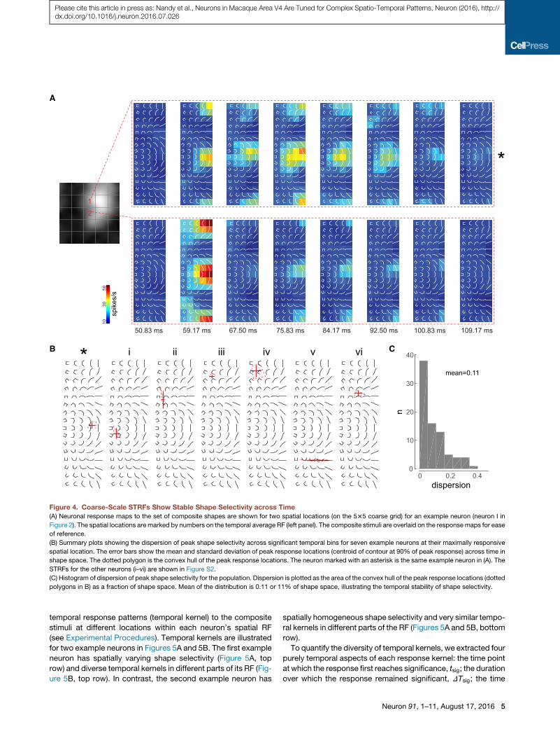
mained stable over time (Figures 4A, 4B, and S2). To quantify
this, we computed a dispersion metric of peak shape selectivity
in shape space (see Experimental Procedures). Across the pop-
ulation, the dispersion metric is highly skewed toward low values
(Figure 4C).We compared the dispersionmetric for each unit to a
null distribution obtained from temporally shuffled data. 82 out of
86 units had dispersion metrics that were not significantly
different from null ðp> 0:05Þ. Shape tuning across time was
thus highly conserved for the population.
However, the temporal response profiles were different in
different parts of the RF for some neurons (example unit shown
in Figure 4A). To investigate this further, we extracted the
1
2
50.83 ms 59.17 ms 67.50 ms 75.83 ms 84.17 ms 92.50 ms 100.83 ms 109.17 ms
spik
es/s
1030
50A
B C
*
* i ii iii iv v vi
0.20 0.40
10
20
30
40
dispersion
n
mean=0.11
Figure 4. Coarse-Scale STRFs Show Stable Shape Selectivity across Time
(A) Neuronal response maps to the set of composite shapes are shown for two spatial locations (on the 535 coarse grid) for an example neuron (neuron I in
Figure 2). The spatial locations are marked by numbers on the temporal average RF (left panel). The composite stimuli are overlaid on the response maps for ease
of reference.
(B) Summary plots showing the dispersion of peak shape selectivity across significant temporal bins for seven example neurons at their maximally responsive
spatial location. The error bars show the mean and standard deviation of peak response locations (centroid of contour at 90% of peak response) across time in
shape space. The dotted polygon is the convex hull of the peak response locations. The neuron marked with an asterisk is the same example neuron in (A). The
STRFs for the other neurons (i–vi) are shown in Figure S2.
(C) Histogram of dispersion of peak shape selectivity for the population. Dispersion is plotted as the area of the convex hull of the peak response locations (dotted
polygons in B) as a fraction of shape space. Mean of the distribution is 0.11 or 11% of shape space, illustrating the temporal stability of shape selectivity.
Please cite this article in press as: Nandy et al., Neurons in Macaque Area V4 Are Tuned for Complex Spatio-Temporal Patterns, Neuron (2016), http://dx.doi.org/10.1016/j.neuron.2016.07.026
temporal response patterns (temporal kernel) to the composite
stimuli at different locations within each neuron’s spatial RF
(see Experimental Procedures). Temporal kernels are illustrated
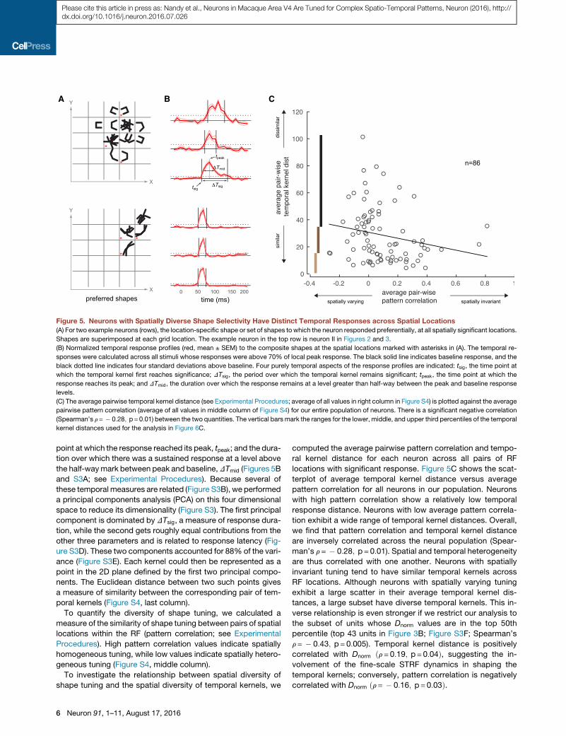
for two example neurons in Figures 5A and 5B. The first example
neuron has spatially varying shape selectivity (Figure 5A, top
row) and diverse temporal kernels in different parts of its RF (Fig-
ure 5B, top row). In contrast, the second example neuron has
spatially homogeneous shape selectivity and very similar tempo-
ral kernels in different parts of the RF (Figures 5A and 5B, bottom
row).
To quantify the diversity of temporal kernels, we extracted four
purely temporal aspects of each response kernel: the time point
at which the response first reaches significance, tsig; the duration
over which the response remained significant, DTsig; the time
Neuron 91, 1–11, August 17, 2016 5
A B C
Figure 5. Neurons with Spatially Diverse Shape Selectivity Have Distinct Temporal Responses across Spatial Locations
(A) For two example neurons (rows), the location-specific shape or set of shapes to which the neuron responded preferentially, at all spatially significant locations.
Shapes are superimposed at each grid location. The example neuron in the top row is neuron II in Figures 2 and 3.
(B) Normalized temporal response profiles (red, mean ± SEM) to the composite shapes at the spatial locations marked with asterisks in (A). The temporal re-
sponses were calculated across all stimuli whose responses were above 70% of local peak response. The black solid line indicates baseline response, and the
black dotted line indicates four standard deviations above baseline. Four purely temporal aspects of the response profiles are indicated: tsig, the time point at
which the temporal kernel first reaches significance; DTsig, the period over which the temporal kernel remains significant; tpeak, the time point at which the
response reaches its peak; and DTmid, the duration over which the response remains at a level greater than half-way between the peak and baseline response
levels.
(C) The average pairwise temporal kernel distance (see Experimental Procedures; average of all values in right column in Figure S4) is plotted against the average
pairwise pattern correlation (average of all values in middle column of Figure S4) for our entire population of neurons. There is a significant negative correlation
(Spearman’s r= � 0:28; p= 0:01) between the two quantities. The vertical bars mark the ranges for the lower, middle, and upper third percentiles of the temporal
kernel distances used for the analysis in Figure 6C.
Please cite this article in press as: Nandy et al., Neurons in Macaque Area V4 Are Tuned for Complex Spatio-Temporal Patterns, Neuron (2016), http://dx.doi.org/10.1016/j.neuron.2016.07.026
point at which the response reached its peak, tpeak; and the dura-
tion over which there was a sustained response at a level above
the half-waymark between peak and baseline,DTmid (Figures 5B
and S3A; see Experimental Procedures). Because several of
these temporal measures are related (Figure S3B), we performed
a principal components analysis (PCA) on this four dimensional
space to reduce its dimensionality (Figure S3). The first principal
component is dominated by DTsig, a measure of response dura-
tion, while the second gets roughly equal contributions from the
other three parameters and is related to response latency (Fig-
ure S3D). These two components accounted for 88% of the vari-
ance (Figure S3E). Each kernel could then be represented as a
point in the 2D plane defined by the first two principal compo-
nents. The Euclidean distance between two such points gives
a measure of similarity between the corresponding pair of tem-
poral kernels (Figure S4, last column).
To quantify the diversity of shape tuning, we calculated a
measure of the similarity of shape tuning between pairs of spatial
locations within the RF (pattern correlation; see Experimental
Procedures). High pattern correlation values indicate spatially
homogeneous tuning, while low values indicate spatially hetero-
geneous tuning (Figure S4, middle column).
To investigate the relationship between spatial diversity of
shape tuning and the spatial diversity of temporal kernels, we
6 Neuron 91, 1–11, August 17, 2016
computed the average pairwise pattern correlation and tempo-
ral kernel distance for each neuron across all pairs of RF
locations with significant response. Figure 5C shows the scat-
terplot of average temporal kernel distance versus average
pattern correlation for all neurons in our population. Neurons
with high pattern correlation show a relatively low temporal
response distance. Neurons with low average pattern correla-
tion exhibit a wide range of temporal kernel distances. Overall,
we find that pattern correlation and temporal kernel distance
are inversely correlated across the neural population (Spear-
man’s r= � 0:28; p= 0:01). Spatial and temporal heterogeneity
are thus correlated with one another. Neurons with spatially
invariant tuning tend to have similar temporal kernels across
RF locations. Although neurons with spatially varying tuning
exhibit a large scatter in their average temporal kernel dis-
tances, a large subset have diverse temporal kernels. This in-
verse relationship is even stronger if we restrict our analysis to
the subset of units whose Dnorm values are in the top 50th
percentile (top 43 units in Figure 3B; Figure S3F; Spearman’s
r= � 0:43; p= 0:005). Temporal kernel distance is positively
correlated with Dnorm ðr= 0:19; p= 0:04Þ, suggesting the in-
volvement of the fine-scale STRF dynamics in shaping the
temporal kernels; conversely, pattern correlation is negatively
correlated with Dnorm ðr= � 0:16; p= 0:03Þ.
A
B
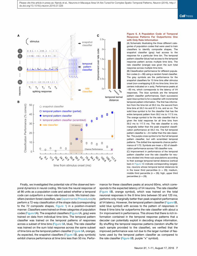
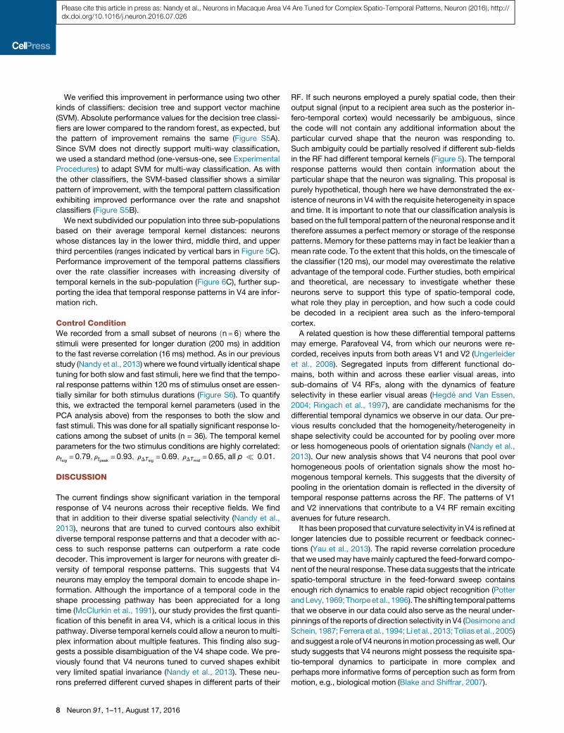
CFigure 6. A Population Code of Temporal
Response Patterns Far Outperforms One
with Only Rate Information
(A) Schematic illustrating the three different cate-
gories of population codes that were used to train
classifiers to identify composite shapes. The
snapshot classifier (gray) had access to the
response for a particular time bin. The temporal
pattern classifier (blue) had access to the temporal
response pattern across multiple time bins. The
rate classifier (orange) was given the sum total
response across multiple time bins.
(B) Classification performance for different popula-
tion codes (n = 86) using a random forest classifier.
The gray symbols are the performance for the
snapshot classifiers for 15 time bins after stimulus
onset (non-overlapping 8.33 ms time bins; time bin
centers indicated on x axis). Performance peaks at
�60 ms, which corresponds to the latency of V4
responses. The blue symbols are the temporal
pattern classifier performances. Each successive
open blue symbol is for a classifier with incremental
temporal pattern information. The first has informa-
tion from the time bin at 59.2 ms, the second from
time bins at 59.2 ms and 67.5 ms, and so on. The
solid blue symbol is for the classifier that has the
entire temporal pattern from 59.2 ms to 117.5 ms.
The orange symbol is for the rate classifier that is
given the total response for all time bins from
59.2 ms to 117.5 ms. The rate classifier is only
marginally better than the peak snapshot classifi-
cation performance at 59.2 ms. The full temporal
pattern classifier is �33 better than the rate classi-
fier. The purple cross symbol is for the full temporal
pattern classifier, but with scrambled temporal
patterns. The dotted line represents chance perfor-
mance of 1/72. Symbols are mean ± SD of classifi-
cation performance across 100 classifier runs.
(C) Improvement in performance of the temporal
pattern classifier over the rate classifier for neu-
rons divided into three sub-populations according
to their average temporal kernel distance (vertical
bars in Figure 5C indicate corresponding ranges):
low, neurons whose temporal kernel distances lie
in the lower third percentiles (n = 29); medium,
middle third percentile (n = 28); high, upper third
percentiles (n = 29).
Please cite this article in press as: Nandy et al., Neurons in Macaque Area V4 Are Tuned for Complex Spatio-Temporal Patterns, Neuron (2016), http://dx.doi.org/10.1016/j.neuron.2016.07.026
Finally, we investigated the potential role of the observed tem-
poral dynamics in neural coding. We took the neural response of
all 86 units as a population code and asked whether a temporal
code can outperform a mean-rate-based code. We trained clas-
sifiers (random forest classifiers, see Experimental Procedures) to
perform a 72-way classification of the shape data (corresponding
to the 72 composite shapes, Figure 1) in a position-invariant
manner. Classifierswere trained on three categories of population
codes (Figure 6A). The snapshot classifiers (Figure 6A, gray) were
trained on data from individual time bins. The temporal pattern
classifier was trained on the temporal patterns of responses
across a subset of time bins (Figure 6A, blue). The rate classifier
was trained on the sum total response across the same subset
of time bins as the temporal pattern classifier (Figure 6A, orange).
As expected, the snapshot classifiers (Figure 6B, gray symbols)
exhibit chance performance at time bins less than 50 ms. Perfor-
mance for these classifiers peaks at around 60ms, which corre-
sponds to the expected latency of V4 neurons. The rate classifier
(Figure 6B, orange symbol), which was trained on the total
neuronal responses in the 8 time bins between 50 and 120 ms,
performs only marginally better than peak snapshot performance
at V4 latency. However, the temporal pattern classifier (Figure 6B,
solid blue symbol) with access to the pattern of responses in
these 8 time bins far outperforms the rate classifier with about a
33 improvement in performance. This shows that there is rich in-
formation contained in the temporal response patterns that a
decoder can potentially exploit in decoding shape information.
By shuffling the temporal response patterns (random shuffle for
each sample provided to the classifier), we verified that the
improved performance was not due to the larger number of fea-
tures used by the temporal pattern classifier as compared to
the rate classifier (Figure 6B, purple ‘‘x’’ symbol).
Neuron 91, 1–11, August 17, 2016 7
Please cite this article in press as: Nandy et al., Neurons in Macaque Area V4 Are Tuned for Complex Spatio-Temporal Patterns, Neuron (2016), http://dx.doi.org/10.1016/j.neuron.2016.07.026
We verified this improvement in performance using two other
kinds of classifiers: decision tree and support vector machine
(SVM). Absolute performance values for the decision tree classi-
fiers are lower compared to the random forest, as expected, but
the pattern of improvement remains the same (Figure S5A).
Since SVM does not directly support multi-way classification,
we used a standard method (one-versus-one, see Experimental
Procedures) to adapt SVM for multi-way classification. As with
the other classifiers, the SVM-based classifier shows a similar
pattern of improvement, with the temporal pattern classification
exhibiting improved performance over the rate and snapshot
classifiers (Figure S5B).
We next subdivided our population into three sub-populations
based on their average temporal kernel distances: neurons
whose distances lay in the lower third, middle third, and upper
third percentiles (ranges indicated by vertical bars in Figure 5C).
Performance improvement of the temporal patterns classifiers
over the rate classifier increases with increasing diversity of
temporal kernels in the sub-population (Figure 6C), further sup-
porting the idea that temporal response patterns in V4 are infor-
mation rich.
Control ConditionWe recorded from a small subset of neurons ðn= 6Þ where the
stimuli were presented for longer duration (200 ms) in addition
to the fast reverse correlation (16 ms) method. As in our previous
study (Nandy et al., 2013) where we found virtually identical shape
tuning for both slow and fast stimuli, here we find that the tempo-
ral response patterns within 120 ms of stimulus onset are essen-
tially similar for both stimulus durations (Figure S6). To quantify
this, we extracted the temporal kernel parameters (used in the
PCA analysis above) from the responses to both the slow and
fast stimuli. This was done for all spatially significant response lo-
cations among the subset of units (n = 36). The temporal kernel
parameters for the two stimulus conditions are highly correlated:
rtsig = 0:79; rtpeak = 0:93; rDTsig= 0:69; rDTmid
= 0:65, all p � 0:01.
DISCUSSION
The current findings show significant variation in the temporal
response of V4 neurons across their receptive fields. We find
that in addition to their diverse spatial selectivity (Nandy et al.,
2013), neurons that are tuned to curved contours also exhibit
diverse temporal response patterns and that a decoder with ac-
cess to such response patterns can outperform a rate code
decoder. This improvement is larger for neurons with greater di-
versity of temporal response patterns. This suggests that V4
neurons may employ the temporal domain to encode shape in-
formation. Although the importance of a temporal code in the
shape processing pathway has been appreciated for a long
time (McClurkin et al., 1991), our study provides the first quanti-
fication of this benefit in area V4, which is a critical locus in this
pathway. Diverse temporal kernels could allow a neuron tomulti-
plex information about multiple features. This finding also sug-
gests a possible disambiguation of the V4 shape code. We pre-
viously found that V4 neurons tuned to curved shapes exhibit
very limited spatial invariance (Nandy et al., 2013). These neu-
rons preferred different curved shapes in different parts of their
8 Neuron 91, 1–11, August 17, 2016
RF. If such neurons employed a purely spatial code, then their
output signal (input to a recipient area such as the posterior in-
fero-temporal cortex) would necessarily be ambiguous, since
the code will not contain any additional information about the
particular curved shape that the neuron was responding to.
Such ambiguity could be partially resolved if different sub-fields
in the RF had different temporal kernels (Figure 5). The temporal
response patterns would then contain information about the
particular shape that the neuron was signaling. This proposal is
purely hypothetical, though here we have demonstrated the ex-
istence of neurons in V4with the requisite heterogeneity in space
and time. It is important to note that our classification analysis is
based on the full temporal pattern of the neuronal response and it
therefore assumes a perfect memory or storage of the response
patterns. Memory for these patterns may in fact be leakier than a
mean rate code. To the extent that this holds, on the timescale of
the classifier (120 ms), our model may overestimate the relative
advantage of the temporal code. Further studies, both empirical
and theoretical, are necessary to investigate whether these
neurons serve to support this type of spatio-temporal code,
what role they play in perception, and how such a code could
be decoded in a recipient area such as the infero-temporal
cortex.
A related question is how these differential temporal patterns
may emerge. Parafoveal V4, from which our neurons were re-
corded, receives inputs from both areas V1 and V2 (Ungerleider
et al., 2008). Segregated inputs from different functional do-
mains, both within and across these earlier visual areas, into
sub-domains of V4 RFs, along with the dynamics of feature
selectivity in these earlier visual areas (Hegde and Van Essen,
2004; Ringach et al., 1997), are candidate mechanisms for the
differential temporal dynamics we observe in our data. Our pre-
vious results concluded that the homogeneity/heterogeneity in
shape selectivity could be accounted for by pooling over more
or less homogeneous pools of orientation signals (Nandy et al.,
2013). Our new analysis shows that V4 neurons that pool over
homogeneous pools of orientation signals show the most ho-
mogenous temporal kernels. This suggests that the diversity of
pooling in the orientation domain is reflected in the diversity of
temporal response patterns across the RF. The patterns of V1
and V2 innervations that contribute to a V4 RF remain exciting
avenues for future research.
It has been proposed that curvature selectivity in V4 is refined at
longer latencies due to possible recurrent or feedback connec-
tions (Yau et al., 2013). The rapid reverse correlation procedure
that we usedmay havemainly captured the feed-forward compo-
nent of the neural response. These data suggests that the intricate
spatio-temporal structure in the feed-forward sweep contains
enough rich dynamics to enable rapid object recognition (Potter
andLevy,1969;Thorpeetal., 1996).Theshifting temporalpatterns
that we observe in our data could also serve as the neural under-
pinnings of the reports of direction selectivity in V4 (Desimone and
Schein, 1987; Ferrera et al., 1994; Li et al., 2013; Tolias et al., 2005)
and suggest a role of V4neurons inmotionprocessing aswell. Our
study suggests that V4 neurons might possess the requisite spa-
tio-temporal dynamics to participate in more complex and
perhaps more informative forms of perception such as form from
motion, e.g., biological motion (Blake and Shiffrar, 2007).
Please cite this article in press as: Nandy et al., Neurons in Macaque Area V4 Are Tuned for Complex Spatio-Temporal Patterns, Neuron (2016), http://dx.doi.org/10.1016/j.neuron.2016.07.026
EXPERIMENTAL PROCEDURES
Electrophysiology
Neurons were recorded in area V4 in two rhesus macaques. Surgical and elec-
trophysiological procedures have been described previously (Nandy et al.,
2013; Reynolds et al., 1999). In brief, a recording chamber was placed over
the prelunate gyrus, on the basis of preoperative MRI imaging. All procedures
were approved by the Institutional Animal Care and Use Committee and con-
formed to NIH guidelines. Neuronal signals were recorded extracellularly,
filtered, and stored using the Multichannel Acquisition Processor system
(Plexon). Single units were isolated in the Plexon Offline Sorter based on wave-
form shape and were included only if they formed an identifiable cluster, sepa-
rate from noise and other units, when projected into the principal components
of waveforms recorded on that electrode.
Task, Stimuli, and Inclusion Criteria
Experimental procedures have been described in detail previously (Nandy
et al., 2013). In brief, stimuli were presented on a computer monitor placed
57 cm from the eye. Eye position was continuously monitored with an infrared
eye tracking system. Trials were aborted if eye position deviated more than 1�
from fixation. Experimental control was handled by NIMH Cortex software
(http://www.cortex.salk.edu/). At the beginning of each recording session,
preliminary neuronal RFs were mapped using subspace reverse correlation
in which Gabor (eight orientations, 80% luminance contrast, spatial frequency
1.2 cpd, Gaussian half-width 2�) or ring stimuli (80% luminance contrast) ap-
peared at 60 Hz.
For the main task, the monkey began each trial by fixating a central point for
200 ms and then maintained fixation through the trial. Each trial lasted 3 s dur-
ing which neuronal responses to a fast-reverse correlation sequence (16 ms
stimulus duration, exponential distributed delay between stimuli with mean
delay of 16 ms, i.e., 0 ms delay p = 1/2, 16 ms delay p = 1/4, 32 ms delay
p = 1/8 and so on) were recorded. The stimuli were comprised of oriented
bars (8 orientations) or bar composites (16 orientations3 5 conjunction angles,
total of 72 unique stimuli; Figure 1). The five conjunction levels created five cat-
egories of shapes: zero curvature/straight, low curvature, medium curvature,
high curvature, and ‘‘C.’’ A pseudo-random sequence from the combined
stimulus sets was presented in each trial. The composite stimuli were pre-
sented on a uniform 535 location grid (‘‘coarse grid’’) centered on the esti-
mated spatial RF based on the preliminary mapping. The grid locations were
separated by one-fourth of the RF eccentricity (e.g., for a RF centered at 6�,the grid-spacing was 1.5� and the grid covered a visual extent of 3�–9�). Theoriented bar stimuli were presented on a finer 15315 location grid (‘‘fine
grid’’) that spanned the larger 535 grid in equal-spaced increments. Stimuli
were scaled by RF eccentricity such that each single bar element spanned
approximately the diagonal length of the fine grid. The receptive fields of all
neurons reported in the study were in the parafoveal region between 2� and
12� in the inferior right visual field.
Only well-isolated units were considered as potential candidates for the
analysis. Among these, only those neurons that were significantly spatially
responsive and shape selective were selected for further analysis (n = 86).
The details of inclusion criteria have been described previously (Nandy et al.,
2013). In brief, we first determined a spatial Z score for each location on the
535 grid based on the average response across all composite stimuli at the
spatial location. A grid location was marked as spatially significant if it ex-
ceeded the significance level of 0.05 (corrected for 25 multiple comparisons).
We next determined if the neuron was significantly shape selective at that
spatial location by calculating a shape Z score for each composite shape.
The spatial location was considered as shape selective if the maximum among
the shape Z scores exceeded the 0.05 significance level (corrected for 723M
multiple comparisons, where M = the number of spatially significant grid loca-
tions). A neuron was considered significantly shape selective if it had at least
one spatially significant grid location that was also significantly shape
selective.
Data Analysis
Spatio-temporal receptive fields (STRFs) were computed as follows: a tempo-
ral window between 30 and 120 ms after stimulus onset was used to identify a
temporal interval of significant visual response, Tsig. The temporal windowwas
divided into non-overlapping 8.33 ms bins for determining the peri-stimulus
time histogram (PSTH). Tsig was taken as those PSTH bins where the mean
firing rate averaged across all stimulus conditions exceeded the baseline
rate by 4 standard deviations. The baseline rate was determined from a tem-
poral window between 0 and 20 ms after stimulus onset. For each significant
time bin, we determined the neuronal response, rðx; y; s; ti ; ti ˛TsigÞ to a partic-
ular stimulus, s, at grid location ðx; yÞ, as the average firing rate across stimulus
repeats. This was done separately for the composite stimuli and the oriented
bars to yield STRFs at both the coarse (Figure 4) and fine (Figure 2, upper
panels) spatial scales.
Estimation of Temporal Trajectories of the Fine-Scale STRFs
The fine-scale STRF was first averaged across all eight orientations for each
spatial location, brðx; y; ti ; ti ˛TsigÞ. This orientation averaged STRF was
spatially interpolated using 2D nearest neighbor interpolation (20 interpolation
points, Figure 2, lower panels). We calculated response contours at 90%,
80%, 70%, 60%, and 50% of local peak at each significant time bin (Figure 2,
lower panels), and further, the centroid of each contour. The trajectory of the
centroids across the spatial extent of the RF (Figures 3A and S1C) was then
used to compute the spatial excursion of the temporal response (Figure 3B).
The spatial excursion was quantified as follows: for each trajectory, we calcu-
lated the maximum Euclidean distance ðDmaxÞ between any pair of points on
the trajectory. We also estimated the spatial extent of the RF as the length
of themajor axis ðDRFÞ of the least-squares best-fit ellipse to the 50% response
contour of the temporally averagedRF (i.e., average across all STRF significant
time bins). We used the normalized maximum Euclidean distance as a mea-
sure of the spatial excursion of the temporal response:
Dnorm =Dmax
DRF
:
To obtain error bounds on this estimate, we performed a jackknife analysis
on the data (Nj = 20 jackknifes, each using 95% of trials). For each jackknife,
we calculated contour centroids at each response level (90%, 80%, .,
50%). We thus obtained 20 centroid trajectories for each response level (Fig-
ures 3A and S1C; colored lines). We then estimated Dnorm by calculating Dmax
(using the same time bins that contributed to Dmax in the full dataset) and DRF
for each jackknife.
To estimate whether these spatial excursions were statistically significant,
we calculated a distribution of null trajectories as follows: we reasoned that
if spatial selectivity within the RF did not have temporal structure, then the sta-
tistics of trajectories obtained by temporal shuffling will not be significantly
different from the original (unshuffled) trajectories; if, on the other hand, spatial
selectivity had specific temporal signatures, then the shuffled trajectories will
be markedly different. We first generated temporally shuffled versions of the
orientation averaged STRF, br shuffledðx; y; ti ; ti ˛Tsig�permuteÞ, by random permu-
tations of the response values across time for each spatial location ðx; yÞ. Toavoid non-stationarity in the mean temporal responses (averaged across
spatial positions) due to shuffling, we first normalized the data per time bin
prior to shuffling. For each shuffled STRF we obtained the temporal trajectory
of the contour centroids (gray trajectories in Figures 3A and S1C) and the
normalized maximum distance ðDnorm�shuffledÞ as with the original unshuffled
data (using the same time bins that contributed to Dmax in the unshuffled
data). This was repeated 1,000 times to obtain a distribution of null temporal
excursions.
Temporal Stability of Shape Tuning
To examine the stability of the coarse-scale STRFs over time, we computed
the peak shape selectivity (centroid of contour at 90% of peak response)
across significant temporal bins at the maximally responsive spatial location
on the 535 grid (Figures 4A and 4B). We computed a dispersion metric for
shape selectivity as the ratio of the area of the convex hull of the peak response
locations across time in shape space (dotted polygons in Figure 4B) over the
area of the entire shape space (Figure 4C). Stability of shape tuning would
imply a low dispersion metric. To estimate whether the dispersion was statis-
tically significantly different from a null distribution, we performed a bootstrap
analysis on temporally shuffled data that was essentially similar to the
Dnorm�shuffled procedure described above, but performed on the coarse-scale
Neuron 91, 1–11, August 17, 2016 9
Please cite this article in press as: Nandy et al., Neurons in Macaque Area V4 Are Tuned for Complex Spatio-Temporal Patterns, Neuron (2016), http://dx.doi.org/10.1016/j.neuron.2016.07.026
data. We thus obtained a null distribution of the dispersion metric against
which to compare the metric from the empirical data in order to assess statis-
tical significance.
Pairwise Pattern Correlation for Composite Stimuli
As described previously (Nandy et al., 2013), for each neuron we first deter-
mined the spatial locations with significant response on the 535 coarse grid.
For each pair of spatially significant coarse grid locations, we then estimated
the empirical distribution of correlation coefficients between the response pat-
terns to the composite stimuli at the two locations using a bootstrap procedure
(Efron and Tibshirani, 1993). The response patterns were calculated from the
average response to each composite shape across all significant time bins,
Tsig. The pairwise pattern correlation ðrÞ was taken as the expected value of
a Gaussian fit to this empirical distribution (see Figure S4 in Nandy et al.,
2013). Pairwise pattern correlations for example neurons are shown in Fig-
ure S4 (middle column).
Pairwise Temporal Kernel Distance for Composite Stimuli
For each significant spatial location ðx; yÞ on the 535 grid, we calculated the
temporal kernelKx;yðtÞ as the average time course to the set of composite stim-
uli, which elicited responses that were above 70% of local peak in the tempo-
rally averaged responses brðx; y; sÞ (averaged across all significant time bins).
For each temporal kernel, we calculated (a) the time point, tsig, at which the
response first reached significance (4 standard deviations above baseline;
baseline calculated from a time window between 0 and 20 ms from stimulus
onset), (b) the duration, DTsig, over which the response remained significant,
(c) the time point, tpeak, at which the response reached its peak, and (d) the
duration, DTmid, over which the response was above the half-way mark be-
tween peak response and baseline (Figure 5B). Each temporal kernel can be
represented as a point in a 4D space defined by tsig, DTsig, tpeak, and DTmid.
We then performed a principal components analysis (PCA) on this 4D space
(Figures S3D and S3E). The first two principal components accounted for
88% of the variance in the data (Figure S3E). We then projected each point
in the 4D space to the lower dimensional 2D plane defined by the two principal
components (Figure S3D). The Euclidean distance, D, between pairs of points
in this 2D plane serves as a measure of similarity between temporal kernels.
Such pairwise distances for example neurons are shown in Figure S4 (right
column).
Shape Classification
For each neuron in our population, we calculated the empirical distribution of
firing rates in 8.33ms non-overlapping time bins within a temporal window 0 to
120 ms after stimulus onset, using a bootstrap procedure (resampling with
replacement, 1,000 iterations) (Efron and Tibshirani, 1993). This was done
separately for each of the 72 composite stimuli on each of the 25 spatial loca-
tions in the 535 coarse grid. Firing rates were normalized to a neuron’s peak
response. Each of the empirical distributions was very well fit with a Gaussian.
In this fashion, we obtained a statistical description of the firing rate for
each {neuron [n = 86], spatial location [n = 25], stimulus [n = 72], time bin
[n = 16]}-tuple. We chose the resampling approach since stimulus repeats var-
ied across neurons due to varying durations of isolation and also due to the
pseudo-random presentation sequences for the fast reverse-correlation pro-
cedure (28:3±4:2 presentations across all neurons, locations, and stimuli).
We next trained classifiers to perform a 72-way classification of stimulus iden-
tity in a position-invariant manner as follows. For each sample that was input to
the classifier, we first chose a random location on the 535 grid and a random
stimulus identity from the set of 72. For this combination of location and
stimulus, we generated a population response vector, which along with the
stimulus identity (scalar, [1.72]) served as a training or a test sample for the
classifiers. We assessed classification performance for three categories of
population codes. (a) Snapshot classifier: for this classifier, the population
response vector consisted of responses (drawn from the empirical distribu-
tions) from a particular time bin for each neuron (Figure 6A, gray). We had 16
such classifiers for each of the 16 time bins. (b) Temporal pattern classifier:
here the population response vector consisted of the train (or pattern) of re-
sponses across a subset of time bins for each neuron (Figure 6A, blue). (c)
Rate classifier: here the population response vector consisted of the sum of
the responses across a subset of time bins for each neuron (Figure 6A, orange).
For each classification run, 3,000 such population vector samples along with
the corresponding stimulus identities were given to the classifier for training
10 Neuron 91, 1–11, August 17, 2016
and testing with cross-validation. We assessed classification performance us-
ing both an ensemble-based random forest classifier (Breiman, 2001) (Fig-
ure 6B) and a decision tree classifier (Rokach andMaimon, 2008) (Figure S5A).
A random forest is a meta-estimator that fits a number of decision tree classi-
fiers on various sub-samples of the dataset and uses averaging to improve the
predictive accuracy and control over-fitting. The sub-sample size is always the
same as the original input sample size, but the samples are drawn with
replacement. Classification performance for the random forest classifiers
was reported as 1� OutOfBagError (Breiman, 1996). We used random for-
est classifiers with 50 decision trees, as this was the number of trees for which
the OutOfBagError was saturated. Classification performance for the deci-
sion tree classifiers was the 10-fold cross-validated performance (90% of
samples used for training, 10% for test; 10 such runs leaving out independent
sets for test).
We also assessed classification performance using a more traditional sup-
port vector machine (SVM) approach with a linear kernel (Figure S5B).
Since SVM does not directly support multi-way classification, we used a
one-versus-one (OVO), also known as an all-versus-all, approach (Hastie
and Tibshirani, 1998) to build a bank of binary classifiers whose predictions
are combined using hamming decoding to generate the multi-way classifica-
tion (Allwein et al., 2000). For each stimulus pair, we trained a binary classifier
to perform a positive-class versus negative-class categorization. With 72
unique stimuli, we thus had a total of
�722
�= 2; 556 binary classifiers whose
predictions were combined as described in Allwein et al. (2000) to achieve
the multi-class classification. The number of training samples was reduced
from 3,000 to 500 in order to prevent boosting due to the large number of
binary classifiers in the multi-way SVM. Classification performance was as-
sessed with 10-fold cross validation. Machine learning software for all three
types of multi-way classification analyses was implemented in MATLAB
(r2014b) using the Statistics Toolbox.
SUPPLEMENTAL INFORMATION
Supplemental Information includes six figures and can be found with this
article online at http://dx.doi.org/10.1016/j.neuron.2016.07.026.
AUTHOR CONTRIBUTIONS
A.S.N. and J.F.M. designed the experiments, collected data, and developed
the statistical methods. A.S.N. analyzed the data. A.S.N. and M.P.J. devel-
oped the classification model. All authors contributed to writing the
manuscript.
ACKNOWLEDGMENTS
This research was supported by NIH R01 EY021827 to J.H.R. and A.S.N., the
Gatsby Charitable Foundation to J.H.R., the Swartz Foundation to J.F.M., fel-
lowships from the NIH T32 EY020503 training grant and the Salk Institute
Pioneer Fund to A.S.N., NIH 5K99 EY025026-02 to M.P.J., and a NEI core
grant for vision research P30 EY019005 to the Salk Institute. We would like
to thank Terrence Sejnowski and Saket Navlakha for helpful discussions and
Catherine Williams for excellent animal care.
Received: August 10, 2015
Revised: April 9, 2016
Accepted: July 11, 2016
Published: August 4, 2016
REFERENCES
Allwein, E.L., Schapire, R., and Singer, Y. (2000). Reducing Multiclass to
Binary: A Unifying Approach for Margin Classifiers. J. Mach. Learn. Res. 1,
113–141.
Anzai, A., Peng, X., and Van Essen, D.C. (2007). Neurons in monkey visual area
V2 encode combinations of orientations. Nat. Neurosci. 10, 1313–1321.
Please cite this article in press as: Nandy et al., Neurons in Macaque Area V4 Are Tuned for Complex Spatio-Temporal Patterns, Neuron (2016), http://dx.doi.org/10.1016/j.neuron.2016.07.026
Blake, R., and Shiffrar, M. (2007). Perception of human motion. Annu. Rev.
Psychol. 58, 47–73.
Breiman, L. (1996). Bagging Predictors. Mach. Learn. 24, 123–140.
Breiman, L. (2001). Random Forests. Mach. Learn. 45, 5–32.
Desimone, R., and Schein, S.J. (1987). Visual properties of neurons in area V4
of the macaque: sensitivity to stimulus form. J. Neurophysiol. 57, 835–868.
DiCarlo, J.J., Zoccolan, D., and Rust, N.C. (2012). How does the brain solve
visual object recognition? Neuron 73, 415–434.
Efron, B., and Tibshirani, R.J. (1993). An introduction to the bootstrap
(Chapman & Hall/CRC).
Ferrera, V.P., Rudolph, K.K., and Maunsell, J.H. (1994). Responses of neurons
in the parietal and temporal visual pathways during a motion task. J. Neurosci.
14, 6171–6186.
Field, G.D., and Chichilnisky, E.J. (2007). Information processing in the primate
retina: circuitry and coding. Annu. Rev. Neurosci. 30, 1–30.
Field, G.D., Gauthier, J.L., Sher, A., Greschner, M., Machado, T.A., Jepson,
L.H., Shlens, J., Gunning, D.E., Mathieson, K., Dabrowski, W., et al. (2010).
Functional connectivity in the retina at the resolution of photoreceptors.
Nature 467, 673–677.
Hastie, T., and Tibshirani, R. (1998). Classification by pairwise coupling. Ann.
Stat. 26, 451–471.
Hegde, J., and Van Essen, D.C. (2004). Temporal dynamics of shape analysis
in macaque visual area V2. J. Neurophysiol. 92, 3030–3042.
Jin, J.,Wang, Y., Swadlow, H.A., and Alonso, J.M. (2011). Population receptive
fields of ON and OFF thalamic inputs to an orientation column in visual cortex.
Nat. Neurosci. 14, 232–238.
Li, P., Zhu, S., Chen, M., Han, C., Xu, H., Hu, J., Fang, Y., and Lu, H.D. (2013). A
motion direction preference map in monkey V4. Neuron 78, 376–388.
McClurkin, J.W., Optican, L.M., Richmond, B.J., and Gawne, T.J. (1991).
Concurrent processing and complexity of temporally encoded neuronal mes-
sages in visual perception. Science 253, 675–677.
Nandy, A.S., Sharpee, T.O., Reynolds, J.H., and Mitchell, J.F. (2013). The fine
structure of shape tuning in area V4. Neuron 78, 1102–1115.
Pasupathy, A., and Connor, C.E. (1999). Responses to contour features in ma-
caque area V4. J. Neurophysiol. 82, 2490–2502.
Pasupathy, A., and Connor, C.E. (2001). Shape representation in area V4: po-
sition-specific tuning for boundary conformation. J. Neurophysiol. 86, 2505–
2519.
Pasupathy, A., and Connor, C.E. (2002). Population coding of shape in area V4.
Nat. Neurosci. 5, 1332–1338.
Potter, M.C., and Levy, E.I. (1969). Recognition memory for a rapid sequence
of pictures. J. Exp. Psychol. 81, 10–15.
Reynolds, J.H., Chelazzi, L., and Desimone, R. (1999). Competitive mecha-
nisms subserve attention in macaque areas V2 and V4. J. Neurosci. 19,
1736–1753.
Ringach, D.L., Hawken, M.J., and Shapley, R. (1997). Dynamics of orientation
tuning in macaque primary visual cortex. Nature 387, 281–284.
Rokach, L., and Maimon, O. (2008). Data Mining with Decision Trees: Theory
and Applications (World Scientific Publishing).
Rust, N.C., and Dicarlo, J.J. (2010). Selectivity and tolerance (‘‘invariance’’)
both increase as visual information propagates from cortical area V4 to IT.
J. Neurosci. 30, 12978–12995.
Schwartz, G.W., Okawa, H., Dunn, F.A., Morgan, J.L., Kerschensteiner, D.,
Wong, R.O., and Rieke, F. (2012). The spatial structure of a nonlinear receptive
field. Nat. Neurosci. 15, 1572–1580.
Tao, X., Zhang, B., Smith, E.L., 3rd, Nishimoto, S., Ohzawa, I., and Chino, Y.M.
(2012). Local sensitivity to stimulus orientation and spatial frequency within
the receptive fields of neurons in visual area 2 of macaque monkeys.
J. Neurophysiol. 107, 1094–1110.
Thorpe, S., Fize, D., and Marlot, C. (1996). Speed of processing in the human
visual system. Nature 381, 520–522.
Tolias, A.S., Keliris, G.A., Smirnakis, S.M., and Logothetis, N.K. (2005).
Neurons in macaque area V4 acquire directional tuning after adaptation tomo-
tion stimuli. Nat. Neurosci. 8, 591–593.
Ungerleider, L.G., Galkin, T.W., Desimone, R., and Gattass, R. (2008). Cortical
connections of area V4 in the macaque. Cereb. Cortex 18, 477–499.
Yau, J.M., Pasupathy, A., Brincat, S.L., and Connor, C.E. (2013). Curvature
processing dynamics in macaque area V4. Cereb. Cortex 23, 198–209.
Neuron 91, 1–11, August 17, 2016 11
Neuron, Volume 91
Supplemental Information
Neurons in Macaque Area V4 Are Tuned
for Complex Spatio-Temporal Patterns
Anirvan S. Nandy, Jude F. Mitchell, Monika P. Jadi, and John H. Reynolds
!
1
!!
Supplementary Information: Neurons in macaque Area V4 are tuned for complex spatio-temporal patterns
Anirvan S. Nandy1, Jude F. Mitchell1,3, Monika P. Jadi2 & John H. Reynolds1
1Systems & 2Computational Neurobiology Laboratories
The Salk Institute for Biological Studies, La Jolla, CA 92037
3Current address: Dept. of Brain & Cognitive Sciences, University of Rochester,
Rochester, NY 14627
Corresponding author: A.S.N. ([email protected])
Supplementary Figure-1 NANDY
I
II
I
I
II
II
59.17 ms 67.50 ms 75.83 ms 84.17 ms 92.50 ms 100.83 ms 109.17 ms 117.50 ms
50.83 ms 59.17 ms 67.50 ms 75.83 ms 84.17 ms 92.50 ms 100.83 ms 109.17 ms
1 dv
a0.
5 dv
a1
dva
0.5
dva
A
C
D E
B
00 0.1 0.2 0.3 0.4 0.5 0.6
0.01
0.02
0.03
0.04
Dnorm
Dey
e-po
sitio
n (d
va)
ρ=0.05 (p=0.65), n=86
90% 80% 70% 60% 50%
full datafirst 50%last 50%
0.10 0.2 0.3 0.4 0.5 0.60
0.1
0.2
0.3
0.4
0.5
0.6
Dno
rm (l
ast 5
0%)
Dnorm (first 50%)
ρ = 0.6 (p<<0.01), n=86
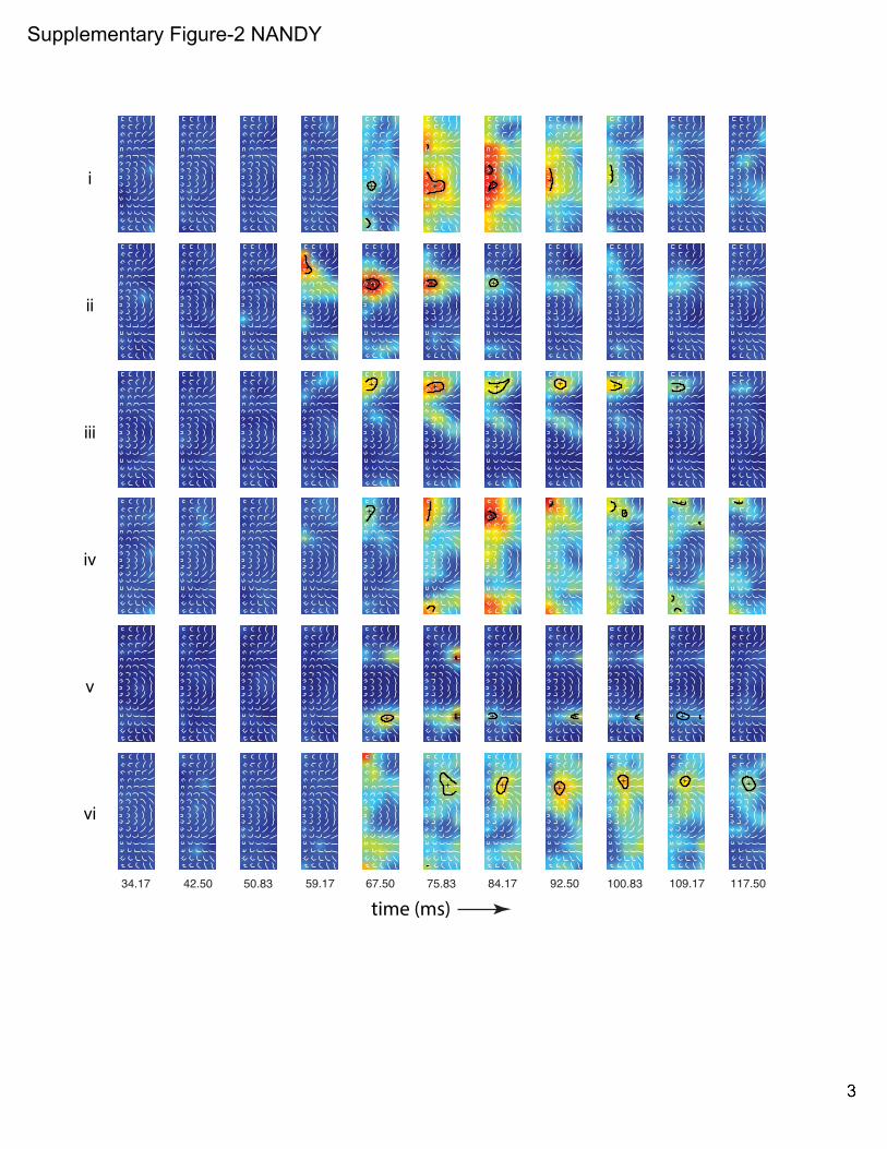
Supplementary Figure-2 NANDY
i
ii
iii
iv
v
vi
50.8342.5034.17 59.17 67.50 75.83 84.17 92.50 100.83 109.17 117.50
time (ms)
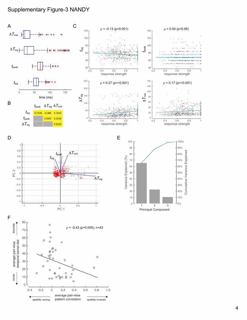
Supplementary Figure-3 NANDY
A
B
C
D
F
E
0 50 100 150
tsig
tsig
t sig
tpeak
tpeak
tpeak
t peakTsig
Tsig
Tsig
T sig
Tmid
Tmid
T mid
time (ms)
Principal Component
Var
ianc
e E
xpla
ined
(%)
Cum
ulat
ive
Var
ianc
e E
xpla
ined
0
10
20
30
40
50
60
70
80
90
100
0%
10%
20%
30%
40%
50%
60%
70%
80%
90%
100%
1 2 3PC 1
-1 -0.5 0 0.5 1
PC
2
-1
-0.8
-0.6
-0.4
-0.2
0
0.2
0.4
0.6
0.8
1
Tsig
tsig
tpeak Tmid
response strength response strength
response strengthresponse strength
0.2 0.4 0.6 0.8 1 0.2 0.4 0.6 0.8 1
0.2 0.4 0.6 0.8 10.2 0.4 0.6 0.8 1
20
40
60
80
100
120
40
60
80
100
120
140
0
50
100
150
200
250
0
20
40
60
80
100
120
140
ρ = -0.13 (p=0.001)
ρ = 0.27 (p<<0.001) ρ = 0.17 (p<<0.001)
ρ = 0.00 (p=0.95)
0.7339 -0.386
0.0937
0.1623
0.3539
0.3223
-0.4 -0.2 0 0.2 0.4 0.6 0.8 1.00
10
20
30
40
50
60
70
80
aver
age
pair-
wis
e te
mpo
ral k
erne
l dis
tsi
mila
rdi
ssim
ilar
average pair-wise pattern correlation spatially invariantspatially varying
ρ = -0.43 (p=0.005), n=43
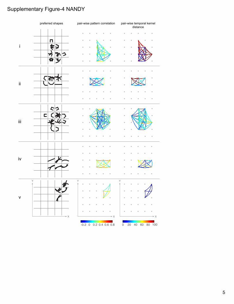
Supplementary Figure-4 NANDY
-0.2 0 0.2 0.4 0.6 0.8 0 20 40 60 80 100
pair-wise pattern correlationpreferred shapes pair-wise temporal kernel distance
X
Y
X
Y
X
Y
i
ii
iii
iv
v
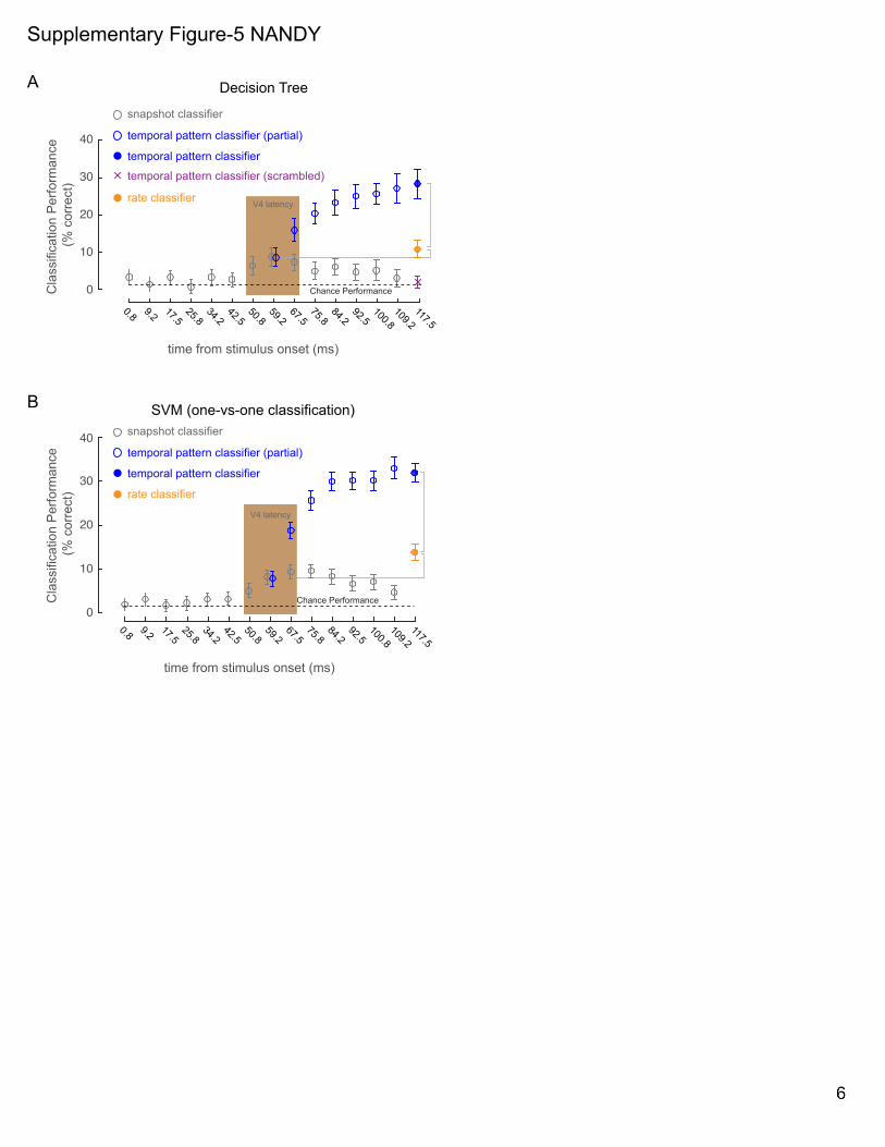
Supplementary Figure-5 NANDYC
lass
ifica
tion
Per
form
ance
(% c
orre
ct)
Cla
ssifi
catio
n P
erfo
rman
ce (%
cor
rect
)
time from stimulus onset (ms)
59.250.8
42.534.2
25.817.5
9.20.8 67.575.8
84.292.5
100.8109.2
117.5
Chance Performance0
10
20
30
40
0
10
20
30
40
V4 latency
V4 latency
snapshot classifier
temporal pattern classifier (partial)
temporal pattern classifier
rate classifier
temporal pattern classifier (scrambled)
snapshot classifier
temporal pattern classifier (partial)
temporal pattern classifier
rate classifier
A
B
Decision Tree
time from stimulus onset (ms)
59.250.8
42.534.2
25.817.5
9.20.8 67.575.8
84.292.5
100.8109.2
117.5
SVM (one-vs-one classification)
Chance Performance
Supplementary Figure-6 NANDY
fast (16ms flash)
j_103_u1
slow(200ms flash)
fast
j_101_u1
slow
50.8342.5034.17 59.17 67.50 75.83 84.17 92.50 100.83 109.17 117.50
time (ms)
A
B
0 50 100
0 50 100
0 50 100
0 50 100
t (ms)
j_103_u1 j_101_u1
fast
slow
fast
slow
!
27
!!
SUPPLEMENTARY FIGURE LEGENDS
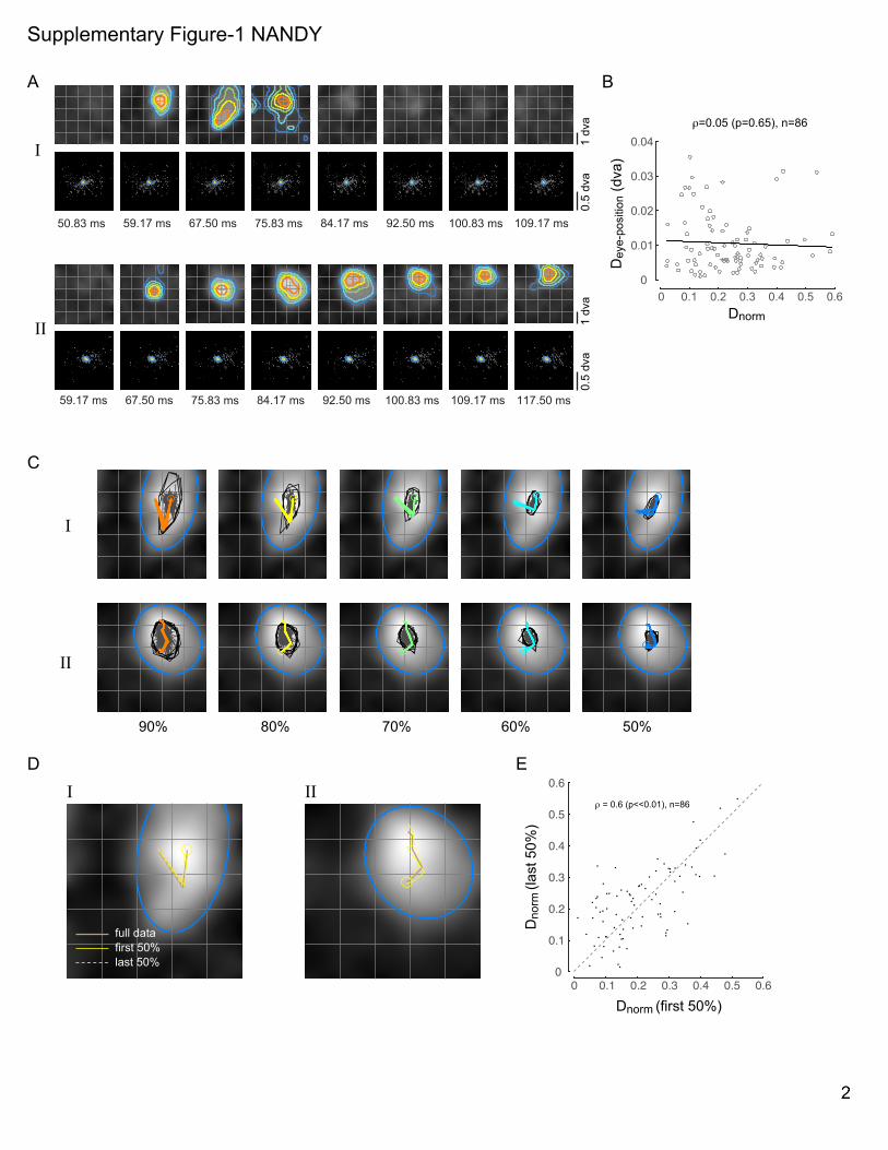
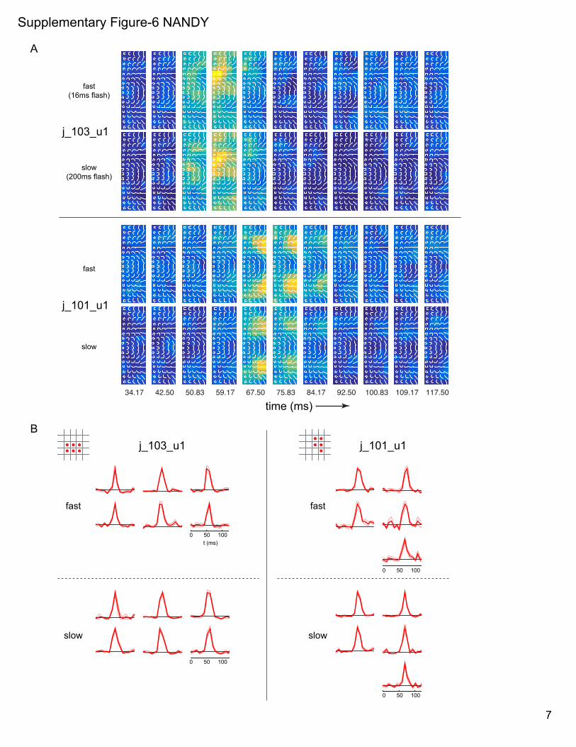
Supp Fig 1. Independence of fine-scale STRFs from fixational eye-movements and the stability of spatial trajectories. Related to Figs 2-3. (A) For 2 example neurons (neurons I & II in Fig 2): Upper panels, temporal evolution of fine-scale STRFs (same format as in Fig 2, lower panels). Lower panels, corresponding distribution of eye-positions. dva: degree of visual angle. (B) Scatter-plot of the maximum spatial excursion of STRF trajectories (!norm, Fig 3) versus the maximum dispersion of eye-position (!eye!position; calculated from the same time-bins used to calculate !norm) show no correlation between the two quantities. (C) Stability of spatial trajectories across response levels: spatial trajectories are shown for the same example neurons in A at 5 response levels (90, 80, 70, 60 and 50% of local peak). Same format as in Fig 3A. (D) Stability of spatial trajectories over measurement duration: spatial trajectories are shown for the same two example neurons in A and B for the full data set, the first 50% of trials and the last 50% of trials. (E) The normalized spatial excursions of the trajectories, !norm, for the first 50% of trials versus the last 50% of trials are plotted for the population of neurons. The two measurements are highly correlated (! = 0.6, ! ≪ 0.01). Supp Fig 2. Coarse-scale STRFs. Related to Fig 4. Neuronal response maps to the set of composite shapes (overlaid in white) are shown for six example neurons (rows) at their respective most responsive spatial location on the 5x5 response grid. Response contours at 90% of local peak are superimposed for all significant time bins (see Experimental Procedures). ‘+’ signs depict the centroids of the contour lines. Supp Fig 3. Principal components analysis on the temporal response profiles. Related to Fig 5. (A) The box-plots show the distribution of the four parameters, !sig, !!sig,!!peak and !!mid (Fig 5) that were extracted from the temporal response profiles at each spatially significant location for all neurons in the population. On each box, the central mark is the median; the edges of the box are the 25th and 75th percentiles. (B) Correlation (Spearman’s !) among the four parameters in A. !sig are !peak are strongly positively correlated. !sig and !!sig are negatively correlated. (C) Scatter-plot of the four parameters in A versus the normalized peak response at the corresponding spatial location in the receptive field. The responses were normalized by each neuron’s maximum response across all spatial locations. !sig has weak negative correlation with response strength. !!sig and !!mid respectively show modest and weak positive correlation with response strength. There is no correlation between !peak and response strength. (D) Each dot is a projection of points in the 4D space (defined by the parameters in A) onto the 2D plane defined by the first two principal components. The four vectors (blue) indicate how each of the four parameters contributes to the two principal components. The projections of the vectors onto the two principal component axes are the coefficients of the principal components. (E) The variance explained by the top 3 principal components in the space defined by the 4 parameters in A, and the cumulative variance explained. (F) The average pair-wise temporal kernel distance is plotted against the average pair-wise pattern correlation (same format as in Fig 5C) for the subset of neurons whose !norm values are in the top 50th percentile (n=43). There is a significant negative correlation (Spearman’s ! = −0.43, ! =0.005) between the two quantities. Supp Fig 4. Preferred shapes, pair-wise pattern correlation and pair-wise temporal kernel distance. Related to Fig 5. Preferred shapes at different spatial locations (left column), response pattern correlation between pairs of spatial locations (middle column) and temporal kernel distance between pairs of spatial locations (right column) are shown for 5 example units (rows). Left column: the location-specific shape or set of shapes to which the neuron responded preferentially, at all spatially significant locations. Shapes are spatially superimposed at each grid location. Middle column: The undirected graphs show the pattern correlation (Pearson correlation between the response patterns to the set of composite shapes at a pair of spatial locations, see Experimental Procedures) for all possible location pairs with significant response. Warmer colors indicate that the location pairs have similar shape selectivity, while cooler colors indicate dissimilar shape selectivity. Right column: The undirected graphs show the distance, !, between pairs of temporal kernels (see Experimental Procedures) for all possible location pairs with significant
!
28 !
response. Coolers colors indicate that location pairs have similar temporal response patterns, while warmer colors indicate dissimilar temporal response patterns. The examples are arranged such that the ones near the top are spatially varying in their shape selectivity, while those near the bottom are spatially invariant. The pair-wise pattern correlations for the neurons with spatially varying tuning (e.g. neurons i and ii) are dominated by low-values (cold colors), while their pair-wise temporal kernel distance are dominated by high values (warm colors). The reverse pattern is seen for neurons with spatially invariant tuning (e.g. neurons iv and v). Supp Fig 5. Related to Fig 6. A population code of temporal response patterns far outperforms one with only rate information. (A) 72-way shape classification performance for different categories of population codes using decision tree classifiers. Same format as in Fig 6B. Symbols are mean ± std. dev. classification performance for 10-fold cross-validated classification. (B) Shape classification for the different categories of population codes using support vector machine (SVM) classifiers with a linear kernel. Since SVM does not directly support multi-way classification, a one-versus-one (OVO) approach was used. Symbols are mean ± std. dev. classification performance for 10-fold cross-validated classification. Supp Fig 6. Related to Figs 2-4. Temporal response patterns are independent of stimulus duration. (A) Neuronal response maps for two example neurons (rows), to the set of composite stimuli (overlaid in white) at their maximally responsive spatial location for fast (16ms duration; upper panels) and slow (200ms; lower panels) stimulus presentations. The temporal response patterns are virtually identical. (B) Normalized temporal response profiles (mean ± s.e.m.) for the same example neurons in A, at all spatially significant response locations on the 5x5 response grid (locations marked with red dots).