Functional Clusters of Neurons in Layer 6 of Macaque V1

Systems/Circuits

Functional Clusters of Neurons in Layer 6 of Macaque V1

Michael J. Hawken, Robert M. Shapley, Anita A. Disney, Virginia Garcia-Marin, Andrew Henrie, Christopher A. Henry,Elizabeth N. Johnson, Siddhartha Joshi, X Jenna G. Kelly, X Dario L. Ringach, and X Dajun XingCenter for Neural Science, New York University, New York, New York 10003

Layer 6 appears to perform a very important role in the function of macaque primary visual cortex, V1, but not enough is understoodabout the functional characteristics of neurons in the layer 6 population. It is unclear to what extent the population is homogeneous withrespect to their visual properties or if one can identify distinct subpopulations. Here we performed a cluster analysis based on measure-ments of the responses of single neurons in layer 6 of primary visual cortex in male macaque monkeys (Macaca fascicularis) to achromaticgrating stimuli that varied in orientation, direction of motion, spatial and temporal frequency, and contrast. The visual stimuli werepresented in a stimulus window that was also varied in size. Using the responses to parametric variation in these stimulus variables,we extracted a number of tuning response measures and used them in the cluster analysis. Six main clusters emerged along with somesmaller clusters. Additionally, we asked whether parameter distributions from each of the clusters were statistically different. There wereclear separations of parameters between some of the clusters, particularly for f1/f0 ratio, direction selectivity, and temporal frequencybandwidth, but other dimensions also showed differences between clusters. Our data suggest that in layer 6 there are multiple parallelcircuits that provide information about different aspects of the visual stimulus.

Key words: layer 6; primate; visual cortex

IntroductionThe study was motivated by the growing realization that layer 6has multiple functional roles in the visual function of macaque

primary visual cortex, V1. Layer 6 provides major output fromV1 to extrastriate (Fries et al., 1985) and subcortical targets (Fitz-patrick et al., 1994) that have different functional characteristics.Layer 6 also has multiple distinct intracortical recurrent pathwaysand provides long-range connections within the infragranularlayers of V1. Layer 6 feedback afferents (McGuire et al., 1984;Wiser and Callaway, 1996) provide a considerable fraction of theexcitatory synapses in V1 layer 4C. Furthermore, such layer 6feedback to layer 4C is provided by distinct subpopulations(Wiser and Callaway, 1996) and appears to be of considerableimportance in the generation of the dynamical responses withinlayer 4C� (Chariker et al., 2016, 2018).

The goal of the current study was to examine layer 6 neuronresponses along multiple stimulus dimensions to seek functional

Received June 14, 2019; revised Jan. 26, 2020; accepted Jan. 27, 2020.Author contributions: M.J.H., R.M.S., A.A.D., A.H., C.A.H., E.N.J., S.J., D.L.R., and D.X. designed research; M.J.H.,

R.M.S., A.A.D., A.H., C.A.H., E.N.J., S.J., D.L.R., and D.X. performed research; M.J.H., R.M.S., A.A.D., A.H., C.A.H.,V.G.-M., E.N.J., S.J., J.G.K., D.L.R., and D.X. analyzed data; M.J.H., R.M.S., A.A.D., A.H., C.A.H., V.G.-M., E.N.J., S.J.,J.G.K., D.L.R., and D.X. wrote the paper.

This work was supported by National Institutes of Health Grants EY1472, EY8300, and EY15549 to R.M.S. andM.J.H., Core Grant P30 EY13079, and Training Grant T32 EY7136. D.X. was supported by the Fundamental ResearchFunds for the Central Universities, 111 Project Grant BP0719032, and National Natural Science Foundation of ChinaGrant 31371110.

The authors declare no competing financial interests.Correspondence should be addressed to Michael J. Hawken at [email protected]. Disney’s present address: Department of Neurobiology, Duke University, Durham, North Carolina 27110.V. Garcia-Marin’s present address: Department of Biology, York College, City University of New York, Jamaica,

New York 11451.C.A. Henry’s present address: Department of Neuroscience, Albert Einstein College of Medicine, Bronx, New York

10461.E.N. Johnson’s present address: Wharton Neuroscience Initiative, University of Pennsylvania, Philadelphia, PA

19104.S. Joshi’s present address: Department of Neuroscience, University of Pennsylvania, Philadelphia, PA 19104.

D.L. Ringach’s present address: Department of Neurobiology, David Geffen School of Medicine at UCLA, LosAngeles, CA 90095.

D. Xing’s present address: Key State Laboratory of Cognitive Neuroscience and Learning, Beijing Normal Univer-sity, Beijing 100875, People’s Republic of China.

https://doi.org/10.1523/JNEUROSCI.1394-19.2020Copyright © 2020 the authors

Significance Statement

The cortex is multilayered and is involved in many high-level computations. In the current study, we have asked whether there aresubpopulations of neurons, clusters, in layer 6 of cortex with different functional tuning properties that provide information aboutdifferent aspects of the visual image. We identified six major functional clusters within layer 6. These findings show that there ismuch more complexity to the circuits in cortex than previously demonstrated and open up a new avenue for experimentalinvestigation within layers of other cortical areas and for the elaboration of models of circuit function that incorporate manyparallel pathways with different functional roles.

The Journal of Neuroscience, March 18, 2020 • 40(12):2445–2457 • 2445

mailto:[email protected]

clusters of layer 6 neurons by means of hierarchical clusteringanalysis. As shown in Results, distinct functional clusters emerged inthe analysis. After presenting the functional clusters, we discusstheir possible functional roles and the relation of functional clus-ters to classes of layer 6 neurons with different anatomical circuitmotifs (Wiser and Callaway, 1996; Briggs and Callaway, 2001).

Although layer 6 in the primate has a number of distinct mor-phological neuronal populations (Callaway, 1998; Briggs et al.,2016), there have been few comprehensive studies of the visualphysiology of layer 6 neurons in primate. However, there areindications of functional subpopulations in the anatomical data.Most layer 6 excitatory neurons have intracortical axonal projec-tions (Lund and Boothe, 1975; Fitzpatrick et al., 1985; Wiser andCallaway, 1996), and some of those intracortically projectingneurons have M- or P-pathway-specific axonal projections, tar-geting either layer 4C� or 4C� and 4A. There are other layer 6subpopulations that project specifically to extrastriate areas, in-cluding MT (Lund et al., 1975; Fries et al., 1985; Nhan and Cal-laway, 2012). Furthermore, the population of neurons thatprovide feedback to the LGN (Hendrickson et al., 1978), �15%of the neurons in layer 6 (Fitzpatrick et al., 1994), could be di-vided into three distinct clusters based on their conduction la-tency, their maximum response rate, and whether they weresimple or complex cells (Briggs and Usrey, 2009). Other earlierfindings also indicate the possibility of functional subgroupswithin the layer 6 population: (1) layer 6 neurons are more likelyto be direction-selective than the overall V1 population (Living-stone and Hubel, 1984; Orban et al., 1986; Hawken et al., 1988);(2) they show weak extraclassical receptive field suppression(Schiller et al., 1976a; Gilbert, 1977; Sceniak et al., 2001; Henry etal., 2013); (3) there are distinct populations of layer 6 simple andcomplex cells (Schiller et al., 1976a; Ringach et al., 2002); and (4)there is a range of contrast sensitivity functions in the layer 6population indicative of M- and P-cell pathway dominance(Hawken et al., 1996; Briggs and Usrey, 2009).

In Results, we report that six main functional clusters emergedin the analysis of functional properties of the layer 6 population.The cluster analysis used seven tuning and response measures: (1)orientation bandwidth (obw), (2) direction selectivity (dI), (3)spatial frequency (SF) bandwidth (sfbw), (4) temporal frequency(TF) bandwidth (tfbw), (5) contrast threshold (cTh), (6) the con-trast where the response reached 50% of the maximum (c50), and(7) modulation index (f1/f0 ratio). The results imply that V1cortex has very distinct functional classes of neurons within layer6, a result that indicates there are multiple parallel circuits withina single cortical hypercolumn, each of which provides informa-tion about different features of the visual stimulus. The relativedepth of clusters within layer 6 showed that one cluster was lo-cated near the top of the layer while others were distributedthroughout the layer.

Materials and MethodsPreparationAdult male old-world monkeys (Macaca fascicularis) were used in acuteexperiments. The animal preparation and recording were performed asdescribed in detail previously (Hawken et al., 1996; Ringach et al., 2002;Xing et al., 2005; Henry and Hawken, 2013). Anesthesia was initiallyinduced using ketamine (5–20 mg/kg, i.m.) and was maintained withisoflurane (1%–3%) during venous cannulation and intubation. For theremainder of the surgery and recording, anesthesia maintained withsufentanil citrate (6 –18 �g/kg/h, i.v.). After surgery was completed, mus-cle paralysis was induced and maintained with vecuronium bromide(Norcuron, 0.1 mg/kg/h, i.v.), and anesthetic state was assessed by con-

tinuously monitoring the animals’ heart rate, EKG, blood pressure, ex-pired CO2, and EEG.

After the completion of each electrode penetration, 3–5 small electro-lytic lesions (3 �A for 3 s) were made at separate locations along theelectrode track. At the end of the experiments, the animals were deeplyanesthetized with sodium pentobarbital (60 mg/kg, i.v.) and transcardi-ally exsanguinated with heparinized lactated Ringer’s solution, followedby 4 L of chilled fresh 4% PFA in 0.1 M PB, pH 7.4. The electrolytic lesionswere located in the fixed tissue, and electrode tracks were reconstructedto assign the recorded neurons to cortical layers as described previously(Hawken et al., 1988). The borders of layer 6 were defined from com-bined Nissl and cytochrome oxidase-reacted tissue sections. An exampleof the Nissl and CO boundaries can be seen in Garcia-Marin et al. (2013,their Fig. 3 E, G).

The data from the current study were obtained during the course of thebasic characterization of neuronal receptive field properties that is stan-dard for many experiments that we have conducted over the past yearswhere neurons were recorded in all layers of cortex. Some of the datafrom the current dataset have been published in prior studies, but nonehas included all of the stimulus dimensions for each neuron that is centralto the current study. In 49 animals, �700 neurons were recorded inoblique penetrations. A full dataset was obtained for 116 neurons local-ized to layer 6.

All experimental procedures were approved by the New York Univer-sity Animal Welfare Committee and were conducted in compliance withNational Institutes of Health’s guidelines.

Characterization of visual properties of V1 neuronsWe recorded extracellularly from single units in V1 using glass-coatedtungsten microelectrodes. Action potentials were discriminated and re-corded as described by Henry and Hawken (2013). Each single neuronwas stimulated monocularly through the dominant eye (with the non-dominant eye occluded). The steady-state response to drifting gratingswas determined to provide characterization of visual response proper-ties. For all neurons included in this study, measurements of orientationtuning, spatial and TF tuning, contrast response with achromatic grat-ings, and area summation curves were obtained. Receptive fields werelocated at eccentricities between 1 and 6 degrees. Stimuli were presentedusing custom software on either a Sony Trinitron GDM-F520 CRT mon-itor (mean luminance 90 –100 cd/m 2) or an Iiyama HM204DT-A CRTmonitor (mean luminance 60 cd/m 2). The monitors’ luminance wascalibrated using a spectroradiometer (Photo Research PR-650) and lin-earized via a lookup table using custom software. Stimuli were displayedat a screen resolution of 1024 � 768 pixels, a refresh rate of 100 Hz, anda viewing distance of 115 cm.

For all tuning measurements, the responses were recorded to driftingsinusoidal gratings. In the current study, we used the f0 response forneurons with f1/f0 ratios � 1 and the f1 response for neurons with f1/f0ratios � 1. All fitting was done using the MATLAB (The MathWorks)function fmincon where the least-squared error was used to minimizethe objective function.

Orientation tuning and direction selectivity. The responses of each neu-ron were recorded to different orientations between 0 and 360 degrees,either in 20 or 15 degree steps. The stimuli were achromatic gratings atthe preferred SF and TF, at a contrast of �64%. All stimuli were pre-sented in a circular window confined to the classical receptive field(CRF). The measure of orientation selectivity that we used in this studywas the bandwidth, which is the width of the smoothed response tuningusing the width at 1/√2 (Schiller et al., 1976a; Ringach et al., 2002). Apartfrom the use of f0 responses for neurons with f1/f0 ratios � 1 and the f1response for neurons with f1/f0 ratios � 1, details are the same as thosegiven in a previous study (Ringach et al., 2002). Direction selectivity(direction index [dI]) was determined from the orientation tuning as theresponse to the preferred orientation and drift direction minus the re-sponse to the preferred orientation and opposite drift direction dividedby the sum of these two responses.

SF tuning. Each neuron was presented with a range of spatial frequen-cies, usually in half-octave steps from �1 c/deg to �10 c/deg. For someneurons, the upper limit was extended if the neurons had responses to

2446 • J. Neurosci., March 18, 2020 • 40(12):2445–2457 Hawken et al. • Functional Organization of Layer 6

higher spatial frequencies. For almost all neurons that were orientation-selective, we measured SF tuning at the preferred orientation and driftdirection as well as at the nonpreferred drift direction (see Figs.1–3 B, G, L, Q, pairs of filled and unfilled circles). Each set of tuning re-sponses was fit with a difference of offset difference of Gaussians(Hawken and Parker, 1987; Parker and Hawken, 1988) that provides asmooth fit to the data. We obtained the peak SF and the SF bandwidth(width/peak) (Tolhurst and Thompson, 1981) from the fitted functions.For neurons where the response at low SF (0.1 c/deg) in the fitted func-tion did not go below half the peak we called those cells low pass (lp) inthe figures but gave them bandwidth values of 6 in the cluster analysis(see Cluster analysis method).

Contrast response. The response as a function of contrast (RVC) wasdetermined for contrasts ranging from 2% to 100% in half-octave steps(see Figs. 1–3C, H, M,R). A blank condition (screen of mean gray lumi-nance) of the same duration as the stimulus presentation was shown atthe beginning of each sequence and interleaved between each contrastpresentation. The contrasts were shown in ascending order to avoid ad-aptation and to minimize hysteresis (Bonds, 1991). Each grating presen-tation lasted for a minimum of 4 temporal cycles, often more, and was atleast 1 s in duration. Each dataset was fit with a modified Naka-Rushtonfunction (Peirce, 2007) that captured the decrement in response (super-saturation) observed in the contrast response data of some V1 neurons.Two parameters from the fitted contrast response were obtained for eachneuron: the contrast threshold, and the contrast (c50) at which the re-sponse reached 50% of the maximum rate. The c50 was determined fromthe fitted curve; it was not the parameter in the modified Naka-Rushton,the so-called c50 parameter in the equation. The contrast threshold (cTh)was defined as the contrast where the fitted function just exceeded athreshold criterion, the measured spontaneous rate plus 2 SDs of thespontaneous rate. The threshold criterion is drawn as a horizontal dashedline in each example (see Figs. 1–3C, H, M,R). The point where the crite-rion intersects the fitted function is the contrast threshold that was usedin the current study. The vertical dashed line in each graph marks thethreshold. The rightmost short horizontal arrow in each plot is the max-imum response of the fitted function. c50 is the point where responsereached half the difference between the spontaneous rate and the maxi-mum rate, and it is indicated by the short vertical arrow.

TF tuning. Each neuron was presented with a range of temporal fre-quencies, usually in 1 octave steps from 0.5 to 32 Hz. Measurements weremade for drifting gratings at the optimal orientation and in the preferredand nonpreferred direction (see Figs. 1–3 D, I, N, S, pairs of filled andunfilled circles). Each set of responses was fit with a difference of expo-nentials function (Hawken et al., 1996), and from the fitted function tothe preferred drift direction we obtained the TF at the maximum re-sponse amplitude, the peak TF. In addition, we obtained the TF band-width from the preferred direction fitted function, defined as the width ofthe tuning function when the response was 50% of the maximum. Neu-rons where the response at low TF (0.1 Hz) in the fitted function did notgo below half the peak were called low pass (lp) in the figures but weregiven bandwidth values of 6 in the cluster analysis (see Cluster analysismethods).

Area summation. The response was measured as a function of stimulusarea for a circular patch of grating of optimal SF, TF, orientation, anddirection of drift at a contrast of �90% of the contrast that produced themaximum response (see Fig. 1B). Initially, the center of the CRF wasestimated by moving an optimal drifting grating with a small aperture(usually 0.1– 0.2 degrees in radius) until the experimenter judged that theposition of maximum discharge rate had been reached. The patches ofgrating were centered on the x-y coordinates of the CRF center. A rangeof sizes from 0.05 or 0.1 degree up to 4 or 5 degrees radius was shown inhalf octave steps; for a small number of cells tested, the maximum radiuswas � 5 degrees (n � 4) or 2–3 degrees (n � 9) was shown in half-octavesteps. Stimuli were shown in pseudorandom order for each repeat of thesequence. The number of repeats was at least three. A blank stimulus of amean gray screen of the same duration as the stimulus was shown be-tween each repeat. The responses were fit with a difference of Gaussiansmodel (Sceniak et al., 1999, 2001), and the best fitting functions areshown as the smooth curves in Figures 1–3E, J, O, T. A measure of area

suppression (suppression index [SI]) was obtained from the area tuningas described by Sceniak et al. (2001). The optimal summation radius wasdetermined as the peak of the fitted function. The maximum radius usedfor the fit was the largest radius tested.

Peak and spontaneous firing rate. The peak firing rate was obtainedfrom each tuning curve. For example, in the orientation domain, thepeak rate was the orientation and drift rate that evoked the maximumresponse. For neurons with f1/f0 � 1 (complex cells), the rate was calcu-lated as the average rate across the full duration of the stimulus presen-tation (f0) while for neurons with f1/f0 � 1 the rate was the amplitude ofthe first harmonic response (f1). The spontaneous rate for all neuronswas the mean rate during the blank (mean gray screen) intervals that werethe same duration as the stimulus intervals and that were interleaved withthe stimulus presentation.

Cluster analysis methodThe set of tuning and response measures used were those that identifysome of the principal emergent properties of cortical neurons, simple/complex, orientation and direction selectivity, and enhanced selectivityfor SF and TF, along with contrast measures that can distinguish P and Mcell pathways.

Seven response measures and tuning parameters obtained from orien-tation tuning, SF and TF tuning, and contrast-response measurementswere used as the input parameters to the cluster analysis. The parametersused for clustering were f1/f0 ratio, orientation bandwidth, dI, SF band-width, TF bandwidth, contrast threshold, and c50 contrast. Each valuewas converted to a z score for the corresponding distribution. For thethree bandwidth measures, if the neuron’s tuning was unoriented (in thatthe response did not drop �50% of the maximum response) or low passin SF or TF, we used values of 120 degrees (orientation bandwidth) and 6octaves (SF and TF bandwidth) as the values for calculating the z scores.These values are likely to be lower than the real bandwidths of effectivelylow pass neurons and thus are conservative values. Nonetheless, theyallowed us to include the low pass or unoriented tuning functions in theclustering determination. These values are shown as low pass (lp) in thetuning distributions.

The z scores were input to the MATLAB functions pdist and linkage. Inlinkage, the standard Euclidean distance metric and the unweighted av-erage distance were used in the linkage-clustering algorithm. The outputof linkage was used to obtain the hierarchical clusters. With a large set oftuning and response measures, finding the unique optimal number ofclusters is not guaranteed. The silhouette function (MATLAB) was ap-plied to the output of the linkage routine to estimate the number ofclusters. The silhouette value is determined for each point to measure thedistance of that point from its assigned cluster compared with points inother clusters. The value ranges from �1 to 1 where a value close to 1means the assignment is appropriate. The accumulated sum of silhouettevalues increases if adding additional clusters provides improved cluster-ing until adding more does not make much difference (i.e., most of theadditional points are �0 and therefore the accumulated value plateaus),the first plateau can be used as an approximate guide as to the maximumnumber of clusters to specify in the functions pdist and linkage. In thelayer 6 dataset, the plateau was reached with 22 clusters. Six of the clusterscontained the majority of the population (N � 85 of 116, 73%) andappeared to divide the population into distinct clusters.

Experimental design and statistical analysisA total of 116 neurons were analyzed for clustering. The results are shownin Tables 1–9. The values for each parameter are given as mean � SD inthe text and tables. The n for each of the clusters is given in the text. Thep values were all determined using a multiple comparison of the outputof a one-way ANOVA using the Bonferroni method to provide the ad-justment to compensate for multiple comparisons.

ResultsWe applied cluster analysis to a population of 116 neurons thatwe assigned to layer 6. The methods of layer assignment weredescribed previously (Hawken et al., 1988; Ringach et al., 2002).As described in Materials and Methods, in the cluster analysis, we

Hawken et al. • Functional Organization of Layer 6 J. Neurosci., March 18, 2020 • 40(12):2445–2457 • 2447

used seven tuning parameters: f1/f0 ratio, orientation bandwidth,directional index, SF bandwidth, TF bandwidth, contrast thresh-old, and c50 contrast. The clustering returned four clusters (C1-C4) that each had �10% of the neurons and together accountedfor 59% of the population. Two smaller clusters (C5, C6) had 8%and 7% of the neurons. It is particularly informative that therewere other visual response properties, which were not used asdata in the clustering analysis, but were distributed according tothe clustering we obtained. Those data will be presented after firstexamining the tuning curves of clustered neurons on the dimen-sions used for clustering.

Single-cell examplesTuning examples in clustersFirst, we show the distinctive tuning within each of the clusters bypresenting examples of the tuning curves of neurons in the sixmajor clusters in the dimensions of stimuli used in the clusteringanalysis and compare tuning curves between neurons in the ma-jor clusters. Also, we present a few examples of tuning curves ofneurons from the smaller clusters.

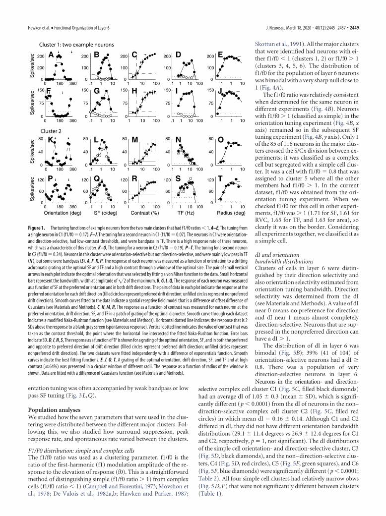
The first main cluster (C1: n � 15 of 116, 13%) was comprisedof highly responsive and highly sensitive, direction-selectivecomplex cells (two examples in Fig. 1A–E, F–J). One distinguish-ing parameter in the cluster analysis was the f1/f0 ratio. The f1/f0ratios of the two example neurons from the first main cluster

were 0.17 and 0.07, both in the lower quartile of ratios of complexcells. Another major distinguishing feature of the tuning of thefirst cluster was that all neurons were strongly direction-selective(Fig. 1A,F). Neurons in the first cluster often showed strongsuppression (below the spontaneous baseline shown by the hor-izontal dotted line) in the nonpreferred direction for a grating ofthe optimal orientation (e.g., Fig. 1F). Many of the neurons in C1also had relatively low contrast thresholds and saturating contrastresponse functions (Fig. 1C,H). In the TF domain, most of theneurons in C1 were strongly bandpass in TF tuning as exempli-fied in the two example neurons (Fig. 1D, I). In the experimentwhere the radius of the stimulus window was changed, someneurons in C1 showed a modest attenuation of their response atthe largest window sizes (Fig. 1E, J), although no parameter fromthis experiment was used in the cluster analysis.

The neurons in the second major cluster (C2: n � 20 of 116,17%) also had low f1/f0 ratios (0.19, 0.24 for the two examplesshown in the third and fourth rows of Fig. 1). The neurons in C2were orientation-selective but not direction-selective (Fig.1K,P), unlike those in C1. There were some neurons in C2 thatwere low pass in TF (Fig. 1N) and others that were bandpass (Fig.1S). Neurons in C2 showed very little size tuning (Fig. 1O,T).

The neurons in the other four major clusters (C3-C6) hadf1/f0 ratios �1, and therefore were classified as simple cells (Skot-tun et al., 1991). Ratios for the example neurons in C3 (Fig.2A–J), C4 (Fig. 2K–T), C5 (Fig. 3A–E), and C6 (Fig. 3F–J) were1.5, 1.1, 1.6, 1.5, 1.4, and 1.8, respectively. The example simplecells in C3 (n � 18 of 116, 16%) showed orientation selectivityand strong direction selectivity (Fig. 2A,F) that were character-istics of this cluster. The strong directional selectivity was ob-served across all spatial (Fig. 2B,G) and temporal (Fig. 2D, I)frequencies tested for the two example neurons. Another distin-guishing tuning characteristic of the third cluster is shown by thebandpass TF tuning of the two example neurons (Fig. 2D, I);bandpass TF tuning was also a common feature of this cluster.

The neurons in C4 (n � 15 of 116, 13%) were orientation-selective but not direction-selective (Fig. 2K,P). The lack of di-rection selectivity in C4 was evident in the spatial (Fig. 2L,Q) andtemporal (Fig. 2N,S) frequency tuning of the example neurons.The tuning shape for both spatial (Fig. 2L,Q) and temporal (Fig.2N,S) frequency along with the response amplitude was similarin both directions of movement at the preferred orientation. TheTF tuning of the two example neurons from cluster 4 were lowpass. This was a common but not universal feature of C4. Most ofthe neurons in clusters 3 and 4 showed little attenuation in theirresponse at large stimulus sizes as shown for the four exampleneurons (Fig. 2E, J,O,T).

One distinguishing feature of two additional clusters (C5, n �9; C6, n � 8) with f1/f0 ratios � 1 was their low sensitivity tocontrast as can be seen in the nonsaturating contrast responsefunctions from the two example neurons (Fig. 3C,H). Neurons inC5 and C6 were orientation-selective, and some were moderatelydirection-selective (Fig. 3A). However, they were distinguishedby their TF tuning: neurons in C5 were bandpass in TF (Fig. 3D),whereas those in C6 were low pass in TF (Fig. 3I).

The remaining clusters had few members (5 or fewer); there-fore, it was not possible to verify their uniqueness with the rela-tively small population sample. Two features separated mostmembers of these relatively small clusters from the six largerclusters. One was broad orientation tuning. Often neurons had apreferred orientation but also responded across all orientationswith a response at the orthogonal-to-preferred orientation (Fig.3K,P). The second distinguishing feature was that the broad ori-

Table 1. Orientation bandwidth

C1 C2 C3 C4 C5 C6

C1 1 7.0a 4.9a 5.1a 3.5a

29.1 � 11.4C2 p � 1 5.6a 3.5 3.9 1.326.9 � 12.4C3 p � 0.003a p � 0.01a 1 1 115.9 � 5.3C4 p � 0.03a p � 0.08 p � 1 1 117.5 � 9.1C5 p � 0.02a p � 0.06 p � 1 p � 1 115.4 � 4.5C6 p � 0.27 p � 0.76 p � 1 p � 1 p � 118.9 � 10.5

The values in the first column under the cluster number show the mean � SD for each cluster. The p values (belowthe diagonal) were all determined using a multiple comparison of the output of a one-way ANOVA using theBonferroni method to provide the adjustment to compensate for multiple comparisons. Values above the diagonalare 1 � log(p) indicating the full range of significance values.aValues reached significance level �0.05.

Table 2. Direction index

C1 C2 C3 C4 C5 C6

C1 39.9a 1 26.8a 19.1a 23.1a

1.05 � 0.30C2 p � 0.0001a 33.7a 2.2 2.8 10.16 � 0.14C3 p � 0.99 p � 0.0001a 20.1a 13.2a 17.4a

0.90 � 0.13C4 p � 0.0001a p � 0.31 p � 0.0001a 1 10.34 � 0.31C5 p � 0.0001a p � 0.17 p � 0.0001a p � 1 10.40 � 0.24C6 p � 0.0001a p � 1 p � 0.0001a p � 1 p � 10.28 � 0.20



entation tuning was often accompanied by weak bandpass or lowpass SF tuning (Fig. 3L,Q).

Population analysesWe studied how the seven parameters that were used in the clus-tering were distributed between the different major clusters. Fol-lowing this, we also studied how surround suppression, peakresponse rate, and spontaneous rate varied between the clusters.

F1/F0 distribution: simple and complex cellsThe f1/f0 ratio was used as a clustering parameter. f1/f0 is theratio of the first-harmonic (f1) modulation amplitude of the re-sponse to the elevation of response (f0). This is a straightforwardmethod of distinguishing simple (f1/f0 ratio � 1) from complexcells (f1/f0 ratio � 1) (Campbell and Fiorentini, 1973; Movshon etal., 1978; De Valois et al., 1982a,b; Hawken and Parker, 1987;

Skottun et al., 1991). All the major clustersthat were identified had neurons with ei-ther f1/f0 � 1 (clusters 1, 2) or f1/f0 � 1(clusters 3, 4, 5, 6). The distribution off1/f0 for the population of layer 6 neuronswas bimodal with a very sharp null close to1 (Fig. 4A).

The f1/f0 ratio was relatively consistentwhen determined for the same neuron indifferent experiments (Fig. 4B). Neuronswith f1/f0 � 1 (classified as simple) in theorientation tuning experiment (Fig. 4B, xaxis) remained so in the subsequent SFtuning experiment (Fig. 4B, y axis). Only 1of the 85 of 116 neurons in the major clus-ters crossed the S/Cx division between ex-periments; it was classified as a complexcell but segregated with a simple cell clus-ter. It was a cell with f1/f0 � 0.8 that wasassigned to cluster 5 where all the othermembers had f1/f0 � 1. In the currentdataset, f1/f0 was obtained from the ori-entation tuning experiment. When wechecked f1/f0 for this cell in other experi-ments, f1/f0 was � 1 (1.71 for SF, 1.61 forRVC, 1.65 for TF, and 1.63 for area), soclearly it was on the border. Consideringall experiments together, we classified it asa simple cell.

dI and orientationbandwidth distributionsClusters of cells in layer 6 were distin-guished by their direction selectivity andalso orientation selectivity estimated fromorientation tuning bandwidth. Directionselectivity was determined from the dI(see Materials and Methods). A value of dInear 0 means no preference for directionand dI near 1 means almost completelydirection-selective. Neurons that are sup-pressed in the nonpreferred direction canhave a dI � 1.

The distribution of dI in layer 6 wasbimodal (Fig. 5B); 39% (41 of 104) oforientation-selective neurons had a dI �0.8. There was a population of verydirection-selective neurons in layer 6.Neurons in the orientation- and direction-

selective complex cell cluster C1 (Fig. 5C, filled black diamonds)had an average dI of 1.05 � 0.3 (mean � SD), which is signifi-cantly different (p � 0.0001) from the dI of neurons in the non–direction-selective complex cell cluster C2 (Fig. 5C, filled redcircles) in which mean dI � 0.16 � 0.14. Although C1 and C2differed in dI, they did not have different orientation bandwidthdistributions (29.1 � 11.4 degrees vs 26.9 � 12.4 degrees for C1and C2, respectively, p � 1, not significant). The dI distributionsof the simple cell orientation- and direction-selective cluster, C3(Fig. 5D, black diamonds), and the non– direction-selective clus-ters, C4 (Fig. 5D, red circles), C5 (Fig. 5F, green squares), and C6(Fig. 5F, blue diamonds) were significantly different (p � 0.0001;Table 2). All four simple cell clusters had relatively narrow obws(Fig. 5D,F) that were not significantly different between clusters(Table 1).

F0 180 360

0

200

200

Spi

kes/

sec

.1 1 10 0

100

200

1 10 1000

100

200

.1 1 10 1000

100

200

.1 1 100

100

200

0 180 3600

75

150

Spi

kes/

sec

.1 1 10 0

75

150

1 10 1000

150

.1 1 10 1000

75

150

.1 1 100

75

150

0 180 3600

40

80

Spi

kes/

sec

.1 1 10 0

40

80

1 10 1000

40

80

.1 1 10 1000

40

80

.1 1 100

40

80

0 180 3600

60

120

Orientation (deg)

Spi

kes/

sec

.1 1 10 0

60

120

SF (c/deg)1 10 100

0

60

120

Contrast (%).1 1 10 100

0

60

120

TF (Hz).1 1 10

0

60

120

Radius (deg)

A B C D E

G H I J

K L M N O

P Q R S T

Cluster 1: two example neurons

Cluster 2

75

Figure 1. The tuning functions of example neurons from the two main clusters that had f1/f0 ratios � 1. A–E, The tuning froma single neuron in C1 (f1/f0 � 0.17). F–J, The tuning for a second neuron in C1 (f1/f0 � 0.07). The neurons in C1 were orientation-and direction-selective, had low-contrast thresholds, and were bandpass in TF. There is a high response rate of these neurons,which was a characteristic of this cluster. K–O, The tuning for a neuron in C2 (f1/f0 � 0.19). P–T, The tuning for a second neuronin C2 (f1/f0 � 0.24). Neurons in this cluster were orientation-selective but not direction-selective, and were mainly low pass in TF(N ), but some were bandpass (S). A, F, K, P, The response of each neuron was measured as a function of orientation to a driftingachromatic grating at the optimal SF and TF and a high contrast through a window of the optimal size. The pair of small verticalarrows in each plot indicate the optimal orientation that was selected by fitting a von Mises function to the data. Small horizontalbars represent the bandwidth, width at amplitude of 2 of the maximum. B, G, L, Q, The response of each neuron was measuredas a function of SF at the preferred orientation and in both drift directions. The pairs of data in each plot indicate the response at thepreferred orientation for each drift direction (filled circles represent preferred drift direction; unfilled circles represent nonpreferreddrift direction). Smooth curves fitted to the data indicate a spatial receptive field model that is a difference of offset difference ofGaussians (see Materials and Methods). C, H, M, R, The response as a function of contrast was measured for each neuron at thepreferred orientation, drift direction, SF, and TF in a patch of grating of the optimal diameter. Smooth curve through each datasetindicates a modified Naka-Rushton function (see Materials and Methods). Horizontal dotted line indicates the response that is 2SDs above the response to a blank gray screen (spontaneous response). Vertical dotted line indicates the value of contrast that wastaken as the contrast threshold, the point where the horizontal line intersected the fitted Naka-Rushton function. Error barsindicate SD. D, I, N, S, The response as a function of TF is shown for a grating of the optimal orientation, SF, and in both the preferredand opposite to preferred direction of drift direction (filled circles represent preferred drift direction; unfilled circles representnonpreferred drift direction). The two datasets were fitted independently with a difference of exponentials function. Smoothcurves indicate the best fitting functions. E, J, O, T, A grating of the optimal orientation, drift direction, SF, and TF and at highcontrast (�64%) was presented in a circular window of different radii. The response as a function of radius of the window isshown. Data are fitted with a difference of Gaussians function (see Materials and Methods).


Most neurons we studied in layer 6 hada measurable orientation bandwidth, al-though a small number (n � 12 of 116,10%) were nonoriented (Fig. 5A). Thedistribution of orientation bandwidth forall orientation-selective neurons in layer 6had a median value of 20.5 deg. (Fig. 5A).Although, when comparing within thesame f1/f0 clusters, there were no signifi-cant differences in orientation band-width, there were significant differencesbetween C1 and C3–C5 and between C2and C3 (for p values, see Table 1).

In the population analyses, we showdata for the smaller clusters in the figuresbut do not compare their tuning with thelarger clusters in the statistical compari-sons (Tables 1-8). The smaller clusters areshown for completeness. We combined 3small clusters with f1/f0 � 1 and 2 � N �9 as solid green symbols for visualization,and show 1 cluster with f1/f0 � 1, N � 4 assolid blue symbols (Fig. 5D). The 3 clus-ters with f1/f0 � 1 and 2 � N � 9 areshown as cyan crosses, purple crosses, andcyan triangles (Fig. 5G). Qualitatively, thecluster with f1/f0 � 1 had dIs of �2 (Fig.5E, blue filled triangles); these were dis-tinct from all the other neurons as theyhad relatively high maintained rates andshowed a large suppression in the oppo-site to preferred direction. Other neuronswith f1/f0 � 1 that were in the minor clus-ters were relatively untuned for orienta-tion as in the example neurons in Figure3K, P and accounted for some neurons inthe smaller clusters (Fig. 5G).

SF tuningOne of the characteristic features of manycortical receptive fields is that they havemultiple subunits (Hubel and Wiesel,1962, 1968) that can result in relativelynarrow SF tuning of neurons (Movshon etal., 1978; De Valois et al., 1982a; Hawkenand Parker, 1987). We measured the SFtuning at the preferred orientation, driftdirection, and TF for high-contrast grat-ings (�64% contrast) and determined thebandwidth from the difference of offsetdifference of Gaussians function fitted tothe response data (see Materials andMethods). All but two of the neurons inC1 were bandpass in SF (Fig. 6A, blackdiamonds); the population had meanbandwidth of 2.4 � 1.2 octaves (mean �SD) and was not significantly different (Table3) from the bandwidth distribution ofneurons in C2 (2.9 � 1.3 octaves, mean �SD) where two neurons were low pass(Fig. 6A, red filled circles). All the neuronsin the other four major clusters werebandpass in SF (Fig. 6B, black unfilled di-

0 180 3600

45

Spi

kes/

sec

1 10 1000

45

90

.1 1 10 1000

45

90

.1 1 100

45

90

0 180 3600

20

40

Spi

kes/

sec

.1 1 10 0

20

40

1 10 1000

20

40

.1 1 10 1000

20

40

.1 1 100

20

40

0 180 3600

15

Spi

kes/

sec

.1 1 10 0

15

1 10 1000

15

.1 1 10 1000

15

.1 1 100

15

0 180 3600

30

60

Orientation (deg)

Spi

kes/

sec

.1 1 10 0

30

60

SF (c/deg)1 10 100

0

30

60

Contrast (%).1 1 10 100

0

30

60

TF (Hz).1 1 10

0

30

60

Radius (deg)

.1 1 10 0

45

90A B C D E

F G H I J

P Q R S T

Cluster 390

30 30 303030 K L M N OCluster 4

Figure 2. The tuning functions of example neurons from two of the four main clusters that had f1/f0 ratios � 1. A–E, F–J,Tuning of two example neurons from C3 (f1/f0 1.5 and 1.1, respectively). These neurons, characteristic of the cluster, were stronglydirection-selective and bandpass in TF. K–O, P–T, Tuning functions of two example neurons from C4 (f1/f0 1.6 and 1.7, respec-tively). These neurons were orientation-selective but not direction-selective with low pass TF tuning. The other details are as forFigure 1.

0 180 3600

25

50

Spi

kes/

sec

.1 1 10 0

25

50

1 10 1000

25

50

.1 1 10 1000

25

50

.1 1 100

25

50

0 180 3600

15

30

Spi

kes/

sec

.1 1 10 0

15

30

1 10 1000

15

30

.1 1 10 1000

15

30

.1 1 100

15

30

0 180 3600

25

50

Spi

kes/

sec

.1 1 10 0

25

50

1 10 1000

.1 1 10 1000

25

50

.1 1 100

25

50

0 180 3600

25

50

Orientation (deg.)

Spi

kes/

sec

.1 1 10 0

25

50

SF (c/deg)

1 10 1000

25

50

.1 1 10 1000

25

50

TF (Hz)

.1 1 100

25

50

Radius (deg)

A B C D E

F G H I J

K L M N O

P Q R S T

25

50

Cluster 5

Other Clusters

Cluster 6

Contrast (%)

Figure 3. A–E, F–J, The tuning functions of example neurons from C5 and C6. The neurons in these clusters were orientationand SF selective, but one characteristic that separated them from the other two clusters was their insensitivity to contrast. They areseparated from each other by their TF tuning, neurons in C5 were bandpass, and those in C6 were low pass. K–O, P–T, Neuronsfrom the smaller clusters where most of the neurons were weakly selective for orientation and relatively low pass in SF (f1/f0 1.3and 1.5, respectively). The other details are as for Figure 1.


amonds, C3; red unfilled circles, C4; Fig. 6D, green unfilledsquares, C5 and blue triangles, C6). None of their SF bandwidthdistributions were significantly different (Table 3). The SF band-width distribution of C6 was significantly narrower than the dis-tribution from both C1 and C2, whereas the distributions fromC3, C4, and C5 were narrower than C2 (Table 3). Some of theneurons in the smaller clusters were low pass (Fig. 6C,E), whereasothers were bandpass (Fig. 6C, blue diamonds, E, magentacrosses).

TF tuningPrevious studies have shown that there is a range of TF tuning inV1. However, there has not been a systematic analysis at the level

of single cortical layers. In the examplesfrom the different layer 6 clusters, someneurons were strongly bandpass in TF(Figs. 1D, I, 2D, I, 3D), whereas otherneurons were low pass in TF (Figs. 1N,2N,S, 3I). We used TF bandwidth toquantify the width of the tuning and thedegree of attenuation at low temporal fre-quencies. The high- and low-frequencyhalf-height points were determined foreach neuron from the fit of a difference ofexponentials to the data (see Materialsand Methods). If a fit did not attenuate tohalf-amplitude by a TF of 0.1, we assignedthe low TF half-height point � 0.1, thenused this point and the high frequencyat half-amplitude to determine band-width. A number of neurons with no orweak and shallow low-frequency attenua-tion would have a slightly narrower band-width than their true bandwidth using thisassignment, but we used it to allow us tomake quantitative comparisons of the dif-ferent clusters. Neurons with bandwidths �6 are shown as low pass (lp) in Figure 7.

Neurons in the main direction-selective complex cell cluster (C1) werepredominantly bandpass in TF (Fig. 7A,black filled diamonds), whereas the ma-jority of the non– direction-selective com-plex cell cluster (C2) were mostly low passin their TF tuning (Fig. 7A, red filled cir-cles). The mean bandwidths of the twomain complex cell clusters C1 and C2were significantly different (3.6 � 1.9 vs5.4 � 1.6, p � 0.005; Table 4). There alsowas a clear separation in the TF band-widths of the neurons in the two largestsimple cell clusters C3 and C4 (Fig. 7B,black unfilled diamonds and red unfilledcircles). Neurons in the direction-selective cluster (C3) were all bandpass inTF, whereas neurons in the non–direction-selective cluster (C4) werenearly all low pass; the difference betweenthese two clusters was significant (p �0.0001; Table 4), as was the difference be-tween C4 and C5 ( p � 0.0001). How-ever, TF bandwidth distributions of C4and C6 were predominantly low pass(Fig. 7B, red circles, D, blue triangles)

and not significantly different (Table 4). C5 and C6 hadsignificantly different TF bandwidth distributions (Fig. 7D;Table 4).

Contrast response distributions: threshold and c50Each neuron’s response as a function of contrast for gratings ofoptimal orientation, direction, and spatial and TF was fit with amodified Naka-Rushton function (Peirce, 2007) (see Materialsand Methods). Two measures of the response were obtained fromthe fitted functions and used as parameters in the clustering: (1)the contrast at which the response reached half its maximum(c50); and (2) the contrast threshold (cTh), defined as the contrast

0 1 20

20

40

f1/f0 ratio

Num

ber

of N

euro

ns

0 1 2

0

1

2

f1/f0 ratio from ORIf1

/f0 r

atio

from

SF

A B

C1C2C3C4C5C6

Figure 4. A, The distribution of f1/f0 ratio for all the neurons in the sample from layer 6 (n � 116). The f1/f0 ratio was used asone of the response measures in the clustering procedure. B, The f1/f0 ratio measured in the orientation tuning experiment (x axis)plotted against the f1/f0 ratio of the same cell measured from the SF tuning experiment (y axis). Symbols represent clusterassignments. There were six main clusters that are shown as filled black diamonds (C1), filled red circles (C2), unfilled blackdiamonds (C3), unfilled red circles (C4), unfilled green squares (C5), and unfilled blue triangles (C6). Unfilled magenta triangles andcyan and magenta crosses represent three smaller clusters with f1/f0 ratios � 1. Filled blue triangles represent a small cluster withf1/f0 � 1. Filled green squares represent four further clusters with f1/f0 � 1 and with � 4 neurons that were combined. Theclusters were clearly separated according to whether they are complex (f1/f0 � 1) or simple (f1/f0 � 1).

0 25 500

20

40

# N

euro

ns

Ori BW (deg)0 .5 1

0

20

40

Direction Index0 25 50

0

.5

1

Dire

ctio

n In

dex

0 25 50 0

.5

1

0 25 50 0

1

2

Ori BW (deg)

Dire

ctio

n In

dex

0 25 50 0

.5

1

0 25 50

0

.5

1

Ori BW (deg)

A B C D

FE G

no no

no no no

no

Ori BW (deg)

C1C2C3C4C5C6

Figure 5. Orientation bandwidth (obw) and dI were two tuning parameters used in the clustering procedure. A, The distributionof obw for the whole layer 6 sample. no, Nonoriented. B, The distribution of dI for the whole sample. C–G, The relationshipbetween obw (x axis) and dI (y axis) for the same clusters shown in Figure 4. C, The obw/dI relationship for C1 (filled blackdiamonds) and C2 (filled red circles). There is a clear separation by dI but not obw in the two clusters. D, The relationship for C3(unfilled black diamonds) and C4 (unfilled red circles). There is a clear separation based on dI but not obw in the two clusters. E, Theobw/dI relationship between the remaining clusters where the clusters also had f1/f0 � 1. The neurons in the small cluster (filledblue triangles) are very direction-selective and strongly suppressed in the nonpreferred direction. Filled green squares representthe combination of three small clusters. F, The obw/dI relationship for C5 (green squares) and C6 (blue triangles), both withneurons that have f1/f0 � 1. G, Three small clusters (unfilled cyan triangles, magenta crosses, and cyan crosses) where all theclusters also had f1/f0 � 1.


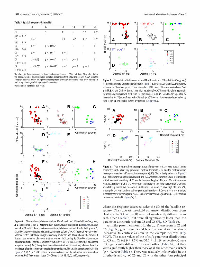
where the response exceeded twice the SD of the baseline re-sponse. The contrast threshold parameter distributions fromclusters C1–C4 (Fig. 8A,B) were not significantly different fromeach other (Table 5) but were all significantly lower than theparameter distributions from C5 and C6 (Fig. 8D; Table 5).

A similar pattern was found for the c50. The neurons in C5 andC6 (Fig. 8D, green squares and blue diamonds) were relativelyinsensitive to contrast as seen in the example neurons (Fig.3C,H). The mean values of the of c50’s parameter distributionsfor C5 and C6 (48.9 � 8.2% and 52.2 � 11.1%, respectively) werenot significantly different from each other (Table 6), but theywere significantly higher than those of all the other main clusters(p � 0.0001; Table 6). There was relatively little overlap in thethresholds and c50 of C5 and C6 with the other four principal

.1 1 100

2

4

SF

ban

dwid

th (

octa

ves)

.1 1 100

2

4

.1 1 100

2

4

.1 1 100

2

4

.1 1 100

2

4

Optimal SF (c/deg)

lp lp

lp lp

lpA B C

D E

C1C2C3C4C5C6

Optimal SF (c/deg)

.1 1 10.1

1

10

.1 1 10.1

1

10

.1 1 10.1

1

10

.1 1 10.1

1

10

.1 1 10.1

1

10

Opt

imal

rad

ius

(de

g)

I J

Optimal SF (c/deg)

Optimal SF (c/deg)

F G H

Figure 6. The relationship between optimal SF (osf, x axis) and SF bandwidth (sfbw, y axis,A–E) and optimal radius (F–J ) for the main clusters. Cluster designation as in Figure 5. lp, Lowpass. A, In C1 and C2, there is an inverse relationship between osf and sfbw for both groups. B,C3 and C4 show overlapping relationships between osf and sfbw. C, The small very direction-selective clusters (filled blue triangles) have very similar osfs and sfbws, whereas the combinedclusters have a number of neurons that are low pass in SF tuning. D, C5 and C6 show narrowsfbws across a range of osfs. E, Neurons in two clusters are low pass in SF; the other is bandpass(magenta crosses). F–J, The optimal summation radius for C1 is restricted, whereas there is abroad span of optimal summation radius for other clusters. The smaller clusters are detailed inFigure 5C, E, H, J. For 5 of 85 cells in the 6 main clusters, we did not obtain area summationmeasures. F–J, The n in each cluster C1–C6 was 15, 20, 18, 13, 7, and 7, respectively.

1 10 0

2

4

TF

BW

(oc

tave

s)

1 10 0

2

4

Optimal TF (Hz)

1 10 0

2

4

1 10 0

2

4

1 10 0

2

4

Optimal TF (Hz)

A B C

D E

lp lp

lp lp

lp

C1C2C3C4C5C6

Figure 7. The relationship between optimal TF (otf, x axis) and TF bandwidth (tfbw, y axis)for the main clusters. Cluster designation as in Figure 5. lp, Low pass. A, C1 and C2, the majorityof neurons in C1 are bandpass in TF and have otfs �10 Hz. Many of the neurons in cluster 2 arelp in TF. B, C3 and C4 show distinct separation based on tfbw. C, The majority of the neurons inthe remaining clusters with f1/f0 ratio � 1 are low pass in TF. D, C5 and C6 are separated bytheir tuning for TF (except 1 neuron in C5 that is lp). E, Three small clusters are distinguished bytheir TF tuning. The smaller clusters are detailed in Figure 5C, E.

1 10 100 1

10

100

Contrast Threshold (%)

C50

(%

)

1 10 100 1

10

100

1 10 100 1

10

100

1 10 100 1

10

100


B C

D E1 10 100

1

10

100

C50

(%

)

A

C1C2C3C4C5C6


Figure 8. Two measures from the response as a function of contrast were used as tuningparameters in the clustering procedure: contrast threshold (cTh) and the contrast wherethe response reached half the maximum response (c50). Cluster designation as in Figure 5.A, C1 has neurons with relatively low cTh and c50, whereas neurons in C2 are intermediatein their contrast sensitivity. B, C3 and C4 have overlapping cThs and c50s but are some-what less sensitive than C1. C, Neurons in the direction-selective cluster (blue triangles)are relatively insensitive to contrast. D, Neurons in C5 and C6 have high cThs and c50,making the clusters stand out as being contrast insensitive. E, One cluster is intermediatein contrast sensitivity (magenta crosses), another insensitive (cyan triangles). The smallerclusters are detailed in Figure 5C, E.

Table 3. Spatial frequency bandwidth

C1 C2 C3 C4 C5 C6

C1 1 1 1 3.0 4.2a

2.36 � 1.19C2 p � 1 6.3a 5.7a 8.5a 9.7a

2.93 � 1.29C3 p � 1 p � 0.005a 1 1 11.80 � 0.64C4 p � 1 p � 0.01a p � 1 1 11.79 � 0.78C5 p � 0.13 p � 0.001a p � 1 p � 1 11.30 � 0.34C6 p � 0.05a p � 0.0005a p � 1 p � 1 p � 11.10 � 0.32

The values in the first column under the cluster number show the mean � SD for each cluster. The p values (belowthe diagonal) were all determined using a multiple comparison of the output of a one-way ANOVA using theBonferroni method to provide the adjustment to compensate for multiple comparisons. Values above the diagonalare 1 � log indicating the full range of significance values.aValues reached significance level �0.05.


clusters. Among the other four clusters, only the c50 parameterdistribution for C3 was significantly higher than for C1 (Table 6).The smaller simple cell clusters had restricted ranges of c50 andcTh values (Fig. 8E) within the clusters but were within the rangeof values in the major clusters.

Area tuning distributionsMost neurons in our sample summed visually evoked signals asstimulus size increased until a maximal area (Figs. 1–3E, J,O,T)and then maintained a plateau, with a small amount of suppres-sion at the largest areas for a few neurons. There was a relativelybroad distribution of optimal radius within the most of the majorclusters (Fig. 6F–J), although C1 showed a narrower range, prob-ably due to the small degree of surround suppression. Areal sum-mation with weak or no surround suppression is characteristic oflayer 6 neurons’ receptive fields (Schiller et al., 1976a; Gilbert,

Table 4. Temporal frequency bandwidth

C1 C2 C3 C4 C5 C6

C1 7.4a 3.8 14.2a 1.6 10.8a

3.62 � 1.89C2 p � 0.005a 21.5a 1.6 13.7a 1.15.42 � 1.61C3 p � 0.06 p � 0.0001a 28.4a 1 21.8a

2.28 � 0.71C4 p � 0.0001a p � 0.52 p � 0.0001a 20.0a 16.38 � 0.33C5 p � 0.54 p � 0.0001a p � 1 p � 0.0001a 16.4a

2.46 � 1.71C6 p � 0.001a p � 0.95 p � 0.0001a p � 1 p � 0.0001a

6.45 � 0.13


Table 5. Contrast threshold

C1 C2 C3 C4 C5 C6

C1 1 1 1 19.9a 31.9a

4.3 � 2.9C2 p � 1 1 1 15.0a 27.5a

7.1 � 3.7C3 p � 1 p � 1 1 15.7a 28.0a

6.6 � 4.2C4 p � 1 p � 1 p � 1 18.9a 31.0a

4.7 � 2.4C5 p � 0.0001a p � 0.0001a p � 0.0001a p � 0.0001a 2.918.2 � 6.8C6 p � 0.0001a p � 0.0001a p � 0.0001a p � 0.0001a p � 0.1524.2 � 8.9


Table 6. c50 contrast

C1 C2 C3 C4 C5 C6

C1 3.1 7.4a 2.8 39.4a 41.4a

8.5 � 4.4C2 p � 0.13 1 1 31.8a 34.2a

16.2 � 7.4C3 p � 0.005a p � 1 1 25.5a 28.2a

20.4 � 10.8C4 p � 0.18 p � 1 p � 1 29.5a 31.9a

16.4 � 7.5C5 p � 0.0001a p � 0.0001a p � 0.0001a p � 0.0001a 148.9 � 8.2C6 p � 0.0001a p � 0.0001a p � 0.0001a p � 0.0001a p � 152.2 � 11.1


Table 7. Peak firing rate

C1 C2 C3 C4 C5 C6

C1 12.3a 13.2a 12.3a 10.5a 9.9a

140 � 43C2 p � 0.0001a 3.7 5.7 7.8 8.552 � 19C3 p � 0.0001a p � 1 2.5 4.8 5.637 � 16C4 p � 0.0001a p � 0.38 p � 1 3.1 3.029 � 14C5 p � 0.0001a p � 0.07 p � 1 p � 1 1.219 � 9C6 p � 0.0001a p � 0.06 p � 1 p � 0.14 p � 0.8518 � 7

The values in the first column under the cluster number show the mean � SD for each cluster. The p values were alldetermined using Kruskal–Wallis nonparametric test.aValues reached significance level �0.05.

Table 8. Spontaneous firing rate

C1 C2 C3 C4 C5 C6

C1 3.6 15.1a 13.3a 10.5a 10.1a

14.0 � 7.3C2 p � 0.07 16.2a 13.4a 10.7a 10.7a

9.0 � 6.3C3 p � 0.0001a p � 0.0001a 2.6 2.4 2.10.10 � 0.20C4 p � 0.0001a p � 0.0001a p � 0.20 1.1 1.20.51 � 1.53C5 p � 0.0001a p � 0.0001a p � 0.24 p � 0.88 1.20.36 � 0.82C6 p � 0.0001a p � 0.0001a p � 0.32 p � 0.79 p � 0.850.09 � 0.14

The values in the first column under the cluster number show the mean � SD for each cluster. The p values were alldetermined using Kruskal–Wallis nonparametric test.aValues reached significance level �0.05.

Table 9. Area suppression index

C1 C2 C3 C4 C5 C6

C1 5.0a 7.1a 6.4a 5.1a 4.3a

0.38 � 0.22C2 p � 0.025a 1.3 1.2 1.0 1.10.14 � 0.18C3 p � 0.025a p � 0.73 1.0 1.2 1.30.11 � 0.24C4 p � 0.005a p � 0.78 p � 0.96 1.2 1.20.12 � 0.22C5 p � 0.025a p � 0.99 p � 0.80 p � 0.83 1.10.14 � 0.16C6 p � 0.05a p � 0.92 p � 0.77 p � 0.79 p � 0.950.14 � 0.25

The values in the first column under the cluster number show the mean � SD for each cluster. The p values weredetermined using Student’s t test. For 5 of 85 cells in the 6 main clusters, we did not obtain area summationmeasures. The n in each cluster C1-C6 was 15, 20, 18, 13, 7, and 7, respectively.aValues reached significance level �0.05.


1977). The only cluster that showed a consistent pattern of sup-pression, albeit relatively weak (mean SI � 0.38 � 0.22; Table 9),at the largest diameters was C1. The suppression observed in C1neurons was significantly greater than in all the other clusters(Table 9). In the area measurements, the maximum stimulusradius tested was 4 or 5 degrees for the majority of neurons.Therefore, if there were additional attenuation beyond this spa-tial extent caused by surround suppression, it would not havebeen measured. As a consequence, suppression may have beenunderestimated if it extended beyond a radius of 5 degrees.

Response rate and spontaneous rateSeven functional tuning properties were extracted and z-trans-formed for the clustering, but there were other tuning measuresand functional response properties that were not used. A numberof these are particularly notable because they tended to distributeaccording to cluster, even though they were not included in theclustering analysis.

Consider maximum spike rate. Across the six main clusters,there were mean maximum rates ranging from 140 spikes/s downto 18 spikes/s. The two main clusters accounting for the complexcell population (f1/f0 � 1) had clearly different ranges of peakfiring rates. In the direction-selective complex cell cluster (C1),the mean rate was 140 � 43 spikes/s (Fig. 9A), which was signif-icantly different from the mean rate of 52 � 19 spikes/s (Fig. 9C)in cluster C2 (p � 0.0001; Table 7).

The remaining four major clusters were predominantly sim-ple cells. The larger two of these clusters (C3 and C4) had meanmaximum spike rates 37 � 16 and 29 � 14 spikes/s, respectively,which were not significantly different (p � 0.26), whereas the twosmaller clusters, C5 and C6, had mean peak rates of 19 � 9 and18 � 7 spikes/s, respectively (compare Table 7).

It is well established that spontaneous firing rate differs be-tween simple and complex cell populations in the infragranularlayers of macaque V1 (Schiller et al., 1976a,b; Ringach et al.,2002). We determined that this was the case for the layer 6 pop-ulation (Fig. 10). The mean spontaneous rate for all neurons withf1/f0 ratios � 1 (complex cells) was 11.2 � 8.2 spikes/s, whereasthe mean rate for all neurons with f1/f0 ratios � 1 (simple cells)was 1.2 � 3.7 spikes/s. These distributions were significantly dif-ferent (p � 0.0001). C1 had the highest spontaneous rate (14 �7.3 spikes/s). C1’s spontaneous rate was not significantly differ-ent from the rate of C2 (9 � 6.3 spikes/s; Table 8). Of the overallpopulation of neurons with f1/f0 ratios � 1, the four major sim-ple cell clusters (C3-C6) all had similar ranges of f1/f0 and alsohad low mean spontaneous rates, all �1 spike/s (Table 8) that didnot differ between the clusters.

Relative depth of clusters within layer 6We determined whether the position of the recorded neuronswithin each cluster was distributed evenly across the depth oflayer 6 or whether there was any localization within the layer. Thisanalysis was done by ordering the neurons in each cluster accord-ing to their relative depth within layer 6, and then comparing theresulting profile with the profile of the total population. Theneurons in C1 were all found in the upper half of the layer as canbe seen by comparing the black diamonds (C1) with the smallblue circles (total population) in Figure 11A. In contrast, theneurons in C2 (Fig. 11A, red circles) were distributed through thedepth of the layer. There did not appear to be any major aggre-gation of neurons in the other main clusters (C3–C6) in the upperor lower regions of layer 6 (Fig. 11B).

DiscussionCluster analysis resultsOf the seven tuning features used for cluster analysis, three mea-sures were particularly useful for distinguishing the six majorfunctional clusters in layer 6: modulation ratio (f1/f0), direc-tional selectivity, and TF tuning.

The neurons in two of the six major clusters (C1 and C2) hadf1/f0 ratios � 1 and would be classified as complex cells (Skottunet al., 1991). Neurons in the other four clusters (C3–C6) had f1/f0ratios � 1 and would be classified as simple cells.

A second feature defining the clusters was direction selectivity.There were two major clusters, C1 and C3, that had neurons that

10 30 100 300 0

.2

.4

10 30 100 300 0

.2

.4

Pro

port

ion

Neu

rons

10 30 100 300 0

.2

.4

10 30 100 300 0

.2

.4

10 30 100 300 0

.2

.4

10 30 100 300 0

.2

.4

10 30 100 300 0

.2

.4

.6

10 30 100 300 0

.2

.4

Peak Rate (spikes/sec)

A B

C D

E F

G H

Figure 9. Distribution of maximum firing rates (see Materials and Methods) to optimalstimuli in each cluster. A, C, E, G, The distributions of peak firing rate of neurons in C1, C2, C6, andC7, respectively, all that had f1/f0 ratios � 1. Many neurons in C1 have high maximum firingrates. B, D, F, H, The distributions of peak firing rate of neurons in C3, C4, C5, and C6 respectively,all had f1/f0 ratios � 1.

C1C2C3C4C5C6

0 1 2.1

1

10

100

Modulation Ratio (f1/f0)

Spo

ntan

eous

Rat

e (s

pike

s/se

c)

Figure 10. Distribution of spontaneous firing rates (y axis) as a function of f1/f0 ratio (x axis)for all neurons shown as clusters in Figure 4. Neurons with spontaneous rate of �0.1 are shownas 0.1. There are two main groups: those with f1/f0 � 1 have spontaneous rates � 1, and thosewith f1/f0 � 1 have low spontaneous rate. Clusters as in Figure 4. The smaller clusters detailedin the Figure 5 legend are shown with the same symbols used in Figure 5.


were strongly direction-selective (Fig. 5A,B, filled and unfilledblack diamonds).

A third tuning measure, TF bandwidth, was also important indistinguishing C1 and C3 from the non– direction-selective com-plex and simple cell clusters. C1 and C3 were bandpass in TF(Figs. 7A,B, 12, filled and unfilled black diamonds). Three of theremaining four major clusters (C2, C4, and C6) were either com-plex or simple (Figs. 4B, 12), but they were non– direction-selective (Figs. 5A,B, 12) and mostly low pass in TF (Figs. 7A,B,12).

Tuning and response measures not used in thecluster analysisAlthough we did not use firing rate as a parameter for clustering,we showed (in Results) that visually driven firing rate was muchhigher in C1 than in C2, and both clusters C1 and C2 had higheraverage firing rates than in the simple cell clusters C3-C6. Simi-larly, spontaneous firing rate was significantly higher in C1 andC2 than in C3-C6, and the separation between complex and sim-ple cells within layer 6 (Fig. 10) was even more evident than theseparation in the overall V1 population (Ringach et al., 2002).Furthermore, the distribution of cells in depth was different forC1 from that of all the other clusters (Fig. 11).

Properties and possible functions of neurons in differentlayer 6 clustersCluster 1The visually evoked mean rate was 140 spikes/s for C1 neurons,and they did not appear to adapt, much like the rates of PVinhibitory interneurons (Rudy and McBain, 2001). The non-adapting high spike rate of the PV inhibitory interneurons isattributed to the expression of the Kv3.1b potassium channel

(Rudy and McBain, 2001). In rodents, the Kv3.1b channel is notexpressed in excitatory neurons in cortex. However, it is ex-pressed in some excitatory neurons in primate cortex (Constanti-nople et al., 2009; Kelly et al., 2019), and it is clearly expressed inthe large Meynert cells located near the layer 5/6 border in mon-key visual cortex (Ichinohe et al., 2004; Constantinople et al.,2009; Kelly et al., 2019). It is tempting to speculate that some ofthe high firing rate neurons in C1 are large pyramidal neuronsthat express Kv3.1b. All neurons in C1 were located in the top halfof the layer, layer 6a (Fig. 11). Because Meynert cells are sparse, itis unlikely that all the neurons in C1 are Meynert cells.

Neurons in C1 were very direction-selective (Figs. 5C, 12). Ithas been established that most Meynert cells project to extrastri-ate visual area MT (Fries et al., 1985; Nhan and Callaway, 2012),which contains many direction-selective neurons (Zeki, 1974).Further, some of the tuning characteristics of the neurons in C1,such as strong directionality, low contrast threshold (Fig. 8A),and saturating contrast response functions (Fig. 1C,H), matchthose of the neurons described by Movshon and Newsome (1996)that were recorded in layer 6 of macaque V1 and that were acti-vated antidromically by electrical stimulation of MT. The neu-rons in C1 showed some response attenuation at large stimuluswindow diameters (Fig. 1E, J) indicative of eCRF suppression.Their eCRF suppression may be inherited from magnocellularLGN neurons because M-pathway retinal ganglion cells (pre-sumptive parasol cells) show moderate eCRF suppression (Solo-mon et al., 2006). If some of the C1 population are also providinginput to MT, it is consistent with the findings that the functionalcharacteristics of the input to MT neurons are derived mainly viaV1, V2, and V3 through the M-pathway (Gegenfurtner et al.,1994).

Cluster 2Neurons in C2 were also complex cells (f1/f0 ratio � 1) but werenot direction-selective (Fig. 1K,P). However, all C2 neurons

0 .5 1 1

.5

0

Rel

ativ

e D

epth

0 .5 1 1

.5

0

Proportion Neurons

Rel

ativ

e D

epth

C1

C2

C3C4C5C6

A

B

Figure 11. The relative depth of each neuron is shown in serial order from top of layer 6. Eachcluster is shown by the same symbols as used in Figure 4 and subsequent figures. A, The relativedepth for C1 (black diamonds) shows that the neurons are found in the upper half of layer 6.Neurons in C2 (red circles) are distributed through the full depth of layer 6. Small blue circlesrepresent the serial order of the total sample of 116 neurons. B, The four clusters with f1/f0ratios � 1, C3–C6, are distributed through the full depth of layer 6.

0

3

6 lp

0

1

2 0

1

2

TF BW (octaves)

Direction Index

Mod

ulat

ion

Inde

x (f

1/f0

rat

io)

C1C2C3C4C5C6

Figure 12. Distribution of the six largest clusters is shown with respect to three tuningparameters: TF bandwidth (x axis), f1/f0 ratio (y axis), and dI (z axis). Each cluster is indicated bythe symbols described in Figure 4.


were orientation- and SF-selective (Fig. 1L,Q). The mean spikerate of the neurons in C2 was significantly lower than the meanrate in C1 (Table 7). As a cluster, they had higher average cTh andc50 values than C1 (Fig. 8; Tables 5, 6), but the differences werenot significant. Sixty-five percent of the neurons in C2 were lowpass in TF (13 of 20; Fig. 1N), and the majority showed little eCRFsuppression: the mean SI was 0.2, but there were two neurons thathad SI � 0.7. In distinction to the neurons in C1, this group ofneurons would provide signals about stationary or slowly movingborders.

Cluster 3All the neurons in C3 were simple cells (f1/f0 ratio � 1, mean �1.5) that were direction-, orientation-, and SF-selective and oftenstrongly bandpass in TF (Fig. 2A–J). The average orientationbandwidth was 16 degrees (Fig. 5D; Table 1), showing the nar-rowest average tuning of all the clusters. The neurons in C3 alsohad narrow TF bandwidths (mean 2.3 octaves; Table 4) but arange of optimal TFs (Fig. 7B). The combination of narrow tun-ing for TF, but a range of optimal TFs and a range of optimal SFs(Fig. 6B), suggests that this population of simple cells may span aselective range of velocity preferences. This cluster of neuronswould signal the sign and direction of movement of objects andedges over all but the lowest contrast range.

Cluster 4The neurons in C4 were distinguished from those of C3 by theirlack of direction selectivity (Figs. 2K,L,N,P,Q,S, Fig. 5D) andtheir low pass TF tuning (Fig. 7B; Table 4). The cluster had asimilar range of contrast threshold and c50 to C3. The averagepeak firing rate of neurons in C4 was not significantly differentfrom the rate in C3 (Table 7). The neurons in C4 were signifi-cantly more sensitive to contrast than those in C5 and C6 (Tables5, 6). This cluster of neurons, because they are simple cells and arelow pass in TF, are the only cluster that would signal the sign andlocation of oriented edges in an image across a range of sizes atlow and intermediate contrasts in a stationary achromatic image.

Clusters 5 and 6Most neurons in C5 and C6 were characterized by relatively nar-row orientation and SF bandwidth combined with low sensitivityto achromatic contrast. It has been a longstanding mystery howthe visual system maintains a high level of contrast discrimina-tion for achromatic stimuli over a wide range of base contrasts(Legge, 1981; Barlow et al., 1987; Chirimuuta and Tolhurst,2005a,b). The parcellation of neurons into clusters with differentdynamic ranges for different contrast ranges suggests a solutionto this long-standing puzzle of contrast discrimination and iden-tification (Chirimuuta and Tolhurst, 2005a,b). Clusters C5 andC6 were distinguished from each other by their TF selectivity.Almost all neurons in C5 were bandpass for TF (Fig. 7D, greensquares), whereas those in C6 were low pass for TF (Fig. 7D, bluetriangles). Both clusters were distributed through the depth oflayer 6 (Fig. 11B).

Minor clustersSome of the smaller clusters had neurons that were relativelyuntuned for orientation and low pass in SF (Figs. 3K,L,P,Q,5E,G, 6C,E). These are properties that have been attributed toinhibitory interneurons (Nowak et al., 2008), but anatomicalidentification along with functional characterization is necessaryto show that these neurons are inhibitory. Validation of theseminor clusters would require an even larger sample of recordedlayer 6 neurons.

Implications of clustersIf the functional subpopulations described in the current studyare related to the structurally defined subclasses in layer 6 (Wiserand Callaway, 1996; Hasse et al., 2019), then there will be separatetarget regions for the axons of these neurons. The diversity offunctional types may be related to the function of their targetsites. Many layer 6 neurons project intracortically (Wiser andCallaway, 1996), and some have axons preferentially terminatingin layer 4C�, the major M-pathway recipient sublayer in V1,whereas others that preferentially arborize in layer 4C� and layer4A, the principal P-pathway recipient zones of layer 4. Althoughit is currently not known how these anatomical subclasses maponto our functionally defined clusters, if functional selectivitymaps to anatomical classes, L6 neurons in different functionalclusters could provide cluster-specific feedback. Approximately10%–15% of layer 6 neurons provide feedback projections to theLGN (Fitzpatrick et al., 1994), and these have some functionalattributes (Briggs and Usrey, 2009; Hasse and Briggs, 2017) thatalign mainly with two of the clusters (C2 and C6) we have iden-tified. Another structurally defined group of neurons project toextrastriate visual area MT (Lund et al., 1975; Fries et al., 1985;Nhan and Callaway, 2012). Movshon and Newsome (1996)showed that some layer 6 neurons projecting to MT have func-tional properties similar to those of C1. Future studies combiningfunctional and anatomical characterization may reveal whetherthese functional clusters indeed correspond to particular ana-tomical classes.

ReferencesBarlow HB, Kaushal TP, Hawken M, Parker AJ (1987) Human contrast dis-

crimination and the threshold of cortical neurons. J Opt Soc Am A4:2366 –2371.

Bonds AB (1991) Temporal dynamics of contrast gain in single cells of thecat striate cortex. Vis Neurosci 6:239 –255.

Briggs F, Callaway EM (2001) Layer-specific input to distinct cell types inlayer 6 of monkey primary visual cortex. J Neurosci 21:3600 –3608.

Briggs F, Usrey WM (2009) Parallel processing in the corticogeniculatepathway of the macaque monkey. Neuron 62:135–146.

Briggs F, Kiley CW, Callaway EM, Usrey WM (2016) Morphological sub-strates for parallel streams of corticogeniculate feedback originating inboth V1 and V2 of the macaque monkey. Neuron 90:388 –399.

Callaway EM (1998) Local circuits in primary visual cortex of the macaquemonkey. Annu Rev Neurosci 21:47–74.

Campbell F, Fiorentini A (1973) The visual cortex as a spatial frequencyanalyzer. Vis Res 13:1255–1267.

Chariker L, Shapley R, Young LS (2016) Orientation selectivity from verysparse LGN inputs in a comprehensive model of macaque V1 cortex.J Neurosci 36:12368 –12384.

Chariker L, Shapley R, Young LS (2018) Rhythm and synchrony in a corticalnetwork model. J Neurosci 38:8621– 8634.

Chirimuuta M, Tolhurst DJ (2005a) Does a Bayesian model of V1 contrastcoding offer a neurophysiological account of human contrast discrimina-tion? Vis Res 45:2943–2959.

Chirimuuta M, Tolhurst DJ (2005b) Accuracy of identification of gratingcontrast by human observers: Bayesian models of V1 contrast processingshow correspondence between discrimination and identification perfor-mance. Vis Res 45:2960 –2971.

Constantinople CM, Disney AA, Maffie J, Rudy B, Hawken MJ (2009)Quantitative analysis of neurons with Kv3 potassium channel subunits,Kv3.1b and Kv3.2, in macaque primary visual cortex. J Comp Neurol516:291–311.

De Valois RL, Albrecht DG, Thorell LG (1982a) Spatial frequency selectivityof cells in macaque visual cortex. Vis Res 22:545–559.

De Valois RL, Yund EW, Hepler N (1982b) The orientation and directionselectivity of cells in macaque visual cortex. Vis Res 22:531–544.

Fitzpatrick D, Lund JS, Blasdel GG (1985) Intrinsic connections of macaquestriate cortex: afferent and efferent connections of lamina 4C. J Neurosci5:3329 –3349.


Fitzpatrick D, Usrey WM, Schofield BR, Einstein G (1994) The sublaminarorganization of corticogeniculate neurons in layer 6 of macaque striatecortex. Vis Neurosci 11:307–315.

Fries W, Keizer K, Kuypers HG (1985) Large layer VI cells in macaque striatecortex (Meynert cells) project to both superior colliculus and prestriatevisual area V5. Exp Brain Res 58:613– 616.

Garcia-Marin V, Ahmed TH, Azfal YC, Hawken MJ (2013) The distributionvesicular glutamate transporter (VGluT2) in the primary visual cortex ofmacaque and human. J Comp Neurol 521:130 –151.

Gegenfurtner KR, Kiper DC, Beusmans JM, Carandini M, Zaidi Q, MovshonJA (1994) Chromatic properties of neurons in macaque MT. Vis Neu-rosci 11:455– 466.

Gilbert CD (1977) Laminar differences in receptive field properties of cellsin cat primary visual cortex. J Physiol 268:391– 421.

Hasse JM, Briggs F (2017) A cross-species comparison of corticogeniculatestructure and function. Vis Neurosci 34:E016.

Hasse JM, Bragg EM, Murphy AJ, Briggs F (2019) Morphological heteroge-neity among corticogeniculate neurons in ferrets: quantification andcomparison with a previous report in macaque monkeys. J Comp Neurol527:546 –557.

Hawken MJ, Parker AJ (1987) Spatial properties of neurons in the monkeystriate cortex. Proc R Soc Lond B Biol Sci 231:251–288.

Hawken MJ, Parker AJ, Lund JS (1988) Contrast sensitivity and laminarorganization of direction-selective cells in the striate cortex of the Old-World monkey. J Neurosci 8:3541–3548.

Hawken MJ, Shapley RM, Grosof DH (1996) Temporal frequency selectiv-ity in monkey lateral geniculate nucleus and striate cortex. Vis Neurosci13:477– 492.

Hendrickson AE, Wilson JR, Ogren MP (1978) The neuroanatomical orga-nization of pathways between the dorsal lateral geniculate nucleus andvisual cortex in Old World and New World primates. J Comp Neurol182:123–136.

Henry CA, Hawken MJ (2013) Stability of simple-complex classificationwith contrast and extra-classical receptive field modulation in macaqueV1. J Neurophysiol 109:1793–1803.

Henry CA, Joshi S, Xing D, Shapley RM, Hawken MJ (2013) Functionalcharacterization of the extraclassical receptive field in macaque V1: con-trast, orientation and temporal dynamics. J Neurosci 33:6230 – 6242.

Hubel DH, Wiesel TN (1962) Receptive fields, binocular interaction andfunctional architecture in the cat’s visual cortex. J Physiol 160:106 –154.

Hubel DH, Wiesel TN (1968) Receptive fields and functional architecture ofmonkey striate cortex. J Physiol 195:215–243.

Ichinohe N, Watakabe A, Miyashita T, Yamamori T, Hashikawa T, RocklandKS (2004) A voltage-gated potassium channel, Kv3.1b, is expressed by asubpopulation of large pyramidal neurons in layer 5 of the macaque mon-key cortex. Neurosci 129:179 –185.

Kelly JG, García-Marín V, Rudy B, Hawken MJ (2019) Densities and lami-nar distributions of Kv3.1b-, PV-, GABA-, and SMI-32-immunoreactiveneurons in macaque area V1. Cereb Cortex 29:1921–1937.

Legge GE (1981) A power law for visual contrast discrimination. Vis Res21:457– 467.

Livingstone MS, Hubel DH (1984) Anatomy and physiology of a color sys-tem in the primate visual cortex. J Neurosci 4:309 –356.

Lund JS, Boothe R (1975) Interlaminar connections and pyramidal neuronorganization in the visual cortex, area 17, of the macaque monkey. J CompNeurol 159:305–334.

Lund JS, Lund RD, Hendrickson AE, Bunt AH, Fuchs AF (1975) The origin

of efferent pathways from the primary visual cortex, area 17, of the ma-caque monkey. J Comp Neurol 164:287–303.

McGuire BA, Hornung JP, Gilbert CD, Wiesel TN (1984) Patterns of syn-aptic input to layer 4 of cat striate cortex. J Neurosci 4:3021–3033.

Movshon JA, Newsome WT (1996) Visual response properties of striatecortical neurons projecting to area MT in macaque monkeys. J Neurosci16:7733–7741.

Movshon JA, Thompson ID, Tolhurst DJ (1978) Spatial summation in thereceptive fields of simple cells in the cat’s striate cortex. J Physiol283:53–77.

Nhan HL, Callaway EM (2012) Morphology of superior-colliculus- andmiddle temporal area-projecting neurons in primate primary visual cor-tex. J Comp Neurol 520:52– 80.

Nowak LG, Sanchez-Vives MV, McCormick DA (2008) Lack of orientationand direction selectivity in a subgroup of fast-spiking inhibitory interneu-rons: cellular and synaptic mechanisms and comparison with other elec-trophysiological cell types. Cereb Cortex 18:1058 –1078.

Orban GA, Kennedy H, Bullier J (1986) Velocity sensitivity and directionselectivity of neurons in areas V1 and V2 of the monkey: influence ofeccentricity. J Neurophysiol 56:462– 480.

Parker AJ, Hawken MJ (1988) Two-dimensional spatial structure of recep-tive fields in the monkey striate cortex. J Opt Soc Am A 5:598 – 605.

Peirce JW (2007) The potential importance of saturating and supersaturat-ing contrast response functions in visual cortex. J Vis 7:13.

Ringach DL, Shapley RM, Hawken MJ (2002) Orientation selectivity in ma-caque V1: diversity and laminar dependence. J Neurosci 22:5639 –5651.

Rudy B, McBain CJ (2001) Kv3 channels: voltage-gated K channels de-signed for high-frequency repetitive firing. Trends Neurosci 24:517–526.

Sceniak MP, Ringach DL, Hawken MJ, Shapley R (1999) Contrast’s effect onspatial summation by V1 neurons. Nat Neurosci 2:733–739.

Sceniak MP, Hawken MJ, Shapley R (2001) Visual spatial characterizationof macaque V1 neurons. J Neurophysiol 85:1873–1887.

Schiller PH, Finlay BL, Volman SF (1976a) Quantitative studies of single-cell properties in monkey striate cortex: I. Spatiotemporal organization ofreceptive fields. J Neurophysiol 39:1288 –1319.

Schiller PH, Finlay BL, Volman SF (1976b) Quantitative studies of single-cell properties in monkey striate cortex: V. Multivariate statistical analysesand models. J Neurophysiol 39:1362–1374.

Skottun BC, De Valois RL, Grosof DH, Movshon JA, Albrecht DG, Bonds AB(1991) Classifying simple and complex cells on the basis of responsemodulation. Vis Res 31:1079 –1086.

Solomon SG, Lee BB, Sun H (2006) Suppressive surrounds and contrastgain in magnocellular-pathway retinal ganglion cells of macaque. J Neu-rosci 26:8715– 8726.

Tolhurst DJ, Thompson ID (1981) On the variety of spatial frequency selec-tivities shown by neurons in area 17 of the cat. Proc R Soc Lond B Biol Sci213:183–199.

Wiser AK, Callaway EM (1996) Contributions of individual layer 6 pyrami-dal neurons to local circuitry in macaque primary visual cortex. J Neuro-sci 16:2724 –2739.

Xing D, Shapley RM, Hawken MJ. Ringach DL (2005) The effect of stimulussize on the dynamics of orientation selectivity in macaque V1. J Neuro-physiol 94:799 – 812.

Zeki SM (1974) Functional organization of a visual area in the posteriorbank of the superior temporal sulcus of the rhesus monkey. J Physiol236:549 –573.


Documents

Functional Clusters of Neurons in Layer 6 of Macaque V1