Embed Size (px)
Citation preview

March 2014
NASA/TM–2014-218181
Neural Network Machine Learning and Dimension Reduction for Data Visualization Charles A. Liles Langley Research Center, Hampton, Virginia
https://ntrs.nasa.gov/search.jsp?R=20140002647 2018-05-31T15:22:11+00:00Z

NASA STI Program . . . in Profile
Since its founding, NASA has been dedicated to the advancement of aeronautics and space science. The NASA scientific and technical information (STI) program plays a key part in helping NASA maintain this important role.
The NASA STI program operates under the auspices of the Agency Chief Information Officer. It collects, organizes, provides for archiving, and disseminates NASA’s STI. The NASA STI program provides access to the NASA Aeronautics and Space Database and its public interface, the NASA Technical Report Server, thus providing one of the largest collections of aeronautical and space science STI in the world. Results are published in both non-NASA channels and by NASA in the NASA STI Report Series, which includes the following report types:
TECHNICAL PUBLICATION. Reports of
completed research or a major significant phase of research that present the results of NASA Programs and include extensive data or theoretical analysis. Includes compilations of significant scientific and technical data and information deemed to be of continuing reference value. NASA counterpart of peer-reviewed formal professional papers, but having less stringent limitations on manuscript length and extent of graphic presentations.
TECHNICAL MEMORANDUM. Scientific
and technical findings that are preliminary or of specialized interest, e.g., quick release reports, working papers, and bibliographies that contain minimal annotation. Does not contain extensive analysis.
CONTRACTOR REPORT. Scientific and
technical findings by NASA-sponsored contractors and grantees.
CONFERENCE PUBLICATION.
Collected papers from scientific and technical conferences, symposia, seminars, or other meetings sponsored or co-sponsored by NASA.
SPECIAL PUBLICATION. Scientific, technical, or historical information from NASA programs, projects, and missions, often concerned with subjects having substantial public interest.
TECHNICAL TRANSLATION. English-language translations of foreign scientific and technical material pertinent to NASA’s mission.
Specialized services also include organizing and publishing research results, distributing specialized research announcements and feeds, providing information desk and personal search support, and enabling data exchange services. For more information about the NASA STI program, see the following: Access the NASA STI program home page
at http://www.sti.nasa.gov
E-mail your question to [email protected]
Fax your question to the NASA STI Information Desk at 443-757-5803
Phone the NASA STI Information Desk at 443-757-5802
Write to: STI Information Desk NASA Center for AeroSpace Information 7115 Standard Drive Hanover, MD 21076-1320

National Aeronautics and Space Administration Langley Research Center Hampton, Virginia 23681-2199
March 2014
NASA/TM–2014-218181
Neural Network Machine Learning and Dimension Reduction for Data Visualization Charles A. Liles Langley Research Center, Hampton, Virginia

Available from:
NASA Center for AeroSpace Information 7115 Standard Drive
Hanover, MD 21076-1320 443-757-5802
Acknowledgments
The author would like to thank Dr. Jamshid Samareh of the Vehicle Analysis Branch (VAB) at NASA Langley Research Center for mentorship and advice during the development of this project. This project was completed during the author’s participation in the NASA Langley Aerospace Research Student Scholar (LARSS) Internship program. Special thanks to the LARSS Staff members for making this research project possible. The author would also like to thank Dr. Shuiwang Ji and Dr. Ravi Mukkamala of Old Dominion University. Their instruction and guidance were invaluable for the completion of this work.
Many of the machine learning models developed for this project were created using Weka software developed by the University of Waikato. This software is available under the GNU General Public License 2.0. This project also includes software developed by the Delft University of Technology. The software developed for this project is specifically designed to support NASA’s Multi-mission Systems Analysis for Planetary Entry (M-SAPE) program.
The use of trademarks or names of manufacturers in this report is for accurate re porting and does not constitute an official endorsement, either expressed or implied, of such products or manufacturers by the National Aeronautics and Space Administration.

I. Abstract
Neural network machine learning in computer science is a continuously developing field of study.
Although neural network models have been developed which can accurately predict a numeric value or
nominal classification, a general purpose method for constructing neural network architecture has yet to
be developed. Computer scientists are often forced to rely on a trial-and-error process of developing and
improving accurate neural network models. In many cases, models are constructed from a large number
of input parameters. Understanding which input parameters have the greatest impact on the prediction of
the model is often difficult to surmise, especially when the number of input variables is very high. This
challenge is often labeled the “curse of dimensionality” in scientific fields [1].
However, techniques exist for reducing the dimensionality of problems to just two dimensions.
Once a problem’s dimensions have been mapped to two dimensions, it can be easily plotted and
understood by humans [2]. The ability to visualize a multi-dimensional dataset can provide a means of
identifying which input variables have the highest effect on determining a nominal or numeric output.
Identifying these variables can provide a better means of training neural network models; models can be
more easily and quickly trained using only input variables which appear to affect the outcome variable.
The purpose of this project is to explore varying means of training neural networks and to utilize
dimensional reduction for visualizing and understanding complex datasets.
Nomenclature
BH-SNE Barnes-Hut t-Distributed Stochastic Neighbor Embedding
FPA Flight Path Angle
LHS Latin Hypercube Sampling
MLP Multilayer Perceptron
MNIST Mixed National Institute of Standards and Technology
M-SAPE Multi-mission System Analysis for Planetary Entry
MSR Mars Sample Return
PCA Principle Component Analysis
PHP PHP: Hypertext Processing
t-SNE t-Distributed Stochastic Neighbor Embedding
2
II. Introduction
II.1. M-SAPE Background
This project was initiated and implemented in support of NASA’s Multi-mission System Analysis
for Planetary Entry (M-SAPE). The M-SAPE project consists of a software package which can provide
preliminary analysis of entry vehicle performance and viability when used to return extraterrestrial
samples to the Earth’s surface. The vehicle designs on which M-SAPE performs analysis will be used for
future NASA missions to safely bring scientific samples from other planetary bodies to Earth for further
study. One entry vehicle for which M-SAPE is particularly designed is the Mars Sample Return (MSR)
vehicle [3].
The M-SAPE software package was developed using the Python programming language, and it is
intended for use in the preliminary analysis of entry vehicle performance during the early stages of
design. In its current implementation, M-SAPE has 18 input variables, such as Thermal Protection
System (TPS) material, vehicle radius, payload size, etc. which are specified by the user. The M-SAPE
software tests the viability of user inputs and outputs over ninety nominal and numeric performance
characteristics.
The M-SAPE system can be run in parallel to evaluate a queue of differing vehicle designs.
However, the evaluation time of multiple models is protracted. For example, the M-SAPE software can
take several days to evaluate 20,000 different entry vehicle designs even when these evaluations are
conducted in parallel on a dedicated server. The need to store previously calculated M-SAPE results and
to be able to interpolate values from these results was identified during the development of this project.
To address this challenge, a user-friendly M-SAPE interface for viewing previous M-SAPE
results, running new M-SAPE iterations, and providing a means of interpolating stored M-SAPE
information was developed. An M-SAPE interface consisting of a PHP: Hypertext Processing (PHP, a
recursive acronym) web browser interface, a MySQL database back-end, and Python code for M-SAPE
analysis and contour plotting was constructed. This system provided a means for users to query and view
over 80,000 previously computed M-SAPE results. Users also had the ability to run their own analysis of
the M-SAPE code from the PHP interface. Also, the system provided a means of contour plotting of
stored M-SAPE data onto a two-dimensional plot.
The M-SAPE interface includes the ability for administrators to upload any dataset consisting of
nominal and numeric data via the PHP browser interface. Datasets had to be in a pre-specified comma
separated values (.CSV) file format. The PHP interface uploaded a .CSV file from the administrator’s
3
computer system, parsed it to determine variable names and variable types, and then built a table structure
in the MySQL backend formatted to hold the uploaded data. The data in the .CSV file would then be
stored into the MySQL backend. Indexes would also be automatically created on variables which had
been marked as independent (or input) variables in the .CSV file. This system provided a streamlined
mechanism for uploading heterogeneous datasets into a system from which data could be easily queried
and plotted by a user.
II.2. Machine Learning
Machine learning tools were also integrated into the M-SAPE interface. The primary machine
learning technique utilized was Multi-Layer Perceptron (MLP) neural networks developed using open-
source Java-based Weka software. An MLP neural network consists of an input layer, one or more
hidden layers, and an output layer [2].
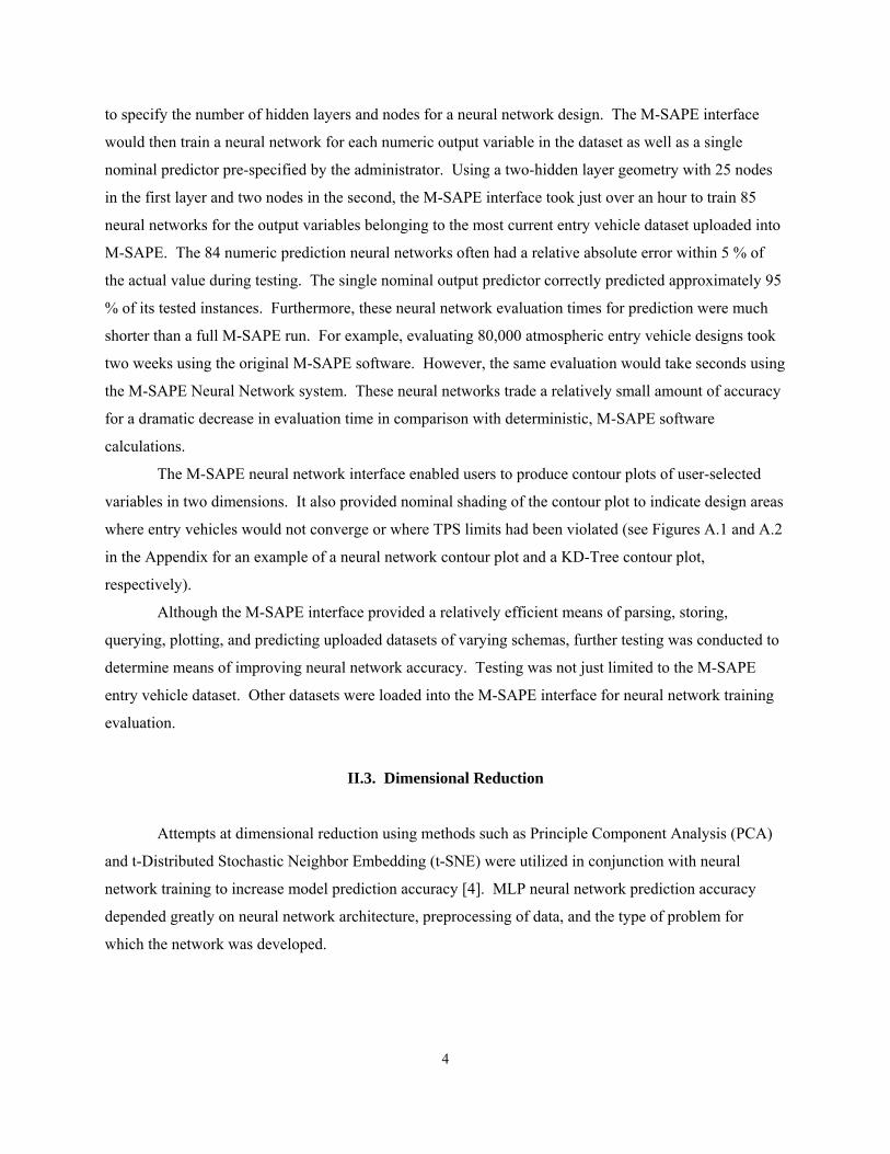
Figure 1. MLP Neural Network Generic Architecture
The input layer is made up of individual nodes, one node for each input parameter which will be
used to predict the output. The hidden layer(s) contain multilayer perceptron nodes which take input
values from the previous layer, calculate an output value, and then feed the output value forward to the
next layer. The output layer consists of a single node (for nominal predictions, it may contain multiple
nodes, one for each potential nominal output value) which receives input values from the previous hidden
layer and outputs the prediction for the model [2].
MLP neural networks must first be trained with representative data before they can be used to
make prediction. Neural networks evaluate training data and adjust node weights through a means called
backpropagation [2]. A Neural Network M-SAPE interface was developed which enabled administrators
4
to specify the number of hidden layers and nodes for a neural network design. The M-SAPE interface
would then train a neural network for each numeric output variable in the dataset as well as a single
nominal predictor pre-specified by the administrator. Using a two-hidden layer geometry with 25 nodes
in the first layer and two nodes in the second, the M-SAPE interface took just over an hour to train 85
neural networks for the output variables belonging to the most current entry vehicle dataset uploaded into
M-SAPE. The 84 numeric prediction neural networks often had a relative absolute error within 5 % of
the actual value during testing. The single nominal output predictor correctly predicted approximately 95
% of its tested instances. Furthermore, these neural network evaluation times for prediction were much
shorter than a full M-SAPE run. For example, evaluating 80,000 atmospheric entry vehicle designs took
two weeks using the original M-SAPE software. However, the same evaluation would take seconds using
the M-SAPE Neural Network system. These neural networks trade a relatively small amount of accuracy
for a dramatic decrease in evaluation time in comparison with deterministic, M-SAPE software
calculations.
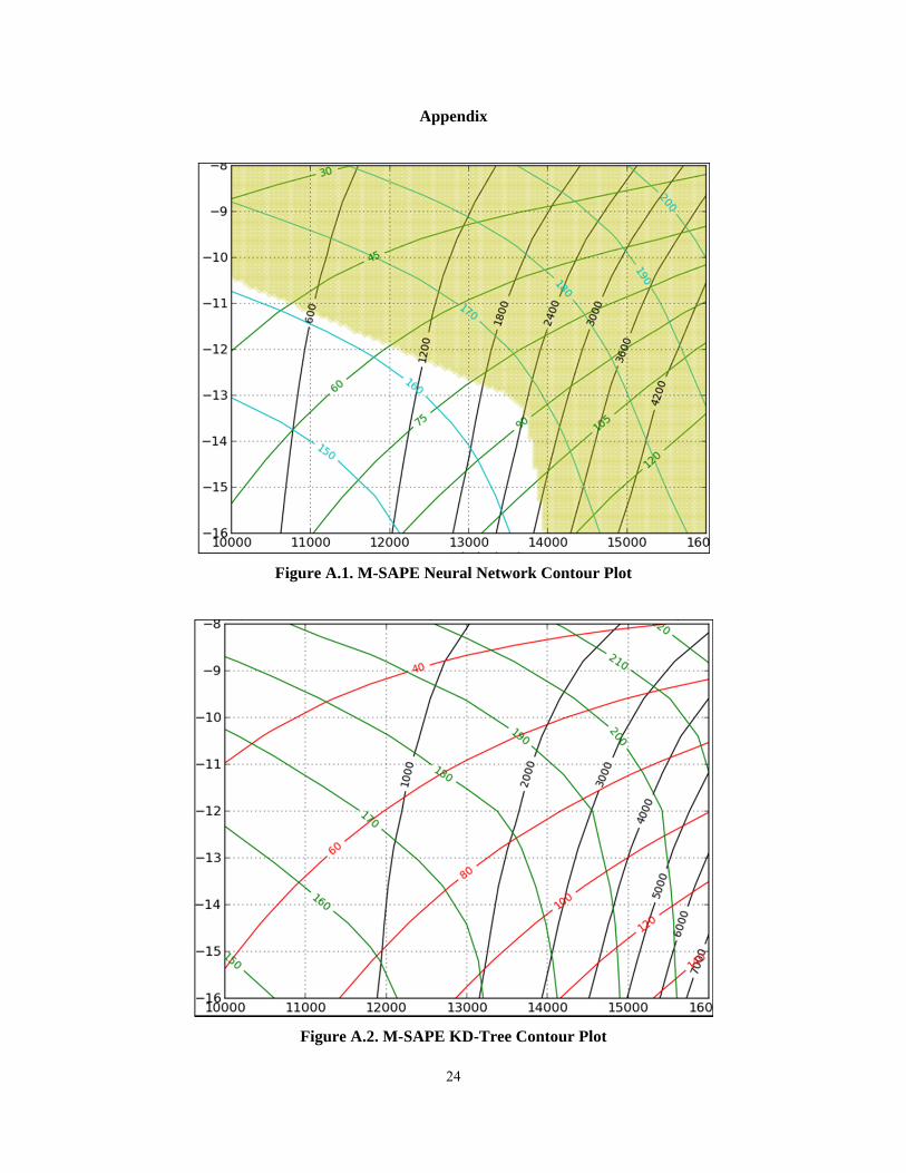
The M-SAPE neural network interface enabled users to produce contour plots of user-selected
variables in two dimensions. It also provided nominal shading of the contour plot to indicate design areas
where entry vehicles would not converge or where TPS limits had been violated (see Figures A.1 and A.2
in the Appendix for an example of a neural network contour plot and a KD-Tree contour plot,
respectively).
Although the M-SAPE interface provided a relatively efficient means of parsing, storing,
querying, plotting, and predicting uploaded datasets of varying schemas, further testing was conducted to
determine means of improving neural network accuracy. Testing was not just limited to the M-SAPE
entry vehicle dataset. Other datasets were loaded into the M-SAPE interface for neural network training
evaluation.
II.3. Dimensional Reduction
Attempts at dimensional reduction using methods such as Principle Component Analysis (PCA)
and t-Distributed Stochastic Neighbor Embedding (t-SNE) were utilized in conjunction with neural
network training to increase model prediction accuracy [4]. MLP neural network prediction accuracy
depended greatly on neural network architecture, preprocessing of data, and the type of problem for
which the network was developed.

5
III. Datasets
III.1. M-SAPE Entry Vehicle Dataset
As previously mentioned, M-SAPE datasets have 18 user-specified input variables. The M-SAPE
software will test the viability of user inputs and output over ninety nominal and numeric performance
characteristics.
The nominal outputs include vehicle convergence (whether or not the vehicle based on user input
parameters will be a viable design), TPS warnings (violations of the desired TPS model), etc. The
numeric outputs includes maximum total heat rate during entry, maximum entry load (measured in G-
forces), total entry mass, etc. M-SAPE entry vehicle datasets are nonlinear in nature.
III.2. Vehicle Side-Impact Crashworthiness Dataset
Vehicle side impact crashworthiness datasets were also generated using a Monte Carlo analysis
technique described in Ref. [5]. These crashworthiness datasets were created to analyze four-wheeled
vehicles (i.e., cars), not entry vehicles. Unlike the entry vehicle data, the crashworthiness datasets were
linear in nature [5].
The purpose of using the side-impact crashworthiness equations was to determine if neural
network approximation could match the accuracy of the Monte Carlo prediction using the equations.
III.3. LHS Datasets
LHS is a means of producing a smaller dataset that is still representative of all input variables
over either a normal or uniform distribution [6]. The goal of utilizing LHS was to minimize the number
of instances required to train a neural network. If a neural network could be trained to produce accurate
predictions using a smaller dataset, the time and computational requirements for training could be
dramatically reduced.
Datasets for entry vehicles and vehicle side-impact crashworthiness were generated using LHS.
6
III.4. MNIST Hand-Drawn Digit Grayscale Dataset
The MNIST dataset is a standard machine learning dataset provided by Ref. [8]. The dataset
consists of grayscale data for hand-drawn digits, and it contains 784 input variables which can be used to
predict what digit was drawn. The MNIST dataset was used to evaluate neural network training on an
extremely high-dimensional problem.
III.5. M-SAPE Data Upload Interface
The PHP M-SAPE interface was utilized to efficiently upload the heterogenous datasets into the
M-SAPE MySQL backend. Once data had been loaded into the system, neural network models could be
expediently trained and evaluated for prediction accuracy.
IV. Methods
IV.1. Neural Networks
Weka software was used for the training and evaluation of MLP neural networks. Training of
these networks was directly integrated into the M-SAPE PHP interface. Trained models could then be
stored on the M-SAPE server and utilized for predictions and contour plotting. The Weka software
utilized was capable of producing both nominal and numeric value predictions. Training with standard
entry vehicle datasets and with LHS-generated datasets was conducted.
IV.2. Data Pre-Processing and Dimensional Reduction
Techniques were also incorporated for pre-processing datasets prior to neural network training.
PCA and removal of non-essential variables were just two means of refining training datasets prior to
MLP network training with the goal of improving neural network accuracy.
Also, t-SNE was utilized for reducing multi-dimensional problems to just two dimensions for
plotting and data visualization [4]. Although an effective means for dimension reduction, t-SNE was
computationally cumbersome (running in O(n2) time). A more efficient version of t-SNE known as
Barnes-Hut t-Distributed Stochastic Neighbor Embedding (BH-SNE) was utilized in lieu of standard t-
7
SNE. This algorithm runs in O(n log n) time and is an effective means of quick dimension reduction with
little loss in fidelity compared with standard t-SNE [7].
Both t-SNE and BH-SNE are unsupervised methods of dimension reduction. Unlike a neural
network which compares a prediction with the actual value and then adjusts each node using
backpropagation, the SNE algorithms simply group input instances together in two dimensional space
based on the values of their input variables. The actual output value is never referenced during this
process of dimension reduction. However, the results can then be plotted in a two dimensional scatter
plot with a nominal color coding to show the actual output. If similar colors are clustered together, the
algorithm has effectively mapped a multi-dimensional problem into just two dimensions.
SNE techniques have often been used for unsupervised learning of gray scale images (such as the
MNIST dataset). For example, previous studies have shown t-SNE’s effectiveness at reducing over a
hundred dimensions representing grayscale, hand-written digits to just two dimensions. The results
revealed ten clusters representing each digit where like digits are clustered together [4].
During this set of tests, BH-SNE was used to not only map a nominal output for entry vehicle
performance, but to also map input variable values to separate scatter plots with the same plot pattern as
the output scatter plot. By comparing the output scatter plot with each input scatter plot, a user could
easily discover which input variable appears to have the highest effect on the output variable. A similar
colored scatter pattern between an output variable and a particular input variable would indicate a strong
relationship between the output and the input variable. This technique could be particularly useful in
multi-dimensional nonlinear problems where identifying which input variable has the highest effect on
the output is especially difficult.
V. Results
The ability of a neural network to provide accurate predictions depended greatly on the type of
problem being predicted, pre-processing techniques used prior to training, utilization of representative
sampling for network training, and the network architecture. Although PCA proved to be an effective
pre-processing technique for linear problems like vehicle side-impact crashworthiness, it actually
decreased prediction accuracy for nonlinear problems such as the M-SAPE entry vehicle dataset.
Improvements in nonlinear problem models could only be achieved by varying the architecture of the
neural network. While PCA was invaluable for identifying which input variables had the greatest impact
on the output for a linear problem, BH-SNE proved to be more effective for identifying relationships
between input and output in nonlinear problems. Using LHS proved to be an effective means of reducing
the required number of instances needed for MLP network training.
8
V.1. Neural Network Testing Results for Linear Problems
As mentioned above, multiple vehicle side impact crashworthiness datasets were used to build
neural networks. These datasets contained nine differing numeric input variables that determine 11
different numeric outputs. However, for each output variable, only a subset of the input variables were
actually used to calculate the output (using the Monte Carlo analysis presented in Ref. [5]). To determine
the accuracy of neural network prediction, all input variables were initially used to produce models for
each output variable. If the neural network backpropagation method was effective, then input variables
should be appropriately weighted according to their relationship to the output variable.
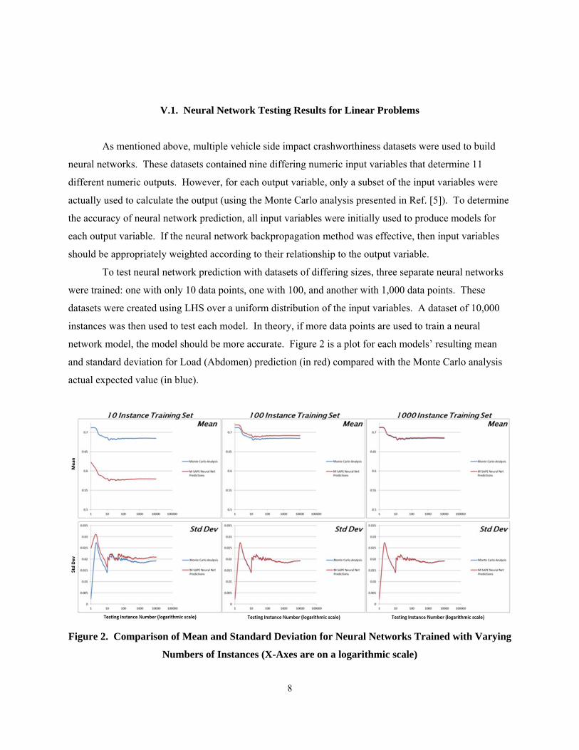
To test neural network prediction with datasets of differing sizes, three separate neural networks
were trained: one with only 10 data points, one with 100, and another with 1,000 data points. These
datasets were created using LHS over a uniform distribution of the input variables. A dataset of 10,000
instances was then used to test each model. In theory, if more data points are used to train a neural
network model, the model should be more accurate. Figure 2 is a plot for each models’ resulting mean
and standard deviation for Load (Abdomen) prediction (in red) compared with the Monte Carlo analysis
actual expected value (in blue).
Figure 2. Comparison of Mean and Standard Deviation for Neural Networks Trained with Varying
Numbers of Instances (X-Axes are on a logarithmic scale)
9
As the number of data points used to train each neural network increases, the mean and standard
deviation for its predictions more closely match those values produced by the Monte Carlo formulas used
to compute the actual values (shown in blue). However, it was possible to use LHS to reduce the number
of instances required for training (with a trade off in prediction accuracy).
As mentioned above, not all input variables were used to calculate certain outputs. For example,
the Load (Abdomen) function was as follows:
Load (Abdomen) = 1.16 – 0.3717 d2d4 – 0.00931 d2d10 – 0.484 d3d9 + 0.01343 d6d10
For this calculation, only the d2, d4, d10, d3, d9, and d6 variables were used to produce the actual
result using Monte Carlo Analysis. However, the neural networks trained for this example utilized every
variable for training of the models. If the backpropagation weighting method worked correctly during
training, then the neural network should have appropriately compensated for input variables which have
no impact on the actual output.
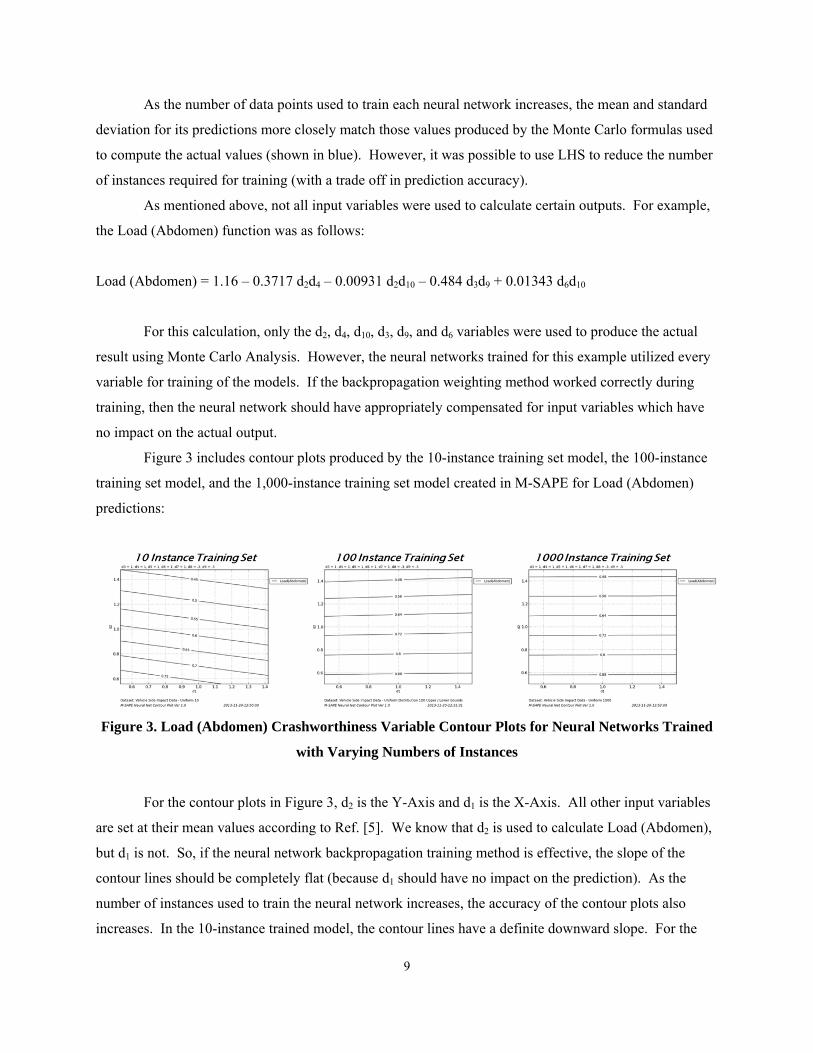
Figure 3 includes contour plots produced by the 10-instance training set model, the 100-instance
training set model, and the 1,000-instance training set model created in M-SAPE for Load (Abdomen)
predictions:
Figure 3. Load (Abdomen) Crashworthiness Variable Contour Plots for Neural Networks Trained
with Varying Numbers of Instances
For the contour plots in Figure 3, d2 is the Y-Axis and d1 is the X-Axis. All other input variables
are set at their mean values according to Ref. [5]. We know that d2 is used to calculate Load (Abdomen),
but d1 is not. So, if the neural network backpropagation training method is effective, the slope of the
contour lines should be completely flat (because d1 should have no impact on the prediction). As the
number of instances used to train the neural network increases, the accuracy of the contour plots also
increases. In the 10-instance trained model, the contour lines have a definite downward slope. For the
10
100-instance model, the lines have a very slight upward slope. The 1,000-instance trained model has an
even smaller upward slope than the 100-instance neural network. As expected, the neural network
backpropagation training technique is more effective when a larger dataset is used for training.
As mentioned above, PCA testing was also used in conjunction with neural net training. The
PCA technique pre-weights input variables based on their relationship to the output. Although PCA may
not completely eliminate an unnecessary input variable, it will give that variable an appropriately small
weight prior to feeding it to a neural network for training [2].
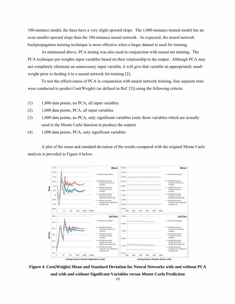
To test the effectiveness of PCA in conjunction with neural network training, four separate tests
were conducted to predict Cost(Weight) (as defined in Ref. [5]) using the following criteria:
(1) 1,000 data points, no PCA, all input variables
(2) 1,000 data points, PCA, all input variables
(3) 1,000 data points, no PCA, only significant variables (only those variables which are actually
used in the Monte Carlo function to produce the output)
(4) 1,000 data points, PCA, only significant variables
A plot of the mean and standard deviation of the results compared with the original Monte Carlo
analysis is provided in Figure 4 below.
Figure 4. Cost(Weight) Mean and Standard Deviation for Neural Networks with and without PCA
and with and without Significant Variables versus Monte Carlo Prediction
11
The horizontally adjacent plots in Figure 4 show the same data. The left graph uses the same
logarithmic X-axis as used in Figure 2 above, and the right graph shows an enlarged version of the mean
and standard deviation for the 9,995th testing data point upwards. On the left graph, the neural networks
trained using PCA with all variables, no PCA with only significant variables, and PCA with only
significant variables are plotted directly on top the Monte Carlo Analysis information (the enlarged graph
on the right is displayed to show the distinction between these four plots). The neural network with PCA
using all input variables most closely approximates the expected Monte Carlo actual value for mean
values. This value differs by less than 0.02% of the Monte Carlo analysis mean for the 9,999th instance
(reference the mean graph on the right above). The neural network without PCA trained only with
significant variables most closely approximates the standard deviation of the Monte Carlo analysis. This
neural network’s standard deviation prediction had only a difference of ~0.5% from the Monte Carlo
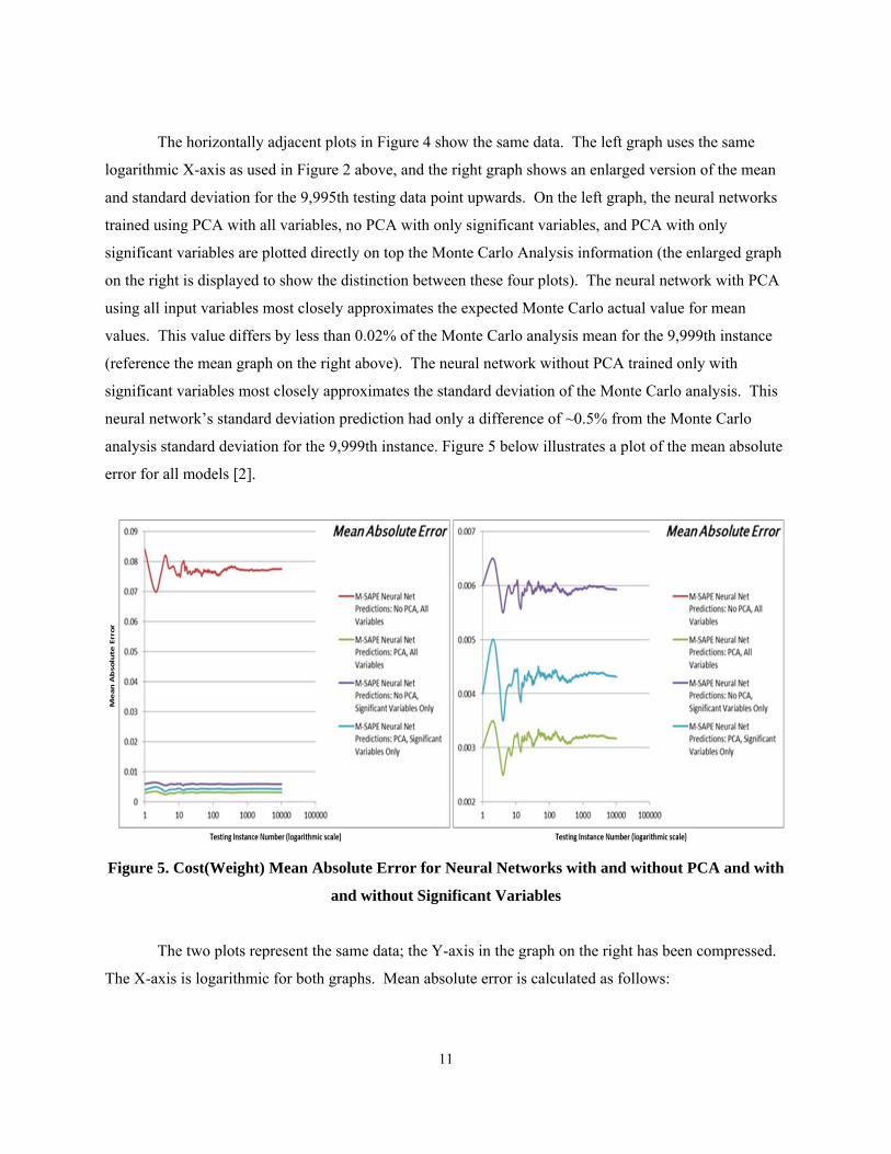
analysis standard deviation for the 9,999th instance. Figure 5 below illustrates a plot of the mean absolute
error for all models [2].
Figure 5. Cost(Weight) Mean Absolute Error for Neural Networks with and without PCA and with
and without Significant Variables
The two plots represent the same data; the Y-axis in the graph on the right has been compressed.
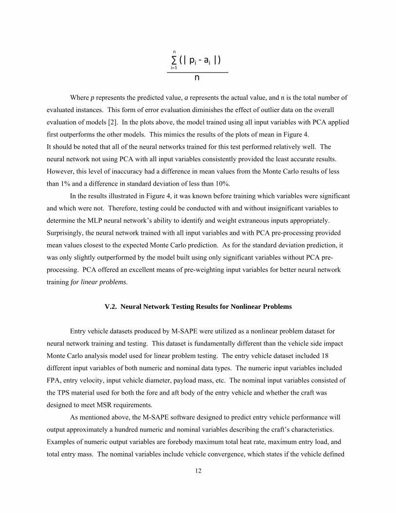
The X-axis is logarithmic for both graphs. Mean absolute error is calculated as follows:
12
Where p represents the predicted value, a represents the actual value, and n is the total number of
evaluated instances. This form of error evaluation diminishes the effect of outlier data on the overall
evaluation of models [2]. In the plots above, the model trained using all input variables with PCA applied
first outperforms the other models. This mimics the results of the plots of mean in Figure 4.
It should be noted that all of the neural networks trained for this test performed relatively well. The
neural network not using PCA with all input variables consistently provided the least accurate results.
However, this level of inaccuracy had a difference in mean values from the Monte Carlo results of less
than 1% and a difference in standard deviation of less than 10%.
In the results illustrated in Figure 4, it was known before training which variables were significant
and which were not. Therefore, testing could be conducted with and without insignificant variables to
determine the MLP neural network’s ability to identify and weight extraneous inputs appropriately.
Surprisingly, the neural network trained with all input variables and with PCA pre-processing provided
mean values closest to the expected Monte Carlo prediction. As for the standard deviation prediction, it
was only slightly outperformed by the model built using only significant variables without PCA pre-
processing. PCA offered an excellent means of pre-weighting input variables for better neural network
training for linear problems.
V.2. Neural Network Testing Results for Nonlinear Problems
Entry vehicle datasets produced by M-SAPE were utilized as a nonlinear problem dataset for
neural network training and testing. This dataset is fundamentally different than the vehicle side impact
Monte Carlo analysis model used for linear problem testing. The entry vehicle dataset included 18
different input variables of both numeric and nominal data types. The numeric input variables included
FPA, entry velocity, input vehicle diameter, payload mass, etc. The nominal input variables consisted of
the TPS material used for both the fore and aft body of the entry vehicle and whether the craft was
designed to meet MSR requirements.
As mentioned above, the M-SAPE software designed to predict entry vehicle performance will
output approximately a hundred numeric and nominal variables describing the craft’s characteristics.
Examples of numeric output variables are forebody maximum total heat rate, maximum entry load, and
total entry mass. The nominal variables include vehicle convergence, which states if the vehicle defined
13
per the user’s parameters will actually be a valid model. Other nominal output variables include forebody
and aftbody TPS warnings, which are textual descriptions of any potential TPS warnings for a vehicle on
entering the Earth’s atmosphere.
The deterministic M-SAPE vehicle prediction software iteratively adjusted a vehicle’s input
parameters if the initial specification did not produce a converged model. The process of evaluating a
single model took several minutes to complete. Due to the complexity of producing the output of a
vehicle’s performance, the M-SAPE entry vehicle dataset was excellent for the training and testing of
neural networks for nonlinear problems.
As noted above, PCA is a useful technique for pre-processing datasets prior to neural network
training for linear problems. To evaluate its effectiveness for a nonlinear problem, two separate MLP
networks were built to predict forebody maximum total heat rate. One model had PCA pre-processing
and the other did not. Both neural networks had a two-hidden layer architecture with 25 nodes in the first
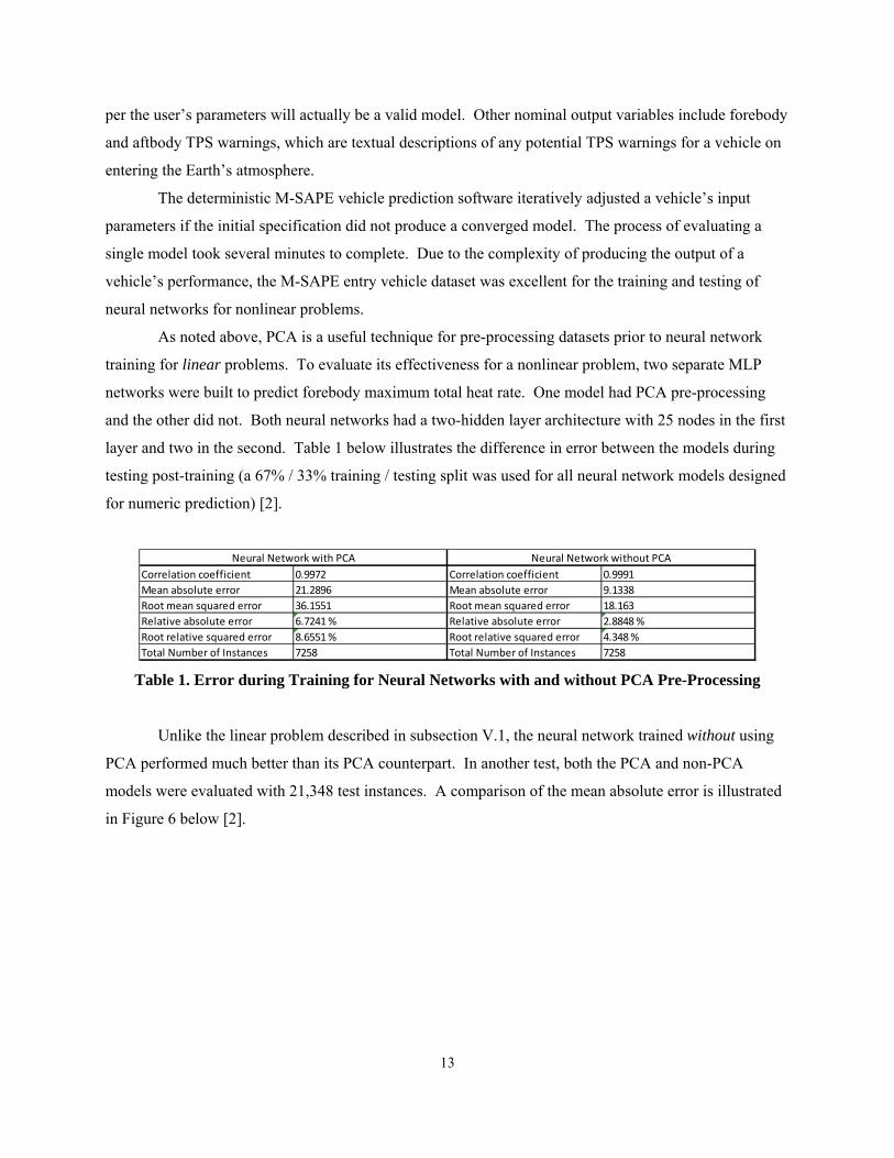
layer and two in the second. Table 1 below illustrates the difference in error between the models during
testing post-training (a 67% / 33% training / testing split was used for all neural network models designed
for numeric prediction) [2].
Table 1. Error during Training for Neural Networks with and without PCA Pre-Processing
Unlike the linear problem described in subsection V.1, the neural network trained without using
PCA performed much better than its PCA counterpart. In another test, both the PCA and non-PCA
models were evaluated with 21,348 test instances. A comparison of the mean absolute error is illustrated
in Figure 6 below [2].
Correlation coefficient 0.9972 Correlation coefficient 0.9991
Mean absolute error 21.2896 Mean absolute error 9.1338
Root mean squared error 36.1551 Root mean squared error 18.163
Relative absolute error 6.7241 % Relative absolute error 2.8848 %
Root relative squared error 8.6551 % Root relative squared error 4.348 %
Total Number of Instances 7258 Total Number of Instances 7258
Neural Network with PCA Neural Network without PCA
14
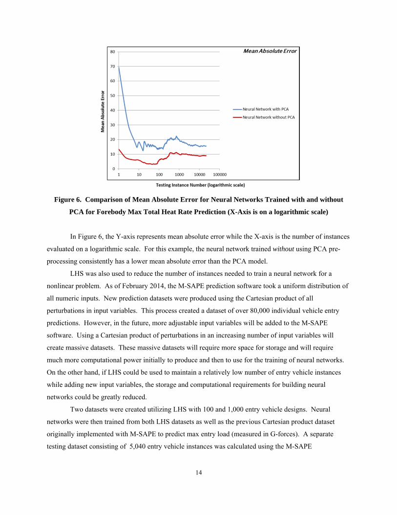
Figure 6. Comparison of Mean Absolute Error for Neural Networks Trained with and without
PCA for Forebody Max Total Heat Rate Prediction (X-Axis is on a logarithmic scale)
In Figure 6, the Y-axis represents mean absolute error while the X-axis is the number of instances
evaluated on a logarithmic scale. For this example, the neural network trained without using PCA pre-
processing consistently has a lower mean absolute error than the PCA model.
LHS was also used to reduce the number of instances needed to train a neural network for a
nonlinear problem. As of February 2014, the M-SAPE prediction software took a uniform distribution of
all numeric inputs. New prediction datasets were produced using the Cartesian product of all
perturbations in input variables. This process created a dataset of over 80,000 individual vehicle entry
predictions. However, in the future, more adjustable input variables will be added to the M-SAPE
software. Using a Cartesian product of perturbations in an increasing number of input variables will
create massive datasets. These massive datasets will require more space for storage and will require
much more computational power initially to produce and then to use for the training of neural networks.
On the other hand, if LHS could be used to maintain a relatively low number of entry vehicle instances
while adding new input variables, the storage and computational requirements for building neural
networks could be greatly reduced.
Two datasets were created utilizing LHS with 100 and 1,000 entry vehicle designs. Neural
networks were then trained from both LHS datasets as well as the previous Cartesian product dataset
originally implemented with M-SAPE to predict max entry load (measured in G-forces). A separate
testing dataset consisting of 5,040 entry vehicle instances was calculated using the M-SAPE
15
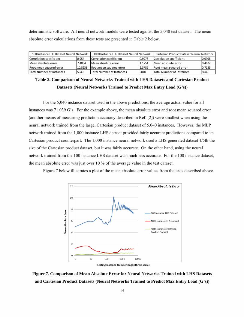
deterministic software. All neural network models were tested against the 5,040 test dataset. The mean
absolute error calculations from these tests are presented in Table 2 below.
Table 2. Comparison of Neural Networks Trained with LHS Datasets and Cartesian Product
Datasets (Neural Networks Trained to Predict Max Entry Load (G’s))
For the 5,040 instance dataset used in the above predictions, the average actual value for all
instances was 71.039 G’s. For the example above, the mean absolute error and root mean squared error
(another means of measuring prediction accuracy described in Ref. [2]) were smallest when using the
neural network trained from the large, Cartesian product dataset of 5,040 instances. However, the MLP
network trained from the 1,000 instance LHS dataset provided fairly accurate predictions compared to its
Cartesian product counterpart. The 1,000 instance neural network used a LHS generated dataset 1/5th the
size of the Cartesian product dataset, but it was fairly accurate. On the other hand, using the neural
network trained from the 100 instance LHS dataset was much less accurate. For the 100 instance dataset,
the mean absolute error was just over 10 % of the average value in the test dataset.
Figure 7 below illustrates a plot of the mean absolute error values from the tests described above.
Figure 7. Comparison of Mean Absolute Error for Neural Networks Trained with LHS Datasets
and Cartesian Product Datasets (Neural Networks Trained to Predict Max Entry Load (G’s))
Correlation coefficient 0.954 Correlation coefficient 0.9978 Correlation coefficient 0.9998
Mean absolute error 7.4034 Mean absolute error 1.1751 Mean absolute error 0.4622
Root mean squared error 10.8238 Root mean squared error 2.3786 Root mean squared error 0.7135
Total Number of Instances 5040 Total Number of Instances 5040 Total Number of Instances 5040
100 Instance LHS Dataset Neural Network 1000 Instance LHS Dataset Neural Network Cartesian Product Dataset Neural Network
16
Although the neural network trained with 5,040 instances provided the most accurate results, the
1,000 instance LHS dataset provided a fairly small loss of accuracy while using much less data to train
the MLP network model. The network trained with the100 instance LHS dataset, on the other hand,
produced a much higher deviation in mean absolute error than the other two networks.
V.3. Neural Network Testing Results for Nonlinear, High Dimensional Problems
Testing on nonlinear datasets of high dimensionality were also conducted using the MNIST
dataset. This dataset had 784 input variables used to predict a hand-written digit [8]. Using a neural
network consisting of two layers with 25 nodes in the first layer and two nodes in the second, a neural
network model with an accuracy of 76.4706 % was created. Another two layer model with 50 nodes in
the first layer and four nodes in the second layer accurately predicted the drawn digit for 79.5294 % of the
test instances. Yet another two layer model with 100 nodes in the first layer and eight nodes in the second
layer provided a prediction accuracy of 87.1765 %. Varying the network geometry by increasing the
number of nodes in each layer increased the accuracy of models built for extremely high dimensional
problems.
V.4. Nonlinear Dimension Reduction and Visualization
Although PCA failed to produce more accurate prediction models for nonlinear problems, BH-
SNE was also utilized to reduce multidimensional problems to just two dimensions for neural network
training as well as for plotting. As mentioned above, BH-SNE is an unsupervised method of reducing
dimensionality. BH-SNE is also specifically implemented for nominal value predictions. [7]
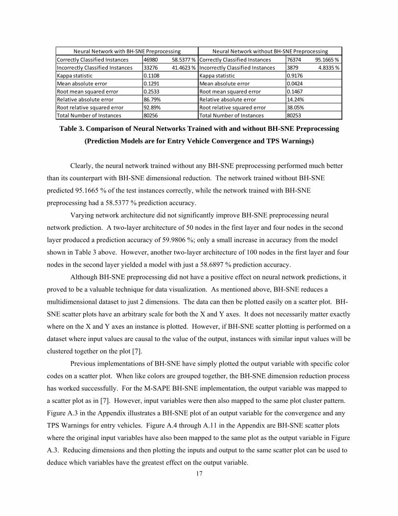
To evaluate the effectiveness of BH-SNE dimension reductions, a dataset for predicting entry
vehicle convergence and TPS warning messages was produced using BH-SNE dimensional reduction to
create just two input variables. Two nominal neural network prediction models were then created, one
using the BH-SNE dataset and the other using all original input variables. A two--layer architectures of
25 nodes in the first layer and two nodes in the second were implemented for both models. Table 3 below
shows a comparison of the results for training both models.
17
Table 3. Comparison of Neural Networks Trained with and without BH-SNE Preprocessing
(Prediction Models are for Entry Vehicle Convergence and TPS Warnings)
Clearly, the neural network trained without any BH-SNE preprocessing performed much better
than its counterpart with BH-SNE dimensional reduction. The network trained without BH-SNE
predicted 95.1665 % of the test instances correctly, while the network trained with BH-SNE
preprocessing had a 58.5377 % prediction accuracy.
Varying network architecture did not significantly improve BH-SNE preprocessing neural
network prediction. A two-layer architecture of 50 nodes in the first layer and four nodes in the second
layer produced a prediction accuracy of 59.9806 %; only a small increase in accuracy from the model
shown in Table 3 above. However, another two-layer architecture of 100 nodes in the first layer and four
nodes in the second layer yielded a model with just a 58.6897 % prediction accuracy.
Although BH-SNE preprocessing did not have a positive effect on neural network predictions, it
proved to be a valuable technique for data visualization. As mentioned above, BH-SNE reduces a
multidimensional dataset to just 2 dimensions. The data can then be plotted easily on a scatter plot. BH-
SNE scatter plots have an arbitrary scale for both the X and Y axes. It does not necessarily matter exactly
where on the X and Y axes an instance is plotted. However, if BH-SNE scatter plotting is performed on a
dataset where input values are causal to the value of the output, instances with similar input values will be
clustered together on the plot [7].
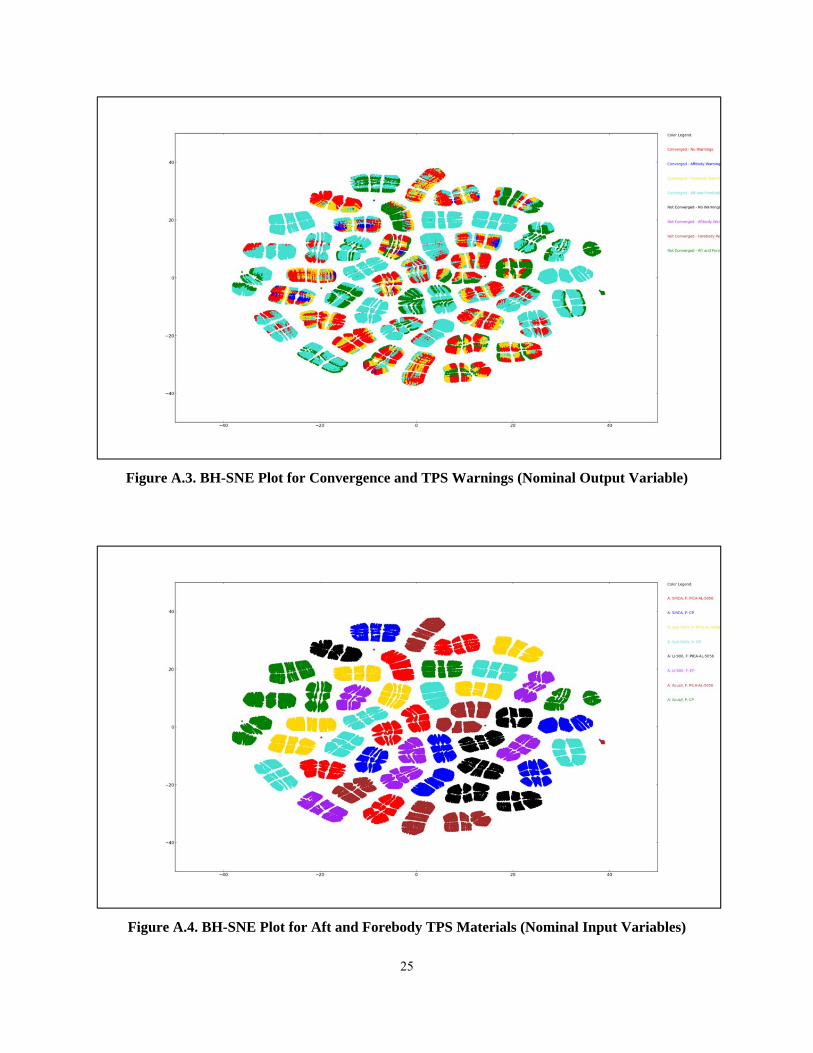
Previous implementations of BH-SNE have simply plotted the output variable with specific color
codes on a scatter plot. When like colors are grouped together, the BH-SNE dimension reduction process
has worked successfully. For the M-SAPE BH-SNE implementation, the output variable was mapped to
a scatter plot as in [7]. However, input variables were then also mapped to the same plot cluster pattern.
Figure A.3 in the Appendix illustrates a BH-SNE plot of an output variable for the convergence and any
TPS Warnings for entry vehicles. Figure A.4 through A.11 in the Appendix are BH-SNE scatter plots
where the original input variables have also been mapped to the same plot as the output variable in Figure
A.3. Reducing dimensions and then plotting the inputs and output to the same scatter plot can be used to
deduce which variables have the greatest effect on the output variable.
Correctly Classified Instances 46980 58.5377 % Correctly Classified Instances 76374 95.1665 %
Incorrectly Classified Instances 33276 41.4623 % Incorrectly Classified Instances 3879 4.8335 %
Kappa statistic 0.1108 Kappa statistic 0.9176
Mean absolute error 0.1291 Mean absolute error 0.0424
Root mean squared error 0.2533 Root mean squared error 0.1467
Relative absolute error 86.79% Relative absolute error 14.24%
Root relative squared error 92.89% Root relative squared error 38.05%
Total Number of Instances 80256 Total Number of Instances 80253
Neural Network with BH‐SNE Preprocessing Neural Network without BH‐SNE Preprocessing
18
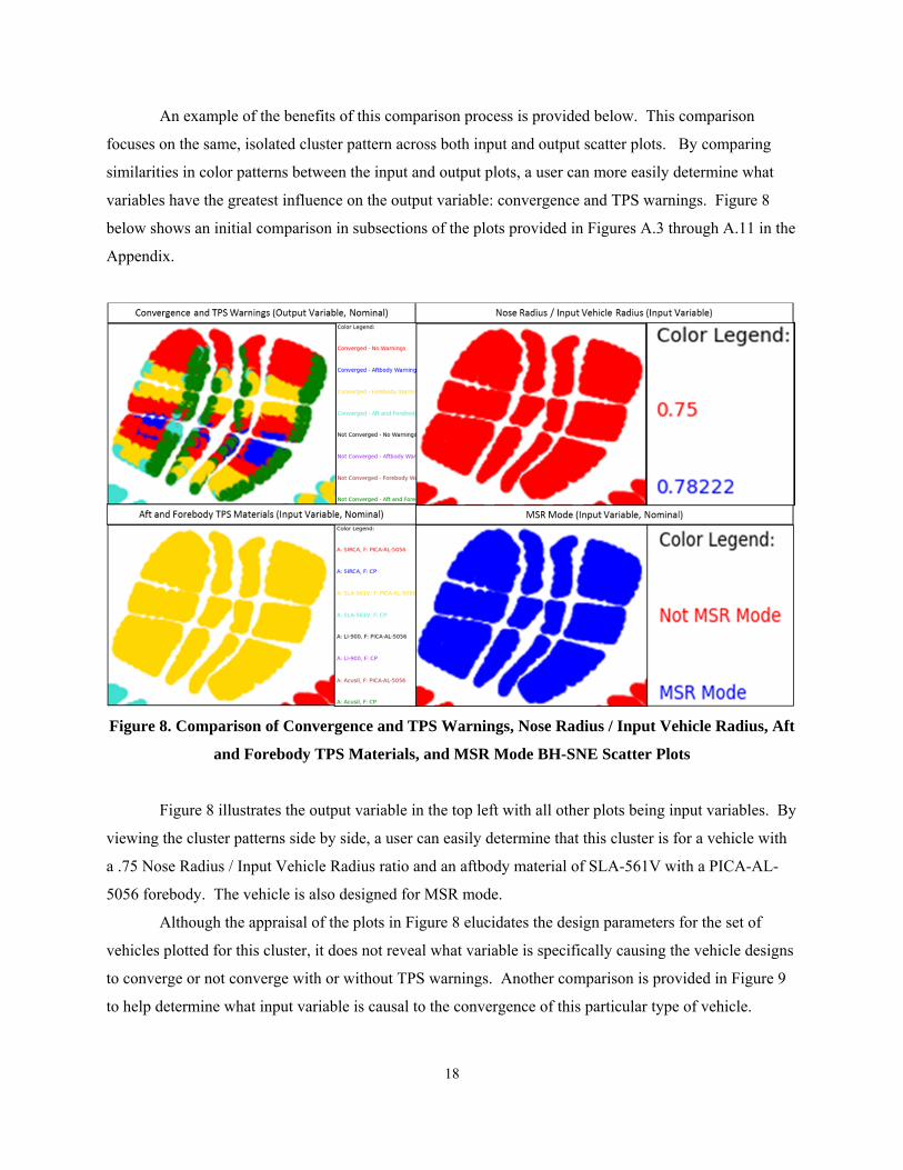
An example of the benefits of this comparison process is provided below. This comparison
focuses on the same, isolated cluster pattern across both input and output scatter plots. By comparing
similarities in color patterns between the input and output plots, a user can more easily determine what
variables have the greatest influence on the output variable: convergence and TPS warnings. Figure 8
below shows an initial comparison in subsections of the plots provided in Figures A.3 through A.11 in the
Appendix.
Figure 8. Comparison of Convergence and TPS Warnings, Nose Radius / Input Vehicle Radius, Aft
and Forebody TPS Materials, and MSR Mode BH-SNE Scatter Plots
Figure 8 illustrates the output variable in the top left with all other plots being input variables. By
viewing the cluster patterns side by side, a user can easily determine that this cluster is for a vehicle with
a .75 Nose Radius / Input Vehicle Radius ratio and an aftbody material of SLA-561V with a PICA-AL-
5056 forebody. The vehicle is also designed for MSR mode.
Although the appraisal of the plots in Figure 8 elucidates the design parameters for the set of
vehicles plotted for this cluster, it does not reveal what variable is specifically causing the vehicle designs
to converge or not converge with or without TPS warnings. Another comparison is provided in Figure 9
to help determine what input variable is causal to the convergence of this particular type of vehicle.
19
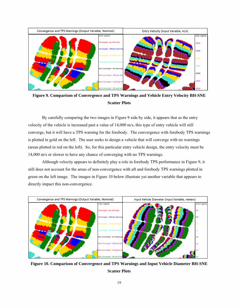
Figure 9. Comparison of Convergence and TPS Warnings and Vehicle Entry Velocity BH-SNE
Scatter Plots
By carefully comparing the two images in Figure 9 side by side, it appears that as the entry
velocity of the vehicle is increased past a value of 14,000 m/s, this type of entry vehicle will still
converge, but it will have a TPS warning for the forebody. The convergence with forebody TPS warnings
is plotted in gold on the left. The user seeks to design a vehicle that will converge with no warnings
(areas plotted in red on the left). So, for this particular entry vehicle design, the entry velocity must be
14,000 m/s or slower to have any chance of converging with no TPS warnings.
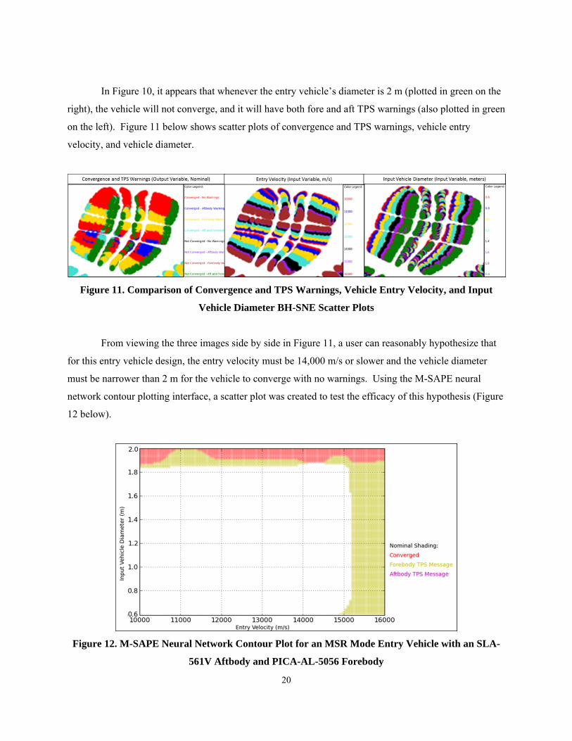
Although velocity appears to definitely play a role in forebody TPS performance in Figure 9, it
still does not account for the areas of non-convergence with aft and forebody TPS warnings plotted in
green on the left image. The images in Figure 10 below illustrate yet another variable that appears to
directly impact this non-convergence.
Figure 10. Comparison of Convergence and TPS Warnings and Input Vehicle Diameter BH-SNE
Scatter Plots
20
In Figure 10, it appears that whenever the entry vehicle’s diameter is 2 m (plotted in green on the
right), the vehicle will not converge, and it will have both fore and aft TPS warnings (also plotted in green
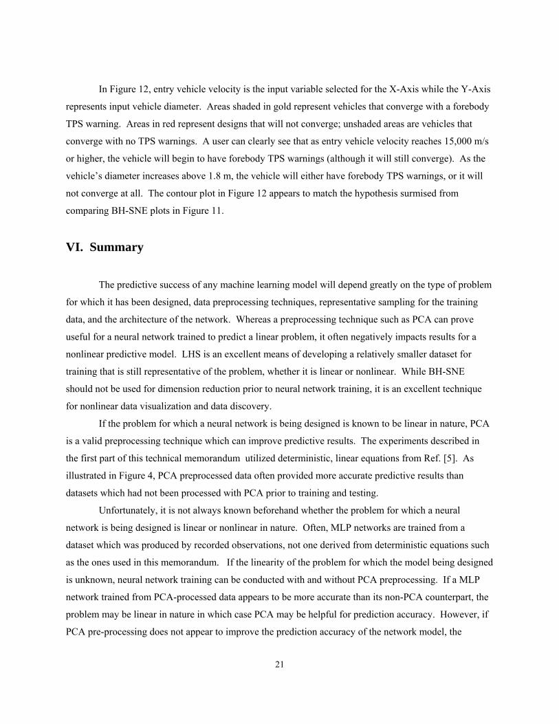
on the left). Figure 11 below shows scatter plots of convergence and TPS warnings, vehicle entry
velocity, and vehicle diameter.
Figure 11. Comparison of Convergence and TPS Warnings, Vehicle Entry Velocity, and Input
Vehicle Diameter BH-SNE Scatter Plots
From viewing the three images side by side in Figure 11, a user can reasonably hypothesize that
for this entry vehicle design, the entry velocity must be 14,000 m/s or slower and the vehicle diameter
must be narrower than 2 m for the vehicle to converge with no warnings. Using the M-SAPE neural
network contour plotting interface, a scatter plot was created to test the efficacy of this hypothesis (Figure
12 below).
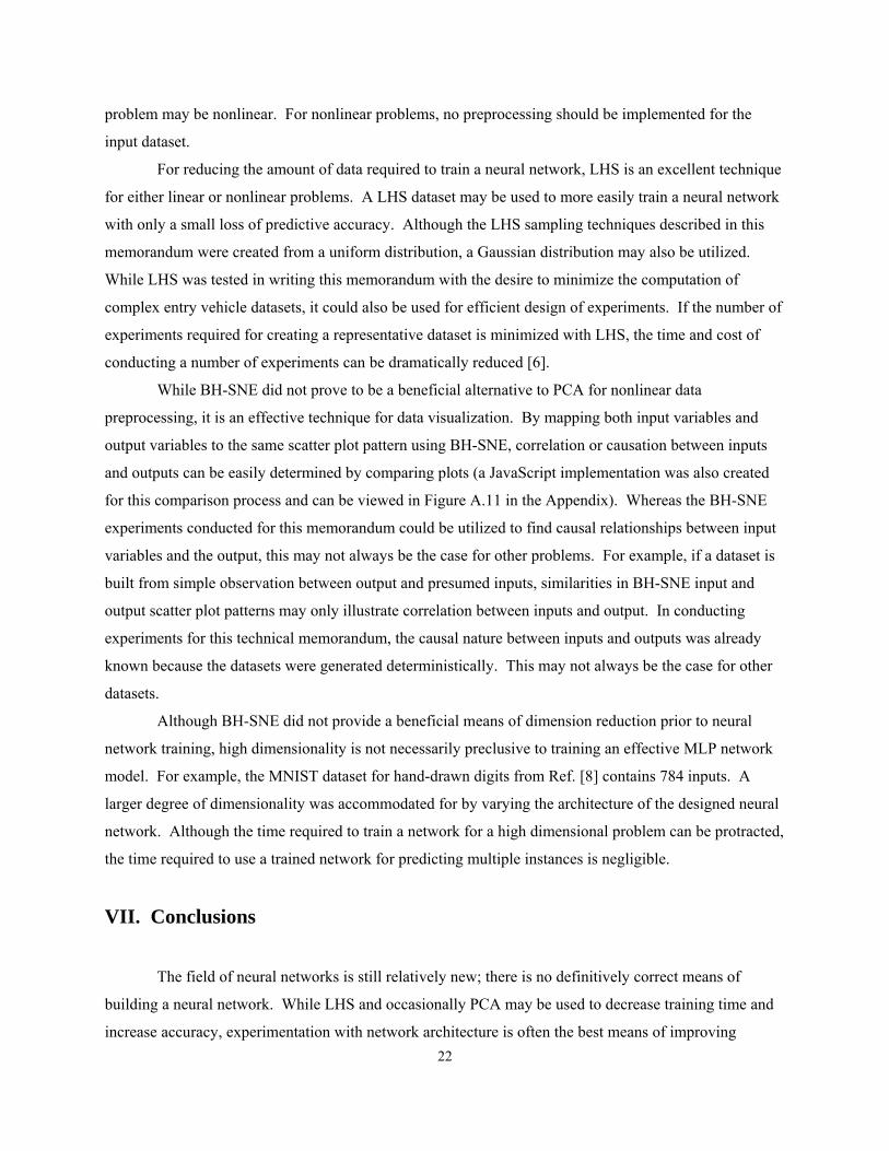
Figure 12. M-SAPE Neural Network Contour Plot for an MSR Mode Entry Vehicle with an SLA-
561V Aftbody and PICA-AL-5056 Forebody
21
In Figure 12, entry vehicle velocity is the input variable selected for the X-Axis while the Y-Axis
represents input vehicle diameter. Areas shaded in gold represent vehicles that converge with a forebody
TPS warning. Areas in red represent designs that will not converge; unshaded areas are vehicles that
converge with no TPS warnings. A user can clearly see that as entry vehicle velocity reaches 15,000 m/s
or higher, the vehicle will begin to have forebody TPS warnings (although it will still converge). As the
vehicle’s diameter increases above 1.8 m, the vehicle will either have forebody TPS warnings, or it will
not converge at all. The contour plot in Figure 12 appears to match the hypothesis surmised from
comparing BH-SNE plots in Figure 11.
VI. Summary
The predictive success of any machine learning model will depend greatly on the type of problem
for which it has been designed, data preprocessing techniques, representative sampling for the training
data, and the architecture of the network. Whereas a preprocessing technique such as PCA can prove
useful for a neural network trained to predict a linear problem, it often negatively impacts results for a
nonlinear predictive model. LHS is an excellent means of developing a relatively smaller dataset for
training that is still representative of the problem, whether it is linear or nonlinear. While BH-SNE
should not be used for dimension reduction prior to neural network training, it is an excellent technique
for nonlinear data visualization and data discovery.
If the problem for which a neural network is being designed is known to be linear in nature, PCA
is a valid preprocessing technique which can improve predictive results. The experiments described in
the first part of this technical memorandum utilized deterministic, linear equations from Ref. [5]. As
illustrated in Figure 4, PCA preprocessed data often provided more accurate predictive results than
datasets which had not been processed with PCA prior to training and testing.
Unfortunately, it is not always known beforehand whether the problem for which a neural
network is being designed is linear or nonlinear in nature. Often, MLP networks are trained from a
dataset which was produced by recorded observations, not one derived from deterministic equations such
as the ones used in this memorandum. If the linearity of the problem for which the model being designed
is unknown, neural network training can be conducted with and without PCA preprocessing. If a MLP
network trained from PCA-processed data appears to be more accurate than its non-PCA counterpart, the
problem may be linear in nature in which case PCA may be helpful for prediction accuracy. However, if
PCA pre-processing does not appear to improve the prediction accuracy of the network model, the
22
problem may be nonlinear. For nonlinear problems, no preprocessing should be implemented for the
input dataset.
For reducing the amount of data required to train a neural network, LHS is an excellent technique
for either linear or nonlinear problems. A LHS dataset may be used to more easily train a neural network
with only a small loss of predictive accuracy. Although the LHS sampling techniques described in this
memorandum were created from a uniform distribution, a Gaussian distribution may also be utilized.
While LHS was tested in writing this memorandum with the desire to minimize the computation of
complex entry vehicle datasets, it could also be used for efficient design of experiments. If the number of
experiments required for creating a representative dataset is minimized with LHS, the time and cost of
conducting a number of experiments can be dramatically reduced [6].
While BH-SNE did not prove to be a beneficial alternative to PCA for nonlinear data
preprocessing, it is an effective technique for data visualization. By mapping both input variables and
output variables to the same scatter plot pattern using BH-SNE, correlation or causation between inputs
and outputs can be easily determined by comparing plots (a JavaScript implementation was also created
for this comparison process and can be viewed in Figure A.11 in the Appendix). Whereas the BH-SNE
experiments conducted for this memorandum could be utilized to find causal relationships between input
variables and the output, this may not always be the case for other problems. For example, if a dataset is
built from simple observation between output and presumed inputs, similarities in BH-SNE input and
output scatter plot patterns may only illustrate correlation between inputs and output. In conducting
experiments for this technical memorandum, the causal nature between inputs and outputs was already
known because the datasets were generated deterministically. This may not always be the case for other
datasets.
Although BH-SNE did not provide a beneficial means of dimension reduction prior to neural
network training, high dimensionality is not necessarily preclusive to training an effective MLP network
model. For example, the MNIST dataset for hand-drawn digits from Ref. [8] contains 784 inputs. A
larger degree of dimensionality was accommodated for by varying the architecture of the designed neural
network. Although the time required to train a network for a high dimensional problem can be protracted,
the time required to use a trained network for predicting multiple instances is negligible.
VII. Conclusions
The field of neural networks is still relatively new; there is no definitively correct means of
building a neural network. While LHS and occasionally PCA may be used to decrease training time and
increase accuracy, experimentation with network architecture is often the best means of improving

23
predictive results. The BH-SNE data visualization technique, used in conjunction with neural network
testing, is also an excellent means of machine learning data discovery. Experimentation with the different
techniques described in this memorandum can help improve neural network training and can illuminate
causal relationships between neural network input and output variables.
24
Appendix
Figure A.1. M-SAPE Neural Network Contour Plot
Figure A.2. M-SAPE KD-Tree Contour Plot
25
Figure A.3. BH-SNE Plot for Convergence and TPS Warnings (Nominal Output Variable)
Figure A.4. BH-SNE Plot for Aft and Forebody TPS Materials (Nominal Input Variables)
26
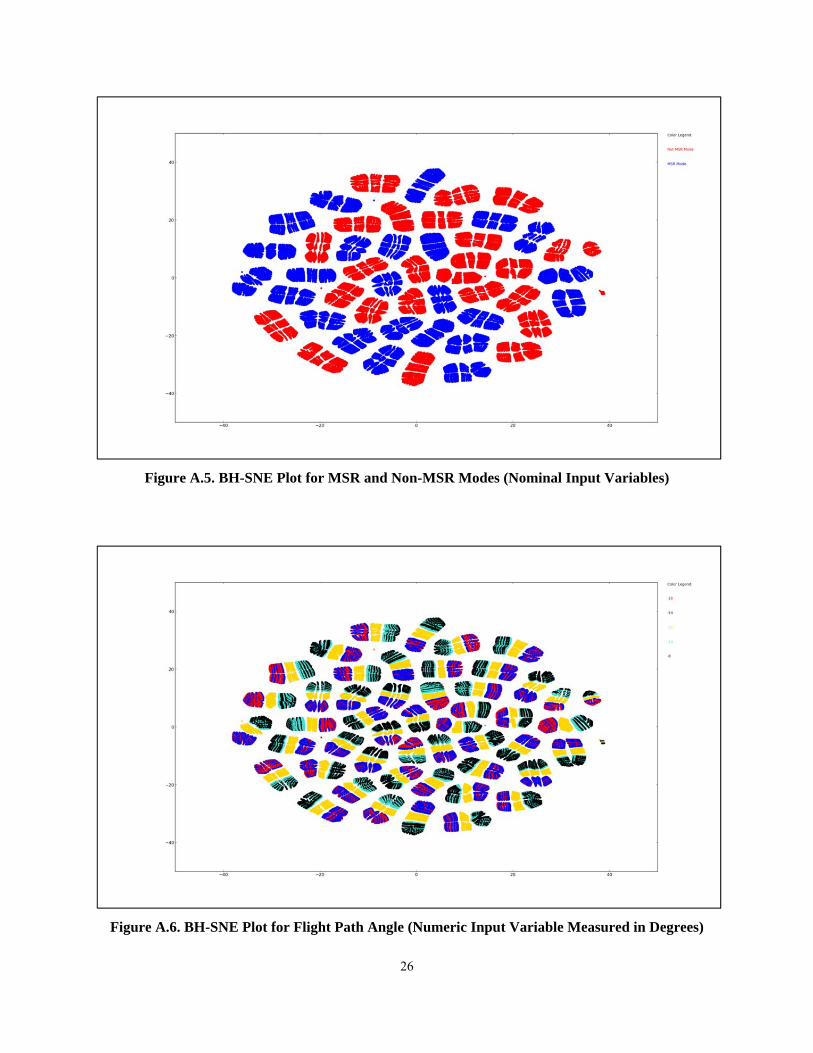
Figure A.5. BH-SNE Plot for MSR and Non-MSR Modes (Nominal Input Variables)
Figure A.6. BH-SNE Plot for Flight Path Angle (Numeric Input Variable Measured in Degrees)
27
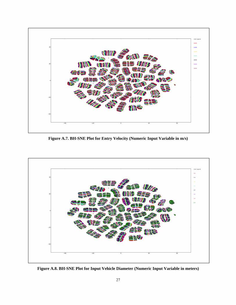
Figure A.7. BH-SNE Plot for Entry Velocity (Numeric Input Variable in m/s)
Figure A.8. BH-SNE Plot for Input Vehicle Diameter (Numeric Input Variable in meters)
28
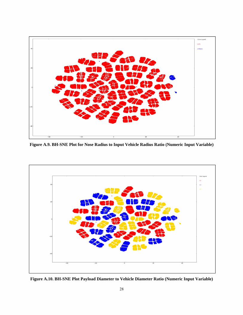
Figure A.9. BH-SNE Plot for Nose Radius to Input Vehicle Radius Ratio (Numeric Input Variable)
Figure A.10. BH-SNE Plot Payload Diameter to Vehicle Diameter Ratio (Numeric Input Variable)
29
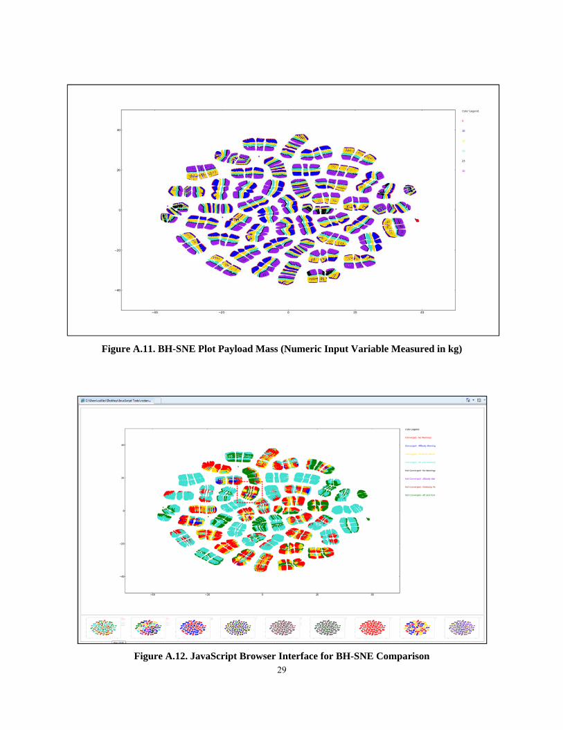
Figure A.11. BH-SNE Plot Payload Mass (Numeric Input Variable Measured in kg)
Figure A.12. JavaScript Browser Interface for BH-SNE Comparison

30
References
1. L. Wang. (2014). High Dimensional Data Analysis [Online]. Available:
http://lilywang.myweb.uga.edu/Research/highdimension.pdf
2. I.H. Witten et al., Data Mining: Practical Machine Learning Tools and Techniques (3rd ed.).
Burlington, MA: Elsevier Inc., 2011.
3. J.A. Samareh et al. (2012). An Integrated Tool for System Analysis of Sample Return Vehicles
[Online]. Available:
http://ntrs.nasa.gov/archive/nasa/casi.ntrs.nasa.gov/20120003332_2012003559.pdf
4. L.V.D. Maaten and G. Hinton. (2008). Visualizing Data using t-SNE [Online]. Available:
http://siplab.tudelft.nl/sites/default/files/vandermaaten08a.pdf
5. B.D. Youn et al. (2004). Reliability-based design optimization for crashworthiness of vehicle side
impact [Online]. Available:
http://download.springer.com/static/pdf/149/art%253A10.1007%252Fs00158-003-0345-
0.pdf?auth66=1392996180_98737b36e4e9eb28a9cca086a8c973d0&ext=.pdf
6. A. Olsson et al. (2003). On Latin hypercube sampling for structural reliability analysis [Online].
Available: http://www.sciencedirect.com/science/article/pii/S0167473002000395
7. L.V.D. Maaten. (2013). Barnes-Hut-SNE [Online]. Available: http://arxiv.org/pdf/1301.3342v2.pdf
8. LeCun, Y. et al. (1998). The MNIST Database of Handwritten Digits [Online]. Available:
http://yann.lecun.com/exdb/mnist/

REPORT DOCUMENTATION PAGEForm Approved
OMB No. 0704-0188
2. REPORT TYPE
Technical Memorandum 4. TITLE AND SUBTITLE
Neural Network Machine Learning and Dimension Reduction for Data Visualization
5a. CONTRACT NUMBER
6. AUTHOR(S)
Liles, Charles A.
7. PERFORMING ORGANIZATION NAME(S) AND ADDRESS(ES)
NASA Langley Research CenterHampton, VA 23681-2199
9. SPONSORING/MONITORING AGENCY NAME(S) AND ADDRESS(ES)
National Aeronautics and Space AdministrationWashington, DC 20546-0001
8. PERFORMING ORGANIZATION REPORT NUMBER
L-20389
10. SPONSOR/MONITOR'S ACRONYM(S)
NASA
13. SUPPLEMENTARY NOTES
This work was performed by Charles Liles under the Langley Aerospace Research Summer Scholar (LARSS) program.
12. DISTRIBUTION/AVAILABILITY STATEMENTUnclassified - UnlimitedSubject Category 59Availability: NASA CASI (443) 757-5802
19a. NAME OF RESPONSIBLE PERSON
STI Help Desk (email: [email protected])
14. ABSTRACT
Neural network machine learning in computer science is a continuously developing field of study. Although neural network models have been developed which can accurately predict a numeric value or nominal classification, a general purpose method for constructing neural network architecture has yet to be developed. Computer scientists are often forced to rely on a trial-and-error process of developing and improving accurate neural network models. In many cases, models are constructed from a large number of input parameters. Understanding which input parameters have the greatest impact on the prediction of the model is often difficult to surmise, especially when the number of input variables is very high.This challenge is often labeled the “curse of dimensionality” in scientific fields. However, techniques exist for reducing the dimensionality of problems to just two dimensions. Once a problem’s dimensions have been mapped to two dimensions, it can be easily plotted and understood by humans. The ability to visualize a multi-dimensional dataset can provide a means of identifying which input variables have the highest effect on determining a nominal or numeric output. Identifying these variables can provide a better means of training neural network models; models can be more easily and quickly trained using only input variables which appear to affect the outcome variable. The purpose of this project is to explore varying means of training neural networks and to utilize dimensional reduction for visualizing and understanding complex datasets.
15. SUBJECT TERMS
Dimension reduction; Machine learning; Neural network; Systems analysis
18. NUMBER OF PAGES
3519b. TELEPHONE NUMBER (Include area code)
(443) 757-5802
a. REPORT
U
c. THIS PAGE
U
b. ABSTRACT
U
17. LIMITATION OF ABSTRACT
UU
Prescribed by ANSI Std. Z39.18Standard Form 298 (Rev. 8-98)
3. DATES COVERED (From - To)
5b. GRANT NUMBER
5c. PROGRAM ELEMENT NUMBER
5d. PROJECT NUMBER
5e. TASK NUMBER
5f. WORK UNIT NUMBER
346620.04.07.01.01.02
11. SPONSOR/MONITOR'S REPORT NUMBER(S)
NASA/TM-2014-218181
16. SECURITY CLASSIFICATION OF:
The public reporting burden for this collection of information is estimated to average 1 hour per response, including the time for reviewing instructions, searching existing data sources, gathering and maintaining the data needed, and completing and reviewing the collection of information. Send comments regarding this burden estimate or any other aspect of this collection of information, including suggestions for reducing this burden, to Department of Defense, Washington Headquarters Services, Directorate for Information Operations and Reports (0704-0188), 1215 Jefferson Davis Highway, Suite 1204, Arlington, VA 22202-4302. Respondents should be aware that notwithstanding any other provision of law, no person shall be subject to any penalty for failing to comply with a collection of information if it does not display a currently valid OMB control number.PLEASE DO NOT RETURN YOUR FORM TO THE ABOVE ADDRESS.
1. REPORT DATE (DD-MM-YYYY)
03 - 201401-