August 2011

NASA/TM–2011-217169

Development of the Transport Class Model (TCM) Aircraft Simulation From a Sub-Scale Generic Transport Model (GTM) Simulation Richard M. Hueschen Langley Research Center, Hampton, Virginia

https://ntrs.nasa.gov/search.jsp?R=20110014509 2018-07-09T03:50:31+00:00Z

NASA STI Program . . . in Profile

Since its founding, NASA has been dedicated to the advancement of aeronautics and space science. The NASA scientific and technical information (STI) program plays a key part in helping NASA maintain this important role.

The NASA STI program operates under the auspices of the Agency Chief Information Officer. It collects, organizes, provides for archiving, and disseminates NASA’s STI. The NASA STI program provides access to the NASA Aeronautics and Space Database and its public interface, the NASA Technical Report Server, thus providing one of the largest collections of aeronautical and space science STI in the world. Results are published in both non-NASA channels and by NASA in the NASA STI Report Series, which includes the following report types:

TECHNICAL PUBLICATION. Reports of

completed research or a major significant phase of research that present the results of NASA programs and include extensive data or theoretical analysis. Includes compilations of significant scientific and technical data and information deemed to be of continuing reference value. NASA counterpart of peer-reviewed formal professional papers, but having less stringent limitations on manuscript length and extent of graphic presentations.

TECHNICAL MEMORANDUM. Scientific

and technical findings that are preliminary or of specialized interest, e.g., quick release reports, working papers, and bibliographies that contain minimal annotation. Does not contain extensive analysis.

CONTRACTOR REPORT. Scientific and

technical findings by NASA-sponsored contractors and grantees.

CONFERENCE PUBLICATION. Collected

papers from scientific and technical conferences, symposia, seminars, or other meetings sponsored or co-sponsored by NASA.

SPECIAL PUBLICATION. Scientific,

technical, or historical information from NASA programs, projects, and missions, often concerned with subjects having substantial public interest.

TECHNICAL TRANSLATION. English-

language translations of foreign scientific and technical material pertinent to NASA’s mission.

Specialized services also include creating custom thesauri, building customized databases, and organizing and publishing research results. For more information about the NASA STI program, see the following: Access the NASA STI program home page at

http://www.sti.nasa.gov E-mail your question via the Internet to

help@sti.nasa.gov Fax your question to the NASA STI Help Desk

at 443-757-5803 Phone the NASA STI Help Desk at

443-757-5802 Write to:

NASA STI Help Desk NASA Center for AeroSpace Information 7115 Standard Drive Hanover, MD 21076-1320

National Aeronautics and Space Administration Langley Research Center Hampton, Virginia 23681-2199

August 2011

NASA/TM–2011-217169

Development of the Transport Class Model (TCM) Aircraft Simulation From a Sub-Scale Generic Transport Model (GTM) Simulation Richard M. Hueschen Langley Research Center, Hampton, Virginia

Available from:

NASA Center for AeroSpace Information 7115 Standard Drive

Hanover, MD 21076-1320 443-757-5802

The use of trademarks or names of manufacturers in this report is for accurate reporting and does not constitute an official endorsement, either expressed or implied, of such products or manufacturers by the National Aeronautics and Space Administration.

i

Table of Contents

Table of Figures .............................................................................................................................. ii

Introduction..................................................................................................................................... 1

Brief Overview of TCM simulation................................................................................................ 1

Overview of Sub-Scale Simulation Aerodynamic Database .......................................................... 4

Description of Reynolds Number Corrections to the GTM Polynomial Aerodynamic Database.. 5

Formulation and Implementation of TCM Polynomial Aero Database.......................................... 5

Definition of Geometry, Mass, and Inertia Parameters ................................................................ 13

TCM Engine Model ...................................................................................................................... 14

Full-Scale Surface Actuators ........................................................................................................ 16 Elevator Actuator .................................................................................................................................... 18 Aileron Actuator ..................................................................................................................................... 20 Spoiler Actuator ...................................................................................................................................... 21 Rudder Actuator ...................................................................................................................................... 23 Stabilizer Actuator .................................................................................................................................. 23 Flap Actuator........................................................................................................................................... 24

Trimming ...................................................................................................................................... 25

Linearization ................................................................................................................................. 26

Example M-File Scripts ................................................................................................................ 26

Simulation Validation ................................................................................................................... 27

Concluding Remarks..................................................................................................................... 30

Appendix A – TCM Aerodynamic Database................................................................................ 32 Kaneshige Data ....................................................................................................................................... 32 MATLAB M-File dataconvert.m ............................................................................................................ 32 Validation of MATLAB Aero Data ........................................................................................................ 36 M-File testFSaero.m................................................................................................................................ 37 M-File pltestFSareo.m ............................................................................................................................ 39

Appendix B – TCM Simulation Trim Output at Startup .............................................................. 42

Appendix C – M-File Function linmodel.m ................................................................................. 44

Appendix D – Example Script Data and Plots.............................................................................. 49 Script example1FS.m .............................................................................................................................. 49 Script example2FS.m .............................................................................................................................. 50 Script example3FS.m .............................................................................................................................. 51 Script example4FS.m .............................................................................................................................. 52

References..................................................................................................................................... 54    

ii

 Table of Figures

Figure 1. Top-level Simulink block of TCM simulation. ..............................................................................2  Figure 2. NavGuidControl Simulink block....................................................................................................3  Figure 3. Contents of Simulink block labeled GTM_FullScale. ...................................................................4  Figure 4. Sub-scale GTM Aero coefficient Simulink block. .........................................................................6  Figure 5. Contents of TCM Simulink block labeled GTM_FS_Aero. ..........................................................7  Figure 6. Contents of GTM Simulink block Basic Airframe.........................................................................8  Figure 7. Contents of TCM Simulink block Basic Airframe.........................................................................8  Figure 8. Contents of the sub-scale GTM Simulink block Control Surfaces. .............................................10  Figure 9. Contents of the TCM Simulink block Control Surfaces. .............................................................11  Figure 10. Contents of Flaps Simulink block for GTM simulation.............................................................12  Figure 11. Contents of Flaps Simulink block of TCM simulation. .............................................................12  Figure 12. Contents of Simulink Flap Table block for sub-scale GTM simulation. ...................................13  Figure 13. Contents of Simulink Flap Table block for TCM simulation.....................................................13  Figure 14. Contents of Simulink GTM_FS_Engine block for the TCM simulation. ..................................15  Figure 15. Contents of the Actuator_Dynamics Simulink block for TCM simulation................................17  Figure 16. Contents of elevator actuator Simulink block for TCM simulation. ..........................................18  Figure 17. Contents of BlowDownLimits Simulink block for TCM simulation.........................................19  Figure 18. Contents of VarRateLimit Simulink block for TCM simulation................................................19  Figure 19. Contents of VarLimIntegIC Simulinkblock for TCM simulation..............................................19  Figure 20. Contents of Simulink block AileronActuators for the TCM simulation. ...................................20  Figure 21. Aileron actuator model contained in both Simulink blocks AilPCU_FS and

AilPCU_FS1 for TCM simulation. ............................................................................................21  Figure 22. Contents of VarRateLimit block for aileron actuator model of TCM simulation. .....................21  Figure 23. Contents of SpoilerActuators Simulink block for the TCM simulation.....................................22  Figure 24. Spoiler actuator Simulink model for TCM simulation...............................................................22  Figure 25. Rudder actuator Simulink model for TCM simulation...............................................................23  Figure 26. Contents of rudder actuator Simulink block VarRateLimit for the TCM simulation. ...............23  Figure 27. Contents of Simulink block StabPCU_FS for TCM simulation. ...............................................24  Figure 28. Flap actuator Simulink model for the TCM simulation. ............................................................25  Figure 29. Flap actuator Simulink rate limit model for TCM simulation....................................................25  Figure 30. Overlaid response data for GTM and TCM elevator doublets. ..................................................28  Figure 31. Overlaid response data for GTM and TCM aileron doublets.....................................................29  Figure 32. Overlaid response data for GTM and TCM rudder doublets. ....................................................30  Figure 33. Lift, drag, and pitching moment coefficients as a function of angle of attack for the

TCM and sub-scale GTM polynomialdatabases (Reynolds number correction for TCM at Mach 0.3422 and altitude 5000 ft). ........................................................................................36  

Figure 34. Lift and drag coefficients as a function of angle of attack for the TCM simulation. .................37  Figure 35. Body velocities and angular body rates versus time from the non-linear and linear

models of the TCM simulation for an elevator, rudder, and aileron doublet sequence. ............50  Figure 36. Trim stabilizer and throttle positions versus trim calibrated airspeed and trim angle of

attack for the TCM simulation. ..................................................................................................51  Figure 37. Frequency and damping of phugoid and short-period modes versus angle of attack for

TCM simulation. ........................................................................................................................52  Figure 38. Climbing turn simulated trajectories for TCM simulation. ........................................................53  

Introduction

Research is being performed under NASA’s Aviation Safety Program (AvSP) for development of technologies to prevent aircraft upset events that could cause loss-of-control and to safely recover the aircraft if these events were to occur. This research is within the Vehicle Systems Safety Technologies (VSST) project under the AvSP. Previously, a dynamically scaled 5.5% free-flying model of a twin-jet commercial transport aircraft, called the Generic Transport Model (GTM), was developed under the Integrated Resilient Aircraft Control (IRAC) project to flight test research control systems that prevent and/or recover from upset conditions. Testing of these control systems on a sub-scale model is done because tests on a full-scale aircraft are not practical due to safety considerations. Non-linear simulations of the GTM were also developed under IRAC for the development and testing of the research control systems prior to flight tests on the sub-scale aircraft. For some research under VSST, a full-scale transport non-linear simulation is desired. Some of the changes required for converting a subscale model to a full-scale model are fairly obvious, such as using the full-scale dynamic pressure and geometric scale lengths for converting non-dimensional aerodynamic coefficients into forces and moments. Other considerations are also necessary, such as adjusting the aerodynamic coefficients based upon the difference in Reynolds number (p. 5), increasing the vehicle mass and inertia (p. 13), changing the engine dynamics (p. 14), changing the time constants to represent slower, full-scale actuators (p. 16 and following), and choosing a longer integration time step appropriate for the slower full-scale dynamics (pp. 2 and 25). The various changes are detailed in the following sections. The equations of motion for both models are for a flat Earth, although the coordinates are express with a fixed latitude scale and with a longitudinal scale that is a fuction of latitude. No wind or turbulence model is included but could readily be added (fig. 2). Generally, existing full-scale transport non-linear simulations are proprietary simulations that have been developed by the manufacturer of the aircraft being simulated and therefore are only available for use by means of licensed-rights and non-disclosure agreements. When using a proprietary simulation for research, restrictions are normally placed on reporting the results obtained from the simulation, which is not desirable in a research environment. As a result, an effort was begun to develop a full-scale non-proprietary transport simulation starting from a non-proprietary non-linear GTM simulation that is a publicly available simulation under a software release (see ref. 1) of Langley Research Center (LaRC). The full-scale simulation is referred to as the Transport Class Model (TCM) simulation. This report describes the development of the TCM simulation and can be considered as a companion report for a user of the TCM simulation. Brief Overview of TCM simulation

The TCM simulation was developed from the sub-scale GTM simulation that was implemented with Simulink® software that is a simulation tool of the MATLAB® software environment.* So, for ease of implementation, the TCM simulation was also developed with Simulink software. With this software, a diagram representation of the simulation is constructed in hierarchical windows shown on the computer display. The top-level window represents the overall simulation and the details within a sub-system block of the top-level display can be displayed by double-clicking on that sub-system block which opens up a “lower-level” window showing the contents of the block. Then, any sub-system blocks of this “lower-level” window can be double-clicked to display more details of a further lower level. There can be many

* MATLAB® and Simulink® are registered trademarks of The MathWorks, Inc.

2

sub-level windows. The various windows will contain a variety of computational icons (e.g. add, multiply, limit, integrate, table-lookup, etc.) that represent basic computations to be executed to compute the desired parameters (outputs) of the subsystem when running the simulation. The required inputs and desired outputs of the sub-system blocks are displayed with input and output port icons. The input/output port and computational icons required for a subsystem are dragged to the subsystem block via the computer mouse from a Simulink library display of icons. The computational icons show the required inputs and outputs provided. Signal flow lines are created on the displayed subsystem between the input port icons, the various computational icons, and the output port icons by dragging the mouse cursor between the input/output points of these icons. These lines show how the computed data flows through the simulation from input ports to various output ports. The descriptions of the TCM and sub-scale GTM Simulink subsystem blocks shown within figures of this report should provide more clarity than the brief description above. More details of the Simulink environment can be found at The MathWorks, Inc. website. The top-level Simulink diagram for the TCM simulation is shown in Figure 1. The subsystem block labeled GTM_FullScale contains subsystem blocks for the computation of the aircraft dynamics, surface actuator dynamics, engine dynamics, and sensor models (Note: For the TCM simulation the fixed-step size integration interval was increased to 0.02 sec from 0.005 sec for the sub-scale simulation). The subsystem block labeled Subsystem that is located at the upper right of Figure 1 is used for trimming the aircraft model and for generating linear models of the aircraft dynamics at a trim condition. The icons labeled SurfacePos, ThrustFM, AuxVars, etc. provide for access to a variety of parameters within the subsystem block GTM_FullScale. The icon labeled SelectOutputs to the right of those icons provides the simulation user with a means to select desired parameters to be available for analysis after a simulation. The subsystem block labeled NamedStore provides the simulation user with a means to specify a MATLAB format for storing the selected data. The subsystem block labeled NavGuidControl is provided for the simulation user to implement research navigation, guidance, and control systems and the contents of the block are shown in Figure 2. The block provides the interface for commanding the control surface deflections and engine throttle position. In figure 2, the input labeled “Feedback” (icon with number 1 inside at the top left of block) provides the sensor measurements that are normally available on a transport aircraft.

Figure 1. Top-level Simulink block of TCM simulation.

3

ELLIBC Perturbed left inboard elevator command deg ELROBC Perturbed right outboard elevator command deg ELRIBC Perturbed right inboard elevator command deg AILLC Perturbed left aileron command deg AILRC Perturbed right aileron command deg RUDUPC Perturbed upper rudder command deg RUDLOC Perturbed lower rudder command deg SPLLIBC Perturbed left inboard spoiler command deg SPLLOBC Perturbed left outboard spoiler command deg SPLRIBC Perturbed right inboard spoiler command deg SPLROBC Perturbed right outboard spoiler command deg FLAPLIC Perturbed left inboard flap command deg FLAPLOC Perturbed left outboard flap command deg FLAPRIC Perturbed right inboard flap command deg FLAPROC Perturbed right outboard flap command deg GEARC Perturbed gear command (-1, 0, or 1) N/D BRAKEC Brake command (not used) STEERC Nose wheel steering command (not used) StabTrimCmd Stab trim command (-1 - nose down, 1 - nose

up) N/D

NorthWind Steady-state north wind component (+ to north)

ft/sec

EastWind Steady-state east wind component (+ to east) ft/sec VerticalWind Steady-state vertical wind component (+

down) ft/sec

APengage Autopilot engage discrete (1 – engaged, 0 - disengaged

N/D

Figure 2. NavGuidControl Simulink block.

The contents of the TCM simulation block GTM_FullScale are shown in Figure 3. The blocks GTM_FS_Actuators, GTM_FS_Engines, and GTM_FS_Aero of Figure 3 are modified versions of blocks used in the sub-scale GTM simulation (ref 1). Reference 1 is a LaRC software release number by which the reader is able to request the sub-scale GTM simulation software and documentation that is mostly embedded in the Simulink blocks and MATLAB M-files associated with the simulation. The blocks GTM_FS_Actuators, GTM_FS_Engines, and GTM_FS_Aero were renamed from the corresponding

4

blocks of the sub-scale GTM simulation by adding “FS” to the names and contain, respectively, the TCM actuator models, engine model, and aerodynamic data. The block GTM_FS_Sensors was also modified from the sub-scale GTM simulation by adding a model for calibrated airspeed sensor measurement. The block AuxiliaryVariables was slightly modified to compute calibrated airspeed. A description of the blocks GTM_FS_Actuators, GTM_FS_Engines, and GTM_FS_Aero follow in subsequent sections of this report. All of the inputs to the blocks shown in Figure 3 are either external (Cmds and winds) or are satisfied by outputs from other blocks in Figure 3, except for runway_alt as input to the LandingGear block. The runway altitude comes from the Simulink model workspace. The small arrow at the bottom left of some blocks indicates which blocks come from a user defined Simulink library.

Figure 3. Contents of Simulink block labeled GTM_FullScale.

Overview of Sub-Scale Simulation Aerodynamic Database

The TCM simulation made use of a non-proprietary aerodynamic database referred to as the GTM polynomial aerodynamic database that was originally developed for a GTM simulation. The remainder of this section describes how this database evolved. The initial sub-scale GTM non-linear Simulink simulation that was developed at LaRC used the wind-tunnel data generated with the 5.5% scaled model of a twin-jet transport aircraft. The aerodynamic data for this simulation is in table-lookup form and is called the enhanced or extended database because this database uses angle of attack and sideslip values from wind tunnel data that are well beyond the values used for typical transport aircraft aerodynamic models. The angle of attack (alpha) and sideslip (beta) values of the enhanced database extend to values of those encountered by aircraft during upset and loss-

5

of-control incidents and accidents (alpha: –5 to 85 deg, beta: ±45 deg). This database was initially used by the company that manufactured the twin-jet transport to formulate an aerodynamic database for a full-scale twin-jet transport simulation to be used for research on large upset conditions. Since the wind-tunnel database was based on the scaled mold lines of the company’s twin-jet transport, this database was declared by the company to be proprietary to them. Thus, results produced by the initial sub-scale GTM simulation were also considered proprietary which was not desirable in the research environment. Subsequent to the initial sub-scale GTM simulation development, LaRC developed a database from the proprietary extended aerodynamic database with the use of local polynomial approximations. Then, the polynomial database was converted to a table look-up data aerodynamic database by sampling the polynomial curve-fits and that database is now called the GTM polynomial aerodynamic database. The company considered this polynomial aerodynamic database to be non-proprietary. The database is a reasonable representation of the sub-scale GTM extended table lookup database and thus, use of the GTM polynomial database in the sub-scale GTM simulation provided a simulation whereby researchers can freely exchange simulation data. The development of the TCM simulation used this non-proprietary GTM polynomial aerodynamic database so that simulation results from it could be exchanged with other researchers without restrictions.

Description of Reynolds Number Corrections to the GTM Polynomial Aerodynamic Database

As discussed in the section above, the sub-scale GTM polynomial aerodynamic database evolved from the wind tunnel data gathered for the 5.5% model of a twin-jet full-scale transport aircraft. To use this database for a full-scale model, Reynolds number adjustments to the data were required to account for speed differences between the wind tunnel speeds and full-scale aircraft speeds, air density differences between the wind tunnel and full-scale flight, and the size difference between the sub-scale model and full-scale aircraft. These required adjustments were developed by Dr. John Kaneshige at Ames Research Center (ref. 2). This development used the Glenn Research Center web site viscosity calculator to determine the Reynolds numbers for the full-scale model as a function of Mach number and altitude (ref. 3). Automated scaling effects adjustments were made to the basic airframe lift and drag and to the drag increment due to flap deflection based on methods outlined for low-speed wind tunnel testing (ref. 4 & 5). No adjustments were made to the pitching moment data since the primary influence of scaling effects is on lift and drag. The sub-scale GTM polynomial aerodynamic database contains data for the aerodynamic body axes coefficients CX, CY, CZ, Cl, Cm, and Cn with values defined as a function of angle of attack (alpha) and sideslip angle (beta). The Reynolds number and scaling effects adjustments to lift and drag resulted in modified CX and CZ coefficients. The modified CX/CZ database developed at Ames Research Center (ARC) was provided to LaRC in a text file format (consisting of nine text files – see Appendix A). This database is a function of aerodynamic angle of attack, aerodynamic sideslip, flap position, and Reynolds number where Reynolds number is a function of altitude and Mach number. The implementation of this database in the Simulink environment is described in the next section.

Formulation and Implementation of TCM Polynomial Aero Database

The first step in forming the TCM aerodynamic database for use in the TCM Simulink simulation was to transform the text-formatted database received from ARC into the MATLAB data format. The files of the text-formatted database were read by MATLAB software, stored in MATLAB variables, and then saved in a MATLAB data file (see Appendix A). Then, MATLAB software was used to merge this MATLAB-formatted data with the GTM polynomial aerodynamic database to form the TCM aerodynamic database (see MATLAB M-file dataconvert.m in Appendix A for details of the merge).

6

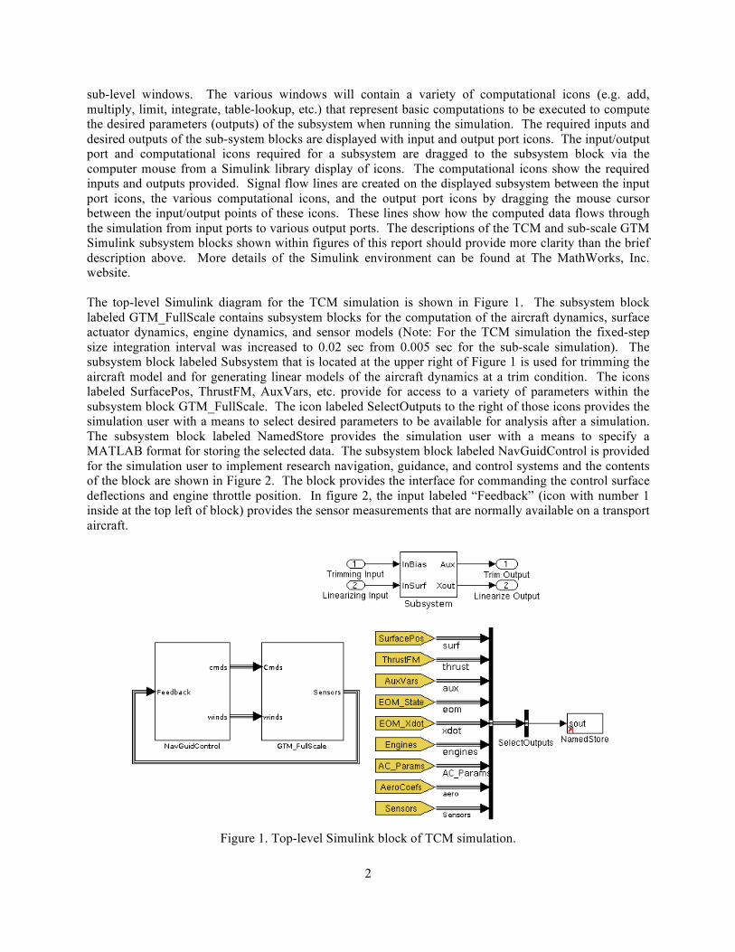
For the sub-scale GTM simulation, the contents of the Simulink block for the aerodynamic body coefficients (CX, CY, CZ, Cl, Cm, and Cn) and the aerodynamic forces and moments computation are shown in Figure 4. The output (C6) of the block labeled “Basic Airframe” is a 6x1 vector containing the body coefficients for the basic airframe. The outputs from the blocks labeled “Control Surface” and “Dynamic Derivatives” are incremental (delta) values of the body coefficients that add to the basic airframe coefficients to form the total aerodynamic body coefficients that are input to the block labeled “Coefficient Evaluation”, located at the right-center of the figure, to compute forces and moments.

C6 =

CX

CY

CZ

Cl

CM

CN

⎡

⎣

⎢⎢⎢⎢⎢

⎤

⎦

⎥⎥⎥⎥⎥

Figure 4. Sub-scale GTM Aero coefficient Simulink block.

The contents of the block GTM_FS_Aero of Figure 3 are shown in Figure 5. The Simulink blocks of Figure 5 compute the aerodynamic coefficients, forces, and moments for the TCM simulation. All of these blocks except the block labeled “Reynolds Number” were implemented by copying the sub-scale GTM simulation blocks shown in Figure 4 and then modifying the Basic Airframe and Control Surface blocks for input of the Reynolds number and adjusted aerodynamic data. The block “Reynolds Number” as shown at the top left was added to compute the Reynolds number as a function of altitude and Mach number. The subsystem block labeled “AeroBusLabel” shown at the upper right was added and this subsystem simply demuxes (splits) the six-element signal of aerodynamic coefficients, assigns a label to each one, and reassembles the labeled signals in a signal bus. With this addition, the names of the coefficients are visible downstream in the simulation. The contents of the Basic Airframe block (of Figure 4) for the sub-scale GTM simulation are shown in Figure 6. The block “Interpolation Using Prelookup” is a table lookup block that outputs the six body coefficients for the basic airframe. The two blocks at the top left of Figure 6, whose outputs are the first four inputs to the table lookup block, are companion pre-lookup blocks to the table lookup block that keep track of the breakpoints that were used for the previous computational iteration of table lookup values. This tracking of the lookup breakpoints by the pre-lookup blocks reduces computation time. The fifth input to the table lookup block with “(0:5)” inside the block allows the user to specify a range of output parameters that the block will output. Note that the first coefficient in the table lookup data array is indexed to zero. So, for the “(0:5)” input specification, all six coefficients are to be output (0 – CX, 1 - CY,

7

2 – CZ, etc.). The block “Interpolation Using Prelookup1” that is located at the middle, slightly left in Figure 6 computes delta values for the lateral coefficients and, when input 3 labeled “symmetry_on” is non-zero or true, these deltas are added to the basic airframe lateral coefficients to cause them to be symmetrical about the sideslip angle or beta. The block “DamageEffects” at the bottom of the Figure 6 computes increments to the basic airframe coefficients when the “damage_case” input to the block has a non-zero integer value to emulate damage to the airframe such as partial loss of the aircraft wing or vertical stabilizer.

Figure 5. Contents of TCM Simulink block labeled GTM_FS_Aero.

The contents of TCM modified “Basic Airframe” block (of Figure 5) is shown in Figure 7. One modification to this block from the sub-scale GTM block was to change the source of the data to be that stored in variable C4_bas.dat as defined in Appendix A. This variable contains the GTM polynomial database (table-lookup form) coefficient data for CY, Cl, Cm, and Cn as used by the sub-scale GTM simulation. A second modification was to specify the fifth input as (0:3) so that all of the available coefficients in C4_bas.dat would be output from the block. The block labeled “Interpolation Using Prelookup2” was added to determine the CX and CZ coefficients as a function of alpha, beta, and Reynolds number and the block labeled “Assignment CX CZ” was added to assign the CX and CZ coefficient to the correct positions of the 6x1 vector (C6) that contains the six basic airframe body coefficients. The blocks for lateral symmetry and damage effects remained the same as those for the sub-scale GTM simulation.

8

Figure 6. Contents of GTM Simulink block Basic Airframe.

Figure 7. Contents of TCM Simulink block Basic Airframe.

9

The contents of the block “Control Surfaces” for computing the aerodynamic coefficient increments due to control surface deflections for the sub-scale GTM simulation are shown in Figure 8 and the contents of the “Control Surfaces” block for the TCM simulation are shown in Figure 9. Note that the only difference between these figures is that the block labeled “Flaps” for the TCM simulation has a Reynolds number input. Note that each signal line output from the various blocks contain increments to the six aerodynamic coefficients due to a deflection of the control surface associated with the output signal line. For example, for the block labeled “Rudder”, the output signal line labeled “Upper” contains increments for CX, CY, CZ, Cl, Cm, and Cn as a result of deflecting the upper rudder surface. All the increments from the various surfaces and landing gear position are input to the block labeled “Implement Damage Models” where they are added together to produce the total of the increments to the six aerodynamic coefficients due to surface deflections and gear position that are contained in the output of the block (dC6). The block labeled “Implement Damage Models” will also modify the appropriate control surface increments for a specified missing control surface. Figure 10 shows the contents of the “Flaps” block for the sub-scale GTM simulation and Figure 11 shows the contents of the “Flaps” block for the TCM simulation. For the TCM simulation, the four “Flap Table” blocks were modified to have additional inputs of alpha and Reynolds number. Figure 12 shows the contents of a “Flap Table” block for the sub-scale GTM simulation where the block labeled “Interpolation Using Prelookup” computes increments to CX, Cm, and CZ due to flap deflection. The block labeled “Assignment to Longitudinal” then assigns these increments to a 6x1 vector of aerodynamic increments due to flap deflection where the lateral increments are zero. Figure 13 shows the contents of the “Flap Table” block for the TCM simulation. For the TCM simulation, the coefficient Cm due to flap deflection remained unchanged whereas CX and CZ due to flap deflection were modified to change as a function of Reynolds number. As a result, the computation for Cm and the computation for CX and CZ due to flap deflection were separated. Figure 13 shows that the blocks labeled “dC1_flp” and “Assignment to CM” were added to compute the unchanged Cm due to flap deflection. The “dC1_flp” block uses data from the variable dc1_flp computed by M-file dataconvert (see details of dataconvert in Appendix A). The block labeled “Interpolation Using Prelookup1” in Figure 13 was modified from that of Figure 12 to produce increments to CX and CZ as a function of Reynolds number, angle of attack, and flap deflection. This block uses the data stored in variable dc2_flp that is computed in M-file dataconvert.m (see dataconvert in Appendix A). All the sub-scale GTM simulation Simulink diagrams that were modified for development of the TCM simulation aerodynamic database calculations are shown in Figures 5, 7, 9, 11, and 13.

10

Figure 8. Contents of the sub-scale GTM Simulink block Control Surfaces.

11

Figure 9. Contents of the TCM Simulink block Control Surfaces.

12

Figure 10. Contents of Flaps Simulink block for GTM simulation.

Figure 11. Contents of Flaps Simulink block of TCM simulation.

13

Figure 12. Contents of Simulink Flap Table block for sub-scale GTM simulation.

Figure 13. Contents of Simulink Flap Table block for TCM simulation.

Definition of Geometry, Mass, and Inertia Parameters

The dimension parameters for the TCM simulation were scaled up based on the fact that the sub-scale model is a 5.5% model of a full-scale, mid-sized, single-aisle transport aircraft. Thus, the wing-span and mean aerodynamic chord of the full-scale transport were set to 1/0.055 times the subscale wing span and mean aerodynamic chord respectively. The wing area for the full-scale model was set to be (1/0.055)2 times the subscale wing area. The aircraft weight was set to 185,000 lbs that represents a mid-value weight for a mid-sized transport aircraft. The full-scale inertias chosen are representative values for the 185,000 lb weight. Roll inertia (Ixx) was set to 1,770,000 slug-ft2, pitch inertia (Iyy) to 5,680,000

14

slug-ft2, yaw inertia (Izz) to 7,270,000 slug-ft2, roll/yaw cross-inertia (Ixz) to 160,000 slug-ft2, pitch/yaw cross-inertia (Iyz) to 0, and roll/pitch cross inertia (Ixy) to 0. The center-of-gravity (CG) position was set to 25% of the mean aerodynamic chord. TCM Engine Model

The engine model used for the TCM simulation was developed at Glenn Research Center (GRC) and was implemented by GRC with Simulink software. The engine model is representative of a turbofan jet engine with a maximum sea-level thrust of approximately 40,000 lbs. The model is a simplified table lookup dynamic model referred to as Simp2. This model was developed using the GRC software tool called C-MAPSS40k that is a complete simulation of a turbo fan jet engine (Commercial Modular Aero-Propulsion System Simulation – ref. 6). The closed-loop dynamics of simp2 are modeled as a first-order system of the engine fan speed with a variable time constant. The time constant varies as a function of altitude and fan speed. The first-order system is driven by a desired fan speed that is a function of the Mach number, altitude, and throttle position. Pure time delays that vary as a function of fan speed, altitude, Mach number, and throttle position are added to the commanded throttle position to produce a throttle position that is also rate limited where the rate limit varies as a function of altitude. The model computes sea-level thrust as a function of the fan speed and the Mach number. Net thrust is computed as sea-level thrust times the pressure ratio (ratio of static pressure at altitude to sea-level static pressure). The model outputs the sea-level thrust, net thrust, model fan speed, and a corrected fan speed. The TCM simulation models two wing-mounted engines like the sub-scale GTM simulation. Thus, use of the simp2 engine model in the TCM simulation results in a maximum sea-level thrust of approximately 80,000 lbs. The simp2 model was implemented in the TCM simulation as a Simulink library model and is accessed in the block labeled GTM_FS_Engines shown in Figure 3. The contents of this block are shown in Figure 14. The contents of the block are like that for the GTM sub-scale simulation except for the contents of the top left two blocks labeled “Left_Engine Glenn_simp2” and “Right_Engine Glenn_simp2.” The contents of each block contain the Simp2 engine model. The six outputs from each engine block are net thrust (Thrust), engine RPM, (RPM), engine angular momentum (h), fuel flow (Fuel Flow), engine pressure ratio (EPR) and exhaust gas temperature (EGT). The Simp2 model only computes the first two outputs; so zero values are output for the last four outputs (Note: The six outputs from the engine blocks are typical outputs that could be provided by other engine models implemented in the blocks). For the Simp2 model, the corrected fan speed is the second output (RPM). In the center of Figure 14, the block labeled “Engine Alignment” computes the aircraft body axes components of the left and right engine thrust (vectors TL and TR), the total thrust components (vector T that is the sum of TL & TR), and engine angular moment body axes components (vector H). The block labeled “CG torque” computes body axes torques due to engine thrust. The block labeled “3D Vector Cross Product” computes body axes torques due to the angular moment components. Below the “Right Engine” block are blocks that compute an output called Bypass that is input to both engine blocks. When Bypass is true, the engine model state is bypassed. Bypass is true when trimming the model or when linear aircraft dynamic models are computed. The blocks at the bottom of Figure 14 compute a fuel used quantity. These blocks were implemented for the sub-scale GTM simulation and while fuel used was not modeled in Simp2, the blocks were not removed to minimize changes from the sub-scale GTM simulation. The remaining icons at the lower right of Figure 14 create the output (Engines) of engine parameters that are available to the simulation user at the top-level Simulink block of the TCM simulation. Modifications were made to the Simp2 engine model received from GRC. One modification was to replace the Simulink library table lookup blocks with Simulink library “Interpolation Using Pre-lookup” and “pre-lookup” companion blocks. This modification was done to increase the execution speed of the model. Another modification was to change the method for initializing the one engine state of the model that represents the modeled engine fan speed. The change was to initialize the engine state with the

15

commanded fan speed at time zero as computed by the Simulink interpolation and pre-lookup blocks rather than with a value pre-computed in an M-file as it was in the model received from GRC. This changed was made ensure that the initial engine state value would be the same as the initial value from the Simulink table lookup blocks. The initial value from the M-file was computed with the MATLAB table lookup function interp3 using table data that was a thinned-version of the table lookup data used by the Simulink table lookup blocks and that resulted in the interp3 value being different than the initial value computed by the Simulink table lookup blocks. Another modification was to add blocks to the model for converting the TCM throttle position that has units of percent throttle to the Simp2 model throttle position in degree units. A further modification was to insert two Simulink Memory blocks in two signal paths of the Simp2 model block that computes the commanded throttle position time delays and rate limiting. The Memory blocks were added to eliminate algebraic loops that occurred during trimming and linearization of the aircraft model. A final modification was to change the Simp2 initialization M-file named simp2_model_parameters.m so that the computed engine parameters would be stored in the Simulink model workspace rather than in the MATLAB workspace.

Figure 14. Contents of Simulink GTM_FS_Engine block for the TCM simulation.

16

Full-Scale Surface Actuators

Surface actuator models were developed for the TCM simulation to have response times and non-linear characteristics that are representative of full-scale transport aircraft rather than a particular transport aircraft. These models were developed based on information found in references 7 and 8. None of the models developed are exactly like any of the models described in the references above. Instead, the data in the references was used as a guide to produce models that have representative non-linear characteristics. None of the sub-scale GTM simulation actuator models were used for the TCM simulation because those models have a much faster response than the response of transport aircraft actuators and do not account for some non-linear characteristics present on full-scale transport aircraft. The non-linear characteristics typical for full-scale transport aircraft are variable rate limiting, variable position blow-down limits (the surface position limits where the force produced by the actuator is balanced by the aerodynamic force on the surface acting through actuator gearing), and hysteresis. Hysteresis was not included in any of the models since a non-proprietary source was not located for the values of the hysteresis. In addition, the stabilizer and flap dynamics of full-scale transport aircraft are much different than the stabilizer and flap position actuation dynamics of the sub-scale GTM simulation. For the sub-scale GTM simulation, the stabilizer and flap actuator models are like the elevator, aileron, rudder, and spoiler actuator models; that is, they were modeled as first order lags with fixed position limits and fixed rate limits. For transport aircraft, stabilizer and flap actuation is normally accomplished using ball screw actuators that slowly move the stabilizer and flap surfaces. Normally, the stabilizer is only used for pitch trim and the flap position changes when the pilot moves a flap handle to different discrete detent positions as a function of the flap speed ranges specified in the aircraft’s pilot hand book. So, for the TCM simulation, the stabilizer and flap actuator models were developed to be representative of position movement for ball screw actuation. In the TCM simulation, the block labeled GTM_FS_Actuators of Figure 3, contains a block labeled “Actuator_Dynamics” that contains all of the surface actuator models. All the actuator models for the TCM simulation were implemented as Simulink library models. The use of library models allows multiple copies of an actuator model to be easily implemented within a Simulink simulation by dragging copies of the library model into the simulation blocks. The contents of “Actuator_Dynamics” block are shown in Figure 15. The total surface position commands are computed in this block given the trim surface positions (bias.elevator, bias.aileron, etc.) and the surface commands relative to those trim positions. Block “ElevatorActuators” contains four independent identical actuator models for the left and right in-board elevator surfaces and the left and right outboard elevator surfaces. Note that full-scale transport aircraft only have left and right elevator surfaces that are not normally independently controlled. However, for research purposes, the four elevator surfaces were used just like the sub-scale GTM simulation model. The block labeled “AileronActuators” contains two independent actuator models for the left and right aileron surfaces. The block labeled “RudderActuators” contains two independent actuator models for the upper and lower rudder surfaces (some transport aircraft only have one rudder surface). The block labeled “SpoilerActuators” contains four independent actuator models for the left and right in-board spoiler panels and the left and right outboard panels (some full-scale transport aircraft have five spoiler panels on the left wing and five on the right wing). The block labeled “FlapPCU_FS” contains one actuator model whose output drives the four flap surfaces contained in the GTM aerodynamic model. If research needs were to arise for independent control of the four modeled flap surfaces, actuators could be easily added to the block. The block labeled “StabPCU_FS” contains one actuator model for control of the stabilizer surface. The details of each TCM actuator are discussed in the following subsections.

17

Figure 15. Contents of the Actuator_Dynamics Simulink block for TCM simulation.

18

Elevator Actuator

The elevator actuator for the TCM simulation is modeled as a first-order lag having a bandwidth of 31.8 deg/sec (20 radians/sec) and with rate and position limits that are variable. The rate limit varies as a function of the actuator position and the position limit varies as a function of equivalent airspeed. The rate limits have a no-load value when the surface is at its centered or neutral position. The rate limit decreases as the surface moves away from the neutral position since the force due to dynamic pressure, that opposes the surface deflection, increases with increasing deflection of the surface position. The rate approaches the minimum as the surface approaches maximum deflection. The maximum rate occurs when the surface is being commanded toward neutral when the surface position is at the maximum deflection (when the deflection of the surface position is decreasing, the force due to dynamic pressure is adding to the force of the actuator and thus assisting in decreasing the deflection of the surface position). Figure 16 shows the contents of the Simulink block for the elevator actuator where the integrator of the actuator servo loop is in block “VarLimIntegIC”. The maximum positive and minimum negative position-limits are input to block “BlowDownLimits” and are set during simulation initialization. These limits are modified as a function of equivalent airspeed (EAS, knots) in block “BlowDownLimits” shown in Figure 17. The blow-down limits are a rough approximation to those found in transport simulator models (for example, see reference 7). The variable actuator rate limits are computed in Simulink block “VarRateLmit” as shown in Figure 18. The rate varies between 35 and 65 deg/sec depending on the surface position and the direction in which the surface is moving. The maximum is typical of transport servo actuators (see, for example, ref. 8). The positive and negative rate limits are computed in the two table lookup blocks at the left side of the figure and the block labeled “Saturation Dynamic” applies these limits to the rate signal. The contents of Simulink block “VarLimIntegIC” are shown in Figure 19. This block initializes the integrator output to the commanded input at simulation time 0 and limits the integrator output to the positive and negative variable position limits that are input to the block. This implementation will prevent the integrator output from exceeding the limit and will reduce the integrator output if the integrator is on the limit and the magnitude of the limit decreases. This implementation works well for limits that vary smoothly, but does not work properly for limits with large step changes. This block was used as well for the aileron, rudder, and spoiler actuator models. Note that rate output from block VarRateLimit does not go to zero at the position limits. However, the rate input to the integrator in block VarLimIntegIC does go to zero at the position limits.

Figure 16. Contents of elevator actuator Simulink block for TCM simulation.

19

Figure 17. Contents of BlowDownLimits Simulink block for TCM simulation.

Figure 18. Contents of VarRateLimit Simulink block for TCM simulation.

Figure 19. Contents of VarLimIntegIC Simulinkblock for TCM simulation.

20

Aileron Actuator

The aileron actuator is modeled as a first-order lag with fixed position limits and variable rate limiting. Figure 20 shows the contents of Simulink block labeled “AileronActuators” shown in Figure 15. The top two blocks contain identical aileron actuator models for the deflecting the left and right aileron surfaces. The gain block labeled “SplRollCoupling” acts as a switch to turn on or turn off the coupling of the commanded spoiler position to the aileron command. This switch was originally implemented for the GTM sub-scale simulation for investigating roll control performance with and without the spoilers. For full-scale aircraft this coupling is always present for normal operation to achieve desired roll performance. For full-scale aircraft, when the aircraft is commanded to roll, the spoilers on the down-wing are commanded up as a function of the commanded aileron deflection. Figure 21 shows the contents of Simulink block AilPCU_FS that is the TCM simulation aileron actuator model. The aileron model has fixed upper and lower position limits that are set during initialization of the simulation in variable Act.AilPL that is accessed by the block at the top left of Figure 21. During early development of the aileron actuator model, position limits that varied as a function of equivalent airspeed like that for the elevator actuator model were considered. So, the input of equivalent airspeed shown as input 2 (EAS) of Figure 21 was implemented. However, the available reference information showed that the surface blowdown of the ailerons was much less than that for the elevator and a simple implementation of constant position limiting was chosen for the aileron actuator model. Thus, the EAS input was just terminated with a Simulink termination block rather than removing the input. The contents of the block “VarRateLimit” are shown in Figure 22. The magnitude of the rate limit varies between 40 and 69 deg/sec depending on the actuator output position and the direction that the surface position is moving. The aileron rate limit behaves like that described earlier for the elevator rate limit.

Figure 20. Contents of Simulink block AileronActuators for the TCM simulation.

21

Figure 21. Aileron actuator model contained in both Simulink blocks AilPCU_FS and AilPCU_FS1 for TCM simulation.

Figure 22. Contents of VarRateLimit block for aileron actuator model of TCM simulation.

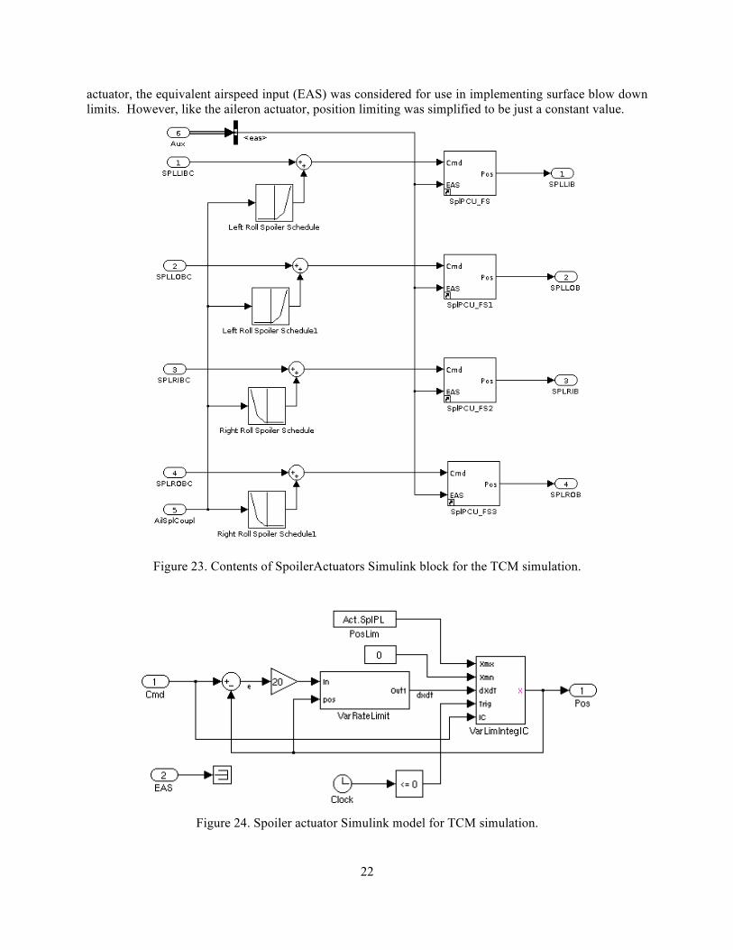
Spoiler Actuator

The spoiler actuators are modeled as a first-order lag with variable position and rate limiting. The simulation contains four identical spoiler actuator models for the four spoiler surfaces in the aerodynamics model – two on the right wing and two on the left wing. The block labeled “SpoilerActuators” shown in Figure 15 contains the four actuator models and blocks to compute the spoiler actuator commands due to aileron commands (aileron/spoiler coupling). The inputs to this block are four surface commands (where each command is a delta command from trim plus the trim spoiler position (bias.speedbrake)), the aileron-coupling command, and an input labeled “Aux” containing auxiliary variables (CAS, EAS, etc.). The contents of the SpoilerActuators block are shown in Figure 23. The four blocks on the left side of the figure compute spoiler deflection commands as a function of the coupled aileron command. The table lookup data in these blocks was chosen to produce a roll control torque that is approximately linear with the commanded aileron deflection. The four blocks to the right of the table lookup blocks each contain an identical spoiler actuator model. Figure 24 shows the spoiler actuator Simulink model. The maximum spoiler deflection is specified in variable Act.SplPL and the minimum spoiler deflection is zero. The rate limit varies between 61 and 89 deg/sec as a function of the actuator position and the direction the surface is moving. At the initial development of the spoiler

22

actuator, the equivalent airspeed input (EAS) was considered for use in implementing surface blow down limits. However, like the aileron actuator, position limiting was simplified to be just a constant value.

Figure 23. Contents of SpoilerActuators Simulink block for the TCM simulation.

Figure 24. Spoiler actuator Simulink model for TCM simulation.

23

Rudder Actuator

Two identical rudder actuators are modeled for the upper and lower rudder surface inputs to the aerodynamics database. Figure 25 shows the rudder actuator Simulink model. The actuator is modeled as a first-order lag with variable rate limits. The rudder command is input to the “RudderRatioChanger” block that multiplies the rudder command by a gain that varies from 1 to 0.1 as the speed increases. A rudder ratio changer is used on some transport aircraft to ensure that the rudder deflection does not exceed load limits if a large rudder command were to occur. The “YawDamper” block is a place-holder block where a yaw damper model would be implemented as a parallel command. On transport aircraft that have the rudder pedals connected to the actuators with mechanical cables, the yaw damper command is mechanically added in parallel to the rudder command to prevent the yaw damper commands from back-driving the rudder pedals. The contents of the block “VarRateLimit” are shown in Figure 26. The rate limits vary between 10 and 90 deg/sec depending on the actuator position and the direction the actuator is moving.

Figure 25. Rudder actuator Simulink model for TCM simulation.

Figure 26. Contents of rudder actuator Simulink block VarRateLimit for the TCM simulation.

Stabilizer Actuator

The stabilizer actuator model for the TCM simulation is modeled according to transport aircraft that use the stabilizer (horizontal tail) for pitch trim. For these aircraft, the stabilizer is positioned by a ball screw actuator that is normally driven by two hydraulic or electric motors. The two motors are connected in a

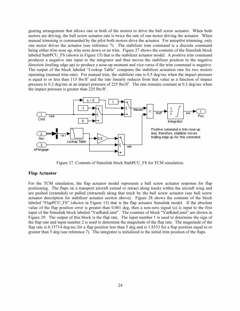
24

gearing arrangement that allows one or both of the motors to drive the ball screw actuator. When both motors are driving, the ball screw actuator rate is twice the rate of one motor driving the actuator. When manual trimming is commanded by the pilot both motors drive the actuator. For autopilot trimming, only one motor drives the actuator (see reference 7). The stabilizer trim command is a discrete command being either trim nose up, trim nose down or no trim. Figure 27 shows the contents of the Simulink block labeled StabPCU_FS (shown in Figure 15) that is the stabilizer actuator model. A positive trim command produces a negative rate input to the integrator and thus moves the stabilizer position in the negative direction (trailing edge up) to produce a nose-up moment and vice-versa if the trim command is negative. The output of the block labeled “Lookup Table” computes the stabilizer actuation rate for two motors operating (manual trim rate). For manual trim, the stabilizer rate is 0.5 deg/sec when the impact pressure is equal to or less than 115 lbs/ft2 and the rate linearly reduces from that value as a function of impact pressure to 0.2 deg/sec at an impact pressure of 225 lbs/ft2. The rate remains constant at 0.2 deg/sec when the impact pressure is greater than 225 lbs/ft2.

Figure 27. Contents of Simulink block StabPCU_FS for TCM simulation.

Flap Actuator

For the TCM simulation, the flap actuator model represents a ball screw actuator response for flap positioning. The flaps on a transport aircraft extend or retract along tracks within the aircraft wing and are pushed (extended) or pulled (retracted) along that track by the ball screw actuator (see ball screw actuator description for stabilizer actuator section above). Figure 28 shows the contents of the block labeled “FlapPCU_FS” (shown in Figure 15) that is the flap actuator Simulink model. If the absolute value of the flap position error is greater than 0.001 deg, then a non-zero signal (e) is input to the first input of the Simulink block labeled “VarRateLimit”. The contents of block “VarRateLimit” are shown in Figure 29. The output of this block is the flap rate. The input number 1 is used to determine the sign of the flap rate and input number 2 is used to determine the magnitude of the flap rate. The magnitude of the flap rate is 0.15714 deg/sec for a flap position less than 5 deg and is 1.8333 for a flap position equal to or greater than 5 deg (see reference 7). The integrator is initialized to the initial trim position of the flaps.

25

Figure 28. Flap actuator Simulink model for the TCM simulation.

Figure 29. Flap actuator Simulink rate limit model for TCM simulation.

Trimming

Trimming the TCM simulation can be accomplished in two ways. One way is to edit the simulation initialization M-file setupFS.m to specify the user’s desired trim condition and then execute this M-file. Execution of setupFS.m re-initializes the simulation if setupFS.m was not previously executed, calls the trim M-file trimgtm.m (written as a MATLAB function), and loads the trimmed values into the Simulink simulation model workspace. The model can also be trimmed to new conditions by executing the trim M-file trimgtm.m after setupFS.m has been previously executed. When trimming with setupFS.m, a desired trim condition is specified in setupFS.m by setting values for the variables cas (calibrated airspeed in knots), altitude (altitude in feet), roll (roll attitude in deg), gamma (flight path angle in deg), yaw (heading in deg), MWS.bias.flaps (flap position in deg), and MWS.bias.geardown (gear position, 1 down, 0 up). When using trimgtm.m to determine new trim values, the trim flap and gear position cannot be specified in the calling arguments of trimgtm.m and trimming will occur with the flap and gear values that were last specified during execution of setupFS.m. Also, trimgtm.m does not load the trim values into the Simulink model workspace whereas setupFS.m does. If the user wants to run the simulation with the trim values computed with trimgtm.m, the M-file loadwms.m must be run to load the trim values into the simulation model workspace. The M-file trimgtm.m that is used for the TCM simulation is a slightly modified version of the M-file that was developed for trimming the sub-scale GTM simulation. The only modifications were to (1) change some block name references to those of the full-scale simulation, (2) set some initial conditions for some block values unique to the full-scale simulation, (3) set a different value for the initial guess on the throttle position, and (4) set simulation time values to be integer multiples of the 0.02 sec fixed integration time step used for the full-scale simulation (the sub-scale GTM simulation uses a 0.005 sec fixed integration time step). Appendix B shows the trim data output to the MATLAB command window after the model is trimmed.

26

Linearization

Linear models about trim conditions for the TCM are readily generated using the M-file function linmodel.m that was developed at LaRC for the sub-scale GTM simulation. This sub-scale M-file was modified slightly for use in the TCM simulation. The modifications were to change the sub-scale GTM simulation model name references to TCM simulation model name references. Execution of this file computes a MATLAB state space system of A, B, C and D matrices for the 12 states of the six degree-of-freedom aircraft dynamics model, 19 control inputs and 15 outputs. The states, control inputs, and computed outputs are listed in Appendix C. Also computed are separate longitudinal and lateral linear dynamic models that are extracted from the A, B, C, and D matrices above. The separate longitudinal and lateral models can be generated with all the control inputs or with a reduced set of control inputs (see Appendix C for details). The setting of a flag also provides for computation of longitudinal and lateral linear models in the stability axes (see Appendix C for details). Example M-File Scripts

Within the TCM simulation software package, there are four M-files that provide examples of what can be done with the TCM simulation and provide check cases for a user to determine if the simulation was correctly installed on a computer system. The names of the four M-files are example1FS.m, example2FS.m, example3FS.m, and example4FS.m. These M-files are modified versions of the M-files example1.m, example2.m, example3.m, and example4.m that were developed at LaRC for the sub-scale GTM simulation. A brief description of each of these files follows and further details of the data and plots produced by these running these M-files can be found in Appendix D. The M-file example1FS.m trims the TCM simulation transport aircraft model to level flight at an altitude of 15000 ft and a calibrated airspeed of 260 knots with the flaps and gear up. The script computes the linear model for this trimmed condition and then computes an elevator, rudder, and aileron doublet response for both the linear and non-linear simulation models. Finally, the doublet responses are co-plotted so that they can be compared. The M-file example2FS.m trims the aircraft model in level flight at an altitude of 10,000 ft with the flaps and gear up for four calibrated airspeed and four angle-of-attack conditions. Then, two plots are made of these results. One plot shows the trimmed stabilizer position, throttle position, and angle of attack as a function of calibrated airspeed and the second plot shows the trimmed stabilizer position, throttle position, and calibrated airspeed as a function of angle of attack. The M-file examle3FS.m trims the aircraft model in level flight at an altitude of 10,000 ft with the flaps and gear up for five angle-of-attack values (2, 4, 6, 8, and 10 deg) and computes linear models for these trim conditions. Then, the phugoid and short period frequency and damping of the longitudinal dynamics are computed for each linear model. Finally, four plots are made – (1) phugoid mode frequency versus angle of attack, (2) phugoid mode damping versus angle of attack, (3) short period mode frequency versus angle of attack, and (4) short period mode damping versus angle of attack. The M-file example4FS.m first trims the non-linear aircraft model in a climbing turn where the flight path angle is 3 deg, the roll attitude (bank angle) is 25 deg, calibrated airspeed is 200 knots, altitude is 10,000 ft, flaps are 5 deg, and the landing gear is up. Next, a linear aircraft model is found for this trim condition. Then, three 60-sec simulation runs are made with the controls commanded to trim values. The first simulation is with the non-linear aircraft model starting from the trim condition. The second simulation is like the first simulation except that prior to running the simulation, the angle of attack is offset from the trim angle of attack by 2 degrees. The third simulation is the same as the second

27

simulation except that the third simulation uses the linear aircraft model in place of the non-linear aircraft model. Finally, a 3D plot is made for the three resulting simulation trajectories of altitude versus latitude and longitude. Simulation Validation

This section describes what was done to validate the TCM simulation as a scaled-up simulation of the sub-scale GTM simulation. Validation was accomplished by comparing the GTM simulation responses for commanded elevator, aileron, and rudder doublets with those responses from the TCM simulation. The TCM doublet responses were scaled according to the scaling relationships defined by the scale factor of the sub-scale model relative to the full-scale model to compare the responses. (See ref. 9 for scaling relationships.) The commanded doublets for the GTM simulation were simulated for a trim condition of 75 knots true airspeed, altitude of 500 ft, weight of 49.6 lbs, level flight, flaps up, and gear up. The commanded doublets for the TCM simulation were computed for a trim condition of 319.8 knots true airspeed, altitude of 15,000 ft, weight of 190,431.3 lbs, level flight, flaps up, and gear up. The TCM trim true airspeed was scaled from the GTM trim true speed equal to 75 divided by the square root of GTM model scale factor of 0.055 or 0.235 (ref. 9). The TCM trim weight was scaled from the GTM trim weight as atmospheric density of the TCM divided by atmospheric density of the GTM times 49.6 divided by the cube of the GTM model scale factor. Each TCM moment of inertia for the doublet response comparison was computed from the respective GTM moment of inertia as atmospheric density of the TCM divided by atmospheric density of the GTM times the GTM moment of inertia divided by the 5th power of the GTM model scale factor. The full scale TCM commanded surface position doublets were all the same magnitude and duration. The magnitude of the doublets was 2 deg. The duration of the positive and negative pulses that make up the doublet was 1 s. Each doublet was simulated independently with a doublet starting with a positive pulse at 1 sec followed by the negative pulse at 2 s. The sub-scale GTM commanded surface position doublets were scaled versions of the TCM doublets. The magnitude of the pulses remained the same since angles scale one-to-one between the subscale and fullscale models (ref. 9). The duration of the pulses for the GTM were scaled by the square root of the subscale model scale factor of 0.055 or 0.235; that is, the pulse duration for the subscale was 0.235 s versus 1 sec. for the full scale model. The subscale doublets were simulated independently and each began at 1 s. The commanded doublets were input to the surface actuator models of the simulations. The bandwidth of the subscale surface actuators was modified to be the scaled bandwidth of the full-scale actuators. The bandwidth of the full-scale actuators was modeled, as stated in the Full-Scale Surface Actuators section of this report, at 20 rad/s or 3.183 Hz that is a realistic value for hydraulic actuators. So, for the doublet response comparison, the scaled bandwidth for the sub-scale actuators was set to 3.183 divided by 0.235 (square root of model scale factor) or 13.57 Hz. That compares to the bandwidth of the surface actuator models in the unmodified GTM simulation which is modeled at 5 Hz. That bandwidth represents the highest bandwidth availiable for electomechanical actuators of the size used in the hardware GTM subscale model. The TCM simulation was run three times to generate dynamic responses for the commanded elevator, aileron, and rudder doublets described above and the response data were saved to a file for each run. Then, the GTM simulation was run three times to generate the dynamic response for its commanded elevator, aileron, and rudder doublets. After each GTM simulation, the corresponding saved TCM data file was loaded and then scaled for comparison with the GTM response. The TCM time and angular rate data were multiplied by the factor 0.235 (square root of sub-scale model scale factor of 0.055). In

28

addition, after the TCM time was multiplied by 0.235 it was shifted by 1 minus 0.235 s or 0.765 s to align the TCM scaled responses with the GTM responses. Then, the GTM and scaled TCM responses were co-plotted for comparison. Figure 30 shows the response data for the commanded elevator doublet. The plot of body pitch rate shows an excellent match between the GTM pitchrate response and the scaled TCM response. Small offsets are shown for the GTM pitch and scaled TCM pitch and the GTM angle of attack and the scaled TCM angle of attack. The amount of offset is attributed to the Reynolds number correction to the subscale lift coefficient. The plot of elevator position shows excellent agreement between the GTM elevator position and scaled TCM elevator position. Figure 31 shows the response data for the command aileron doublets and Figure 32 shows the response data for the commanded rudder doublets. As can be seen by the plotted data, there is excellent agreement for all plotted parameters of these doublet responses.

Figure 30. Overlaid response data for GTM and TCM elevator doublets.

29

Figure 31. Overlaid response data for GTM and TCM aileron doublets.

30

Figure 32. Overlaid response data for GTM and TCM rudder doublets.

Concluding Remarks

A generic, non-proprietary, twin-jet, under-the-wing, transport aircraft simulation, named Transport Class Model (TCM), was developed using the Simulink simulation environment for the purpose of performing controls research at potentially extreme attitudes to address transport aircraft safety issues such as loss-of-control due to inadvertant stalls, environment disturbances, or aircraft system failures. The development of the TCM started with a sub-scale tranport model simulation named the Generic Transport Model (GTM) simulation (implemented within Simulink environment) that models a flyable remotely-controlled Unmanned Aerial Vehicle (UAV) developed at LaRC. Modifications were made to the GTM simulation to develop the TCM simulation. Modifications included appropriate scaling of the GTM dimension parameters to produce TCM values for wing span and surface area, wing chord length, CG location, and engine location. The TCM weight and moments of inertia were selected to be representative of a mid-weight, twin-jet transport aircraft. Other

31

modifications included new surface position acturator models, a new engine model, and modification of the lift and drag coefficients of the GTM aerodynamic database. The new surface position actuator models of the TCM simulation are representative of hydraulic actuators instead of the electromechnical surface position actuators models of the GTM simulation. The hydraulic actuator models also included variable rate limits and the elevator actuator model also included variable positions limits. The stabilizer and flap actuator models for the TCM simulation were implemented to be representative of jackscrew actuated surfaces (low-rate actuated surfaces) rather than the hydraulic actuator models used for the elevator, aileron, spoilers, and rudder surfaces or the electromechical actuation models of the GTM simulation. A non-proprietary jet engine model (named Simp2), that was developed at Glenn Research Center and is representative of a 40,000 lb sea-level thrust engine, was integrated into the TCM simulation to replace the GTM engine model that was based on bench-tests of a small jet engine used on the flyable remote-controlled GTM aircraft. Simp2 is a first-order engine model of the engine fan speed where the time constant of the fan speed response is variable and changes as a function of altitude and fan speed. The engine thrust is a function of engine fan speed and Mach number. The lift and drag coefficients of the TCM simulation are modified versions of the lift and drag coefficients of the GTM aerodynamic database. The coefficients are modified by Reynolds numbers adjustments that are computed by table lookup as a function of altitude and Mach number when running the simulation. The Reynolds number adjustments for the lift and drag coefficients were developed at Ames Research Center. All the other aerodynamic coefficients of the TCM simulation remained the same as those of the GTM simulation. Finally, by comparing the commanded elevator, aileron, and rudder doublet responses for the TCM and GTM simulations by means of scale-model relationship factors, the scaled version of the simulated TCM dynamics were shown to be in good agreement with the GTM dynamics.

32

Appendix A – TCM Aerodynamic Database

Kaneshige Data

The Kaneshige database, used for definition of the TCM Cx and Cz aerodynamic body coefficients, were provided to LaRC in nine text data files shown in first column of the table below. The first three files listed below are for table lookup of Reynolds number as a function of altitude and Mach number. The next four files are used for table lookup of the flap component of Cx and Cz as a function of flap position, Reynolds number, and aerodynamic angle of attack. The fifth, eight, and ninth files are used for table lookup of the basic Cx and Cz as a function of Reynolds number, aerodynamic angle of attack, and aerodynamic sideslip angle. The text data files were converted to MATLAB® data by loading the text files into the MATLAB variables shown in column 3 of the table below with the MATLAB “load” command*. The dimensions of the MATLAB variables are shown in column 4. The MATLAB variables were stored in a MATLAB binary data file named gtmFS.mat for subsequent use by M-file dataconvert.m that creates the MATLAB aerodynamic database for the TCM simulation. Note that the breakpoint data for angle of attack (alpha) and sideslip angle (beta) for the Kaneshige database were not provided in text files since this breakpoint data is the same as that for the GTM subscale polynomial aerodynamic database. The MATLAB names for the alpha and beta breakpoint data are shown in the last two lines of the table. Table: Conversion of Kaneshige Files.

Text Data File Name Type File MATLAB Variable Name

MATLAB Variable Dimension

gtm_alt.dat breakpoint gtmAlt 1x5 array gtm_mach.dat breakpoint gtm_mach 1x9 array gtm_reynolds.dat table gtm_reynolds 9x5 array gtm_fullscale_flap.dat breakpoint gtmFS_flap 1x7 array gtm_rn.dat breakpoint gtm_rn 1x6 array gtm_fullscale_dC3_flp_cz.dat table gtmFS_dC3_flp_cz 192x7 array gtm_fullscale_dC3_flp_cx.dat table gtmFS_dC3_flp_cx 192x7 array gtm_fullscale_C6_bas_cz.dat table gtmFS_C6_bas_cz 192x27 array gtm_fullscale_C6_bas_cx.dat table gtmFS_C6_bas_cx 192x27 array breakpoint C6_bas.alpha 1x32 array breakpoint C6_bas.beta 1x27 array MATLAB M-File dataconvert.m

The MATLAB M-file named dataconvert.m was written to (1) read the data file gtmFS.mat, (2) read the GTM subscale polynomial aerodynamic database MATLAB file named T2_polynomial_aerodatabase.mat, (3) form 3-dimensional arrays from 2-dimension Kaneshige CX/CZ arrays, (4) extract the CY, Cl, Cm, and Cn data from the subscale polynomial aerodynamic database, and (5) store the manipulated data as the TCM aerodynamic database in file GTM_FS_aerodatabase.mat.

* MATLAB® is a registered trademarks of The MathWorks, Inc.

33

The M-file dataconvert.m script that was used to form the TCM aerodynamic database follows: % m-file dataconvert % % This script used to convert John Kaneshige "full scale GTM" % two-dimensional data files to three-dimensional data files % % Kaneshige data from file gtmFS.mat in directory % Desktop/GTMSimulink/FullScaleGTM_Kaneshige and GTM polynomial % aero data base in libs folder for the gtm_design simulation model; that % is, T2_polynomial_aerodatabase.mat % % R.M. Hueschen - 19May09 % path('../../FullScaleGTM_Kaneshige',path); % load('gtmFS'); % Kaneshige CX/CZ database % load('T2_polynomial_aerodatabase') % Convert Kaneshige C6_bas_cx 192x27 to 6X32X27 array m = 0; for i = 1:6 for j = 1:32 m = m + 1; for k = 1:27 GTM_FS_C6_bas_cx(i,j,k) = gtmFS_C6_bas_cx(m,k); end end end % % % Convert Kaneshige C6_bas_cz 192x27 to 6X32X27 array m = 0; for i = 1:6 for j = 1:32 m = m + 1; for k = 1:27 GTM_FS_C6_bas_cz(i,j,k) = gtmFS_C6_bas_cz(m,k); end end end % % % Convert Kaneshige C6_flp_cx 192x7 to 6X32X7 array m = 0; for i = 1:6 for j = 1:32 m = m + 1;

34

for k = 1:7 GTM_FS_dC3_flp_cx(i,j,k) = gtmFS_dC3_flp_cx(m,k); end end end % % Convert Kaneshige C6_flp_cz 192x7 to 6X32X7 array m = 0; for i = 1:6 for j = 1:32 m = m + 1; for k = 1:7 GTM_FS_dC3_flp_cz(i,j,k) = gtmFS_dC3_flp_cz(m,k); end end end % % Extract CY, Cl, Cm, and Cn data % C4_bas.data=C6_bas.data(:,:,[2 4 5 6]); C4_bas.alpha = C6_bas.alpha; C4_bas.beta = C6_bas.beta; C4_bas.dim = 'Dimensions are: [alpha_vec] x [beta_vec] x [CY Cl Cm Cn]'; % % Extract flap Cm data % dC1_flp.data=dC3_flp.data(:,:,3); dC1_flp.alpha = dC3_flp.alpha; dC1_flp.flap = dC3_flp.flap; dC1_flp.dim = 'Dimensions are: [alpha_vector] x [flap_vector] x [Cm]'; % % Form CX and CZ table lookup data from Kaneshige data % C2_bas.data(:,:,:,1) = GTM_FS_C6_bas_cx; C2_bas.data(:,:,:,2) = GTM_FS_C6_bas_cz; C2_bas.reyn = gtm_rn; C2_bas.alpha = C6_bas.alpha; C2_bas.beta = C6_bas.beta; C2_bas.dim = 'Dimensions are: [reynolds_vec] x [alpha_vec] x [beta_vec] x [CX CZ]'; % % Form flap CX and CZ table lookup data from Kaneshige data % dC2_flp.data(:,:,:,1) = GTM_FS_dC3_flp_cx; dC2_flp.data(:,:,:,2) = GTM_FS_dC3_flp_cz; dC2_flp.reyn = gtm_rn; dC2_flp.alpha = C6_bas.alpha; dC2_flp.flap = gtmFS_flap; dC2_flp.dim = 'Dimensions are: [reynolds_vec] x [alpha_vec] x [flap_vec] x [dCX dCZ]'; % Reyn.data = gtm_reynolds; Reyn.mach = gtm_mach;

35

Reyn.alt = gtmAlt; % ver = 'GTM Full Scale polynomial aero database with damage'; % save GTM_FS_aerodatabase C4_bas C2_bas dC1_flp dC2_flp dC3_p dC3_r dC6_ail dC6_rud dC6_w ... dC3_ele dC3_lgr dC3_q dC6_damage dC6_spo Reyn ver % save kaneshige3dimMats GTM_FS_C6_bas_cx GTM_FS_C6_bas_cz ... GTM_FS_dC3_flp_cx GTM_FS_dC3_flp_cz %

36

Validation of MATLAB Aero Data

A Simulink® model named Test_GTM_FS_Aero.mdl was constructed to validate the Simulink table lookup blocks used to generate the aerodynamic parameter values*. The M-file testFSaero.m (M-file script shown in following report section) was written to load the TCM and sub-scale GTM polynomial databases and compute the aerodynamic parameters as a function of aerodynamic angle of attack (alpha) with sideslip (beta) equal to zero using Simulink model Test_GTM_FS_Aero.mdl. The M-file plot script pltestFSaero.m (see report section M-file pltestFSareo.m) was written to plot the computed data. The plots of the basic airframe lift, drag, and pitching moment coefficients are shown in Figure 33 below. Note that “fullscale” in the plot labels is the TCM data for a Reynolds number correction at Mach number 0.3422 and altitude of 5000 ft and “T2 Poly” is the GTM subscale data. Note also that the Reynolds number correction used to generate the TCM data is most noticeable for the lift coefficient in the angle of attack (alpha) range of 10 to 25 deg. The plots of the lift and drag coefficients due to flap deflection are shown below in Figure 34. The plotted data compares well to data plots provided by ARC (ref. 2).

Figure 33. Lift, drag, and pitching moment coefficients as a function

of angle of attack for the TCM and sub-scale GTM polynomialdatabases (Reynolds number correction for TCM at Mach 0.3422 and altitude 5000 ft).

* Simulink®is a registered trademark of The Mathworks, Inc.

37

Figure 34. Lift and drag coefficients as a function of angle of attack for the TCM simulation.

M-File testFSaero.m

% testFSaero % % This m-file runs Simulink model Test_GTM_FS_Aero.mdl that was created from % blocks within the GTM_FS_aerodatabase.mdl library. % path('../libs',path); % d2r = pi/180.; % Load the GTM sub-scale aero database % AeroGTM = load('T2_polynomial_aerodatabase');

38

% Load the GTM full-scale aero database % Aero = load('GTM_FS_aerodatabase'); %This file in libs folder symmetric_aero_on = 1; flap = 0.; beta = 0.; dum1 = [1 2 3 4 5 6]'; % Cx, Cy, Cz, Cl, Cm, Cn dum2 = [1 2 3]'; % Cx, Cz, Cm % % Generate matrices X, Y, Z with meshgrid for use in griddata3 function % inside of loop below. Note that documentation on meshgrid in the % Matlab help is in error; that is, the X & Y output order must be % reversed and the x & y inputs to the function must also be reversed. % [Y,X,Z] = meshgrid(AeroGTM.C6_bas.beta,AeroGTM.C6_bas.alpha,dum1); [Y1,X1,Z1] = meshgrid(AeroGTM.dC3_flp.flap,AeroGTM.dC3_flp.alpha,dum2); for i = 1:size(AeroGTM.C6_bas.alpha,1) alp = AeroGTM.C6_bas.alpha(i,1); sina = sin(alp*d2r); cosa = cos(alp*d2r); CXbas = griddata3(X,Y,Z,AeroGTM.C6_bas.data,alp,beta,1); CZbas = griddata3(X,Y,Z,AeroGTM.C6_bas.data,alp,beta,3); CMbas = griddata3(X,Y,Z,AeroGTM.C6_bas.data,alp,beta,5); CXflp = griddata3(X1,Y1,Z1,AeroGTM.dC3_flp.data,alp,flap,1); CZflp = griddata3(X1,Y1,Z1,AeroGTM.dC3_flp.data,alp,flap,2); CMflp = griddata3(X1,Y1,Z1,AeroGTM.dC3_flp.data,alp,flap,3); CXgtm(i,1) = CXbas + CXflp; CZgtm(i,1) = CZbas + CZflp; CMgtm(i,1) = CMbas + CMflp; % Compute T2 CD & CL as function of alpha from polynomial aero database % CDgtm(i,1) = -cosa*CXgtm(i,1) -sina*CZgtm(i,1); CLgtm(i,1) = sina*CXgtm(i,1) -cosa*CZgtm(i,1); end fprintf(1,'\nComplete GTM calculations\n '); nsize = size(Aero.C2_bas.alpha, 1); j = 0; for i = 1:nsize time(i,1) = j; j = j+1; end %tsize = size(time,1) u = [time Aero.C2_bas.alpha]; tstop = max(time); Mach = 0.3422; % Flaps 0, maneuver speed (207 kts) at alt of 5000 ft

39

Altitude = 5000.; sim('Test_GTM_FS_Aero',tstop, [], u); %The output from the sim is stored in yout fprintf(1,'\nComplete 1st part Full-scale GTM calculations\n '); % % Compute GTM full-scale CL and CD for various flap settings % % Use flap settings of 0, 1, 5, 15, 20, 25, 30 deg % % use cas = 207 kts (M = 0.3422 and altitude of 5000 ft for flaps 0 % use cas = 187 kts (M = 0.3093 and altitude of 5000 ft for flaps 1 % use cas = 167 kts (M = 0.2713 and altitude of 4000 ft for flaps 5 % use cas = 147 kts (M = 0.2346 and altitude of 3000 ft for flaps 15 % use cas = 147 kts (M = 0.2304 and altitude of 2000 ft for flaps 20 % use cas = 129 kts (M = 0.1985 and altitude of 1000 ft for flaps 25 % use cas = 127 kts (M = 0.1937 and altitude of 500 ft for flaps 30 % flaps = [0 1 5 15 20 25 30]; mach = [0.3422 0.3093 0.2713 0.2346 0.2304 0.1985 0.1937]; alt = [5000 5000 4000 3000 2000 1000 500]; for i = 1:7 flap = flaps(i); Mach = mach(i); Altitude = alt(i); sim('Test_GTM_FS_Aero',tstop, [],u); CLfs(:,i) = yout(:,2); CDfs(:,i) = yout(:,1); CMfs(:,i) = yout(:,7); end M-File pltestFSareo.m

% pltestFSaero % % Plot the results of running m-file testFSaero.m % % replace '_' with '\_' in descpt so that plot labels do not subscript % characters % %labl = strrep(descpt, '_', '\_'); labl1 = 'GTM Full-Scale Aero Data'; % legFontSize=10; % % Get the screen size and set displayed and paper figure size % set(0,'Units','pixels') scnsize = get(0,'ScreenSize'); %returns total pixel width of both displays for 2-display setup bdleft = 5; bdbottom = 10;

40

bdtop = 30; rect = [bdleft, 0.13*scnsize(4), 0.42*scnsize(3), 0.86*scnsize(4)]; rectpp=[0.25 0.25 8.0 10.5]; figure('Position',rect,'PaperPosition',rectpp); % timelbl = fix(clock); timelbl = timelbl(4:6); timelbl = [num2str(timelbl(1)) ':' num2str(timelbl(2)) ':' num2str(timelbl(3))]; % xtime = size(time,1); % subplot(3,1,1) xdat = Aero.C2_bas.alpha; plot(xdat,CLfs(:,1),xdat,CLgtm,'g') ylabel('CL','FontSize',12) h_leg=legend('CL fullscale','CL T2 Poly'); set(h_leg, 'FontSize', legFontSize) set(gca, 'xticklabel',[]) % no tickmarks %axis([fasterRoll(nstart,1) fasterRoll(nstop,1) -2 6]) %axis 'auto y' % title({['GTM Full-Scale Aero Data for gtm\_design Simuink Simulation, ',date,', ' timelbl]; labl1}) subplot(3,1,2) plot(xdat,CDfs(:,1),xdat,CDgtm,'g'); ylabel('CD','FontSize',12) h_leg=legend('CD fullscale','CD T2 Poly'); set(h_leg, 'FontSize', legFontSize) set(gca, 'xticklabel',[]) % no tickmarks %axis([fasterRoll(nstart,1) fasterRoll(nstop,1) -2 2]) subplot(3,1,3) plot(xdat,CMfs(:,1),xdat,CMgtm,'--g') ylabel('CM','FontSize',12) h_leg=legend('CM fullscale','CM T2 Poly'); set(h_leg, 'FontSize', legFontSize) %set(gca, 'xticklabel',[]) % no tickmarks xlabel('alpha, deg') % % subplot(2,1,2) % plot(xdat,yout(:,2)); % ylabel('CL','FontSize',9) % set(gca, 'xticklabel',[]) % no tickmarks % figure('Position',rect,'PaperPosition',rectpp); subplot(2,1,1) xdat = Aero.C2_bas.alpha; plot(xdat,CLfs)

41

ylabel('CL','FontSize',12) h_leg=legend('Flaps 0', 'Flaps 1','Flaps 5','Flaps 15', 'Flaps 20','Flaps 25', 'Flaps 30'); set(h_leg, 'FontSize', legFontSize) set(gca, 'xticklabel',[]) % no tickmarks %axis([fasterRoll(nstart,1) fasterRoll(nstop,1) -2 6]) %axis 'auto y' % title({['GTM Full-Scale Aero Data for gtm\_design Simuink Simulation, ',date,', ' timelbl]; ... labl1}) subplot(2,1,2) plot(xdat,CDfs); ylabel('CD','FontSize',12) h_leg=legend('Flaps 0', 'Flaps 1','Flaps 5','Flaps 15', 'Flaps 20','Flaps 25', 'Flaps 30'); set(h_leg, 'FontSize', legFontSize) %set(gca, 'xticklabel',[]) % no tickmarks %axis([fasterRoll(nstart,1) fasterRoll(nstop,1) -2 2]) xlabel('alpha, deg')

42

Appendix B – TCM Simulation Trim Output at Startup

The TCM simulation is initialized by running the MATLAB M-file setupFS.m. During that initialization the aircraft model is trimmed according to trim conditions specified in setupFS.m. Trim data is output to the MATLAB command window when running setupFS.m and that is shown on the next page starting with the line of text “Target conditions”. The units for the trim data variables is listed below. Note that for the true airspeed variable (tas) below, it represents the total true airspeed in units of knots whereas for its later use in Appendix C, it represents perturbed true airspeed in units of ft/sec.

Variable Units Description cas knots Calibrated airspeed beta deg Sideslip pitchrate deg/sec Pitch attitude rate roll deg Roll attitude rollrate deg/sec Roll attitude rate gamma deg Flight path angle tas knots True airspeed alt feet Aircraft altitude mach non-dim Mach number alpha deg Angle of attack pdeg deg/sec Aircraft body axes roll rate qdeg deg/sec Aircraft body axes pitch rate rdeg deg/sec Aircraft body axes yaw rate pitch deg Pitch attitude yaw deg Yaw attitude gndtrack deg Aircraft ground track angle relative to true north direction yawrate deg/sec Yaw attitude rate elevator deg Elevator surface position stabilizer deg Stabilizer surface position ailerons deg Aileron surface position rudder deg Rudder surface position throttle % Percent of maximum throttle position speedbrake deg Speed brake handle position flaps deg Flap surface position geardown non-dim Landing gear position; 0 is gear up, 1 is gear down du/dt ft/sec2 Rate-of-change of aircraft x body axis velocity dv/dt ft/sec2 Rate-of-change of aircraft y body axis velocity dw/dt ft/sec2 Rate-of-change of aircraft z body axis velocity dp/dt rad/sec2 Rate-of-change of body axes roll rate dp/dq rad/sec2 Rate-of-change of body axes pitch rate dr/dt rad/sec2 Rate-of-change of body axes yaw rate dphi/dt rad/sec Rate-of-change of roll attitude dtheta/dt rad/sec Rate-of-change of pitch attitude dpsi/dt rad/sec Rate-of-change of yaw attitude

43

Target conditions: cas: 250.00 beta: 0.00 gamma: 0.00 pitchrate: 0.00 roll: 0.00 rollrate: 0.00 Trim Errors: beta: -6.25e-13 cas: -4.67e-27 gamma: -0.00e+00 pitchrate: 0.00e+00 roll: -4.85e-20 rollrate: 4.04e-25 Trim conditions (Err=4.166e-11) gamma: -0.0 tas: 288.68 alt: 10000.00 mach: 0.4522 cas: 250.00 alpha: 4.56 beta: -0.00 pdeg: 0.00 qdeg: 0.00 rdeg: -0.00 roll: 0.00 pitch: 4.56 yaw: 90.00 gndtrack:90.00 rollrate: -0.00 pitchrate: 0.00 yawrate: -0.00 elevator: 0.00 stabilizer: 0.66 ailerons: -0.00 rudder: 0.00 throttle: 28.05 speedbrake: 0.00 flaps: 0.00 geardown: 0.00 d/dt(u,v,w,p,q,r) [2.28e-12 -8.41e-12 -4.17e-11 -7.07e-14 -3.57e-13 1.49e-15] d/dt(phi,theta,psi) [-8.47e-22 7.04e-27 -5.75e-05]

44

Appendix C – M-File Function linmodel.m

The M-file linmodel.m, that is a MATLAB function M-file, computes a state-space linear aircraft model for the current trimmed condition of the TCM non-linear aircraft model. The following line of MATLAB code shows the function’s calling syntax: function [sys,londyn,latdyn] = linmodel(MWS,vabflag,use_all_inputs,Ts) where MWS is a structured variable containing the simulation model parameters, “vabflag” is a flag to compute stability axes states (if set to 1), “use_all_inputs” is flag that, when set to 1, causes the linear models to be computed using all of the available control inputs, and “Ts” specifies the time step for generating a discrete linear model. A continuous linear model will be generated if ‘Ts’ is zero or not included in the calling syntax. The returned variable “sys” contains the state-space linear model A, B, C and D matrices. The state space matrix A has 12 states , the B matrix has 19 control inputs when “use_all_inputs” is set to 1 and 9 control inputs when set to 0 or not specified, the C matrix has 12 outputs where the outputs are the equal to the states of the model, and the D matrix is consistent with the number of states and control inputs used. When the flag “vabflag” is zero or is not specified in the call syntax, the A matrix has the following states: u perturbed body x velocity, ft/sec v perturbed body y velocity, ft/sec z perturbed body z velocity, ft/sec p perturbed body roll rate, rad/sec q perturbed body pitch rate, rad/sec r perturbed body yaw rate, rad/sec Lat perturbed aircraft latitude, rad Lon perturbed aircraft longitude, rad Alt perturbed aircraft altitude, ft phi perturbed aircraft roll, rad, theta perturbed aircraft pitch, rad psi perturbed aircraft yaw, rad When the flag “vabflag” is one, linmodel replaces the first three states above with the following states after initially computing the A matrix with the states above: tas perturbed true airspeed, ft/sec alpha perturbed inertial angle of attack, rad beta perturbed inertial sideslip, rad

45

When the variable “use_all_inputs” has a value of one, the control inputs for the state-space B matrix are: ElevLOB perturbed left outboard elevator, deg ElevLIB perturbed left inboard elevator, deg ElevROB perturbed right outboard elevator, deg ElevRIB perturbed right outboard elevator, deg AileronL perturbed left aileron, deg AileronR perturbed right aileron, deg RudderUpper perturbed upper rudder, deg RudderLower perturbed lower rudder, deg SpoilerLIB perturbed left inboard spoiler, deg SpoilerLOB perturbed left outboard spoiler, deg SpoilerRIB perturbed right inboard spoiler, deg SpoilerROB perturbed right outboard spoiler, deg FlapLIB perturbed left inboard flap, deg FlapLOB perturbed left outboard flap, deg FlapRIB perturbed right inboard flap, deg FlapROB perturbed right outboard flap, deg Stabilizer perturbed horizontal tail, deg L Throttle perturbed left throttle position, % of total range R Throttle perturbed right throttle position, % of total range When the variable “use_all_inputs” is zero or not specified in the calling syntax, some of the control inputs above are combined. The four elevator controls are combined as one longitudinal control (Elevator), the two aileron controls are combined as one lateral control (Aileron), the two rudder controls are combined as one lateral control (Rudder), the two left spoiler controls are combined as one control (L Spoiler), the two right spoiler controls are combined as one control (R Spoiler), and the four flap controls are combined as one longitudinal control (Flaps). So, when “use_all_inputs” is zero or not specified, the nine control inputs for the state-space B matrix are: Elevator perturbed elevator position, deg Aileron perturbed aileron position, deg Rudder perturbed rudder position, deg L Spoiler perturbed left spoiler position, deg R Spoiler perturbed right spoiler position, deg Flaps perturbed flap position, deg Stabilizer perturbed stabilizer position, deg L Throttle perturbed left throttle position, % of total range R Throttle perturbed right throttle position, % of total range The M-file linmodel.m separates the longitudinal and lateral states and control inputs from the state space system stored in variable “sys” and returns the longitudinal state space system in “londyn” and the lateral state space system in “latdyn”. The linear model state-space results written to the MATLAB command window for the command below follows. For this command, linmodel used the model workspace loaded by the M-file setupFS.m and the call parameters vabflag, use_all_inputs, and Ts were defaulted to zero.

46

>> [sys,londyn,latdyn]=linmodel a = u v w p q r Lat Lon u -0.004045 5.166e-05 0.03783 0.01366 -36.2 0.0001831 0 0 v 9.491e-06 -0.1469 -0.000737 39.1 0 -477.9 0 0 w -0.07387 0.001497 -0.7341 0.007419 451.5 0 0 0 p 2.091e-07 -0.008167 -6.366e-07 -1.344 5.557e-05 0.4613 0 0 q 0.0002538 -9.079e-05 -0.004043 -5.97e-05 -0.835 3.132e-06 0 0 r -2.028e-07 0.002922 3.198e-09 -0.06578 -1.085e-06 -0.3331 0 0 Lat 2.836e-13 -4.782e-08 2.743e-14 0 0 0 0 0 Lon 6.036e-08 3.608e-13 4.812e-09 0 0 0 2.291e-05 0 Alt 0.07947 -1.005e-07 -0.9968 0 0 0 0 0 phi 0 0 0 1 8.035e-09 0.07973 0 0 theta 0 0 0 0 1 -1.008e-07 0 0 psi 0 0 0 0 1.011e-07 1.003 0 0 Alt phi theta psi u -5.609e-05 0 -32.07 0 v 8.547e-07 32.07 -2.577e-07 0 w 0.001015 -3.232e-06 -2.557 0 p -6.006e-10 0 0 0 q 1.625e-07 0 0 0 r 1.222e-09 0 0 0 Lat -6.22e-18 1.852e-06 -5.094e-18 -2.33e-05 Lon -1.411e-12 -1.309e-11 -1.084e-12 1.647e-10 Alt 0 -0.0001787 487.2 0 phi 0 -3.385e-10 -6.168e-05 0 theta 0 6.129e-05 0 0 psi 0 -4.259e-09 -4.902e-06 0 b = Elevator Aileron Rudder L Spoiler R Spoiler Flaps Stabilizer u -0.005423 -0.04005 -0.0006735 -0.03214 -0.03214 0.4049 0.04311 v 0 -0.0218 0.1351 0.01139 -0.01139 0 0 w -0.6014 0.1523 -0.03018 0.2291 0.2291 -14.84 -1.225 p 0 -0.03803 0.004097 -0.01985 0.01985 0 0 q -0.03806 0.004221 -1.208e-05 0.0005343 0.0005343 -0.01032 -0.07154 r 0 -0.001142 -0.006564 -0.001941 0.001941 0 0 Lat 0 0 0 0 0 0 0 Lon 0 0 0 0 0 0 0 Alt 0 0 0 0 0 0 0 phi 0 0 0 0 0 0 0 theta 0 0 0 0 0 0 0 psi 0 0 0 0 0 0 0 L Throttle R Throttle u 0.03799 0.03799 v 0.0006634 -0.0006634 w -0.001326 -0.001326 p 0.0001401 -0.0001401 q 0.0002191 0.0002191 r 0.0006538 -0.0006538 Lat 0 0 Lon 0 0 Alt 0 0 phi 0 0 theta 0 0 psi 0 0

47

c = u v w p q r Lat Lon Alt phi theta psi u 1 0 0 0 0 0 0 0 0 0 0 0 v 0 1 0 0 0 0 0 0 0 0 0 0 w 0 0 1 0 0 0 0 0 0 0 0 0 p 0 0 0 1 0 0 0 0 0 0 0 0 q 0 0 0 0 1 0 0 0 0 0 0 0 r 0 0 0 0 0 1 0 0 0 0 0 0 Lat 0 0 0 0 0 0 1 0 0 0 0 0 Lon 0 0 0 0 0 0 0 1 0 0 0 0 Alt 0 0 0 0 0 0 0 0 1 0 0 0 phi 0 0 0 0 0 0 0 0 0 1 0 0 theta 0 0 0 0 0 0 0 0 0 0 1 0 psi 0 0 0 0 0 0 0 0 0 0 0 1 d = Elevator Aileron Rudder L Spoiler R Spoiler Flaps Stabilizer u 0 0 0 0 0 0 0 v 0 0 0 0 0 0 0 w 0 0 0 0 0 0 0 p 0 0 0 0 0 0 0 q 0 0 0 0 0 0 0 r 0 0 0 0 0 0 0 Lat 0 0 0 0 0 0 0 Lon 0 0 0 0 0 0 0 Alt 0 0 0 0 0 0 0 phi 0 0 0 0 0 0 0 theta 0 0 0 0 0 0 0 psi 0 0 0 0 0 0 0 L Throttle R Throttle u 0 0 v 0 0 w 0 0 p 0 0 q 0 0 r 0 0 Lat 0 0 Lon 0 0 Alt 0 0 phi 0 0 theta 0 0 psi 0 0 Continuous-time model. Longitudinal Model a = u w q theta u -0.004045 0.03783 -36.2 -32.07 w -0.07387 -0.7341 451.5 -2.557 q 0.0002538 -0.004043 -0.835 0 theta 0 0 1 0 b = Elevator L Spoiler R Spoiler L Throttle R Throttle u -0.005423 -0.03214 -0.03214 0.03799 0.03799 w -0.6014 0.2291 0.2291 -0.001326 -0.001326 q -0.03806 0.0005343 0.0005343 0.0002191 0.0002191 theta 0 0 0 0 0 c = u w q theta u 1 0 0 0 w 0 1 0 0 q 0 0 1 0 theta 0 0 0 1

48

d = Elevator L Spoiler R Spoiler L Throttle R Throttle u 0 0 0 0 0 w 0 0 0 0 0 q 0 0 0 0 0 theta 0 0 0 0 0 Continuous-time model. Lateral Model a = v p r phi v -0.1469 39.1 -477.9 32.07 p -0.008167 -1.344 0.4613 0 r 0.002922 -0.06578 -0.3331 0 phi 0 1 0.07973 -3.385e-10 b = Aileron Rudder L Spoiler R Spoiler v -0.0218 0.1351 0.01139 -0.01139 p -0.03803 0.004097 -0.01985 0.01985 r -0.001142 -0.006564 -0.001941 0.001941 phi 0 0 0 0 c = v p r phi v 1 0 0 0 p 0 1 0 0 r 0 0 1 0 phi 0 0 0 1 d = Aileron Rudder L Spoiler R Spoiler v 0 0 0 0 p 0 0 0 0 r 0 0 0 0 phi 0 0 0 0 Continuous-time model.

49

Appendix D – Example Script Data and Plots

This appendix shows the output results from executing MATLAB M-file scripts that are examples for using the TCM simulation and are also useful for checking out the proper operation of the simulation after installation on a computer system. These example scripts are named example1FS.m, example2FS.m, example3FS.m, and example4FS.m. Script example1FS.m

The example1FS.m script trims the aircraft model; computes longitudinal and lateral linear models; computes the eigenvalues and associated frequency and damping of the longitudinal and lateral models; runs the non-linear and linear models for a elevator, rudder, and aileron doublet sequence; and plots the non-linear and linear model responses to the control doublets. The output data printed in the MATLAB command window includes the trim data (as described in Appendix B) and longitude and lateral eigenvalues that are shown immediately below and the plotted data in shown in Figure 35 below. Target conditions: cas: 260.00 beta: 0.00 gamma: 0.00 pitchrate: 0.00 roll: 0.00 rollrate: 0.00 Trim Errors: beta: 0.00e+00 cas: 2.21e-27 gamma: -7.46e-16 pitchrate: 0.00e+00 roll: -2.43e-20 rollrate: 1.46e-25 Trim conditions (Err=3.973e-12) gamma: -0.00 tas: 323.21 alt: 15000.00 mach: 0.5159 cas: 260.00 alpha: 4.20 beta: 0.00 pdeg: 0.00 qdeg: 0.00 rdeg: -0.00 roll: 0.00 pitch: 4.20 yaw: 90.00 gndtrack:90.00 rollrate: -0.00 pitchrate: 0.00 yawrate: -0.00 elevator: 0.00 stabilizer: 0.82 ailerons: -0.00 rudder: 0.00 throttle: 32.36 speedbrake: 0.00 flaps: 0.00 geardown: 0.00 d/dt(u,v,w,p,q,r) [1.51e-12 -2.06e-12 3.97e-12 1.69e-15 -1.53e-14 5.44e-16] d/dt(phi,theta,psi) [-4.24e-22 2.55e-27 -5.04e-05] Linearizing... Done Longitudinal Dynamics: Eigenvalue Damping Freq. (rad/s) -2.69e-03 + 7.22e-02i 3.73e-02 7.22e-02 -2.69e-03 - 7.22e-02i 3.73e-02 7.22e-02 -7.51e-01 + 1.41e+00i 4.70e-01 1.60e+00 -7.51e-01 - 1.41e+00i 4.70e-01 1.60e+00

50

Lateral Dynamics: Eigenvalue Damping Freq. (rad/s) -1.26e-02 1.00e+00 1.26e-02 -1.33e+00 1.00e+00 1.33e+00 -2.08e-01 + 1.36e+00i 1.51e-01 1.38e+00 -2.08e-01 - 1.36e+00i 1.51e-01 1.38e+00

Figure 35. Body velocities and angular body rates versus time from the non-linear and linear

models of the TCM simulation for an elevator, rudder, and aileron doublet sequence.

Script example2FS.m

The script example2FS.m trims the aircraft model in level flight for 4 calibrated airspeed (CAS) values and for 4 angle of attack (alpha) values and then plots the results. The text output written to the MATLAB command window is shown immediately below and the plots of trim stabilizer and throttle position versus CAS and alpha are shown in Figure 36 below.

51

Level Flight Trim Trimming at cas: 210.00, Residual=5.97e-11 220.00, Residual=7.00e-11 230.00, Residual=4.05e-10 240.00, Residual=3.05e-10 Done Trimming at alpha: 2.00, Residual=1.32e-09 4.00, Residual=3.98e-11 6.00, Residual=6.24e-12 8.00, Residual=1.01e-14 Done

Figure 36. Trim stabilizer and throttle positions versus trim calibrated

airspeed and trim angle of attack for the TCM simulation.

Script example3FS.m

The script example3FS.m trims the aircraft model in level flight at alpha values of 2, 4, 6, 8, and 10 degrees; computes linear models for these trim conditions; computes frequency and damping of the

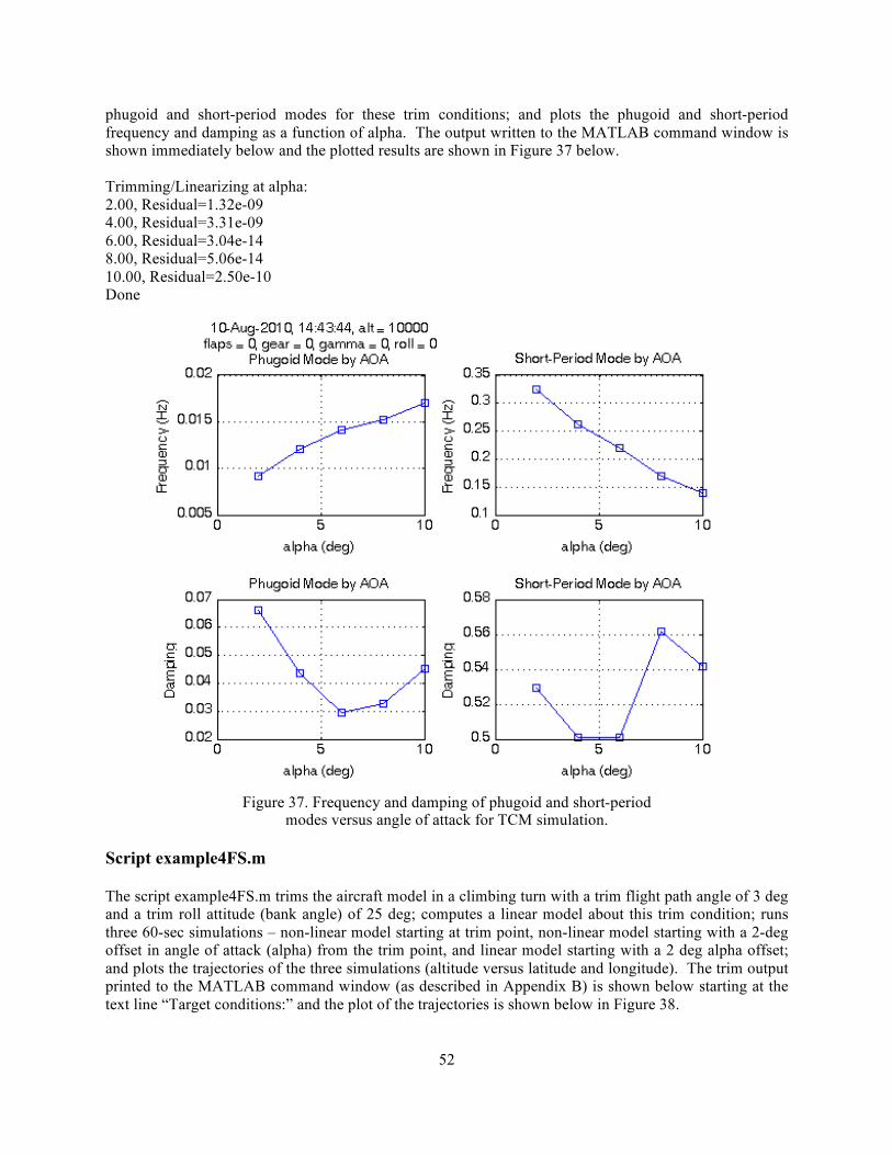
52

phugoid and short-period modes for these trim conditions; and plots the phugoid and short-period frequency and damping as a function of alpha. The output written to the MATLAB command window is shown immediately below and the plotted results are shown in Figure 37 below. Trimming/Linearizing at alpha: 2.00, Residual=1.32e-09 4.00, Residual=3.31e-09 6.00, Residual=3.04e-14 8.00, Residual=5.06e-14 10.00, Residual=2.50e-10 Done

Figure 37. Frequency and damping of phugoid and short-period

modes versus angle of attack for TCM simulation.

Script example4FS.m

The script example4FS.m trims the aircraft model in a climbing turn with a trim flight path angle of 3 deg and a trim roll attitude (bank angle) of 25 deg; computes a linear model about this trim condition; runs three 60-sec simulations – non-linear model starting at trim point, non-linear model starting with a 2-deg offset in angle of attack (alpha) from the trim point, and linear model starting with a 2 deg alpha offset; and plots the trajectories of the three simulations (altitude versus latitude and longitude). The trim output printed to the MATLAB command window (as described in Appendix B) is shown below starting at the text line “Target conditions:” and the plot of the trajectories is shown below in Figure 38.

53

Optimizing using simulink function nlconst... Done Target conditions: cas: 200.00 gamma: 3.00 roll: 25.00 beta: 0.00 pitchrate: 0.00 rollrate: 0.00 Trim Errors: beta: -3.13e-13 cas: -7.43e-28 gamma: 4.44e-16 pitchrate: 0.00e+00 roll: 4.97e-17 rollrate: 0.00e+00 Trim conditions (Err=6.054e-11) gamma: 3.00 tas: 231.56 alt: 10000.00 mach: 0.3627 cas: 200.00 alpha: 3.94 beta: -0.00 pdeg: -0.25 qdeg: 0.92 rdeg: 1.97 roll: 25.00 pitch: 6.57 yaw: 90.00 gndtrack:88.33 rollrate: 0.00 pitchrate: 0.00 yawrate: 2.19 elevator: 0.00 stabilizer: 0.30 ailerons: 0.40 rudder:-0.70 throttle: 48.01 speedbrake: 0.00 flaps: 5.00 geardown: 0.00 d/dt(u,v,w,p,q,r) [6.05e-11 8.88e-15 -4.71e-12 -7.59e-15 4.65e-13 2.64e-15] d/dt(phi,theta,psi) [8.67e-19 0.00e+00 3.81e-02] Linearizing... Done Simulating... Done, Running at 4.35 times real-time Simulating... Done, Running at 4.27 times real-time

Figure 38. Climbing turn simulated trajectories for TCM simulation.

54

References

1. Publicly available software release package of Langley Research Center, “Flight Dynamics Simulation of a Generic Transport Model”, Case No: LAR-17625-1 available by request to Langly Research Center’s Software Releasing Authority.

2. Kaneshige, John T., Cox, David E., Cunningham, Kevin, Shah, Gautam H., Nguyen, Nhan, Totah, Joe, Krishnakumar, Kalmanje, Panda, Ramesh, and Steglinski, Mietek: non-published report within the Integrated Resilient Aircraft Controls element of the NASA Aviation Safety Program, electronic PDF file titled Full Scale GTM.pdf, March 12, 2008.

3. Glenn Research Center, Air Viscosity – Sutherland’s Formula, www.grc.nasa.gov/WWW/BGH/viscosity.html accessed April, 2008.

4. William H. Rae Jr. and Alan Pope, Low-Speed Wind Tunnel Testing, 2nd Ed., Wiley-Interscience, 1984.

5. Standford University, Maximum Lift Prediction -- Specific Conceptual Design Method, http://adg.stanford.edu/aa241/highlift/clmaxest.html accessed April 2008.

6. May, Ryan D., Csank, Jeffrey, Lavelle, T. M., Litt, Jonathan S., and Guo, Ten-Huei, A High-Fidelity Simulation of a Generic Commercial Aircraft Engine and Controller, AIAA-2010-6630, 46th AIAA/ASME/SAE/ASEE Joint Propulsion Conference and Exhibit, Nashville, TN, July 25-28, 2010, also NASA/TM-2010-216810, October 2010.

7. Hanke, Rodney C. and Nordwall, Donald R.: The Simulation of a Jumbo Jet Transport Aircraft, Vol. II: Modeling Data, Boeing Document D6-30643-VOL-2/NASA CR-114494, Sept 1970.

8. NTSB Aircraft Accident Report PB99-910401, USAIR flight 427, Uncontrolled Descent and Collision with Terrain, September 8, 1994.

9. Wolowicz, Chester H., Bowman, James S. Jr., and Gilbert, William P.: Similitude Requirements and Scaling Relationships as Applied to Model Testing, NASA TN 1435, August 1979.

REPORT DOCUMENTATION PAGEForm Approved

OMB No. 0704-0188

2. REPORT TYPE

Technical Memorandum 4. TITLE AND SUBTITLE

Development of the Transport Class Model (TCM) Aircraft Simulation From a Sub-Scale Generic Transport Model (GTM) Simulation

5a. CONTRACT NUMBER

6. AUTHOR(S)

Hueschen, Richard M.

7. PERFORMING ORGANIZATION NAME(S) AND ADDRESS(ES)

NASA Langley Research CenterHampton, VA 23681-2199

9. SPONSORING/MONITORING AGENCY NAME(S) AND ADDRESS(ES)

National Aeronautics and Space AdministrationWashington, DC 20546-0001

8. PERFORMING ORGANIZATION REPORT NUMBER

L-20050

10. SPONSOR/MONITOR'S ACRONYM(S)

NASA

13. SUPPLEMENTARY NOTES

12. DISTRIBUTION/AVAILABILITY STATEMENTUnclassified UnlimitedSubject Category 01 Availability: NASA CASI (443) 757-5802

19a. NAME OF RESPONSIBLE PERSON

STI Help Desk (email: help@sti.nasa.gov)

14. ABSTRACT

A six degree-of-freedom, flat-earth dynamics, non-linear, and non-proprietary aircraft simulation was developed that is representative of a generic mid-sized twin-jet transport aircraft. The simulation was developed from a non-proprietary, publicly available, subscale twin-jet transport aircraft simulation using scaling relationships and a modified aerodynamic database. The simulation has an extended aerodynamics database with aero data outside the normal transport-operating envelope (large angle-of-attack and sideslip values). The simulation has representative transport aircraft surface actuator models with variable rate-limits and generally fixed position limits. The simulation contains a generic 40,000 lb sea level thrust engine model. The engine model is a first order dynamic model with a variable time constant that changes according to simulation conditions. The simulation provides a means for interfacing a flight control system to use the simulation sensor variables and to command the surface actuators and throttle position of the engine model.

15. SUBJECT TERMS

transport aircraft simulation; extended aerodynamic database; flight control system interface; scaled aircraft simulation; high angle-of-attack; large sideslip aerodynamic database

18. NUMBER OF PAGES

61

19b. TELEPHONE NUMBER (Include area code)

(443) 757-5802

a. REPORT

U

c. THIS PAGE

U

b. ABSTRACT

U

17. LIMITATION OF ABSTRACT

UU

Prescribed by ANSI Std. Z39.18Standard Form 298 (Rev. 8-98)

3. DATES COVERED (From - To)

5b. GRANT NUMBER

5c. PROGRAM ELEMENT NUMBER

5d. PROJECT NUMBER

5e. TASK NUMBER

5f. WORK UNIT NUMBER

432938.11.01.07.43.16.01

11. SPONSOR/MONITOR'S REPORT NUMBER(S)

NASA/TM-2011-217169

16. SECURITY CLASSIFICATION OF:

The public reporting burden for this collection of information is estimated to average 1 hour per response, including the time for reviewing instructions, searching existing data sources, gathering and maintaining the data needed, and completing and reviewing the collection of information. Send comments regarding this burden estimate or any other aspect of this collection of information, including suggestions for reducing this burden, to Department of Defense, Washington Headquarters Services, Directorate for Information Operations and Reports (0704-0188), 1215 Jefferson Davis Highway, Suite 1204, Arlington, VA 22202-4302. Respondents should be aware that notwithstanding any other provision of law, no person shall be subject to any penalty for failing to comply with a collection of information if it does not display a currently valid OMB control number.PLEASE DO NOT RETURN YOUR FORM TO THE ABOVE ADDRESS.

1. REPORT DATE (DD-MM-YYYY)

08 - 201101-