Embed Size (px)
Citation preview
Perception & Psychophysics1988. 43. 241-277
Neural dynamics of I-D and 2-D brightnessperception: A unified model of classical
and recent phenomena
STEPHEN GROSSBERGBoston University, Boston, Massachusetts
and
DEJAN TODOROVICBoston University, Boston, Massachusetts
and Univerzitet u Beogradu, Belgrade, Yugoslavia
Computer simulations of a neural network model of I-D and 2-D brightness phenomena arepresented. The simulations indicate how configural image properties trigger interactions amongspatially organized contrastive, boundary segmentation, and filling-in processes to generate emergent percepts. They provide the first unified mechanistic explanation of this set of phenomena,a number of which have received no previous mechanistic explanation. Network interactions between a Boundary Contour (BC) System and a Feature Contour (FC) System comprise the model.The BC System consists of a hierarchy of contrast-sensitive and orientationally tuned interactions, leading to a boundary segmentation. On and off geniculate cells and simple and complexcortical cells are modeled. Output signals from the BC System segmentation generate compartmental boundaries within the FC System. Contrast-sensitive inputs to the FC System generatea lateral filling-in of activation within FC System compartments. The filling-in process is defined by a nonlinear diffusion mechanism. Simulated phenomena include network responses tostimulus distributions that involve combinations of luminance steps, gradients, cusps, and cornersof various sizes. These images include impossible staircases, bull's-eyes, nested combinations ofluminance profiles, and images viewed under nonuniform illumination conditions. Simulatedphenomena include variants of brightness constancy, brightness contrast, brightness assimilation, the Craik-O'Brien-Cornsweet effect, the Koffka-Benussi ring, the Kanizsa-Minguzzianomalous brightness differentiation, the Hermann grid, and a Land Mondrian viewed underconstant and gradient illumination that cannot be explained by retinex theory.
PART 1INTRODUCTION: INTERACTIONS BETWEEN
FORM AND APPEARANCE
The sensitivity to ambient differences in light energyis the most basic discriminative ability of visual systems.The distribution of light energy reaching an animal's eyesis often characterized by regions of slow or zero gradientsbordered by abrupt changes such as edges or contours.Correspondingly, one important tradition of psychophysical investigation has intensively studied the perceptualproperties of juxtaposed homogeneous regions, leading
S.G. 's work was supported in part by the Air Force Office of Scientific Research (AFOSR F49620-87-C-0018 and AFOSR F49620-86-C0037) and the Anny Research Office (ARO DAAG-29-85-K-00(5).D.T. 's work was supported in part by the Anny Research Office (ARODAAG-29-85-K-0095). The authors thank Cynthia Suchta and CarolYanakakis for their valuable assistance in the preparation of themanuscript and illustrations. S.G. 's mailing address is Center for Adaptive Systems, Boston University, III Cummington Street, Boston, MA02215. D.T. 's mailing address is Filozofski Fakultet, Cika Ljubina 1820, 11000 Belgrade, Yugoslavia.
to such classical contributions as Weber's ratio and Fechner's law (Fechner, 1889), Metzger's Ganzfeld (Metzger, 1930), and the analysis of brightness constancy andcontrast (Hess & Pretori, 1894; Katz, 1935). A parallelline of psychophysical investigation has emphasized theprocessing of luminancediscontinuities, notably edges andtextures (Beck, 1966a, 1966b; Julesz, 1971; Ratliff,1965).
Each type of investigation has provided essential dataand concepts about visual perception, but, taken in isolation, each is nonetheless inherently incomplete. For example, the output of an edge-processing model producesonly an outline of its visual environment and provides insufficient information about either the form or the appearance of the structures within the outline.
The nature of the incompleteness of vision concepts andmodels that focus on only one type of process at the expense of the other can be understood from two differentperspectives. On the one hand, there exist large data baseswhich support the hypothesis that the processes that control the perception of form and appearance strongly interact before generating a final percept. Data concerning
241 Copyright 1988 Psychonomic Society, Inc.
242 GROSSBERG AND TODOROVIC
Figure 1. The Kanizsa-Minguzzi anomalous brightness differentiation. The bright annulus is divided into two unequal segments.The smaller segment looks slightly brighter.
one-dimensional (1-0) and 2-D brightness perception provide a particularly rich and constraining set of phenomenaof this type. A number of key phenomena from this database are given a unified explanation herein. In our modelthese brightness phenomena are generated as emergentproperties of a neural network theory of preattentive visualperception (Cohen & Grossberg, 1984; Grossberg, 1987a,1987b; Grossberg & Mingolla, 1985a, 1985b, 1987,1988).
The anomalous brightness differentiation (Kanizsa &Minguzzi, 1986) that is induced by the image shown inFigure 1 is one of the many brightness phenomena thatcan be explained by this theory. As Kanizsa and Minguzzi(1986) have noted, "this unexpected effect is not easilyexplained. In fact, it cannot be accounted for by any simple physiological mechanism such as lateral inhibition orfrequency filtering, Furthermore, it does not seem obvious to invoke organizational factors, like figural belongingness of figure-ground articulation" (p. 223). We agreewith these authors, but also show that this brightnessphenomenon can be explained by the same theory that weuse to explain many other brightness phenomena.
The properties of this theory clarify a deeper sense inwhich models that consider only form or appearance areincomplete. The perceptual theory that we apply suggeststhat each of the neural systems that process form or appearance compensates for limitations of the other systemswith which it interacts. In other words, complete articulation of the processing rules for either system requiresan analysis of the processing rules of the other systemand of how the systems offset each other's complementary inadequacies through their interactions. Such an analysis has led to the identification of several new uncertaintyprinciples which these systems overcome through paralleland hierarchical interactions (Grossberg, 1987a, 1987b).
The theory suggests that two parallel contour-sensitiveprocesses interact to generate a percept of brightness. TheBoundary Contour (BC) System, defined by a networkhierarchy of oriented interactions, synthesizes an emergent binocular boundary segmentation from combinationsof oriented and unoriented scenic elements. The FeatureContour (Fe) System triggers a diffusive filling-in offeatural quality within perceptual domains whose bound-
aries are determined by output signals from the BC System. Neurophysiological and anatomical data from lateralgeniculate nucleus and visual cortex which have been analyzed and predicted by the theory are summarized inGrossberg (l987a, 1987b).
Herein we use a simplified version of the model to explain brightness data. The simplified model does not include BC System and FC System mechanisms of emergent segmentation, multiple scale filtering, binocularinteractions, and double-opponent processing. We focuson that large domain of brightness data whose qualitativeproperties can be explained by a single-scale, monocularversion of the model. Our computer simulations of 1-Dphenomena use a single set of numerical parameters, asdo our simulations of 2-D brightness phenomena. We alsoshow how parameter changes influence quantitative details of the simulation results. Since many visual imagesactivate multiple spatial scales, binocular interactions, andemergent segmentations, our goal herein is to provide thetype of quantitative understanding of model mechanismsthat can achieve a unified qualitative explanation ofdifficult brightness data. The explanations of brightnessphenomena within this reduced model are easily seen tobe valid within the full theory, and to provide necessaryinformation for future studies of quantitative matches between simulations and data in a multiple-scale, binocularsetting.
The present article is organized as follows. In Part 2we describe the neural network model that we use to simulate brightness phenomena. This model generalizes to twodimensions the types of processes that Cohen and Grossberg (1984) used to simulate I-D brightness phenomena.This generalization conjoins processing concepts andmechanisms from Cohen and Grossberg (1984) and thosefrom Grossberg and Mingolla (l985b, 1987). Part 3 defines and illustrates model properties through computersimulations of the model's reactions to a particular 2-Dluminance distribution called the yin-yang square. Thenext two sections provide a unified account, through computer simulations, of several classical and recent varietiesof brightness phenomena. Part 4 contains the I-D simulations and Part 5 contains the 2-D simulations. Part 6 discusses how the model's concepts and mechanisms arerelated to other concepts and mechanisms of the theorywhich have been developed to analyze different data bases.
PART 2THE MODEL: A HIERARCHY OF SPATIALLY
ORGANIZED NETWORK INTERACTIONS
Figure 2 provides an overview of the neural networkmodel that we have analyzed. The model has six levelsdepicted as thick-bordered rectangles numbered from 1to 6. Levels 1 and 2 are preprocessing levels prior to theBC and FC Systems. Output signals from Level 2 generate inputs to both of these systems. Levels 3-5 are processing stages within the BC System. Level 6, which models
NEURAL DYNAMICS OF I-D AND 2-D BRIGHTNESS PERCEPTION 243
1
Figure 2. Overview of the model. The thick-bordered rectanglesnumbered from 1 to 6 correspond to the levels of the system. Thesymbols inside the rectangles are graphical mnemonics for the typesof computational units residing at the corresponding model level.The arrows depict tbe interconnections between the levels. The thinbordered rectangles coded by letters A through E represent the typeof processing between pairs of levels. Inset F illustrates how the activity at Level 6 is modulated by outputs from Level 2 and Level S.See text for additional details.
the FC System, receives inputs from both Level 2 andLevelS.
Each level contains a different type of neural network.The type of network is indicated by the symbol inside therectangle. The symbols provide graphical mnemonics forthe processing characteristicsat a given level, and are usedin the figures that present the computer simulations of the2-D implementation of the model. The arrows connecting the rectangles depict the flow of processing betweenthe levels. The type of signal processing between different levels is indicated inside thin-bordered insets attachedby dotted lines to appropriate arrows, and coded by letters A through E. The sketch inside the inset coded Fdepicts the complex interactions between Levels 2,5, and6. The properties of different levels and transformationswill be discussed in detail in the following pages. To explain the working of the system, we repeatedly refer toFigure 2, and present a number of computer simulationsof network dynamics. The mathematical equations of themodel are described in the Appendix.
Levell: The Stimulus DistributionThe first level of the model consists of a set of units
that sample the luminance distribution. In the I-D version of the model, the units are arranged on a line; in the2-D version, they form a square grid.
Level 2: Circular Concentric On and Off Units(LGN Cells)
Level 2 of the network models cells with the type ofcircular concentric receptive fields found at early levelsof the visual system, such as ganglion retinal cells orlateral geniculate cells. These cells come in two varieties:the on-center-off-surround cells, or on-cells, and the offcenter-on-surround cells, or off-cells. In Figure 2, theon-cells are symbolized with a white center and a blackannulus, and the off-cells with a black center and a whiteannulus. The mathematical specification of the receptivefield (see the Appendix) uses feedforward shunting equations (Grossberg, 1983) because of their sensitivity to input reflectances. Thus, the model utilizes the simplestphysiological mechanismthat discounts the illuminantandis sufficient to explain key properties of the targetedbrightness percepts.
The 1-D cross-sections of these receptive fields arepresented in insets A and B in Figure 2. In two dimensions, these profiles have the shape of sombreros for onunits and inverted sombreros for off-units. The activitylevel of such cells correlates with the size of the centersurround luminance contrast. More luminance in thecenter than in the surround induces increased activity inon-cells and decreased activity in off-cells. Inverse luminance conditionsresult in inverse activation levels. Dueto the shunting interaction, the cells are sensitive to relative contrast in a manner approximating a Weber law(Grossberg, 1983). In addition, the cells are tuned to display nonnegligible activity levels even for homogeneousstimulation, as do retinal ganglion cells (Enroth-Cugell& Robson, 1984). This property enables such a cell togenerate output signals that are sensitive to both excitatory and inhibitory inputs.
Level 3: Oriented Direction-of-Contrast-SensitiveUnits (Simple Cells)
Level 3 consists of cell units that share properties withcortical simple cells. The symbol for these units inFigure 2 expresses their sensitivity to luminance contrastof a given orientation and given direction of contrast. Inset C depicts the I-D cross-section of the receptive fieldof such units, taken with respect to the network of on-eells.
In our 2-D simulations, the function we used to generate this receptive field profile was the difference of twoidentical bivariate Gaussians whose centers were shiftedwith respect to each other (see the Appendix). A similarformalization was used by Heggelund (l981a, 1985). Asyet, neither anatomical nor physiological studies have unequivocally demonstrated the manner in which orienta-
F
@ ~
01.01.0t t· t000
5
6
2
[Q].-~6 .-4.. t~-1 CD001,-------, 8·i(}!z>
,Ie t--~
~~~ITJ-~2t-rn 3
B @] A
244 GROSSBERG AND TODOROVIC
tiona! sensitivity arises in cortical cells (Braitenberg &Braitenberg, 1979; Nielsen, 1985; Sillito, 1984). Our ambition was not to resolve this issue, but to find a simple,yet acceptable, arrangement that would realize the desiredfunctional properties. In our current implementation,Level 3 units are activated by Level 2 on-units.
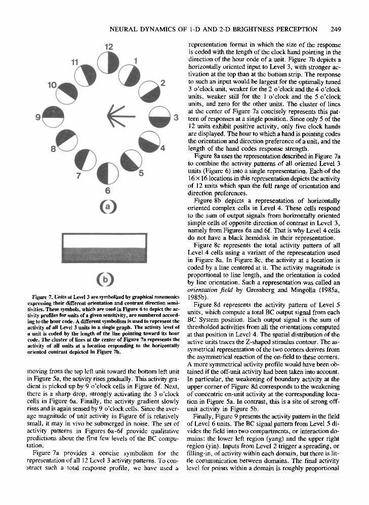
In order to represent a number of different orientationsensitivities, Level 3 consists of 12 different cell types,each sensitive to a different orientation and direction ofcontrast. A convenient "hour code" was used to denotethese units. For example, a cell tuned to detect verticalleft-to-right light-dark edges is denoted a "12 o'clockunit," whereas a cell with the same axis orientation butreversed contrast preference is a "6 o'clock unit" (seeFigure 7). In the 1-D implementation, only two directionswere used.
Level 4: Oriented Direction-of-Contrast-InsensitiveUnits (Complex Cells)
Level 3 units are sensitive to oriented contrasts in aspecific direction-of-contrast, as are cortical simple cells.However, complex cell units sensitive to contrasts ofspecific orientation regardless of contrast polarity are alsowell known to occur in striate cortical area 17 of monkeys (DeValois, Albrecht, & Thorell, 1982; Gouras &Kruger, 1979; Hubel & Wiesel, 1968; Schiller, Finlay,& Volman, 1976; Tanaka, Lee, & Creutzfeldt, 1983) andcats (Heggelund, 1981b; Hubel & Wiesel, 1962; Spitzer& Hochstein, 1985). See Grossberg (1987a) for a reviewof relevant data and related models.
Units fulfIlling the above criteria populate Level 4 ofthe network. Inset D in Figure 2 depicts the constructionof Level 4 cells out of Level 3 cells. The mathematicalspecification is similar to the one used by Grossberg andMingolla (1985a, 1985b) and Spitzer and Hochstein(1985). The symbol of Level 4 units expresses their sensitivity to oriented contrasts of either direction. EachLevel 4 unit at a particular location is excited by 2 Level 3units at the corresponding location having the same axisof orientation but opposite direction preference. For example, a 3 o'clock unit and a 9 o'clock unit in Level 3generate a horizontal contrast detector in Level 4. Thus,the 12 Level 3 networks give rise to 6 Level 4 networks.Interestingly, several physiological studies have found thatthe simple cells outnumber the complex cells in a ratioof approximately 2 to 1, and that complex cells havehigher spontaneous activity levels than simple cells (Kato,Bishop, & Orban, 1978). Both of these properties are consistent with the proposed circuitry.
Level 5: Boundary Contour UnitsIn the simulations presented in this paper, we have used
a simplified version of the BC System. The final outputof this system is located at Level 5 of the model. A unitat a given Level 5 location can be excited by any Level 4unit located at the position corresponding to the position
of the Level 5 unit. A Level 4 unit excites a Level 5 unitonly if its own activity exceeds a threshold value. Thepooling of signals sensitive to different orientations issketched in inset E and expressed in the symbol forLevel 5 in Figure 2. This pooling may, in principle, occur entirely in convergent output pathways from the BCSystem to the FC System, rather than at a separate levelof cells within the BC System.
Level 6: Diffusive Filling-In Within a Cell SyncytiumNetwork activity at Level 6 of our model corresponds
to the brightness percept. Level 6 is part of the FC System, which is composed of a syncytium of cells. A syncytium of cells is a regular array of intimately connectedcells such that contiguous cells can easily pass signals between each other's compartment membranes, possible viagap junctions (Piccolino, Neyton, & Gerschenfeld, 1984).Due to the syncytial coupling of each cell with its neighbors, the activity can rapidly spread to neighboring cells,then to neighbors of the neighbors, and so on.
Because the spreading, or filling-in, of activation occurs via a process of diffusion, it tends to average the activation that is triggered by a FC input from Level 2 acrossthe Level 6 cells that receive this spreading activity. Thisaveraged activity spreads across the syncytium with aspace constant that depends upon the electrical activitiesof both the cell interiors and their membranes. The electrical properties of the cell membranes can be altered byBC signals in the following way. A BC signal is assumedto decrease the diffusion constant of its target cell membranes within the cell syncytium. It does so by acting asan inhibitory gating signal that causes an increase in cellmembrane resistance. A BC signal hereby creates a barrier to the filling-in process at its target cells.
The inset labeled F in Figure 2 summarizes the threefactors that influence the magnitude of activity of unitsat Level 6. First, each unit receives bottom-up input fromLevel 2, the field of concentric on-cells. Second, thereare lateral connections between neighboring units atLevel 6 that define the syncytium, which enables withinnetwork spread of activation, or filling-in. Third, thislateral spread is modulated by inhibition from Level 5 inthe form of BC signals capable of decreasing the magnitude of mutual influence between neighboring Level 6units. The net effect of these interactions is that the FCsignals generated by the concentric on-cells are diffusedand averaged within boundaries generated by BC signals.
The idea of a filling-in process has been invoked invarous forms by several authors in discussions of different brightness phenomena (Davidson & Whiteside, 1971;Fry, 1948; Gerrits & Vendrik, 1970; Hamada, 1984;Walls, 1954). In the present model, this notion is fullyformalized, related to a possible neurophysiological foundation, tied in with other mechanisms as a part of a moregeneral vision theory, and applied in a systematic wayto a variety of brightness phenomena.
NEURAL DYNAMICS OF I-D AND 2-D BRIGHTNESS PERCEPTION 245
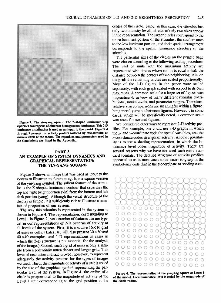
Figure 3. The yin-yang square. The Z-shaped luminance stepseparates two regions of different homogeneousluminance. This 2-Dluminance distribution is used as an input to the model. Figures 4through 9 present the activity profiles induced hy this stimulus atvarious levels of the model. The equations and parameters used inthe simulations are listed in the Appendix.
PART 3AN EXAMPLE OF SYSTEM DYNAMICS AND
GRAPIDCAL REPRESENTATION:THE YIN-YANG SQUARE
Figure 3 shows an image that was used as input to thesystem to illustrate its functioning. It is a square versionof the yin-yang symbol. The salient feature of the stimulus is the Z-shaped luminance contour that separates thetop and right bright portion (yin) from the bottom and leftdark portion (yang). Although the visual structure of thedisplay is simple, it is sufficiently rich to illustrate a number of properties of our system.
The way this stimulus is represented in the system isshown in Figure 4. This representation, corresponding toLevel 1 in Figure 2, has a number of features that are typical in our representations of 2-D patterns of activity atall levels of the system. First, it is a square 16X 16 gridof units or cells. (Later, we will also present 30x30 and40x40 examples, and I-D representations in cases inwhich the 2-D structure is not essential for the analysisof the image.) Second, such a grid ofunits is only a sample from a potentially much denser and larger grid. Thislevel of resolution and size proved, however, to representadequately the activity patterns for the types of imageswe used. Third, the magnitudeof activity of a unit is codedby the size of the graphical symbol representing the particular level of the system. In Figure 4, the radius of acircle is proportional to the magnitude of activity of theLevel 1 unit corresponding to the grid position at the
center of the circle. Since, in this case, the stimulus hasonly two intensity levels, circles of only two sizes appearin the representation. The larger circles correspond to themore luminant portion of the stimulus, the smaller onesto the less lurninant portion, and their spatial arrangementcorresponds to the spatial luminance structure of thestimulus.
The particular sizes of the circles on the printed pagewere chosen according to the following scaling procedure:The unit or units with the maximum activity arerepresented with circles whose radius is equal to half thedistance between the centers of two neighboring units onthe grid; the remaining circles are scaled proportionally.Most of the 2-D figures in the paper were scaledseparately, with each graph scaled with respect to its ownmaximum. A common scale for a large set of figures wasimpracticable in view of many different stimulus distributions, model levels, and parameter ranges. Therefore,relative size comparisons are meaningful within a figure,but generally are not between figures. However, in somecases, which will be specifically noted, a common scalewas used for several figures.
We considered other ways to represent 2-D activity profiles. For example, one could use 3-D graphs in whichthe x- and y-eoordinate code the spatial variables, and thez-coordinate codes strength of activity. Another possibility is to use a shading representation, in which the luminance level codes magnitude of activity. There areseveral reasons why we have not used such more standard formats. The detailed structure of activity profilesappeared to us in most cases to be easier to grasp in thesymbol-size code than in the z-eoordinate or shadingcode.
0000000000000000
'-..-" "-"" "-
0000000000000000000000000000000000000000000000000000000000000000000000000000000000000000000000000000000000000000
Figure 4. The representation of the yin-yang square at Level 1of the model. Local luminance level is coded by the magnitude ofthe circle radius.
246 GROSSBERG AND TODOROVIC
The hidden-line-removal technique, used in some versionsof the first code, unfortunately also hides some aspectsof the profile structure. A shading representation seemedto us particularly awkward, since our purpose was to studythe more subtle and illusory aspects of brightness perception. On the other hand, since a symbol has other features in addition to size, these other features can be usedto code other aspects of activity profiles. As illustratedherein, the use of different mnemonic symbols for different levels of the system enhances the clarity of presentation of its structure and function. The advantages of asymbol-size representation become apparent in therepresentation of the Level 2 response to the yin-yangsquare.
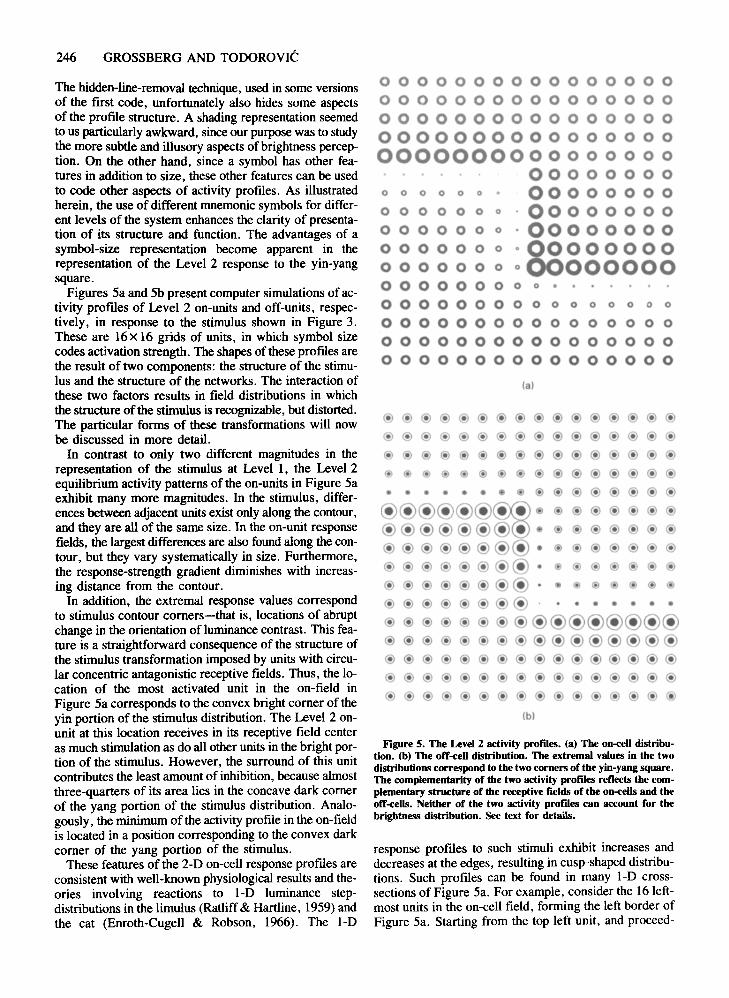
Figures 5a and 5b present computer simulations of activity profiles of Level 2 on-units and off-units, respectively, in response to the stimulus shown in Figure 3.These are 16x 16 grids of units, in which symbol sizecodes activation strength. The shapes of these profiles arethe result of two components: the structure of the stimulus and the structure of the networks. The interaction ofthese two factors results in field distributions in whichthe structure of the stimulus is recognizable, but distorted.The particular forms of these transformations will nowbe discussed in more detail.
In contrast to only two different magnitudes in therepresentation of the stimulus at Levell, the Level 2equilibrium activity patterns of the on-units in Figure 5aexhibit many more magnitudes. In the stimulus, differences between adjacent units exist only along the contour,and they are all of the same size. In the on-unit responsefields, the largest differences are also found along the contour, but they vary systematically in size. Furthermore,the response-strength gradient diminishes with increasing distance from the contour.
In addition, the extremal response values correspondto stimulus contour corners-that is, locations of abruptchange in the orientation of luminance contrast. This feature is a straightforward consequence of the structure ofthe stimulus transformation imposed by units with circular concentric antagonistic receptive fields. Thus, the location of the most activated unit in the on-field inFigure 5a corresponds to the convex bright corner of theyin portion of the stimulus distribution. The Level 2 onunit at this location receives in its receptive field centeras much stimulation as do all other units in the bright portion of the stimulus. However, the surround of this unitcontributes the least amount of inhibition, because almostthree-quarters of its area lies in the concave dark cornerof the yang portion of the stimulus distribution. Analogously, the minimum of the activity profile in the on-fieldis located in a position corresponding to the convex darkcorner of the yang portion of the stimulus.
These features of the 2-D on-cell response profiles areconsistent with well-known physiological results and theories involving reactions to I-D luminance stepdistributions in the limulus (Ratliff & Hartline, 1959) andthe cat (Enroth-Cugell & Robson, 1966). The I-D
00000000000000000000000000000000000000000000000000000000000000000000000000000000
00000000000000. OOOOOOO~
0000000 00000000o 0 0 0 0 0 0 00000 0 0 0000000 0°00000000
0000000 00000000000000000 0.000 0 000 0 0 0 0 0 0 0 0 0
000000000000000000000000000000000000000000000000
(a)
@ @ @ @ @ @ @ @ @ @ @ @ @ @ @ @@ @ @ @ @ @ @ @ @ @ @ @ @ @ @ @@ @ @ @ @ @ @ @ @ @ @ @ @ @ @ @
@ @ @ @ @ @ @ @ @ @ @ @ @ @ @ @.. .. .. .. • .. @ @ @ @ @ @ @ @ @ @
@@@@@@~@ @ @ @ @ @ @ @
@@@@@@@e@ @ @ @ @ @ @ @@@@ @ @@@@. @ @ @ @ @ @ @
@@@ @ @@@@- @ @ @ @ @ @ @
@@@ @ @@@@. <§l @ @ @ @ @ @
@ @ @ @ @@@@ - II II II II •@@@ @ @@@@@@@@@@@@@ @ @ @ @@@@@@@@@@@@@ @ @ @ @@@@@@@@@@@@@@@ @ @@@@@@@@@@@@@@@ @ @@@@@@@@@@@@
(bl
Figure 5. The Level 2 activity profiles. (a) The on-eell distribution. (b) The off-eell distribution. The extremal values in the twodistributions correspond to the two corners of the yin-yang square.The complementarity of the two activity profiles reflects the complementary structure of the receptive fields of the on-eells and theoff-eells. Neitber of the two activity profiles can account for thebrightness distribution. See text for details.
response profiles to such stimuli exhibit increases anddecreases at the edges, resulting in cusp-shaped distributions. Such profiles can be found in many I-D crosssections of Figure 5a. For example, consider the 16 leftmost units in the on-cell field, forming the left border ofFigure Sa. Starting from the top left unit, and proceed-
NEURAL DYNAMICS OF 1-D AND 2-D BRIGHTNESS PERCEPTION 247
ing toward the bottom left unit, the activity level increasestoward the luminance edge, drops abruptly, and returnsgradually to a medium level. It is widely accepted thatthese overshoots and undershoots in physiological activitycontribute to the phenomenon of Mach bands (Ratliff,1965).
The corner-related extrema in the Level 2 distributionprofiles may contribute to the enhanced brightnessphenomena involving nested sets of corners that were analyzed by Hurvich (1981), who discovered them in paintings by Vasarely. Analogous effects were described byTodorovic (1983) in some related visual situations. Inanalogy to Mach bands, they might be called "Machcorners." A corresponding physiological study has, to ourknowledge, not been performed.
A comparison of the on-unit activity pattern in Figure 5awith the off-unit activity pattern in Figure 5b shows a symmetry, or duality, due to the complementary structure ofthe receptive fields of on-units and off-units. For example, the locus of minimum activity in Figure 5a corresponds to the locus of maximum activity in Figure 5b,and vice versa. The regions of activity overshoots and undershoots along stimulus contours have also exchangedlocations. More generally, for any two units (and, in particular, for any two adjacent units), the following observation holds: If, in Figure 5a, the activity of the first unitis larger than the activity of the second one, then, for thetwo corresponding units in Figure 5b, the activity of thefirst unit will be smaller than the activity of the secondone, and vice versa.
The final point with respect to the shapes of Level 2profiles concerns the regions located at some distancefrom the Z-shaped contour. For example, consider thebottom left and the top right unit, whose locations are mostremoved from the contour region. Their activity level isapproximately the same, both within the on-unit field andwithin the off-unit field. This equality in activity level contrasts with the appearance of the corresponding image portions (Figure 3): the lower left region of the image appears darker than the upper right region. This aspect ofthe brightness profile cannot be accounted for by the activity profile of cells with concentric antagonistic receptive fields, which are insensitive to differences of the absolute level of homogeneous stimulation. In the model,the brightness of Figure 3 is accounted for by the Level 6distribution.
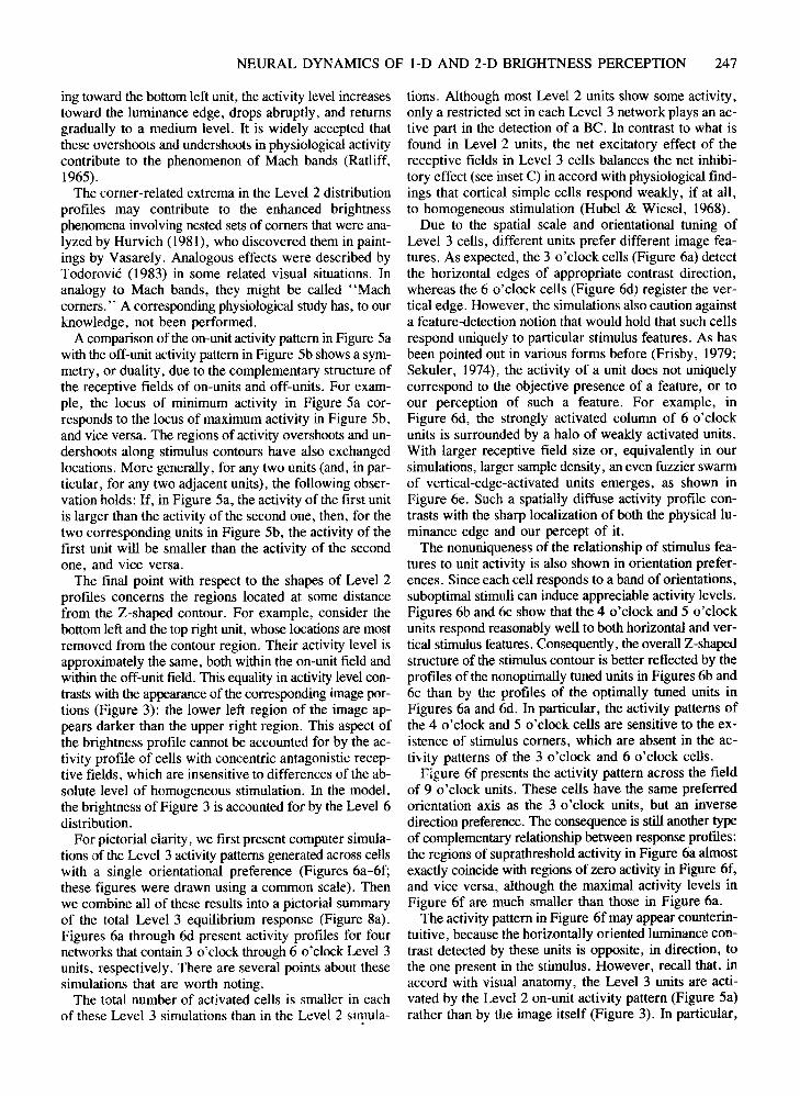
For pictorial clarity, we first present computer simulations of the Level 3 activity patterns generated across cellswith a single orientational preference (Figures 6a-6f;these figures were drawn using a common scale). Thenwe combine all of these results into a pictorial summaryof the total Level 3 equilibrium response (Figure 8a).Figures 6a through 6d present activity profiles for fournetworks that contain 3 o'clock through 6 o'clock Level 3units, respectively. There are several points about thesesimulations that are worth noting.
The total number of activated cells is smaller in eachof these Level 3 simulations than in the Level 2 sirnula-
tions. Although most Level 2 units show some activity,only a restricted set in each Level 3 network plays an active part in the detection of a Be. In contrast to what isfound in Level 2 units, the net excitatory effect of thereceptive fields in Level 3 cells balances the net inhibitory effect (see inset C) in accord with physiological findings that cortical simple cells respond weakly, if at all,to homogeneous stimulation (Hubel & Wiesel, 1968).
Due to the spatial scale and orientational tuning ofLevel 3 cells, different units prefer different image features. As expected, the 3 o'clock cells (Figure 6a) detectthe horizontal edges of appropriate contrast direction,whereas the 6 o'clock cells (Figure 6d) register the vertical edge. However, the simulations also caution againsta feature-detection notion that would hold that such cellsrespond uniquely to particular stimulus features. As hasbeen pointed out in various forms before (Frisby, 1979;Sekuler, 1974), the activity of a unit does not uniquelycorrespond to the objective presence of a feature, or toour perception of such a feature. For example, inFigure 6d, the strongly activated column of 6 o'clockunits is surrounded by a halo of weakly activated units.With larger receptive field size or, equivalently in oursimulations, larger sample density, an even fuzzier swarmof vertical-edge-activated units emerges, as shown inFigure 6e. Such a spatially diffuse activity profile contrasts with the sharp localization of both the physicalluminance edge and our percept of it.
The nonuniqueness of the relationship of stimulus features to unit activity is also shown in orientation preferences. Since each cell responds to a band of orientations,suboptimal stimuli can induce appreciable activity levels.Figures 6b and 6c show that the 4 o'clock and 5 o'clockunits respond reasonably well to both horizontal and vertical stimulus features. Consequently, the overall Z-shapedstructure of the stimulus contour is better reflected by theprofiles of the nonoptimally tuned units in Figures 6b and6c than by the profiles of the optimally tuned units inFigures 6a and 6d. In particular, the activity patterns ofthe 4 o'clock and 5 o'clock cells are sensitive to the existence of stimulus corners, which are absent in the activity patterns of the 3 o'clock and 6 o'clock cells.
Figure 6f presents the activity pattern across the fieldof 9 o'clock units. These cells have the same preferredorientation axis as the 3 o'clock units, but an inversedirection preference. The consequence is still another typeof complementary relationship between response profiles:the regions of suprathreshold activity in Figure 6a almostexactly coincide with regions of zero activity in Figure 6f,and vice versa, although the maximal activity levels inFigure 6f are much smaller than those in Figure 6a.
The activity pattern in Figure 6f may appear counterintuitive, because the horizontally oriented luminance contrast detected by these units is opposite, in direction, tothe one present in the stimulus. However, recall that, inaccord with visual anatomy, the Level 3 units are activated by the Level 2 on-unit activity pattern (Figure 5a)rather than by the image itself (Figure 3). In particular,
~~~~~~~~~
••
••
••
e~
i} ~ ~ ~ ~e
~~~~~~~~
ee
ee
ljlil
lil8
------O
QOO.-
...
lilQ
..lil
ljQ
~OOO~
__Q
•
lal
••
••
• Ibl
••
~~~~~l)l)6)~
....
...(
)().
e{
) c c ()e
l)6
)
leI
N .j:>
.0
0 0 :;:1:1 0 ~ ~ txl ~ 0 > Z 0
(ll)l)~~~
d 0•
••
0 :;:1:1 0 < ..... (j,
••
tl..
.1
&e
&&
e..
..fl
()t)
f)t>
I)()
Cl
t)()
()()
t)..
.!.. "(
JIll.
Cl
t>.
f)()
()C
Je
ee
ee
eIt
•t>
()()
()()t>
ee
ee
e&
e..
•..
...
...·..
fl()
tlf)()()t)
..
..
..
.•
....
..e
&&
&&
It.(
).
.t)
t)f)
I)
••
I·•
..It
ee
ee
ee
e..
&e
ee
ee
)I
..
·.
leI
IfI
(dl
Figu
re6.
The
activ
itypr
ofile
sof
dire
ctio
n-of
-con
tras
t-se
nsit
ive
units
with
diff
eren
tori
enta
tion
pref
eren
ces.
(a)
The
3o'
cloc
kun
its.
(b)
The
4o'
cloc
kun
its.
(c)
The
5o'
cloc
kun
its.
(d)
The
6o'
cloc
kun
its.
(e)
The
6o'
cloc
kun
itsw
ith
larg
erre
cept
ive
fiel
dsth
anin
(d).
(I)
The
9o'
cloc
kun
its.
NEURAL DYNAMICS OF 1-D AND 2-D BRIGHTNESS PERCEPTION 249
12
11 ct 1
10~() (j~2
9~ ~ ~3
8~f) ~~47 () 5
6
(8)
Figure 7. Units at Level 3 are symbolized by graphical mnemonicsexpressing their different orientation and contrast direction sensitivities. These symbols,which are used in Figure 6 to depict the activity profiles for units of a given sensitivity, are numbered according to the hour code. A different symbolism is used to represent theactivity of all Level 3 units in a single graph. The activity level ofa unit is coded by the length of the line pointing toward its hourcode. The cluster of lines at the center of Figure 7a represents theactivity of all units at a location responding to the horizontallyoriented contrast depicted in Figure Th.
moving from the top left unit toward the bottom left unitin Figure 5a, the activity rises gradually. This activitygradient is picked up by 9 o'clock cells in Figure 6f. Next,there is a sharp drop, strongly activating the 3 o'clockcells in Figure 6a. Finally, the activity gradient slowlyrises and is again sensed by 9 o'clock cells. Sincethe average magnitude of unit activity in Figure 6f is relativelysmall, it may in vivo be submerged in noise. The set ofactivity patterns in Figures 6a-6f provide qualitativepredictions about the first few levels of the BC computation.
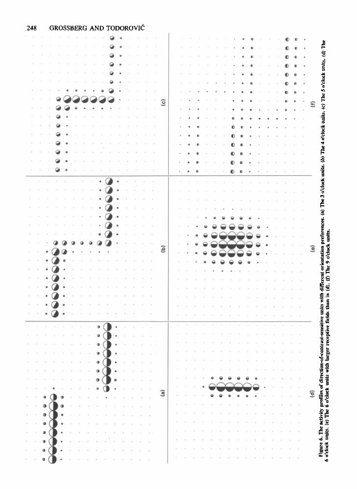
Figure 7a provides a concise symbolism for therepresentation of all 12 Level 3 activity patterns. To construct such a total response profile, we have used a
representation format in which the size of the responseis coded with the length of the clock hand pointing in thedirection of the hour code of a unit. Figure 7b depicts ahorizontally oriented input to Level 3, with stronger activation at the top than at the bottom strip. The responseto such an input would be largest for the optimally tuned3 o'clock unit, weaker for the 2 o'clock and the 4 o'clockunits, weaker still for the I o'clock and the 5 o'clockunits, and zero for the other units. The cluster of linesat the center of Figure 7a concisely represents this pattern of responses at a single position. Since only 5 of the12 units exhibit positive activity, only five clock handsare displayed. The hour to which a hand is pointing codesthe orientation and direction preference of a unit, and thelength of the hand codes response strength.
Figure 8a uses the representationdescribed in Figure 7ato combine the activity patterns of all oriented Level 3units (Figure 6) into a single representation. Each of the16x 16 locations in this representation depicts the activityof 12 units which span the full range of orientation anddirection preferences.
Figure 8b depicts a representation of horizontallyoriented complex cells in Level 4. These cells respondto the sum of output signals from horizontally orientedsimple cells of opposite direction of contrast in Level 3,namely from Figures 6a and 6f. That is why Level 4 cellsdo not have a black hemidisk in their representation.
Figure 8c represents the total activity pattern of allLevel 4 cells using a variant of the representation usedin Figure 8a. In Figure 8c, the activity at a location iscoded by a line centered at it. The activity magnitude isproportional to line length, and the orientation is codedby line orientation. Such a representation was called anorientation field by Grossberg and Mingolla (1985a,1985b).
Figure 8d represents the activity pattern of Level 5units, which compute a total BC output signal from eachBC System position. Each output signal is the sum ofthresholded activities from all the orientations computedat that position in Level 4. The spatial distribution of theactive units traces the Z-shaped stimulus contour. The assymetrical representation of the two corners derives fromthe asymmetrical reaction of the on-field to these corners.A more symmetrical activity profile would have been obtained if the off-unit activity had been taken into account.In particular, the weakening of boundary activity at theupper corner of Figure 8d corresponds to the weakeningof concentric on-unit activity at the corresponding location in Figure 5a. In contrast, this is a site of strong offunit activity in Figure 5b.
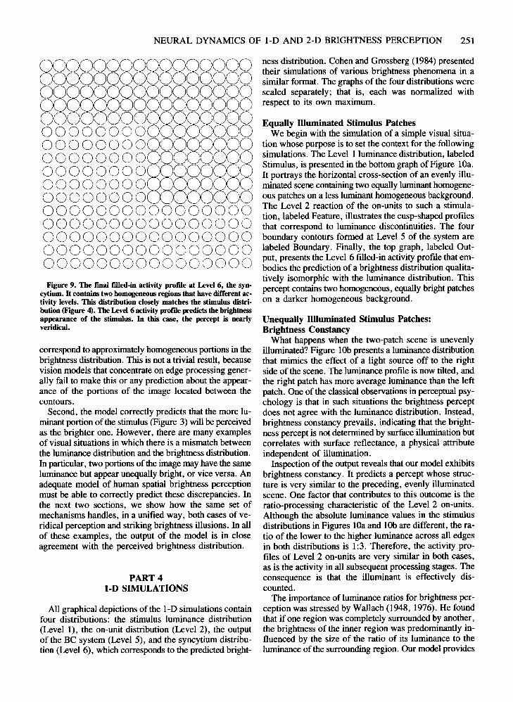
Finally, Figure 9 presents the activitypattern in the fieldof Level 6 units. The BC signal pattern from Level 5 divides the field into two compartments, or interaction domains: the lower left region (yang) and the upper rightregion (yin). Inputs from Level 2 trigger a spreading, orfilling-in, of activity within each domain, but there is little communication between domains. The final activitylevel for points within a domain is roughly proportional

250 GROSSBERG AND TODOROVIC
9
• 6 e e
•• •
.eeeeeeee·eEEjeeeee
e .. a .. ..e e e e e e 9 • • •
eeeeeee
eeeeeeeeeeeeCD3e·~~~~~~~~ "
ff .. ~1'\~
" Jj\ ~~ ~ ~ ~ ~ ~ • ~ 11' ~
........ "'-¥-~..,.11'~
,;If11f\.--..,. ..............~ ~~~~~~~
if
...... ~
• e e e e e e e e6 e e e e e e
(a) (bl
******~~ '\. ... .. .. , \ t
f **. . . . ~ ~ -.. **.... 1,- *.'\ *•-----
'\ ,'*'*******.. ,i ..
Figure 8. (a) The combined activity profile of all Level 3 units. Each cluster of lines represents the activity level of 12 units tbat bavethe same location. The representational codeis described in Figure 7. (b) The activity profile of horizontally oriented direction~-cODtrast
insensitive Level 4 units. Each unit sums the activity of two Level 3 units with the same location and orientation hut opposite directionsensitivity. (c) The combined activity profile of all Level 4 units. Each cluster of lines represents the activity level of six units that havethe same location. Activity magnitode is codedby line length, and orientation preference is coded by line orientation. (d) Level 5: Outputof the Boundary Contour System. Each unit sums the thresholded signal of 6 Level 4 units with the same location. The activity profiletraces the sbared houndary of the two regions of the yin-yang square.
to the average level of input stimulation due to the corresponding Level 2 region. Because of the increased levelof on-units activity on the yin side of the Z-shaped contour, and the decreased level on the yang side, the average activity is smaller within the yang region than in theyin region. The final consequence is that, in Figure 9,the activity pattern of the Level 6 syncytium is qualitatively very similar to that of Figure 4, the image stimu-
Ius distribution, except for modest brightness enhancement and attenuation at the Mach comers of the percept.Since the Level 6 activity profile in our model is the counterpart of the brightness percept, the prediction from thesimulation is that the percept is close to being veridical.
There are two particularly noteworthy aspects of ourintroductory example. First, the two portions of the stimulus distributions that have homogeneous luminance levels
NEURAL DYNAMICS OF l-D AND 2-D BRIGHTNESS PERCEPTION 251
0000000000000000000000000000000000000000000000000000000000000000000000000000000000000000000000000000000000000000oooooooogooooo00000000 0000000000000 0000000000000 000000000000000000000000000000000000000000000000000000000000000000000000000000000000
Figure 9. The final filled-in activity profile at Level 6, the syncytium. It contains two homogeneous regions that have different activity levels. This distribution closely matches the stimulus distribution (Figure 4). The Level 6 activity profile predicts the brightnessappearance of the stimulus. In this case, the percept is nearlyveridical.
correspond to approximately homogeneous portions in thebrightness distribution. This is not a trivial result, becausevision models that concentrate on edge processing generally fail to make this or any prediction about the appearance of the portions of the image located between thecontours.
Second, the model correctly predicts that the more luminant portion of the stimulus (Figure 3) will be perceivedas the brighter one. However, there are many examplesof visual situations in which there is a mismatch betweenthe luminance distribution and the brightness distribution.In particular, two portions of the image may have the sameluminance but appear unequally bright, or vice versa. Anadequate model of human spatial brightness perceptionmust be able to correctly predict these discrepancies. Inthe next two sections, we show how the same set ofmechanisms handles, in a unified way, both cases of veridical perception and striking brightness illusions. In allof these examples, the output of the model is in closeagreement with the perceived brightness distribution.
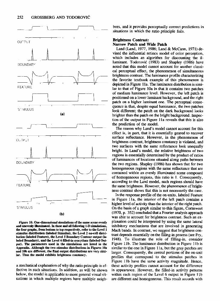
PART 4I-D SIMULATIONS
All graphical depictions of the 1-D simulations containfour distributions: the stimulus luminance distribution(Levell), the on-unit distribution (Level 2), the outputof the BC system (Level 5), and the syncytium distribution (Level 6), which corresponds to the predicted bright-
ness distribution. Cohen and Grossberg (1984) presentedtheir simulations of various brightness phenomena in asimilar format. The graphs of the four distributions werescaled separately; that is, each was normalized withrespect to its own maximum.
Equally Illuminated Stimulus PatchesWe begin with the simulation of a simple visual situa
tion whose purpose is to set the context for the followingsimulations. The Level 1 luminance distribution, labeledStimulus, is presented in the bottom graph of Figure lOa.lt portrays the horizontal cross-section of an evenly illuminated scene containing two equally luminant homogeneous patches on a less luminant homogeneous background.The Level 2 reaction of the on-units to such a stimulation, labeled Feature, illustrates the cusp-shaped profilesthat correspond to luminance discontinuities. The fourboundary contours formed at Level 5 of the system arelabeled Boundary. Finally, the top graph, labeled Output, presents the Level 6 filled-in activity profile that embodies the prediction of a brightness distribution qualitatively isomorphic with the luminance distribution. Thispercept contains two homogeneous, equally bright patcheson a darker homogeneous background.
Unequally Illluminated Stimulus Patches:Brightness Constancy
What happens when the two-patch scene is unevenlyilluminated? Figure lOb presents a luminance distributionthat mimics the effect of a light source off to the rightside of the scene. The luminance profile is now tilted, andthe right patch has more average luminance than the leftpatch. One of the classical observations in perceptual psychology is that in such situations the brightness perceptdoes not agree with the luminance distribution. Instead,brightness constancy prevails, indicating that the brightness percept is not determined by surface illumination butcorrelates with surface reflectance, a physical attributeindependent of illumination.
Inspection of the output reveals that our model exhibitsbrightness constancy. lt predicts a percept whose structure is very similar to the preceding, evenly illuminatedscene. One factor that contributes to this outcome is theratio-processing characteristic of the Level 2 on-units.Although the absolute luminance values in the stimulusdistributions in Figures lOa and lOb are different, the ratio of the lower to the higher luminance across all edgesin both distributions is 1:3. Therefore, the activity profiles of Level 2 on-units are very similar in both cases,as is the activity in all subsequent processing stages. Theconsequence is that the illuminant is effectively discounted.
The importance of luminance ratios for brightness perception was stressed by Wallach (1948, 1976). He foundthat if one region was completely surrounded by another,the brightness of the inner region was predominantly influenced by the size of the ratio of its luminance to theluminance of the surrounding region. Our model provides
252 GROSSBERG AND TODOROVIC
'--- I---L-_ bors, and it provides perceptually correct predictions insituations in which the ratio principle fails.
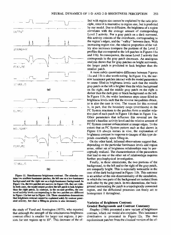
Brightness Contrast:Narrow Patch and Wide Patch
Land (Land, 1977, 1986; Land & McCann, 1971) devised the influential retinex model of color perception,which includes an algorithm for discounting the illuminant. Todorovic (1983) and Shapley (1986) havenoted that this model cannot account for another classical perceptual effect, the phenomenon of simultaneousbrightness contrast. The luminance proftle characterizingthe favorite textbook example of this phenomenon isdepicted in Figure 11a. The luminance distribution is similar to that of Figure lOa in that it contains two patchesof medium luminance level. However, the left patch ispositioned on a lower luminant background, and the rightpatch on a higher luminant one. The perceptual consequence is that, despite equal luminance, the two patcheslook different; the patch on the dark background looksbrighter than the patch on the bright background. Inspection of the output in Figure lla reveals that this is alsothe prediction of the model.
The reason why Land's model cannot account for thiseffect is, in part, that it is essentially geared to recoversurface reflectance. However, in the phenomenon ofbrightness contrast, brightness constancy is violated, andtwo surfaces with the same reflectance look unequallybright. In Land's model, the relative brightness of tworegions is essentially determined by the product of ratiosof luminances of locations situated along paths betweenthe two regions. Shapley (1986) has shown that for twohomogeneous regions with the same reflectance that arecontained within an evenly illuminated scene composedof homogeneous regions, this ratio is 1. Consequently,according to the Land model, such regions should havethe same brightness. However, the phenomenon of brightness contrast shows that this is not necessarily the case.
In the response profile of the on-units, labeled Featurein Figure 11a, the interior of the left patch contains ahigher level of activity than the interior of the right patch.On the basis of a graph similar to this figure, Cornsweet(1970, p. 352) concluded that a Fourier analysis approachwas able to account for brightness contrast. Such an explanation could be interpreted by using the same lateralinhibitory mechanisms that are involved in generatingMach bands. In contrast, we suggest that brightness contrast depends essentially on the filling-in process (see Fry,1948). To illustrate the role of filling-in, considerFigure l lb, The luminance distribution in Figure l lb issimilar to the one in Figure l la, but the gray patches arelarger. Consequently, the central portions of the on-unitproftles that correspond to the stimulus patches inFigure l lb have the same activity magnitude. Hence,these activity proftles cannot account for the differencein appearance. However, the filled-in activity patternswithin each region of the Level 6 output in Figure l lbare different and homogeneous. This result accords with
,---'T------
STIMULUS
BOUNDARY
FEATURE
~~----_.,-----
(8)
SlIMUl.US
(b)
a mechanical explanation of why the ratio principle is effective in such situations. In addition, as will be shownbelow, the model is applicable to more general visual situations in which multiple regions have multiple neigh-
FEATURE
OUTF'UT
BOUNDARY
OUTPUT
Figure 10. One-dimensional simulations of the same scene evenlyand unevenly illuminated. In these and aUfollowing 1-D simulations,the four graphs, from bottom to top respectively, refer to the Level 1stimulus distribution (labeled Stimulus), the Level 2 on-ceU distribution (labeled Feature), the LevelS Boundary Contour output (labeled Boundary), and the Level 6 filled-in syncytium (labeled Output). The parameters used in the simulations are listed in theAppendix. Although the two stimulus distributions in Figures lOaand lOb are different, the fmal output distributions are very similar. Thus the model exhibits brightness constancy.
NEURAL DYNAMICS OF 1-0 AND 2-D BRIGHTNESS PERCEPTION 253
feet with region size cannot beexplained by the ratio principle, since it is insensitive to region size, but is predictedby our model. Due to diffusion, the brightness of a regioncorrelates with the average amount of correspondingLevel 2 activity. For a gray patch on a dark surround,this activity consists of the overshoots, corresponding tothe region's edges, and the "valley" between them. Withincreasing region size, the relative proportion of the valley also increases (compare the portions of the Level 2profiles that correspond to the left patches in Figures 11aand 11b). In consequence, the mean Level 2 activity thatcorresponds to the gray patch decreases. An analogousanalysis shows that for gray patches on bright surrounds,the larger patch is predicted to look brighter than thesmaller patch.
A more subtle quantitative difference between Figures1la and l lb is also worth noting. In Figure 11a, the narrow luminance patches interact with the model parametersto cause filled-in brightness levels such that the middlegray patch on the left is brighter thanthe white backgroundon the right, and the middle gray patch on the right isdarker than the dark gray or black background on the left.In Figure l lb, the wider luminance steps cause filled-inbrightness levels such that the reverse inequalities obtain,as is also the case in vivo. The reason for this reversalis, in part, that the boundary cusps (overshoots) in theFC System reactions to the patches form a smaller relative part of each patch in Figure l lb than in Figure 11a.Other parameters that influence this reversal are themodel's baseline activity level and the relative amount ofFC System contrast enhancement at image edges. To theextent that an FC System pattern such as that shown inFigure l lb always occurs in vivo, the explanation ofbrightness contrast in response to images of this type depends essentially upon filling-in.
On the other hand, informal observations suggest that,depending on the particular luminance levels and regionareas, either set of brightness relationships may be perceptually realized. The characterization of the parametersthat lead to one or the other set of relationships requiresfurther psychophysical investigation.
Finally, in these simulations, the two portions of thebackground, to the left and to the right of the gray patch,are unequally bright. This is especially noticeable in thecase of the dark background in Figure 11b. This outcomeis an artifact of the one-dimensionality of the simulation,in which the two parts of the background are isolated fromeach other by the gray patch. In two dimensions, the background surrounding the patch is a topologically connectedregion, and the diffusional processes can freely act tohomogenize it throughout.
Varieties of Brightness Contrast:Graded Backgrounds and Contrast Constancy
Shapley (1986) presented a new variant of brightnesscontrast, which our model also explains. This luminancedistribution is presented in Figure 12a. The twoequiluminant patches from the classical version of the ef-
u
1t,
STIMULUS
(b)
STIMULUS
- --- .. _. - -r-:---'-'
(a)
____~n'--- ___'
BOUNDARY
OUWUT
----,-~ ~-,
OUTPUT
BOUNDARY
Figure 11. Simultaneous brightness contrast. The stimulus contains two medium luminance patcbes, tbe left one on a low-luminancebackground and the right one on a high-luminance background. InFigure lla, the two patcbes are narrow; in Figure lIb, they are wide.In botb cases, the modeloutput predicts the left patch to look brighterthan the right patch. In contrast, in the on-unit profdes, tbe centered activity levels corresponding to the two patches are differentin Figure lla but not in Figure lIb. These simulations demonstratethat brightness contrast cannot be explained solelyby contour generated activity, but that a filling-in process is also necessary.
the study of Yund and Armington (1975), who reportedthat although the strength of the simultaneous brightnesscontrast effect is smaller for larger test regions, it persists for test regions up to 10°. This decrease of the ef-
254 GROSSBERG AND TODOROVIC
__-------.f\~------_
--~~~--~--~/\~--
OUTPUT
BOUNDAFU
A A,
BOUNDARY
A A,
FEATURE FEATURE
STIMULUS
lal
---r--"\'-- /1L- _
OUTPUT
___---lnL- --, n'-- -...J '---- _
------,----,----r------,----,----r---,-------
STIMULUS
lbl
---!\'---_--lr--------,u---
OUTPUT
A ABOUNDARY BOUNDARY
~-,------:\fIr-,FEATURE
1t,
STIMULUS STIMULUS
lei ldl
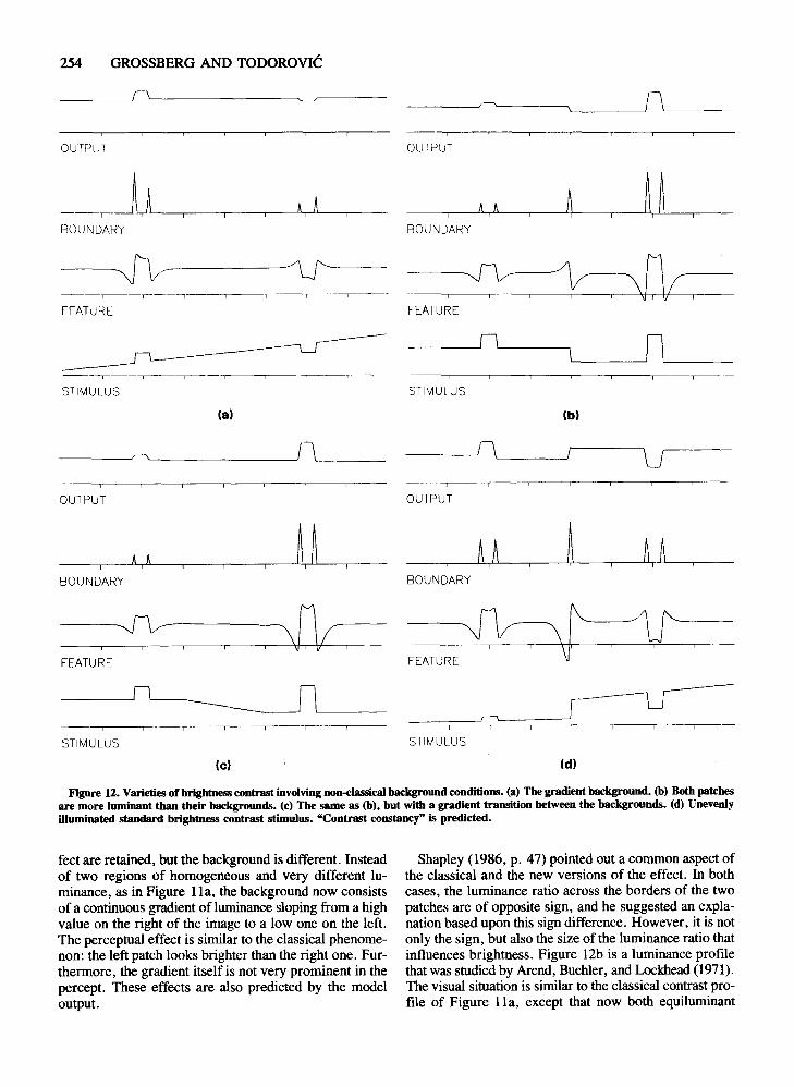
Figure 12. Varieties of brightness contrast involving DOn-classical background conditions. (a) The gradient background. (b) Both patchesare more luminant than their backgrounds. (c) The same as (b), but with a gradient transition between the backgrounds. (d) Unevenlyilluminated standard brightness contrast stimulus. "Contrast constancy" is predicted.
feet are retained, but the background is different. Insteadof two regions of homogeneous and very different luminance, as in Figure lla, the background now consistsof a continuous gradient of luminance sloping from a highvalue on the right of the image to a low one on the left.The perceptual effect is similar to the classical phenomenon: the left patch looks brighter than the right one. Furthermore, the gradient itself is not very prominent in thepercept. These effects are also predicted by the modeloutput.
Shapley (1986, p. 47) pointed out a common aspect ofthe classical and the new versions of the effect. In bothcases, the luminance ratio across the borders of the twopatches are of opposite sign, and he suggested an explanation based upon this sign difference. However, it is notonly the sign, but also the size of the luminance ratio thatinfluences brightness. Figure 12b is a luminance profilethat was studied by Arend, Buehler, and Lockhead (1971).The visual situation is similar to the classical contrast profile of Figure lla, except that now both equilurninant
NEURAL DYNAMICS OF 1-D AND 2-D BRIGHTNESS PERCEPTION 255
BOUNDARY
~~TATURE \J
STIMULUS
(b)
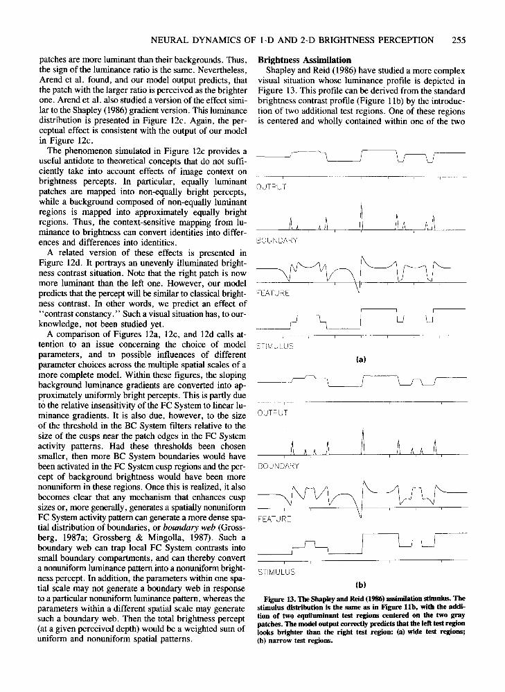
Figure 13. The Shapley and Reid (1986) assimilationstimulus. Thestimulus distribution is the same as in Figure lIb, with the addition of two equiluminant test regions centered on the two graypatches. The model output correctly predicts that the left test regionlooks brighter than the right test region: (a) wide test regions;(b) narrow test regions.
(a)
Brightness AssimilationShapley and Reid (1986) have studied a more complex
visual situation whose luminance profile is depicted inFigure 13. This profile can be derived from the standardbrightness contrast profile (Figure 11b) by the introduction of two additional test regions. One of these regionsis centered and wholly contained within one of the two
OUTPUT
STiMULUS
BOUNDARY
OUTPUT
__~r--
~FEATURE
patches are more luminant than their backgrounds. Thus,the sign of the luminance ratio is the same. Nevertheless,Arend et al. found, and our model output predicts, thatthe patch with the larger ratio is perceived as the brighterone. Arend et al. also studied a version ofthe effect similar to the Shapley (1986) gradient version. This luminancedistribution is presented in Figure 12c. Again, the perceptual effect is consistent with the output of our modelin Figure 12c.
The phenomenon simulated in Figure 12c provides auseful antidote to theoretical concepts that do not sufficiently take into account effects of image context onbrightness percepts. In particular, equally luminantpatches are mapped into non-equally bright percepts,while a background composed of non-equally luminantregions is mapped into approximately equally brightregions. Thus, the context-sensitive mapping from luminance to brightness can convert identities into differences and differences into identities.
A related version of these effects is presented inFigure 12d. It portrays an unevenly illuminated brightness contrast situation. Note that the right patch is nowmore luminant than the left one. However, our modelpredicts that the percept will be similar to classical brightness contrast. In other words, we predict an effect of"contrast constancy." Such a visual situation has, to ourknowledge, not been studied yet.
A comparison of Figures 12a, 12c, and 12d calls attention to an issue concerning the choice of modelparameters, and to possible influences of differentparameter choices across the multiple spatial scales of amore complete model. Within these figures, the slopingbackground luminance gradients are converted into approximately uniformly bright percepts. This is partly dueto the relative insensitivity of the FC System to linear luminance gradients. It is also due, however, to the sizeof the threshold in the BC System filters relative to thesize of the cusps near the patch edges in the FC Systemactivity patterns. Had these thresholds been chosensmaller, then more BC System boundaries would havebeen activated in the FC System cusp regions and the percept of background brightness would have been morenonuniform in these regions. Once this is realized, it alsobecomes clear that any mechanism that enhances cuspsizes or, more generally, generates a spatially nonuniformFC System activity pattern can generate a more dense spatial distribution of boundaries, or boundary web (Grossberg, 1987a; Grossberg & Mingolla, 1987). Such aboundary web can trap local FC System contrasts intosmall boundary compartments, and can thereby converta nonuniform luminance pattern into a nonuniform brightness percept. In addition, the parameters within one spatial scale may not generate a boundary web in responseto a particular nonuniform luminance pattern, whereas theparameters within a different spatial scale may generatesuch a boundary web. Then the total brightness percept(at a given perceived depth) would be a weighted sum ofuniform and nonuniform spatial patterns.
256 GROSSBERG AND TODOROVIC
original equiluminant gray patches; the other is centeredand contained within the other gray patch. The test regionshave the same luminance level, which is higher than theluminance level of surrounding gray patches. However,the experiment showed that the left test region looksbrighter than the right one. A gradient version of this distribution showed similar results.
Shapley (1986) and Shapley and Reid (1986) claimedthat this effect could not be due to brightness contrast,and that it was, instead, an instance of another classicalbrightness effect, the phenomenon of brightness assimilation (Helson, 1963). They pointed out that the ratio ofthe luminance of each of the innermost patches to the luminance of the immediately surrounding region was thesame. Ifclassical brightness contrast were exclusively dueto the luminance ratio, then a new explanatory principlewould be needed to explain the finding. Wallach (1976)also found that, in a series of three nested regions, theratio principle was violated.
Inspection of the output in Figure 13 reveals that ourmodel correctly predicts the difference in brightness between two inner regions. Thus, the model accounts forWallach's ratio principle as well as its violation in morecomplex situations. In particular, the processing by oncell units can lead to either a contrastive or an assimilative brightness effect. The outcome depends upon the total configuration of FC signals that induce the fIlling-inwithin the compartments defined by the BC signals.
In particular, two aspects of the model contribute to thebrightness assimilation effect described by Shapley andReid (1986), one at Level 2 and the other at Level 6. Thefirst is the context-sensitive response of the Level 2 oncells to two or more contiguous luminance steps. The amplitudes of the overshoots and the undershoots, and theexact course of the Level 2 profile corresponding to a luminance step, are influenced by the presence and polarity of nearby luminance steps. In this way, the two backgrounds can differentially affect the test regions evenacross the surrounding gray patches. In particular, theLevel 2 profile corresponding to the right test region inFigure 13a is depressed relative to the left test region. Asreflected in Shapley and Reid's data, this effect of thebackground should decrease with the size of the width ofthe surrounding gray patches.
A second way in which nearby regions can influenceeach other occurs at the diffusion stage. Although thepresence of a boundary between two regions strongly attenuates the interaction between them, it may not annihilate it completely if the strength of BC signals can varysignificantly with the amount of contrast and the spatialscale of the FC patterns, as it does in Figure 13b. If aweak boundary separates two regions with different FCactivity levels, then activity from each region will, to acertain extent, diffuse across the boundary into the otherregion. This process will tend to increase the final filledin activity level in the left test region of Figure 13b andto reduce it in the right test region. This is because theleft test region is surrounded by a region (corresponding
to the left gray patch) whose Level 2 activity profile is,on the average, larger than the average strength of theLevel 2 profile of the region (corresponding to the rightgray patch) surrounding the right test region. Thus, dueto the combined effect of the small size of the test patchesand the large size of the gray patches, the left test pathappears brighter than the right one even though their FCpatterns are similar.
A third factor is the possible influence of multiple spatial scales (Grossberg, 1987b). A small test region maygenerate boundary signals in one scale but not in another.Featural filling-in within the latter scale will thereforecross the perceptual locations subtended by the small testregion. If that region is surrounded by a darker patch,the total filled-in brightness percept, assuming that it isthe weighted sum of the filled-in activity levels across allscales within that region, will tend to be darker.
The Craik-O'Brien-Cernsweet andBrightness Bull~s-Eye Effects
One of the most attractive brightness phenomena is theCraik-O'Brien-Cornsweet effect, or COCE (Cornsweet,1970; see Todorovic, 1987, for a review). One versionof the COCE is presented in Plate 1. Readers unfamiliarwith this effect might suppose that since the left rectangleis brighter than the right rectangle, it is also the more luminant one. However, the luminance of the two rectangles is actually identical, except for a luminance cusp overshoot at the left flank and a luminance cusp undershootat the right flank of the midline. The illusory nature ofthe phenomenon is most easily demonstrated by the oc-
Plate 1 (opposite). The Craik-<>'Brien-Comsweet effect (COCE).The luminance distribution representing this display is shown inFigure 148. The left rectangle looks brighter than the right rectangle although they have identical luminance, except for the cuspshaped profile of their shared vertical border. (From Todorovic,1987.)
Plate 2 (opposite). The 2-D cusp distribution without the bounding contour. This display differs from Plate 1 only with respect tothe background. The dark background in Plate 1 bas been replacedwith a background whose luminance is equal to the average luminance of the two central rectangles. There is no iUusory brightness effect in this display comparable to the COCE in Plate 1 (FromTodorovic, 1983, 1987.)
Plate 3 (p. 259). The impossible brightness staircase. The stimulus distribution corresponding to this display is presented inFigure 20a. The display consists of four L-shaped regions whoseshared borders have a cusp-shaped luminance profile. When thisdisplay is occluded such that only portions of two neighboring regionsare visible (see Figure 21a for an example of the resulting stimulusdistribution), the result is a standard case of the COCE. ITthe occlusion demonstration is carried out for all four neighboring regionpairs, the first member of the pair in the clockwise direction alwaysappears brighter than the second member. In the unoccluded display, no stable pattern of brightness relationships between neighboring regions emerges. (From Todorovic, 1983.)
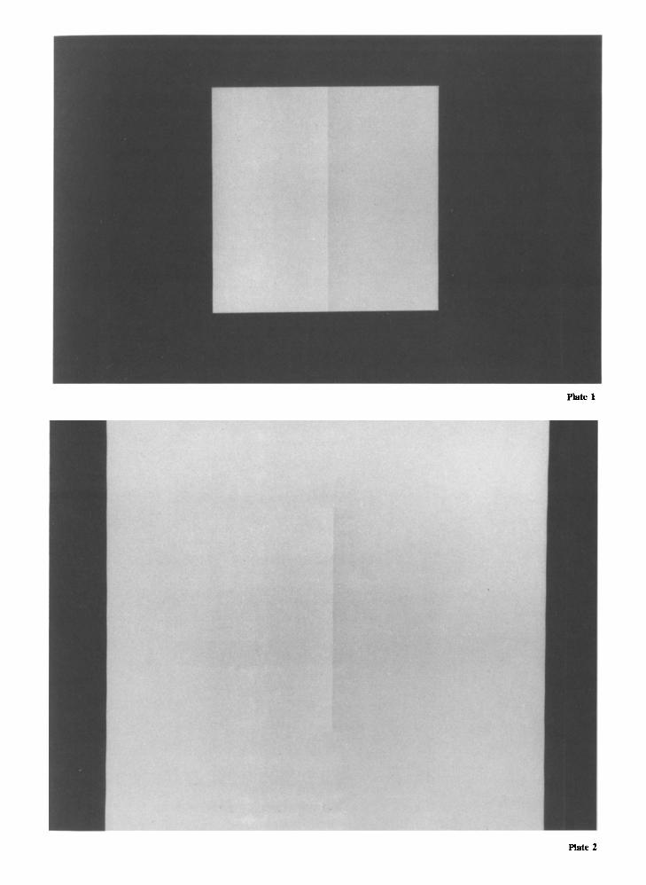
Plate 1
Plate 2
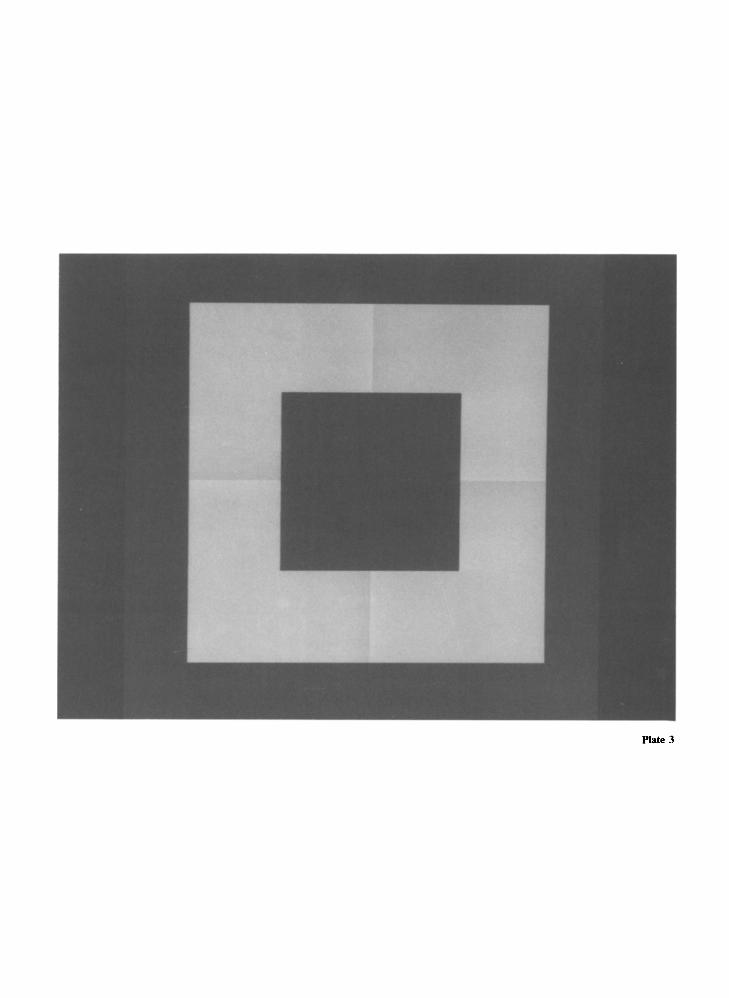
Plate 3

NEURAL DYNAMICS OF 1-D AND 2-D BRIGHTNESS PERCEPTION 261
OUTPUT
BOUNDARY
FEATURE
--~-~---,-----~,--~--·T- ----T---------
STIMULUS
(a)
~----I' ----,--,----,-.-,--~---___________,__---
OUTPUT
BOUNDARY
~r--1r-1r-FEAT~E
-,----,---,----,-----,-----",--------,--
STIMULUS
(b)
Figure 14. The I-D simulations of the COCE and its nonillusorycounterpart. (a) The COCE. (b) A luminance step on a less luminantbackground. The outputs of both simulations predict a step-shapedbrightness profile.
elusion of the contour region. Placing a pencil or a pieceof wire vertically across the midline in Plate 1 causes thetwo rectangles to appear equally bright.
A representation of the 1-D luminance distribution ofa horizontal cross-section of Plate 1 is given in the bottom graph, labeled Stimulus, of Figure 14a. Such a profile includes both the luminance cusps and the equally luminous dark background at the left and right side of thestimulus profile. For comparison, the bottom graph inFigure 14b displays the nonillusory counterpart of the
cusp distribution. It has the form of a simple luminancestep. The cusp distribution and the step distribution areexamples of different stimuli causing similar percepts(Ratliff & Sirovich, 1978). This is also the prediction ofour model presented in the top graphs in Figures 14aand 14b.
The similarity of the perceptual effects of the two images is already apparent in the Level 2 on-eell activity profiles (see Ratliff & Sirovich, 1978, for some related simulations). The loci of abrupt luminance changes in thestimuli induce extended cusp-shaped profiles in the oncell activity pattern, whereas the regions of homogeneous but different luminance induce similar response levels.Some authors have argued that the similarity of activitypatterns at this level, which is also predicted by the Fourier analysis approach, is sufficient to explain the similarity of percepts (Bridgeman, 1983; Cornsweet, 1970;Foster, 1983; Laming, 1983; Ratliff & Sirovich, 1978).Others have been critical of this idea (Arend, 1973; Arend& Goldstein, 1987; Davidson & Whiteside, 1971; Grossberg, 1983; Todorovic, 1983, 1987). The obvious difficulties for such an account are that it does not explain whythe left region is perceived to be brighter than the rightone, or why locations with different activities within thesame region in Level 2 appear to have the same brightness in the final percept.
The model's additional processing stages enable it toexplain both the similarity of the percepts and the shapesof their brightness profiles. This is achieved through themodel's account of how the BC and FC Systems interact. The output of the BC System (Level 5) is presentedin the second graph from the top in Figures 14a and 14b.Only the largest local changes in the Level 2 profiles arereflected in the BC output pattern. The interaction of theLevel 5 BC output and the Level 2 FC output at theLevel 6 syncytium, presented in the top graphs in Figures14a and 14b, predicts the brightness percept. The difference in the activity levels between the left and the rightportions, especially in the case of the COCE, is noticeable but small, but so is the perceived brightnessdifference.
Just as the model can handle multiple steps of differentpolarity, as in Figures 10-14, it can also handle complexstimuli involving several cusp or sawtooth distributionsof different polarities, as shown in Figure 15. Imaginea circularly symmetric 2-D luminance distribution, whoseluminance cross-section along any diameter is given inthe bottom graph of Figure 15a. The appearance of thecentral portion of such a distribution is a brightness bull'seye (Arend, 1973; Arend et al., 1971; Arend & Goldstein, 1987), as predicted by the top graph, labeled Output, in Figure 15a.
This filled-in bull's-eye percept in Figure 15a is generated when the sawtooth luminance pattern is surroundedby a bright background. If the background is sufficientlydark, as in Figure 15b, the difference in brightness between the outermost and the middle band may disappear,as in Figure 15b. Our informal observations of small
262 GROSSBERG AND TODOROVIC
OUTPUT
BOUNDARY
FEATURE
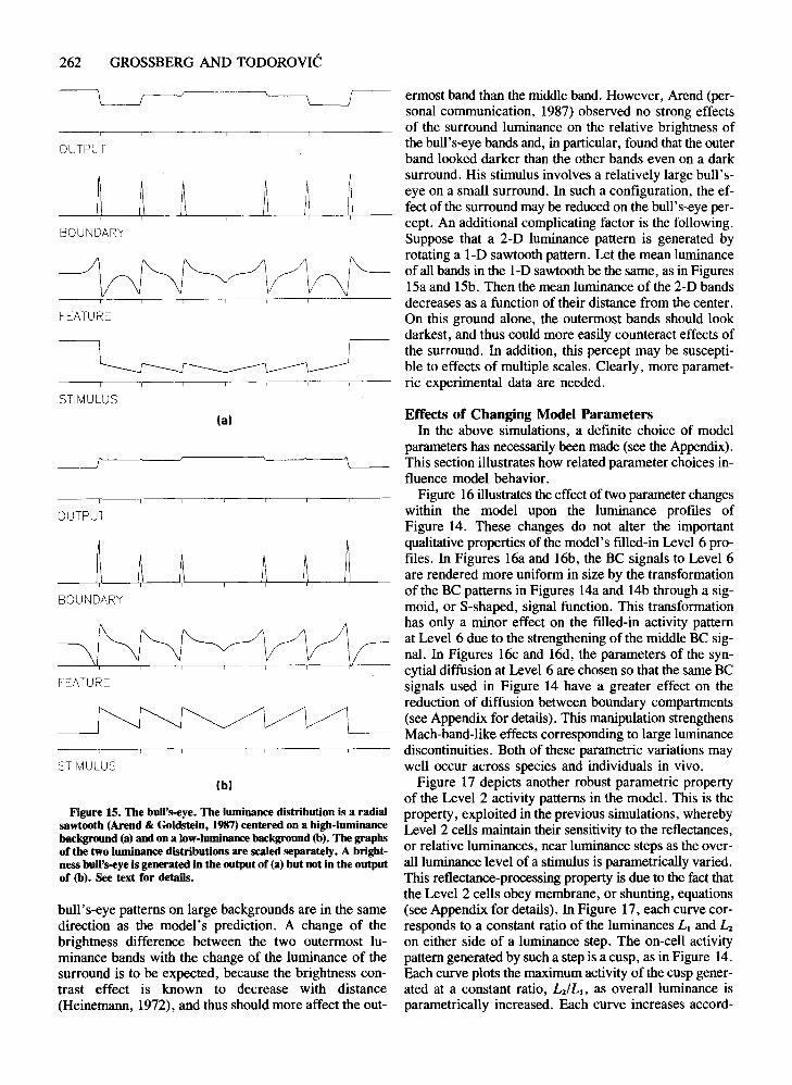
ermost band than the middle band. However, Arend (personal communication, 1987) observed no strong effectsof the surround luminance on the relative brightness ofthe bull's-eye bands and, in particular, found that the outerband looked darker than the other bands even on a darksurround. His stimulus involves a relatively large bull'seye on a small surround. In such a configuration, the effect of the surround may be reduced on the bull's-eye percept. An additional complicating factor is the following.Suppose that a 2-D luminance pattern is generated byrotating a I-D sawtooth pattern. Let the mean luminanceof all bands in the I-D sawtooth be the same, as in Figures15a and 15b. Then the mean luminance of the 2-D bandsdecreases as a function of their distance from the center.On this ground alone, the outermost bands should lookdarkest, and thus could more easily counteract effects ofthe surround. In addition, this percept may be susceptible to effects of multiple scales. Clearly, more parametric experimental data are needed.
STIMULUS
FEATURE
Effects of Changing Model ParametersIn the above simulations, a definite choice of model
parameters has necessarily been made (see the Appendix).This section illustrates how related parameter choices influence model behavior.
Figure 16 illustrates the effect of two parameter changeswithin the model upon the luminance profiles ofFigure 14. These changes do not alter the importantqualitative properties of the model's filled-in Level 6 profiles, In Figures l6a and 16b, the BC signals to Level 6are rendered more uniform in size by the transformationofthe BC patterns in Figures 14a and 14b through a sigmoid, or S-shaped, signal function. This transformationhas only a minor effect on the filled-in activity patternat Level 6 due to the strengthening of the middle BC signal. In Figures l6c and 16d, the parameters of the syncytial diffusion at Level 6 are chosen so that the same BCsignals used in Figure 14 have a greater effect on thereduction of diffusion between boundary compartments(see Appendix for details). This manipulation strengthensMach-band-like effects corresponding to large luminancediscontinuities. Both of these parametric variations maywell occur across species and individuals in vivo.
Figure 17 depicts another robust parametric propertyof the Level 2 activity patterns in the model. This is theproperty, exploited in the previous simulations, wherebyLevel 2 cells maintain their sensitivity to the reflectances,or relative luminances, near luminance steps as the overall luminance level of a stimulus is parametrically varied.This reflectance-processing property is due to the fact thatthe Level 2 cells obey membrane, or shunting, equations(see Appendix for details). In Figure 17, each curve corresponds to a constant ratio of the luminances L. and L,on either side of a luminance step. The on-cell activitypattern generated by such a step is a cusp, as in Figure 14.Each curve plots the maximum activity of the cusp generated at a constant ratio, ~/L.. as overall luminance isparametrically increased. Each curve increases accord-
--_---./'---~-~--"--
(b)
Figure 15. The bull's-eye. The luminance distribution is a radialsawtooth (Arend & Goldstein, 1987) centered on a high-luminancebackground (a) and on a low-luminance background (b). The graphsof the two luminance distributions are scaled separately. A brightness bull's-eye is generated in the output of (a) but not in the outputof (b). See text for details.
bull's-eye patterns on large backgrounds are in the samedirection as the model's prediction. A change of thebrightness difference between the two outermost luminance bands with the change of the luminance of thesurround is to be expected, because the brightness contrast effect is known to decrease with distance(Heinemann, 1972), and thus should more affect the out-
STIMULUS
(a)
---.-f
OUTPUT
-~ ~ ~BOUNDARY

Figure 16. The effects of two parameter changes on simulations in Figure 14. (a, b) Transformation of the Boundary Contour (BC)output through a sigmoid function. (c, d) Increasing the modulation effect of the BC signal on the rilling-in process.
ing to a Weber law property until it asymptotes at an activity level that is characteristic of the ratio ~/Ll (Grossberg, 1983). Thus, large luminance values do not saturatethe on-cell responses. Instead, at large luminances, oncells remain sensitive to input retlectances. The stimulusvalues used in all simulations fall between the dotted vertical lines, and hence within the luminance range of goodratio processing.
PARTSTHE 2-D SIMULATIONS
We now present simulations of brightness phenomenausing the 2-D implementation of the model. A numberof interesting brightness phenomena can be defined anddemonstrated only in two dimensions. Arend and Goldstein (1987) have, in particular, used the curl operator
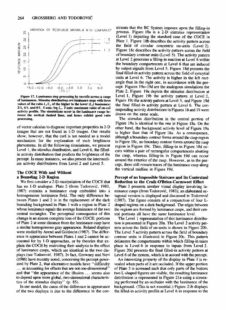
264 GROSSBERG AND TODOROVIC
o+-----";;;;;e~::=::::;.----,--,_-___,_-___,-__.,
-15.0 -12.0 -9.0 -6.0 -3.0 0.0 3.0 6.0LOG Ll
Figure 17. Luminance step processing by on-eeUsacross a rangeof luminances. Stimulus distributions are luminance steps with threevalues ofthe ratio Lz/L. of the higher to the lower (L.) luminance:2/1,4/1, and 8/1. X-axis: log L•. Y-axis: maximum value of on-eellactivity profile. The simulations occur in the luminance range between the vertical dashed lines, and hence exhibit good ratioprocessing.
of vector calculus to diagnose important properties in 2-Dimages that are not found in I-D images. Our resultsshow, however, that the curl is not needed as a modelmechanism for the explanation of such brightnessphenomena. In all the following simulations, we presentLevel 1, the stimulus distribution, and Level 6, the filledin activity distribution that predicts the brightness of thepercept. In many instances, we also present the intennediate activity distributions from Level 2 and Level 5.
The COCE With and Withouta Bounding 2-D Region
We first consider a 2-D manipulation of the COCE thathas no I-D analogue. Plate 2 (from Todorovic, 1983,1987) contains a luminance cusp embedded into ahomogeneous luminance field. The only difference between Plates 1 and 2 is in the replacement of the darkbounding background in Plate 1 with a region in Plate 2whose luminance equals the average luminance of the twocentral rectangles. The perceptual consequence of thischange is an almost complete loss of the COCE: portionsof Plate 2 at some distance from the luminance cusp havea similar homogeneous gray appearance. Related displayswere studied by Arend and Goldstein (1987). The difference in appearance between Plates 1 and 2 cannot be accounted for by I-D approaches, or by theories that explain the COCE by restricting their analysis to the effectof luminance cusps, which are identical in the two displays (see Todorovic, 1987). In fact, Growney and Neri(1986) have recently noted, concerning the percept generated by Plate 2, that alternative models have "difficulty... in accounting for effects that are not one-dimensional"and that "the appearance of the illusion ... seems alsoto depend upon more global, two-dimensionalcharacteristics of the stimulus display" (p. 85).
In our model, the cause of the difference in appearanceof the two displays is due to the difference in the con-
straints that the BC System imposes upon the filling-inprocess. Figure 18a is a 2-D stimulus representation(Level 1) depicting the standard case of the COCE inPlate 1. Figure 18b describes the activity pattern acrossthe field of circular concentric on-units (Level 2).Figure 18c describes the activity pattern across the fieldof boundary contour units (Level 5). The activity patternat Level 2 generates a filling-in reaction at Level 6 withinthe boundary compartments at Level 6 that are inducedby output signals from Level 5. Figure 18d presents thefinal filled-in activity pattern across the field of syncytialunits at Level 6. The activity is higher in the left rectangle than in the right one, in accordance with the percept. Figures 19a-19d are the analogous simulations forPlate 2. Figure 19a depicts the stimulus distribution atLevel 1, Figure 19b the activity pattern at Level 2,Figure 19c the activity pattern at Level 5, and Figure 19dthe final filled-in activity pattern at Level 6. The corresponding activity distributions in Figures 18 and 19 weredrawn on the same scale.
The stimulus distribution in the central portion ofFigure 19a is identical to the one in Figure 18a. On theother hand, the background activity level of Figure 19ais higher than that of Figure 18a. As a consequence,although a boundary contour forms around the cusp regionin Figure 18c, no boundary contour forms around the cuspregion in Figure 19c. Thus, filling-in in Figure 18d occurs within a pair of rectangular compartments abuttingthe cusp, whereas filling-in in Figure 19d can occuraround the exterior of the cusp. However, as in the percept, there still remain traces of the luminance cusp alongthe vertical midline in Figure 19d.
Percept of an Impossible Staircase and Its ContextualReduction to the Craik-O'Brien-Cornsweet Effect
Plate 3 presents another visual display involving luminance cusps (from Todorovic, 1983); an elaborated octagonal version is displayed and discussed in Todorovic(1987). The figure consists of a conjunction of four Lshaped regions on a dark background. The edges betweenthe regions are formed by luminance cusps, and their central portions all have the same luminance level.
The Level 1 representation of this luminance distribution is presented in Figure 20a. The Level 2 activity pattern across the field of on-units is shown in Figure 20b.The Level 5 activity pattern across the field of boundarycontour units is illustrated in Figure 2Oc. This patterndelineates the compartments within which filling-in takesplace in Level 6 in response to inputs from Level 2.Figure 20d presents the final filled-in activity pattern atLevel 6 of the system, which is in accord with the percept.
An interesting property of the display in Plate 3 is revealed when parts of it are occluded. If the upper portionof Plate 3 is screened such that only parts of the bottomtwo L-shaped figures are visible, the resulting luminancedistribution is represented in Figure 21a using a screening performed by an occluder with the luminance of thebackground. (This is not essential.) Figure 21b displaysthe filled-in activity profile at Level 6 in response to the
1-81-4
1-2
VARIATION OF RESPONSE MAXIMUM WITH LUMINANCELf)t'l
0t'l
~:::J Lf)~ NX« 0~ N
W(f) Lf)Z ~
0n,
0(f)W ~
Ci::
L1)
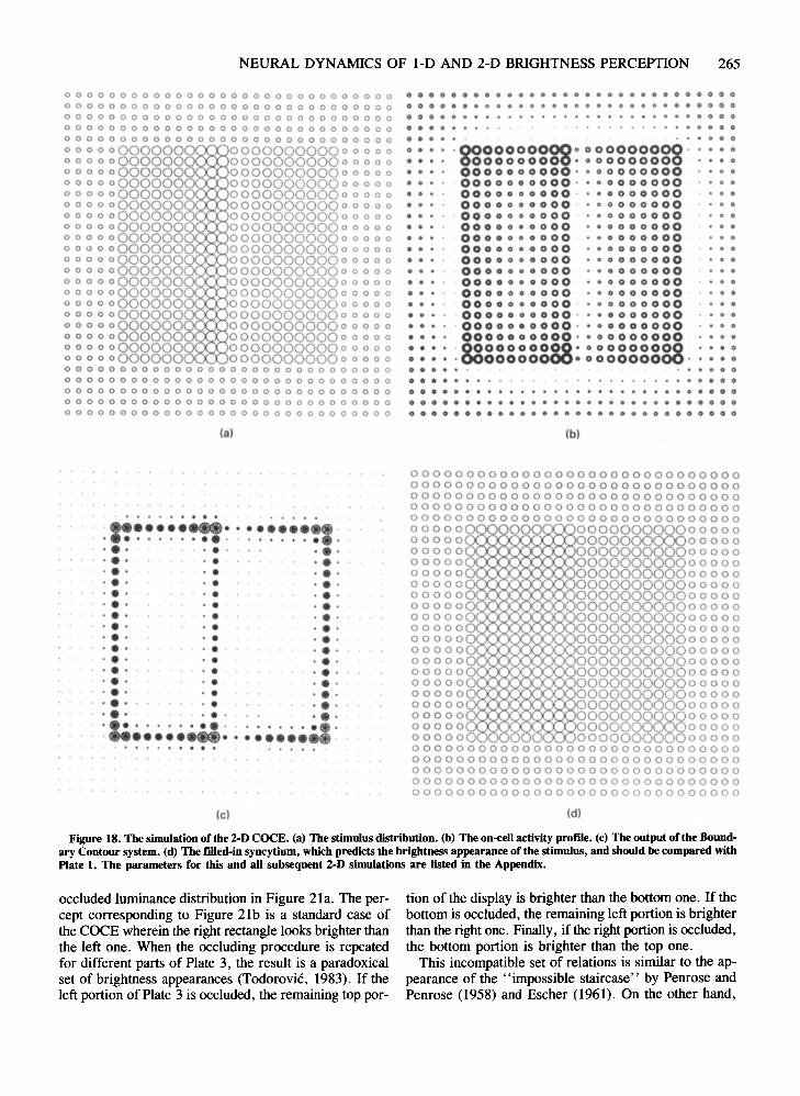
NEURAL DYNAMICS OF I-D AND 2-D BRIGHTNESS PERCEPTION 265
0000000 0 0 0 0 0 0 0 0 0 0 0 0 0 0 0 0 0 0 0 0 0 0 0
o 0 0 000 0 0 0 0 000 0 0 0 0 0 0 0 0 0 0 0 0 0 0 0
00000 •••••••••• 00.... 0000
00000.... . ••.•• 0000
00.' 0000
000. .opooo000000 000000
o 0 000 0 • 0 0 0 0 0 0 0 0 000 0 0 0 0 0 0
o 0 0 0 0 000 0 0 0 0 0 0 0 0 0 0 0 0 0 0 0 0 0 0 0 0 0 0
o 0 0 0 0 0 0 0 0 0 0 000 0 0 0 0 0 0 0 0 0 0 0 0 0 0 0 0o 0 0 0 0 0 0 0 0 0 0 a 0 0 0 0 0 000 0 0 0 0 0 0 0 0 0 0
o 0 0 0 0 0 000 0 0 0 0 0 0 0 0 a 0 0 0 0 0 0 0 0 0 0 0 0o 0 0 0 0 0 0 0 0 0 0 0 0 0 0 0 0 0 0 0 0 0 0 0 0 0 000 0o 0 0 0 0 0 0 0 0 0 0 0 0 0 0 0 0 0 0 0 0 0 0 0 0 000 0 0
000000000000 0000000000 0 0000000000000000 0000000000 0 0000000000000000 0000000000 0 0 000000000000000 0000000000 0 0000000000000000 000000000000000000000000000 0000000000 0 0000000000000000 0000000000 0 0000000000000000 0000000000 0 0 000000000000000 0000000000 0 0000000000000000 0000000000 0 0000000000000000 0000000000 0 0 000000000000000 0000000000 0 0000000000000000 0000000000 0 0000000000000000 000000000000000000000000000 0000000000 0 0000000000000000 000000000000000000000000000 0000000000 0 0000000000000000 0000000000 0 0000000000000000 0000000000 0 0000000000000000 0000000000 0 0000o 0 0 0 0 0 000 0 0 0 0 0 0 0 0 000 0 0 0 0 0 0 0 0 0 0
o 0 000 0 0 000 0 0 0 0 0 0 0 0 0 0 0 0 0 000 0 0 0 0o 0 000 0 0 000 0 a 0 000 0 0 0 0 0 0 0 0 0 0 000 0o 0 000 0 0 0 0 0 0 0 0 0 0 0 0 0 0 0 000 0 0 0 000 0
o 0 000 0 0 0 0 0 0 0 0 0 0 0 0 0 000 0 0 0 0 0 0 0 0 0
000 •
o • 0 •
o • •00.00.o 0
o 0
o 0
00'
00.
o 0
.0'00'
00.
o 0 •
o • •o • •00.
00.
o • •o • • •
'00000000000000000000.0000000000'0000000000000000000' 0000000000000000000' • 00000000 0000000000' 000000000000000000 000000000000000000 000000000000000000 000000000000000000 000000000000000000 000000000000000000 000000000000000000 000000000000000000 000000000000000000 000000000000000000· 000000000000000000' 00000000
-0000000000" 000000000000000000. 0 000000000000000088.000000000
·00000000 0000000000'
<' 000
• 0 0
• 0 0
o 0
o 0
o 0
o 0
• 0 0
• 0
• 0
• 0o 0
o 0
• 0 0
• 0 0/I 000
(a)
.. . , . . ..••.....•~........••... ' .... , ... ..... ' ' ..••• • ••... ...... ...... ..... ' ...... ...... ...... ...... ...... ..... ' ...... ...... ..... ' ...... ' ...•. ' ..... .•.••......~........••
(c)
(b)
00000000000000000000000000000000000000000000000000000000000000000000000000000000000000000000000000000000000000000000000000000000000000000000000000000000000 00000000000000000000 00000000000000000000 00000000000000000000 00000000000000000000 00000000000000000000 00000000000000000000 00000000000000000000 00000000000000000000 00000000000000000000 00000000000000000000 00000000000000000000 00000000000000000000 0000000000000000000000000000 0000000000000000oo00סס000000 0000000000000000000000 000000000000000000000 000000000000000000000 00000000000000000000 000000000000000000000 0000 000000000000000000000000000000000000000000000000000000000000000000000000000000000000000000000000000000000000000000000000000000000000000000000000000000000000000000000
(d)
Figure 18. The simulation of the 2-D COCE. (a) The stimulus distribution. (b) The on-cell activity profIle. (c) The output ofthe Boundary Contour system. (d) The filled-in syncytium, which predicts the brightness appearance of the stimulus, and should be compared withPlate 1. The parameters for this and all subsequent 2-D simulations are listed in the Appendix.
occluded luminance distribution in Figure 21a. The percept corresponding to Figure 21b is a standard case ofthe COCE wherein the right rectangle looks brighter thanthe left one. When the occluding procedure is repeatedfor different parts of Plate 3, the result is a paradoxicalset of brightness appearances (Todorovic, 1983). If theleft portion of Plate 3 is occluded, the remaining top por-
tion of the display is brighter than the bottom one. If thebottom is occluded, the remaining left portion is brighterthan the right one. Finally, if the right portion is occluded,the bottom portion is brighter than the top one.
This incompatible set of relations is similar to the appearance of the "impossible staircase" by Penrose andPenrose (1958) and Escher (1961). On the other hand,
266 GROSSBERG AND TODOROVIC
00000000000000000000000000000000000000000000000000000000000000000000000000000000000000000000000000000000000000000000000000000000000000 000000000000000000000000000 000000000000000000000000000 000000000000000000000000000 000000000000000000000000000 000000000000000000000000000 000000000000000000000000000 000000000000000000000000000 000000000000000000000000000 000000000000000000000000000 000000000000000000000000000 000000000000000000000000000 000000000000000000000000000 000000000000000000000000000 000000000000000000000000000 000000000000000000000000000 000000000000000000000000000 000000000000000000000000000 000000000000000000000000000 000000000000000000000000000 000000000000000000000000000 00000000000000000000000000000 000000000000000000000000000000000000000000000000000000000000000000000000000000000000000000000000000000000000000000000000000000000000000
(a)
· ..• •••• •••• •••••• •• •• •·..
• •••• •• •• •••• •· .
(e)
o Q 0 0 0 0 0 0 0 0 0 000 0 0 000 0 0 0 0 0 0 0 0 0 0 0
o 000 0 0 0 0 0 0 0 0 0 0 0 0 000 000 0 0 0 0 0 0 0 0
000 000 0 0 0 0 0 0 0 0 0 0 0 0 0 0 0 0 0 0 0 0 0 0 0 0
000 0 0 0 Q 0 0 0 000 0 0 0 000 0 0 0 000 0 0 0 0 0
000 0 0 0 0 0 0 0 000 0 0 0 0 0 000 0 0 0 000 000
000000000000000 0000000000000
000000000000000 0000000000000
000000000000000 0000000000000
000000000000000 0000000000000
000000000 0 00000 0 000000000 Q 0 00000000 0 0 0 0 0000 0 000000000 000
0000000000 00000 0 000000000 Q 0 0000000000000000 0000000000000
00000000 0 0 0 0000 0 0000000000 0 0
000000000000000 0 000000000000
000000000000000 0000000000000
0000000000 0 0000 (I 000000000000
0000000000 0 0000 0 000000000000
000000000000000 0000000000000
000000000000000 0000000000000
000000000 0 0 0000 0 000000000000
000000000 0 0 0000 0 000000000000
000000000000000 0000000000000
000000000000000 0000000000000
000000000000000 0000000000000
o 000 0 0 0 0 0 0 0 0 0 0 0 0 0 0 000 0 0 0 000 0 0 0
o 000 Q 0 0 0 0 0 0 0 0 0 0 0 000 0 0 0 000 0 0 0 0 0
000 0 0 0 0 0 0 000 0 0 0 0 0 0 0 0 0 0 0 0 0 0 0 0 0 0
000 0 0 0 000 0 0 0 0 0 000 0 0 000 0 0 0 0 0 000
o 000 0 0 0 0 0 0 0 0 0 0 0 0 000 0 0 0 000 0 0 0 0 0
(b)
COOOWl00 0§fB.0000 00008800 0
~000000880 0 88800 00oooo~8888 ffiSo 0 000000
x
8ID3§0x COO
0 0 x 000
(d)
Figure 19. The simulation of the display in Plate 2. (a) The stimulus disctibution. (b) The on-eell distribution. (c) The output of theBoundary Contour (BC) system. (d) The filled-in syncytium. In contrast to Figure 18, the BC output exhibits no closed compartments.Thus, the filling-process diffuses over the wholeextent of the image and no COCE develops. The stimulus vertical cusp survives in the output.
observation of the whole unoceluded display does not induce stable brightness relations; the L-shaped regions partially lose their homogeneous appearance, and the brightness gradients flanking their shared edges become moreprominent. These observations have been confirmed experimentally in similar displays by Arend and Goldstein(1987). Our model thus predicts in Figure 20d the incon-
elusive appearance of the unoceluded input pattern inFigure 20a, as well as the appearance, in Figure 21b, ofthe COCE in response to the oceluded input pattern inFigure 21a. In addition, the simultaneous brightness contrast effect perceived when Plate 3 is inspected, whichresults in reduced brightness of the inner portion of thebackground, is also obtained in Figure 20d.
NEURAL DYNAMICS OF I-D AND 2-D BRIGHTNESS PERCEPTION 267
000 0 o 000 0
000 • .00 0
000 '00000000880000000000' 000000000000 0000000000 000
o 0 • 00000000880000000000 000000000000 0000000000
o 0 00000000 000000000000. 00000 0000000' 00000 00000o 0 00000 00000 o 0o .. • 00000 88888o 0 o 0 It 0 0 o 0o 0 mgg o 0 000 o 0o 0 o 0 0 0 0o 0 00000 00000 • 0 0o 0 ·00000 00000
00000 00000o 0 0000000000§8o0000000 o 0.. 0 • 000000000 0 00000000000' 00000000 0 0 000000000 o 0000 00000000008800000000 000000 ·0000000000 00000000- o 0 00 000 .00 0
000000000000000000000000000000
o 0 0 0 0 0 0 0 0 0 0 0 0 0 0 0 0 0 0 0 000 0 0 000 0 0
o 0 0 0 0 0 0 0 0 0 0 0 0 0 a 0 0 0 0 0 0 0 0 0 0 000 0 0o 0 0 0 0 0 0 0 000 0 0 000 0 0 0 0 0 0 0 0 0 000 0 0
o 0 0 0 0 coo 0 0 0 0 0 0 0 0 0 0 0 0 0 000 0 000 0 0
000000000000;]000000000000000000000000000 00000000000 0 0 00000000000000 0000000000 0 0000000000000000 000000000000000000000000000 00000000000 00000000000000000000000000000000000000000000000000000000000000000000000000000000000081m0000000000000000000000000 0000000000000000000000000 00000ooooomOOOOOOOOOOOOOOOooooo00000 0000000000000000000000000 000000000000000000000000000000 00000000000000000000000000000000000000000000000000000000000000000;000000000000000000000000000 000000000000000000000000000 000000000000000000000000000 0000000 0 0000000000000000000 00000000 0000o 0 000 0 a 000 0 0 0 0 0 0 0 0 0 0 0 0 0 0 0 a 0 0 0 0
o 0 0 0 0 0 000 0 0 0 0 0 0 0 0 0 0 0 0 0 0 0 0 0 0 0 0 0o 0 000 0 000 0 0 0 0 0 0 0 0 0 0 0 0 0 0 0 0 0 0 0 0 0o 0 000 0 0 0 0 000 0 0 0 0 0 0 0 0 0 0 0 0 0 0 0 0 0 0
o 0 000 0 0 0 0 0 0 0 0 0 0 0 0 0 0 0 0 0 0 0 0 0 0 0 0 0
o 0 0 0 0 0 0 0 Q 000 0 0 0 0 000
o 0 0 000 D 000
000 0
o 0 0 0 •
o 0 0 0 0
000000 00000000
o 0 0 0 0 0 000 000 0 0 0 0
000 0 0 0 0 0 0
00000000
o 0 0 0 0 0
II' 0 000
•• 000000
00000 0
o 0 0 0 0 0 0 0 0 0
(a) (b)
000000000000000000000000000000000000000000000000000000000000000000000000000000000000000000000000000000000000000000000000oooooooooooooooooooooooooooOQO
0000000000610000000000000000oo0סס00000 000000000000000000000000 000000000000000000000000 000000000000000000000000000 000000000000000000000000000000000000000000000ooooooooooooooooooo0oct;000000000000000000000000000 0000000000000000000000000 00000OOOOOmO 00 0 000000000 0000000000 000000000000 000000000000 0000000000000000000000000 000000000000000000000000000 000000000000000000000000000880000000000000000000000000000 00000010000000000000000000000000000 0000000000000000000000000 080000000000000000000000 0 00000000000000000000000 000000000000000000000000000000000000000000000000000000000000000000000000000000000000000000000000000000000000000000000000000000000000000000000000000000000000000000
. '
•••••••••.. '.. '.... .....
• • • ••... ..0:I;~;I:
• •• •• •. .... . . ..
•••• ••••• • ••. .. . . ..... ..'.•.. , ...•••••••••••
••••••••••••••• • •••••••• ••... - ...••• • •••••••... ....• •·. .·. .o~•••~.."..._.••• • ••... .'.' .... ... ....' ..•••••••••
(e) (d)
Figure 20. The simulation of the impossible staircase. (a) The stimulus distribution. (b) The on-cell activity prof"de. (c) The BoundaryContour.JIUtput. (d) The (died-in output.
The Kotl'ka-Benussi RingThe interaction of BCs and the filling-in process are
well illustrated through simulation of the Koffka-Benussiring (Koffka, 1935; Berman & Leibowitz, 1965). The version that we simulate uses a rectangular annulus. The annulus has an intermediate luminance level and is superimposed upon a bipartite background of the same type asin the classical brightness contrast condition, with one half
having a high luminance level and the other half a lowluminance level (Figure 22a). The percept of such a stimulus is that the annulus is approximately uniform in brightness, although the right and the left halves of the annulusexhibit some brightness contrast. This percept correspondsto the Level 6 activity profile in Figure 22b.
The brightness distribution in the percept can bechanged by the introduction of a narrow black line divid-
268 GROSSBERG AND TODOROVIC
o 000 0 0 0 000 0 0 0 0 0 0 0 a 0 0 0 0 a 0 0 0 0 000
o a 0 0 a 0 0 0 0 0 0 0 0 0 0 0 a 0 0 0 0 0 0 0 0 0 0 0 0 0
o 0 0 0 0 0 a a 0 a 0 0 0 0 0 a 0 000 0 0 000 0 0 0 0 0
o 0 000 0 a 0 0 0 0 0 0 0 000 0 0 0 0 0 0 000 0 0 0 0
o 0 0 0 0 0 0 a 0 a 0 0 0 0 a a 0 000 000 000 0 000
o 0 000 0 0 0 0 a 0 0 0 0 0 0 0 0 0 0 0 0 0 0 0 0 0 0 0 0o 0 0 0 0 000 a 000 0 0 0 0 0 0 000 0 a 0 0 0 0 0 a 0o 0 0 0 000 0 0 0 0 0 0 0 0 a 0 0 0 0 0 a 000 0 0 000
o 000 0 0 a 0 0 a 000 0 000 a 0 a 0 0 000 0 0 0 a 0o 000 0 0 0 a a 000 0 0 0 0 0 0 0 a 0 0 0 0 0 0 0 000
a 000 a a 0 0 0 0 a 0 0 0 0 0 0 0 0 0 0 0 0 0 0 0 0 0 0 0
o 0 a 0 a 0 0 000 0 0 0 0 a a 0 0 0 0 0 0 0 0 0 0 0 0 0 0
o 0 000 0 0 0 0 0 0 0 0 0 0 0 a 0 0 0 0 0 0 0 0 0 0 0 0 0
o 000 a 0 0 0 0 0 0 0 0 0 0 a 0 a 000 0 0 000 0 0 0 0
o 0 0 0 a 0 0 0 0 0 0 0 0 0 0 0 0 0 000 0 0 0 0 0 0 0 a 0
o 0 0 0 0 0 a 0 0 0 0 0 a 0 0 0 0 a 000 0 0 000 0 000
o 0 000 000 0 0 0 0 0 0 0 a 0 0 0 a 0 0 000 0 0 0 0 0
o 000 0 0 0 0 a 0 0 0 0 0 0 0 0 0 0 a 0 0 000 0 0 0 0 0
a 000 0 0 a 0 0 0 0 0 0 0 0 0 0 0 0 0 0 0 000 0 0 0 0 0
o 000 0 0 0 a 0 0 0 0 0 0 0 0 0 0 0 0 0 0 000 0 000 0
ooooooooooooooogoooooooooooo000000000000000 000000000000000000000000000 000000000000000000000000000 000000000000000000000000000 000000000000o 000 0 000 0 0 0 0 Q 0 0 0 0 0 0 0 0 0 000 0 0 0 0 0
o 000 0 0 0 0 0 0 0 0 0 0 0 0 0 0 0 0 0 0 000 000 0 0
o 0 0 0 0 0 0 000 0 0 0 0 0 0 0 0 0 0 0 0 000 0 0 0 0 0
o 0 0 0 0 0 0 0 0 0 000 0 000 0 0 0 0 0 000 0 0 0 0 0
o 000 0 0 000 0 0 0 0 0 0 0 0 0 0 0 0 0 0 0 0 0 0 0 0 0
(a)
000000000000000000000000000000000000000000000000000000000000000000000000000000000000000000000000000000000000000000000000000000000000000000000000000000000000000000000000000000000000000000000000000000000000000000000000000000000000000000000000000000000000000000000000000000000000000000000000000000000000000000000000000000000000000000000000000000000000000000000000000000000000000000000000000000000000000000000000000000000000000000000000000000000000000000000000000000000000000000000000000000000000000000000000000000000000000000000000000000000000000000000000000000000000000000000000000000000000000000000000000000000000000 000000000000000000000000000 000000000000000000000 000000000000000000000 0000000000000000000000 0000 0000000000000000000000000000000000000000000000000000000000000000000000000000000000000000000000000000000000000000000000000000000000000000000000000000000000000
(b)
Figure 21. The occluded staircase. (a) The stimulus distribution. (b) The filled-in output. The predicted brightness profile is a standardCOCE.
ing the stimulus vertically into two halves. Figure 22cpresents this new stimulus distribution. In the percept, asin the Level 6 activity profile (Figure 22d), the annulusis now divided into two regions with homogeneous butdifferent brightnesses that are in accord with brightnesscontrast.
These effects depend critically upon interactions between contrast, boundaries, and filling-in in the model.In the unoccludedKoffka-Benussiring, the annular regionat Level 6 is a single connected compartmentwithin whichdiffusion of activity proceeds freely. The opposite contrasts due to the two halves of the background are effectively averaged throughout the annular region, althougha residual effect of opposite contrast remains. The introduction of the occluding boundary (Figure 22c) dividesthe annulus into two smaller compartments (Figure 22d).The different contrasts are now constrained to diffusewithin these compartments, generating two homogeneousregions of different brightness.
Anomalous Brightness DifferentiationOur explanation of the Kanizsa-Minguzzi percept of
anomalous brightness differentiation (Figure I), in whichthe smaller region looks brighter, is consistent with theexplanationof the Koffka-Benussi ring, but also illustratesfiner properties of the model. The critical new property,which does not play a significant role in the percept ofthe Koftka-Benussiring, is that the spokes in the luminouswheel between the black inner and outer regions induceFC signals as well as BC signals. The FC signals are relatively small relative to those induced by the thick black
inner and outer regions. Hence, the perceived brightnessdifference is small. The BC signals induced by the spokedivide the wheel-shaped FC System syncytium into twofilling-in domains of unequal size. Due to the averagingproperty of the diffusive filling-in process, the smallerdomain possesses a larger average activity than the largerdomain. This is because its FC signals due to the spokesare averaged over a smaller region, whereas the FC signals induced by the inner and outer black regions areequally well averaged within each domain. Figure 23presents the simulation of a rectangular version of theKanizsa-Minguzzi stimulus distribution (Figure 23a) andthe filled-in Level 6 activity profile (Figure 23b).
It is instructive to contrast the model properties that giverise to the Koffka-Benussi percepts and the KanizsaMinguzzi percept. In the Koffka-Benussi percepts, thecontrasts induced by the background (Figures 22a and 22c)are asymmetric with respect to the figure and massive dueto their extent along the figure perimeter. The main effect of the thin vertical line (Figure 22c) is to induce anew BC which divides the figure into two filling-in domains of equal size. The FCs caused by this vertical lineare swamped by the filled-in contrasts induced by thebackground within these equally large regions. In theKanizsa-Minguzzi demonstration (Figure 23), the contrasts induced by the background are symmetric withrespect to the figure. On the other hand, the additionallines divide the figure into unequal filling-in domains.Hence the influence of these lines as inducers of FC signals can cause a perceived, albeit small, brightnessdifference.
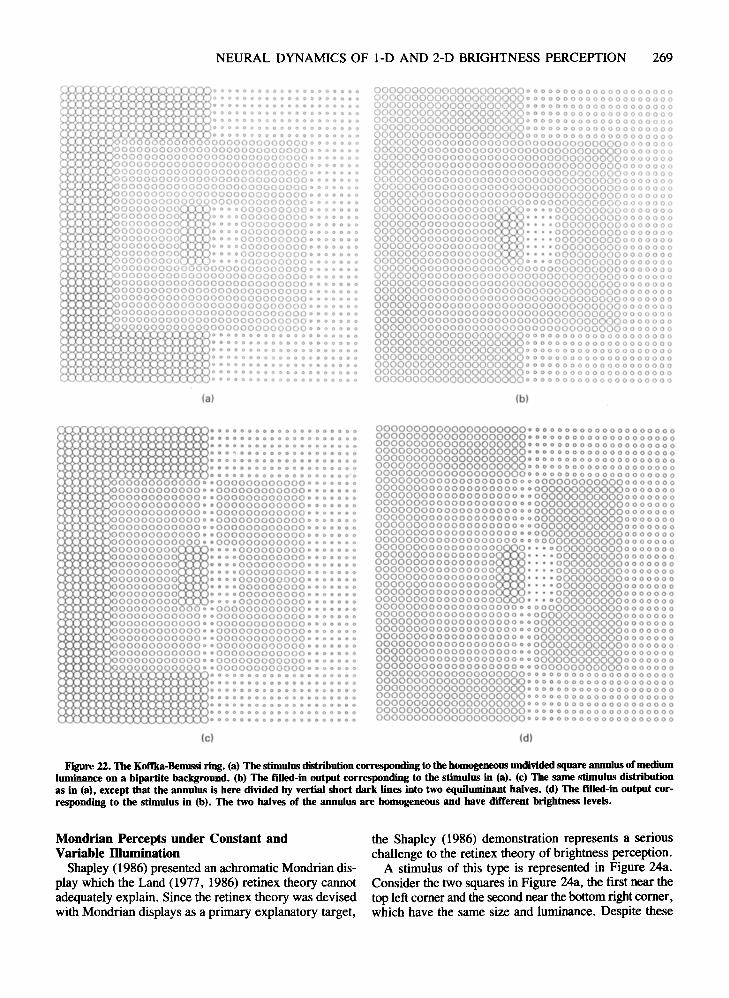
NEURAL DYNAMICS OF 1-D AND 2-D BRIGHTNESS PERCEPTION 269
1111111111111111°0000000000000000000
0000 0 000 0 0000 0 000000
00000 000 0:> 0000 0 ODo 0 00
00000000000000000000
00000000000000000000
0000000000000 0 000 0 00
00000000000000000000
00000000000000000000000000 0 0 0000000000000000000000000000000000000000000000000000000000000000000000000000000000000000000000000000000000000000000000000000000000 0 0 00000
!~~f~~O o o o o o o o o o o o o o o o o o o o o o o o o o o o o o o o o000000000000000000000000000000000
000000000000000000000000000000000000000000000000000000000000000000
gggggggggl::::ggggggggg:::::::N~~N~OOOOOOOOO 00000000000000000000
!~~f~~O O OO OOO O O 00000000000000000000000000000 00000000000000000000
000000000 00000000000000000000000000000 00000000000000000000000000000 0000000000000000000000000000000000000000000000 0 0 00000
00000000000000000000000000 0 0 00000OOOOOOOOOOOOOOOOOOOOOOOOOOvoooooo00000000000000000000000000 0 0 00000000000000000000000000000000000000000000000000000000000000000000000000000000000000000000000000000000000000000000000000000000000000000
0000000000000 0000 0000000000000(>00000000000000000000000 0000 000000000000000000000000000000000000000000
0000 0 000 a 0000 0 0000 00
00000000000000000000
(a)
0000000000000000000000000000000000000000000000000000000000000001") 0 0000000000000000OOOOOOOOGOOOOOOooooo
0000000000000000000000000 0 0 0 0 0 000 0 0 0 0 0 0'0
000000000000 0 0000000000000 0 000000000000000000 0 00000000000000000000000000000000 0 000000000000000000000000000000000000000000000000000000000000000000 0 00000000000000000000000000000000 0 00000000000000000000000000000000000000000000000000000000000000000000000000000000000000000000000000100000000000000000000000000000 00000000000000000000000000000 00000000000000000000000000000 00000000000000000000000000000 00000000000000000000000000000 00000000000000000000000000000 00000000000000000000000000000 00000000000000000000000000000000000000000000000000000000000000000000000000000000000000000000000000 0 00000000000000000000000000000000 0 00000000000000000000000000000000000000000000000000000000000000000000000000000000000000000000000000 0 00000000000000000000000000000000 000000000000000000000000000000000 0 00000000000000000000
00000000000000000000000000000000000000000000000000000000000000000000000000000000o 0> 0 0 0 0 0 .0 0 0 0 0 0 0 0 0 0 0 0 0
o>oa-oo 000 00000000-00000-00000-00000000.000000
(e)
00000000000000000000 0000000000000000000000000000000000000000 0 000000000000000000000000000000000000000 0 0 00000000000000000000000000000000000000 0000000000000000000000000000000000000000 0 000000000000000000000000000000000000000000000000000000000000000000000000000000000000000000000000000000000000000000000000000000000000000000000000000000000000000000000000000000000000000000000000000000000000000000000000000000000000000000000000000000000000000000000000000000000000000000000000000000000000000000000000000000000000000000000000000000000000000000000000000000000000000000000000000000000000000000000000000000000000000000000000000000000000000000000000000oooooooooooooooomooooooooooooooooooooo0000000000000000 ••• 000000000000000000000000000000000 •••• 00000000000000000000000000000000 •••• 00000000000000000000000000000000 • ••• 00000000000000000000000000000000 •••• 00000000000000000000000000000000 ••• 0000000000000000000000000000000000 00000000000000000000000000000000000000000000000000000000000000000000000000000000000000000000000000000000000000000000000000000000000000000000000000000000000000000000000000000000000000000000000000000000000000000000000000000000000000000000000000000000000000000000000000000000000000000000000000000000000000000000000000000000000000000000000000000000000000000000000000000000000000000000000000000000000000000000000000000000000000000000000000000000000000000000000000000000000000000000000000000000000000000000000000000000000000000 0000000000000000000000000000000000000000 0 0 0 0000000000000000000000000000000000000 0 0 0 0000000000000000000000000000000000000 00000000000000000000
(b)
00000000000000000000 0000000000000000000000000000000000000000 0 0 00000000000000000000000000000000000000 0 0 0 0000000000000000000000000000000000000 0000000000000000000000000000000000000000 0 0 0 0000000000000000000000000000000000000. 000000000000000000000000000000000000000 0 0 0000000000000000000000000000000000000 000000000000000000000000000000000000000 0 0 000000000000000000000000000000000000000 0000000000000000000000000000000000000000 0000000000000000000000000000000000000000 000000000000000000000
0000000000000000000 0000000000000000000000000000000000000000 0000000000000000000000000000000000000000 000000000000000000000
0000000000000000000 00000000000000000000000000000000000001°0.0000000000000000000000000000000000 •••• 00000000000000000000000000000000 ••• 000000000000000000000000000000000 •••• 00000000000000000000000000000000 •••• 00000000000000000000000000000000 •••• 00000000000000000000000000000000 •••• 000000000000000000000000000000000 00.0000000000000000000000000000000000000 0 000000000000000000000000000000000000000 0000000000000000000000000000000000000000 0000000000000000000000000000000000000000 0000000000000000000000000000000000000000 000000000000000000000000000000000000000 0 0000000000000000000000000000000000000000 000000000000000000000
0000000000000000000 0000000000000000000000000000000000000000 000000000000000000000000000000000000000000000000000000000000000000000000000000000 0 000000000000000000000000000000000000000 0000000000000000000000000000000000000000 0 0 00000000000000000000000000000000000000 0000000000000000000000000000000000000000 0000000000000000000000000000000000000000 0 0 000000000000000000
(d)
Figure 22. The Koftlw-Benussiring. (a) The stimulus distribution corresponding to the homogeneousundivided square annulus of mediumluminance on a bipartite background. (b) The f"illed-in output corresponding to the stimulus in (a). (c) The same stimulus distributionas in (a), except that the annulus is here divided by vertial short dark lines into two equiluminant halves. (d) The f"illed-in output corresponding to the stimulus in (b). The two halves of the annulus are homogeneous and have different brightness levels.
Mondrian Percepts under Constant andVariable Illuminatton
Shapley (1986) presented an achromatic Mondrian display which the Land (1977, 1986) retinex theory cannotadequately explain. Since the retinex theory was devisedwith Mondrian displays as a primary explanatory target,
the Shapley (1986) demonstration represents a seriouschallenge to the retinex theory of brightness perception.
A stimulus of this type is represented in Figure 24a.Consider the two squares in Figure 24a, the first near thetop left comer and the second near the bottom right comer,which have the same size and luminance. Despite these
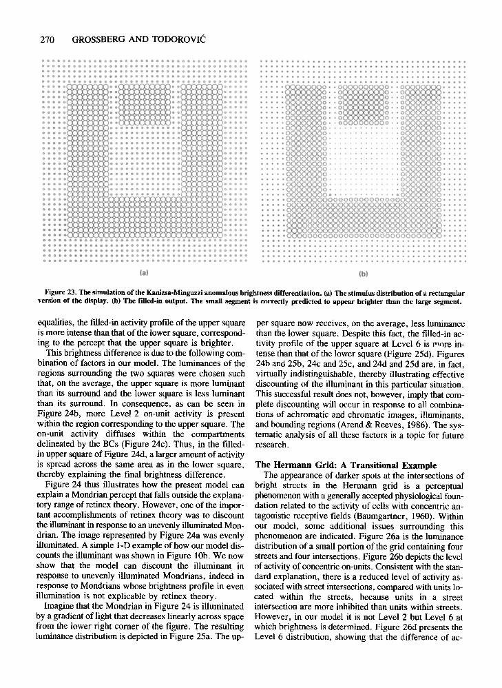
270 GROSSBERG AND TODOROVIC
00000 O{)QOD
00000 OOO()O
o 0 Q 0 0
00000 00000
00000 00000
00000 OOO()O
Q 0000 0 0 ()OOO 0 00 0 CI' a 0 0 0 o Cl'0 0 0 ()O 0 0 0 0 0 0 o 0 0 0 0",0
o Q 00 000 IJ 0 0 Q Q GOO 0 00 0 Q GOO 0 Q 0 6 0 0 0 a 0 <;1 0 0 0 0 0 00
OOQGOOQOOOOOOQOOOOOOOOo-O",OOOOOooooooOaoo
00000000000000000000000.:1000000000000 0000
0000000000000000000000000000000000000000
00000000000000 •••••••••••• 00000000000000
00000 •••• o. 0 •••• 0 ••••• 0 •••••• 0 •• 000001100
00 .. 00.00000.00.0 0 00 0
oo oo oO~
000000.000 0 •• 000 0000000000.
••••• 0 .. 00.000O' '0lm0••••..•••• 0··0 0"0 .•.•.· ••• ·0 O· ·0 O· • 00 .•..•• •.•• 0 g 00 .. 0 0 .. 000 0 ..•..·····0 00. ·0 O· • 00088800 .. '"• •.•. 000 00' . 0 O' . 000 000·····••• "00000000' -0 0··00000000· .• ·...... oggo§§oo. -0000000000· .ooogoooo .· 0 00 000 00· .· ooog 000' 00008800 ....•• •..• 00000000' . . - 00000000· .• ...• 00000000' . . . . . - 00000000· .· 00000000 - . . . . . . . . . . . .. 00000000· .· 00000000' 00000000· .• ...• 00000000 . . . . . . . . . . . . . '00000000· .· oooogooo. . .. , , . . . . . . . . 00000000· ...•· 0000 000' . . . . . , . , , . 00000000· .· 00000000' . . . . . , .. 00000000· .... "00000000" . '00000000·· ..•• .•.• 00000000' . . . . . 00000000· .• 00000000' . . ..... 00000000· .· 00000000 0 •••••••••••• ·00000000· .•. ···000000000000000000000000000000·.········000000000000000000000000000000·.···••••• ;0000000000000000000000000000 ....•·····0 oooooo§gogoooogoooooooooooo .·····0 00000 00000 ooooooooogo .• • • • • 000000 000000000000000000 .•.••• • • • • 0000000000000000000000 .....·····0 000000000000000000000000 0·····
o 0 0 0 co I) 0 0 0
o 0 0 0 0
o 0 0 0 0
o 0 0 0 Q
o 0 0 0 0
o 0 0 0 0
o 0 0 0 0
o 0 0 0 0
o 0 0 0 0
o 0 0 0 0
o 0 0 0 0
o 0 0 0 0
o 0 0 0 0
o 0 0 0 0
o 0 0 I) Q.
o 0 0 0 0
o 0 0 0 0
o 0 0 0 0
o 0 0 0 0
o 0 0 0 0
o 0 0 I> 0
000000000000 c 00 0 0 00 0 0 000 0 0 00 0 000 0 0 0 0 0 0 0 0
000 OQO 0 0 00 0 0 0 00 0 0 00 00 00 0 00 0 0 0 0 00 0 0 0 0 0 0 0 0
00000000000000000 () 0 0 0 00 0 0 0 0 0 0 00 0 0 0 0 0 0 0 0 0
0'0000000000 00000 0 00 0 0000000000000 0 0 o 0 000
OOQOOO(JOOOOOOOQOOOOOOOOOOOOOOOOOOOOOOOOO00000 00.0010000000000 00 00 00000OOODQ 00 00 00000
00000 00 00 OOOGO
00000 00 00 00000
OOO!)O DO 00 00000
o 0 D 0
o 0 0 0
OOO{)OOOOQQOQOO
00000000000000
00000000000000
00000000000000
00000000000000
OOOC)OOOOQOOOOO
OOOC>OOQOOOOQOO
00000000000000
00000000000000
OOQ{)OaOOOOOQOO
00000000000000
OOO()OOOQOOOOOO
000000000000000
00000001>000000
(a) (b)
Figure 23. The simulation ofthe Kanizsa-Minguzzi anomalous brightness differentiation. (a) The stimulus distribution of a rectangularversion of the display. (b) The filled-in output. The small segment is correctly predicted to appear brighter than the large segment.
equalities, the filled-in activity profile of the upper squareis more intense than that of the lower square, corresponding to the percept that the upper square is brighter.
This brightness difference is due to the following combination of factors in our model. The luminances of theregions surrounding the two squares were chosen suchthat, on the average, the upper square is more luminantthan its surround and the lower square is less luminantthan its surround. In consequence, as can be seen inFigure 24b, more Level 2 on-unit activity is presentwithin the region corresponding to the upper square. Theon-unit activity diffuses within the compartmentsdelineated by the BCs (Figure 24c). Thus, in the filledin upper square of Figure 24d, a larger amount of activityis spread across the same area as in the lower square,thereby explaining the final brightness difference.
Figure 24 thus illustrates how the present model canexplain a Mondrian percept that falls outside the explanatory range of retinex theory. However, one of the important accomplishments of retinex theory was to discountthe illuminantin response to an unevenlyilluminatedMondrian. The image represented by Figure 24a was evenlyilluminated. A simple I-D example of how our model discounts the illuminant was shown in Figure lOb. We nowshow that the model can discount the illuminant inresponse to unevenly illuminated Mondrians, indeed inresponse to Mondrians whose brightness profile in evenillumination is not explicable by retinex theory.
Imagine that the Mondrian in Figure 24 is illuminatedby a gradient of light that decreases linearly across spacefrom the lower right comer of the figure. The resultingluminance distribution is depicted in Figure 25a. The up-
per square now receives, on the average, less luminancethan the lower square. Despite this fact, the filled-in activity profile of the upper square at Level 6 is roore intense than that of the lower square (Figure 25d). Figures24b and 25b, 24c and 25c, and 24d and 25d are, in fact,virtually indistinguishable, thereby illustrating effectivediscounting of the illuminant in this particular situation.This successful result does not, however, imply that complete discounting will occur in response to all combinations of achromatic and chromatic images, ilIuminants,and bounding regions (Arend & Reeves, 1986). The systematic analysis of all these factors is a topic for futureresearch.
The Hermann Grid: A Transitional ExampleThe appearance of darker spots at the intersections of
bright streets in the Hermann grid is a perceptualphenomenon with a generally accepted physiologicalfoundation related to the activity of cells with concentric antagonistic receptive fields (Baumgartner, 1960). Withinour model, some additional issues surrounding thisphenomenon are indicated. Figure 26a is the luminancedistribution of a small portion of the grid containing fourstreets and four intersections. Figure 26b depicts the levelof activity of concentric on-units. Consistent with the standard explanation, there is a reduced level of activity as··sociated with street intersections, compared with units located within the streets, because units in a streetintersection are more inhibited than units within streets.However, in our model it is not Level 2 but Level 6 atwhich brightness is determined. Figure 26d presents theLevel 6 distribution, showing that the difference of ac-
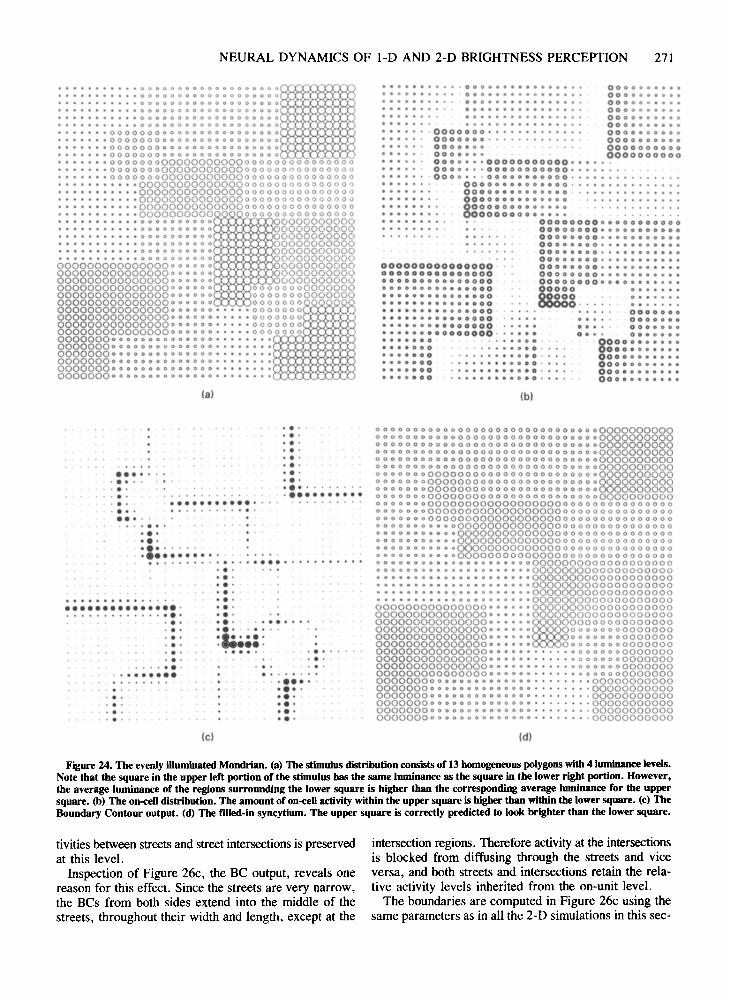
NEURAL DYNAMICS OF I-D AND 2-D BRIGHTNESS PERCEPTION 271
0000000000
0000000000
00000<>000 •000000.000 e0000000000
000000 e 000
00000000000000000000
00000000000000000000
00000000.. 000000000.. 0000000000> 0000000
·00000000000
0000000.0000000 0 0 0 0 0 0 0
0000000 •• 0.0000 0 0 (I 0 0 0 0.000000(1000.
..•• a 0
• 000
0 •• 00·
·00000000000.00.0
ooo-OOOOOOODOOO",
000 •• 0000000000000 •• 0000000 •• 0
00 ••• 00000000.0
.••• 00 •• 000·•• ••••• 0000·
• •••• 0.0000·
•• ••• 0.0000'
·0000000.0000000· •••••••••••0000000000000.00000 0 •• 00000000000 ••••0000. 0.00000000000.
-0000 •• '00000000000.00000000000000'000000000000000000000000000.
80 0 0 0 0 0 0 0 0 0 0 0 00000000000000 ••
0000000000000000000000000000000000000.00000000.000000000000000000 •• 00 0 0 0 0 0 0 0
·00000000.0.00000000
00000000. It. 0 • 0 0 0000
00000000" 0 0 0 • 0 • 0 .. 0 ..
00000000000000000000000000000000000.0.
·00000 00 •••••
88888... :::::::
.000..00ltCOOOoDDO
COOODoco
o 0 0 0 0 co
• 0 0 0
• ••• 0 •·.....
000000000000000·000000000000000000000000000000·00000000000000000000000000000000 ••••• 00000000
•••••••• 000.000·••••• 000.000000·
•••• 00000000000•••• 00000000000·• ••• 0 0 0.000000.000000
..000000..00000••• 0000-
: : : : : ~ ~ : ~ : ~ : : ~ ~ : :: : ~ : : ~:......... 00000000000000000000
...... I> 00000000000000000000
.... 0" 00000000000000000000
........ 00000000000000000000
"00000000000000000000000
000000000000000000000000
oOOQOOOOoooooooooooooooo000000000000000000000000
• 0000000000000000000000000000000000000000000000000000000000000000000·000000000000000000000000000000000
·00000000000000000000000000000···00000000000000000000000000000
·····00000000000000000000000000000·····00000000000000000000000000000
• ·0000000000 00000000000000000000000000000 000000000000 .. 0·0000000000 0000000000000 •• 0000000000 0000000000000000000000000 0000000000000000000000000 00000000000".0.0000000000 00000000000
000000000000000000000 00000000000000000000000000000000 00000000000000000000000000000000 00000000000000000000000000 000000 00000000000000000000000000000000000 00000000000000000000000000000000000 0000000 0000000000000000000000. .0000000q~R~~
OOOOOOOOOOOOOOOOOOOOO ••••• OOO!OIO~O!O~~~~jJ000000000000000000 000 ••••• 0000000000000000000000000000·····0000000000000000000000000000 •••
0000000 0 0 0 0 0 0 0 0 0 0 0 0 0 0 0 •
0000000 0 0 0 0 0 0 0 0 0 0 0 0 0 0 0 •
000000000000000000000 ....OOOOOOOoooooooooooOQOO0000000000000 000000000
••••••••••••, ....... '••••••••••••••
•••••.•.........•... '
·.'......·..·...........0 ••••••••••
• ••••••••••
(bl
0000000 0 0 0 000000000000000000000000000000000000000000000000000000000000000000000000000000000000000000000000000000000000000000000000000000000000000000000000000000000000000000000000000000000000000000000000000000 0 0 0 000000000000000000000000000000000000000000000000000000000000000000000000000000000000000000000000000°8°00000000000000000000000000000000000000 000000000000 0 0 0000000000000000000000000000000000000 000000000000000000000000000000000000000000000000000000000000000000000000000000000000000000000000000000000000000000000ooooococoooooooooooooooooooooooooooooooo0000 0 0 0 0000000000000000000000000000000000000000000000000000000000000000000000000000000000000000000000000000000000000000000000000000000000000000000000000000000000000000000000000000000000000000000000000OOOOOOOOOOOOOOOltOOOltOOOOoooooooooooooooo0000000000000000000<>00000000000000000000• •••••••••• 0··· ••••• ·0000000000000000000OltOOOOOOltoo.ooooooooooOoooooooooooooooooo• ••• 0 •••••• 000···.·.·0000000000000000000000000000000000······0000000000000000000000000000000000 0 ••••• 0000000000000000000000000000000000 0 •••• 0 0 0 0 0 0 0 0 0 0 0 0 0 0 0 0 0 0 0 0oooooooooooooooo ••• oomoooooooooooooooo000000000000000000.00 0000000000000000000000000000000 ••• 0. 00000000000000000000000000000000000 •.•. "000000000000000000000000000000 0 0 • 0 • , 0 0 0 0 0 0 00000000000000000000000000.0. '00000000000000000000000000000000000 00000000000000000000000000000000000 -00000000000000000000000000000000 '0000000000000000000000000000000 0• ·00000000000000000000000000000000. '00000000000000000000000000000000. '00000000000000000000000000000000. '00000000000
........
....... '·..·.'...·..·.'.. '.. . .. ...•••..~ ... "............
(a}
••••' ....., ... .'' ..•••
, .'
, ....'' .....
•••••••
, ..
, ......., ..
••••••••••••••••.................' ..
(e) (dl
Figure 24. The evenly illuminated Mondrian. (a) The stimulus distribution consists of 13 homogeneous polygonswitb 4 luminance levels.Note tbat the square in tbe upper left portion of tbe stimulus bas tbe same luminance as the square in the lower right portion. However,tbe average luminance of tbe regions surrounding tbe lower square is higher than tbe corresponding average luminance for tbe uppersquare. (b) The on-eeU distribution. The amount of on-eeU activity within the upper square is higher than within the lower square. (c) TheBoundary Contour output. (d) The filled-in syncytium. Tbe upper square is correctly predicted to look brighter tban the lower square.
tivities between streets and street intersections is preservedat this level.
Inspection of Figure 26c, the BC output, reveals onereason for this effect. Since the streets are very narrow,the BCs from both sides extend into the middle of thestreets, throughout their width and length, except at the
intersection regions. Therefore activityat the intersectionsis blocked from diffusing through the streets and viceversa, and both streets and intersections retain the relative activity levels inherited from the on-unit level.
The boundaries are computed in Figure 26c using thesame parameters as in all the 2-D simulations in this sec-
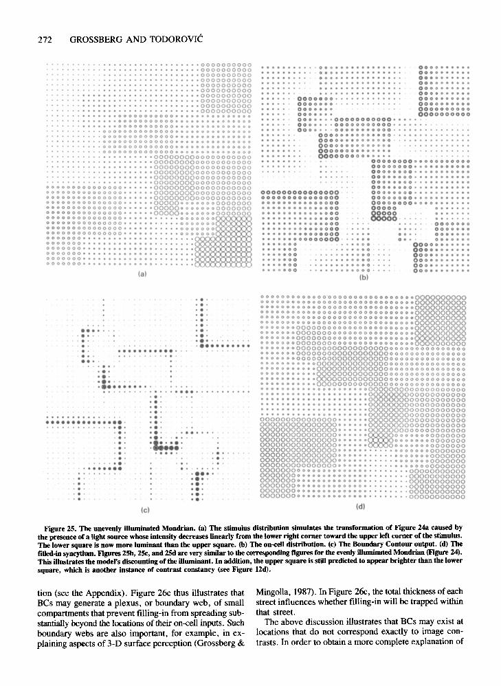
272 GROSSBERG AND TODOROVIC
• • • • • . • • • 0000000000~...... -0000000000
'0000000000• 0000000000·0000000000·0000000000
•••••••• '0000000000• • • • • • • • • ••••• 0000000000••• 000.. • ••••• 0000000000.0000... • ••••• 0000000000••• •••• OOOOOOOOOOOO.OOOOOOl)OOOOOO
0.000 •• 00000000000000000000000000
000000000000000000000000000000000
'00000000000000000000000000000'00000000000000000000000000000
.00000000000000000000000000000'00000000000000 0 0 0 000000000000
00000000000000000000000000000
··········0000000000000000000.00·····.·0000000000000000000•••••••••• 0000000000 0 00 0 00000•••••••• •• 0000000000000000000
"'0000000000000000000......•... ··········.0000000000000000000000000000000000···· •• 0000000000000000000000000000000000000.000000000000000000000000000000000000 0 0 0 0 0 . 0 0 0 0 0 0 0 0 0 0 0 0 0 0 0 0 0 0 00000000000000000000000000000000000000000000000000000000 •• 00000000000000000000000OOOOOOOOOOOOOooooo~ooOOOOOoooooooooooooo
OOOOOOOOOOOOOOOOOO~OO••••• ooo!o~olo~o!o~~II~000000000000000000000 0 . 0 .. 0 0 0 0 0 0 0 0 0
0000000000000000 0 0 (I 0 0 0 .. 0 0 0 0 0 0 0 0 0000000000000000000000 ••• 000000000000000 1>. I> 0 0 0 0 0 0 0 ~ 0 0 0 0 ....... 000000000000' I> 0 a 0 0 0 0 0 0 0 0 0 "'8oOOOOOOOOIllOOOOOOOOGOOO II0000000·0 •• 00 GoO 0 0 Goo ..0000000 0 0000000000000000000000 ~ 0 0 0 0 0 0- 0 0 0 0 00
.. • •••• .. 0 0
......•••••••••••••.........
••••••••............
o 0 .. 0 0 0 0
000000000.000000.00.00000 •••••000000000.000000000000001)000000000000000000000000000000000000000000000
·00000000000000
00. 0000000000 0000000
000000000000000000000.00000000·00 •000000000000000000000000000000000
• 0 0 0I> CI 0 00
•• 00000000000000·00000000·01)000000
'0000000.000 ••••00.000 (I •• 0 (I • 00 ••0000 •••••••••••o 0 • 0 ~ ••••••••••
o ••••• 0 ••••• 0 ••
·0000000. •ooooooo·· ..••..•. ~.
·0000000000000
000000000000000000 ••0000 ••• 00000000000.00000. '00000000000.
00000000000000.00000000000000000000000000000000000000000000000000000000
·000000000000000000000000000 0000000000000000000 000000000(1)
0000000011 •• 00000000·00000000" 0 0 0 0 0 0 0 0 0 000000000. 0 • 0 0 0 0 0 0 0 e000000000 •• 000000 ••000000000000000000.00000000000000000 ••00000 00 ••• 0000000-OO0סס
000000.0•• 0 0 ••••
00 •• 000
00000.
o II 0 ••
000000000000000·0000000000000000000000000000001)000000000000001)00001)0000000001)00000000000000000000000000000.0(01)0000000000.00000000000000.00000000000000.00000000000000000000000000000000000000000
(b)
0000000000000·000000000000000000000000000000000000000000000000000000000000000000000000000000000000000000000000000000000000000000000000000000000000000000000000000000000000000000000000000000000000000000000000000000000000000000000000000000000000000000000000000000000000000000000000000000000000000000000000000000000000000000000000000000000000000000000000000000000000000000000000000000000000000000000000000000000000000000000000000000000000000000000000 0 0000000000000000000 00000000000000000000000000000000000000000000000000000000000000000000000000000000000000000000000oOOOOOOOODOoooooooooooooooooooooooooooooOOOOOOOOOOGooooooooooooooooooooooooooooo0000000000000000000000000000000000000000OOOOOOODOOOooooooooooooooooooooooooooooooooooooooOOOOOOODOOOOOooOOQOOOOOooooooooOOOODOOOOOOoo-ooooooooooooooooooooooooooo000000.000000000000000000000000000000000oO~OOOOOOIlOOOOOOoo.ooooooooooooooooooooo
0 000000000000000000000000000000000000000
0000000000000000000000000000000000000000000000000000000 ••••• 00000000000000000000000000000000000 0 •••• 0 0 0 0 0 0 0 0 0 0 0 0 0 0 0 0 0 0 0 0000000000000000 0 •••• 0 0 0 0 0 0 0 0 0 0 0 0 0 0 0 0 0 0 0 0oooooooooooooooo·····mooooooooooooooo0000000000000000..... 0000000000000000000000000000000 ••• 0. 000000000000000000000000000000 0.0 •••••.•• 00 0000000000000000000000000000000... '.00000000000000000000000000000.00... .0000000000000000000000000000 ••• 00.. ..000000000000000000000000000000000. '00000000000000000000000000000000. .00000000000000000000000000000000. .0000000000000000000000000000000.. -0000000000000000000000000000000.. '00000000000000000000000000000000. -00000000000
......
·..·..·.................•••• ••••••••••
......... .....~ ...•..............
(a)
...............
••••...· ....· ..· ..•••
..· ..· ..·..
••••• 0 0 0 •••.
••••••••••••••••.....................·..· .... .·..·.... '
•••••••
(e) (d)
Figure 25. The unevenly illuminated Mondrian. (a) The stimulus distribution simulates the transformation of Figure 24a caused bythe presence of a light source whose intensity decreases linearly from the lower right corner toward the upper left corner of the stimulus.The lower square is now more luminant than the upper square. (b) The on-cell distribution. (c) The Boundary Contour output. (d) Therilled-in syncytium. Figures 25b, 25c, and 2Sd are very similar to the corresponding figures for the evenly illuminated Mondrian (Figure 24).This illustrates the model's discounting of the illuminant. In addition, the upper square is still predicted to appear brighter than the lowersquare, which is another instance of contrast constancy (see Figure 12d).
tion (see the Appendix). Figure 26c thus illustrates thatBCs may generate a plexus, or boundary web, of smallcompartments that prevent filling-in from spreading substantially beyond the locations of their on-cell inputs. Suchboundary webs are also important, for example, in explaining aspects of 3-D surface perception (Grossberg &
Mingolla, 1987). In Figure 26c, the total thickness of eachstreet influences whether filling-in will be trapped withinthat street.
The above discussion illustrates that BCs may exist atlocations that do not correspond exactly to image contrasts. In order to obtain a more complete explanation of
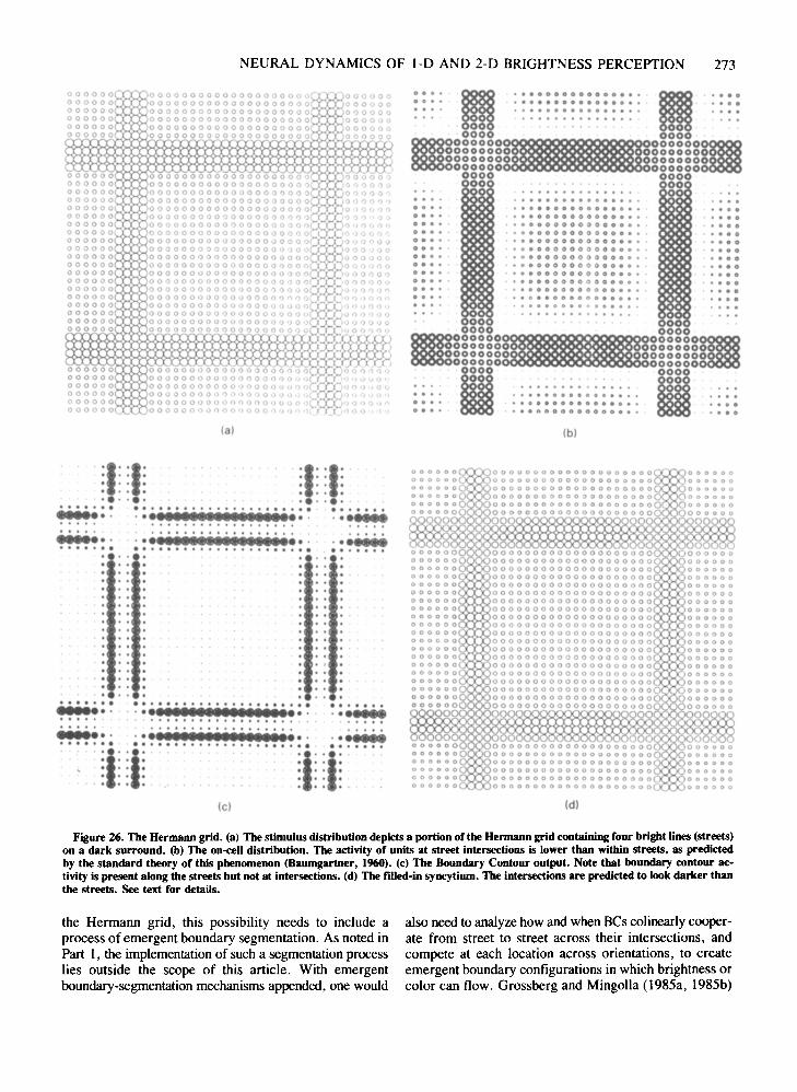
NEURAL DYNAMICS OF 1-0 AND 2-D BRIGHTNESS PERCEPTION 273
• • 0.00
I> 0 0 0
I> 0 0 0
o 000
o 000I> 0 00
o 000• 0 0 0I> 0 0 0
• 0 0
• • 0
.0000000000000
0000000000000.
0000000000000.'000000000000000
0000000000000000000000000000000000000000000000
01> 00000000000000 I>
000000000000000000000000000000000000000000000000
0000000000000000000000000000
0000000<>0000
o ••00 •o 0 0 I>
0.0 •
000 0(01) I>
000 0
00 0 •
o 0 0 I>
o 0 0 0
o ••o ••·
00 00·0000 0000
lIoooo°lmlli oOOOOOIlggggggg gggggggo00000 0000000·.. lIoggo
.... :. : : , . :. . . 1I088g ...00.000000000110
000. 00000000000000 '00
000. aoooOOOOOOOOOO 000
000 •.•• '.00000000000.' .•••• 000'. . ..000000000 •• 0.. . .'00
'0 "00000000' ••
• 00 . . : : : : : : : : : : . . 00.· . .. 0000 .. ..' ... . 0000· .. '.
110 0 0 0 0 0 _ 0 0 0 0 0 0110000000 00000000og~~~~go gg~~~~go
0000 . . . . 0000 .00 00
000000000000000000000000000000000000
I
00000'-:;OOQO')O
o o 0 00 oo o 0 0 I) I)
0') 0 (; () 0I) 'J () '\ o 'J
0') 0 (j o r-,
~I ,~ ~~ ~ ~ ~~ ~o 0 0 -» 0 0000 o 0 0000r)00
:::~~~Z~ZS;~;~ ~~ ~ ~ ~;]0 () I) 0 o ,)~0()f) o ,) ()
~<~~~~~~~en
M )J
00000000000000000000OOOOQOOOOoooooonooo,)00000000000000000000oooooa00000')0(}O.)OOL)r)0000000000000000000')00000noonOQr)OOO,'r}0 r \ r )
000000000000000000000000000000000000000000000000000000000000000000000000000000000000000000000000000000000000000000000000
0000000000000000000000000000000000000000000000000000000000000000000000000000000000000000000000000000000000000000000000000000000000000000000°800000000000000000000
OOOOOOOOOOOOOOOOOOOOi~(00000000000000000000000000000000000000000000000000000000000000000000000000000000000 0000000000000 0 o 0 o(000000000000000000000000000000000000000000000000000000000000OQOOOOOOOOQOOOQOQOQl)0000000000000000000')0000000000000000(1000
OOOC00000000000000000000000000000000
000000000000000000000000000000000000000000000000000000000000000000000000000000000000000000000000oaoooo000000000000000000
000000000000000000000000000000000000
(a) (b)
::1: :1: :1: :1:.. .. . . .. ... .. . . .. ... ' '.. ..' ' .......:~ ~:.iiiiiiiiiiiiiiii.:~ ~:.....
• •••• 4 • •••••• • • • • • • ••••
• • • 4 • • •••••• f ••••••••••..... ' . . . ....a a • • •• • • •••• a • • • • • • • • • • • • • • • • • ••••••... ... ...
••• ••• ••••••..... :~ ~:.iiiiiiiiiiiiiiii.:~ ~:.....• •••• t ••••••••• t • • • • • ••••
• •••• t ••••••• t ••••
..... . . • .......lIlIn••••• • . . ......••••••• •••••••••••• t.t •••• oII •••••••••••-:1::1·: :1::1·:· .. . . .. .
• •• • • oil. •· .. . . .. .
0000 0 o~o 0 0 0 0 0 0 0 0000000000 0 o~o 0 0 000000000 00000000000000000000 0000000000000 00000000000000000000 00000000000000 0000000000000000000000 00000000000000 0000000000000000000000 00000000000000 0000000000000000000000 0000000
ffgO~0~0~0~088:00000 0000008888833000 § 0 000 8888888
0000000 0000000000000000000000 00000000000000 0000000000000000000000 00000000000000 000000000000000000000 0000000000000 00000000000000000000 000000000000 00000000000000000000 000000000000 00000000000000000000 000000000000 00000000000000000000 000000000000 00000000000000000000 000000000000 00000000000000000000 000000000000 00000000000000000000 000000000000 00000000000000000000 000000oooeoo 00000000000000000000 000000000000 00000000000000000000 000000000000 00000000000000000000 000000000000 00000000000000000000 000000000000 00000000000000000000 000000000000 00000000000000000000 0000000000000 000000000000000000000 00000000000000 0000000000000000000000 0000000
~§§_§§§88882M~1188~000§8888880000000 00000000000000000000°9°0000000000000 0000000000000000000000 00000000000000 0000000000000000000000 00000000000000 00000000000000000000 0000000000000 00000000000000000000 000000000000 00000000000000000000 000000
(c) (d)
Figure 26. The Hermann grid. (a) The stimulus distribution depicts a portion of the Hermann grid containing four bright lines (streets)on a dark surround. (b) The on-eell distribution. The activity of units at street intersections is lower than within streets, as predictedby the standard theory of this phenomenon (Baumgartner, 1960). (c) The Boundary Contour output. Note that boundary contour activity is present along the streets but not at intersections. (d) The filled-in syncytium. The intersections are predicted to look darker thanthe streets. See text for details.
the Hermann grid, this possibility needs to include aprocess of emergent boundary segmentation, As noted inPart I, the implementation of such a segmentation processlies outside the scope of this article, With emergentboundary-segmentation mechanisms appended, one would
also need to analyze how and when BCs colinearly cooperate from street to street across their intersections, andcompete at each location across orientations, to createemergent boundary configurations in which brightness orcolor can flow. Grossberg and Mingolla (1985a, 1985b)
274 GROSSBERG AND TODOROVIC
have analyzed a number of achromatic and chromatic percepts that are strongly influenced by such emergent boundary segmentations.
PART 6DISCUSSION
The computer implementation of the model describedin this paper has a limited domain of application since itdeals only with monocular achromatic brightness effects.Extensions into the chromatic and binocular domains havebeen described in Grossberg (1987a, 1987b). Brightnesscan also be influenced by emergent segmentations that arenot directly induced by image contrasts, as in Kanizsa'sillusory triangle, the Ehrenstein illusion, and neon colorspreading effects. These and related grouping and segmentation effects have been discussed by Grossberg andMingolla (1985a, 1985b). Their implementation includesa version of the BC System in which emergent segmentations can be generated through lateral interactions between oriented channels. Such interactions may playa rolein the orientation-sensitive brightness effects reported byMcCourt (1982), Sagi and Hochstein (1985), and White(1979). The implementation in this paper also omits possible effects of multiple-scale processing, as the receptive fields of all units within a network were assumed tohave a single receptive field size. Units of multiple sizesmay be involved in the explanation ofclassical brightnessassimilation (Helson, 1963). Grossberg and Mingolla(1987) have studied the role of multiple scales in the perception of 3-D smoothly curved and shaded objects. Anumber of depth-related effects, such as in phenomenaof transparency (Metelli, 1974) and proximity-luminancecovariance (Dosher, Sperling, & Wurst, 1986) have beendiscussed by Grossberg (1987a, 1987b). The model in itscurrent form also does not treat the temporal variationsof brightness due to image motion (Cavanagh & Anstis,1986; Todorovic, 1983, 1987) or stabilization (Krauskopf,1963; Pritchard, 1961; Yarbus, 1967). Finally, the application of the model to natural noisy images has yet tobe accomplished.
In sum, the system described in this paper does not attempt to explain the complete gamut of brightnessphenomena. These limitations are not, however, insurmountable obstacles; rather, they point to natural extensions of the model, many of which have been discussedand implemented in related work. However, even theprocessing of brightness in monocular, achromatic, static,noise-free images is full of surprising complexities. Onlya model capable of handling these basic phenomena canbe a foundation upon which still more complex effectscan be explained.
Surprisingly little computationally oriented work hasbeen devoted to these fundamental aspects of visual perception. Several contemporary algorithms were influencedby Land's seminal work (Blake, 1985; Frisby, 1979;Hom, 1974). Other computational models have providedalternative approaches to the analysis of filling-in (Arend
& Goldstein, 1987; Hamada, 1984). Our model has beenused to simulate a much larger set of brightness data, andincludes mechanistic explanations of classical longstanding phenomena described in every review of brightness processing, recently discovered but unexplained data,and predictions of yet untested phenomena, includingpredictions of testable patterns of physiological activation.
The direct measurement of spatial distributions of activity in real neural networks is still hampered by considerable technical difficulties. Recently, a number ofprocedures have been developed to enable the visualization of the spatial patterning of activation across largenumbers of neurons to a given stimulus (Blasdel &Salama, 1986; Fox et al., 1986; Grinvald, Leike, Frostig,Gilbert, & Wiesel, 1986; Nothdurft & Lee, 1982). Thesenew techniques offer exciting possibilities for the studyof integrating brain functions. Our computer simulationsillustrate that these spatial patterns can be qualitativelydifferent in response to the same stimulus at differentlevels of functional organization, and predict the types ofactivation patterns that should be elicited by images thatare easily acquired and used in the laboratory. Of particular importance to brightness theory will be the discovery and mechanistic characterization of the cortical fillingin domains whose properties have been so essential to thesuccess of our computer simulations of brightnesspercepts.
REFERENCES
AREND, L. E. (1973). Spatial differential and integral operations in human vision: Implication of stabilized retinal image fading. Psychological Review, SO, 374-395.
AREND, L. E., BUEHLER, J. N., & LocKHEAD, G. R. (1971). Difference information in brightness perception. Perception & Psychophysics, 9, 367-370.
AREND, L. E., & GOLDSTEIN, R. E. (1987). Lightness models, gradientillusions, and curl. Perception & Psychophysics, 42, 65-80.
AREND, L. E., & REEVES, A. (1986). Simultaneous color constancy.Journal of the Optical Society of America, AJ, 1743-1751.
BAUMGARTNER, G. (1960). Indirekte Grossenbestimmung der receptiven Felder der Retina beim Menschen mittels der HermannschenGittertiiuschung (Abstract). PfTiigers Archifiir die GesamzePhysiologie,272, 21-22.
BECK, J. (1966a). Effect of orientation and of shape similarity on perceptual grouping. Perception & Psychophysics, 1, 300-302.
BECK, J. (1966b). Perceptual grouping produced by changes in orientation and shape. Science, 154, 528-540.
BERMAN, P. W., & LEIBOWITZ, H. W. (1965). Some effects of contouron simultaneous brightness contrast. Journal ofExperimental Psychology, 69, 251-256.
BLAKE, A. (1985). Boundary conditions for lightness computation inMondrian world. Computer Vision, Graphics. & Image Processing,14, 314-327.
BLASDEL, G. G., & SALAMA, G. (1986). Voltage-sensitive dyes reveala modular organization in monkey striate cortex. Nature, 321, 579-585.
BRAITENBERG, V., & BRAITENBERG, C. (1979). Geometry of orientation columns ill the visual cortex. Biological Cybernetics, 33, 179-186.
BRIDGEMAN, B. (1983). Isomorphism is where you find it. Behavioral& Brain Sciences, 6, 658-659.
CAVANAGH, P., & ANSTIS, S. M. (1986). Brightness shift in driftingramp gratings isolates a transient mechanism. Vision Research, 26,899-908.
COHEN, M. A., & GROSSBERG, S. (1984). Neural dynamics of bright-
NEURAL DYNAMICS OF I-D AND 2-D BRIGHTNESS PERCEPTION 275
ness perception: Features, boundaries, diffusion, and resonance. Perception & Psychophysics, 36, 428-456.
CORNSWEET, T. N. (1970). Visual perception. New York: AcademicPress.
DAVIDSON, M., & WHITESIDE, J. A. (1971). Human brightness perception near sharp contours. Journal ofthe Optical Society ofAmerica,61, 530-536.
DEVALOIS, R. L., ALBRECHT, D. G., & THORELL, L. G. (1982). Spatial frequency selectivity of cells in macaque visual cortex. VisionResearch, 22, 545-559.
DOSHER, B. A., SPERUNG, G., & WURST, S. (1986). Tradeoffs betweenstereopsis and proximity luminance covariance as determinants of perceived 3-D structure. Vision Research, 26, 973-979.
ENROTH-CUGELL, C., & ROBSON, J. G. (1966). The contrast sensitivity of retinal ganglion cells of the cat. Journal of Physiology, 187,517-552.
ENROTH-CUGELL, c., & ROBSON, J. G. (1984). Functional characteristicsand diversity of cat retinal ganglion cells. Investigative Ophthalmology & Visual Science, 25, 250-267.
ESCHER, M. C. (1961). The graphic work of M. C. Escher. London:Oldburne.
FECHNER, G. T. (1889). Elemente der Psychophysik (2nd ed.). Leipzig: Breitkopf & Hartel.
FOSTER, D. H. (1983). Experimental test of a network theory of vision. Behavioral & Brain Sciences, 6, 664-665.
Fox, P. T., MINTUN, M. A., RAICHLE, M. E., MIEZIN, F. M.,ALLMAN, J. M., & VANESSEN, D. C. (1986). Mapping human visualcortex with positron emission tomography. Nature, 323, 806-809.
FRISBY, J. P. (1979). Seeing: Illlusion, brain, and mind. Oxford: Oxford University Press.
FRY, G. A. (1948). Mechanisms subserving simultaneous brightnesscontrast. American Journal ofOptometry and Archives ofthe American Academy of Optometry, 25,162-178.
GERRITS, H. J. M., & VENDRICK, A. J. H. (1970). Simultaneous contrast, filling-in process and information processing in man's visualsystem. Experimental Brain Research, 11, 411-430.
GOURAS, P., & KRUGER, J. (1979). Responses of cells in foveal visualcortex of the monkey to pure color contrast. Journal ofNeurophysiology, 42, 850-860.
GRINVAW, A., LEIKE, E., FROsnG, R. D., GILBERT, C. D., & WIESEL,T. N. (1986). Functional architecture of cortex revealed by opticalimaging of intrinsic signals. Nature, 324, 361-364.
GROSSBERG, S. (1983). The quantized geometry of visual space: Thecoherent computation of depth, form, and lightness. Behavioral &Brain Sciences, 6, 625-692.
GROSSBERG, S. (1987a). Cortical dynamics of three-dimensional form,color, and brightness perception: I. Monocular theory. Perception &Psychophysics, 41, 87-116.
GROSSBERG, S. (1987b). Cortical dynamics of three-dimensional form,color, and brightness perception: n. Binocular theory. Perception &Psychophysics, 41, 117-158.
GROSSBERG, S., & MINGOLLA, E. (1985a). Neural dynamics of formperception: Boundary completion, illusory figures, and neon colorspreading. Psychological Review, 92, 173-211.
GROSSBERG, S., & MINGOLLA, E. (1985b). Neural dynamics ofperceptuaIgrouping: Textures, boundaries, and emergent segmentations. Perception & Psychophysics, 38, 141-171.
GROSSBERG, S., & MINGOLLA, E. (1987). Neural dynamics of surfaceperception: Boundary webs, iIIuminants, and shape-from-shading.Computer Vision, Graphics, & Image Processing, 37, 116-165.
GROSSBERG, S., & MINGOLLA, E. (1988). The role of illusory contoursin visual segmentation. In S. Petry & G. Meyer (Eds.), Theperception of illusory contours. New York: Springer-Verlag.
GROWNEY, R. L., & NERI, D. F. (1986). The appearance of the Cornsweet illusion: Measures of perceived contrast and evenness of brightness. Perception & Psychophysics, 39, 81-86.
HAMADA, J. (1984). A multistage model for border contrast. Biological Cybernetics, 51, 65-70.
HEGGE LUND, P. (l98Ia). Receptive field organisation of simple cellsin cat striate cortex. Experimental Brain Research, 42, 89-98.
HEGGE LUND, P. (1981b). Receptive field organisation of complex cellsin cat striate cortex. Experimental Brain Research, 42, 99-107.
HEGGELUND, P. (1985). Quantitative studies of enhancement and suppression zones in the receptive field of simple cells in cat striate cortex. Journal of Physiology, 373, 293-310.
HEINEMANN, E. G. (1972). Simultaneous brightness induction. InD. Jameson & L. M. Hurvich (Eds.), Handbook ofsensory physiology: Vol. Vlll4. Visualpsychophysics (pp. 146-169). Berlin: SpringerVerlag.
HELSON, H. (1963). Studies of anomalous contrast and assimilation.Journal of the Optical Society of America, 53, 179-184.
HESS, C., & PRETORI, H. (1894). Messende Untersuchungen uber dieGesetzmassigkeit des simultanen Helligkeitscontrastes. Albrecht v.Graefes Archiv fiir Ophthalmologie, 40, 1-24.
HORN, B. K. P. (1974). Determining lightness from an image. Computer Graphics & Image Processing, 3, 277-299.
HUBEL, D. H., & WIESEL, T. N. (1962). Receptive fields, binocularinteraction and functional architecture in the eat's visual cortex. Journalof Physiology, 160, 106-154.
HUBEL, D. H., & WIESEL, T. N. (1968). Receptive fields and functional architecture of monkey striate cortex. Journal ofPhysiology,195, 215-243.
HURVICH, L. M. (1981). Color vision. Sunderland, MA: Sinauer.JULESZ, B. (1971). Foundations of cyclopean perception. Chicago:
University of Chicago Press.KANIZSA, G., & MINGUZZI, G. F. (1986). An anomalous brightness
differentiation. Perception, 15, 223-226.KATO, H., BISHOP, P.O., & ORBAN, G. A. (1978). Hypercomplex and
simple/complex cell classifications in cat striate cortex. Journal ofNeurophysiology, 41, 1071-1095.
KATZ, D. (1935). The world ofcolour. London: Kegan Paul, Trench,Trubner.
KOFFKA, K. (1935). Principles ofGestalt psychology. New York: Harcourt & Brace.
KRAUSKOPF, J. (1963). Effect ofretinal image stabilization on the appearance of heterochromatic targets. Journal of the Optical Societyof America, 53, 741-744.
LAMING, D. (1983). On the need for discipline in the construction ofpsychological theories. Behavioral & Brain Sciences, 6, 669-670.
LAND, E. (1977). The retinex theory of color vision. Scientific American, 237, 108-128.
LAND, E. (1986). Recent advances in retinex theory. Vision Research,26, 7-21.
LAND, E. & McCANN, J. J. (1971). Lightness and retinex theory. Journalof the Optical Society of America, 61, 1-11.
MCCOURT, M. E. (1982). A spatial frequency dependent gratinginduction effect. Vision Research, 22, 119-134.
METELU, F. (1974). The perception oftransparency. Scientific American, 230, 90-98.
METZGER, W. (1930). Optische Untersuchungen am Ganzfeld: n. ZurPhiinomenologie des homogenen Ganzfeldes. Psychologische Forschung, 13, 6-29.
NIELSEN, D. E. (1985). Retinocortical wiring of the simple cells of thevisual cortex. In D. Rose & V. G. Dobson (Eds.), Models ofthe visualcortex. New York: Wiley.
NOTHDURFT, H. C., & LEE, B. B. (1982). Responses to colored patterns in the macaque lateral geniculate nucleus: Pattern processingin single neurons. Experimental Brain Research, 48, 43-54.
PENROSE, L. S., & PENROSE, R. (1958). Impossible objects: A specialtype of visual illusion. British Journal of Psychology, 49, 31-33.
PICCOUNO, M., NEYTON, J., & GERSCHENFELD, H. M. (1984). Decreaseof gap junction permeability induced by dopamine and cyclic adenosine 3':5'-monophosphate in horizontal cells of turtle retina. Journalof Neuroscience, 4, 2477-2488.
PRITCHARD, R. M. (1961). Stabilized images on the retina. ScientificAmerican, 204, 72-78.
276 GROSSBERG AND TODOROVIC
and
The duality between on-cell and off-cell receptive fields wasachieved by setting
The output signal from Level 2 is the nonnegative, or rectified,part of Xij:
(A2)
(A3)
(A6)
(A9)
(A7)
(A8)
1:cc.;(p,q)
E IpqEpqih
(p,q)
Xij =
Cpqi} Cexp{ -a-'log2[(p-i)' + (q-j)']) (A4)
where
and
and
ddtXij = -Axij + (B-Xij)Cij - (xij+D)Eij, (AI)
where Cij (E i) is the total excitatory (inhibitory) input to Xij'Each input Cij and Eij is a discrete convolution with Gaussiankernel of the inputs Ipq:
Level 2The activity x., of a Level 2 on-cell at position (i,j) of the
lattice obeys a membrane equation
1 and 9. To compute the spatial convolutions of Level 2 cellswithout causing spurious edge effects at the extremities of theluminance profile, the luminance values at the extremities werecontinued outward as far as necessary.
The denominator term normalizes the activity Xij'The off-cell potential xij at position (i,j) also obeys a mem
brane equation with an equilibrium value of the same form
E (p,q) (BCpqij - DEpqij)Ipq
A +E(p,q)(Cpqij+Epqij)Ipq
Epqij = E exp{ -{3-'log2[(p-i)' + (q-jY]). (A5)
Thus, the influence exerted on the Level 2 potential Xijby inputI pq diminishes with increasing distance between the two corresponding locations. The decrease is isotropic, inducing thecircular shape of the receptive fields. To achieve an on-centeroff-surround anatomy, coefficient C of the excitatory kernel inEquation A4 is chosen larger than coefficient E of the inhibitory kernel in Equation A5, but a, the radius of the excitatoryspread at half strength in Equation A4, is chosen smaller than{3, its inhibitory counterpart in Equation A5. In the simulations,this equation is solved at equilibrium. Then (dldt)Xij = 0, so that
E (p,q)(BCpqij - DEpqij)IpqXij == .
A +E(p,q)(Cpqij+Epqi})Ipq
The equations underlying the model are based on and are anextension of work by Grossberg (1983), Cohen and Grossberg(1984), and Grossberg and Mingolla (1985b, 1987a). The exposition follows the description of levels in Figure 2. Only the2-D versions of the equations are presented. The I-D forms canbe derived by straightforward simplifications. The 2-D simulations were performed either on a 16x 16 lattice of units (the yinyang square), a 30x30 lattice (simulations in Part 5-The COCEwith and without ... and Percept of an impossible staircase ... ),or a 40 x 40 lattice (all other simulations). The one-dimensionalsimulations involve 256 units.
APPENDIX
RATLIFF, F. (1965). Mach bands: Quantitative studies on neural networks in the retina. New York: Holden-Day.
RATLIFF, F., & HARTLINE, H. U. (1959). The response of limulus optic nerve fibers to patterns of illumination on the receptor mosaic.Journal of General Physiology, 42,1241-1255.
RATLIFF, F., & SIROVICH, L. (1978). Equivalence classes of visualstimuli. Vision Research, 18, 845-851.
SAGI, D., & HOCHSTEIN, S. (1985). Lateral inhibition between spatiallyadjacent spatial-frequency channels? Perception & Psychophysics, 37,315-322.
SCHILLER, P. H., FINLAY, B. L., & VOLMAN, S. F. (1976). Quantitative studies of single-cell properties in monkey striate cortex: 1.Spatiotemporal organization of receptive fields. Journal ofNeurophysi010gy,39, 1288-1319.
SEKULER, R. (1974). Spatial vision. In P. H. Mussen & M. R. Rosenzweig (Eds.), Annual Review of Psychology. Palo Alto: AnnualReviews.
SHAPLEY, R. (1986). The importance of contrast for the activity of single neurons, the VEP and perception. Vision Research, 26, 45-61.
SHAPLEY, R., & REID, R. C. (1986). Contrast and assimilation in theperception of brightness. Proceedings of the National Academy ofSciences USA, 82, 5983-5986.
SILLlTO, A. M. (1984). Functional considerations of the operation ofGABAergic inhibitory processes in the visual cortex. In A. Peters& E. G. Jones (Eds.), Cerebral cortex (Vol. 2A). New York: Plenum Press.
SPITZER, H., & HOCHSTEIN, S. (1985). A complex-cell receptive fieldmodel. Journal of Neurophysiology, 53, 1266-1286.
TANAKA, M., LEE, B. 8., & CREUTZFELDT, O. D. (1983). Spectral tuning and contour representation in area 17 of the awake monkey. In1. D. Mollon & L. T. Sharpe (Eds.), Colour vision. New York: Academic Press.
TODOROVIC, D. (1983). Brightness perception and the Craik-O'BrienComsweet effect. Unpublished master's thesis, University of Connecticut, Storrs.
TODOROVIC, D. (1987). The Craik-O'Brien-Cornsweet effect: New varieties and their theoretical implications. Perception & Psychophysics,42, 545-560.
WALLACH, H, (1948). Brightness constancy and the nature of achromatic colors. Journal of Experimental Psychology, 38, 310-324.
WALLACH, H. (1976). On perception. New York: Quadrangle.WALLS, G. (1954). The filling-in process. American Journal ofOptom
etry, 31, 329-340.WHITE,M, (1979). A new effect of pattern on perceived lightness. Per
ception, 8, 413-416.YARBUS, A. L. (1967). Eye movements and vision. New York: Plenum
Press.YUND,E. W., & ARMINGTON, J. C. (1975). Color and brightness con
trast effects as a function of spatial variables. Vision Research, 15,917-930.
LevellWe denote by Iij the value of the stimulus input at position
(i,j) in the lattice. In all simulations these values varied between
(A10)
Level 3The potential Yijk of the cell centered at position (i,j) with
NEURAL DYNAMICS OF I-D AND 2-D BRIGHTNESS PERCEPTION 277
Level 6(AI2) Each potential Sij at position (i,j) of the syncytium obeys a
nonlinear diffusion equation
orientation k on the hour code in Figure 7 obeys an additiveequation
LevelSA Level 5 signal Zij at position (i,j) is the sum of output sig
nals from all Level 4 units at that position; viz.,ddt Yijk = -Yijk + E Xp.F~:L
(p,q)
which is computed at equilibrium
Yijk = E xp.F~:lj(p,q)
(All)z; = EZijk.
k
(A21)
in all our simulations. To generate an oriented kernel F~:lj assimply as possible, let F~:t be the difference of an isotropickernel Gp•ij centered at (i,j) and another isotropic kernel H~:lj
whose center (i+m.,j+nk ) is shifted from (i,j) as follows:
(A23)s
Pp q ij = .1+ f(Zp.+Zij)
The set Nijof locations comprises only the lattice nearest neighbors of (i,j):
Nij={(i,j-l), (i-l,j), (i+l,j), (i,j+l)}. (A24)
ddt Sij = -MSij+ E (SP.-Sij)PP.ij+Xj. (A22)
(p,q) EN,;
The diffusion coefficients that regulate the magnitude of crossinfluence oflocation (i,j) with location (p,q) depend on the BCsignals ZP' and Zij as follows:
(AI3)
(A 14)Gp • ij = exp{ -'Y-2[( p - i )2+ (q _ j )2]}
where
with
and
An output signal Zijk is generated from Level 4 to Level 5 ifthe activity Zijk exceeds the threshold L:
In the 2-D simulations, the number K of hour codes is 12,whereas for the I-D simulations it is 2.
The output signal from Level 3 to Level 4 is the nonnegative, or rectified, part of Yijk, namely
Level 4Each Level 4 potential Zijk with position (i,j) and orientation
k is made sensitive to orientation but insensitive to direction ofcontrast by summing the output signals from the appropriate pairof Level 3 units with opposite contrast sensitivities; viz.,
(A25)
At lattice edges and comers, this set is reduced to the set ofexisting neighbors. According to Equation A22, each potentialSij is activated by the on-cell output signal X j and thereuponengages in passive decay (term -MSi) and diffusive filling-inwith its four nearest neighbors to the degree permitted by thediffusion coefficients PP"j. At equilibrium, each Sij is computedas the solution of a set of simultaneous equations
X'j+ E(P.•IEN"Sp.Pp.ijS'j = ----=----
M+E(p"IEN"Pp,'j
which is compared with properties of the brightness percept.In all simulations, the following parameter values were used:
A = 1, B = 90, D = 60, l' = 1. Due to differences in dimensionality and scale, several parameters were given different valuesacross sets of simulations. All 2-D simulations shared the following parameters: C=18, M= 1, a=.25, f= 1. The yin-yangsquare (16 X 16) simulations used E= 1, {3=2, 0= 100, L= 15.All other 2-D (30x 30 and 40 X 40) simulations usedE=.5, {3=3,0=300, L=IO. AlII-D simulations used C=4, M=IO, a=l,f=I00, E=.5, {3=8, 0 =100,000, L=5.
Finally, to illustrate the effects of parameter changes, the following values were different from the ones listed above. InFigure 00,1'=3. In Figures 16c and 16d, f=l,ooo. In Figures 16a and 16b, the BC signal Z, was transformed throughthe sigmoid function IOZ~(1 +ZD-l.
(AI6)
(AI7)
(AI8)
(AI9)
(A20)
27rkm; = sinK
211"knk = cosK .
Zijk = Y,jk +Yij[k+(K /2) J.
and
(Manuscript received April 8, 1987;revision accepted for publication September 8, 1987.)