Embed Size (px)
Citation preview
Perception & Psychophysics1984, 36 (5), 428-456
Neural dynamics of brightness perception:Features, boundaries, diffusion, and resonance
MICHAEL A. COHEN and STEPHEN GROSSBERGBoston University, Boston, Massachusetts
A real-time visual processing theory is used to unify the explanation of monocular and binocularbrightness data. This theory describes adaptive processes which overcome limitations of the visualuptake process to synthesize informative visual representations of the external world. The brightness data include versions ofthe Craik-O'Brien-Cornsweet effect and its exceptions, Bergstrom'sdemonstrations comparing the brightnesses of smoothly modulated and step-like luminance profiles, Hamada's demonstrations of nonclassical differences between the perception of luminancedecrements and increments, Fechner's paradox, binocular brightness averaging, binocular brightness summation, binocular rivalry, and fading of stabilized images and ganzfelds. Familiar concepts such as spatial frequency analysis, Mach bands, and edge contrast are relevant but insufficient to explain the totality of these data. Two parallel contour-sensitive processes interact togenerate the theory's brightness, color, and form explanations. A boundary-contour process issensitive to the orientation and amount of contrast but not to the direction of contrast in scenicedges. It generates contours that form the boundaries of monocular perceptual domains. The spatialpatterning of these contours is sensitive to the global configuration of scenic elements. A featurecontour process is insensitive to the orientation of contrast, but is sensitive to both the amountof contrast and to the direction of contrast in scenic edges. It triggers a diffusive filling-in reaction of featural quality within perceptual domains whose boundaries are dynamically definedby boundary contours. The boundary-contour system is hypothesized to include the hypercolumnsin visual striate cortex. The feature-contour system is hypothesized to include the blobs in visualstriate cortex. These preprocessed monocular activity patterns enter consciousness in the theoryvia a process of resonant binocular matching that is capable of selectively lifting whole monocular patterns into a binocular representation of form-and-color-in-depth. This binocular processis hypothesized to occur in area V4 of the visual pre striate cortex.
(1) Paradoxical Percepts as Probes ofAdaptive Processes
This article describes quantitative simulations ofmonocular and binocular brightness data to illustrate andsupport a real-time perceptual processing theory. This theory introduces new concepts and mechanisms concerning how human observers achieve informative perceptualrepresentations of the external world that overcome limitations of the sensory uptake process, notably of how distributed patterns of locally ambiguous visual features canbe used to generate unambiguous global percepts.
For example, light passes through retinal veins beforeit reaches retinal photoreceptors. Human observers do notperceive their retinal veins due to the action of mechanisms that attenuate the perception of images that are stabilized with respect to the retina. Mechanisms capable of
M. A. Cohen was supported in part by the National Science Foundation (NSF-IST-80-00257) and the Office of Naval Research (ONRNOOOI4-83-K0337). S. Grossberg was supported in part by the Air ForceOffice of Scientific Research (AFOSR 82-0148) and the Office of NavalResearch (ONR-NOOOI4-83-K0337). We thank Cynthia Suchta for hervaluable assistance in the preparation of the manuscript and illustrations.
The authors' mailing address is: Center for Adaptive Systems, BostonUniversity, III Cummington Street, Boston, MA 02215.
generating this adaptive property of visual percepts canalso generate paradoxical percepts, as during the perception of stabilized images or ganzfelds (Pritchard, 1961;Pritchard, Heron, & Hebb, 1960; Riggs, Ratliff, J. C.Cornsweet, & T. N. Cornsweet, 1953; Yarbus, 1967).Once such paradoxical percepts are traced to an adaptiveperceptual process, they can be used as probes to discoverthe rules governing this process. This type of approachhas been used throughout the research program on perception (Carpenter & Grossberg, 1981; Cohen & Grossberg, 1984; Grossberg, 1980, 1982a, 1983a, 1983b;Grossberg & Mingolla, 1985, in press) of which this workforms a part.
Suppressing the perception of stabilized veins is insufficient to generate an adequate percept. The images thatreach the retina can be occluded and segmented by theveins in several places. Somehow, broken retinal contoursneed to be completed, and occluded retinal color andbrightness signals need to be filled in. Holes in the retina, such as the blind spot or certain scotomas, are alsonot visually perceived (Gerrits, de Haan, & Vendrick,1966; Gerrits & Timmermann, 1969; Gerrits & Vendrick,1970) due to some sort of filling-in process. These completed boundaries and filled-in colors are illusory percepts,
Copyright 1985 Psychonomic Society, Inc. 428

NEURAL DYNAMICS OF BRIGHTNESS PERCEPTION 429
albeit illusory percepts with an important adaptive value.The large literature on illusory figures and filling in canthus be used as probes of this adaptive process (Arend,Buehler, & Lockhead, 1971; Day, 1983; Gellatly, 1980;Kanizsa, 1974; Kennedy, 1978, 1979, 1981; Parks, 1980;Parks & Marks, 1983; Petry, Harbeck, Conway, &Levey, 1983; Redies & Spillmann, 1981; van Tuijl, 1975;van Tuijl & de Weert, 1979; Yarbus, 1967). The brightness simulations that we report herein illustrate our theory's proposal for how real and illusory boundaries arecompleted and features are filled in.
Retinal veins and the blind spot are not the only blemishes of the retinal image. The luminances that reach theretina confound inhomogeneous lighting conditions withinvariant object reflectances. Workers since the time ofHelmholtz (Helmholt, 1962) have realized that the brainsomehow "discounts the illuminant" to generate colorand brightness percepts that are more accurate than theretinal data. Land (1977) has shown, for example, thatthe perceived colors within a picture constructed fromoverlapping colored patches are determined by the relative contrasts at the edges between the patches. The luminances within the patches are somehow discounted.These data also point to the existence of a filling-inprocess. Were it not possible to fill in colors to replacethe discounted illuminants, we would perceive a worldof boundaries rather than one of extended forms.
Since edges are used to generate filled-in percepts, anadequate perceptual theory must define edges in a waythat can accomplish this goal. We suggest that the edgecomputations whereby boundaries are completed are fundamentally different-in particular, they obey differentrules-from the edge computations leading to color andbrightness signals. We claim that both types of edges arecomputed in parallel before being recombined to generate filled-in percepts. Our theory hereby suggests that thefundamental question "What is an edge, perceptuallyspeaking?" has not adequately been answered by previous theories. One consequence of our answer is a physical explanation and generalization of the retinex theory(Grossberg, 1985), which Land (1977) has developedto explain his experiments.
The present article further supports this conception ofhow edges are computed by qualitatively explaining, andquantitatively simulating on the computer, such paradoxical brightness data as versions of the Craik-O'BrienCornsweet effect (Arend et al., 1971; Cornsweet, 1970;O'Brien, 1958) and its exceptions (Coren, 1983; Heggelund & Krekling, 1976; van den Brink & Keemink,1976; Todorovic, 1983), the Bergstrom demonstrationscomparing the brightnesses of smoothly modulated andstep-like luminance profiles (Bergstrom, 1966, 1967a,1967b), and the demonstrations of Hamada (1980) showing nonclassical differences between the perception of luminance decrements and increments. These percepts canall be seen with one eye. Our theory links thesephenomena to the visual mechanisms that are capable of
preventing perception of retinal veins and the blind spot,and that fill in over discounted illuminants, which alsooperate when only one eye is open.
Due to the action of binocular visual mechanisms thatgenerate a self-consistent percept of depthful forms, somevisual images that can be monocularly perceived may notbe perceived during binocular viewing conditions. Binocular rivalry provides a classical example of this fact (Blake& Fox, 1974; Cogan, 1982; Kaufman, 1974; Kulikowski,1978). To support the theory's conception of how depthful form percepts are generated (Cohen & Grossberg,1984; Grossberg, 1983a, 1983b), we suggest explanationsand provide simulations of data concerning inherentlybinocular brightness interactions. These data includeresults on Fechner's paradox, binocular brightness summation, binocular brightness averaging, and binocularrivalry (Blake, Sloane, & Fox, 1981; Cogan, 1982;Cogan, Silverman, & Sekuler, 1982; Curtis & Rule, 1980;Legge & Rubin, 1981; Levelt, 1965).
These simulations do not, of course, begin to exhaustthe richness of the perceptual literature. They are meantto be illustrative, rather than exhaustive, of a perceptualtheory that is still undergoing development. On the otherhand, this incomplete theory already reveals the perhapseven more serious incompletenessof rival theories by suggesting concepts and explaining data that are outside therange of these rival theories. The article also illustratesthe theory's burgeoning capacity to integrate the explanation of perceptual data by providing simulations of dataabout Fechner's paradox, binocular brightness averaging,binocular brightness summation, and binocular rivalry using the same model parameters that were established tosimulate disparity matching, filling-in, and figure-groundsynthesis (Cohen & Grossberg, 1984).
Although our theory was derived from perceptual dataand concepts, after it reached a certain state in its development, striking formal similarities with recent neurophysiological data could not fail to be noticed. Some of theserelationships are briefly summarized in Table 1 below.Although the perceptual theory can be understood withoutconsidering its neurophysiological interpretation, if oneis willing to pursue this interpretation, then the perceptual theory implies a narnber of neurophysiological andanatomical predictions. Such predictions enable yetanother data base to be used for the further developmentand possible disconfirmation of the theory.
A search through the neurophysiological literature hasrevealed that some of these predictions were already supported by known neural data, albeit data that took on newmeaning in the light of the perceptual theory. Not all ofthe predictions were known, however. In fact, two of itspredictionsabout the process of boundary completionhaverecently received experimental support from recordingsby von der Heydt, Peterhans, and Baumgartner (1984)on cells in area 18 of the monkey visual cortex. Neurophysiological interpretations and predictions of the theory are described in Grossberg and Mingolla (in press).

430 COHEN AND GROSSBERG
Due to the existence of this neural interpretation, we willtake the liberty of calling the formal nodes in our network"cells" throughout the article. The next sections summarize the concepts that we use to explain brightness data.
(2) The Boundary-Contour System and theFeature-Contour System
The theory asserts that two distinct types of edge, orcontour, computations are carried out within two parallelsystems. We call these systems the boundary-contour system and the feature-contour system. Boundary-contoursignals are used to synthesize the boundaries, whether"real"or "illusory," that the perceptual process generates. Feature-contour signals initiate the filling-inprocesses whereby brightnesses and colors spread untilthey either hit their first boundary contour or are attenuated due to their spatial spread. Boundary contours arenot, in themselves, visible. They gain visibility by restricting the filling-in that is triggered by feature-contoursignals.
These two systems obey different rules. The main rulescan be summarized as follows.
(3) Boundary Contours and BoundaryCompletion
The process whereby boundary contours are built upis initiated by the activation of oriented masks, or elongated receptive fields, at each position of perceptual space(Hubel & Wiesel, 1977). Our perceptual analysis leadsto the following hypotheses about how these masks activate their target cells, and about how these cells interactto generate boundary contours.
(a) Orientation and contrast. The output signals fromthe oriented masks are sensitive to the orientation and tothe amount of contrast, but not to the direction of contrast, at an edge of a visual scene. Thus, a vertical boundary contour can be activated by either a close-to-verticaldark-light edge or a close-to-verticallight-dark edge ata fixed scenic position. The process whereby two likeoriented masks that are sensitive to direction of contrastat the same perceptual location give rise to an output signal that is not sensitive to direction of contrast is designated by a plus sign in Figure lao
(b) Short-range competition. (i) The cells that reactto output signals due to like-oriented masks compete between nearby perceptual locations (Figure lb). Thus, amask of fixed orientation excites the like-oriented cellsat its location and inhibits the like-oriented cells at nearbylocations. In other words, an on-center off-surround organization of like-oriented cell interactions exists aroundeach perceptual location. (ii) The outputs from this competitive stage input to the next competitive stage. At thisstage, cells compete that represent perpendicular orientations at the same perceptual location (Figure lc). Thiscompetition defines a push-pull opponent process. If agiven orientation is inhibited, then its perpendicular orientation is disinhibited.
In all, a stage of competition between like orientationsat different, but nearby, positions is followed by a stage
~(a)
(d)
Figure 1. (a) Boundary-contour inputs are sensitive to the orientation and amount of contrast at a scenic edge, but not to its direction of contrast. (b) Like orientations compete at nearby perceptuallocations. (c) Different orientations compete at each perceptuallocation. (d) Once activated, aligned orientations can cooperateacross a larger visual domain to form real or illusory contours.
of competition between perpendicular orientations at thesame position.
(c) Long-range oriented cooperation and boundarycompletion. The outputs from the last competitive stageinput to a spatially long-range cooperative process thatis called the "boundary-completion" process. Outputs dueto like-oriented masks that are approximately alignedacross perceptual space can cooperate via this process tosynthesize an intervening boundary. The boundarycompletionprocess is capable of synthesizing global visualboundaries from local scenic contours (Grossberg & Mingolla, 1985, in press). Both "real" and "illusory" boundaries are assumed to be generated by this boundarycompletion process.
Two simple demonstrations of a boundary-completionprocess with properties a-c can be made as follows. InFigure 2a, four Pac-man figures are arranged at the vertices of an imaginary rectangle. It is a familiar fact thatan illusory Kanizsa (1974) square can be seen when allfour Pac-man figures are black against a white background. The same is true when two Pac-man figures areblack, the other two are white, and the background is gray,as in Figure 2b. The black Pac-man figures form darklight edges with respect to the gray background. The whitePac-man figures form light-dark edges with the gray background. The visibilityof illusory edges around the illusory

NEURAL DYNAMICS OF BRIGHTNESS PERCEPTION 431
....(a)
(b)Figure 2. <a) An illusory Kanizsa square is induced by four black
Pac-man fIgUreS. (b) An illusory square is induced by two black andtwo white Pac-man figures on a gray background. D1usorycontourscan thus join edges with opposite directions of contrast (The effectmay be weakened by the photographic reproduction process.)
square shows that a process exists that is capable ofcompleting contours between edges with opposite directionsof contrast. This contour-completion process is thus sensitive to amount of contrast but not to direction of contrast..
Another simple demonstration of these contourcompleting properties can be constructed as follows. Divide a square into two equal rectangles along an imaginary boundary. Color one rectangle a uniform shade ofgray. Color the other rectangle in shades of gray thatprogress from light to dark as one moves from end I ofthe rectangle to end 2 of the rectangle. Color end I alighter shade than the uniform gray of the other rectan-
gle, and color end 2 a darker shade than the uniform grayof the other rectangle. Then, as one moves from end Ito end 2, an intermediate gray region is passed whose luminance approximately equals that of the uniform rectangle. At end 1, a light-dark edge exists from the nonuniform rectangle to the uniform rectangle. At end 2, adark-light edge exists from the nonuniform rectangle tothe uniform rectangle. Despite this reversal in the direction of contrast from end I to end 2, an observer can seean illusory edge that joins the two edges of opposite contrast and separates the intermediate rectangle region ofequal luminance.
This boundary completion process, which seems soparadoxical when its effects are seen in Kanizsa squares,is also hypothesized to complete boundaries across theblind spot, across the faded images of stabilized retinalveins, and between all perceptual domains that are separated by sharp brightness or color differences.
(d) Binocular matching. A monocular boundary contour can be generated when a single eye views a scene.When two eyes view a scene, a binocular interaction canoccur between outputs from oriented masks that respondto the same retinal positions of the two eyes. This interaction leads to binocular competition between perpendicular orientations at each position. This competition takesplace at, or before, the competitive stage bii.
(4) Feature Contours andDiffusive Filling-In
The rules of contrast obeyed by the feature-contourprocess are different from those obeyed by the boundarycontour process.
(a) Contrast. The feature-contour process is insensitive to the orientation of contrast in a scenic edge, butit is sensitive to both the direction of contrast and theamount of contrast, unlike the boundary-contour process.For example, to compute the relative brightness acrossa scenic boundary, it is obviously important to keep trackof which side of the scenic boundary has a larger reflectance. Sensitivity to direction of contrast is also neededto determine which side of a red-green scenic boundaryis red and which is green. Due to its sensitivity to theamount of contrast, feature-contour signals "discount theilluminant. ' ,
In the simulations in this article, only one type offeature-contour signal is considered, namely, achromaticor light-dark signals. In the simulations of chromatic percepts, three parallel channels of double-opponent featurecontour signals are used: light-dark, red-green, and blueyellow. The simulations in this article consider only howinput patterns are processed by a single network channelwhose on-center off-surround spatial filter plays the roleof a single spatial frequency channel (Grossberg, 1983b).We often call such a network a "spatial scale" for short.From our analysis of the dynamics of individual spatialscales, one can readily infer how multiple spatial scales,acting in parallel, transform the same input patterns.
The rules of spatial interaction that govern the feature-

432 COHEN AND GROSSBERG
contour process are also different from those that governthe boundary-contour process.
(b) Diffusive filling-in. Boundary contours activate aboundary-completion process that synthesizes the boundaries that define monocular perceptual domains. Featurecontours activate a diffusive filling-in process that spreadsfeatural qualities, such as brightness or color, across theseperceptual domains. Figure 3 depicts the main propertiesof this filling-in process.
It is assumed that featural filling-in occurs within a syncytium of cell compartments. By a syncytium of cells,we mean a regular array of cells in such an intimate relationship to one another that contiguous cells can easilypass signals between each other's compartment membranes. In the present instance, a feature-contour inputsignal to a cell of the syncytium activates that cell. Dueto the syncytial coupling of this cell with its neighbors,the activity can rapidly spread to neighboring cells, thento neighbors of the neighbors, and so on. Since the spreading occurs via a diffusion of activity (Appendix A), ittends to average the activity that was triggered by thefeature-contour input signal across the cells that receivethis spreading activity. This averaging of activity spreadsacross the syncytium with a space constant that dependsupon the electrical properties of both the cell interiors andtheir membranes. The electrical properties of the cellmembranes can be altered by boundary-contour signalsin the following way.
A boundary-contour signal is assumed to decrease thediffusion constant of its target cell membranes within thecell syncytium. It does so by acting as an inhibitory gatingsignal that causes an increase in cell membrane resistance(Appendix A). At the same time that a boundary-contoursignal creates a barrier to the filling-in process at its target cells, it also acts to inhibit the activity of these cells.Thus, due to the physical process whereby a boundarycontour limits featural spreading across the syncytium,
Jt\ BOUNDARY CONTOUR ;t\••~ SIGNALS ••~
-+g-----J----g...-_+.. +~ENT_ .. . DIFFUSION
t t t t t t t tFEATURE CONTOUR
SIGNALS
Figure 3. A monocularbrightnessand color stage (MBC): Monocular feature-contour signals activate cell compartments that permitrapid lateral diffusion of activity, or potential, across their boundaries, except at the boundaries that receive boundary-eontour signals from the DCS stage of Figure 4. Consequently, the featurecontour signals are smoothed except at boundaries that are synthesized within the DCS stage.
a boundary-contour input also acts as a feature-contourinput to its target syncytial cells.
Such a diffusive filling-in reaction is hypothesized toinstantiate featural filling-in over the blind spot, over thefaded images of stabilized retinal veins, and over the illuminants that are discounted by feature-contour preprocessing.
Three distinguishable types of spatial interaction are implied by this description of the feature-contour system:(i) Spatial frequency preprocessing: Feature-contour signals arise as the outputs of several distinct on-center offsurround networks with different receptive field sizes, orspatial scales. (ii) Diffusive filling-in: The feature-contoursignals within each spatial scale then cause activity tospread across scale's cell syncytium. This filling-inprocess has its own diffusive bandwidth. (iii) Figuralboundaries: The boundary-contour signals define thelimits of featural filling-in. Boundary contours are sensitive to the configuration of all edges in a scene, ratherthan to any single receptive field size. The interplay ofthese three types of spatial interaction will be essentialin our explanations of brightness data.
(5) Macrocircuit of Processing StagesFigure 4 describes a macrocircuit of processing stages
into which the microstages of the boundary-contour system and feature-contour system can be embedded. Theprocesses described by this macrocircuit are capable ofsynthesizing global properties of depth, brightness, andform information from monocularly and binocularlyviewed patterns (Grossberg, 1983a, 1984). Table 1 liststhe full names of the abbreviated macrocircuit stages, aswell as the neural structures that seem most likely to execute analogous processes.
Each monocular preprocessing stage MPLand MPRcangenerate inputs to a boundary-contour system and afeature-contour system. The pathway MPL- BCS carriesinputs to the left-monocular boundary-contour system.The pathway MPL- MBCL carries inputs to the leftmonocular feature-contour system. Only after all themicrostages of scale-specific, orientation-specific,contrast-specific, competitive, and cooperative interactions (Section 3) take place within the BCS stage does thisstage give rise to boundary-contour signals BCS - MBCLthat act as barriers to the diffusive filling-in triggered byMPL- MBCLfeature-contour signals (Section 4). Thus,the divergence of the pathways MPL- MBCL andMPL- BCS allows the boundary-contour system and thefeature-contour system to undergo significant processingaccording to different rules before their signals recombine within the cell syncytia.
(6) FIRE: Resonant Lifting of PreperceptualData into a Form-in-Depth Percept
The activity patterns generated by feature-boundary interactions at the monocular brightness and color stagesMBCL and MBCR must undergo further processing be-

NEURAL DYNAMICS OF BRIGHTNESS PERCEPTION 433
Figure 4. A macrocircuit of processing stages: Table 1 lists thefunctional names of the abbreviated stages and indicates a neuralinterpretation of these stages. Boundary-contour formation is assumed to occur within the RCS stage. Its output signals to themonocular MBCL and MBCR stages deflne boundaries within whichfeature-contour signals from MPL or MPRcan trigger the spreading, or diffusion, of featural quality.
fore they can be perceived. This property is analogousto the fact that a contoured monocular image is not always perceived. It can, for example, be suppressed bya discordant image to the other eye during binocularrivalry. Only activity patterns at the binocular percept (BP)
Table 1Names of Macrocircuit Stages
Abbreviations Full Names
MPL Left Monocular Preprocessing Stage(Lateral geniculate nucleus)
MPR Right Monocular Preprocessing Stage(Lateral geniculate nucleus)
BCS Boundary Contour Synthesis Stage[Interactions initiated by the hypercolumns in striatecortex-Area 17 (Hubel and Wiesel, 1977)]
MBCL Left Monocular Brightness and Color Stage[Interactions initiated by the cytochrome oxydase staining blobs-Area 17 (Hendrickson, Hung, & Wu, 1981;Horton & Hubel, 1981; Hubel & Livingstone, 1981;Livingstone & Hubel, 1982)]
MBCR Right Monocular Brightness and Color Stage(Interactions initiated by the cytochrome oxydase staining blobs-Area 17)
BP Binocular Percept Stage[Area V4 of the prestriate cortex (Zeki, 1983a, 1983b)]
stage of Figure 4 are perceived. Signals from stage MBCLand/or stage MBCR that are capable of activating the BPstage are said to "lift" the preprocessed monocular patterns into the perceptual domain (Cohen & Grossberg,1984; Grossberg, 1983b). We use the word "lift" insteadof a word like "search" because the process occursdirectly via a single parallel processing step, rather thanby some type of serial algorithm. This lifting processworks as follows.
Monocular arrays of cells in MBCL and MBCR sendtopographically organized pathways to BP and receivetopographically organized pathways from BP. A monocular activity pattern across MBCLcan elicit output signalsin the MBCL- BP pathway only from positions that arenear contours, or edges, of the MBCL activity pattern(Figure 5). Contours of a MBCLpattern must not be confused with edges of an external scene. They are due toboundary-contour signals in the BCS - MBCLpathway,which themselves are the result of a great deal ofpreprocessing. Thus, no contour signals are initiallyelicited from the MBCLstage to the BP stage at positionswithin the interiors of filled-in regions. Similar remarkshold for contour signals from the MBCR stage to the BPstage.
Pairs of contour signals from MBCL and MBCR thatcorrespond to similar perceptual locations are binocularlymatched at the BP stage. If both contour signals overlapsufficiently, then they can form a fused binocular contour with the BP stage. If their positions mismatch by alarger amount, then both contours can mutually inhibiteach other, or the stronger contour can suppress theweaker contour. If their positionsare even more disparate,then a pair, or "double image," of contours can be activated at the BP stage. These possibilities are due to thefact that the contour signals from MBCL and MBCR toBP possess an excitatory peak surrounded by a pair ofinhibitory troughs. Under conditions of monocular viewing, the contour signals from (say) MBCL to BP are always registered, or "self-matched," at BP because nocontours exist from MBCRthat are capable of suppressing them.
Contours at the BP stage that survive this binocularmatching process can/send topographic contour signalsback to MBCL and MBCR along the feedback pathways(Figure 5). Remarkably, feedback exchange of such local contour signals can trigger a rapid filling-in reactionacross thousands of cells. This filling-in reaction is dueto the form of the contour signals that are fed back fromBP to MBCL and MBCR. These signals also possess anexcitatory peak surrounded by a pair of inhibitory troughs.The inhibitory troughs cause local nonuniformities in theactivity pattern near the original MBCL or MBCR contour. These local nonuniformities are seen by theMBCL- BP and MBCR- BP pathways as new contiguous contours, which can thus send signals to BP. In thisway, a matched contour at BP can trigger a standing waveof activity that can rapidly spread, or fill in, across BP

434 COHEN AND GROSSBERG
Figure 5. Binocular representation of MBC patterns at the BPstage: Each MBCL and MBCR activity pattern is filtered in sucha way that its contours generate topographically organized inputsto the BP stage. At the BP stage, these contour signals undergo aprocess of binocular matching. This matching process takes placesimultaneouslyacrossseveralon-center off-sourround networks, eachwith a different spatial interaction bandwidth. Contours capable ofmatching at the BP stage send feedback signals to their respectiveMBCLor MBCRpatterns. Closing this feedback loop of local edgesignals initiates the rapid spreading of a standing wave thatresonantly "lifts" a binocular representation of the matched monocular patterns into the BP stage. This standing wave, or filling-inresonant exchange (FIRE), spreads until it hits the first binocularmismatch withinits spatial scale. The ensembleof all resonant standing waves across the multiple spatial scales of the BP stage constitutes the network percept. If all MBCL or MBCR contour inputsare suppressed by binocular matching at a spatial scale of the BPstage, then their respective monocular activity patterns cannot belifted into resonant activity within this BP spatial scale.The BP spatialscales selectively resonate with some, but not all, monocular patterns within the MBCL and MBCR stages.
until it hits the first pair of mismatched contours. Sucha mismatch creates a barrier to filling-in. As a result ofthis filling-in process across BP, the activities at interiorpositions of filled-in regions ofMBCL and MBCRcan belifted into perception within BP. Although such an interiorcell in MBCL sends topographic signals to BP, these signals are not topographically related to MPL in a simpleway, due to syncytial filling-in within MBCL.
The properties of the resonant filling-in reaction implythat MBCL or MBCR activity patterns that do not emitany contour signals to BP cannot enter perception. Activity patterns, all of whose contour signals are inhibitedwithin BP due to binocular mismatch, also cannot enterperception. Only activity patterns that lie between a contour match and its nearest contour mismatch can enter perception.
Such a filling-in reaction, unlike diffusive filling-in(Section 4), is a type of nonlinear resonance phenomenon, which we call a "filling-in resonant exchange"(FIRE). In the full theory, multiple networks withinMBCL and MBCR that are sensitive to different spatialfrequencies and disparities are topographically matchedwithin multiple networks of BP. The ensemble of all suchresonant standing waves constitutes the network's percept.Cohen and Grossberg (1984) and Grossberg (1983b)describe how these ensembles encode global aspects of
depth, brightness, and form information. In this article,we show that these ensembles also mimic data about Fechner's paradox, binocular brightness summation, and binocular brightness averaging (Sections 13-15). The fact thata single process exhibits all of these properties enhancesthe plausibility of the rules whereby FIRE contours arecomputed and matched within BP. The standing wavesin the BP stage may themselves be further transformed,say by a local smoothing operation. This type of refinement does not alter our discussion of binocular brightness data; hence, it will not be further discussed.
(7) Binocular Rivalry, Stabilized Images,and the Ganzfeld
The followingqualitative properties of the FIRE processillustrate how binocular rivalry and the fading of ganzfelds and stabilized images can occur within the networkof Figure 4.
Suppose that, due to binocular matching of perpendicular orientations, as in Section 3d, some left-monocularboundary contours are suppressed within the BCS stage.Then these boundary contours cannot send boundarycontour signals to the corresponding region of stageMBCL. Featural activity thus quickly diffuses across thenetwork positions corresponding to these suppressed contours (Gerrits & Vendrick, 1970). Consequently, no contour output signals can be emitted from these positionswithin the MBCL stage to the BP stage. No edge matcheswithin the BP stage can occur at these positions, so noeffective feedback signals are returned to the MBCLstageat these positions to lift the corresponding monocular subdomain into perception. Thus, the subdomains whoseboundary contours are suppressed within the BCS stageare not perceived. As soon as these boundary contourswin the BCS binocular competition, their subdomain contours can again rapidly support the resonant lifting of thesubdomain activity pattern into perception at the BP stage.During binocular rivalry, an interaction between rapidlycompeting short-term memory traces and slowly habituating transmitter gates can cause oscillatory switching between left and right BCS contours (Grossberg, 1980,1983a).
The same argument shows that a subdomain is not perceived if its boundary edges are suppressed by binocularrivalry within the BCS stage or by image stabilization,or if they simply do not exist, as in a ganzfeld.
(8) The Interplay of Controlledand Automatic Processes
The most significant technical insights that our theoryintroduces concern the manner in which local computations can rapidly generate global context-sensitiverepresentations via hierarchically organized networkswhose individual stages undergo parallel processing. Using these insights, one can also begin to understand howinternally generated "cognitive" feature-contour signalsor "cognitive" boundary-contour signals can modify theglobal representations generated within the network of

NEURAL DYNAMICS OF BRIGHTNESS PERCEPTION 435
Figure 4 (Gregory, 1966; Grossberg, 1980). Indeed, thenetwork does not know which of its contour signals aregenerated internally and which are generated externally.One can also now begin to understand how state-dependentnonspecific changes in sensitivity at the various networkstages (e.g., attentional shifts) can modify the network'sglobal representations. For example, the contrast sensitivity of feature-contour signals can change as a functionof background input intensity or internal nonspecificarousal (Grossberg, 1983b, Sections 24-28). The balancebetween direct feature-contour signals and diffusivefilling-in signals can thus be altered by changes in inputluminance or arousal parameters, and can thereby influence how well filling-in can overcome feature-contourcontrast effects during the Craik-O'Brien illusion(Section 9).
Once such internally or externally controlled factors arespecified, however, the network automatically generatesits global representations using the intrinsic structure ofits circuitry. In all aspects of our theoretical work, controlled and automatic factors participate in an integratednetwork design (Grossberg, 1982a), rather than formingtwo computationally disjoint serial and parallel subsystems, as Schneider and Shiffrin (1977) have suggested.Even the complementary attentional and orienting subsystems that have been hypothesized to regulate the stability and plasticity of long-term memory encodingprocesses in response to expected and unexpected events(Grossberg, 1975, 1982a, 1982b) both utilize parallelmechanisms that are not well captured by the controlledvs. automatic processing dichotomy.
(9) Craik-O'Brien Luminance Profiles andMultiple Step IllusionsArend et al. (1971) have studied the perceived brightnessof a variety of luminance profiles. The construction ofthese profiles was suggested by the seminal article ofO'Brien (1958). Each of the luminance profiles wasproduced by placing appropriately cut sectors of black andwhite paper on a disk. The disk was rotated at a rate muchfaster than that required for flicker fusion. The luminancesthereby generated were then independentlycalibrated. Thesubjects were asked to describe the relative brightness distribution by describing the locations and directions of allbrightness changes, and by ordering the brightnesses ofregions that appeared uniform. Ordinal, rather than absolute, brightness differences were thereby determined.
One of their important results is schematized inFigure 6. Figure 6a describes a luminance profile inwhich two Craik-O'Brien luminance cusps are joined toa uniform background luminance. The luminances to theleft and to the right of the cusps are equal, and the average luminance across the cusps equals the background luminance. Figure 6b shows that this luminance profile isperceived as (approximate) steps of increasing brightness.In particular, the perceived brightnesses of the left andright backgrounds are significantly different, despite thefact that their luminances are equal.
(al
Figure 6. (a) A one-dimensional slice across a two-dimensionalCraik-O'Brien luminance profile. The background luminances atthe left and right sides of the profile are equal. (b) This luminanceprofile appears like a series of two (approximate) steps in increasing brightness.
This type of result led Arend et al. (1971, p. 369) toconclude that "the brightness information generated bymoving contours is difference information only, and theabsolute information hypothesis is rejected." In otherwords, the nonuniform luminances between successiveedges are discounted, and only the luminance differencesof the edges determine the percept. Similar concepts weredeveloped by Land (1977).
This conclusion does not explain how the luminancedifferences at the edges are computed, or how the edgesdetermine the subjective appearance of the perceptual domains that exist between the edges. The incomplete nature of the conclusions does not, however, limit their usefulness as a working hypothesis. This hypothesis must,however, be tempered by the fact that it is not universally true. For example, the hypothesis does not explainillusory brightness differences that can exist along illusory contours that cross regions of uniform luminance(Kanizsa, 1974; Kaufman, 1974; Kennedy, 1979). It doesnot explain how Craik-O'Brien filling-in can improve ordeteriorate as the balance between background illumination and edge contrast is varied (Heggelund & Krekling,1976; van den Brink & Keemink, 1976). It does not explain why a strong Craik-O'Brien effect is seen when avertical computer-generated luminance cusp on a uniformbackground is enclosed by a black border that touches thetwo ends of the cusp, yet vanishes completely when theblack border is removed and the cusp is viewed withina uniform background on all sides (Todorovic, 1983). Itdoes not explain why, in response to five cusps rather thantwo, subjects may see a flattened percept rather than fiverising steps (Coren, 1983). The present theory suggests

436 COHEN AND GROSSBERG
an explanation of all these properties. The illusory brightness properties are discussed in Grossberg (1984) andGrossberg and Mingolla (in press). The remaining issuesare clarified below.
Figure 7 describes the results of a computer simulationof the two-step brightness illusion that is described inFigure 6. The networks of differential equations on whichthe simulation is based are summarized in Appendix A.Figure 7 depicts equilibrium solutions to which these networks of differential equations rapidly converge. All ofthe simulation results reported herein are equilibrium so-
lutions of such networks. These networks define onedimensional arrays of cells due to the one-dimensionalsymmetry in the luminance profiles.
Figure 7a describes the input pattern to the network.The double cusps are surrounded by a uniform luminancelevel that is Guassianly smoothed at its edges to minimizespurious edge effects. Figure 7b shows that each of thetwo luminance cusps in the input pattern generates a narrow boundary-contour signal. Each boundary-contour signal causes a reduction in the rate of diffusion across themembranes of its target cells at the MBCL or MBCR stage.
INPUT PATTERN
TWO STEP ILLUSION
BOUNDARY CONTOUR PATTERN
1.9.10'
POS 3500
-1.1.10' a
FEATURE CONTOUR PATTERN
+-- .-I\A \\v------
-1.9.10' b
140NOCULAR BRIGHTNESS
PATTERN
POS
c
3500 POS
d
3500
Figure 7. Simulation of the two-step illusion: (a) Input luminance pattern. (b) The pattern of diffusioncoefficients that is induced by boundary contours. This pattern determines the limits of featural spreadingacross the cell syncytium. The two luminance cusps in (a) determine a pair of boundary contours at whichthe diffusion coefficients are small in (b). (c) The feature-eontour pattern induced by (a). The backgroundluminance is attenuated, and the relative contrasts of the luminance cusps are accentuated. (d) When pattern c diffuses within the syncytial domains determined by (b), a series of two approximate steps of activity results.

NEURAL DYNAMICS OF BRIGHTNESS PERCEPTION 437
A reduced rate of diffusion prevents the lateral spread offeatural activity across the membranes of the affectedcells. A reduced diffusion rate thereby dynamically generates boundary contours within the cell syncytium (Figure 3). Successive boundary contours determine the spatial domains within which featural activity can spread.
The feature-contour process attenuates the backgroundluminance of the input pattern and computes the relativecontrasts of the cusps. It does this by letting the individualinputs interact within a shunting on-center off-surroundnetwork (Grossberg, 1983b). Such a network is definedin Appendix A, Equation 1. The resultant feature-contouractivity pattern is an input pattern to a cell syncytium.The boundary-contour signals from the BCS stage also
contribute to this input pattern. Boundary-contour signalsgenerate feature-contour signals as well as boundarycontour signals because they increase cell membraneresistances in order to decrease the cells' diffusion constants, as described in Section 4b. Due to this effect oncell-membrane resistances, boundary-contour signals area source of inhibitory feature-contour signals. These inhibitory signals act on a narrower spatial scale than thefeature-contour signals from the MPL and MPR stages.The total feature-contour input pattern received by MBCLis the sum of the feature-contour patterns from the MPLand BCS stages. This total feature-contour input patternis depicted in Figure 7c. (The flanks of this pattern wereartificially extended to the left and to the right to avoid
INPUT PATTERN
FIVE STEP ILLUSION
BOUNDARY CONTOUR PATTERN
1.1.10· 1.9.10'
1 POS 3500
-1.1.10· a
FEATURE CONTOUR PATTERN
-1.9.10' b
MONOCULAR BRIGHTNESS
PATTERN
.A \ \ \,--
1 POS 35
C
00 POS
d
3500
Figure 8. Simulation of the five-step illusion: The main difference between Figures 7b and 8b is thatFigure 8b contains six syncytial domains whereas Figure 7b contains only three. Each domain averagesonly the part of the feature-contour pattern that it receives. The result in Figure 8d is a much Oatter pattern than one might expect from Figure 7d.
438 COHEN AND GROSSBERG
spurious boundary effects and to simulate the output whenthe input pattern is placed on an indefinitely large field.)When the feature-contour input pattern of Figure 7c isallowed to diffuse within the perceptual domains definedby the boundary-contour pattern of Figure 7b, the steplike activity pattern of Figure 7d is the result.
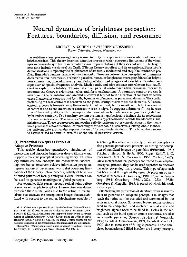
Figure 8 simulates a luminance profile with five cusps,using the same equations and parameters that generateFigure 7. The activity pattern in Figure 8d is much flatter than one might expect from the step-like pattern inFigure 7d. Coren (1983) found a similar result with thistype of stimulus. Figure 7 suggests that the result of Coren(1983), which he attributes to cognitive factors, may bepartially explained by feature-contour and boundarycontour interactions due to a single spatial scale.
Such a single-scale reaction does not, however, exhausteven the noncognitive monocular interactions that arehypothesized to occur within our theory. The existenceof multiple spatial scales has been justified from severalpoints of view (Graham, 1981; Graham & Nachmias,1971; Grossberg, 1983b; Kaufman, 1974; Kulikowski,1978). The influence of these multiple scale reactions arealso suggested by some displays of Arend et al. (1971).One such display is redrawn in Figure 9. The transformation of cusp in Figure 9a into step in Figure 9b andthe computation of the relative contrast of the incrementson their backgrounds are easy for the single-scale networkthat simulates Figures 7 and 8. This network cannot,however, generate the same brightness on both sides ofthe increments in Figure 9b, because the boundarycontour signals due to the increments prevent the featurecontour signals due to the cusps from diffusing across theincrements. Thus, to a single-scale network, the left andright distal brightnesses appear more equal than the brightnesses on both sides of the cusps.
(a)
Figure 9. The luminance profile in (a) generates the brightnessprofile in (b). (Redrawn with permission from Arend, Buehler, &Lockhead, 1971.)
This difficulty is partially overcome when multiple spatial scales (viz, separate shunting on-center off-surroundnetworks with different intercellular interaction coefficients) process the same input pattern, and the perceivedbrightness is derived from the average of all the resultantactivity patterns across their respective syncytia. In thissetting, a low-frequency spatial scale may generate aboundary contour in response to the cusp, but not inresponse to the increments (Grossberg, 1983b). Themonocular brightness pattern generated by such a scaleis thus a single step centered at the position of the cusp.When this step is averaged with the monocular brightness pattern of a high-spatial-frequency scale, the difference between proximal and distal background brightnessestimates becomes small relative to the difference betweenstep and background brightnesses. This explanation ofFigure 9 may be testable by selectively adapting out thehigh- or low-spatial-frequency scales.
The action oflow-spatial-frequency scales can also contribute to the flattening of the perceived brightnesses induced by a five-cusp display. Five cusps activate a broadernetwork domain than do two cusps of equal size. Lowspatial-frequency scales that do not significantly react totwo cusps may generate a blob-like reaction to five cusps.When such a reaction is averaged in with the already flattened high-spatial-frequency reaction, an even flatter percept can result.
(10) Smoothly Varying Luminance Contours vs.Steps of Luminance Change
Bergstrom (1966, 1967a, 1967b) has collected data thatrestrict the generality of the conclusion that sharp edgescontrol the perception of brightness. In those experiments,he compared the relative brightness of several luminancedisplays. Some of the displays possessed no sharp luminance edges within their interiors. Other displays didpossess sharp luminance edges. Bergstrom used a variant of the rotating prism method to construct twodimensional luminance distributions in which the luminance changed in the horizontal direction but was constant in each narrow vertical strip. The horizontal changesin two such luminance distributions are shown inFigure 10.
Figure lOa depicts a luminance profile wherein the luminance continuously decreases from left to right. Bergstrom constructed this profile to quantitatively test the theory of Mach (1866) that attributes brightness changes tothe second derivative d2L(x)/dx2with respect to the spatial variable x of the luminance profile L(x) (see Ratliff,1965). Mach (1866) concluded that, if two adjacent pointsx, and X3 have similar luminances [Ltx.) =:: L(x3)], thenthe point X3 at which the second derivative is negative{[d2(x3)/dx2] < O}, looks brighter than the point x, atwhich the second derivative is positive {[d2L(x
l)ldx2] >
O}, and that a transition between a darker and a lighterpercept occurs at the intervening inflection point X2{[ct2L(x2)/dx2] = O}. In Figure lla, as Mach wouldpredict, the position X3 to the right of X2 looks brighterthan the position x, to the left of X2. Figure 11a describes

NEURAL DYNAMICS OF BRIGHTNESS PERCEPTION 439
x; x; x;
Figure 10. Two luminance profiles studied by Bergstrom. Position X3 of (a) looks brighter than position xf of (b). Also positionX3 looks brighter than position x, in (a), and position xtIooks somewhat brighter than position xf in (b). These data challenge thehypothesis that sharp edges determine the level of brightness. Theyalso challenge the hypothesis that a sum of spatial-frequency-fIlteredpatterns determines the level of brightness.
80 • .A
en 70 • .BenwZ60I-::J:S2 50a:m
40w>~ 30
o~ 20m;:)en , , , ,
1 2 34 5 67 8 9 10 11 12
SPACE
shows that position xtlooks darker, not brighter, than position X3. These data cast doubt on the conclusionof Arendet al. (1971), just as the data of Arend et al. cast doubton the conclusion of Mach (1866).
Our numerical simulations reproduce the main effectssummarized in Figures 10 and 11. The critical feature ofthese simulations is that the two luminance profiles inFigure 10 generate different boundary-contour patternsas well as different feature-contour patterns. The luminance profile of Figure 12a generates boundary contours only at the exterior edges of the luminance profile(Figure 12b). By contrast, each interior step of luminanceof Figure l3a also generates a boundary contour (Figure l3b). Thus, the monocular perceptual domains thatare defined by the two luminance profiles are entirelydifferent. In this sense, the two profiles induce, and areprocessed by, different perceptual spaces. These different parsings of the cell syncytium not only define different numbers of spatial domains, but also different sizesof domains over which featural quality can spread.
In addition, the smooth vs. sharp contours in the twoluminance profiles generate different feature-contour patterns (Figures 12c and l3c). The differences between thefeature-contour patterns do not, however, explain Bergstrom's data, because the feature-contour pattern at position xt in Figure l3c is more intense than the featurecontour pattern at position X3 in Figure 12c. This is theresult one would expect from classical analyses of contrast enhancement. By contrast, when these featurecontour patterns are diffusively averaged between theirrespective boundary contours, the result of Bergstrom isobtained. The monocular brightness pattern at positionX3 in Figure 12d is more intense than the monocularbrightness pattern at position xtin Figure l3d. We therefore concur with Bergstrom in his claim that these resultsare paradoxical from the viewpoint of classical notionsof brightness contrast. We know of no other brightness
Figure 11. Magnitude estimates of brightness in response to theluminance profiles of Figure 10. (Redrawn from Bergstrom, 1966.)
(a)
the results of a magnitude-estimation procedure that wasused to determine the brightnesses of different positionsalong the luminance profile. For details of this procedure,Bergstrom's original articles should be consulted.
Figure 11a challenges the hypothesis that brightnessperception depends exclusively upon difference estimatesat sharp luminance edges. No edge exists at the inflection point X2, yet a significant brightness difference isgenerated around position X2' Moreover the brightnessdifference inverts the luminance gradient, since x, is moreluminous than X3, yet X3 looks brighter than x..
One might attempt to escape this problem by claimingthat, although the luminance profile in Figure lOa contains no manifestedges, the luminancechanges sufficientlyrapidly across space to be edge-like with respect to somespatial scale. This hypothesis collapses when the luminance profile of Figure lOb is considered. The luminance profile of Figure lOb is constructed from the luminance profile of Figure lOa as follows. The luminancein each rectangle of Figure lOb is the average luminancetaken across the corresponding positions of Figure lOa.Unlike Figure IOa, however, Figure lOb possessesseveral sharp edges. If the hypothesis of Arend et al.(1971) is taken at face value, then position xt ofFigure lOb should look brighter than position X3 ofFigure lOa. This is because mean luminances are preserved between the two figures and Figure lOb has sharpedges, whereas Figure lOa has no interior edges whatsoever.
A magnitude estimation procedure yielded the datashown in Figure l lb. Comparison of Figures 11a and l lb

440 COHEN AND GROSSBERG
theory that can provide a principled explanation of boththe Arend et al. (1971) data and the Bergstrom (1966,1967a, 1967b) data.
In particular, both types of data cause difficulties forthe Fourier theory of visual pattern perception as an ade-
quate framework with which to explain brightness percepts. For example, the low-frequencyspatialcomponentsin the two Bergstrom profiles in Figure 10 are similar,whereas the step-like contour in Figure lOb also containshigh-spatial-frequency components. One might therefore
BERGSTROM BRIGHTNESS PARADOX (1)
.,.....---,(--------, r--
9.6*10'
-9.6*10'
INPUT PATTERN
POS
a
FEATURE CONTOUR PATTERN
c
1.0*10'
700
-1.0*10'
5.1*10'
700
-5.1*10'
BOUNDARY CONTOUR PATTERN
POS
b
MONOCULAR BRIGHTNESS
PATTERN
POS
d
700
Figure 12. Simulation of a Bergstrom (1966) brightness experiment. 1be input pattern (a) generates boundary contours in (b) only around the luminance profile as a whole. Bycontrast, the input pattern in Figure 13agenerates boundary contours around each step in luminance (Figure 13b). The input patterns in Figures12a and 13a thns determine different syncytial domains within which featural filling-in can occur. Theinput patterns in Figures 12a and 13a also determine different feature-contour patterns (Figures 12c and13c). The feature-contour pattern in Figure 13c is more active at position xhhan is the feature-contourpattern of Figure 12c at the corresponding position x3 • (See Figure 10 for definitions of X3 and x:.) Thefeature-contour pattern of Figure 12cdiffuses within the syncytial domains of Figure 12b, and the featurecontour pattern of Figure 13c diffuses within the syncytial domains of Figure 13b. The resultant brightness pattern of Figure 12d is more active at position X3 than is the brightness pattern of Figure 13d atposition x:. This feature-to-brightness reversal is due to the fact that the boundary-contour patterns andfeature-contour patterns induced by the two input patterns are different. The global structuring of eachfeature-contour pattern within each syncytial domain determines the ultimate brightness pattern.

NEURAL DYNAMICS OF BRIGHTNESS PERCEPTION 441
BERGSTROM BRIGHTNESS PARADOX (2)
9.6.10·
INPUT PATTERN
POS
a
FEATURE CONTOUR PATTERN
700
-1.0.10'
5.1.10·
BOUNDARY CONTOUR PATTERN
r-- r---
1 POS 70
b
MONOCULAR BRIGHTNESS
PATTERN
o
POS
-9.6'10·
700
-5.1.10'd
Figure 13. Simulation of a Bergstrom (1966) brightness experiment. See caption of Figure 12.
expect positron X3 to look brighter than position xt',whereas the reverse is true. In a similar fashion, whena rectangular luminance profile is Fourier analyzed using the human modulation transfer function (MTF) , itcomes out looking like a Craik-O'Brien contour (Cornsweet, 1970). A Craik-O'Brien contour also comes outlooking like a Craik-O'Brien contour. Our explanation,by contrast, shows why both Craik-O'Brien contours andrectangular contours look rectangular.
Some advocatesof the Fourier approach have respondedto this embarrassment by saying that what the outputs ofthe MTF look like is irrelevant, since only the identityof these outputs is of interest. This argument has carefully selected its data. It does not deal with the problem
that the interior and exterior activities of a Craik-O'Briencontour are the same and differ from the activities of thecusp boundary, whereas the interior and boundary activities of a rectangle are the same and differ from the activities of the rectangle exterior. The problem is notmerely one of the equivalence between two patterns. Itis also one of the recognition of an individual pattern.These difficulties of the Fourier approach do not implythat multiple spatial scales are unimportant during visualpattern perception. Multiple scale processing does not,however, provide a complete explanation. Moreover, thefeature-contour processing within each scale needs to useshunting interactions, rather than the additive interactionsof the Fourier theory, in order to extract the relative con-

442 COHEN AND GROSSBERG
trasts of the feature-contour pattern (Appendix A and B;Grossberg, 1983b).
(11) The Assymmetry between BrightnessContrast and Darkness Contrast
In the absence of a theory to explain the Arend et al.and Bergstrom data, one might have hoped that a moreclassical explanation of these effects could be discoveredby a more sophisticated analysis of the role of contrastenhancement in brightness perception. In both paradigms,it might at first seem that contrast enhancement aroundedges or inflection points could explain both phenomenain a unified way, if only a proper definition of contrastenhancement could be found. The following data ofHamada (1980) indicate, in a particularly vivid way, thatmore than a proper definition of contrast enhancement isneeded to explain brightness data.
Figure 14 depicts three luminance proftles. Figure 14a,a uniform background luminance is depicted. (Althoughthe background luminance is uniform, it is not, strictlyspeaking, a ganzfeld, for it is viewed within a perceptualframe.) In Figure 14b, a brighter Craik-O'Brien luminance proftle is added to the backgound luminance. InFigurel4c, a darker Craik-O'Brien luminance proftle issubtracted from the background luminance. The purityofthis paradigm derives from the facts that its two CraikO'Brien displays are equally long and that the background
(a)
(e)
Figure 14. The luminance contours studied by Hamada (1980).All backgrounds in (a)-(c) have the same luminance.
luminance is constant in all the displays. Thus, brightening and darkening effects can be studied uncontaminatedby other variables.
The classical theory of brightness contrast predicts thatthe more luminous edges in Figure 14b will look brighterthan the background in Figure 14a and that, due to brightness contrast, the background around the more luminousedges in Figure 14b will look darker than the uniform pattern in Figure 14a. This is, in fact, what Hamada found.The classical theory of brightness contrast also predictsthat the less luminous edges in Figure 14c will look darkerthan the background in Figure 14a and that, due to brightness contrast, the background around the less luminousedges in Figure 14c will look brighter than the backgroundin Figure 14a. Hamada (1980) found, contrary to classical theory, that both the dark edges and the backgroundin Figure 14c look darker than the background in Figure 14a. These data are paradoxical because they showthat brighter edges and darker edges are, in some sense,asymmetrically processed, with brighter edges elicitingless paradoxical brightness effects than darker edges.
Hamada (1976, 1978) developed a multistage mathematical model to attempt to deal with his challenging data.This model is remarkable for its clear recognition that a"nonopponent" type of brightness processing is neededin addition to a contrastive, or edge-extracting, type ofbrightness processing. Hamada did not define boundarycontours or diffusive filling-in between these contours,but his important model should nonetheless be betterknown.
Figures 15 and 16 depict a simulation of the Hamadadata using our theory. As desired, classicalbrightness contrast occurs in Figure 15, whereas as nonclassical darkening of both figure and ground occurs in Figure 16. Thedual action of signals from the BCS stage to the MBCstages as boundary-contour signals and as inhibitoryfeature-contour signals contributes to this result in oursimulations.
All of the results described up to now consider how activity patterns are generated within the MBCL and MBCRstages. In order to be perceived, these patterns must activate the BP stage. In the experiments already discussed,the transfer of patterned activity to the BP stage does notintroduce any serious constraints on the brightness properties of the FIRE model. This is because all the experiments that we have thus far considered present the sameimage to both eyes. The experiments that we now discuss present different combinations of images to the twoeyes. Thus they directly probe the process wherebymonocular brightness domains interact to generate abinocular brightness percept.
(12) Simulations of FIREIn the remaining sections of the article, we describe
computer simulations using the simplest version of theFIRE process and the same model parameters that wereused in Cohen and Grossberg (1984). We show that thismodel qualitatively reproduces the main properties of

NEURAL DYNAMICS OF BRIGHTNESS PERCEPTION 443
HAMADA BRIGHTNESS PARADOX (1)
INPUT PATTERN
POS
aFEATURE CONTOUR PATTERN
POS
c
6.0.10'
1700
-6.0.10'
1700
BOUNDARY CONTOUR PATTERN
POS
b
MONOCULAR BRIGHTNESS
PATTERN
d
1700
Figure 15. Simulation of the Hamada (1980) brightness experiment. The dotted line in (d) describes thebrightness level of the background in Figure 13a. Classical contrast enhancement is obtained in (d).
Fechner's paradox (Levelt, 1965), binocular brightnesssummation and averaging (Blake, Sloane, & Fox, 1981;Curtis & Rule, 1980), and a parametric brightness studyof Cogan (1982) on the effects of rivalry, nonrivalrysuppression, fusion, and contour-free images. Thus,although the model was not constructed to simulate thesebrightness data and does not incorporate many knowntheoretical refinements, it performs in a manner thatclosely resembles difficult data. We believe that thesesimulations place the following quotation from a recentpublication into a new perspective: "The emerging picture is not simple ... Levelt's theory ... works forbinocular brightness perception, but not for sensitivity toa contrast probe . . . it seems unlikely that any singlemechanism can account for binocular interactions . . . The
theory of binocular vision is essentially incomplete" (Cogan, 1982, pp. 14-15).
Before reporting simulations of brightness experiments,we review a few basic properties of this FIRE model. Allthe simulations were done on one-dimensional arrays ofcells, for simplicity. All the simulations use pairs of inputpatterns that have zero disparity with respect to each other.The reaction of a single spatial scale to these input patternswill be reported. Effects of using nonzero disparities andmultiple spatial scales are described in Cohen and Grossberg (1984) and Grossberg (1983b). The input patternsshould be interpreted as monocular patterns across MBCLand MBCR, rather than the scenic images themselves.
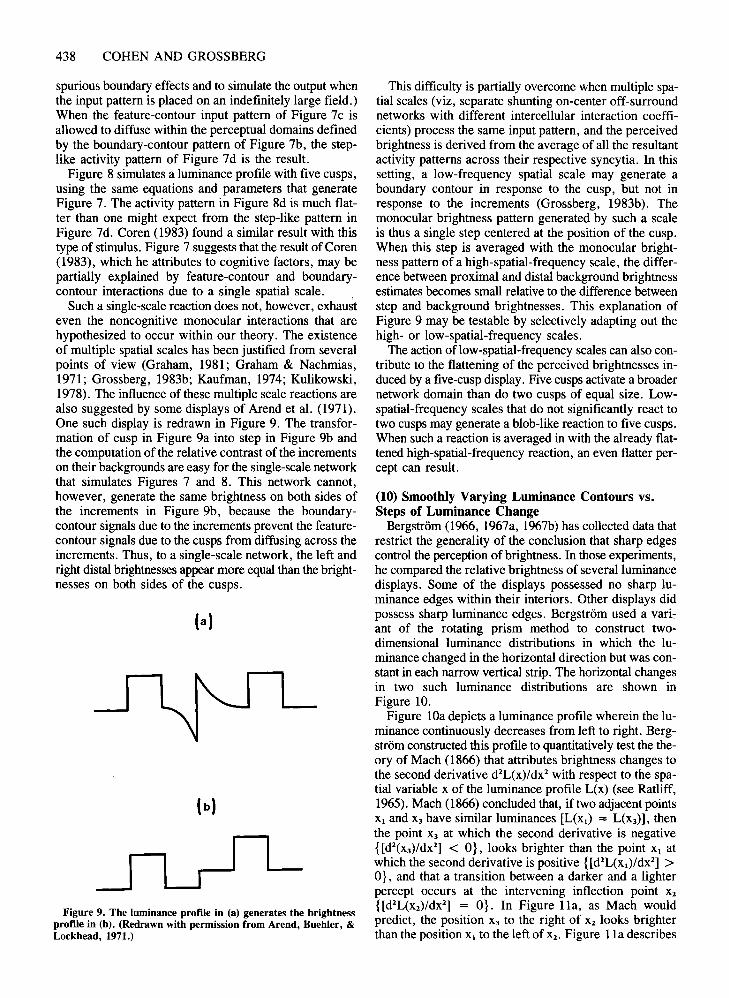
(a) Insensitivity to functional ganzfelds. In Figure 17,two identical input patterns exist at the MBCL and MBCR

444 COHEN AND GROSSBERG
HAMADA BRIGHTNESS PARADOX (2)
INPUT PATTERN
POS
a
FEATURE CONTOUR PATTERN
POS
c
6.0.10'
1700
-6.0.10'
1700
BOUNDARY CONTOUR PATTERN
POS
b
MONOCULAR BRIGHTNESS
PATTERN
d
1700
Figure 16. Simulation of the Hamada (1980) brightness experiment. The dotted line in (d) describes thebrightness level of the background in Figure 13a. Both background and cusp of (a) look darker than thisreference level.
stages (Figure 17a). Both input patterns are generated byputting a rectangular pattern through a Gaussian filter.This smoothing operation was sufficient to prevent thepathways MBCL - BP and MBCR- BP in Figure 4 fromdetecting suprathreshold contours in the input patterns.We call an input pattern that has no contours that are detectable by these pathways a "functional ganzfeld. " TheFIRE process does not lift functional ganzfelds at any input intensity. The simulationillustrates that the BP stage isinsensitive to input patterns that include no boundarycontours detectable by its filtering operations.
(b) Figure-ground synthesis: Ratio scale and powerlaw. Figure 18 describes the FIRE reaction that is triggered when a rectangular input pattern is superimposedupon a functional ganzfeld. Such an input pattern ideal-
izes a region of rapid change in activity with respect tothe network's filter bandwidth. The entire input patternis now resonantly lifted into the BP stage. Although theBP stage is totally insensitive to the functional ganzfeldtaken in isolation, the sharp edges of the rectangle trigger a resonant reaction that structures, indeed defines, thefunctional ganzfeld as a "ground" for the rectangular"figure." Instead of being treated as merely formlessenergy, the functional ganzfeld now energizes a standingwave that propagates from the rectangle edges to theperimeter of the pattern.
Due to the rectangle's edges, the network is now exquisitely sensitive to the ratio of rectangle-to-ganzfeld inputactivities. When the entire input pattern is parametricallyincreased by a common multiple, FIRE activity levels
NEURAL DYNAMICS OF BRIGHTNESS PERCEPTION 445
LEFT INPUT LEFT F·I ELD
POS
a
100
>....s....o-e POS
b
o
2.9*10'"MATCH FIELD • FILTERED MATCH FIELD
1.0.10
POS
c
100
>....s....o~ POS
d
Figure 17. Matched ganzfelds in (a) cause no suprathreshold reaction at the BP stage at any inputintensity. Left input in (a) denotes the input pattern that is delivered to both the MPLstage and theMPR stage. Left field in (b) denotes the activity pattern that is elicited at both the MBCL stage andthe MBCRstage. Match field in (c) denotes the activity pattern that is elicited at the BP stage. Filteredmatch field in (d) denotes the feedback signal pattern that is emitted from the BP stage to both theMBCL and MBCR stages. No feedback is elicited because the BP stage does not generate anysuprathreshold activities in response to the edgeless input pattern, or functional ganzfeld, in (a).(Reprinted from Cohen & Grossberg, 1984.)
obey a power law (Figure 19). Both the intensity of thestanding wave corresponding to the rectangle and theintensity of the standing wave corresponding to thefunctional ganzfeld grow as a power of their corresponding input intensities. In these simulations, the powerapproximates .8. This power is not built into the network.It is a collective property of the network as a whole.
(13) Fechner's ParadoxThe simplest version of Fechner's paradox notes that
the world does not look half as bright when one eye isclosed. In fact, suppose that a scene is viewed throughboth eyes but that one eye sees it through a neutral density filter (Hering, 1964). When the filtered eye is entirelyoccluded, the scene looks brighter and more vivid despitethe fact that less total light reaches the two eyes.
Another version of this paradox is described in
Figure 20 (Cogan, 1987; Levelt, 1965). Figures 20a-20cdepict three pairs of images. One image is viewed by eacheye. In Figure 20a, an uncontoured image is viewed bythe left eye and a black disk on a uniform backgroundis viewed by the right eye. In Figure 20b, black disks areviewed by both eyes. In Figure 20c, the interior of theleft disk is white. Given appropriate boundary conditions,the binocular percept generated by the images in Figure 20a looks about as dark as the binocular percept generated by the images in Figure 20b, despite the fact that abright region in Figure 20a replaces a black disk inFigure 20b. Figure 2Oc, by contrast, looks much brighter.
The input patterns that we used to simulate these imagesare displayed in Figures 20d-20g. These input patternsrepresent the images in only a crude way, because theinput patterns correspond to activity patterns across stagesMBCL and MBCR rather than to the images themselves.

LEFT FI ELD
446 COHEN AND GROSSBERG
LEFT· INPUT
130
5.3-10'"
\ l,q vV 130
-1.3.10-1 a b
6.5.10'"MATCH FIELD _. F I LTERED MATCH FIELD
3.6-10
>....S; R
~ 1 V~ '0
A
n
VV 130
>l-
s....t)-e
130
-6.5-10~
c dFigure 18. Figure on ganzfeld: The pair of sharp contours within the input pattern of (a) sensitizes the
BP stage to the activity levels of both the rectangle figure and the ground, despite the total insensitivityof the BP stage to a functional ganzfeld in Figure 17 at any input intensity. Binocular matching of thecontours at the BP stage lifts a standing wave representation (c) of figure and ground into the BP stage.(Reprinted from Cohen & Grossberg, 1984.)
It is uncertain how, for example, to choose the activityof the ganzfeld in Figure 20a, since this activity dependsupon the total configuration of contours throughout thefield of view. We therefore carried out a simulation usinga zero intensity ganzfeld, as well as a simulation with afunctional ganzfeld whose intensity equals the backgroundintensity of the input pattern to the the other MBC stage.The actual functional ganzfeld intensity should liesomewhere in between these two values. Other approximations of this type are used throughout the simulations.
The numbers listed in Figures 2Od-20g describe the totalrectified output from the FIRE cells that subtend the regioncorresponding to the black disk. As in the data, Figure 20ggenerates a much larger output than Figure 20f. Figure 20g also generates a larger output than either Figure 20d or Figure 20e. If the actual functional ganzfeldlevel is small due to the absence of nearby feature-contoursignals, then Figures 20a and 20b will look equally brightto the network.
A comparison between Figures 20d and 20e providesthe first evidence of a remarkable formal property of thisversion of the FIRE model. Although the FIRE processis totally insensitive to a pair of functional ganzfelds, whena functional ganzfeld is binocularly paired with acontoured figure, it can influence the overall intensity ofbinocular activity within the BP stage.
(14) Binocular Brightness Averagingand Summation
Experimental studies of the conditions under whichFechner's paradox hold have led to the conclusion that"binocular brightness should represent a compromisebetween the monocular brightnesses when the luminancespresented to the two eyes are grossly different and ...it should exceed either monocular brightness when theirluminances approach equality" (Curtis & Rule, 1980,p. 264). Curtis and Rule point out that "these results werein conflict with the prediction of averaging models, such

NEURAL DYNAMICS OF BRIGHTNESS PERCEPTION 447
,
h;
,,/' /v/ V
~
p. 31/~ V1/ /10/
,7f'
/v
~.YI\.'"
i/ r SI
7."AV ~ LEGEND
V o =BASEV 0= PEDESTAL
.> V INPUT
1/
f~~
1/ t;'/ -c
V pos
I i
III i
ii
iI
illIii
j1
I I IIII I !III I i I ! i I
1dSCALED INPUT
Figure 19. Power-law processing of figure and ground activity levels at the DP stage as theintensities of the input pattern (in the insert) are proportionally increased by a common factor.The abscissa (scaled input) measures this common factor. The ordinate (scaled activity) measures the peaks of DP activity at the rectangle (circles) and the ground (squares). (Reprintedfrom Cohen & Grossberg, 1984.)
as those of Engel (1969) and Levelt (1965)" (p. 263).They introduce a vector model to partially overcome thisdifficulty. Although the averaging and vector models areuseful in organizing brightness data, they do not providea mechanistic explanation of these data.
Figure 21 describes an example of binocular averaging by the FIRE process. In Figures 2la and 2lb, oneof the input patterns is a functional ganzfeld. The otherinput pattern is an increment or a decrement on a background. Since these monocular input figures differ greatlyin intensity, binocular brightness averaging should occurwhen they are binocularly presented. In Figure 2lc, theincrement input pattern is paired with a decrement inputpattern. The binocular figural activity in Figure 2lcalmost exactly equals the average of the monocular figuralactivities in Figures 2la and 21b.
In Figure 2ld, a pair of increment input patterns ispresented to the model. A comparison of Figure 2ld with
Figure 2la shows that the binocular figural activity inFigure 2ld is significantly greater than the monocularfigural activity in FiglJIi 2la; that is, binocular brightness summation has/occurred. Using these inputs, thebinocular brightness is about 25 % greater than themonocular brightness. Using a fully attenuated (zero)ganzfeld in one eye during the monocular condition, thebinocular brightness is about 63% brighter than themonocular brightness. Nonlinear binocular summation inwhich the binocular percept is less than twice as brightas the monocular percept has been described by a numberof investigators (Blake et al. 1981; Cogan et al., 1982;Legge & Rubin, 1981).
(15) Simulation of a Parametric BinocularBrightness Study
Cogan (1982) has analyzed binocular brightness interactions by studying a subject's sensitivity to monocular

448 COHEN AND GROSSBERG
FECHNER'S PARADOX5.0J410-3
nnnIDI
I-I D.D
nnIAI
lEI
O.D
'-'-I nnnnlSI IFI
101_17.1 "10-3
rmJ1JlICI IGI
Figure 20. Fechner's paradox: In human experiments based onthe images in (a)-(c), the left image is viewed by the left eye whilethe right image is viewed by the right eye. The simulations used thepairs of patterns in (d)-(g) as left and right input patterns to theFIRE process. Ganzfelds of different intensity are used as left input patterns to the FIRE model in (d) and (e). The FIRE activitylevels corresponding to the dark region positions in the right inputpatterns are printed above. In vivo, the ganzfeld intensity of a largefield will be close to zero at the MBCLstage, as in (e). In (0, identical left and right input patterns elicit zero FIRE activity in the darkregion. In (g), the dark region generates the largest FIRE activityof the series.
BRIGHTNESS AVERAGINGAND SUMMATION
IAI
test flashes while the subject binocularly views differentpairs of monocular images. Cogan used this method oflimits to obtain psychometric curves, and then rankordered paradigms in terms of subject sensitivity. Figure 22 describes the five conditions that Cogan studiedin his Experiment 2. In each condition, a brief disk-shapedflash was presented to the left eye. The flash area waschosen to fit exactly within the circular contour in the leftimage. Figure 23 describes the sensitivity of six different subjects to each of the five pairs of images. Meandetection sensitivity tended to rank-order the images fromFigure 22a to Figure 22e in order of decreasing sensitivity. Mean sensitivity to the images of Figure 22a wassignificantly greater than to the other images over a widerange of probe contrasts (.:lIlI). Mean sensitivity toFigure 22e was significantly less than to the other imagesover a wide range of probe contrasts. Mean sensitivityto the other images grouped more closely together. Therank orderings of individual observers did not, moreover,always decrease from Figure 22b to Figure 22d.
Simulations using the simplest one-dimensional inputversions of the images in Figure 22 tended to reproducethis pattern of results. Figure 24 illustrates the input pairsthat were used. Each input pair represents the flash condition. The increment above the background level on theleft input pattern represents the flash. To estimate flashvisibility, we first computed the figural activity within theflash area that was generated before the flash, then computed the figural activity within the flash area that wasgenerated during the flash, and then subtracted the beforeflash activity from the after-flash activity. The before-flash
FLASH DISPLAYS
~.
lSI
ICI
IDI
IAI
~o(CI
lSI
~.IDI
Figure 21. Brightness averaging and summation: The input pairin (c) generates a FIRE activity at their center that is approximatelythe average of the FIRE activities generated at the center positionsof the input pairs in (a) and (b). The input pair in (d) generates aFIRE activity that is greater at its center than the FIRE activitygenerated at the center of the input pattern in (a).
lEI
Figure 22. Flash displays used by Cogan (1982) to study binocular brightness processing. The dashed lines denote the regions thatreceive monocular flashes. Cogan tested the sensitivity of SUbjectsto flashes in the designated positions.

NEURAL DYNAMICS OF BRIGHTNESS PERCEPTION 449
FLASH PROFILES
crepancy with the data is due to the fact that sensitivityto the images in Figure 24d slightly exceeds that to theimages in Figures 24c and 24b. This type of order inversion also occurred, however, in two out of six of Cogan'ssubjects (Cogan, 1982, Figure 6, p. 11). Considering thesimplicity of the model and its input patterns, and the number of qualitatively correct effects that it can generate,this seems to be a relatively minor point.
Figure 25 displays the resonant patterns that are generated by four pairs of distinct monocular images. Figures25a and 25b illustrate the computer experiment in Figure 24d. In Figure 25a, a ganzfeld is paired with a blackdisk. Although the network is insensitive to a pair ofganzfelds (Figure 17), the black disk at the MBCRstagestructures and energizes the ganzfeld at the MBCL stagevia the BP stage. The structured ganzfeld, in turn,modifies the activity level at the BP stage. The monocular MBCR pattern remains inactive at cells that receivethe black input, despite the fact that the binocular FIREpattern is active within the corresponding region due tothe influence of the ganzfeld. Figure 25b adds an increment, or flash, to the ganzfeld in Figure 25a. Again, theMBCR pattern remains inactive at cells that receive theblack input. A comparison of Figures 25a and 25b shows,however, that the BP stage is sensitive to the activity levelsof both monocular patterns within this region. In fact, theactivity level in this region of the BP stage in Figure 25baverages the corresponding monocular activities.
Figures 26a and 26b illustrate the computer experimentin Figure 24e. Note that the dark contour in the MBCLinput pattern is detected by the resonance. This contourmonocularly energizes the binocular resonance in Figure 26a much more than does the ganzfeld of equal background intensity in Figure 25a.
ABC D EABC D E
>I-
;~Unkh.utLwen
Figure 23. Sensitivity of individual subjects to the flash displaysdescribed in Figure 22. Each bar height corresponds to a subject'ssensitivity to a particular flash display. The labels (A)-(E) refer tothe flash conditions in Figure 22. (Redrawn from Cogan, 1982.)
Figure 24. Flash profiles used to simulate the Cogan (1982) experiment. These profiles depict the profile when the flash is on. Before the flash is on, all the increments above the background luminance are absent.
activities, after-flash activities, and flash-induced activitydifferences are listed in Table 2. As in the data, the imagesin Figure 24a generated the largest increment, those inFigure 24e generated smallest increment, and the otherthree increments were clustered together. The main dis-
(16) Concluding RemarksThe results in this article suggest that several of the most
basic concepts of visual theory need to be refined. Forexample, the simulations described above include at leastthree mechanistically different concepts of contour:boundary contour, feature contour, and FIRE contour.They also include two different types of filling-in: diffusive filling-in, which is.rrionocular, and resonant fillingin, which is binocular: Although these concepts add somecomplexity to the visual modeling literature, they havebegun to simplify and unify the explanation of a large bodyof visual data. The same concepts have been used, forexample, to suggest explanations of data concerningmonocular and binocular rivalry, illusory figures, fading
Table 2Simulation of Brightness Experiment in Figure 24
Activity of Activity ofInner Region Inner Region Activity
Figure Before Flash During Flash Increment
24a .o00ooo .015740 .01574024b .012356 .016165 .00380924c .011824 .015689 .00386524d .005031 .008904 .00387324e .007075 .010407 .003332

450 COHEN AND GROSSBERG
(a) GANZFELD PLUS DARK FIGURE INCREMENT PLUS DARK FIGURE
LEFT FlELD RIGHT FlELD LEFT FlELD RIGHT FlELD
MATCH FlELD FlLTERED MATCH FIELD MATCH FlELD FlLTERED MATCH FlELD
Figure 25. FIRE patterns generated by the flash displays of Figure 24d; (a) Before flash FIRE pattern; (b) during flash FIRE pattern.Left field denotes the MBCL-stageactivity pattern. Right field denotes the MBCR-stageactivity pattern. Match field denotes the BP-stageactivity pattern. Filtered match field denotes the feedback signal pattern emitted by the BP stage to the MBCL and MBCR stages.
(a) BOUNDARY PLUS DARK FIGURE(b]
INCREMENT IN BOUNDARY
LEFT FlELD RIGHT FlELD LEFT FlELD RIGHT FlELD
MATCH FlELD FlLTERED MATCH FlELD MATCH FlELD FlLTERED MATCH FlELD
Figure 26. FIRE patterns generated by the flash display of Figure 24e. (a) Before flash FIRE pattern; (b) during flash FIRE pattern.

NEURAL DYNAMICS OF BRIGHTNESS PERCEPTION 451
of stabilized images, neon color spreading, illusory complementary color induction, the Land retinex demonstrations, nonlinear multiple scale interactions, and variousglobal interactions between depth, lightness, length, andform properties (Cohen & Grossberg, 1984; Grossberg,1980, 1983b, 1985; Grossberg & Mingolla, in press).Moreover, the concepts seem to have more than a formalexistence. Boundary contour and feature contour interactions can, for example, be interpreted in terms of recent physiological data concerning the orientationsensitive but color-insensitive hypercolurnn system in thestriate cortex and the orientation-insensitive but colorsensitive blob system in the striate cortex (Table 1; Grossberg & Mingolla, in press). It remains to be seen just howfar these new concepts and mechanisms can be developedfor the further explanation and prediction of complexvisual phenomena.
REFERENCES
AREND, L. E., BUEHLER, J. N., & LOCKHEAD, G. R. (1971). Difference information in brightness perception. Perception & Psychophysics, 9, 367-370
BERGSTROM, S. S. (1966). A paradox in the perception of luminancegradients, I. Scandinavian Journal of Psychology, 7, 209-224.
BERGSTROM, S. S. (l967a). A paradox in the perception of luminancegradients, II. Scandinavian Journal of Psychology, 8, 25-32.
BERGSTROM, S. S. (l967b). A paradox in the perception of luminancegradients, III. Scandinavian Journal of Psychology, 8, 33-37.
BLAKE, R., & Fox, R. (1974). Binocular rivalry suppression: Insensitive to spatial frequency and orientation change. Vision Research, 14,687-692.
BLAKE, R., SLOANE, M., & Fox, R. (1981). Further developments inbinocular summation. Perception & Psychophysics, 30, 266-276.
CARPENTER, G. A., & GROSSBERG, S. (1981). Adaptation and transmittergating in vertebrate photoreceptors. Journal of Theoretical Neurobiology, I, 1-42.
COGAN, A. L. (1982). Monocular sensitivity during binocular viewing. Vision Research, 22, 1-16.
COGAN, A. L., SILVERMAN, G., & SEKULER, R. (1982). Binocular summation in detection of contrast flashes. Perception & Psychophysics,31, 330-338.
COHEN, M. A., & GROSSBERG, S. (1984). Some global properties ofbinocular resonances: Disparity matching, filling-in, and figure-groundsynthesis. In P. Dodwell & T. Caelli (Eds.), Figural synthesis. Hillsdale, NJ: Erlbaum.
COREN, S. (1983). When "filling-in" fails. The Behavioral and BrainSciences, 6, 661-662.
CORNSWEET, T. N. (1970). Visual perception. New York: AcademicPress.
CURTIS, D. W., & RULE, S. J. (1980). Fechner's paradox reflects anonmonotone relation between binocular brightness and luminance.Perception & Psychophysics, 27, 263-266.
DAY,R. H. (1983). Neon color spreading, partially delineated borders,and the formation of illusory contours. Perception & Psychophysics,34, 488-490.
ENGEL, G. R. (1969). The auto-correlation function and binocular brightness mixing. Vision Research, 9, 1111-1130.
GELLATLY, A. R. H. (1980). Perception of an illusory triangle withmasked inducing figure. Perception, 9, 599-602.
GERRiTS, H. J. M., DE HAAN, B., & VENDRiCK, A. J. H. (1966). Experiments with retinal stabilized images: Relations between the observations and neural data. Vision Research, 6, 427-440.
GERRiTS, H. J. M. & TIMMERMAN, J. G. M. E. N. (1969). The fillingin process in patients with retinal scotomata. Vision Research, 9,439-442.
GERRITS, H. J. M., & VENDRICK, A. J. H. (1970). Simultaneous contrast, filling-in process and information processing in man's visualsystem. Experimental Brain Research, 11,411-430.
GRAHAM, N. (1981). The visual system does a crude Fourier analysisof patterns. In S. Grossberg (Ed.), Mathematicalpsychologyandpsychophysiology. Providence, RI: American Mathematical Society.
GRAHAM, N., & NACHMIAS, J. (1971). Detection of grating patterns containing two spatial frequencies: A test of single-channel and multiplechannel models. Vision Research, 11,251-259.
GREGORY, R. L. (1966). Eye and brain. New York: McGraw-Hill.GROSSBERG, S. (1975). A neural model of attention, reinforcement, and
discrimination learning. International Review of Neurobiology, 18,263-327.
GROSSBERG, S. (1980). How does a brain build a cognitive code? Psychological Review, 87, 1-51.
GROSSBERG, S. (1982a). Studies of mind and brain: Neural principlesof learning, perception, development, cognition, and motor control.Boston: Reidel Press.
GROSSBERG, S. (l982b). The processing of expected and unexpectedevents during conditioning and attention: A psychophysiological theory. Psychological Review, 89, 529-572.
GROSSBERG, S. (l983a). Neural substrates of binocular form perceptiom: Filtering, matching, diffusion, and resonance. In E. Basar,H. Flohr, H. Haken, & A. J. Mandell (Eds.), Synergetics ofthe brain.New York: Springer.
GROSSBERG, S. (l983b). The quantized geometry of visual space: Thccoherent computation of depth, form, and lightness. Behavioral andBrain Sciences, 6, 625-692.
GROSSBERG, S. (1984). Outline of a theory of brightness, color, andform perception. In E. Degreef & J. van Buggenhaut (Eds.). Trendsin mathematical psychology. Amsterdam: North-Holland.
GROSSBERG, S. (1985). Neural dynamics of depth, brightness, color,and form perception: A predictive synthesis. Manuscript submittedfor publication.
GROSSBERG, S., & MINGOLLA, E. (1985). Nonlinear competition, cooperation, and diffusion in the neural dynamics of visual perception. InB. D. Sleeman & R. J. Jarvis (Eds.), Proceedings ofthe Dundee conference on ordinary and partial differential equations, 1984. NewYork: Springer.
GROSSBERG, S., & MINGOLLA, E. (in press). Neural dynamics of formperception: Boundary completion, illusory figures, and neon colorspreading. Psychological Review.
HAMADA, J. (1976). A mathematical model for brightness and contourperception. Hokkaido Report of Psychology, HRP-11-76-17.
HAMADA, J. (1978). Antagonistic and non-antagonistic processes forthe lightness perception. Hokkaido Behavioral Science Report,HBSR-P-4.
HAMADA, J. (1980, July 6-12). Antagonistic and non-antagonisticprocesses in the lightness perception. Proceedings of XXII International Congress of Psychology, Leipzig.
HEGGELUND, P. & KREKUNG, S. (1976). Edge dependent lightness distributions at different adaptation levels. Vision Research, 16, 493-496.
HELMHOLTZ, H. VON (1962). Physiological optics. (1. P. C. Southall,Ed. & Trans.). New York: Dover.
HENDRiCKSON, A. E., HUNT, S. P., & Wu, J.-Y. (1981). Immunocytochemicallocalization of glutamic acid decarboxylase in monkey striate cortex. Nature, 292, 605-607.
HERiNG, E. (1964). Outlines ofa theory ofthe light sense. Cambridge,MA: Harvard University Press.
HORTON, J. C., & HUBEL, D. H. (1981). Regular patchy distributionof cytochrome oxidase staining in primary visual cortex of macaquemonkey. Nature, 292, 762-764.
HUBEL, D. H., & LIVINGSTONE, M. S. (1981). Regions of poor orientation tuning coincide with patches of cytochrome oxidase stainingin monkey striate cortex. Neuroscience Abstracts, 11th Annual Meeting, Los Angeles, 118.12.
HUBEL, D. H., & WIESEL, T. N. (1977). Functional architecture of rnacaque monkey visual cortex. Proceedings ofthe Royal Society ofLondon (B), 198, 1-59.
KANIZSA, G. (1974). Contours without gradients or cognitive contours?Italian Journal of Psychology, 1,93-113.

452 COHEN AND GROSSBERG
APPENDIX A
to the diffusive filling-in process. The inhibitory term S, is defined by the boundary-contour process in Equation 6 below.
ZEKI, S. (l983b). Colour coding in the cerebral cortex: The responsesof wavelength-selective and colour coded cells in monkey visual cortex to changes in wavelength composition. Neuroscience, 9 , 767-791.
(3)
(1)
(2)
nn
n
E (BCki- DEki)Ikk=\
n
A+ E (Cki+Eki)Ikk=l
Xi
- AXi +(B -Xi) E IkCki- (Xi +D) E IkEki.k=\ k=\
ddt Xi
Feature ContoursThe input pattern (I" 12 , ••• , In) is transformed into feature
contours via a feed-forward on-center off-surround network ofcells undergoing shunting, or membrane equation, interactions.The activity, or potential Xi, of the i' h cell in a feature-contourpattern is
The activity pattern (x, X2, ... , xn) is sensitive to both theamount and the direction of contrast in edges of the input pattern (Grossberg, 1983b). These feature-contour activities generate inputs of the form
Both the on-center ceofficients Cki and the off-surround coefficients Ekiare Gaussian functions of intercellulardistance 1k - i I.System 1 is assumed to react more quickly than the diffusivefilling-in process. Hence, we assume that each Xi is in approximate equilibrium with respect to the input pattern. Atequilibrium, (d/dtjx, =0 and
This appendix describes the neural network that was used tosimulate feature-contour and boundary-contour interactions. Thefollowing simulations were done on one-dimensional fields ofcells. The input pattern (I" 12 , ••• , In) is transformed into theoutput pattern (z, Z2, ... , zn) via the following equations.
Boundary ContoursThe input pattern (I" 12 , ••• , In) also activates the boundary
contour process, which we represent as a feed-forward on-centeroff-surround network undergoing shunting interactions. Thissimplified view of the boundary-contour process is permissiblein the present simulations because the simulations, being onedimensional and monocular, do not need to account for orientational tuning, competition, or binocular matching. Since thesimulations do not probe the dynamics of illusory contour formation, the boundary completion process can also be ignored.(See Grossberg & Mingolla, in press, for these extensions.)
As in Equation 2, the intput pattern rapidly gives rise to anactivity pattern
KAUFMAN, L. (1974). Sight and mind: An introduction to visual perception. New York: Oxford University Press.
KENNEDY, 1. M. (1978). Illusory contours and the ends of lines. Perception, 7, 605-607.
KENNEDY, J. M. (1979). Subjective contours, contrast, and assimilation. In C. F. Nodine & D. F. Fisher (Eds.), Perception and pictorial representation. New York: Praeger Press.
KENNEDY, J. M. (1981). Illusory brightness and the ends of petals:Change in brightness without aid of stratification or assimilation effects. Perception, 10, 583-585.
KULIKOWSKI, J. J. (1978). Limit of single vision in stereopsis dependson contour sharpness. Nature, 275, 126-127.
LAND, E. H. (1977). The retinex theory of color vision. ScientificAmerican, 237, 108-128.
LEGGE, G. E., & RUBIN, G. S. (1981). Binocular interactions insuprathreshold contrast perception. Perception & Psychophysics, 30,49-61.
LEVELT, W. J. M. (1965). On binocular rivalry. Soesterberg: Institutefor Perception, RVO-TNO.
LIVINGSTONE, M. S., & HUBEL, D. H. (1982). Thalamic inputs tocytochrome oxidase-rich regions in monkey visual cortex. Proceedings of the National Academy of Sciences, 79, 6098-6101.
MACH, E. (1866). Uber die Wirkung der raumlichen Verteilung desLichtreizes auf die Netzhaut. Sitzungsber. Akad. Wiss., Mathemnaturwiss. st., Abt. 2, 52, 303-322.
O'BRIEN, V. (1958). Contour perception, illusion, and reality. Journalof the Optical Society of America, 48, 112-119.
PARKS, T. E. (1980). Subjective figures; Some unusual concomitantbrightness effects. Perception, 9, 239-241.
PARKS, T. E., & MARKS, W. (1983). Sharp-edged vs. diffuse illusorycircles: The effects of varying luminance. Perception & Psychophysics,33, 172-176.
PETRY, S., HARBECK, A., CONWAY, 1., & LEVEY, J. (1983). Stimulusdeterminants of brightness and distinctions of subjective contours. Perception & Psychophysics, 34, 169-174.
PRITCHARD, R. M. (1961). Stabilized images on the retina. ScientificAmerican, 204, 72-78.
PRITCHARD, R. M., HERON, W., & HEBB, D. O. (1960). Visual perception approached by the method of stabilized images. CanadianJournal of Psychology, 14, 67-77.
RATLIFF, F. (1965). Mach bands: Quantitative studies on neural networks in the retina. New York: Holden-Day.
REDIES, C. & SPILLMANN, L. (1981). The neon color effect in the Ehrenstein illusion. Perception, 10, 667-681.
RIGGS, L. A., RATLIFF, F., CORNSWEET, J. C., & CORNSWEET, T. N.(1953). The disappearance of steadily fixated visual test objects. Journal of the Optical Society of America, 43, 495-501.
SCHNEIDER, W., & SHIFFRIN, R. M. (1977). Controlled and automaticinformation processing, I: Detection, search, and attention. Psychological Review, 84, 1-66.
TODOROVIC, D. (1983). Brightness perception and the Craik-O-BrienComsweet effect. Unpublished M.A. Thesis. Storrs: University ofConnecticut.
VAN DEN BRINK, G., & KEEMINK, C. J. (1976). Luminance gradientsand edge effects. Vision Research. 16, 155-159.
VAN TUIJL, H. F. J. M. (1975). A new visual illusion: Neonlike colorspreading and complementary color induction between subjective contours. Acta Psychologica, 39, 441-445.
VAN TUIJL, H. F. J. M., & DE WEERT, C. M. M. (1979). Sensory conditions for the occurrence of the neon spreading illusion. Perception,8, 211-215.
VON DER HEYDT, R., PETERHANS, E., & BAUMGARTNER, G. (1984).Illusory contours and cortical neuron responses. Science, 224,1260-1262.
YARBUS, A. L. (1967). Eye movements and vision. New York: PlenumPress.
ZEKI, S. (l983a). Colour coding in the cerebral cortex: The reactionof cells in monkey visual cortex to wavelengths and colours. Neuroscience, 9, 741-765.

NEURAL DYNAMICS OF BRIGHTNESS PERCEPTION 453
Yi
E (BCki - DEki)Ikk=l
n
A + E (Cki+Eki)Ikk=1
(4)
tivity between compartments are less accessible to the signalsS, than are the exterior surface membranes that bound the cellular syncytium.
The following parameters were used in all the simulations withEquations 1-9. We let
(1) Two-Step and Five-Step Illusions (Figures 7 and 8)
where A = I, B = 96, C = .0625, E = .0625, G = .2349,H = 1, A = I, B = 35.5546, C = 50, D = 12.5828, E =50, /3 = 4x 10'°, 'Y = 5, 0 = 1 X 10'°, P. = .5, v = 1.5.
The remaining parameters vary from simulation to simulation and will be given for each figure by title.
where Cki and Eki are Gaussian functions of intercellular distance. It is assumed that these boundary contours are narrowerthan the feature contours defined by Equation 2.
The activity pattern (y" y2, ... , yn) is sensitive both to thedirection and amount of contrast in the input pattern (I" 12, ... ,In). The sensitivity to the direction of contrast is progressivelyeliminated by the following operations. Let the output signalsfrom BCS to MBC that are elicited by activity yi equal ftyr), andwhere f(w) is a sigmoid signal of the rectified part of Yi; viz,
(5)
The notation [w]' = max(w,O) and-y > 1. The output signalsf(Yi) are spatially distributed before influencing cell compartments of the cell syncytium. The total signal to the ith cell compartment due to the activity pattern (y" y2, . . . , yn) is
C;k = C expl e-In 2[(i-k)/JL]2j,
Eik = E expl s-In 2[(i-k)/v]'j,
Cik = C exp{-In 2[(i - k)/~]2j,
Eik = E expl v-In 2[(i-k)/V]2j,
Gik = G expl e- ln 2[(i - k)/W]2j,
n
EGikf(Yk),k=1
(6)n = 3,500,
D = 9.12,
where Gik is a Gaussian function of intercellular distance. ThisGaussian falloff is less narrow than that of boundary contoursin Equation 4, but more narrow than that of feature contoursin Equation 2.
Diffusive Filling-InThe activity z, of the ith cellular compartment of the cellular
syncytium obeys the nonlinear diffusion equation
where the input Fi is defined by Equation 3. The diffusion coefficients Ji + l,i and Ji - l,i are determined by boundary contour signals according to equations of the form
ct = 1,
Po = 10,
/I = 100,
A = 1.926 X 10⁶,
J( = 1.926 X 10⁷,
w = 1,
I' = 1.7.
The inputs. The inputs consist of a step input filtered througha Gaussian kernel with a set of ramping functions superimposedon the output of the filter. The steady state level of the outputis extended outward to simulate viewing the central portion ofan indefinitely large field with ramps superimposed. In the twocusp pattern of Figure 7a,
and
Ji + I,i = [S T'I]++ [S T'I]+I+J( i+1-1 J( i-I(8) Ik = 4>(k-350flOO) - 4>(k-3150/100) + R~2>,
where
where the threshold I' > O. Thus, an increase in the boundarysignal Si decreases both diffusion coefficients Ji + l,i and Ji - Ll
The feature-contour signal Fi also decreases when the boundary signal Si increases. In Equations 3, 8, and 9, the inhibitoryeffects of boundary signals S: on cell compartment membranesact via shunting inhibition. A positive threshold I' occurs inEquations 8 and 9, but not in Equation 3, because, we assume,the intercompartmental membranes that regulate diffusion of ac-
Ji- I,i = [S T'I]1+J([Si-1-I'j'+J( i-I +(9)
4>(x)
and
R ( 2 ) k -
{
o.12 tan[.9>r/2(l451-kIl49)]/tan[.91T/J
.12 tan[.91T12( 1750.5 - k/149.5)]!tan[.91T/2]
.12 tan[.9,../2(2050-k/149)]/tan[.9,../2]
o
if 0 ~ k ~ 1450
if 1451 ~ k ~ 1600
if 1601 ~ k ~ 1900
if 1901 s k s 2050
if 2051 ~ k ~ 3500.

454 COHEN AND GROSSBERG
In the five-cusp pattern of Figure 8a, II = 6,
Ik = <I>(k-350/100)I<1>(k-3150/100) + RkS)
where
}... = 6000,
x = 500,
w = 1,
r = 1.6.
(3) Bergstrom Brightness Paradox (Figures 12 and 13)
n = 700
D = 12,
Ik = .3<1>(k-351/100)-.3<1>(k-1350/100)+Pk,
The inputs. The inputs were chosen to simulate Hamada'sexperimental displays. The inputs consist of a step input filteredthrough a Gaussian filter with a parabolic segment superimposedon the output of this filter. Specifically, in Figure 15a, let
if 0 :s k :s 750
if 751 :s k :s 950
if 951 :s k :s 1700.
where
p,. I:05454{850.'-k199.'"
In Figure 16a,
if 0 :s k :s 1000
if 1001 :s k :s 1450
if 1451 :s k :s 1750
if 1751 :s k :s 2050
if 2051 :s k :s 2350
if 2351 :s k :s 2650
if 2651 :s k :s 2800.
if 2801 :s k :s 3500.
o.12 tan[.911"/2(lool-k/149)]/tan[.911"/2]
.12 tan[.911"/2(1600.5 - k/149.5)]/tan[. 911"12]
.12 tan[.911"/2(19oo.5 - k/149.5)]/tan[.911"12]
.12 tan[.911"/2(23oo.5 - kI149.5)]/tan[.911"/2]
.12 tan[.911"/2(25oo.5 - k1149.5)]/tan[. 911"/2]
. 12 tan[.911"/2(2800- k/149)]/tan[.911"/2]
o
a = 4, Ik = .3<1>(k-351/100)-.3<1>(k-1350/l00)-Pk.
/L = 10,
II = 60,
}... = 1000,
x = 116.7,
w = 10,
r = 2.6.
APPENDIX B
The following system of equations defines a binocular interaction capable of supporting a filling-in resonant exchange, orFIRE (Cohen & Grossberg, 1984; Grossberg, 1983b).
The inputs. The inputs represent Bergstrom's experimentalinputs. The inputs consist of two normal curves splined togetherat ±3 standard deviations away from the 50 percentile pointand placed on a pedestal. Thus, in Figure 12a,
Left Field:
Monocular Representations
I~6 + .4<1>(3(l-(k-149/100)))
.2+ .4<1>(3(1-(k-349/100»)
o
if 0 :s k -s 149
if 150 :s k :s 349
if 350 :s k :s 549
if 550 :s k :s 700.
d n
dt XiL = -AXiL +(B-xid E IkdJkL +Zk]+Ckik=l
n
- (XiL + D) E IkL[JkL +zk]+Ekik=l
(10)
In Figure 13a, the inputs were chosen to be four steps of length100 whose value is equal to the corresponding average valuein the previous set of runs. Thus,
0 if 0 :s k :s 150
.94 if 150 :s k :s 249
.60 if 250 :s k :s 349I k =
.54 if 350 :s k :s 449
.26 if 450 :s k :s 549
0 if 550 :s k -s 700.
and right field:
n
-(XiR + D) EIkR[hR +Zkj'Eki (11)k=!
where [w]+ = max(w,O).
(3) Hamada Brightness Paradox (Figures 15 and 16)Binocular Matching (Match Field)
n = 700,
D = 14.4,
a = 1,
/L = 1,
Yi =
n
E Fki[f(xkL) +f(XkR)]k=!
n
A+ EGki[f(xkL)+f(xkR)]k=l
(12)

NEURAL DYNAMICS OF BRIGHTNESS PERCEPTION 455
where
and
tive signals (15) with the same spatial bandwidths as are usedthroughout the computation. The parameters used in these simu-
(13) lations are exhaustively listed in Cohen and Grossberg (1984).The parameters used herein are the same as the parameters
used in simulations 15-23 of Cohen and Grossberg (1984), except that in the present simulations we chose n = 200.
(14)
Binocular-To-Monocular Feedback (Filtered Match Field)
InputsThe inputs are defined in terms of the functions
Equation 10 describes the response of the activities XiL, i = 1,2, ... , n, in the left monocular representation. Each XiL obeysa shunting equation in which both the excitatory interactioncoefficients Cki and the inhibitory interaction coefficients Ekiare Gaussian functions of the distance between Vk and Vi. Twotypes of simulations have been studied:
Additive inputs. All IkL are chosen equal. The terms JkLregister the input pattern and summate with the binocular-tomonocular feedback functions Zk. This is the form of the system that appears in the simulations reported herein.
Shunting inputs. All JkL are chosen equal. The terms IkLregister the input pattern. The binocular-to-monocular feedbackfunctions Zk modulate the system's sensitivity to the inputs IkLin the form of gain control signals.
Equation 11, for the activities XiR, i = 1,2, ... , n, in theright monocular representation, has a similar interpretation. Notethat the same binocular-to-monocular feedback functions Zk arefed back to the left and right monocular representations.
The binocular matching stage (12) obeys an algebraic equation rather than a differential equation due to the simplifyingassumption that the differential equation for the matching activities Yi reacts quickly to the monocular signals f(xkL) andf(xkR). Consequently, Yi is always in an approximate equilibriumwith respect to its input signals. This equilibrium equation saysthat the monocular inputs f(xkd and f(xkR) are added beforebeing matched by the shunting interaction. The signal functionsfew) are chosen to be sigmoid functions of activity w. The excitatory interaction coefficients Cki and inhibitory interactioncoefficients Ekiare chosen to be Gaussian functions of distance.The spatial decay rates of Cu. Cki, and C~i are chosen equal.The spatial decay rates of Eki, Eki, and E~i are chosen equal.The on-center is chosen narrower than the off-surround.
After the monocular signal patterns (f(XIL), f(x2d, ... , f(xnL))and (f(xlR), f(x2R), ... , f(xnR)) are matched at the binocularmatching stage, the binocular activities Yk are rectified by theoutput signal function g(Yk), which is typically chosen to be asigmoid function of Yk. Then these rectified output signals aredistributed back to the monocular representations via competi-
u r s r s soif 81 -s k :s: 120
if 121 -s k -s 200.
ifl:s:k:s:80
if 81 :s: k :s: 120
if 121 -s k :s: 200.
if 1 -s k :s: 70
if 71 :s:k:s: 80
if 81 :s:k:s: 120
if 121 :s: k :s: 130
if 131 :s:k :s:200
if 1 :s: k -s 70
if 71 -s k :s: 130
if 131 -s k :s: 200.
if 81 -s k -s 120
if 121 -s k -s 200.
Nk = .025c1>h/1/5(k -15)] - .025c1> [..j1/5(k -186)].
hR = FNk
(F) Let
hL = hR F'Nk
(G) Let
(E) Let JkL = 0, 1 -s k :s: 200, and
if 1 :s: k :s: 80
if 81 :s: k :s: 120
if 121 -s k :s: 200.
and
(A) Let hR = Ne. 1 :s: k :s: 200, and
[
Nk if 1 :s: k :s: 80
hL Nk+ .009 if 81 :s: k :s: 120
Nk if 121 :s: k :s: 200.
(B) Let hR = N, 1 :s: k :s: 200, and
if 1 .s k :s: 80
Fechner's Paradox (Figure 20):
(D) Let JkL = Nk, 1 -s k :s: 200, and
Brightness Averaging and Summation (Figure 21):
(15)
(16)
(17)
n
EF~ig(Yk)k=l
n
A*+ E G~ig(Yk)k=l
z,
where
and

456 COHEN AND GROSSBERG
(C) Let and
Boundary Plus Dark Figure (Figure 26a):
r iflsks80
hL = Nk+.OO9 if 81 s k s 120
Nk if 121 s k s 200
and
F' iflsks80
JkR = if 81 s k s 120
Nk if 120 s k s 200.
(D) Let
!Nk if 1 s k s 80
Nk+.OO9 ~f 81 -s k s 120
Nk If 121 s k -s 200.
The input patterns in Figures 24d and 24e are listed below toillustrate the parameter choicesused in this figure and to characterize the FIRE patterns depicted in Figure 25.
Let
and
u i s x s soif 81 -s k -s 120
if 121 s k s 200.
Nk if 1 s k s 70
0 if 71 s k s 80
Nk if 81 s k -s 120
0 if 121 -s k s 130
Nk if 131 s k -s 200
F'if 1 -s k s 70
if 71 s k -s 130
Nk if 131 s k s 200.
Ganzfeld Plus Dark Figure (Figure 25a):Increment in Boundary (Figure 26b):
Increment Plus Dark Figure (Figure 25b):
Nk if 1 s k -s 70
0 if 71 s k s 80
Nk+.OO9 if 81 s k s 120
0 if 121 s k -s 130
Nk if 131 -s k s 200
F'if 1 s k s 70
if 71 s k s 130
Nk if 131 -s k s 200.
JkL =
Let
and
iflsks80
if 81 -s k s 120
if 121 s k s 200
if 81 s k s 120
if 121 -s k s 200.
JkL =
Let
Let hL = Nk' 1 s k s 200, and
iflsks80
(Manuscript received March 23, 1984;revision accepted for publication August 20, 1984.)