NBER WORKING PAPER SERIES

THE END OF AMERICAN EXCEPTIONALISM?MOBILITY IN THE U.S. SINCE 1850

Joseph P. Ferrie

Working Paper 11324http://www.nber.org/papers/w11324

NATIONAL BUREAU OF ECONOMIC RESEARCH1050 Massachusetts Avenue

Cambridge, MA 02138May 2005

The views expressed herein are those of the author(s) and do not necessarily reflect the views of the NationalBureau of Economic Research.

©2005 by Joseph P. Ferrie. All rights reserved. Short sections of text, not to exceed two paragraphs, maybe quoted without explicit permission provided that full credit, including © notice, is given to the source.

The End of American Exceptionalism? Mobility in the U.S. Since 1850Joseph P. FerrieNBER Working Paper No. 11324May 2005JEL No. N0, J0

ABSTRACT

New longitudinal data on individuals linked across nineteenth century U.S. censuses document the

geographic and occupational mobility of more than 75,000 Americans from the 1850s to the 1920s.

Together with longitudinal data for more recent years, these data make possible for the first time

systematic comparisons of mobility over the last 150 years of American economic development, as

well as cross-national comparisons for the nineteenth century. The U.S. was a substantially more

mobile economy than Britain between 1850 and 1880. But both intergenerational occupational

mobility and geographic mobility have declined in the U.S. since the beginning of the twentieth

century, leaving much less apparent two aspects of the “American Exceptionalism” noted by

nineteenth century observers.

Joseph P. FerrieDepartment of EconomicsNorthwestern UniversityEvanston, IL 60208-2600and NBERferrie@northwestern.edu

1 Shafer (1999) traces the concept’s evolution.

Americans have from the very outset seen their nation as “exceptional.” In 1630, John

Winthrop, governor of the Massachusetts Bay Colony, famously proclaimed in a sermon at sea

that the settlers’ efforts would produce “a city on a hill,” an example to the world, even before

the Arabella landed at Salem with the colony’s second contingent of settlers (Winthrop, 1630

[1995], p. 111). Since then, the notion of “American Exceptionalism” has taken on a variety of

meanings.1 One of the most significant has been the belief that in the U.S., history is not destiny:

without a hereditary aristocracy or caste system or controls on internal migration, Americans are

less constrained than others by their family background in shaping their own lives. These beliefs

have, in the opinion of many scholars, helped shape American attitudes toward government and

prevent the development of a radical labor movement in the U.S.

This particular sense of U.S. exceptionalism was increasingly accepted as, throughout the

nineteenth century, many astute observers noticed the extremely high degree of social mobility in

the United States. As Alexis de Tocqueville toured the 1830s America of flatboats and family

farms, of busy workshops and loaded wharves, and of bustling cities and teeming canals, the

French aristocrat marveled at the economic activity. But he marveled even more at the

extraordinary fluidity of the social relations that lay beneath the economic tumult. Tocqueville

(1835-40 [1862], Book 2, pp. 120-121) described the ease with which families rose and fell in

the social hierarchy, and contrasted the mobility he witnessed with the rigidity of the societies

known to his European readers: “Among aristocratic nations, as families remain for centuries in

the same condition, often on the same spot, all generations become, as it were, contemporaneous

. . . . Among democratic nations [like the United States], new families are constantly springing

up, others are constantly falling away, and all that remain change their condition. . . .” Three

2

decades later, in a nation of growing factories and thundering steam engines and immigrant

ghettos, Karl Marx (1865 [2001], p. 67) foresaw that such rapid mobility would preclude the

formation of strong class consciousness, in an economy which experienced “a continuous

conversion of wage laborers into independent self-sustaining peasants . . . [where t]he position of

wages laborer is for a very large part of the American people but a probational state, which they

are sure to leave within a longer or a shorter term.” At the start of the twentieth century,

observers like Werner Sombart (1906 [1976]) continued to ascribe the conservatism of American

workers to their unique opportunities for economic and social mobility. America’s high levels of

mobility seemed an exception to the patterns of development seen elsewhere.

Recent research comparing mobility in the modern U.S. to other countries, however,

reveals that U.S. mobility is not exceptional today. Since the 1970s, systematic comparisons of

intergenerational occupational mobility have revealed that by the second half of the twentieth

century, the U.S. was no more mobile than similarly developed countries. Erikson (1992, pp.

336-337) wrote: “In none of these respects, however, could our findings for the United States

. . . be regarded as ‘exceptional’ when set against those from European nations . . . . [I]t could

not be said that [the U.S. differs] more widely from European nations in . . . actual rates and

patterns of mobility than do European nations among themselves.” Bjorklund and Jantti (1997)

find that intergenerational income mobility in the United States is no greater than in Sweden,

while income inequality is considerable higher in the United States. Solon (2002, p. 64)

concluded in this journal: “At this stage, it seems reasonable to conclude that the United States

and the United Kingdom appear to be less mobile societies than are Canada, Finland and

Sweden” in the link between the incomes earned by fathers and sons.

2 Even if the answers to both (1) and (2) are “yes,” convergence between the U.S. and Europeanmobility levels could have occurred through falling U.S. mobility, rising European mobility, or acombination of both. We presently lack the data to assess the role of changing European mobility,however. The failure of perceptions to catch up with the underlying reality can be rationalized by amodel of social learning and self-reinforcing expectations (Piketty, 1995).

3

Despite the general similarity of mobility across advanced countries at the end of the

twentieth century, though, the image of the U.S. as a land of limitless opportunity and a place

where high mobility remains the norm persists down to the present day and undermines support

for a fiscal regime of higher taxes and higher transfers like that seen in Europe (Alesina, di Tella,

and MacCulloch, 2001). This paradox raises two question:. (1) Was mobility in the U.S. ever as

great as the popular image would have us believe? and (2) Was mobility in the nineteenth century

U.S. – as commentators from de Tocqueville to Marx to Sombart contended – substantially

greater than European mobility? If the answers to both questions are “yes,” the vastly different

public perceptions of mobility prospects and corresponding policy differences today might then

be more a legacy of historical experience than a reflection of current circumstances.2

This article addresses these questions by examining new evidence of “American

Exceptionalism” – in occupational and geographic mobility across generations – for the mid-

nineteenth and early twentieth centuries and assessing how mobility has changed over the

intervening century and a half. It uses newly available evidence on 75,000 U.S. males linked

across U.S. censuses between 1850 and 1920. Explicit comparisons to mobility in more recent

longitudinal surveys – such as the Occupational Changes in a Generation Study (1973), the

General Social Survey (1977-90), and the National Longitudinal Study of Youth (1979-99) –

make it possible to identify when, if not why, the modern levels of U.S. intergenerational first

appeared. Comparison of mobility in the United States and Britain from 1850 to 1880 is also now

3 Previous work on nineteenth century occupational mobility in the United States relied onsamples of individuals culled from census manuscripts, tax lists, or voting records for a particularcommunity who were then sought in subsequent enumerations in the same location at a later date. Theshortcomings of these sources are explored in Ferrie (2004), which also provides a detailed description ofthe construction of the nineteenth and early twentieth century linked samples used here. These samplesare nationally representative and include both migrants and non-migrants. The analyses that follow arelimited to white, native-born males to assure comparability throughout the 1850-2000 period (it is notpossible to identify individuals with foreign-born parents in the late twentieth century data, so they wereincluded for the historical data; the occupations of foreign-born fathers in the historical and twentiethcentury data are their occupations while they were in the U.S.).

4

possible, revealing if U.S. mobility in this era was in fact exceptional.

Data for the Late Nineteenth and Early Twentieth Centuries

The computerization of the 1880 U.S. federal census, the completion of public use

samples from the federal censuses of 1850-1870 and 1900-1910, and the creation of indexes

containing the name of each individual in the 1860, 1870, and 1920 federal censuses have made

possible the creation of large, nationally representative, longitudinal data sets for the late

nineteenth and early twentieth centuries. These sources provide information on the location

(state, county, township, city, ward, street address) of individuals at two points in time separated

by ten, twenty, or thirty years, and their occupations at those two dates.3 For younger individuals,

these sources make it possible to compare the occupations of parents to the occupations of their

children two or three decades later (intergenerational occupational mobility), as well as to

measure geographic mobility. Eight cohorts have been completed: two that span thirty years

(1850-80 and 1880-1910), three that span twenty years (1860-80, 1880-1900, and 1900-20), and

three that span ten years (1850-60, 1860-70, and 1870-80). They range in size from 2,000 (1860-

70 and 1900-20) to 38,000 (1880-1910). Similar data for 25,000 males in Britain followed over

4 There is a large and active literature in sociology on occupational mobility. See the summariesin Ganzeboom et al. (1992), Erikson and Goldthorpe (1992), Hout and Hauser (1992), and Sorensen(1992).

5

the period 1851-81 make possible systematic comparisons of mobility across these two

economies in the second half of the nineteenth century (Long and Ferrie, 2005).

The U.S. census did not collect information on income until 1940, and collected

information on wealth only in 1850-70. For a consistent measure of economic success, then, we

are left with self-reported occupation. For individuals linked between the 1850 and 1880 U.S.

censuses, for example, it is possible to compare father’s occupation in 1850 to son’s occupation

in 1880. To see how mobility across generations differed between the U.S. and Britain, or

between the late nineteenth century U.S. and the modern U.S., individuals are cross-classified by

their father’s occupation and their own. Occupations are grouped into four categories: 1) white

collar (professional, technical, and kindred; managers and proprietors; retail and sales workers);

2) farmers; 3) skilled and semi-skilled (craft workers; operatives and kindred); and 4) unskilled

workers. It is not possible to rank these categories definitively by, say, income (as historical data

on farm incomes are unavailable and income by non-farm occupation is only available from the

1880s forward), so a method to evaluate movement among them that relies not on their ordering

but only on the strength of the association between father’s and son’s occupations is used.

Occupational Mobility in the U.S. in the Nineteenth and Twentieth Centuries

A large literature in sociology finds few substantial changes in U.S. occupational mobility

since World War II, but has little to say regarding earlier eras.4 Data linking nineteenth and early

5 The 1973 cohort and twenty year span are employed to avoid the influence of the GreatDepression on fathers’ occupations.

6

twentieth century fathers and sons make it possible for the first time to compare intergenerational

occupational mobility before 1920 to more recent estimates.

The largest study to which the nineteenth century data can be compared is the

Occupational Changes in a Generation (OCG) project, based on a supplement to the Current

Population Survey (CPS) conducted by the U.S. Bureau of Labor Statistics. In 1962 and again in

1973, questions were added to the CPS regarding the occupation of the respondent’s father when

the respondent was age 16 (Featherman and Hauser, 1978). By selecting individuals who were 33

to 39 years of age at the time of the survey, it is possible to construct data roughly similar to that

for the nineteenth century: for individuals in the OCG, 17 to 23 years will have passed between

the date of their father’s occupation and the date of their own.

Table 1 compares the 1973 OCG sample – with fathers’ occupations observed in the

period 1950 to 1956 and sons’ occupations observed in 1973 – to the 1880-1900 sample.5 In

measuring mobility within a single table or changes in mobility across several tables, it is useful

to distinguish between absolute and relative mobility. Change in absolute mobility – the observed

amount of movement out of one category and into another – is the effect of both changes in the

marginal distributions of occupations (changes in “prevalence”) and changes in the underlying

relationship between occupations across generations (changes in “association”).

Prevalence could change if economic growth prompts a shift in employment from one

category (farmer) to another (white collar). Association could change because of a weakening in

the impediments to mobility (educational requirements, the strength of crafts or guilds, the

6 For a 2 × 2 table with elements , the odds ratio is ad/bc.

7

importance of social networks) that improves the chance for some groups moving into an

occupation (sons of farmers moving into white collar jobs) by more than it improved the chances

of others moving into the same occupation (sons of white collar workers moving into white

collar jobs themselves). Changes in prevalence can be measured by how marginal frequencies

change (e.g. how the ratio of farmers to white collar workers for fathers and sons compares in

two eras); changes in association can be measured by how odds ratios change (e.g. how the odds

white collar sons would get white collar rather than farm jobs relative to the odds that farmers’

sons would get white collar rather than farm jobs compares in two eras).6

For example, in the top two panels of Table 1, sons of farmers were nearly twice as likely

to get white collar jobs in the twentieth century as in the nineteenth (31.9/16.6). This absolute

mobility change can be the result of a rise in the ratio of white collar job growth to farm job

growth from the nineteenth century to the twentieth (prevalence) or a decline in the relative

disadvantages previously faced by the sons of farmers in getting white collar jobs (association),

or a combination of these forces. Relative mobility focuses solely on the change in the chances of

sons of farmers getting white collar jobs compared to the chances of the sons of other fathers

getting white collar jobs and is a function of association alone. In the 1880-1900 table, the odds

ratio for the four upper left cells is 16.8; in 1950/56-1973, it is 75.5. This means that the ratio of

the odds a white collar son would get a white collar rather than a farm job compared to the odds

that a farm son would get a white collar job rather than a farm job grew nearly five-fold from the

nineteenth to the twentieth century.

To isolate the impact of prevalence and association, the two bottom panels of Table 1

7 Mosteller (1968) shows how contingency tables can be manipulated to have any desiredmarginal frequencies without altering the underlying odds ratios which are the fundamental measure ofassociation. This makes it possible to see how mobility would have changed if prevalence but notassociation had changed (by adjusting one era’s table to have the same marginal frequencies as another’s,as in comparing Panels A and C), or how mobility would have changed if association but not prevalencehad changed (by taking tables from two eras and adjusting them to have the same marginal frequencies,as in comparing Panels B and C or A and D). Occupational distributions are held constant at theoccupational distribution for fathers at the start of the period for the columns and for sons at the end ofthe period in the rows.

8

show the relationship between fathers’ and sons’ occupations in these two eras when the

distributions of fathers’ and sons’ occupations are held at the values from the other era.7

Comparing Panels A and B reveals how much mobility actually changed; comparing Panels A

and D reveals how much change would have occurred if the distributions of fathers’ and sons’

occupations were fixed at their 1880 and 1900 values respectively; and comparing Panels C and

B reveals how much change would have occurred if the distributions of fathers’ and sons’

occupations were fixed at their 1950/56 and 1973 values respectively.

For example, 17 percent of farmers’ sons got white collar jobs in the 1880-1900 period

and 32 percent did so in the 1950/56-1973 period. But if barriers to movement into white collar

jobs faced by farmers’ sons in the nineteenth century had persisted into the twentieth century, and

only the distributions of fathers’ and sons’ occupations had changed, 41 percent of farmers’ sons

would have ended up in white collar jobs (Panel C), more than actually did, indicating that

barriers to this sort of movement actually rose from the nineteenth to the twentieth centuries. If

the barriers to movement from the twentieth century had existed in the nineteenth century

together with the actual distribution of fathers’ and sons’ occupations from the nineteenth

century, 13 percent of farmers’ sons would have ended up in white collar jobs (Panel D),

indicating again that barriers to farmers’ sons moving into white collar jobs were less

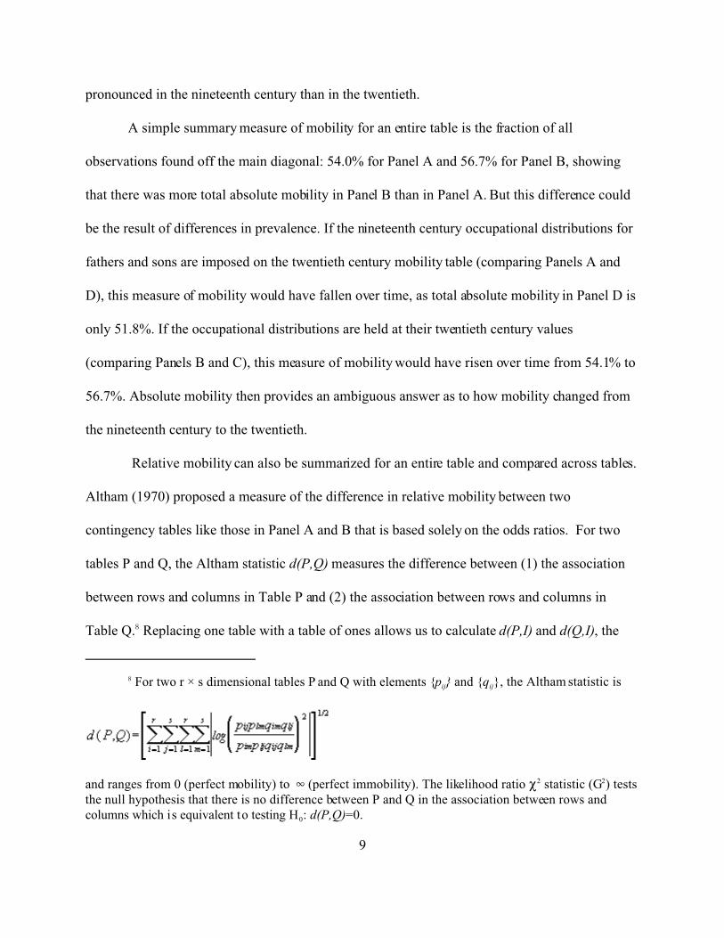
8 For two r × s dimensional tables P and Q with elements {pij} and {qij}, the Altham statistic is

and ranges from 0 (perfect mobility) to 4 (perfect immobility). The likelihood ratio P2 statistic (G2) teststhe null hypothesis that there is no difference between P and Q in the association between rows andcolumns which is equivalent to testing H0: d(P,Q)=0.

9

pronounced in the nineteenth century than in the twentieth.

A simple summary measure of mobility for an entire table is the fraction of all

observations found off the main diagonal: 54.0% for Panel A and 56.7% for Panel B, showing

that there was more total absolute mobility in Panel B than in Panel A. But this difference could

be the result of differences in prevalence. If the nineteenth century occupational distributions for

fathers and sons are imposed on the twentieth century mobility table (comparing Panels A and

D), this measure of mobility would have fallen over time, as total absolute mobility in Panel D is

only 51.8%. If the occupational distributions are held at their twentieth century values

(comparing Panels B and C), this measure of mobility would have risen over time from 54.1% to

56.7%. Absolute mobility then provides an ambiguous answer as to how mobility changed from

the nineteenth century to the twentieth.

Relative mobility can also be summarized for an entire table and compared across tables.

Altham (1970) proposed a measure of the difference in relative mobility between two

contingency tables like those in Panel A and B that is based solely on the odds ratios. For two

tables P and Q, the Altham statistic d(P,Q) measures the difference between (1) the association

between rows and columns in Table P and (2) the association between rows and columns in

Table Q.8 Replacing one table with a table of ones allows us to calculate d(P,I) and d(Q,I), the

10

distance between the association between rows and columns in Table P or Q and the association

between rows and columns in a table in which rows and columns are independent. These distance

measures have likelihood ratio P2 test statistics (G2) to test the null hypothesis that the

associations do not differ, so one can assess whether two tables differ from each other and from

independence (Altham and Ferrie, 2005). If d(P,I) < d(Q,I) and d(P,Q)�0 then Table P has

greater mobility than Table Q (i.e. Table P has an association between rows and columns that is

closer to what we would observe under independence than does Table Q). The Altham statistic is

a pure function of the odds ratios in each table, so it is not affected by differences in the marginal

frequencies.

In Table 1, if we use Panel A for Table P and Panel B for Table Q, we calculate the

following distance measures and test statistics: d(P,I)=14.6, G2=535.4, probability<0.0001;

d(Q,I)=20.8, G2=420.4, probability<0.0001; d(P,Q)=9.1, G2=36.7, probability<0.0001. For both

Panel A and Panel B we can reject the null hypothesis that the occupations of father and sons are

independent. But we can also reject the null hypothesis that the relationship between fathers’ and

sons’ occupations is identical in the two panels. Finally, Panel A (1880-1900) has a relationship

between fathers’ and sons’ occupations that is closer to independence (i.e. displays greater

mobility) than Panel B, so the last twenty years of the nineteenth century had greater relative

mobility in occupations across generations than the twenty years before 1973.

Perhaps the change in the association of occupations from the 1880-1900 period to the

OCG period is an anomaly, a peculiarity of the 1880-1900 sample or the OCG sample. For the

late nineteenth and early twentieth centuries, two additional samples are available: 1860-80 and

1900-20. For the second half of the twentieth century, there are also two other samples. The

11

General Social Survey (GSS) for 1977-1990, conducted by the National Opinion Research

Center, contains information on the respondent’s father when the respondent was age 16. By

selecting individuals who were age 33 to 39 in the survey year and comparing their occupation to

their father’s occupation, it will again be possible to measure intergenerational occupational

mobility over a span of 17 to 23 years. In the National Longitudinal Survey of Youth 1979

Cohort (NLSY79), the respondent’s occupation is available in 1998, and his father’s occupation

is available in 1978, a span of 20 years; individuals age 33-39 in the terminal year are again used.

Figure 1 shows the Altham statistics for each table, along with the p-values, and the

Altham statistic measuring the distance between the association between fathers’ and sons’

occupations in the sample and the association in the 1880-1900 and OCG samples. We can safely

reject the null hypothesis that any of the samples displays intergenerational mobility consistent

with independence of fathers’ and sons’ occupations. But the degree of dependence differs

markedly among them. The nineteenth and early twentieth century tables (1860-80, 1880-1900,

and 1900-20) show approximately the same high degree of mobility, but the twentieth century

tables all show considerably less mobility. All of the pairwise comparisons between the 1880-

1900 table and the twentieth century tables allow us to reject the null hypothesis that the degree

of association is the same in the nineteenth and late twentieth centuries, and in each case mobility

is greater in the nineteenth century than in the late twentieth. Within the twentieth century, it is

not possible to reject the null hypothesis that the degree of association between fathers’ and sons’

occupations is identical for any pairwise comparison. The consistency of the results across these

data sets and time periods suggests that something fundamental changed in the U.S. economy

after the 1900-20 cohort and no later than the 1950/56-1973 cohort and that this change dwarfs

12

any changes in intergenerational mobility since the 1950s.

Mobility in Britain and the United States in the Nineteenth and Twentieth Centuries

Intergenerational occupational mobility in the U.S. clearly “ain’t what it used to be” – at

least in terms of relative mobility. But was it ever “what it used to be”? Were nineteenth and

early twentieth century observers like de Tocqueville, Marx, and Sombart mistaken, or was there

a substantial difference between European and U.S. mobility in the past? Long and Ferrie (2005)

compare intergenerational occupational mobility in the U.S. and Britain in the mid-nineteenth

century using nationally representative longitudinal data. The U.S. data are for 2,005 pairs of

fathers observed in 1850 and their sons (age 43-49) observed in 1880, and the British data are for

3,082 pairs of fathers observed in 1851 and their sons (age 43-49) observed in 1881. Overall

absolute mobility was greater in the U.S. regardless of which country’s distribution of

occupations is used. Specific patterns of mobility also differed substantially. For example, only

51.3 percent of the sons of unskilled fathers in Britain were able to obtain jobs better than

unskilled themselves 30 years later; in the United States, 81.4 percent were able to do so. The

U.S. advantage persists regardless of which country’s marginal frequencies are used (Long and

Ferrie, 2005, pp. 17-22).

Relative mobility was also substantially higher in the U.S. than in Britain over the three

decades after 1850. The Altham statistics for the British 1851-81 data (P) and the U.S. 1850-80

data (Q) are: d(P,I)=23.7, G2=836.6, probability<0.0001; d(Q,I)=11.9, G2=287.2,

probability<0.0001; d(P,Q)=9.1, G2=36.7, probability<0.0001. From these we can conclude that

13

the association between fathers’ and sons’ occupations was a great deal closer to independence

(i.e. exhibited greater mobility) in the U.S. than in Britain, and we can reject at any conventional

significance level the null hypothesis that the associations are equal. As contemporary observers

asserted, the United States had a more fluid occupational structure than Britain. These differences

reflected something more fundamental than differences in the distributions of occupations

between the two economies. The United States was “exceptional” in the mobility it displayed in

the nineteenth century compared to at least one advanced European economy.

British and U.S. mobility in the twentieth century can also be compared using the tools

described above. The Oxford Mobility Study of 1972 provides information on each individual’s

occupation and that of his father when the respondent was 14 years of age that is comparable to

the OCG of 1973. Respondents age 31-37 in the survey year were selected to yield the same

number of years between their father’s occupation and their own as in the OCG (where 33-39

year olds were selected, and their fathers’ occupations were reported when the respondents were

16 years of age). Regardless of which country’s marginal frequencies are used, the U.S. had

roughly 3 percentage points more respondents off the main diagonal (i.e. not in the same

occupations as their fathers). But if the Altham statistics are calculated for Britain (P) and the

U.S. (Q), it is not possible to reject the null hypothesis that relative mobility was the same in both

places: d(P,I)=24.0, G2=168.4, probability<0.0001; d(Q,I)=20.8, G2=420.4, probability<0.0001;

d(P,Q)=7.9, G2=7.5, probability=0.5841 (Long and Ferrie, 2005, pp. 16-17). This confirms the

finding of Erikson and Goldthorpe (1992) that by the second half of the twentieth century,

9 It is not possible at present to calculate the change in mobility within Britain from thenineteenth century to the twentieth, as the historical data used by Long and Ferrie (2005) span thirtyyears and the data from the Oxford Mobility Study span only twenty (to avoid the influence of the GreatDepression). Work in progress will result in a British sample with fathers observed in 1881 and sons in1901 that can be compared directly to both the 1800-1900 U.S. data and the Oxford Mobility Study.

14

relative mobility across generations was no more likely in the U.S. than in Britain.9

Accounting for High U.S. Occupational Mobility Through 1920

The U.S. had more relative occupational mobility across generations through the 1900-

1920 cohort than either Britain in the second half of the nineteenth century or the U.S. in the

second half of the twentieth century. Any attempt to account for these differences must

immediately confront the size of the farm sector in the late nineteenth and early twentieth century

U.S. By 1851, much of the movement out of farming that would ever occur in Britain had already

taken place (the farm sector accounted for less than 5 percent of male employment by 1851). By

1950, farming employed only 12 percent of the adult male labor force in the U.S. In contrast,

throughout the 1850-1920 period, the U.S. farm sector remained large (nearly two thirds of the

adult male labor force in 1850 and more than a third through 1900) and continued to both add

and lose new workers (with net significant losses) (Long and Ferrie, 2005).

Though the Altham statistics used here to measure relative mobility account for

differences both within and across mobility tables in marginal frequencies, there remains the

possibility that the size of the farm sector in the 1850-1920 U.S. nonetheless mattered for relative

mobility. If migration into and out of farming is increasingly selective as the farm sector shrinks,

then those exiting and entering farming in the 1850-1920 U.S. were a less selected population

10 The reduction in the difference between mobility in the historical U.S. and mobility in themodern U.S. when this adjustment is made does not prove that mobility was reduced because of a subtlechange in the selectivity of movement out of and into agriculture as the farm sector shrank. It is possible,for example, that a more important development was a simple change in the costs and benefits of makingthese moves. Perhaps remaining in farming was an increasingly attractive option for the remaining farmsons as subsidy programs instituted in the 1930s stabilized farm incomes, and that the capitalized valueof those benefits made purchasing one’s way into farming a less attractive alternative for those whosefathers were not farmers. Changes in the selectivity of movement from the farm sector on the basis ofunobservable characteristics are examined explicitly in Ferrie (2005a). In either case, it would be unwiseto ignore entirely movement out of and into farming in assessing how mobility evolved, because the farmsector remained so large a fraction of the labor force through the first decades of the twentieth century.

15

than corresponding individuals in late nineteenth century Britain or in the late twentieth century

U.S. If this selectivity takes the form of a reduced willingness to exit or enter the farm sector as it

shrinks, we would expect greater persistence in farming among those whose fathers were farmers

and less entry into farming by those whose fathers were not farmers in Britain after 1851 or in the

U.S. after 1950 than in the U.S. from 1850 to 1920. Long and Ferrie (2005) re-calculated the

Altham statistics after eliminating those who either remained in farming or entered it and find

that this actually widens the gap in mobility between the U.S. and Britain in the nineteenth

century and leaves a much smaller but still statistically significant gap between the late

nineteenth and early twentieth century and the late twentieth century U.S.10

Other explanations for the distinctively high mobility in the late nineteenth and early

twentieth century U.S. can be identified. Economists model intergenerational mobility as the

outcome of a process of investment by parents (perhaps with the assistance of capital markets)

and the state (through its provision of public education) (Grawe and Mulligan, 2004). Where

capital markets function less well or public education is less widely provided, intergenerational

mobility will be lower.

Whether capital markets were better at facilitating intergenerational investments in the

U.S. than in Britain is unknown, so we cannot say whether differential access by parents to

11 Educational access might have still mattered if either: (1) the educational backgroundnecessary to achieve occupational mobility out of one’s father’s occupation was increasing more rapidlythan the level of education being publicly provided; or (2) the distribution of educational access wasbecoming increasingly unequal over time in the U.S. even as the level of education provided was rising.The latter might account for some of the differences between the modern U.S. and countries with moreegalitarian education systems (Canada, Finland).

12 In Democracy in America, de Tocqueville (1835-40 [1862], Book 1, p. 374) observed,“millionsof men are marching at once toward the same horizon; their language, their religion, their manners differ;their object is the same. Fortune has been promised to them somewhere in the west, and to the west theygo to find it.” Mobility was high even in places that had only recently been settled: “I have spoken of theemigration from the older states but how shall I describe that which takes place from the more recent

16

capital produced differential mobility in the nineteenth century . There should be little doubt,

however, that U.S. capital markets by the 1950s were better equipped to help parents invest in

their children’s futures than they had been a century earlier. Yet mobility in the U.S. was greater

from 1850 to 1920 than it was from 1950/56 to 1973. Relatively less access to public education

in Britain than in the U.S. could account for some of the difference in mobility between them in

the nineteenth century – education was less rigorous but more egalitarian in the U.S. than in

Britain in the nineteenth century (Long and Ferrie, 2005, pp. 31-32). But like changes in capital

market access, changes in access to education go in the wrong direction to explain the observed

decline in intergenerational mobility within the U.S.11

A particular form of investment (by either parents or the individuals themselves)

may have still been a source of higher mobility in the late nineteenth and early twentieth

century U.S. Both Schultz (1961) and Becker (1964) suggest viewing migration as an

investment. Internal migration was considerably more frequent in the U.S. at the end of

the nineteenth century than it was in B ritain at the same time or in the U.S . a century later.

When de Tocquev ille surveyed the American economy of the 1830s, he was also

struck by the young nation ’s extremely high rates of geographic mobility. 12 This geographic

ones? Fifty years have scarcely elapsed since Ohio was founded; the greater part of its inhabitants werenot born within its confines; its capital has been built only thirty years, and its territory is still covered byan immense extent of uncultivated fields; yet already the population of Ohio is proceeding westward, andmost of the settlers who descend to the fertile prairies of Illinois are citizens of Ohio. These men left theirfirst country to improve their condition; they quit their second to ameliorate it still more; fortune awaitsthem everywhere, but not happiness” (1835-40 [1862], Book 1, pp. 376-377).

13 The results are similar if other data sets that span ten, 20, or 30 years are used, like the PanelStudy of Income Dynamics or National Longitudinal Survey of Youth 1979 Cohort. No adjustment hasbeen made in these comparisons for the increase in the number of states and counties since the middle ofthe nineteenth century. The NLS does not identify the respondent’s location with sufficient precision tomake such adjustments possible. If new states or counties have been created by subdividing those thatexisted in the nineteenth century, the gap between nineteenth and twentieth century mobility is actuallyunderstated: if modern county boundaries were imposed on historical counties, some intra-county moveswould be reclassified as inter-county moves. If some states or counties were not even part of the settledU.S. in the nineteenth century, the addition of new destinations since the nineteenth century hasexpanded the choice set faced by potential migrants and probably increased measured interstate andinter-county migration; taking account of this would also widen the gap between nineteenth and twentiethcentury migration rates. Only the consolidation of geographic units that existed in the nineteenth century(which occurred rarely) or the addition of new places out of which people were disproportionatelyunlikely to migrate would bias the comparison in the opposite direction and narrow the gap betweenhistorical and modern migration rates.

17

mobility, too, became a facet of “American exceptionalism.” The U.S. was characterized by

greater residential mobility than Britain in the second half of the nineteenth century. Inter-county

moves were made by nearly two-thirds of U.S. men over 30 years, but were made by only a

quarter of British men (counties being roughly the same size on average in both countries). Most

moves in Britain were short distance (median=5 miles, mean=24 miles), while in the United

States, distances were longer (median=36 miles, mean=213 miles) with more than a third over

100 miles compared to only 6 percent in Britain. Was there also a decline in physical mobility in

the U.S. over time that parallels the decline in occupational mobility across generations in Figure

1?

Table 2 shows rates of inter-county and interstate migration for young men and older men

over a decade for three nineteenth century samples and the National Longitudinal Survey (NLS)

cohorts of Young Men and Older Men in the twentieth century.13 Except for the decade of the

14 Kim constructs a measure of the concentration of economic activity across sectors by region atthe one-digit SIC level.

18

Civil War, inter-county and interstate migration rates were extraordinarily high before 1900. By

the twentieth century, there is a drop in inter-county migration and an even sharper drop in

interstate migration. The high rates of mobility in the 1850s and 1870s are remarkable at a time

when the cost of migration (both the direct transportation cost and the cost of acquiring

information about alternative locations) must have been considerably higher than today.

Are declining rates of geographic mobility related to the changes documented above in

the association between the occupations of fathers and sons? Kim (1998) finds that regional

specialization increased through 1880, fell slightly through 1910, and then fell dramatically

throughout the rest of the twentieth century.14 This suggests that through the first decades of the

twentieth century, even as the frontier was closing and movement into farming was less

frequently a route to economic advancement, substantial differences across locations in the

predominant economic activities left another route to advancement: migration to places that were

growing more rapidly than others. Opportunities for “locational arbitrage” may have allowed

many of those whose prospects were poor at their original location to seek out promising

destinations. By the early decades of the twentieth century, fewer such arbitrage opportunities

remained, and migration distances fell as movement was redirected away from distant, rapidly-

growing places to adjacent cities and towns which could often be reached by crossing a county

boundary but without crossing a state boundary, accounting for the sharper decline in interstate

migration than in inter-county migration.

Were those who moved physically also more mobile occupationally? For the late

nineteenth and early twentieth century cohorts, it is possible to calculate separate Altham

15 For non-migrants (P) and migrants (Q), the Altham statistics for each cohort are:

d(P,I) G2 prob d(Q,I) G2 prob d(P,Q) G2 prob1860-80 20.5 372.6 0.0001 8.0 99.4 0.0001 13.5 95.2 0.00011880-1900 21.0 502.5 0.0001 11.1 147.1 0.0001 12.2 90.2 0.00011900-20 22.9 414.4 0.0001 10.3 115.7 0.0001 14.1 78.1 0.0001

It would be unwise to describe geographic mobility as the cause of higher mobility, however, as if it werea randomly-assigned treatment applied to an entire population. The migration decision was no doubtmade with an eye toward the individual’s future prospects, so the population of migrants may have beenselected for those who expected to derive the greatest benefit from changing locations. The evidenceoffered here is intended to be no more than suggestive. The selectivity of migration from rural to urbanplaces and to the western frontier is examined in Ferrie (2005a and 2005b).

19

statistics to measure relative occupational mobility for two groups: (1) those who changed their

county of residence over twenty years and (2) those who remained in the same county. In each

case, the Altham statistic was at least twice as great (mobility was lower) for those who remained

in the same county. For all three cohorts – 1860-80, 1880-1900, and 1900-20 – it is possible to

reject the null hypothesis that the relationship between fathers’ and sons’ occupations was

identical for movers and non-movers.15

As the importance of geographic mobility as an avenue to economic advancement

diminished, the importance of education has risen over the twentieth century. Goldin (1994)

documents the changes in American high school education taking place between 1910 and the

early 1930s: an increased emphasis on practical, job-relevant skills and vocational training, as

well as much higher high school graduation rates. Research on recent trends in mobility has

emphasized the role of family investment in education in fostering intergenerational mobility (in

incomes) as the returns to education have risen (Mayer and Loppo, 2001). Though families in the

early twentieth century no doubt increased investment in their children’s human capital as

geographic mobility became less viable as a route to occupational mobility, the benefits that

education provides are quite different from the benefits of geographic mobility. For a young

20

adult, education is much less a choice variable than is location. Education choices may be more

often subject to a binding budget constraint than choice of location. And education depends on

the wisdom of the previous generation in choosing the proper investment level. A change from

geographic mobility to educational investment as the avenue to intergenerational mobility in the

twentieth century may have left families with fewer options than in the nineteenth century.

Conclusion

Nineteenth-century observers were right: the United States was in fact more mobile both

socially and physically than other places, and this remarkable fluidity persisted at least through

the 1920s. However, that distinctiveness had diminished by the 1950s. It remains to be seen why

mobility diminished when it did. Though Marx predicted that the closing of the frontier would

reduce American mobility to European levels, inter-generational mobility remained common

through the first two decades of the twentieth century, decades after the 1890 closing of the

frontier. Promising avenues of future research in explaining the mobility transition are the

changing roles of geographic mobility and education, the rise of internal labor markets in the

1920s that placed a premium on remaining with the same firm and foreclosed some inter-firm

mobility as a route to upward occupational movement, and the birth of the American welfare

state and corresponding reduction in the need to seek work in new places in response to negative

shocks to local economies.

21

Acknowledgments

The National Science Foundation provided financial support for the collection of the

1850-60 and 1860-70 samples (Grant No. 9309689 and Grant No. 9730243). Extremely useful

comments were provided by Claudia Goldin, James Hines, Robert Margo, Enrico Moretti,

Richard Sutch, Timothy Taylor, Michael Waldman, and participants at the 2004 ASSA Meetings,

the 2004 NBER/DAE Summer Institute, the 2004 Social Science History Association Meetings,

the 2004 All-UC Economic History Conference, and seminars at Northwestern, McGill,

Michigan, Queens, and the Ecole Normale Supérieure (Paris).

22

A. 1880-1900 Father’s OccupationUsing 1880-1900 Occupational Dist. (Column Percent)

White Skilled/Son’s Occupation Collar Farmer Semi-Skilled Unskilled Obs.

White Collar 56.9 16.6 26.6 19.0 589.0 Farmer 9.5 46.6 10.8 16.0 786.0Skilled/Semi-Skilled 21.6 19.6 46.9 35.4 684.0Unskilled 12.0 17.2 15.6 29.5 440.0Obs. 283.0 1411.0 537.0 268.0 2499.0

B. 1950/1956-1973 Father’s OccupationUsing 1950/1956-1973 Occupational Dist. (Column Percent)

White Skilled/Son’s Occupation Collar Farmer Semi-Skilled Unskilled Obs.

White Collar 71.4 31.9 43.6 35.1 1442.0Farmer 0.4 13.5 0.6 1.1 76.0Skilled/Semi-Skilled 22.3 42.8 46.6 50.5 1191.0Unskilled 5.9 11.8 9.3 13.3 279.0Obs. 833.0 451.0 1237.0 467.0 2988.0

C. 1880-1900 Father’s OccupationUsing 1950/1956-1973 Occupational Dist. (Column Percent)

White Skilled/Son’s Occupation Collar Farmer Semi-Skilled Unskilled Obs.White Collar 73.3 41.0 39.5 33.8 1442.0Farmer 1.0 9.2 1.3 2.3 76.0Skilled/Semi-Skilled 20.6 35.9 51.7 46.8 1191.0Unskilled 5.1 13.9 7.6 17.1 279.0Obs. 833.0 451.0 1237.0 467.0 2988.0

D. 1950/1956-1973 Father’s OccupationUsing 1880-1900 Occupational Dist. (Column Percent)

White Skilled/Son’s Occupation Collar Farmer Semi-Skilled Unskilled Obs.

White Collar 59.7 12.8 32.7 23.9 589.0Farmer 2.9 52.2 4.1 7.0 786.0Skilled/Semi-Skilled 22.2 20.4 41.6 41.0 684.0Unskilled 15.2 14.6 21.6 28.0 440.0Obs. 283.0 1411.0 537.0 268.0 2499.0

Table 1. Intergenerational Occupational Mobility, 1880-1900 and 1950/1956-1973 (White, Native-Born Males Age 33-39 in Terminal Year).

23

Figure 1. Altham Statistics Measuring Distance from Independence, fromAssociation in 1880-1900, and from Association in OCG (1973), WhiteNative-Born Males Age 33-39 in Terminal Year. Source: See text.

Inter-County Interstate

N Migrants MigrantsAge 20-29 in initial year 1850-60 (Ferrie sample) 1,158 49.5% 26.2% 1860-70 (Ferrie sample) 466 38.2 17.8 1870-80 (Ferrie sample) 3,602 54.7 30.1 1971-81 (NLS Young Men) 1,866 41.7 21.5

Age 45-59 in initial year 1850-60 (Ferrie sample) 529 21.2 10.6 1860-70 (Ferrie sample) 347 20.5 8.4 1870-80 (Ferrie sample) 2,124 34.5 21.5 1966-76 (NLS Mature Men) 3,503 16.0 8.1

Table 2. Geographic Mobility (White, Native-Born Males Age 20-29 and 45-59 in Initial Year).

24

References

Alberto Alesina, Rafael Di Tella, Robert MacCulloch. 2001. “Inequality and Happiness: AreEuropeans and Americans Different?” NBER Working Paper No. w8198.

Altham, P.M. 1970. “The Measurement of Association of Rows and Columns for an r × sContingency Table.” Journal of the Royal Statistical Society, Series B, 32, pp. 63-73.

Altham, P.M., and J.P. Ferrie. 2005. “Contingency Table Comparisons.” Working Paper,Northwestern University Department of Economics.

Becker, Gary. 1964. Human Capital. New York: National Bureau of Economic Research.Bjorklund, Anders, and Markus Jantti. 1997. “Intergenerational Income Mobility in Sweden

Compared to the United States.” The American Economic Review, 87: 5, December, pp.1009-1018.

Erikson, Robert, and John H. Goldthorpe. 1992. The Constant Flux: A Study of Class Mobility inIndustrial Societies. New York; Oxford University Press.

Featherman, David L., and Robert M. Hauser. 1978. Opportunity and Change (New York:Academic Press).

Ferrie, Joseph. 2004. “Longitudinal Data for the Analysis of Economic Mobility in theNineteenth Century U.S.” Working Paper, Northwestern University Department ofEconomics.

Ferrie, Joseph. 2005a. “How Ya Gonna Keep ’Em Down on the Farm [When They’ve SeenSchenectady]? Rural to Urban Migration in the Nineteenth Century U.S.” Working Paper,Northwestern University Department of Economics.

Ferrie, Joseph. 2005b. “Migration to the Frontier in Ante-Bellum America: A Re-Evaluation ofTurner’s ‘Safety Valve’ Hypothesis.” Working Paper, Northwestern UniversityDepartment of Economics.

Ganzeboom, Harry, Pauil M. De Graaf, Donald J. Treiman and Jan De Leeuw. 1992. “AStandard International Socio-Economic Index of Occupational Status.” Social ScienceResearch 21, pp. 1–56.

Goldin, Claudia. 1994. “How America Graduated from High School, 1910 to 1960.” NBERWorking Paper No. H0057 (June).

Hout, Michael and Robert M Hauser. 1992. “Symmetry and Hierarchy in Social Mobility: aMethodological Analysis of the CASMIN Model of Class Mobility.” EuropeanSociological Review 8: 3, pp. 239–266.

Kim, Sukkoo. 1998. “Economic Integration and Convergence: U.S. Regions, 1840-1987.”Journal of Economic History, 58: 3 (September), pp. 659-683.

Long, Jason, and Joseph Ferrie. 2005. “A Tale of Two Labor Markets: IntergenerationalOccupational Mobility in Britain and the U.S. Since 1850.” NBER Working Paper No.w11253 (March).

Marx, Karl. 1865 [2001]. Value, Prices, and Profits (London: Electric Book Company).Mayer, Susan E., and Leonard Lopoo. 2001. “Has the Intergenerational Transmission of

Economic Status Changed?” University of Chicago, Harris School of Public Policyworking paper.

Mosteller, Frederick. 1968. “Association and Estimation in Contingency Tables.” Journal of theAmerican Statistical Association, 63, pp. 1-28.

25

Piketty, Thomas. 1995. “Social Mobility and Redistributive Politics.” Quarterly Journal ofEconomics, Vol. 110, No. 3. (Aug., 1995), pp. 551-584.

Schultz, Theodore W. 1961. “Investment in Human Capital.” American Economic Review, 51,pp. 1-17.

Shafer, Byron E. 1999. “American Exceptionalism.” Annual Review of Political Science 2. pp.445-463.

Solon, Gary. 2002. “Cross-Country Differences in Intergenerational Earnings Mobility.” Journalof Economic Perspectives. Summer, 16: 3, pp. 59-66.

Sombart, Werner 1906 [1976]. Why Is There No Socialism in America, translated by PatriciaHocking and C.T. Husbands (New York: M.E. Sharpe).

Sorensen, Jesper B. 1992. “Locating Class Cleavages in Inter-Generational Mobility:Crossnational Commonalities and Variations in Mobility Patterns.” EuropeanSociological Review 8: 3, pp. 267–281.

Tocqueville, Alexis de. 1835-40 [1862]. Democracy in America. Translated by Henry Reeve(Cambridge: Sever and Francis).

Winthrop, John. 1630 [1995]. “A Model of Christian Charity.” Norton Anthology of AmericanLiterature. Shorter Fourth Edition (New York: W.W. Norton), pp. 101-112.