EtC - NBER

N DRKtG PAPfl SRI

PLAIND FISL FCIIcIFS ND INflTIfl DEVEEOPD3 IRIES

Sebastian Edwards

Guido Thbellini

Working Paper No. 3493

'ICL 3RENJ OF EtC RSEN-I1050 Massadiusetts Avenue

n'bri&e, Wi 02138tcber 1990

This paper is part of NEER's reseaith prcxram in International Stxlies. ?nycpinions expressed are those of the authors ar rxt those of the National3reau of Eczxtnic Researth.

NBER Workirg Paper #3493Cctcber 1990

EPIAINfl FISL IOLIcES flflTIc1fli VDPfl cXXNIRIES

In this paper we investigate erririca1ly the determinants of inflation,

seigniorage an fiscal deficits in develcpin xxntries. We first test the

cçtixnal tation theory of inflation for a grip of 21 I1Xs. We fiixl that

the inp1icaticz- of this theory is rejected for all t1e czxintries. We then

pro to inplnt a rvther of tests based on the i political xziyaproadi to ]nacroecxrxillic policies: we deal with sai of the inp1icaticz of

a credibility az repitation nx3e1, ar of a strataic goverrmEnt behavior

ne1. We firx that the data supports the nxst isportant praiicticr of the

political uuny view of fiscal policy. C*.ir asures of political

instability ar political polarization play an inportant role in explainirg

cross cx*mtxy differezres in seigniorage, inflation, verrznt borrcizg arfiscal deficits. We eni by discussirq directions for futere researth.

Sebastian Edwards Guido TabelliniDeparnt of Econatiics Departnent of Ecrn*nicsUA UA405 Hilgard Ave. 405 Hilgard Ave.Los Arieles, CA 90024 Los Are1es, CA 90024

1

I. Introduction

In recent years we have witnessed some important developments in the

analysis of fiscal policies. Dynamic models of taxation in closed and open

economies have become part of the economists' tool box; issues regarding

Ricardian neutrality, or lack of it, are topics of daily discussions. We

now have (or we think we have) a clear idea of what will happen to the key

macro variables such as the price level, interest rates, the real exchange

rate, wages, unemployment, and so on when there are different fiscal shocks.

However, moderrt economic analyses have until recently failed to fully

address the key question of ii determines a country's fiscal policy. In a

phrase, the problem is that economists most of the time treat the

policymaker as a machine that can be programmed. Once the right policy has

been singled out, the economist's task is over: it is up to the policy-

maker-machine to implement it. This is a serious limitation of the

traditional approach to the theory of economic policy. Policyrnakers, just

like every other economic agent, behave purposefully and respond to

incentives and constraints. There is little doubt that the Argentinian

authorities, for example, have a fairly clear idea of what are the consequ-

ences of accelerating the rate of growth of domestic credit on inflation,

the balance of payments, capital flight and so on. Still, even knowing

these consequences they chose to go ahead. Why? To answer this question,

one needs to formulate a positive theory of how policymakers behave.

A small but growing body of literature has recently pursued this

positive approach to the theory of monetary and fiscal policy, building on

insights developed from game theory and theory of the public choice. Most

of this literature, however, has been theoretical and has dealt almost

exclusively with the advanced nations.

2

In this paper we do two things: first we review this positive approach

to economic policy, analyzing its applicability to the cue of the develop-

ing countries. In doing this broad review, we extend some models, propose

new theories and report some new results obtained during the course of our

own research. Second, we provide new empirical evidence on the fiscal and

monetary behavior of developing countries. This empirical investigation

yields a general lesson: political institutions and political incentives

are central determinants of observed economic policies.2

The paper is organized in two parts. The first reviews the recent

literature on the theory of inflation and investigates the empirical

evidence on time series and cross-country data. We find that this evidence

is inconsistent with the conclusions of the theory of optimal taxation. We

also find that inflation is very strongly related to different measures of

political instability. The second part of the paper reviews the theory and

the evidence on government budget deficits. Again, the central finding is

that more unstable political systems tend to be associated with larger

government borrowing. The paper ends with a brief concluding section that

proposes new directions for future research.

II. Inflation

In this section we systematically analyze the theory and evidence on

inflation for a large group of developing countries. We start by providing

a broad analysis of the data and then move to test alternative theories on

the long run determinants of inflation.

11.1 The Inflation Tax

Table 1 contains data on inflation and seignorage for 52 developing

countries for different subperiods 1963 and l987. For each of them we have

3

computed the average rate of inflation of the consumer price index and the

average revenue from the inflation tax, expressed as a percentage of GDP.

For every year this revenue was calculated as:

R_!! (1)

where w is the inflation rate, m is the monetary base and y is GDP.4

The last row of the table shows the standard deviation of these variables

across countries for each subperiod. All the data were obtained from the

most recent IFS tape.5

These figures strikingly illustrate a wide variability in the inflation

tax, both across countries and across time. First, in most countries there

is an important increase in the rate of the inflation tax in the late 1970s

and early 1980s. Second, the cross country variability is remarkable, both

regarding the rates as well as revenues. For the period 1963-73 the ratio

of higher to lower rate of the inflation tax was 41 times. For 1983-87 this

ratio had climbed to more than one thousand times!6 Similarly, between

these two subperiods the standard deviation of inflation across countries

increased by more than eight times. Third, in a number of countries,

increases in the rate of inflation resulted in a reduction of the inflation

tax revenue. Examples of this phenomenon are Ghana (73-78 vs. 78-83);

Ma].awj (73-78 vs. 78-83); Zaire (73-78 vs. 78-83); and Chile (63-73 vs. 73-

78). The extent of this phenomenon is probably greater than what is

apparent from Table 1, since, as argued by Tanzi (1977) and Olivera (1967),

inflation may reduce the base of other taxes - - either through encouraging

the underground economy or because of collection lags. Fourth, contrary to

the popular belief, we observe very wide differences in behavior within

Latin America. For example, in every period we can find some Latin American

4

countries with a very low rate of inflation; in fact, lower than the average

of the Asian nations. This is an important finding since it provides a

counterexample to the popular 'cultural theory of inflation differentials

across countries. According to that view cultural reasons explain why Latin

America is fiscally irresponsible. Our data, however, show that Latin

America is far from being a homogeneous group. Thus, any good theory that

attempts to explain the determinants of fiscal policy and the inflation tax

should be capable of explaining the different behavior encountered within

the Latin American region.

Figures 1 through 3 depict the relationship between the rate of

inflation and the log of the inflation tax revenue for a group of selected

countries. These diagrams suggest that in most of these countries there is

indeed a Laffer curve type relation between the rate of inflation and the

inflation tax revenue. Moreover, they also suggest that at one point or

another some of these countries may indeed have been on the 'wrong sIde' of

this curve.

To sum up, then, the evidence presented here not only shows a wide

variety of cross-country experiences with the inflation tax, but also

suggest that the Inflation tax rate sometimes exceeds the rate that would

maximize revenues from this source. In the rest of this section we

investigate empirically a number of possible explanations for these observed

cross country differentials in inflation. We start by analyzing theories of

dynamical optimal taxation, and then proceed to investigate models that

focus on credibility constraints and political incentives.

11.2 The Theory of Optimal Taxation

A first important question is whether the observed pattern of the

inflation tax can be explained as the optimal government response to a

5

politically desired path of public spending. The modern theory of public

finance lends some support to this view. In the presence of tax evasion, or

if there are tax collection costs in administering other tax instruments, it

is optimal for the government to rely on the inflation tax (Aizenman (1987),

Faig (1988) and Kimbrough (1986)). Clearly, tax evasion and tax collection

costs are common-place in developing countries. Hence, according to the

theory of optimal taxation we should expect developing countries to rely on

the inflation tax as a source of revenue, the more so the larger are tax

collection costs and the larger is tax evasion.

Suppose that the government can use the inflation tax (w) and other

tax rates on output (r) to finance its expenditures. Both taxes are

distortionary and impose a welfare cost that is increasing on their rate.

The cost of the output tax rate is f(r) while that of the inflation tax is

h(s. Mankiw (1987) shows that in these circumstances the optimal tax

policy implies:

— kf?(i.t) (1)

where k is a parameter of the money demand function. Thus, at the optimum

the marginal cost of each tax has to be equated in every period. This

implies that as government expenditure changes, inflation and non-inflation

tax rates move together. Mankiw (1987) tested this implication using U.S.

data for 1951-82 and found a positive relationship between inflation and the

average tax rate. He interprets this finding as providing support for the

theory of optimal taxation as a positive theory of policy behavior.

More recently a number of authors have extended ?(ankiw's work both theor-

etically and empirically. Vittorio Grilli (1989) has pointed out that

Mankiw's tests fail some important implications of the theory, including the

6

fact that seignorage and income taxes should have a unit root and should be

cointegrated. His results for 10 European nations are mixed; in only some

countries seignorage has behaved as predicted by the optimal taxation theory.7

Poterba and Rotemberg (1990) aAke a distinction between governments

that can commit to a course of action and those that cannot. In their

model, in the commitment case inflation and taxes will be positively cor-

related, while in the absence of commitment inflation will be a positive

function of both taxes and total government liabilities as a percentage of

GNP. They estimate both versions of the model, using OLS and instrumental

variables, on time series data for five countries -. France, Germany, Japan,

the U.K., and the U.S. -- and conclude that for these nations the evidence

does not provide a generalized support to the optimal taxation view of

inflation. As in previous cases this theory only seems to hold for the case

of thq United States.

This type of work has recently been criticized on two counts. On one

hand, Dornbusch (1989) has pointed out that while the theory is based on

marginal tax rates, most (if not all) empirical tests have used computed

average rates. On the other hand, Judd (1990) points out that the welfare

costs of the inflation tax should be related to exoected inflation, rather

than to actual inflation. Thus, according to the theory of optimal taxa-

tion, tax rates and expected (but not necessarily actual) inflation should

move in the same direction. Moreover, any innovation in government spending

or the tax bases should result in unexpected changes in actual inflation.

While Judd's distinction between expected and unexpected inflation is

important, his argument tat only expected inflation has welfare costs is

not generally valid (for instance, it relies on the government neglecting

the redistributions within the private sector that are brought about by

7

unexpected inflation or deflation). We return to this point below.

11.3 Testing Theories of Ovtimal Taxation for LDCs

As Grilli (1989), among others, has pointed out, an important implica-

tion of the optimal taxation hypothesis is that both the inflation rate and

the tax rate should have a unit root. Table 2 contains augmented Dickey-

Fuller unit root tests for these two variables for 21 countries with long

enough annual time series.8 In all cases, except inflation In India, the

unit root hypothesis is not rejected. However, a potential limitation of

these tests is the very short length of the time series. Indeed, it is well

known that as the number of observations is reduced the power of the augment-

ed Dickey-Fuller test greatly diminishes. For the case of inflation we can

get around this problem by using quarterly data.9 This is done in Table 3 we

report augmented Dickey-Fuller tests for a larger group of 44 countries. As

can be seen, as in the case of Table 2, for the vast majority of the count-

ries the hypothesis that inflation follows a unit root cannot be rejected.

These results are not, however, sufficient evidence in favor of the

optimal taxation theory of inflation. Indeed, a unit root is a necessary

but not sufficient condition of the optimal taxation theory. In order to

provide strong support for this theory It is required that seignorage is

positively correlated with the rate of the income tax. To investigate this

aspect of the optimal taxation theory for the LDCs we estimated a Mankiw

type regression for the countries in Table 2:

MNF — a0 +a1 LTAX + (2)

where INF is the yearly rate of Inflation and TAX is the (implicit) yearly

rate of tax on output computed, as In Table 2 and in Mankiw (1987), as the

ratio of tax revenues to GDP. If the theory of optimal taxation presented

8

above is correct, would be significantly positive. Moreover, Mankiw

argues that it should be roughly equal to one)° The results obtained from

these regressions using both OLS and instrumental variables are reported in

Table 411 As can be seen, for most countries these results strongly reject

the hypothesis that there is a positive relation between the output tax rate

and the inflation tax rate. Other preliminary work, not reported here for

reasons of space, indicates that at the core of this rejection lies a strik-

ing stylized fact: the inflation tax often behaves as a residual source of

government revenue. It goes up when spending increases or when other

sources of revenue fall. There are a number of possible explanations for

12these results. But the simplest, and the one that we explore in the rest

of this paper, is that the theory of optimal taxation does not apply to

these countries; the alternative view that we analyze is the political

economy one.

11.4 Credibility and Inflation

Perhaps the simplest explanation of why governments do not behave

according to the theory of optimal taxation is that they lack credibility.

Since the work of Calvo (1978) and Kydland-Prescott (1977), it is well known

that the optimal inflation tax is tine-inconsistent in the absence of

binding policy commitments. In a credible (or tine consistent) equilibrium

with policy discretion, the government relies too much on the inflation tax.

Moreover, in any such equilibrium, the inflation tax is a residual: any

change in government spending is reflected one-for-one in higher inflation,

with little or no effect on other sources of revenue (see Persson-Tabellini

(1990)). Finally, as remarked in Calvo (1978) and more recently in Persson-

Tabellini (1990), policy discretion generally results in a multiplicity of

equilibria. Hence, any specific equilibrium is intrinsically fragi1e".

9

This may result in sudden bursts of accelerating inflation, accompanied by

devaluation. and speculative attacks on fixed exchange rate regimes.

These qualitative properties of models with policy discretion are

remarkably consistent with the empirical evidence reported in Subsection

11.3 on optimal taxation and with the evidence on devaluation crises (see

Edwards 1989). Moreover, they are robust: for instance, they would also

result (with some qualifications) from models in which even actual (and not

just expected) inflation is distorting or undesirable.

Recent developments of the literature on credibility have pointed out

that reputation can be a substitute for commitments. This suggests an obvi-

ous line of empirical attack: to try to explain differences in the observed

rates of inflation in various countries as due to differences in the

strength of reputational incentives in each country. Persson and Tabellini

(1990) have formulated a simple model of reputation with enough institution-

al content to yield positive predictions. The model is built on three

central assumptions: (i) unexpected policy actions disrupt the system of

expectations of private economic agents (for instance, leading to higier

expected inflation and to higher nominal wages); (ii) this disruption of

economic expectations has negative welfare effects on voters; (iii) elect-

ing a new government stabilizes expectations and, thus, reduces the extent

of the disruption. This model of reputation points out that the government

incentive to maintain its reputation has an important political dimension:

the cost of policy surprises is that the government is less likely to be

reappointed in office. The citizens realize that reappointing a government

who created policy surprises means higher expected inflation in the future,

and hence lover social welfare. Thus, they are less likely to reappoint it.

If the government cares about being in office, this punishment creates

10

incentives not to engage in policy surprises.

This model of reputation yields two central positive implications.

First, the equilibrium inflation rate is higher the more the citizens

disagree about which government they prefer to hold office. In other words,

more polarized and •heterogeneous societies encounter greater difficulty in

enforcing low inflation through reputational forces. Second, the equilib-

rium inflation rate tends to be higher the more unlikely it is that the

government currently in office will be reappointed. In other words, reputa-

tion is not very effective if the government is weak. Intuitively, the

threat of being thrown out of office becomes less powerful if society is very

polarized, or if the government is already weak. In the last case, this

occurs because a weak government has little to lose (since it is already

likely to be thrown out of office anyway). In the former case, it occurs

because if society is very polarized, citizens are unwilling to switch party

and punish a government because it just created policy surprises.

Table 5 reports some preliminary evidence consistent with these two

implications. This table reports the results of estimating an OLS regres-

sion of average inflation against various measures of political instability

and polarization, on cross-country data. Estimation is by seemingly

unrelated regressions (StiR). In the first specification of Table 5 (Panel

A), political instability is measured as the frequency of (regular and

irregular) government changes during the relevant time interval. In the

second specification we distinguish between the frequency of regular

government changes and the frequency of military coups. Since the latter

mode of government transfer is likely to involve a more radical change in

the ideology of the government, the frequency of coups is a measure of both

instability and polarization of the political system. The results are

11

striking: the estimated coefficients are almost always positive and often

highly significant. The same results are obtained if we replace the actual

frequency of government change with a measure of the expected probability of

a government change. estimated from a probit model. This alternative meas-

ure of political instability, used for the first time in Cukierisan, Edwards

and Tabellini (1989), is described in more detail in Section 11.5 below.

It should be noticed that the evidence reported in Table 5 could have

several other explanations, some of which will be addressed in later

sections of the paper. One of such explanations, however, is the one

summarized in the previous pages: more unstable and polarized countries

have greater credibility problems, because the reputational incentives of a

government are weaker.3

11.5 Long Run Seignoraze. Tax Reforms and Political Instability

In the previous subsections we presented empirical results based on a

number of alternative approaches to analyze the time series properties of

inflation and government debt in developing countries. We now turn to the

question of how to compare the long-run properties of these same variables

across countries.

According to the theory of optimal taxation discussed in Section 11.2,

the long-run characteristics of inflation and debt depend on the cost of

administering tax collection. High tax collection costs and tax evasion

force developing countries to rely on highly inefficient forms of taxation,

such as inflation or trade related taxes. This explanation raises a natural

question. Why do some countries have higher tax collection costs and higher

tax evasion than others? In the traditional development literature, this

question is answered by arguing that the taxing capacity of a country Is

technologically constrained by its stage of development and by the structure

12

of its economy: a country with a large agricultural sector, for instance,

is more susceptible to tax evasion than a country with a large corporate

manufacturing industry. Cukierman, Edwards and Tabellini (1989) have

explored an alternative answer to this question. Namely, that the evolution

of the tax system of a country depends on the features of its political

system, and not just on those of its economy.

Their central idea can be stated as follows. An inefficient tax system

(i.e., one that facilitates tax evasion and imposes high tax collection

costs) acts as a constraint on the revenue collecting capacities of the

government. This constraint may be welcomed by those who disagree with the

goals pursued by the current government. In particular, a government (or a

legislative majority) may deliberately refrain from reforming a tax system,

for fear that a more efficient tax apparatus will be used in the future to

carry out spending or redistributive programs that the current government

disapproves of. Of course, this is more likely to happen in countries with

more unstable and polarized political systems. Hence, according to this

model, more unstable and polarized political systems rely on inefficient

taxes, such as seignorage and trade taxes, to a greater extent than more

stable and homogeneous countries.

Cuikerman, Edwards, Tabellini (CET) (1989) confront the data by

estimating an equation of the following form for a group of 79 countries:

y — f(x,p)

where y — fraction of total revenue collected through seignorage

x — vector of variables measuring the available tax bases (such as

size of the manufacturing1 mining, and agricultural sectors,

size of imports and exports, per capita income, etc. -. see

13

Tait, Cratz and Eichengreen (1979)).

p — vector of political variables measuring the political

instability and/or polarization.

The question to be posed to the data concerns the role and explanatory power

of the political variables, once the economic variables relating to the stage

of development and the structure of the economy are being controlled for.

Perhaps the most difficult problem faced in this type of empirical analysis

in finding empirical counterparts for the analytical constructs 'political

instability' and 'political polarization.' With respect to the former CET

use an estimated cross-country probit equation to compute an index of the

probability of government change for a particular country in any given year.

This probit equation regresses instances of actual government changes against

political variables (riots, repressions, and so on), economic variables

(consumption growth, inflation, income per capita) and institutional

variables. With respect to polarization they use two alternative proxies:

(i) frequency of coup attempts; (ii) an index of income distribution. This

indicator differs from the index of actual frequency of government change

used in Table 5, in that it provides a measure of the expected probability of

government change, derived from broad cross country evidence.

In addition to the political instability index, in their regression

analysis of seignorage CET included the following structural variables:

(a) share of agriculture in GDP. Its sign is expected to be negative;

since it is relatively costly to tax agriculture, governments with a large

agricultural sector will tend to rely more heavily on taxes with low

administering cost, such as seignorage and trade taxes; (b) share of

mining and manufacturing on GDP. Its sign is expected to be negative, also

for cost effective reasons; (c) foreign trade share on GDP. Its sign is

14

expected to be positive, since in an open economy it is easier to tax

international trade; (d) CDP per capita, whose sign is expected to be

negative. More advanced nations are able to implement more sophisticated

and efficient tax systems, and thus will tend to rely less heavily on easy

to collect but highly distortive taxes such as seignorage; and (e) urban-

ization ratio, whose sign is expected to be negative. The reason is that it

is relatively easier to tax the urban population than the rural population.

For a sample of 58 developing nations, CET obtained the following

results from an OLS regression (standard errors in parentheses) of

seignorage on political instability and other structural variables:14

Seignorage — - 0.020 + 0.0021 Share of Agriculture in CDP(0.032) (0.0005)

- 0.0431 Openness - 0.44E-5 GDP per Capita(0.0182) (0.024E-5)

+ 0.0019 Urbanization + 0.1583 Political Instability Index(0.0004) (0.0539)

— 0.448

S.E. — 0.049

These results are very suggestive. Not only does the regression explain

a high percentage of the cross-country variability of seigniorage, but all

variables have the expected sign.15 Moreover, the coefficient of the

political instability index is highly significant. When a broader group of

countries that includes industrialized nations was considered, the results

were similar to those reported here. All in all, then, the CET results

provide broad support for the hypothesis that, even after controlling for

other structural variables, political instability plays an important role in

explaining long-run cross-country differentials in inflation.

15

An interesting empirical extension of the CET model of strategic

political behavior and tax reform is that the use of other inefficient

taxes such as import tariffs and export taxes, should also be positively

related to political instability. That is, just as in the case of

seignorage, after controlling for other structural variables, political

instability and the reliance on taxes on foreign trade should be positively

related in cross-country data.

This conjecture is tested in Table 6 on a cross section of

industrialized and developing countries. The dependent variable is the ratio

of trade taxes as a percentage of government revenues obtained from the IMF

Government Finance Statistics. The structural variables are the same as

those discussed above and used by CET in their seignorage investigation. The

political variables are the estimated political instability index described

before, the observed frequency of regular (democratic) government change and

the frequency of coups. In addition, we incorporated a dummy variable for

industrialized nations and one for Latin American countries.

The results in Table 6 are mixed. First the coefficients for the

structural variables, with the exception of CDP per capita in two of the

regressions, have the expected sign, and some of them are highly significant.

Second, in both regressions where it is included, the political instability

index has the expected positive sign; however, in neither was its coefficient

significant. Third, when the frequency of coups is added, as a proxy for

political polarization, its coefficient is positive as expected but, again,

it is not significant at conventional levels. Moreover, in this last

regression, the frequency of regular government transfers has the wrong sign.

These less than fully satisfactory results on trade taxes contrast with

the highly supportive results obtained by CET (1989) for seigniorage

16

collection. A possible explanation for these differences in the results is

that, contrary to the case of seigniorage, trade taxes also piay an import-

ant role in determining the productive structur. of a country. Indeed, by

providing protection to certain sectors these types of taxes shape the

incentive structure of the economy. An additional difference between

seignorage and trade taxes that can be affecting these results is that,

while seignorage can be manipulated through administrative decisions,

changes in trade taxes usually require congressional approval. Once these

elements are incorporated into the analysis, the straightforward implication

of the CET model of strategic government behavior is not any longer

applicable to trade taxes.

The empirical evidence discussed in this section can be summarized as

follows: (1) the data for a large number of developing nations rejects the

optimal taxation hypothesis of seignorage. This means, then, that explana-

tions of cross country differences in inflation and seignorage should be

sought outside of the realm of the optimal policy framework; (2) the

incorporation of political and institutional variables, such as frequency of

government changes, military coups and a constructed political instability

index, indicate that these variables play an important role in explaining

cross country variability in inflation. More specifically, we find evidence

supporting the empirical implications of the 'credibility-based theory' of

economic policy and of the political theory of strategic tax reforms.

III. Fiscal Deficit

In this section we investigate the evidence on government borrowing and

we attempt to explain observed cross country differences with the help of

some recent developments in the positive theory of fiscal policy.

17

111.1 Covernisent Borrowingw From the Monetary System and Fiscal Deficits;The Evidence

Tables 7 and 8 contain alternative indicators of fiscal policy for our

sample of 52 countries. Table 7A contains two measures of the size of budget

deficits: the public sector borrowing from the domestic monetary system, and

the fiscal deficits of the central government, both as percentages of CDP.

Both variables are imperfect measures of the true budget deficit, but for

different reasons. The first variable is quite reliable, since the quality

of the data on each country's monetary survey is relatively good, and it is

comparable across countries. However, it excludes borrowing by the govern-

ment from private non-bank investors and from foreign creditors. The second

variable, on the other hand, includes all the borrowing done by the central

government, irrespective of who is the creditor. But the quality of the data

is much less reliable, and it is less directly comparable across countries

since the definition of what is included in the central government accounts

differs greatly across countries -- see, for example, World Development

Report 1988, p. 47, and Blejer and Chu (1988).

Table lB displays the correlation coefficients between these two

alternative measures of budget deficit, for different time periods. They

are always positive and quite high at least over some time periods.

Most of the main conclusions obtained for the inflation tax are

applicable to both indicators in Table 7: we observe important differences

across countries and across time, as well as across countries within a

region. Moreover, there is a very clear relation between Table 1 and Table

7A, tending to support the long maintained hypothesis that budget deficits

are an important determinant of inflation. This suggestion is further

strengthened by the evidence reported in Table 8. This table contains data

18

on the proportion of the Central Bank's credit that goes to the (central)

government. These data are quite striking, showing that in many countries

(and mostly in Africa and Latin America) the government borrows in extremely

large proportions from the domestic monetary authorities.

111.2 Political Instability and Budget Deficits

In the previous section we argued that political instability and

disagreement between current and future political majorities can explain why

countries retain inefficient tax systems without attempting to reform them.

The reason, we argued, is that political instability can lead to a form of

collective myopia. This same intuitive reason has been applied in a number

of recent papers by Tabellini and Alesina (1990), Alesina and Tabellini

(1989, 1990), and Persson and Svensson (1989), in attempt to explain the

occurrence of budget deficits.

Consider a policymaker (or a political majority) who must choose how

much to spend and tax in the current period, and what to spend on or whom to

tax. When making a policy decision, this policymaker chooses both the

intertemporal profile of spending and taxes as well as how to allocate the

resources acquired by issuing debt (or lost through a surplus). Suppose

that this policymaker is aware that in the future he may be replaced by a

policymaker (or majority) with different preferences about some aspects of

fiscal policy. Then he realizes that, whereas he is in control of how to

allocate the proceeds of his borrowing, the allocation of the burden of

repaying the debt in the future may not be under his control. This

asymmetry may prevent today's policymaker from fully internalizing the costs

of running a deficit, the more so the greater is the difference between his

preferences and the expected preferences of the future majority. In simple

terms, the policymaker may wish to borrow in excess of the optimum, and let

19

his successors pay the billa. Thus, political instability and

polarization lead to a form of collective myopia, even if the policyiiaker

and the voters are rational and forward looking.

Alesina and Tabellini (1989) in particular focus on developing

countries. They consider an economy with two groups of agents identified by

their productive role: the workers (wage earners) and the capita1istsM

(owners of physical capital and profit earners). The two groups have their

own political representatives (parties) that altern.ate in office. Each

party, when in office, attempts to redistribute income in favor of its

constituency. With political uncertainty (i.e., with uncertainty about the

identity of future governments), the government in office finds it optimal

to issue debt. This occurs because the current government does not fully

internalize the future costs of servicing the debt. The government that

borrows (say the capitalist one) also controls how the proceeds of the debt

issue are allocated: they are transferred to the capitalist constituency.

If there is a change of government, however, the debt will be repaid by the

opponent, by reducing the transfers to the workers constituency. Since

these costs are not internalized, the capitalist government overborrows.

Alesina and Tabellini (1990), in a more general setting, show that this

result extends to the case in which current and future governments disagree

about the composition of spending (rather than the distribution of income).

They show that these results go through even if the policies are chosen

directly by the voters (rather than by the party in office), provided that

current majorities are uncertain about the identity and preferences of

future majorities.

This general idea, that political alternation induces the government to

choose strategically the time path of a state variable, has several other

20

applications yet to be investigated (such as to the choice of capital versus

current public spending, or the choice of investment in legal and social

infrastructures). Moreover, the existing theoretical research on this sub-

j ect has very sharp testable implications. We now ask whether the evidence

for the developing nations is consistent with these implications.

Tables 9A(i,ii), 9B(i,ii). 1OA and lOB report several alternative

regressions of budget deficits against different measures of political

instability. The method of estimation is Seemingly Unrelated Regressions

(SUR) on two systems of equations (each system being made up of the same

variables measured at different points in time). The dependent variables are

the two measures of budget deficit reported in Table 7A. The explanatory

variables, on the other hand, are: (1) indicators of the structure of the

economy and (2) alternative measures of political instability. The

structural variables are the same as the ones used to compare the structure

of taxation in the previous section: per capita income; the share of

agriculture in total output; the share of exports plus imports in total

output; and the degree of urbanization (averaged over the relevant time

periods). Several alternative variables were used as measures of political

instability: Table 9A uses the actual frequency of government change (lump-

ing together coups and regular government transfers); while in Table 9A(i) we

include the structural variables and in Table 9A(ii) we only included the

political instability measure. Tables 9B(i and ii) distinguish between the

frequency of coups and of regular government transfers. Presumably, coups

are associated with more radical changes in the nature and ideological

preferences of the government; if so, according to the theory summarized

above, the frequency of coups ought to have a stronger positive impact on the

budget deficit. In tables bA and lOB we dropped all the variables relating

21

to the structure of the economy except for the urbanization variable.

We see from these tables that our measure of political instability is,

in general, positively related to budget deficits: its estimated

coefficient is almost always positive, and it is significant for a large

number of regressions. As expected, coups and regular government changes

have different coefficients, and as expected coups generally have a bigger

and more significant estimated coefficient.

To assess the robustness of these estimates we added a set of dummy

variables that grouped countries into different geographical regions: Asia,

Africa and Latin America. These dummy variables were generally insignifi-

cant and the remaining coefficients were not affected. Finally, we also

tried other measures of political instability, constructed along the lines

of CET (1989). The results obtained were very similar to those reported in

Tables 9 and 10. Finally, the same results are obtained if each equation is

estimated separately by OLS, rather than by SUR.

We infer from these results that indeed more politically unstable

countries have tended to have larger budget deficits. In principle, one

could argue that budget deficits lead to instability, rather than vice

versa. But this is unlikely to be the case. Instability is a deep-rooted

feature of a political system, that generally reflects institutional and

sociological factors, and is generally not affected by the economic

performance of a government. Moreover, the same results reported in Tables

9 and 10 hold when we measure political instability as the frequency of

government change from 1950 up to the end of each of the periods reported in

Tables 9 and 10 (rather than just the frequency of government change in each

of those time intervals))6

22

On the other hand, the results of Tables 9 and 10 leave room for

improvements. First, as already mentioned, our indicators of budget deficit

contain measurement error. Second, we probably have omitted some relevant

economic variables that may influence a country decision of how much to

borrow. Finally, we do not have reliable measures of political polariza-

tion; and yet, according to the theory, political instability matters more

in more polarized countries. The results reported above suggest that trying

to solve these problems may indeed shed light on the fiscal behavior of many

developing countries.

IV. Concluding Remarks

There are very large differences in the monetary and fiscal policies

implemented by different countries or in the same country at different

points in time. How can these differences be explained? In the previous

pages we argued that this is one of the central questions to be addressed by

the theory of economic policy. We have suggested that an answer can be

found by focusing on the incentive constraints faced by the policymakers.

In particular, we emphasized credibility constraints and various political

incentives. Our empirical findings are very supportive of this line of

research. In our sample of developing countries, inflation and budget

deficits are systematically related to political variables, and in

particular to different measures of political instability.

The theoretical models reviewed and formulated in this paper offer at

least two different hypotheses of how political instability and more

generally political institutions influence the policy formation process.

First, political instability and polarization determines the strength of

reputational incentives, and hence ultimately the government credibility.

23

Second, political instability determines the rate of time preference of

society as a whole, and hence matters for any collective intertemporal

decision. ut there is a third possible hypothesis, suggested by the recent

work of Alesina-Drazen (1989) and Aizerunan (1990): political institutions

and in particular the degree of political cohesion influences a society's

capacity to make decisions and to change the status quo in the face of

adverse economic circumstances.

Presumably all three hypotheses contain important elements of truth.

Yet, discriminating among them, and assessing their relative importance in

concrete instances is one of the main tasks for future research. For only

then can the positive theory of economic policy lead to normative suggest.

ions for institutional reforms that would redirect the policymakers

incentives and allow better policies to be implemented.

24

References

Aizerunan, J., "Inflation, Tariffs and Tax Enforcement Costs," Journal of

International Economic Integration, May 1987, 2: 12-28.

__________ "Competitive Externalities and the Optimal Seigniorage,"

University of Chicago, mimeo, 1990.

Alesina, A. and A. Drazen, "Why are Stabilizations Delayed? A Political

Economy Model," Harvard University, mimeo, 1989.

Alesina. A., and C. Tabellini, "A Political Theory of Fiscal Deficits and

Government Debt," Review of Economic Studies, July 1990, 57: 403-14.

___________ and __________ , "External Debt, Capital Flights and Political

Risk," Journal of International Economics, Nov. 1989, 27: 199-220.

Banks, A., Political Handbook of the World, New York: Binghamton, 1986.

Blejer, H. and ICY. Chu, Measurement of Fiscal Impact: Methodological

Issues, Washington: IMF Occasional Paper 59, 1988.

Calvo, C., "On the Time Consistency of Optimal Policy in a Monetary

Economy," Econouietrica, Nov. 1978, 1311-28.

Cukiernan, A., S. Edwards and G. Tabellini, 'Seigniorage and Political

Instability," NBER Working Paper #3199, 1989.

Dornbusch, R., "Comment on Crilli," in A. Ciovannini and H. de Cecco (eds.),

A European Central Bank, New York: Cambridge University Press, 1989.

Edwards, S., Real Exchange Rates. Devaluation and Adjustment: Exchane Rate

Policy in Develoothg Countries, Cambridge: MIT Press, 1989.

Faig, H., "Characterization of the Optimal Tax on Money When It Functions as a

Medium of Exchange,' Journal of Monetary Economics, July 1988, 22: 137-48.

Grilli, V., 'Seigniorage in Europe," in A. Ciovannjnj and M. de Cecco, (eds.),

A European Central Bank, New York: Cambridge University Press, 1989.

25

Judd, K., "Optimal and Time Consistent Capital Taxation," Hoover

Institution, aimeo, April 1990.

Kimbrough. K. • "The Optimum Quantity of Money Rule in the Theory of Public

Finance," Journal of Monetary Economics, Nov. 1986, 18: 277-84.

Kydland, F.. and E. Prescott, "Rules Rather Than Discretion: The

Inconsistency of Optimal Plans," Journal of Political Economy June 1977,

85: 473-91.

Mankiw, N.G., "The Optimal Collection of Seignorage: Theory and Evidence,"

Journal of Monetary Economics, Sept. 1987. 20: 327-41.

Olivera, 3., "Money, Prices and Fiscal Lags: A Note on the Dynamics of Infla-

tion," Banca Nazignale del Lavoro Quarterly Review, Sept. 1967, 20: 258-67.

Persson, T., and L. Svensson, "Checks and Balances on the Government

Budget," Quarterly Journal of Economics, May 1989, 104: 325-45.

__________ C. Tabellini, Macroeconomics. Credibility and Politics,

forthcoming, Harwood Academic Press, 1990.

Poterba, 3. and J. Rotemberg, "Inflation and Taxation with Optimizing

Governments," Journal of Money. Credit and Banking, Feb. 1990, 22: 1-18.

Romer, D., "Time Consistency of Monetary Policy in Open Economies,"

University of California, Berkeley, mimeo, 1989.

Tabellini, G. and A. Alesina, "Voting on the Budget Deficit," American

Economic Review, March 1990, 80: 37-49.

Tait, A., W. Gratz, and B. Eichengreen, "International Comparisons of

Taxation for Selected Developing Countries, 1972-76," IMF Staff Papers,

March 1979. 26: 123-56.

Tanzi, V., "Inflation, Lags in Collection and the Real Value of Tax

Revenue," IMF Staff Papers March 1977, 24: 154-67.

World Development Report 1988, Oxford: Oxford University Press for the World

Bank, 1988.

26

Footnotes

is a revised version of & paper presented at the Arizona State

University Conference on Political Economy. We wish to thank the National

Science Foundation, the University of California Pacific Rim Program and the

World Bank for supporting this project. We thank James Lothian, Michael

Bruno, Felipe Morand, Javad Shirazi, Ajay Chiiber, Chad Leechor, Miguel

Savastano and the participants of seminars at the World Bank, the National

Bureau of Economic Research, and the Econometric Society Meetings

(Barcelona, 1990). Miguel Savastano, Tom Harris and Julio Santaella

provided excellent research assistance.

similar conclusion has been reached in Nouriel Roubini's paper

prepared for this conference.

3The countries have been grouped geographically.

41n the actual computations we used nominal m and y. If real monetary

base and GOP were used the results would be the same, as long as both

variables are deflated with the GDP price index.

5A problem with the data is that while the price level is a yearly

average the monetary figures are uend of year. This was tackled by

centeringN the monetary variables.

calculation excludes Togo which has a negative recorded rate of

inflation tax.

7Crilli also extends Mankiw's work by allowing the possibility of a

variable velocity and by explicitly incorporating the fact that fixed

exchange rate agreements constrain the ability to use seignorage.

8These tests are done on annual data. See Table 4 for the length of each

time series. The taxation rate is computed, as in Mankiw, as the ratio of

27

government tax revenues to GDP. The raw data were obtained from the IMF

Government Financial Statistics.

9Unfortunately, there are no qu.arterly data for government revenues.

Naturally, the quarterly data contain additional information over the annual

data only if the government decision interval is a quarter. For monetary

policy, this is likely to be the case.

10Mankiw's results for the U.S. are (standard deviations in parentheses).

oINF — -0.1 + 1.44 ATAX. When the change in the nominal

(0.4) (0.49)interest rate was used instead of INF the coefficient of TAX was much

closer to unity.

1nstrumental variables estimation was used in order to account for

possible endogeneity of the TAX variable as a result of the Tanzi-Olivera

effect.

12For example, there may be serious measurement problems; alternatively

we may be facing a two way causality problem stemming from the presence of a

Tanzi type effect where inflation reduces the effective tax rate. However,

the fact that the optimal taxation hypothesis fails for countries with very

low average inflation suggests that the Tan.zi effect is not very important

in driving these results. Also, the instrumental variables estimation was

undertaken in order to eliminate this endogeneity problem. In developing

more complicated versions of this Dodd a number of institutional character-

istics proper of the LDCs should be considered. For example, one ought to

take into account the fact that often domestic capital markets are not well

developed. Hence most public borrowing has to be done abroad, using

external debt. This introduces two complications that may change the nature

of the optimal policy. First, developing countries generally face credit

constraints in international capital markets. Secondly, to the extent that

28

they can borrow abroad, they can only borrow in foreign currency; this means

that external debt may increase exposure to exchange rate risk or terms of

trade risk. Both of these complications presumably weaken the tax smoothing

principle, since they raise the cost of issuing public debt. However, they

do not alter the prescription that the inflation rate should covary

positively with other tax rates.

'31n a recent paper David Romer (1989) has proposed an alternative

procedure for testing whether the absence of commitment matters in monetary

policy. His main proposition is that in the absence of commitment, there

will be an inverse relationship between inflation and openness. The reason

for this, Romer argues, is that engaging in surprise monetary expansions --

as a government will tend to do in the absence of commitment -- willgenerate an exchange rate depreciation. To the extent that the cost of

depreciation increases with openness, more open countries will, in the

absence of commitment, tend to have lower inflation. Using a sample of 57

countries (both industrialized as well as LDCs) Romer finds some empirical

support for his model. Indeed when only developing nations are considered,

he obtains coefficients for openness that range from -1.237 to -2.417, and

are always significant. Although Romer's work constitutes an early attempt

at empirically testing the credibility hypothesis, and his results are

somewhat suggestive, his analysis is not free of problems. Perhaps the most

important limitation of this study is the contention that expansive monetary

surprises will generate a depreciation. This is only valid in the context

of freely fluctuating nominal exchange rate regimes. If, on the other hand,

the country in question has a predetermined nominal exchange rate system - -

as most LDCs do -- surprise monetary expansions will generally tend to

result in no change in the nominal exchange rate and in a real exchange rate

29

appreciation, rather than depreciation.

14A11 variables are measured as averages for 1971 - 1982. Seigniorage is

the change of higi powered money as a percentage of government tax revenue

plus increase in high powered money. Openness is measured as imports plus

exports over GDP. Notice that this equation excludes the mining and

manufacturing shares. Including them results in an insignificant coeffic-

ient, with the expected sign, with no other changes in the regression.

'5urbanization has a positive rather than negative coefficient. This

however is consistent with the view that political polarization matters:

political disagreement is generally considered by political scientists to be

more acute in urban areas.

16Roubini, in his contribution to this volume, obtained independently

very similar results.

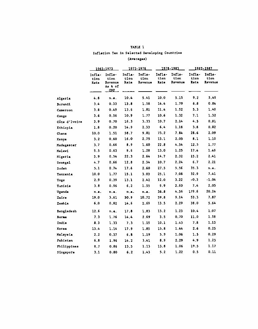
TABLE I

Inflation Tax in Selected Developing Countries

(Averages)

1963-1973 1973-1978 1978-1983 1983-1987

Infla- Infla- Infla- Infla- Infla- Infla- Infla- Infla-tion tion tion tion tion tion tion tion

Rate Revenue Rate Revenue Rate Revenue Rate RevenueAs % of

_______ GNP _______ ________ _______ ________ _______ ________

Algeria 4.8 n.a. 10.4 5.41 10.0 5.15 9.2 5.49

Burndi 3.4 0.33 13.8 1.58 14.4 1.79 6.8 0.84

Caaeroon 3.8 0.49 13.6 1.81 11.4 1.52 5.3 1.40

Congo 3.6 0.56 10.9 1.77 10.6 1.32 7.1 1.32

Cte d'Ivoire 3.9 0.70 16.3 3.33 10.7 2.14 4.5 0.81

Ethiopia 1.8 0.20 14.9 2.33 6.4 1.18 3.8 0.82

Ghana 10.0 1.51 58.7 9.81 73.2 7.84 28.6 2.09

Kenya 3.2 0.60 16.0 2.75 13.1 2.05 8.1 1.10

Madagascar 3.7 0.66 8.9 1.60 22.8 4.54 12.5 1.77

Malavi 5.5 0.63 9.6 1.28 13.0 1.25 17.4 1.49

Nigeria 5.9 0.54 22.3 2.64 14.7 2.32 15.2 2.41

Senegal 4.7 0.66 12.8 2.34 10.7 2.24 6.7 2.21

Sudan 5.1 0.74 17.6 2.60 27.5 5.56 35.3 na.

Tanzania 10.0 1.77 15.1 3.03 25.1 7.08 32.9 7.41

Togo 2.9 0.39 13.1 2.42 12.0 3.22 -0.3 -1.04

Tunisia 3.8 0.96 6.2 1.55 9.9 2.60 7.4 2.05

Uganda ma. n.e. n.e. n.e. 36.8 4.56 179.6 20.24

Zaire 19.0 3.61 50.9 10.72 59.8 9.14 53.3 7.87

Zambia 6.0 0.82 14.6 2.69 13.5 2.29 38.0 5.64

Bangladesh 12.6 na. 17.8 1.83 13.2 1.23 10.4 1.07

Burma 7.3 1.76 14.4 2.69 3.5 0.70 11.0 1.58

India 8.3 1.33 7.3 1.15 10.1 1.43 7.8 1.13

Korea 13.4 1.14 17.9 1.85 15.8 1.44 2.6 0.25

Malaysia 2.2 0.37 6.8 1.19 5.9 1.06 1.5 0.29

Pakistan 6.8 1.96 14.2 3.41 8.9 2.29 4.9 1.23

Philippines 8.7 0.86 13.5 1.13 13.8 1.06 19.5 1.17

Singapore 3.1 0.80 6.2 1.43 5.2 1.22 0.5 0.11

Table 1 (cont.

1963-1973 1973-1978 1978-1983 1983-1987In.fla- Infla- Infla- Infla- Infla- Infla- Infla- Infla-tion tion tion tion tion tion tion tionRat. Revenue Rats Revenue Rats Revenue Rate Revenue

As % of__ CNP

Sri Lanka 4.3 0.68 6.7 0.83 15.9 1.89 8.5 0.91

Greece 3.9 0.69 15.7 2.82 21.9 3.64 19.3 2.81

Spain 7.4 2.13 18.4 5.34 14.5 3.62 8.5 2.12

Portugal 6.2 3.36 23.3 11.08 21.6 7.32 17.4 6.36

Turkey 7.7 1.63 24.9 5.03 53.8 7.73 41.7 4.61

Yugoslavia 15.1 3.53 16.9 4.55 32.7 7.54 84.4 9.38

South Africa 4.5 0.75 11.5 1.63 13.8 1.92 15.7 2.73

Argentina 30.3 n.a. 200.1 25.03 174.7 12.04 380.1 22.00

Bolivia 8.4 0.85 18.7 1.71 99.6 8.67 524.1 105.68

Brazil 34.5 5.20 36.2 4.42 96.2 6.66 199.7 8.24

Chile 65.7 24.95 244.7 13.06 25.1 1.45 22.5 1.27

Colombia 11.5 1.71 23.7 3.12 24.6 2.94 20.6 1.97

Coats Rica 3.8 0.62 12.2 1.85 37.4 5.93 13.9 2.19

Dominican Rep. 3.4 0.35 10.4 1.04 9.2 0.82 24.7 2.33

Ecuador 6.1 0.91 14.8 2.34 20.9 3.28 27.9 3.64

El Salvador 1.6 0.19 13.6 1.82 14.4 2.29 22.7 3.25

Honduras 2.9 0.29 8.1 0.92 11.4 1.32 3.7 0.52

Jamaica 5.8 0.62 20.1 2.51 17.5 2.46 18.8 2.95

Mexico 4.6 0.53 20.2 2.05 46.6 3.93 85.3 4.36

Nicaragua 27.1 3.38 7.9 0.91 32.6 6.14 462.1 8.61

Paraguay 3.8 0.34 11.3 1.02 16.9 1.62 24.8 1.97

Peru 9.9 1.32 33.9 5.54 75.4 7.35 109.4 8.04

Uruguay 62.2 7.82 62.4 5.68 46.5 3.81 66.9 4.42

Venezuela 2.4 0.31 8.2 1.44 13.2 2.52 15.8 2.83

Sample StandardDeviation 13.1 3.7 42.5 4.1 30.5 2.7 109.9 15.1

Inflation R.ate — line 64x (CPI)Inflation Revenue — (line 64x) x (line 34) + (line 99b)

Inflation Rate times the ratio Money/CDP

Source: IFS. Tapes

TABLE 2

Augaented Dickey-Fuller Unit Root Tests for

Inflation and Taxes: Selected Developing Nations

Country Inflation Taxes

Brazil -0.172 -0.714 -2.278 -1.521

Burma -2.437 -2.721 -0.709 -0.069

Burundi -1.415 -0.634 -1.178 -1.876

Ecuador -0.008 -2.732 -0.216 -1.811

El Salvador -0.693 -2.419 -2.169 -2.197

Ethiopia -1.422 -1.128 -0.808 -2.188

Ghana -1.580 -1.850 -0.868 -1.646

Greece -0.064 -2.265 -1.000 -1.189

Honduras -1.434 -1.373 -0.320 -2.768

India -3.216* -4.150* -2.640 -2.748

Jamaica -0.818 -1.390 -0.520 -1.729

Kenya -1.731 -1.118 -1.179 -2.969

Malaysia -1.903 -2.040 -0.004 -1.719

Nigeria -1.260 -1.753 -1.689 -0.281

Pakistan -2.138 -2.369 -1.213 -2.075

Philippines -1.233 -2.608 -2.436 -2.601

Singapore -1.972 -1.677 2.019 1.005

South Africa -0.001 -2.707 0.003 -2.761

Yugoslavia -2.772 -1.901 -0.835 -2.452

Zambia -0.534 -1.593 -0.065 -3.255

QI: T tests the hypothesis of unit root without a time trend, while Tt

includes a time trend. The critical values of these tests at 95%

confidence for 25 observations are T — -3.0 and Tt — -3.6.

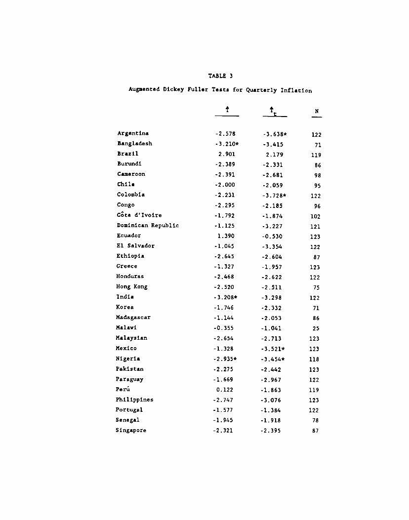
TABLE 3

Augnented Dickey Fuller Tests for Quarterly Inflation

t N

Argentina -2.578 .3.638* 122

Bangladesh .3.210* -3.415 71

Brazil 2.901 2.179 119

Bunmdi -2.389 -2.331 86

Cameroon -2.391 -2.681 98

Chile -2.000 -2.059 95

Colombia -2.231 .3.728* 122

Congo -2.295 -2.185 96

Cte d'Ivoire -1.792 -1.874 102

Dominican Republic -1.125 -3.227 121

Ecuador 1.390 -0.530 123

El Salvador -1.045 -3.354 122

Ethiopia -2.645 -2.604 87

Greece -1.327 -1.957 123

Honduras -2.468 -2.622 122

Hong Kong -2.520 -2.511 75

India .3.208* -3.298 122

Korea -1.746 -2.332 71

Madagascar -1.144 -2.053 86

Malawi -0.355 -1.041 25

Malaysian -2.654 -2.713 123

Mexico -1.328 -3.521* 123

Nigeria .2.935* 3454* 118

Pakistan -2.275 -2.442 123

Paraguay -1.669 -2.967 122

Peri 0.122 -1.863 119

Philippines -2.747 -3.076 123

Portugal -1.577 -1.384 122

Senegal -1.945 -1.918 78

Singapore -2.321 -2.395 87

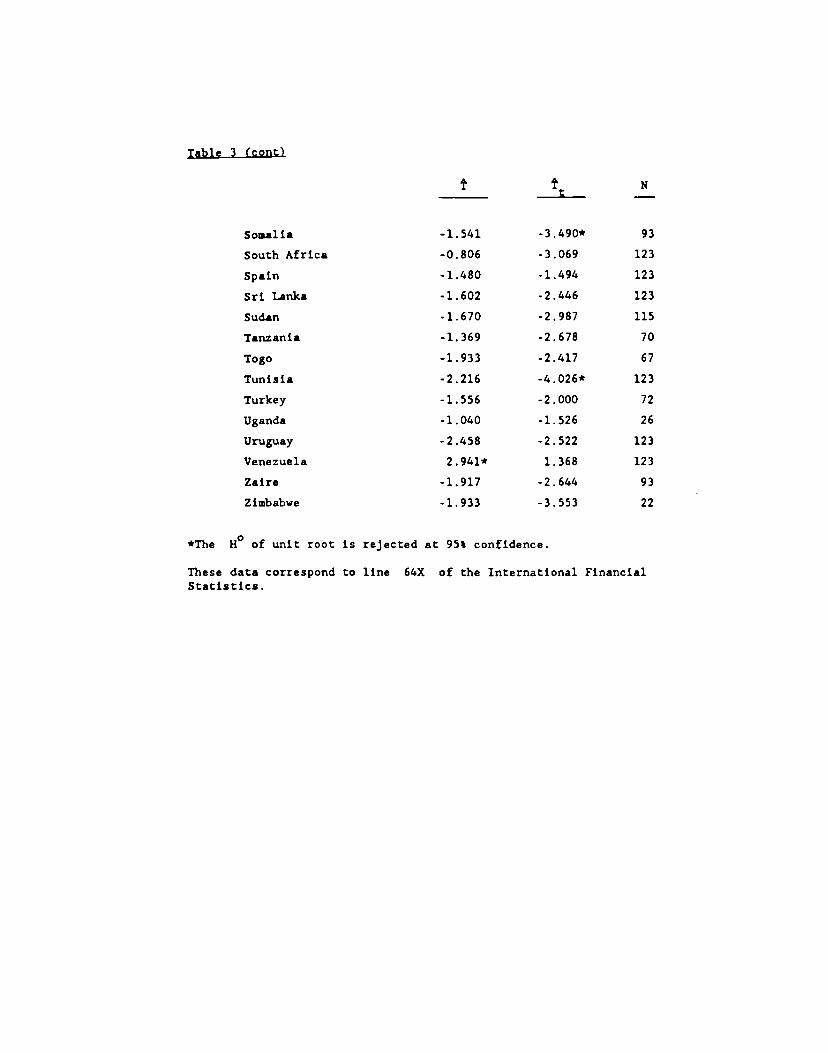
Table 3 (contl

N

Somalia -1.541 3•49Q* 93

South Africa -0.806 -3.069 123

Spain -1.480 -1.494 123

Sri Lanka -1.602 -2.446 123

Sudan -1.670 -2.987 115

Tanzania -1.369 -2.678 70

Togo -1.933 -2.417 67

Tunisia -2.216 4.026* 123

Turkey -1.556 -2.000 72

Uganda -1.040 -1.526 26

Uruguay -2.458 -2.522 123

Venezuela 2.941* 1.368 123

Zaire -1.917 .2.644 93

Zimbabwe -1.933 -3.553 22

*The H° of unit root is rejected at 95% confidence.

These data correspond to line 64X of the International FinancialStatistics.

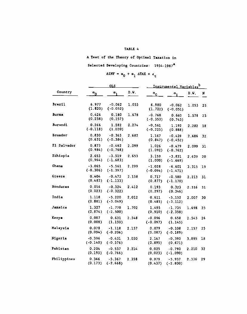
TABLE 4

A Test of the Theory of Optimal Taxation in

Selected Developing Countries: l954-l987

AINF—a0+a1TAX+ e

OLS Instrwnental Vprjpb1es'

Country a0 D.W. D.W. N

Brazil 6.977 -0.062 1.035 6.980 -0.062 1.053 25(1.820) (-0.052) (1.722) (-0.051)

Burma 0.426 0.180 1.678 -0.768 0.660 1.578 23(0.238) (0.257) (-0.353) (0.743)

Burundi 0.266 1.282 2.274 -0.561 1.192 2.282 18(-0.118) (1.020) (-0.225) (0.888)

Ecuador 0.830 -0.365 2.682 1.167 -0.439 2.686 32(0.631) (-0.384) (0.847) (-0.452)

El Salvador 0.873 -0.462 2.099 1.026 -0.479 2.099 31(0.984) (-0.768) (1.092) (-0.762)

Ethiopia 2.653 -3.519 2.653 3.159 -3.831 2.639 20(0.964) (-1.683) (1.000) (-1.669)

Ghana -3.065 -5.561 2.299 -1.028 -6.601 3.315 19(-0.306) (-1.397) (-0.094) (-1.471)

Greece 0.404 -0.472 2.158 0.717 -0.580 2.213 31(0.482) (-1.133) (0.877) (-1.170)

Honduras 0.016 -0.324 2.412 0.193 0.323 2.316 31(0.023) (-0.322) (0.297) (0.346)

India 1.118 -5.220 2.012 0.611 -5.152 2.007 30(0.881) (-3.049) (0.485) (-3.112)

Jamaica 1.327 -1.770 1.702 1.495 -1.735 1.698 25(0.874) (-2.500) (0.910) (-2.358)

Kenya 0.007 0.631 2.548 -0.096 0.658 2.543 26(0.008) (1.150) (-0.097) (1.145)

Malaysia 0.078 -1.118 2.157 0.079 -0.108 2.157 25(0.094) (-0.206) (0.087) (-0.189)

Nigeria -0.396 -0.431 3.030 2.147 -0.390 3.095 18(-0.140) (-0.576) (0.895) (0.671)

Pakistan 0.204 -0.537 2.214 0.025 -0.790 2.210 32(0.195) (-0.766) (0.023) (-1.090)

Philippines 0.366 -5.367 2.358 0.979 -5.937 2.336 29(0.173) (-2.668) (0.437) (-2.800)

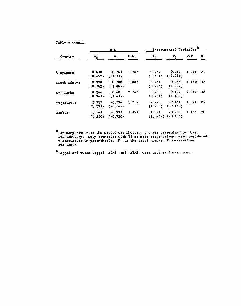
Table 4 (cont).

OLS Instrumental Vprjpblesb

Country 0p a1D.V. a _______

D.V. N

Singapore 0.638 -0.763 1.747 0.782 -0.782 1.746 21(0.452) (-1.335) (0.501) (-1.288)

South Africa 0.228 0.780 1.887 0.251 0.755 1.880 32

(0.762) (1.865) (0.798) (1.772)

Sri Lanka 0.246 0.601 2.342 0.289 0.610 2.340 32(0.267) (1.435) (0.294) (1.400)

Yugoslavia 2.717 -0.394 1.316 2.779 -0.456 1.304 25(1.397) (-0.665) (1.293) (-0.653)

Zambia 1.547 -0.232 1.897 1.394 -0.233 1.899 20(1.250) (-0.750) (1.0207) (-0.698)

AF0r many countries the period was shorter, and was determined by dataavailability. Only countries with 18 or more observations were considered.t-statistics in parenthesis. N is the total number of observationsavailable.

bLagged and twice lagged MNF and TAX were used as instruments.

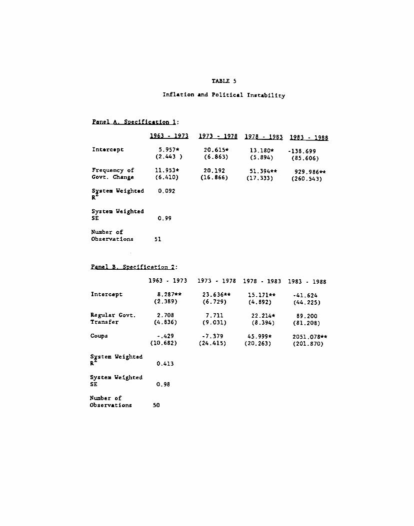
TABLE 5

Inflation end Political Instability

Panel A. Steciflcetion 1:

1963 1973 1973 - 1978 1978 1983 1983 - 1988

Intercept 5957* 20.615* 13.180* -138.699(2.443 ) (6.863) (5.894) (85.606)

Frequency of 11.953* 20.192 51.394** 929.986**Govt. Change (6.410) (16.866) (17.333) (260.543)

Sptem Weighted 0.092R

System WeightedSE 0.99

Number ofObservations 51

Panel B. St,ecificatjon 2:

1963 - 1973 1973 - 1978 1978 1983 1983 - 1988

Intercept 8.287** 23.636** 15.171** -41.624(2.389) (6.729) (4.892) (44.225)

Regular Govt. 2.708 7.711 22.214* 89.200Transfer (4.836) (9.031) (8.394) (81.208)

Coups -.429 -7.379 45999* 2051.078**(10.682) (24.415) (20.263) (201.870)

Sptem WeightedR 0.413

System WeightedSE 0.98

Number ofObservations 50

Table 5 (cont).

The dependent variable is the average rate of inflation over the relevanttime interval.

Standard errors in parentheses.

Method of estimation: the samples corresponding to the 4 subperiods werepooled and then seemingly unrelated regressions were used.

* : significant at the 5% level.** : significant at the 1% level.

TABLE 6

Trade Taxes and Political Instability

(Ordinary Least Squares)

(1) (2) (3)

Intercept O.4616** 0.0834 0.0927(0.0001) (0.0654) (0.0604)

Agriculture 0.0065** 0.0059**(0.0014) (0.0013)

Mining and Manufacturing .0.0071** -

(0.0012)

Foreign Trade 0.0061 0.0401 0.0329(0.0310) (0.0357) (0.0330)

CD? per Capita 0.69E-5 -0.22E-5 -0.42E-5(O.50E-5) (O.47E-5) (O.43E-5)

Urbanization .0.0025* •0.0003** -0.0002(0.0006) (0.0008) (0.0007)

Industrialized -0.1619** -0.0917 -0.0573(0.0379) (0.0522) (0.0394)

Latin Aserica - -0.0003(0.0417) -

Political Instability 0.1113 0.0317

(0.0904) (0.0980)

Regular Government - - -0.0277Transfers (0.0385)

Coups Frequency - - 0.1544(0.1267)

ft2 0.712 0.675 0.681

MSE 0.085 0.091 0.089

N 61 61 61

Means significant at 5% level;Means significant coefficient at 1%level.

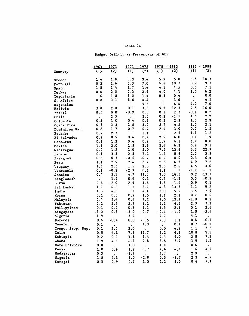
TABLE 7A

Budget Deficit as Percentage of CDP

1963 - 1973 1973 - 1978 1978 - 1983 1983 - 1988

Country (1) (2) (1) (2) (1) (2) (1) (2)

Greece 1.4 1.8 3.3 3.4 5.9 5.8 6.5 10.3

Portugal .0.2 1.6 5.3 7.0 4.6 10.7 0.7 9.7

Spain 1.8 1.4 1.7 1.4 4.1 4.5 0.5 7.1Turkey 0.4 2.5 2.3 2.9 4.0 4.1 1.0 6.2Yugoslavia 1.0 1.0 1.5 1.4 0.3 0.4 . 0.0S. Africa 0.8 3.1 1.0 4.4 . 3.6 . 4.5

Argentina . . . 5.3 . 6.4 7.0 7.0

Bolivia 3.8 2.8 0.1 3.8 5.5 12.3 2.5 16.0

Brazil 0.5 0.0 -0.9 0.3 0.1 2.3 -0.1 8.2

Chile . 2.5 . 2.0 0.2 -1.5 1.5 2.2

Colombia 0.5 1.0 0.4 0.2 0.2 2.3 1.5 2.8

Costa Rica 0.3 3.3 1.5 3.0 2.7 4.2 1.0 2.1

Dominican Rep. 0.8 1.7 0.7 0.4 2.4 3.0 0.7 1.5

Ecuador 0.7 2.7 . 1.1 . 2.5 1.1 1.2

El Salvador 0.2 0.5 0.4 0.2 2.9 4.0 0.1 1.9

}onduras 0.2 1.3 0.4 0.9 1.9 4.1 1.2 8.0

Mexico 1.1 2.0 1.8 3.9 3.4 6.3 5.9 9.1Nicaragua 0.0 1.2 1.0 5.0 7.5 13.6 3.3 22.9Panama 0.1 3.3 2.5 7.4 1.2 8.6 2.2 5.2

Paraguay 0.3 0.3 -0.6 -0.2 0.2 0.0 0.4 0.4Peru 1.1 2.9 2.4 5.2 2.3 4.3 4.0 7.2

Uruguay 1.6 2.3 1.5 2.3 2.5 2.6 4.5 3.0

Venezuela -0.1 -0.2 -2.9 0.6 1.1 1.6 -1.2 -1.2

Jamaica 0.4 3.1 4.7 11.3 8.0 16.3 0.2 13.7Bangladesh . 1.9 0.9 0.3 0.7 -1.2 0.3 -0.8

Burma 2.8 -2.0 2.9 1.8 -3.3 -1.2 -0.9 0.1Sri Lanka 1.1 6.6 1.2 6.7 4.3 13.3 1.1 9.2India 1.3 4.3 1.3 4.1 3.0 5.9 3.5 7.9

Korea 0.1 0.8 0.9 1.5 1.1 2.1 0.2 0.6Malaysia 0.4 5.4 0.6 7.2 1.0 13.1 -1.0 8.2Pakistan 2.2 5.7 2.7 8.1 3.2 6.6 2.3 7.2Philippines 0.4 0.9 0.3 1.1 1.3 2.1 0.2 2.6Singapore -3.0 0.3 -3.0 -0.7 -0.4 -1.9 1.0 -2.4Algeria 1.9 . 3.2 . 2.7 . 5.1 .

Burundi 0.6 -0.4 0.0 -0.5 2.3 1.1 0.8 -0.1Cameroon 0.1 . . 1.3 . 0.1 0.7 -0.2Congo, Peop. Rep. 0.1 2.2 2.0 . 0.0 4.8 1.1 3.3

Zaire 0.5 4.1 7.3 13.7 5.2 6.8 10.8 2.8Ethiopia 0.2 0.9 1.8 3.4 2.4 6.0 3.0 9.2Ghana 1.9 4.8 6.1 7.8 3.5 5.7 3.9 1.2

Cote D'Ivoire 0.0 . 1.0 . 1.8 . 0.0 .

Kenya 1.0 3.8 1.2 3.7 2.4 4.1 1.6 4.2

Madagascar 0.3 . -1.8 . 6.7 . 2.9 .

Nigeria 1.5 2.1 1.0 -2.8 3.3 -8.7 2.3 4.7

Senegal 0.5 0.9 0.7 1.5 2.2 2.5 0.6 7.1

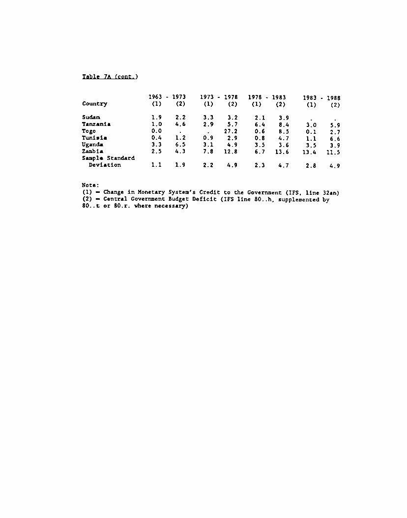
Table 7A (cont.)

Country1963 - 1973(1) (2)

1973 - 1978(1) (2)

1978 - 1983(1) (2)

1983 - 1988(1) (2)

(1) — Change in Monetary System's Credit to the Government (IFS, line 32an)(2) — Central Government Budget Deficit (IFS line 80. .h, supplemented by80. . t or 80.r. where necessary)

Sudan 1.9 2.2 3.3 3.2 2.1 3.9Tanzania 1.0 4.6 2.9 5.7 6.4 8.4 3.0 5.9Togo 0.0 . . 27.2 0.6 8.5 0.1 2.7Tunisia 0.4 1.2 0.9 2.9 0.8 4.7 1.1 6.6Uganda 3.3 6.5 3.1 4.9 3.5 3.6 3.5 3.9Zambia 2.5 4.3 7.8 12.8 6.7 13.6 13.4 11.5Sample Standard

Deviation 1.1 1.9 2.2 4.9 2.3 4.7 2.8 4.9

Note:

TABLE 7B

Correlation between Two Measures of Budget Deficit

Periods Correlation Coefficients

1963-73 .34

1973-78 .79

1978-83 .64

1983-88 .30

Pearson Correlation coefficients between columns (1) and (2) in Table 7A.

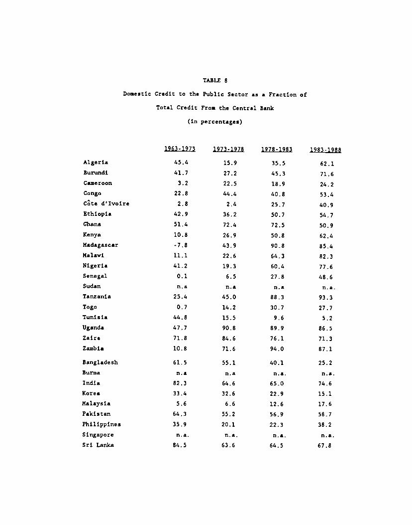
TABLE 8

Doiieatic Credit to the Public Sector as a Fraction of

Total Credit From the Central Bank

(in percentages)

1963-1973 1973-1978 1978-1983 1983-1988

Algeria 45.4 15.9 35.5 62.1

Burundi 41.7 27.2 45.3 71.6

Cameroon 3.2 22.5 18.9 24.2

Congo 22.8 44.4 40.8 53.4

Cate d'Ivoire 2.8 2.4 25.7 40.9

Ethiopia 42.9 36.2 50.7 54.7

Chana 51.4 72.4 72.5 50.9

Kenya 10.8 26.9 50.8 62.4

Madagascar -7.8 43.9 90.8 85.4

Malavi 11.1 22.6 64.3 82.3

Nigeria 41.2 19.3 60.4 77.6

Senegal 0.1 6.5 27.8 48.6

Sudan n.a n.a n.a n.e.

Tanzania 25.4 45.0 88.3 93.3

Togo 0.7 14.2 30.7 27.7

Tunisia 44.8 15.5 9.6 5.2

Uganda 47.7 90.8 89.9 86.5

Zaire 71.8 84.6 76.1 71.3

Zambia 10.8 71.6 94.0 87.1

Bangladesh 61.5 55.1 40.1 25.2

Burma n.a n.e n.a. n.a.

India 82.3 64.6 65.0 74.6

Korea 33.4 32.6 22.9 15.1

Malaysia 5.6 6.6 12.6 17.6

Pakistan 64.3 55.2 56.9 58.7

Philippines 35.9 20.1 22.3 38.2

Singapore n.e. n.a. n.a. n.e.

Sri Lanka 84.5 63.6 64.5 67.8

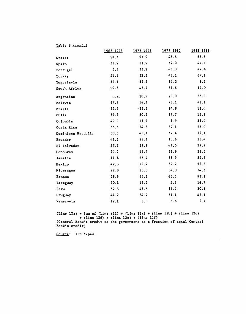
Table 8 (cont.

1963-1973 1973-1978 1978-1983 1983-1988

Greece 28.5 27.9 48.6 56.8

Spain 33.2 31.9 52.0 47.6

Portugal 5.6 33.2 46.3 47.4

Turkey 51.2 32.1 48.1 67.1

Yugoslavia 32.1 35.3 17.3 6.3

South Africa 29.8 45.7 31.6 12.0

Argentina n.e. 20.9 29.0 35.9

Bolivia 87.9 56.1 78.1 41.1

Brazil 32.9 -36.2 24.9 12.0

Chile 89.3 80.1 37.7 15.8

Colombia 42.9 13.9 6.9 33.4

Costa Rica 35.5 34.8 37.1 25.0

Dominican Republic 50.6 43.1 37.4 37.1

Ecuador 48.2 28.1 13.6 38.4

El Salvador 27.9 29.9 47.5 39.9

Honduras 24.2 18.7 31.9 38.5

Jamaica 11.6 65.4 88.5 82.3

Mexico 42.3 79.2 82.2 56.3

Nicaragua 22.8 25.3 54.0 74.3

Panama 59.8 63.1 65.5 83.1

Paraguay 50.1 13.2 5.3 16.7

Peru 52.3 45.5 35.2 30.8

Uruguay 44.2 34.2 31.1 46.1

Venezuela 12.1 3.3 8.6 6.7

(Line 12a) + Sum of (line (11) + (line l2a) + (line 12b) + (line l2c)+ (line 12d) + (line l2e) + (line 12f)

(Central Bank's credit to the government as a fraction of total CentralBank's credit)

Source: IFS tapes.

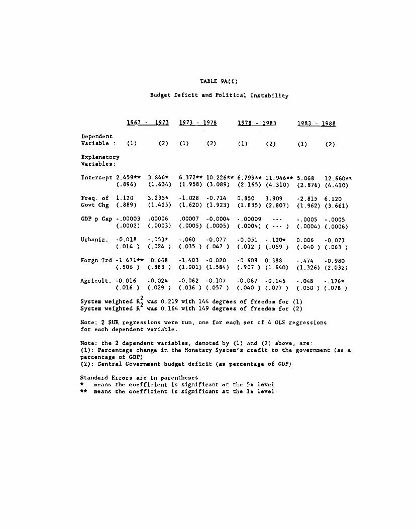
TABLE 9A(i)

Budget Deficit and Political Instability

1963 - 1973 1973 - 1978 1978 - 1983 1983 - 1988

DependentVariable : (1) (2) (1) (2) (1) (2) (1) (2)

ExplanatoryVariables:

Intercept 2.459** 3.846* 6.372** 10.226** 6.799** ll.946** 5.068 l2.660**(.896) (1.634) (1.958) (3.089) (2.165) (4.310) (2.876) (4.410)

Freq. of 1.120 3.235* -1.028 -0.714 0.850 3.909 -2.815 6.120Govt Chg (.889) (1.425) (1.620) (1.923) (1.835) (2.807) (1.962) (3.661)

GDP p Cap - .00003 .00006 .00007 -0.0004 -.00009 •- - - .0005 - .0005(.0002) (.0003) (.0005) (.0005) (.0004) ( --- ) (.0004) (.0006)

Urbaniz. -0.018 - .053* - .060 -0.077 -0.051 - .120* 0.006 -0.071(.014 ) (.024 ) (.035 ) (.047 ) (.032 ) (.059 ) (.040 ) (.063 )

Forgn Trd 1.67l** 0.668 -1.403 -0.020 -0.608 0.388 - .474 -0.980(.506 ) (.883 ) (1.001) (1.584) (.907 ) (1.640) (1.326) (2.032)

Agricult. -0.016 -0.024 -0.062 -0.107 -0.067 -0.145 - .048 - .176*(.016 ) (.029 ) (.036 ) (.057 ) (.040 ) (.077 ) (.050 ) (.078 )

System weighted R was 0.219 with 144 degrees of freedom for (1)System weighted R was 0.164 with 149 degrees of freedom for (2)

Note: 2 SUR regressions were run, one for each set of 4 OLS regressionsfor each dependent variable.

Note: the 2 dependent variables, denoted by (1) and (2) above, are:(1): Percentage change in the Monetary System's credit to the government (as apercentage of GDP)(2): Central Government budget deficit (as percentage of CDP)

Standard Errors are in parentheses* means the coefficient is significant at the 5% level** means the coefficient is significant at the 1% level

TABLE 9A(ii)


1963 - 1973 1973 - 1978 1978 - 1983 1983 - 1988



Intercept 0.563 l.714** l.689** 3.839** 2.610** 3.769** 2.879** 3.83l**(.308) (.463 ) (.448 ) (.635 ) (.584 ) (1.033) (.667 ) (1.191)

Freq. of 1.052 2.296 -0.136 -1.105 0.985 3.814 -2.373 5.823Govt Chg (.961) (1.302) (1.270) (1.507) (1.729) (2.623) (1.852) (3.408)

System weighted was 0.994 with 160 degrees of freedom for (1)System weighted R was 0.984 with 168 degrees of freedom for (2)


Note: the 2 dependent variables, denoted by (1) and (2) above, are:(1): Percentage change in the Monetary System's credit to the government (as apercentage of GD?)(2): Central Government budget deficit (as percentage of GDP)


TABLE 9B(i)


1963 - 1973 1973 - 1978 1978 - 1983 1983 - 1988



Intercept 2.497** 3.961* 5.120* 9.574** 7.494** 11.542* 5.135 13.667**(.824 ) (1.707) (1.962) (3.155) (2.187) (4.377) (3.133) (4.952)

Reg Govt. - .478 0.139 1.063 0.652 -0.831 1.470 -1.562 1.493Transfrs (.500 ) (.948 ) (.860 ) (1.075) (1.202) (1.753) (1.345) (2.265)

Coups 4.146** 4.623 -2.199 -0.024 4.237 4.872 0.860 7.719(1.355) (2.498) (1.502) (2.098) (2.212) (3.223) (2.375) (4.398)

GDP p Cap .00006 .0001 - .0007 - .0008 .0002 - -- - .0004 - .0004(.0002) (.0004) (.0005) (.0006) (.0004) ( --- ) (.0005) (.0006)

Urbaniz. -0.021 -0.050 -0.013 -0.054 -0.066 -0.107 -0.002 - .063(.014 ) (.026 ) (.039 ) (.051 ) (.034 ) (.059 ) (.045 ) (.066 )

Forgn Trd 1.470** 0.903 -1.203 0.342 -0.252 0.493 -0.224 -1.342(.476 ) (.939 ) (.977 ) (1.595) (.911 ) (1.638) (1.355) (2.006)

Agricult. -0.016 -0.021 -0.048 -0.104 -0.081 -0.142 -0.054 0.l97*(.015 ) (.031 ) (.037 ) (.059 ) (0.041) (.080 ) (.054 ) (.085 )



Note: the 2 dependent variables, denoted by (1) and (2) above, are:(1): Percentage change in the Monetary System's credit to the government (as apercentage of GDP)(2): Central Government budget deficit (as percentage of CDP)


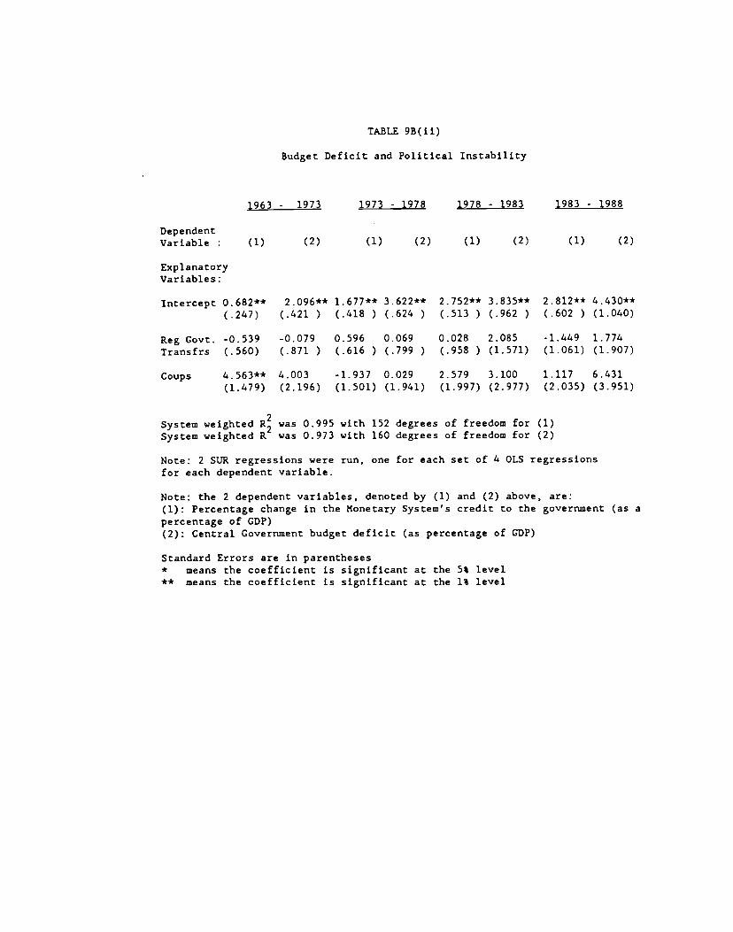
TABLE 9B(ii)


1963 - 1973 1973 - 1978 1978 - 1983 1983 - 1988



Intercept 0.682** 2.096** l.677** 3.622** 2.752** 3..835** 2.812** 4.430**

(.247) (.421 ) (.418 ) (.624 ) (.513 ) (.962 ) (.602 ) (1.040)

Reg Govt. -0.539 -0.079 0.596 0.069 0.028 2.085 -1.449 1.774

Transfrs (.560) (.871 ) (.616 ) (.799 ) (.958 ) (1.571) (1.061) (1.907)

Coups 4.563** 4.003 -1.937 0.029 2.579 3.100 1.117 6.431

(1.479) (2.196) (1.501) (1.941) (1.997) (2.977) (2.035) (3.951)


Note: 2 SUR regressions were run, one for each Set of 4 OLS regressionsfor each dependent variable.

Note: the 2 dependent variables, denoted by (1) and (2) above, are:(1): Percentage change in the Monetary System's credit to the government (as apercentage of GDP)(2): Central Government budget deficit (as percentage of GDP)


TABLE 1OA


1963 - 1973 1973 - 1978 1978 - 1983 1983 - 1988

DependentVariable (1) (2) (1) (2) (1) (2) (1) (2)


Intercept 1.283** 2.761** 2.953** 4.991** 3.46l** 4.376* 3.168** 3759(.397) (.642 ) (.763 ) (1.218) (.851 ) (1.754) (1.112) (1.986)

Freq. of 1.330 2.875* 0.093 -1.012 1.415 4.447 -2.984 6.269Govt Cbg (.939) (1.271) (1.241) (1.555) (1.757) (2.699) (1.843) (3.561)

Urbaniz. .0.021* .Ø•Q3j* .0.033* -0.031 -0.024 -0.023 -0.003 -0.003(.008 ) (.013 ) (.016 ) (.025 ) (0.017) (.034 ) (0.021) (.033 )

System weighted R2 was 0.988 with 156 degrees of freedom for (1)System weighted R2 was 0.984 with 160 degrees of freedom for (2)

Note: 2 STiR regressions were run, one for each set of 4 OLS regressionsfor each dependent variable.

Note: the 2 dependent variables, denoted by (1) and (2) above, are:(1): Percentage change in the Moneatry System's credit to the government (as a

percentage of GDP)(2): Central Government budget deficit (as percentage of GDP)


TABLE lOB


1963 - 1973 1973 - 1978 1978 - 1983 1983 - 1988



Intercept l.315** 3.043** 2.945** 4.698** 3.457** 4.239* 2.813* 3.867*

(.356) (.653 ) (.750 ) (1.231) (.827 ) (1.721) (1.086) (1.881)

Reg Govt. -0.418 0.055 0.756 0.093 0.140 2.246 -1.641 1.830Transfers ( .547) (.863 ) (.593 ) (.819 ) (.980 ) (1.611) (1.051) (1.978)

Coups 4.492** 4.048 -2.089 0.034 2.512 3.375 1.256 6.881

(1.432) (2.169) (1.411) (1.975) (2.044) (3.035) (1.992) (4.106)

Urbaniz. 0.O17* 0.026* 0.033* -0.029 -0.019 -0.016 0.002 0.009

(.007 ) (.013 ) (.016 ) (.026 ) (.018 ) (.035 ) (.022 ) (.033 )

System weigited R2 was 0.993 with 148 degrees of freedom for (1)System weighted R2 was 0.976 with 152 degrees of freedom for (2)


Note: the 2 dependent variables, denoted by (1) and (2) above, are:(1): Percentage change in the Moneatry System's credit to the government (as a

percentage of CDP)(2): Central Government budget deficit (as percentage of CDP)


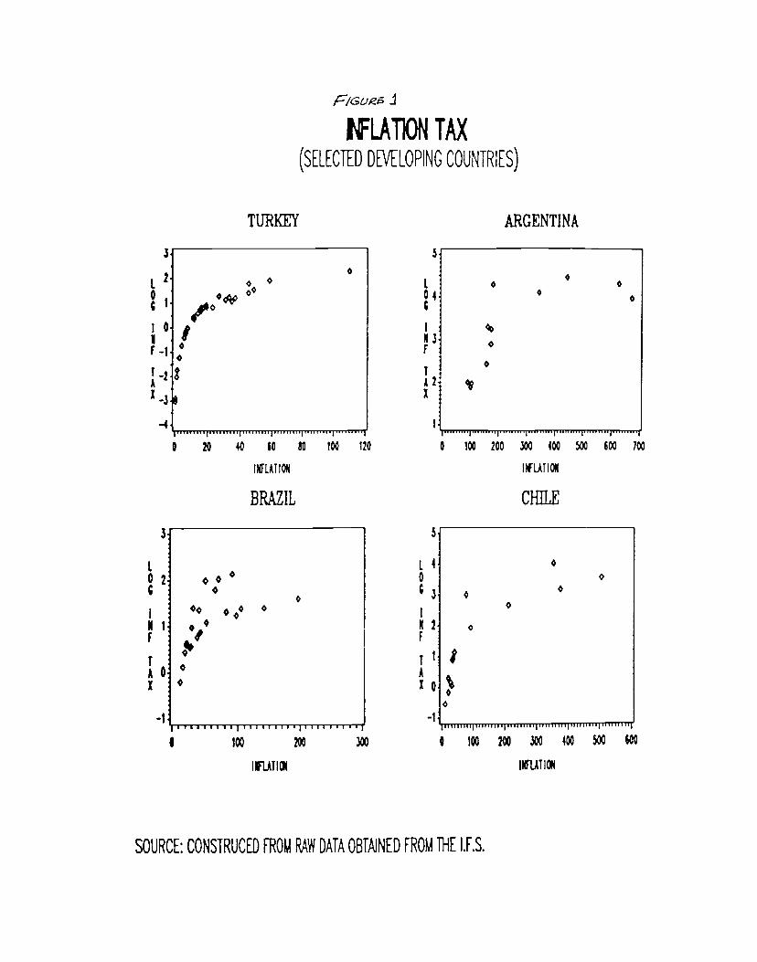
NLk11ON TAX

(SELECTED DEVELOPING COUNTRIES)

TURKEY ARGENTINA

3 5

i2o 04

C

101 II 'F-I:

1A A2

X_3X

-4 ___________ 1 ________I I•"'"'"I•'''•''''I'"'•••'l'•''''''•I'''''"''

0 20 40 60 80 100 120 0 100 200 300 400 500 600 700

tNFLATI0 fl(L'J100

BRAZIL CHILE

5

t 1402 0

I • 0I

*

Ni e K2F I FittA0 ° A

x_1

•

x_iI1IIII•1..'Il 5JuII'I1uIIII'0 0 IX 200 300 400 500 600

IuTI

SOURCE: CONSTRUCED FROU RAP1I DATA OBIAJNED FROA THE I.F.S.

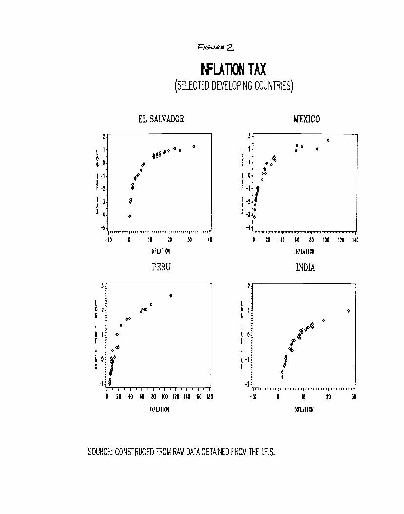
EL SALVADOR

-' atFLA11ON TAX

(SELECTED DEVELOPING COUNTRIES)

MEXICO

K

F

IAI

3

21

01l0N

F —

1A

x

I0C

F

IAI

—3

-4

SOURCE: CONSTRUCED RO RA1N DATA OBTAiNED FRO)1 THE LF.S.

10 20 40 60 80 100 120 140

JMFLATI

II4DIA

0*0

040

2

I0

1 —1

IF —2

I ..A

14

-

3

I02c

/

0

0

8

0

-10 0 10 20 30 40

INFLAI!

PERU

0

*00

4

V'I'I•I' J'I'I 111110 20 40 60 100 120 140 160 130

IXFLAT I

0

—l

2

0

—1

—2

0

0

IIrII,I,,Il,ryIII,,I,iyIIl,ITIl,,,l',,r-10 0 10 20 30

IXflA1Ic(

//cQ'.- 3

IFLAflON TAX

(SELECTED DEVtLOPINC COUNTRIES)

ETHIOPIA ZAIRE

2

01

0I 00 1 0

0 02CO C

I-I II NiF-2 F

I_i 0 1A A0I_4 I *

—5 ______________________________________ —1 ______________________________________

-10 0 10 20 30 -tO 10 30 50 70 110

INILAfl0 INILATI

COTE D IVOIRE TOGO

I 4 2

Os 4i 11 •O 0

00 0 $0cC

I-i $0I N

F2 •1 T_3A A

0 -4

11111111111111111111111111 111111 11111111 1111111 uulIulullIl lIjil 11111111 1111111

—10 0 tO 20 30 —10 0 IC 20 30

IU1I 91A1I

SOURCE: COSTRUCED ROA RAVi ATA OBTJNED FRO1 THE LF.S.

Documents

EtC - NBER