NBER WORKING PAPER SERIES

LIQUIDITY CONSTRAINTS AND HOUSING PRICES:THEORY AND EVIDENCE FROMTHE VA MORTGAGE PROGRAM

Jacob L. Vigdor

Working Paper 10611http://www.nber.org/papers/w10611

NATIONAL BUREAU OF ECONOMIC RESEARCH1050 Massachusetts Avenue

Cambridge, MA 02138June 2004

I thank Charles Clotfelter, William Collins, and seminar participants at the Triangle Applied MicroeconomicsConference, the University of Southern California and University of California, Berkeley for helpfulcomments on earlier drafts, and Carrie Ciaccia for excellent research assistance. The views expressed hereinare those of the author(s) and not necessarily those of the National Bureau of Economic Research.

©2004 by Jacob L. Vigdor. All rights reserved. Short sections of text, not to exceed two paragraphs, maybe quoted without explicit permission provided that full credit, including © notice, is given to the source.

Liquidity Constraints and Housing Prices: Theory and Evidence from the VA MortgageJacob L. VigdorNBER Working Paper No. 10611June 2004JEL No. D91, E21, G21, R21

ABSTRACT

This paper employs a simple intertemporal model to show that presence of liquidity constraints can

depress the price of a durable good below its net present rental value, regardless of the overall

supply elasticity. The existence of price effects implies that the relaxation of liquidity constraints

is not Pareto improving, and may in fact be regressive. Historical evidence, which exploits the fact

that a clearly identifiable group, war veterans, enjoyed the most favored access to mortgage credit

in the postwar era, supports the model. The results suggest that more recent mortgage market

innovations have served primarily to increase prices rather than home ownership rates, and that such

innovations have the potential to exacerbate socioeconomic disparities in ownership rates.

Jacob L. VigdorDuke UniversityBox 90245Durham, NC 27708and NBERjacob.vigdor@duke.edu

1

I. Introduction

In the United States, few policy goals inspire less political controversy than the promotion

of home ownership. Both Democratic and Republican administrations have cited increased home

ownership rates as an important priority, and have pointed towards recent increases in this rate as

an accomplishment. Since the Great Depression, government efforts to ease the path to home

ownership have focused on generating greater and more widespread access to credit markets. Such

efforts, described in detail in Section II below, concord with a view that liquidity constraints prevent

many households from engaging in socially preferred behavior.

In recent economic literature, the role of liquidity constraints in altering behavior is a matter

of some debate. A number of articles, both examining housing tenure (Duca and Rosenthal 1994;

Gyourko et al. 1999; Haurin et al. 1997; Linneman et al. 1997; Linneman and Wachter 1989;

Listokin et al. 2001; Rosenthal, 2002; Zorn 1989) and more general consumption patterns (Hayashi,

1985; Chah, Ramey, and Starr, 1995; Stepens, 2002) support the hypothesis that consumer behavior

changes in the presence of borrowing constraints. Borrowing constraints have frequently been

implicated as an explanation for empirical failures of the life-cycle and permanent income

hypotheses (see Deaton, 1992, for a thorough review). On the other hand, several prominent papers

have challenged the notion that liquidity constraints strongly influence behavior (Carneiro and

Heckman 2002; Cameron and Taber 2004; Hurst and Lusardi 2004). Households facing liquidity

constraints differ in many respects from unconstrained households, and it is these other differences

that may truly explain differences in observed behavior. If this is the case, then relaxing liquidity

constraints would have little or no impact on equilibrium consumption or investment patterns.

This paper focuses on a second reason why the relaxation of liquidity constraints may have

2

limited impact on behavior: because greater access to credit has the potential to raise the equilibrium

price of durable goods. Price effects may explain, for example, why numerous mortgage market

innovations over the past twenty years have had only a negligible impact on home ownership rates.

The possibility that liquidity constraints depress prices has been raised in previous theoretical

literature (Ranney 1981; Stein 1995; Ortalo-Magne and Rady 2002). Empirical studies, however,

often ignore the potential for price effects or assume that any such effects are negligible.

Does the relaxation of borrowing constraints lead to higher prices for assets and durable

goods? Is this effect large enough to be empirically relevant? Existing literature is largely mute on

these questions; this paper provides answers to each of them.

This study extends the existing theoretical literature on liquidity constraints and prices by

debunking the primary argument of those who claim that price effects are negligible: that highly

elastic long-run supply curves limit the potential for demand increases to translate into price

increases. A very simple intertemporal model, inspired by existing models of tenure choice in the

housing market (Artle and Varaiya, 1978; Brueckner, 1986; Henderson and Ioannides, 1983; Stein

1995), shows that borrowing constraint relaxation can make asset values rise relative to the present

discounted value of rents even when supply is perfectly elastic.

This study also presents an empirical analysis of liquidity constraints and prices that

examines both time-series evidence on the relation of housing values to rents and cross-sectional

variation generated by a large government program that selectively relaxed borrowing constraints

for a clearly identifiable subset of the population: the VA mortgage program. The evidence suggests

that mortgage market innovations contributed to a remarkable rise in housing values relative to rents

between 1940 and the present. In particular, the ratio of housing values to rents displays sensitivity

1 Economists may be skeptical of the importance of home ownership as an indicator of well-being, relativeto measures such as household income or consumption. Interest in home ownership can be justified on the groundsthat consumers are myopic and need to employ commitment devices in order to accumulate assets (Laibson 1997).There is also evidence that housing tenure decisions have nonmarket implications for child and family development(Boehm and Schlottmann, 1997; Green and White 1997) and citizenship (DiPasquale and Glaeser 1997; see Rohe etal. 2002 for a literature review). Finally, public economists take interest in home ownership because of the incometax treatment of mortgage payments and other policy initiatives (Engelhardt, 1997; Follain et al. 1987; Poterba,1992; Poterba 1984; see Hendershott and White 2000 for a literature review). See Collins and Margo (2001) andMasnick (2001) for analysis of home ownership patterns in the U.S. across the twentieth century.

3

to the share of veterans in the market in the time period when the VA mortgage program had the

greatest impact on home ownership rates. Section II below provides basic information on the

evolution of housing prices in this era; following the theoretical discussion in section III, section IV

presents time-series evidence and section V analyzes the implications of the VA mortgage program.

The existence of price effects implies that the relaxation of borrowing constraints, though

welfare improving by Hicks-Kaldor criteria, is not Pareto improving. If easier credit creates winners

and losers, how might we most accurately characterize consumers who gain and those who suffer?

While section III discusses this question in theory, section VI presents empirical evidence to suggest

that households of low socioeconomic status benefit least from innovations in the credit market.

Given the billions of dollars spent on improving access to mortgage markets and otherwise

subsidizing home ownership in the United States, the distributional implications of promoting easy

access to credit should be widely noted.

II. Motivating evidence: housing prices, the mortgage market, and home ownership

The mid-twentieth century witnessed a profound change in both home ownership patterns

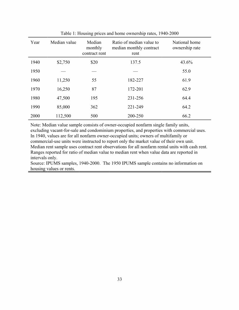
and the relationship between asset prices and rental rates in the housing market.1 As Table 1

indicates, the home ownership rate in the U.S. increased by nearly 50% between 1940 and 1960.

After 1960, ownership rates continued to increase, but at a markedly slower rate. Table 1 also shows

2 It is not possible to pinpoint the exact ratio after 1940 because housing value data are intervalled. Censusdata on housing prices and rents are not available prior to 1940.

3 The sample of owner-occupied units used to construct these statistics consists of nonfarm, non-condominium occupied single family units with no commercial uses, on lots of less than ten acres. In 1940, it is notpossible to distinguish multifamily units or units with commercial units, however respondents were instructed in thatyear to omit the value of units they did not occupy or commercial space when providing their estimate of marketvalue.

4 Figure 1 also shows that the price of owner-occupied housing fell relative to the price of other consumergoods during World War II. This may reflect the wartime rationing of goods other than owner-occupied housing.

4

that this marked increase in home ownership was accompanied by a substantial increase in the price

of the typical owner occupied housing unit, relative to the cost of the typical rental unit. In 1940,

the median owner-occupied housing unit was worth roughly 140 times median monthly rent. By

1960, this ratio had increased to at least 180.2 The ratio has remained at or above this general level

since, with some evidence of further increases in recent decades.3

This escalation, while impressive, may reflect changes in the physical characteristics of

owner- and renter-occupied units over time. A measure of constant-quality owner-occupied housing

prices can be obtained from the National Income and Product Accounts beginning in 1929. Figure

1 plots this price index, converted to a logarithmic scale, along with the corresponding price index

for all personal consumption expenditures. Both indices have been normalized to a value of zero

in 1947. This graph shows that over the postwar period, constant-quality housing values have

tracked overall price levels fairly closely, with two noteworthy exceptions. Housing prices

accelerated above inflation in the immediate postwar era and remained relatively higher than the

prices of other consumer goods until the mid-1970s.4 This pattern corroborates the acceleration of

owner-occupied housing values displayed in Table 1. In the late 1970s, housing prices tracked

general price levels quite closely, in spite of Beginning in 1982, housing prices began another period

5 Interestingly, these time series indicate that the period of rapid home price acceleration in the 1970s,analyzed by Mankiw and Weil (1989) and many subsequent researchers, can be viewed as a simple manifestation ofoverall price level increases or increases in housing unit quality over the same time period.

5

of acceleration.5 This acceleration has persisted to the present day.

These two periods of housing price escalation coincide with major relaxations in borrowing

constraints, as seen in the timeline of major mortgage market innovations presented in Table 2

(Jackson, 1985; Bruskin et al. 2000; Listokin et al. 2001; Martinez 2000). At the onset of the Great

Depression, when the time series graph in Figure 1 begins, families interested in purchasing a home

generally were expected to make a down payment of at least 30% of the home’s value. The loan

they received would not be fully amortized, requiring a balloon payment (or refinancing) after five

to ten years. During the depression, a large number of households defaulted on their mortgage

payments, leading to foreclosure in many cases. Over an eleven-year period beginning in 1933,

government innovations, including the creation of the Federal Housing Administration (FHA) and

Veterans’ Administration (VA) mortgage insurance programs, and the establishment of a secondary

market for mortgage debt, radically changed the nature of the mortgage market. By 1944, it was

possible for many households to receive a fully amortized, twenty to thirty-year mortgage with down

payments of 10% or less. The VA mortgage program was the most generous of those introduced

during this time period, since it enabled eligible veterans to purchase a home with no down payment

whatsoever and no mortgage insurance premium. As with the FHA program, the Federal

government insured lenders against default risk.

The impact of these innovations on home ownership rates and housing prices was somewhat

delayed by depression and war. Ownership rates reached a local minimum in the 1940 Census, and

Figure 1 shows that housing prices continued to sink relative to other consumer goods until the end

6

of World War II. The coincidence of rapidly increasing ownership rates and housing prices in the

postwar era suggests an important role for relaxed liquidity constraints.

The second period of escalating relative house prices, beginning around 1982, coincides with

further innovations in the mortgage market. Until the 1980s the secondary mortgage market, which

encouraged lending by pooling the risk that individual financial institutions assumed when extending

credit, was an avenue open only for loans that “conformed” to underwriting standards governing

borrower creditworthiness and property characteristics. A secondary market for “non-conforming”

loans, mortgages that entities such as the Federal National Mortgage Association (FNMA) refused

to securitize, grew rapidly through the 1980s and into the 1990s. The definition of “conforming”

loans was itself relaxed in response to Federal legislation in 1992. By 1994, lenders had initialized

programs that allowed qualified households to borrow more than the value of a home, effectively

creating a negative down payment that could be applied towards closing costs or received in cash.

These innovations enabled some previously ineligible households to purchase a home, and provided

many others with increased buying power given current wealth levels (Bruskin et al., 2000). As

Table 1 indicates, these new mortgage market innovations are not associated with any appreciable

change in home ownership rates. They do, however, coincide with the current period of relatively

high prices for owner-occupied housing, as shown in Figure 1.

Could factors other than credit market innovations explain these broad trends? Fluctuations

in real interest rates undoubtedly influence the ratio of housing prices to rents; however the trends

identified in this section are of too broad a period to be explained by cyclical variation. Changes

in the value of the tax subsidy for mortgage interest, which has been in place since 1913, might also

be expected to influence housing prices (Poterba, 1984). Note, however, that housing prices failed

6 In an appendix, Stein (1995) incorporates a rental market, but requires that renters pay an arbirtrarypremium relative to owner-occupied housing prices. This model can also generate such a premium as a result ofliquidity constraints, rather than by assumption.

7

to accelerate ahead of inflation during the “bracket creep” era of the late 1970s and 1980s. Prices

did accelerate, however, during the latter part of the 1980s, a time of broad declines in marginal tax

rates.

III. Tenure choice, liquidity constraints, and prices: a simple model

There have been several noteworthy theoretical studies of housing prices and more generally

of housing demand (Ranney, 1981; Poterba, 1984; Schwab 1982; Stein, 1995; Ortalo-Magne and

Rady 2002; see Smith et al. 1988 for a review of housing market models). Stein (1995), in

particular, uses a static model to show that borrowing constraints reduce housing prices. Stein’s

result can be attributed to the assumption of a fixed housing stock, and the fact that households must

pay for housing prior to consuming and earning income. Under different assumptions, particularly

if housing supply is close to perfectly elastic, this type of model produces radically different results.

The model presented here is an advancement over Stein’s model in several respects. It is a

two-period intertemporal model. There is no restriction on the price elasticity of housing supply.

Finally, there is a fully integrated rental market for housing as well as a market for owner-occupied

housing.6 The model shows that liquidity constraints can depress the price of owner-occupied

housing below the present value of rents, regardless of the local price elasticity of supply.

Agents i derive utility from two consumption goods, housing services Hi and a numeraire

commodity Xi. They are endowed with varying amounts of a single physical asset, Ai, which can

be interpreted as land. They are also endowed with varying amounts of effective labor, Li, which

8

they supply inelastically to firms. Competitive firms purchase labor and rent land in competitive

factor markets and transform them into the numeraire commodity. Any quantities of land not used

in the production process in a given period can be costlessly transformed into housing services. In

the first period, agents may buy, sell or rent land. Only consumers may purchase land, but either

consumers or firms may rent it. Agents’ net housing consumption in each period is Ai, less the net

amount sold and the net amount rented to other agents .

Using Xti to denote numeraire consumption in period t, assuming that utility is time-

separable, and that agents making decisions in the first period discount second-period utility by a

factor *, the consumer’s maximization problem can be stated as follows:

(1) ,

subject to the accounting identity

(2) .

Assuming that agents can store the numeraire commodity without risk or return between periods,

the maximization in equation (1) is undertaken subject to the lifetime budget constraint:

(3) ,

where w is the market wage, equal to the marginal product of effective labor, r equals the marginal

product of land in the production of the numeraire, and V is the endogenously determined price of

a unit of land.

Agents with asset holdings that are sufficiently small relative to their labor income will find

it desirable to borrow against their second period income. Such borrowing is governed by the

relation:

(4) .

7 Stiglitz and Weiss (1981) present a model justifying the existence of credit rationing in markets withimperfect information.

8 This model can thus endogenously generate premiums for rental housing, observationally equivalent todiscounts for owner-occupied housing, similar to those derived by Henderson and Ioannides (1983) and imposed byassumption in Stein (1995).

9 General equilibrium effects complicate this intuition somewhat. In practice, the equality required byequation (5) could be achieved either by a decrease in V or an increase in r. Under the assumption of diminishingmarginal product, higher r implies greater labor intensity and lower equilibrium wages. In general, lower wages willhave the effect of reducing liquidity constraints.

9

In words, excess of first-period consumption over total first-period income may not exceed :i.7 In

scenarios where borrowing is prohibited, :i=0. Less stringent regulations on borrowing involve

some greater value of :i.

With this setup, it is quite simple to show that per-unit housing values V fall below the

present value of rents, 2r, in the presence of liquidity constraints. Denoting the Lagrange multiplier

from the lifetime constraint (3) as 81 and the multiplier from the intertemporal constraint (4) as 82,

the first order conditions of the consumer’s problem yield the following relation between V and r:

(5) .

When the intertemporal constraint is nonbinding, this expression for V reduces to 2r, the present

value of rents. As liquidity constraints become more binding, increasing the shadow value of first-

period assets, this expression falls further below the present value of rents.8 Intuitively, liquidity

constraints drive consumers to sell land on the open market and consume housing by renting instead.

If the excess supply created by liquidity-constrained consumers wishing to sell land cannot be

absorbed by unconstrained consumers willing to buy, the equilibrium price must fall.9

The distributional implications of relaxing liquidity constraints are easily derived.

Consumers can be divided into two groups on the basis of their value of 82. Initially, less-

constrained households are net purchasers of housing, and realize the benefits of depressed prices

10 There is some empirical evidence to support the notion that credit access programs do not benefit thelong-term poor. Goodman and Nichols (1997) show evidence that the FHA mortgage program primarily benefitsyoung households – likely those with low asset holdings in relation to present and future income – rather than poorhouseholds.

10

either by increasing their housing consumption or renting additional units of land to finance

numeraire consumption. More-constrained households adopt the opposite strategy, selling to finance

additional numeraire consumption in the first period. Any general relaxation of liquidity constraints

naturally yields positive benefits to net sellers of housing and negative benefits to net purchasers.

In this model, less-constrained households will tend to be those with high asset holdings

relative to income, or equivalently low income in relation to asset holdings. It is thus difficult to

determine a priori whether the relaxation of liquidity constraints is progressive or regressive. If

households with low income also tend to have a low ratio of income-to-assets, then easier access to

credit can actually be a regressive policy.10

Another implication of this model, which will be of importance for the empirical tests below,

is that exogenous increases in the rental rate r should increase the discount applied to V. Intuitively,

since the net rental holdings of households are negative, a higher r increases per-period income

relative to net assets. Any increase in per-period income relative to asset holdings will increase

households’ desire to borrow to finance first-period consumption.

It is worth reiterating that this model’s result holds without any reference to the price

elasticity of supply for housing. In this model, the elasticity of housing supply depends on the

second derivative of firms’ production functions with respect to the physical asset. If the marginal

product of land is constant, then the elasticity of supply for housing is infinite: increases in demand

11 In this model, the housing supply elasticity can only be infinite up to a point – determined by the totalendowments of land in the economy. Also note that increased housing demand may have a feedback effect, sincereduced utilization of land may change the marginal product of labor in production, and hence wages.

12 Several empirical studies have concluded that the price elasticity of housing supply is considerably lessthan infinite (Capozza, Green and Hendershott 1996; Topel and Rosen 1988; Malpezzi and Mayo 1997).

13 Multifamily dwellings are excluded for all sample years except 1940. In 1940, owners of multifamilyunits were asked to estimate the value of their own unit only. It is not possible to determine which housing units arepart of multifamily structures in these data. Farms are also excluded from the analysis.

11

for housing translate entirely into changes in the quantity consumed.11 Even when the rental price

is constant, however, liquidity constraints can influence the purchase price of housing. Some

previous empirical studies of liquidity constraints and tenure choice dismiss the possibility of price

effects with arguments related to the supply elasticity of housing (see, for example, Monroe, 2001).12

The results presented in this section show that these arguments are insufficient to assuage concerns

that easier access to credit creates inflationary pressure in the housing market. The following

sections present empirical evidence documenting such effects.

IV. Time Series Evidence

As shown in Table 1, the ratio of median value to median rent has increased considerably

over the past sixty years. Table 3 presents the results of simple tests of the hypothesis that this

phenomenon reflects a gradual elimination of discounts for owner-occupied housing in high-rent

housing markets. As illustrated above, such a pattern would be expected if consumers in these

markets experienced a reduction in liquidity constraints.

These regressions make use of Integrated Public Use Microdata Sample (IPUMS) data

collected from a series of U.S. Census enumerations beginning in 1940. The unit of observation in

each specification is an owner-occupied housing unit.13 The dependent variable in each specification

14 Previous research has shown that owners tend to overestimate their property’s true market value, butestimation errors appear to be random (Goodman and Ittner, 1992). The 1940 value data are coded at the dollarlevel; the 1970 value data are intervalled.

15 Since the independent variable of interest is a sample statistic, each observation in the regression isweighted by the square root of the sample size used in calculating the statistic, in order to avoid heteroskedasticityproblems. Unweighted regressions yield similar results, though ln(rent) coefficients in both 1940 and 1970 aresmaller in absolute value, as should be expected when noisier observations are given greater weight in theregression.

16 Although the unit of observation in these regressions is an owner-occupied housing unit, the number ofindependent observations is effectively restricted to the number of MSAs in each year. For this reason, the Huber-White correction has been applied to the standard errors in these regressions.

17 In an infinite-horizon model without liquidity constraints, V = r/*. Taking logs, we find ln(V) = ln(r) -ln(*). The intercept of this regression can thus be interpreted as the negative value of the logarithm of the rate ofreturn used to compute housing values. The parameter estimates in Table 4 yield annual rates of return on the orderof 6.8 to 7.7 percent. One alternative interpretation of the slope coefficient in the 1940 regression is that the relevantrate of return on investments in high rent markets is higher.

18 In 1970, about 4% of owner-occupied housing units have topcoded value observations. This topcodingmost likely biases the rent coefficient downward; omission of topcoded observations from the sample results inlower coefficient estimates.

12

is the logarithm of the owner’s self-reported estimate of the unit’s market value.14 The independent

variable of primary interest is the logarithm of median rent in the housing market.15 In this and all

subsequent analyses, metropolitan statistical areas (MSAs) will serve as a proxy for a housing

market area.16

The estimation is hampered to some extent by the absence of data on housing structural

characteristics in the 1940 Census. For purposes of comparing results in 1940 and later years, Table

3 reports the results of 1970 specifications constrained to match the data limitations in 1940. Simple

univariate regressions of log housing values on log median rents, reported in the table’s first and

third columns, show a relationship that increases in magnitude between 1940 and 1970.17 The point

estimate in the first column suggests that metropolitan areas with higher rents in 1940 had less-than-

proportionately higher values. The 1970 point estimate suggests the reverse, that ratios of value to

rent were higher in high-rent markets.18 While suggestive, it should be noted that neither of these

19The 1940 IPUMS data lack information necessary to construct this data; omission of this variable fromthe 1970 regressions does not alter the results.

13

coefficients can be statistically distinguished from one, and they are not significantly different from

each other.

The ideal source of variation in median rents for this exercise would be exogenous

differences across markets in terms of local amenities or opportunity costs of supplying housing

units. The median rent data used here might confound this type of variation with that arising from

characteristics of a metropolitan area’s residents, most notably their income levels. To more

effectively isolate location-based variation in median rents, the remaining regressions in Table 3

control for a basic set of housing market characteristics, including householders’ median age, the

fraction of householders working in manufacturing industries, the fraction of householders with a

college education, and Census region effects. The 1970 regression also includes a measure of recent

housing supply growth, the fraction of all housing units built after 1960, to account for the

possibility that supply responses may have differentially closed gaps in rents and values across

housing markets.19

Controlling for housing market characteristics, the relationship between rents and values

across housing markets in 1940 weakens considerably. For every 1 percent increase in median rents,

predicted owner-occupied housing values increase by roughly 0.3 percent. A very different pattern

emerges in 1970: the effect of a 1 percent increase in median rent is statistically indistiguishable

from a 1 percent increase in values. The 1940 coefficient is significantly less than one and

significantly different from the 1970 coefficient. This pattern corresponds exactly to the model’s

predictions: in a liquidity-constrained world, housing values in high-rent areas are discounted; when

20 An alternative explanation for the patterns in Table 3 focuses on cyclical effects. Since housing valuesshould reflect the present discounted value of rents, rents should display more cyclical volatility than values. Inrecessions, the ratio of values to rents should be higher; in expansionary periods the ratio should be lower. According to the National Bureau of Economic Research, the 1940 Census was taken nearly two years into a sevenyear-long expansion, while the 1970 Census was taken in the midst of a nearly year-long recession. Note, however,that a universal reduction in the ratio of values to rents should alter the intercept term of these regressions, not thecoefficient on median rent. The median rent coefficient would change only if recessions differentially affect theratio of values to rents in high-rent markets.

21 Added structural characteristics include categorical variables for number of rooms, year structure built,presence of basement, number of units in structure (rental units only), whether unit is detached (owner-occupiedunits only), number of units at address (rental units only), number of bathrooms, and presence of window or centralair conditioning.

14

the constraints are relaxed these discounts disappear.20

The ideal source of variation in median rents would also account for differences in the

quality of renter- and owner-occupied housing units across markets. Unfortunately, it is impossible

to account for these factors using 1940 IPUMS data, since they contain no information on housing

unit structural characteristics. In 1970, however, it is possible to perform such an exercise; the fifth

regression in Table 3 presents the results. In this regression, the median rent variable for each

metropolitan area has been replaced with each area’s mean residual from a regression of ln(median

rent) on a basic set of structural characteristics.21 This modified rent variable thus accounts for

differences in observed rental unit characteristics across markets. The same set of structural

characteristics also appear as regressors in the reported specification, though their coefficients are

not reported here. Controlling for observable differences in housing unit quality has a negligible

effect on the estimated relationship between median rents and housing values. Comparing the fourth

and fifth regressions in Table 4, the coefficient falls from 1.17 to 1.10, a difference that is not

statistically significant. On the basis of this evidence, the failure to consistently account for housing

unit quality across markets over time does not appear to influence the basic message reported in

Table 4: that the ratio of housing values to median rents leveled upwards between 1940 and 1970.

15

The remaining three regression specifications reported in Table 3 extend the analysis forward

from 1970 to 2000. Each specification replicates the final 1970 model, which adjust median rents

in each market and controls for structural characteristics, for IPUMS samples derived from 1980,

1990 and 2000 Census data. As is true in 1970 data, the estimated effect on housing values of a one

percent increase in median rent in 1980 is statistically indistinguishable from one percent. In 1990

and 2000, estimated coefficients exceed one by a significant margin. From one perspective, these

larger coefficient estimates coincide with the second, post-1980 period of mortgage market

innovation that further relaxed borrowing constraints for a broad segment of the population. The

results imply, however, that the ratio of value to rents is now higher in high-rent cities, a pattern that

cannot be explained with the simple model outlined in the preceding section. There are several

possible explanations for this finding. Higher relative values in high rent markets could reflect

divergent expectations about future rent levels: consumers may now expect the fastest rent increases

in the markets with highest current rent. Alternatively, borrowing constraints may now pose the

greatest limitation for consumers in low rent markets. Finally, unobserved components of housing

quality could be increasing most rapidly in the owner-occupied housing stock within high-rent

MSAs.

Overall, the time series evidence can be regarded as suggestive but far from definitive. The

escalation of owner-occupied housing values in high rent markets is consistent with the pattern

expected with relaxed borrowing constraints, but it is clear that access to credit cannot by itself

explain all of the evidence shown in Table 3.

V. Repeated cross-sectional evidence: the VA mortgage program

22 Summary statistics for all reported regression covariates appear in Appendix Table A1.

16

A. Did the VA mortgage program influence housing tenure?

The empirical tests of the relationship between liquidity constraints and prices presented

below rely on the presumption that a readily identifiable group, war veterans, had significantly

greater access to credit than otherwise identical householders in 1970. Given the plethora of

mortgage market innovations that drove the postwar boom in home ownership, it is not inherently

clear that the advantaged conferred by the VA mortgage program was significant. The probit

specifications presented in Table 4 address this concern by looking for evidence that veterans’

greater access to credit translated into higher probabilities of home ownership.

These ownership probits use data on householders derived from the same IPUMS samples

used in the preceding section. Coefficients reported in the table indicate the marginal effect of a

one-unit change in the independent variable when all other variables are set equal to their respective

means.22

Table 4 first addresses the concern that veteran status might be a poor proxy variable for

access to credit. Such a concern would be valid if veterans had greater (or lesser) demand for

owner-occupied housing for other unobserved reasons. To test the validity of these concerns, the

first specification examines home ownership in 1940, prior to the implementation of the VA

mortgage program. While ownership is significantly more common among households headed by

older, married, male, non-black, and native-born individuals, and varies significantly by household

size and region, there is no evidence to suggest that veterans were either more or less likely to own

a home than otherwise identical householders.

A comparable probit specification for 1970, reported in the second column, distinguishes

23 Only veterans who served after 1941 are eligible for the VA mortgage program. The IPUMS data doesnot explicitly list dates of service, but rather identifies whether veterans served in a particular war (World War I,World War II, Korea or Vietnam) or in peacetime only. I count all veterans with service in World War II, Korea orVietnam as eligible for the program. Moreover, I also include veterans serving in peacetime only who were underthe age of 50 in 1970. The age distribution of peacetime-only veterans in the 1970 IPUMS sample is bimodal, with alocal minimum occurring at age 50. In 1970, the VA mortgage benefit was also restricted to veterans who hadserved for at least 90 days. Unfortunately, the IPUMS data do not indicate a veteran’s length of service. Thus themeasure employed here likely misidentifies some ineligible veterans as eligible.

24 A pooled specification, which allows a difference-in-difference style estimation of the impact of VAmortgage program eligibility, shows a statistically significant 13.5 percentage point marginal effect. As noted inCollins and Margo (2001), caution should be used in interpreting this result since the estimated coefficients on manyhouseholder characteristics change considerably across the 1940 and 1970 samples.

17

veterans by their projected eligibility for the VA mortgage program.23 Ineligible veterans, similar

to all veterans in 1940, have home ownership patterns statistically indistinguishable from otherwise

identical householders. Eligible veterans, on the other hand, are significantly more likely to own

their home. When all other variables are evaluated at their means, the magnitude of the veteran

effect is 7.6 percentage points. Eligibility for the VA mortgage program thus confers an advantage

comparable to a one-standard deviation increase in wage and salary income, or two additional years

of age. Given that 43% of householders were eligible veterans in 1970, these results suggest that

about 20% of the overall increase in home ownership rates between 1940 and 1970 can be attributed

to the VA mortgage program.24

The final three specifications in Table 4 replicate the 1970 specification using later IPUMS

samples. Eligibility for the VA mortgage program continues to exert a significant positive influence

on the probability of home ownership in 1980, though the point estimate is only slightly more than

half the size of the 1970 coefficient. In 1990 and 2000, eligibility for a VA mortgage ceases to be

a significant predictor of home ownership. Given the degree of innovation in mortgage instruments

beginning in the 1980s, this pattern is not surprising. This evidence suggests that veteran status can

be used as a proxy for easier access to credit within a relatively narrow time window in the post-

25 As in Table 3, the unit of observation is the owner-occupied housing unit. Standard errors have beenadjusted to reflect clustering of these observations by metropolitan area. Only veterans eligible for the VA mortgageprogram are used in calculating the veterans’ share variable for 1970. Using the procedure for predicting eligibilitydescribed above, over 97% of veteran heads of household were eligible for the mortgage program in 1970.

26 Exclusion of the housing market characteristic variables changes the magnitudes of some coefficients inTable 5, but does not influence their statistical significance.

18

World War II era.

B. Using veteran status as a proxy for access to credit

Across housing markets, the fraction of households headed by an individual eligible for the

VA mortgage program varied significantly, from approximately one-fourth to one-half in 1970. The

regression results presented in Table 5 use the density of veterans in a metropolitan area as a proxy

for the extent of borrowing constraint relaxation in that area. Theoretically, the escalation of value-

to-rent ratios in high rent markets should be more acute among markets with a high density of

veterans. The independent variable of interest in these regressions is therefore the interaction

between veteran density and the logarithm of median rent.25 Each regression also includes the main

effects of median rent and veteran density, as well as the set of housing market characteristic

controls introduced in Table 3.26 The central assumption underlying this strategy is that veteran

status does not correlate with the unobserved component of demand for owner-occupied housing.

The best available evidence to support this assumption appears in Table 4, which shows that veteran

status is associated with higher home ownership rates only in the years when the VA mortgage

program presented a distinct advantage over other readily available credit programs. Table 6 below

will provide further evidence in support of this assumption.

The first regression reported in Table 5 predicts housing values as a function solely of

19

housing market characteristics, including median rent and veteran density but excluding the

interaction between these variables. The impact of a one percent increase in median rents on

housing values is statistically indistinguishable from a one percent increase. Markets with a higher

share of veterans feature higher housing values, other things equal. Among the eight other market

characteristics controlled for in this specification, only householder education levels and location

in the Southern Census region have a significant impact on housing values. Owner-occupied

housing costs more in relatively educated markets, and less in the South.

This first regression supports the hypothesis that veterans, by virtue of their superior access

to credit, have the potential to prop up housing values in markets where they form a sizable group.

However, this result also supports the simpler hypothesis that veterans simply consume more or

better housing. The remaining regressions in Table 5 evaluate which explanation is most plausible.

The second specification introduces the interaction term between veteran density and the

logarithm of median rent. The presence of householders with easier access to credit should matter

less in low-rent markets, where few consumers were likely to be liquidity constrained in the first

place. Consistent with this prediction, the interaction between veteran density and median rent is

significant and positive, while the two main effects are significant and negative. The results imply

that the relationship between median rents and housing values is weakest in markets with a relatively

low veteran density; point estimates suggest that discounts for owner-occupied housing in high rent

markets disappear once the veteran share exceeds roughly 41%. The point estimates also imply that

veteran density predicts higher absolute housing values only in markets with median rents close to

the observed maximum value in 1970. Introducing the interaction term also increases the magnitude

and significance of several other covariates in the regression: the Western Census region now

20

appears pricier than all others, areas with faster recent housing supply growth tend to have lower

prices, and prices tend to be higher in manufacturing-oriented metropolitan areas.

The third and fourth columns in Table 5 present the results of specifications that incorporate

controls for structural characteristics. As in Table 3, structural characteristics are both incorporated

as explanatory variables and used to transform the median rent variable into a constant-quality

measure of rental unit prices. These controls improve the fit of the model considerably, raising the

R2 measures from about 0.16 to 0.54.

With structural controls, and omitting the interaction between veteran density and median

rent, there now appears to be a negative relationship between veteran share and housing values. The

positive coefficient observed in the table’s first specification must, therefore, reflect the tendency

for veterans to gravitate towards markets with larger or higher quality housing units. The significant

negative coefficient assuages concerns that veterans are concentrated in markets with housing units

of higher unobserved quality. Rather, it now appears that veterans for the most part congregate in

markets where the price of owner-occupied housing is relatively low. This finding is consistent with

the results in the preceding column.

The final regression in Table 5 re-introduces the interaction between veteran density and

median rent. Once again, the interaction term is positive and significant while the two main effects

are negative and significant. As in the table’s second specification, the link between median rents

and housing values is strongest in markets with a high veteran density. Unlike that prior

specification, higher veteran density now predicts higher housing values in all markets, rather than

just those with higher rents.

This reduced-form analysis cannot directly provide universal estimates of the elasticity of

27 In Table 5, we observe that increases in eligible veterans’ share in low-rent markets have the effect oflowering housing values. This effect is present both in 1940 and 1970, suggesting that this pattern has more to dowith nonrandom sorting of veterans than the VA mortgage program itself. The thought experiment conducted herestarts with the presumption that the VA mortgage program would have no impact on prices in a housing marketwhere liquidity constraints were not binding initially.

21

housing prices with respect to borrowing constraint regulations. The results can, however, gauge

the impact of extending VA-style access to credit markets to an additional fraction of the population.

Both theory and empirical evidence suggest that this impact varies with the initial extent to which

liquidity constraints are binding. Suppose a market exists where VA-style mortgage innovations are

superfluous because liquidity constraints are (just barely) not initially binding. Theoretically, we

would expect to observe no impact on the ratio of values to rents.27 The results suggest that in a

market with rent levels 10% higher than this unaffected city, extending VA-style mortgage benefits

to an additional 10% of the population would increase the ratio of housing values to rents by about

6%.

Over the past twenty years, further innovations in the mortgage market have afforded a very

large number of households access to borrowing regimes equivalent to, or in many cases more

advantageous than, the VA mortgage program. Extrapolating from these results, extending VA

borrowing privileges to the 60% of the population that was not eligible (as of 1970) would lead to

value increases of 36% in metropolitan areas where rents exceeded those in a marginally unaffected

city by 10%. Effects on housing values in low-rent areas, of course, would be decidedly more

muted. Table 1 shows that relative to median rents, median housing values have increased by

roughly 10 to 20 percent since 1970. While the evidence presented here is insufficient to directly

link recent price increases to mortgage market innovations, the magnitude of the implied effect is

consistent with such a link.

28 The 1940 specification more closely resembles the second regression model in Table 5, since structuralcharacteristic variables are not available in that sample.

29 Point estimates in the 1940 specification indicate that the predicted effect of an increase in veterandensity is always negative, since the minimum value for ln(median rent) is roughly 2.

22

C. Assessing the validity of veteran status as a proxy for access to credit

Table 4 indicated that the impact of veteran status on home ownership was most prominent

in 1970, the year examined in the preceding subsection. In other years, when veteran status

conferred little if any true advantage in access to credit, the results in Table 5 should not be

replicable. A strong resemblance between regressions using data from other years and those

reported in Table 5 would support the hypothesis that veteran status captures some other

characteristic of a housing market, rather than the density of householders with easy access to credit.

Table 6 displays coefficients drawn from four regression models that mirror the last reported

specification in Table 5, using data from the 1940, 1980, 1990 and 2000 IPUMS samples.28 In each

of the four data samples, higher veteran densities are associated with lower overall housing values.29

Moreover, none of the four specifications feature a positive interaction term between median rent

and veteran density. This may be somewhat surprising in the 1980 sample, since Table 4 indicated

that VA mortgage eligibility conferred some advantage in that year. There are two related

explanations for this finding. First, the overall density of veterans in the population declined from

roughly 40% to 30% of all householders between 1970 and 1980, which could impact estimates if

the true underlying effects are nonlinear. Second, veterans as a group were significantly older in

1980 than in 1970. In 1970, the mean age for veteran householders was 3.6 years lower than for

non-veterans. By 1980, this pattern had reversed: the mean age of veteran householders was 3.1

years older than non-veterans. The density of veterans in age cohorts most traditionally associated

23

with transitions to home ownership thus declined even more rapidly.

By 2000, the interaction between veteran density and median rent is negative and significant,

indicating that housing now sells at a discount relative to rent levels in markets with a higher share

of veterans. There are two possible explanations for this finding. First, the transition from a drafted

to volunteer armed forces may have changed the relationship between veteran status and

socioeconomic status. Veteran density may therefore mark socioeconomically disadvantaged

markets in later data. Second, the comparative rarity of veterans in younger age cohorts implies that

markets with higher veteran density may be declining areas where few young families are moving

in.

If veteran density marks poor or declining metropolitan areas in 2000, might the same

variable mark prosperous, growing areas in 1970? While the regressions in Table 5 control for a

measure of recent growth, the concern that veteran status correlates with unobserved prosperity is

serious enough to warrant additional attention. Table 7 investigates this concern with three

additional specifications estimated using 1970 IPUMS data. The first tests to see whether faster-

growing markets, as measured by the fraction of housing units built within the past ten years, have

higher ratios of owner-occupied housing values to rents. The results indicate that this is not the case.

The interaction between the recent growth variable and median rent is negative and statistically

insignificant. Including this interaction term has essentially no impact on the significant, positive

interaction between veteran density and median rent. The second and third specifications divide the

sample evenly into markets that exhibited greater and lesser amounts of growth in the housing stock

between 1960 and 1970. Within both subsamples, the significant interaction between veteran

density and median rent persists. In fact, the point estimate is larger and of greater statistical

24

significance within the subset of slower-growing metropolitan areas. Thus, the tendency for housing

values to increase more rapidly with rent increases in markets with a high veteran tendency does not

appear to be attributable to differential growth patterns across metropolitan areas.

VI. Does easy credit harm the poor?

The relaxation of liquidity constraints, by raising prices for durable goods, has the potential

to harm some consumers. In the case of the mortgage market, where most innovations have

involved reducing the amount of savings necessary to purchase a home, the “harmed” consumers

are those who had sufficient savings to participate in the mortgage market prior to the relaxation.

Are these consumers drawn disproportionately from the upper or lower tails of the socioeconomic

distribution? Table 8 analyzes this question empirically, analyzing cross-sectional variation in home

ownership as of 1970. These probit specifications incorporate the same set of householder

characteristics utilized in Table 4, adding the set of market characteristics used in Table 5. One

additional market characteristic, the standard deviation of the log income distribution in each

market, is added to capture the possibility that income inequality affects home ownership

probabilities. Two separate variables are used to identify individuals of low socioeconomic status

(SES). The first indicator is based on householders’ reported occupation, and flags those working

in jobs that are not ... The second is based on householder education, and flags those with no more

than a high school diploma. Variation across markets in the extent of consumer access to credit is

measured by the share of householders who are veterans eligible for the VA mortgage program.

The coefficient of greatest interest for this exercise is on the interaction between the low SES

30 This specification controls for veteran status as a householder characteristic, thus this result isindependent of the fact that veterans themselves have higher home ownership probabilities.

25

indicator and veteran density. In the first specification, which uses the occupational proxy for low

SES, the interaction term is significant and negative, indicating that the gap in home ownership

probabilities between householders of high and low SES is widest in markets with a high density

of veterans. Note that the probability of home ownership is still higher for all householders in

markets with high veteran density.30

The second regression model adds additional interaction terms, interacting the low SES

indicator with the two other market characteristics showing a significant relationship with the

probability of home ownership in the first regression: the shares of foreign born and college

educated householders in the metropolitan population. The interaction between college graduate

share and low SES proves to be statistically significant, indicating that the socioeconomic home

ownership gap is largest in markets with a highly educated population. This term reduces the

magnitude and significance of the veteran share-low SES interaction.

Results are generally quite similar when the occupational SES proxy is replaced with one

based on education. The final pair of specifications in Table 8 show that adding interactions

between low SES and college graduate share actually increases the magnitude of the the low SES-

veteran share interaction term, while having no effect on the statistical significance. In both

specifications, the veteran share-low SES interaction is negative and significant at the 10% level.

Overall, this analysis provides some suggestive evidence that the net impact of relaxing

credit constraints can be regressive. Of course, the impact of the VA mortgage program on low-SES

home ownership rates might be very different from the impact of a program targeted directly at

lower income households. Given that very few government- or private-sector mortgage programs

26

have any explicit means-tested component, and that such components usually consider measures of

present rather than lifetime wealth, the possibility that recent innovations have hindered rather than

promoted low income home ownership is a genuine concern worth further investigation (Goodman

and Nichols 1997).

VII. Conclusion

Previous research has frequently implicated borrowing constraints as significant obstacles

to home ownership. This literature, as well as the general literature on liquidity constraints and

consumption, has to a surprising extent ignored the possibility that the relaxation of impediments

to borrowing might have an inflationary effect on prices. Some authors have argued that elastic

housing supply would dampen any price effects. This paper has shown, in a simple intertemporal

model, that such an effect can indeed exist, regardless of the overall price elasticity of supply.

Moreover, it has provided empirical evidence, centered around one of the great liquidity constraint-

removing policy programs of the mid-twentieth century, that supports the existence of such an

effect.

The implications of these price effects are quite noteworthy. The relaxation of borrowing

constraints, by increasing the equilibrium price for durable goods such as housing, reduces the

welfare of some households: those that were net purchasers of housing in the pre-relaxation

equilibrium. In more familiar terms, the type of household that suffers from the relaxation of

borrowing constraints is the type which has already saved for a down payment, only to witness the

elimination of down payment requirements – and a concomitant increase in the price of owner

occupied housing – prior to their purchase.

These results can be interpreted as a caveat to those interested in the policy goal of increasing

27

home ownership rates, or rates of ownership of other durable goods. The relaxation of borrowing

constraints, frequently touted as a central policy tool for achieving this goal, comes with a cost, even

in the absence of borrower default risk. As theory and the evidence drawn from the VA mortgage

program indicates, easier credit for some can make prices higher for all.

28

References

Angrist, J.D. (1993) “The Effect of Veterans Benefits on Education and Earnings.” Industrialand Labor Relations Review v.46 pp.637-52.

Angrist, J.D. and A.B. Krueger (1994) “Why Do World War II Veterans Earn More ThanNonveterans?” Journal of Labor Economics v.12 pp.74-97.

Artle, R. and P. Varaiya (1978) “Life Cycle Consumption and Homeownership.” Journal ofEconomic Theory v.18 pp.38-58.

Behrman, J.R., R.A. Pollak and P. Taubman (1989) “Family Resources, Family Size, and Accessto Financing for College Education.” Journal of Political Economy v.97 pp.398-419.

Boehm, T.P. and A.M. Schlottmann (1999) “Does Home Ownership by Parents Have anEconomic Impact on Their Children?” Journal of Housing Economics v.8 pp.217-232.

Bound, J. and S. Turner (2002) “Going to War and Going to College: Did World War II and theG.I. Bill Increase Educational Attainment for Returning Veterans?” Journal of Labor Economicsv.20 pp.784-815.

Bourassa, S.C. and W.G. Grigsby (2000) “Income Tax Concessions for Owner-OccupiedHousing.” Housing Policy Debate v.11 pp.521-546.

Bruskin, E., A.B. Sanders and D. Sykes (2000) “The Nonagency Mortgage Market: Backgroundand Overview.” in F.J. Fabozzi, C. Ramsey, F. Ramirez and M. Marz, eds., The Handbook ofNonagency Mortgage-backed Securities. New York: Wiley.

Cameron, S. and C. Taber (2004) “Estimation of Educational Borrowing Constraints UsingReturns to Schooling.” Journal of Political Economy, v.112 pp.132-182.

Capozza, D.R., R.K. Green and P.H. Hendershott (1996) “Taxes, Mortgage Borrowing andResidential Land Prices.” in H. Aaron and W. Gale, eds., Economic Effects of Fundamental TaxReform. Brookings Press.

Carneiro, P. and J.J. Heckman (2002) “The Evidence on Credit Constraints in Post-SecondarySchooling.” National Bureau of Economic Research working paper #9055.

Chah, E.Y., V.A. Ramey and R.M. Starr (1995) “Liquidity Constraints and IntertemporalConsumer Optimization: Theory and Evidence From Durable Goods.” Journal of Money, Creditand Banking, v.27 pp.272-287.

Collins, W.J. and R.A. Margo (2001) “Race and Home Ownership: A Century-Long View.”

29

Explorations in Economic History v.38 pp.68-92.

Deaton, A. (1992) Understanding Consumption. Oxford: Oxford University Press.

DiPasquale, D. and E. Glaeser (1999) “Incentives and Social Capital: Are Homeowners BetterCitizens?” Journal of Urban Economics v.45 pp.354-84.

Duca, J.V. and S.S. Rosenthal (1994) “Borrowing Constraints and Access to Owner-OccupiedHousing.” Regional Science and Urban Economics v.24 pp.301-22.

Engelhardt, G.V. (1997) “Do Targeted Savings Incentives for Homeownership Work? TheCanadian Experience.” Journal of Housing Research v.8 pp.225-48.

Engelhardt, G.V. and J.M. Poterba (1991) “House Prices and Demographic Change: CanadianEvidence.” Regional Science and Urban Economics v.21 pp.539-546.

Follain, J.R., P.H. Hendershott and D.C. Ling (1987) “Effects on Real Estate.” In Pechman, J.ed., Tax Reform and the U.S. Economy. Washington: The Brookings Institution.

Goodman, J.L. and J.B. Ittner (1992) “The Accuracy of Home Owners’ Estimates of HouseValue.” Journal of Housing Economics v.2 pp.339-57.

Goodman, J.L. and J.B. Nichols (1997) “Does FHA Increase Home Ownership or JustAccelerate It?” Journal of Housing Economics v.6 pp.184-202.

Green, R.K. and M.J. White (1997) “Measuring the Benefits of Homeowning: Effects onChildren.” Journal of Urban Economics v.41 pp.441-61.

Gyourko J., P. Linneman and S. Wachter (1999) “Analyzing the Relationship Among Race,Wealth and Home Ownership in America.” Journal of Housing Economics v.8 pp.63-89.

Hall, R.E. and F.S. Mishkin (1982) “The Sensitivity of Consumption to Transitory Income:Estimates from Panel Data on Households.” Econometrica v.50 pp.461-482.

Haurin, D.R, P.H. Hendershott and S.M. Wachter (1997) “Borrowing Constraints and theTenure Choice of Young Households.” Journal of Housing Research v.8 pp.137-154.

Hayashi, F. (1985) “The Effect of Liquidity Constraints on Consumption: A Cross-SectionAnalysis.” Quarterly Journal of Economics v. pp.183-206.

Hendershott, P.H. (1988) “Home Ownership and Real House Prices: Sources of Change, 1965-1985.” Housing Finance Review, January, pp.1-18.Hendershott, P.H. and M. White (2000) “Taxing and Subsidizing Housing Investment: The Riseand Fall of Housing’s Favored Status.” National Bureau of Economic Research Working Paper

30

#w7928.

Henderson, J.V. and Y.M. Ioannides (1983) “A Model of Housing Tenure Choice.” AmericanEconomic Review v.73 pp.98-113.

Hurst, E. and A. Lusardi (2004) “Liquidity Constraints, Household Wealth, andEntrepreneurship.” Journal of Political Economy v.112 pp.319-347.

Jackson, K.T. (1985) Crabgrass Frontier: The Suburbanization of the United States. Oxford:Oxford University Press.

Jappelli, T. (1990) “Who is Credit Constrained in the U.S.?” Quarterly Journal of Economicsv.105 pp.219-234.

Laibson, D. (1997) “Golden Eggs and Hyperbolic Discounting.” Quarterly Journal ofEconomics v.112 pp.443-77.

Linneman, P. I.F. Megbolugbe, S.M. Wachter and M. Cho (1997) “Do Borrowing ConstraintsChange U.S. Homeownership Rates?” Journal of Housing Economics, v.6 pp.318-33.

Linneman, P. and S. Wachter (1989) “The Impacts of Borrowing Constraints onHomeownership.” AREUEA Journal v.17 pp.389-402.

Listokin, D., E.K. Wyly, B. Schmitt and I. Voicu (2001) “The Potential and Limitations ofMortgage Innovation in Fostering Homeownership in the United States.” Housing Policy Debatev.12 pp.465-513.

Malpezzi and Mayo 1997 “Getting Housing Incentives Right: A Case Study of the Effects ofRegulation, Taxes and Subsidies on Housing Supply in Malaysia.” Land Economics v.73 pp.372-91.

Mankiw, N.G. and D.N. Weil (1989) “The Baby Boom, the Baby Bust, and the HousingMarket.” Regional Science and Urban Economics v.19 pp.235-58.

Martinez, S.C. (2000) “The Housing Act of 1949: Its Place in the Realization of the AmericanDream of Homeownership.” Housing Policy Debate v.11 pp.467-87.

Monroe, A. (2001) “How the Federal Housing Administration Affects Homeownership.” JointCenter for Housing Studies Working Paper W02-4.

O’Neill, D.M. (1977) “Voucher Funding of Training Programs: Evidence from the GI Bill.” Journal of Human Resources v.12 pp.425-45.

31

Ortalo-Magne, F. and S. Rady (2002) “Housing Market Dynamics: On the Contribution ofIncome Shocks and Credit Constraints” Unpublished manuscript.

Poterba, J.M. (1992) “Taxation and Housing: Old Questions, New Answers.” AmericanEconomic Review v.82 pp.237-242.

Poterba, J.M. (1991) “House Price Dynamics: The Role of Tax Policy and Demography.”Brookings Papers on Economic Activity 2, pp.143-83.

Poterba, J.M. (1984) “Tax Subsidies to Owner-occupied Housing: An Asset-Market Approach.”Quarterly Journal of Economics v.99 pp.729-52.

Ranney, S.I. (1981) “The Future Price of Houses, Mortgage Market Conditions and the Returnsto Homeownership.” American Economic Review v.71 pp.323-33.

Rohe, W.M., S. Van Zandt and G. McCarthy (2002) “Home Ownership and Access toOpportunity.” Housing Studies v.17 pp.51-61.

Rosenthal, S.S., J. Duca and S. Gabriel (1991) “Credit Rationing and the Demand for Owner-Occupied Housing.” Journal of Urban Economics v.30 pp.48-63.

Schwab, R.M. (1982) “Inflation Expectations and the Demand for Housing” American EconomicReview v.72 pp.143-53.

Smith, L.B., K.T. Rosen and G. Fallis (1988) “Recent Developments in Economic Models ofHousing Markets.” Journal of Economic Literature v.26 pp.29-64.

Stanley, M. (1999) “College Education and the Mid-Century GI Bills.” Forthcoming, QuarterlyJournal of Economics.

Stein, J. (1995) “Prices and Trading Volume in the Housing Market: A Model with Down-Payment Effects.” Quarterly Journal of Economics v.110 pp.379-406.

Stephens, M. (2002) “Paycheck Receipt and the Timing of Consumption.” National Bureau ofEconomic Research Working Paper #9356.

Stiglitz, J. and A. Weiss (1981) “Credit Rationing in Markets with Imperfect Information.”American Economic Review v.71 pp.393-410.

Topel, R. and S. Rosen (1988) “Housing Investment in the United States” Journal of PoliticalEconomy v.96 pp.718-40.

Zeldes, S. (1989) “Consumption and Liquidity Constraints: An Empirical Investigation.” Journal

32

of Political Economy v.97 pp.305-346.

Zorn, P. (1989) “Mobility-Tenure Decisions and Financial Credit: Do Mortgage QualificationRequirements Constraint Home Ownership?” AREUEA Journal, v.17 pp.1-16.

33

Table 1: Housing prices and home ownership rates, 1940-2000

Year Median value Medianmonthly

contract rent

Ratio of median value tomedian monthly contract

rent

National homeownership rate

1940 $2,750 $20 137.5 43.6%

1950 — — — 55.0

1960 11,250 55 182-227 61.9

1970 16,250 87 172-201 62.9

1980 47,500 195 231-256 64.4

1990 85,000 362 221-249 64.2

2000 112,500 500 200-250 66.2

Note: Median value sample consists of owner-occupied nonfarm single family units,excluding vacant-for-sale and condominium properties, and properties with commercial uses. In 1940, values are for all nonfarm owner-occupied units; owners of multifamily orcommercial-use units were instructed to report only the market value of their own unit. Median rent sample uses contract rent observations for all nonfarm rental units with cash rent. Ranges reported for ratio of median value to median rent when value data are reported inintervals only.Source: IPUMS samples, 1940-2000. The 1950 IPUMS sample contains no information onhousing values or rents.

34

Table 2: Important events in the history of the mortgage market

1920s Typical mortgage lasts 5-10 years, requires at least 30% down payment, and is lessthan fully amortized.

1932 250,000 nonfarm foreclosures nationwide.

1933 Home Owners Loan Corporation established, makes fully amortized 20-year loans.

1934 FHA establishes program of insuring against homeowner default on long-term,fixed-rate loans. Enables down payments of less than 10% of property value, 25-30year loan periods with full amortization. Borrowers pay a mortgage insurancepremium in exchange for coverage.

1938 Fannie Mae established, creates secondary market for mortgage loans that “conform”to underwriting standards covering borrower creditworthiness and propertycharacteristics.

1944 Servicemen’s Readjustment Act creates Veterans Administration mortgage insuranceprogram, which enables qualifying veterans to purchase a home with no downpayment and no mortgage insurance premiums.

1968 Fannie Mae privatized, Ginnie Mae established to fund FHA and VA mortgageprograms.

1970 Freddie Mac established as an additional secondary market conduit.

1982 Beginning of rapid growth in the secondary market for “non-conforming” loans;mortgages that Fannie Mae and other agencies are unwilling to securitize.

1992 Federal Housing Enterprises Financial Safety and Soundness Act directs Fannie Maeand Freddie Mac to acquire more loans made to low-income borrowers. Thisdirective leads to more flexible terms for “conforming” loans.

1993 $100 billion worth of non-conforming loans securitized in the secondary market.

1994 Establishment of loan programs that allow qualified buyers to borrow up to 125% ofproperty value.

Sources: Jackson (1985), Bruskin et al. (2000), Listokin et al. (2001), Martinez (2000).

35

Table 3: Relationship between median rents and owner-occupied house values, 1940-2000

Dependent variable: ln(value) for owner-occupied units in year:

Independent variable 1940 1940 1970 1970 1970 1980 1990 2000

ln(median rent) 0.915(0.074)

0.297(0.101)

1.068(0.146)

1.174(0.157)

1.103(0.159)

0.921(0.130)

1.948(0.134)

1.815(0.142)

Intercept 5.173(0.248)

— 5.055(0.699)

— — — — —

Housing market characteristiccontrols?

No Yes No Yes Yes Yes Yes Yes

Median rent adjusted for structuralcharacteristics?

No No No No Yes Yes Yes Yes

Structural characterstic controls? No No No No Yes Yes Yes Yes

N 66,050 66,050 192,581 192,581 192,581 291,624 385,877 309,363

Number of metropolitan areas 137 137 124 124 124 286 297 106

R2 0.040 .045 0.143 0.153 0.533 0.520 0.615 0.517

Note: Huber-White robust standard errors in parentheses. Regression observations are weighted by the size of the sample of rental units usedto create the median rent measure. Sample consists of owner-occupied nonfarm housing units. In 1940, sample is restricted to units where thehouseholder is a sample line person; owners of multifamily dwellings were instructed to report only the value of their own dwelling. In lateryears, multifamily dwellings are excluded from the sample. Housing market characteristic controls include median householder age, percentof householders who are college-educated, percent of householders in the labor force that work in manufacturing industries, median familyincome, region effects, and in 1970-2000, percent of housing units built in the past ten years. Structural characteristic controls includecategorical variables for number of rooms, year structure built, presence of basement, number of units in structure (rental units only), whetherunit is detached (owner-occupied units only), number of units at address (rental units only), number of bathrooms, and presence of window orcentral air conditioning. All coefficients reported in this table are significantly different from zero at the 1% level.

36

Table 4: Did the VA mortgage program give veterans an advantage?

Independent VariableProbit regression results: Dependent variable equal to one if respondent owns home

1940 1970 1980 1990 2000

Age 0.025(0.001)

0.039(4.90*10-4)

0.034(2.77*10-4)

0.037(2.64*10-4)

0.034(2.76*10-4)

Age squared -1.50*10-4

(1.33*10-5)-2.95*10-4

(5.44*10-6)-2.42*10-4(2.75*10-6)

-2.57*10-4(2.49*10-6)

-2.35*10-4(2.56*10-6)

Married 0.065(0.007)

0.284(0.004)

0.253(0.002)

0.211(0.002)

0.201(0.002)

Female -0.055(0.009)

0.092(0.004)

0.026(0.002)

-0.009(0.002)

-0.006(0.002)

Black -0.125(0.007)

-0.216(0.003)

-0.194(0.002)

-0.180(0.002)

-0.174(0.002)

Foreign Born -0.029(0.006)

-0.192(0.004)

-0.212(0.003)

-0.213(0.002)

-0.229(0.002)

ln(family income) 0.067(0.003)

0.092(0.001)

0.131(0.001)

0.138(0.001)

0.139(0.001)

Household size 0.028(0.002)

0.059(0.001)

0.039(0.001)

0.018(0.001)

0.025(0.001)

Northeast region -0.127(0.007)

-0.092(0.003)

-0.089(0.002)

-0.018(0.002)

-0.036(0.002)

South region -0.014(0.008)

0.040(0.003)

0.057(0.002)

0.073(0.002)

0.091(0.002)

Midwest region -0.040(0.007)

0.041(0.003)

0.055(0.002)

0.080(0.002)

0.099(0.002)

Veteran -0.012(0.007)

-0.015(0.010)

-0.020(0.009)

-0.027(0.013)

-0.018(0.017)

Veteran eligible for VAmortgage

— 0.076(0.010)

0.042(0.009)

0.011(0.013)

0.011(0.017)

N 44,449 279,505 549,888 599,863 491,500

Pseudo-R2 0.117 0.217 0.252 0.244 0.253

Note: Table entries represent the marginal change in predicted probability associated with a unit change in theindependent variable when all other covariates are set equal to their means. Veterans designated eligible for VAmortgages in 1970 are those reporting service in World War II, Korea or Vietnam, or those under 50 reportingpeacetime military service only. Sample consists of metropolitan area-resident nonfarm householders in themerged 1940 (sample line persons only), 1970 (Form 2 metro sample), 1980, 1990 and 2000 IPUMS. Allcoefficients in this table except South region in 1940 and Veteran in the first, second, and fifth column aresignificantly different from zero at the 0.1% level.

37

Table 5: Housing values and the density of veterans in the population, 1970

Independent variable Dependent variable: ln(housing value)

ln(median rent) 0.878***

(0.143)-1.978**

(0.733)0.759***

(0.113)-1.693***

(0.493)

Share of veterans in the population 2.279***

(0.567)-35.58***

(9.123)-2.661***

(0.512)-2.895***

(0.401)

Veterans’ share*ln(median rent) — 7.206***

(1.975)— 6.242***

(1.292)

Median householder age -0.004(0.008)

-0.003(0.010)

-0.007(0.007)

-0.004(0.007)

Share of householders with collegedegree

2.046**

(0.858)2.671***

(0.809)0.915

(0.690)1.548**

(0.671)

Share of housing units built in past 10years

-0.521(0.356)

-0.782**

(0.346)-0.764**

(0.317)-0.968***

(0.283)

Share of householders employed inmanufacturing industries

0.294(0.372)

0.610**

(0.294)0.209

(0.295)0.546**

(0.218)

Log of median family income 0.166(0.284)

0.010(0.282)

0.230(0.225)

0.041(0.225)

Northeast region -0.078(0.062)

-0.159***

(0.060)-0.132***

(0.039)-0.209***

(0.043)

Midwest region -0.052(0.036)

-0.066**

(0.031)-0.153***

(0.026)-0.165***

(0.023)

South region -0.158***

(0.056)-0.142***

(0.054)-0.260***

(0.046)-0.244***

(0.044)

Median rent adjusted for structuralcharacteristics?

No No Yes Yes

Structural characteristic controls? No No Yes Yes

N 192,581 192,581 192,581 192,581

R2 0.160 0.166 0.543 0.548

Note: Huber-White robust standard errors in parentheses. Regression observations are weighted by the sizeof the sample of rental units used to create the median rent measure. Sample consists of owner-occupiednonfarm housing units. Multifamily dwellings are excluded from the sample. Housing market characteristiccontrols include median householder age, percent of householders who are college-educated, percent ofhouseholders in the labor force that work in manufacturing industries, region effects, and percent of housingunits built in the past ten years. Structural characteristic controls include categorical variables for number ofrooms, year structure built, presence of basement, whether unit is detached, number of bathrooms, andpresence of window or central air conditioning.*** denotes a coefficient significant at the 1% level, ** the 5% level, * the 10% level.

38

Table 6: Housing values and the density of veterans in the population in other years

Independent variable 1940 1980 1990 2000

ln(median rent) 0.636***

(0.187)1.266

(0.859)1.687***

(0.113)2.603***

(0.469)

Share of veterans in the population 6.234***

(6.633)-2.371***

(0.748)-2.627***

(0.713)-1.581***

(0.528)

Veterans’ share*ln(median rent) -3.518(2.261)

-2.031(2.750)

-0.731(2.239)

-5.230***

(2.050)

Median householder age -0.012(0.008)

0.009(0.006)

0.011(0.010)

0.025**

(0.010)

Share of householders with collegedegree

4.860***

(1.314)1.480***

(0.442)0.252

(0.487)1.154***

(0.300)

Share of housing units built in past 10years

— -1.033***

(0.230)-0.973***

(0.285)-1.178***

(0.271)

Share of householders employed inmanufacturing industries

-0.606(0.196)

-0.325(0.270)

-0.584(0.368)

0.196(0.354)

Log of median family income 0.496(0.109)

-0.012(0.263)

-0.500**

(0.236)-0.748***

(0.156)

Northeast region 0.026(0.046)

-0.480***

(0.442)-0.074(0.065)

-0.250***

(0.034)

Midwest region -0.005(0.036)

-0.232***

(0.056)-0.246***

(0.061)-0.125***

(0.045)

South region -0.131*

(0.068)-0.397***

(0.048)-0.251***

(0.050)-0.301***

(0.035)

Median rent adjusted for structuralcharacteristics?

No Yes Yes Yes

Structural characteristic controls? No Yes Yes Yes

N 66,050 291,624 385,877 309,363

R2 0.046 0.525 0.621 0.520

Note: Huber-White robust standard errors in parentheses. Regression observations are weighted by the sizeof the sample of rental units used to create the median rent measure. Sample consists of owner-occupiednonfarm housing units. In 1940, sample is restricted to units where the householder is a sample line person;owners of multifamily dwellings were instructed to report only the value of their own dwelling. In lateryears, multifamily dwellings are excluded from the sample. Housing market characteristic controls includemedian householder age, percent of householders who are college-educated, percent of householders in thelabor force that work in manufacturing industries, region effects, and after 1940, percent of housing unitsbuilt in the past ten years. Structural characteristic controls include categorical variables for number ofrooms, year structure built, presence of basement, whether unit is detached, number of bathrooms, andpresence of window or central air conditioning.*** denotes a coefficient significant at the 1% level, ** the 5% level, * the 10% level.

39

Table 7: Is the veteran effect a boomtown phenomenon?

Independent variable Completesample

High-growthcities

Low-growthcities

ln(median rent) -1.765**

(0.865)-2.162(1.326)

-3.162***

(0.636)

Share of veterans in the population -2.780***

(0.469)-2.580***

(0.912)-2.208***

(0.388)

Veterans’ share*ln(median rent) 6.943***

(2.190)6.953*

(3.556)10.29***

(1.709)

Share of housing units built in past10 years

-0.882(0.424)

-0.397(0.563)

-3.084***

(0.871)

Share of housing units built in past10 years*ln(median rent)

-0.771(0.847)

— —

Additional housing marketcharacteristics?

Yes Yes Yes

Median rent adjusted for structuralcharacteristics?

Yes Yes Yes

Structural characteristic controls? Yes Yes Yes

N 192,581 76,295 116,286

R2 0.532 0.596 0.523

Note: Huber-White robust standard errors in parentheses. Regression observations areweighted by the size of the sample of rental units used to create the median rent measure. Sample consists of owner-occupied nonfarm single-family housing units in the 1970 IPUMS. Additional housing market characteristic controls include median householder age, percent ofhouseholders who are college-educated, percent of householders in the labor force that workin manufacturing industries, log of median family income, and region effects. Structuralcharacteristic controls include categorical variables for number of rooms, year structure built,presence of basement, whether unit is detached, number of bathrooms, and presence ofwindow or central air conditioning. High- and low-growth cities are consist of the 62metropolitan areas with above- and below-average shares of housing built in the past tenyears. The cutoff point between categories is 27.35%.*** denotes a coefficient significant at the 1% level, ** the 5% level, * the 10% level.

40

Table 8: The distributional impact of selectively relaxing credit constraints

Independent Variable

Dependent Variable: Home ownership indicator

SES Proxy: Occupation SES Proxy: Education

Low SES indicator 0.081(0.036)

0.120**

(0.051)0.060

(0.039)0.155**

(0.061)

Market characteristics VA mortgage-eligible veterans as share of householders

1.63**

(0.382)1.57**

(0.366)1.56**

(0.377)1.62**

(0.369)

Median age 0.005(0.011)

0.005(0.011)

0.005(0.011)

0.005(0.011)

Foreign-born share of householders -0.902**

(0.296)-0.890**

(0.283)-0.905**

(0.295)-0.825**

(0.287)

ln(median family income) 0.250(0.241)

0.250(0.240)

0.253(0.241)

0.253(0.240)

standard deviation of ln(family income) 0.163(0.320)

0.185(0.323)

0.171(0.320)

0.188(0.324)

Percent of housing units built in last 10 years 0.271(0.238)

0.275(0.239)

0.271(0.239)

0.272(0.240)

College graduates as share of householders -1.325**

(0.513)-0.975**

(0.454)-1.32**

(0.513)-1.10**

(0.446)

Percent of householders employed in manufacturing industries

0.157(0.158)

0.157(0.158)

0.157(0.158)

0.157(0.158)

Interaction of Low SES indicator with VA mortgage-eligible veterans as share of householders

-0.292**

(0.101)-0.178(0.132)

-0.197*

(0.101)-0.264*

(0.160)

Foreign-born share of householders — -0.001(0.073)

— -0.100(0.088)

College graduates as share of householders — -0.975**

(0.454)— -0.330*

(0.179)

Additional householder characteristics Yes Yes Yes Yes

Region effects Yes Yes Yes Yes

N 337,675 337,675 337,675 337,675

Pseudo-R2 0.253 0.253 0.252 0.252

Note: Table entries reflect probit coefficients scaled to indicate marginal impact on predicted probability whenother covariates are set equal to their respective means. Standard errors, corrected for grouped observations, inparentheses. Observations are weighted by the number of observations used to calculate the market characteristicvariables. Additional householder characteristics include age, age squared, whether married, whether female,whether black, whether foreign born, logarithm of household income, household size , and whether a VAmortgage-eligible veteran. Data source: IPUMS.** denotes a coefficient significant at the 1% level, * the 5% level.

41

Figure 1: The price of owner-occupied housing relative to all personal consumption

-1

-0.5

0

0.5

1

1.5

2

2.5

1929 1934 1939 1944 1949 1954 1959 1964 1969 1974 1979 1984 1989 1994 1999

Year

Loga

rithm

ic P

rice

Inde

x

Owner-occupied nonfarm dwelling space rent index (Logarithmic, 1947=0)Personal consumption expenditures price index (Logarithmic, 1947=0)

42

Table A1: Summary statistics for regression covariates

1940 1970

Variable N mean std. dev. minimum maximum N mean std. dev. minimum maximum

Householder owns home 44,449 0.303 — — — 279,505 0.569 — — —

Age 44,449 42.701 12.468 15 100 279,505 42.629 13.636 14 100

Married 44,449 0.779 — — — 279,505 0.756 — — —

Female 44,449 0.139 — — — 279,505 0.160 — — —

Black 44,449 0.081 — — — 279,505 0.107 — — —

Foreign Born 44,449 0.198 — — — 279,505 0.085 — — —

ln(wage and salary income) 44,449 6.991 0.849 0.000 8.517 279,505 8.809 0.873 3.912 10.820

Household size 44,449 2.820 1.547 1 29 279,505 3.316 1.785 1 26

Veteran 44,449 0.091 — — — 279,505 0.463 — — —

Veteran eligible for VAmortgage

44,449 0.000 — — — 279,505 0.452 — — —

ln(owner-occupied housingunit value)

66,050 8.046 0.918 0.000 11.362 192,581 9.844 0.584 7.824 10.820

ln(median rent) 137 2.923 0.315 2.079 3.689 124 4.446 0.235 3.912 4.942

Veterans’ share 137 0.080 0.026 0.017 0.170 124 0.416 0.033 0.283 0.508